
DC-02-Probability and Stochastic Processes
122
Probability and Stochastic Processes Probability and Stochastic Processes Wireless Information Transmission System Lab. Wireless Information Transmission System Lab. Institute of Communications Engineering Institute of Communications Engineering National Sun National Sun Yat Yat-sen sen University University
Transcript of DC-02-Probability and Stochastic Processes

Probability and Stochastic ProcessesProbability and Stochastic Processes
Wireless Information Transmission System Lab.Wireless Information Transmission System Lab.Institute of Communications EngineeringInstitute of Communications Engineeringg gg gNational Sun National Sun YatYat--sensen UniversityUniversity

Table of ContentsTable of Contents
◊ Probability◊ Random Variables, Probability Distributions, and Probability Densities, y , y◊ Statistical Averages of Random Variables◊ Some Useful Probability Distributions
U B d th T il P b bilit◊ Upper Bounds on the Tail Probability◊ Sums of Random Variables and the Central Limit Theorem
◊ Stochastic Processes◊ Statistical Averages
P D i S◊ Power Density Spectrum◊ Response of a Linear Time-Invariant System to a Random Input Signal◊ Discrete-Time Stochastic Signals and Systemsg y◊ Cyclostationary Processes
2

ProbabilityProbability
◊ Sample space or certain event of a die experiment:
◊ The six outcomes are the sample points of the 6,5,4,3,2,1S
◊ The six outcomes are the sample points of the experiment.
◊ An event is a subset of S and may consist of any◊ An event is a subset of S, and may consist of any number of sample points. For example:
42A◊ The complement of the event A, denoted by ,
4,2AA
consists of all the sample points in S that are not in A: 6531A
3
6,5,3,1A

ProbabilityProbability
◊ Two events are said to be mutually exclusive if they h l i i h i if hhave no sample points in common – that is, if the occurrence of one event excludes the occurrence of the
h F lother. For example: 6,3,1 ;4,2 BA
◊ The union (sum) of two events in an event that consistsevents. exclusivemutually are and AA
◊ The union (sum) of two events in an event that consists of all the sample points in the two events. For example:
C 3,2,1 CBD
C 6,3,2,1
3,2,1
4
SAA

ProbabilityProbability
◊ The intersection of two events is an event that consists◊ The intersection of two events is an event that consists of the points that are common to the two events. For example:example: 3,1 CBE
◊ When the events are mutually exclusive, the intersection is the null event, denoted as φ. For
lexample:AA
5

ProbabilityProbability
◊ Associated with each event A contained in S is its probability P(A).
◊ Three postulations:p◊ P(A)0.◊ The probability of the sample space is P(S)=1. p y p p ( )◊ Suppose that Ai , i =1, 2, …, are a (possibly infinite) number
of events in the sample space S such that
Then the probability of the union of these mutually ,...2,1 ; jiAA ji
p y yexclusive events satisfies the condition:
ii APAP )(6
i
ii
i )(

ProbabilityProbability
◊ Joint events and joint probabilities (two experiments)◊ If one experiment has the possible outcomes Ai , i =1,2,…,n, and
the second experiment has the possible outcomes Bj , j =1,2,…,m, then the combined experiment has the possible joint outcomesthen the combined experiment has the possible joint outcomes(Ai ,Bj), i =1,2,…,n, j =1,2,…,m.
◊ Associated with each joint outcome (Ai ,Bj) is the joint probabilityjP (Ai ,Bj) which satisfies the condition:
1),(0 ji BAP◊ Assuming that the outcomes Bj , j =1,2,…,m, are mutually
exclusive, it follows that:
m
iji APBAP )(),(
◊ If all the outcomes of the two experiments are mutually exclusive, then:
j 1
n m n
7
1 1 1
, 1i j ii j i
P A B P A

ProbabilityProbability
◊ Conditional probabilitiesp◊ The conditional probability of the event A given the
occurrence of the event B is defined as:
id d ( ))(
),()|(BP
BAPBAP
provided P(B)>0.◊ )()|()()|(),( APABPBPBAPBAP
iTh tfb bilitthdi t ti)( BABAP ◊
◊ If two events and are mutually exclusiveA B A B . and of occurrence ussimultaneo thedenotes ),(
is,That .ofy probabilittheasdinterpreteis ),(BABAP
BABAP
◊
◊
If two events and are mutually exclusive, , then ( | ) 0.
A B A BP A B
1)|(andhaveweofsubsetaisIf BAPBBAAB
8
◊ .1)|(andhavewe,ofsubset a is If BAPBBAAB

ProbabilityProbability
◊ Bayes’ theorem:◊ If , 1, 2,..., , are mutually exclusive events such thati
n
A i n
A S
i 1
and is an arbitrary event with nonzero probability, then
iA S
B
( , ) ( | ) ( )
ii
P A B PP A BP B
( | ) ( )
( | ) ( )
i in
j j
B A P A
P B A P A1
( | ) ( )j jj
P B A P A
1 1
, |n n
j j jj j
P B P B A P B A P A
◊ P(Ai) represents their a priori probabilities and P(Ai|B) is the a posteriori probability of Ai conditioned on having observed
9
p p y i gthe received signal B.

ProbabilityProbability
◊ Statistical independence◊
).()|( then , ofoccurrence on the dependnot does of occurrence theIf
APBAPBA
◊
◊ When the events A and B satisfy the relation )()()()|(),( BPAPBPBAPBAP
P(A,B)=P(A)P(B), they are said to be statistically independent.◊ Three statistically independent events A1, A2, and A3 must
satisfy the following conditions:)()(),( 2121 APAPAAP
)()(),()()(),(
3232
3131
APAPAAPAPAPAAP
10
)()()(),,( 321321 APAPAPAAAP

Random Random Variables, Probability Distributions, and Variables, Probability Distributions, and Probability DensitiesProbability Densities
◊ Given an experiment having a sample space andS
robab l ty Dens t esrobab l ty Dens t es
elements , we define a funciton ( ) whose domainis and whose range is a set of numbers on the real line.
s S X sS
◊ The function X(s) is called a random variable.◊ Example 1: If we flip a coin, the possible outcomes are head (H) and tail (T),
so S contains two points labeled H and T Suppose we define a function X(s)so S contains two points labeled H and T. Suppose we define a function X(s) such that:
Th h d th t ibl t f th i fli i
T)(s 1-H)(s 1
)(sX
Thus we have mapped the two possible outcomes of the coin-flipping experiment into the two points ( +1,-1) on the real line.
◊ Example 2: Tossing a die with possible outcomes S={1,2,3,4,5,6}. A random variable defined on this sample space may be X(s)=s, in which case the outcomes of the experiment are mapped into the integers 1,…,6, or, perhaps, X(s)=s2, in which case the possible outcomes are mapped into the integers
11
( ) , p pp g{1,4,9,16,25,36}.

Random Random Variables, Probability Distributions, and Variables, Probability Distributions, and Probability DensitiesProbability Densities
◊ Give a random variable X, let us consider the event {X≤x} where
robab l ty Dens t esrobab l ty Dens t es
{ }x is any real number in the interval (-∞,∞). We write the probability of this event as P(X ≤x) and denote it simply by F(x), ii.e.,
h f i ( ) i ll d h b b l d b f
( ) ( ), F x P X x - x
◊ The function F(x) is called the probability distribution functionof the random variable X.It i l ll d th l ti di t ib ti f ti (CDF)◊ It is also called the cumulative distribution function (CDF).
◊ 1)(0 xF◊ .1)( and 0)( FF
12

Random Random Variables, Probability Distributions, and Variables, Probability Distributions, and Probability DensitiesProbability Densities
◊ Examples of the cumulative distribution functions of
robab l ty Dens t esrobab l ty Dens t es
ptwo discrete random variables.
13

Random Random Variables, Probability Distributions, and Variables, Probability Distributions, and Probability DensitiesProbability Densities
◊ An example of the cumulative distribution function of a
robab l ty Dens t esrobab l ty Dens t es
pcontinuous random variable.
14

Random Random Variables, Probability Distributions, and Variables, Probability Distributions, and Probability DensitiesProbability Densities
◊ An example of the cumulative distribution function of a
robab l ty Dens t esrobab l ty Dens t es
prandom variable of a mixed type.
15

Random Random Variables, Probability Distributions, and Variables, Probability Distributions, and Probability DensitiesProbability Densities
◊ The derivative of the CDF F(x), denoted as p(x), is
robab l ty Dens t esrobab l ty Dens t es
( ), p( ),called the probability density function (PDF) of the random variable X.
d )( x
dxxdFxp ,)()(
x
xduupxF ,)()(
◊ When the random variable is discrete or of a mixed type, the PDF contains impulses at the points of discontinuity of F(x):
n
ii xxxXPxp )()()(
16
i 1

Random Random Variables, Probability Distributions, and Variables, Probability Distributions, and Probability DensitiesProbability Densities
Determining the probability that a random variable X
robab l ty Dens t esrobab l ty Dens t es
1 2 2 1
g p yfalls in an interval , , where .x x x x
2 1 1 2( ) ( ) ( )P X x P X x P x X x
2 1 1 2
1 2 2 1
( ) ( ) ( ) ( ) ( ) ( )
F x F x P x X xP x X x F x F x
1 2 2 1( ) ( ) ( )
p 2
1( )x
xx dx 1 2
1 2
The probability of the event is simplythe area under the PDF in the range .
x X xx X x
17
1 2the area under the PDF in the range .x X x

Random Random Variables, Probability Distributions, and Variables, Probability Distributions, and Probability DensitiesProbability Densities
◊ Multiple random variables, joint probability distributions,
robab l ty Dens t esrobab l ty Dens t es
and joint probability densities: (two random variables)),(),(),( :CDFJoint 2
x
1212211211 2
udduuupxXxXPxxFx
),(),( :PDFJoint 2121
2
21
- -
xxFxx
xxp
)(),( )(),( 12212121
21
xpdxxxpxpdxxxp
xx
PDFs. called are variables theofoneover gintegratin from obtained )( and )( PDFs The 21 xpxp
marginal
0:thatNote
1,),( 2- - 121
xFxFF
Fxddxxxp
18
.0,,, :thatNote 12 xFxFF

Random Random Variables, Probability Distributions, and Variables, Probability Distributions, and Probability DensitiesProbability Densities
◊ Multiple random variables, joint probability distributions, and j i b bili d i i ( l idi i l d i bl )
robab l ty Dens t esrobab l ty Dens t es
joint probability densities: (multidimensional random variables). variablesrandom are 21 that Suppose i ,...,n,,, iX
)(
),...,,(),...,,( CDFJoint x
221121
1 2
x x
nnn
duudduuuup
xXxXxXPxxxFn
),...,,(),...,,( PDFJoint
...),...,,(...
2121
- 2- 121
n
n
n
nn
xxxFxxxp
duudduuuup
),...,,(),...,,(
), ,,(...
), ,,(
413221
2121
21
nn
nn
n
xxxpdxdxxxxp
xxxp
0
).,...,,,(,...,,,,
), ,,(), ,,(
54141
413221
nn
nn
xxxFxxxxFxxxF
pp
19
.0,...,,,, 41 nxxxF

Statistical Statistical Averages of Random VariablesAverages of Random Variables
◊ The mean or expected value of X, which characterized◊ The mean or expected value of X, which characterized by its PDF p(x), is defined as:
dxxxpmXE )()(This is the first moment of random variable X.
dxxxpmXE x )()(
◊ The n-th moment is defined as:dxxpxXE nn )()(
◊ Define Y=g(X), the expected value of Y is:
dxxpxgXgEYE )()()()(
20

Statistical Statistical Averages of Random VariablesAverages of Random Variables
◊ The n-th central moment of the random variable X is:
dxxpmxmXEYE n
xn
x )()()(
◊ When n=2, the central moment is called the varianceof the random variable and denoted as :2
x22 )()( xx dxxpmx
◊ In the case of two random variables, X1 and X2, with 22222 )()()( xx mXEXEXE
◊ In the case of two random variables, X1 and X2, with joint PDF p(x1,x2), we define the joint moment as:
21
21212121 ),()( dxdxxxpxxXXE nknk

Statistical Statistical Averages of Random VariablesAverages of Random Variables
◊ The joint central moment is defined as:◊ The joint central moment is defined as:
2211 )()( mXmXE nk
21212211 ),()()( dxdxxxpmxmx nk
◊ If k=n=1, the joint moment and joint central momentare called the correlation and the covariance of the random variables X1 and X2, respectively.
◊ The correlation between Xi and Xj is given by the joint◊ The correlation between Xi and Xj is given by the joint moment:
jijijiji dxdxxxpxxXXE ),()(
22
jijijiji p ),()(

Statistical Statistical Averages of Random VariablesAverages of Random Variables
◊ The covariance between Xi and Xj is given by the joint central jmoment:
jjiiij mXmXE
][
jiijjii
dxdxxxpmmmxmxxx
dxdxxxpmxmx j
)(
),(
jijijiji
jiijijiijji
mmdxdxxxpxx
dxdxxxpmmmxmxxx j
),(
),(
jijijijijiji
jijijiji
mmmmmmdxdxxxpxx
),(
◊ The n×n matrix with elements μij is called the covariance matrixjiji mmXXE )(
23
μijof the random variables, Xi, i=1,2, …, n.

Statistical Statistical Averages of Random VariablesAverages of Random Variables
◊ Two random variables are said to be uncorrelated if E(XiXj)=E(Xi)E(Xj)=mimj.
◊ Uncorrelated → Covariance μij = 0.◊ Uncorrelated Covariance μij 0.◊ If Xi and Xj are statistically independent, they are
uncorrelateduncorrelated.◊ If Xi and Xj are uncorrelated, they are not necessary
t ti ti ll i d d tlstatistically independently.◊ Two random variables are said to be orthogonal if
E(XiXj)=0.◊ Two random variables are orthogonal if they are uncorrelated
24
and either one or both of them have zero mean.

Statistical Statistical Averages of Random VariablesAverages of Random Variables
◊ Characteristic functions◊ The characteristic function of a random variable X is
defined as the statistical average:
dxxpejveE jvxjvX )()()(
◊ Ψ(jv) may be described as the Fourier transform of p(x).◊ The inverse Fourier transform is:
dvejvxp jvx)(21)(
◊ First derivative of the above equation with respect to v:
dxxpxejjvd jvx )()(
25
dxxpxej
dv)(

Statistical Statistical Averages of Random VariablesAverages of Random Variables
◊ Characteristic functions (cont.)( )◊ First moment (mean) can be obtained by:
0
)()(
v
x dvjvdjmXE
◊ Since the differentiation process can be repeated, n-th
0v
◊ Since the differentiation process can be repeated, n thmoment can be calculated by:
0
)()()(
v
n
nnn
dvjvdjXE
26

Statistical Statistical Averages of Random VariablesAverages of Random Variables
◊ Characteristic functions (cont.)( )◊ Determining the PDF of a sum of statistically independent
random variables: n
ii
jvYY
n
ii XjvEeEjvXY exp)()(
11
nn
n
i
jvxn
i
jvX dxdxdxxxxpeeE ii ...),...,,(... 212111
n
XYnn jvjvxpxpxpxxxp )()( )()...()(),...,,(
t,independenlly statisticaarevariablesrandom theSince
2121
i
iXYnn
X
jjppppi
d)distributey identicall andnt (independe iid are If
)()()()()(), ,,(1
2121
27
nXY jvjv )()(

Statistical Statistical Averages of Random VariablesAverages of Random Variables
◊ Characteristic functions (cont.)( )◊ The PDF of Y is determined from the inverse Fourier
transform of ΨY(jv).◊ Since the characteristic function of the sum of n statistically
independent random variables is equal to the product of the characteristic functions of the individual random variables, it follows that, in the transform domain, the PDF of Y is the n-fold convolution of the PDFs of the Xfold convolution of the PDFs of the Xi.
◊ Usually, the n-fold convolution is more difficult to perform than the characteristic function method in determining the PDFthan the characteristic function method in determining the PDF of Y.
28

Some Useful Probability DistributionsSome Useful Probability Distributions
◊ Binomial distribution (discrete):◊
◊ Let pXPXP 110
where the 1 2 are statistically iidn
Y X X i n what is the probability distribution function of Y ?
1
where the , 1, 2,..., are statistically iid,i ii
Y X X i n
!!! 1
knkn
kn
ppkn
kYP knk
)( :is of PDF0
kykYPypYn
k
)()1(
0
kyppkn knk
n
k
29
0 kk

Some Useful Probability DistributionsSome Useful Probability Distributions◊ Binomial distribution:
◊ The CDF of Y is:
knky
ppn
yYPyF
)1(
where [y] denotes the largest integer m such that m≤y.
k
ppk
yYPyF
)1(0
◊ The first two moments of Y are: npYE
)1()1()(
2
222
pnppnpnpYE
◊ The characteristic function is:
njvj )1()(
30
njvpepj )1()(

Some Useful Probability DistributionsSome Useful Probability Distributions
◊ Uniform Distribution◊ The first two moments of X are:
1
222 1
)(21 baXE
22
222
)(1
)(31)(
b
abbaXE
◊ The characteristic function is:
22 )(12
ba
◊ The characteristic function is:
)()(
beej
jvajvb
31
)()(
abjvj

Some Useful Probability DistributionsSome Useful Probability Distributions
◊ Gaussian (Normal) Distribution◊ The PDF of a Gaussian or normal distributed random variable
is:22 2/)(1)( mx
h i th d 2 i th i f th d
2/)(
21)(
xmxexp
where mx is the mean and σ2 is the variance of the random variable.
◊ The CDF is: ,
2 2xu m dut dt
◊ The CDF is:
11)(2/2/ 222 mx tx mu dteduexF x
x
2 2
)(11)(112
)(
xx mxerfcmxerf
dteduexF
32
)2
(2
1)2
(22
erfcerf

Some Useful Probability DistributionsSome Useful Probability Distributions
◊ Gaussian (Normal) Distribution◊ erf( ) and erfc( ) denote the error function and complementary
error function, respectively, and are defined as:
)(12 and 2 22
0xerfdtexerfcdtexerf
x
tx t
◊ erf(-x)=-erf(x), erfc(-x)=2-erfc(x), erf(0)=erfc(∞)=0, anderf(∞)=erfc(0)=1.erf(∞) erfc(0) 1.
◊ For x>mx, the complementary error functions is proportional to the area under the tail of the Gaussian PDF.
33

Some Useful Probability DistributionsSome Useful Probability Distributions
◊ Gaussian (Normal) Distribution◊ The function that is frequently used for the area under the tail
of the Gaussian PDF is denoted by Q(x) and is defined as:
2 / 21 1( ) 022 2
t
x
xQ x e dt erfc x
22 2x
34

Some Useful Probability DistributionsSome Useful Probability Distributions
◊ Gaussian (Normal) Distribution◊ The characteristic function of a Gaussian random variable
with mean mx and variance σ2 is:1
Th t l t f G i d i bl
2222 2/12/
21
vjvmmxjvx xx edxeejv
◊ The central moments of a Gaussian random variable are:
)(even )1(31
)(kk
mXEk
k
◊ The ordinary moments may be expressed in terms of the
) (odd 0)(
kmXE kx
◊ The ordinary moments may be expressed in terms of the central moments as:
ik
k kXE
35
ikix
i
k mi
XE
0

Some Useful Probability DistributionsSome Useful Probability Distributions
◊ Gaussian (Normal) Distribution◊ The sum of n statistically independent Gaussian random
variables is also a Gaussian random variable.
1
n
iiXY
2/
1
2/
1
2222 vjvmn
i
vjvmn
iXY eejvjv yyii
i
and where1
22
1
n
iiy
n
iiy mm
varianceand
mean with ddistribute-Gaussian is Therefore,2
ymY
36
. varianceand y

Some Useful Probability DistributionsSome Useful Probability Distributions
◊ Chi-square distribution◊ If Y=X2, where X is a Gaussian random variable, Y has a chi-
square distribution. Y is a transformation of X.Th f hi di ib i◊ There are two type of chi-square distribution:◊ Central chi-square distribution: X has zero mean.◊ Non-central chi-square distribution: X has non-zero mean◊ Non central chi square distribution: X has non zero mean.
◊ Assuming X be Gaussian distributed with zero mean and variance σ2, we can apply (2.1-47) to obtain the PDF of Y with a=1 and b=0;
]/[]/[ 11 abyxpabyxp XX
]/[
][]/[][
1
1
1
1
abyxgyp
abyxgyp
yp XXY
37

Some Useful Probability DistributionsSome Useful Probability Distributions
◊ Central chi-square distributionTh PDF f Y i◊ The PDF of Y is:
0,1)(22/ yeyp y
Y
◊ The CDF of Y is:
0 ,2
)( yey
ypY
◊ The CDF of Y is:
dueduupyF uyy
YY
22/11)(
◊ The characteristic function of Y is:
u
py YY 00 2)(
2/12 )21(1)(
vj
jvY
38
)21( vj

Some Useful Probability DistributionsSome Useful Probability Distributions
◊ Chi-square (Gamma) distribution with n degrees of f dfreedom.◊ andt independenlly statistica are ,,...,2,1 , ,2 niXXY i
n
i with variablesrandomGaussian (iid) ddistributey identicall
2
1i
◊ The characteristic function is:.varianceandmean zero 2
1
◊ The inverse transform of this characteristic function yields 2/2 )21(
1)( nY vjjv
ythe PDF:
0 12
1)(2212
2/
y,e ynσ
yp σ-y/n/
nnY
39
22
nσ

Some Useful Probability DistributionsSome Useful Probability Distributions
◊ Chi-square (Gamma) distribution with n degrees of freedom (cont.).◊ :asdefinedfunction,gamma theis )( p
0integeran!1p)(
0 ,)( 0
1
pp
pdtetp tp
21
23
21
0integer an !1-p)(
pp
◊ When n=2, the distribution yields the exponential distribution.
222
distribution.
40

Some Useful Probability DistributionsSome Useful Probability Distributions◊ Chi-square (Gamma) distribution with n degrees of
freedom (cont )freedom (cont.).◊ The PDF of a chi-square distributed random variable for
several degrees of freedom.g
41

Some Useful Probability DistributionsSome Useful Probability Distributions
◊ Chi-square (Gamma) distribution with n degrees of freedom (cont.).◊ The first two moments of Y are:
4242
2
2)()(
nnYEnYE
Th CDF f Y i
42 2)( ny
◊ The CDF of Y is:
y un ydueuyF 2/12/ 01 2
nn
Y ydueun
yF0 2/
0 ,
212
42

Some Useful Probability DistributionsSome Useful Probability Distributions
◊ Chi-square (Gamma) distribution with n degrees of freedom (cont.).◊ The integral in CDF of Y can be easily manipulated into the
f f h i l f i hi h i b l dform of the incomplete gamma function, which is tabulated by Pearson (1965).
◊ When n is even the integral can be expressed in closed form◊ When n is even, the integral can be expressed in closed form. Let m=n/2, where m is an integer, we can obtain:
0 ,)2
(!
11)( 2
1
0
2/ 2
yyk
eyF km
k
yY
43

Some Useful Probability DistributionsSome Useful Probability Distributions
◊ Non-central chi-square distribution◊ If X is Gaussian with mean mx and variance σ2, the random
variable Y=X2 has the PDF:
0 ),cosh(21)( 2
2/)( 22
ymy
ey
yp xmyY
x
◊ The characteristic function corresponding to this PDF is:
2 y
)21/(2/12
22
)21(1)(
vjvjm
Yxe
vjjv
44

Some Useful Probability DistributionsSome Useful Probability Distributions
◊ Non-central chi-square distribution with n degrees of freedom◊ andt independenlly statistica are ,,...,2,1 , ,2 niXXY i
n
i with variablesrandomGaussian (iid) ddistributey identicall2
1i
◊ The characteristic function is:.toequal varianceidenticaland,,...,2,1 ,mean 2nimi
1
2
exp1)(mjv
jv
n
ii
Y
22/2 21
exp)21(
)(
vjvj
jv nY
45
Some Useful Probability DistributionsSome Useful Probability Distributions
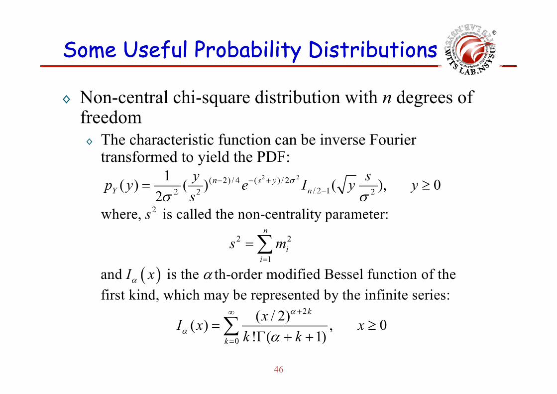
◊ Non-central chi-square distribution with n degrees of freedom◊ The characteristic function can be inverse Fourier
f d i ld h PDFtransformed to yield the PDF:2 2( 2) / 4 ( ) / 2
/ 2 12 2 2
1( ) ( ) ( ), 02
n s yY n
y sp y e I y ys
2
2 2
2where, is called the non-centrality parameter:
n
ss
s m
1
and is the th-order modified Bessel function
ii
s m
I x
of the
2
first kind, which may be represented by the infinite series:( / 2) ( ) , 0
( )
kxI x xk k
46
0
( ) ,! ( 1)k k k

Some Useful Probability DistributionsSome Useful Probability Distributions
◊ Non-central chi-square distribution with n degrees of freedom◊ The CDF is:
y
nus
n
Y dusuIesuyF
0 212/2/)(
4/2
22 )(2
1)(22
◊ The first two moments of a non-central chi-square-distributed random variable are:
s2
distributed random variable are:
22)( snYE
2242
2222242
42)(42)(
)(
snsnsnYE
47
42 sny
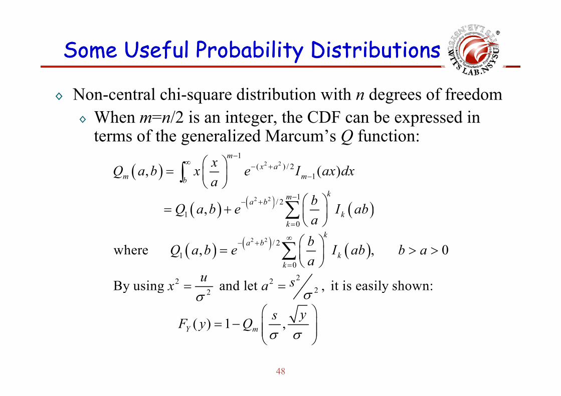
Some Useful Probability DistributionsSome Useful Probability Distributions
◊ Non-central chi-square distribution with n degrees of freedom◊ When m=n/2 is an integer, the CDF can be expressed in
terms of the generalized Marcum’s Q function:1
2 2
2 2
1( ) / 2
1
1
, ( )m
x am mb
km
xQ a b x e I ax dxa
b
2 2
2 2
1/ 21
0
/ 2
,ma b
kk
ka b
bQ a b e I aba
b
/ 21
022 2
2
where , , 0
By using and let it is easily shown:
a bk
k
bQ a b e I ab b aa
u sx a
22By using and let , it is easily shown:
x a
( ) 1 ,Y mysF y Q
48

Some Useful Probability DistributionsSome Useful Probability Distributions
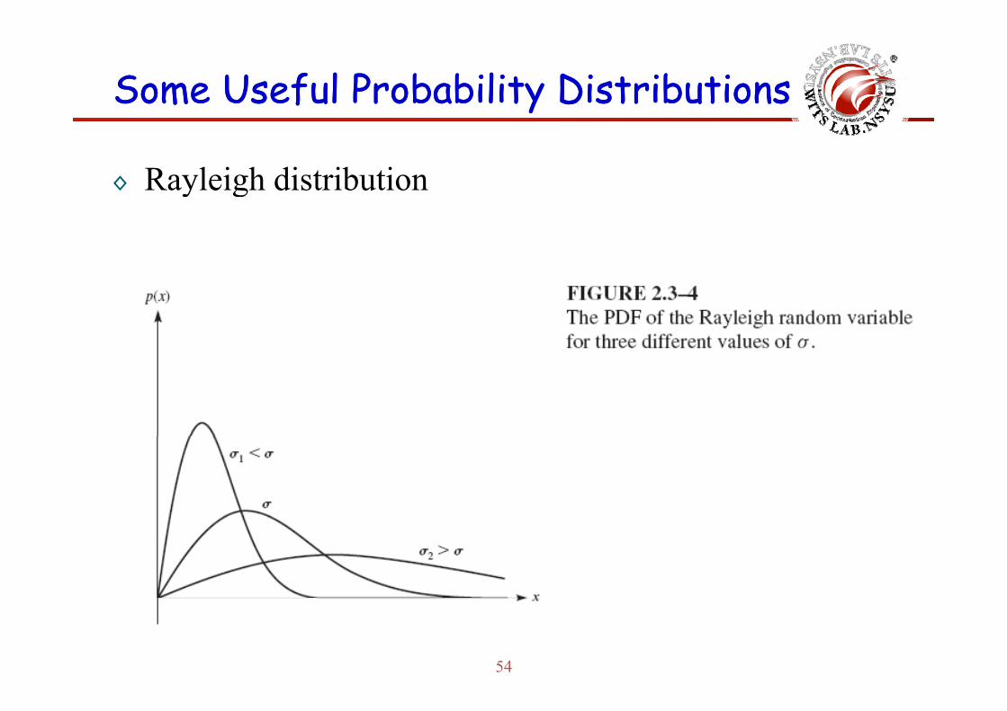
◊ Rayleigh distributiony g◊ Rayleigh distribution is frequently used to model the statistics
of signals transmitted through radio channels such as cellular radio.
◊ Consider a carrier signal s at a frequency ω0 and with an amplitude a:
)exp( 0tjas
◊ The received signal sr is the sum of n waves:
n
ii tjrtjas 00 )(exp)(exp
n
ii
iiir
jajr
tjrtjas 01
0
)exp()exp(where
)(exp)(exp
49
i
ii jajr1
)exp()exp( where
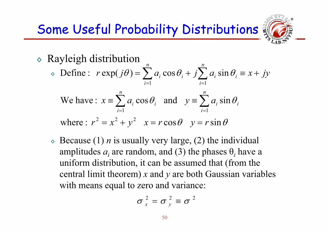
Some Useful Probability DistributionsSome Useful Probability Distributions
◊ Rayleigh distributiony g◊ sincos)exp( :Define
11
jyxajajrn
iii
n
iii
sin and cos :have We11
ayaxn
iii
n
iii
◊ Because (1) n is usually very large, (2) the individual
sin cos :where 222 ryrxyxr
◊ Because (1) n is usually very large, (2) the individual amplitudes ai are random, and (3) the phases θi have a uniform distribution, it can be assumed that (from the central limit theorem) x and y are both Gaussian variables with means equal to zero and variance:
50
222 yx
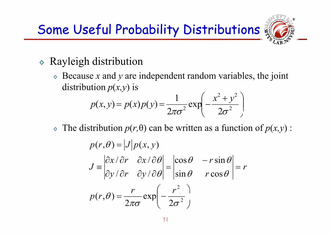
Some Useful Probability DistributionsSome Useful Probability Distributions
◊ Rayleigh distribution◊ Rayleigh distribution◊ Because x and y are independent random variables, the joint
distribution p(x,y) isp( ,y)
2
22
2 2exp
21)()(),(
yxypxpyxp
◊ The distribution p(r,θ) can be written as a function of p(x,y) :
)()( yxpJrp
sincos//
),(),(
rrxrx
J
yxpJrp
2
exp)(
cossin//
rrrp
ryry
51
22exp
2),(
rp

Some Useful Probability DistributionsSome Useful Probability Distributions
◊ Rayleigh distribution◊ Rayleigh distribution◊ Thus, the Rayleigh distribution has a PDF given by:
22 2/2 r
otherwise 0
0 ),()(22 2/
22
0
rerdrprp
r
R
◊ The probability that the envelope of the received signal does not exceed a specified value R is given by the corresponding
not exceed a specified value R is given by the corresponding cumulative distribution function (CDF):
r
0 ,exp1)(2222 2/
0
2/2 rdueurF r
ru
R
52

Some Useful Probability DistributionsSome Useful Probability Distributions
◊ Rayleigh distribution
◊ Mean: 2533.12
)(][0
drrrpRErmean
2
◊ Variance:2
0
2222
2)(][][
drrprREREr
22 4292.02
2
medianr1
◊ Median value of r is found by solving: median drrp
021
177.1medianr 2/ kk
◊ Monents of R are:
lik l l
212][ 2/2 kRE kk
53
◊ Most likely value:= max { pR(r) } = σ.
Some Useful Probability DistributionsSome Useful Probability Distributions
◊ Rayleigh distributiony g
54

Some Useful Probability DistributionsSome Useful Probability Distributions
◊ Rayleigh distributiony g◊ Probability That Received Signal Doesn’t Exceed A Certain
Level (R) )()( dFr
2
0
)()(
uu
duuprF
r
R
2
022 2
exp
duuu
r
02
2
2exp
u
2
2
2exp1
r
55

Some Useful Probability DistributionsSome Useful Probability Distributions
◊ Rayleigh distributiony g◊ Mean value:
[ ] ( )meanr E R rp r dr
0
2 2 2
2 2 2exp exp2 2
r r rdr rd
0 0
2 2
2 2
2 2
exp exp2 2r rr dr
0-0=0
2 200
2
p p2 212 exp r dr
20
2 exp22
12 1 2533
dr
56
2 1.25332 2

Some Useful Probability DistributionsSome Useful Probability Distributions
◊ Rayleigh distribution:y g◊ Mean square value:
22
223
0
22 )(][
rrr
drrprRE
20
2
022 2
exp 2
exp
rdrdrrr
0-0=0
2
2
002
22
2exp2
2exp
drrrrr0-0=0
22
22 2
2exp2
r
57
02

Some Useful Probability DistributionsSome Useful Probability Distributions
◊ Rayleigh distributiony g◊ Variance:
222 ][][
REREr
22 )2
()2(
22 4292.02
2
58

Some Useful Probability DistributionsSome Useful Probability Distributions
◊ Rayleigh distributiony g◊ Most likely value
◊ Most Likely Value happens when: dp(r) / dr = 0
021)( 222
rrrrdp
02
exp22
exp)(2422
rdrp
6065021exp
2
rr
r
6065.022
exp)( 22
rr
rrrp
59
Some Useful Probability DistributionsSome Useful Probability Distributions
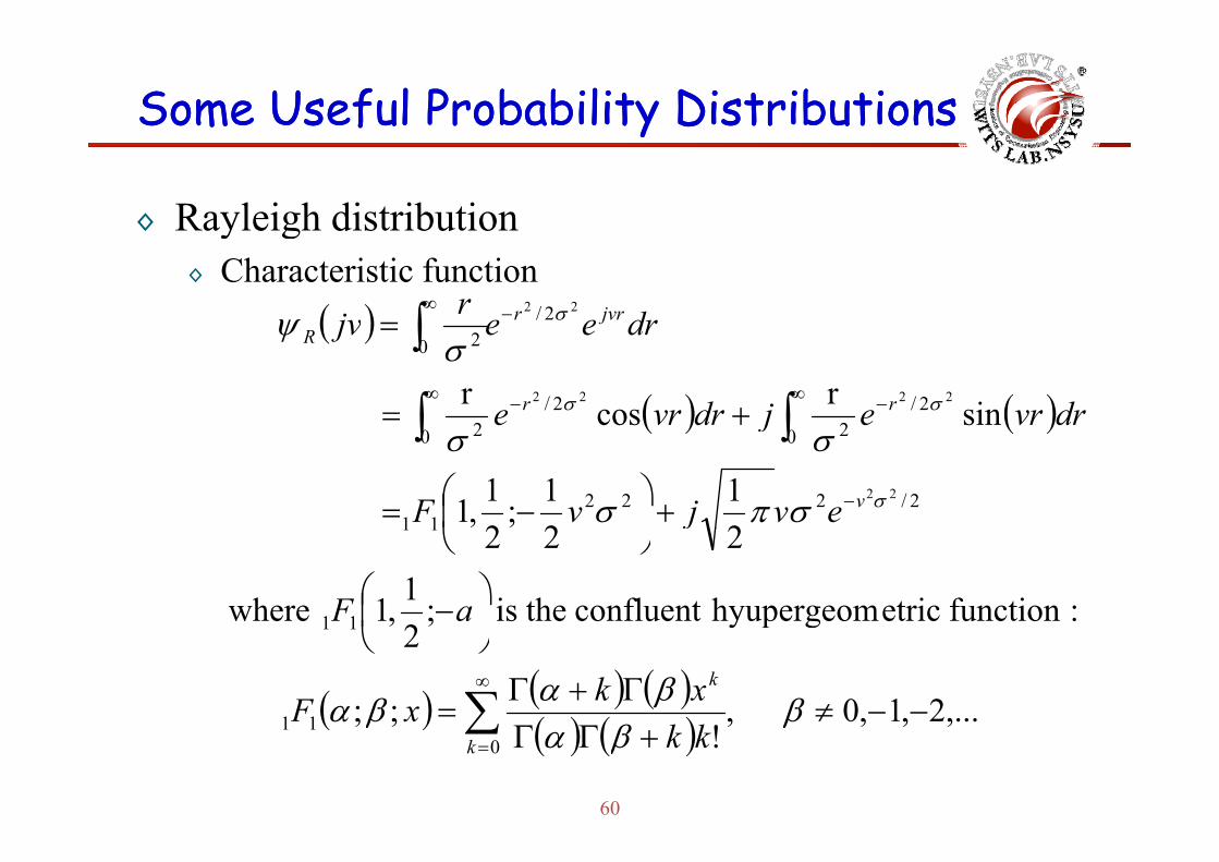
◊ Rayleigh distributiony g◊ Characteristic function
2/2
22
jvrr
R dreerjv
sinrcosr
0
2/20
2/2
0 2
2222
rr
R
drvrejdrvre
dreejv
21
21;
21,1 2/222
11
0 20 2
22
vevjvF
j
:functionetrichyupergeomconfluent theis;21,1where
222
11
11
aF
j
,...2,1,0 ,;;
y p g2
11
11
k
kkxkxF
60
,,,,!
;;0
11
k kk
Some Useful Probability DistributionsSome Useful Probability Distributions
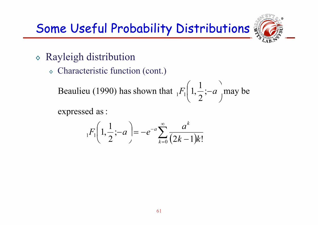
◊ Rayleigh distributiony g◊ Characteristic function (cont.)
1
11
:asexpressed
bemay ;21,1shown thathas(1990)Beaulieu aF
11 !12
;21,1
:asexpressedk
a
kkaeaF
0 !122 k kk
61
Some Useful Probability DistributionsSome Useful Probability Distributions
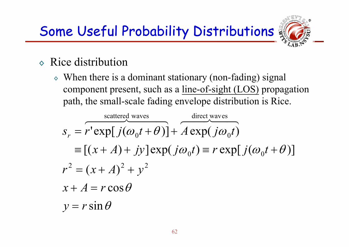
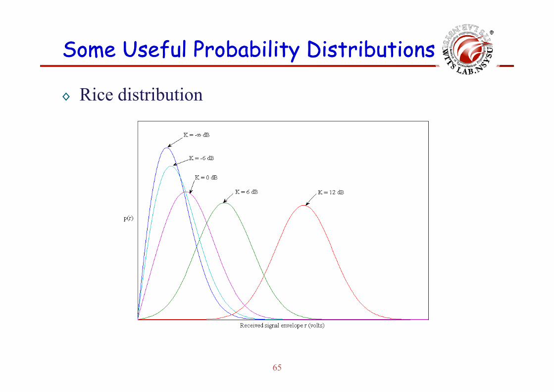
◊ Rice distribution◊ When there is a dominant stationary (non-fading) signal
component present, such as a line-of-sight (LOS) propagation path, the small-scale fading envelope distribution is Rice.
esdirect wav wavesscattered
)](exp[)exp(])[()exp()](exp['
00
00
tjrtjjyAxtjAtjrsr
)(
)](exp[)exp(])[( 222
00
yAxr
tjrtjjyAx
sincos
ryrAx
62
sinry

Some Useful Probability DistributionsSome Useful Probability Distributions
◊ Rice distribution◊ By following similar steps described in Rayleigh distribution,
we obtain:
2 2
02 2 2exp for A 0,r 0 ( ) 2r r r
r r A ArIp r
0 for 0where
(r )
2
0 2 20
1 cos exp2r r
Ar ArI d
is the modified zeroth-order Bessel function.
ixI (x)
63
00
! 2i
iI (x)
i

Some Useful Probability DistributionsSome Useful Probability Distributions
◊ Rice distribution◊ The Rice distribution is often described in terms of a
parameter K which is defined as the ratio between the d i i i i l d h i f h l i hdeterministic signal power and the variance of the multi-path. It is given by K=A2/(2σ2) or in terms of dB:
2
Th t K i k th Ri f t d l t l
2
2(dB) 10 log [dB]2AK
◊ The parameter K is known as the Rice factor and completely specifies the Rice distribution.
◊ As A0 K ∞ dB and as the dominant path decreases in◊ As A0, K-∞ dB, and as the dominant path decreases in amplitude, the Rice distribution degenerates to a Rayleigh distribution.
64
Some Useful Probability DistributionsSome Useful Probability Distributions
◊ Rice distribution
65

Some Useful Probability DistributionsSome Useful Probability Distributions
◊ Rice distribution
n
iiir tjAtjas 0
10 )exp()(exp
n
ii
i
tjAtjja 00
1
)exp()()exp(
i
tjAtjjr 00
1
)exp()exp()exp('
tjrtjjyAxtjAtjr
00
00
)(exp)exp()( )exp()(exp'
n
ii jajr
jjjy 00
)exp()exp(' where
)(e p)e p()(
66
i 1

Some Useful Probability DistributionsSome Useful Probability Distributions
◊ Rice distribution◊ sincos)exp(' :Define
11
jyxajajrn
iii
n
iii
sin and cos :have We11
ayaxn
iii
n
iii
◊ Because (1) n is usually very large, (2) the individual
sin cos )( and 222 ryrAxyAxr
◊ Because (1) n is usually very large, (2) the individual amplitudes ai are random, and (3) the phases θi have a uniform distribution, it can be assumed that (from the central limit theorem) x and y are both Gaussian variables with means equal to zero and variance:
67
222 yx

Some Useful Probability DistributionsSome Useful Probability Distributions
◊ Rice distribution◊ Because x and y are independent random variables, the joint
distribution p(x,y) is
2
22
2 2exp
21)()(),(
yxypxpyxp
◊ The distribution p(r,θ) can be written as a function of p(x,y) :
yxpJrp ),(),(
rrr
yryxrx
J
cossinsincos
////
68
ryry cossin//

Some Useful Probability DistributionsSome Useful Probability Distributions
◊ Rice distribution
2
22
2exp
2),(
yxrrp
2
22
2)sin()cos(exp
2
22
rArr
2
22 cos2exp
22
ArArr
22
2
cose p1e p
2exp
2
ArArr
22 exp
22exp
69

Some Useful Probability DistributionsSome Useful Probability Distributions
◊ Rice distribution
(pdf)function density y probabilitahason distributi RiceThe
)()(
:bygiven 2
drprp
cos1
),()(
222
0
dArArr
drprp
otherwise 0
0 cosexp21
2exp
0222 rdArArr
70

Some Useful Probability DistributionsSome Useful Probability Distributions
◊ Nakagami m-distributiong◊ Frequently used to characterize the statistics of signals
transmitted through multi-path fading channels.◊ PDF is given by Nakagami (1960) as:
2 /12 2
m mrm
m
2
/12
RE
erm
rp mrmR
21 ,
][
22
2
mRE
m
RE
figurefadingthecalled moments, of ratio theas defined is mparameter The
2][ RE
71
figure.fading the
Some Useful Probability DistributionsSome Useful Probability Distributions
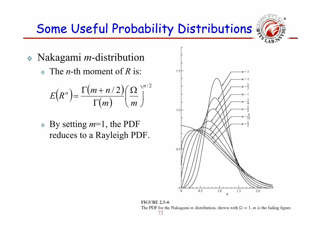
◊ Nakagami m-distributiong◊ The n-th moment of R is:
2/2/ n
2/n
mmnmRE
◊ By setting m=1, the PDF reduces to a Rayleigh PDF.y g
72

Some Useful Probability DistributionsSome Useful Probability Distributions
◊ Lognormal distribution:◊
.varianceandmean with ddistributenormally is where,lnLet
2
mXRX
◊ The PDF of R is given by:
. varianceand
2 2ln / 21 02
r me rp r r
◊ The lognormal distribution is suitable for modeling the effect
0 0r
g gof shadowing of the signal due to large obstructions, such as tall buildings, in mobile radio communications.
73

Some Useful Probability DistributionsSome Useful Probability Distributions
◊ Multivariate Gaussian distribution◊ Assume that Xi, i=1,2,…,n, are Gaussian random variables
with means mi, i=1,2,…,n; variances σi2, i=1,2,…,n; and
covariances μij, i,j=1,2,…,n. The joint PDF of the Gaussian random variables Xi, i=1,2,…,n, is defined as
xxnnxxxp mxMmxM
1
21exp
det21,...,, 2/12/21
◊ M denotes the n × n covariance matrix with elements {μij};◊ x denotes the n × 1 column vector of the random variables;◊ m denote the n × 1 column vector of mean values m i=1 2 n◊ mx denote the n × 1 column vector of mean values mi, i=1,2,…,n.◊ M-1 denotes the inverse of M.◊ x’ denotes the transpose of x.
74

Some Useful Probability DistributionsSome Useful Probability Distributions
◊ Multivariate Gaussian distribution (cont.)( )◊ Given v the n-dimensional vector with elements υi,
i=1,2,…,n, the characteristic function corresponding to the n-dimentional joint PDF is:
1j
Mvvvmv xv
21exp X
j jeEj
75

Some Useful Probability DistributionsSome Useful Probability Distributions
◊ Bi-variate or two-dimensional Gaussian◊ The bivariate Gaussian PDF is given by:
1 21,p x x
1 2 21 2
2 22 22 1 1 1 2 1 1 2 2 1 2 2
,2 1
2exp
p
x m x m x m x m
2 2 21 2
21 1 12
exp2 1
mE x m x m
m M 12 1 1 2 22
2 12 2
, ,
, , 0 1
X
ijij ij
E x m x mm
i j
m M
21 1 2
2
, ,
ij iji j
j
M
21 2 1 2
22 2 2
1, 1
M
76
21 2 2 22 2 2
1 2 11 2 1

Some Useful Probability DistributionsSome Useful Probability Distributions
◊ Bi-variate or two-dimensional Gaussian◊ ρ is a measure of the correlation between X1 and X2.◊ When ρ=0, the joint PDF p(x1,x2) factors into the product ρ , j p( 1, 2) p
p(x1)p(x2), where p(xi), i=1,2, are the marginal PDFs.◊ When the Gaussian random variables X1 and X2 are 1 2
uncorrelated, they are also statistically independent. This property does not hold in general for other distributions.
◊ This property can be extended to n-dimensional Gaussian random variables: if ρij=0 for i≠j, then the random variables Xi, i=1 2 n are uncorrelated and hence statisticallyi=1,2,…,n, are uncorrelated and, hence, statistically independent.
77

Upper Bounds on the Tail ProbabilityUpper Bounds on the Tail Probability
◊ Chebyshev inequalityy q y◊ Suppose X is an arbitrary random variable with finite mean mx
and finite variance σx2. For any positive number δ:
2
2
x
xmXP
◊ Proof:
2 2 2( ) ( ) ( ) ( )d d
2 2 2
| |
2 2
( ) ( ) ( ) ( )
( ) (| | ) x
x x xx m
x
x m p x dx x m p x dx
p x dx P X m
| |
( ) (| | )x
xx mp
78

Upper Bounds on the Tail ProbabilityUpper Bounds on the Tail Probability
◊ Chebyshev inequalityy q y◊ Another way to view the Chebyshev bound is working with
the zero mean random variable Y=X-mx.◊ Define a function g(Y) as:
E g Y g y p y dy 1 Y
g g y p y dy
p y dy p y dy P Y
2Y
1 Y
0 Yg Y
◊ Upper-bound g(Y) by the quadratic (Y/δ)2, i.e.
YYg
◊ The tail probability 2
2
2
2
2
2
2
2
xyYEYEYgE
79

Upper Bounds on the Tail ProbabilityUpper Bounds on the Tail Probability
◊ Chebychev inequalityy q y◊ A quadratic upper bound on g(Y) used in obtaining the tail
probability (Chebyshev bound)
◊ For many practical applications, the Chebyshev bound is
80
y p pp , yextremely loose.

Upper Bounds on the Tail ProbabilityUpper Bounds on the Tail Probability
◊ Chernoff bound◊ The Chebyshev bound given above involves the area under
the two tails of the PDF. In some applications we are interested only in the area under one tail, either in the interval (δ, ∞) or in the interval (-∞, δ).
◊ In such a case, we can obtain an extremely tight upper boundby over-bounding the function g(Y) by an exponential having a parameter that can be optimized to yield as tight an uppera parameter that can be optimized to yield as tight an upper bound as possible.
◊ Consider the tail probability in the interval (δ ∞)◊ Consider the tail probability in the interval (δ, ∞).
1 and is defined as
0 v Y Y δ
g Y e g Y g YY δ
81
where 0 is the parameter to be optimized.v

Upper Bounds on the Tail ProbabilityUpper Bounds on the Tail Probability◊ Chernoff bound
◊
◊ The expected value of g(Y) is
YveEYPygE
82
◊ This bound is valid for any υ 0.

Upper Bounds on the Tail ProbabilityUpper Bounds on the Tail Probability
◊ Chernoff bound◊ The tightest upper bound is obtained by selecting the value
that minimizes E(eυ(Y-δ)).◊ A necessary condition for a minimum is:
0YveEd 0eEdv
( ) ( )( ) ( )v Y v Yd dE E ( ) ( )
( )
( ) ( )
[( ) ]
v Y v Y
v Y
E e E edv dv
E Y e
[ ( ) ( )] 0v vY vYe E Ye E e
0 vYvY eEYeE Find
83
0 eEYeE Find

Upper Bounds on the Tail ProbabilityUpper Bounds on the Tail Probability
◊ Chernoff bound◊ v
:isyprobabilit tailsided-one on the boundupper thesolution, thebe ˆLet
Yvv eEeYP ˆˆ :isy probabilit
◊ An upper bound on the lower tail probability can be obtained in a similar manner, with the result that,
0 ˆˆ Yvv eEeYP
84
Upper Bounds on the Tail ProbabilityUpper Bounds on the Tail Probability
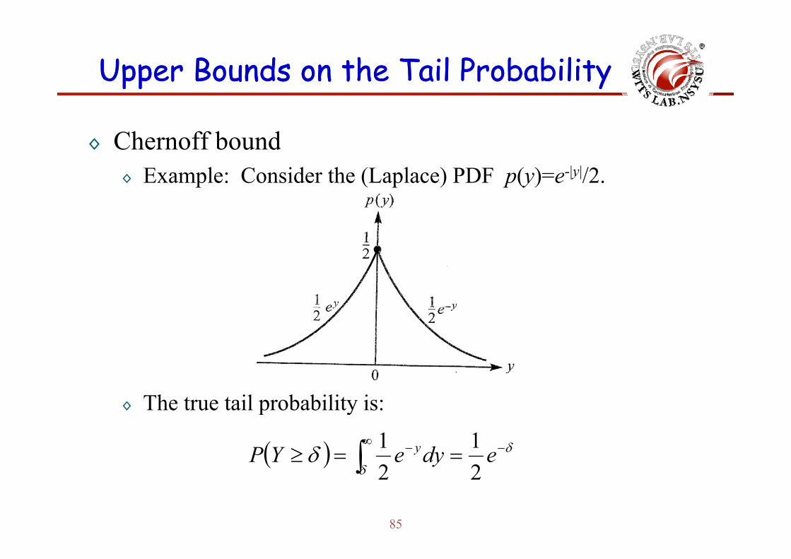
◊ Chernoff bound◊ Example: Consider the (Laplace) PDF p(y)=e-|y|/2.
◊ The true tail probability is:◊ The true tail probability is:
edyeYP y
21
21
85
22

Upper Bounds on the Tail ProbabilityUpper Bounds on the Tail Probability
◊ Chernoff bound◊ Example (cont.)
12 eEvYeE vYvY
02obtain we,0 Since
11
112
22
vveEYeE
vveE
vvYeE
vYvY
positive) bemust ˆ( 11ˆ
,2
vv
112 11
2
22
eYP
boundChebyshevfor 1 :1for
112
2
2
eYP
86
y2 2

Sums of Random Variables and the Central Limit Sums of Random Variables and the Central Limit TheoremTheorem
◊ Sum of random variables◊ Suppose that Xi, i=1,2,…,n, are statistically independent and
identically distributed (iid) random variables, each having a finite mean mx and a finite variance σx
2. Let Y be defined as the normalized sum, called the sample mean:
n
iiX
nY
1
1
◊ The mean of Y is
n
iXEmYE 1
x
iiy
m
XEn
mYE
1
87

Sums of Random Variables and the Central Limit Sums of Random Variables and the Central Limit TheoremTheorem
◊ Sum of random variables◊ The variance of Y is:◊ The variance of Y is:
mXXEmYEmYEσn n
ji222222 1
mXEXEXE
mXXEn
mYEmYEσ
n nn
i jxjixyy
22
1 12
11
mXEXEn
XEn
xi
jij
jii
i
2
1 12
12
11
nσmmnn
nmσn
n x
xxxx
222
222
2 111
◊ An estimate of a parameter (in this case the mean mx) that satisfies the conditions that its expected value converges to the true value of the parameter and the variance converges to
88
the true value of the parameter and the variance converges to zero as n→∞ is said to be a consistent estimate.

Stochastic ProcessesStochastic Processes
◊ Many of random phenomena that occur in nature are◊ Many of random phenomena that occur in nature are functions of time.
◊ In digital communications we encounter stochastic◊ In digital communications, we encounter stochastic processes in:
The characterization and modeling of signals generated by◊ The characterization and modeling of signals generated by information sources;
◊ The characterization of communication channels used to◊ The characterization of communication channels used to transmit the information;
◊ The characterization of noise generated in a receiver;◊ The characterization of noise generated in a receiver;◊ The design of the optimum receiver for processing the
received random signal.
89
g

Stochastic ProcessesStochastic Processes
◊ Introduction◊ Introduction◊ At any given time instant, the value of a stochastic process is
a random variable indexed by the parameter t. We denote y psuch a process by X(t).
◊ In general, the parameter t is continuous, whereas X may be either continuous or discrete, depending on the characteristics of the source that generates the stochastic process.
◊ The noise voltage generated by a single resistor or a single information source represents a single realization of theinformation source represents a single realization of the stochastic process. It is called a sample function.
90

Stochastic ProcessesStochastic Processes
◊ Introduction (cont.)( )◊ The set of all possible sample functions constitutes an
ensemble of sample functions or, equivalently, the stochastic process X(t).
◊ In general, the number of sample functions in the ensemble is assumed to be extremely large; often it is infinite.
◊ Having defined a stochastic process X(t) as an ensemble of l f ti id th l f thsample functions, we may consider the values of the process
at any set of time instants t1>t2>t3>…>tn, where n is any positive integerpositive integer.
◊ j ib h illi idh i
are ,,...,2,1, variablesrandom thegeneral,In i it nitXX
91
.,...,,PDFjoint by their lly statisticazedcharacteri21 nttt xxxp
Stochastic ProcessesStochastic Processes
◊ Stationary stochastic processes◊ Consider another set of random variables ,
1 2 where is an arbitrary time shift These randomit t in X X t t
i n t
1 2
1, 2,..., , where is an arbitrary time shift. These random
variables are characterized by the joint PDF , ,..., .nt t t t t t
i n t
p x x x
◊The jont PDFs of the random variables and 1 2 ,
may or may not be identical. When they are identical, i.e., wheni it t tX X ,i , ,...,n
1 2 1 2 , ,..., , ,...,
for all andn nt t t t t t t t tp x x x p x x x
t
all it is said to be stationary in the strict sensen◊ When the joint PDFs are different, the stochastic process is
non-stationary.
for all and t all , it is said to be stationary in the strict sense.n
92
y

Stochastic ProcessesStochastic Processes
◊ Averages for a stochastic process are called ensemble averages.◊
i
nn
t
dxxpxXE
Xn :as defined is variablerandom theof momentth The
◊
iiii tttt dxxpxXE
on thedependwillmomentth theofvalue thegeneral,In n
◊
.on depends of PDF theif instant timepg ,
iti tXti
allforstationaryisprocessWhen the txpxp
timeoftindependenismomentththeeconseq enca as and, time,oft independen is PDF theTherefore,
.allfor ,stationaryisprocess When the txpxpii ttt
time.oft independenismomentth thee,consequenc n
93

Stochastic ProcessesStochastic Processes
◊ Two random variables: , 1, 2.it iX X t i
◊ The correlation is measured by the joint moment:i
,t t t t t t t tE X X x x p x x dx dx
◊ Since this joint moment depends on the time instants t1 and
t2, it is denoted by φ(t1 ,t2).
1 2 1 2 1 2 1 2,t t t t t t t tp
,
◊ φ(t1 ,t2) is called the autocorrelation function of the stochastic process.
◊ For a stationary stochastic process, the joint moment is:
1 2 1 2 1 2( ) ( , ) ( ) ( )t tE X X t t t t
◊
2
' '1 1 1 1 1 1
( ) ( ) ( ) ( ) ( )t t t t t tE X X E X X E X X
(Even Function)
94
◊ Average power in the process X(t): φ(0)=E(Xt2).

Stochastic ProcessesStochastic Processes
◊ Wide-sense stationary (WSS)◊ Wide sense stationary (WSS)◊ A wide-sense stationary process has the property that the
mean value of the process is independent of time (a p p (constant) and where the autocorrelation function satisfies the condition that φ(t1,t2)=φ(t1-t2).
◊ Wide-sense stationarity is a less stringent condition than strict-sense stationarity.
◊ If not otherwise specified, any subsequent discussion in which correlation functions are involved, the less stringent condition (wide sense stationarity) is impliedcondition (wide-sense stationarity) is implied.
95

Stochastic ProcessesStochastic Processes
◊ Auto-covariance function◊ Auto covariance function◊ The auto-covariance function of a stochastic process is
defined as:
1 21 2 1 2
1 2 1 2
,
,
t tt t E X m t X m t
t t m t m t
◊ When the process is stationary, the auto-covariance function simplifies to:
1 2 1 2,t t m t m t
p
◊ For a Gaussian random process, higher-order moments can 2
1 2 1 2,t t t t m (function of time difference)
p , gbe expressed in terms of first and second moments. Consequently, a Gaussian random process is completely h i d b i fi
96
characterized by its first two moments.

Stochastic ProcessesStochastic Processes
◊ Averages for a Gaussian process◊ Suppose that X(t) is a Gaussian random process. At time
instants t=ti, i=1,2,…,n, the random variables Xti, i=1,2,…,n, are jointly Gaussian with mean values m(t ) i=1 2 n andare jointly Gaussian with mean values m(ti), i=1,2,…,n, and auto-covariances:
, , , 1, 2,..., .i j i jt t E X m t X m t i j n ◊ If we denote the n × n covariance matrix with elements μ(ti,tj)
by M and the vector of mean values by mx, the joint PDF of
, , , 1, 2,..., .i ji j t i t jt t E X m t X m t i j n
y y x, jthe random variables Xti, i=1,2,…,n, is given by:
xxxp mxMmx 11exp1
◊ If the Gaussian process is wide-sense stationary, it is also
xxnnxxxp mxMmx
M 2exp
det2,...,, 2/12/21
97
strict-sense stationary.

Stochastic ProcessesStochastic Processes
◊ Averages for joint stochastic processesg j p◊ Let X(t) and Y(t) denote two stochastic processes and let
Xti≡X(ti), i=1,2,…,n, Yt’j≡Y(t’j), j=1,2,…,m, represent the
i j jrandom variables at times t1>t2>t3>…>tn, and t’1>t’2>t’3>…>t’m , respectively. The two processes are h t i d t ti ti ll b th i j i t PDFcharacterized statistically by their joint PDF:
Th l i f i f X( ) d Y( ) d t d b ' ' '1 2 1 2
, ,..., , , ,...,n m
t t t t t tp x x x y y y
◊ The cross-correlation function of X(t) and Y(t), denoted by φxy(t1,t2), is defined as the joint moment:
)()()( ddYXEtt◊ The cross-covariance is:
21212121),()(),( 21 ttttttttxy dydxyxpyxYXEtt
)()()()( tmtmtttt
98
)()(),(),( 212121 tmtmtttt yxxyxy
Stochastic ProcessesStochastic Processes
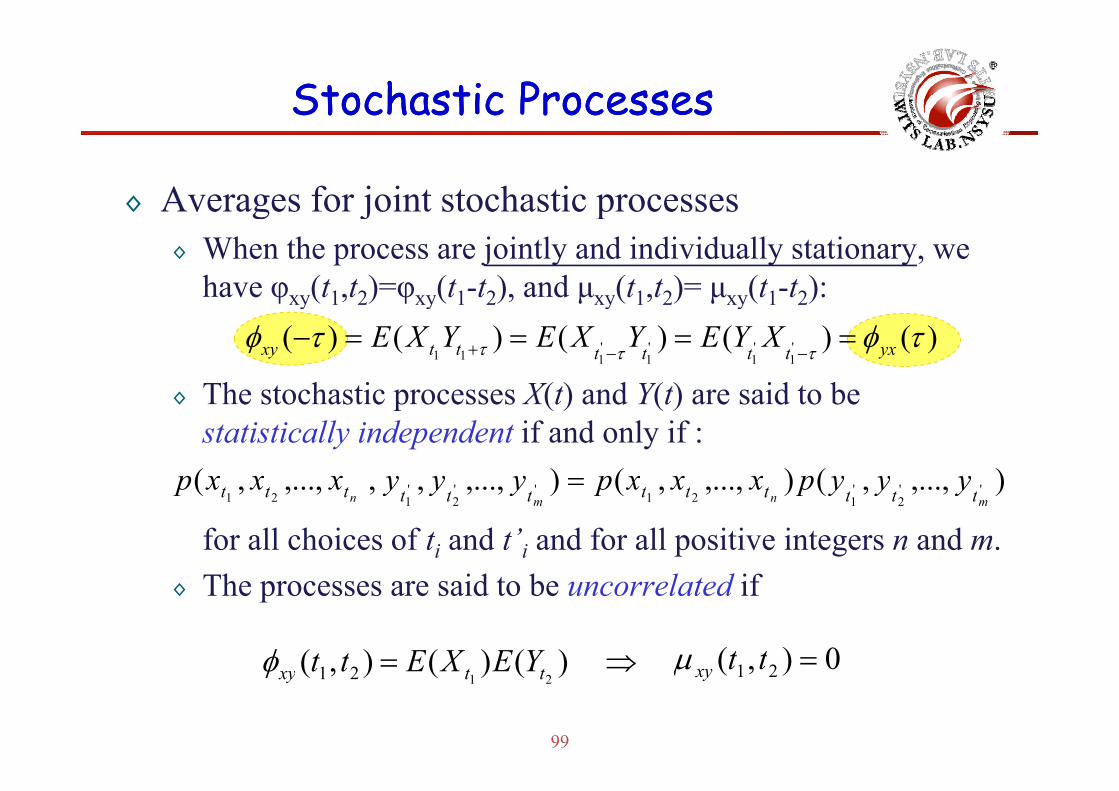
◊ Averages for joint stochastic processesg j p◊ When the process are jointly and individually stationary, we
have φxy(t1,t2)=φxy(t1-t2), and μxy(t1,t2)= μxy(t1-t2):y y y y
◊ The stochastic processes X(t) and Y(t) are said to be
' ' ' '1 1 1 1 1 1( ) ( ) ( ) ( ) ( )xy t t yxt t t t
E X Y E X Y E Y X
◊ The stochastic processes X(t) and Y(t) are said to be statistically independent if and only if :
)()()( '''''' yyypxxxpyyyxxxp
for all choices of ti and t’i and for all positive integers n and m.Th id b l d if
),...,,(),...,,(),...,,,,...,,( ''2
'121''
2'121 mnmn tttttttttttt yyypxxxpyyyxxxp
◊ The processes are said to be uncorrelated if
)()()( YEXEtt 0)( 21 tt
99
)()(),(2121 ttxy YEXEtt 0),( 21 ttxy

Stochastic ProcessesStochastic Processes◊ Complex-valued stochastic process
◊ A complex valued stochastic process Z(t) is defined as:◊ A complex-valued stochastic process Z(t) is defined as:
where X(t) and Y(t) are stochastic processes)()()( tjYtXtZ
where X(t) and Y(t) are stochastic processes.◊ The joint PDF of the random variables Zti≡Z(ti), i=1,2,…,n, is
given by the joint PDF of the components (X Y ) i=1 2 ngiven by the joint PDF of the components (Xti, Yti), i=1,2,…,n. Thus, the PDF that characterizes Zti, i=1,2,…,n, is:
),...,,,,...,,( tttttt yyyxxxp◊ The autocorrelation function is defined as:
), ,,,, ,,(2121 nn tttttt yyyp
1 1
1 2 1 1 2 21 21 1( , ) ( )2 21 ( ) ( ) ( ) ( )
zz t t t t t tt t E Z Z E X jY X jY
t t t t j t t t t
(**)
100
1 2 1 2 1 2 1 2 ( , ) ( , ) ( , ) ( , ) 2 xx yy yx xyt t t t j t t t t

Stochastic ProcessesStochastic Processes
◊ Averages for joint stochastic processes:g j p◊ When the processes X(t) and Y(t) are jointly and individually
stationary, the autocorrelation function of Z(t) becomes:
)()(),( 2121 zzzzzz tttt
1◊ φZZ(τ)= φ*
ZZ(-τ) because from (**):1 21 2
1( , ) ( )2zz t tt t E Z Z
' ' ' '1 1 1 1 1 1
1 1 1( ) ( ) ( ) ( ) ( )2 2 2zz t t zzt t t t
E Z Z E Z Z E Z Z
101

Stochastic ProcessesStochastic Processes
◊ Averages for joint stochastic processes:◊ Suppose that Z(t)=X(t)+jY(t) and W(t)=U(t)+jV(t) are two
complex-valued stochastic processes. The cross-correlation functions of Z(t) and W(t) is defined as:functions of Z(t) and W(t) is defined as:
1 21 21( , ) ( )2zw t tt t E Z W
1 1 2 2
1 21
t t t tE X jY U jV
◊ When X(t), Y(t),U(t) and V(t) are pairwise-stationary, the 1 2 1 2 1 2 1 2
1 ( , ) ( , ) ( , ) ( , ) 2 xu yv yu xvt t t t j t t t t
cross-correlation function become functions of the time difference.
◊1 1 1( ) ( ) ( ) ( ) ( )E Z W E Z W E W Z
102
◊ ' ' ' '1 1 1 1( ) ( ) ( ) ( ) ( )
2 2 2i izw t t wzt t t t
E Z W E Z W E W Z

Power Density SpectrumPower Density Spectrumy py p
◊ A signal can be classified as having either a finite (nonzero) average power (infinite energy) or finite energy.
◊ The frequency content of a finite energy signal is obtained q y gy gas the Fourier transform of the corresponding time function.
◊ If the signal is periodic, its energy is infinite and, consequently its Fourier transform does not exist Theconsequently, its Fourier transform does not exist. The mechanism for dealing with periodic signals is to represent them in a Fourier seriesthem in a Fourier series.
103

Power Density SpectrumPower Density Spectrum
◊ A stationary stochastic process is an infinite energy y p gysignal, and, hence, its Fourier transform does not exist.
◊ The spectral characteristic of a stochastic signal is◊ The spectral characteristic of a stochastic signal is obtained by computing the Fourier transform of the autocorrelation function.autocorrelation function.
◊ The distribution of power with frequency is given by the function:the function:
def fj 2
◊ The inverse Fourier transform relationship is:
dff fj 2
104
dfef fj 2

Power Density SpectrumPower Density Spectrum
◊ 00 2
tXEdff◊ Since φ(0) represents the average power of the stochastic signal,
which is the area under Φ(f ), Φ(f ) is the distribution of power as
a function of frequency.◊ Φ( f ) is called the power density spectrum of the stochastic
process.◊ If the stochastic process is real, φ(τ) is real and even, and, hence Φ( f ) is real and e en
(from definition)
(P.94)( t f d fi iti )Φ( f ) is real and even.
◊ If the stochastic process is complex, φ(τ)=φ*(-τ) and Φ( f ) is real because:
( )
(P.101)
(easy to prove from definition)
real because:
* * 2 * 2 '
2
' 'j f j f
j f
f e d e d
d f
( )
105
2 j fe d f

Power Density SpectrumPower Density Spectrum
◊ Cross-power density spectrump y p◊ For two jointly stationary stochastic processes X(t) and Y(t),
which have a cross-correlation function φxy(τ), the Fourier ytransform is:
def fjxyxy
2
◊ Φxy( f ) is called the cross-power density spectrum.◊ dedef fj
xyfj
xyxy
2*2**
fde yxfj
yx
yyy
2
◊ If X(t) and Y(t) are real stochastic processes
* 2j ff e d f
f f →
106
xy xy xyf e d f
yx xyf f →

Response of a Linear TimeResponse of a Linear Time--Invariant System to a Invariant System to a Random Input SignalRandom Input Signal
◊ Consider a linear time-invariant system (filter) that is characterized by its impulse response h(t) or equivalently, by its
p gp g
frequency response H( f ), where h(t) and H( f ) are a Fourier transform pair. Let x(t) be the input signal to the system and let y(t) denote the output signaly(t) denote the output signal.
y t h x t d
◊ Suppose that x(t) is a sample function of a stationary stochastic process X(t). Since convolution is a linear operation performed on the input signal x(t) the expected value of the integral ison the input signal x(t), the expected value of the integral is equal to the integral of the expected value.
ym E Y t h E X t d
0
y
x xm h d m H
stationary
107
◊ The mean value of the output process is a constant.

Response of a Linear TimeResponse of a Linear Time--Invariant System to a Invariant System to a Random Input SignalRandom Input Signal
◊ The autocorrelation function of the output is:
p gp g
YYEtt ttyy*
21 21,
21
ddtXtXEhh 2
*1
*
21
ddtthh xx 21
*
◊ If the input process is stationary, the output is also stationary:
*yy xxh h d d
108
Response of a Linear TimeResponse of a Linear Time--Invariant System to a Invariant System to a Random Input SignalRandom Input Signal
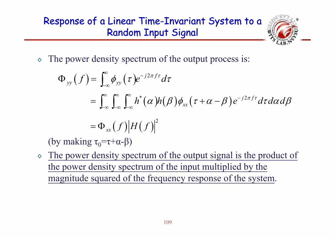
◊ The power density spectrum of the output process is:
p gp g
2j fyy yyf e d
* 2j fxxh h e d d d
(by making τ0=τ+α-β) 2
xx f H f
( y g 0 β)◊ The power density spectrum of the output signal is the product of
the power density spectrum of the input multiplied by the magnitude squared of the frequency response of the system.
109

Response of a Linear TimeResponse of a Linear Time--Invariant System to a Invariant System to a Random Input SignalRandom Input Signal
◊ When the autocorrelation function φyy(τ) is desired, it is usually
p gp g
yyeasier to determine the power density spectrum Φyy(f ) and then to compute the inverse transform.
2yy
j fyy f e df
2 2j ff H f e df
◊ The average power in the output signal is:
xxj ff H f e df
2xx0yy f H f df
◊ Since φyy(0)=E(|Yt|2) , we have:
20f H f df
valid for any H( f )
110
xx 0f H f df valid for any H( f ).
Response of a Linear TimeResponse of a Linear Time--Invariant System to a Invariant System to a Random Input SignalRandom Input Signal
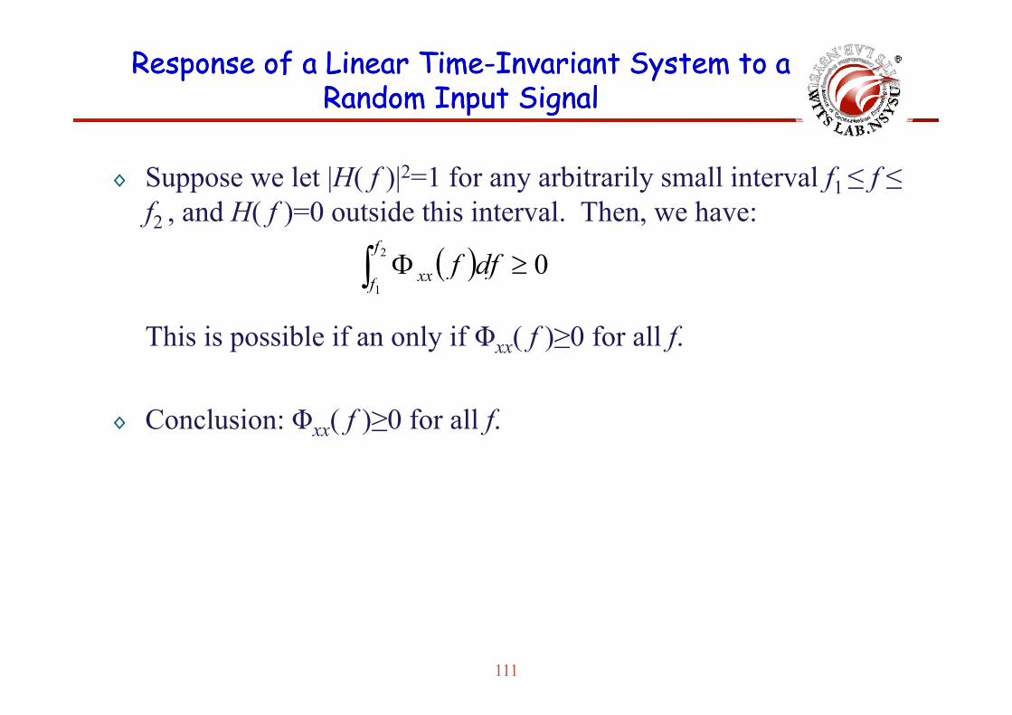
◊ Suppose we let |H( f )|2=1 for any arbitrarily small interval f1 ≤ f ≤
p gp g
f2 , and H( f )=0 outside this interval. Then, we have:
2 0f
xx dff
This is possible if an only if Φxx( f )≥0 for all f.
1f
xx ff
◊ Conclusion: Φxx( f )≥0 for all f.
111
Response of a Linear TimeResponse of a Linear Time--Invariant System to a Invariant System to a Random Input SignalRandom Input Signal
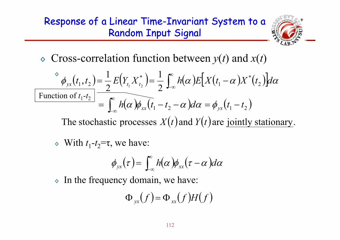
◊ Cross-correlation function between y(t) and x(t)
p gp g
◊ 21
21, 2
*1
*21 21
dtXtXEhXYEtt ttyx
i f
t tij i tldt h tiTh
2121
tYtX
ttdtth yxxx
Function of t1-t2
◊ With t1-t2=τ, we have:
.stationaryjointly are andprocessesstochastic The tYtX
1 2 ,
dh xxyx
◊ In the frequency domain, we have:
fHff xxyx
112
fff xxyx

DiscreteDiscrete--Time Stochastic Signals and SystemsTime Stochastic Signals and Systems
◊ Discrete-time stochastic process X(n) consisting of an ensemble
g yg y
of sample sequences {x(n)} are usually obtained by uniformly sampling a continuous-time stochastic process.
◊ The mth moment of X(n) is defined as:
nnmn
mn dXXpXXE
◊ The autocorrelation sequence is:
nnnn p
knknknkn dXdXXXpXXXXEkn ,
21
21, **
◊ The auto-covariance sequences is:
*1,, kn XEXEknkn
113
2
,, knknkn

DiscreteDiscrete--Time Stochastic Signals and SystemsTime Stochastic Signals and Systems
◊ For a stationary process, we have φ(n,k)≡φ(n-k), μ(n,k)≡μ(n-k), d
g yg y
and 2
21
xmknkn
where mx=E(Xn) is the mean value.◊ A discrete-time stationary process has infinite energy but a◊ A discrete time stationary process has infinite energy but a
finite average power, which is given as:
2 0E X
◊ The power density spectrum for the discrete-time process is obtained by computing the Fourier transform of φ(n)
0nE X
obtained by computing the Fourier transform of φ(n).
fnjenf 2
114
n
f
DiscreteDiscrete--Time Stochastic Signals and SystemsTime Stochastic Signals and Systems
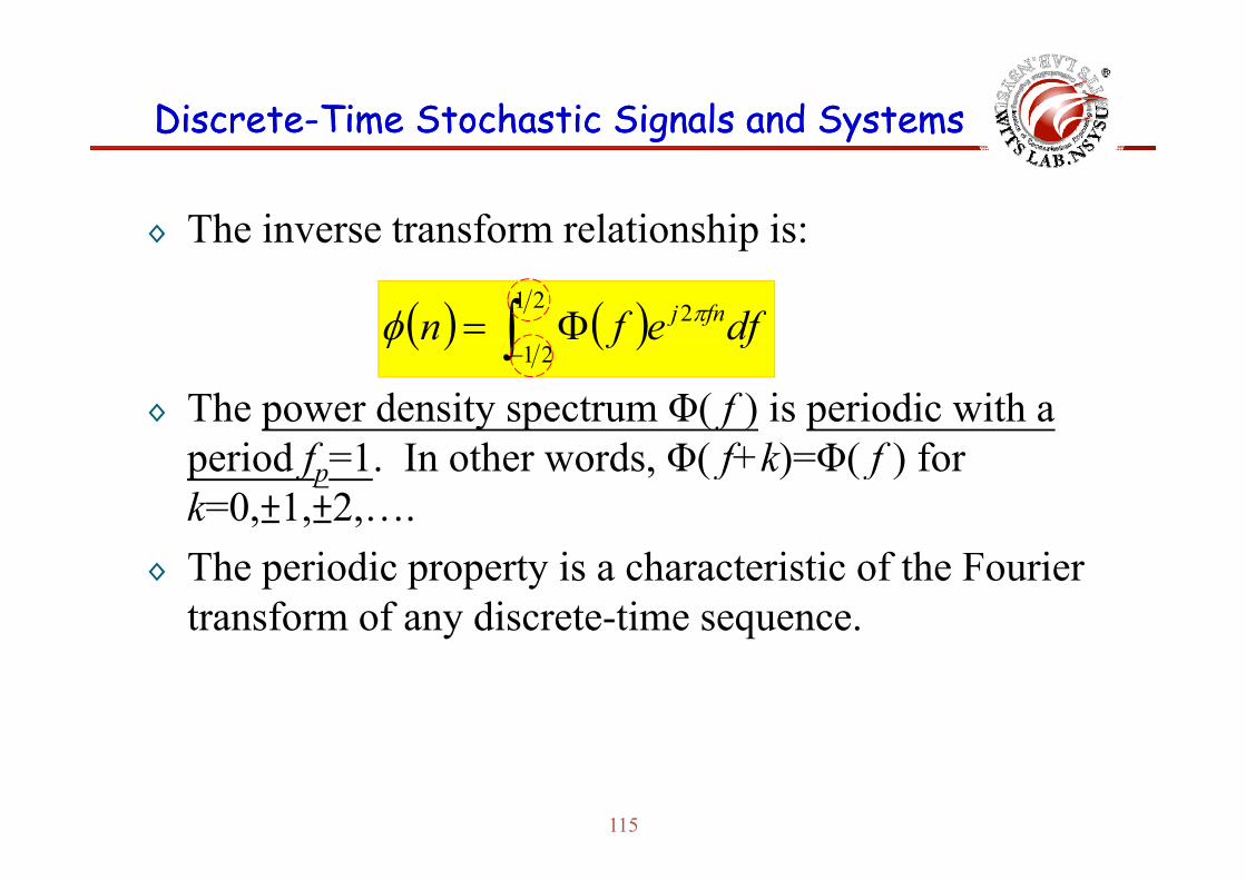
◊ The inverse transform relationship is:
g yg y
◊ The inverse transform relationship is:
21 2 dfefn fnj
◊ The power density spectrum Φ( f ) is periodic with a
21ff
period fp=1. In other words, Φ( f+k)=Φ( f ) for k=0,±1,±2,….
◊ The periodic property is a characteristic of the Fourier transform of any discrete-time sequence.
115

DiscreteDiscrete--Time Stochastic Signals and SystemsTime Stochastic Signals and Systems
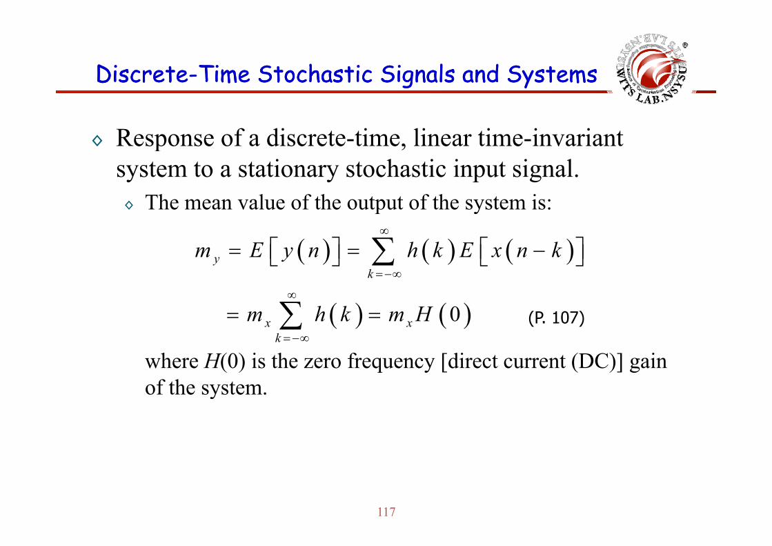
◊ Response of a discrete-time, linear time-invariant
g yg y
p ,system to a stationary stochastic input signal.◊ The system is characterized in the time domain by its unit y y
sample response h(n) and in the frequency domain by the frequency response H( f ).
n
fnjenhfH 2
◊ The response of the system to the stationary stochastic input signal X(n) is given by the convolution sum:
knxkhny
116
k
DiscreteDiscrete--Time Stochastic Signals and SystemsTime Stochastic Signals and Systems
◊ Response of a discrete-time, linear time-invariant
g yg y
p ,system to a stationary stochastic input signal.◊ The mean value of the output of the system is:p y
yk
m E y n h k E x n k
0
k
x xk
m h k m H
(P. 107)
where H(0) is the zero frequency [direct current (DC)] gain of the system.
k
y
117

DiscreteDiscrete--Time Stochastic Signals and SystemsTime Stochastic Signals and Systems◊ The autocorrelation sequence for the output process is:
1k E k
g yg y
12
1
yy k E y n y n k
h i h j E x n i x n k j
2 i j
h i h j E x n i x n k j
h i h j k j i
◊ By taking the Fourier transform of φ (k) we obtain the
xxi j
h i h j k j i
◊ By taking the Fourier transform of φyy(k), we obtain the corresponding frequency domain relationship:
2f f H f
◊ Φyy( f ), Φxx( f ), and H( f ) are periodic functions of
yy xxf f H f (P. 109)
118
◊ Φyy( f ), Φxx( f ), and H( f ) are periodic functions of frequency with period fp=1.

CCyclostationaryyclostationary ProcessesProcesses
◊ For signals that carry digital information, we encounter h i i h i i l h i distochastic processes with statistical averages that are periodic.
◊ Consider a stochastic process of the form:
nn
X t a g t nT
where {an} is a discrete-time sequence of random variables with mean ma=E(an) for all n and autocorrelation sequence φ (k)=E(a* a )/2φaa(k)=E(a*nan+k)/2.
◊ The signal g(t) is deterministic.◊ The sequence {a } represents the digital information sequence◊ The sequence {an} represents the digital information sequence
that is transmitted over the communication channel and 1/Trepresents the rate of transmission of the information symbols.
119
ep ese ts t e ate o t a s ss o o t e o at o sy bo s.

CyclostationaryCyclostationary ProcessesProcesses
◊ The mean value is:
nn
E X t E a g t nT
The mean is time varying and it is periodic with period T
an
m g t nT
The mean is time-varying and it is periodic with period T.
◊ The autocorrelation function of X(t) is:
12
1
,xx t t E X t X t
E T T
12 n m
n m
E a a g t nT g t mT
T T
120
aan m
m n g t nT g t mT

CyclostationaryCyclostationary ProcessesProcesses
◊ We observe that
for k=±1,±2,…. Hence, the autocorrelation function of X(t) is also , ,xx xxt kT t kT t t
periodic with period T.◊ Such a stochastic process is called cyclostationary or periodically
stationary.◊ Since the autocorrelation function depends on both the variables t
d i f d i i i h fand τ, its frequency domain representation requires the use of a two-dimensional Fourier transform.The ti t l ti f ti over a single period is◊ The time-average autocorrelation function over a single period is defined as:
2
2
1 ,T
xx xxTt t dt
T
121
2xx xxTT

CyclostationaryCyclostationary ProcessesProcesses
◊ Thus, we eliminate the tie dependence by dealing with the average autocorrelation function.
◊ The Fourier transform of φxx(τ) yields the average power density spectrum of the cyclostationary stochastic process.
◊ This approach allows us to simply characterize cyclostationaryi th f d i i t f th tprocess in the frequency domain in terms of the power spectrum.
◊ The power density spectrum is:
2j fxx xxf e d
122