INTRODUCTION TO PROBABILITY THEORY AND STOCHASTIC PROCESSES … · 2018-09-04 · INTRODUCTION TO...

INTRODUCTION TO PROBABILITY THEORY

AND STOCHASTIC PROCESSES

FOR UNDERGRADUATE STUDENTS

ANDREY SARANTSEV

Contents

1. Combinatorics and Binomial Coefficients 22. Basic Probability: Events and Axioms 73. Discrete Random Variables 144. Common Discrete Distributions 215. Continuous Random Variables 276. Central Limit Theorem 387. Introduction to Statistics 428. Generating and Moment Generating Functions 449. Probabilistic Inequalities and the Law of Large Numbers 4910. Conditional Expectation and Conditional Distribution 5311. Discrete-Time Markov Chains with Applications 5712. Random Walk and the Binomial Model in Finance 6713. Discrete-Time Martingales and American Derivatives 7414. Poisson Process and Compound Poisson Process 7815. Continuous-Time Markov Chains 8216. Queueing Theory 9117. Brownian Motion and the Black-Scholes Model 9318. Stochastic Calculus and Hedging Derivatives 10219. Stochastic Differential Equations 10720. Continuous-Time Martingales and American Derivatives 10921. Appendix. Simulations 113

Introduction

These are lecture notes on Probability Theory and Stochastic Processes. These include both discrete- andcontinuous-time processes, as well as elements of Statistics. These lecture notes are intended for junior- and senior-level undergraduate courses. They contain enough material for two semesters or three quarters. These lecturenotes are suitable for mathematics, applied mathematics, economics and statistics majors, but are likely too hardfor business and humanities majors. Prerequisites include matrix algebra and calculus: a standard two-semester orthree-quarter sequence, including multivariable calculus. We consider applications to insurance, finance and socialsciences, as well as some elementary statistics. We tried to keep notes as condensed and concise as possible, veryclose to the actual notes written on the board during lectures.

Acknowledgements

I am thankful to Tomoyuki Ichiba and Raya Feldman, who mentored me when I started teaching at the De-partment of Statistics and Applied Probability, University of California, Santa Barbara. I am grateful to JudithArms and Andrew Loveless, my teaching mentors at the Department of Mathematics, University of Washington.In addition, I would like to thank Janko Gravner from Department of Mathematics, University of California, Davis,who put his lecture notes on Probability and Markov Chains on his web page. These lecture notes use his materialsa lot. Last but not least, I am thankful to Soumik Pal, my Ph.D. adviser, Ioannis Karatzas, his Ph.D. adviser,Jean-Pierre Fouque, my postdoctoral mentor, and all my graduate and undergraduate probability teachers, forhelping understand and appreciate this exciting area of mathematics.

Date: August 10, 2018. Department of Statistics and Applied Probability. University of California, Santa Barbara. Email:

[email protected] .

2 ANDREY SARANTSEV

1. Combinatorics and Binomial Coefficients

1.1. Permutations. A permutation of 123 is, say, 321 or 231: numbers cannot repeat. There are 3 · 2 · 1 = 3! = 6permutations: there are 3 chioces for the first slot, 2 choices for the second slot (because one of the numbers isalready in the first slot and cannot be repeated), and only one choice for the last, third slot.

In general, for 1, 2, 3, . . . , n− 1, n there are

n! = 1 · 2 · 3 · . . . · (n− 1) · n

permutations. This number is called n factorial. Examples:

1! = 1, 2! = 2, 3! = 6, 4! = 24, 5! = 120, 6! = 720.

There is a convention that 0! = 1. Indeed, we have the property (n− 1)!n = n! for n = 2, 3, 4, . . .. It follows fromthe definition of the factorial, and this is the main property. We would like it to be true also for n = 1: 0! · 1 = 1!,so 0! = 1. Factorial grows very quickly. Indeed, 100! is extremely large; no modern computer can go throughpermutations of 1, 2, . . . , 100. When a computer programming problem encounters search among permutations ofn numbers, then this problem is deemed unsolvable. Stirling’s formula:

n! v√

2πn(ne

)nas n→∞

where f(n) v g(n) means limn→∞ f(n)/g(n) = 1.If we have three slots for numbers 1, 2, 3, 4, 5, 6, 7, and repetitions are not allowed, this is called an arrangement.

Say, 364, 137, 634. There are 7 · 6 · 5 = 210 such arrangements: 7 choices for the first slot, 6 for the second and 5for the third. We can write this as

A37 = 7 · 6 · 5 =

7 · 6 · 5 · 4 · 3 · 2 · 14 · 3 · 2 · 1 =

7!

(7− 3)!.

In general, if there are k slots for 1, 2, . . . , n, then the number of arrangements is

Akn = n · (n− 1) · (n− 2) · . . . · (n− k + 1) =n!

(n− k)!.

A permutation can be viewed as a particular case of an arrangement, when k = n: the number of slots is the sameas the total number of elements.

1.2. Subsets. How many subsets of three elements are there in the set 1, 2, . . . , 7? The difference between anarrangement and a subset is that for a subset, order does not matter. (But in both of them, there are no repetitions.)For example, 3, 4, 6 and 6, 3, 4 is the same subset, but 346 and 634 are different arrangements. From any subset,we can create 3! = 6 arrangements. So the quantity of subsets is equal to the quantity of arrangements divided by6:

A37

3!=

7!

4!3!=

210

6= 35.

In general, the quantity of subsets of k elements in 1, . . . , n is equal to(n

k

)=Aknk!

=n · (n− 1) · . . . · (n− k + 1)

k!=

n!

(n− k)!k!

It is pronounced as “n choose k”.(i)(

10

)= 1, because there is only one subset of zero elements in 1, and this is an empty set ∅.

(ii)(

11

)= 1, because there is only one subset of one element in 1: the set 1 itself.

(iii)(n0

)= 1, for the same reason as in (i);

(iv)(nn

)= 1, for the same reason as in (ii);

(v)(

21

)= 2, because there are two subsets of one element of 1, 2: these are 1 and 2;

(vi)(n1

)= n, because there are n subsets of one element of 1, 2, . . . , n: 1, 2, . . . , n;

(vii)(nn−1

)= n, because to choose a subset of n − 1 elements out of 1, 2, . . . , n, we need to throw away one

element, and it can be chosen in n ways;(viii)

(42

)= 4!/(2!2!) = 24/4 = 6, and these subsets of 1, 2, 3, 4 are

1, 2, 1, 3, 1, 4, 2, 3, 2, 4, 3, 4.

PROBABILITY THEORY AND STOCHASTIC PROCESSES 3

1.3. Symmetry. We can say without calculations that(

82

)=(

86

). Indeed, for every subset of 1, 2, . . . , 8 of two

elements there is a subset of six elements: its complement. For example, 3, 5 corresponds to 1, 2, 4, 6, 7, 8. Thisis a one-to-one correspondence. So there are equally many subsets of two elements and subsets of six elements.Similarly,

(83

)=(

85

). More generally, (

n

k

)=

(n

n− k

)1.4. Power set. How many subsets does the set 1, 2, . . . , n contain? Answer: 2n. Indeed, to construct anarbitrary subset E, you should answer n questions:

• Is 1 ∈ E? Yes/No• Is 2 ∈ E? Yes/No• . . .• Is n ∈ E? Yes/No

For each question, there are two possible answers. The total number of choices is 2 · 2 · . . . · 2︸︷︷︸n times

= 2n. The set of all

subsets of 1, . . . , n is called a power set, and it contains 2n elements. But we can also write the quantity of allsubsets as the sum of binomial coefficients:(

n

0

)+

(n

1

)+

(n

2

)+ . . .+

(n

n

).

So we get the following identity: (n

0

)+

(n

1

)+ . . .+

(n

n

)= 2n

Example 1.1. Let n = 2. Yes-Yes: E = 1, 2, Yes-No: E = 2, No-Yes: E = 1, No-No: E = ∅. Total numberof subsets: 22 = 4. Two of them have one element:

(21

)= 2, one has two elements,

(22

)= 1, and one has zero

elements,(

20

)= 1. Total: 1 + 2 + 1 = 4.

1.5. Reduction property. We can claim that(5

2

)=

(4

2

)+

(4

1

).

Indeed, the total number of subsets E ⊆ 1, 2, 3, 4, 5 which contain two elements is(

52

). But there are two

possibilities:Case 1. 5 ∈ E. Then E \ 5 is a one-element subset of 1, 2, 3, 4; there are

(41

)such subsets.

Case 2. 5 /∈ E. Then E is a two-element subset of 1, 2, 3, 4. There are(

42

)such subsets.

So(

41

)+(

42

)=(

52

). In general, (

n

k

)=

(n− 1

k

)+

(n− 1

k − 1

)1.6. Pascal’s triangle.

n = 0: 1

n = 1: 1 1

n = 2: 1 2 1

n = 3: 1 3 3 1

n = 4: 1 4 6 4 1

n = 0:(

00

)n = 1:

(10

) (11

)n = 2:

(20

) (21

) (22

)n = 3:

(30

) (31

) (32

) (33

)n = 4:

(40

) (41

) (42

) (43

) (44

)

4 ANDREY SARANTSEV

Each element is the sum of two elements immediately above it: this is the reduction formula. We start fromthe edges, fill them with ones:

(n0

)=(nn

)= 1, see the previous lecture. Then we fill the inside from top to bottom

using this rule, which is the reduction formula.

1.7. Newton’s binomial formula. We can expand (x+y)2 = x2 +2xy+y2, and (x+y)3 = x3 +3x2y+3xy2 +y3.The coefficients are taken from corresponding lines in Pascal’s triangle. Why is this? Let us show this for n = 3.

(x+ y)3 = (x+ y)(x+ y)(x+ y) = xxx+ xxy + xyx+ yxx+ xyy + yxy + yyx+ yyy.

Each term has slots occupied by y: xxy ↔ 3, yxy ↔ 1, 3. If there is one slot occupied by y, this correspondsto x2y, and there are

(31

)such combinations. So we have:

(31

)x2y. Other terms give us:(

3

0

)x3 +

(3

1

)x2y +

(3

2

)xy2 +

(3

3

)y3.

The general formula looks like this:

(x+ y)n =

(n

0

)xn +

(n

1

)xn−1y + . . .+

(n

n

)yn

Let x = y = 1. Then we get:

2n =

(n

0

)+

(n

1

)+ . . .+

(n

n

).

This formula was already proven above. Let x = 1, y = −1. Then

0 =

(n

0

)−(n

1

)+

(n

2

)−(n

3

)+ . . . ,(

n

0

)+

(n

2

)+ . . . =

(n

1

)+

(n

3

)+ . . .

The quantity of subsets with even number of elements is equal to the quantity of subsets with odd number ofelements.

1.8. Combinatorics problems. Here, we study a few combinatorics (counting) problems, which can be reducedto counting permutations and combinations.

Example 1.2. Five women and four men take an exam. We rank them from top to bottom, according to theirperformance. There are no ties.

(a) How many possible rankings?(b) What if we rank men and women separately?(c) As in (b), but Julie has the third place in women’s rankings.

(a) A ranking is just another name for permutation of nine people. The answer is 9!

(b) There are 5! permutations for women and 4! permutations for men. The total number is 5!4! We shouldmultiply them, rather than add, because men’s and women’s rankings are independent: we are interested in pairs:the first item is a ranking for women, the second item is a ranking for men. If we needed to choose: either rankwomen or rank men, then the solution would be 5! + 4!

(c) We exclude Julie from consideration, because her place is already reserved. There are four women remaining,

so the number of permutations is 4! For men, it is also 4! The answer is 4!2

Example 1.3. A licence plate consists of seven symbols: digits or letters. How many licence plates are there if thefollowing is true:

(a) there must be three letters and four digits, and symbols may repeat?(b) there must be three letters and four digits, and symbols may not repeat?(c) no restrictions on the quantity of letters and numbers, and symbols may repeat?(d) no restrictions on the quantity of letters and numbers, and symbols may not repeat?

(a) Choose three slots among seven for letters; this may be done in(

73

)ways. Fill each of these three slots with

letters; there are 263 ways to do this, since letters can repeat. Fill each of the remaining four slots with digits;

there are 104 ways to do this, since numbers can repeat. Answer:

(7

3

)· 263 · 104


(b) This case is different from (i) because there are 26 · 25 · 24 = 26!/23! ways to fill three chosen slots for letters,

and 10 · 9 · 8 · 7 = 10!/6! ways to fill four chosen slots for numbers. Answer:

(7

3

)26 · 25 · 24 · 10 · 9 · 8 · 7

(c) This case is easier than the previous ones, since there are 36 symbols, and each of the seven slots can be

filled with any of these symbols. Answer: 367

(d) Similarly to (c), 36 · 35 · 34 · 33 · 32 · 31 · 30 = 36!/29!

Example 1.4. We have five women and four men. We need to choose a committee of three women and two men.How many ways are there to do this if:

(a) there are no additional restrictions?(b) Mike and Thomas refuse to serve together?(c) Britney and Lindsey refuse to serve together?(d) Andrew and Anna refuse to serve together?

(a) There are(

42

)= 6 ways to choose two men out of four, and there are

(53

)= 10 ways to choose two women

out of five. So the answer is 60(b) How many committees are there for which this restriction is violated, so Mike and Thomas do serve together?

If they are already chosen, then we do not need to choose any other man, and there are(

53

)= 10 ways to choose

three women out of five. So the quantity of committees where Mike and Thomas do serve together is 10. The

answer is 60− 10 = 50

(c) Similarly to (b), the number of committees where Britney and Lindsay serve together is(

31

)(42

)= 18, because

you can choose one more woman out of the remaining three in(

31

)= 3 ways, and the number of choices for men is(

42

). So the answer is 60− 18 = 42

(d) Similarly to (c), the number of committees where Andrew and Anna serve together is(

31

)(42

)= 18, because

you can choose one more man out of the remaining three in(

31

)= 3 ways, and two more women out of the remaining

four in(

42

)ways. So the answer is 60− 18 = 42

Problems

Problem 1.1. There are 8 apartments for 6 people. Each person chooses one apartment, and each apartment canhost no more than one person. How many choices are there?

For the next three problems, consider the following setup. There are 10 Swedes, 7 Finns and 6 Danes; we shouldchoose a committee that consists of 9 people, three from each nation. Find the number of choices if:

Problem 1.2. There are no additional constraints.

Problem 1.3. Two of 10 Swedes refuse to serve together.

Problem 1.4. There is a Swede and a Dane who refuse to serve together?

For the next three problems, find the number of arrangements of letters in the words:

Problem 1.5. Seattle.

Problem 1.6. Alaska.

Problem 1.7. Spokane.

Problem 1.8. We need to choose a committee of six people: three French and three Germans, out of six Frenchand seven Germans. How many ways are there to do this? Your answer should be in the form of a number, say 10or 23.

Problem 1.9. Old license plates consist of six symbols: three digits and three numbers (at any place, not necessarilydigits first). Symbols cannot repeat. How many such plates are there?

For the next three problems, consider the following setup. Anna, Brendan, Christine, Daniel and Emily form aband with 5 instruments: a piano, a flute, a trombone, a violin and a guitar. Find the number of arrangements if:

Problem 1.10. Each of them can play all the instruments, and there is a rule that no two people can play thesame instrument.

Problem 1.11. Each of them can play all the instruments, and there is not a rule that no two people can playthe same instrument: for example, all of them can choose piano, so there will be five pianos in the band.

6 ANDREY SARANTSEV

Problem 1.12. Each of them can play all the instruments, and there is a rule that no two people can play thesame instrument, but they need Anna or Brendan for the trombone.

For the next three problems,consider following setup. Ten married couples (husband-wife) come to the dancinglesson. They are split into ten dancing couples, each of which contains a male and a female. Partners are assignedrandomly. Find the number of possible outcomes in the following cases:

Problem 1.13. There are no additional restrictions.

Problem 1.14. Mr Smith does not want to dance with his wife.

Problem 1.15. One of the women is tired, so now there are 9 dancing pairs (and one idle husband).

Problem 1.16. You need to select a governing committee board for an insurance company. This board shouldcontain 4 actuaries, 4 experts in finance, and one CEO. There are 20 candidates: 12 actuaries and 8 experts infinance, each of whom is qualified to be a CEO. How many ways are there to select this board?

Problem 1.17. There are 10 Swedes and 7 Finns. We should choose a committee that consists of 9 people. Thecommittee has a chairman and a vice-chairman, which should be from different nations. Moreover, apart from thesetwo people, both nations should be represented in the remaining 15 people. How many possibilities are there?

For the next three problems, consider the following setup. Suppose you have 7 Danes and 8 Swedes. You needto choose a committee of 3 Danes and 3 Swedes. What is the number of choices in the following cases:

Problem 1.18. No additional constraints.

Problem 1.19. The committee must contain a chairperson.

Problem 1.20. The chairperson must be a Swede.

Problem 1.21. Suppose ten men and twelve women are dancing. How many ways are there to find ten pairs(man-woman), if the ordering of the pairs does not matter?

For the next two problems, consider the following setup. There are 12 weight lifters: 4 from the US, 4 fromCanada, 3 from Russia and 1 from UK. We would like to rank them. How many possible rankings are there in thefollowing cases:

Problem 1.22. We give their names in the ranking.

Problem 1.23. We give only their country in the ranking.

For the next three problems, calculate the following numbers:

Problem 1.24.(

104

).

Problem 1.25.(

129

).

Problem 1.26.(

82

).

For the next three problems, find the sum:

Problem 1.27.∑2000k=0

(2000k

)4k.

Problem 1.28.∑100k=1

(100k

)2k.

Problem 1.29.∑2016k=2

(2016k

)2k32015−k.

For the next three problems, using the binomial theorem, expan the brackets:

Problem 1.30. (x+ 2)5.

Problem 1.31. (2x− 3)4.

Problem 1.32. (1− x)3.

For the next four problems, find the sum:

Problem 1.33.(

1000

)+(

1002

)+(

1004

)+ . . .+

(100100

).

Problem 1.34.(

20170

)+(

20172

)+ . . .+

(20172016

).


Problem 1.35.(

501

)+(

502

)+ . . .+

(5048

).

Problem 1.36.(

752

)+(

754

)+ . . .+

(7537

).

For the next three problems, use the Stirling formula to approximate:

Problem 1.37.(

10030

).

Problem 1.38.(

10050

).

Problem 1.39.(

20171008

).

2. Basic Probability: Events and Axioms

2.1. Set-theoretic notation. A set is a collection of its elements: A = 1, 3, 4, 5, B = red, blue. We say:1 ∈ A (1 belongs to A), but 2 /∈ A (2 does not belong to A). For two sets A and B, we can define theirunion: A ∪ B = x | x ∈ A or x ∈ B, intersection: A ∩ B := x | x ∈ A and x ∈ B, and difference:A \B = x | x ∈ A and x /∈ B. The empty set, which does not contain any elements, is denoted by ∅.

Example 2.1. Let A = 0, 1, 2, 3, B = 0 ≤ x ≤ 7 | x is odd = 1, 3, 5, 7. Then

A ∪B = 0, 1, 2, 3, 5, 7, A ∩B = 1, 3, A \B = 0, 2, B \A = 5, 7.2.2. Axioms of probability. The following set of axioms was formulated by a Russian mathematician AndreyKolmogorov. We have the set Ω of elementary outcomes ω ∈ Ω, and subsets A ⊆ Ω are called events. Each eventA has a number P(A), which is called the probability of A and satisfies the following axioms:

(i) 0 ≤ P(A) ≤ 1 P(∅) = 0 P(Ω) = 1

(ii) If two events A and B are disjoint: A∩B = ∅, then P(A ∪B) = P(A) + P(B) The same is true for three

or more disjoint events, or even for infinitely many.Because of the axiom (ii), if we taken the complement of the event A: Ac = Ω \ A, then P(A) + P(Ac) =

P(A ∩Ac) = P(Ω) = 1, and therefore P(Ac) = 1−P(A).

Example 2.2. Toss a coin twice. Then Ω = HH,TT,HT, TH, and

PHH = PTT = PTH = PHT =1

4.

For example, the event

A = the same result = HH, TThas probability P(A) = 1/2.

Example 2.3. (Chevalier de Mere’s Problem.) What is the probability that(a) at least one six in four rolls of a fair die;(b) at least one double-six in 24 rolls of two fair dice?

(a) Denote this event by A. The probability space is

Ω = (i1, i2, i3, i4) | i1, i2, i3, i4 ∈ 1, 2, 3, 4, 5, 6.The probability of each elementary outcome is 1/64. The complement of the event A is Ac = Ω \ A, which meansthat there are no six in any of the four rolls. We have:

Ac = (i1, i2, i3, i4) | i1, i2, i3, i4 ∈ 1, 2, 3, 4, 5.The event Ac contains 54 outcomes. Each has probability 1/64, so P(Ac) = 54/64. But

P(A) = 1−P(Ac) = 1−(

5

6

)4

≈ 0.5177.

This event has probability greater than 50%, so it is good to bet on it.(b) The probability space is

Ω = (i1, j1, . . . , i24, j24) | i1, j1, . . . , i24, j24 ∈ 1, 2, 3, 4, 5, 6.Each elementary outcome has probability 1/3624. The event A has complement

Ac = (i1, j1, . . . , i24, j24) | (ik, jk) 6= (6, 6), k = 1, . . . , 24.

8 ANDREY SARANTSEV

Each toss of two dice has 35 results which are not double six. We toss them 24 times, so total number of elementaryoutcomes is 3524. Therefore,

P(Ac) =3524

3624, P(A) = 1−

(35

36

)24

≈ 0.4914,

which is slightly less than 50%, so it is not a good bet.

Example 2.4. Suppose we have n = 365 days, each day is equally likely to be a birthday. There are k people. Then

P(there are two people with same birthdays)

= 1−P(there are no people with same birthdays)

= 1− n(n− 1) . . . (n− k + 1)

nk,

because the number of birthday arrangements (assuming they are all different) is Akn = n(n − 1) . . . (n − k + 1).This probability for k = 23 equals 0.5073, greater than 50%!

2.3. Inclusion-exclusion formula for two events. Consider two events, A and B, which can intersect. ThenP(A ∪ B) 6= P(A) + P(B). Indeed, toss two coins, let A be the event that the first toss is H, let B be the eventthat the second toss is H. Then P(A ∪B) = 3/4, but P(A) = P(B) = 1/2. We have:

P(A ∪B) = P(A) + P(B)−P(A ∩B)

Indeed, let C1 = A \B, C2 = A ∩B, C3 = B \A. Then

P(A ∪B) = P(C1 ∪ C2 ∪ C3) = P(C1) + P(C2) + P(C3),

P(A) = P(C1 ∪ C2) = P(C1) + P(C2),

P(B) = P(C2 ∪ C3) = P(C2) + P(C3),

P(A ∩B) = P(C2),

and the formula follows from here.

Example 2.5. Choose a random number from 1 to 1000. What is the probability that it is divisible either by 2 orby 3? Let

A = divisible by 2, B = divisible by 3.There are 500 numbers in A and 333 numbers in B, because 1000/3 = 333+1/3 has integer part 333. More exactly,

A = 2, 4, 6, . . . , 1000, B = 3, 6, 9, . . . , 996, 999.

P(A) =500

1000=

1

2, P(B) =

333

1000.

In addition, A ∩B = divisible by 6 contains 166 numbers: 1000/6 has integer part 166. Therefore,

P(A ∩B) = 166/1000, P(A ∪B) =500

1000+

333

1000− 166

1000=

667

1000

2.4. Inclusion-exclusion formula for three events. For any events A,B,C, we have:

P(A ∪B ∪ C) = P(A) + P(B) + P(C)−P(A ∩B)−P(A ∩ C)−P(B ∩ C) + P(A ∩B ∩ C)

Indeed, let p1 be the probability of the event 1 on the diagram, which is A \ (B ∪ C). Let p2 be the probability ofthe event 2, etc. Then

P(A) = p1 + p3 + p5 + p7,

P(B) = p2 + p3 + p6 + p7,

P(C) = p4 + p6 + p7 + p5,

P(A ∩B) = p3 + p7,

P(A ∩ C) = p5 + p7,

P(B ∩ C) = p6 + p7,

P(A ∩B ∩ C) = p7.

Finally, P(A ∪B ∪C) = p1 + p2 + p3 + p4 + p5 + p6 + p7. Plugging this into the formula in the box above, we cancheck it is indeed true.


A

B C

1

2 47

3 5

6

Example 2.6. There are 20 people: 10 Norwegians, 7 Swedes and 3 Finns. We randomly choose a committee of 5people. Assuming that the choice is uniform (that is, we choose each committee with the same probability), whatis the probability that at least one nation is not represented in the committee? Here,

Ω = all subsets of 5 elements of the set of 20 people.It contains

(205

)elementary outcomes. Since the choice is uniform, each elementary outcome (=committee) has

probability 1/(

205

). Consider the following events:

F = Finns are not represented, S = Swedes are not represented,N = Norwegians are not represented.

Then we need to find the probability P(F ∪ N ∪ S). What is the probability of the event F? If Finns are notrepresented, then we choose from 10 + 7 = 17 people. There are

(175

)elementary outcomes. Each has the same

probability 1/(

205

). So

P(F ) =number of outcomes in F

number of all outcomes in Ω=

(175

)(205

) .This rule (dividing number of favorable outcomes by number of all outcomes) is valid only when the probability isuniform. If, for example, we favor Finns in the committee, then there is some other probability. Similarly,

P(S) =

(135

)(205

) , P(N) =

(105

)(205

) .P(S ∩ F ) =

(105

)(205

) ,because S ∩ F means that we choose only from Norwegians, and there are 10 of them. Similarly,

P(F ∩N) =

(75

)(205

) ,and P(S ∩ N) = 0, because it is impossible to choose a committee of five people from three Finns. Finally,P(S ∩N ∩ F ) = 0. Apply the inclusion-exclusion formula:

P(F ∪ S ∪N) =

(135

)(205

) +

(175

)(205

) +

(105

)(205

) − 0−(

105

)(205

) − (75

)(205

) + 0.

2.5. Conditional probability. A bag with 11 cubes:

• 3 red and fuzzy• 2 red and smooth• 4 blue and fuzzy• 2 blue and smooth

Put your hand in the bag and randomly pick a cube. Let

R = the cube is red, F = the cube is fuzzy.Then the probability that it is red is P(R) = 5/11. But if you feel that it is fuzzy, then the probability that it isred is 3/7. This is called conditional probability of R given F :

P(R | F ) =P(R ∩ F )

P(F )=

3

7.

In general, conditional probability of A given B is defined as

P(A | B) =P(A ∩B)

P(B)

10 ANDREY SARANTSEV

2.6. Bayes’ formula. Flip a fair coin. If H, roll one die. If T, roll two dice. What is the probability p that thereis at least one six? Let X1, X2 be the first and the second dice. This is equal to

p =1

2·P(X1 = 6) +

1

2·P(X1 = 6 or X2 = 6).

But P(X1 = 6) = 1/6, and by inclusion-exclusion formula we have:

P(X1 = 6or X2 = 6) = P(X1 = 6) + P(X2 = 6)−P(X1 = 6, X2 = 6) =1

6+

1

6− 1

36=

11

36.

Thus,

p =1

2· 1

6+

1

2· 11

36=

17

72

In general, suppose we have events F1, . . . , Fn such that

F1 ∪ F2 ∪ . . . ∪ Fn = Ω, Fi ∩ Fj = ∅, i 6= j.

This means one and only one of the events F1, . . . , Fn happens. Take an event A; then

P(A) =

n∑k=1

P(A ∩ Fk) =

n∑k=1

P(A | Fk)P(Fk)

In the example above,

F1 = heads, F2 = tails, A = at least one six.

Therefore, we have:

P(F1 | A) =P(F1 ∩A)

P(A)=

P(A | F1)P(F1)

P(A | F1)P(F1) + . . .+ P(A | Fn)P(Fn)

Example 2.7. 10% of people have a disease. A test gives the correct result with probability 80%. That is, if aperson is sick, the test is positive with probability 80%, and if a person is healthy, the test is positive only withprobability 20%. A random person is selected from the population and is tested positive. What is the probabilitythat he is sick? Let

F1 = sick, F2 = healthy, A = tested positive.

P(F1) = 0.1, P(F2) = 0.9, P(A | F1) = 0.8, P(A | F2) = 0.2.

P(F1 | A) =0.1 · 0.8

0.1 · 0.8 + 0.2 · 0.9 =4

13≈ 31%.

We updated the probability of our hypothesis (that he is sick) from 10% to 31%, using new information that thetest is positive. The probability P(F1) is called a prior probability, and P(F1 | A) is called a posterior probability.

Example 2.8. We have a fair coin and a magic coin, which always comes out H. Choose one at random (each canbe chosen with probability 1/2), flip it twice. It comes out H both times. What is the probability it is fair? Let

F1 = fair, F2 = magic, A = both heads.

Then

P(F1) = P(F2) =1

2, P(A | F1) =

1

4, P(A | F2) = 1.

Therefore,

P(F1 | A) =12 · 1

412 · 1

4 + 12 · 1

=1

5= 20%.


2.7. Independence for two events. Events A and B are called independent if knowledge of whether A happenedor not does not influence the probability of B:

P(B | A) = P(B).

Since

P(B | A) =P(A ∩B)

P(A),

we can rewrite this asP(A ∩B) = P(A)P(B)

Example 2.9. Toss the coin twice. Let A = first toss H, B = second toss H, C = both tosses the same. Then Aand B are independent. Indeed, the probability space (the space of all outcomes) is

Ω = HH,HT, TH, TT.A = HH,HT, B = TH,HH, C = TT,HH.

P(A ∩B) = PHH =1

4=

1

2· 1

2= P(A) ·P(B).

It is obvious that these events are independent, because they result in different tosses of the coin. In some othercases, it is not obvious. For example, A and C are also independent. Indeed,

P(A ∩ C) = PHH =1

4=

1

2· 1

2= P(A) ·P(C).

Similarly, B and C are independent.

2.8. Independence for three or more events. Events A, B and C are called independent if

P(A ∩B) = P(A)P(B), P(A ∩ C) = P(A)P(C), P(B ∩ C) = P(B)P(C),

P(A ∩B ∩ C) = P(A)P(B)P(C).

This last condition is important, because it does not automatically follow from the first three conditions. Forexample, if A, B and C are the events from the example, then A and B are independent, B and C are independent,A and C are independent, so these events are pairwise independent. But A ∩B ∩ C = HH, so

P(A ∩B ∩ C) =1

46= 1

8= P(A)P(B)P(C).

Example 2.10. A person likes tea with probability 50%. He likes coffee with probability 60%. He likes both teaand coffee with probability 30%. What is the probability that he likes neither tea nor coffee? Let A = likes tea, B= likes coffee. Then A ∩B = likes both tea and coffee, (A ∪B)c = likes neither tea nor coffee. So

P(A) = 50%, P(B) = 60%, P(A ∩B) = 30%.

Therefore, by the inclusion-exclusion formula

P(A ∪B) = P(A) + P(B)−P(A ∩B) = 80%,

P((A ∪B)c) = 1−P(A ∪B) = 20%

Note that P(Ac) = 50% and P(Bc) = 40%. So

P(Ac ∩Bc) = P((A ∪B)c) = 20% = 40% · 50% = P(Ac)P(Bc).

These events (that a person does not like tea and that he does not like coffee) are independent. Some students usedthis to solve the problem. But it is just a coincidence. This independence does not follow automatically. On thecontrary, you need to use inclusion-exclusion formula to establish it. For example, if we set 70% for the probabilitythat he likes coffee, then the events would not be independent.

Problems

For the next two problems, consider the following setup. Pick a random number from 1 to 1000. Find theprobabilities of the following events.

Problem 2.1. This number is not divisible by any of the numbers 2, 3, 5.

Problem 2.2. This number is not divisible by 3 but is divisible either by 2 or by 5.

Problem 2.3. You have three coins, two of them fair and the third a magic one, which rolls out Heads withprobability 75%. Suppose you picked randomly one coin and tossed it once. You got Heads. What is the probabilitythat this is the magic coin?

12 ANDREY SARANTSEV

Problem 2.4. A person likes tea with probability 50%. He likes coffee with probability 60%. He likes both teaand coffee with probability 30%. What is the probability that he likes neither tea nor coffee?

For the next five problems, consider the following setup. Take three events: A, B, C. Draw the diagram for theevent:

Problem 2.5. (A \B) \ C.

Problem 2.6. A \ (B \ C).

Problem 2.7. (B \A) ∪ (A \ C).

Problem 2.8. A ∪ (B ∩ C)

Problem 2.9. Ac \B.

Problem 2.10. Consider the event A4B = (A \ B) ∪ (B \ A). It is called the symmetric difference of A and Band means: either A or B, but not both. Express its probability as a combination of P(A), P(B) and P(A ∩B).

Problem 2.11. There are two computers and a printer. Consider the following events: A = first computer works,B = second computer works, C = the printer works. The system is functioning if at least one of the computers isworking and the printer is working. Express this event in terms of A, B and C.

For the next two problems, consider the following variation of the birthday problem. Suppose you take n peopleand for each of them, the probability that he was born at any given month is 1/12.

Problem 2.12. Calculate p(n), the probability that some of them have the same month.

Problem 2.13. What is the minimal n such that p(n) > 50%?

Problem 2.14. (SOA) Upon arrival at a hospital emergency room, patients are categorized according to theircondition as critical, serious, or stable. In the past year, 10% of the emergency room patients were critical, 30% ofthem were serious, and the rest were stable. Moreover, 40% of the critical patients died, 10% of the serious patientsdied, and 1% of the stable patients died. Given that a patient survived, what is the probability that the patientwas categorized as serious upon arrival?

Problem 2.15. (SOA) For two events A and B, determine P(A), if

P(A ∪B) = 0.7, P(A ∪Bc) = 0.9.

Problem 2.16. (SOA) Among a large group of patients recovering from shoulder injuries, it is found that 22%visit both a physical therapist and a chiropractor, whereas 12% visit neither of these. The probability that apatient visits a chiropractor exceeds by 0.14 the probability that a patient visits a physical therapist. Determinethe probability that a randomly chosen member of this group visits a physical therapist.

Problem 2.17. (SOA) An urn contains 10 balls: 4 red and 6 blue. A second urn contains 16 red balls and anunknown number of blue balls. A single ball is drawn from each urn. The probability that both balls are the samecolor is 0.44. Calculate the number of blue balls in the second urn.

Problem 2.18. (SOA) The probability that a visit to a primary care physicians (PCP) office results in neitherlab work nor referral to a specialist is 35%. Of those coming to a PCPs office, 30% are referred to specialists and40% require lab work. Determine the probability that a visit to a PCPs office results in both lab work and referralto a specialist.

Problem 2.19. An item is defective (independently of other items) with probability 0.3. You have a method oftesting whether the item is defective, but it does not always give you correct answer. If the tested item is defective,the method detects the defect with probability 0.9 (and says the item is OK with probability 0.1). If the testeditem is good, then the method says it is defective with probability 0.2 (and gives the right answer with probability0.8). A box contains 3 items. You have tested all of them and the tests detect no defects. What is the probabilitythat none of the 3 items is defective?

For the next five problems, consider the following setup. Let Ω = 1, 2, . . . , 8, A = 2, 4, 6, 8, B = 1, 2, 3, 4,C = 1, 3, 5, 7. Find the following events:

Problem 2.20. A ∪B.

Problem 2.21. (A ∪B ∪ C)c.


Problem 2.22. (A \B) ∩ C.

Problem 2.23. A \ C.

Problem 2.24. C \Ac.Problem 2.25. (SOA) A random person has a heart disease with probability 25%. A person with a heart diseaseis a smoker with probability twice as a person without a heart disease. What is the conditional probability that asmoker has a heart disease?

For the next three problems, toss three fair coins. Are the following events A and B independent?

Problem 2.26. A = first and second tosses resulted in exactly one H, B = second and third tosses resulted inexactly one H.

Problem 2.27. A = first and second tosses resulted in exactly one H, B = second and third tosses resulted in atleast one H.

Problem 2.28. A = first toss in H, B = second and third tosses resulted in at least one H.

Problem 2.29. Pick a random number from 1 to 600. Find the probability that this number is divisible by 3 butnot by 5.

Problem 2.30. Assume that 0.1% of people from a certain population have a germ. A test gives false positive(that is, shows a person has this germ if this person does not actually have a germ) in 20% of cases when theperson does not have this germ. This test gives false negative (shows a person does not have this germ if thisperson actually has it) in 30% of cases when this person has this germ. Suppose you pick a random person fromthe population and apply this test twice. Both times it gives you positive result (that is, the test says that thisperson has this germ). What is the probability that this person actually has this germ?

For the next three problems, consider the following setup. Genes related to albinism are denoted by A (non-albino) and a (albino). Each person has two genes. People with AA, Aa or aA are non-albino, while people with aaare albino. The non-albino gene A is called dominant. Any parent passes one of two genes (selected randomly withequal probability) to his offspring. If a person has either Aa or aA, then he is called a carrier: he is a non-albino,but he can carry the albino gene to his offsprings.

Problem 2.31. If a person is non-albine, what is the conditional probability that he is a carrier?

Problem 2.32. If a couple consists of a non-albino and an albino, what is the probability that their offsping willbe albino?

Problem 2.33. Suppose that a couple consists of two non-albinos. They have two offsprings. What is theprobability that both offsprings are albinos?

Problem 2.34. Consider two coins: a fair one and a magic one, which always falls H. Suppose you pick a coin atrandom (each coin with equal probability 1/2) and toss it n times. All of the tosses are heads. You would like toconvince me that the coin is magic, but I will believe you only if the probability that it is magic (given the resultthat all n tosses are H) exceeds 99%. How large the number n of tosses should be?

Problem 2.35. Suppose there is a rare disease which affects 1% of people. There is a test which can tell whethera person has this disease or not. If the person is healthy, the test shows he is healthy with probability 90%. If theperson has this disease, the test shows this with probability 80%. A random person is selected from the population,and the test is applied twice. Both times, it shows that the person has this disease. What is the probablity thatthis person actually has this disease?

For the next two problems, consider the following setup. Consider a collateralized debt obligation (CDO) backedby ten subprime mortgages. Five of them are from California, each of which defaults with probability 50%. Theother five mortgages are from Florida, each of which defaults with probability 60%. A senior tranch in this CDOdefaults only if all of these mortgages default. Find the probability that the senior tranch does not default in thefollowing two cases.

Problem 2.36. These mortgages all default independently of each other.

Problem 2.37. All five California mortgages default or do not default simultaneously, and the same is true forthe five Florida mortgages, but California defaults are independent of Florida defaults.

14 ANDREY SARANTSEV

For the next four problems, consider the following setup. Toss a coin three times. Consider the events: A =first H, B = second H, C = third H, D = even number of H. Find whether the following events are independent.

Problem 2.38. A,B,C

Problem 2.39. A and D.

Problem 2.40. A,B,D.

Problem 2.41. A,B,C,D.

Problem 2.42. (SOA) An auto owner can purchase a collision coverage and a disability coverage. These puchasesare independent of each other. He is twice as likely to purchase a collision coverage than a disability coverage. Theprobability that he purchases both is 15%. What is the probability that he purchases neither?

Problem 2.43. Consider two independent events A and B. Find P(B), if you know that

P(A) = 2P(B), and P(A \B) = 0.1.

Problem 2.44. Suppose P(A) = 0.9 and P(B) = 0.8. What are the possible values of P(A ∩B)?

Problem 2.45. Toss two dice. Let A = the sum on the dice is even, B = the first die is even. What is P(A | B)and P(B | A)?

3. Discrete Random Variables

3.1. Definition of random variables. Recall the concept of a probability space: Ω consists of all possibleelementary outcomes. For example, toss a coin twice. Then Ω = HH,HT, TH, TT. A random variable is afunction X : Ω→ R.

Example 3.1. Let Y be the number of tails. Then

Y (HH) = 0, Y (TH) = Y (HT ) = 1, Y (TT ) = 2.

The distribution of a random variable is all the values which it can assume together with probabilities of thesevalues. For this variable Y , this is

P (Y = 0) =1

4, P(Y = 1) =

1

2, P(Y = 2) =

1

4.

3.2. Expectation. The mean value, or expected value, EX, of X is calculated as follows: suppose that the prob-ability of each elementary outcome ω ∈ Ω is p(ω). Then

EX =∑ω∈Ω

P (ω)X(ω).

For example, for the variable Y in the Example 3.1,

EY = PHH · Y (HH) + PHT · Y (TH) + PTH · Y (HT ) + PTT · Y (TT )

=1

4· 0 +

1

4· 1 +

1

4· 1 +

1

4· 2 = 1.

We can also calculate EX using distribution of X: if X assumes values x1, . . . , xn with probabilities P(X =x1), . . . ,P(X = xn), then

EX =

n∑k=1

xk ·P(X = xk)

In Example 3.1

EY = P(Y = 0) · 0 + P(Y = 1) · 1 + P(Y = 2) · 2 =1

4· 0 +

1

2· 1 +

1

4· 2 = 1.

This gives us two ways to calculate the expected value. Use whichever is more convenient. Also,

EY 2 = P(Y = 0) · 02 + P(Y = 1) · 12 + P(Y = 2) · 22 =1

2· 1 +

1

4· 4 =

3

2.

It can happen that X takes infinitely many values, then EX might be infinite. For example, suppose

P(X = 2k) = 2−k, k = 1, 2, 3, . . .


In other words,

P(X = 2) =1

2, P(X = 4) =

1

4, P(X = 8) =

1

8, . . .

EX =

∞∑k=1

2kP(X = 2k) =

∞∑k=1

2k2−k =

∞∑k=1

1 =∞.

In general, if we have a function f(X) of X, then f(X) is also a random variable. We can calculate the expectationof f(X):

Ef(X) =

n∑k=1

f(xk)P(X = xk)

3.3. Variance. How to measure the deviation of a random variable X from its mean m = EX? We take thedifference X −m and square it. Then we get a variable (X −m)2 (which is also random) and take the expectationE(X −m)2. This is called the variance of X:

VarX = E(X −EX)2.

We can also rewrite it as

VarX = E(X2 − 2Xm+m2) = EX2 −E(2Xm) +m2 = EX2 − 2mEX +m2

= EX2 − 2m ·m+m2 = EX2 −m2.

So we have:

VarX = E(X −EX)2 = EX2 − (EX)2

The square root σX =√

VarX is called the standard deviation. It has the same order as the random variable itself(for example, if X is in inches, then VarX is in square inches, and σX is in inches).

Example 3.2. For the random variable Y in Example 3.1,

VarY = EY 2 − (EY )2 =3

2− 12 =

1

2.

3.4. Joint distribution. Two variables X,Y have a joint distribution, which governs the probabilities P(X =x, Y = y). A joint distribution is a collection of all such probabilities for each x and y.

Example 3.3. Toss a coin twice. Let X be the quantity of heads, let Y be 1 if there is a head for the second toss,and 0 otherwise. Then

X(HH) = 2, Y (HH) = 1

X(HT ) = 1, Y (HT ) = 0

X(TH) = 1, Y (TH) = 1

X(TT ) = 0, Y (TT ) = 0

The joint distribution of X,Y is

P(X = 2, Y = 1) =1

4, P(X = 1, Y = 0) =

1

4, P(X = Y = 1) =

1

4, P(X = Y = 0) =

1

4.

We have:

E(XY ) =1

4· 2 · 1 +

1

4· 1 · 0 +

1

4· 1 · 1 +

1

4· 0 · 0 =

3

4.

If we know the joint distribution of X,Y , we can find the distribution of X and the distribution of Y , which inthis case are called marginal distributions.

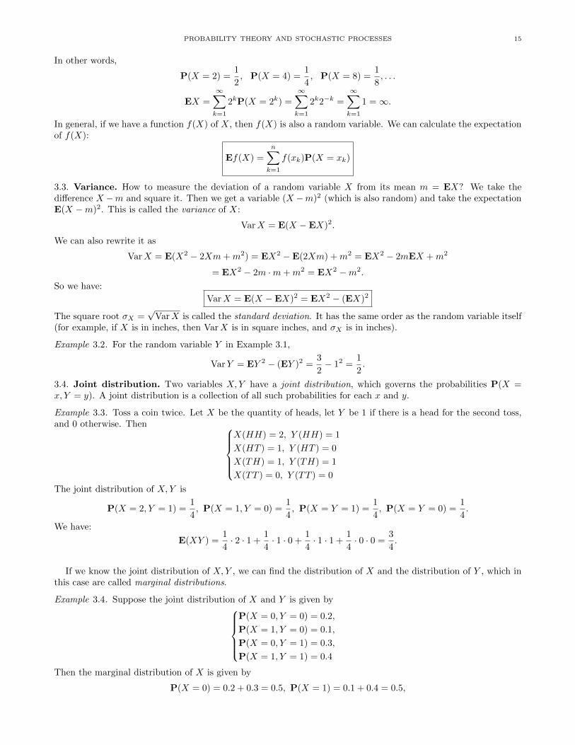
Example 3.4. Suppose the joint distribution of X and Y is given byP(X = 0, Y = 0) = 0.2,

P(X = 1, Y = 0) = 0.1,

P(X = 0, Y = 1) = 0.3,

P(X = 1, Y = 1) = 0.4

Then the marginal distribution of X is given by

P(X = 0) = 0.2 + 0.3 = 0.5, P(X = 1) = 0.1 + 0.4 = 0.5,

16 ANDREY SARANTSEV

and the marginal distribution of Y is given by

P(Y = 0) = 0.2 + 0.1 = 0.3, P(Y = 1) = 0.3 + 0.4 = 0.7.

3.5. Independent random variables. Two discrete random variables X,Y are called independent if

P(X = x, Y = y) = P(X = x) ·P(Y = y)

for all values x and y assumed by X and Y .

Example 3.5. Let X = 1 if the first toss is H, otherwise 0; Y = 1 if the second toss is H, otherwise 0. Then

P(X = 1, Y = 0) =1

4=

1

2

1

2= P(X = 1)P(Y = 0).

Similarly for other values of x and y. So X and Y are independent. But let Z = X + Y . Then X and Z are notindependent. Indeed,

P(X = 1, Z = 2) = P(X = 1, Y = 1) =1

4,

but

P(X = 1) =1

2, P(Z = 2) = P(X = 1, Y = 1) =

1

4

(and 1/4 6= 1/4 · 1/2). Also, X and X are not independent (because it is the same variable!). Indeed,

P(X = 1, X = 1) =1

26= 1

2· 1

2= P(X = 1)P(X = 1).

3.6. Properties of expectation. We always have: E(X + Y ) = EX + EY . For product instead of sum, this isno longer true: E(XY ) 6= EX ·EY . Indeed, let X = Y be the random variable from the example above (result offirst toss). Then

E(XY ) = EX2 =1

2· 12 +

1

2· 02 =

1

2,

but

EX ·EY = (EX)2 = (1/2)2 =1

46= 1

2.

However, for independent random variables, we actually have:

E(XY ) = EX ·EY, if X,Y are independent

Indeed,

E(XY ) =∑x,y

xyP(X = x, Y = y) =∑x,y

xyP(X = x)P(Y = y)

=∑x

xP(X = x)∑y

yP(Y = y) = EXEY.

3.7. Covariance. Random variables X and Y have covariance:

Cov(X,Y ) = E(X −EX)(Y −EY ).

This is a measure of the following: when one variable increases, does the other increase or decrease (on average)?We can also calculate it as

Cov(X,Y ) = E(XY )−EX ·EY.If two variables X and Y are independent, then E(XY ) = EX · EY , and so their covariance is equal to zero:Cov(X,Y ) = 0. For two random variables, if their covariance is positive, they are called positively correlated; if itis negative, they are called negatively correlated. Correlation is defined as

Corr(X,Y ) =Cov(X,Y )√VarX

√VarY

.

It is always between −1 and +1. Such extreme values ±1 show that X and Y are linearly dependent.


Example 3.6. Consider two tosses of a coin. Let X = 1 if the first toss is H, X = 0 otherwise. Z is the quantity ofheads in two tosses. Then

X(HH) = 1, Z(HH) = 2

X(HT ) = 1, Z(HT ) = 1

X(TH) = 0, Z(TH) = 1

X(TT ) = 0, Z(TT ) = 0

Therefore,

E(XZ) =1

4· 1 · 2 +

1

4· 1 · 1 +

1

4· 0 · 1 +

1

4· 0 · 0 =

3

4, EX =

1

2, EZ = 1.

Thus,

Cov(X,Z) =3

4− 1

2· 1 =

1

4.

3.8. Properties of covariance. The following is easy to check:

Cov(X + Y,Z) = Cov(X,Z) + Cov(Y,Z), Cov(X,Y ) = Cov(Y,X), Cov(X,X) = VarX.

Example 3.7. P(X = 0, Y = 0) = 0.5, P(X = 1, Y = 0) = 0.3, P(X = 0, Y = 1) = 0.2. So the distribution of X is

P(X = 0) = 0.7, P(X = 1) = 0.3,

and EX = 0.3. The distribution of Y is

P(Y = 0) = 0.8, P(Y = 1) = 0.2,

and EY = 0.2. Also, always XY = 0, so

Cov(X,Y ) = E(XY )−EXEY = 0− 0.3 · 0.2 = −0.06.

3.9. Properties of variance. Suppose X and Y are random variables. Then

Var(X + Y ) = VarX + VarY + 2 Cov(X,Y )

Indeed,

Var(X + Y ) = E(X + Y −EX −EY )2.

Applying (a+ b)2 = a2 + 2ab+ b2 to a = X −EX and b = Y −EY , we have:

E(X −EX)2 + E(Y −EY )2 + 2E(X −EX)(Y −EY ) = VarX + VarY + 2 Cov(X,Y ).

If X and Y are independent, Cov(X,Y ) = 0 and

Var(X + Y ) = VarX + VarY.

Example 3.8. Toss a coin twice. Let X = 1, if the first toss is heads, and X = 0 otherwise. Let Y = 1 if the secondtoss is heads, Y = 1 otherwise. Then X and Y are independent. So Var(X+Y ) = VarX+VarY = 1/4+1/4 = 1/2.(We calculated VarX = VarY = 1/4 before.)

3.10. Diversification. Suppose you have an asset X which costs now 25; it will bring you 100 or nothing withequal probability. Then

EX =1

2· 100 +

1

2· 0 = 50 > 25.

So it seems to be a good asset. But it has high variance: it is unreliable, and you are likely to lose a lot. A way out:take two such assets X and Y , which are independent (stocks of different companies) and invest equal proportionof your wealth in each asset. You will spend 25, and your return is S = (X + Y )/2, with mean and variance

ES =1

2(EX + EY ) =

1

2(50 + 50) = 50,

VarS =1

22Var(X + Y ) =

1

4(VarX + VarY ) =

1

2VarX.

The variance is twice as small as before. You get the same average return but with low risk. This is calleddiversification; this is essential for finance and insurance. This is why insurance companies need large pools ofclients.

18 ANDREY SARANTSEV

3.11. Modern portfolio theory. This was created by Harry Markowitz in 1952, for which he won a Nobel Prize.Assume we have three assets to invest in, with returns (future price divided by current price) X, Y , Z. Their meanand variance in a year are estimated to be

EX = 3, EY = 2, EZ = 4, and VarX = 2, VarY = 1, VarZ = 4,

and they are independent. How to allocate your funds between these three assets? We need to choose proportionsx, y, z, which satisfy

(1) x, y, z ≥ 0 and x+ y + z = 1.

The return of our portfolio is R = xX + yY + zZ, with

(2) ER = 3x+2y+4z, VarR = Var(xX)+Var(yY )+Var(zZ) = x2 VarX+y2 VarY +z2 VarZ = 2x2+y2+4z2.

Now we need to maximize the return 3x + 2y + 4z given acceptable level of variance: 2x2 + y2 + 4z2 ≤ v, whereyou can choose your v, say v = 1, and given constraints (1). This is done via Lagrange multipliers, which can befound in any optimization textbook. Let us give some examples:

Example 3.9. Equally weighted portfolio: x = y = z = 1/3. Then m = 3 and σ2 = 7/9 = 0.777. Note that thevariance is smaller than for each individual stock. This is the result of our diversification.

Example 3.10. Suppose the investor is risk-averse and invests mostly in the stock Y : x = 0.25, y = 0.5, z = 0.25.Then

m = 3 · 0.25 + 2 · 0.5 + 4 · 0.25 = 2.75,

σ2 = 2 · 0.252 + 0.52 + 4 · 0.252 = 0.625.

In this case, the mean is smaller than for the equally weighted portfolio: 2.75 < 3, but the variance is also smaller:0.625 < 0.777.

But stocks can be also correlated: Assume

corr(X,Y ) = 0.4, and corr(X,Z) = corr(Y, Z) = 0.

Then Cov(X,Y ) = corr(X,Y )√

Var(X) Var(Y ) = 0.4 ·√

2 · 1 =√

20.4. The mean of return is also given by (2),but variance is given by

VarR = Var(xX) + Var(yY ) + Var(zZ) + 2 Cov(xX, yY )

= x2 VarX + y2 VarY + 2xyCov(X,Y ) + z2 VarZ = 2x2 + y2 + 2 ·√

20.4xy + 4z2.

Example 3.11. Equally weighted portfolio: x = y = z = 1/3, and

σ2 = 2 · (1/3)2 + (1/3)2 + 4 · (1/3)2 + 2√

20.4(1/3)2 = 7/9 + 0.8√

2/9.

Variance here is larger than for independent stocks, because of positive correlation.

Problems

For the next eight problems, consider the following setup. Let X be the random number on a die: from 1 to 6.

Problem 3.1. What is the distribution of X?

Problem 3.2. Calculate EX.

Problem 3.3. Calculate EX2.

Problem 3.4. Calculate VarX.


Problem 3.6. Calculate E sin(πX).

Problem 3.7. Calculate E cos(πX).

Problem 3.8. Calculate E(2X − 4).

For the next eleven problems, consider the following setup. Throw a die twice and let X,Y be the results.

Problem 3.9. What is the distribution of X + Y ?

Problem 3.10. Calculate E(X + Y ).

Problem 3.11. Calculate E(2X − 3Y ).


Problem 3.12. Calculate E(XY ).

Problem 3.13. Calculate E(X2Y 2).

Problem 3.14. Calculate Var(X + Y ).

Problem 3.15. Calculate Var(XY ).

Problem 3.16. Find Cov(X,X + Y ).

Problem 3.17. Find Cov(X − Y,X + Y ).

Problem 3.18. Are X and Y independent?

Problem 3.19. Are X and X + Y independent?

Problem 3.20. Toss a fair coin 3 times. Let X be the total number of heads. What is the probability space Ω,and what is the distribution of X?

Problem 3.21. (A game from the Wild West) You bet one dollar and throw three dice. If at least one of them issix, then I return you your dollar and give you as many dollars as the quantity of dice which resulted in six. Forexample, if there are exactly two dice which gave us six, then you win two dollars. If you do not get any dice withsix, then you lose your dollar. So you either lose 1$ or win 1$, 2$ or 3$. What is the expected value of the amountyou win?

Problem 3.22. An urn contains 11 balls, 3 white, 3 red, and 5 blue balls. Take out two balls at random, withoutreplacement. You win $1 for each red ball you select and lose a $1 for each white ball you select. Determine thedistribution of X, the amount you win.

For the next three problems, consider the following setup. An urn contains 10 balls numbered 1, . . . , 10. Select2 balls at random, without replacement. Let X be the smallest number among the two selected balls.

Problem 3.23. Determine the distribution of X.

Problem 3.24. Find EX and VarX.

Problem 3.25. Find P(X ≤ 3).

Problem 3.26. If VarX = 0 and EX = 3, then what can you say about the random variable X?

Problem 3.27. An insurance company determines that N , the number of claims received in a week, is a randomvariable with

P(N = n) =1

2n+1, n = 0, 1, 2, . . . .

The company also determines that the number of claims received in a given week is independent of the number ofclaims received in any other week. Determine the probability that exactly 7 claims will be received during a giventwo-week period.

Problem 3.28. (SOA) The number of injury claims per month is modeled by a random variable N with

P(N = n) =1

(n+ 1)(n+ 2), n = 0, 1, 2, . . .

Determine the probability of at least one claim during a particular month, given that there have been at most fourclaims during that month.

For the next ten problems, consider the following setup. Take two variables: X, Y , with distribution

P(X = −1, Y = 1) = 0.2, P(X = 2, Y = 1) = 0.3,

P(X = −1, Y = 3) = 0.1, P(X = 2, Y = 3) = 0.4.

Problem 3.29. Find the distribution of X.

Problem 3.30. Find the distribution of Y .

Problem 3.31. Calculate EX.

Problem 3.32. Calculate EY .

Problem 3.33. Calculate E(XY ).

20 ANDREY SARANTSEV


Problem 3.35. Calculate VarY .

Problem 3.36. Calculate E(X2Y ).

Problem 3.37. Calculate Cov(X,Y ).

Problem 3.38. Are X and Y independent?

Problem 3.39. (SOA) Let X denote the size of a surgical claim and let Y denote the size of the associated hospitalclaim. An actuary is using a model in which

E(X) = 5, E(X2) = 27.4, E(Y ) = 7, E(Y 2) = 51.4, Var(X + Y ) = 8.

Let C1 = X + Y denote the size of the combined claims before the application of a 20% surcharge on the hospitalportion of the claim, and let C2 denote the size of the combined claims after the application of that surcharge.Calculate Cov(C1, C2).

For the next three problems, consider the following setup. Suppose that ρ is a distribution on −1, 0, 1, withprobabilities 1/3 attached to each of these three numbers. Let X,Y, Z v ρ be i.i.d. random variables.

Problem 3.40. Find E(X + Y + Z).

Problem 3.41. Find E(XY Z).

Problem 3.42. Find P(X = 1 | X + Y + Z = 0).

For the next five problems, consider the following setup. Let X,Y, Z be random variables with the followingjoint distribution:

X Y Z Prob.0 0 0 1/81 0 1 1/80 1 2 1/8−1 1 1 1/83 1 0 1/2

Problem 3.43. Find the distribution and the expectation of each of these three random variables.

Problem 3.44. Find Cov(X,Y ).

Problem 3.45. Find the distribution of XY + Z.

Problem 3.46. Calculate E(X + 1)4.

Problem 3.47. Calculate E(XY Z).

Problem 3.48. Toss a fair coin 3 times. Let X,Y be numbers of Heads and Tails. Find Cov(X,Y ).

Problem 3.49. Find the distribution of XY − Z for random variables X,Y, Z with joint distribution

X Y Z Prob.2 1 0 0.50 1 −1 0.31 0 −2 0.2

Problem 3.50. (SOA) A car dealership sells 0, 1, or 2 luxury cars on any day. When selling a car, the dealer alsotries to persuade the customer to buy an extended warranty for the car. Let X denote the number of luxury carssold in a given day, and let Y denote the number of extended warranties sold. We have:

P(X = 0, Y = 0) =1

6, P(X = 1, Y = 0) =

1

12, P(X = 2, Y = 0) =

1

12,

P(X = 1, Y = 1) =1

6, P(X = 2, Y = 1) =

1

3, P(X = 2, Y = 2) =

1

6.

Calculate the variance of X.

Problem 3.51. Consider two random variables X and Y with joint distribution

P(X = −1, Y = 0) = P(X = 1, Y = 0) = P(X = 0, Y = 1) = P(X = 0, Y = −1) =1

4.

Are they independent? Find Cov(X,Y ).


Problem 3.52. Consider a random variable X with distribution

P(X = −1) = 0.4, P(X = 0) = 0.4, P(X = 1) = 0.2

Find its expectation and the standard deviation.

Problem 3.53. Two independent random variables X and Y have joint distribution

P(X = 2, Y = 0) =1

2, P(X = 2, Y = 1) =

1

4, P(X = 1, Y = 0) = p, P(X = 1, Y = 1) = q.

Find p and q.

Problem 3.54. Toss a fair coin three times. Let X be the number of Heads during the first two tosses. Let Ybe the number of Tails during the last two tosses. For example, if the sequence of tosses is TTH, then X = 0 andY = 1. Are X and Y independent? Why or why not?

For the next six problems, consider the following setup. Toss a fair coin twice and let X be the number of Heads,and let Y = 1 if the first toss is Tails, Y = 0 otherwise. Find:

Problem 3.55. The distribution of X.

Problem 3.56. The distribution of Y .

Problem 3.57. EX.

Problem 3.58. VarX.

Problem 3.59. Cov(X,Y ).

Problem 3.60. P(X = 2 | Y = 0).

For the next four problems, we have a portfolio of 4 stocks, the first and the second of which have returns withmean 1 and variance 2, and the third and the fourth have returns with mean 1.2 and variance 3. For each setup,find the mean and variance of the return.

Problem 3.61. All returns are independent, equally-weighted portfolio.

Problem 3.62. All returns are independent, portfolio which invests equally in the first three stocks.

Problem 3.63. Correlation between the first two stocks is −0.8, all other correlations are zero, equally-weightedportfolio.

Problem 3.64. Correlation between the second and the third stock is 0.5, all other correlations are zero, portfoliowhich invests 30% in each of the first two stocks, and 20% in the last two stocks.

Problem 3.65. We invest in 10 independent assets, each has return with mean 1 and variance 7. Find the meanand variance of the equally-weighted portfolio.

Problem 3.66. We invest in 50 independent assets, 20 of which have returns with mean 0.4 and variance 1, 30 ofwhich have returns with mean 0.5 and variance 1.4. Find the mean and variance for the equally-weighted portfolio.

Problem 3.67. We invest in N independent assets, each has return with mean 1 and variance 2. For which N dowe have the variance of the equally-weighted portfolio less than or equal to 0.1?

4. Common Discrete Distributions

4.1. Bernoulli distribution. Suppose you have a biased coin, which falls H with probability p, 0 < p < 1. Youtoss it once. Let X = 1 if the first toss resulted in H, X = 0 if the first toss resulted in T. Therefore, the distributionof X is

P(X = 1) = p, P(X = 0) = q = 1− p.This is called a Bernoulli distribution with probability of success p. We can calculate its expectation and variance:

EX = 1 · p+ 0 · q = p, EX2 = 12 · p+ 02 · q = p,

VarX = EX2 − (EX)2 = p− p2 = p(1− p) = pq.

22 ANDREY SARANTSEV

4.2. Binomial distribution. Suppose you have a biased coin, which falls H with probability p, 0 < p < 1. Youtoss it N times. Let X be the number of H. What is the distribution of the random variable X? We call this thesequence of Bernoulli trials: each trial can independently result in success (H) or failure (T), with probabilities pand q = 1 − p respectively. Let X1 = 1 if the first toss resulted in H, X1 = 0 if the first toss resulted in T. Samefor X2, X3, . . . . Then

X = X1 +X2 + . . .+XN

The random variables X1, . . . , XN are Bernoulli, independent and identically distributed (i.i.d.): P(Xi = 1) =p, P(Xi = 0) = q. What is the probability that X = k? Let us consider the extreme cases: all H or all T.

P(X = 0) = qN , P(X = N) = pN .

Now, consider the case of general k. We can choose which k tosses out of N result in H, there are(Nk

)choices.

Each choice has probability pkqN−k. So

P(X = k) =

(N

k

)pkqN−k, k = 0, . . . , N

We denote the distribution of X by Bin(N, p): binomial distribution with parameters N and p, or sequence of NBernoulli trials with probability p of success. We write: X v Bin(N, p). Let us calculate the expectation andvariance of the binomial distribution:

EX = EX1 + . . .+ EXN = p+ p+ . . .+ p = N.

Since X1, . . . , XN are independent, we have:

VarX = VarX1 + . . .+ VarXN = pq + . . .+ pq = Npq.

Example 4.1. Toss twice a biased coin, when the probability of Heads is p = 2/3. The number of Heads isX v Bin(2, 2/3). Therefore,

P(X = 0) = P(TT ) =1

3· 1

3=

1

9,

P(X = 1) = P(TH,HT ) = P(TH) + P(HT ) =1

3· 2

3+

2

3· 1

3=

4

9,

or, alternatively,

P(X = 1) =

(2

1

)(1

3

)1(2

3

)1

= 2 · 1

3· 2

3=

4

9,

and, finally,

P(X = 2) = P(HH) =2

3· 2

3=

4

9.

4.3. Poisson distribution. Fix a parameter λ > 0. Consider a distribution on 0, 1, 2, 3, . . ., given by the formula

P(X = k) =λk

k!e−λ, k = 0, 1, 2, . . .

This is called the Poisson distribution with parameter λ. We write: X v Poi(λ). For example,

P(X = 0) = e−λ, P(X = 1) = λe−λ, P(X = 2) =λ2

2e−λ, P(X = 3) =

λ3

6e−λ.

Recall the Taylor series for exponential function:

ex = 1 + x+x2

2+x3

6+ . . . =

∞∑k=0

xk

k!.

This means that∞∑k=0

P(X = k) =

∞∑k=0

λk

k!e−λ = e−λ

∞∑k=0

λk

k!= e−λeλ = 1.

And it should be so, since for a probability distribution, all individual probabilities should sum up to 1. What isEX for X v Poi(λ)?

EX =

∞∑k=0

k ·P(X = k) =

∞∑k=0

k · λk

k!e−λ =


(because the term corresponding to k = 0 is zero, so we can omit it from the sum)

=

∞∑k=1

kλk

k!e−λ =

(because k/k! = 1/(k − 1)!)

=

∞∑k=1

λk

(k − 1)!e−λ =

∞∑m=0

λm+1

m!e−λ = λ

∞∑m=0

λm

m!e−λ = λ.

This proves that

EX = λ

After calculation, we can also show that

VarX = λ

4.4. Approximation theorem. Consider a binomial distribution Bin(N, p). If N → ∞, and Np = λ, thenBin(N, p)→ Poi(λ). More precisely, for every fixed k = 0, 1, 2, . . ., we have as N →∞:(

N

k

)pkqN−k → λk

k!e−λ.

Proof. Note that p = λ/N , q = 1− λ/N , and(N

k

)=

N !

k!(N − k)!=N(N − 1) . . . (N − k + 1)

Nk.

Therefore, (N

k

)pkqN−k =

N(N − 1) . . . (N − k + 1)

Nk

(λ

N

)k (1− λ

N

)N−k=λk

k!· N(N − 1) . . . (N − k + 1)

Nk·(

1− λ

N

)N−k.

The first factor λk/k! is constant (does not depend on N); the second factor is

N(N − 1) . . . (N − k + 1)

Nk=N

N· N − 1

N· . . . · N − k + 1

N→ 1,

because each of these fractions tends to one: indeed, N →∞, and k is fixed. Finally, the third factor tends to e−λ,because

log

(1− λ

N

)N−k= (N − k) log

(1− λ

N

)v (N − k)

(− λN

)= −λN − k

N→ −λ,

and then we exponentiate both sides. We use the tangent line approximation:

log(1 + x) v x, x→ 0,

which is true: let f(x) = log(1 + x); then f ′(x) = 1/(1 + x), and so f(0) = 0, f ′(0) = 1, and

f(x) v f(0) + f ′(0)x = x, x→ 0.

This is the meaning of a Poisson distribution: this is approximately the quantity of many events, each of whichis very rare.

Example 4.2. A company which sells flood insurance has N = 20000 clients, and each client has probability offlood p = 0.01%, independently of others. What is the distribution of the number X of floods? Approximately itis X v Bin(N, p), but it is hard for calculations: for example,

P(X = 10) =

(20000

10

)(1

10000

)10(9999

10000

)19990

.

Use Poisson approximation: X is approximately distributed as Poi(2), because λ = Np = 2. So

P(X = 10) =210

10!e−2.

Also,P(X ≥ 3) = 1−P(X = 0)−P(X = 1)−P(X = 2)

24 ANDREY SARANTSEV

= 1− e−2 − 21

1!e−2 − 22

2!e−2 = 1− e−2 − 2e−2 − 2e−2 = 1− 5e−2.

4.5. Poisson paradigm. A slightly more general statement is true. If we have N (a large number of) independentevents, occuring with probabilities p1, . . . , pN , then the quantity of events which happened is approximately Poi(λ)with λ = p1 + . . .+ pN .

So the Poisson distribution is the law of rare events: if we have many events, each of which is very unlikely tooccur, then the number of events is Poisson.

Example 4.3. A company which sells flood insurance has three groups of clients. The first group, N1 = 10000, islow-risk: each client has probability p1 = 0.01% of a flood, independently of others. The second group, N2 = 1000clients, is medium-risk: p2 = 0.05%. The third group, N3 = 100 clients, is high-risk, p3 = 0.5%. For every flood,a company pays 100, 000$. How much should it charge its clients so that is does not go bankrupt with probabilityat least 95%?

The quantity X of floods is Poisson with parameter

λ = N1p1 +N2p2 +N3p3 = 2.

Let us find k such that P (X ≤ k) ≥ 95%: after calculation (possibly using the histogram), you can find that k = 5.So we will have at most 5 floods with high probability, and the company will pay no more than 500, 000$ with highprobability. This sum should be taken from clients in the form of premuims. But we would like to charge high-riskclients more. Also, the company needs to cover its costs of operation and get some profit, so the real change willbe greater than 500, 000$.

4.6. Geometric distribution. Toss a biased coin, with probability p of Heads, and probability q = 1−p of Tails.How many X tosses do you need to get your first Heads? This is called geometric distribution with parameter p,and denotes X v Geo(p), meaning that X has geometric distribution with parameter p. For example, if we havethe sequence of tosses TTTHTHH, then X = 1. We have:

P(X = n) = P(TT . . . T︸︷︷︸n−1

H) = pqn−1, n = 1, 2, 3, . . . .

We can alternatively describe it as the number of Bernoulli trials you need to get your first success. 1 Let uscalculate:

EX =

∞∑n=1

npqn−1.

Take a function

f(x) =

∞∑n=1

pxn = px(1 + x+ x2 + . . .) =px

1− x ; f ′(q) =

∞∑n=1

pnqn−1 = EX.

But we can calculate f ′(q):

f ′(x) =px′(1− x)− p(1− x)′x

(1− x)2=p(1− x) + px

(1− x)2=

p

(1− x)2,

and so f ′(q) = p/(1− q)2 = p/p2 = 1/p. This proves that

EX =1

p

The meaning of this is commonsensical: if you have success with probability, say, 1/4, then you need, on average,four trials to get success. Similarly, we can find that

VarX =q

p2

1Sometimes the geometric distribution is defined as the number of T, rather than tosses, to get your first H. This shifts it by 1.

Then it takes values 0, 1, 2, . . . In these lectures, we assume that Geometric distribution is the number of tosses until your first H.


4.7. Negative binomial distribution. How many times X do you need to toss a coin to get r Heads, where r isa fixed parameter? This is called negative binomial distribution NB(r, p). For example, if r = 3 and the sequenceis TTTHTHH, then X = 7. What is P(X = n)? If the nth toss resulted in rth Heads, another way to say this isthe first n− 1 tosses contain r− 1 Heads and n− r Tails, and the last, nth toss resulted in Heads. The probabilitythat the first n− 1 tosses resulted in r − 1 Heads (and n− r Tails) is(

n− 1

r − 1

)pr−1qn−r.

Indeed, there are (n− 1

r − 1

)choices for slots in the first n−1 tosses occupied by Heads. Each of these choices has probability pr−1qn−r. Finally,the probability of the last toss being Heads is p. So

P(N = n) =

(n− 1

r − 1

)prqn−r

This is true for n = r, r+1, r+2, . . .. The random variable X v NB(r, p) can take only values greater than or equalto r, because to get r Heads, you need at least r tosses. One can alternatively describe this distribution as thenumber of Bernoulli trials one needs to get to the rth success. For r = 1, this becomes the Geometric distributionwith parameter p. 2

Example 4.4. Let p = 1/2, r = 2. Then

P(X = 3) =

(3− 1

2− 1

)(1

2

)2(1− 1

2

)= 2 · 1

4· 1

2=

1

4.

We can equivalently get this as follows: to get two Heads in exactly three tosses, we need either THH or HTH.Each of these sequences has probability 1/8. So the resulting probability is (1/8) + (1/8) = 1/4.

For X v NB(r, p), we have:

X = X1 + . . .+Xr, X1, . . . , Xr v Geo(p) i.i.d.

Recall that i.i.d. means independent identically distributed. Indeed, to get to the rth Heads, we need to get thefirst Heads, which required geometric number X1 of tosses; then we need to get from first to second Heads, whichrequired also geometric number X2 of tosses. This second number is independent of the first one, because the coindoes not have a memory, etc. Therefore,

EX = EX1 + . . .+ EXr =r

p,

and using independence, we get:

VarX = VarX1 + . . .+ VarXr =qr

p2.

The negative binomial distribution and the binomial distribution answer somewhat opposite questions. For thebinomial distribution, you have fixed number of tries, and you ask how many successful trials you have. For thenegative binomial distribution, you have fixed number of successful trials, and you ask how many trials you need.

Problems

Problem 4.1. Find P(X ≤ 4) for X v Bin(3, 0.7).

Problem 4.2. Find P(X ≤ 4) for X v Bin(5, 0.7).

Problem 4.3. Find P(X ≤ 4) for X v Poi(1).

Problem 4.4. In a family with four children, how likely is the even split (two boys, two girls)? Solve this problemif there are 1.05 boys for every girl (real data for USA).

Problem 4.5. For X v Bin(10, 0.1), calculate P(X = 1) in a direct way and using Poisson approximation.Compare the results. Calculate the relative error, which is (x − a)/a, where a is the exact value and x is theapproximation.

2Similarly to the geometric distribution, there is ambiguity in the definition of the negative binomial distribution. Sometimes itis defined as the quantity of T, as opposed to tosses, until your first H. In this case, it is shifted by r down. Thus defined negative

binomial random variable takes values 0, 1, 2, . . . We define this distribution as the number of tosses until your rth H.

26 ANDREY SARANTSEV

Problem 4.6. The monthly worldwide number of airplane crashes averages λ = 3. Assuming that it has a Poissondistribution, find the probability that there will be at least one crash. If it already occurred this month, what isthe probability that there will be at least one more?

Problem 4.7. (SOA) A baseball team has scheduled its opening game for April 1. If it rains on April 1, the gameis postponed and will be played on the next day that it does not rain. The team purchases insurance against rain.The policy will pay 1000 for each day, up to 2 days, that the opening game is postponed. The insurance companydetermines that the number of consecutive days of rain beginning on April 1 is a Poisson random variable withmean 0.6. What is the standard deviation of the amount the insurance company will have to pay?

Problem 4.8. (SOA) A study is being conducted in which the health of two independent groups of ten policyholdersis being monitored over a one-year period of time. Individual participants in the study drop out before the end ofthe study with probability 0.2 (independently of the other participants). What is the probability that at least 9participants complete the study in one of the two groups, but not in both groups?

Problem 4.9. (SOA) A tour operator has a bus that can accommodate 20 tourists. The operator knows thattourists may not show up, so he sells 21 tickets. The probability that an individual tourist will not show up is0.02, independent of all other tourists. Each ticket costs 50, and is non-refundable if a tourist fails to show up. Ifa tourist shows up and a seat is not available, the tour operator has to pay 100 (ticket cost + 50 penalty) to thetourist. What is the expected revenue of the tour operator?

Problem 4.10. Find P(X ≤ 2) for X v Geo(1/2).

Problem 4.11. Find P(X ≤ 5) for X v NB(3, 1/3).

Problem 4.12. Find P(X ≥ 3) for X v NB(3, 1/3).

Problem 4.13. Find P(X = 0) for X v Geo(1/4).

Problem 4.14. For a random variable X ∼ NB(2016, 0.25), find P(X ≤ 2017).

Problem 4.15. There areN = 1000 houses, each is on fire independently of other houses with probability p = 0.4%.Find the probability that there are exactly six fires.

Problem 4.16. The amount of loss in a car accident has geometric distribution with parameter 1/3. An insurancecompany applies a deductible of 2, which means the following. If the amount of loss is less than or equal to 2,then the customer pays out of his pocket and the company pays nothing. If the amount of loss exceeds 2, then thecustomer pays the first 2 and the company pays the rest. Given that the company has to pay something greaterthan zero, what is the probability that it pays 1?

Problem 4.17. Throw a die three times and let X be the quantity of even-numbered results: 2, 4 or 6. Throwit three more times and let Y be the quantity of the dice (among the last three dice, not the total of six dice)which are equal to 6. For example, if we have the sequence 364656 of six dice, then X = 2 and Y = 2. CalculateVar(X − Y ).

Problem 4.18. You take five preliminary exams, and you will pass each exam with probability 1/3, independentlyof other exams. What is the probability that you will pass two or more exams?

Problem 4.19. Take a sequence of independent Bernoulli trials, each has probability p = 0.4 of success. Let Xbe the number of trials you need to get to your first success. Find E(2X + 3)2.

Problem 4.20. There are N = 100 clients, each will experience flood with probability p = 0.5%, independently ofothers. What is the probability that exactly one client will experience flood? (Hint: use Poisson approximation.)

Problem 4.21. Suppose you throw a die and say that you have success if you get 5 or 6. You want to get twosuch successes. What is the probability that you need exactly 10 tries for this? (Which means that your 10th trywill bring you the second success.)

Problem 4.22. A company sells car insurance. There are two types of drivers: N1 = 5000 good drivers, andN2 = 3000 bad drivers. This year, each good driver gets into an accident with probability p1 = 0.01%, and eachbad driver gets into an accident with probability p2 = 0.03%. All accidents can happen independently of oneanother. Find approximately the probability that there will be at least two accidents this year.

Problem 4.23. Suppose you take a sequence a Bernoulli trials with probability p = 0.4 of success. Let X be thenumber of trials you need to make to get 4 successful trials. Find EX and VarX.


Problem 4.24. Toss six fair coins. Let X be the number of Heads in the first two tosses. Let Y be the numberof Tails in the last four tosses. Find E(X − Y ) and Var(X − Y ).

Problem 4.25. An insurance company sells car insurance, with an obligation to pay 100, 000$ in case of anaccident. There are four caterogies of people:

• teenagers: N1 = 1500, p = 0.05%;• young adults with college education: N2 = 2000, p = 0.01%;• young adults without college education: N3 = 1500, p = 0.03%;• middle-aged people: N4 = 3000, p = 0.02%.

The first number refers to the quantity of people in each category. The second number refers to the probability ofan accident for a given person in this category. The company wants to pay all the claims using money collectedfrom premiums. It wants to be able to do this with probability 90% or more. What is the amount of money itshoud collect?

Problem 4.26. (SOA) A company buys a policy to insure its revenue in the event of major snowstorms that shutdown business. The policy pays nothing for the first such snowstorm of the year and 10000 for each one thereafter,until the end of the year. The number of major snowstorms per year that shut down business is assumed to have aPoisson distribution with mean 1.5. Calculate the expected amount paid to the company under this policy duringa one-year period.

Problem 4.27. There are N1 = 1000 high-risk clients, each of whom can have an accident with probabilityp1 = 0.06%, and N2 = 1000 low-risk clients, each of whom can have an accident with probability p2 = 0.03%. Allaccidents occur independently. Given that the number of accidents is less than 3, find the probability that thereare no accidents.

Problem 4.28. A client has losses X ∼ Geo(0.6). The insurance policy has a deductible of 3: if the losses are 3or less, the company does not pay anything, while if the losses are greater than 3, the company pays 80% of thedifference. Find the expected value of the payment.

5. Continuous Random Variables

5.1. Continuous distributions. A random variable X has continuous distribution with density p(x) if for everya and b

P(a ≤ X ≤ b) =

∫ b

a

p(x) dx.

Unlike discrete random variables, this one takes any fixed value with probability zero: P(X = a) = 0. The density

must satisfy p(x) ≥ 0 and∫ +∞−∞ p(x) dx = 1. We compute the expectation as

EX =

∫ +∞

−∞xp(x) dx.

Indeed, split the curve p(x) into small sections [x, x+ dx]. The probability of X falling into each section is p(x) dx.This section corresponds to the value X = x. Sum these up; since these quantities are infinitesimal, you will obtainthe integral above. You can also view it as a continuous analogy of the formula

EX =∑x

x ·P(X = x)

for discrete random variables. Similarly,

Ef(X) =

∫ +∞

−∞f(x)p(x) dx

Example 5.1. Consider the density

p(x) =

cx, 0 ≤ x ≤ 1;

0, else.

Let us find the constant c > 0: since the density must integrate up to 1, we have:∫ 1

0

cxdx = 1 ⇒ c

∫ 1

0

xdx =1

2c = 1 ⇒ c = 2.

28 ANDREY SARANTSEV

Next, we can find expectation and variance:

EX =

∫ +∞

−∞xp(x) dx = 2

∫ 1

0

x2 dx =2

3,

EX2 =

∫ +∞

−∞x2p(x) dx = 2

∫ 1

0

x3 dx =1

2,

VarX = EX2 − (EX)2 =1

2−(

2

3

)2

=1

18

5.2. Examples of continuous distributions. There are three main classes of continuous distributions which weshall study: Normal (Gaussian), Gamma, and Uniform. Here, we shall provide densities for the Standard Normal(a particular case of Normal), Exponential (a particular case of Gamma), and Uniform.

1. Standard Normal, or Gaussian. X v N (0, 1). It has the ”bell curve” density

p(x) =1√2πe−x

2/2

The coefficient 1/√

2π isnecessary to make this density integrate up to 1, because one can show that∫ +∞

−∞e−x

2/2 dx =√

2π.

2. Exponential. X v Exp(λ) (parameter λ > 0) if

p(x) =

λe−λx, x ≥ 0;

0, x < 0.

We sometimes say: exponential with mean λ−1, because EX = 1/λ. The parameter λ is called the rate. 3

3. Uniform on [c, d]. X v Uni[c, d] if

p(x) =

1d−c , c ≤ x ≤ d;

0, for other x.

5.3. Expectation and variance of the standard normal distribution. Assume X v N (0, 1). Then

EX =

∫ +∞

−∞xe−x

2/2 dx = 0,

because the function inside the integral is odd. We can also say that X is symmetric with respect to zero, soEX = 0. Now,

EX2 =1√2π

∫ +∞

−∞x2e−x

2/2 dx = 1.

Why is this? We know that ∫ +∞

−∞e−x

2/2 dx =√

2π.

Let u = e−x2/2, v = x. Integrate by parts: note that uv = xe−x

2/2 = 0 for x = ±∞. So∫ +∞

−∞e−x

2/2 dx =

∫ +∞

−∞udv = uv|x=+∞

x=−∞ −∫ +∞

−∞v du

= −∫ +∞

−∞xde−x

2/2 = −∫ +∞

−∞x (−x)e−x

2/2 dx =

∫ +∞

−∞x2e−x

2/2 dx.

This is equal to√

2π, which proves EX2 = 1. So VarX = EX2 − (EX)2 = 1. This proves that

X ∼ N (0, 1) ⇒ EX = 0, VarX = 1

3 Sometimes the exponential distribution is parametrized using the mean: Exp(β) means the distribution with density on the

positive half-line: p(x) = β−1e−x/β , for x > 0. Then β = λ−1 = EX. In our lectures, we use the parametrization with rate λ.


5.4. Normal distribution with general parameters. If X v N (0, 1), we say that Y = µ + σX v N (µ, σ2).This random variable has EY = µ+ σEY = µ and VarY = σ2 VarX = σ2. Therefore, it is called normal randomvariable with mean µ and variance σ2. Its density is given by

p(y) =1√2πσ

exp

(− (y − µ)2

2σ2

)Indeed,

P(a ≤ Y ≤ b) = P(a ≤ µ+ σX ≤ b) = P

(a− µσ≤ X ≤ b− µ

σ

)=

1√2π

(b−µ)/σ∫(a−µ)/σ

e−x2/2 dx.

Now let us change variables:

x =y − µσ

; dx =dy

σ; a ≤ y ≤ b.

Therefore,

1√2π

(b−µ)/σ∫(a−µ)/σ

e−x2/2 dx =

1√2πσ

b∫a

e−(y−µ)2/(2σ2) dy =

∫ b

a

p(y) dy.

This proves that Y has density p(y), as shown above.

Example 5.2. For X ∼ N (1, 4), find E[(X − 2)3

]: X = 1 + 2Z with Z ∼ N (0, 1), and (X − 2)3 = (2Z − 1)3 =

8Z3 − 12Z2 + 6Z − 1. Taking the expected value and using EZ = EZ3 = 0 (by symmetry of the standard normal

distribution), EZ2 = 1, we get: E[(X − 2)3

]= −12− 1 = −13

5.5. Cumulative distribution function and quantiles. The cumulative distribution function (CDF) of a ran-dom variable X is

F (x) = P(X ≤ x) =

∫ x

−∞p(y) dy.

For some random variables, such as exponential and uniform, it can be explicitly calculated. For other variables,such as normal, it cannot be calculated in an exact form. But it is tabulated, see the Z-table for X ∼ N (0, 1) atthe end.

Example 5.3. Calculate the CDF of X ∼ Exp(2). For x ≤ 0, we have: F (x) = 0, because X ≥ 0 always. For x > 0,

we have: F (x) =∫ x

02e−2x dx = (−e−2x)

∣∣x=∞x=0

= 1− e−2x. Therefore,

F (x) =

0, x ≤ 0;

1− e−2x, x ≥ 0.

Example 5.4. For X ∼ N (1, 4), find P(X ≤ 3): X = 1 + 2Z with Z ∼ N (0, 1), and P(X ≤ 3) = P(1 + 2Z ≤ 3) =P(Z ≤ 1) = 0.8413

An α-quantile of a distribution of X is a number x such that P(X ≤ x) = α. Quantiles of the standard normaldistribution are given in the Z-table, see the end of these lecture notes. They are denoted as xα.

Example 5.5. Find x, the 95% quantile of X ∼ Exp(2):

P(X ≤ x) = 0.95 ⇔ 1− e−2x = 0.95 ⇔ e−2x = 0.05 ⇔ x = −1

2ln(0.05) = 1.50

Example 5.6. Find a normal distribution with mean 1 and 99% quantile 4.5. We can represent this random variableas X = 1 + σZ, where σ needs to be found. Because

0.99 = P(X ≤ 4.5) = P(1 + σZ ≤ 4.5) = P(Z ≤ σ−13.5),

from the Z-table at the end of these lecture notes we get: σ−13.5 = x99% = 2.326, so σ = 3.5/2.326 = 1.505, and

X ∼ N (1, 1.505)

30 ANDREY SARANTSEV

5.6. Lognormal distribution. If X v N (µ, σ2) is a normal random variable, then we say that the randomvariable Y = eX has lognormal distribution. The meaning of this is as follows: a normal variable X models thesum X1 + . . .+XN of many independent random variables (the Central Limit Theorem). And a lognormal randomvariable Y = eX models their product X1 . . . XN . This is indeed true, because

log(X1 . . . XN ) = logX1 + logXN ≈ X,

so

X1 . . . XN ≈ eX = Y.

Sometimes in real life an observed variable is the sum of many small factors (for example, the total vote for eachcandidate is the sum of individual votes). But in other situations, this observed variable is the product of smallfactors, such as height of a person. In this case, it is a good idea to model this variable by a lognormal distribution.Let us find the density of this lognormal distribution. The density of the normal distribution N (µ, σ2) is given by

p(x) =1√2πσ

exp

(− (x− µ)2

2σ2

).

Therefore,

P(a ≤ Y = eX ≤ b) = P(log a ≤ X ≤ log b) =

∫ log b

log a

1√2πσ

exp

(− (x− µ)2

2σ2

)dx

Now, let us make a change of variables:

x = log y, dx =dy

y, log a ≤ x ≤ log b ⇒ a ≤ y ≤ b.

We have:

P(a ≤ Y ≤ b) =

∫ b

a

1√2πσy

exp

(− (log y − µ)2

2σ2

)dy.

Therefore, the density of the lognormal distribution is

p(y) =1√

2πσyexp

(− (log y − µ)2

2σ2

).

5.7. Transformations of continuous random variables. We can apply similar technique to find density ofY = f(X), where X is a given continuous random variable, and f is a one-to-one function (that is, to every y thereis no more than one x such that f(x) = y). Best to illustrate this with the following example: let X ∼ Exp(2), andf(x) = x2. Then for the random variable Y = f(X) = X2, for any positive a and b, we have:

P(a ≤ Y ≤ b) = P(a1/2 ≤ X ≤ b1/2

)=

∫ b1/2

a1/22e−2x dx.

Now make change of variable x = y1/2, then

a1/2 ≤ x = y1/2 ≤ b1/2 ⇒ a ≤ y ≤ b, dx =1

2y−1/2 dy.

Then the integral takes the form∫ b

a

2e−2y1/2 1

2y−1/2 dy =

∫ b

a

p(y) dy, where p(y) := y−1/2e−2y.

Therefore, we represented the probability

P(a ≤ Y ≤ b) =

∫ b

a

p(y) dy.

Thus, p(y) is the density of Y .


5.8. Properties of exponential distribution. Consider X v Exp(λ), exponential distribution with parameterλ > 0. It has density

p(x) =

λe−λx, x ≥ 0;

0, x < 0.

We sometimes say: exponential with mean λ−1, because after calculations:

EX =

∫ ∞0

λxe−λx dx =

∫ ∞0

xd(−e−λx

)=

= x ·(−e−λx

)∣∣x=∞x=0

−∫ ∞

0

(−e−λx

)dx = 0− 0 +

∫ ∞0

e−λxdx = − 1

λ

∫ ∞0

d(−e−λx

)=

− 1

λ

(−e−0 − (−e−∞)

)=

1

λ.

We also have: for a > 0,

P(X ≥ a) =

∫ ∞a

λe−λx dx =(−e−λx

)∣∣x=∞x=a

= e−λa.

The exponential distribution has memoryless property: for s, t > 0,

P(X > t+ s | X > s) = P(X > t).

Indeed,

P(X > t+ s | X > s) =P(X > t+ s,X > s)

P(X > s)=

P(X > t+ s)

P(X > s)=e−λ(s+t)

e−λs= e−λt = P(X > t).

Sometimes exponential distribution is used to model the lifespan of a device, when the remaining lifespan isindependent of how long it has worked so far.

5.9. Power laws. This is density p(x) = cx−α−1 for x ≥ x0. It integrates to one, therefore∫ ∞x0

p(x) dx = 1 ⇒ cx−α0

α= 1.

This is sometimes called Pareto law, or heavy tails: because probabilities P(X ≥ x) for large x are much largerthan for exponential or normal distributions with same mean and variance.

Example 5.7. p(x) = 0.5x−1.5, x ≥ 1. Then the mean is infinite:

EX =

∫ ∞1

xp(x) dx = 0.5

∫ ∞1

x−0.5 dx = cx0.5

0.5

∣∣∣∣x=∞

x=1

=∞.

Example 5.8. p(x) = cx−2.5, x ≥ 2. Here, c can be found from the total integral:

1 =

∫ ∞2

cx−2.5 dx = cx−1.5

−1.5

∣∣∣∣∞x=2

= c2−1.5

1.5⇒ c = 1.5 · 21.5 = 3

√2.

Then the mean is finite:

EX =

∫ ∞2

xp(x) dx = c

∫ ∞2

x−1.5 dx = cx−0.5

−0.5

∣∣∣∣x=∞

x=2

= c2−0.5

0.5= 6,

but the second moment (and therefore the variance) is infinite:

EX2 =

∫ ∞2

x2p(x) dx = c

∫ ∞2

x−0.5 dx = cx0.5

0.5

∣∣∣∣∞x=2

=∞.

32 ANDREY SARANTSEV

5.10. Independence for continuous distributions. Two random variables X and Y are called independent iffor every subsets A and B we have:

P(X ∈ A, Y ∈ B) = P(X ∈ A) ·P(Y ∈ B).

We cannot formulate the definition as

P(X = x, Y = y) = P(X = x) ·P(Y = y),

because the probability that X takes a given value is zero! For continuous random variables, expectation andvariance have the same properties as for discrete ones. For all random variables X and Y ,

E(X + Y ) = EX + EY, Cov(X,Y ) = E(XY )− (EX)(EY ),

Var(X + Y ) = VarX + VarY + 2 Cov(X,Y ).

For independent random variables X and Y ,

E(XY ) = (EX)(EY ), Cov(X,Y ) = 0, Var(X + Y ) = VarX + VarY.

5.11. Mixtures. It is not true that all distributions are either discrete or continuous. Assume a client has anaccident with probability 10%, and the losses are distributed as X ∼ Exp(2). We have:

EX = 0.5, VarX = 0.25 ⇒ EX2 = (EX)2 + VarX = 0.5.

Then the amount Z of losses is a random variable which has distribution

P(Z = 0) = .9, P(a < Z < b) = .1 ·∫ b

a

2e−2x dx.

This is a mixture of two distributions, one concentrated at 0 and the other exponential, with weights 0.9 and 0.1respectively. Then

EZ = .9 · 0 + .1 ·EX = .05,EZ2 = .9 · 02 + .1 ·EX2 = 0.05.

Therefore, VarZ = EZ2− (EZ)2 = 0.05− 0.052. We can also have mixtures of continuous distributions (which arethemselves continuous).

Example 5.9. Take a random variable Z, which is a mixture of X ∼ Exp(0.5) and Y ∼ N (2, 1) with weights 75%and 25% respectively.4 Recall that

EX =1

0.5= 2, EY = 2, EX2 = VarX + (EX)2 =

1

0.52+

(1

0.5

)2

= 8, EY 2 = VarY + (EY )2 = 5.

The random variable Z has density

pZ(x) = 0.75pX(x) + 0.25pY (x) =

0.75 · 0.5e−0.5x + 0.25 · 1√

2πe−(x−1)2/2, x ≥ 0;

0.25 · 1√2πe−(x−1)2/2, x < 0.

Its expectation and variance are

EZ = 0.75EX + 0.25EY = 0.75 · 2 + 0.25 · 2 = 2

EZ2 = 0.75EX2 + 0.25EY 2 = 0.75 · 8 + 0.25 · 5 = 7.25

and therefore VarZ = EZ2 − (EZ)2 = 7.25− 22 = 3.25

4Do not confuse Z with W = 0.75 ·X + 0.25 · Y , which is not a mixture of distributions.


5.12. Joint density. Random variables X and Y have joint density p(x, y) if for every subset C ⊆ R2, we have:

P((X,Y ) ∈ C) =

∫∫C

p(x, y) dA.

For example,

P(X ∈ A, Y ∈ B) =

∫A

∫B

p(x, y) dy dx.

If X and Y are independent, then the joint density

p(x, y) = pX(x)pY (y)

is the product of densities pX of X and pY of Y . In the general case (if they are not independent), the marginaldensity of X can be reconstructed as follows:

pX(x) =

∫ +∞

−∞p(x, y) dy.

Indeed, because for all a and b we have:

P(a ≤ X ≤ b) = P(a ≤ X ≤ b,−∞ < Y < +∞) =

∫ b

a

∫ +∞

−∞p(x, y) dy dx,

then the expression∫ +∞−∞ p(x, y) dy plays the role of density for X. Similarly,

pY (y) =

∫ +∞

−∞p(x, y) dx

is the marginal density of Y . The expectation of X is given by

EX =

∫xpX(x)dx =

∫ ∫xp(x, y) dxdy,

and the expectation of f(X,Y ) is given by

Ef(X,Y ) =

∫∫f(x, y)p(x, y) dxdy

Example 5.10. Suppose p(x, y) = x+ y, if 0 ≤ x, y ≤ 1, and 0 otherwise. Then

pX(x) =

∫ 1

0

(x+ y)dy =

(xy +

y2

2

)∣∣∣∣y=1

y=0

= x+1

2.

EY =

∫ 1

0

∫ 1

0

(x+ y)y dx dy =

∫ 1

0

∫ 1

0

(xy + y2) dy dx =

∫ 1

0

(xy2

2+y3

3

)∣∣∣∣y=1

y=0

dx

=

∫ 1

0

(1

2x+

1

3

)dx =

1

2

x2

2

∣∣∣∣x=1

x=0

+1

3x|x=1x=0 =

1

4+

1

3=

7

12

E(XY ) =

∫ 1

0

∫ 1

0

(xy)(x+ y)dxdy = . . . = calculate

Example 5.11. Suppose p(x, y) = 2e−x−2y, x, y > 0. Then this joint density can be represented in the productform:

p(x, y) = pX(x)pY (y), pX(x) = e−x, pY (y) = 2e−2y.

Therefore, X ∼ Exp(1) and Y ∼ Exp(2) are independent.

Example 5.12. Consider two continuous random variables (X,Y ) distributed uniformly on the triangle (x, y) ∈R2 | 0 ≤ x ≤ 1, 0 ≤ y ≤ x. That is, their joint density is equal to

p(x, y) =

2, 0 ≤ x ≤ 1, 0 ≤ y ≤ x;

0, else.

Let us find EY 2. We have:

EY 2 =

∫ 1

0

∫ x

0

2y2 dy dx =

∫ 1

0

2y3

3

∣∣∣∣y=x

y=0

dx =

∫ 1

0

2

3x3 dx =

2

3· x

4

4

∣∣∣∣x=1

x=0

=1

6

34 ANDREY SARANTSEV

5.13. Convolution. Suppose X and Y are independent discrete random variables, taking values 0, 1, 2, . . .. Thenthe distribution of X + Y can be calculated as follows:

P(X + Y = n) =

n∑k=0

P(X = k)P(Y = n− k), n = 0, 1, 2, . . .

If X and Y take values 0,±1,±2, . . . (negative as well as positive), then

P(X + Y = n) =

∞∑k=−∞

P(X = k)P(Y = n− k), n = 0,±1, . . .

Example 5.13. Take X ∼ Poi(λ) and Y ∼ Poi(µ). Then

P(X + Y = n) =

n∑k=0

λk

k!e−λ

µn−k

(n− k)!e−µ =

e−λ−µ

n!

n∑k=0

λkµn−kn!

k!(n− k)!=e−λ−µ

n!(λ+ µ)n.

Therefore, X + Y ∼ Poi(λ+ µ).

For continuous random variables X and Y , if they are nonnegative, with densities pX and pY , we have: thedensity of X + Y is given by

pX+Y (x) =

∫ x

0

pX(y)pY (x− y) dy, x ≥ 0.

If X and Y are not necessarily nonnegative, then

pX+Y (x) =

∫ ∞−∞

pX(y)pY (x− y) dy.

This is called convolution of pX and pY .

5.14. Gamma distribution. Take X,Y ∼ Exp(λ). Then pX(x) = pY (x) = λe−λx, and

pX+Y (x) =

∫ x

0

λe−λy · λe−λ(x−y)dy = λ2

∫ x

0

e−λxdy = λ2xe−λx, x ≥ 0.

Next, X,Y, Z ∼ Exp(λ), then

pX+Y+Z(x) =

∫ x

0

pX+Y (y)pZ(x− y)dy =

∫ x

0

λ2ye−λy · λe−λ(x−y)dy = λ3e−λx∫ x

0

ydy = λ3x2

2e−λx.

More generally, the sum of n i.i.d. Exp(λ) random variables has density

p(x) =λn

(n− 1)!xn−1e−λx.

This distribution is called Gamma distribution Γ(n, λ). For n = 1, we are back to Exp(λ). 5 We changed variablesy = λx, so that λαxα−1dx = yα−1dy. Let us find expectation and variance of X ∼ Γ(n, λ): we can represent X as

X = X1 + . . .+Xn, Xi ∼ Exp(λ) i.i.d.

Therefore, because EXi = λ−1 and VarXi = λ−2, we have:

(3) EX = EX1 + . . .+ EXn =n

λ, VarX = VarX1 + . . .+ VarXn =

n

λ2.

Example 5.14. Find the density of X ∼ Γ(4, 3), as well as EX and EX2. The density is given by

p(x) =34

(4− 1)!x4−1e−3x =

34

6x3e−3x =

27

2x3e−3x.

EX =4

3, VarX =

4

32⇒ EX2 = (EX)2 + VarX =

16

9.

5Similarly to the exponential distribution, sometimes the Gamma distribution is parametrized via β := λ−1. We use λ.


5.15. Gamma distribution for non-integer parameter. We can generalize it for non-integer n as follows.Define the notion of generalized factorial, or Gamma function. Note that

n! = In :=

∫ ∞0

xne−xdx.

Why? Integrate In by parts:

(4) In = −∫ ∞

0

xnde−x = − xne−x∣∣x=∞x=0

+

∫ ∞0

e−xd (xn) = 0 + n

∫ ∞0

xn−1e−xdx = nIn−1.

Combining that with I0 =∫∞

0e−xdx = 1, we have: In = n!. Thus, define for α > 0:

α! :=

∫ ∞0

xαe−xdx.

Usually, we talk about the Gamma function, defined for all α > 0:

Γ(α) = (α− 1)! =

∫ ∞0

xα−1e−xdx.

Similarly to (4), we get

(5) Γ(α+ 1) = αΓ(α), α > 0.

Example 5.15. Let us find Γ(1/2) = (−1/2)!: we can change variables x = u2/2 in the following integral

(6) Γ(1/2) =

∫ ∞0

x−1/2e−x dx.

Then we have: dx = udu, and x−1/2 dx =√

2u−1 · udu =√

2 du. Thus, the integral in (6) can be written as

√2

∫ ∞0

e−u2/2 du =

√2√

2π

∫ ∞0

e−u2/2

√2π

du = 2√π · 1

2=√π

Example 5.16. Find Γ(5/2): From (5) we get that

Γ(5/2) = (3/2)Γ(3/2) = (3/2)(1/2)Γ(1/2) =3

4

√π

Define the Gamma distribution Γ(α, λ):

p(x) =λα

Γ(α)xα−1e−λx, x > 0.

For α = 1, we are back to Exp(λ). This is indeed a probability distribution, because it integrates to 1:∫ ∞0

p(x)dx =1

Γ(α)

∫ ∞0

yα−1e−ydy =Γ(α)

Γ(α)= 1.

We changed variables y = λx, so that λαxα−1dx = yα−1dy. Note that the expectation and variance are given bythe same formulas as in (3), with n changed to α. We shall show this in Section 8.

Example 5.17. Find the density of the Gamma distribution with mean 2 and variance 4. We have:

α

λ= 5,

α

λ2= 10.

Dividing the first equation over the second, we get: λ = 0.5, and α = 5λ = 2.5. Therefore, the density is given by

0.52.5

Γ(2.5)x1.5e−0.5x =

0.52.5

3√π/4

x1.5e−0.5x = 3

√2

πx1.5e−x/2

36 ANDREY SARANTSEV

5.16. Service life. Let us model the distribution of the remaining time of service of a certain device. Let T beits (random) lifetime. Assume this is a continuous random variable, with density p(t) and cumulative distribution

function F (t) = P(T ≤ t) =∫ t

0p(s) ds. Then S(t) = P(T ≥ t) = 1− F (t) is called survival function, and

f(t) =p(t)

S(t)=F ′(t)

S(t)= −S

′(t)

S(t)= −(lnS(t))′

is called the failure rate. If a device still works by time t, that is T ≥ t, then for small dt we have:

P(T ≤ t+ dt | T ≥ t) =P(t ≤ T ≤ t+ dt)

P(T ≥ t) =p(t) dt

S(t)= f(t) dt.

That is, among N such devices by time t, approximately Nf(t) dt will fail during time [t, t + dt]. The simplestmodel is with constant failure rate f(t) = λ. This gives us exponential distribution:

−(lnS(t))′ = λ ⇒ lnS(t) = lnS(0)− λt = −λt ⇒ S(t) = e−λt.

We used S(0) = 1: all devices still work at time t = 0. Other models take into account rising failure rate: say,f(t) = A+Be−Ct or f(t) = A+BtC for some constants A,B,C > 0.

Problems

Problem 5.1. (SOA) The loss due to a fire in a commercial building is modeled by a random variable X withdensity function

f(x) =

0.005(20− x), 0 < x < 20;

0, otherwise.

Given that a fire loss exceeds 8, what is the probability that it exceeds 16?

Problem 5.2. (SOA) In a small metropolitan area, annual losses due to storm, fire, and theft are assumed tobe independent, exponentially distributed random variables with respective means 1.0, 1.5, 2.4. Determine theprobability that the maximum of these losses exceeds 3.

Problem 5.3. For X ∼ N (−2, 2), find EX3.

Problem 5.4. For X ∼ N (3, 4), find E[(X2 − 1)2

].

Problem 5.5. For X ∼ N (−1, 3), find E[(X + 1)3

].

Problem 5.6. For X ∼ N (−2, 2), find P(−3 ≤ X ≤ 0).

Problem 5.7. For X ∼ N (3, 4), find P(X ≥ 4 | X ≥ 3).

Problem 5.8. Find a normal distribution with mean −1 and 95% quantile equal to 2.3

Problem 5.9. Find a normal distribution with 1% quantile at −3.4 and 99% quantile at 2.4.

Problem 5.10. Find a normal distribution with standard deviation 2.5 and 5% quantile at −15.2.

Problem 5.11. Find an exponential distribution such that P(Z ≥ 3) = 0.4.

Problem 5.12. Find the cumulative distribution function of Z − 3, where Z ∼ Exp(0.5).

Problem 5.13. Find an exponential distribution with P(X ≥ 4 | X ≥ 3) = 0.5.

Problem 5.14. Find the parameters of the gamma distribution with mean 4 and variance 4/3.

Problem 5.15. (SOA) An actuary models the lifetime of a device using the random variable Y = 10X0.8, whereX is an exponential random variable with mean 1 year. Determine the probability density function f(y), for y > 0,of the random variable Y .

Problem 5.16. (SOA) A device runs until either of two components fails, at which point the device stops running.The joint density function of the lifetimes of the two components, both measured in hours, is

p(x, y) =1

8(x+ y) , 0 ≤ x ≤ 2 and 0 ≤ y ≤ 2.

Calculate the probability that the device fails during its first hour of operation.

Problem 5.17. For a random variable X with density cex, 0 ≤ x ≤ 2, find the constant c and find EeX .


Problem 5.18. An insurance company insures a large number of homes. The insured value X of a randomlyselected home follows a distribution with density function

f(x) =

2x−3, x ≥ 1;

0, otherwise.

Given that a home is insured for at least 2, find the probability it is insured for less than 3.

Problem 5.19. Calculate EX3 and EX4 for X v N (0, 1). For EX4, use the same trick as for EX2 in the lecture:

integration of x2e−x2/2 by parts, u = x2e−x

2/2, v = x. (See lecture notes, Section 5.)

Problem 5.20. For a random variable X ∼ Uni[0, 1], find the density of logX.

Problem 5.21. For a random variable X ∼ Exp(3), find the density of 2X2.

Problem 5.22. (SOA) Two random variables X and Y have joint density121 (x+ y), 1 ≤ x ≤ 3, 0 ≤ y ≤ 3;

0, otherwise.

Find the probability P(X ≥ 2, Y ≤ 2).

Problem 5.23. Calculate EX and VarX for X v Uni[c, d].

Problem 5.24. Let X ∼ N (−1, 4), Y ∼ Γ(5, 2) be independent random variables. Find Var(Y − 2X − 3).

Problem 5.25. For X with density p(x) = 3x2, 0 ≤ x ≤ 1, find EX3.

Problem 5.26. Find coefficients a and b such that for independent X ∼ N (0, 1) and Y ∼ N (1, 2) we have:aX + bY ∼ N (3, 21).

Problem 5.27. Find EY 2 for two continuous random variables (X,Y ) distributed uniformly on the triangle(x, y) ∈ R2 | 0 ≤ x ≤ 1, 0 ≤ y ≤ x. That is, their joint density is equal to

p(x, y) =

2, 0 ≤ x ≤ 1, 0 ≤ y ≤ x;

0, else.

Problem 5.28. (SOA) Calculate the expected value for a continuous random variable with density function:

f(x) =

|x|/10, −2 ≤ x ≤ 4;

0, otherwise.

Problem 5.29. (SOA) A manufacturer’s annual losses follow a distribution with density function

f(x) = 2.5(0.6)2.5x−3.5, x > 0.6,

and f(x) = 0 otherwise. To cover its losses, the manufacturer purchases an insurance policy with an annualdeductible of 2. Calculate the mean of the manufacturer’s annual losses not paid by the insurance policy.

Problem 5.30. (SOA) An insurance policy covers a loss X ∼ Uni[0, 1000]. Calculate the deductible d such thatthe expected payment under the policy with deductible is 25% of what it would be with no deductible.

Problem 5.31. (SOA) Let X and Y be continuous random variables with joint density function

f(x, y) =8

3xy, 0 ≤ x ≤ 1, x ≤ y ≤ 2x,

and f(x, y) = 0 otherwise. Calculate Cov(X,Y ).

Problem 5.32. Two-thirds of auto insurance clients are teenagers, who have losses distributed exponentially withmean 5, and the other third are middle-aged people, who have losses distributed exponentially with mean 1. Findthe density, mean, and variance of the distribution of losses for a random client.

For the next four problems, consider a client has an accident with probability 20%, and the losses are distributedexponentially with mean 10. Let X be the total amount of losses.

Problem 5.33. Find VarX.

Problem 5.34. Find EX3.

Problem 5.35. Find P(X ≤ 2).

38 ANDREY SARANTSEV

Problem 5.36. Find P(1 < X < 3).

For the next three problems, let X have a mixture of two distributions: Bin(4, .4) and N (0, 2), with weights 0.3and 0.7.

Problem 5.37. Find EX and VarX.

Problem 5.38. Find P(2 ≤ X ≤ 3).

Problem 5.39. Find P(X = 0 | X ≤ 2).

Problem 5.40. For independent X ∼ N (3, 2), Y ∼ N (−1, 4), Z ∼ N (0, 1), find P(−X + 2Y − Z ≤ 3).

Problem 5.41. The failure rate for a device is f(t) = 1 + 2t. If it is time 2 and it is still serving, what is theprobability it will serve at least 3 more units of tme?

Problem 5.42. A device has two parts, and it works as long as both parts work. Each part has constant failurerate, 2 for the first part and 3 for the second part. Find the service time distribution and failure rate for the wholedevice.

Problem 5.43. The failure rate for a device is f(t) = 3 + 2t5/2. Write down, but do not evaluate, the integral forthe mean service time.

Problem 5.44. We know that Γ(α, β) has mean 2 and standard deviation√

5. Find α, β.

Problem 5.45. Find the density of 3X4 if X is exponential with mean 2.

Problem 5.46. Find the density of X + Y , where X ∼ Γ(3, 2) and Y ∼ Γ(5, 2) are independent.

For the next five problems, consider (X,Y ) with density p(x, y) = 24xy, 0 ≤ x, y; x+ y ≤ 1.

Problem 5.47. Find EX.

Problem 5.48. Find VarY .

Problem 5.49. Find corr(X,Y ).

Problem 5.50. Find E(X2Y ).

Problem 5.51. Find P(X ≤ 0.5 | Y ≥ 0.5).

Problem 5.52. For X with p(x) = x−2, x ≥ 1, find EX and P(X ≤ 2).

Problem 5.53. For X with p(x) = 2x−3, x ≥ 1, find EX and VarX.

Problem 5.54. For x with p(x) = cx−3.5, x ≥ 3, find c, EX, VarX.

6. Central Limit Theorem

6.1. Statement for IID variables. Suppose X1, X2, X3, . . . are iid (independent identically distributed) randomvariables with mean EX1 = EX2 = . . . = µ and variance VarX1 = VarX2 = . . . = σ2. Consider the sum

SN := X1 + . . .+XN .

Note that

ESN = EX1 + . . .+ EXN = µN, VarSN = VarX1 + . . .+ VarXN = σ2N.

The last equation used that X1, X2, . . . are independent. Therefore, for every N the random variable

SN −ESN√VarSN

=SN − µNσ√N

has mean zero and variance 1. As N →∞, we have:

SN − µNσ√N

→ N (0, 1)

Here N (0, 1) is the standard normal distribution. A random variable X is distributed according to N (0, 1): X vN (0, 1), if

P(a ≤ X ≤ b) =1√2π

∫ b

a

e−x2/2 dx.


This convergence means that, as N →∞,

P

(a ≤ SN − µN

σ√N

≤ b)→ 1√

2π

∫ b

a

e−x2/2 dx,

for every real numbers a, b. We cannot compute the antiderivative∫e−x

2/2 dx as an elementary function. So thereare tables of the normal distribution, in print and online (just Google them). If Xk has Bernoulli distribution:

P(Xk = 1) = p, P(Xk = 0) = q, p+ q = 1,

then µ = EXk = 1 · p+ 0 · q = p, and (after calculation) VarXk = σ2 = pq.

Example 6.1. Suppose we have a plane of N = 200 people. Each customer, independently of others, chooses chickenor pasta, with probability 50%. How many chicken and pasta is needed to satisfy chicken-lovers with probability95% and pasta-lovers with probability 95% (so that everybody will be satisfied with probability 90%)?

If we prepare only 100 chicken and 100 pasta, we will likely run out ofeither chicken or pasta: it is very unlikelythat exactly 100 people will choose chicken. The other extreme is to prepare 200 chicken and 200 pasta. Thisguarantees that every client will be pleased, but a lot of food (200 meals) will be thrown away. Which is not good,because airlines have tight budgets. Let us find a compromise. Let Xk = 1 if the kth person chooses chicken,Xk = 0 if he chooses pasta. Then SN = X1 + . . . + XN is the total number of chicken required. The randomvariable Xk is Bernoulli, with p = 1/2, so

µ =1

2, σ2 =

1

4, σ =

1

2;

SN −Nµσ√N

=SN − 100√

200/2≈ N (0, 1).

We can find x95% = 1.645 such that

Φ(x) =1√2π

∫ x

−∞e−u

2/2 du = 95%.

Therefore, approximately

P

(SN − 100√

200/2≤ 1.645

)≈ 95%.

With this high probability 95%,

SN − 100√200/2

≤ 1.645 ⇔ SN ≤ 100 +1

2

√200 · 1.645 = 112.

So we need only 112 chicken: 100 chicken according to the mean, and 12 additional, as a buffer. The same appliesto pasta. We will throw away 12 + 12 = 24 meals after the trip, which is not a lot. Or maybe just give them topilots or flight attendants.

6.2. Normal and Poisson approximations. Suppose you have a large quantity N of independent events, each ofwhich happens with probability p. The number of these events is Bin(N, p). We have studied two approximations:

• Poisson, when Bin(N, p)→ Poi(λ) if p = λ/N , as N →∞.• Normal, when for X v Bin(N, p), as N →∞, for constant p (independent of N):

X − pN√pqN

→ N (0, 1).

The first approximation is used when the events are rare, the second - when they are ”usual”, not rare. In practice,if you have something like N = 1000 and p = 0.1%, you should use Poisson, and if N = 1000 but p = 10%, youshould use Normal.

6.3. Equity buffer, or value at risk. An insurance company has N clients. The kth client has insurance claimXk. Suppose X1, X2, X3, . . . are iid (independent identically distributed) random variables with mean EX1 =EX2 = . . . = µ and variance VarX1 = VarX2 = . . . = σ2. The sum

SN := X1 + . . .+XN

is the total amount the company has to cover. How much should it charge clients so that it is not bankrupt withprobability α (close to 1, say 95%)? By Central Limit Theorem,

SN − µNσ√N

≈ N (0, 1).

40 ANDREY SARANTSEV

Therefore, if xα is such that

Φ(xα) =1√2π

∫ xα

−∞e−y

2/2 dy = α,

then with probability (approximately) α, we have:

SN − µNσ√N

≤ xα ⇔ SN ≤ µN + σ√N · xα = VaRα .

The value VaRα is called equity buffer, or value at risk, corresponding to the level of confidence α. The companyshould accumulate this amount in premiums (=money which clients pay for coverage), or using money from othersources, to be able to fulfil its obligations with probability α. Suppose that the company splits this sum betweenclients evenly: this makes sense, because clients pose the same risk (which is another way to say that X1, X2, . . .are identically distributed). Then each client pays the premium (cost of the policy)

1

NVaRα = µ+

1√Nσxα.

This premium consists of two parts: µ, which is net premium, covering the average risk, and the overhead 1√Nσxα,

which covers risk. Indeed, it makes sense for an insurance company to demand at least the average of expectedpayoff as a premuim. But this is not enough, because the company bears clients’ risk. The company has the rightto demand additional payment, which is the overhead.

Note also that the larger N is, the smaller the overhead is. This is called economies of scale: companies need todiversify risks among a large pool of clients; the larger this pool is, the better.

6.4. Extensions of the Central Limit Theorem. The CLT (central limit theorem) is valid not only for iid(independent identically distributed) random variables. It is (sometimes) true if variables are independent but notidentically distributed, or if they have slight dependence. The search for the conditions under which CLT is validis still an active research area. For the purposes of this class, you can assume it is true if VarSN is large. This ishow it is formulated in the general form.

SN −ESN√VarSN

→ N (0, 1), N →∞

Example 6.2. An insurance company has N1 = 10000 clients, each with claim Geo(1/2), and N2 = 40000 clients,each with claim Geo(2/3). What is the value at risk for confidence level 95%?

Let Xk be the claim of the kth client from the first group, and let Yk be the claim of the kth client from thesecond group. Then the total amount of claims is

S = S50000 = X1 + . . .+XN1 + Y1 + . . .+ YN2 .

Let us calculate ES and VarS. Recall the expectation and variance for geometric distribution:

EXk =1

1/2= 2, VarXk =

1− 1/2

(1/2)2= 2, EYk =

1

2/3=

3

2, VarYk =

1− 2/3

(2/3)2=

3

4.

Therefore,

ES = 2 ·N1 +3

2·N2 = 80000, VarS = 2 ·N1 +

3

4·N2 = 50000.

By the CLT, we have:S − 80000√

50000≈ N (0, 1).

Therefore, the following inequality is true with probability approximately 95%:

S − 80000√50000

≤ 1.645 ⇔ S ≤ 80000 +√

50000 · 1.645.

The value at risk is 80000 +√

50000 · 1.645

Example 6.3. There are N = 1000000 (one million) eligible voters; each votes with probability p = 49% for Smithand with probability q = 51% for Johnson. Votes of different voters are independent. What is the probability thatSmith wins? We assume all voters do vote. Let Xk = 1, if kth voter votes for Smith, Xk = 0 otherwise. Then

SN = X1 + . . .+XN


is the number of votes for Smith. Smith wins if SN > N/2. But P(Xk = 1) = p, P(Xk = 0) = q, so EXk = p = µand VarXk = pq = σ2. By the CLT, we have:

SN − pN√pqN

≈ N (0, 1).

Therefore,

P(SN > N/2) = P

(SN − pN√

pqN>N/2− pN√

pqN

)= P

(N (0, 1) >

N/2− pN√pqN

).

ButN/2− pN√

pqN=

(1/2− 0.49) · 1000000√0.49 · 0.51 · 1000000

≈ 20.

Therefore,

P(SN > N/2) = P(N (0, 1) > 20) =1√2π

∫ ∞20

e−y2/2 dy < 10−50.

Almost certainly, Johnson will win. Smith does not have any chance.

Problems

Problem 6.1. An insurance company has N = 10000 clients. Each of them can get into a car accident withprobability 10%, independently of each other. If a client gets into a car accident, the amount of the claim is 1000dollars. The company charges each of them a premium x. Calculate the minimal amount of x so that the companygets bankrupt only with probability 5%.

Problem 6.2. An insurance company has N = 10000 clients. Half of them file a claim which is distributed asExp(1). The other half file a claim Exp(2); all claims are independent. Find the probability that the total amountwill be between 7400 and 7560.

Problem 6.3. A health insurance company has three types of clients: low-risk, medium-risk, and high-risk. Thereare N1 = 10000 low-risk clients, each will have a claim which is exponential with mean 100; N2 = 3000 medium-riskclients, each will have a claim which is exponential with mean 200; and N3 = 1000 high-risk clients, each will havea claim which is exponential with mean 1000. All claims are independent of each other. Find the value at risk forconfidence level 99%.

For the next three problems, suppose you have N independent events, each of which has probability p. Will yourather use Normal or Poisson appoximation for the number of these events, if:

Problem 6.4. N = 1000 and p = 0.2%.

Problem 6.5. N = 10000 and p = 30%.

Problem 6.6. N = 4000 and p = 0.01%.

Problem 6.7. (SOA) An insurance company issues 125 vision care insurance policies. The number of claims filedby a policyholder under a vision care insurance policy during one year is a Poisson random variable with mean 24.Assume the numbers of claims filed by different policyholders are mutually independent. Calculate the approximateprobability that there is a total of between 3000 and 3100 claims during a one-year period.

Problem 6.8. There are two candidates for the local government office: Richard Hunter and Mary Williams. Eachvoter chooses Richard and Mary independently of other voters, with probability 49% and 51% respectively. Thereare N = 100 voters. What is the chance that Richard pulls out an upset victory?

Problem 6.9. An insurance company has N = 10000 clients. Each of them files a claim with size Poi(3),independently of others. Find the value at risk for the confidence level 99%: how much money the company needsto collect to be able to pay all claims with probability 99%.

Problem 6.10. Each of N = 50000 car owners will get into an accident independently with probability eitherp1 = 1% (high-risk drivers, 10000 of them) or p2 = .5% (low-risk drivers, 40000 of them). What is the probabilitythat the number of accidents will differ from the mean by at least 10%?

Problem 6.11. A financial analyst models 10-year returns of 500 stocks from the Standard & Poor 500 index asindependent random variables with mean 3.5 and variance 3.2. This analyst then invests into an equally weightedportfolio, so the return of this portfolio is equal to the average of these returns. Which normal distribution modelsthe return of this portfolio? What is the probability that the actual return will be below 3?

42 ANDREY SARANTSEV

Problem 6.12. An insurance company wants to charge its N clients a premium which corresponds to overhead20%, that is, 20% higher than the average loss of this client. Each client sustains a loss of 250 or 100 withprobabilities 10% and 20%, respectively. The company wants to be able to pay with probability 98%. What is theminimal number N of clients?

For the next two problems, there are N = 10000 car drivers. Each gets into an accident with probability 15%.In case of an accident, the losses are distributed uniformly on [0, 10]. Assume independence.

Problem 6.13. Find the probability that the total losses exceed 8000.

Problem 6.14. Find the value at risk at the confidence level 95%.

7. Introduction to Statistics

7.1. Estimation. Consider iid (independent identically distributed) random variables X1, . . . , XN with (unknown)mean and variance

µ = EX1 = EX2 = . . . = EXN , σ2 = VarX1 = VarX2 = . . . = VarXN .

We want to estimate µ and σ2. The estimate for µ: empirical mean

(7) x =X1 + . . .+XN

N.

The estimate for σ2:

(8) s2 =1

N − 1

N∑k=1

(Xk − x)2.

Why do we divide by N − 1, as opposed to N? Because it makes the estimate unbiased: Es2 = σ2.Good estimates should satisfy two properties:

• Unbiased: the expected value of the estimate should be equal to the true value of parameter. Here, it isindeed true:

Ex =1

N(EX1 + . . .+ EXN ) =

1

N(µ+ . . .+ µ) = µ.

• Consistent: as the number of observations tends to infinity, an estimate should converge to the true valueof the parameter it is trying to estimate. This is indeed true by the Law of Large Numbers:

x→ µ, N →∞.The estimate s2 of σ2 also satisfies these properties: it is unbiased, and consistent (harder to prove).If we have two jointly distributed random variables (X,Y ), then their covariance Cov(X,Y ) can be estimated

from a sample of i.i.d. (x1, y1), . . . , (xN , yN ) as follows:

(9) Q =1

N − 1

N∑k=1

(xk − x)(yk − y).

This estimate is also unbiased and consistent.

7.2. Confidence intervals. Suppose you are trying to find not a precise estimate, but an interval of values inwhich the parameter likely lies. Let α be the level of confidence, say 95%. What is the confidence interval for µ?By the Central Limit Theorem,

X1 + . . .+XN − µNσ√N

≈ N (0, 1).

Therefore, let us find x97.5% such that

P (N (0, 1) ≤ x97.5%) =1√2π

∫ x97.5%

−∞e−t

2/2 dt = 97.5%.

We split the bell curve into three parts: the right tail, which is 2.5%, the left tail, which is also 2.5%, and themiddle, which is 95%. Therefore, with probability 95%,

−x97.5% ≤X1 + . . .+XN − µN

σ√N

≤ x97.5%.

−x97.5%σ√N

≤ X1 + . . .+XN − µNN

= x− µ ≤ x97.5%σ√N

.


Rewrite this as

−x97.5%σ√N

+ x ≤ µ ≤ x97.5%σ√N

+ x.

This is the confidence interval for µ. If you do not know σ, then substitute s from s2. Note that the confidenceinterval gets smaller as n grows. But it is larger if you set a higher confidence level.

Example 7.1. Assume we take observations X1, . . . , XN ∼ N (θ, 9) for N = 10000 and are trying to estimate theunknown parameter θ. Let us find a confidence interval for the level of confidence 10%. Assume that x = 1.4353.Then the confidence interval is given by(

−x95%

√9√

10000+ 1.4353,

x95%

√9√

10000+ 1.4353

)= (−0.04935 + 1.4353, 0.04935 + 1.4353).

7.3. Hypotheses testing. Suppose you want to test the hypothesis µ = 0 at level of confidence 95% (or, whichis the same, for p = .05).

Then we construct the confidence interval for α = 95% and find whether µ = 0 lies in this interval. If it doesnot, then we reject this hypothesis with confidence level 95%, or with p = .05. Because if we accept this hypothesis,then an unlikely event (with probability 5%) happened. If µ = 0 does lie in this interval, then we do not reject thishypothesis, because it is still consistent with the experiment.

Example 7.2. A hotly debated Proposition X is on the polls for the local town referendum during this electionseason. A local newspaper polls N1 = 100 people and 53 of them say they support Proposition X. Next week,another poll of N2 = 100 people finds that 57 of them support Proposition X. The paper has a headline: ”Supportfor Proposition X grows”. You are unconvinced and would like to test the hypothesis that the level of supportremained unchanged: 53%, since the last week. Let us test this for confidence level p = 90%.

The hypothesis says that each vote is distributed as a Bernoulli random variable with p = 0.53. This distributionhas mean µ = p = 0.53 and variance σ2 = p(1− p) = 0.53 · 0.47 = 0.2491. Therefore, we should check whether

−x0.95%σ√N2

+ µ ≤ x ≤ x0.95%σ√N2

+ µ.

If this is true, then we do not reject the hypothesis that each vote is distributed as a Bernoulli random variable withp = 0.53 (that is, support for Proposition X has not changed). If this is false, then we do reject this hypothesis. Itturns out that

1.645 ·√

0.2491√100

+ 0.53 = 0.08 + 0.53 = 0.61 > 0.57 = x,

and, of course,

1.645 ·√

0.2491√100

+ 0.53 = 0.53− 0.08 = 0.45 < 0.57.

Therefore, we do not reject the hypothesis p = 0.53.

7.4. Bayesian methods. These methods for confidence intervals and hypotheses testing were developed by Fisher.However, these Fisherian methods are sometimes inappropriate, because p is arbitrary, and because they testhypotheses without taking into account our prior beliefs in them. Bayesian methods aim to correct this disadvantageby using Bayes’ theorem to switch from prior probabilities to posterior probabilities.

Suppose there is a poll of N = 100 people, with 53 expressing support for Proposition X. What is the actuallevel of support? Assume we have three hypotheses:

H1 : p = 40%; H2 : p = 50%; H3 : p = 60%.

Let us test these hypotheses for confidence level p = 90%. As in the previous subsection, we reject the hypothesisH1, but do not reject the hypotheses H2 and H3. Now, suppose you beileved prior to this poll that

P(H1) = 50%, P(H2) = 30%, P(H3) = 20%.

How shall you update your beliefs after the poll? Let A be the event that this poll happened. By Bayes’ formula,

P(H1 | A) =P(A | H1)P(H1)

P(A | H1)P(H1) + P(A | H2)P(H2) + P(A | H3)P(H3).

However,

P(A | H1) =

(100

53

)0.4530.647, P(A | H2) =

(100

53

)0.5530.547, P(A | H3) =

(100

53

)0.6530.447.

44 ANDREY SARANTSEV

Thus, after calculations, you get the following posterior probabilities:

P(H1 | A) = 4.7%, P(H2 | A) = 73.7%, P(H3 | A) = 21.5%.

If another poll is conducted, then you again update your probabilities. This is the method Nate Silver uses in hisblog FiveThirtyEight to predict presidential and other elections.

Problems

For the next five problems, consider the following setup. You have N = 100 observations, with x = 3.56 ands2 = 18.24.

Problem 7.1. Find the confidence interval for the confidence level α = 90%.

Problem 7.2. Find the confidence interval for α = 95%.

Problem 7.3. For what confidence level can we reject the hypothesis that µ = 3.5?

Problem 7.4. Same question for µ = 3.6.

Problem 7.5. Same question for µ = 4.

Problem 7.6. Assume you estimate the rate parameter λ for Exp(λ) by estimating the mean λ−1. Your N = 200observations give you x = 0.545 and s2 = 0.2533. Find an estimate for λ and the confidence interval for λ withconfidence level α = 98%.

For the next five problems, consider the following setup. There are two candidates: Richard Hunter and MaryWilliams. A poll of N = 1500 voters shows 733 supporting Richard, and 867 supporting Mary.

Problem 7.7. How likely is it that Richard wins?

Problem 7.8. Can you reject this hypothesis at the confidence level 95%?

Problem 7.9. What is the confidence interval for the share of vote for Mary at level 98%?

Problem 7.10. Assume we have initially three hypotheses: the share of Mary’s support is 25%, 50%, and 75%,with prior probabilities 20%, 60%, and 20%, respectively. What are posterior probabilities for each hypothesis?

Problem 7.11. Assume we have initially two hypotheses: the share of Mary’s support is 40% and 60%, with priorprobabilities 65% and 35%, respectively. What are posterior probabilities for each hypothesis?

For the next three problems, consider the following setup. Proposition A is on the ballot. A poll of N = 200people finds that 112 of them support A. A week later, another poll of M = 250 people finds that 134 of themsupport A.

Problem 7.12. Can we reject the hypothesis that the support remains unchanged, with confidence level 95%?

Problem 7.13. Judging by the second poll, can we reject the hypothesis that A will fail, at confidence level 95%?

Problem 7.14. Assume you have the following hypotheses for the share of support: p = 50%, p = 60%, p = 40%,with prior probabilities 50%, 25%, 25%. What are the posterior probabilities after the first poll? After the firstand second poll?

Problem 7.15. Find the estimates x and s2 for the selection 0, 1, 2, . . . , N .

8. Generating and Moment Generating Functions

8.1. Generating functions. Take a random variable X which takes values 0, 1, 2, . . . It has a generating function:

ϕX(s) := EsX =

∞∑k=0

P(X = k)sk.

We can do this only for random variables taking values in the nonnegative integers, not with negative or fractionalvalues, or continuous distributions. If you know this generating function, you know all values pk := P(X = k) foreach k = 0, 1, 2, . . ., and so you know the distribution of X. Note that always ϕX(1) = E1X = E1 = 1.

For a Poisson random variable: X ∼ Poi(λ), we have:

P(X = k) =λk

k!e−λ, k = 0, 1, 2, . . . ,


and therefore

ϕX(s) =

∞∑k=0

λk

k!e−λsk = e−λ

∞∑k=0

(sλ)k

k!= e−λesλ = e(s−1)λ

For a Bernoulli random variable with probability p of success, when

P(X = 1) = p, P(X = 0) = q, p+ q = 1,

we have:ϕX(s) = EsX = ps1 + qs0 = ps+ q

For independent X,Y , we have:

ϕX+Y (s) = EsX+Y = E(sXsY

)= EsXEsY = ϕX(s)ϕY (s).

For a binomial random variable: X ∼ Bin(N, p), we can represent it as a sum of N i.i.d. Bernoulli random variables:X = X1 + . . .+XN . Therefore,

ϕX(s) = ϕX1(s) · . . . · ϕXN (s) = (ps+ q) · . . . · (ps+ q) = (ps+ q)N

For a geometric random variable: X ∼ Geo(p), we have: P(X = k) = pqk−1, k = 1, 2, . . ., and therefore

ϕX(s) =

∞∑k=1

pqk−1sk = ps

∞∑k=1

(qs)k−1 = ps

∞∑k=0

(qs)k =ps

1− qs

8.2. Expectation and variance from generating functions. Let us calculate ϕ′X(1). We have:

ϕ′X(s) = E(sX)′

= E[XsX−1

],

because for a power function s 7→ sx its derivative is xsx−1. Plug in s = 1: EX = ϕ′X(1) Next,

ϕ′′X(1) = E(sX)′′

= E[X(X − 1)sX−2

].

Plug in s = 1: ϕ′′X(1) = E [X(X − 1)] = EX2 − EX. Therefore, EX2 = EX + ϕ′′X(1) = ϕ′X(1) + ϕ′′X(1), andVarX = EX2 − (EX)2 = ϕ′′X(1) + ϕ′X(1)− ϕ′2(1).

8.3. Moment generating functions. For general random variables (not necessarily taking values 0, 1, 2, . . .), weuse the following instead of the generating function:

FX(t) = EetX , t ∈ R,which is called the moment generating function (MGF). If X actually takes only values 0, 1, 2, . . ., then the gener-ating function ϕX(s) = EsX and the moment generating function FX(t) are related as follows: ϕX(et) = FX(t).Note that always FX(0) = 1.

For an exponential random variable X ∼ Exp(λ), we have:

FX(t) =

∫ ∞0

etxλe−λxdx = λ

∫ ∞0

e(t−λ)xdx =λ

λ− t , t < λ.

Why? Because for a > 0 we have:∫ ∞0

e−axdx =

(−e−ax

a

)∣∣∣∣x=∞

x=0

= −e−∞

a−(−e

0

a

)=

1

a.

Apply this to a = λ− t. For the standard normal random variable X ∼ N (0, 1), we have:

FX(t) =1√2π

∫ ∞−∞

etxe−x2/2dx =

1√2πet

2/2

∫ ∞−∞

e−t2/2+tx−x2/2dx =

=et

2/2

√2π

∫ ∞−∞

e−(x−t)2/2dx =et

2/2

√2π

∫ ∞−∞

e−u2

du =

(we changed variables u = x− t)

=et

2/2

√2π

√2π = et

2/2

Therefore, for Y ∼ N (µ, σ2) we have: Y = µ+ σX, where X ∼ N (0, 1), and so

FY (t) = EetX = Eetµ+tσX = etµEetσX = etµet2σ2/2 = exp

(tµ+

t2σ2

2

).

46 ANDREY SARANTSEV

For independent random variables X and Y , we have:

FX+Y (t) = Eet(X+Y ) = EetXetY = EetXEetY = FX(t)FY (t).

For example, the sum of n i.i.d. Exp(λ) random variables (which has Gamma distribution Γ(n, λ) has MGF(λ

λ− t

)n.

More generally, the Gamma distribution Γ(α, λ) has MGF(λ

λ− t

)α.

Example 8.1. Find the distribution of a random variable X with moment generating function FX(t) = exp(−4t+t2).Answer: this corresponds to the normal distribution. Try X ∼ N (µ, σ2), then we have: FX(t) = exp(µt+ σ2t2/2).Comparing this with our MFG, we get: µ = −4, and σ2 = 2, so X ∼ N (−4, 2).

Example 8.2. Find the distribution of a random variable X with

FX(t) = e−3t 4

4− t .

For Y = −3, we have FY (t) = e−3t. For Z ∼ Exp(4), we have FZ(t) = 4/(4− t). Therefore, X = Y + Z.

Example 8.3. Same question, for

(10) FX(t) =1

27

(2et + 3

)3.

Recall that for X ∼ Bin(N, p), we have: ϕX(s) = (ps+ q)N , q = 1− p. Therefore,

(11) FX(t) = ϕX(et) = (pet + q)N .

Comparing (10) with (11), we see that we need N = 3 and p = 2/3.

Example 8.4. Same question, for

FX(t) =2

5

(et + e−t

)+

1

5.

Answer:

P(X = 1) = P(X = −1) =2

5, P(X = 0) =

1

5.

Example 8.5. A linear combination of independent normal random variables is itself normal. Let us illustrate this:take independent X ∼ N (−1, 2) and Y ∼ N (2, 8). What is the distribution of Z = 2X − 3Y − 2? The momentgenerating functions for X and Y are equal to

FX(t) = EetX = exp(−t+ t2

), FY (t) = EetY = exp

(2t+ 4t2

).

Therefore, the moment generating function for Z is

FZ(t) = Eet(2X−3Y−2) = E[e(2t)Xe(−3t)Y e−2t

]= e−2tEe(2t)XEe(−3t)Y = e−2tFX(2t)FY (−3t)

= exp(−2t) exp(−(2t) + (2t)2

)exp

(2(−3t) + 4(−3t)2

)= exp

(−10t+ 40t2

)which corresponds to Z ∼ N (−10, 80)

8.4. Expectation and moments with moment generating functions. We have the following Taylor expan-sion:

FX(t) = EetX = E

(1 + tX +

t2X2

2+t3X3

6+ . . .

)= E

∞∑k=0

(tX)k

k!=

∞∑k=0

tk

k!EXk.

Take the derivatives of this MGF:

F ′X(t) = E(etX)′

= E[XetX

]⇒ F ′X(0) = EX,

F(k)X (t) = E

(etX)(k)

= E[XketX

]⇒ F

(k)X (0) = EXk.

So we can recreate moments EXk from the MGF FX(t). In addition, VarX = EX2 − (EX)2 = F ′′X(0)− [F ′X(0)]2.

Example 8.6. For X ∼ N (0, 1), we have: FX(t) = et2/2, and F ′X(t) = tet

2/2, F ′′X(t) = t′et2/2 + t(et

2/2)′ =

(t2 + 1)et2/2. Therefore, EX = F ′X(0) = 0 and EX2 = F ′′X(0) = 1, as we already know.


8.5. Random sum of random variables. Consider a random variable N , taking values

N = 0, 1, 2, . . .

Let X1, X2, . . . be a sequence of i.i.d. random variables, independent of N . Take a random sum

S :=

N∑k=1

Xk.

For example, if N = 0, we let S := 0. If N = 1, we let S = X1. What is the distribution of S? Let us find its MGFFS(t), assuming we know MGF FX1

(t) = EetX1 and generating function ϕN (s) = EsN . We have:

FS(t) = EetS =

∞∑k=0

Eet(X1+...+Xk)P(N = k) =

∞∑k=0

E[etX1 . . . etXk

]P(N = k) =

=

∞∑k=0

EetX1 . . .EetXkP(N = k) =

∞∑k=0

[FX(t)]k

P(N = k) = ϕN (FX(t)).

If we know MGF FS(t) of S, then we know the distribution of S. For example, if N ∼ Poi(λ), then S is called acompound Poisson random variable. It can be used to model the total amount of claims by clients of an insurancecompany, because the number of these clients can be modeled by a Poisson random variable.

In particular, F ′S(0) = ϕ′N (FX1(0))F ′X1

(0) = ϕ′N (1)F ′X1(0) = EN · EX1. (We used that FX1

(0) = 1, as is truefor every MGF.) That is,

ES = EN ·EX1

This is common sense: the mean of the random sum equals the mean of number of summands times the mean ofeach summand. Also, calculating F ′′S (0), we have:

VarS = EN ·VarX1 + (EX1)2 ·VarN

Example 8.7. If N ∼ Poi(λ) and X1 ∼ N (0, 1), we have: ϕN (s) = eλ(s−1) and FX1(t) = et

2/2, so

FS(t) = ϕN (FX1(t)) = exp

(λ(et

2/2 − 1))

.

We have: ES = λ · 0 = 0, and VarS = λ · 1 + 02 · λ = λ.

8.6. Normal approximation for a random sum. There is a version of the Central Limit Theorem that says:for large random N , S = X1 + . . .+XN is approximately normal. In other words,

S −ES√VarS

≈ N (0, 1).

Example 8.8. Assume an insurance company receives N ∼ Poi(1000) claims which are i.i.d. with EX = 1 andVarX = 0.5. Find the value-at-risk on the confidence level 95%, that is, a number x95% such that P(S ≤ x95%) =95%. This means that, having collected x95% amount of money, the company will be able to pay all its claims withprobability at least 95%. We have:

95% = P (S ≤ x95%) = P

(S −ES√

VarS≤ x95% −ES√

VarS

).

From the table of the normal distribution, we need to take

x95% −ES√VarS

= 1.645.

But we have:

ES = EN ·EX = 1000 · 1 = 1000,

VarS = EN ·VarX + (EX)2 ·VarN = 1000 · 0.5 + 12 · 1000 = 1500.

Thus, the value-at-risk is equal to 1.645 ·√

1500 + 1000

48 ANDREY SARANTSEV

8.7. Proof of the central limit theorem. Recall that if X1, X2, . . . are i.i.d. with mean µ and variance σ2, thenfor SN := X1 + . . .+XN , we have:

SN −Nµ√Nσ

→ N (0, 1).

Let us show this for the case µ = 0:SN

σ√N→ N (0, 1).

It suffices to prove convergence of mgf:

E exp

(tSN

σ√N

)→ et

2/2.

Because of independence of X1, . . . , XN and because they are identically distributed, we have:

FN (t) := E exp

(tSN

σ√N

)= E exp

(t

σ√N

(X1 + . . .+XN )

)=

[E exp

(t

σ√NX1

)]N.

But the moment generating function of X1 is equal to

F (t) = EetX1 = 1 + tEX1 +t2

2EX2

1 + . . . ≈ 1 +σ2t2

2.

This is because EX21 = VarX1 = σ2. Therefore,

logFN (t) = N logF

(t

σ√N

)≈ N log

(1 +

t2

2N

)≈ N · t

2

2N=t2

2.

Thus, FN (t)→ et2/2, which completes the proof. For general µ, we can reduce it to the case µ = 0 by noting that

SN − µN = Y1 + . . .+ YN , where Yk = Xk − µ has EYk = 0.

Problems

Problem 8.1. An insurance company has a random number N = 2M of i.i.d. claims, where M ∼ Poi(1000). Eachclaim has size which is distributed as Exp(4). Using the normal approximation, find the value-at-risk for the level99% of confidence.

Problem 8.2. An insurance company has a random number N = 4M of i.i.d. claims, where M ∼ Poi(500).Each claim has size which is distributed exponentially with mean 4. Using the normal approximation, find theprobability that the total amount of claims is at least 600.

Problem 8.3. (SOA) An actuary determines that the claim size for a certain class of accidents is a random variablewith moment generating function

F (t) =1

(1− 2500t)4.

Calculate the standard deviation for the claim size.

Problem 8.4. Consider a fair coin. Find the generating function for the third moment of Heads.

Problem 8.5. Assume a driver has accident each day with probability .1%. Using the Poisson approximation,find the generating function of the number of accidents during two years (each year is 365 days).

For the next two problems, consider the following setting. There are N ∼ Poi(200) i.i.d. claims, each distributedas a Gamma distribution X ∼ Γ(2, 3). The total amount of losses S is the sum of these claims.

Problem 8.6. Using the normal approximation, find the value at risk for the confidence level 95%, that is, theamount x95% such that P(S ≤ x95%) = 95%.

Problem 8.7. Find the moment generating function of S in the problem above.

For the next two problems, take a Poisson random variable X ∼ Poi(4).

Problem 8.8. Find the generating function of Y = 2X.

Problem 8.9. Find the generating function of Z = X + 3.

Problem 8.10. Taking the third derivative of the generating function of X ∼ Poi(λ), find EX3.

Problem 8.11. Take two independent random variables, X ∼ Bin(3, 0.4) and Y ∼ Geo(0.3). Find the generatingfunction of X + 2Y + 1.


Problem 8.12. A bank has N ∼ Poi(1000) independent investments, each gives net profit distributed as Z − 1,where Z ∼ Exp(1). Find the value-at-risk at the confidence level 95%, that is, the amount of capital the bankneeds to have to buffer its possible losses with probability 95%.

Problem 8.13. For independent random variables

X ∼ N (−1, 3), Y ∼ N (0, 2), Z ∼ N (4, 1),

consider the random variable U := 2X − 4Y − Z + 5. Find the expectation, variance, and the moment generatingfunction for U .

For the next three problems, consider the following setting. There are N ∼ Geo(1/3) i.i.d. claims, eachdistributed as an X ∼ Exp(2). The total claim S is the sum of these claims.

Problem 8.14. Find the moment generating function of S.

Problem 8.15. Find ES.

Problem 8.16. Find VarS.

Problem 8.17. There are N ∼ Poi(100) i.i.d. claims, each distributed as an X ∼ Exp(1). The total amount oflosses S is the sum of these claims. Using the normal approximation, find the value at risk for the confidence level99%, that is, the amount x99% such that P(S ≤ x99%) = 99%.

Problem 8.18. Find the moment generating function of the uniform random variable on [0, 1].

Problem 8.19. (SOA) Let X1, X2, X3 be i.i.d. random variables with distribution

P(X1 = 0) =1

3, P(X1 = 1) =

2

3.

Calculate the moment generating function of Y = X1X2X3.

For the following five problems, find the distributions which correspond to the given moment generating functions.

Problem 8.20. e5t

1−t/2 .

Problem 8.21. 4e−t

(2−t)2 .

Problem 8.22. e4t+t2/5.

Problem 8.23. 2et

3−et .

Problem 8.24. 25et + 1

5 + 25e−t.

For the next three problems, find the distribution with this generating function.

Problem 8.25. ϕ(s) = 14 (s3 + s2 + s+ 1).

Problem 8.26. ϕ(s) = e3s2e−3.

Problem 8.27. ϕ(s) = s1−s .

9. Probabilistic Inequalities and the Law of Large Numbers

9.1. Markov’s inequality. For every nonnegative random variable X ≥ 0, and for every a > 0, we have:

P(X ≥ a) ≤ EX

a

Indeed, consider another random variable:

Y =

a, X ≥ a;

0, 0 ≤ X < a.

Then always Y ≤ X, so EY ≤ EX. But EY = aP(X ≥ a) + 0P(0 ≤ X < a) = aP(X ≥ a). This gives us

aP(X ≥ a) ≤ EX ⇒ P(X ≥ a) ≤ EX

a.

50 ANDREY SARANTSEV

Example 9.1. Consider the exponential random variable X v Exp(1). Then

P(X ≥ 10) ≤ EX

10=

1

10,

because EX = 1. In reality, P(X ≥ 10) = e−10, which is much smaller than 1/10. Markov’s inequality gives usvery rough and crude estimates, which are one-size-fits-all solutions. But they are universal (can be applied to anyvariable).

9.2. Chebyshev’s inequality. If EX = µ, then for every b > 0 we have:

P(|X − µ| ≥ b) ≤ VarX

b2

Indeed, apply Markov’s inequality to (X − µ)2 instead of X and b2 instead of a. We get:

P(|X − µ| ≥ b) = P((X − µ)2 ≥ b2) ≤ E(X − µ)2

b2=

VarX

b2.

Example 9.2. (Rule of three sigmas.) Can a random variable be away from its mean for more than three standarddeviations? Let σ2 = VarX, then σ is the standard deviation. Let b = 3σ. Then

P(|X − µ| ≥ b) ≤ σ2

b2=

1

9.

But this estimate is again very crude. For example, take X v N (0, 1). Then µ = 0, σ = 1, and b = 3, so

P(|X − µ| ≥ b) = P(X ≥ 3 or X ≤ −3) =1√2π

∫ −3

−∞e−x

2/2 dx+1√2π

∫ +∞

3

e−x2/2 dx < 1%.

If you model something by a normal random variable, then it is very unlikely that it will be away for more thanthree sigmas from the mean.

9.3. Law of large numbers. Let X1, X2, . . . be iid (independent identically distributed) random variables with

EX1 = EX2 = . . . = µ, VarX1 = VarX2 = . . . = σ2.

Let SN = X1 + . . .+XN . Then

SNN→ µ, N →∞,

in the sense that for every ε > 0 we have:

P

(∣∣∣∣SNN − µ∣∣∣∣ ≥ ε)→ 0

Indeed, apply Chebyshev’s inequality to SN/N . We have:

ESNN

=1

N(EX1 + . . .+ EXN ) =

1

N(µ+ . . .+ µ) =

µN

N= µ.

VarSNN

=1

N2VarSN =

1

N2(VarX1 + . . .+ VarXN ) =

1

N2

(σ2 + . . .+ σ2

)=σ2

N.

Therefore, as N →∞, we have:

P

(∣∣∣∣SNN − µ∣∣∣∣ ≥ ε) ≤ σ2/N

ε2→ 0.

Central Limit Theorem tells us how fast SN/N converges to µ. It converges with order 1/√N . Indeed, as

N →∞, by Central Limit Theorem we have:√N

σ

(SNN− µ

)=SN − µNσ√N

→ N (0, 1).


9.4. Large deviations. Let X1, X2, . . . be i.i.d. random variables with EX1 = µ. Then by the Law of LargeNumbers for SN = X1 + . . . + XN we have: SN/N → µ. Large Deviations refer to estimating the followingprobabilities for ε > 0:

P

(SNN− µ ≥ ε

)and P

(SNN− µ ≤ −ε

).

This can be done by combining Markov’s inequality and moment generating functions. Instead of formulatinggeneral theory, we do a few examples.

Example 9.3. Take X ∼ N (2, 1). Then EX = 2. Let us estimate P(X ≥ 3): For t > 0, a parameter to bedetermined later. Then P(X ≥ 3) = P

(etX ≥ e3t

). By Markov’s inequality,

P(etX ≥ e3t

)≤ EetX

e3t.

But the moment generating function for X ∼ N (2, 1) is given by EetX = e2t+t2/2. Choose t to minimize

e2t+t2/2

e3t= exp

(1

2t2 − t

).

To minimize t2/2− t, take the derivative with respect to t: (t2/2− t)′ = t− 1 = 0 ⇒ t = 1. This gives us

exp

(1

2t2 − t

)= e−0.5.

Therefore, P(X ≥ 3) ≤ e−0.5 Of course, in this simple case we might as well directly calculate this probability.But is more complicated settings, this direct calculation is impossible.

Example 9.4. Take X ∼ N (2, 1), and estimate P(X ≤ 1). For t > 0, we have:

P(X ≤ 1) = P(e−tX ≥ e−t

)=

Ee−tX

e−t=e−2t+t2/2

e−t= exp

(t2

2− t),

and this problem is solved simlarly: P(X ≤ 1) ≤ e−0.5

This method works particularly well for sums of independent random variables.

Example 9.5. Let X1, . . . , X10 ∼ Exp(3) be i.i.d. random variables, and let S := X1 + . . . + X10. Then ES = 103 .

Let us estmate P(S ≤ 2). For t > 0,

P(S ≤ 2) = P(e−tS ≤ e−2t

)≤ Ee−tS

e−2t.

Since X1, . . . , X10 are independent,

Ee−tS = E[e−tX1−...−tX10

]= E

[e−tX1 . . . e−tX10

]= E

[e−tX1

]· . . . ·E

[e−tX10

]=(Ee−tX1

)10=

(3

3 + t

)10

.

We used expression for moment generating function of the exponential random variable: Ee−tX1 = 3/(3 + t).Therefore, we need to minimize

F (t) =

(3

3+t

)10

e−2t= e2t

(3

3 + t

)10

Take the logarithm:

lnF (t) = 2t− 10 ln(3 + t) ⇒ (lnF (t))′ = 2− 10

3 + t= 0 ⇒ t = 2.

Therefore, the minimal value is P(S ≤ 2) ≤ F (2) = e2·2(3/5)10 = 0.33

52 ANDREY SARANTSEV

9.5. Chernov’s inequality. This is a special case of large deviations above. Let X1, . . . , XN be independentBernoulli random variables with P(Xi = 1) = pi, P(Xi = 0) = 1 − pi. Then S = X1 + . . . + XN has meanµ = ES = EX1 + . . .+ EXN = p1 + . . .+ pN . Fix a δ ∈ (0, 1) and estimate

P(S ≥ µ+ δµ).

Take a parameter t > 0:

(12) P(S ≥ µ+ δµ) ≤ P(etS ≥ etµ(1+δ)

)≤ EetS

etµ(1+δ).

Since X1, . . . , XN are independent,

(13) EetS = E[etX1+...+tXN

]= EetX1 · . . . ·EetXN .

For each i, we have: EetXi = piet·1 + (1 − pi)et·0 = pie

t + (1 − pi) = 1 + pi(et − 1). Now comes the main step.

Recall that

(14) ex = 1 + x+x2

2+x3

6≥ 1 + x for x ≥ 0.

Apply inequality (14) to x = pi(et − 1). Then

(15) EetXi ≤ exp(pi(e

t − 1)).

Substituting (15) into (13), we get:

(16) EetS ≤ exp(p1(et − 1)

)· . . . · exp

(pN (et − 1)

)= exp

((p1 + . . .+ pN )(et − 1)

)= exp(µ(et − 1)).

The right-hand side of (16) depends only on µ, regardless of individual pi. Plugging (16) into (12), we get:

P(S ≥ µ+ δµ) ≤ exp(µ(et − 1− t(1 + δ))

)= exp(µF (t)), F (t) := et − 1− (1 + δ)t.

Minimize F (t) with respect to t: F ′(t) = et − (1 + δ) = 0 ⇒ t = ln(1 + δ). The minimal value is F (δ) =eln(1+δ)−1− (1 + δ) ln(1 + δ) = δ− (1 + δ) ln(1 + δ). It is possible to show that this is less than −δ2/3 for δ ∈ (0, 1).Thus,

P(S ≥ µ+ δµ) ≤ exp

(−δ

2µ

3

)Similarly, it is possible to show that

P(S ≤ µ− δµ) ≤ exp

(−δ

2µ

2

)Example 9.6. S ∼ Bin(20, 0.4) can be represented as S = X1 + . . . + X20 with i.i.d. Bernoulli Xi with pi = 0.4.Then µ = p1 + . . .+ p20 = 0.4 · 20 = 8. Let us estimate P(S ≥ 12): this corresponds to 8(1 + δ) = 12 ⇒ δ = 0.5,

and P(S ≥ 12) ≤ exp(− 0.52·8

2

)= e−1

Example 9.7. Take S1 ∼ Bin(10, 0.4) and S2 ∼ Bin(20, 0.6). Then S1 = X1 + . . . + X10 with i.i.d. BernoulliX1, . . . , X10 with p1 = . . . = p10 = 0.4, and S2 = X11 + . . . + X30 with i.i.d. Bernoulli X11, . . . , X30 withp11 = . . . = p30 = 0.6. Then ES = µ = p1+. . .+p30 = 10·0.4+20·0.6 = 16. Therefore, P(S ≤ 10) ≤ P(S ≤ µ(1−δ))for δ = 3/8, and is estimated as exp(−0.5 · (3/8)2 · 16) = 0.32

Problems

For the next three problems, estimate P(X ≥ 10) using Markov’s inequality.

Problem 9.1. X v Poi(1).

Problem 9.2. X v NB(2, 1/2).

Problem 9.3. X v Uni(0, 10).

For the next seven problems, use Chebyshev’s inequality.

Problem 9.4. The average height of a person from a certain group is 1.7 meters, the standard deviation is 0.25meters. Estimate the probability that the given person has height X such that |X − 1.7| ≥ 0.3.

Problem 9.5. Estimate the probability that a given person’s height is away more than four standard deviationsfrom its mean.


Problem 9.6. Let X1, . . . , X100 ∼ Poi(2). Estimate the probability

P

(X1 + . . .+X100

100≥ 2.3

).

Problem 9.7. Let X1, . . . , X1000 ∼ N (−5, 12). Estimate the probability

P

(∣∣∣∣X1 + . . .+X1000

1000+ 5

∣∣∣∣ ≥ 0.1

).

Problem 9.8. Let X1, . . . , X50 ∼ N (0, 1), Y1, . . . , Y100 ∼ Uni(0, 2) be independent. Estimate

P

(∣∣∣∣S −ES

300

∣∣∣∣ ≥ 0.4

).

Problem 9.9. Let i.i.d. X1, . . . , X100 have density p(x) = 2(1 − x), 0 ≤ x ≤ 1. Estimate P(S ≥ 50) usingChebyshev’s inequality.

Problem 9.10. Let Y1, . . . , Y150 each be the number of tosses for a fair coin you need to get your first Heads.Assume all these random variables are independent. Estimate P(|Y1 + . . . + Y150 − 300| ≥ 50) using Chebyshev’sinequality.

For the next five problems, estimate probabilities using the moment generating functions.

Problem 9.11. P(X1 + . . .+X20 ≥ 6) for i.i.d. Xi ∼ Exp(10).

Problem 9.12. P(X1 + . . .+X100 ≤ 5) for i.i.d. Xi ∼ Exp(10).

Problem 9.13. P(X1 + . . .+X100 + Y1 + . . .+ Y30 ≥ 120) for independent Xi ∼ Exp(1) and Yi ∼ N (0, 1).

Problem 9.14. P(X ≥ 3) for X ∼ Γ(4, 6).

Problem 9.15. P(X ≤ −2) for X ∼ N (−0.5, 0.3).

For the next four problems, apply Chernov’s inequality.

Problem 9.16. P(X1 + . . .+X200 ≥ 160), with Xi independent Bernoulli with

P(Xi = 1) =

0.7, i = 1, . . . , 120;

0.5, i = 121, . . . , 200.

Problem 9.17. Toss a fair coin 100 times. Let X be the number of Heads. Estimate P(X ≤ 20).

Problem 9.18. Among N = 50000 drivers, N1 = 10000 are safe: they get into an accident with probabilityp = 1%, and N2 = 40000 are dangerous, with q = 3%. All accidents are independent. Let X be the total numberof accidents. Find EX and estimate P(X ≥ 1.5 ·EX).

Problem 9.19. Let X1, . . . , X50 be i.i.d. Bernoulli with pX = 0.8, and Y1, . . . , Y40 be i.i.d. Bernoulli with pY = 0.6.Estimate P(X1 + . . .+X50 + Y1 + . . .+ Y40 ≤ 100).

10. Conditional Expectation and Conditional Distribution

10.1. Conditional probability, discrete case. Recall how to find conditional probability from Section 2.

Example 10.1. Toss a fair coin twice. Let A be the event that there are two Heads. Let Y = 1 if the first toss isH, 0 otherwise. Then

P(A | Y = 1) =1

2,

because this is the probability that the second toss is H. Next, if the first toss is not H, then we cannot have bothH; thus,

P(A | Y = 0) = 0.

We can write this as

P(A | Y ) =

P(A | Y = 0), Y = 0;

P(A | Y = 1), Y = 1;=

0, Y = 0;12 , Y = 1;

=Y

2.

The random variable P(A | Y ) is called the conditional probability of A given Y . We can also have conditionalprobability depending on many random variables.

Example 10.2. Let X,Y, Z be random variables with the following joint distribution:

54 ANDREY SARANTSEV

X Y Z Prob.0 0 0 1/81 0 0 1/80 1 2 1/8−1 1 1 1/80 1 1 1/2

Find P(X = 0 | Y,Z). We have:

P(X = 0 | Y = Z = 0) =1/8

1/8 + 1/8=

1

2.

P(X = 0 | Y = 1, Z = 2) = 1.

P(X = 0 | Y = Z = 1) =1/2

1/2 + 1/8=

4

5.

In other words,

P(X = 0 | Y,Z) =

12 , Y = Z = 0;

1, Y = 1, Z = 2;45 , Y = Z = 1;

10.2. Conditional expectation, discrete case. This is defined similarly to the conditional probability.

Example 10.3. In the previous example, let us find E(X | Y,Z). We have:

E(X | Y = Z = 0) =(1/8) · 0 + (1/8) · 1

(1/8) + (1/8)=

1

2,

E(X | Y = 1, Z = 2) = 0,

E(X | Y = Z = 1) =(−1) · (1/8) + 0 · (1/2)

(1/8) + (1/2)= −1

5.

Example 10.4. Toss a fair coin twice, and let X be the number of Heads, let Y = 1 if the first toss is H, Y = 0otherwise. If Y = 0, then X = 0 or X = 1 with probability 1/2. If Y = 1, then X = 1 or X = 2 with probabilty1/2. Then

P(X | Y = 0) = 0 · 1

2+ 1 · 1

2=

1

2,

P(X | Y = 1) = 1 · 1

2+ 2 · 1

2=

3

2.

We can represent this as

P(X | Y ) =

12 , Y = 0;32 , Y = 1;

=1

2+ Y.

10.3. Properties of a conditional expectation. Take random variables X,Y, Z1, . . . , Zn.(a) E(X + Y | Z1, . . . , Zn) = E(X | Z1, . . . , Zn) + E(Y | Z1, . . . , Zn);(b) If X is a function of Z1, . . . , Zn, then E(X | Z1, . . . , Zn) = X, because if you know Z1, . . . , Zn, you already

know the exact value of X.(c) If X is independent of Z1, . . . , Zn, then E(X | Z1, . . . , Zn) = EX, because knowledge of Z1, . . . , Zn does not

give us any additional information about the distribution of X.(d) If X is a function of Z1, . . . , Zn, then E(XY | Z1, . . . , Zn) = XE(Y | Z1, . . . , Zn). Indeed, when you try to

predict the value of XY based on the information from Z1, . . . , Zn, then you already know the value of X, and youcan assume X is just a constant, and put it outside of the expectation sign.

(e) E(E(X | Z1, . . . , Zn)) = EX. The prediction of X given Z1, . . . , Zn is itself a random variable, which isa function of Z1, . . . , Zn. If you average over all possible values of Z1, . . . , Zn, you give up your knowledge ofZ1, . . . , Zn, and arrive and the original situation, when you did not know anything. There, the best prediction forX is EX.

Example 10.5. Take i.i.d. X,Y, Z ∼ Poi(1). Then EX = VarX = 1 ⇒ EX2 = (EX)2 + VarX = 2, same forY,Z. Therefore,

E(X + 2Y + Z | Z) = E(X | Z) + 2E(Y | Z) = E(Z | Z) = EX + 2EY + Z = 3 + Z

E(2X + Z − 1)2 | Z) = E(4X2 + 4XZ − 4X + Z2 − 2Z + 1 | Z)


= 4E(X2 | Z) + 4E(XZ | Z)− 4E(X | Z) + E(Z2 − 2Z + 1 | Z)

= 4EX2 + 4ZEX − 4EX + Z2 − 2Z + 1

= 8 + 4Z − 4 + Z2 − 2Z + 1 = Z2 + 2Z + 5

10.4. Conditional distribution. This is the distribution of a random variable X given Z1, . . . , Zn, which consistsof all probabilities P(X = x | Z1, . . . , Zn), where x is a possible value of the random variable X.

Example 10.6. Toss two fair coins, and let

X =

1, first H;

0, first T,Y = number of Heads =

2, HH;

1, HT, TH;

0, TT.

• if Y = 2, then P(X = 1 | Y ) = P(X = 1 | Y ) = 1, E(X | Y ) = 1, and Var(X | Y ) = 0, because a constantrandom variable X has zero variance;

• if Y = 1, then P(X = 1 | Y ) = P(X = 0 | Y ) = 0.5, E(X | Y ) = 0.5, E(X2 | Y ) = 12 · 0.5 + 02 · 0.5 = 0.5,and Var(X | Y ) = E(X2 | Y )− (E(X | Y ))2 = 0.5− 0.52 = 0.25;

• if Y = 0, then P(X = 0 | Y ) = 1, E(X | Y ) = 0, and Var(X | Y ) = 0.

Example 10.7. Let Ω = 1, 2, 3, 4, 5, and p(1) = 0.5, p(2) = 0.2, p(3) = p(4) = p(5) = 0.1. Let

X(ω) =

1, ω = 1;

0, ω = 2, 3, 4, 5;Y (ω) =

1, ω = 1, 2, 3;

0, ω = 4, 5;Z(ω) =

1, ω = 1, 2, 3, 4;

0, ω = 5.

Let us find the law (the joint distribution) of (X,Y ) given Z. If Z = 1, then this event has probability

P(Z = 1) = p(1) + p(2) + p(3) + p(4) = 0.9,

and therefore we can calculate

P(X = 1, Y = 1 | Z = 1) =p(1)

P(Z = 1)=

0.5

0.9=

5

9,

P(X = 0, Y = 1 | Z = 1) =p(2) + p(3)

P(Z = 1)=

0.3

0.9=

1

3,

P(X = 0, Y = 0 | Z = 1) =p(4)

P(Z = 1)=

0.1

0.9=

1

9.

Also, if Z = 0, then X = Y = 0 with probability 1, but

P(X = 0, Y = 0 | Z = 0) = 1.

10.5. Continuous distributions. Assume (X,Y ) have joint density p(x, y). The marginal density of X is givenby pX(x) =

∫p(x, y)dy, and the marginal density of Y is given by pY (y) =

∫p(x, y)dx. If we know that X = x,

then Y has conditional density

pY |X(y | x) =p(x, y)

pX(x).

Similarly, if Y = y, then X has conditional density

pX|Y (x | y) =p(x, y)

pY (y).

We can also calculate the conditional expectation:

E(Y | X = x) =

∫ypY |X(y | x)dy.

Example 10.8. Take the density p(x, y) = x+ y for 0 ≤ x ≤ 1 and 0 ≤ y ≤ 1. Then

pX(x) =

∫ 1

0

(x+ y)dy =

(xy +

y2

2

)∣∣∣∣y=1

y=0

= x+1

2,

pY |X(y | x) =x+ y

x+ 1/2, 0 ≤ y ≤ 1.

For example, if x = 1/4, then

pY |X(y | x) =1/4 + y

3/4=

1

3+

4

3y, 0 ≤ y ≤ 1,

56 ANDREY SARANTSEV

E

(Y | X =

1

4

)=

∫ 1

0

(1

3+

4

3y

)ydy =

(1

6y2 +

4

9y3

)∣∣∣∣y=1

y=0

=1

6+

4

9=

11

18.

Problems

Problem 10.1. (SOA) Two random variables X and Y have joint density

p(x, y) = 2x, 0 ≤ x ≤ 1, x ≤ y ≤ x+ 1; p(x, y) = 0 otherwise.

Determine the conditional variance of Y given X = x.

Problem 10.2. (SOA) The joint probability density of X and Y is given by

2e−x−2y, x ≥ 0, y ≥ 0.

Calculate the variance of Y given that X > 3 and Y > 3.

Problem 10.3. Calculate E(X | Y ) for two random variables X,Y , distributed as

P((X,Y ) = (1, 1)) = 0.4, P((X,Y ) = (1, 0)) = 0.5, P((X,Y ) = (0, 0)) = 0.1.

Problem 10.4. Find E(X2 | Y = 1) for X and Y with joint density

p(x, y) =

x+ 3

2y2, 0 ≤ x ≤ 1, 0 ≤ y ≤ 1;

0, otherwise.

Problem 10.5. Suppose random variables X and Y have joint density

p(x, y) = c(x+ 2y + 2), 0 ≤ x ≤ 3, 0 ≤ y ≤ 2,

and p(x, y) = 0 otherwise. Find the conditional density pY |X(y | x = 1).

Problem 10.6. (SOA) A diagnostic test for the presence of a disease has two possible outcomes: 1 for diseasepresent and 0 for disease not present. Let X denote the disease state (0 or 1) of a patient, and let Y denote theoutcome of the diagnostic test. The joint probability function of X and Y is given by

P(X = 0, Y = 0) = 0.800, P(X = 1, Y = 0) = 0.050,

P(X = 0, Y = 1) = 0.025, P(X = 1, Y = 1) = 0.125.

Calculate Var(Y | X = 1).

For the next three problems, consider two random variables X and Y with joint distribution

X Y Prob.0 0 0.11 0 0.22 0 0.10 1 0.41 1 0.2

Problem 10.7. Find the conditional distribution and expectation of X given Y .

Problem 10.8. Find the conditional distribution and expectation of Y given X.

Problem 10.9. Find E((X + Y )2 | Y ).

Problem 10.10. For two random variables X and Y with joint density

p(x, y) = c(x+ y), 0 ≤ x ≤ 1, 0 ≤ y ≤ 1− x,find the conditional expectation E(Y | X = x).

For the next two problems, consider independent random variables X ∼ Bin(4, 0.3) and Y ∼ Poi(5).

Problem 10.11. Find E(X − 2Y | Y ),

Problem 10.12. Find E((X − Y )2 | X).

Problem 10.13. Consider two continuous random variables (X,Y ) distributed uniformly on the triangle (x, y) ∈R2 | 0 ≤ x ≤ 1, 0 ≤ y ≤ x. That is, their joint density is equal to

p(x, y) =

2, 0 ≤ x ≤ 1, 0 ≤ y ≤ x;

0, else.

Find E(X2 | Y = y).


11. Discrete-Time Markov Chains with Applications

11.1. Definitions. Assume there was only one fast-food restaurant in a small town: McDonalds. Every daycustomers went to this restaurant. But then another fast-food place, a Subway, opened there. People started toswitch between these two places. Each next day, 20% of customers who went to McDonalds the day before, wentto Subway. Conversely, 10% of customers who went to Subway the day before switched to McDonalds.

On the 0th day, before Subway opened, 100% of customers went to McDonalds and 0% to Subway. On the 1stday, 80% of customers went to McDonalds and 20% went to Subway. On the 2nd day, 0.8·0.8+0.2·0.1 = 0.66 = 66%of customers went to McDonalds and 0.8 · 0.2 + 0.2 · 0.9 = 0.34 = 34% of customers went to Subway. If at day nthe share mcn of customers went to McDonalds and the share subn went to Subway, then

mcn+1 = 0.8 mcn +0.1 subn,

subn+1 = 0.2 mcn +0.9 subn .

We can write this as [mcn+1 subn+1

]=[mcn subn

]A, where A =

[0.8 0.20.1 0.9

]is called the transition matrix. Consider a sequence of random variables

X = (Xn)n≥0 = (X0, X1, X2, . . .)

which evolves according to the following laws. Each random variable takes values M and S. The initial distributionis given by

P(X0 = M) = 1, P(X0 = S) = 0.

The distribution of Xn+1 given Xn is given byP(Xn+1 = M | Xn = M) = 0.8,

P(Xn+1 = S | Xn = M) = 0.2,

P(Xn+1 = M | Xn = S) = 0.1,

P(Xn+1 = S | Xn = S) = 0.9.

Then we have:P(Xn = M) = mcn, P(Xn = S) = subn .

In other words, the vector x(n) =[mcn subn

]is the distribution of Xn at time n. The random process X =

(X0, X1, . . .) is called a Markov chain.

11.2. Stationary and limiting distributions. Does x(n) converge to something as n → ∞? Actually, it does.To find this limit, let us find nonzero vectors v =

[v1 v2

]such that vA = λv for some real number λ. These λ

and v are called eigenvalues and eigenvectors. Usually, it is formulated in terms of column vectors rather than rowvectors, but here it is convenient for us to study row vectors, and it does not really make any substantial difference.

We can rewrite this as v(A − λI2) = 0, where I2 is the identity 2 × 2 matrix. Since we multiply a matrix by anonzero vector and get zero vector, the matrix A− λI2 must be nonsingular: det(A− λI2) = 0. But

det(A− λI2) =

∣∣∣∣0.8− λ 0.20.1 0.9− λ

∣∣∣∣ = 0 ⇒ (0.8− λ)(0.9− λ)− 0.1 · 0.2 = 0 ⇒ λ = 1, 0.7

These are called eigenvalues. Let us find a vector v corresponding to each of these eigenvalues. For λ = 1, we have:

v = vA ⇒v1 = 0.8v1 + 0.1v2

v2 = 0.2v1 + 0.9v2

⇒ 2v1 = v2 ⇒ v =[1 2

]For λ = 0.7, we have:

0.7w = wA ⇒[0.7w1 = 0.8w1 + 0.1w2

0.7w2 = 0.2w1 + 0.9w2

]⇒ w1 + w2 = 0 ⇒ w =

[1 −1

]Every vector x(0) can be decomposed as a linear combination of these two vectors. For example, if x(0) =

[1 0

](initially all customers went to McDonalds), then

x(0) = c1v + c2w.

How do we find c1 and c2? Solve the system of equations1 = c1 + c2

0 = 2c1 − c2⇒ c1 =

1

3, c2 =

2

3.

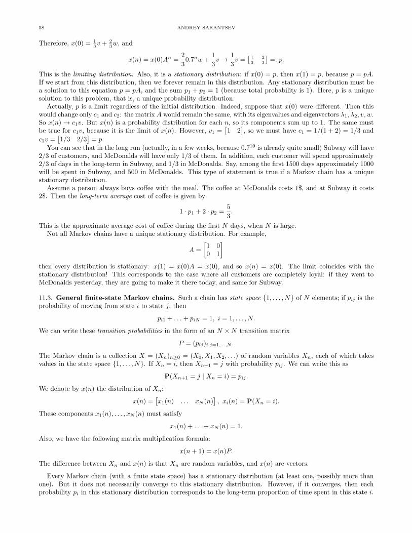
58 ANDREY SARANTSEV

Therefore, x(0) = 13v + 2

3w, and

x(n) = x(0)An =2

30.7nw +

1

3v → 1

3v =

[13

23

]=: p.

This is the limiting distribution. Also, it is a stationary distribution: if x(0) = p, then x(1) = p, because p = pA.If we start from this distribution, then we forever remain in this distribution. Any stationary distribution must bea solution to this equation p = pA, and the sum p1 + p2 = 1 (because total probability is 1). Here, p is a uniquesolution to this problem, that is, a unique probability distribution.

Actually, p is a limit regardless of the initial distribution. Indeed, suppose that x(0) were different. Then thiswould change only c1 and c2: the matrix A would remain the same, with its eigenvalues and eigenvectors λ1, λ2, v, w.So x(n)→ c1v. But x(n) is a probability distribution for each n, so its components sum up to 1. The same mustbe true for c1v, because it is the limit of x(n). However, v1 =

[1 2

], so we must have c1 = 1/(1 + 2) = 1/3 and

c1v =[1/3 2/3

]= p.

You can see that in the long run (actually, in a few weeks, because 0.710 is already quite small) Subway will have2/3 of customers, and McDonalds will have only 1/3 of them. In addition, each customer will spend approximately2/3 of days in the long-term in Subway, and 1/3 in McDonalds. Say, among the first 1500 days approximately 1000will be spent in Subway, and 500 in McDonalds. This type of statement is true if a Markov chain has a uniquestationary distribution.

Assume a person always buys coffee with the meal. The coffee at McDonalds costs 1$, and at Subway it costs2$. Then the long-term average cost of coffee is given by

1 · p1 + 2 · p2 =5

3.

This is the approximate average cost of coffee during the first N days, when N is large.Not all Markov chains have a unique stationary distribution. For example,

A =

[1 00 1

]then every distribution is stationary: x(1) = x(0)A = x(0), and so x(n) = x(0). The limit coincides with thestationary distribution! This corresponds to the case where all customers are completely loyal: if they went toMcDonalds yesterday, they are going to make it there today, and same for Subway.

11.3. General finite-state Markov chains. Such a chain has state space 1, . . . , N of N elements; if pij is theprobability of moving from state i to state j, then

pi1 + . . .+ piN = 1, i = 1, . . . , N.

We can write these transition probabilities in the form of an N ×N transition matrix

P = (pij)i,j=1,...,N .

The Markov chain is a collection X = (Xn)n≥0 = (X0, X1, X2, . . .) of random variables Xn, each of which takesvalues in the state space 1, . . . , N. If Xn = i, then Xn+1 = j with probability pij . We can write this as

P(Xn+1 = j | Xn = i) = pij .

We denote by x(n) the distribution of Xn:

x(n) =[x1(n) . . . xN (n)

], xi(n) = P(Xn = i).

These components x1(n), . . . , xN (n) must satisfy

x1(n) + . . .+ xN (n) = 1.

Also, we have the following matrix multiplication formula:

x(n+ 1) = x(n)P.

The difference between Xn and x(n) is that Xn are random variables, and x(n) are vectors.

Every Markov chain (with a finite state space) has a stationary distribution (at least one, possibly more thanone). But it does not necessarily converge to this stationary distribution. However, if it converges, then eachprobability pi in this stationary distribution corresponds to the long-term proportion of time spent in this state i.


11.4. Rate of convergence. Consider the transition matrix

A =

0 0.3 0.70.2 0.8 01 0 0

It has a unique stationary distribution p =

[p1 p2 p3

], which can be found from

p = pA, p1 + p2 + p3 = 1.

Let us solve this system of equations:

p1 = 0.2p2 + p3, p2 = 0.3p1 + 0.8p2, p3 = 0.7p1.

Therefore, from the second equation we get:

0.2p2 = 0.3p1 ⇒ p2 = 1.5p1.

And p3 = 0.7p1, so 1 = p1 + p2 + p3 = (1.5 + 1 + 0.7)p1 = 3.2p1, and p1 = 1/3.2 = 5/16, p2 = 15/32, p3 = 7/32.What is the rate of convergence of x(n) = x(0)An, the distribution at the nth step, to this distribution? Let usfind eigenvalues and eigenvectors of A. Eigenvalues:

λ1 = 1, λ2 =1

10

(√57− 1

), λ3 =

1

10

(−√

57− 1).

We have: |λ2| < |λ3| < 1. Let v1, v2, v3 be eigenvectors corresponding to λ1, λ2, λ3:

v1λ1 = v1A, v2λ2 = v2A, v3λ3 = v3A.

We can take v1 = p because λ1 = 1. Then for any initial distribution x(0) we can decompose

x(0) = c1v1 + c2v2 + c3v3,

for some numbers c1, c2, c3, and

x(n) = x(0)An = c1v1An + c2v2A

n + c3v3An = c1p+ c2λ

n2 v2 + c3λ

n3 v3.

As n→∞, x(n)→ c1p. But we know that x(n)→ p, so c1 = 1. Therefore,

x(n)− p = c2λn2 v2 + c3λ

n3 v3,

|x(n)− p| ≤ c2|λ2|n|v2|+ |c3||λ3|n|v3|.As n→∞, |λ2|n converges to zero faster than |λ3|n, because |λ2| < |λ3|. Therefore, the whole expression

c2|λ2|n|v2|+ |c3||λ3|n|v3|converges to zero with the same rate as |c3||λ3|n|v3|. We say that the rate of convergence is |λ3|n (because the restare just constants, independent of n).

11.5. Recurrence and transience. Let fi := P(S ever returns to the state i | S0 = i) be the probability thatthe Markov chain returns to the position i if it started from i. The state i is called recurrent if fi = 1, and transientfi < 1. If the state i is recurrent, then the process returns to i. But then, starting again from there, it againreturns to i, and again, etc. So the process returns to the recurrent state infinitely often. If Ni is the number oftimes when the process returns to i, then Ni =∞, and ENi =∞.

For a transient state i, with probability 1 − fi the process never returns there. With probability fi, it doesreturn there. After this, with probability fi(1 − fi), it never returns there again. With probability f2

i , it returnsthere for the second time. With probability f2

i (1− fi), it never returns there again, etc. So

P(Ni = k) = fki (1− fi), k = 0, 1, 2, . . .

Therefore, Ni has geometric distribution with parameter 1 − fi, and ENi = (1 − fi)−1 < ∞. If we start from astate and then return there infinitely many times, this state is recurrent; otherwise, it is transient.

Example 11.1. Consider the following Markov chain:

A =

0.3 0 0.70.4 0 0.60 0 1

We can draw the diagram

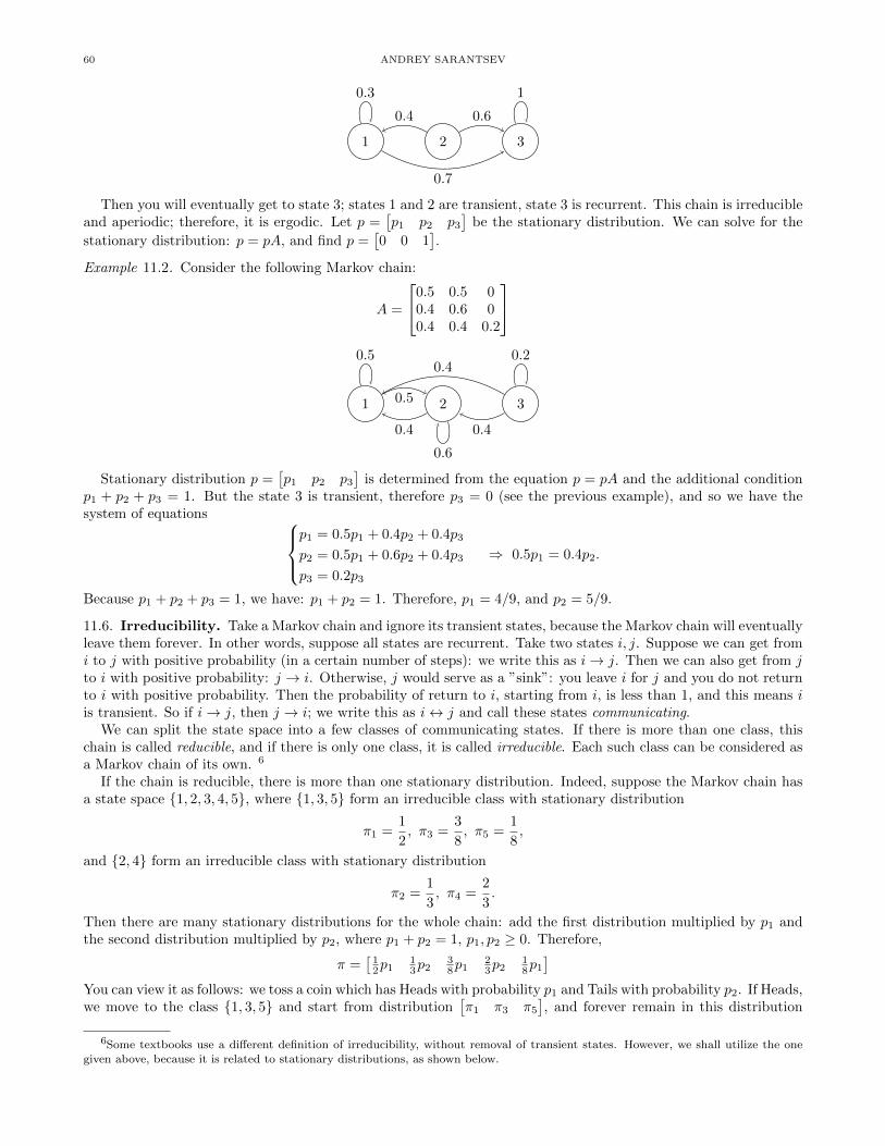
60 ANDREY SARANTSEV

1 2 3

0.3 1

0.7

0.4 0.6

Then you will eventually get to state 3; states 1 and 2 are transient, state 3 is recurrent. This chain is irreducibleand aperiodic; therefore, it is ergodic. Let p =

[p1 p2 p3

]be the stationary distribution. We can solve for the

stationary distribution: p = pA, and find p =[0 0 1

].

Example 11.2. Consider the following Markov chain:

A =

0.5 0.5 00.4 0.6 00.4 0.4 0.2

1 2 3

0.5

0.6

0.20.4

0.4

0.5

0.4

Stationary distribution p =[p1 p2 p3

]is determined from the equation p = pA and the additional condition

p1 + p2 + p3 = 1. But the state 3 is transient, therefore p3 = 0 (see the previous example), and so we have thesystem of equations

p1 = 0.5p1 + 0.4p2 + 0.4p3

p2 = 0.5p1 + 0.6p2 + 0.4p3

p3 = 0.2p3

⇒ 0.5p1 = 0.4p2.

Because p1 + p2 + p3 = 1, we have: p1 + p2 = 1. Therefore, p1 = 4/9, and p2 = 5/9.

11.6. Irreducibility. Take a Markov chain and ignore its transient states, because the Markov chain will eventuallyleave them forever. In other words, suppose all states are recurrent. Take two states i, j. Suppose we can get fromi to j with positive probability (in a certain number of steps): we write this as i→ j. Then we can also get from jto i with positive probability: j → i. Otherwise, j would serve as a ”sink”: you leave i for j and you do not returnto i with positive probability. Then the probability of return to i, starting from i, is less than 1, and this means iis transient. So if i→ j, then j → i; we write this as i↔ j and call these states communicating.

We can split the state space into a few classes of communicating states. If there is more than one class, thischain is called reducible, and if there is only one class, it is called irreducible. Each such class can be considered asa Markov chain of its own. 6

If the chain is reducible, there is more than one stationary distribution. Indeed, suppose the Markov chain hasa state space 1, 2, 3, 4, 5, where 1, 3, 5 form an irreducible class with stationary distribution

π1 =1

2, π3 =

3

8, π5 =

1

8,

and 2, 4 form an irreducible class with stationary distribution

π2 =1

3, π4 =

2

3.

Then there are many stationary distributions for the whole chain: add the first distribution multiplied by p1 andthe second distribution multiplied by p2, where p1 + p2 = 1, p1, p2 ≥ 0. Therefore,

π =[

12p1

13p2

38p1

23p2

18p1

]You can view it as follows: we toss a coin which has Heads with probability p1 and Tails with probability p2. If Heads,we move to the class 1, 3, 5 and start from distribution

[π1 π3 π5

], and forever remain in this distribution

6Some textbooks use a different definition of irreducibility, without removal of transient states. However, we shall utilize the one

given above, because it is related to stationary distributions, as shown below.


(because it is stationary). If Tails, we move to the class 2, 4 and start from the distribution[π2 π4

], and forever

remain in this distribution. For example, take p1 = 3/4 and p2 = 1/4; then

π =[

38

112

932

16

332

]We might also take p1 = 0 and p2 = 1; then we only move in the class 2, 4, and

π =[0 1

3 0 23 0

]

1 3 5 2 4

We showed that if a Markov chain is reducible, then there are multiple stationary distributions. (Because thereexists a stationary distribution for each communicating class, and we can combine them as above in many ways.)We can also show the following theorem.

If a Markov chain is irreducible, then there is only one stationary distribution.

11.7. Aperiodicity. Again, ignore transient states, and suppose the Markov chain is irreducible (or, in case it isreducible, move to any class of communicating states). Start with some element i and find the number of stepsneeded to get there; let ϕ1, ϕ2, . . . be numbers of steps for different paths. Take d, the greatest common divisor ofϕ1, ϕ2, . . .. This is called the period of this Markov chain. It does not depend on i. This means we can split thestate space into d subclasses such that if you start in the 1st subclass, at the next step you get to the 2nd one, etc.to the dth one, and then to the first one. If d = 1, the Markov chain is called aperiodic, and if d ≥ 2, it is calledperiodic. If there is a loop (there exists a state from which you can return to itself at the next step), then ϕ1 = 1,and d = 1.

As mentioned before, there exists a unique stationary distribution p. However, if d ≥ 2 (the chain is periodic),then it might not converge to this stationary distribution p. That is, not necessarily x(n)→ p as n→∞. 7

Example 11.3. Consider a Markov chain with the state space 1, 2 and the transition matrix

A =

[0 11 0

]This chain is 2-periodic, and its stationary distribution p satisfies

p = pA ⇒p1 = p2

p2 = p1

⇒ p1 = p2 =1

2.

But if x(0) =[1/3 2/3

], then x(1) = x(0)A =

[2/3 1/3

], x(2) = x(1)A =

[1/3 2/3

], etc. So

x(n) = x(0) for even n, x(n) = x(1) for odd n.

Therefore, x(n) does not have a limit. The distribution switches between x(0) and x(1).

If the Markov chain is irreducible and aperiodic, then x(n)→ p for n→∞, regardless of the initial distributionx(0). Moreover, pi > 0 for each state i. In this case, the Markov chain is called ergodic.

11.8. Summary. When we analyze a Markov chain X, the following steps are required:

Identify all transient and all recurrent states: For every state, you should find whether it is transient or recurrent.Then remove all transient states. You get a certain Markov chain Y , with all states being recurrent.

Is the resulting Markov chain Y irreducible? That is, can you get from any state to any state? If yes, the Markovchain is irreducible. If not, it splits into more than one communicating classes C1, . . . , Cr. Each such class is byitself an irreducible Markov chain, with all its states being recurrent.

Each such communicating class has a unique stationary distribution. In fact, an irreducible Markov chain hasa unique stationary distribution. If the class Ci has a stationary distribution πi, then we can weigh them (asexplained earlier in this section) with certain weight coefficients p1, . . . , pr which satisfy

p1, . . . , pr ≥ 0, p1 + . . .+ pr = 1,

7Some textbooks use another definition of aperiodicity, without removal of transient states. However, we shall remove transient

states first, because the connection to stationary distributions becomes clearer.

62 ANDREY SARANTSEV

and get a stationary distribution π for the Markov chain Y . If a Markov chain is reducible (that is, if it consists ofmore than one communicating class), then it has more than one (in fact, infinitely many) stationary distributions,because p1, . . . , pr can be chosen in multiple ways.

Every stationary distribution of Y corresponds to a stationary distribution of X: add zeroes in the places cor-responding to the removed transient states. Every stationary distribution has zeroes in components correspondingto every transient state.

The stationary distribution for an irreducible Markov chain Z = (Zn)n≥0 has the meaning of long-term timeproportions spent in this state. Take the state i, and let πi be the corresponding component of the stationarydistribution π. Let Ni(n) be the number of steps k = 1, . . . , n spent in i: Zk = i. Then we have:

Ni(n)

n→ πi a.s. as n→∞.

In particular, if i is a transient state, then the Markov chain spends only finitely many steps in i. Say it spends Mi

steps there. Then Ni(n) = Mi for large enough n, so Ni(n) does not grow as n→∞. Thus,

Ni(n)

n→ 0 a.s. as n→∞.

However, if i is a recurrent state, then πi > 0. In other words, the long-term proportion of steps spent at i ispositive. During the first n steps for a large n, the Markov chain spends approximately πin steps in the state i.

Finally, fix a communicating class; or, alternatively, assume the Markov chain is irreducible and does not containany transient states. We can find its period d by fixing the state i, and taking the gcd of lengths of all paths returningfrom i to i, as explained above. This number is the same for all states i. Fix a state i; it is in a subclass D0. Allstates j where you can go from i in one step belong to the next subclass D1. All states where you can get in onestep from some states in D1 form the subclass D2, etc. The whole Markov chain now is split into d subclassesD0, . . . , Dd−1, and the dynamics is as follows:

D0 ⇒ D1 ⇒ D2 ⇒ . . .⇒ Dd−1 ⇒ D0.

If an irreducible Markov chain is aperiodic (d = 1), then for every initial distribution x(0), we have convergence tothe stationary distribution:

x(n)→ π, n→∞.However, if this Markov chain is periodic (d ≥ 2), then for some initial distribution x(0) there is no such convergence.For example, consider the initial distribution concentrated on D0. That is, X0 ∈ D0: the initial state is among thestates from the subclass D0. Then at the next step the process goes to the subclass D1: X1 ∈ D1. Next,

X2 ∈ D2, X3 ∈ D3, . . . , Xd−1 ∈ Dd−1, Xd ∈ D0, Xd+1 ∈ D1, . . .

For each step n, only some of the components of the distribution x(n) are positive: those who correspond to therespective class. Others are zero. But for the stationary distribution π, all components are positive. So we cannothave convergence x(n)→ π as n→∞.

Every comunicating class has its own period; they might be different.

The overall scheme is as follows:

(1) For each state, find whether it is recurrent or transient. Remove all transient states.(2) Split the resulting Markov chain (with only recurrent states left) into communicating classes. If there is

only one, the chain is irreducible; otherwise, it is reducible.(3) For each communicating class, find its period and split into subclasses. If the period is 1, this class is

aperiodic; otherwise, it is periodic.

11.9. Time spent in transient states. Assume we have a Markov chain0.6 0.3 0.10 0.5 0.50 0 1

States 1 and 2 are transient. If we start from state 1, then every attempt to escape succeeds with probability 0.4and fails with probability 0.6. And once it leaves state 1, it never returns there. Therefore, time T1 spent in 1 isdistributed geometrically with parameter 0.4. In particular,

P(T1 = n) = 0.4 · 0.6n−1, n = 1, 2, . . . ; ET1 =1

0.4= 1.25.

Similarly, if we start from state 2, then time T2 spent in 2 is Geo(0.5), and ET2 = 1/0.5 = 2.


11.10. Comparison of hitting times. Consider the Markov chain with four states 1, 2, 3, 4 and transition matrix0.5 0.3 0.2 00.3 0.4 0.2 0.1∗ ∗ ∗ ∗∗ ∗ ∗ ∗

Let px be the probability that, starting from x, the process will reach 3 before it reaches 4. By definition,

p3 = 1, p4 = 0.p1 = 0.5p1 + 0.3p2 + 0.2p3;

p2 = 0.3p1 + 0.4p2 + 0.2p3 + 0.1p4

Derive the first equation: When we start from 1, we can move back to 1 with probability 0.5, and then we startfrom 1 again; or we can move to 2 with probability 0.3, then we start from 2, etc. We can rewrite these equationsas

0.5p1 = 0.3p2 + 0.2, 0.6p2 = 0.3p1 + 0.2.

It suffices to solve them and find p1 and p2.

11.11. Random walk on graphs. Consider a graph with finitely many vertices 1, 2, . . . , N . A Markov chainstarts from some vertex and chooses its neighbors with equal probability. We write i↔ j if the vertices i and j areconnected. Let deg i be the degree of the vertex i (the number of neighbors for i). Therefore, the transition matrixis given by

Aij =

(deg i)−1, i↔ j;

0, otherwise.

Let us take the stationary distribution

πi :=deg i

2M, i = 1, . . . , N.

where M is the total number of edges. Let us check that this is indeed a stationary distribution. For each vertexj, we have:

(πA)j =∑i

πiAij =∑i↔j

πiAij =∑i↔j

deg i

2M

1

deg i=

1

2M

∑i↔j

1 =deg i

2M.

For example, the following graph:

1 2

4 3

has M = 5, and stationary distribution

p1 = p3 =3

10, p2 = p4 =

2

10=

1

5.

This Markov chain (or, rather, its analogue for directed graph) is important for Google PageRank search algorithm:see section on simulation.

If the graph is connected, then the random walk on this graph is irreducible and has a unique stationarydistribution. However, if the graph is disconnected, then the random walk is reducible and has more than onestationary distribution.

11.12. Application: a Bonus-Malus system. An insurance company classifies car drivers into three tiers: Tier0 consists of the best drivers, tier 1 consists of not-so-good drivers, and tier 2 consists of bad drivers. This is thetable which shows the change between current year and next year, depending on the number of accidents this year:

Tier 0 1 2 ≥ 30 0 1 1 21 0 1 2 22 1 2 2 2

64 ANDREY SARANTSEV

Say, if a driver from the first tier had no accidents this year, this driver moves to the zeroth tier next year.Assume now that the number of accidents is always X ∼ Poi(2) for the first two tiers and Y ∼ Poi(3) for the worsttier. Then

P(X = 0) = e−2, P(X = 1) = P(X = 2) = 2e−2, P(X ≥ 3) = 1− 5e−2,

P(Y = 0) = e−3, P(Y ≥ 1) = 1− e−3.

The transition matrix is

P =

e−2 4e−2 1− 5e−2

e−2 2e−2 1− 3e−2

0 e−3 1− e−3

We can find the stationary distribution for this Markov chain:

[p0 p1 p2

]by solving the system of equations

pP = p. If rk is the premium for tier k, then the long-term average premium is p0r0 + p1r1 + p2r2.

Problems

For the next two problems, consider the Markov chain with transition matrix

A =

0.2 0.4 0 0.40.3 0 0.7 00.5 0 0.5 00 0.1 0.9 0

Problem 11.1. Which states are transient and which are recurrent? Is this Markov chain irreducible or reducible?What is its period?

Problem 11.2. Find the distribution of X2 given that X0 = 1.

For the next three problems, consider the Markov chain with transition matrix

A =

[0.1 0.91 0

]Problem 11.3. Which states are transient and which are recurrent? Is this Markov chain irreducible or reducible?What is its period?

Problem 11.4. Find its stationary distribution.

Problem 11.5. Find its rate of convergence.


A =

0.9 0.1 0 00.1 0.8 0.1 00 0.1 0.8 0.10 0 0.1 0.9

Its eigenvalues and eigenvectors are given by

λ1 = 0.659, λ2 = 0.8, λ3 = 1, λ4 = 0.941.

v1 =[−0.271 0.653 −0.653 0.271

]v2 =

[−1 1 1 −1

]v3 =

[−1 −1 −1 −1

]v4 =

[−0.653 −0.271 0.271 0.653

]Problem 11.6. Find its stationary distribution. If the payoff for the states 1 and 4 is 2.5, and for the states 2and 3 is 0, find the long-term average payoff.


For the next three problems, consider the Markov chain with transition matrix

A =

0.5 0 0.50 1 0

0.4 0 0.6



Problem 11.9. Find its stationary distributions.

Problem 11.10. Assuming that the Markov chain starts from X0 = 2, find P(X2 = 3).

For the next four problems, consider a Markov chain X = (Xn)n≥0 with state space 1, 2, 3 and transitionmatrix

A =

0.2 0.4 0.40.3 0 0.70.1 0.9 0

You can take as given the eigenvalues of this matrix:

λ1 = 1, λ2 ≈ −0.13, λ3 ≈ −0.787.

Assume the initial distribution is given by

P(X0 = 1) = 0.2, P(X0 = 2) = 0.5, P(X0 = 3) = 0.3,

Problem 11.11. Find P(X1 = 2).

Problem 11.12. Find P(X2 = 3, X3 = 2).

Problem 11.13. Find the stationary distribution π for this Markov chain. Assign to each state 1, 2, 3 the benefit0.4, 0.5, 0.1. Find the long-term average benefit.

Problem 11.14. Find the rate of convergence to this stationary distribution.

For the next three problems, consider a Markov chain X = (Xn)n≥0 with state space 1, 2, 3, 4 and transitionmatrix

A =

0.3 0 0.7 00.4 0.1 0.4 0.10.3 0 0.7 00 0.2 0.4 0.4

Problem 11.15. Find the distribution x(2) of X2, if the initial distribution is

x(0) =[0 1 0 0

]Problem 11.16. Find the stationary distribution for this Markov chain.

Problem 11.17. Find transient and recurrent states.

For the next four problems, consider the Markov chain with transition matrix

A =

0 0.5 0.5 00 0 0 10 0 0 11 0 0 0



Problem 11.20. Find the distribution of X1, X2, X3, and X4 if X0 = 1.

Problem 11.21. Same question if X0 = 2.


A =

0.3 0.4 0.30.5 0 0.50.1 0 0.9

Problem 11.22. Find the probability that, starting from 1, it hits 2 before 3.

Problem 11.23. Find the probability that, starting from 2, it hits 1 before 3.

For the next three problems, consider a Markov chain (Xn)n≥0 with three states 1, 2, 3:

P =

0.5 0.3 0.20.1 0.4 0.50 0.2 0.8

66 ANDREY SARANTSEV

Problem 11.24. Calculate the probability P(X2 = 1 | X0 = 1).

Problem 11.25. For the initial distribution x(0) = [0.6, 0.4, 0], find the distribution of X1.

Problem 11.26. Find the stationary distribution.

Problem 11.27. Consider a Markov chain with transition matrix

A =

[0.2 0.80.7 0.3

]Find its stationary distribution and rate of convergence.

Problem 11.28. Take a Markov chain on the state space 1, 2, 3 with transition matrix

A =

0.5 0 0.50 1 01 0 0

Which states are recurrent and which are transient? How many communicating classes does it have, and what isthe period for each of them?

For the next three problems, consider the Markov chain (Xn)n≥0 on the state space 1, 2 with

A =

[0.4 0.60.3 0.7

]Problem 11.29. Find P(X2 = 1), assuming that the initial distribution is given by

P(X0 = 1) = 0.4, P(X0 = 2) = 0.6.



Problem 11.32. Consider the Markov chain with transition matrix

A =

0.4 0.4 0.20.5 0 0.50.1 0.1 0.8

Find the probability that, starting from 1, it hits 2 before 3.


A =

0.1 0.3 0.60 0.4 0.60 0 1

Find the mean time spent at 2, starting from 1.

Problem 11.34. Invent a Markov chain with 7 states, 3 of which are transient, 4 are recurrent, such that theserecurrent states are split into two communicating classes, one of which has period 1, the other has period 2.


A =

0.8 0.2 00 0.5 0.50 0.7 0.3

Let T be the time (number of steps) spent at 1 if you start this Markov chain from 1. Which distribution does Thave? Find ET and VarT .


A =

0.4 0.2 0.3 0.10.2 0.5 0.3 00 0 0.5 0.50 0 1 0

Find transient and recurrent states.

In the next three problems, we take a graph. Consider the random walk on this graph. Write its transitionmatrix A and find all stationary distributions. Which states are transient and which are recurrent? Is this Markovchain irreducible or reducible? What is its period?


Problem 11.37. Take the graph with three vertices, 1, 2, and 3, such that 1 is connected with 2 and 3, but 2 and3 are not connected.

Problem 11.38. Take the graph with three vertices, 1, 2, and 3, but now each two vertices are connected (thatis, 1 is connected to 2 and to 3, and 2 is connected to 3).

Problem 11.39. Take the graph with four vertices, 1, 2, 3, 4, such that there are two edges: between 1 and 2,and between 3 and 4.

For the next two problems, assume we have a Bonus-Malus system of three tiers with the table below. Assumethe premium paid in the kth tier is 0.5k + 1 (measured in thousands of dollars).

Tier 0 1 ≥ 20 0 1 11 0 1 22 1 2 2

Problem 11.40. For every tier, the distribution of accidents is given by Z − 1, where Z ∼ Geo(0.5). Find thetransition matrix, and its stationary distribution. Find the long-term average premium.

Problem 11.41. Each person has an accident each month with probability (k + 1)/10, where k is the tier. Allmonths are independent. Find the transition matrix, and its stationary distribution. Find the long-term averagepremium.

12. Random Walk and the Binomial Model in Finance

12.1. Construction. Consider a sequence X1, X2, . . . of i.i.d. (independent identically distributed) random vari-ables with distribution P(Xi = 1) = p and P(Xi = −1) = q, p+ q = 1. Take

S0 := x, and Sn = Sn−1 +Xn, n = 1, 2, . . .

S1 = x+X1, S2 = x+X1 +X2, S3 = x+X1 +X2 +X3, . . .

Each time, the particle moves either one step to the right (with probability p) or one step to the left (with probabilityq). Each next step is independent of the past. An example of the trajectory starting from x = 0 is:

(S0 = 0, S1 = 1, S2 = 2, S3 = 1, S4 = 2, S5 = 3, . . .)

This process (S0, S1, . . .) = (Sn)n≥0 is called a random walk. When p = q = 1/2, this is called simple or symmetricrandom walk.

Example 12.1. Consider a random walk starting from S0 = −1 with p = 2/3 and q = 1/3. Find ES12 and VarS12.

EXk = 1 · p+ (−1) · q =1

3,

EX2k = 12 · p+ (−1)2 · q = 1, VarXk = EX2

k − (EXk)2 = 1−(

1

3

)2

=8

9.

ES12 = E [−1 +X1 + . . .+X12] = −1 + 12 · 1

3= 3

VarS12 = VarX1 + . . .+ VarX12 = 12 · 8

9=

32

3

x

y

68 ANDREY SARANTSEV

12.2. Transition probabilities. The transition probabilities are P(Sn = z | Sm = y). Let us give an example onhow to calculate them: take P(S10 = 4 | S5 = 3). The quantity of paths from (5, 3) to (10, 4): suppose the pathhas a steps up and b steps down. The total number of steps is a+ b = 5, and a− b = 1 (because the total ascentfrom 3 to 4 is 1). So a = (5 + 1)/2 = 3, and b = (5− 1)/2 = 2. The path made 3 steps up and 2 steps down. Thereare five possible slots for upward steps; we must choose three upward steps, the rest will be occupied by downwardsteps. The number of ways to choose this is

(53

)= (5 · 4)/2 = 10. Each such path has probability p3q2, and so the

total probability is

P(S10 = 4 | S5 = 3) = 10p3q2.

12.3. Recurrence and transience. Recall the definition of recurrent and transient states for random walk. LetNi be the number of times when the process returns to this state. If Ni =∞, and therefore ENi =∞, this state isrecurrent. If Ni is finite (Geometric distribution) and therefore ENi <∞, it is transient. Now, let us find which oftwo cases holds for the random walk. Since all states are alike, let us take the state i = 0. Let 1A be the indicatorof the event A:

1A =

1, if A happened;

0, if A did not happendthen E1A = P(A).

Because the random walk can return to zero only in an even number n = 2k of steps.

N0 =

∞∑n=1

1Sn=0, EN0 =

∞∑n=1

P(Sn = 0) =

∞∑k=1

P(S2k = 0).

Let us calculate P(S2k = 0). To get in 2k steps from 0 to 0, the process has to make k steps up and k steps down.

The number of ways to choose k steps upward is(

2kk

). Each such path has probability pkqk. Therefore,

P(S2k = 0) =

(2k

k

)pkqk.

Now, we need to find when the series∞∑k=1

(2k

k

)(pq)k

converges or diverges. By the Stirling formula, we have: k! ∼√

2πk(k/e)k. Therefore,(2k

k

)=

(2k)!

k!2∼√

2π · 2k(2k/e)2k(√2πk(k/e)k

)2 =22k

√πk.

The series∞∑k=1

22k

√πk

(pq)k =

∞∑k=1

(4pq)k√πk

converges if 4pq < 1, because of the geometric series:

∞∑k=1

(4pq)k√πk≤∞∑k=1

(4pq)k <∞.

And it diverges if 4pq = 1, because∞∑k=1

1√πk

=∞.

Now, if p = q = 1/2, then 4pq = 1, and otherwise 4pq = 4p(1− p) < 1. Indeed,

1− 4p(1− p) = 1− 4p+ 4p2 = (1− 2p)2 ≥ 0,

and this equals to zero only if p = 1/2. Result: for the symmetric random walk, every state is recurrent;otherwise, every state is transient.


12.4. Gambler’s ruin. Consider a random walk X0, X1, X2, . . ., with probability p of going up and probability qof going down. Suppose X0 = n. What is the probability qn that this random walk hits N before hitting zero?We can restate it: if a gambler wants to get N dollars, starting from n dollars, but does not want to go bankruptbefore that, what is the probability that he can pull this out?

Let us deduce this for N = 3, p = .25, q = .75. We will simulateously deduce this for n = 0, 1, 2, 3. At the firststep, starting from n, the random walk can either go up (with probability p) and reach n + 1 or go down (withprobability q) and reach n− 1. Therefore,

(17) qn = pqn+1 + qqn−1, n = 1, . . . , N − 1.

Also, q0 = 0, because if the gambler already had nothing in the beginning, he is bankrupt. And qN = 1, because ifthe gambler started with N dollars, he already achieved this goal. Plugging n = 1 and n = 2 in (17), we get:

q2 = .25 · q3 + .75 · q1 = .25 + .75 · q1; q1 = .25 · q2 + .75 · q0 = .25 · q2.

Solving this system, we get: q2 = .25 + .75 · .25 · q2 = 1/4 + (3/16)q2, therefore q2 = 4/13, and q1 = .25q2 = 1/13.In general case, we get with α = q/p:

qk =

1−αk1−αN , α 6= 1;kN , α = 1.

If p > q, then α < 1, and as N →∞, we have:

qk → 1− αk > 0.

Therefore, 1−αk is the probability of never becoming bankrupt for a good gambler: with α < 1, who is more likelyto win than lose at each step, who is playing against a bank with an infinite amount of money.

12.5. Reflection principle. Consider (Sn)n≥0, a random walk. Let us find the quantity of paths from S2 = 1 toS12 = 3 such that they do not hit or cross the line y = −1.

First, let us find the quantity of all paths from S2 = 1 to S12 = 3, that is, from (2, 1) to (12, 3), regardless ofwhether they cross or hit this line. Let n and m be the quantity of up and down steps. Then the total number ofsteps is n+m = 12− 2 = 10, and the change in altitude is n−m = 3− 1 = 2. Therefore, n = 6 and m = 4. Thereare

(106

)ways to choose 6 upward steps out of 10, so

(106

)such random walk paths.

Then, let us find the quantity of these paths that do hit or cross this line y = −1. Starting from this hittingpoint, reflect them across this line. Then we get a new random walk path, which goes from (2, 1) to (12,−5) (thepoint symmetric to (12, 3) with respect to the line y = −1). Every path from (2, 1) to (12, 3) which hits y = −1corresponds to a path from (2, 1) to (12,−5), and vice versa. Let us find the quantity of paths from (2, 1) to(12,−5). If it has n steps up and m steps down, then n+m = 12− 2 = 10 and n−m = (−5)− 1 = −6. Therefore,n = 2 and m = 8. The number of such paths is

(108

)Thus, the quantity of paths from (2, 1) to (12, 3) which do not cross the line y = −1 is

(106

)−(

108

)= 10·9·8·7

4! −(10·9

2

)= 210− 45 = 165.

x

y

y = −1

Another way to say that the path (Sn)n≥0 of random walk from (2, 1) to (12, 3) does not cross or hit y = −1 is

S12 = 3, Sn ≥ 0, n = 2, . . . , 12.

70 ANDREY SARANTSEV

Assume we have a random walk with p = 0.6 and q = 0.4. Every such path has 6 steps up and 4 steps down (seeabove), and the probability of each such path is p6q4. Therefore, the probability of this event is

P (S12 = 3, Sn ≥ 0, n = 2, . . . , 12 | S2 = 1) = 165 · p6q4

12.6. The ballot problem. Assume there were 1000 voters and two candidates, A and B, who got 600 and 400votes, respectively. Therefore A won. We start counting ballots.

How many different paths of counting ballots, that is, random walks (Sn)n≥0 from (0, 0) to (1000, 200)? Here,Sn is the ballots cast for A minus ballots cast for B when nth ballot has been counted. Therefore, S0 = 0 andS1000 = 600− 400 = 200. There has to be 600 ballots for A, and there are 1000 total ballots. The number of waysto choose them is

(1000600

).

How many such paths when A is always ahead of B? The first ballot must be for A, otherwise B immediatelycomes ahead. Next, how many paths from (1, 1) to (1000, 200) which do not hit the line y = 0? Similarly to theprevious subsection, we can find: Each such path has n steps up and m steps down, with n+m = 1000− 1 = 999,and n−m = 200− 1 = 199. Therefore, n = 599, m = 400, and there are

(999400

)such paths.

How many such paths do cross or hit this line? Reflect it, starting from the first hitting point, across this liney = 0. Then we get a random walk path from (1, 1) to (1000,−200). It has n steps up and m steps down, withn+m = 1000− 1 = 999, and n−m = −200− 1 = −201. Therefore, n = 399 and m = 600. There are

(999399

)such

paths. Therefore, the number of ways to count ballots such that A is always ahead of B is:(999

400

)−(

999

399

)We can rewrite this as (because 1000! = 1000 · 999! and 600! = 600 · 599!)

999!

599!400!− 999!

399!600!=

600

1000

1000!

600!400!− 400

1000

1000!

600!400!=

600− 400

1000

(1000

600

).

The probability that A was always ahead of B is

600− 400

1000=

1

5

12.7. The maximum of a random walk. Using the reflection principle, we can find the distribution of themaximum

Mn := max(S0, S1, . . . , Sn)

of the symmetric random walk, with p = q = 0.5. For example, let us find P(M10 ≥ 5). This event M10 ≥ 5 canhappen in two cases: (a) S10 ≥ 5; (b) M10 ≥ 5 but S10 < 5. By reflection principle, the probability of the secondevent is equal to P(S10 > 5).

x

y

y = 5

Indeed, starting from the first hitting point of the line y = 5, we reflect this trajectory of a random walk acrossthis line. Thus,

(18) P(M10 ≥ 5) = P(S10 ≥ 5) + P(S10 > 5) = P(S10 ≥ 5) + P(S10 ≥ 6).


Similarly, substituting 6 instead of 5 and 7 instead of 6, we get:

(19) P(M10 ≥ 6) = P(S10 ≥ 6) + P(S10 ≥ 7).

Subtract (19) from (18) and get:

(20) P(M10 = 5) = P(S10 = 5) + P(S10 = 6).

But S10 can take only even values, therefore the first term in the right-hand side of (20) is zero, and (20) takes theform

P(M10 = 5) = P(S10 = 6).

This we can find, as explained earlier: If the path with S10 = 6 takes a steps up and b steps down, then a+ b = 10and a− b = 6, so a = 8 and b = 2. Each given path has probability 2−10. Thus

P(S10 = 6) = 2−10

(10

2

)=

10 · 92 · 1024

= 0.0439.

12.8. Financial modeling. Random walk is used for elementary modeling of movements of the stock. Assume Pnis the price of a stock at day n. We can model it as a geometric random walk: Pn = P0Z1 . . . Zn, where Z1, . . . , Znare i.i.d. positive random variables. Take a random walk S = (Sn)n≥0 starting from S0 = x, with probabilities pand q of moving up and down. Then we let

Pn = exp (σSn + bn) , n = 0, 1, 2, . . .

for some coefficients σ > 0 and b. The coefficient σ is called volatility, since it is responsible for random fluctuations.The coefficient b is called drift. We can alternatively write this as follows:

Pn = exp

(σ

n∑k=1

Xk + bn

)= exp

(n∑k=1

Yk

),

where Yk = σXk + b. All Y1, Y2, . . . are i.i.d. and have distribution

P(Yk = b+ σ) = p, P(Yk = b− σ) = q.

Example 12.2. For p = q = 0.5 (symmetric random walk), drift b = −2 and volatility σ = 3, find EP10 if P0 = 2.We have:

EeYk = 0.5e−2+3 + 0.5e−2−3 = 0.5(e+ e−5

)= 1.363.

Therefore,EP10 = E

[P0e

Y1eY2 . . . eY10]

= 2E[eY1]· . . . ·E

[eY10

]= 2 · 1.36310 = 44.1.

Example 12.3. For p = 0.75, q = 0.25, b = 1 and σ = 2, given that P0 = 0.5, what are the possible values of P3,and what is the distribution of P3? Each random variable Yk takes values 3 and −1 with probabilities p and q,respectively. Therefore, the possible values of P3 are

P3 = e3+3+3P0 =e9

2, with probability p3;

P3 = e3+3−1P0 =e5

2, with probability 3p2q;

P3 = e3−1−1P0 =e

2, with probability 3pq2;

P3 = e−1−1−1P0 =e−3

2, with probability q3.

12.9. Options and other derivatives. Assume the price of a stock is modeled by (Pn)n≥0, as above. A Europeanoption call is the right to buy this stock at a given price K, called the strike, at some future time T , called thematurity. A European option put is the right to sell this stock at the price K at time T . Let us find the values ofthese options.

If the stock price PT at maturity is less than K, then it makes no sense to exercise the European option call:We can just buy the stock on the free market. Therefore, the price of the option is zero. However, the Europeanoption put is valuable, and its value is K − PT . For the case PT > K, the situation is reversed: The value of theEuropean option call is PT − K, and the European option put has value 0. Thus, if we denote a+ := max(a, 0)for every real number a, then the value of the European option call is (PT −K)+, and the value of the Europeanoption put is (K − PT )+.

An American option call/put can be exercised at any time until maturity. Therefore, such option is generallymore valuable than the corresponding European option. We shall discuss valuation of the American options later.

72 ANDREY SARANTSEV

European options are particular cases of European derivatives, which are worth f(PT ), where f(x) is a certainfunction, and T is the maturity. For example, f(x) = 1(x ≥ a) is the binary option: pay 1 if the price at maturityPT exceeded a, and pay nothing otherwise. A forward contract corresponds to f(x) = x−K, which is the obligationto buy the stock at time T for the price K. Such contracts are used by farmers and ranchers, who want to lock ingood prices (to protect themselves from downside risk), and international companies (airlines, oil, steel), who wantto lock in a certain exchange rate (say, be able to buy a euro next year using the current exchange rate, ratherthan the future exchange rate).

12.10. Hedging a derivative. This means buying a certain amount of this stock to be able to replicate thisderivative: exactly match the value of this derivative at maturity. Let us illustrate this using a one-step model:T = 1, and

P0 = 1, P1 =

1.2 with probability p = 40%;

0.6 with probability q = 60%.

We sell a European option call with maturity T = 1 and strike K = 0.9. Assume v is its current fair value. Thenwe need to use this money v to buy s stocks and c cash, and hedge the option. At time t = 0, the stock price is 1;therefore,

(21) v = s+ c.

Next, at time t = 1, if the stock price is 1.2, then we need that our portfolio (consisting of cash c and s shares) hasvalue 1.2s+ c, equal to our obligation (which is the option value):

(22) 1.2s+ c = (1.2− 0.9)+ = 0.3.

Similarly, if the stock price is 0.6, then we need:

(23) 0.6s+ c = (0.6− 0.9)+ = 0.

Solve these two equations: s = 0.5, c = −0.3. Thus, we need to borrow 0.3 in cash and buy 0.6 shares of stock.The fair value is v = −0.3 + 0.5 = 0.2. Note that this is not an expected value E(P1 − K)+, which is equal to0.3 ·40%+0 ·60% = 0.12. Rather, this is an expected value E0(P1−K)+ with respect to the risk-neutral probabilityp0, q0, such that E0P1 = P0. Let us find them:

p0 · 1.2 + q0 · 0.6 = 1

p0 + q0 = 1⇒ p0 =

2

3, q0 =

1

3⇒ E0(P1 −K)+ =

2

3· 0.3 +

1

3· 0 = 0.2.

Indeed, if we wish to get (21) as follows: multiply (22) by p0 and (23) by q0, and sum them; then to makethe coefficient at s be equal to 1, we get: p0 · 1.2 + q0 · 0.6 = 1, which is the same as E0P1 = P0. Thenv = p0 ·0.3+q0 ·0 = E0(P1−K)+. The same can be done with any other derivative with maturity T = 1. Actually,the same result is true for any maturity.

This works if P1 has only two values. If it has three or more values, or has continuous distribution (such asnormal), then the system of equations in place of (22) and (23) has three or more equations, but two variables,and it does not have a solution. Therefore, not all derivatives can be replicated. Such market is called incomplete.There is more than one risk-neutral probabilities, because there are two equations for them, but more than twovariables.

For more than one step: T ≥ 2, we hedge for every step, starting from the end: Assume Pn = P0Z1 . . . Zn, whereZi are i.i.d. with values 2 and 0.5 with some (irrelevant) probabilities. Let P0 = 1. Consider the European optioncall with maturity T = 2 and strike K = .5. We have three cases:

Z1 = Z2 = 2 : then P2 = 4, (P2 −K)+ = 3.5;

Z1 = 2, Z2 = 0.5 or Z1 = 0.5, Z2 = 2 : then P2 = 1, (P2 −K)+ = 0.5;

Z1 = Z2 = 0.5 : P2 = 0.25, then (P2 −K)+ = 0.

Assume we are at P1 = 0.5, then hedge:

c+ 0.5s = v, c+ s = 0.5, c+ 0.25s = 0 ⇒ v =0.5

3.

The risk-neutral probability in this case is 1/3 and 2/3 corresponding to the jumps up and down, because

0.5 =1

3· 1 +

2

3· 0.25.


Similarly, if P1 = 2, then

c+ 2s = v, c+ s = 0.5, c+ 4s = 3.5 ⇒ v =1

3· 3.5 +

2

3· 0.5 = 1.5.

We have fair values corresponding to P1 = 0.5 (V1 = 1/6) and P2 = 2 (V2 = 1.5), then we can hedge on the firststep, with P0 = 1:

c+ s = v, c+ 0.5s =1

6, c+ 2s = 1.5.

At every step, we take the expectation with respect to risk-neutral probability, when EZ1 = EZ2 = 1, and thereforeE(P2 | P1) = E(P1Z2 | P1) = P1EZ2 = P1, and E(P1 | P0) = EP1 = EZ1 = 1. We say that under this measure,the process (Pn)n≥0 is a martingale (see Section 13).

There is a general result (see more details in courses on stochastic finance): If there exists a unique risk-neutralprobability, then the market is complete: Every European derivative is replicable, and its fair price is the expectationwith respect to this risk-neutral probability.

Problems

For the next two problems, assume Peter and Alys are tossing a coin. Heads means Peter gets 1$ from Alys,Tails means the opposite. Initially, Peter has 7$, and Alys has 9$.

Problem 12.1. What is the probability that Peter becomes bankrupt if the coin is fair?

Problem 12.2. Same question for a biased coin, with probabilities p = 0.3 and q = 0.7 of Heads and Tailsrespectively.

Problem 12.3. Take a random walk S = (Sn)n≥0 with probability p = 1/3 of going up, starting from S0 = 1.Find the probability that this random walk hits 10 before −10.

For the next three problems, consider a random walk (Sn)n≥0 with probability p = 0.6 going upward andprobability q = 0.4 going downward.

Problem 12.4. Find the probability that P(S14 = 4 | S2 = 2).

Problem 12.5. Assume the random walk starts at S0 = 0. Find ES3 and VarS3.

Problem 12.6. Find E(S6 − S2) and Var(S6 − S2).

For the next two problems, consider a symmetric random walk (Sn)n≥0, starting from S0 = 1.

Problem 12.7. Find the probability that S10 = 1.

Problem 12.8. Find ESn and VarSn.

For the next three problems, consider a simple random walk (Sn)n≥0 starting from S0 = 0, with Mn =max(S0, S1, . . . , Sn).

Problem 12.9. Find P(M9 = 7).

Problem 12.10. Find P(M20 = 5).

Problem 12.11. Find P(M10 = 6, S10 ≥ 4). Hint: Decompose into P(M10 = 6 4 ≤ S10 ≤ 5) − P(S10 ≥ 6) andapply reflection principle to the first term.

For the next two problems, consider a random walk (Sn)n≥0 with probability p = 0.7 going upward and proba-bility q = 0.3 going downward.

Problem 12.12. Find the probability that, starting from S2 = 2, the trajectory ends at S13 = 3.

Problem 12.13. Same question, under additional condition that the trajectory does not touch y = 1.

Problem 12.14. Consider a symmetric random walk (Sn)n≥0 starting from S0 = 0. What is the probability

P(S10 = 2, Sn > −2, n = 0, . . . , 10).

For the next two problems, assume the following setting. There are two candidates, A and B, and 500 votes. Agets 350 and B gets 150. Assume the ballots are counted one by one.

Problem 12.15. Find the total quantity of ways to count the ballots.

Problem 12.16. Find the probability that A was always ahead of B during the vote counting.

74 ANDREY SARANTSEV

For the next two problems, consider a random walk (Sn)n≥0, starting from S0 = 2, with probabilties p = 0.7and q = 0.3 of up and down jumps.

Problem 12.17. Find P(S15 = 3).

Problem 12.18. Find E(S14 − S1) and Var(S14 − S1).

Problem 12.19. Take a random walk with p = 0.3 and q = 0.7. Find the probability that the random walk,starting from S0 = 3, comes to S11 = 4 without crossing or hitting the line y = 5.

For the next three problems, consider the stock market model with

p = 0.6, q = 0.4, b = 1.5, σ = 0.5, P0 = 2.

Problem 12.20. Find the distribution of P1 and of P2.

Problem 12.21. Find EP10 and VarP10.

Problem 12.22. Find P(P10 = 2e15).

For the next three problems, consider a European option put with maturity T and strike K = 1.6, on the marketmodeled as geometric random walk, with dynamics P0 = 1.5, Zk = 2 or 0.4 with equal probabilities.

Problem 12.23. Find its fair price and the replicating strategy for T = 1.

Problem 12.24. Find its fair price and the replicating strategy for T = 2.

Problem 12.25. Find its fair price for T = 3 via the risk-neutral probability.

For the next two problems, consider the same market model as for the previous three problems.

Problem 12.26. Hedge a binary option with strike K = 1.6 and maturity T = 2 from the same market as above.

Problem 12.27. Find the fair price for a European option call with T = 3, P0 = K = 1, P1 = 2 or 0.3.

13. Discrete-Time Martingales and American Derivatives

13.1. Definitions. A process X = (Xn)n≥0 is called a martingale if for each n = 0, 1, 2, . . ., we have:

(24) E(Xn+1 | X0, . . . , Xn) = Xn.

That is, if the best prediction of the next value, given all history, is the current value. If we have

(25) E(Xn+1 | X0, . . . , Xn) ≥ Xn,

then the process is called a submartingale. If we have:

E(Xn+1 | X0, . . . , Xn) ≤ Xn,

then the process is called a supermartingale.

Example 13.1. Take independent random variables Z1, Z2, . . .. Let

X0 := 0, and Xn := Z1 + . . .+ Zn for n = 1, 2, . . .

Then Xn+1 = Xn + Zn+1. Therefore,

E(Xn+1 | X0, . . . , Xn) = E(Xn | X0, . . . , Xn) + E(Zn+1 | X0, . . . , Xn) = Xn + EZn+1.

because Zn+1 is independent of X0, . . . , Xn. Thus, (Xn)n≥0 is a martingale if and only if all EZ1 = EZ2 = . . . = 0.It is a submartingale if all EZk ≥ 0, and a supermartingale if all EZk ≤ 0.

Example 13.2. Again, take independent random variables Z1, Z2, . . .. Let Yn := eXn . Then Yn+1 = YneZn+1 .

Therefore,

E(Yn+1 | Y0, . . . , Yn) = E(YneZn+1 | Y0, . . . , Yn) = YnE(eZn+1 | Y0, . . . , Yn) = YnE

[eZn+1

],

because Zn+1 is independent of Y0, . . . , Yn. Thus, (Xn)n≥0 is a martingale if and only if all EeZ1 = EeZ2 = . . . = 1.It is a submartingale if all EeZk ≥ 1, and a supermartingale if all EeZk ≤ 1.

For a submartingale X = (Xn)n≥0, taking expectations in (25), we get: E(Xn+1) ≥ EXn. Therefore,

EX0 ≤ EX1 ≤ EX2 ≤ . . .For a martingale, we have the equality. Our goal now is to show this is true for random times τ instead of fixedtimes n.


13.2. Stopping times. A random variable τ which takes values 0, 1, 2, . . . is called a stopping time if the eventτ = n depends only on X0, . . . , Xn. If Xn is the price of your stock on day n, then τ can be the moment whenyou decide to sell your stock. But you can decide whether to do this right now (on day n) or not based only onthe current information, that is, on X0, . . . , Xn; not on Xn+1, for example.

Example 13.3. The moment τ := minn : Xn > 1 is a stopping time, because τ = n means that X0 ≤ 1, X1 ≤1, . . . , Xn−1 ≤ 1, Xn > 1. So τ = n depends only on X0, . . . , Xn.

Example 13.4. Similarly, τ = minn : a ≤ Xn ≤ b is a stopping time, for fixed a and b. More generally, for everysubset D ⊆ R, τ = minn : Xn ∈ D is a stopping time.

Example 13.5. However, τ = maxn : Xn > 1 is not a stopping time. Indeed, consider the event τ = 1. Thismeans that X2 ≤ 1, so it depends on the future values of X.

13.3. Optional stopping theorem. Consider a stopping time τ whch is bounded from above by some constantN : τ ≤ N . If X = (Xn)n≥0 is a martingale, then

(26) EXτ = EXN = EX0.

Indeed, τ can take values 0, 1, . . . , N − 1, N . Therefore,

(27) EXN =

N∑n=0

E[XN1τ=n

], and EXτ =

N∑n=0

E[Xτ1τ=n

].

But τ = n depends only on X0, . . . , Xn, and E [XN | X0, . . . , Xn] = Xn. Therefore

(28) E[XN1τ=n

]= E

[E[XN1τ=n | X0, . . . , Xn

]]= E

[1τ=nE [XN | X0, . . . , Xn]

]= E

[1τ=nXn

].

Summing (28) over n = 0, . . . , N , and using (27), we complete the proof of (26).For a submartingale, we have EX0 ≤ EXτ ≤ EXN , and for a supermartingale, these inequalities are reversed.

Assume X is the price of a stock. If it is a martingale, then the optional stopping theorem means the following:Suppose you need to sell the stock by day N . Then you cannot devise a strategy (a rule) which will make youmore (expected) profit than if you simply sell the stock at the initial day. No matter how you observe and analyzethe behavior of this stock, you will not gain extra profit. However, if the price is a submartingale, then you shouldhold it and sell it at the last day. If the price is a supermartingale, you should sell it immediately.

The condition that τ is bounded is important. Consider the symmetric random walk from Section 12:

Xn = Z1 + . . .+ Zn, P(Zn = ±1) =1

2.

Since EZn = 1 · 12 + (−1) · 1

2 = 0, the process X = (Xn)n≥0 is a martingale. Let τ = minn : Xn = 1. As notedin Section 12, this stopping time is well defined, since this random walk will eventually hit level 1. But this hittingcan happen very late; this stopping time τ is unbounded. By construction, Xτ = 1, so EXτ = 1 6= 0 = EX0. Ifyou are an investor trying to sell the stock with price Xn (forgetting for a minute about the fact that stock pricescannot go negative), then your strategy τ is to sell the stock when it hits level 1. But until then, your investmentmight go far into the negative terrirory. You will need to borrow potentially unlimited amount of money, and nolender will agree to do this.

13.4. Jensen’s inequality. Recall that g : R→ R is a convex function if

g(λx+ (1− λ)y) ≤ λg(x) + (1− λ)g(y).

For example, g(x) = x and g(x) = x2 are convex functions, while g(x) = sinx is not. Equivalently, if you connectany two points on the graph of g by a segment, then it lies above the graph. For a twice differentiable function g,it is convex if and only if its second derivative is nonnegative: g′′(x) ≥ 0 for all x. Jensen’s inequality says that ifg is a convex function, then

(29) Eg(Z) ≥ g(EZ).

Indeed, let m = EZ. Since g is convex, there exists a real-valued a such that for all real x we have: g(x) −g(m) ≥ a(x − m). (The graph of g lies above the tangent line at point x = m.) Plugging in x = Z, we have:g(Z)− g(m) ≥ a(Z −m). Take the expectations:

Eg(Z)− g(m) ≥ aE(Z −m) = 0.

Therefore,

Eg(Z) ≥ g(m) = g(EZ).

76 ANDREY SARANTSEV

One example of this is a well-known fact that EZ2 ≥ (EZ)2. This is true, and EZ2 − (EZ)2 = VarZ ≥ 0. Thisimmediately follows from (29): jsut apply g(x) = x2.

Similarly, we can show (29) for conditional expectation instead of the unconditional:

(30) E [g(Z) | Y1, . . . , Yn] ≥ g (E [Z | Y1, . . . , Yn]) .

13.5. Preservation of the martingale property. Take a martingale X = (Xn)n≥0. Apply a convex function gto (24). By Jensen’s inequality (30), we have:

E [g(Xn+1) | X0, . . . , Xn] ≥ g (E [Xn+1 | X0, . . . , Xn]) = g(Xn).

Therefore, g(X) = (g(Xn))n≥0 is a submartingale.

Let us apply this to option pricing. We already discussed European options and other European derivatives inSection 12. Recall that a call option is the right to buy a stock at a certain strike price K. A European call optionhas maturity time N , when you can exercise this option: demand to buy this stock at price K. If the marketprice SN of this stock at time N is less than K, then you can just buy the stock at the market price and forgetabout your option. Then your option does not have value. However, if the market price SN ≥ K, then you shouldexercise this option, and its value is SN −K. In general, the value of this option is max(SN −K, 0) = g(SN ), whereg(x) = max(x−K, 0).

An American call option is different from a European one in the following way: the former can be exercised atany time until maturity N , while the latter must be exercised at maturity. Therefore, let τ be the time you decideto exercise your American call option to get the best expected value Eg (Sτ ). When is the best exercise time τ?This is a stopping time, since your decision to exercise at time n or not is based only on your observations untiltime n, but not on future observations. But the function g is convex (draw a graph and check). Frequently, thestock price X is modeled by a martingale. Then g(S) = (g(Sn))n≥0 is a submartingale. By the optional stoppingtheorem,

Eg (Sτ ) ≤ Eg (SN ) .

Therefore, the best time to exercise your American call option is at maturity n = N . In fact, American andEuropean call options are of the same value in this case. Additional freedom to choose exercise time does not giveyou anything.

13.6. Doob’s inequalities. These are generalizations of Markov’s and Chebyshev’s inequalities. Take a nonneg-ative submartingale X = (Xn)n≥0 and a number λ > 0. Then

P

(max

k=0,...,nXk ≥ λ

)≤ EXn

λ.

Indeed, take the stopping time τ := mink = 0, . . . , n : Xk ≥ λ, with τ = n if X0 < λ, . . . ,Xn < λ. If the event

A =

max

k=0,...,nXk ≥ λ

has happened, then Xτ ≥ λ, and

λP(A) ≤ E (Xτ1A) .

But X is nonnegative, so

E (Xτ1A) ≤ EXτ1A + EXτ1Ac = EXτ .

Because of the optional stopping theorem, EXτ ≤ EXn. Comparing this, we get:

λP(A) ≤ E (Xτ1A) ≤ EXτ ≤ EXn.

It suffices to divide by λ. A corollary: for a nonnegative submartingale or a martingale X = (Xn)n≥0, if p ≥ 1,then

P

(max

k=0,...,nXk ≥ λ

)≤ E|Xn|p

λp.

Indeed, the function x 7→ |x|p is convex for p ≥ 1, and for x ≥ 0 it is equal to xp, so it is nondecreasing.

Letting p = 2 and recalling the very first example of a martingale: Xn = Z1+. . .+Zn for independent Z1, . . . , Zn,we have the following Kolmogorov’s inequality:

P (max (X0, . . . , Xn) ≥ λ) ≤ 1

λ2EX2

n =1

λ2

N∑k=1

EZ2k .


Example 13.6. Simple random walk Sn starting from S0 = 0 is a martingale. Estimate by Kolmogorov’s inequality:

(31) P

[max

0≤n≤10|Sn| ≥ 5

]≤ ES2

10

52.

Since ES10 = 0, ES210 = VarS10 = Var(X1 + . . .+X10) = VarX1 + . . .+VarX10 = 1+ . . .+1 = 10, where Xi = ±1

with equal probabilities and are independent. Thus the right-hand side in (31) is 10/25 = 0.4

Example 13.7. Now, consider Mn = eSn−cn. Need to find n such that this is a martingale:

EeX1−c = 1 ⇒ 1

2

(e1 + e−1

)= ec ⇒ c = ln

(e1 + e−1

)− ln 2.

Apply Doob’s martingale inequality with f(x) = x3. For x > 0, this function is convex, since f ′′(x) = 6x > 0; andonly this matters, because Mn > 0 always. Thus for λ > 0 we have:

(32) P

[max

0≤n≤100Mn ≥ λ

]≤ E

[M3

100

]λ3

.

Now we calculate the right-hand side of (32):

(33) M3100 = e3S100e−300c = e3X1e3X2 . . . e3X100e−300c.

All terms in the right-hand side of (33) are independent, so we can calculate the expectation:

E[M100

3

]= e−300c

(E[e3X1

])100= e−300c

(1

2

[e3 + e−3

])100

.

Problems

For the next three problems, find the values of parameters for which the process S = (Sn)n≥0, defined as

Sn := X1 + . . .+Xn for n = 1, 2, . . . , and S0 := 0,

is a martingale, submartingale, supermartingale.

Problem 13.1. Let X1, X2, . . ., the i.i.d. Bernoulli with P(Xi = 1) = p and P(Xi = 0) = q.

Problem 13.2. Let X1, X2, . . . ∼ N (µ, σ2) be i.i.d. normal.

Problem 13.3. Let Xn = Zn − 2, where Zn ∼ Exp(λ) are i.i.d.

For the next three problems, find the values of parameters for which the process M = (Mn)n≥0, defined as

Mn := e2Sn−3n, n = 0, 1, 2, . . .

is a martingale, submartingale, supermartingale.

Problem 13.4. Same as Problem 13.1.



For the next seven problems, take a process X = (Xn)n≥0 and find whether τ is a stopping time.

Problem 13.7. τ := minn | Xn ≥ 2.Problem 13.8. τ := minn | X2

n − 3Xn + 1 = 0.Problem 13.9. τ : minn | Xn+1 ≥ 0.Problem 13.10. τ := minn | Xn−1 ≥ 0.Problem 13.11. τ := maxn | Xn−1 = 1.Problem 13.12. τ := minn | Xn +Xn+1 = 0.Problem 13.13. τ := minn | Xn = Xn−1.Problem 13.14. τ := min(minn | Xn = 3, 4).

Problem 13.15. τ := 4−min(minn | Xn = 3, 4).

For the next four problems, find whether the following functions are convex.

Problem 13.16. g(x) = x4 + x2.

78 ANDREY SARANTSEV

Problem 13.17. g(x) = x4 − x2.

Problem 13.18. g(x) = cosx.

Problem 13.19. g(x) = e2x+1.

For the next two problems, consider the following setting. Toss a fair coin repeatedly. Let Xn be the number ofHeads during the first n tosses for n = 1, 2, . . ., and let X0 := 0.

Problem 13.20. Find a constant c such that the process (Yn)n≥0 is a martingale: Yn := 3Xn − cn.

Problem 13.21. Find c such that M = (Mn)n≥0 is a martingale: Mn := e2Xn+cn.

For the next five problems, consider a derivative f(Pt) of the stock with price Pt at time t, which forms amartingale. Is it optimal to exercise the American version at maturity time?

Problem 13.22. f(x) = x2 + x.

Problem 13.23. A put option.

Problem 13.24. A binary option.

Problem 13.25. f(x) = 4x3.

Problem 13.26. f(x) = (x− 1)3.

For the next three problems, apply Kolmogorov’s inequality to the martingale (Mn)n≥0 to estimate from above:

(34) P (max(|M0|, . . . , |M100|) ≥ λ) .

Problem 13.27. Mn = 2 +X1 + . . .+Xn, Xi ∼ N (0, 2) i.i.d.

Problem 13.28. Mn = eSn−cn, Sn = −1 + X1 + . . . + Xn, Xi ∼ N (0, 4) i.i.d. and find the c such that this is amartingale.

Problem 13.29. Mn = c−nZ1 · . . . · Zn, Zi ∼ Exp(2) i.i.d. and find the c such that this is a martingale.

For the next two problems, apply Doob’s martingale inequality with a given convex function f(x) to estimate (34):

Problem 13.30. Mn = eSn−cn, Sn = −1 +X1 + . . .+Xn, Xi ∼ N (0, 4) i.i.d., f(x) = x3.

Problem 13.31. Mn = c−nZ1 · . . . · Zn, Zi ∼ Exp(2) i.i.d., f(x) = x4.

14. Poisson Process and Compound Poisson Process

14.1. Poisson process. Fix a positive real number λ. A collection N = (N(t), t ≥ 0), of random variables withvalues in Z+ := 0, 1, 2, . . . is called a Poisson process if: N(0) = 0, and for every 0 ≤ s < t, N(t) − N(s) isdistributed as a Poisson random variable Poi(λ(t− s)) and is independent of N(u), u ≤ s. In particular,

N(t) ∼ Poi(λt); P(N(t) = k) =(λt)k

k!e−λt, k = 0, 1, 2, . . .

This process is used, among other applications, to model arrival of insurance claims, and a stock price. Since aPoisson random variable with parameter µ has mean and variance µ, we have: EN(t) = VarN(t) = λt.

Example 14.1. Take λ = 3. What is the probability that N(5) = 3, given N(2) = 1, for the same Poisson process?

P(N(5) = 3 | N(2) = 1) = P(N(5)−N(2) = 2 | N(2) = 1) = P(N(5)−N(2) = 2)

= P(Poi(3 · 3) = 2) =92

2!e−9 =

81

2e−9.

P(N(5) = 3, N(2) = 1) = P(N(5) = 3 | N(2) = 1) ·P(N(2) = 1) =81

2e−9 · 61

1!e−6 = 243e−15

Example 14.2. Take λ = 3. Then N(2) ∼ Poi(6), therefore EN(2) = 6 and VarN(2) = 6. Thus

EN2(2) = VarN(2) + (EN(2))2 = 6 + 62 = 42

Also, by independence of N(2) and N(5)−N(2), we have:

E [N(2)N(5)] = EN2(2) + E [N(2)(N(5)−N(2))] = 42 + EN(2) ·E [N(5)−N(2)] = 42 + 2λ · (5− 2)λ = 96


x

y

x

y

Left picture: Poisson process with intensity λ = .5. Right picture: Compound Poisson process with the samePoisson process (and the same trajectory) as on the left picture, and with increments distributed as N (0, 1)

14.2. Jump times of Poisson process. Note that Poisson random variable is nonnegative, and so for s ≤ t, wehave: N(t) − N(s) ≥ 0. Therefore, the process N is nondecreasing: N(t) ≥ N(s). It starts from 0, then jumpsto 1 after waiting an exponential time τ1 ∼ Exp(λ). Why? Because the probability that this process has notyet jumped by time t is equal to the probability that N(t) = 0. Letting k = 0 into the formula above, we get:P(N(t) = 0) = e−λt. Therefore,

P(τ1 > t) = e−λt.

This means that τ1 ∼ Exp(λ). This random variable has cumulative distribution function and density

F (t) = P(τ1 ≤ t) = 1− e−λt, p(t) = F ′(t) = λe−λt, t > 0.

This random variable has Eτ1 = λ−1 and Var τ1 = λ−2.After jumping to τ1, the process waits some random time and jumps from 1 to 2. If τ2 is the time when it jumps

from 1 to 2, then τ2 − τ1 is the time which it waits between its first and second jumps. It turns out that τ2 − τ1 isindependent from τ1 and is also distributed as Exp(λ). The reason for this is when the process N jumps to 1, it“forgets the past” and behaves as if instead of 1 it was at 0 and nothing yet has happened. This follows from theproperty above: that N(t) − N(s) for t > s is independent of N(u) for u ≤ s. This important property is calledthe Markov property, after a Russian mathematician Andrey Markov.

Similarly, if τk is the time of jump from k − 1 to k, then τk − τk−1, τk−1 − τk−2, . . . , τ2 − τ1, τ1 are i.i.d. Exp(λ)random variables. It is possible to show that this process does not jump, say, from 0 to 2: all its jumps havemagnitude 1.

Let us now find the distribution of τ2. This is a sum of two independent random variables τ1 and τ2 − τ1, bothwith density p1(t) = λe−λt for t > 0. As mentioned in subsection 5.8, the density p2(x) of τ2 is then the convolutionof these exponential densities:

p2(x) =

∫ x

0

p1(y)p1(x− y) dy = λ2xe−λx.

It was calculated in subsection 5.9. More generally, the density pk of τk is given by

pk(x) =λk

(k − 1)!xk−1e−λx, x > 0.

This is called the Gamma distribution Γ(k, λ) with parameters k and λ. It has expectation and variance (becauseof independence):

Eτk = Eτ1 + E(τ2 − τ1) + . . .+ E(τk − τk−1) = kλ−1,

Var τk = Var τ1 + Var(τ2 − τ1) + . . .+ Var(τk − τk−1) = kλ−2.

Example 14.3. What is the probability that the Poisson process with λ = 3, by time t = 4, has jumped two ormore times?

P(τ2 ≤ 4) = P(N(4) ≥ 2) = 1−P(N(4) = 0)−P(N(4) = 1).

Since N(4) ∼ Poi(12), this becomes

1− 120

0!e−12 − 121

1!e−12 = 1− 13e−12

80 ANDREY SARANTSEV

14.3. Compound Poisson process. Now, we modify the Poisson process to let it jump not only by 1 upward, butin a more general way. Define a sequence of i.i.d. (independent identically distributed) random variables Z1, Z2, . . .,independent of N(t), t ≥ 0). Then a compound Poisson process is defined as

X(t) =

N(t)∑k=1

Zk.

It starts from X(0) = 0, then waits time τ1 and jumps to X(τ1) = Z1. Next, it waits time τ2 − τ1 and jumps toX(τ2) = Z1 + Z2, then waits time τ3 − τ2 and jumps to X(τ3) = Z1 + Z2 + Z3, etc.

This process also has the property that X(t) − X(s) is independent of X(u), u ≤ s (Markov property), butit is distributed usually not as a Poisson random variable. The distribution of X(t) − X(s) is the same as thedistribution of X(t − s), because they are sums of N(t) −N(s) and, respectively, N(t − s)i.i.d. random variablesZ1, Z2, . . . but N(t)−N(s) and N(t− s) have the same distribution.

To find the distribution of X(t), let us recall the theory of Section 8: random sum of random numbers. Thegenerating function ϕN(t)(s) of N(t) ∼ Poi(λt) is given by

ϕN(t)(s) = EsN(t) = eλt(s−1).

Assume FZ(y) = EeyZi is the moment generating function of each Zi; it is independent of i, since Z1, Z2, . . . havethe same distribution. Then by results of Section 8 (random sum of random variables), we have: the momentgenerating function of X(t) is equal to

Gt(y) := EeyX(t) = ϕN(t)(FZ(y)) = exp (λt(FZ(y)− 1)) .

We can also find expectation and variance, using the formulas from Section 8. Assume EZk = µ, and VarZk = σ2.Because EN(t) = VarN(t) = λt,

(35) EX(t) = EN(t) ·EZk = λµt,

(36) VarX(t) = EN(t) ·VarZk + VarN(t) · (EZk)2 = λ(σ2 + µ2)t.

14.4. Sampling from a Poisson process. One can consider the Poisson process N = (N(t), t ≥ 0) with intensityλ, as the process of arrival of customers with interarrival times independent Exp(λ). Now assume that ”good”customers arrive with probability p; that is, each customer is ”good” with probability p, independently of othercustomers and of the Poisson process. Then the number of ”good” customers arrived by time t is

M(t) =

N(t)∑k=1

Zk, Zk =

1, if kth customer good;

0, else.

This is a compound Poisson process with M(t) having moment generating function

Gt(y) = EeyM(t) = exp (λt(FZ(y)− 1)) , FZ(y) := EeZky = pey + (1− p).Then we get:

Gt(y) = exp (λpt(FZ(y)− 1)) .

Therefore, M = (M(t), t ≥ 0) is itself a Poisson process, but with intensity λp.

14.5. Sum of two Poisson processes. Take two independent Poisson processes N1 and N2 with intensities λ1 andλ2. Then N = N1+N2 is also a Poisson process with intensity λ = λ1+λ2. Why? First, N(0) = N1(0)+N2(0) = 0.Next, for t > s we have:

(37) N(t)−N(s) = (N1(t)−N1(s)) + (N2(t)−N2(s)).

The expression in (37) is independent of N(u) = N1(u) + N2(u) for u ≤ s. Indeed, N1(t) −N1(s) is independentof N1(u), because N1 is a Poisson process; and N1(t) − N1(s) is independent of N2, because these two Poissonprocesses are independent. Therefore, N1(t)−N1(s) is independent from N(u). Same for N2(t)−N2(s). Finally,from (37) we get: This is the sum of two independent Poisson random variables:

N1(t)−N1(s) ∼ Poi(µ1), N2(t)−N2(s) ∼ Poi(µ2),

µ1 = λ1(t− s), µ2 = λ2(t− s).Therefore, this sum is also a Poisson random variable with parameter µ1 +µ2 = (t− s)(λ1 +λ2). Which completesthe proof that N is a Poisson process with intensity λ = λ1 + λ2.


14.6. Central Limit Theorem. We can apply Central Limit Theorem to a sum of large quantity of i.i.d. randomvariables, even if the sum itself is random (that is, random quantity of summands). Then we get: For a compoundPoisson process, if EZk = µ and VarZk = σ2,

X(t)−EX(t)√VarX(t)

⇒ N (0, 1).

We can use this normal approximation to find distribution of X(t) for large t, when it becomes inconvenient to usemoment generating function.

Example 14.4. An insurance company receives claims as a Poisson process with λ = 2. Each claim has mean µ = 3and variance σ2 = 4. What is the value at risk VaR95% for two years (t = 2) at confidence level 95%? That is,which capital does the company need to accumulate so that it can pay its obligations? From (35), (36), we have:

EX(t) = λµt = 12, VarX(t) = λ(µ2 + σ2)t = 52.

Therefore, from the Central Limit Theorem we get:

X(2)− 12√52

≈ N (0, 1).

Looking at the table of normal distribution, the quantile corresponding to 95% is x95% = 1.645. Therefore, thefollowing event happens with probability approximately 95%:

X(2)− 12√52

≤ x95% ⇔ X(2) ≤ 12 +√

52 · 1.645 = 23.86

14.7. Cramer-Lundberg model. Assume the initial capital of an insurance company is u, the constant flow rateof premiums is c, and the claims arrive according to the Poisson process N = (N(t), t ≥ 0) and have i.i.d. sizesZ1, Z2, . . . Then the capital of the company at time t is

X(t) = u+ ct−N(t)∑k=1

Zk.

The ruin time is the first jump when X(t) < 0. This can be infinite, when ruin actually never happens.

Example 14.5. Assume u = 1, c = 2, λ = 2, Zk ∼ Exp(1.5). Then

X(3) = 7−N(3)∑k=1

Zk,

Since EN(3) = VarN(3) = 6 and EZk = 1/1.5, VarZk = (1/1.5)2, we can calculate the mean and variance:

EX(3) = 7−EZk ·EN(3) = 7− 1

1.5· 2 · 3 = 3,

VarX(3) = EN(3) ·VarZk + VarN(3) · (EZk)2 = 6 · 1

1.52+ 6 · 1

1.52= 16/3.

Problems

For the next four problems, take a Poisson process N = (N(t), t ≥ 0) with intensity λ = 4.

Problem 14.1. Find the distribution of N(5)−N(2), its expectation and variance.

Problem 14.2. Find the distribution of τ5 − τ2, its expectation and variance.

Problem 14.3. Find P(N(5) = 6 | N(3) = 1).

Problem 14.4. Show that (N(3t), t ≥ 0) is also a Poisson process, and find its intensity.

For the next three problems, take a Poisson process N = (N(t), t ≥ 0) with intensity λ = 2.

Problem 14.5. Find E [N(1)N(2)].

Problem 14.6. Find P(N(3) = 1, N(4) = 3).

Problem 14.7. Find EN2(0.5).

Problem 14.8. Take two independent Poisson processes N1 = (N1(t), t ≥ 0) and N2 = (N2(t), t ≥ 0), withintensities λ1 = 3 and λ2 = 4. Show that N(t) = N1(2t) +N2(3t) is a Poisson process, and find its intensity.

82 ANDREY SARANTSEV

For the next three problems, take a compound Poisson process S = (S(t), t ≥ 0) with intensity λ = 4 andZ ∼ Exp(2).

Problem 14.9. Find ES(t) and VarS(t).

Problem 14.10. Find the moment generating function of S(t).

Problem 14.11. Find the value-at-risk for S(t) for t = 10, for confidence level 99%. That is, we approximateS(t) with a normal random variable X ∼ N (µ, σ2), µ = ES(t), σ2 = VarS(t). Find a number x99% such thatP(X ≤ x99%) = 99%.

Problem 14.12. Consider a Poisson process N = (N(t), t ≥ 0), with intensity λ = 3. Find the distribution of therandom variable τ4 − τ2, its expectation and variance.

Problem 14.13. Consider a Poisson process N = (N(t), t ≥ 0), with intensity λ = 3. Find P(N(5/2) = 3 |N(1) = 1).

Problem 14.14. Take the compound Poisson process S = (S(t), t ≥ 0) with intensity λ = 2 and Z ∼ Exp(3).Find ES(t) and VarS(t).

Problem 14.15. Consider a Poisson process N = (N(t), t ≥ 0) with intensity λ = 5. Let τ3 be the first momentwhen this process jumps to the level 3. Find Eτ3

3 .

Problem 14.16. Let N be the Poisson process from Problem 1, and let Zk ∼ N (−1, 3) be i.i.d. random variables,independent of N . Take a compound Poisson process

X(t) =

N(t)∑k=1

Zk.

Find the moment generating function of X(3), EX(3), and VarX(3).

Problem 14.17. For a Poisson process N = (N(t), t ≥ 0) with intensity λ = 2, find the first three moments:

EN(3), EN2(3), EN3(3).

Problem 14.18. For a compound Poisson process

X(t) =

N(t)∑k=1

Zk,

where N has intensity λ = 1 and Zk ∼ N (2, 3) i.i.d., find EX(t) and VarX(t).

15. Continuous-Time Markov Chains

15.1. Properties of exponential random variables. Recall that τ ∼ Exp(λ) is an exponential random variablewith intensity λ if it has density λe−λx for x > 0. Then it has the property P(τ > t) = e−λt. It is commonly usedto model waiting time until something happens.

1. Memoryless property: for s, t ≥ 0,

P(τ > t+ s | τ > s) = P(τ > t).

The meaning is that if we already waited time s, the remaining wait time is distributed in the same way as if wehad not waited at all. In other words, how much more we need to wait is independent of how long we alreadywaited. (This is the only distribution which has such property.)

This property follows from

P(τ > t+ s | τ > s) =P(τ > t+ s, τ > s)

P(τ > s)=

P(τ > t+ s)

P(τ > s)

=e−λ(t+s)

e−λs= e−λt = P(τ > t).

2. If we have two independent exponential random variables

X1 ∼ Exp(λ1), and X2 ∼ Exp(λ2),

then min(X1, X2) ∼ Exp(λ1 + λ2):

P(min(X1, X2) > t) = P(X1 > t, X2 > t) = P(X1 > t)P(X2 > t)


= e−λ1te−λ2t = e−(λ1+λ2)t.

3. If we have two independent exponential random variables X1 ∼ Exp(λ1) and X2 ∼ Exp(λ2), then

P(X1 < X2) =λ1

λ1 + λ2.

Indeed, we condition on the value of X1:

P(X1 < X2) =

∫ ∞0

P(X2 > x)λ1e−λ1x dx =

∫ ∞0

e−λ2xλ1e−λ1x dx

= λ1e−(λ1+λ2)x dx =

λ1

λ1 + λ2.

15.2. Definition and construction of continuous-time Markov chains. A continuous-time Markov chain onthe state space 1, 2, . . . , N is a process X = (X(t), t ≥ 0), where for every t ≥ 0 X(t) is a random variable whichtakes values 1, . . . , N , such that the behavior of X(t) for t ≥ s is determined only by the knowledge of X(s); we donot need additional knowledge of X(u) for u < s. This is called the Markov property.

If the process stays at, for example, 1, then it can stay there an exponential amount of time τ1 (with someintensity λ1) before jumping to some other state. This is because of the Markov property: how much more we needto wait at state 1 does not depend on how long we waited to far. Therefore, every state i has an associated waitingtime Exp(λi): an exponential ”clock”. When this clock rings, we have to leave i. As we leave i, we have a choiceof going to other states j 6= i, with the probability of going from i to j being pij . The parameter λij = pijλi iscalled the intensity of move from i to j. We usually write them in the form of the generating matrix, or simply agenerator:

A = (aij), aij = λij , i 6= j; aii = −λi.This matrix has the property that its off-diagonal elements are nonnegative, and the sum of each row is equal tozero.

We can construct this Markov chain alternatively: for each state i we can generate N−1 independent exponentialclocks τij ∼ Exp(λij), j 6= i. Whichever rings first (whichever is the minimal of them) we move to the correspondingstate j. This construction gives us the same result as above, because by the property 2 above we have:∑

j 6=i

τij ∼ Exp

∑j 6=i

λij

= Exp(λi).

From Property 3 above, the probability that clock τij will ring first among these clocks is

P

(τij = min

k 6=iτik

)=

λij∑k 6=i λik

=λijλi

= pij .

The parameter λi is called the intensity of exit from state i. The parameter λij is called the intensity of movingfrom i to j.

Example 15.1. State space 1, 2, 3, with generating matrix

A =

−2.9 0.8 2.12.6 −4.1 1.51.3 0 −1.3

1 2 30.8

2.1

2.6

1.3

1.5

Generate two independent exponential clocks τ12 ∼ Exp(0.8), τ13 ∼ Exp(2.1). Then τ1 = min(τ12, τ13) ∼Exp(2.9), so we will have to wait τ1 time until leaving 1. Upon leaving 1, we will go to 2 with probability

P(τ12 < τ13) =0.8

0.8 + 2.1=

0.8

2.9

and to 3 with probability

P(τ13 < τ12) =2.1

0.8 + 2.1=

2.1

2.9.

84 ANDREY SARANTSEV

Similarly with exit from 2. Exiting from 3, we will always go to 1, because the intensity of moving from 3 to 2 is0. We can include this in our framework by letting τ32 ∼ Exp(0) =∞. (An exponential distribution Exp(λ) withintensity λ = 0 is concentrated at infinity.)

15.3. Transition matrix. For states i and j, let pij(t) = P(X(t) = j | X(0) = i) be the probability that theMarkov chain, starting from state i, will be at time t at state j. These probabilities form the transition matrix:P (t) = (pij(t))i,j=1,...,N .

Let the row-vector in RN :

x(t) =[P(X(t) = 1) P(X(t) = 2) . . . P(X(t) = N)

]be the distribution of X(t). If we start from the initial distribution x(0) ∈ RN , then the distribution x(t) can befound as

(38) x(t) = x(0)P (t).

Indeed, assume you want to be at state j at time t. The probability P(X(t) = j) of this is the jth element ofthe vector x(t). Then you can achieve this by being at state i initially (which happens with probability xi(0) =P(X(0) = i)), and moving from state i to state j in time t (which happens with probability pij(t)). Summing overall i = 1, . . . , N , we have:

xj(t) =

N∑i=1

pij(t)xi(0),

which is the same as (38). We can similarly show Chapman-Kolmorogov equations:

P (t+ s) = P (t)P (s) for t, s ≥ 0.

Note that pii(0) = 1 and pij(0) = 0 for i 6= j. Therefore,

(39) P (0) = IN ,

which is the N ×N -identity matrix.

15.4. Forward and backward Kolmorogov equations. Taking the derivatives entrywise, we get: P ′(t) =(p′ij(t)). The following system of Kolmogorov equations hold true:

(40) P ′(t) = P (t)A (forward Kolmorogov equations)

(41) P ′(t) = AP (t) (backward Kolmorogov equations)

Indeed, how does the matrix P (t) change from t to t + dt? In other words, how can a process get from state i tostate j in time t+ dt?

Case 1. It can already be at state j by time t. This happens with probability pij(t). And the probabilitythat it will stay at state j from time t to time t + dt is P(τj > dt) = e−λjdt ≈ 1 − λjdt. This gives us the termpij(t)(1− λjdt).

Case 2. It can be at a different state k 6= j by time t. This happens with probability pik(t). and the probabilitythat the process will jump from k to j during time [t, t+ dt] is P(τkj ≤ dt) = 1− e−λkj dt = λkj dt. This gives usthe term pik(t)λkj dt.

Summing these terms, we have:

pij(t+ dt) = pij(t)(1− λjdt) +∑k 6=j

pik(t)λkj dt.

Subtracting pij , and dividing by dt, we get:

p′ij(t) =pij(t+ dt)− pij(t)

dt= −λjpij(t) +

∑k 6=j

pik(t)λkj(t) =

N∑k=1

pik(t)akj .

This shows, by conditioning on X(t), that P ′(t) = P (t)A; this proves (40). One can also show (41) by conditioningon X(dt).

Finally, in light of (39) and (40), we have:

(42) P ′(0) = A.


15.5. Stationary distribution. Take a distribution π. Assume we start from there: x(0) = π. If the Markovchain remains there for each time t ≥ 0: x(t) = π, then we have a stationary distribution p. In light of (38), wecan rewrite this as

(43) π = πP (t).

Take a derivative in (43) at t = 0. The left-hand side is constant, so its derivative is zero (row vector). Theright-hand side by (42) has derivative πA. Therefore,

(44) 0 = πA.

A continuous-time Markov chain on the state space 1, . . . , N always has a stationary distribution.

Example 15.2. Take the generator

A =

[−2 23 −3

]

1 2

2

3

Solve the system of equations for π =[π1 π2

]:

0 = πA ⇒ −2π1 + 3π2 = 0 ⇒ π1 =3

2π2.

But since this is a probability distribution, it should also satisfy

π1 + π2 = 1.

Therefore,

π1 =3

5, π2 =

2

5

15.6. Convergence. The vector x(t), which is the distribution of X(t), satisfies the ODE itself: Differentiat-ing (38), and using (40), we have:

(45) x′(t) = x(0)P ′(t) = x(0)P (t)A = x(t)A.

Let us solve it, if we know the initial distribution π(0). Assume that this Markov chain has a unique stationarydistribution π; in other words, it has only one eigenvector corresponding to the eigenvalue λ1 = 0. Other eigenvaluesλ2, . . . , λN are negative (or are complex but have negative real parts - the analysis is the same) and have eigenvectorsu2, . . . , uN :

uiA = λiui, i = 2, . . . , N.

Then the vectors π, u2, . . . , uN form a basis of RN . We can find coefficients c1(t), . . . , cN (t) such that

(46) x(t) = c1(t)π + c2(t)u2 + . . .+ cN (t)uN .

Let us derive the ODE for each ci(t):

x′(t) =c′1(t)π + c′2(t)u2 + . . .+ c′N (t)uN = c1(t)πA+ c2(t)u2A+ . . .+ cN (t)uNA

= 0 + λ2c2(t)u2 + . . .+ λNcN (t)uN .(47)

Comparing left and right-hand sides of (47), we have:

c′1(t) = 0 ⇒ c1(t) = c1(0),

(48) c′i(t) = λici(t) ⇒ ci(t) = ci(0)eλit, i = 2, . . . , N.

We can find c1(0), . . . , cN (0) by decomposing the initial distribution x(0) = c1(0)π + c2(0)u2 + . . .+ cN (0)uN as alinear combination of the basis vectors. Then plug these initial conditions into (48). We have:

(49) x(t) = c1π + c2(0)eλ2tu2 + . . .+ cN (0)eλN tuN .

Because λ2, . . . , λN < 0, we have: x(t) → c1π as t → ∞. Actually, c1 = 1, because all x(t) and π have the sameproperty: sum of components equals to one. Moreover, from (49) we get:

|x(n)− π| ≤ c2(0)|u2|eλ2t + . . .+ cN (0)|uN |eλN t.

86 ANDREY SARANTSEV

Each summand converges to zero with rate eλit. The slowest convergence is for λ = λi with smallest absolute value(closest to zero). This gives general convergence rate eλt. To find convergence rate, take among nonzero eigenvaluesthe closest λ to zero, and then take eλt.

The matrix P (t) can be found in the same way, because its ith row is, in fact, x(t) for

(50) x(0) =[0 0 . . . 0 1 0 . . . 0

],

where the unity is on the ith place. Indeed, pij(t) is the probability of X(t) = j, given that X(0) = i; and ifX(0) = i with probabiltiy one, then X(0) has distribution (50).

Example 15.3. A Markov chain on two states 1, 2, with

A =

[−2 23 −3

]Let the initial distribution be x(0) =

[1 0

]Then π =

[35

25

](found above). The eigenvalues of A: det(A−λI2) =

0⇒ λ2 + 5λ = 0 ⇒ λ1,2 = 0,−5. An eigenvector corresponding to λ1 = 0 is π. An eigenvector corresponding toλ2 = −5 can be found from

−5u = uA ⇒−5u1 = −2u1 + 3u2

−5u2 = 2u1 − 3u2

⇒ 3u1 + 3u2 = 0 ⇒ u =[1 −1

]We can decompose x(0) = c1π + c2u by comparing componentwise:

1 = 35c1 + c2

0 = 25c1 − c2

⇒ c1 = 1, c2 =2

5.

Then

x(t) = π +2

5e−5tu2 ⇔

x1(t) = 3

5 + 25e−5t

x2(t) = 25 − 2

5e−5t

The rate of convergence is e−5t.

15.7. Relation between discrete- and continuous-time Markov chains. Take a continuous-time Markovchain on three states 1, 2, 3, with generator

A =

−2.9 0.8 2.11.3 −3.9 2.63 0 −3

Let τ0 = 0 < τ1 < τ2 < . . . be the jump times. For example, if the Markov chain starts from 1: X(0) = 1, thenτ1 ∼ Exp(2.9). Next, if X(τ1) = 2 (that is, if X makes its first jump from 1 to 2), then τ2− τ1 ∼ Exp(3.9), etc. Let

Yn := X(τn), n = 0, 1, 2, . . .

Then Y = (Yn)n≥0 = (Y0, Y1, Y2, . . .) is a discrete-time Markov chain, with transition matrix

P =

0 0.82.9

2.12.9

1.33.9 0 2.6

3.91 0 0

Indeed, if the continuous-time Markov chain X jumps from 1, then it goes to 2 with probability 0.8/2.9, and to 3with probability 2.1/2.9.

Remark 15.1. This discrete-time Markov chain Y , by construction, cannot go in one step from a state i to thesame state i. It has to jump somewhere else (although it can return to the same state in more than one step).

When we switch from a continuous-time to this discrete-time Markov chain, we lose information about whenjumps occurred. We only know from where to where the process has jumped.

We can also move backward, from a discrete-time to a continuous-time Markov chain. Assume we have adiscrete-time Markov chain

P =

0 0.7 0.30.4 0 0.61 0 0

It has to have zeros on the main diagonal, which corresponds to the property from Remark 15.1. Choose anyintensities λ1, λ2, λ3 > 0 of exiting from states 1, 2, 3; for example,

λ1 = 2, λ2 = 3, λ3 = 4.


We have complete freedom in choosing these intensities; by doing this, we restore the information lost whenswitching from continuous time to discrete time (see above). Then the corresponding continuous-time Markovchain will have generator

A =

−2 2 · 0.7 2 · 0.33 · 0.4 −3 3 · 0.6

4 0 −4

There is also a relation between stationary distributions of the discrete-time and the continuous-time Markovchains: Assume

π =[π1 π2 π3

]is a stationary distribution for the discrete-time Markov chain. Then we have:

π = πP ⇒

π1 = 0.4π2 + π3

π2 = 0.7π1

π3 = 0.3π1 + 0.6π2

Take ρi = πi/λi, i = 1, 2, 3, and ρ =[ρ1 ρ2 ρ3

]Then

−2ρ1 + 3 · 0.4ρ2 + 4ρ3 = −π1 + 0.4π2 + π3 = 0

2 · 0.7ρ1 − 3ρ2 = 0.7π1 − π2 = 0

2 · 0.3ρ1 + 3 · 0.6ρ2 − 4ρ3 = 0.3π1 + 0.6π2 − π3 = 0

⇒ ρA = 0.

This means ρ, or, rather,

ρ′ =[ρ′1 ρ′2 ρ′3

], ρ′i =

ρiρ1 + ρ2 + ρ3

, i = 1, 2, 3

(we divide each ρi to make them sum up to 1) is a stationary distribution for the continuous-time Markov chain.Conversely, if ρ is a stationary distribution for a continuous-time Markov chain, then π =

[λ1ρ1 λ2ρ2 λ3ρ3

]is a

stationary distribution for the corresponding discrete-time Markov chain.

There is a heuristical explanation of this relation between π and ρ. If the Markov chain is ergodic, then itconverges to its stationary distribution as time goes to infinity. And the long-term share of time spent at state i isequal to πi for the discrete-time Markov chain or ρ′i for the continuous-time Markov chain. Assume that λi is verylarge compared to other λj . Then, as long as the continuous-time Markov chain jumps to i, it almost immediatelyjumps out of i. The share of time spent at i is small. This corresponds to a small ρi = πi/λi, which comes fromthe large λi.

15.8. Reducible and irreducible Markov chains. There is a well-developed theory of discrete-time Markovchains, see Section 11. We can apply the same theory to continuous-time Markov chains. A state i is calledrecurrent for a continuous-time Markov chain, if it is recurrent for the corresponding discrete-time Markov chain;that is, if the probability of ever returning to i if we start from i is 1. Otherwise, it is called transient. Afterremoval of all transient states, if all remaining states are connected, then the Markov chain is called irreducible;otherwise, it is called reducible, and it splits into corresponding communicating classes. An irreducible Markovchain (both discrete and continuous time) has a unique stationary distribution, but a reducible one has infinitelymany stationary distributions.

Take a continuous-time Markov chain on 1, 2, 3, 4 with generating matrix

A =

−2 0 2 00 −1 0 13 0 −3 00 1 0 −1

Then this Markov chain splits into two parts: a Markov chain with states 1 and 3, and with transition matrix

A1 =

[−2 23 −3

]and a Markov chain with states 2 and 4, and with transition matrix

A2 =

[−1 11 −1

]

88 ANDREY SARANTSEV

1 3 2 4

2

3

1

1

These two parts are not connected to each other. We can find a stationary distribution for the first part:[π1 π3

]A1 =

[0 0

]⇒ −2π1 + 3π3 = 0 ⇒ π1 =

3

2π3,

and because π1 + π3 = 1, we have: π1 = 35 , π3 = 2

5 . Similarly, the second part has the following stationarydistribution: [

π2 π4

]=[

12

12

]Now, let us construct a stationary distribution for the whole Markov chain. Let p1 be the probability that we arein part 1 − 3. Denote it by p1. Let p2 be the probability that we are in 2 − 4. Then p1 + p2 = 1 and p1, p2 ≥ 0.Given that we are in 1− 3, we are at 1 with probability 3/5 (conditional probability). Therefore, the unconditionalprobability of being in 1 is (3/5)p1. Similarly, we can find it for other states:[

35p1

12p2

25p1

12p2

]This is an infinite family of stationary distributions. Members of this family include:[

35 0 2

5 0]

for p1 = 1, p2 = 0;[0 1

2 0 12

]for p1 = 0, p2 = 1;[

310

14

15

14

]for p1 = p2 =

1

2.

Another way to find this would be simply to solve the system

πA =[0 0 0 0

]π1 + π2 + π3 + π4 = 1.

This would give us a free variable:

−2π1 + 3π3 = 0, −π2 + π4 = 0, π1 + π2 + π3 + π4 = 1.

π1 =3

2π3, π4 = π3,

5

2π3 + 2π4 = 1 ⇒ π4 =

1

2− 5

4π3.[

π1 π2 π3 π4

]=[

32π3

12 − 5

4π3 π312 − 5

4π3

]= π3

[32 − 5

4 1 − 54

]+[0 1

2 0 12

]This is the same answer, but in a different form.

15.9. Applications. Consider a common infection model, with three states: S = susceptible, I = infected, R =recovered, and intensity 2 of moving from S to I, and intensity 3 from I to R; the state R is absorbing, and S, I aretransient. The generator is

A =

−2 2 00 −3 30 0 0

S I R2 3

If a virus mutates and can threaten again after recovery, we can add, say, intensity 4 transition from R to S:

A =

−2 2 00 −3 34 0 −4

S I R2 3

4

Problems


For the next three problems, take a continuous-time Markov chain on the state space 1, 2, 3 with the generatingmatrix

A =

−2 1 11 −1 03 2 −5

Problem 15.1. Let T be the time this Markov chain spends at state 1 after getting there. Find the distributionof T , its expectation and variance.

Problem 15.2. As the Markov chain exits 3, what is the probability it jumps to 2?


For the next five problems, consider a continuous-time Markov chain on the state space 1, 2 with

A =

[−2 21 −1

]Assume it starts from the distribution x(0) =

[0.3 0.7

].

Problem 15.4. Let T be the time this Markov chain spends at state 2 after getting there. Find the distributionof T , its expectation and variance.

Problem 15.5. Find the distribution x(t) at time t.

Problem 15.6. Find its stationary distribution and rate of convergence.

Problem 15.7. Write the transition matrix for corresponding discrete-time Markov chain.

Problem 15.8. Find the stationary distribution for that discrete-time Markov chain.

Problem 15.9. In an S-I-R model with infection rate 2 and recovery rate 3, find the stationary distribution andthe distribution at time t, if we start from susceptible state.

Problem 15.10. In an S-I-R-S model with infection rate 2, recovery rate 3, and mutation rate 4, find the stationarydistribution.

Problem 15.11. Consider a continuous-time Markov chain on the state space 1, 2, 3 with the generator

A =

−3 1 20 −2 25 2 −7

Its eigenvalues and eigenvectors are given by

λ1 = 0, λ2 = −3, λ3 = −9

v1 =[10 11 6

]v2 =

[1 −1 0

]v3 =

[−5 −1 6

]Find its stationary distribution and rate of convergence.

Problem 15.12. Consider a continuous-time Markov chain on the state space 1, 2, 3, 4 with the generator

A =

−2 0 2 00 −1 0 13 0 −3 00 1 0 −1

It has more than one stationary distributions. Find them all.

For the next seven problems, consider a continuous-time Markov chain on the state space 1, 2, 3, 4 with thefollowing generator:

A =

−2 1 1 03 −5 1 1

1.5 1.5 −3 01 1 1 −3

This matrix A has eigenvalues and eigenvectors

λ1 = 0, v1 =[8 4 3 1

]λ2 = −3, v2 =

[−1 0 0 −1

]

90 ANDREY SARANTSEV

λ3 = −4, v3 =[4 −1 −4 1

]λ4 = −6, v4 =

[2 −3 0 1

]Problem 15.13. Find the stationary distribution π and the rate of convergence to π.

Problem 15.14. Let T2 be the (random) time spent in state 2 before leaving it.

Problem 15.15. Find the distribution of T2, its expectation and variance.

Problem 15.16. Having left state 2, what is the probability that the Markov chain jumps to 1?

Problem 15.17. Find the transition matrix for the corresponding discrete-time chain.

Problem 15.18. Find the stationary distribution for this Markov chain.

Problem 15.19. Find x(t) by solving the system x′(t) = x(t)A, for the initial distribution

x(0) =[1 0 0 0

]Hint: Decompose x(0) = c1v1 + c2v2 + c3v3 + c4v4 for some numbers c1, c2, c3, c4.

Problem 15.20. Find the stationary distribution for a continuous-time Markov chain on the state space 1, 2, 3with the generating matrix

A =

−3 2 11 −1 00 2 −2

For the next three problems, consider a continuous-time Markov chain with two states 1 and 2, with generator

A =

[−1 11 −1

]Problem 15.21. For the initial distribution x(0) =

[1 0

]find x(t) for every t ≥ 0.

Problem 15.22. Find the stationary distribution.

Problem 15.23. Find the rate of convergence.

For the next four problems, consider a continuous-time Markov chain on state space 1, 2, 3 with generator

A =

−2 1 10 −1 11 2 −3

with eigenvalues and eigenvectors

λ1 = 0, λ2 = −2, λ3 = −4,

v1 =[1 5 2

]v2 =

[−1 1 0

]v3 =

[−1 −1 2

]Problem 15.24. Find its stationary distribution.

Problem 15.25. Find the rate of convergence.

Problem 15.26. Find the transition matrix for the corresponding discrete-time Markov chain.

Problem 15.27. Find the stationary distribution for this discrete-time Markov chian.

Problem 15.28. Consider the Markov chain with generator

A =

−1 1 0 01 −2 1 00 1 −2 10 0 1 −1

This matrix has eigenvalues

λ1 = 0, λ2 = −2, λ3 = −√

2− 2, λ4 =√

2− 2,

and eigenvector corresponding to λ1 = 0:

v1 =[1 1 1 1

]Find its stationary distribution and the rate of convergence.


Problem 15.29. Take a discrete-time Markov chain with the transition matrix

P =

0 0.5 0.51 0 0

0.7 0.3 0

Find the generator for the corresponding continuous-time Markov chain with intensities λ1 = 3, λ2 = λ3 = 2 ofexits from the states 1, 2, and 3.

16. Queueing Theory

16.1. M/M/1 queue. Assume we have a server (cashier) which serves customers, one by one. Each customer isserved for a random time, while others in the queue wait. This random time is independent for each customer andis distributed as Exp(µ). Customers arrive (from the shop) with intensity λ; that is, the interarrival time of eachnext customer is distributed as Exp(λ), independently of other interarrival times, and of serving times. Let X(t)be the number of customers in the queue at time t (including the customer who is currently being served). ThenX(t) can take values 0, 1, 2, . . . Actually, this is a continuous-time Markov chain on the state space 0, 1, 2, . . .with transition intensities

λn,n+1 = λ, λn,n−1 = µ.

It has generating matrix

A =

−λ λ 0 0 . . .µ −λ− µ λ 0 . . .0 µ −λ− µ λ . . ....

......

.... . .

Let us find its stationary distribution

π =[π0 π1 π2 . . .

]It has to satisfy πA =

[0 0 0 . . .

]Therefore,

(51) − λπ0 + µπ1 = 0,

(52) λπn−1 − (λ+ µ)πn + µπn+1 = 0, n ≥ 1.

Let us try to find a solution to this system of equations. First, consider the case λ < µ: the arrival intensity is lessthan the service intensity. Try πn = cρn, n = 0, 1, 2, . . . Then plugging into the equation (52), we get:

λ · cρn−1 − (λ+ µ) · cρn + µ · cρn+1 = 0.

Canceling cρn−1, we have: λ − (λ + µ)ρ + µρ2 = 0. Solving this quadratic equation, we get: ρ1 = 1, ρ2 = λ/µ.Therefore, we get the following solutions of (52):

πn = c1 · 1n = c1, and πn = c2

(λ

µ

)n.

And their sum is also a solution to (52); actually, it is the most general solution:

(53) πn = c1 + c2

(λ

µ

)n.

Plug into (51) to find c1 and c2:

π0 = c1 + c2, π1 = c1 + c2λ

µ⇒ −λ(c1 + c2) + µ

(c1 + c2

λ

µ

)= (µ− λ)c1 ⇒ c1 = 0.

Therefore, we have:

πn = c2

(λ

µ

)n, n = 0, 1, 2, . . .

Next, because of∑∞n=0 πn = 1, we have:

c2

∞∑n=0

(λ

µ

)n= 1 ⇒ c2

(1− λ

µ

)−1

= 1 ⇒ c2 = 1− λ

µ.

πn =

(1− λ

µ

)(λ

µ

)n, n = 0, 1, 2, . . .

92 ANDREY SARANTSEV

This is the distribution of N = Z − 1, where Z has a geometric distribution Geo(ρ) with parameter ρ = 1− λ/µ ∈(0, 1). We know mean and variance of the geometric distribution. Therefore, the distribution π has mean andvariance

EN = EZ − 1 =1

ρ− 1, VarN = VarZ =

1− ρρ2

.

For the case λ ≥ µ, the intensity of arrival is greater than or equal to the intensity of service. One can showthat there is no stationary distribution, and the queue, on average, grows infinitely large as time goes to infinity:EX(t)→∞ as t→∞.

In the stationary distribution, the outflow of customers also forms a Poisson process with intensity λ, just likethe inflow (Burke’s theorem). This follows from the fact that the system is in the equilibrium.

16.2. Finite queues. Now, assume new people do not come when N people already are in the queue. ThenX = (X(t), t ≥ 0) is a continuous-time Markov chain with state space 0, 1, . . . , N − 1, N, with generator

A =

−λ λ 0 . . . 0 0µ −λ− µ λ . . . 0 00 µ −λ− µ . . . 0 0...

......

. . . 0 00 0 0 . . . −λ− µ λ0 0 0 . . . µ −µ

Let us find its stationary distribution π =

[π0 π1 . . . πN

]It has to satisfy πA =

[0 0 . . . 0

]We can write

this as (51) and (52) for n = 1, . . . , N − 1; the last column gives us another boundary condition

(54) λπN−1 − µπN = 0.

The general solution to the difference equation (52) is given by (53). The boundary condition (51) again gives usc1 = 0, so we have

πn = c

(λ

µ

)n, n = 0, . . . , N.

This solution also satisfies (54). And to find c, we need to use

(55) π0 + . . .+ πN = 1 ⇒ c(1 + ρ+ . . .+ ρN

)= 1, ρ :=

λ

µ.

Summing this finite geometric series, we get (for λ 6= µ ⇔ ρ 6= 1):

cρN+1 − 1

ρ− 1= 1 ⇒ c =

ρ− 1

ρN+1 − 1.

The answer is:

πn =ρ− 1

ρN+1 − 1ρn, n = 0, . . . , N

Separate case: λ = µ. Then we have:

(56) πn−1 − 2πn + πn+1 = 0, n = 1, 2, . . . , N − 1.

From (51) and (54), we have:

(57) π0 = π1, πN−1 = πN .

We can just let πn = 1 for all n = 0, . . . , N . Then these conditions (56) and (57) are satisfied. But we need also tonormalize it, so that (55) holds. Then we get:

π0 = . . . = πN =1

N + 1

This stationary distribution exists even if λ ≥ µ, because the queue cannot grow indefinitely.


16.3. Finite queues with varying intensities. Assume we have a lemonade stand. People come there withintensity λ = 2, and are served with intensity µ = 2, but with the following qualifications. If there are currentlyno people in the queue, then the newcomer joins the queue. If there are one or two people in the queue, thenewcomer joint the queue with probability 1/2. If there are three or more people, then the newcomer does not jointhe queue. Let X(t) be the number of people in the queue at time t. Then X is a continuous-time Markov chainwith state space 0, 1, 2, 3. When X(t) = 1, the intensity of jumping to 2 is 2 · 0.5 = 1. Indeed, if two people perminute on average come to the lemonade stand, but each of them chooses whether to stay or not independentlywith probability 0.5, then the effective rate of people joining the queue is 1 per minite. Similarly, when X(t) = 2,the intensity of jumping to 3 is 2 · 0.5 = 1. The intensity from 3 to 2, from 2 to 1, from 1 to 0, is 2. The generatoris

A =

−2 2 0 02 −3 1 00 2 −3 10 0 2 −2

To find the stationary distribution π =

[π0 π1 π2 π3

], solve πA =

[0 0 0 0

]Problems

Problem 16.1. Consider the unbounded model of the queue: M/M/1, with λ = 2 and µ = 3. Find the stationarydistribution for the length of the queue, and the expectation and variance corresponding to this distribution.

Problem 16.2. Consider a queue of at most two people. Incoming intensity is λ = 2, but if there are no people,then the person joins the queue with probability 1, and if there is one person in the queue, then the newcomer joinsthe queue with probability 0.5. The service intensity is µ = 1. Write the generator for this Markov chain, and findthe stationary distribution.

Problem 16.3. Consider a queue with incoming intensity λ = 2, and service intensity µ. Let N be the number ofpeople in this queue, under the stationary distribution. Find µ such that EN = 2.

Problem 16.4. The incoming stream of people into the queue has intensity λ = 4. The service intensity is µ = 3.However, a person does not enter the queue if there are two people or more. Find the stationary distribution ofthe number of people.

Problem 16.5. Consider a queue with service intensity µ = 4, and incoming intensity λ = 2. Let N be the numberof people in this queue in the stationary distribution. Find EN and VarN .

17. Brownian Motion and the Black-Scholes Model

17.1. Continuous-time random walk. Take a compound Poisson process

S(t) =

N(t)∑k=1

Zk,

with N = (N(t), t ≥ 0) being a Poisson process with intensity λ = 1, and with Z1, Z2, . . . are i.i.d. variableswith P(Zi = 1) = P(Zi = −1) = 0.5. This process S is called a continuous-time random walk, by analogy witha discrete-time random walk Xn = Z1 + . . . + Zn. In fact, if you take 0 =: τ0 < τ1 < . . . to be the jump timesof this continuous-time random walk S, then the corresponding discrete-time Markov chain is nothing else but adiscrete-time random walk: Xn = S(τn).

EZk = 1 · 0.5 + (−1) · 0.5 = 0, EZ2k = 12 · 0.5 + (−1)2 · 0.5 = 1,

and so VarZk = EZ2k − (EZk)2 = 1.

Therefore,

ES(t) = λt ·EZk = 0, VarS(t) = t(λ(EZk)2 + λ2 VarZk

)= t.

17.2. Zooming out: Scaling limit is a Brownian motion. To make jumps very small but very frequent, takea large n, and define

Sn(t) =1√n

N(nt)∑k=1

Zk =1√nS(nt).

94 ANDREY SARANTSEV

Figure 1. Brownian motion with drift g = 0.4 and diffusion σ = .5, starting from 0, and the driftline x = gt

This is also a compound Poisson process: Poisson process (N(tn), t ≥ 0) having intensity λn = n, so jumps occurevery n−1 times, on average; and each jump is up or down with equal probability, with size n−1/2 of jump. Wehave:

ESn(t) =1√n

ES(nt) = 0, VarSn(t) =

(1√n

)2

VarS(nt) =1

n· nt = t.

The random variable Sn(t), ofr a large n, is the sum of many very small summands. By Central Limit Theorem,as n→∞, it converges to the normal distribution with the same mean and variance as Sn(t). In other words,

Sn(t) =1√n

N(nt)∑k=1

Zk ⇒ N (0, t).

Similarly, for t > s, as n→∞,

Sn(t)− Sn(s) =1√n

N(nt)∑N(ns)+1

Zk ⇒ N (0, t− s).

And this difference is independent of Sn(u) for u ≤ s. Therefore, Sn(t) ⇒ W (t) as n → ∞. Here, we have thefollowing properties of W :

(a) W (t)−W (s) ∼ N (0, t− s) for t > s, and is independent of W (u), u ≤ s;(b) W (0) = 0, because Sn(0) = 0.(c) W has continuous trajectories, because the jumps of Sn are very small: only of size n−1.

This process W which satisfies (a), (b), (c), is called a Brownian motion. This is the most important random(stochastic) process in Probability Theory.

This movement is a sum of very frequent but very small jumps. It was first used by Einstein to model the motionof a small dust particle hit by molecules (many small hits). Brownian motion is also used to model the stock price,because its movement is influenced by a lot of new bits of information, which are random (if they were not random,they would be predictable, that is, not new).

Brownian motion is a Markov process: Future movement W (t), t > s, does not depend on the past W (t), t < s,if we know the present W (s). This is because W (t)−W (s) is independent of W (u), u ≤ s. The state space of theBrownian motion is the whole real line: R.

17.3. Expectation, variance, and transition density. Assume W (s) = x. Then W (t) ∼ N (x, t− s), becauseW (t)−W (s) ∼ N (0, t− s). Therefore, the density of W (t) given W (s) = x is

p(s, t, x, y) =1√

2π(t− s)exp

(− (y − x)2

2(t− s)

).

In other words, for every a < b,

P(a ≤W (t) ≤ b |W (s) = x) =

∫ b

a

p(s, t, x, y) dy.


Figure 2. Geometric Brownian motion with drift g = 0.1 and diffusion σ = 0.2, starting from 1,

and the expectation x = e(g+σ2/2)t.

We often write this as

p(s, t, x, y) = ϕ(t− s, y − x), ϕ(t, z) :=1√2πt

exp

(−z

2

2t

).

Example 17.1. We have:

EW (2)W (3) = EW 2(2) + E [W (2)(W (3)−W (2))] = VarW (2) + E(W (3)−W (2))EW (2) = 2.

More generally,EW (s)W (t) = min(s, t).

Example 17.2. For every number x, we have:

E [W (3) |W (2) = x] = E [W (3)−W (2) |W (2) = x] + E [W (2) |W (2) = x]

= E(W (3)−W (2)) + x = 0 + x = x.

Example 17.3. E[W 2(5) |W (3) = 4

]= E (ξ + 4)

2= Eξ2 + 8Eξ+ 16 = 2 + 0 + 16 = 18, where ξ = W (5)−W (3) ∼

N (0, 2).

Example 17.4. E [(W (6)−W (4))W (5)] = EW (5)W (6)−EW (4)W (5) = min(5, 6)−min(4, 5) = 1.

Example 17.5. P(W (3) > 0) = 0.5, because W (3) ∼ N (0, 3) is symmetric with respect to zero.

Example 17.6. Let us find P(W (3) > 1 |W (1) = 2). We have: ξ := W (3)−W (1) ∼ N (0, 2). Therefore,

P(W (3) > 1 |W (1) = 2) = P(ξ + 2 > 1) = P(ξ > −1).

But ξ =√

2Z for Z ∼ N (0, 1), so

P(ξ > −1) = P(√

2Z > −1) = P(Z > −1/√

2) = P(Z > −0.707) = 0.7611.

Example 17.7. Let us find the density of W 3(2), given W (1) = 2. We have: W 3(2) = (ξ + 2)3 for ξ ∼ N (0, 1).Then the density of ξ is

f(x) =1√2πe−x

2/2,

and the density of (ξ + 2)3 can be found as follows:

P(a ≤ (ξ + 2)3 ≤ b

)= P

(a1/3 − 2 ≤ ξ ≤ b1/3 − 2

)=

∫ b1/3−2

a1/3−2

f(x) dx

=

∫ b

a

f(y1/3 − 2)1

3y−2/3dy.

where we change variables x = y1/3 − 2, so

dx =1

3y−2/3dy,

a1/3 − 2 ≤ x ≤ b1/3 − 2 ⇔ a1/3 − 2 ≤ y1/3 − 2 ≤ b1/3 − 2 ⇒ a ≤ y ≤ b

96 ANDREY SARANTSEV

Therefore, the density of (ξ + 2)3 is given by

f(y1/3 − 2)1

3y−2/3 =

1

3√

2πy2/3exp

(− (y1/3 − 2)2

2

).

17.4. Brownian motion with drift and diffusion. Take coefficients g and σ, a starting point x, and define

X(t) = x+ gt+ σW (t).

This is a Brownian motion starting from x, with drift coefficient g, and diffusion coefficient σ2. The standardBrownian motion has x = 0, g = 0, σ = 1. When we say ”Brownian motion” without specifying the coefficientsand the starting point, we mean the standard Brownian motion. This process has properties similar to the standardBrownian motion: for t > s,

X(t)−X(s) = g(t− s) + σ(W (t)−W (s)) ∼ N(g(t− s), σ2(t− s)

),

and this random variable is independent of X(u), u ≤ s.Example 17.8. Consider x = 0, g = −1, σ = 2. Find E(X(3) | X(2) = 2). We have: X(t) = −t + 2W (t), andso X(3) − X(2) = −1 + 2(W (3) −W (2)) ∼ N (−1, 4). Therefore, E(X(3) | X(2) = 2) = E(X(3) − X(2)) + 2 =−1 + 2 = 1. Next, find E(X2(5) | X(2) = 2): if ξ := X(5) −X(2) ∼ N (−3, 12), then we have X2(5) = (2 + ξ)2,and the answer is

E(2 + ξ)2 = 4 + 4Eξ + Eξ2 = 4 + 4 · (−3) + (−3)2 + 12 = 13.

17.5. Levy processes. Combine a Brownian motion with drift and diffusion together with a compound Poissonprocess:

(58) L(t) = x+ gt+ σW (t) +

N(t)∑k=1

Zk.

Here, W is a standard Brownian motion, N is a Poisson process with intensity λ, and Z1, Z2, . . . are i.i.d. Also,W,N,Zk are all independent. This process behaves as a Brownian motion between jumps, which occur every Exp(λ)times, and the displacement during the kth jump is Zk. This process also has the Markov property: L(t) − L(s)is independent of L(u), u ≤ s. Also, it has stationary increments: the distribution of L(t)− L(s) depends only ont− s for t > s. For example, the distribution of L(6)− L(4) and of L(5)− L(3) is the same.

Example 17.9. x = 1, g = 2, σ = 3, λ = 2, Zk ∼ Exp(2). Then

EL(t) = x+ gt+ σEW (t) + E

N(t)∑k=1

Zk = 1 + 2t+ λtEZk = 1 + 2t+ 2t · 1

2= 1 + 3t,

VarL(t) = σ2 VarW (t) + Var

N(t)∑k=1

Zk = σ2t+ tλ((EZk)2 + VarZk

)= 9t+ 2t

(0.52 +

1

4

)= 10t.

Let G(u) := EeuZk be the moment generating function of Zk. It is equal to

G(u) =2

2− u.

Then the moment generating function of L(t) is given by

Ft(u) := E exp(uL(t)) = E exp [u (x+ gt+ σW (t))] E exp

uN(t)∑k=1

Zk

= exp

(ux+ gut+

σ2u2

2t

)exp (λt(G(u)− 1))

= eux exp(t[gu+ σ2u2/2 + λ(G(u)− 1)

])= exp

(u+ t

[2u+

9

2u2 + 2

(2

2− u − 1

)]).

Any process with stationary independent increments is called a Levy process. One can show that if such processhas at most finitely many jumps on a finite time interval, then it can be represented as (58).


Figure 3. Illustration of the reflection principle for the Brownian motion

Figure 4. A Levy process: a standard Brownian motion plus a compound Poisson process withintensity of jumps λ = 0.5.

17.6. Reflection principle and the maximum of Brownian motion. Try to find the distribution of M(t) =max0≤s≤tW (s). For example, fin

(59) P(M(4) ≥ 3, 1 ≤W (4) ≤ 2).

The trajectory of the Brownian motion which satisfies (59) crosses the line y = 3. Let us take the first moment ofcrossing and reflect the trajectory of the Brownian motion across this line, starting from this moment. Then weget another trajectory of Brownian motion, because it is symmetric (can go up or down with equal probability).But it reaches between 4 and 5 at time t = 4, because 4 and 5 are symmetric to the points 2 and 1 respectively,with respect to this line. Conversely, every such trajectory of a Brownian motion with 4 ≤ W (4) ≤ 5, after beingreflected after its first crossing of line y = 3, becomes a Brownian motion which satisfies (59). Therefore, theprobability from (59) is equal to (with W (4) = 2Z, Z ∼ N (0, 1)):

P(4 ≤W (4) ≤ 5) =1√2π2

∫ 5

4

e−x2/8 dx = P(2 ≤ Z ≤ 2.5) = 0.9938− 0.9772 = 0.0166

Similarly,

P(M(4) ≥ 3, W (4) ≤ 3) = P(W (4) ≥ 3) =1√2π2

∫ ∞3

e−x2/8 dx.

Note that if W (4) ≥ 3, then certainly M(4) ≥ 3. And

P(M(4) ≥ 3) = P(M(4) ≥ 3, W (4) ≤ 3) + P(W (4) ≥ 3) = 2P(W (4) ≥ 3).

Similarly, for every t > 0, and y ≥ 0,

P(M(t) ≥ y) = 2P(W (t) ≥ y) = P(W (t) ≥ y) + P(W (t) ≤ −y) = P(|W (t)| ≥ y).

98 ANDREY SARANTSEV

That is, M(t) and |W (t)| have the same distribution. It has density

2√2πt

e−x2/2t dx, x ≥ 0.

17.7. Reflected Brownian motion. This is the process |W | = (|W (t)|, t ≥ 0). It is a Markov process, becausethe behavior of |W (t)| for t ≥ s depends only on |W (s)|; if you know W (u), u < s, this does not give you anyadditional information. The state space of this process is R+ := [0,∞). Skorohod representation:

|W (t)| = B(t) + `(t),

where B is another Brownian motion (not W !), and ` is a continuous nondecreasing process with `(0) = 0, with `increasing only when |W | = 0. As long as |W | stays inside the positive half-line, it behaves as a Brownian motion.But when it hits zero, it ”wants” to go down, but is not allowed to, because it has to stay positive. Then we adda push d`(t) to make it positive, and prevent it from crossing y = 0. The process ` is called a local time of |W | atzero.

The transition density of |W (t)|: for any 0 ≤ a < b,

P (a ≤ |W (t)| ≤ b | |W (s)| = x)

= P (a ≤W (t) ≤ b |W (s) = x) + P (−b ≤W (t) ≤ −a |W (s) = x)

=1√

2π(t− s)

∫ b

a

exp

(− (y − x)2

2(t− s)

)dy +

1√2π(t− s)

∫ −a−b

exp

(− (y − x)2

2(t− s)

)dy

=1√

2π(t− s)

∫ b

a

[exp

(− (y − x)2

2(t− s)

)+ exp

(− (−y − x)2

2(t− s)

)]dy

so given |W (s)| = x, |W (t)| has density

p(s, t, x, y) =1√

2π(t− s)

[exp

(− (y − x)2

2(t− s)

)+ exp

(− (y + x)2

2(t− s)

)].

Example 17.10. Let us find P(|W (2)| ≤ 1 | |W (1)| = 1). Let ξ := W (2)−W (1) ∼ N (0, 1). Then

P(|W (2)| ≤ 1 | |W (1)| = 1) = P(−1 ≤W (2) ≤ 1 |W (1) = 1)

= P(−1 ≤ ξ − 1 ≤ 1) = P(0 ≤ ξ ≤ 2) =1√2π

∫ 2

0

e−x2/2 dx = 0.48.

Example 17.11. Let us find E|W (3)|. We can represent W (3) =√

3ξ, ξ ∼ N (0, 1). Then

E|W (3)| =√

3E|ξ| =√

31√2π

∫ ∞−∞|y|e−y2/2 dy

=√

32√2π

∫ ∞0

ye−y2/2 dy =

√3

2√2π

(−e−y2/2

)∣∣∣∞y=0

=2√

3√2π.

17.8. Transformations of Brownian motion. Note that the process (W (9t), t ≥ 0) is also a Brownian motionwith diffusion coefficient 9 and drift coefficient 0. In other words, the following processes have the same distribution:

(W (9t), t ≥ 0) and (3W (t), t ≥ 0).

Indeed, W (9t) and 3W (t) have the same distribution: N (0, 9t). Moreover, W (9t) −W (9s) and 3W (t) − 3W (s)have the same distribution: N (0, 9(t− s)), for t > s. And W (9t)−W (9s) is independent of W (9u), u ≤ s.

Consider two independent Brownian motions: X = (X(t), t ≥ 0) is a Brownian motion with drift g1 = −2and diffusion σ2

1 = 3, starting from x1 = −1, and Y = (Y (t), t ≥ 0) is a Brownian motion with drift g2 = 3 anddiffusion σ2

2 = 4, starting from x2 = 2. Then take the process

Z = (Z(t), t ≥ 0) = 2X − 3Y = (2X(t)− 3Y (t), t ≥ 0).

This is also a Brownian motion, starting from

Z(0) = 2X(0)− 3Y (0) = 2 · (−1)− 3 · 2 = −8.

For t > s, we have:Z(t)− Z(s) ∼ 2(X(t)−X(s))− 3(Y (t)− Y (s)).

But the following increments are normally distributed and are independent:

X(t)−X(s) ∼ N (−2(t− s), 3(t− s)), Y (t)− Y (s) ∼ N (3(t− s), 4(t− s)).


Therefore, using results of Section 9, we get: Z(t)− Z(s) is also normal with

E(Z(t)− Z(s)) = 2E(X(t)−X(s))− 3E(Y (t)− Y (s))

= −2(t− s) · 2 + 3(t− s) · (−3) = −13(t− s),

Var(Z(t)− Z(s)) = 22 Var(X(t)−X(s)) + (−3)2 Var(Y (t)− Y (s))

= 22 · 3(t− s) + (−3)2 · 4(t− s) = 48(t− s).And Z(t) − Z(s) is independent of Z(u), u ≤ s, because X and Y satisfy the same property. Therefore, Z is aBrownian motion with drift coefficient −13 and diffusion coefficient 48, starting from −8.

17.9. Derivatives in the Black-Scholes model. This is an extension of stochastic finance theory from Section12 for the continuous case. We model the stock price as the geometric Brownian motion:

S(t) = S0 exp(gt+ σW (t)).

Here, σ is called volatility; this parameter shows the magnitude of fluctuations in the price. One can see thedefinitions of European options and derivatives in Section 12. We would like to hedge a derivative D = f(S(T )),where f(x) is some real-valued function. In particular, we are interested in the following functions, with a+ :=max(a, 0): (a) f(x) = (x −K)+: European option-call with strike K; (b) f(x) = (K − x)+: European option-putwith strike K; (c) f(x) = 1(x > K): Binary option with barrier K.

If we had random walk instead of a Brownian motion, we would switch to a risk-neutral probability, under whichES(t) = S0. Here, we have a (geometric) Brownian motion, which is a limit of geometric random walks with smallbut frequent jumps. It is possible to show that in this case, risk-neutral probability corresponds to a change indrift. That is, we need to find new g∗ such that ES(t) = S0. We can do this as follows: Calculating the momentgenerating function of W (t) ∼ N (0, t), we get:

E exp(g∗t+ σW (t)) = eg∗teσ2t/2 = 1 ⇒ g∗ = −σ

2

2.

Therefore, under the new risk-neutral probability, the stock price is modeled by the following geometric Brownianmotion:

(60) S(t) = S0 exp

(σW (t)− σ2

2t

), t ≥ 0.

And we need to take the expected value: v = Ef(S(T )). This is the fair price. We can find the way to hedge, orreplicate these derivatives, using stochastic calculus in the next section.

Example 17.12. For the binary option with barrier K = 3, maturity T = 2, traded upon the stock with volatilityσ = 3 and initial price S0 = 1.5, its risk-neutral dynamics is given by S(t) = 1.5 exp (3W (t)− 9t/2), therefore the

fair price of this option is (with W (2) =√

2Z for Z ∼ N (0, 1)):

E1(S(2) > 3) = P (1.5 exp (3W (2)− 9 · 2/2) > 3) = P(

exp(

3√

2Z − 9)> 2)

= P(

3√

2Z − 9 > ln 2)

= P

(Z >

3√2

+ln 2

3√

2

)= P(Z > 2.28) = 0.011

For the European option call, we get the celebrated Black-Scholes formula, which got a Nobel Prize in Economicsin 1997.

Example 17.13. Try strike K = 1.5, maturity T = 3, volatility σ = 2, and current price S0 = 1. Then S(t) =exp(2W (t)− 2t), and S(T ) = exp(2W (3)− 6). Then the fair price is

v = E(S(T )−K)+ = E (exp(2W (3)− 6)− 1.5)+ .

The option is executed if its terminal price at maturity is greater than strike, that is,

exp(2W (3)− 6)− 1.5 > 0 ⇔W (3) > 3 +1

2log 1.5 = 3.405,

The probability density function of W (3) is given by (6π)−1/2 exp(−x2/6). Then

v = E (exp(2W (3)− 6)− 1.5)+ =1√6π

∫ ∞3+0.5 log 1.5

[e2x−6 − 1.5

]e−x

2/6 dx

=1√6π

∫ ∞3+0.5 log 1.5

e2x−6 e−x2/6 dx− 1√

6π

∫ ∞3+0.5 log 1.5

1.5 e−x2/6 dx.

(61)

100 ANDREY SARANTSEV

The density (6π)−1/2e−x2/6 is of

√3Z, Z ∼ N (0, 1). The second term in the right-hand side of (61) is equal to:

1√6π

∫ ∞3+0.5 log 1.5

1.5e−x2/6 dx = P(

√3Z > 3+0.5 log 1.5) = P(

√3Z > 3+0.5 log 1.5) = P

(Z >

√3 +

0.5 log 1.5√3

).

The first term in the right-hand side of (61) is equal to:

1√6π

∫ ∞3+0.5 log 1.5

e2x−6 e−x2/6 dx =

1√6π

∫ ∞3+0.5 log 1.5

e−x2/6+2x−6 dx =

1√6π

∫ ∞3+0.5 log 1.5

e−(x−6)2/6 dx

= P(√

3Z + 6 > 3 + 0.5 log 1.5) = P

(Z > −

√3 +

0.5 log 1.5√3

).

Therefore, the answer is

v = P

(Z > −

√3 +

0.5 log 1.5√3

)− 1.5 ·P

(Z >

√3 +

0.5 log 1.5√3

)= P(Z > −1.53)− 1.5 ·P(Z > 1.93) = 0.937− 1.5 · (1− 0.9732) = 0.8968

We can also find the fair price of a European derivative at any time t, if we know the price S(t) = x at this time:This is a function

u(t, x) = E(f(S(T )) | S(t) = x),

where the expectation is taken again with respect to the risk-neutral probability, that is, for the process S(t)from (60). Then we simply treat time t as the initial time, and S(t) = x as the initial price x. The hedging of sucha derivative: that is, replicating it with a combination of cash and this stock, is slightly harder, and is deferred tothe next section on stochastic calculus.

17.10. Drawbacks of the Black-Scholes model. Heavy Tails. Large fluctuations of stocks occur more frequentlythan prescribed by the normal distributions. A better distribution is P(ln(S(t2)/S(t1)) ≥ x) ≈ cx−α, and same forP(ln(S(t2)/S(t1)) ≤ −x); here, c, α > 0 are some constants.

Short-term dependence. Increments of logarithms are not independent: say lnS(2.1) − lnS(2) and lnS(2.2) −lnS(2.1) are dependent, although they should be independent if we lived in the Black-Scholes model.

Volatility is not constant. If we calculate σ2 from real data, it should be constant in the Black-Scholes model, butit is not. In fact, the graph (S(t), σ(t)), of the stock price and volatility, is not a horizontal line, but a decreasingone: “volatility skew” or a U-shaped curve: “volatility smile”. To explain this, several techniques are available,including stochastic volatility models: when σ(t) is modeled itself by a stochastic process, for example using secondBrownian motion B(t), correlated with W (t).

Bid-ask spread. The stock price is actually two different prices: bid, the price offered for buying, and ask, theprice offered for selling. Selling - buying occurs when a bid is equal to an ask. The dynamics of bid offers and askoffers is modeled separately.

Problems

For the next nine problems, let W be the standard Brownian motion.

Problem 17.1. Find EW 3(3).

Problem 17.2. Find EW (2)(W (1) +W (3)).

Problem 17.3. Find EW (1)W 2(2).

Problem 17.4. Find E(W (6) |W (2) = 1).

Problem 17.5. Find Var(W (6) |W (2) = 1).

Problem 17.6. Find P(4 ≤W (5) ≤ 5 |W (2) = 1).

Problem 17.7. Find E(eW (5) |W (3) = −2

).

Problem 17.8. Find the density of W (3), given W (1) = 1.

Problem 17.9. Find the density of eW (3), given W (1) = 1.

For the next three problems, take a Brownian motion X = (X(t), t ≥ 0) with drift g = 2 and diffusion σ2 = 3,starting from x = 3.

Problem 17.10. Find the density of X(4) given X(2) = 0.


Problem 17.11. Find E(X2(3) | X(1) = 1).

Problem 17.12. Find E(X(2)X(3) | X(1) = 1).

For the next three problems, consider a Levy process L = (L(t), t ≥ 0), starting from x = 1, with g = −1, σ = 2,λ = 3, with Zk ∼ N (0, 1).

Problem 17.13. Find EL(4).

Problem 17.14. Find VarL(4).

Problem 17.15. Find the moment generating function of L(4).

For the next four problems, let X be the Brownian motion with drift g = 3 and diffusion σ2 = 4, starting fromx = 1.

Problem 17.16. Find the distribution, expectation, variance, and the moment generating function of X(t).

Problem 17.17. Calculate E(X2(5)X(6) | X(3) = −1).

Problem 17.18. Find the density of X3(4), given X(1) = −1.

Problem 17.19. Find P(−3 ≤ X(5) ≤ 2).

For the next eight problems, take the standard Brownian motion W = (W (t), t ≥ 0), and let M(t) := max0≤s≤t

W (s).

Problem 17.20. Find P(M(1) ≤ 3).

Problem 17.21. Find P(M(3) ≥ 5, 2 ≤W (3) ≤ 4).

Problem 17.22. Find P(M(5) ≥ 5, W (5) ≤ 5).

Problem 17.23. Find P(1 ≤W (3) ≤ 3, M(3) ≥ 3).

Problem 17.24. Find the expectation and variance of |W (2)|.Problem 17.25. Find P(M(4) ≥ 1, −1 ≤W (4) ≤ 0).

Problem 17.26. Find P(M(2) > 1,W (2) < 0.5).

Problem 17.27. Find E [W (5)(W (6) + 3) |W (2) = −1].

For the next two problems, consider a geometric Brownian motion X with drift g = −1 and diffusion σ2 = 3,starting from X(0) = 2.

Problem 17.28. Find P(X(4) > 3).

Problem 17.29. Find EX(4).

For the next three problems, consider a Levy process L = (L(t), t ≥ 0), starting from x = −2, with g = 1,σ2 = 3, λ = 4, with Zk ∼ Geo(2/3).

Problem 17.30. Find EL(t).

Problem 17.31. Find VarL(t).

Problem 17.32. Find the moment generating function of L(t).

Problem 17.33. Take a Brownian motion X = (X(t), t ≥ 0) with drift g = 2, diffusion σ = 4, starting fromx = 1. Find P(−1 ≤ X(5) ≤ 5 | X(2) = 0).

For the next two problems, consider a Brownian motion X = (X(t), t ≥ 0), with drift g = 2 and diffusion σ = 3,starting from X(0) = −2.

Problem 17.34. Find EX(4)X(6).

Problem 17.35. Find the probability density function of eX(t).

Problem 17.36. For a geometric Brownian motion X(t) with drift g = 0 and diffusion σ2 = 2, starting fromX(0) = 2, find P(1 ≤ X(3) ≤ 4).

Problem 17.37. Find the fair value of the European option call if σ2 = 3, T = 1, S0 = 1, and K = 2.

Problem 17.38. Find the fair value of the European option put if σ2 = 3, T = 1, S0 = 1, and K = 2.

Problem 17.39. Find the value of the binary option with σ2 = 3, T = 1, S0 = 1, and K = 2.

Problem 17.40. What volatility σ does the stock have if its current price is 1, and the binary option with maturityT = 3 and the barrier K = 2 trades at 0.3? Such σ is called implied volatility.


18. Stochastic Calculus and Hedging Derivatives

In this section, our aim is to differentiate Brownian motion W = (W (t), t ≥ 0). We cannot do this in the usualsense, because this is not differentiable. Indeed,

(62) W (t+ dt)−W (t) ∼ N (0,dt) ⇒ W (t+ dt)−W (t)

dt∼ N

(0,

1

dt2· dt)

= N(

0,1

dt

).

As dt→ 0, the variance 1/dt→∞. Therefore, this ratio in (62) does not converge anywhere.

18.1. Quadratic variation. For a function f : [0,∞)→ R, define its quadratic variation on the interval [0, t]:

〈f〉t := limN→∞

N−1∑k=0

(f

((k + 1)t

N

)− f

(kt

N

))2

.

We split the interval [0, t] into N equal subintervals[0,

t

N

],

[t

N,

2t

N

], . . . ,

[(N − 1)t

N, t

].

and calculate the increment of f on each such subinterval; then square each and sum them. Then let the size ofintervals go to zero. For smooth functions f , one can show that this quantity is zero. But for the Brownian motionW , we have independent identically distributed increments:

W

((k + 1)t

N

)−W

(kt

N

)∼ N

(0,

t

N

).

Therefore, we can represent

W

((k + 1)t

N

)−W

(kt

N

)= (t/N)1/2Zk, k = 0, . . . , N − 1,

where Z1, . . . , ZN are i.i.d. N (0, 1). Therefore, the sum of squares by the Law of Large Numbers converges asN →∞: (

(t/N)1/2Z1

)2

+ . . .+(

(t/N)1/2ZN

)2

=t

N

(Z2

1 + . . .+ Z2N

)→ tEZ1 = t.

We have shown that 〈W 〉t = t.

We can also symbolically represent quadratic variation as

〈f〉t =

∫ t

0

(df)2.

In other words, d〈f〉t = (df)2. For smooth functions f , we have: df = f ′(t) dt, and therefore

d〈f〉t = (f ′(t) dt)2 = f ′2(t) (dt)2 = 0.

Indeed, in such calculations we must consider (dt)2 = 0, and in general (dt)a = 0 for every a > 1.

18.2. Construction of a stochastic integral. For a deterministic function or a random process H = (H(t), t ≥0), define the stochastic integral, or Ito’s integral:∫ t

0

H(s) dW (s) = limN→∞

N−1∑k=0

H

(kt

N

)(W

((k + 1)t

N

)−W

(kt

N

))= H(0)

(W

(t

N

)−W (0)

)+H

(t

N

)(W

(2t

N

)−W

(t

N

))+ . . .+H

(t(N − 1)

N

)(W (t)−W

(t(N − 1)

N

)).

(63)

This is similar to a Riemann sum for the integral∫ t

0H(s) ds.

Example 18.1. Let H(s) ≡ c. Then the sum in (63) becomes c(W (t)−W (0)) = cW (t). That is,∫ t

0

cdW (s) = cW (t).


18.3. Stochastic integral of a deterministic function. More generally, take a deterministic (non-random)function f : [0, t] → R, and let H := f . Then the sum in (63) is a linear combination of independent normalrandom variables

Zk := W

((k + 1)t

N

)−W

(kt

N

)∼ N

(0,

t

N

), k = 0, . . . , N − 1.

Each of which has EZk = 0 and VarZk = t/N . We can rewrite this sum as

SN := f(0)Z0 + f

(t

N

)Z1 + . . .+ f

((N − 1)t

N

)ZN−1.

It also has normal distribution (as a linear combination of independent normal random variables), with mean andvariance

ESN = f(0) EZ0 + . . .+ f

((N − 1)t

N

)EZN−1 = 0,

VarSN = f2(0) VarZ0 + . . .+ f2

((N − 1)t

N

)VarZN−1 =

t

N

N−1∑k=0

f2

(kt

N

).

Note that VarSN is a Riemann sum for the integral I :=∫ t

0f2(s) ds. Therefore, VarSN → I. And the stochastic

integral is distributed as the normal random variable:∫ t

0

f(s) dW (s) ∼ N (0, I).

Example 18.2. Consider the integral∫ 2

0(3− t) dW (t). It is distributed as N (0, σ2) with

σ2 =

∫ 2

0

(3− s)2 ds =

∫ 2

0

(9− 6s+ s2

)ds =

(9s− 3s2 +

s3

3

)∣∣∣∣s=2

s=0

=26

3.

Example 18.3. Consider the integral∫ 1

0tdX(t), where X is a Brownian motion with drift g = −1 and diffusion

σ2 = 4. Then we have: dX(t) = −dt+ 2dW (t), and therefore∫ 1

0

tdX(t) = −∫ 1

0

tdt+ 2

∫ 1

0

tdW (t) ∼ N(−∫ 1

0

tdt, 4

∫ 1

0

t2 dt

)= N

(−1

2,

4

3

).

If the integrator H = (H(t), t ≥ 0) is random, then similarly we can show that

E

∫ T

0

X(t) dW (t) = 0 and E

[∫ T

0

X(t) dW (t)

]2

= E

∫ t

0

X2(t) dt.

However, in this case the distribution of this stochastic integral is not necessarily normal.

18.4. Relation between stochastic integral and quadratic variation. The stochastic integral

(64) X(t) =

∫ t

0

H(s) dW (s), t ≥ 0

can be itself viewed as a random process. We can write it in the form

dX(t) = H(t) dW (t).

Its quadratic variation is equal to

〈X〉t =

∫ t

0

(dX(s))2 =

∫ t

0

H2(s) (dW (s))2 =

∫ t

0

H2(s)d〈W 〉s =

∫ t

0

H2(s) ds.

Alternatively, we can write this as

d〈X〉t = H2(t) dt.

When X is a sum of a stochastic integral and a usual integral:

(65) X(t) = X(0) +

∫ t

0

G(s) ds+

∫ t

0

H(s) dW (s),

we can rewrite this as dX(t) = G(t) dt+H(t) dW (t). Therefore,

d〈X〉t = (dX(t))2 = G2(t)(dt)2 + 2G(t)H(t)dtdW (t) +H2(t) dt.


The term (dt)2 should be neglected in such calculation, as explained before. The term dtdW (t) is of order (dt)3/2,because dW (t) = W (t+ dt)−W (t) ∼ N (0,dt) is of order (dt)1/2. So it should also be neglected. At the end, weget:

d〈X〉t = H2(t) dt.

In other words, the processes (64) and (65) have the same quadratic variation. Adding a usual (non-stochastic)integral does not influence the quadratic variation.

Take expectation in (65): E(X(t)−X(0)) =∫ t

0EG(s) ds. In particular, if

(66) EX(t) = EX(0) for allt ≥ 0, then EG(s) = 0 for all s ≥ 0.

18.5. Ito’s formula. This is the main formula in stochastic calculus. Take a stochastic process X = (X(t), t ≥ 0)with quadratic variation 〈X〉t. Consider a function f : R→ R. Apply f to X(t) and get Y (t) = f(X(t)). Then

(67) dY (t) = f ′(X(t)) dX(t) +1

2f ′′(X(t)) d〈X〉t.

Let us explain this: use Taylor decomposition

f(y)− f(x) ≈ f ′(x)(y − x) +1

2f ′′(x)(y − x)2 for y ≈ x.

dY (t) =Y (t+ dt)− Y (t) = f(X(t+ dt))− f(X(t))

= f ′(X(t))(X(t+ dt)−X(t)) +1

2f ′′(X(t)) (X(t+ dt)−X(t))

2

= f ′(X(t)) dX(t) +1

2f ′′(X(t))(dX(t))2 = f ′(X(t)) dX(t) +

1

2f ′′(X(t))d〈X〉t.

Example 18.4. Let f(x) = x2 and X(t) = W (t). Then f ′(x) = 2x and f ′′(x) = 2. Also, 〈W 〉t = t. Therefore,applying (67), we get:

dY (t) = dW 2(t) = 2W (t) dW (t) + dt.

We can write this as (because W (0) = 0):

(68) W 2(t) = 2

∫ t

0

W (s) dW (s) + t ⇒∫ t

0

W (s) dW (s) =W 2(t)− t

2.

For smooth functions f with f(0) = 0, we have:∫ t

0

f(s) df(s) =

∫ t

0

f(s)f ′(s) ds =f2(t)

2.

This additional term −t/2 is due to difference between ordinary and stochastic calculus. From this expression (68),we can immediately calculate the quadratic variation of W 2(t):

〈W 2〉t =

∫ t

0

4W 2(s) ds.

For a function f(t, x), Ito’s formula takes form

(69) df(t,X(t)) =∂f

∂t(t,X(t)) dt+

∂f

∂x(t,X(t)) dX(t) +

1

2

∂2f

∂x2(t,X(t))d〈X〉t.

Example 18.5. Find quadratic variation of the process tW (t). Apply Ito’s formula to f(t, x) = tx and X(t) = W (t),with 〈W 〉t = t. We have:

∂f

∂t= x,

∂f

∂x= t,

∂2f

∂x2= 0.

d(tW (t)) = W (t) dt+ tdW (t) ⇒ 〈(tW (t))〉t =

∫ t

0

s2 ds =t3

3.

Let us introduce a geometric Brownian motion with drift g and diffusion σ2, starting from x:

X(t) = xegt+σW (t).


Example 18.6. Apply Ito’s formula to geometric Brownian motion X(t), starting from x = 3, with parametersg = 2 and σ = 3, and to the function f(x) = x2t. We have:

X(t) = 3e2t+3W (t) = eY (t), Y (t) := ln 3 + 2t+ 3W (t).

We need to solve this problem in three steps:

1. Find dX(t) and 〈X〉t. To this end, apply Ito’s formula to g(x) := ex and Y (t). Then g′(x) = g′′(x) = ex, andg′(Y (t)) = g′′(Y (t)) = X(t). Also, dY (t) = 2dt+ 3dW (t), so 〈Y 〉t = 9t. Therefore,

dX(t) = dg(Y (t)) = X(t) dY (t) +1

2X(t)d〈Y 〉t

= X(t)

(2dt+ 3dW (t) +

9

2dt

)= X(t)

(13

2dt+ 3dW (t)

).

From here, we get:

〈X〉t =

∫ t

0

(9X2(s)) ds ⇒ d〈X〉t = 9X2(t) dt.

2. Calculate∂f

∂t= x2,

∂f

∂x= 2tx,

∂2f

∂x2= 2t.

3. Apply (69). We have:

df(t,X(t)) =X2(t) dt+ 2tX(t)dX(t) + td〈X〉t= 2X2(t) dt+ 13tX2(t) dt+ 6tX2(t) dW (t) + 9tX2(t) dt

= (2 + 22t)X2(t) dt+ 6tX2(t) dW (t).

18.6. Hedging a European derivative. Consider a European derivative from the previous section: f(S(T )),where S(t) = S0e

gt+σW (t) is the Black-Scholes model of a stock price, T is the maturity, and f(x) is a real-valuedfunction. Assume at time t we constuct a portfolio: We split our wealth V (t) at time t between H(t) sharesof the stock and V (t) − H(t)S(t) in cash. Then the change in this wealth during time [t, t + dt] is equal toH(t)(S(t + dt) − S(t)) = H(t) dS(t). Thus dV (t) = H(t) dS(t). We need V (T ) = f(S(T )): at time T our wealthshould exactly match the derivative. Then V (0) = v would be the fair price at time t = 0, and V (t) is the fairprice at time t. The function H(t) gives our hedging strategy, or replicating portfolio. Let us find V (t) and H(t).As discussed in the previous section, the fair price at time t given S(t) = x is given by

(70) u(t, x) = E(f(S(T )) | S(t) = x), S(t) = S0 exp(σW (t)− σ2t/2); u(t, S(t)) = V (t).

Note that Eu(t, S(t)) = Ef(S(T )), because the expectation of a conditional expectation is always equal to theunconditional expectation. Therefore, Eu(t, S(t)) does not depend on t: It is constant. Now, decompose u(t, S(t))according to Ito’s formula:

(71) du(t, S(t)) =∂u

∂t(t, S(t)) dt+

∂u

∂x(t, S(t)) dS(t) +

1

2

∂2u

∂x2(t, S(t)) d〈S〉t.

Apply Ito’s formula with f(t, x) = eσx−σ2t/2 to x = W (t). Then we have:

∂f

∂t= −σ

2

2f,∂f

∂x= σf,

∂2f

∂x2= σ2f.

dS(t) = df(t,W (t)) =

[∂f

∂t(t, S(t)) +

1

2

∂2f

∂x2(t, S(t))

]dt+

∂f

∂x(t, S(t)) dW (t) = σf(t, S(t)) dW (t) = σS(t) dW (t).

Therefore, d〈S〉t = σ2S2(t) dt. Thus we can rewrite (71) as

(72) du(t, S(t)) =

[∂u

∂t(t, S(t)) +

1

2σ2S2(t)

∂2u

∂x2(t, S(t))

]dt+

∂u

∂x(t, S(t)) · σS(t) dW (t).

But we need that u(t, S(t)) = V (t) satisfies dV (t) = H(t)dS(t). Then the coefficient at dt is equal to 0:

(73)∂u

∂t+

1

2σ2x2 ∂

2u

∂x2= 0,

This is called the Black-Scholes equation. And ∂u∂x (t, S(t)) = H(t). This is called delta hedging: The derivatives of

u(t, x) with respect to volatility σ, current price x, current time t, are called delta, vega, and theta, respectively.They measure sensitivity of the option price with respect to the parameters of the model. Collectively, they arecalled “greeks”. The delta derivative gives us the quantity of shares we need to have at time t in our portfolio.


Example 18.7. f(x) = x2, σ = T = 1. Then S(t) = eW (t)−t/2, and the fair price is given by

V (t) = u(t, S(t)) = E

[(eW (1)−1/2

)2

| S(t)

]= E

[e2W (1)−1 |W (t)

]= e2W (t)−1E e2(W (1)−W (t)).

In the last derivation, we used that W (1) = W (t) + (W (1) −W (t)), and W (1) −W (t) is independent of W (t).Continuing our calculations, we have: Since W (1)−W (t) ∼ N (0, 1− t), calculate the moment generating function:

V (t) = e2W (t)−1e22(1−t)/2 = e2W (t)−1e2(1−t) = e2W (t)+1−2t.

Now express this in terms of S(t): W (t) = t/2 + lnS(t), and thus

V (t) = exp (2(t/2 + lnS(t)) + 1− 2t) = exp (2 lnS(t) + 1− t) = S2(t)e1−t.

Therefore, the fair price function u(t, x) = x2e1−t, and the delta hedging gives us:

∂u

∂x= 2xe1−t, H(t) =

∂u

∂x(t, S(t)) = 2S(t)e1−t.

As an example, if S(0.5) = 1.4, then at time t = 0.5 we need to have 2 · 1.4 · e1−0.5 = 4.616 shares of this stock.

Problems

For the next nine problems, apply Ito’s formula to calculate df(X(t)):

Problem 18.1. f(x) = ex and X(t) = W 2(t).

Problem 18.2. f(x) = (x+ 1)2 and X(t) = W (t).

Problem 18.3. f(x) = log x and X(t) = W (t) + 1.

Problem 18.4. f(x) = sinx and X(t) = W 2(t) + t.

Problem 18.5. f(x) = cosx and X(t) =∫ t

0(W (s) + 1) ds+W (t).

Problem 18.6. f(x) = ex and X(t) =∫ t

0W (s) dW (s) +

∫ t0

3s2 dW (s)− cos t.

Problem 18.7. f(x) = x2/2 and X(t) =∫ t

0(W 2(s) + es) dW (s) +

∫ t0s3 ds+ et.

Problem 18.8. f(x) = log x and X(t) =∫ t

0

(eW (s) + e−2s

)dW (s) + 2t+ 2.

Problem 18.9. f(x) = log x and X(t) being a Brownian motion with drift g = 3 and diffusion σ2 = 4, startingfrom x = 1.

For the following four problems, apply Ito’s formula to calculate df(t,X(t)).

Problem 18.10. f(t, x) = ex+t and X(t) = W (t).

Problem 18.11. f(t, x) = (x+ t)2 and X(t) = W (t).

Problem 18.12. f(t, x) = x2t and X(t) = eW (t)−3t+1.

Problem 18.13. f(t, x) = tex and X(t) = 2W (t)− 3t+ 1.

For the following ten problems, find the quadratic variation 〈X〉t for the processes:

Problem 18.14. A Brownian motion with drift g = 2 and diffusion σ2 = 4, starting from −1.

Problem 18.15. A geometric Brownian motion with drift −4 and diffusion 1, starting from 3;

Problem 18.16. X(t) = 12W

2(t) + 3t2.

Problem 18.17. X(t) = tW (t).

Problem 18.18. X(t) =∫ t

0

(eW (s) + es

)dW (s) +

∫ t0e2W (s) ds+ 3.

Problem 18.19. X(t) = W 3(t).

Problem 18.20. A geometric Brownian motion with drift g = 4 and diffusion σ2 = 0.5, starting from x = 0.3.

Problem 18.21. X(t) = tW 2(t) + t3et.

Problem 18.22. X(t) = Y 4(t), where Y = (Y (t), t ≥ 0) is a Brownian motion with drift g = 2 and diffusionσ = 3, starting from Y (0) = −2.


For the next three problems, find the distribution of the following random variables:

Problem 18.23.∫ 2

0(3− t) dW (t).

Problem 18.24.∫ 1

0e−t dW (t).

Problem 18.25.∫ 1

0tdX(t), where X is a Brownian motion with drift g = 2 and diffusion σ2 = 4, starting from

−1.

For the next two problems, apply Ito’s formula to find the following stochastic ddifferentials:

Problem 18.26. d cos (t+W (t)).

Problem 18.27. dX(t), where X(t) :=√W (t)2 + 1.

For the next four problems, find the fair price function at time t, and the delta hedging for the derivative f(S(T ))with maturity T , initial stock price S0 and volatility σ.

Problem 18.28. T = 4, σ =√

3, S0 = 1, European option call with strike K = 1.

Problem 18.29. T = 1, σ = 1.5, S0 = 2, f(x) = x3.

Problem 18.30. T = 4, σ = 2, S0 = 1, barrier option with K = 2.

Problem 18.31. T = 0.5, σ = 1.5, S0 = 0.4, f(x) = x2 + 2x

19. Stochastic Differential Equations

19.1. Definition. Take two functions g, σ : R→ R. An equation

(74) dX(t) = g(X(t)) dt+ σ(X(t)) dW (t)

is called a stochastic differential equation (SDE) with drift g and diffusion σ. If we impose the initial conditionX(0) = x0, then this equation (under some conditions) has a unique solution. One can rewrite (74) together withthis initial condition in the form

(75) X(t) = x0 +

∫ t

0

g(X(s)) ds+

∫ t

0

σ(X(s)) dW (s).

Example 19.1. If g(x) ≡ g and σ(x) ≡ σ are constant functions, then the equation (75) takes the form

X(t) = x0 +

∫ t

0

g ds+

∫ t

0

σ dW (s) = x0 + gt+ σW (t).

This is a Brownian motion with drift g and diffusion σ.

19.2. Geometric Brownian motion. Let g(x) = g0x and σ(x) = σ0x for some constants g0 and σ0. Then (74)takes the form

(76) dX(t) = X(t) [g0 dt+ σ0 dW (t)] .

Let us show this is a geometric Brownian motion. From (76), we get:

d〈X〉t = σ20X

2(t) dt.

Apply Ito’s formula to (76) with f(x) = log x. Then

f ′(x) =1

x, f ′′(x) = − 1

x2,

d logX(t) =df(X(t)) = f ′(X(t)) dX(t) +1

2f ′′(X(t)) d〈X〉t(77)

=1

X(t)·X(t) [g0 dt+ σ0 dW (t)]− 1

2X2(t)σ2

0X2(t) dt(78)

= µdt+ σ0dW (t),(79)

where µ = g0 − σ20/2 is the drift. Therefore,

logX(t) = logX(0) + µt+ σ0W (t) ⇒ X(t) = X(0)eµt+σ0W (t).


Example 19.2. Let dX(t) = 4X(t) dt + 0.5X(t) dW (t), and X(0) = 3. Then g0 = 4, σ0 = 0.5, and µ = 318 .

Therefore,

X(t) = 3e318 t+0.5W (t).

Recall the moment generating functionfor normal random variables:

(80) Z ∼ N (m, ρ2) ⇒ EeuZ = exp

(mu+

1

2ρ2u2

).

(81) Z =31

8t+ 0.5W (t) ⇒ m = EZ =

31

8t, ρ2 = VarZ = Var(0.5W (t)) = 0.52 VarW (t) =

t

4.

Plugging this Z from (81) and u = 1 into (80), we get after calculation: EX(t) = 3EeZ = 3e4t. Similarly, pluggingu = 2 into (81), we can find the second moment:

EX2(t) = 32Ee2Z = 9 exp

(33

4t

).

19.3. Ornstein-Uhlenbeck process. Assume g(x) = c(m−x) and σ(x) = σ for c, σ > 0. Then the equation (74)takes the form

(82) dX(t) = c(m−X(t)) dt+ σ dW (t).

This has mean-reverting property: if X(t) > m, then X tends to move, on average, down to m; if X(t) < m,then X tends to move, on average, up to m. Therefore, this process tends to oscillate around m. Compare thiswith Brownian motion, which just diffuses (as a random walk) to infinity, without any limits. Or with geometricBrownian motion, which does the same, but on the logarithmic scale.

The equation (82) is an example of a linear SDE, which has drift g(x) and diffusion σ(x) to be linear functionsof x.

19.4. Linear equations. An SDE is called linear if the drift and diffusion coefficients are linear functions. Forsuch SDE, we can find their mean and variance. As an example, consider the process

(83) dX(t) = (X(t)− 2) dt+ 2X(t) dW (t), X(0) = −3.

Find m(t) := EX(t). We have: m(0) = −3, and

X(t) = −3 +

∫ t

0

(X(s)− 2) ds+ 2

∫ t

0

X(s) dW (s).

Taking the expectation, note that the stochastic integral has expectation zero, and

m(t) = −3 +

∫ t

0

(m(s)− 2) ds ⇒ m′(t) = m(t)− 2, m(0) = −3.

Let us now solve this linear SDE using integrating factor. Because m′ = m ⇒ m(t) = Cet, the integrating factoris m(t) = e−t, and so

m′ −m = −2 ⇒ e−tm′ − e−tm = −2e−t ⇒ (e−tm)′ = −2e−t

⇒ e−tm =

∫(−2e−t) dt ⇒ e−tm = 2e−t + C ⇒ m = 2 + Cet

Because m(0) = −3, we find 2 + C = −3 ⇒ C = −5. Thus,

m(t) = 2− 5et.

Now, apply Ito’s formula to (83) with f(x) = x2, f ′(x) = 2x, f ′′(x) = 2:

dX2(t) = f ′(X(t)) dX(t) +1

2f ′′(X(t)) d〈X〉t = 2X(t) dX(t) + d〈X〉t.

But d〈X〉t = 4X2(t) dt. Therefore,

dX2(t) =2X(t) [(X(t)− 2) dt+ 2X(t) dW (t)] + 4X2(t) dt

=[6X2(t)− 4X(t)

]dt+ 4X2(t) dW (t).

We can rewrite this as

X2(t) = X2(0) +

∫ t

0

[6X2(s)− 4X(s)

]ds+

∫ t

0

4X2(s) dW (s).


Take expectation and use that X(0) = −3:

EX2(t) = (−3)2 +

∫ t

0

E[6X2(s)− 4X(s)

]ds.

Denote a(t) := EX2(t). Then

a(t) = 9 +

∫ t

0

[6a(s)− 4m(s)] ds.

We can rewrite this asa′(t) = 6a(t)− 4m(t) = 6a(t)− 4(2− 5et), a(0) = 9.

Now it remains to solve this linear ODE. Using the same integrating factor method, we solve this equation.

19.5. General remarks. Every SDE is a continuous-time Markov process with state space R, the whole real line,unlike Markov chains, which have state space 1, 2, 3 or another finite or countable set. This Markov process hastransition density p(t, x, y): the density of X(t) at point y given that it started from X(0) = x. We already knowthis transition density for Brownian motion. For the general SDE, this transition density is a solution of two PDEs,called forward and backward Kolmogorov equations.

Sometimes this SDE has a stationary distribution. For example, Brownian motion and geometric Brownianmotion do not have a stationary distribution, but Ornstein-Uhlenbeck process does have one, and it is normal:

N (m, ρ2), with ρ2 :=σ2

2c.

The rate of convergence to such stationary distribution is known for the Ornstein-Uhlenbeck process, but not forthe general SDE.

Problems

Problem 19.1. Show that the solution of an SDE

dX(t) = 3X(t) dt+ 2X(t) dW (t)

is a geometric Brownian motion, and find its drift and diffusion coefficients.

Problem 19.2. Find EX(t) for the solution of the following SDE:

dX(t) = (2X(t) + 3) dt+X(t) dW (t), X(0) = 1.

Problem 19.3. Take the solution to the following SDE:

dX(t) = X(t) (dt+ 2dW (t)) , X(0) = 1.

Show that X is a geometric Brownian motion, and find VarX(2) from the explicit solution.

For the next two problems, consider the SDE

dX(t) = (2 + 3X(t)) dt+ (X(t)− 1) dW (t), X(0) = 0.

Problem 19.4. Find EX(t).

Problem 19.5. Find VarX(t).

For the next three problems, consider the following Ornstein-Uhlenbeck process:

dX(t) = 2(1−X(t)) dt+ 2dW (t), X(0) = 0.

Problem 19.6. Find EX(t).

Problem 19.7. Find VarX(t).

Problem 19.8. Find the stationary distribution, and show that EX(t) and VarX(t) converge to the mean andvariance of this stationary distribution, respectively.

Problem 19.9. Solve the equation and show that its solution is a geometric Brownian motion:

dX(t) = X(t) [−3 dt+ dW (t)] , X(0) = 2.

Find EX3(t) from this explicit formula.

20. Continuous-Time Martingales and American Derivatives

The content of this section largely duplicates Section 13, adapting it for continuous time. We did not avoid somerepetitions, doing this for the convenience of a reader.


20.1. Definition and examples. A process M = (M(t), t ≥ 0) is called a martingale if for every 0 ≤ s ≤ t, wehave:

(84) E [M(t) |M(u), 0 ≤ u ≤ s] = M(s) ⇔ E [M(t)−M(s) |M(u), 0 ≤ u ≤ s] = 0.

If in (84) we have ≥ or ≤ instead of equality, then M is called a submartingale or supermartingale, respectively.The equation (84) means that the best prediction of the future value at time t is the current value at time s. Inparticular, for a martingale M , we have EM(t) = EM(0).

Example 20.1. A Brownian motion W = (W (t), t ≥ 0) is a martingale: Since W (t) − W (s) is independent ofW (u), 0 ≤ u ≤ s, and W (t)−W (s) ∼ N (0, t− s), we have:

E [W (t) |W (u), 0 ≤ u ≤ s] = E [W (t)−W (s) |W (u), 0 ≤ u ≤ s] + E [W (s) |W (u), 0 ≤ u ≤ s]= E [W (t)−W (s)] +W (s) = W (s).

Example 20.2. Compensated Poisson process M(t) = N(t) − λt, where N(t) is a Poisson process with intensityλ. Then N(t) − N(s) ∼ Poi(λ(t − s)) is independent of N(u), 0 ≤ u ≤ s, and we can write M(t) − M(s) =N(t)−N(s)− λ(t− s). Thus,

E [M(t)−M(s) |M(u), 0 ≤ u ≤ s] = E [N(t)−N(s) | N(u), 0 ≤ u ≤ s]− λ(t− s)= E [N(t)−N(s)]− λ(t− s) = 0.

Note that in both of these examples, we used the property that M(t)−M(s) is independent of M(u), 0 ≤ u ≤ s.Thus for every Levy process L(t), if E [L(t)− L(s)] = 0, then this is a martingale. If E [L(t)− L(s)] ≥ 0, then Lis a submartingale.

Example 20.3. Consider a Levy process L(t) = 1 + 2t+ 2W (t) +∑N(t)k=1 Zk, with N a Poisson process with intensity

λ = 3. Then it is a martingale if and only if E [L(t)− L(s)] = 2(t− s) + λ ·EZ1 = 0.

We can consider a geometric Brownian motion X(t) = X(0) exp (gt+ σW (t)). When is it a martingale? Wehave:

X(t) = X(s) exp (g(t− s) + σ(W (t)−W (s))) , s < t.

And W (t)−W (s) is independent of X(u), 0 ≤ u ≤ s. Therefore, we can write

E [X(t) | X(u), 0 ≤ u ≤ s] = X(s)E exp (g(t− s) + σ(W (t)−W (s))) = X(s) exp((t− s)(g + σ2/2)

).

Indeed, W (t)−W (s) ∼ N (0, t− s) and therefore E exp(σ(W (t)−W (s))) = exp(σ2(t− s)/2). Thus, this geometricBrownian motion is a martingale if and only if g+σ2/2 = 0. More generally, take a Levy process L = (L(t), t ≥ 0).Then (eL(t), t ≥ 0) is a martingale if and only if

EeL(t)−L(s) = 1 for every 0 ≤ s < t.

Example 20.4. Consider L(t) = W (t) + ct+∑N(t)k=1 Zk with Zk ∼ N (0, 1) and N having intensity 2. Then we can

find the moment generating function, as in Section 17: Because N(t)−N(s) ∼ Poi(2(t− s)), and Zk has moment

generating function eu2/2

E[eL(t)−L(s)

]= ec(t−s)E

[eW (t)−W (s)

]E

exp

N(t)∑k=N(s)+1

Zk

= ec(t−s) exp

(1

2(t− s)

)exp

(2(t− s)e1/2

)= exp

[(c+

1

2+ 2e1/2

)(t− s)

].

Therefore, we need c = −0.5− 2e1/2 for eL to be a martingale.

For every random variable ξ and a process X = (X(t), t ≥ 0), the following conditional expectation is amartingale:

M(t) = E [ξ | X(u), 0 ≤ u ≤ t] .Indeed, M(t) is the best prediction of ξ at time t; and the best prediction of this at earlier time s is equal to thebest prediction of ξ at time s. In particular, take a stock price S = (S(t), t ≥ 0). This last remark applies tothe fair price process V (t) of a European derivative f(S(T )) with maturity T . Indeed, this fair price, as shown inSection 17, is

V (t) = E∗ [f(S(T )) | S(u), 0 ≤ u ≤ t] ,where E∗ is the expectation taken with respect to the risk-neutral probability, under which S is a martingale.


Finally, let us mention that any stochastic integral with respect to the Brownian motion is a martingale:

M(t) =

∫ t

0

X(s) dW (s), t ≥ 0,

if only X(t) is itself dependent on W (u), 0 ≤ u ≤ t. Indeed, fix 0 ≤ s < t and split the interval [s, t] into manysmall subintervals: s = u0 < u1 < . . . < uN = t. We can express the difference

(85) M(t)−M(s) =

∫ t

s

X(u) dW (u) ≈N−1∑k=0

X(uk) (W (uk+1)−W (uk)) .

If X is deterministic (non-random), then each summand in the right-hand side of (85) is an increment of theBrownian motion, which is independent of W (u), 0 ≤ u ≤ s and has expectation zero. Therefore, its conditionalexpectation with respect to M(u), 0 ≤ u ≤ s, is zero. For stochastic (random) X, it is also possible to show,although not so easy.

20.2. Optional stopping. For every continuous-time martingale M = (M(t), t ≥ 0), (M(εn), n = 0, 1, 2, . . .) is adiscrete-time martingale. And we can approximate a continuous-time martingale by such discrete-time martingales.Therefore, we can extend an optional stopping theorem from Section 13 for continuous-time martingales.

We say that τ is a stopping time with respect to a process X = (X(t), t ≥ 0), if for every t ≥ 0, the event τ ≤ tdepends only on X(u), 0 ≤ u ≤ t. One can think about this as time to sell the stock, based only on its observedprices so far.

Example 20.5. Stopping times τ :

inft ≥ 0 | X(t) ≤ 0, inft ≥ 0 | X(t) ∈ [0, 1],min(inft ≥ 0 | X(t) = 0, 3), inft ≥ 0 | X(t− 1) ≥ 0

Example 20.6. These are not stopping times:

τ = inft ≥ 0 | X(t+ 1) ≥ 0, τ = supt ≥ 0 | X(t) = 0.If M(t) is a martingale, and τ is bounded, or M(t), 0 ≤ t ≤ τ , is bounded, then

EM(τ) = EM(t) for all t ≥ 0.

The boundedness condition is essential. We can weaken it, but not get rid of it entirely. Indeed, consider a Brownianmotion W starting with zero. Eventually it will hit 1, and so we let τ = inft ≥ 0 | W (t) = 1. Then W (τ) = 1but W (0) = 0. This does not contradict the optional stopping theorem, however, since τ is unbounded (we canwait for a very long time until we hit 1; in fact Eτ =∞), and (W (t), 0 ≤ t ≤ τ) is also unbounded (the Brownianmotion can go arbitrarily far into the minus until it hits the level 1).

This corresponds to the doubling strategy, already discussed in Section 13: Play the coin until you end upwith cumulative win. But this is only feasible if you are prepared to wait for unilimited time (unfeasible) andborrow arbitrarily much from someone (unfeasible). If you decide to wait only until time T = 100, then youget τ ′ := min(τ, 100), which is bounded. Then we have EW (τ ′) = EW (0) = 0. Or if you decide to borrow upto 100, then you get τ ′′ := inft ≥ 0 | W (t) ≥ 1 or W (t) ≤ −100. Then W (t) is bounded for t ≤ τ ′′, andEW (τ ′′) = EW (0) = 0.

20.3. Jensen’s inequality. Recall from Section 13 that g : R→ R is a convex function if

g(λx+ (1− λ)y) ≤ λg(x) + (1− λ)g(y).

For example, g(x) = x and g(x) = x2 are convex functions, while g(x) = sinx is not. Equivalently, if you connectany two points on the graph of g by a segment, then it lies above the graph. For a twice differentiable function g,it is convex if and only if its second derivative is nonnegative: g′′(x) ≥ 0 for all x. Jensen’s inequality says that ifg is a convex function, then

(86) Eg(Z) ≥ g(EZ).

One example of this is a well-known fact that EZ2 ≥ (EZ)2. This is true, and EZ2 − (EZ)2 = VarZ ≥ 0. Thisimmediately follows from (29): jsut apply g(x) = x2.

Similarly, we can show (86) for conditional expectation instead of the unconditional:

(87) E [g(Z) | Y1, . . . , Yn] ≥ g (E [Z | Y1, . . . , Yn]) .


20.4. Transformation of martingales. Take a martingale M = (M(t), t ≥ 0). Apply a convex function gto (84). By Jensen’s inequality (87), we have:

E [g(M(t)) |M(u), 0 ≤ u ≤ s] ≥ g (E [M(t) |M(u), 0 ≤ u ≤ s]) = g(M(t)).

Therefore, g(X) = (g(M(t)), t ≥ 0) is a submartingale.

Let us apply this to option pricing. We already discussed European options and other European derivatives inSection 17. Recall that a call option is the right to buy a stock at a certain strike price K. A European call optionhas maturity time T , when you can exercise this option: demand to buy this stock at price K. If the market priceS(T ) of this stock at time T is less than K, then you can just buy the stock at the market price and forget aboutyour option. Then your option does not have value. However, if the market price S(T ) ≥ K, then you shouldexercise this option, and its value is S(T ) − K. In general, the value of this option is (S(T ) − K)+ = g(S(T )),where g(x) = (x−K)+, a+ := max(a, 0).

An American call option is different from a European one in the following way: the former can be exercised atany time until maturity N , while the latter must be exercised at maturity. Therefore, let τ be the time you decideto exercise your American call option to get the best expected value Eg (S(τ)). When is the best exercise timeτ? This is a stopping time, since your decision to exercise at time n or not is based only on your observationsuntil time n, but not on future observations. But the function g is convex (draw a graph and check). Frequently,the stock price X is modeled by a martingale. Then g(S) = (g(S(t)), t ≥ 0), is a submartingale. By the optionalstopping theorem,

Eg (S(τ)) ≤ Eg (S(T )) .

Therefore, the best time to exercise your American call option is at maturity t = T . In fact, American andEuropean call options are of the same value in this case. Additional freedom to choose exercise time does not giveyou anything.

20.5. Doob’s inequalities. These are generalizations of Markov’s and Chebyshev’s inequalities. Take a nonneg-ative submartingale X = (X(t), t ≥ 0) and a number λ > 0. Then

P

(max

0≤t≤TX(t) ≥ λ

)≤ EX(T )

λ.

This is proved by approximating the continuous-time submartingale (X(t), 0 ≤ t ≤ T ) by discrete-time submartin-gales (X(εn), n = 0, 1, . . .) for small ε > 0. In particular, applying a convex function f(x) = x2 to a martingaleM = (M(t), t ≥ 0), we get a submartingale M2(t). Therefore, we get Kolmogorov’s inequality:

P

(max

0≤t≤T|M(t)| ≥ λ

)= P

(max

0≤t≤TM2(t) ≥ λ2

)≤ EM2(T )

λ2.

Example 20.7. For a geometric Brownian motion M(t) = eW (t)−t/2, which is a martingale, apply Kolmorogov’sinequality:

P

(max

0≤t≤4M(t) ≥ 20

)≤ 1

202E[eW (4)−2

]2=

1

400E[e2W (4)−4

]=

1

400exp (4 · 4/2− 4) = 0.136

Example 20.8. In the previous example, we can also apply the function f(x) = x3, which is convex on x > 0:f ′′(x) = 6x > 0. Thus

P

(max

0≤t≤4M(t) ≥ 20

)≤ 1

203E[eW (4)−2

]3=

1

8000E[e3W (4)−6

]=

1

8000exp (9 · 4/2− 6) > 1,

so it is useless...

Problems

For the next eight problems, find the value of parameter c when (X(t), t ≥ 0) is a martingale, submartingale,or supermartingale.

Problem 20.1. X is a Brownian motion with drift c and diffusion 25, starting from −2.

Problem 20.2. X(t) = N(t)− 4t, where N(t) is the Poisson process with intensity c.


Problem 20.3. Compound Poisson process: X(t) =∑N(t)k=1 Zk, where N is a Poisson process with intensity λ = 3,

and Zk ∼ N (c, 2.3).

Problem 20.4. X(t) = ct+∑N(t)k=1 Zk, where N is a Poisson process with intensity λ = 1.5, and Zk ∼ Γ(3, 12).

Problem 20.5. X(t) = 2 + ct+W (t) +∑N(t)k=1 Zk, where N has intensity λ = 1, and Zk ∼ N (−1, 4).

Problem 20.6. X(t) = 2e3W (t)−ct

Problem 20.7. X(t) = exp(

1 + 3W (t) + ct+∑N(t)k=1 Zk

), where N has intensity λ = .5, and Zk ∼ Exp(2).

Problem 20.8. X(t) = exp(W (t)− 3t+

∑N(t)k=1 Zk

), where N has intensity λ = 2.5, and Zk ∼ N (c, 1).

For the next eight problems, take a process X = (X(t), t ≥ 0) and find whether τ is a stopping time.

Problem 20.9. τ := inft ≥ 0 | X(t) ≥ 2.45.Problem 20.10. τ := inft ≥ 0 | X2(t)− 2X2(t)) = 0.Problem 20.11. τ := inft ≥ 0 | X(2t) ≤ −0.3.Problem 20.12. τ := inft ≥ 2 | X(.5t− 1) ∈ [0, 5.67].Problem 20.13. τ := supt ≤ 3 | X(t) = 1.Problem 20.14. τ := inft ≥ 2 | X(t) = X(t− 0.6) = 0.Problem 20.15. τ := min(inft ≥ 1.4 | X(t) ≤ 3, 3).

Problem 20.16. τ := max(inft ≥ 1.4 | X(t) ≤ 3, 3).

For the next four problems, find whether the following functions are convex.

Problem 20.17. g(x) = x4 + 2x2 − 23.

Problem 20.18. g(x) = x4 − 2x2.

Problem 20.19. g(x) = − ln(x).

Problem 20.20. g(x) = 3e−2x.

For the next six problems, apply Kolmogorov’s inequality to estimate the following probabilities:

Problem 20.21. P(max0≤t≤1 |W (t)| ≥ 2).

Problem 20.22. Take a Poisson process N with intensity λ = 2. Estimate P( max0≤t≤3

|N(t)− 2t| ≥ 10).

Problem 20.23. Take a Poisson process N with intensity 1, and Zk ∼ N (0, 2). Estimate

P(

max0≤t≤3

∣∣N(t)∑k=1

Zk∣∣ ≥ 4

).

Problem 20.24. P(max0≤t≤2 e2W (t)−2t ≥ 30).

Problem 20.25. In the Black-Scholes model with volatility σ = .4 and initial stock price S0 = 2, the probabilitythat the fair price of an option f(S(T )) with maturity T = 4.5 and f(x) = x2 never exceeds 100.

Problem 20.26.

P(

max0≤t≤1

∣∣∣∫ t

0

W (t) dW (t)∣∣∣ ≥ 100

).

Problem 20.27. Apply Doob’s inequality with f(x) = x4 to estimate P(max0≤t≤1 |W (t)| ≥ 2).

Problem 20.28. Apply Doob’s inequality with f(x) = x5 to estimate

P

(max

0≤t≤3e4W (t)−8t ≥ 200

).

21. Appendix. Simulations

In this section, we outline simple ways to simulate random variables and random procecces. At the beginningof each subsection, we indicate to which section of the main theoretical text it corresponds.


21.1. Bernoulli and binomial random variables. (Section 4) We can simulate a Bernoulli random variable Z,which takes values 1 and 0 with probabilities p and 1−p, as follows: Simulate U ∼ Uni[0, 1]. If U ≤ p, then Z := 1;else Z := 0. A binomial random variable X ∼ Bin(N, p) can be simulated as the sum of N i.i.d. Bernoulli randomvariables: X = Z1 + . . .+ ZN .

21.2. Discrete random variables. (Sections 3, 4) Consider a random variable X which takes values 0, 1, 2, . . .with probabilities p0, p1, p2, . . . Split [0, 1] into

[0, p0], [p0, p0 + p1], [p0 + p1, p0 + p1 + p2], . . .

Simulate U ∼ Uni[0, 1] and consider these intervals one by one: If 0 ≤ U ≤ p0, then let X := 0; if p0 ≤ U ≤ p0 +p1,then let X := 1; etc.

21.3. Joint discrete distributions. (Sections 3, 4) Similarly we can simulate jointly distributed discrete randomvariables. As an example, simulate (X,Y ) with joint distribution

X Y Prob.0 0 0.50 1 0.31 0 0.2

Simulate U ∼ Uni[0, 1]. Next, 0 ≤ U ≤ 0.5 ⇒ X := 0, Y := 0;

0.5 ≤ U ≤ 0.8 ⇒ X := 0, Y := 1;

0.8 ≤ U ≤ 1 ⇒ X := 1, Y := 0.

21.4. Continuous random variables: the inverse function method. (Section 5) Consider a random variableX with cumulative distribution function F (x) := P(X ≤ x), with density p(x) = F ′(x). Let us simulate it.Construct the inverse function:

F−1(u) := x, which solves F (x) = u.

Note that F is increasing, so F−1(u) ≤ x if and only if u ≤ F (x). Take a uniform [0, 1] random variable U . Thenwe can take X = F−1(U), because it has the correct cumulative distribution function:

P(F−1(U) ≤ x

)= P (U ≤ F (x)) = F (x),

because for this uniform random variable U we have: P(U ≤ a) = a, 0 ≤ a ≤ 1.

Example 21.1. Try to simulate X ∼ Exp(λ). It has density p(x) = λe−λx and cumulative distribution function

F (x) =

∫ x

0

p(y)dy =

∫ x

0

λe−λydy =(−e−λy

)∣∣y=x

y=0= 1− e−λx, x ≥ 0.

(And F (x) = 0 for x ≤ 0.) Now, let us find the inverse function. To this end, let us solve F (x) = u:

1− e−λx = u ⇒ e−λx = 1− u ⇒ x = −λ−1 ln(1− u).

Now, let X = −λ−1 ln(1− U)

21.5. Rejection method. (Section 5) Sometimes it is too difficult to simulateX using the inverse function method.For example, let X ∼ N (0, 1), then

F (x) =1√2π

∫ x

−∞e−y

2/2dy,

which is difficult to calculate and even more difficult to invert. You can do this, using tables, but there is a betterway. Let f(x) be the density of X. In this case, it is

f(x) =1√2πe−x

2/2.

It is bounded from above by c = (2π)−1/2. Moreover, −10 ≤ X ≤ 10 with very high probability. Then we cansimulate independent X ∼ Uni[−10, 10] and Y ∼ Uni[0, c]. The point (X,Y ) is then uniformly distributed in therectangle [−10, 10]× [0, c]. We accept X if this point lies below the density curve: that is, if f(X) ≥ Y . Otherwise,we reject this point and repeat this again, until we get an acceptable point (X,Y ).

This method works equally well for multivariate distributions.

Example 21.2. Simulate (X,Y ) with density p(x, y) = x + y for x, y ∈ [0, 1]. Then p ≤ 2. Simulate independentX ∼ Uni[0, 1], Y ∼ Uni[0, 1], Z ∼ Uni[0, 2], and accept (X,Y ) if p(X,Y ) = X + Y ≥ Z.


21.6. Value at risk. (Section 6) Assume we have i.i.d. claims X1, . . . , Xn, and we would like to find value-at-riskcorresponding to the level of confidence 95% by simulation. Simulate these claims, rank them from top to bottom,and find the .05 · n-th ranked value. This is the value-at-risk for the current simulation. Repeat this a lot of timesand average the resulting values-at-risk.

21.7. Monte Carlo method. (Section 8) Assume you have an integral

I =

∫ 1

0

f(x)dx,

which you cannot calculate directly. One way to approximate this integral is to split [0, 1] into small subintervalsand use Simpson’s rule or other similar rules. Another way is to generate N i.i.d. uniform random variablesX1, . . . , XN on [0, 1] and let

IN :=1

N

N∑k=1

f(Xk).

By Law of Large Numbers, because Ef(Xk) =∫ 1

0f(x)dx, and f(X1), . . . , f(XN ) are i.i.d., we have: IN → I. More

generally, if we have

I :=

∫ ∞−∞

f(x)p(x)dx,

where p is some probability density, let us generate N i.i.d. random variables X1, . . . , XN with density p, and let

IN :=1

N

N∑k=1

f(Xk)→ I, N →∞,

because Ef(Xk) =∫f(x)p(x)dx = I. This convergence is with speed N−1/2, as follows from the Central Limit

Theorem.

Example 21.3. Let I =∫∞−∞ e−x

4

dx. Generate X1, . . . , XN ∼ N (0, 1), and represent I as

I =√

2π

∫ ∞−∞

f(x)p(x)dx, f(x) = e−x4+x2/2, p(x) =

1√2πe−x

2/2.

Then we can approximate

I ≈ IN :=1

N

N∑k=1

f(Xk).

This method works equally well for multiple integrals. This is a particular advantage of Monte Carlo, becausethe usual methods become slow when the dimension grows (“curse of dimensionality”).

Example 21.4. Consider the following integral on the 10-dimensional block [0, 1]10 in R10:

I =

∫ 1

0

∫ 1

0

. . .

∫ 1

0

ex21+x2

2+...+x210dx1dx2 . . . dx10.

To split it into subblocks [0, 0.1]10 and similar, you need 1010 blocks. But it is just as easy to use Monte Carlo forthis case as for dimension one. Generate i.i.d. 10-dimensional vectors Ui = (Ui1, . . . , Ui10), with each componenti.i.d. uniform on [0, 1]. Then let

IN :=1

N

N∑i=1

exp(U2i1 + U2

i2 + . . .+ U2i10

)→ I.

21.8. Discrete-time Markov chains. (Section 11) Consider the example with McDonalds-Subway. Let 0 and 1correspond to McDonalds and Subway. Assume that the initial distribution is x(0) =

[0.7 0.3

]. Let U0 ∼ Uni[0, 1].

If U0 ≤ 0.7, we let X0 := 0; otherwise X0 := 1. Recall the transition matrix:

P =

[0.8 0.20.1 0.9

]Simulate U1 ∼ Uni[0, 1] independently of U0. If X0 = 0, let X1 := 0 if U1 ≤ 0.8, X1 := 1 otherwise. If X0 = 1,let X1 := 0 if U1 ≤ 0.1, and X1 := 1 otherwise. If this Markov chain has more than two (say four) states, then weshould consider four cases for U1. In the same way, we simulate X2, X3, . . .

Assume the Markov chain is irreducible. Then the occupation time shares converge to the stationary distributionπ. One can empirically calculate the stationary distribtuion: Fix a large number N of steps. For each state i, find


the number Mi of times n = 1, . . . , N when Xn = i. Then pi := Mi/N is an approximation for the stationarydistribution π.

21.9. Google’s PageRank. (Section 11) Take an oriented graph (edges are arrows), where states are Web pagesand arrows are hyperlinks. Let us rank pages. A page is ranked highly if there are a lot of links pointing to it.However, the importance of each link is different. A link from an important Web page is also important. But ifthis important Web page provides lots of links, each of them is not so important. (A recommendation letter fromBill Gates carries more weight than the one from elementary school teacher. However, if Bill Gates is generous andwrites thousands of letters every year, maybe his letter does not carry much weight after all.)

Let r(i) be the rank of the ith Web page. It is called PageRank in honor of Larry Page (who founded Googlewith Sergey Brin as Ph.D. students at Stanford in 1998). Let |i| be the number of links from page i. Then

r(i) =∑j→i

r(j)

|j| .

This is a mathematical formulation of the idea above. If we normalize r(i): divide it by R =∑r(i), the sum over

all existing Web pages, then we have a probability distribution r(i) on the set of all Web pages. However, it isvery hard to solve this system of equation explicitly. Brin and Page invented a Markov chain, which they calleda random crawler: if at a certain moment it is at Web page i, it chooses randomly (uniformly) among the linksfrom this page and moves along this link. This is, in effect, the random walk on a (oriented) graph. The transitionmatrix A of this Markov chain is given by

Aij =

1|i| , i→ j;

0, otherwise.

But we can rewrite the equation for r above as

r(i) =∑j→i

r(j)Aji =∑j

r(j)Aji ⇒ r = rA.

Therefore, r is a stationary distribution for A. If we run this random crawler long enough, it converges to r. (Infact, we need to make some adjustments to make sure this process indeed converges.)

21.10. Random walk. (Section 12) Consider a random walk with p = 0.75, starting from S0 = 1. We simulatei.i.d. random variables Z1, Z2, . . . with distribution

P(Zk = 1) = .75, P(Zk = −1) = .25.

We do this by taking i.i.d. U1, U2, . . . ∼ Uni[0, 1] and letting Zk = 1 if Uk ≤ .75, Zk = −1 if U > .75. Then let

S0 := 1, S1 = S0 + Z1, S2 = S1 + Z2, . . .

21.11. Poisson process. (Section 14) Simulate i.i.d T1, T2, . . . ∼ Exp(λ) and let

τ1 := T1, τ2 := τ1 + T2, τ3 := τ2 + T3, . . .

Then we find N(t) by comparing t and τk until t < τk. If k is the first such that t < τk, then N(t) = k − 1. Forexample, if τ3 ≤ t, but t < τ4, then N(t) = 3. For a compound Poisson process

X(t) =

N(t)∑k=1

Zk,

we aslo need to simulate i.i.d. steps Z1, Z2, . . . and let X(t) = Z1 + . . .+ Zk−1 (and X(t) = 0 in case k = 0).

21.12. Continuous-time Markov chains. (Section 15) The difference from the discrete-time case is that wecannot simulate the value X(t) for every time t. Instead, we do exactly as for the Poisson process: We simulate thejump times, and the values of this process at these jump times. Essentially, we switch from continuous to discretetime. As an example, consider a continuous-time Markov chain X = (X(t), t ≥ 0) with generator

A =

−3 1 20 −1 11 1 −2


The corresponding discrete-time Markov chain Y = (Yn)n≥0 has transition matrix

P =

0 1/3 2/30 0 1

0.5 0.5 0

Simulate Y0 = X(0) as shown above. Assume X(0) = Y0 = 1. Then the Markov chain will spend time T1 ∼ Exp(3)in this state. After exiting this state, it will go to 2 with probability 1/3 and to 3 with probability 2/3. One cansimulate Y1 as shown in the subsection devoted to discrete-time Markov chains: Let U1 ∼ Uni[0, 1]; if U1 ≤ 2/3then Y1 := 3; otherwise Y1 := 2. Assume Y1 = 3. Then the Markov chain will spend time T2 ∼ Exp(2) in this state.After exiting this state, it will go to 1 and 2 with equal probabilities .5. Let τ1 := T1 and τ2 := τ1 +T2. In this waywe can simulate jump times τk and jump positions Yk. For every fixed t ≥ 0, find the k such that τk ≤ t < τk+1

and assign X(t) := Yk.Similarly to discrete-time Markov chains, we can estimate the stationary distribution for irreducible continuous-

time Markov chains by calculating the share of time spent in each state over a long time interval. To this end, wefix a large number N of jumps. Take each state i, and find all k = 1, . . . , N such that Yk = i. Sum Tk+1 for all suchk, and divide the sum over N . The result will be pi, and

[p1 p2 . . . pN

]is an approximation to the stationary

distribution.

21.13. Brownian motion. (Section 17) It can be approximated by a discrete-time random walk: Take t0 to bethe step size. Then

W (kt0) ≈√t0 (Z1 + . . .+ Zk) ,

where Z1, Z2, . . . are i.i.d. taking values ±1 with equal probability. This follows from the Central Limit Theorem:EZk = 0 and VarZk = 1, therefore

Z1 + . . .+ Zk√k

≈ N (0, 1).

And Z1 + . . .+ Zk ≈√kN (0, 1) = N (0, k). But W (kt0) ∼ N (0, t0k) = N (0, k)

√t0. Thus, the simulation method

is as follows: take a small t0, say t0 = .01, and let W ((k+1)t0) := W (kt0)+√t0Zk+1, with initial value W (0) := 0.

21.14. Stochastic integrals. (Section 18) We approximate them by taking a small step t0, as in the previoussubsection. For example,

(88)

∫ 2

0

W (s) dW (s) ≈2t0−1∑k=0

W (kt0) (W ((k + 1)t0)−W (kt0)) .

Having simulated the Brownian motion as in the previous subsection, we can then calculate the sum in (88).

21.15. Stochastic differential equations. (Section 19) Similarly to the Brownian motion, we take a small timestep t0. As an example, take

(89) dX(t) = −3X(t) dt+X(t) dW (t), X(0) = 1.

We approximate the equation (89) as follows:

X((k + 1)t0)−X(kt0) = −3X(kt0)t0 +X(kt0)Zk+1, k = 0, 1, 2, . . .

where Zk+1 := W ((k+ 1)t0)−W (kt0) can be approximated by√t0Zk+1, with Zk+1 = ±1 with equal probabilities.

Start from X(0) = 1, simulate Z1 and calculate X(t0), then simulate Z2 and calculate X(2t0), etc.

Problems

Problem 21.1. (Section 3) Simulate the random variables (X,Y ) 10000 times, if they take values

(1, 0), (0, 1), (−1, 0), (0,−1)

with equal probability 0.25. Calculate the empirical expectation E(X+Y ), and compare with the theoretical value.

Problem 21.2. (Section 3) Simulate the die flip 10000 times, and find the empirical mean and variance, using (7)and (8). Compare with theoretical value.

Problem 21.3. (Section 4) Simulate a geometric random variable 10000 times with probability of success p = 20%,by simulating a sequence of Bernoulli trials and then taking the number of the first successful trial. Computeempirical mean and variance using (7) and (8), and compare with theoretical values.


Problem 21.4. (Section 4) Simulate 1000 times a Poisson random variable Poi(1.5) by splitting [0, 1] according tothis distribution. Find its empirical mean, and compare with theoretical value. Simulate also Bin(100, 0.15) by 100Bernoulli trials at a time, repeat 1000 times. Compare empirical distributions with each other: find the difference

|P(Poi(1.5) = k)−P(Bin(100, 0.15) = k)|, , k = 0, 1, 2, 3, 4.

For each distribution, find its empirical mean, and compare with theoretical value.

Problem 21.5. (Section 5) Simulate 10000 times the random variable X with density

p(x) =2

π(1 + x2), x ≥ 0,

using the inverse function method. Calculate an empirical probability P(X ≥ 2), and compare with theoreticalvalue.

Problem 21.6. (Section 5) Simulate 1000 times the Gamma variable Γ(3, 2.6), using that it is the sum of threeexponential random variables, which can be generated by the inverse function method. Compare the empirical andtheoretical mean and variance, using (7) and (8).

Problem 21.7. (Section 5) Simulate 1000 times the Gamma variable Γ(3, 2.6) using rejection method. Cut itstail at some large enough point. Compare the empirical and theoretical mean and variance, using (7) and (8).

Problem 21.8. (Section 5) Simulate the following jointly distributed random variables 10000 times using therejection method:

p(x, y) = y, x ≤ y ≤ x+ 1, 0 ≤ x ≤ 1.

Calculate empirical covariance as in (9), and compare with the theoretical result.

Problem 21.9. (Section 5) Using Monte Carlo method with 10000 tries, simulate the double integral∫ 1

0

∫ 1

0

(x+ y) dxdy.

Compare with theoretical value.

Problem 21.10. (Section 6) Simulate 100 i.i.d. claims of size Z ∼ Exp(1.5). Repeat this 1000 times. Find thevalue-at-risk for confidence level 95%. Compare with theoretical value.

Problem 21.11. (Section 11) Simulate 10000 steps of a Markov chain with transition matrix

P =

0.5 0.3 0.20.4 0.6 00.1 0.9 0

starting from 1. Find the stationary distribution by calculating the share of time spent in each state for thissimulation. Compare with theoretical result.

Problem 21.12. (Section 11) Simulate 10000 steps of a Markov chain with transition matrix

P =

0.5 0.3 0.1 0.10.3 0.6 0.1 00.2 0.2 0 0.60 0.2 0.8 0

starting from 1. Find empirical probability of hitting 2 before 3. Compare with theoretical result.

Problem 21.13. (Section 12) Simulate 1000 times the random walk with p = 0.3 and q = 0.7, starting from 2.Find the empirical probability that it hits −1 before 4. Compare with theoretical value.

Problem 21.14. (Section 12) Simulate 10 steps of a random walk with p = 0.6 and q = 0.4, starting from −1.Repeat this simulation 10000 times. Find the empirical probability P(S10 = −3). Compare with theoretical value.

Problem 21.15. (Section 12) Simulate a stock price 1000 times given by geometric symmetric random walk,starting from P0 = 1. Find the empirical fair value of the European option call at maturity T = 30 with strikeK = 2.

Problem 21.16. (Section 14) Simulate 1000 times the first 50 jumps of a Poisson process N with intensity λ = 2.Calculate the empirical expectation E [N(1)N(2)], and compare it with the true value.


Problem 21.17. (Section 14) Simulate 1000 times the first 50 jumps of a compound Poisson process X withincrements N (2.5, 4), and intensity λ = 0.5. Use this to find empirical value VarX(4) as in (8), and compare thiswith the true value.

Problem 21.18. (Section 14) An insurance company receives claims during the year according to the Poissonprocess N(t) with intensity λ = 2. Each claim is distributed as Exp(2.3). We measure time in days (365 days in ayear). From 100 simulations, find the value-at-risk for confidence level 90%, and compare with theoretical value.

Problem 21.19. (Section 15) Until time T = 100, simulate a continuous-time Markov chain with generator

A =

−3 1 22 −5 35 0 −5

starting from state 1. Find the stationary distribution by calculating the share of time spent in each state. Comparewith the theoretical value.

Problem 21.20. (Section 15) Simulate 1000 times, starting from state 2, a continuous-time Markov chain withgenerator

A =

[−3 32 −2

]Find the empirical distribution of this chain at time t = 2. Compare with the theoretical value.

Problem 21.21. (Section 16) Simulate the M/M/1 queue with arrival intensity λ = 2 and service intensity µ = 4,until time horizon T = 100. Find the empirical stationary distribution by calculating the share of time spent ineach state. Compare this with the theoretical value.

Problem 21.22. (Section 17) Simulate a Brownian motion with step size .01 for time horizon T = 10. Repeatthis 1000 times. Calculate the empirical probability P(W (10) > 2), and compare with true value.

Problem 21.23. (Section 17) Simulate a geometric Brownian motion X with drift g = −.3 and variance σ2 = 2,starting from X(0) = 0.3, until for time horizon T = 1, with step size .01. Repeat this 1000 times. Calculate theempirical value of EX2(1), and compare with the true value.

Problem 21.24. (Section 17) Find an empirical fair price of a barrier option which pays 1 if the price of a stockat some time until maturity T = 2.5 exceeds K = 2, if the initial price is S0 = 1.4, and the volatility is σ = 0.4.Use step size 0.01 and 1000 simulations.

Problem 21.25. (Section 18) Simulate the following Ito integral 1000 times with step size 0.01:∫ 2

0

eW (s) dW (s).

Calculate the empirical variance as in (8), and compare with the true result.

Problem 21.26. (Section 19) Simulate the following Ornstein-Uhlenbweck process:

dX(t) = −2X(t) dt+ 3 dW (t), X(0) = −2,

with step 0.01, for time horizon T = 1. Repeat this 1000 times. Find empirical mean EX(1), and compare withthe true value.

Cumulative Probabilities of the Standard Normal Distribution

The table gives the probabilities α = Φ(z) to the left of given z–values for the standard normaldistribution.

For example, the probability that a standard normal random variable Z is less than 1.53 is found atthe intersection of the 1.5 rows and the 0.03 column, thus Φ(1.53) = P (Z ≤ 1.53) = 0.9370. Due tosymmetry it holds Φ(−z) = 1 − Φ(z) for all z.

z 0.00 0.01 0.02 0.03 0.04 0.05 0.06 0.07 0.08 0.09

0.0 0.5000 0.5040 0.5080 0.5120 0.5160 0.5199 0.5239 0.5279 0.5319 0.53590.1 0.5398 0.5438 0.5478 0.5517 0.5557 0.5596 0.5636 0.5675 0.5714 0.57530.2 0.5793 0.5832 0.5871 0.5910 0.5948 0.5987 0.6026 0.6064 0.6103 0.61410.3 0.6179 0.6217 0.6255 0.6293 0.6331 0.6368 0.6406 0.6443 0.6480 0.65170.4 0.6554 0.6591 0.6628 0.6664 0.6700 0.6736 0.6772 0.6808 0.6844 0.68790.5 0.6915 0.6950 0.6985 0.7019 0.7054 0.7088 0.7123 0.7157 0.7190 0.7224

0.6 0.7257 0.7291 0.7324 0.7357 0.7389 0.7422 0.7454 0.7486 0.7517 0.75490.7 0.7580 0.7611 0.7642 0.7673 0.7704 0.7734 0.7764 0.7794 0.7823 0.78520.8 0.7881 0.7910 0.7939 0.7967 0.7995 0.8023 0.8051 0.8078 0.8106 0.81330.9 0.8159 0.8186 0.8212 0.8238 0.8264 0.8289 0.8315 0.8340 0.8365 0.83891.0 0.8413 0.8438 0.8461 0.8485 0.8508 0.8531 0.8554 0.8577 0.8599 0.8621

1.1 0.8643 0.8665 0.8686 0.8708 0.8729 0.8749 0.8770 0.8790 0.8810 0.88301.2 0.8849 0.8869 0.8888 0.8907 0.8925 0.8944 0.8962 0.8980 0.8997 0.90151.3 0.9032 0.9049 0.9066 0.9082 0.9099 0.9115 0.9131 0.9147 0.9162 0.91771.4 0.9192 0.9207 0.9222 0.9236 0.9251 0.9265 0.9279 0.9292 0.9306 0.93191.5 0.9332 0.9345 0.9357 0.9370 0.9382 0.9394 0.9406 0.9418 0.9429 0.9441

1.6 0.9452 0.9463 0.9474 0.9484 0.9495 0.9505 0.9515 0.9525 0.9535 0.95451.7 0.9554 0.9564 0.9573 0.9582 0.9591 0.9599 0.9608 0.9616 0.9625 0.96331.8 0.9641 0.9649 0.9656 0.9664 0.9671 0.9678 0.9686 0.9693 0.9699 0.97061.9 0.9713 0.9719 0.9726 0.9732 0.9738 0.9744 0.9750 0.9756 0.9761 0.97672.0 0.9772 0.9778 0.9783 0.9788 0.9793 0.9798 0.9803 0.9808 0.9812 0.9817

2.1 0.9821 0.9826 0.9830 0.9834 0.9838 0.9842 0.9846 0.9850 0.9854 0.98572.2 0.9861 0.9864 0.9868 0.9871 0.9875 0.9878 0.9881 0.9884 0.9887 0.98902.3 0.9893 0.9896 0.9898 0.9901 0.9904 0.9906 0.9909 0.9911 0.9913 0.99162.4 0.9918 0.9920 0.9922 0.9925 0.9927 0.9929 0.9931 0.9932 0.9934 0.99362.5 0.9938 0.9940 0.9941 0.9943 0.9945 0.9946 0.9948 0.9949 0.9951 0.9952

2.6 0.9953 0.9955 0.9956 0.9957 0.9959 0.9960 0.9961 0.9962 0.9963 0.99642.7 0.9965 0.9966 0.9967 0.9968 0.9969 0.9970 0.9971 0.9972 0.9973 0.99742.8 0.9974 0.9975 0.9976 0.9977 0.9977 0.9978 0.9979 0.9979 0.9980 0.99812.9 0.9981 0.9982 0.9982 0.9983 0.9984 0.9984 0.9985 0.9985 0.9986 0.99863.0 0.9987 0.9987 0.9987 0.9988 0.9988 0.9989 0.9989 0.9989 0.9990 0.9990

3.1 0.9990 0.9991 0.9991 0.9991 0.9992 0.9992 0.9992 0.9992 0.9993 0.99933.2 0.9993 0.9993 0.9994 0.9994 0.9994 0.9994 0.9994 0.9995 0.9995 0.99953.3 0.9995 0.9995 0.9995 0.9996 0.9996 0.9996 0.9996 0.9996 0.9996 0.99973.4 0.9997 0.9997 0.9997 0.9997 0.9997 0.9997 0.9997 0.9997 0.9997 0.9998

Quantiles of the Standard Normal Distribution

For selected probabilities α, the table shows the values of the quantiles zα such thatΦ(zα) = P (Z ≤ zα) = α, where Z is a standard normal random variable.

The quantiles satisfy the relation z1−α = −zα.

α 0.9 0.95 0.975 0.99 0.995 0.999

zα 1.282 1.645 1.960 2.326 2.576 3.090

INTRODUCTION TO PROBABILITY THEORY AND STOCHASTIC PROCESSES … · 2018-09-04 · INTRODUCTION TO...

Documents

Transcript of INTRODUCTION TO PROBABILITY THEORY AND STOCHASTIC PROCESSES … · 2018-09-04 · INTRODUCTION TO...