POLITECNICO DI MILANO · Tesi di Laurea di: ... Fig. 3.3 At every time step, ... Tale processo si...
88
1 POLITECNICO DI MILANO Scuola di Ingegneria Industriale e dell’Informazione Corso di Laurea in Ingegneria Matematica AutoAssociative Kernel-Based and Bayesian Filter-Based Fault Detection in Industrial Components Relatore: Dott. Piero BARALDI Correlatore: Chiar.mo Prof. Enrico ZIO Dott. Michele COMPARE Tesi di Laurea di: Pietro TURATI Matr. 784166 Anno Accademico 2012 – 2013
-
Upload
trinhhuong -
Category
Documents
-
view
213 -
download
0
Transcript of POLITECNICO DI MILANO · Tesi di Laurea di: ... Fig. 3.3 At every time step, ... Tale processo si...

1
POLITECNICO DI MILANO
Scuola di Ingegneria Industriale e dell’Informazione
Corso di Laurea in Ingegneria Matematica
AutoAssociative Kernel-Based and
Bayesian Filter-Based Fault Detection in
Industrial Components
Relatore: Dott. Piero BARALDI
Correlatore: Chiar.mo Prof. Enrico ZIO
Dott. Michele COMPARE
Tesi di Laurea di:
Pietro TURATI Matr. 784166
Anno Accademico 2012 – 2013

2
Index
1 Introduction .................................................................................................. 14
2 AutoAssociative Kernel-Based ..................................................................... 20
2.1 Fault Detection with Empirical Model .................................................... 23
2.2 AutoAssociative Kernel Regression (AAKR) ........................................... 23
2.3 Limitations in the Use of AAKR for Signal Reconstruction ..................... 25
2.4 Modified AAKR ....................................................................................... 28
2.5 Case Study: Industrial Components ....................................................... 32
2.6 Conclusion .............................................................................................. 40
3 Bayesian Filter-Based Fault Detection ......................................................... 41
3.1 Multi Model System ............................................................................... 44
3.2 Particle Filtering ...................................................................................... 46
3.3 Particle Filter for Fault Detection and Diagnosis in Multi Model System.
47
3.4 Case Study: Crack Degradation Process ................................................. 53
3.4.1 Two-Model Setting: Fault Detection ............................................... 54
3.4.1.1 Model Description ................................................................... 54
3.4.1.2 Interacting Multiple Model (IMM) .......................................... 55
3.4.1.3 Multiple Swarms (MS). ............................................................ 57
3.4.1.4 Sequential Statistic Test (ST) .................................................... 59
3.4.1.5 Performance Indicators ........................................................... 60
3.4.2 Three-Model Setting: Fault Detection and Diagnostic ................... 65
3.5 Conclusion .............................................................................................. 72
3
4 Conclusions ................................................................................................... 74
References ............................................................................................................ 77
Appendix: Particle Filtering .................................................................................. 83
A.1 Nonlinear Bayesian Filtering .................................................................. 83
A.2 Monte Carlo Perfect Sampling ............................................................... 85
A.3 Particle Filtering ...................................................................................... 86
A.4 Sequential Importance Resampling (SIR) ............................................... 87

4
List of Figures
Fig. 2.1 Scheme for diagram of a typical empirical-model data-driven fault
detection ................................................................................................. 23
Fig. 2.2 Top (left): the continuous line represents signal 1 values in normal
conditions, the dotted line the signal values in the simulated
abnormal conditions; top (right): evolution of signal 3 (not affected
by the abnormal conditions). Bottom: the continuous line represents
the residuals obtained by applying the traditional AAKR
reconstruction, the dotted line the residual which would be obtained
by a model able to perfectly reconstruct the signal behavior in
normal conditions. .................................................................................. 27
Fig. 2.3 Set of high correlated historical observations (dots) and test pattern
(square). A represents the possible reconstruction of the test pattern
in the case in which only one component is faulty, B is the case in
which 2 components are faulty. ............................................................. 29
Fig. 2.4 2D locus of points having similarity from the origin greater than a set
value according to a penalty vector ....................................... 31
Fig. 2.5 Reconstruction of an abnormal condition (circle) performed with the
Euclidean AAKR (star) and the penalty AAKR (squared). ........................ 32
Fig. 2.6 Projection of the reconstruction on the plain described by two signals. 32
Fig. 2.7 Residual of the drifted signal .................................................................... 36
Fig. 2.8 Residual of a signal not affected by any drift ........................................... 36

5
Fig. 2.9 Sensitivity to the parameter defining the exponential penalty
vector: top-left) correct detection; top-right) missing alarms;
bottom-left) false alarms; bottom-right) missing and false alarms ....... 37
Fig. 3.1 Schematic approximation of the crack propagation model. .................... 46
Fig. 3.2 Parallel swarms of particles evolve according to the available models.
At every , particle weights are updated driven by . ............... 48
Fig. 3.3 At every time step, new swarms of particles start according to the
alternative models. ................................................................................. 49
Fig. 3.4 Possible transitions among the operational models of the system. ........ 50
Fig. 3.5 Evolution of a system as long as measurements support the normal
model. ..................................................................................................... 51
Fig. 3.6 Evolution of the system and correlated swap in the model parameter,
due to measurement supporting the fault model. ................................. 52
Fig. 3.7 Crack growth simulation of a crack started at h. ..................... 55
Fig. 3.8 Filtering crack’s length via IMM method .................................................. 57
Fig. 3.9 Marginal posterior probability associated to fault model ....................... 57
Fig. 3.10 Filtering crack length performed by the 5 swarms of particles giving
alarm. ...................................................................................................... 59
Fig. 3.11 Function of the LLR used to set the alarm conditions ............................ 59
Fig. 3.12 DTD using for the MS method. ............................................... 65
Fig. 3.13 Simulation of 30 cracks with the same starting time step
and same swicth time step to P-E model . .................... 67
Fig. 3.14 Trajectory of a simulated crack and a respectively possible
measurement process (dot line). ............................................................ 67
Fig. 3.15 Marginal posterior probability for every operating models. ................. 69

6
Fig. 3.16 IMM filtering of the real length of the crack. ......................................... 69
Fig. 3.17 Histogram of the DTD from the incubation model to the initiating
model. ..................................................................................................... 71
Fig. 3.18 Histogram of the TTD from the initiating model to the P-E model. ....... 71
Fig. 3.19 percentage of false alarms: Left column sensitivity to ;
right column sensitivity to . ................................................................ 72
Fig. 0.1 Representation of a step of the SIR algorithm. ........................................ 88

7
List of Tables
Table 2.1 degree of correlation between the signals ........................................... 26
Table 2.2 Fraction of test patterns correctly identified (OK), missing, false and
both missing and false alarms ................................................................ 35
Table 2.3 Quantitative results for 2 simultaneous error ...................................... 38
Table 2.4 Quantitative results for 4 simultaneous error ...................................... 39
Table 2.5 Quantitative detection results with increasing deviation intensity
for the Euclidean AAKR and for the penalized AAKR ...... 39
Table 3.1 Detection Time Delay, Crack On Noise and Percentage of false
alarms evaluated on a sample of 100 simulated cracks, for the three
methods. ................................................................................................. 61
Table 3.2 Computational time for filtering a crack growth according to the
two PF method analyzed. ....................................................................... 61
Table 3.3 Detection Time Delay, Crack On Noise and Percentage of false
alarms evaluated on a sample of 100 simulated cracks, for the three
methods. ................................................................................................. 62
Table 3.4 90th percentiles of the DTD performance indicator for ST, IMM and
MS, and for increasing values of the standard deviation of the
measurement noise. ............................................................................... 64
Table 3.5 90th percentiles of the CON performance indicator for ST, IMM and
MS, and for increasing values of the standard deviation of the
measurement noise. ............................................................................... 64
8
Table 3.6 Percentage of false alarms evaluated for different values of the
standard deviation of the measurement noise. ..................................... 64
Table 3.7 Percentage of false alarms evaluated on 500 simulated cracks. .......... 71
Table 3.8 90th percentile of DTD and TTD for ascending values of consecutive
detection. ................................................................................................ 72
Table 3.9 90th percentile of DTD and TTD for ascending values of the
detection threshold. ............................................................................... 72
9
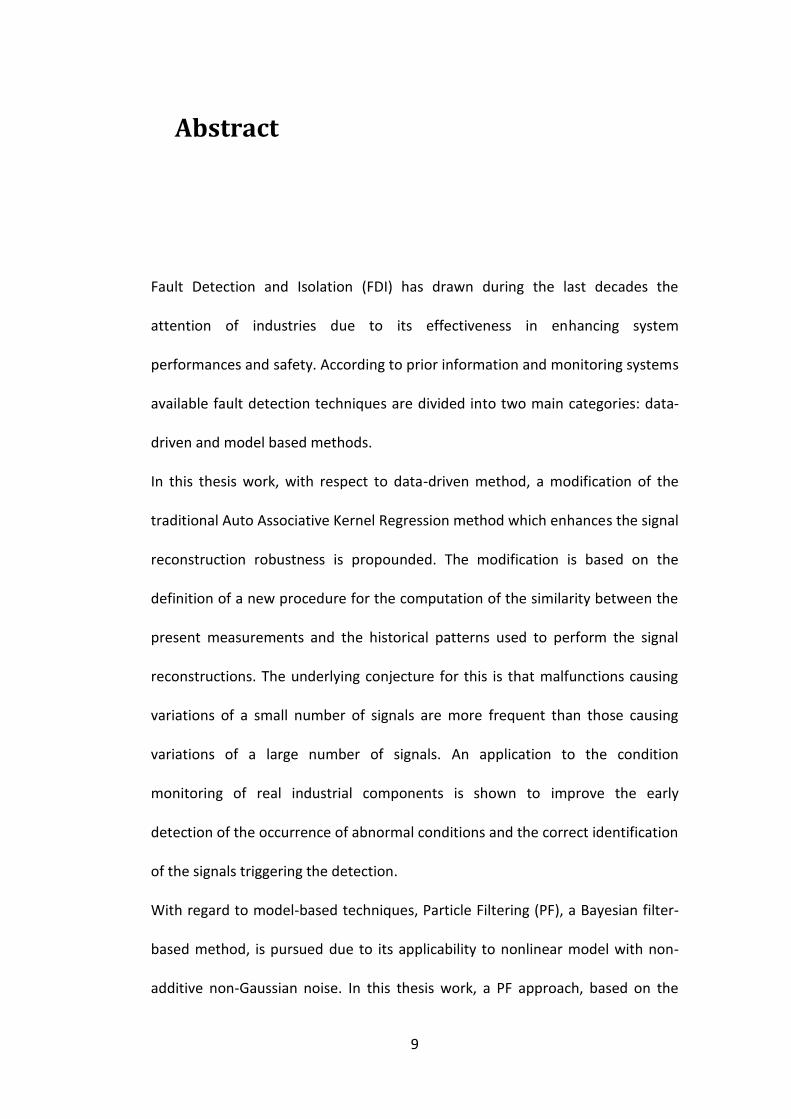
Abstract
Fault Detection and Isolation (FDI) has drawn during the last decades the
attention of industries due to its effectiveness in enhancing system
performances and safety. According to prior information and monitoring systems
available fault detection techniques are divided into two main categories: data-
driven and model based methods.
In this thesis work, with respect to data-driven method, a modification of the
traditional Auto Associative Kernel Regression method which enhances the signal
reconstruction robustness is propounded. The modification is based on the
definition of a new procedure for the computation of the similarity between the
present measurements and the historical patterns used to perform the signal
reconstructions. The underlying conjecture for this is that malfunctions causing
variations of a small number of signals are more frequent than those causing
variations of a large number of signals. An application to the condition
monitoring of real industrial components is shown to improve the early
detection of the occurrence of abnormal conditions and the correct identification
of the signals triggering the detection.
With regard to model-based techniques, Particle Filtering (PF), a Bayesian filter-
based method, is pursued due to its applicability to nonlinear model with non-
additive non-Gaussian noise. In this thesis work, a PF approach, based on the

10
introduction of an augment discrete state pinpointing the particle evolution
model, is propounded to tackle issues where Multiple Models (MM) are available
for the description of the operation of an industrial component in normal and
abnormal conditions. A smooth crack growth degradation problem has been
considered to prove the effectiveness of the proposed method in the detection
of the fault initiation and the identification of the degradation mechanism. The
comparison of the obtained results with that of a literature method and an
empirical statistical test has shown that the proposed method provides both an
early detection of the fault initiation and an accurate identification of the
degradation mechanism. A reduction of the computational cost is also achieved.

11
Sommario
Lo sviluppo negli ultimi decenni di strumentazioni relativamente economiche per
il monitoraggio continuo ha stimolato l’interesse verso piani di manutenzione per
impianti industriali di tipo dinamico. Essi, anziché ricorrere a manutenzioni
programmate, mirano a valutare le condizioni di degrado dei componenti
monitorati e sulla base di quest’ultime decidere se sia utile condurre delle
manutenzioni. L’arresto non necessario di un impianto per sostituire dei
componenti o per eseguire delle manutenzioni può, infatti, comportare alti costi
economici. Nell’affrontare tale tematica sono divenuti essenziali:
l’identificazione di condizioni di funzionamento anomalo;
l’isolamento delle cause del malfunzionamento.
Il contributo che l’Identificazione e Isolamento di Anomalie (IIA) fornisce alle
manutenzioni dinamiche è tale che nel corso degli ultimi decenni il mondo della
ricerca e dell’ industria ha rivolto un elevato interesse verso lo sviluppo di
tecniche sempre più efficaci. Una buona IIA è caratterizzata da una rapida
individuazione delle anomalie e da un’accurata identificazione del processo e
delle cause di degrado ad esse associate. Le tecniche di IIA si possono classificare
in due categorie principali:
metodi basati su modelli espliciti del comportamento del componente.
metodi basati sulle osservazioni storiche (OS) del comportamento del
componente.
In questo lavoro di tesi sono stati sviluppati contributi innovativi in entrambe le
categorie. Generalmente i metodi basati sulle osservazioni storiche identificano
eventuali anomalie nel comportamento del componente ricorrendo a modelli
empirici costruiti con dati storici disponibili.

12
Infatti data un’osservazione i modelli empirici permettono di indentificare un
eventuale guasto. Tale processo si basa sul confronto tra l’osservazione e il
valore ricostruito dal modello, il quale corrispondente al corretto funzionamento
del componente. La modalità con cui viene effettuata la ricostruzione è ciò che
contraddistingue i diversi metodi. Questo lavoro di tesi si è focalizzato
sull’AutoAssociative Kernel Regression (AAKR) che propone una ricostruzione
come media pesata delle osservazioni già raccolte durante condizioni di normale
funzionamento. I pesi possono essere considerati come un indice di similarità tra
il comportamento osservato e l’osservazione storica. In questo studio viene
proposta una modifica all’algoritmo utilizzato per il calcolo dei pesi al fin di
ottenere delle ricostruzioni più robuste. La modifica apportata si basa
sull’introduzione di una proiezione delle osservazioni in un nuovo spazio degli
stati in modo da considerare la maggior frequenza di accadimento di guasti che
coinvolgono un numero ridotto di segnali rispetto a guasti che coinvolgono un
numero maggiore di essi. Il procedimento è stato testato durante il monitoraggio
delle condizioni di alcuni componenti di un impianto di produzione di energia
elettrica. I risultati mostrano come il metodo introdotto sia in grado di
identificare prima del AAKR tradizionale l’occorrenza di anomalie nei
componenti. Inoltre esso è in grado di isolare i sensori che realmente
monitorano l’anomalia del componente, consentendo di eseguire delle
manutenzioni mirate. Infine i costi computazionali sono paragonabili a quelli del
metodo tradizionale, questo permette la sua applicazione a sistemi di
monitoraggio continui..
Per quanto riguarda i metodi basati su modelli espliciti questo lavoro è
focalizzato sul Particle Filtering (PF) poiché consente di trattare modelli espliciti
con un numero di restrizioni molto ridotto rispetto alle altre tecniche già
proposte in letteratura, come il filtro di Kalman e le sue generalizzazioni. In
particolare il PF è in grado di trattare modelli non lineari soggetti a rumori non
additivi e non Gaussiani attraverso l’utilizzo di una distribuzione empirica. In
molti casi il funzionamento o lo stato di degrado di un componente può essere

13
descritto da Modelli Multipli (MM). Generalmente un modello di riferimento è
disponibile per descrivere le condizioni di normalità e diversi modelli per
descrivere i possibili stati di guasto o di degrado. La fase di isolamento in questo
ambito consiste nell’identificare quale sia il modello che maggiormente spiega le
osservazioni raccolte. In letteratura questo problema è già stato affrontato
utilizzando un diverso PF per ogni modello disponibile e andando a identificare a
posteriori quale delle filtrazioni ottenute, quindi l’associato modello, sia la più
adatta ai dati raccolti. D’altro canto tale strategia richiede un grosso sforzo
computazionale dovuto all’elevato numero di particelle da simulare. Per evitare
di simulare diversi gruppi di particelle è stato proposto di introdurre una variabile
discreta indicante esplicitamente il modello secondo il quale esse evolvono. In
questo modo è sufficiente utilizzare un unico PF riducendo quindi il costo
computazionale. Inoltre il PF così ottenuto, durante la fase di aggiornamento
della distribuzione empirica, è in grado di promuovere le particelle che evolvono
secondo il modello più consono all’osservazione raccolta, rendendolo auto
adattativo. Questo consente di isolare il modello più verosimile alle osservazioni
mediante la marginalizzazione della distribuzione empirica sulla variabile discreta
associata ai modelli. La validità di tale metodo è stata testata su un problema di
degrado di un componente sotto sforzo. In particolare si è considerata la
propagazione di una crepa al suo interno, descritta attraverso tre modelli di
degrado non necessariamente lineari e altamente stocastici. Questo è il primo
lavoro, per quanto ne sia a conoscenza l’autore, che tale tipo di approccio venga
applicato ad un problema di diagnostica. I risultati ottenuti mostrano come tale
metodo sia risultato efficace nel rapido riconoscimento del degrado del
componente ed in particolare nel diagnosticare la fase di degrado associata.

14
1
Introduction
In recent years, the development of relatively affordable on-line monitoring
technology has yielded a growing interest in dynamic maintenance paradigms
such as Condition-Based Maintenance (CBM). This is based on tracking the health
conditions of the monitored industrial component and, on this basis, making
maintenance decisions. To do this, two fundamental issues are addressed:
detection, i.e., the recognition of a deviation from the normal operating
conditions;
isolation or diagnostics, i.e., the characterization of the abnormal state of
the component.
In principle, an effective fault detection system is characterize by a prompt
detection of the deviation of the component from the normal conditions of
functioning: the earlier the detection time, the larger the time available to plan
optimal maintenances intervention. This is particularly important for safety
critical components whose failure and malfunctioning can lead to undesired
Introduction
15
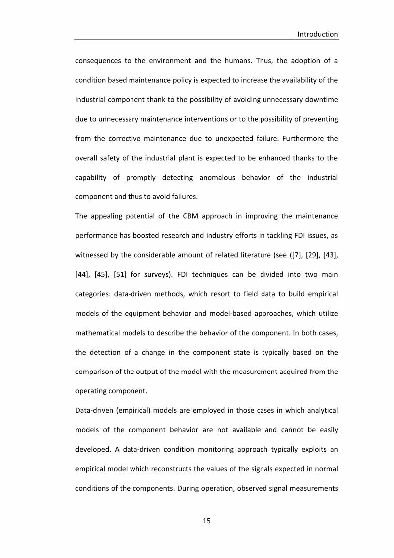
consequences to the environment and the humans. Thus, the adoption of a
condition based maintenance policy is expected to increase the availability of the
industrial component thank to the possibility of avoiding unnecessary downtime
due to unnecessary maintenance interventions or to the possibility of preventing
from the corrective maintenance due to unexpected failure. Furthermore the
overall safety of the industrial plant is expected to be enhanced thanks to the
capability of promptly detecting anomalous behavior of the industrial
component and thus to avoid failures.
The appealing potential of the CBM approach in improving the maintenance
performance has boosted research and industry efforts in tackling FDI issues, as
witnessed by the considerable amount of related literature (see ([7], [29], [43],
[44], [45], [51] for surveys). FDI techniques can be divided into two main
categories: data-driven methods, which resort to field data to build empirical
models of the equipment behavior and model-based approaches, which utilize
mathematical models to describe the behavior of the component. In both cases,
the detection of a change in the component state is typically based on the
comparison of the output of the model with the measurement acquired from the
operating component.
Data-driven (empirical) models are employed in those cases in which analytical
models of the component behavior are not available and cannot be easily
developed. A data-driven condition monitoring approach typically exploits an
empirical model which reconstructs the values of the signals expected in normal
conditions of the components. During operation, observed signal measurements

Introduction
16
are compared with the reconstructions provided by the model: abnormal
components conditions are detected when the reconstructions are remarkably
different from the measurements. Several empirical reconstruction modeling
technique have been applied for condition monitoring of industrial components
such as AutoAssociative Kernel Regression (AAKR [3]), Principal Component
Analysis (PCA [19],[24]), Evolving Clustering Method (ECM), Support Vector
Machine (SVM, [28]) , AutoAssociative (AA) and Recurrent (R) Neural Networks
(NN) ([8],[23],[38],[48]), Local Gaussian Regression (LGR, [35][41]). In this work,
we consider AAKR which has been shown to provide more satisfactory
performance in many cases, has often proven superior to other methods like,
e.g., ECM and PCA [15] and is less computationally demanding than methods,
e.g., AANN and RNN. Notice that small computational cost is an important
desideratum for condition monitoring systems, since they are typically used
online, during component operation and, thus the outcome of the FDI should be
provided to the maintenance decision makers as soon as possible. Applications
of the AAKR method to fault detection in industrial components have been
proposed in [3], [4], [5], [15], [16], [20], [26] and [27]. They have shown the low
robustness of the method in case of abnormal conditions, especially when the
observed signals are highly correlated. By robustness, here we intend the
property such that, in case abnormal or noisy measurements are collected, the
reconstruction of the signal expected in normal condition provided by the
empirical model, is not affected by errors or drift. Low robustness entails a delay
in the detection time and an incorrect identification of the signal impacted by

Introduction
17
abnormal conditions (Fault Isolation). In the first part of the thesis work, a novel
modified AAKR method is presented to overtake these limitations of the
traditional AAKR method. The modification of the AAKR method is based on the
definition of a new procedure for the computation of the similarity between the
present measurements and the historical patterns used to perform the signal
reconstructions. The rationale behind this proposition of the modification is the
attempt to privilege those abnormal conditions caused by the most frequently
expected malfunctions and failures. The performance of the proposed method
will be tested on real data collected from an industrial plant for energy
production.
In the second part of this thesis work, model-based methods which exploit
mathematical models to describe the component behavior in normal and
abnormal conditions, are considered. They usually estimate physical quantities
which are related to the component health state or degradation level. For
example, monitoring of structures can be based on the estimate of the length of
cracks. In particular, a number of filtering algorithms have been successfully
applied to FDI, which use discretized differential equations to describe the
degradation evolution, and stochastic noises to take into account the associated
aleatory uncertainty. For example, Kalman Filter (KF) has been adopted to detect
incidents on freeways [47], and to set a CBM policy on turbine blades affected by
creep [6]. However, KF suffers from a limited applicability, due to the stringent
hypotheses of model linearity and Gaussian noise, which are required and are
often not compatible with practical FDI issues. Thus, some generalizations of KF

Introduction
18
such as Extended Kalman Filter (EKF [36], [37]) and Unscented Kalman Filter
(UFK, [30]) have been proposed to relax the strictness of the KF’s hypotheses.
Nonetheless, there are still situations where these filtering approaches fail, due
to high non linearity or the presence of non-Gaussian noise.
In this framework, Particle Filtering (PF) has drawn the attention of the
researchers due to its wide range of applicability to nonlinear, non-Gaussian
models ([2],[17],[46],[49] and [50]). In particular, PF has been adopted as a FDI
tool within the Multi-Model (MM) systems framework, where the description of
the possible component abnormal evolutions relies on a set of models [31]. In
this setting, detection aims at identifying when the component starts to leave
the nominal model, representing its behavior in normal condition, whereas
diagnostics consists in selecting the model that best fits the current behavior of
the component. The approaches in [1], [12] and [33] are based on the simulation
of parallel swarms of particles according to each operating model and on the
selection, via likelihood analysis between the simulated trajectories and the
gathered measurements, of the model that best fits the observations. However,
this entails an increasing computational cost due to the large number of particles
that must be simulated. A promising approach introduced in ([39], [42])
propound to augment the state vector of the particle with a Boolean variable
concerning the state of health of the component. This allows to take into account
the evolution of the component state avoiding to increase the number of
particles to be simulated. In this thesis work, this idea is applied for the first time,
at the best of the author’s knowledge, to a nonlinear, highly non-Gaussian

Introduction
19
smoothly degradation process of an industrial component subject to an high
measurement error. The case study concerns a component subjected to fatigue
crack growth, whose degradation process can be described by three different
models. The performances obtained by the proposed approach will be compared
with those obtained from a multiple swarms method [12] and from a statistical
sequential test. Furthermore another novel contribution of this thesis work is to
apply this approach for diagnostic, since it has never been exploited for
monitoring components where different type of abnormal behavior can occur.
The objective of the novel method is to provide, at a reduced computational
cost, an early detection of the fault initiation and a prompt identification of the
degradation phase. The remainder of the thesis work is organized as follow: in
Chapter 2, the data-driven FDI is tackled according to the AAKR method. A novel
modified AAKR method is here proposed and applied to a real case study; in
Chapter 3 the Bayesian Filter-Based FDI is proposed. Application to a crack
degradation process and comparison of the results with those obtained from an
MS method is also reported. Finally, Chapter 4 presents the conclusions and
describes the potential future direction of research. In appendix an introduction
to the PF algorithm is presented.

20
2
AutoAssociative Kernel-Based
Data-driven (empirical) models are employed in those cases in which analytical
models of the component behavior are not available and cannot be easily
developed. Data-driven models are built using historical data collected during
operation and require a limited number of hypotheses ([27],[44],[45]). A data-
driven condition monitoring approach is typically based on an empirical model
which reconstructs the values of the monitored signals expected in normal
conditions of the components. During operation, signal measurements are
compared with the reconstructions provided by the empirical model: abnormal
conditions are detected when the reconstructions are remarkably different from
the measurements.
Several empirical reconstruction modeling technique have been applied for
condition monitoring of industrial components ([3],[4],[5],[15],[19],[23] and
[24]). These methods can provide accurate reconstructions of the measured
signals under normal operations, but they often tend to be not robust. By
robustness, here it is intended the property such that, in case abnormal or noisy
measurements are collected, the reconstruction of the signal expected in normal
condition provided by the empirical model, is not affected by error or drift. In [3],
it has been shown that in case of abnormal conditions, empirical models may

AutoAssociative Kernel-Based
21
provide reconstructions of the measured signals which are not estimating the
expected values of the signals in normal conditions, especially when the
measured signals are highly correlated. In particular, it has been shown that the
reconstruction provided by AAKR of an anomalous transient characterized by a
drift of one signal can be not satisfactory for two reasons: 1) the reconstruction
of the signal affected by the drift tends to assume values in the middle between
the drifted and the expected values of the signal in normal conditions 2) the
reconstructions of other signals not affected by the drift tend, erroneously, to be
different from the signal measurements, (this latter effect is usually referred to
with the term ‘spill-over’). The consequence of 1) is a delay in the detection of
abnormal conditions, whereas the consequence of 2) is that the condition
monitoring system, although it correctly triggers an abnormal condition alarm, it
is not able to correctly identify the signal that triggers the alarm.
These limitations of reconstruction models have been already studied in ([3],[15]
and [20]). Solution to these problems have been proposed, which amount to try
to exclude the signals with abnormal behaviors from the set of input signals used
to perform the reconstruction
In ([3], [4] and [16]),the authors have propounded ensembles of reconstruction
models handling different sets of input signals. In case of an anomaly impacting
the behavior of a generic signal, only the few models fed by that signal provide
non robust reconstructions, whereas all the other models provide correct
reconstructions. Another solution has been embraced in [20] whereby a
ponderation matrix iteratively modifies its elements to reduce the contribution
of abnormal signals to the reconstruction but the convergence of the method to
correct signal reconstructions has not been yet demonstrated. All these solution
come at high computational costs.
The objective of this chapter is to propose a robust signal reconstruction method
with low computational cost and i) capable of early detection of abnormal
conditions, ii) accurate in the reconstructions of the values of the signals
impacted by the abnormal conditions and iii) resistant to the spill-over effect.

AutoAssociative Kernel-Based
22
The proposed method is based on the modification of the measure of similarity
used by the Auto-Associative Kernel Regression (AAKR) method. Whereas the
traditional AAKR employs measures of similarity based on Euclidean or
Mahalanobis distances, the proposed method introduces a penalty vector which
reduces the contribution provided by those signals which are expected to be
impacted by the abnormal conditions. The rationale behind this proposition of
the modification is the attempt to privilege those abnormal conditions caused by
the most frequently expected malfunctions and failures. The performance of the
proposed method has been tested on real data collected from an industrial plant
for energy production. The remainder of the chapter is organized as follows.
In Section 2.1, the fault detection problem is introduced. In Section 2.2 the AAKR
method is briefly recalled. Section 2.3 shows the limitation of the traditional
AAKR approach to condition monitoring and states the objectives of the present
chapter. In Section 2.4, the proposed modification of the traditional AAKR is
described and discussed. In Section 2.5, the application of the proposed method
to a real case study concerning the monitoring of 6 signals in an industrial plant
for energy production is discussed. Finally, in Section 2.6 some conclusions are
drawn.

AutoAssociative Kernel-Based
23
2.1 Fault Detection with Empirical Model
In this chapter condition monitoring scheme for fault detection as shown in Fig.
2.1 is considered.
The (empirical) model reproducing the plant behavior in normal conditions
receives in input the vector, , containing the actual observations of the J
signals monitored at the present time, t, and produces in output the
reconstructions, , i.e. the values that the signals are expected to have in
normal conditions. If the actual conditions at the time t are, instead, the
residuals, i.e. the variations between the observation
and the reconstructions, are larger and can be detected by exceedance of a
prefixed thresholds by at least one signal.
Fig. 2.1 Scheme of condition monitoring for fault detection
2.2 AutoAssociative Kernel Regression (AAKR)
The basic idea behind AAKR is to reconstruct at time t the values of the signals
expected in normal conditions, , on the basis of a comparison of the
currently observed signals measurements (also referred to as test pattern),
, and of a set of historical signals
measurements collected during normal condition of operation. In practice, AAKR
performs a mapping from the space of the measurements of the signals
to the space of the values of the signals expected in normal conditions, :
(2.1)

AutoAssociative Kernel-Based
24
where indicates a matrix containing N historical observations of
the signals performed in normal-conditions. Since the mapping is independent
from the present time, t, at which the signals observations are performed, the
present time t will be omitted from the notations. Thus, , =1, …,
indicates the value of signal at the present time. The reconstruction of the
expected values of the signals in normal conditions, ,
is performed as a weighted sum of the available historical observations; for the
generic -th element of , this is:
(2.2)
The weights, , measure the similarity between the test pattern, , and
the -th historical observation vector, . They are evaluated through a
kernel, , i. e., a scalar function which can be written as a dot product. From
the mathematical point of view, a Kernel is a function:
(2.3)
where is a map from the observation space in a (possibly countable infinite
dimensional) Euclidean space and denots the dot product. Traditional
AAKR adopts as function the Gaussian Radial Basis Function (RBF) with
bandwidth parameter , i.e.:
(2.4)
Notice that, according to Mercer’s theorem [10], eq. (2.4) can be seen as a dot
product in a countable infinite dimensional Euclidean space:
(2.5)
In fault detection applications, Euclidean and Mahalanobis distances are typically
used to compute the distance in the Gaussian RBF. In this work, in order to

AutoAssociative Kernel-Based
25
account for differences in the scale and variability of the different signals, a
Mahalanobis distance is used, defined by the covariance matrix, S, such that:
(2.6)
Assuming independence between the signals, is given by:
(2.7)
where indicates the estimated variance of signal j in the historical
observations. Alternatively, instead of using (2.6) and (2.7), one can obtain the
same results by mapping the data in a normalized space according to:
(2.8)
where is the mean value of signal in the historical dataset, and by applying a
Gaussian kernel with Euclidean distance in the normalized space.
2.3 Limitations in the Use of AAKR for Signal
Reconstruction
The availability of relatively affordable monitoring technology typically leads to
the installation of a great number of sensors, which are often monitoring signals
characterized by high degrees of correlation. In this context of correlated signals,
AAKR reconstructions performed in abnormal conditions have been shown to be
not satisfactory from the point of view of the robustness: the obtained
reconstructions are not accurately estimating the values of the signals expected
in normal conditions [4]. This effect is well illustrated by the following case study
concerning the monitoring of a component of a plant for the production of
energy. A dataset containing the real evolution of 6 highly correlated signals
(Table 2.1) for a period of 1 year with sampling frequency of 5200

AutoAssociative Kernel-Based
26
measurements/year has been used to develop an AAKR reconstruction model.
Then, in order to artificially simulate an abnormal condition, a linearly increasing
drift has been added to the real values of one of the six signals for a period of
600 time steps: these drifted data have not been used to develop the AAKR
model. Fig. 2.2 (top) shows the drifted signal, whereas Fig. 2.2 bottom shows the
residuals of the reconstruction of the drifted signal (left) and of another signal
not affected by the abnormal condition (right). Notice that the obtained
reconstructions are not robust: 1) the residuals of the drifted signal are not
following the applied drift 2) the residuals of the other signal is erroneously
deviating from 0.
S1 S2 S3 S4 S5 S6
S1 1 0.97 0.98 0.98 0.99 0.98
S2 0.97 1 0.95 0.99 0.98 0.96
S3 0.98 0.95 1 0.96 0.99 0.99
S4 0.98 0.99 0.96 1 0.98 0.97
S5 0.99 0.98 0.99 0.98 1 0.99
S6 0.98 0.96 0.99 0.97 0.99 1
Table 2.1 degree of correlation between the signals

AutoAssociative Kernel-Based
27
Fig. 2.2 Top (left): the continuous line represents signal 1 values in normal conditions, the dotted line the signal values in the simulated abnormal conditions; top (right): evolution of signal 3 (not affected by the
abnormal conditions). Bottom: the continuous line represents the residuals obtained by applying the traditional AAKR reconstruction, the dotted line the residual which would be obtained by a model able to
perfectly reconstruct the signal behavior in normal conditions.
From the practical point of view of the fault detection, two problems arise in
relation to the low robustness of the reconstruction:
1) delay in the detection of the abnormal condition (an alarm is usually
triggered when the residuals exceed prefixed thresholds).
2) detection of abnormal conditions on signals different from those which
are actually impacted by the abnormal behavior (spill-over).
With regards to the latter, the identification of the signals which are affected by
the abnormal conditions is critical since it can allow to identify the cause of
abnormality and, thus, to properly plan the maintenance intervention.
0 200 400 600 800550
555
560
565
570
575
580
Measure
ment
Normal condition
Simulated abnormal condition
0 200 400 600 800-5
0
5
10
15
Time
Resid
ual
0 200 400 600 800545
550
555
560
565
Measure
ment
0 200 400 600 800-4
-3
-2
-1
0
1
Time
Resid
ual
Normal condition
Traditional AAKR
Simulated residuals
Traditional AAKR
Simulated residuals

AutoAssociative Kernel-Based
28
2.4 Modified AAKR
In order to enhance the AAKR robustness, it is propose to modify the
computation of the weights as the traditional AAKR (eq. (2.4)). The basic ideas
underling the proposed modification are (a) to identify the signals affected by
abnormal behaviors and (b) to reduce their importance in the computation of
the similarity between the test pattern and the historical observations.
With respect to (a), it is assumed that the probability of occurrence of a fault
causing variations on a large number of signals is lower than that of a fault
causing variations on a small number of signals:
if (2.9)
where and indicate the sets of signals affected by variations due
to the abnormal (faulty) conditions, and and their cardinality. If
it is considered, for example, the problem of sensor failures, it is reasonable to
assume that the probability of having N1 faulty sensors at the same time is lower
than that of having an higher number of faulty sensors, N2 < N1, at the same
time. This situation is outlined in Fig. 2.3, where the historical observations
representing the component behavior in normal conditions are represented by
dots and the abnormal condition test pattern by a square. According to the
assumption in eq. (2.9), it is more probable that the abnormal condition is
caused by a failure of a single component (for example, corresponding to normal
conditions close to the pattern in B) than by a simultaneous failure of two
components (corresponding to normal conditions close to the pattern in A).

AutoAssociative Kernel-Based
29
Fig. 2.3 Set of high correlated historical observations (dots) and test pattern (square). A represents the possible reconstruction of the test pattern in the case in which only one component is faulty, B is the case
in which 2 components are faulty.
The proposed procedure computes the similarity measure between the
observation, , and the generic -th historical observation, ,
according to two steps: (a) a pre-processing step consisting in the projection of
and in a new space defined by a penalization vector,
, with increasing entries, i.e., and (b) the
application of the Gaussian RBF kernel in the new space.
Step (a) is based on:
computing the vector of the absolute values of the normalized
differences between and :
(2.10)
defining a permutation matrix, , i.e. a matrix which, when
multiplied to a vector, only modifies the order of the vector
components; in our procedure, we define a matrix, , such
that when it is applied to the vector , the
components of the obtained vector are the same of that of
, but they appear in a decreasing order, i.e.

AutoAssociative Kernel-Based
30
the first component is the one with the largest difference in
;
defining a diagonal matrix having decreasing entries on its
diagonal:
(2.11)
where the vector will be referred
to as penalization vector;
projecting and in a new space defined by the
transformation:
(2.12)
In step (b), we apply to and the Gaussian kernel with
Euclidean distance:
(2.13)
Notice that in this work it is not investigated whether the sequential application
of steps (a) and (b) defines a kernel function according to eq. (2.3). Here, in order
to show the effects of its application, two different historical patterns,
and , are considered, which are characterized by similar
Euclidean distance from a test pattern, but with characterized by a
lower number of signals remarkably different from that of the test pattern. In
this case, the effect of the penalty vector is to assign to an higher
similarity measure than that assigned to . Considering the case of
Fig. 2.3, the similarity of (square) with the pattern in B results higher than
that with the pattern in A, whereas, according to the traditional AAKR pattern A
is more similar than pattern B to the test pattern.
Fig. 2.4 shows the locus of points characterized by the same similarity to the
origin (0,0) in a 2-dimensional space using a penalty vector . The

AutoAssociative Kernel-Based
31
obtained surface is very different from the circle which would be obtained by
using an Euclidean distance. As expected, such modification introduces a
preference during the reconstruction of for that points of that have
deviation on a lower number of components.
Fig. 2.4 2D locus of points having similarity from the origin greater than a set value according to a penalty vector
The application of the proposed method is also exemplified with reference to a
numerical conceptual case study. Let us assume to have available an infinite
dataset of historical data containing all the possible normal conditions of 3
signals with degree of correlation equal to 1, i.e. (
) and to have a test pattern containing the three signal
measurements at the present time. According to the traditional AAKR procedure,
the Euclidean distance between the test pattern and the -th training patterns is:
, which leads to identifying the historical pattern
as the nearest to the test pattern (see Fig. 2.5 and Fig.
2.6). Thus, will be associated to the highest weight, and the signal
reconstruction will be close to it. The reconstruction suggests that there is an
abnormal condition impacting all three signals at the same time. Let us now
consider the reconstruction performed by using the proposed method with a
penalization vector . In this case, the most similar pattern is
AutoAssociative Kernel-Based
32
and the signal reconstruction will be close to it.
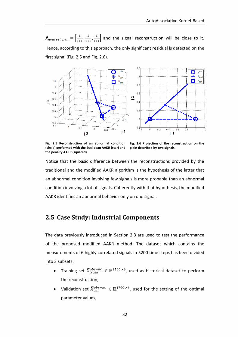
Hence, according to this approach, the only significant residual is detected on the
first signal (Fig. 2.5 and Fig. 2.6).
Fig. 2.5 Reconstruction of an abnormal condition (circle) performed with the Euclidean AAKR (star) and the penalty AAKR (squared).
Fig. 2.6 Projection of the reconstruction on the plain described by two signals.
Notice that the basic difference between the reconstructions provided by the
traditional and the modified AAKR algorithm is the hypothesis of the latter that
an abnormal condition involving few signals is more probable than an abnormal
condition involving a lot of signals. Coherently with that hypothesis, the modified
AAKR identifies an abnormal behavior only on one signal.
2.5 Case Study: Industrial Components
The data previously introduced in Section 2.3 are used to test the performance
of the proposed modified AAKR method. The dataset which contains the
measurements of 6 highly correlated signals in 5200 time steps has been divided
into 3 subsets:
Training set , used as historical dataset to perform
the reconstruction;
Validation set , used for the setting of the optimal
parameter values;

AutoAssociative Kernel-Based
33
Test set, , used for testing the performance of the
method.
In order to verify the performance of the proposed method in case of abnormal
conditions, sensors failures have been simulated in the test set. In practice,
assuming that sensor failures are independent events with probability, (e.g.
=0.2), the following procedure has been applied:
for each signal and each test pattern, a random number, , has been
sampled from an uniform distribution in [0,1]. If < , the sensor is
assumed to be failed and a deviation is simulated from a bimodal
uniform distribution and added to the sensor
measurement.
Thus, the number of signals affected by a deviation in each test pattern is
distributed according to a Binomial distribution . The deviation intensity
has been sampled from the uniform distribution in order
to avoid to confuse the added deviations with the measurement noise which has
been estimated to be a Gaussian noise with standard deviation equal to 1.5.
The obtained test set, , containing both normal and abnormal conditions
patterns, , has been used to verify the performance of the traditional
AAKR method and the modified AAKR with different choices of penalization
vector:
Linear ;
Exponential ;
Cliff Diving Competition ranking 8 20 50 90 160 350 .
In all cases, the optimal bandwidth parameter, , has been identified by
minimizing the Mean Square Error (MSE) of the reconstructions on the validation
set, :
(2.14)

AutoAssociative Kernel-Based
34
Then, for each test pattern, , of , with , the
reconstruction of the signals values expected in normal conditions has
been performed, and the residuals computed. Finally, if , for
, an abnormal condition involving signal is detected.
In order to evaluate the performance in the reconstruction, notice that 4
different possible cases for each test pattern are considered:
1) presence of both false and missed alarms. There is at least one signal for
which an abnormal condition is erroneously detected ( ) when
no sensor failure has been simulated (false alarm) and, at the same time,
at least one signal for which an abnormal condition is erroneously not
detected ( ), when actually a sensor failure has been simulated
(missed alarm);
2) presence of only a false alarm. At least one false alarm, no missing
alarms;
3) presence of only a missed alarm. At least one missed alarm, no false
alarms;
4) correct identification (OK). Neither false nor missing alarms.
Table 2.2 reports the performance of the traditional and modified AAKR
reconstruction methods in terms of fraction of test patterns in which the
application of the detection scheme leads to one of the four categories (1-4),
considering different choices of the penalization vector. For the cases of
exponential and linear penalization vectors, only the results obtained for =10
and =8, which correspond to the best performance, are reported.
PENALIZATION
VECTOR OK
MISSED
ALARMS
FALSE
ALRAMS
MISSED AND
FALSE ALARMS
MODIFIED AAKR EXPONENTIAL = 10 0.885 0.089 0.008 0.018
MODIFIED AAKR DIVING COMPETITION
RANKING 0.669 0.300 0.001 0.030
MODIFIED AAKR LINEAR = 8 0.585 0.375 0.001 0.039
AutoAssociative Kernel-Based
35
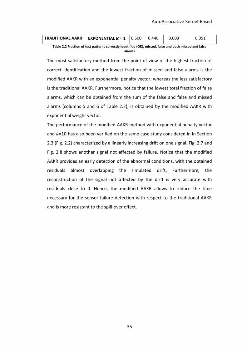
TRADITIONAL AAKR EXPONENTIAL = 1 0.500 0.446 0.003 0.051
Table 2.2 Fraction of test patterns correctly identified (OK), missed, false and both missed and false alarms
The most satisfactory method from the point of view of the highest fraction of
correct identification and the lowest fraction of missed and false alarms is the
modified AAKR with an exponential penalty vector, whereas the less satisfactory
is the traditional AAKR. Furthermore, notice that the lowest total fraction of false
alarms, which can be obtained from the sum of the false and false and missed
alarms (columns 5 and 6 of Table 2.2), is obtained by the modified AAKR with
exponential weight vector.
The performance of the modified AAKR method with exponential penalty vector
and =10 has also been verified on the same case study considered in in Section
2.3 (Fig. 2.2) characterized by a linearly increasing drift on one signal. Fig. 2.7 and
Fig. 2.8 shows another signal not affected by failure. Notice that the modified
AAKR provides an early detection of the abnormal conditions, with the obtained
residuals almost overlapping the simulated drift. Furthermore, the
reconstruction of the signal not affected by the drift is very accurate with
residuals close to 0. Hence, the modified AAKR allows to reduce the time
necessary for the sensor failure detection with respect to the traditional AAKR
and is more resistant to the spill-over effect.

AutoAssociative Kernel-Based
36
Fig. 2.7 Residual of the drifted signal
Fig. 2.8 Residual of a signal not affected by any drift
Further analyses have been performed in order to identify the sensitivity of the
modified AAKR method to the setting of the exponential penalty vector
parameter, to the number of simultaneous sensor failures and to the intensity of
the failure.
100 200 300 400 500 600-6
-5
-4
-3
-2
-1
0
1
Time
Resid
ual
Modified AAKR
Traditional AAKR
Simulated residuals
AutoAssociative Kernel-Based
37
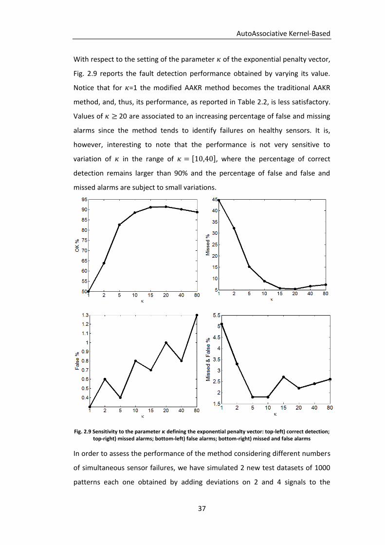
With respect to the setting of the parameter of the exponential penalty vector,
Fig. 2.9 reports the fault detection performance obtained by varying its value.
Notice that for =1 the modified AAKR method becomes the traditional AAKR
method, and, thus, its performance, as reported in Table 2.2, is less satisfactory.
Values of 20 are associated to an increasing percentage of false and missing
alarms since the method tends to identify failures on healthy sensors. It is,
however, interesting to note that the performance is not very sensitive to
variation of in the range of , where the percentage of correct
detection remains larger than 90% and the percentage of false and false and
missed alarms are subject to small variations.
Fig. 2.9 Sensitivity to the parameter defining the exponential penalty vector: top-left) correct detection; top-right) missed alarms; bottom-left) false alarms; bottom-right) missed and false alarms
In order to assess the performance of the method considering different numbers
of simultaneous sensor failures, we have simulated 2 new test datasets of 1000
patterns each one obtained by adding deviations on 2 and 4 signals to the

AutoAssociative Kernel-Based
38
normal condition measurements, respectively. The obtained results are reported
in Table 2.3. The modified AAKR method tends to perform remarkably better
than the traditional AAKR method in the cases of two simultaneous sensor
failures. However, the performance of the two methods tends to decrease if the
number of simultaneous sensor failures increases. In particular, in the case of
four simultaneous sensor failures, the traditional AAKR method performance is
slightly more satisfactory than that of the modified method. This is due to the
consequences of the modified AAKR method hypothesis that signal behaviors
characterized by several signals affected by abnormal conditions are expected to
be rare and so the number of missed alarms increases. This can be explained by
considering the same numerical conceptual case study discussed in Section 2.3.
Let us assume that we have to reconstruct the test pattern which
is characterized by a failure of sensors 1 and 2 (normal condition measurements
would be ). Considering a training set made of patterns (
), the traditional AAKR reconstructs the test pattern in
the neighborhood of
, which is the closest training pattern using an
Euclidean distance, whereas the modified AAKR with penalty vector
reconstructs it in the neighborhood of
. Hence, the
traditional AAKR method detects an anomaly on all the three sensors, providing
a false alarm on sensor 3, whereas the modified AAKR detects a failure on sensor
1, providing a false alarm on sensor 1 and missed alarms on sensors 2 and 3. In
general, it seems that the performance of the modified AAKR is satisfactory
when the total number of sensor failures is lower than half of the number of
sensors
].
2 Simultaneous Errors
OK MISSED FALSE MISSED & FALSE
Traditional AAKR 335 577 9 79
Exponential = 10 837 158 2 3
Table 2.3 Quantitative results for 2 simultaneous error
AutoAssociative Kernel-Based
39
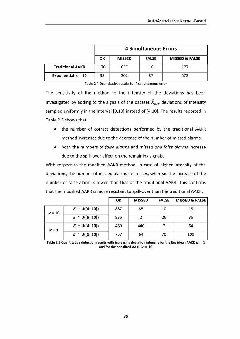
4 Simultaneous Errors
OK MISSED FALSE MISSED & FALSE
Traditional AAKR 170 637 16 177
Exponential = 10 38 302 87 573
Table 2.4 Quantitative results for 4 simultaneous error
The sensitivity of the method to the intensity of the deviations has been
investigated by adding to the signals of the dataset deviations of intensity
sampled uniformly in the interval [9,10] instead of [4,10]. The results reported in
Table 2.5 shows that:
the number of correct detections performed by the traditional AAKR
method increases due to the decrease of the number of missed alarms;
both the numbers of false alarms and missed and false alarms increase
due to the spill-over effect on the remaining signals.
With respect to the modified AAKR method, in case of higher intensity of the
deviations, the number of missed alarms decreases, whereas the increase of the
number of false alarm is lower than that of the traditional AAKR. This confirms
that the modified AAKR is more resistant to spill-over than the traditional AAKR.
OK MISSED FALSE MISSED & FALSE
= 10 Ei ~ U([4, 10]) 887 85 10 18
Ei ~ U([9, 10]) 936 2 26 36
= 1 Ei ~ U([4, 10]) 489 440 7 64
Ei ~ U([9, 10]) 757 64 70 109
Table 2.5 Quantitative detection results with increasing deviation intensity for the Euclidean AAKR and for the penalized AAKR

AutoAssociative Kernel-Based
40
2.6 Conclusion
In this chapter, the condition monitoring of an industrial component has been
considered within a data-driven setting. In order to obtain robust reconstructions
of the values of the monitored signals expected in normal conditions, it has been
proposed to modify the traditional AAKR method. The modification is based on a
different procedure for the computation of the similarity between the present
and the historical measurements collected in normal condition of operation. In
particular, before the computation of the Kernel between the two vectors, which
is performed as in the traditional AAKR method according to a Gaussian RBF
function, the data are projected into a new signal space defined by using a
penalization vector which reduces the contribution of signals affected by
malfunctioning. The procedure is based on the hypothesis that the probability of
occurrence of a fault causing variations on a large number of signals is lower than
that of one causing variations on a small number of signals.
The modified AAKR method has been applied to a real case study concerning the
monitoring of 6 highly correlated signals in an industrial plant for energy
production. The possibility of detecting sensor faults has been investigated. The
obtained results have shown that the reconstructions provided by the modified
AAKR are more robust than those obtained by using the traditional AAKR. This
causes a reduction in the time necessary to detect abnormal conditions and in a
more accurate identification of the signals actually affected by the abnormal
conditions.
41
3
Bayesian Filter-Based Fault Detection
With regards to the model-based approaches, a number of filtering algorithms
have been successfully applied to FDI, which use discretized differential
equations to describe the state evolution, and stochastic noises to take into
account the associated aleatory uncertainty([6], [30], [36], [37] and [47]).
However the high complexity of real industrial system demand for method
capable of manage nonlinear non-Gaussian models, since there are still
situations where traditional filtering techniques fail. In this context, Particle
Filtering (PF) has proven to be a robust technique ([2],[17]) which allows tackling
more realistic FDI problems([46],[49] and [50]). In particular, PF has been
adopted as a FDI tool within the Multi-Model (MM) systems framework, where
the description of the possible abnormal evolutions of the component behavior
relies on a set of models [31]. In this setting, detection aims at identifying when
the behavior of the component starts to leave the nominal mode, whereas
diagnostics consists in selecting the model that best fits in describing the current
behavior of the component.
Interesting applications of PF to FDI in MM systems have been proposed in [1]
and [12], where multiple swarms of particles are contemporaneously simulated,
according to all the possible alternative models. There, FDI are based on Log-

Bayesian Filter-Based Fault Detection
42
Likelihood Ratio (LLR) tests, which exploit the gathered measures to estimate, for
every swarm, the corresponding likelihood of being the right model to track the
observed component behavior. However, these methods are computationally
burdensome and memory demanding, as they require tracing a large number of
particles.
Alternatively, an approach based on the augmentation of the state vector with a
variable representing the model to be selected to describe the current evolution
has been propounded in [39] and [42]. This allows the filter to automatically
convey the particles to follow the right model when the gathered measures force
the state vector to modify the value of the added variable.
In particular, such variable is chosen continuous in [32], which proposes an
ensemble of Monte Carlo adaptive filters, and uses the LLR tests to make the FDI
decision. On the contrary, it is a Boolean variable in [39] and [46], where explicit
fault models with associated fault probabilities are supposed to be known. These
are used to compel the particles to evolve according to the different models.
Then, the measures acquired at the updating steps will favor the particles of the
correct model, i.e., those associated to the correct value of the added variable,
which are expected to be more close to the measured degradation value.
On the other side, the works of the literature which investigate the potential of
such algorithm ([39] and [46]) addressed case studies where only two models are
available, the noise is Gaussian, and the occurrence of a fault reflects in a sharp
jump of the traced degradation variable. These hypotheses may be unrealistic,
especially for continuously degrading components [14]. In this context, the
novelty introduced in this chapter, is to apply PF to FDI in MM systems where
more than two models are available, the noise in the models is not Gaussian and
the degradation process are smoothly evolving. The performances of the
proposed approach are compared with those of both the LLR-based approach
(e.g. [12]), and an intuitive approach based on the statistical hypothesis test
technique.

Bayesian Filter-Based Fault Detection
43
To this aim, a non-linear crack growth degradation process is considered as case
study, which is investigated in two different settings:
1) There are only two models available, one for normal conditions and the
other for degradation; hence, detection and diagnosis coincide. This is the
same setting of other works of the literature (e.g. [39], [46])
2) A third degradation model is considered, in order to evaluate the
diagnostic capability of the proposed approach in selecting the right
model to describe the current evolution behavior.
The remainder of the chapter is organized as follows. In Section 3.1, a general
description of the Multi Model setting is presented, with a focus on the case
study considered in this chapter. In Section 3.2, basics of Particle Filtering are
recalled. Section 3.3 summarizes the characteristics of the PF-based techniques
proposed in the literature to address FDI in Multi Model systems, and describes
the FDI technique based on the augmented state vector. Section 3.4 shows the
application of these FDI methods to the simulated realistic case study of the
crack growth degradation process. Section 3.5 reports some conclusions.
Bayesian Filter-Based Fault Detection
44
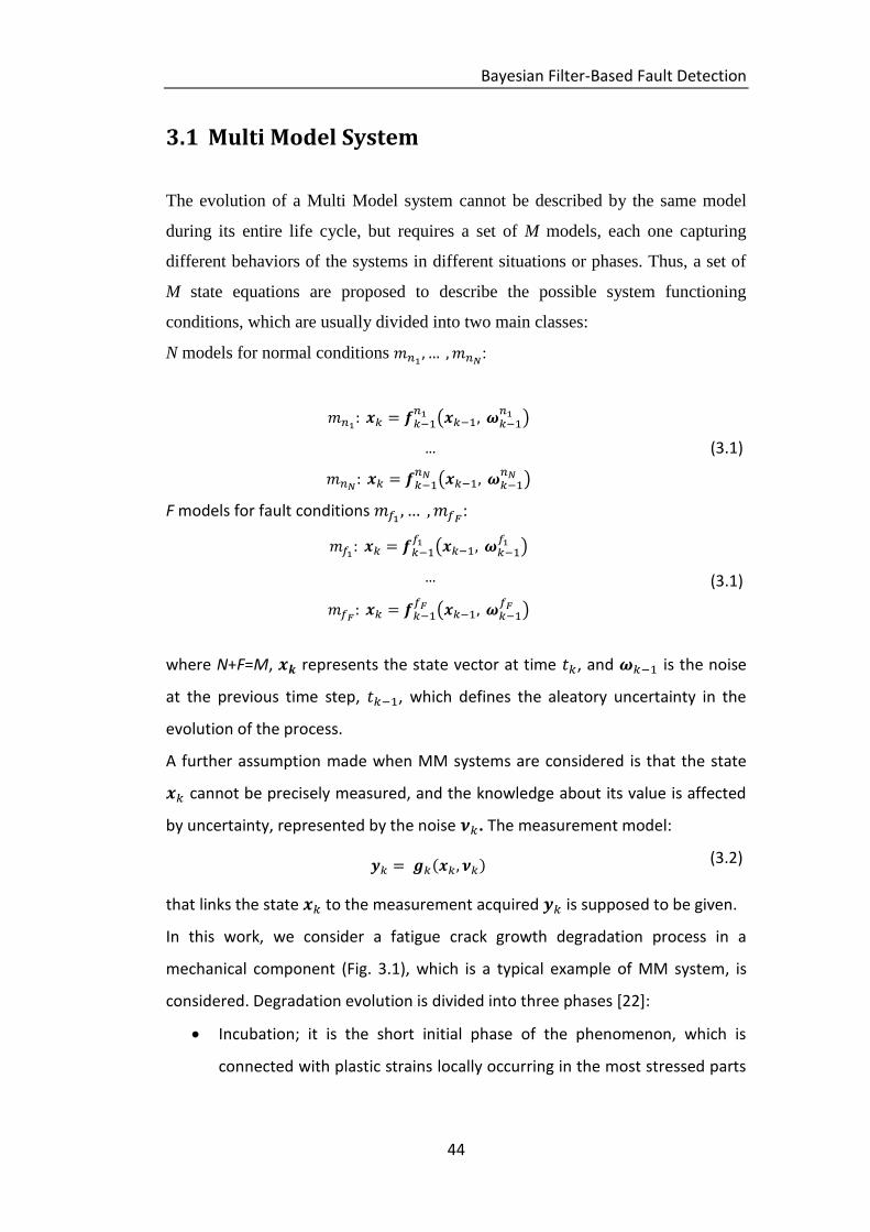
3.1 Multi Model System
The evolution of a Multi Model system cannot be described by the same model
during its entire life cycle, but requires a set of M models, each one capturing
different behaviors of the systems in different situations or phases. Thus, a set of
M state equations are proposed to describe the possible system functioning
conditions, which are usually divided into two main classes:
N models for normal conditions
:
…
(3.1)
F models for fault conditions
:
…
(3.1)
where N+F=M, represents the state vector at time , and is the noise
at the previous time step, , which defines the aleatory uncertainty in the
evolution of the process.
A further assumption made when MM systems are considered is that the state
cannot be precisely measured, and the knowledge about its value is affected
by uncertainty, represented by the noise . The measurement model:
(3.2)
that links the state to the measurement acquired is supposed to be given.
In this work, we consider a fatigue crack growth degradation process in a
mechanical component (Fig. 3.1), which is a typical example of MM system, is
considered. Degradation evolution is divided into three phases [22]:
Incubation; it is the short initial phase of the phenomenon, which is
connected with plastic strains locally occurring in the most stressed parts

Bayesian Filter-Based Fault Detection
45
of the mechanical component subject to cyclic loads. At this stage,
coalescence of dislocations and vacancies, as well as ruptures due to local
stresses lead to the formation of sub-microcracks in the slip bands at the
boundaries of blocks, grains and twins. From the practical point of view,
this phase is modeled by a constant model in which the crack length is
zero, being its exact value not measurable by traditional measurement
instrumentation.
Crack initiation; it is characterized by the growth and coalescence of the
sub-microcracks, which transform into micro-cracks. These start
increasing under the cyclic loads, and form macro-cracks, which are
typically detectable by measurement instrumentation. This gives rise to
the third phase. The model describing this second phase is linear in time
[9].
Crack rapid-propagation; the crack grows under the cyclic loads, up
reaching a critical threshold. A number of models have been proposed to
describe this latter phase, such as the Paris-Erdogan exponential law [40],
here considered.
The measures gathered to monitor the degradation process are affected by
errors, especially during the second phase or when the crack cannot be directly
measured due to its position. In this setting, detection consists in the
identification of the deviation from the first phase, while diagnostics consists in
determining whether the growth is linear (i.e., the second phase) or exponential
(i.e., the third phase).

Bayesian Filter-Based Fault Detection
46
Fig. 3.1 Schematic approximation of the crack propagation model.
3.2 Particle Filtering
Particle Filtering (PF) is a sequential Monte-Carlo method, which is made up of
two subsequent steps: prediction and updating. At time , the prediction of
the equipment state at the next time instant , is performed by considering a
set of weighted particles, which evolve independently on each other,
according to the given probabilistic degradation model (i.e., one out of those in
Eqs. (3.1)). The underlying idea is that such group of weighted random samples
provides an empirical discrete approximation of the true Probability Density
Function (pdf) of the system state conditional on the last
available measure. When a new measure is acquired, it is used to update the
proposed pdf in a Bayesian prospective, by adjusting the weights of the particles
on the basis of their likelihood of being the correct value of the system state. For
practical purpose, PF works as if the i-th particle, i=1, 2, … were the real
system state; then, the smaller the probability of observing the last collected
measurement, the larger the reduction in the particle’s weight. On the contrary,
when the acquired measure well matches with the particle position, then its
importance is increased. Such updating step of the particle weights is driven by
the probability distribution (which is derived from Eq. (3.2)) of
observing the sensors output given the true degradation state , and
provides the distribution .

Bayesian Filter-Based Fault Detection
47
The PF scheme used in this work is the Sequential Importance Resampling (SIR, ,
[2], [17]), which builds a new population of particles by sampling with
replacement from the set of particles
; the chance of a particle being
picked is proportional to its weight. The final weight assigned to the particles of
such new set is
. The SIR algorithm allows avoiding the degeneracy
phenomenon (i.e., after few iterations, all but few particles would have negligible
weights), which is typical of the standard version of PF (i.e., Sequential
Importance Sampling, SIS).
Finally, the updated particle distribution is used to perform the successive
prediction steps up to next measurement (for further theoretical details see [2],
[17], [18] and [34]).
3.3 Particle Filter for Fault Detection and Diagnosis in
Multi Model System.
PF has been already applied to tackle FDI issues in the framework of MM
systems. For example, in [31] PF is used to simultaneously run swarms of
particles evolving according to every possible model (Fig. 3.2). Then, a residual’s
analysis or a Log-Likelihood Ratio (LLR) test is performed to identify the swarm
that best matches with the gathered measure, and thus the corresponding
model. For example, Fig. 3.2 shows the case in which three different swarms are
traced by PF, according to three available models , and . Model is
the best model to represent the system evolution in its first phase, being very
good the matching of the corresponding particle swarm and the measures
acquired at time instants . On the contrary at time the model which
best fits the measures becomes .
Enhancements of this approach have been proposed in [1] and [12]. In the
former work, a new way to estimate the likelihood function is introduced to
extend the applicability of the method to more complex particle distributions. In
Bayesian Filter-Based Fault Detection
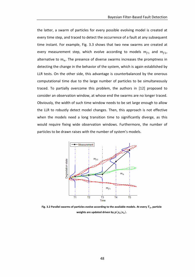
48
the latter, a swarm of particles for every possible evolving model is created at
every time step, and traced to detect the occurrence of a fault at any subsequent
time instant. For example, Fig. 3.3 shows that two new swarms are created at
every measurement step, which evolve according to models and ,
alternative to . The presence of diverse swarms increases the promptness in
detecting the change in the behavior of the system, which is again established by
LLR tests. On the other side, this advantage is counterbalanced by the onerous
computational time due to the large number of particles to be simultaneously
traced. To partially overcome this problem, the authors in [12] proposed to
consider an observation window, at whose end the swarms are no longer traced.
Obviously, the width of such time window needs to be set large enough to allow
the LLR to robustly detect model changes. Then, this approach is not effective
when the models need a long transition time to significantly diverge, as this
would require fixing wide observation windows. Furthermore, the number of
particles to be drawn raises with the number of system’s models.
Fig. 3.2 Parallel swarms of particles evolve according to the available models. At every , particle
weights are updated driven by .

Bayesian Filter-Based Fault Detection
49
Fig. 3.3 At every time step, new swarms of particles start according to the alternative models.
A different way to tackle the MM problems is that of augmenting the state
vector with a new discrete variable, which represents the evolution model of the
system. That is, the state vector becomes , and the degradation
models in eq. (3.1) are embedded in the model:
(3.3)
where encodes also the probabilistic model governing the transitions among
the different possible models, which is a first-order Markov [46].
This setting requires modifications to the PF algorithm. In details, the PF
prediction step has to give due account to the possible alternative models
according to which the particles are simulated:
(3.4)
In the last equation, it has been assumed that the transition probabilities
do not depend on the current degradation state , whereas the
prediction of the state depends on the added variable , whose value is
sampled at the current time instant .

Bayesian Filter-Based Fault Detection
50
The successive updating step at time acts on the distribution of only, since
the acquired measures concern the value of the degradation state , and not
that of the variable . Nonetheless, favoring the particles positioned in the
neighborhood of the measure leads to the selection of the particles with the
most likely value of .
For the sake of clarity, the transition probabilities in (3.4) can be
arranged in the matrix:
(3.5)
where the i-th element of the j-th column represents the probability that a
particle which has been simulated according to model i, will be simulated at the
next step according to model j.
For example, in the case in which there are M=2 alternative models, model 1
refers to the normal state (N=1), whereas model 2 to the failed state (F=1). Then,
is the probability that a particle which at the previous step has been
simulated according to model 1, will be simulated again according to the same
model 1, whereas is the opposite case, i.e., the same particle will change its
stochastic behavior. Fig. 3.4 gives a pictorial view of this dynamics.
Fig. 3.4 Possible transitions among the operational models of the system.
Notice that the transition from model to model , , may be physically
meaningless when it is not possible that a system spontaneously recovers by
itself. However, in the considered setting a positive value is always given to the
corresponding probabilities. In fact, if these were set to zero, the system would
be biased to follow the degraded models especially in case of outlier measure

Bayesian Filter-Based Fault Detection
51
values, as the trajectories of those particles that are erroneously following a
failure model could no longer be corrected.
For the sake of clarity, an example of the dynamic behaviors of the particles
when the measures are gathered from the normal operating system is given in
Fig. 3.5. At time , some particles change their reference model according to
. In particular, some particles experienced a change of the variable from
to . These particles are strongly un-favored at the updating step, being the
acquired measure far from their positions. Thus, among the particles with state
parameter , only few particles (one in Fig. 3.5) are re-sampled and still follow
the wrong model at the next time step, whereas the others are reset to the
starting point. The behavior of the augmented MM PF in the opposite case, i.e.,
when measurements are gathered from a failed system, is shown in Fig. 3.6.
There, during the updating and re-sampling steps, the number of particles having
as augmented state increases. Hence, the measures acquired promote the
particles associated to the correct model, i.e., those labeled with the correct
value of the added variable, which are more close to the measured
degradation value. This allows the particles to auto-adapt their trajectories to
the real evolution of the system, and thus selecting the correct model.
Fig. 3.5 Evolution of a system as long as measurements support the normal model.
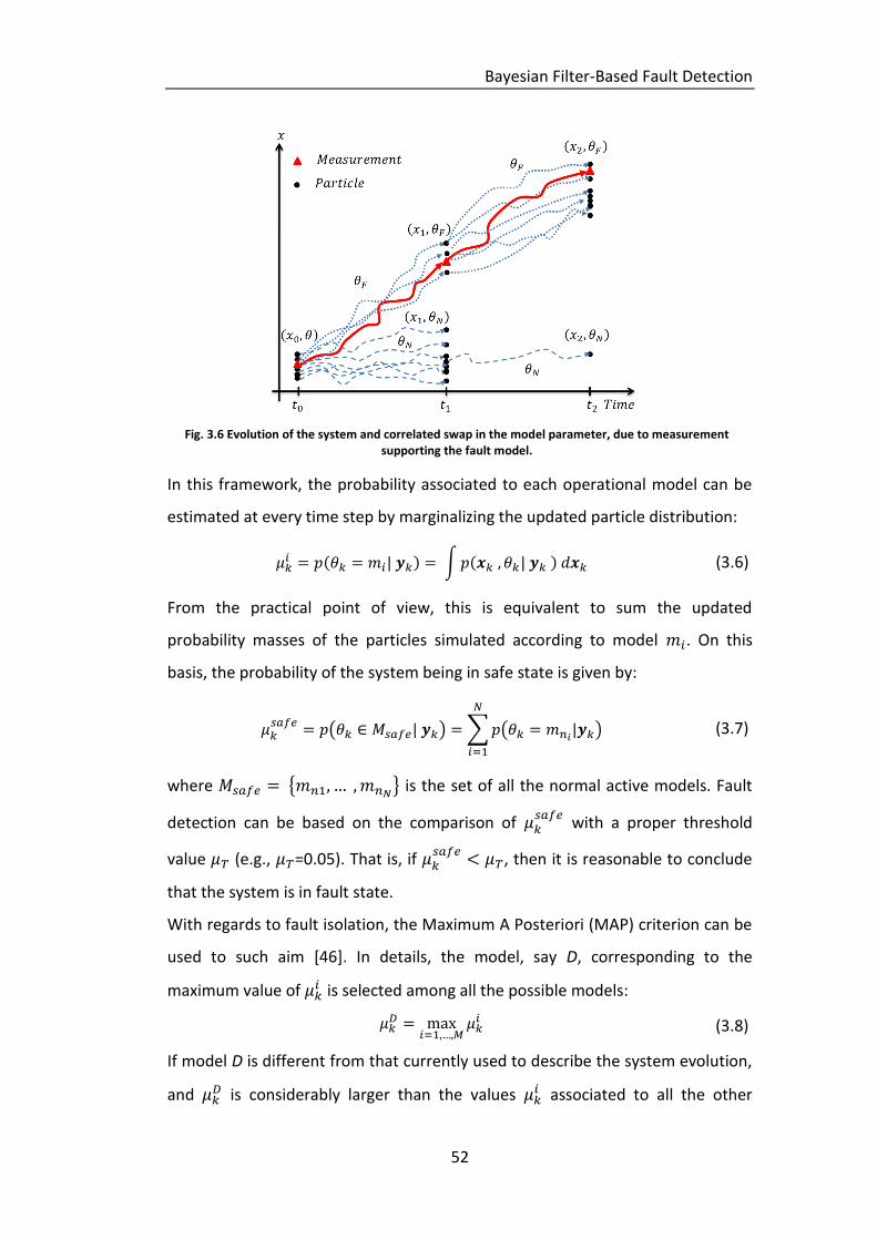
Bayesian Filter-Based Fault Detection
52
Fig. 3.6 Evolution of the system and correlated swap in the model parameter, due to measurement supporting the fault model.
In this framework, the probability associated to each operational model can be
estimated at every time step by marginalizing the updated particle distribution:
(3.6)
From the practical point of view, this is equivalent to sum the updated
probability masses of the particles simulated according to model . On this
basis, the probability of the system being in safe state is given by:
(3.7)
where is the set of all the normal active models. Fault
detection can be based on the comparison of
with a proper threshold
value (e.g., =0.05). That is, if
, then it is reasonable to conclude
that the system is in fault state.
With regards to fault isolation, the Maximum A Posteriori (MAP) criterion can be
used to such aim [46]. In details, the model, say D, corresponding to the
maximum value of is selected among all the possible models:
(3.8)
If model D is different from that currently used to describe the system evolution,
and is considerably larger than the values
associated to all the other

Bayesian Filter-Based Fault Detection
53
models, then a change in the system state is diagnosed. In this respect, to make
more robust decisions and reduce the number of false alarms, one can require
that this criterion is fulfilled for a number of consecutive time steps.
Finally notice that for the sake of generality, in the model considered in (3.3) the
stochastic noise depends not only on time, but also on the value of , i.e.,
on the operating model; this allows giving due account to the different variability
of the alternative models. For example, if the amount of information about the
normal system functioning is larger than that about a failure model, then the
corresponding noise ,
is expected to have
higher variability than ,
.
3.4 CASE STUDY:
Crack Degradation Process
As mentioned in Section 3.1, the case study considered in this work deals with
the crack growth degradation process. The FDI performance of the method that
relies on the augmented state (which is here labeled as IMM, according to the
terminology used in [46]) is evaluated in two different settings:
1) There are only two models available, one for normal conditions and the
other for degradation; hence, detection and diagnosis coincide. This is the
same setting of other works of the literature (e.g., [39], [42]). Then, the
performance of the IMM method is compared with those of the LLR-
based method proposed in [12] (which is here referred to as Multiple
Swarms (MS)) and of an intuitive, statistical approach.
2) A third degradation model is considered, in order to evaluate the
diagnostic capability of the proposed approach in selecting the right
model to describe the current evolution behavior.

Bayesian Filter-Based Fault Detection
54
3.4.1 Two-Model Setting: Fault Detection
3.4.1.1 Model Description
The crack growth evolution is here described as a two phase process:
1) crack incubation, which is modeled by a constant null value, since crack is
too small to be measured:
(3.9)
2) crack propagation, which is modeled by the Paris-Erdogan model [40]:
(3.10)
where describes the uncertainty in the growth speed;
and are parameters related to the component
material, and is an experimentally determined constant related to
the characteristics of the load and the position of the crack. The values of
these parameters are derived from [11], whereas the discretized time
unit is here assumed to be expressed in arbitrary units of time.
The measurement model is:
(3.11)
where is an additive Gaussian measurement error. The
measurement instrument is assumed to have a resolution ,
which means that it is not capable of observing cracks with length
.
To conclude, Fig. 3.7 shows a possible crack evolution and the associated
measures.

Bayesian Filter-Based Fault Detection
55
Fig. 3.7 Crack growth simulation of a crack started at h.
3.4.1.2 Interacting Multiple Model (IMM)
The transition probability matrix for the model parameter has been chosen
as:
(3.12)
where the probabilities of particles changing the reference model are set, at a
first attempt, to very small values, i.e., . This is justified by the
following considerations:
a) with regards to , the larger its value the larger the expected
numbers of particles that start evolving according to the fault
model. For example, if the number of particles is set to
, then on average at every time step a particle of the
swarm is forced to swap model. This entails that when a measure
is acquired from a safe system, the particles with augmented
variable set to are unlikely to be re-sampled, and the swarm
continues evolving in the correct way. On the contrary, if the
probability were set to a larger value, e.g., 0.2, there would be
20 particles evolving according to the fault model. This means that
the probability of having a particle re-sampled from this set
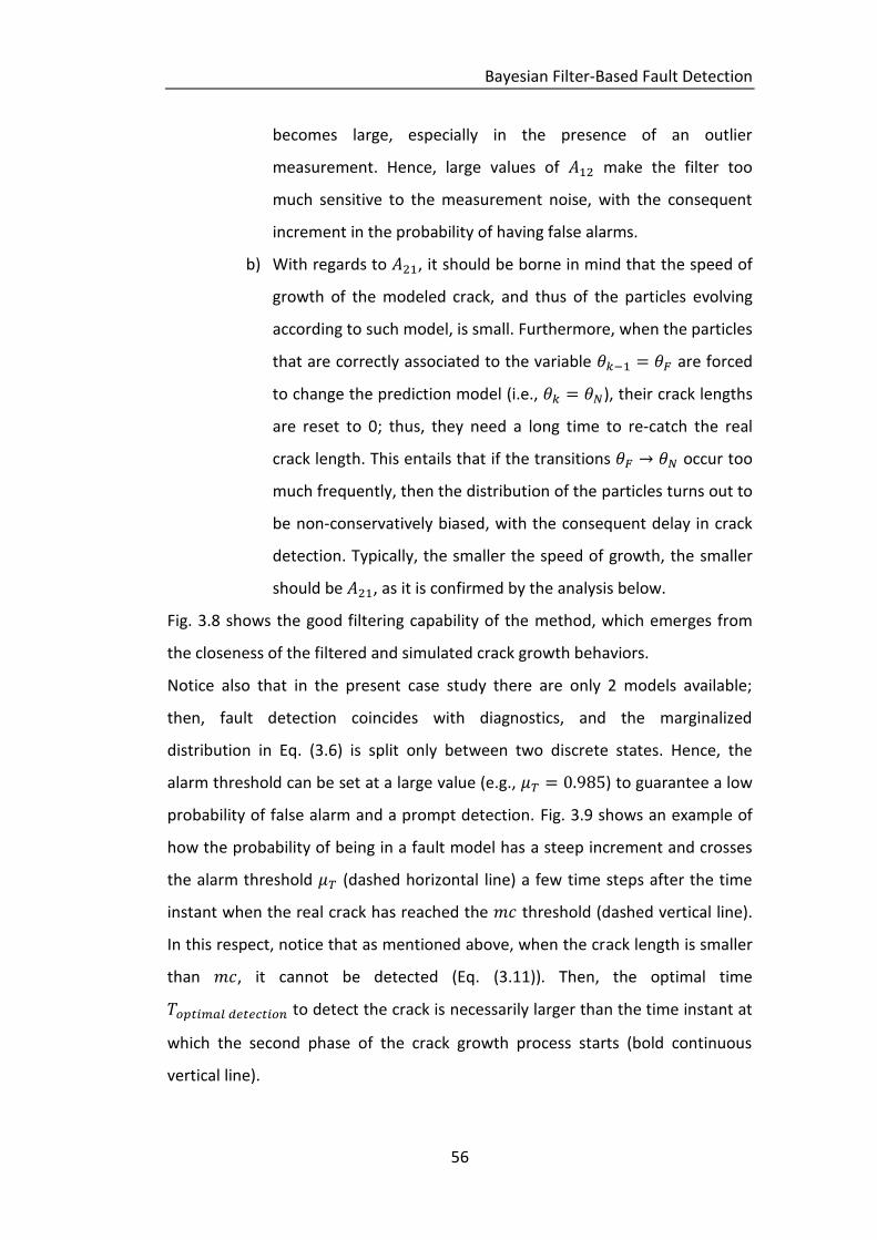
Bayesian Filter-Based Fault Detection
56
becomes large, especially in the presence of an outlier
measurement. Hence, large values of make the filter too
much sensitive to the measurement noise, with the consequent
increment in the probability of having false alarms.
b) With regards to , it should be borne in mind that the speed of
growth of the modeled crack, and thus of the particles evolving
according to such model, is small. Furthermore, when the particles
that are correctly associated to the variable are forced
to change the prediction model (i.e., ), their crack lengths
are reset to 0; thus, they need a long time to re-catch the real
crack length. This entails that if the transitions occur too
much frequently, then the distribution of the particles turns out to
be non-conservatively biased, with the consequent delay in crack
detection. Typically, the smaller the speed of growth, the smaller
should be , as it is confirmed by the analysis below.
Fig. 3.8 shows the good filtering capability of the method, which emerges from
the closeness of the filtered and simulated crack growth behaviors.
Notice also that in the present case study there are only 2 models available;
then, fault detection coincides with diagnostics, and the marginalized
distribution in Eq. (3.6) is split only between two discrete states. Hence, the
alarm threshold can be set at a large value (e.g., ) to guarantee a low
probability of false alarm and a prompt detection. Fig. 3.9 shows an example of
how the probability of being in a fault model has a steep increment and crosses
the alarm threshold (dashed horizontal line) a few time steps after the time
instant when the real crack has reached the threshold (dashed vertical line).
In this respect, notice that as mentioned above, when the crack length is smaller
than , it cannot be detected (Eq. (3.11)). Then, the optimal time
to detect the crack is necessarily larger than the time instant at
which the second phase of the crack growth process starts (bold continuous
vertical line).

Bayesian Filter-Based Fault Detection
57
Notice also that the spike highlighted in Fig. 3.9 is due to an outlier measure,
which could be considered as an observation acquired from a system with no
crack. Nevertheless, the method shows its robustness, being the spike not
capable to force a change in the model identification.
Fig. 3.8 Filtering crack’s length via IMM method
Fig. 3.9 Marginal posterior probability associated to fault model
3.4.1.3 Multiple Swarms (MS).
In this paragraph, the method proposed [12] is applied to the considered the
two-model case study. The number of particles for each swarm is set to .

Bayesian Filter-Based Fault Detection
58
This guarantees that each swarm provides a robust statistics in support of the
LLR test. The observation time window is set to , which is large enough
to take into account the slow initial speed of growth. The minimum number of
successive swarms that must identify abnormal conditions to detect a fault, is set
to . This avoids possible false alarms induced by measurement outlier
values.
Fig. 3.10 shows an example of crack evolution, with the filtered state estimated
by the out of swarms that give the detection alarm. There is a very good
matching between the real crack evolution and the mean value of the new
swarms within the window units of time. In particular, according
to the MS approach, the extent of such matching between the observations and
the particle distribution is evaluated by a function (details about this
function can be found in [12] and[31]). Roughly speaking the higher its value, the
larger the likelihood that the observations come from the abnormal model.
Fig. 3.11 reports the evolution of function corresponding to the trial in Fig.
3.10. Notice that there is a sharp increment in when the 5 swarms start
evolving very close to the real crack.
The detection alarm is given when crosses the threshold value , which
is here set to 8. In this respect, to avoid false alarms must be such that when
system evolves according to a normal model, possible consecutive measures
larger than , which entail large values of , do not cause a change in the
model. On the other side, setting to very large values leads to a delay in
detection. Thus, is a compromise value between these two conflicting
needs.
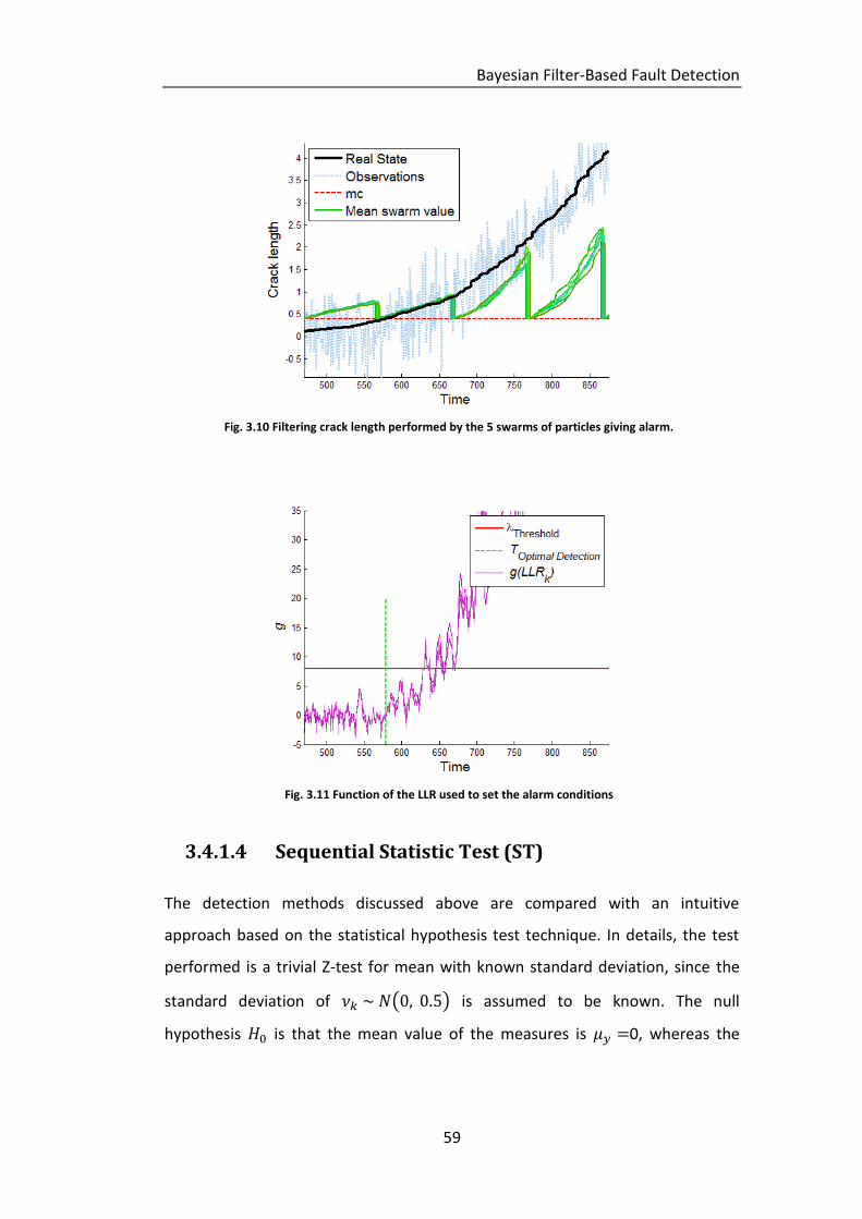
Bayesian Filter-Based Fault Detection
59
Fig. 3.10 Filtering crack length performed by the 5 swarms of particles giving alarm.
Fig. 3.11 Function of the LLR used to set the alarm conditions
3.4.1.4 Sequential Statistic Test (ST)
The detection methods discussed above are compared with an intuitive
approach based on the statistical hypothesis test technique. In details, the test
performed is a trivial Z-test for mean with known standard deviation, since the
standard deviation of is assumed to be known. The null
hypothesis is that the mean value of the measures is 0, whereas the

Bayesian Filter-Based Fault Detection
60
alternative hypothesis is that . This entails that is refused in favor of
when there is the evidence of the crack presence.
To increase the robustness of the method, the alarm is given when is refused
for an established number of consecutive observations. Thus, if the I
type error of each independent test is set to , the null hypothesis is
refused according to a I type error . In this respect, notice
that if is true, then the observations are independent and identically
distributed random variable.
3.4.1.5 Performance Indicators
To assess the performance of the different approaches, 100 cracks have been
simulated, and used for evaluating the following three performance indicators:
Detection Time Delay [51], i.e., ,
where . This is an indicator of
the promptness of the method in detecting the change in the model.
Crack On Noise, i.e.,
which gives an information about
length of the crack upon detection, compared to the amplitude of the
measure uncertainty. Small values of this indicator relate to an accurate
detection.
False Alarms, i.e., the number of alarms given without that a crack has
occurred. It is a wide spread index for the robustness of the method.
Notice that false alarms are of primary importance in condition monitoring,
being the unnecessary stops of a plant for maintenance operation generally
highly expensive. Thus, the ‘work points’ of the parameters of the considered
detection techniques have been set such that the number of false alarms is
around the acceptability level of 5%. This is supposed to be the best initial setting
to allow a comparison between the three method.
Table 3.1 reports the average values of the three performance indicators,
corresponding to the application of the three considered techniques to the 100
simulated crack growth trials. From this table, it emerges that the two filtering

Bayesian Filter-Based Fault Detection
61
methods IMM and MS have better performances than ST, being the mean values
of the corresponding indicators smaller than those of ST. Moreover, although the
performance in detection of IMM seems not much better than the performance
of MS (2 unit of time, only), it must be kept in mind that IMM has a lower
computational cost than MS, since it needs to run particles instead
of particles simultaneously simulated
in the MS approach. Table 3.2 reports the computational time necessary for
filtering the evolution of one simulated crack growth in seconds.
Notice also that the IMM commits less False Alarms than MS, see Table 3.1.
ST IMM MS
DTD 44.3 19.8 22.1
CON 1.295 1.001 1.025
False Alarms 6% 3% 6%
Table 3.1 Detection Time Delay, Crack On Noise and Percentage of false alarms evaluated on a sample of 100 simulated cracks, for the three methods.
IMM MS
Computational Time (sec) 1.7 32
Table 3.2 Computational time for filtering a crack growth according to the two PF method analyzed.
Finally, sensitivity analyses have been performed to evaluate the dependencies
of the performance from the transition probabilities and the variability of the
measurement noise.
In details, the sensitivity of the methods to the transition probability matrix has
been investigated by varying both the extra-diagonal elements of the matrix
within the set , and correspondingly the values on
its diagonal. Table 3.3 shows that the larger the probability of transition, the
poorer the DTD and CON indicators. These results come from the fact that if
transitions from a model to another are too frequent, then crack length is reset
to null too often, thus preventing the particles from swapping to the correct

Bayesian Filter-Based Fault Detection
62
model. This suggest that when setting the transition matrix, both probability of
occurrence and speed of growth of the crack must be taken into account. On the
other side, if the probability of transition is very small, i.e., = 0.005, the
method of augmenting the state space becomes useless, as on average we have
1 out of 100 particles changing the reference model every two steps. This
consideration explains the worsening of the performance corresponding to =
0.005.
Table 3.3 Detection Time Delay, Crack On Noise and Percentage of false alarms evaluated on a sample of 100 simulated cracks, for the three methods.
A sensitivity analysis has been also carried out for the uncertainty in the
measurement error. The three considered performance indicators have been
evaluated according to different values of the standard deviation of the
measurement noise
. This entails that takes
values of different magnitude with respect to the measurement resolution :
when , then the precision in the measurement system is very
low, whereas it is really high when
. In Table 3.4 and Table 3.5
the 90th percentile of every performance indicator is considered as a synthetic
and conservative indicator of the promptness of the detection of the three
methods. In this respect, other parameters to summarize the distribution such as
the mean, the median, etc., would put emphasis on the performance of the
detection methods in the best cases, whereas the 90th encompasses also the
performance of the methods in the worst cases.
From Table 3.4, it emerges that the DTD values of the three methods are similar
for small values of , whereas the IMM method is by far the most accurate
when is comparable with or higher than the measurement resolution .
A12 0.005 0.01 0.05 0.1
DTD 20.1 18.6 25.1 38.6
CON 1.017 0.9963 1.053 1.237
False Alarms 0% 1% 0% 0%

Bayesian Filter-Based Fault Detection
63
That is, when the measurement error is very small, all the methods are capable
of distinguishing the fault condition from the normal behavior. This result is also
confirmed by Table 3.5, even though apparently it seems to confirm the opposite
conclusion. In this respect, is must be considered that the larger CON values in
correspondence of small values of are due to the resolution of the
measurement system which is fixed to =0.4. That is, as long as the real crack
is shorter than , the measurement system cannot observe any variation, thus
no detection can occur until it is long at least . Hence also the optimal value of
CON (the crack is detected exactly when it reaches ) takes large value. For
example, the optimal CON according to =0.0675 is
.
Notice that, the decreasing performances of the method proposed in [12] are
related to its need of a larger window to catch the difference between the two
models. This is confirmed by the ascending values of the 90th percentile of MS,
, for large value of . However, even if is set to its best value (i.e.,
=300), its DTD is still worse than that of IMM (see Fig. 3.12), and also with
higher computational costs (e.g. according to Table 3.2, the computational time
is three times longer, 95 sec / crack). Finally, Table 3.6 reports the percentage
of false alarms for the different values of . This performance indicator is
constant for ST; this is due to the fact that the value of the standard deviation
enters directly the statistical tests, which have the same I type error value .
With respect to both the PF-based methods, the false alarm percentage is not-
null only if the standard deviation takes intermediate values, i.e., when takes
a value similar to . This is due the fact that the smaller , the more similar
are the observations to the real crack length. Thus the reconstruction provide by
the PF is more accurate. On the other side, the larger , the larger the
probability of acquiring observations having small values, i.e., observations which
can avoid particles to grow or which can change the model parameter resetting
the length of the crack associated (only for the IMM). Thus both the methods
become more conservative.

Bayesian Filter-Based Fault Detection
64
Table 3.4 90th
percentiles of the DTD performance indicator for ST, IMM and MS, and for increasing
values of the standard deviation of the measurement noise.
Table 3.5 90th
percentiles of the CON performance indicator for ST, IMM and MS, and for increasing
values of the standard deviation of the measurement noise.
Table 3.6 Percentage of false alarms evaluated for different values of the standard deviation of the measurement noise.
0.0675 0.125 0.25 0.5 1 2 4
ST 4 6 19,2 73,2 155 257 387,3
IMM 3 5 12,6 29 71,6 151,6 248
MS 1 3 10 36 123 275 569,5
0.0675 0.125 0.25 0.5 1 2 4
ST 7,02 3,55 2,01 1,67 1,49 1,42 1,35
IMM 6,88 3,54 1,88 1,11 0,83 0,74 0,68
MS 6,76 3,46 1,85 1,21 1,24 1,59 2,74
0.0675 0.125 0.25 0.5 1 2 4
ST False Alarms 6 6 6 6 6 6 6
IMM False Alarms 0 0 1 3 3 1 0
MS False Alarms 0 4 10 6 0 0 0
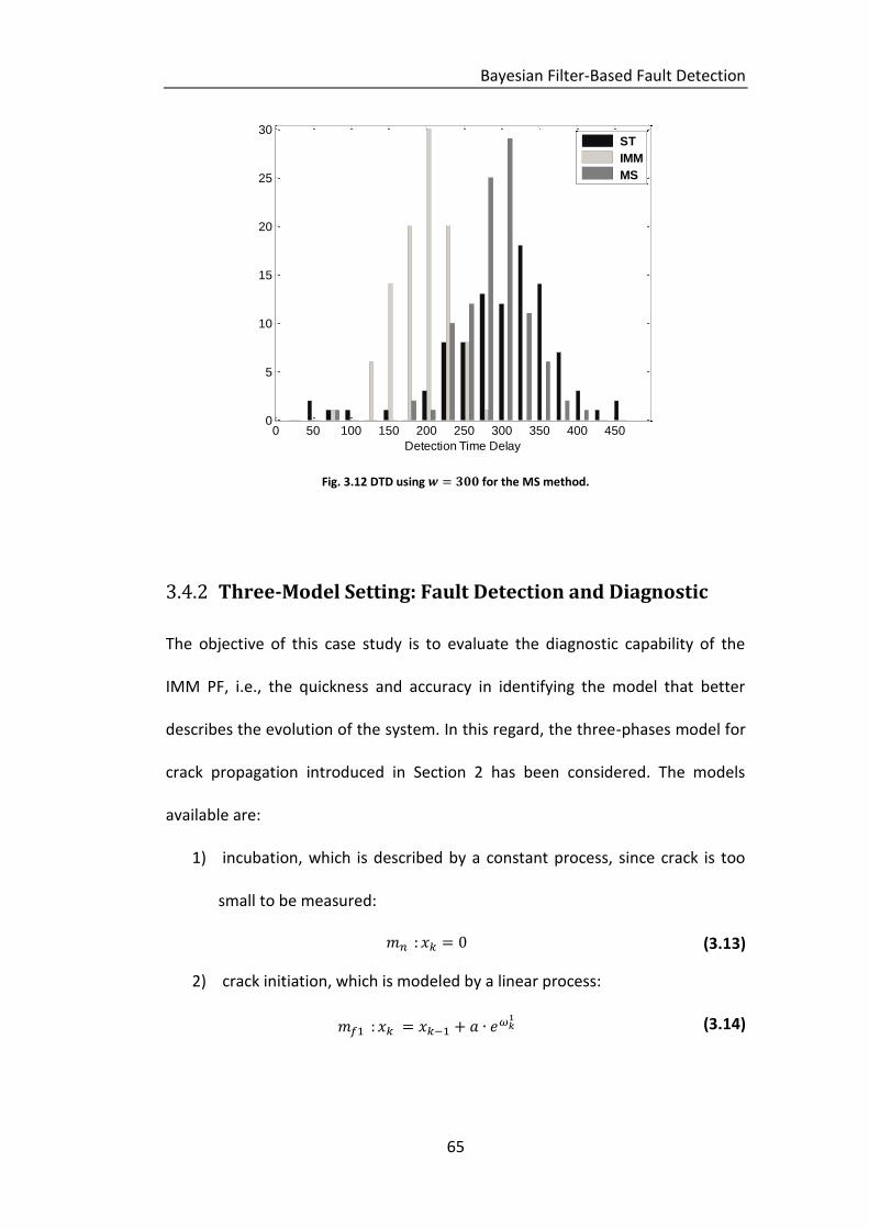
Bayesian Filter-Based Fault Detection
65
Fig. 3.12 DTD using for the MS method.
3.4.2 Three-Model Setting: Fault Detection and Diagnostic
The objective of this case study is to evaluate the diagnostic capability of the
IMM PF, i.e., the quickness and accuracy in identifying the model that better
describes the evolution of the system. In this regard, the three-phases model for
crack propagation introduced in Section 2 has been considered. The models
available are:
1) incubation, which is described by a constant process, since crack is too
small to be measured:
(3.13)
2) crack initiation, which is modeled by a linear process:
(3.14)
0 50 100 150 200 250 300 350 400 4500
5
10
15
20
25
30
Detection Time Delay
ST
IMM
MS

Bayesian Filter-Based Fault Detection
66
where is the speed of growth parameter, and
modes the uncertainty in the speed;
3) crack rapid-propagation, which is again described by the Paris-Erdogan
model:
(3.15)
where the parameter values are the same of the two model system.
The measurement system is that in Eq. (3.11), with the same parameter values.
Notice that the distribution of the noise in the initiating phase is different from
that in the rapid-propagation phase. This gives due account to the fact that the
evolution of an incipient crack is highly influenced by exogenous factors, and
hardly measurable due to its small length. Hence, its uncertainty is expected to
be larger.
Fig. 3.13 reports the simulation of possible crack evolutions, whereas a possible
measure of a crack degradation process is represented in Fig. 3.14. All the
simulated crack growth processes start at units of time, and follow
the initiating linear model in Eq. (3.14) up to units of time, when they
switch to the Paris-Erdogan model in Eq. (3.15). In this respect, notice that the
performance indicators are related to the identification delay time; then, the
choice of setting a fixed swap time does not affect the generality of the results.

Bayesian Filter-Based Fault Detection
67
Fig. 3.13 Simulation of 30 cracks with the same starting time step and same swicth time step to P-E model .
Fig. 3.14 Trajectory of a simulated crack and a respectively possible measurement process (dot line).
Performances have been tested by simulating crack growth
processes, and evaluating the following performance indicators:
Detection Time Delay (DTD), which is the time span between the start of
the initiating phase and its detection.
0 200 400 600 800 1000 12000
2
4
6
8
10
12
14
16
Time
Cra
ck L
en
gth
0 200 400 600 800 1000 1200-2
0
2
4
6
8
10
12
Time
Observation
Real State

Bayesian Filter-Based Fault Detection
68
Transition Time Delay (TTD), which is the time span between the start of
the rapid-propagation phase and its detection.
Percentage of False alarms, which can concern both the two transitions.
On the basis of considerations similar to those of the previous cases study, the
transition probability matrix is set to:
(3.16)
The number of particles is set to as in the previous case study, and the
detection threshold is set to , with a number of
consecutive detections required to give the detection alarm.
Fig. 3.15 shows that the IMM is able to detect the changes in the operational
models on the basis of the marginal posterior probability in Eqs. (3.6) and (3.8),
with good filtering performances, as confirmed by Fig. 3.16. Indeed, in the first
phase (i.e., ) the marginal probability associated to the
incubation model takes by far the highest value; in the second phase (i.e.,
) the probability of the initiating model takes by
far the highest value, whereas in the last phase the value associated to the
rapid-propagation model takes the highest value.

Bayesian Filter-Based Fault Detection
69
Fig. 3.15 Marginal posterior probability for every operating models.
Fig. 3.16 IMM filtering of the real length of the crack.
Notice that the identification of the transition between incubation and initiating
model (i.e., is more accurate than that between the initiating and
the rapid-propagation models (i.e., ), as it emerges from the large
0 200 400 600 800 1000 12000
0.2
0.4
0.6
0.8
1
1.2
1.4
Time
P( k = 0 | Y
k) : NO Crack
P( k = 1 | Y
k) : Linear Model
P( k = 2 | Y
k) : P-E Model
T
0 200 400 600 800 1000 1200-2
0
2
4
6
8
10
12
14
Time
Cra
ck's
Le
ng
th
Observation
Real State
Filtering State

Bayesian Filter-Based Fault Detection
70
time window in which there is high uncertainty in the variable D to be associated
to (i.e. the high overlapping in the time span in Fig. 3.16) . In
this respect, Fig. 3.17 and Fig. 3.18 show that the distribution of the DTD is
centered on a smaller value and presents a sharper shape than that of the
distribution of the TTD. This is due to the smooth transition between the
propagation models in Eqs. (3.14) and (3.15), as confirmed by the percentage of
false alarms reported in Table 3.7, which is smaller in the first transition.
Different choices of and entail different performances.
Intuitively, small values of and make the method sensitive to
possible outliers related to measurement noise, as it is confirmed by the high
percentage of false alarms, see Fig. 3.19. On the other side, large values of
and make the method more conservative, as it is confirmed by
the increased delay in DTD and TTD.
Finally, Table 3.8 and Table 3.9 report the 90th percentile of the DDT and TTD for
increasing values of and , respectively. As expected, the
percentile take value in ascending order according to both increasing value of
and

Bayesian Filter-Based Fault Detection
71
Fig. 3.17 Histogram of the DTD from the incubation model to the initiating model.
Fig. 3.18 Histogram of the TTD from the initiating model to the P-E model.
Transition
False Alarms 2.2% 5%
Table 3.7 Percentage of false alarms evaluated on 500 simulated cracks.
-20 0 20 40 60 80 1000
20
40
60
80
100
120
140
Detection Time Delay mn to m
f1
-20 0 20 40 60 80 100 120 140 1600
10
20
30
40
50
60
70
80
Transition Time Delay mf1
to mf2

Bayesian Filter-Based Fault Detection
72
Fig. 3.19 percentage of false alarms: Left column sensitivity to ; right column sensitivity to .
Table 3.8 90th
percentile of DTD and TTD for ascending values of consecutive detection.
Table 3.9 90th
percentile of DTD and TTD for ascending values of the detection threshold.
3.5 Conclusion
This chapter has investigated the potential of a PF approach based on an
augmented state vector for fault detection and isolation in nonlinear multi-
1 3 5 7 90
10
20
30
40
50
60
70
seqdetection
% F
als
e A
larm
s
DTD
TTD
0.6 0.7 0.8 0.90
2
4
6
8
10
12
T
% F
als
e A
larm
s
DTD
TTD
1 3 5 7 9
17 23 36 67 142,5
75,8 81 99 134,1 187
0.6 0.7 0.8 0.9
30 31 36 50
78 86,5 99 146

Bayesian Filter-Based Fault Detection
73
model smooth degradation processes. By way of a case study concerning the
crack growth degradation process, it has been shown that such approach,
referred to as IMM, is capable of performing an accurate and prompt detection
of the crack occurrence, and provides also a robust estimation of the real length
of the crack. Furthermore, the diagnostic capability of this method has been
confirmed even when the degradation process is modeled evolving among three
phases, with smooth transitions from one phase to another.
The performance of the IMM method have been compared to those of an
already available PF technique of the literature, and of a statistical sequential
test method by way of a two-phase crack degradation process. It has emerged
that the FDI performance of the IMM techniques is better than those of the
other two methods, regarding prompt detection and computational cost..
Moreover, the introduction of the augmented state which explicitly indicates the
process phase, makes the FDI problem much more easily comprehensible.
Indeed, the information provided by the method is the probability that the
monitored component is in a specific degradation phase,.

74
4
Conclusions
In this work, fault detection of industrial components has been considered. Two
novel contributes which aim at an early and accurate identification of the
incipient abnormal condition of the component behavior, have been proposed.
Respectively the former regarding data-driven methods, the latter model-based
methods. With respect to data-driven methods, this work has focused on the
AutoAssociative Kernel Regression (AAKR). In order to obtain more robust signal
reconstructions of the expected values of the monitored signals in normal
conditions, a modification of the traditional AAKR method has been proposed.
The modification is based on a different procedure for the computation of the
similarity between the present and the historical measurements. In particular,
before the computation of the Kernel between the two vectors, which is
performed as in the traditional AAKR method according to a Gaussian RBF
function, the data are projected into a new signal space defined by using a
penalization vector which reduces the contribution of signals affected by
malfunctioning. The procedure is based on the hypothesis that the probability of
occurrence of a fault causing variations on a large number of signals is lower than
that of one causing variations on a small number of signals.
Conclusions
75
The modified AAKR method has been applied to a real case study concerning the
monitoring of 6 highly correlated signals in an industrial plant for energy
production. The possibility of detecting sensor faults has been investigated. The
obtained results have shown that the reconstructions provided by the modified
AAKR are more robust than those obtained by using the traditional AAKR. This
causes a reduction in the time necessary to detect abnormal conditions and in a
more accurate identification of the signals actually affected by the abnormal
conditions.
On the other side, with respect to model-based methods, this work has focused
on a Particle Filtering PF approach based on an augmented state vector where
the augmented state represents the possible behavior of the component. At the
best of the author’s knowledge, this is the first time, that it has been applied for
detection and diagnostic where more than two models are available, the noise in
the model is non-Gaussian and the degradation process is smoothly evolving. By
way of a case study concerning the crack growth degradation process, it has
been shown that such approach, referred to as IMM, is capable of performing an
accurate and prompt detection of the crack occurrence, and provides also a
robust estimation of the real length of the crack. The performances of the IMM
method have been compared to those of an already available PF technique of
the literature, and of a statistical sequential test method by way of a two-phase
crack degradation process. It has emerged that the FDI performances of the IMM
techniques are better than those of the other two methods. Furthermore, the
method has been capable of diagnosing the correct phase degradation even
when the degradation process is modeled as evolving among three phases, with
smooth transitions from one phase to another. Finally, the introduction of the
augmented state which explicitly indicates the process phase, makes the results
of FDI problem easily comprehensible since the information provided by the
method is the probability of being in a specific degradation phase.
To conclude, according to the data-driven method, future works will be devoted
to the demonstration that the whole procedure proposed for the evaluation of

Conclusions
76
the weights, i.e. the pre-processing step and the application of a Gaussian kernel,
is itself a kernel function. The application of the method to additional real case
studies of degradation of components is also foreseen.
On the other side the diagnostic ability of the model-based method provides a
good framework for developing some decision-making criteria. In this respect,
future works will focus on the introduction in the model of a risk function, which
takes into account the costs associated to false alarms and to identification
delays. This could give the opportunity of developing a risk-based FDI.

77
References
[1] Alrowaie F., R.B.Gopaluni n, K.E.Kwok, 2012, “Fault detection and isolation in
stochastic non-linear state-space models using particle filters”, Control
Engineering Practice, vol. 20, 1016–1032.
[2] Arulampalam S., Maskell S., Gordon N., Clapp T., 2002, “A tutorial on
particle filters for on-line nonlinear/non-Gaussian Bayesian tracking”, IEEE
Transaction on Signal Processing, vol. 50, No. 2, pp. 174-188.
[3] Baraldi P., Canesi R., Zio E., Seraoui R., Chevalier R., 2011, “Genetic algorithm-
based wrapper approach for grouping conditional monitoring signals of
nuclear power plant system”, Integrated computer-Aided engineering, vol.
18,pp. 221-234.
[4] Baraldi P., Di Maio F., Pappaglione L., Zio E. and Seraoui R., 2012, “Condition
Monitoring of Power Plant Components During Operational
Transients”,Journal of Risk and Reliability.
[5] Baraldi P., Gola G., Zio E., Roverso D., Hoffman M., 2011, “A randomize model
ensemble approach for reconstructing signals from faulty sensors”, Expert
systems with application, vol 38, No. 8.
[6] Baraldi P., Mangili F., Zio E., 2012, “A Kalman filter-based ensemble
approach with application to turbine creep prognostics”, IEEE Transaction
on Reliability, vol. 61, No. 4, pp. 966-977.
[7] Basseville M., 1988. “Detecting Changes in Signals and System – A survey”,
Automatica, vol. 24, No. 3, pp. 309-326.
[8] Bishop C., 1995, “Neural Networks for Pattern Recognition”, Oxford
University Press, NY, USA.
References
78
[9] Boursier J.M., Desjardins D. and Vaillant F., 1995, “The Influence of the
strain-rate on the stress corrosion cracking of alloy 600 in high temperature
primary water”, Corrosion Science, vol. 37, No. 3, pp. 493-508.
[10] Burges C. J.C., 1998, “A Tutorial on Support Vector Machines for Pattern
Recognition”, Data Mining and Knowledge Discovery, vol. 2., pp. 121-167
[11] Cadini F., Zio E., Avram D., 2009, “Model-based Monte Carlo state
estimation for condition-based component replacement”, Reliability
Engineering and System Safety, vol. 94,pp. 752-758.
[12] Cadini F., Zio E., Giovanni Peloni, 2012, “Particle Filtering for the Detection
of Fault Onset Time in Hybrid Dynamic Systems With Autonomous
Transitions”, IEEE Transaction on reliability, vol. 61, No. 1, pp. 130-139.
[13] Candy J.V., 2009, “Bayesian Signal Processing: Classical, Modern and
Particle Filtering Methods”, IEEE and Wiley, New Jersey.
[14] Castanier B., C.Bérenguer and Grall A., 2003, “A sequential condition-
based repair/replacement policy with non-periodic inspections for a system
subject to continuous wear”, Applied Stochastic Models in Business and
Industry, vol. 19, No 4, pp. 327-347.
[15] Chevalier R., Provost D., and Seraoui R., 2009, “Assessment of Statistical
and Classification Models For Monitoring EDF’s Assets”,Sixth American
Nuclear Society International Topical Meeting on Nuclear Plant
Instrumentation.
[16] Di Maio, F.; Baraldi, P.; Zio, E.; Seraoui, R., 2013, "Fault Detection in
Nuclear Power Plants Components by a Combination of Statistical Methods,"
Reliability, IEEE Transactions on, Accept, not published.
[17] Doucet A. N., Johansen A. M., 2008, “A Tutorial on particle filtering and
smoothing: Fifteen years later”.
[18] Doucet. A., N. De Freitas and N.J. Gordon, 2001, “An introduction to
Sequential Monte Carlo Methods” in SMC in Practice, Springer-Verlag, New
York.

References
79
[19] Dunia R., Qin S.J., Edgar T.F., McAvoy T.J., 1996, “Identification of Faulty
Sensors Using Principal Component Analysis”, AlChE Journal, vol.42, No.10,
pp. 2797-2811.
[20] Feller S., Todorov Y., Jaroszewski D., Chevalier R., 2013, “Taming Anomaly
Detection for Industrial Applications”, AIP Conference Proceedings, vol. 1558,
pp. 2257-2260
[21] Gordon, N. J., Salmond, D. J., and Smith, A. F. M., 1993, “Novel approach
to non-linear/non-Gaussian Bayesian state estimation”, IEE Proceedings–F,
140, 107–113.
[22] Grall, A., Blain, C., Barros, A., Lefebvre, Y., F.Billy, 2007, “Modeling of
Stress Corrorsion Cracking with Periodic Inspection”, Proceeding of the 32nd
ESReDA Seminar, Alghero, Italy Maintenance Modeling and Application,
vol. 1, pp. 253-260.
[23] Guglielmi G., Parisini T., Rossi G., 1995, “Fault Diagnosis And Neural
Networks: A Power Plant Application”, Control Engineering Practice, vol. 3,
No. 5, pp. 601-620.
[24] Harkat M.F., Djelel S., Doghmane N., Benouaret M., 2007, “Sensor Fault
Detection, Isolation and Reconstruction Using Nonlinear Principal Component
Analysis”, International Journal of Automation and Computing, vol. 4, No. 2,
pp. 149-155.
[25] Henk A., Blom P., Bar-shalom Y., 1988, “The interacting multiple model
algorithm for system with Markovian switching coefficients”, IEEE
Transactions on Automatic Control, vol. 33, No. 8.
[26] Hines J. W., Garvey D., 2006, “Development and Application of Fault
Detectability Performance Metrics for Instrument Calibration Verification and
Anomaly Detection”, Journal of Pattern Recognition Research, vol. 1, pp. 2-
15.
[27] Hines J. W., Garvey D., 2007, “Process and Equipment Monitoring
Methodologies Applied to Sensor Calibration Monitoring”, Quality and
Reliability Interantional, vol. 23, No. 1, pp. 123-135.
[28] Hsu C., Chang C., Lin C., 2003, “A Practical Guide to Support Vector
Classification”, Department of Computer Science and Information
Engineering, National Taiwan University, Taipei.

References
80
[29] Jardine A., Lin D., Banjevic D., 2006, “A review on machinery diagnostics
and prognostics implementing condition based maintenance”, Mechanical
Systems and Signal Processing, vol. 20, No. 7, pp. 1483–1510.
[30] Julier, S. J. and Uhlmann, J. K., 1997, “A new extension of the Kalman filter
to nonlinear systems”, SPIE Aerospace Symposium.
[31] Kadirkamanathan V., Li P., 2001, “Particle Filtering based likelihood ration
approach to fault diagnosis in nonlinear stochastic system”, IEEE Transaction
on Systems, Man and Cybernetics – part C: Application and Reviews, vol. 31,
No. 3,pp. 337-343.
[32] Kadirkamanathan V., Li P., 2004, “Fault detection and isolation in non-
linear stochastic systems–A combined adaptive Monte Carlo filtering and
likelihood ratio approach”, International Journal of Systems Science, vol. 77,
No. 12, pp. 1101–1114.
[33] Kadirkamanathan V., Li P.,Jawardand M., Fabri S., 2002, “Particle filtering-
based fault detection in nonlinear stochastic systems”, International Journal
of Systems Science, vol. 33, No. 4, pp. 259–265.
[34] Liu J.S., Chen R., 1998, “Sequential Monte Carlo method for dynamic
system”, Journal of the America Statistic Association, vol. 93, No. 443.
[35] Liu W., Principe J., Haykin S., 2010, “Kernel Adaptive Filtering: A
Comprehensive Introduction”, John Wiley, Hoboken, New Jersey, USA.
[36] Mehra, M. Rago, C. and Seereeram, S., 1998, “Autonomous failure
detection, identification and fault-tolerant estimation with aerospace
applications”, in Proceedings of IEEE Aerospace Conference, Vol. 2, pp.133-
138.
[37] Mehra, M., Seereeram, S., Bayard, D. and Hadaegh, F., 1995, “Adaptive
Kalman filtering, failure detection and identification for spacecraft attitude
estimation”, in Proceedings of the 4th IEEE Conference on Control
Applications, pp.176-181.
[38] Nabeshima K., Suzudo T., Suzuki K., Turcan E., 1998, “Real-time Nuclear
Power Plant Monitoring with Neural Network”, Journal of Nuclear Science
and Technology,vol. 35, No. 2, pp. 93-100.
References
81
[39] Orchard M., Vachtsevanos G., 2009, “A particle-filtering approach for on-
line fault diagnosis and failure prognosis”, Transactions of the Institute of
Measurement and Control, vol. 31,No. ¾, pp. 221–246.
[40] Paris P., Erdogan F., 1963, “A Critical Analysis of Crack Propagation
Laws”, Journal of Basic Engineering, vol. 85, No. 4, pp. 528-533.
[41] Rasmussen C., Williams C., 2006, “Gaussian Processes for Machine
Learning”, MIT Press, Cambridge, MA, USA.
[42] Thrun S., Langford J., Verma V., 2001, “Risk sensitive particle filters”,
Advances in Neural Information Processing Systems, vol. 14.
[43] Venkatasubramanian V., R. Rengaswamy, K. Yin, S. N. Kavuri, 2003, “A
review of process fault detection and diagnosis Part I: Quantitative model-
based methods”, Computers and Chemical Engineering, vol. 27, pp. 293-311.
[44] Venkatasubramanian V., R. Rengaswamy, S. N. Kavuri, 2003, “A review of
process fault detection and diagnosis Part II: Qualitative models and search
strategies”, Computers and Chemical Engineering, vol. 27, pp. 313-326.
[45] Venkatasubramanian V., R. Rengaswamy, S. N. Kavuri, K. Yin, 2003, “A
review of process fault detection and diagnosis Part III: Process history based
methods”, Computers and Chemical Engineering, vol. 27,pp. 327-346.
[46] Wang X., Syrmos V. L., 2008, “Interacting Multiple Particle Filters For Fault
Diagnosis of Non-linear Stochastic Systems”, American Control Conference,
Seattle, USA.
[47] Willsky A.S. et al., 1980, “Dynamic model-based techniques for the
detection of incidents on freeways”, IEEE Trans. Automat. Contr., vol. AC-25.
[48] Worden K., Staszewski W., Hensman J., 2011, “Natural computing for
mechanical systems research: a tutorial overview”, Mechanical Systems and
Signal Processing, vol. 25, No. 1,pp. 4–111.
[49] Zhang B., Sconyers C., Byington C., Patrick R., Orchard M., Vachtsevanos
G., 2008, “Anomaly detection: a robust approach to detection of
unanticipated faults”, International conference on prognostics and health
management.

References
82
[50] Zhang B., Sconyers C., Byington C., Patrick R., Orchard M., Vachtsevanos
G., 2011, “A probabilistic fault detection approach: application to bearing
fault detection”, IEEE transaction on industrial electronics, vol. 58, No. 5.,
2011-2018.
[51] Zio E., 2013, “Diagnostic and Prognostic of Engineering System: Methods
and Techniques”, IGI Global, pp. 333-356.

83
Appendix:
Particle Filtering
Particle Filtering (PF) has roots in the Bayesian framework and roughly speaking
it consists in the approximation of the distribution of interest via a sequence of
empirical distributions. To the best reader comprehension the appendix is
structured as follow: section A.1 Nonlinear Bayesian Filtering presents the
nonlinear bayesian filtering; section A.2 Monte Carlo Perfect Sampling
reports monte carlo perfect sampling; in section A.3 Particle Filtering the
Sequential Monte Carlo (SMC) method a.k.a. Particle Filtering is introduced;
section A.4 Sequential Importance Resampling (SIR) present structure of the
algorithm. An exhaustive dissertation could be found in [2], [13], [17], [18], [21].
A.1 Nonlinear Bayesian Filtering
Nonlinear filtering is defined as the process of estimating the state vector
governed by a nonlinear, non-Gaussian state-space model (A.1), using noisy
observation (A.2). Although a continuous-time estimation procedure can be
performed, usually a discrete-time implementation is used since the streaming
measurements data is sent and received through digital devices in most of the
application regarding fault detection and diagnostic.

Appendix: Particle Filtering PF
84
(A.1)
(A.2)
Within a Bayesian general formulation, filtering consists in the estimation of the
posterior probability density function (pdf) of the current state , based on the
set of received measurements. Since filtering is perform every time that a new
observation arrived, to avoid an increasing computational cost and memory
storage, a recursive strategy is pursued. Mathematically, let be an
unobserved process described by a Markov Chain on described by its initial
distribution and the transition probability . is
defined by the state equation (A.1) and the sequence of independent random
variables . Noisy measurements are observable and assumed to
be conditionally independents given the process , equation (A.2) defines
the pdf where is a sequence of independent random variable.
Let and be, respectively, the state and
the measurements up to time ; typical quantity of interest are: the posterior
distribution , the marginal distribution (a.k.a. filtering
distribution) and the expectations:
(A.3)
for any function integrable with respect to .
A recursive expression of the posterior distribution can be found recurring to the
prediction and update steps. The former
(A.4)
the latter according to the Bayes formula
(A.5)
Where
(A.6)

Appendix: Particle Filtering PF
85
However this results are more conceptual than practical, since only in few cases
the integral, thus the quantities of interest, admit solution in closed-form.
Nevertheless the recursive expression lay the foundation for the Sequential
Monte Carlo method.
A.2 Monte Carlo Perfect Sampling
Given a set of samples
, also named particle, i.i.d. from the pdf of
interest an empirical unbias estimation of the distribution and of
the expectation (A.3) is given by:
(A.7)
(A.8)
Thanks to the strong Law of Large Number (LLN) if the second moment is finite
, then
, thus both
the approximations converge to the respective real value almost surely:
moreover, the central limit theorem is valid. Unfortunately it is usually almost
impossible to sample efficiently from the desired distribution cause it is typically
multivariate, non-standard and known up to a proportionality constant. A
common approach is using Markov Chain Monte Carlo (MCMC) methods,
however due to their iterative structure, they are not suitable for a recursive
estimation problem. To avoid this problem importance sampling is a wide spread
technique that allows to sample from a chosen distribution
provided that weights are added to the particles:

Appendix: Particle Filtering PF
86
(A.9)
(A.10)
Or alternatively by normalizing the weights:
(A.11)
(A.12)
However even in this case a recursive approach is not feasible since every time a
new measurement arrives, all the trajectories of the weights of the particles
must be reevaluated, hence the computational cost increases proportionally to
time.
A.3 Particle Filtering
To overcome the problem a sequential approach is pursue, i.e., only the last step
is updated when a new observation becomes available. Importance function
is chosen such as:
(A.13)
Thus by decomposing the posterior as follow
(A.14)
A recursive formulation for the weights (A.10) is given by:
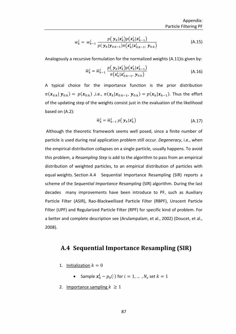
Appendix: Particle Filtering PF
87
(A.15)
Analogously a recursive formulation for the normalized weights (A.11)is given by:
(A.16)
A typical choice for the importance function is the prior distribution
,i.e., . Thus the effort
of the updating step of the weights consist just in the evaluation of the likelihood
based on (A.2):
(A.17)
Although the theoretic framework seems well posed, since a finite number of
particle is used during real application problem still occur. Degeneracy, i.e., when
the empirical distribution collapses on a single particle, usually happens. To avoid
this problem, a Resampling Step is add to the algorithm to pass from an empirical
distribution of weighted particles, to an empirical distribution of particles with
equal weights. Section A.4 Sequential Importance Resampling (SIR) reports a
scheme of the Sequential Importance Resampling (SIR) algorithm. During the last
decades many improvements have been introduce to PF, such as Auxiliary
Particle Filter (ASIR), Rao-Blackwellised Particle Filter (RBPF), Unscent Particle
Filter (UPF) and Regularized Particle Filter (RPF) for specific kind of problem. For
a better and complete description see (Arulampalam, et al., 2002) (Doucet, et al.,
2008).
A.4 Sequential Importance Resampling (SIR)
1. Initialization
Sample for set
2. Importance sampling
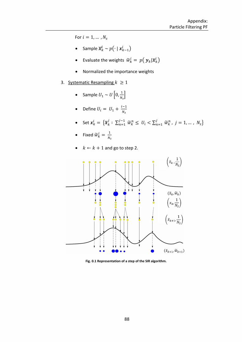
Appendix: Particle Filtering PF
88
For
Sample
Evaluate the weights
Normalized the importance weights
3. Systematic Resampling
Sample
Define
Set
Fixed
and go to step 2.
Fig. 0.1 Representation of a step of the SIR algorithm.