PHYSICAL REVIEW RESEARCH 2, 033110 (2020)

Neural network solutions to differential equations in nonconvex domains:Solving the electric field in the slit-well microfluidic device

Martin Magill ,1,2 Andrew M. Nagel,1 and Hendrick W. de Haan 1,*

1Faculty of Science, University of Ontario Institute of Technology, 2000 Simcoe St N, Oshawa, Ontario, Canada L1H7K42Vector Institute, 661 University Ave Suite 710, Toronto, Ontario, Canada M5G1M1

(Received 29 April 2020; accepted 21 June 2020; published 21 July 2020)

The neural network method of solving differential equations is used to approximate the electric potential andcorresponding electric field in the slit-well microfluidic device. The device’s geometry is nonconvex, makingthis a challenging problem to solve using the neural network method. To validate the method, the neural networksolutions are compared to a reference solution obtained using the finite-element method. Additional metrics arepresented that measure how well the neural networks recover important physical invariants that are not explicitlyenforced during training: spatial symmetries and conservation of electric flux. Finally, as an application-specifictest of validity, neural network electric fields are incorporated into particle simulations. Conveniently, the sameloss functional used to train the neural networks also seems to provide a reliable estimator of the networks’ trueerrors, as measured by any of the metrics considered here. In all metrics, deep neural networks significantlyoutperform shallow neural networks, even when normalized by computational cost. Altogether, the resultssuggest that the neural network method can reliably produce solutions of acceptable accuracy for use insubsequent physical computations, such as particle simulations.

DOI: 10.1103/PhysRevResearch.2.033110

I. INTRODUCTION

Many important phenomena can be modeled effectivelyby partial differential equations (PDEs) with appropriateboundary conditions (BCs). When PDE problems are posedin domains with complicated geometries, they are often toodifficult to be solved analytically, and must instead be ap-proximated numerically. The standard tools for numericallysolving PDE problems in complex geometries are mesh-basedapproaches, such as the finite-element method (FEM) [1]. Inthese methods, the problem domain is decomposed into amesh of smaller subdomains, and the solution is approximatedby a linear combination of simple, local functions.

In this work, we will explore a less common numericalsolution method for PDE problems, which we will refer toas the neural network method (NNM) [2]. In the NNM, thesolution is directly approximated by a neural network (e.g.,Fig. 1), rather than by a linear combination of local basisfunctions. In a process called training, the network parametersare varied until it approximately satisfies the PDE and BCs.

The purpose of this study is to investigate the effectivenessof the NNM on a problem exhibiting a complicated geometry.Specifically, the NNM is used to solve a model of the electricfield in the slit-well microfluidic device, which is an applica-

*Hendrick.deHaan@uoit.ca

Published by the American Physical Society under the terms of theCreative Commons Attribution 4.0 International license. Furtherdistribution of this work must maintain attribution to the author(s)and the published article’s title, journal citation, and DOI.

tion of active research interest [3–6]. The problem domain isnonconvex, and the electric field is discontinuous in the limitof sharp corners. Despite the growing popularity of the NNM,relatively few authors have validated it on problems with suchill-behaved solutions. The rest of this Introduction providesan overview of the NNM, including its previous use to studysystems similar to the slit-well, as well as a review of theslit-well device itself.

A. Neural network method

The neural network method of solving differential equa-tions was first published by Dissanayake and Phan-Thien [2],and belongs to the broader family of techniques known asmethods of weighted residuals [2,7]. Around the same time,Meade Jr. and Fernandez [8] separately demonstrated a variantof the NNM that did not use iterative training, and insteadsolved a system of linear equations for the network weights;it was, however, designed for solving only ordinary differen-tial equations. Later, van Milligen et al. [9] independentlyproposed a method quite similar to the original approachby Dissanayake and Phan-Thien [2], to solve second-orderelliptic PDEs describing plasmas in tokamaks. The NNM wasproposed independently again by Lagaris et al. [10]. Theirmodified methodology embedded the neural network withinan ansatz that was manually constructed to exactly satisfythe boundary conditions; however, this form is challenging toconstruct when the boundary conditions or the domain geom-etry are complicated. Many authors have since contributed tothe development of the NNM, and Yadav et al. [11] publisheda book reviewing much of the early work on the NNM.

2643-1564/2020/2(3)/033110(14) 033110-1 Published by the American Physical Society

MAGILL, NAGEL, AND DE HAAN PHYSICAL REVIEW RESEARCH 2, 033110 (2020)

FIG. 1. Schematic of a fully connected feed-forward neural net-work of depth d and width w mapping coordinates (x, y) to an outputu(x, y). Each node computes a weighted sum of its incoming arrows,and the result (plus a bias) is passed to an activation function. In theNNM, the parameters are optimized to make u(x, y) approximatelysatisfy a target PDE and its BCs.

The NNM has various potential appeals over more com-mon methods like FEM. For instance, the NNM is meshfree, and generally produces uniformly accurate solutionsthroughout the PDE domain [11,12]. Whereas earlier imple-mentations used shallow neural networks (i.e., those havingonly one hidden layer), many authors have recently notedthe significant benefits of using deep architectures [13–26].In particular, it appears that the NNM with deep neural net-works performs remarkably well in high-dimensional prob-lems [13–15,17–19,21–27]. Such high-dimensional PDEs aretypically intractable using FEM and most traditional meth-ods. These suffer from the so-called curse of dimensionality,in which computational cost grows exponentially with thenumber of dimensions. In addition to the above empiricaldemonstrations of the NNM, several theorems have beenpublished stating that the computational cost of the NNMgrows at most polynomially in the number of dimensions forvarious classes of PDEs [28–30].

Nonetheless, the theoretical grounding of the NNM is lessthoroughly developed than those of other techniques. Thereare as of yet few guarantees regarding, e.g., under whatconditions the NNM will converge to the true solution ofa given PDE, at what rate, and to what precision. As such,confidence in the method still relies heavily on empiricaldemonstrations. However, available empirical demonstrationsfocus primarily on problems with relatively well-behavedsolutions [15,16,18,19,21–26,31]. Indeed, Michoski et al. [32]noted this, and conducted an investigation of the NNM appliedto irregular problems exhibiting shocks. This work is analo-gous in this regard, but focuses instead on the nonconvexityof the slit-well domain as the source of irregularity.

B. Slit-well microfluidic device

Microfluidic and nanofluidic devices (MNFDs) are small,synthetically fabricated systems with applications in molec-ular detection and manipulation [5,6,33–35]. One importantuse of MNFDs is to sort mixtures of molecules, includingfree-draining molecules such as DNA that cannot normally beseparated electrophoretically in free solution [6]. For instance,

FIG. 2. A schematic of particles being electrically driven throughthe slit-well device.

the slit-well device proposed by Han and Craighead [3] canbe used for sorting polymers (such as DNA [3,4,36,37]) ornanoparticles [38,39]. The device’s periodic geometry, illus-trated schematically in Fig. 2, consists of parallel channels(called wells) separated by shallower regions (called slits). Anelectric field is applied to drive molecules through the device.

MNFDs such as the slit-well exploit the complexity ofphysical phenomena at the single-molecular scale (often be-low the optical resolution limit) to produce useful and some-times surprising behaviors. This, however, makes them chal-lenging to design and optimize, and renders theoretical andcomputational investigations important to the development ofMNFD technologies. For example, the sorting mechanism inthe slit-well device depends nonlinearly on the magnitude ofthe applied electric field as well as the size and shape of thewells, the slits, and the molecules themselves [6,36–40]. Forsome choices of these parameters, the slit-well sorts molecularmixtures into increasing order of size; for others, however,it sorts them into decreasing order. A rich literature existsexploring these processes, reviewed in part by Dorfman [6]and Langecker et al. [40].

C. NNM with complicated geometries

There are relatively few demonstrations of the NNM onproblems with complicated domain geometries. Specifically,the NNM has mostly been applied to problems posed in rect-angular or circular domains [15,18,19,21–23,25,26]. Of note,Wei et al. [27] used the NNM to solve PDEs in nanobiophysicsthat also arise in MNFDs (i.e., Fokker-Planck for particles andpolymers). However, their work did not consider these prob-lems in MNFD geometries. Even among the demonstrationsof the NNM in more complicated (e.g., nonconvex) domaingeometries, most problems feature boundary conditions thatproduce relatively smooth, well-behaved solutions [16,24,31].Sirignano and Spiliopoulos [17] solved a free-boundary prob-lem based on a financial system, but it is not clear whetherthat PDE exhibits the specific kinds of challenging featuresconsidered in this work.

An exception to the above is given by E et al. [14], whoapplied a variant of the NNM to a Poisson equation in asquare domain with a reentrant needlelike boundary. Thisproblem exhibits the same singular behavior as the slit-wellproblem with sharp corners (see Sec. II A). Their Deep Ritztraining protocol was based on a variational formulation ofPoisson’s equation. However, variational formulations cannotbe obtained for all PDEs [41]. For this reason, we have

033110-2

NEURAL NETWORK SOLUTIONS TO DIFFERENTIAL … PHYSICAL REVIEW RESEARCH 2, 033110 (2020)

opted to study the more general NNM algorithm originallypresented by Dissanayake and Phan-Thien [2].

When Anitescu et al. [42] revisited this needle problemusing the original method of Dissanayake and Phan-Thien [2],they reported poorer convergence than obtained by E et al.[14] with the Deep Ritz method. A similar observation wasmade during this work: reentrant corners significantly impairthe convergence of the standard NNM (Sec. II A). In contrastto this work, the error analyses reported by E et al. [14] andAnitescu et al. [42] did not consider the physical realism ofthe NNM solutions (Sec. I D) nor the accuracy of the NNMsolutions’ gradients. These characteristics of the NNM areimportant for use in various applications, including studies ofMNFDs, and are investigated directly in this work.

D. Physical realism of NNM solutions

Various modifications of the NNM have been proposedto ensure solutions exactly satisfy problem-specific invari-ants that are known a priori, such as boundary conditions[12,16,31], non-negativity [43], Hamiltonian dynamics [44],or special invariants of the Schrödinger equation [45]. How-ever, manually creating formulations of the NNM that explic-itly satisfy specific invariants can be difficult. Furthermore,this approach cannot account for invariants which may beunknown ahead of time. It is natural to question how well theNNM approximates invariant quantities when these are notexplicitly enforced.

In fact, although certain numerical methods can be devisedspecifically to satisfy some conservation laws [e.g., finitevolume methods conserve flux [46], symplectic ordinary dif-ferential equation (ODE) integrators conserve energy [47]),most numerical methods (including standard FEM formula-tions) do not satisfy physical invariants exactly. For instance,Zhang et al. [48] discussed what modifications of the FEMare necessary to render it flux conserving. As part of thiswork, we will investigate how well the NNM satisfies physicalinvariants of the slit-well problem in the absence of anyproblem-specific customization.

II. METHODOLOGY

A. Problem statement

We use the simplest electrostatic model of the electricfield E in the slit-well, namely, the two-dimensional Laplaceequation for the electric potential u. Figure 3 illustrates thegeometry of our model over one periodic subunit of theslit-well device. Uniform Dirichlet boundary conditions wereimposed on the colored segments (specifically, u = ±1 on theright and left, respectively) to model an applied voltage acrossthe system. The gray boundaries correspond to homogeneousNeumann (i.e., insulating) boundary conditions. Throughoutthe interior of the domain (i.e., the yellow area in Fig. 3), thepotential was modeled by Laplace’s equation.

In contrast with other authors, we have rounded the reen-trant corners at the interface of the slits and wells. It canbe shown that near sharp (i.e., nondifferentiable) reentrantcorners, solutions u to Laplace’s equation are not continuouslydifferentiable [49–51]. That is, sharp reentrant corners causesingularities in the electric field E. Because the magnitude of

FIG. 3. A cross-sectional view of the slit-well device illustratingour PDE model of the electric potential in one periodic subunit ofthe device. The reentrant corners follow circular arcs, and the num-bers indicate the lengths of each dotted line. The solution satisfiesLaplace’s equation in the yellow region, Dirichlet conditions on thered and blue boundaries, and homogeneous Neumann conditions onthe gray boundaries.

E near the corners diverges as the curvature goes to zero, theslit-well electric field is ill conditioned, in the sense that smallchanges in the curvature of the corners produce large changesin E.

Although such ill conditioning hinders the performanceof most numerical methods, including FEM [49–51], theypresent a particular challenge for the NNM. The fully con-nected feed-forward neural networks typically used for theNNM are infinitely differentiable functions. However, the truesolution to the slit-well problem with sharp corners exhibitsa discontinuous electric field, so that significant errors seemlikely near the corners. Furthermore, because the neural net-work is a global approximation method, local errors near thecorners can affect performance throughout the domain.

In practice, the training methodology we present here(Sec. II B), when applied to the problem with sharp corners,failed to converge to even a reasonable approximation of thetrue solution. Even in preliminary tests with rounded corners,the convergence rate of the NNM was observed to deteriorateas the curvature of the corners was reduced. Therefore, forthis work, an intermediate curvature (Fig. 3) was selected toproduce a challenging but attainable benchmark for the NNM.

B. NNM implementation

In this section, we describe our implementation of theNNM. It is similar to those of Dissanayake and Phan-Thien[2], van Milligen et al. [9], Berg and Nyström [16], Sirignanoand Spiliopoulos [17], Magill et al. [20], and Wei et al.[27], among others. The true solution u(x) to the PDE wasdirectly approximated by a neural network u(x). This wasaccomplished by training the neural network to minimize theloss functional

L[u] =∫

�

(∇2u)2dA +∫

∂�

(B[u])2ds. (1)

033110-3

MAGILL, NAGEL, AND DE HAAN PHYSICAL REVIEW RESEARCH 2, 033110 (2020)

Here, ∇2u = 0 is the PDE required to hold in the interior ofthe domain � ⊂ R2, and B is a differential operator describingthe boundary conditions Bu = 0 on the boundary ∂� of thedomain (described in Sec. II A and illustrated in Fig. 3). Thus,L[u] quantifies the extent to which the neural network fails tosatisfy the PDE and its boundary conditions.

The parameters of the network were updated iterativelyusing the Adam optimizer, a modified gradient descent al-gorithm [52]. The integrals in L[u] were approximated viathe Monte Carlo method, as described in more detail below.The approximate electric field E and other required deriva-tives were obtained exactly via automatic differentiation. Theweights of the network were initialized by the Glorot method[53]. Computations were done using TENSORFLOW 1.13, andall hyperparameters not discussed here were set to their de-fault values [54].

The Monte Carlo samples xi ∈ � used to estimate the firstterm of L[u] were selected from 100 000 points uniformlydistributed in the bounding rectangle [−Lx, Lx] × [−Ly, Ly],by rejecting those lying outside the domain. Those used toestimate the second term were generated by directly samplingthe boundary with a linear density of 40 points per unitlength. Altogether, this yielded an expected batch size ofroughly 62 000. To reduce the overhead of sampling trainingpoints, batches were reused for 1000 parameter updates beforeresampling.

The testing loss was computed on a set of points sam-pled once at the beginning of training, generated using thesame procedure as the training points. The testing loss wascomputed and recorded every 100 parameter updates. Earlystopping was used to terminate training when the testingloss failed to improve after 100 consecutive tests. The finalnetwork was taken from the epoch at which the testing losswas smallest. This training procedure was conceived to ensurethat networks converged to very stable local minima, in orderto study the behavior of the NNM in the limit of long trainingtime.

The neural networks considered in this study were allfully connected feed-forward networks with tanh activationfunctions (Fig. 1), consisting of d hidden layers of equalwidth w. Specifically, the networks mapped an input vectorx, corresponding to a point in the problem domain, to u givenby

u(x) = fd+1 ◦ fd ◦ · · · ◦ f1(x), (2)

where

f1(x) = tanh (W1x + b1), (3)

fi(x) = tanh[Wi fi−1(x) + bi

], i = 2 . . . d (4)

fd+1(x) = Wd+1 fd (x) + bd+1. (5)

Here, W1 ∈ Rw×2, Wi ∈ Rw×w for i = 2 . . . d , and Wd+1 ∈R1×w are the network’s weight matrices, while bi ∈ Rw fori = 1 . . . d , and bd+1 ∈ R are its biases.

C. FEM implementation

To provide a reliable ground truth against which to com-pare the performance of the NNM, the target PDE was also

solved via the FEM using FENICS [55]. The domain and meshwere constructed using the MSHR package. The resolutionparameter for generate_mesh was set to 200 and the cir-cular reentrant corners were approximated linearly with 100segments each.

In order to obtain an accurate approximation of the electricfield, and not just of the electric potential, the FEM wasapplied to a standard dual-mixed formulation of Laplace’sequation for the electric field and electric potential simulta-neously [55]. In this approach, u and E are approximatedsimultaneously using separate basis functions. Solving for ualone and reconstructing E by differentiation was found toyield poor results.

Convergence tests (not shown) confirmed that the FEMsolution converged in proportion to the square of the meshresolution. The tests suggest that the absolute error in theFEM solution relative to the true solution is on the order ofmachine precision (i.e., 10−16). Note that the FEM solutionwas computed in double precision, whereas the NNM wascomputed in single precision.

III. RESULTS

At its core, the NNM is motivated by the rationale thattraining networks to minimize the loss functional [Eq. (1)]will cause those networks to approximate the correct solution.This section contains investigations into the following relatedquestions:

(1) If a network exhibits a small loss, how close is it tothe true solution? Specifically, is the loss functional a reliableestimator of actual network performance?

(2) If a network is close to the true solution, how well doesit reproduce the physical characteristics of the true solution?Specifically,

(a) to what extent does it exhibit the same spatialsymmetries as the true solution?

(b) to what extent does it conserve electric flux?(3) If a network is close to the true solution, and the corre-

sponding electric field is used to conduct particle simulations,how accurate are subsequent measurements made using thoseparticle simulations?

(4) How does architecture affect these conclusions?All experiments were repeated across four random initial-

izations and multiple network architectures: specifically, allcombinations of depths d = 1, 2, 3, 4, 5, 6 and widths w =10, 25, 50, 75, 100, 150, 200, 250 were examined, as well asnetworks of depth 1 and widths 500 and 1000.

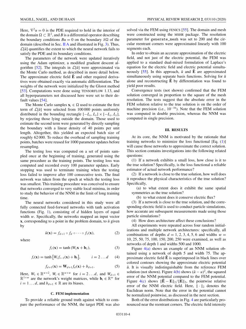
Figure 4(a) shows an example of an NNM solution ob-tained using a network of depth 5 and width 75. The ap-proximate electric field E is superimposed in black lines overcolored contours showing the approximate electric potentialu. It is visually indistinguishable from the reference FEMsolution (not shown). Figure 4(b) shows (u − u)2, the squarederror of the NNM potential compared to the FEM potential.Figure 4(c) shows ‖E − E‖2/‖E‖2, the pointwise relativeerror of the NNM electric field. Here, ‖ · ‖2 denotes theEuclidean norm. Note that the error in the potential cannotbe normalized pointwise, as discussed in the next section.

Both of the error distributions in Fig. 4 are particularly pro-nounced near the reentrant corners. The electric field intensity

033110-4

NEURAL NETWORK SOLUTIONS TO DIFFERENTIAL … PHYSICAL REVIEW RESEARCH 2, 033110 (2020)

FIG. 4. Example NNM solution using 5 hidden layers of width 75. (a) Approximate electric potential (colored contours) and electric field(solid black lines). (b) Squared error of the electric potential. (c) Pointwise relative error in the electric field (note the logarithmic color scale).The errors in plots (b) and (c) are interpolated from values evaluated on the FEM mesh points.

is also very large in these regions (see Fig. 12). In the limit ofsmall curvature, in fact, it is at these corners that the electricfield develops singularities (see Sec. II A). In fact, the peaksin error and electric field intensity both occur precisely wherethe boundary transitions from flat to curved, i.e., where thesecond derivative of the boundary curve is discontinuous.

Additionally, Fig. 4(c) shows pronounced relative errorin the electric field near the corners at the bottom of thewell. These peaks arise because the magnitude of the trueelectric field approaches zero in those corners (see Fig. 12).Since the denominator of ‖E − E‖2/‖E‖2 is very small, evensmall errors in the electric field near those corners manifestas large relative error. The maximum relative error in thedomain � consistently occurred in these bottom-most cornersfor all NNM solutions in the data set. Nonetheless, for manyapplications, errors of this kind are likely to be less importantthan the errors occurring near the reentrant corners, as theyare much smaller in absolute magnitude.

A. Error relative to FEM

The purpose of this section is to investigate the errors ofthe NNM solutions relative to the reference FEM solution,and to what extent the loss functional correlates with theseerrors. The error in an approximate electric potential u will becharacterized by

δu[u] =√√√√⟨

(u − u)2⟩�⟨

u2⟩�

. (6)

Here, 〈·〉� denotes the mean over the domain �. WhereasFig. 4(b) shows the distribution of the squared error in uthroughout the domain, δu[u] corresponds to the root-mean-squared error of u over �, normalized by the root-mean-squared value of the true solution u. Note that one cannotdefine an unambiguous pointwise relative error for u since theelectric potential does not have a physically meaningful zero.The metric δu[u] represents the magnitude of the error in urelative to the magnitude of the true solution u, when both ofthese are measured in the L2 norm for functions.

For the electric field, conversely, a meaningful pointwiserelative error can be defined as ‖E − E‖2/‖E‖2, where boththe numerator and the denominator vary throughout the

domain. The average of this pointwise relative error is denoted

δE[E] =⟨

‖E − E‖2

‖E‖2

⟩�

, (7)

and acts as a global error metric for E. This is precisely themean of error distributions like the one shown in Fig. 4(c).

Figure 5 shows the global error metrics δu[u] and δE[E]for all networks in the data set, plotted against each net-work’s testing loss. The integrals required to compute theerror metrics were approximated via the Monte Carlo method,by sampling the domain interior using the same procedure

FIG. 5. Global error metrics for the NNM solutions relative to thereference FEM solution, shown against testing loss for a variety ofnetwork architectures. (a) The relative error of the electric potentialsδu[u]. (b) The relative error of the electric fields δE[E]. Marker colorindicates the depth of the network, and marker area indicates itswidth.

033110-5

MAGILL, NAGEL, AND DE HAAN PHYSICAL REVIEW RESEARCH 2, 033110 (2020)

described in Sec. II B. Marker color corresponds to networkdepth, and marker size corresponds to network width.

It is clear in Fig. 5 that lower testing losses correlatestrongly with lower values of both δu[u] and δE[E]. This resultconfirms the basic motivation underlying the NNM, namely,that training neural networks to minimize the loss functionalwill cause them to approximate the correct solution. It alsosuggests that, in the absence of theoretical guarantees on theconvergence of the NNM, the testing loss may provide apractical proxy for estimating a solution’s true accuracy.

The data in both Figs. 5(a) and 5(b) partition convenientlyinto two clusters. The upper-right clusters consist of thosenetworks achieving relative errors worse than 1% in both δu[u]and δE[E]. This population contains all of the shallow net-work architectures, suggesting that at least two hidden layersare required to achieve good performance on this problem.Furthermore, as discussed in Sec. III D, shallow networksalways underperform relative to deep networks, even whennormalized by capacity. The narrowest of the deep networkarchitectures also attain relative errors worse than 1%. Thisimplies that even with two hidden layers, networks requiresome minimum capacity (i.e., memory consumption) in orderto achieve good performance on this problem.

The lower-left clusters in Figs. 5(a) and 5(b) contain themajority of the data set, and consist of those networks attain-ing relative errors below 1% in both δu[u] and δE[E]. The bestnetworks achieved relative errors as low as δu[u] ≈ 0.01%and δE[E] ≈ 0.1%. For reference, the example solution shownin Fig. 4 corresponds to a testing loss of L[u] ≈ 9 × 10−6,and error values of δu[u] ≈ 0.2% and δE[E] ≈ 0.08%. Avariety of architecture choices (i.e., depths and widths) pro-duce comparably good performance, suggesting that the NNMcan produce accurate solutions without the need for carefularchitecture tuning. This is explored further in Sec. III D.

B. Physically motivated error metrics

The results in the previous section suggest that the NNMcan reliably produce accurate solutions to the slit-well prob-lem. Furthermore, networks with smaller loss values are closerto the true solution, i.e., they have smaller error values. Fi-nally, the NNM does not appear overly sensitive to the choiceof architecture, given at least two hidden layers and sufficientnetwork width.

The purpose of this section is to investigate whether net-works with small loss and error values also approximatelyreproduce physical characteristics of the true solution. Specifi-cally, we investigate the NNM solutions’ satisfaction of spatialsymmetries and the conservation of electric flux.

1. Deviation from symmetry

The true solution of the target PDE satisfies three spatialsymmetries. First, the true electric potential u is antisymmetricin the horizontal direction about the center of the well, i.e.,

u(x, y) = −u(−x, y), (8)

where (x, y) are the coordinates of a point about the center ofthe well. As a result, the vertical component of the true electric

field E also exhibits this antisymmetry in x, i.e.,

Ey(x, y) = −Ey(−x, y). (9)

Finally, the horizontal component of the electric field is sym-metric about the center of the domain, i.e.,

Ex(x, y) = Ex(−x, y). (10)

The extent to which a network deviates from these symme-tries will be quantified using relative error metrics analogousto those used in the previous section. Specifically, the devia-tion of an approximate electric potential u from symmetry willbe quantified by

Ru[u] =√√√√⟨

(u − u′)2⟩�⟨

u2⟩�

, (11)

where u′(x, y) = −u(−x, y). This is the root-mean-squareddifference between u and its negative reflection, normalizedby the root-mean-squared value of the true potential u. Inanalogy with δu[u], the metric Ru[u] measures the magnitudeof the deviation of u from symmetry relative to the magnitudeof the true solution u (when both are measured in the L2

norm). The deviation of an approximate electric field E fromsymmetry will be quantified by

RE[E] =⟨

‖E − E′‖2

‖E‖2

⟩�

, (12)

where E′ is the transformed electric field

E ′x(x, y) = Ex(−x, y), (13)

E ′y(x, y) = −Ey(−x, y). (14)

In analogy with δE[E], this is the mean pointwise relativedeviation from symmetry of the electric field.

These metrics of deviation from symmetry are closely con-nected to the relative error metrics of Sec. III A. Specifically,the triangle inequality implies that√⟨

(u − u′)2⟩��

√⟨(u − u)2

⟩�

+√⟨

(u − u′)2⟩�. (15)

By definition, the true solution u is invariant under the trans-formation that maps u to u′. Specifically,

u(x, y) − u(x, y) = −u′(−x, y) − ( − u(−x, y)). (16)

By the symmetry of the domain, it follows that√⟨(u − u)2

⟩�

=√⟨

(u − u′)2⟩�. (17)

Combining these results and dividing by√〈u2〉�, it follows

that

Ru[u] � 2δu[u], (18)

that is, the distance from an approximate potential u to itsreflection u′ is, at most, twice the distance from u to thetrue solution u. Very similar reasoning can be applied to anapproximate electric field E to conclude that

RE[E] � 2δE[E]. (19)

033110-6

NEURAL NETWORK SOLUTIONS TO DIFFERENTIAL … PHYSICAL REVIEW RESEARCH 2, 033110 (2020)

FIG. 6. Relative deviation of symmetry for the NNM solutionsnormalized by relative error, shown against testing loss. (a) Deviationof symmetry of the NNM electric potentials Ru[u], divided by therelative error δu[u]. (b) Deviation of symmetry of the NNM electricfields RE[E], divided by the relative error δE[E]. Marker colorindicates the depth of the network, and marker area indicates itswidth. The dotted lines show the upper bounds given by Eqs. (18)and (19).

Thus, solutions with small error values will inevitably benearly symmetric, simply by virtue of being nearly equal to asymmetric function. Furthermore, since it was established inSec. III A that the loss functional provides a reliable estimatorof the error, it follows that the loss also provides a reliableestimator of the deviation from symmetry. It remains to beseen, however, whether or not inequalities (18) and (19)are strict in practice. That is, do neural networks learn thatsymmetry is a desirable feature, or are they only symmetricinsofar as they approximate the true solution?

Figure 6 shows Ru[u]/δu[u] and RE[E]/δE[E] for all net-works in the data set, plotted against each network’s testingloss. As in Fig. 5, the marker sizes correspond to networkwidths, and the colors indicate network depth. The dottedlines correspond to the maximum deviation from symmetrypermitted for a given error value, according to inequalities(18) and (19).

Most of the data in Fig. 6(a) lie nearly on the dotted line:roughly 90% lie above 1.5, and 75% lie above 1.9. This indi-cates that most of the electric potentials approximated via theNNM satisfy the target symmetries only to the smallest degreerequired by virtue of their proximity to the true solution. Thedata in Fig. 6(b), however, lie somewhat farther from thedotted line. Quite a few of the most symmetric electric fieldapproximations have RE[E]/δE[E] ratios below 1, indicating

that they are more similar to their own reflections than theyare to the true solution. It is important to note, however,that the electric field metrics of error and symmetry are nor-malized pointwise by the electric field intensity, whereas theelectric potential metrics are not normalized pointwise. Thisdistinction may account for some of the apparent differencesbetween Figs. 6(a) and 6(b).

Altogether, the results in this section indicate that the NNMsolutions deviate from the symmetries of the true solution byan amount comparable to their error values. Some networksmay produce electric field solutions that are more symmetricthan required given their error values alone, but most networksonly exhibit the minimal degree of symmetry required by thetriangle inequality. As discussed in the Introduction, directlyconstraining the networks to satisfy the symmetries (e.g., bymodifying the network architectures, or by adding additionalterms to the loss functional) would almost certainly improvethe symmetry of the resulting approximations. However, im-plementing such constraints can be expensive for more com-plicated invariants, and some problems may exhibit invariantsthat are unknown a priori. These results illustrate that theNNM can still learn to satisfy invariants approximately, evenwhen they are not explicitly enforced. Furthermore, the lossfunctional may provide a means of empirically estimating theextent to which such invariants are satisfied in practice.

2. Conservation of flux

Another important physical property of the true solution tothe target PDE is the conservation of electric flux. In its strongform, conservation states that the true electric field E must bedivergence free at all points in the domain. This is equivalentto the condition that the true electric potential u must satisfyLaplace’s equation ∇2u = 0 since it can be rewritten as

∇ · (∇u) = ∇ · E = 0. (20)

Thus, one could quantify the deviation from conservation offlux of an approximate field E by computing some error normof ∇ · E. However, since all the derivatives taken in the NNMare exact (obtained via automatic differentiation), ∇ · E isexactly equal to ∇2u. As a result, the first term of the lossfunctional [Eq. (1)] is precisely a measure of how well theNNM satisfies the strong form of the conservation of flux.

Nonetheless, the strong form of conservation is insufficientto fully describe the extent to which the electric field con-serves flux over extended regions of space within the domain.This is better described using the weak form, which statesthat the surface integral of the flux into any closed subset ofthe domain must be zero. Motivated by this, we define thequantity

E (u; ε) = 1

|�ε |∫

�ε

[1

|Bε |∫

∂B(x;ε)Ends

]2

dA. (21)

Here, B(x; ε) is a ball of radius ε centered at a point x inthe domain, ∂B(x; ε) denotes its boundary, and En denotesthe outward normal component of the electric field into itssurface. The outer integral is taken over �ε , by which wedenote the set of all points in the domain that are at least adistance ε from the boundary. The factors |�ε | and |Bε | are theareas of �ε and B(x; ε), respectively. In other words, E (u; ε) is

033110-7

MAGILL, NAGEL, AND DE HAAN PHYSICAL REVIEW RESEARCH 2, 033110 (2020)

FIG. 7. The flux error metric E (u; ε) plotted as a function ofthe ball radius ε for three NNM solutions as well as the referenceFEM solution. The legend entries for the NNM solutions indicate thearchitecture (d,w) for each case. The leftmost points show E (u; 0),and the rightmost show E (u; ∂�). The dotted vertical line labeledLmesh indicates the mean length scale of the FEM mesh.

the mean-square norm of the flux into all balls of radius ε thatare entirely contained within �, divided by the area of thoseballs. Because this definition of E (u; ε) is mesh agnostic, itcan also be computed directly for a FEM solution. Numericalcalculations of E (u; ε) and related metrics in this section aresomewhat technical, and details are relegated to Appendix B.

Figure 7 shows E (u; ε) computed for a sample of NNMsolutions (colored lines) as well as for the reference FEMsolution (black line). The architectures, losses, and relativeerrors of the three networks shown in Fig. 7 are listed inTable. I. The shape of E (u; ε) measured for the NNM so-lutions in Fig. 7 is representative of what was measured onseveral other NNM solutions (not included). In particular,E (u; ε) was consistently observed to decrease monotonicallywith increasing ε. In Fig. 7, the network with architecture(d,w) = (2, 25) achieved relatively mediocre performance.The (1,200) network performed fairly poorly overall, but wasstill among the best performing shallow networks in the dataset. As expected, the best of the three networks accordingto testing loss and the relative error metrics, (4,150), alsoperformed best in terms of conservation of flux. Similarly,(2,25) outperformed (1,200). We emphasize that the (2,25)network outperforms the (1,200) network in all metrics, de-spite having slightly smaller capacity. This is reflective of thedisproportionately poor performance of shallow architecturesnoted in Secs. III A and III D.

TABLE I. Summary of the NNM solutions selected for the con-servation of flux and particle simulations tests. Columns shown thedepth, width, capacity, testing loss, and relative error of the electricpotential and electric field, for each network.

d w Capacity L[u] δu[u] δE[E]

1 200 801 3 × 10−3 16% 7.4%2 25 751 2 × 10−4 1.7% 0.8%4 150 68551 6 × 10−6 0.02% 0.08%

The behavior of E (u; ε) for the FEM solution differs fromthat of the NNM solutions in some important ways. Whereas,for all three NNM solutions, E (u; ε) is roughly constantbelow ε ≈ 10−1, for the FEM solution E (u; ε) continues toincrease with decreasing ε until at least ε ≈ 10−4. As a result,although the FEM solution achieves better E (u; ε) than allNNM solutions at long length scales, the converse is trueat sufficiently small length scales. The best NNM solutionin Fig. 7, (4,150), exhibits comparable conservation of fluxto the FEM solution at length scales near the mean FEMmesh size Lmesh = √|�|/N , where N is the number of meshelements. At length scales below Lmesh, the (4,150) networkconserves flux more accurately than the FEM solution. Eventhe worst of the three NNM solutions shown in Fig. 7 performscomparably to the FEM solution in conservation of flux atlength scales below ε ≈ 10−3. The relative stability of theNNM at small length scales may be attributable to its mesh-free nature, and is an appealing feature for subsequent use inparticle simulations. Finally, we recall (see Sec. II C) that theFEM solution was computed in double precision, and suggestthat the single precision used for the NNM solutions may be alimiting factor to their performance at large length scales.

For small choices of ε, E (u; ε) converges to a measure ofthe strong form of conservation of flux. By the divergencetheorem, for a continuously differentiable field E, the fluxerror metric E (u; ε) can be rewritten as

E (u; ε) = 1

|�ε |∫

�ε

[1

|Bε |∫

B(x;ε)∇ · E dA′

]2

dA (22)

= mean�ε

[(meanB(x;ε)

(∇ · E)

)2]. (23)

In the remainder of this section, angle brackets 〈·〉S will beused to denote means over any set S. From Eq. (22), it is easyto deduce the limit of E (u; ε) as ε → 0, which will be denotedE (u; 0). Since �ε → � and the mean over B(x; ε) approachesthe identity operator, it follows that

E (u; 0) = 〈(∇ · E)2〉� = 〈(∇2u)2〉�. (24)

The leftmost points in Fig. 7 illustrate E (u; 0) for each ofthe solutions. For the NNM solutions, E (u; ε) converges toE (u; 0) as ε → 0, as expected. This is not the case for theFEM solution, for which E (u; ε) exceeds E (u; 0) for small ε.However, this is not a contradiction, as Eq. (24) was derivedby assuming continuous differentiability.

Equation (24) is precisely the mean of the square de-viation of u from the strong form of conservation of flux.For NNM solutions, E (u; 0) is equal to the first term of theloss functional [Eq. (1)] divided by |�|, and is thereforebounded above by the loss. Given that E (u; ε) was observedto decrease monotonically with ε, this suggests that, as for therelative errors and symmetry errors, the loss provides a usefulestimator of the error in conservation of flux over any lengthscale.

However, as ε increases, the metric E (u; ε) becomes in-creasingly biased because the center of the balls B(x; ε)cannot be placed within a distance ε of the boundaries of thedomain. At moderate values of ε, this means that errors influx conservation in the interior of the domain are weighted

033110-8

NEURAL NETWORK SOLUTIONS TO DIFFERENTIAL … PHYSICAL REVIEW RESEARCH 2, 033110 (2020)

FIG. 8. Error in global flux conservation for all NNM solutionsas a function of each network’s testing loss. Marker color indicatesthe depth of the network, and marker area indicates its width. Thedotted line indicates the corresponding error in the FEM solution.

more heavily than those near the boundaries of the domain.Eventually, when ε > 0.6, the balls are too large to fit insidethe slits of the device, so that only errors inside the wellcontribute to E (u; ε). For this reason, the data in Fig. 7 areonly computed for ε values sufficiently below 0.6 that thisbias is deemed acceptably small. This biased behavior ofE (u; ε) arises because the inner integral in Eq. (22) is basedon circle-shaped test sets. A more meaningful metric of fluxconservation over very long length scales can be obtained byreplacing B(x; ε) with ∂� in Eq. (22). This global flux errorwill be denoted E (u; ∂�), and satisfies

E (u; ∂�) =[ |∂�|

|�| 〈En〉∂�

]2

= [〈∇2u〉�]2. (25)

Thus, E (u; ∂�) is directly connected to 〈En〉∂�, the net fluxthrough ∂�, which is zero for the true solution. Note thatthe second equality in Eq. (25) follows from the divergencetheorem, so it applies to the NNM solutions but not the FEMsolution. Together with the second equality of Eq. (24), thismeans

E (u; 0) − E (u; ∂�) =⟨(∇2u

)2⟩�

− [⟨∇2u⟩�

]2, (26)

which is the variance of ∇2u over �. This is always non-negative, so it follows that

E (u; 0) � E (u; ∂�), (27)

for any u satisfying the second inequalities in both Eqs. (24)and (25).

The rightmost points in Fig. 7 illustrate E (u; ∂�) for eachof the four solutions. Figure 8 shows E (u; ∂�) for all NNMsolutions versus each network’s testing loss; the dotted lineindicates the value for the FEM solution. It is immediatelyevident that E (u; ∂�) relates to testing loss in a similar wayas do the relative error metrics (Fig. 5). As was the case forthe other metrics, E (u; ∂�) decreases with decreasing testingloss, suggesting that testing loss is a useful estimator of globalflux error. Indeed, this is inevitable in the limit of small losssince E (u; ∂�) is bounded above by E (u; 0), which is in turnbounded above by the loss. It also appears that the data inFig. 8 are divided into the same two clusters as the data in

Fig. 5, with the shallow architectures performing worse thannearly all deep architectures.

Somewhat surprisingly, the best of the NNM solutionsappear to conserve flux globally to nearly the same degreeas the reference FEM solution, despite being computed insingle (rather than double) precision. Indeed, one networkwith architecture (4,200) appears to slightly outperform theFEM solution in this respect. However, it is important to notethat E (u; ε) for this (4,200) network (not shown) exhibitsessentially the same behavior as that of the (4,150) networkanalyzed in Fig. 7. In other words, although that particularnetwork performs very well at global flux conservation, FEMdoes a significantly better job at conserving flux over interme-diate length scales. This suggests that, for the NNM solutions,the error in conservation of flux is heterogeneously distributedthroughout the domain, which is consistent with the previousobservation that error in the NNM solutions is significantlylarger near the reentrant corners.

In summary, the metric E (u; ε) provides a mesh-agnosticmeasure of how well an NNM solution conserves flux over alength scale ε. As ε → 0, the limit satisfies Eq. (24), and isbounded above by the loss. Empirically, E (u; ε) is observedto decrease monotonically with ε, so that the loss providesa useful estimator of the error in flux conservation overintermediate length scales, too. Alas, when ε is large relativeto other length scales in the domain, E (u; ε) is a biased metric,as it places less weight on flux lost near the boundaries of thedomain. However, a related measure of global conservationof flux over the entire domain is given by Eq. (25), which isnot biased. This measure, too, is bounded above by the loss.Altogether, the NNM seems capable of reliably producingsolutions that conserve flux to an acceptable level of accuracywithout the need to explicitly enforce this physical invariantduring training. In particular, some of the NNM solutionsconserve flux globally roughly as well as the FEM solution.Furthermore, even relatively mediocre NNM solutions con-serve flux better than the FEM solution over sufficiently smalllength scales.

C. Application to particle simulations

Section III A looked directly at error between NNM andFEM, and Sec. III B looked at error metrics motivated byphysical invariants. Both suggested that the testing loss pro-vides a reliable estimator of the true performance of thenetwork solutions, and that (with appropriate network archi-tectures) the NNM consistently finds solutions with seeminglysmall error values. However, the question of what error valuesare acceptable is subjective, and often depends on the intendedapplication of the numerical solutions. For this reason, thissection will consider the performance of the NNM solutionswhen used as the driving force fields in particle simulations ofBrownian motion in the slit-well device (implemented in theC programming language). The simulation scenario is quitesimilar to those investigated by [38,39].

Simulations of N = 100 000 particles in the slit-well do-main were initialized with all the particles located in themiddle of the same well. The particle positions xi evolved

033110-9

MAGILL, NAGEL, AND DE HAAN PHYSICAL REVIEW RESEARCH 2, 033110 (2020)

according to the discretized Brownian equation

�xi

�t=

√2D

�tR(t ) + q

γE, (28)

where the time step was set to �t = 10−4, the diffusioncoefficient to D = 1, and the friction coefficient to γ = 1.The particle charge q was varied from 1 to 10. The termR(t ) is a random driving force, representing thermal motionof an implicit solvent, and was sampled via the Box-Mullertransform from an independent standard Gaussian distributionfor each particle at each time step.

The driving electric field E was obtained from either thereference FEM solution or from one of the NNM solutions.The electric fields were discretized onto a uniform squaremesh overlain on [−Lx, Lx] × [−Ly, Ly], the smallest bound-ing box containing � (see Sec. II B). The side lengths of themesh elements were set to 0.01. The field experienced bya particle at a given position was approximated by nearest-neighbor interpolation to the mesh. We leave more sophis-ticated coupling between the particle simulations and theelectric fields to future work.

Particles experienced periodic boundary conditions acrossthe left and right sides of the periodic subunit illustratedin Fig. 3, and the boundaries that were insulating in theelectric field problem were treated as reflective in the particlesimulations. The number of times each particle crossed the do-main was tracked, so as to measure its absolute displacementfrom the original position. After tmax = 106 time steps, themean horizontal displacement of the particles from the initialposition 〈x〉 was divided by tmax to obtain an estimate 〈vx〉 ofthe average particle velocity. This average velocity was thendivided by particle charge to estimate the effective particlemobility μ = 〈vx〉/q. The statistical error on this mobilitymeasurement was estimated as s = (σvx /q)/

√N , where σvx is

the standard deviation of the particle velocities.These mobility measurements are shown in Fig. 9(a) for

simulations conducted with the same four electric fields in-vestigated in Sec. III B 2: that of the reference FEM solution,and that of the three NNM solutions summarized in Table I.The simulations using the FEM field were conducted twicewith different random seeds, shown as the two black linesin Fig. 9(a). The difference between these two sets of mea-surements provides a means of distinguishing the errors intro-duced by the electric fields from simple statistical fluctuationson the mobility measurements. In Fig. 9(a), the measurementsof μ made using the networks of architectures (2,25) and(4,150) appear fairly similar to those made using the FEMfield. Conversely, the measurements using the (1,200) archi-tecture are quite easily distinguished from the FEM data. Allsimulations recovered effective mobilities that varied withq, induced in the otherwise free-draining particles by theirinteractions with the slit-well geometry.

The relative error between two mobility measurements μ1

and μ2 was quantified as

μ1 − μ2

μ2. (29)

The colored lines in Fig. 9(b) show the relative errors ofthe NNM-based mobility measurements in Fig. 9(a) versus

FIG. 9. (a) Lines show the mobility measurements μ made usingfour different electric field solutions. The two black lines correspondto separate simulations made using the same reference FEM field.The error bars indicate the estimated statistical error of mobility s.(b) The colored lines show the relative errors between the NNM-based measurements and the first set of FEM-based results. The blackline shows the relative errors between the two sets of FEM-basedmeasurements. The error bars are obtained from the data in (a) viastandard rules for propagation of uncertainty.

the first set of FEM-based measurements. The black linecorresponds to the relative errors between the two sets ofFEM-based measurements. Error bars were estimated viastandard rules for propagation of error.

Unsurprisingly, the errors of the (1,200) architecture aresignificantly larger than those of the other two architectures,and show a clear bias toward underestimating the mobility.Nonetheless, even this crude solution produces errors smallerin magnitude than 5% of the actual mobility. This suggeststhat the current particle simulations are relatively insensitiveto moderate inaccuracies in the driving electric field.

The relative errors of both the (2,25) and (4,150) archi-tectures are comparable to the relative errors between thetwo sets of FEM-based measurements, and lie below 1% forall values of q. However, the relative errors for the (2,25)architecture are negative for all q above 2, whereas the rel-ative errors of the (4,150) architecture are roughly evenlydistributed about 0. This suggests that the (2,25) architectureintroduces a small but detectable systematic bias into themobility measurements. Conversely, the errors of the better(4,150) architecture are comparable to statistical fluctuations,despite the relatively large number of simulated particles,N = 100 000. These results confirm that the best of the NNMsolutions presented in this work are sufficiently accurate for

033110-10

NEURAL NETWORK SOLUTIONS TO DIFFERENTIAL … PHYSICAL REVIEW RESEARCH 2, 033110 (2020)

FIG. 10. Testing loss versus network capacity, colored by net-work depths. The error bars show maxima and minima over fourrandom seeds, and the lines indicate mean performance. The dottedlines at capacities of 5 × 103 and 5 × 104 roughly delineate the threeregimes discussed in the text.

use in particle simulation applications. Moreover, the relativeperformance of the three architectures is consistent with theirvalues of L[u], δu[u], and δE[E] (Table I).

In Fig. 9, the network with architecture (2,25) significantlyoutperforms that with architecture (1,200), despite havingslightly smaller capacity, reemphasizing the advantages ofdeep architectures over shallow ones. Conversely, the muchlarger (4,150) architecture only achieves moderate improve-ments over the (2,25) architecture, reflecting the diminishingreturns associated with increasing network capacity. Thesesubtle impacts of architecture are investigated more closelyin Sec. III D.

D. Effect of network architecture

The previous sections have demonstrated that the testingloss is a useful estimator of several independent error metrics.Specifically, the loss functional appears to reliably estimatethe error relative to the reference FEM solution; the deviationfrom symmetry; the deviation from conservation of flux; andthe error introduced into subsequent mobility measurements.Thus, the loss is a useful single metric of performance viawhich to compare different NNM architectures.

In Fig. 10, the testing loss is plotted against the totalnetwork capacity. Here, network capacity is measured as thetotal number of parameters in the network, given in terms ofthe width w and depth d by

(2 + 1)w + (d − 1)(w + 1)w + (w + 1) (30)

since the networks have two inputs and one output. The col-ored lines in Fig. 10 correspond to different network depths,so that the various capacities within each line identify the net-work widths. The error bars show maxima and minima over allrandom seeds, whereas the lines indicate mean performance.

The data in Fig. 10 show that, for network capacitiesbelow 5 × 103, increasing capacity improves testing loss forany choice of depth. This suggests that, for those networks,insufficient capacity is a primary bottleneck toward repre-senting more accurate approximations of the true solution. In

particular, for the networks with two hidden layers, increasingthe capacity improves the loss by nearly two orders of mag-nitude. Furthermore, in this low-capacity regime, increasingdepth improves performance for a given capacity. In otherwords, when insufficient network capacity is the primarybarrier to improved performance, deeper networks make moreefficient use of that limited resource. Indeed, this is consistentwith the effects of architecture observed in Figs. 5, 7, 8,and 9. Specifically, shallow networks perform particularlypoorly in all metrics throughout this work, even compared tonetworks with comparable capacity and as few as two hiddenlayers.

For deep networks with moderately large capacities (5 ×103 to 5 × 104), testing loss is essentially independent ofnetwork architecture (i.e., independent of both depth andcapacity/width). This suggests that insufficient network ca-pacity is no longer a primary bottleneck to improving solutionaccuracy. The investigation by [20] suggested that the internalrepresentations learned by networks in the NNM becomeessentially independent of width above some critical size, soit is not surprising that loss similarly becomes independent ofwidth. However, it is noteworthy that this limiting loss valueis also independent of network depth (among those with twoor more hidden layers).

For networks with capacities of 5 × 104 or above, testingloss begins to increase with further increases in capacity.Figure 5 illustrates that these same networks sometimes ex-hibit relative errors nearly as high as some shallow networks,despite having two orders of magnitude more capacity. Theirpoor performance can be understood in terms of the difficul-ties commonly encountered in training very deep, wide neuralnetworks. For instance, Berg and Nyström [16] noted similarloss in performance when training networks with five or morehidden layers, and attributed this to vanishing gradients. Re-finements in the network architectures and training algorithmscan be expected to alleviate this phenomenon.

Note that the behavior of these networks with very largecapacities cannot be described in terms of overfitting, anotherproblem commonly encountered by networks with exces-sively large capacities. Overfitting is typically defined as asignificant gap between the training and testing losses ofnetworks. In the NNM, however, the testing and training setsare drawn from identical distributions. In the implementationused here, in particular, the training set is redrawn regularlythroughout training, so that it is fundamentally impossiblefor the network to be overfitting to a specific set of trainingsamples.

Finally, Fig. 11 shows the total training time of the NNMsolutions against testing loss. The same two populationsidentified in Figs. 5 and 8 are evident again in Fig. 11. Thecluster on the right contains all the shallow networks as wellas the narrowest of the deep ones. The cluster on the leftconsists of those networks that attained better than 1% errorrelative to FEM (Fig. 5). Within each cluster, testing loss andtraining time are loosely correlated. For all networks, trainingtime was on the order of hours. However, it is important tonote that the implementation in this work was not concernedwith optimizing the computational efficiency of the NNM, butrather with ensuring that the training process was thoroughlyconverged (Sec. II B).

033110-11

MAGILL, NAGEL, AND DE HAAN PHYSICAL REVIEW RESEARCH 2, 033110 (2020)

FIG. 11. Total training time and final testing loss of the NNMsolutions. Marker color indicates the depth of the network, andmarker area indicates its width.

Once again, the networks in the right cluster performdisproportionately poorly, even though many of them havecapacities comparable to some of those in the left cluster(Fig. 10). Thus, not only do the networks in the left clusterachieve better accuracies (as measured by testing loss orany of the various error metrics in this paper), but they alsofinish training far more rapidly. Further, this conclusion is trueeven between networks of equal capacity. These observationsdemonstrate many benefits of using deeper architectures in theNNM, and several disadvantages of using shallow architec-tures.

IV. CONCLUSIONS

This work investigated the performance of the neural net-work method (NNM) when used to solve the electric potentialand field in the slit-well device. This problem features a non-convex geometry, which makes it particularly challenging tosolve with the NNM. Performance was quantified in multiplemetrics, and compared against a reference FEM solution.

The best network architectures studied here reliablyachieved relative errors below 0.1% in both the potential andthe field. NNM solutions also recovered spatial symmetriesof the true solution to roughly the same extent that theyapproximated the true solution. Regarding conservation offlux, the NNM solutions performed comparably to the ref-erence FEM solution. Finally, particle simulations conductedusing the NNM electric fields yielded mobility measurementsconsistent with those based on the FEM electric field. Ineach of these metrics, the testing loss was found to providea useful estimator of the networks’ true performance. Thatis, networks with smaller losses were found to be closerto the true solution; to more closely approximate the targetsymmetries; to conserve flux more accurately; and to producebetter particle simulations.

These empirical investigations uncovered several valuableinsights for practical use of the NNM. Accurate solutions tophysical problems can be obtained even without explicitlyenforcing known physical invariants of the true problem. Theimportance of architecture was reemphasized: deep archi-tectures consistently outperformed shallow ones, convergingto better solutions in less time and using fewer degrees of

FIG. 12. Electric field intensity of the FEM solution, shown on(a) linear and (b) logarithmic color scales.

freedom. Finally, the testing loss may provide a practicalmeans of gauging a solution’s accuracy, even when the groundtruth is unknown and convergence is not theoretically guaran-teed.

In summary, this work demonstrates that the NNM cansuccessfully solve a problem that is ill conditioned due to thenonconvexity of its domain. The NNM solutions were foundto be particularly appropriate for use in subsequent particlesimulations. This suggests that it could be a useful tool for thestudy of microfluidic and nanofluidic devices (MNFDs) andother biophysical systems. Moreover, differential equationsin domains with complicated geometries arise throughoutphysics and other fields. These results support the feasibilityof using the NNM to solve this fundamental and ubiquitousclass of problems.

ACKNOWLEDGMENT

H.W.d.H. gratefully acknowledges funding from the Natu-ral Sciences and Engineering Research Council (NSERC) inthe form of Discovery Grant No. 2014-06091.

APPENDIX A: ADDITIONAL PLOTS OF THEELECTRIC FIELD SOLUTION

Figure 12 shows the FEM electric field intensity through-out the domain, in both linear and logarithmic color scales.In particular, Fig. 12 illustrates that the peak field intensityoccurs near the reentrant corners, with a magnitude of about

033110-12

NEURAL NETWORK SOLUTIONS TO DIFFERENTIAL … PHYSICAL REVIEW RESEARCH 2, 033110 (2020)

0.36. In the bottom corners of the well, the field intensity isover four orders of magnitude weaker. These features con-tribute to the difficulty of applying the NNM to the slit-wellelectric field problem since the standard loss functional usedduring training places equal weight on all regions of � and∂�. The regions of very intense electric field near the reentrantcorners, specifically, seem to be most difficult to resolve forthe NNM, as seen in the error maps shown in Fig. 4.

APPENDIX B: DETAILS OF FLUX LOSS CALCULATIONS

This Appendix contains descriptions of how the metricsshown in Figs. 7 and 8 were computed. For Fig. 7, the integralsin Eq. (21) were computed by sampling 10 000 uniformlyspaced points on ∂B(x; ε) for each choice of the center x.Candidate samples for the centers were generated according

to the same procedure described in Sec. II B, but with 10 timeshigher sample density, and all points within a distance ε of ∂�

were rejected.The leftmost points in Fig. 7 correspond to Eq. (24). For

the NNM solutions, these were computed by Monte Carlointegration over � using 10 times higher sampling densitythan in Sec. II B. The rightmost points in Fig. 7 correspondto Eq. (25). These were not computed using a Monte Carlointegration approach. Because 〈En〉∂� is a small number com-puted by summing many positive and negative terms, it isvulnerable to catastrophic cancellation. For this reason, it wascomputed using a uniform mesh of points along ∂�, sampledwith 100 times higher density than in Sec. II B. For the FEMsolution, the integrals required for Eqs. (24) and (25) wereboth computed in FENICS using Gaussian quadrature via theassemble command.

[1] R. D. Cook, M. E. Plesha, D. S. Malkus, and R. J. Witt,Concepts and Applications of Finite Element Analysis (Wiley,Hoboken, NJ, 2007).

[2] M. W. M. G. Dissanayake and N. Phan-Thien, Neural-network-based approximations for solving partial differential equations,Commun. Numer. Methods Eng. 10, 195 (1994).

[3] J. Han and H. G. Craighead, Entropic trapping and sievingof long DNA molecules in a nanofluidic channel, J. Vac. Sci.Technol. A 17, 2142 (1999).

[4] J. Han and H. G. Craighead, Separation of long DNA moleculesin a microfabricated entropic trap array, Science 288, 1026(2000).

[5] S. L. Levy and H. G. Craighead, DNA manipulation, sorting,and mapping in nanofluidic systems, Chem. Soc. Rev. 39, 1133(2010).

[6] K. D. Dorfman, DNA electrophoresis in microfabricated de-vices, Rev. Mod. Phys. 82, 2903 (2010).

[7] A. J. Meade Jr. and A. A. Fernandez, The numerical solutionof linear ordinary differential equations by feedforward neuralnetworks, Math. Comput. Modell. 19, 1 (1994).

[8] A. J. Meade Jr. and A. A. Fernandez, Solution of nonlinearordinary differential equations by feedforward neural networks,Math. Comput. Modell. 20, 19 (1994).

[9] B. Ph. van Milligen, V. Tribaldos, and J. A. Jiménez, NeuralNetwork Differential Equation and Plasma Equilibrium Solver,Phys. Rev. Lett. 75, 3594 (1995).

[10] I. E. Lagaris, A. Likas, and D. I. Fotiadis, Artificial neuralnetworks for solving ordinary and partial differential equations,IEEE Trans. Neural Networks 9, 987 (1998).

[11] N. Yadav, A. Yadav, and M. Kumar, An Introduction to NeuralNetwork Methods for Differential Equations (Springer, Berlin,2015).

[12] I. E. Lagaris, A. Likas, and D. I. Fotiadis, Artificial neural net-work methods in quantum mechanics, Comput. Phys. Commun.104, 1 (1997).

[13] W. E, J. Han, and A. Jentzen, Deep learning-based numer-ical methods for high-dimensional parabolic partial differen-tial equations and backward stochastic differential equations,Commun. Math. Stat. 5, 349 (2017).

[14] W. E and B. Yu, The Deep Ritz Method: A deep learning-based numerical algorithm for solving variational problems,Commun. Math. Stat. 6, 1 (2018).

[15] V. I. Avrutskiy, Neural networks catching up with finite differ-ences in solving partial differential equations in higher dimen-sions, Neural Comput. Applic. (2020), doi: 10.1007/s00521-020-04743-8.

[16] J. Berg and K. Nyström, A unified deep artificial neural networkapproach to partial differential equations in complex geome-tries, Neurocomputing 317, 28 (2018).

[17] J. Sirignano and K. Spiliopoulos, DGM: A deep learning algo-rithm for solving partial differential equations, J. Comput. Phys.375, 1339 (2018).

[18] V. R. Royo and C. Tomlin, Recursive regression withneural networks: Approximating the HJI PDE solution,arXiv:1611.02739.

[19] J. Han, A. Jentzen, and Weinan E, Solving high-dimensionalpartial differential equations using deep learning, Proc. Natl.Acad. Sci. USA 115, 8505 (2018).

[20] M. Magill, F. Z. Qureshi, and H. W. de Haan, Neural networkstrained to solve differential equations learn general representa-tions, in Advances in Neural Information Processing Systems(MIT Press, Cambridge, MA, 2018), pp. 4071–4081.

[21] C. Huré, H. Pham, and X. Warin, Deep backward schemesfor high-dimensional nonlinear PDEs, Math. Comput. 89, 1547(2020).

[22] S. Karumuri, R. Tripathy, I. Bilionis, and J. Panchal, Simulator-free solution of high-dimensional stochastic elliptic partialdifferential equations using deep neural networks, J. Comput.Phys. 404, 109120 (2020).

[23] H. Mutuk, Neural network study of hidden-charm pentaquarkresonances, Chin. Phys. C 43, 093103 (2019).

[24] M. A. Nabian and H. Meidani, A deep learning solutionapproach for high-dimensional random differential equations,Probab. Eng. Mech. 57, 14 (2019).

[25] D. Zhang, L. Guo, and G. E. Karniadakis, Learning in modalspace: Solving time-dependent stochastic PDEs using physics-informed neural networks, SIAM J. Sci. Comput. 42, A639(2020).

033110-13

MAGILL, NAGEL, AND DE HAAN PHYSICAL REVIEW RESEARCH 2, 033110 (2020)

[26] C. Beck, Weinan E, and A. Jentzen, Machine learning ap-proximation algorithms for high-dimensional fully nonlin-ear partial differential equations and second-order backwardstochastic differential equations, J. Nonlinear Sci. 29, 1563(2019).

[27] Q. Wei, Y. Jiang, and J. Z. Y. Chen, Machine-learning solverfor modified diffusion equations, Phys. Rev. E 98, 053304(2018).

[28] P. Grohs, F. Hornung, A. Jentzen, and P. von Wurstemberger, Aproof that artificial neural networks overcome the curse of di-mensionality in the numerical approximation of Black-Scholespartial differential equations, arXiv:1809.02362.

[29] A. Jentzen, D. Salimova, and T. Welti, A proof that deepartificial neural networks overcome the curse of dimension-ality in the numerical approximation of Kolmogorov partialdifferential equations with constant diffusion and nonlinear driftcoefficients, arXiv:1809.07321.

[30] M. Hutzenthaler, A. Jentzen, T. Kruse, and T. A. Nguyen, Aproof that rectified deep neural networks overcome the curseof dimensionality in the numerical approximation of semilinearheat equations, SN Partial Differ. Equ. Appl. 1, 10 (2020).

[31] K. S. McFall and J. R. Mahan, Artificial neural network methodfor solution of boundary value problems with exact satisfactionof arbitrary boundary conditions, IEEE Trans. Neural Networks20, 1221 (2009).

[32] C. Michoski, M. Milosavljevic, T. Oliver, and D. R. Hatch,Solving differential equations using deep neural networks,Neurocomputing 399, 193 (2020).

[33] P. Abgrall and N. T. Nguyen, Nanofluidic devices and theirapplications, Anal. Chem. 80, 2326 (2008).

[34] H. Gardeniers and A. V. Den Berg, Micro- and nanofluidicdevices for environmental and biomedical applications, Int. J.Environ. Anal. Chem. 84, 809 (2004).

[35] R. Mulero, A. S. Prabhu, K. J. Freedman, and M. J. Kim,Nanopore-based devices for bioanalytical applications, JALA:J. Assoc. Lab. Automation 15, 243 (2010).

[36] J. Fu, P. Mao, and J. Han, Nanofilter array chip for fastgel-free biomolecule separation, Appl. Phys. Lett. 87, 263902(2005).

[37] J. Fu, J. Yoo, and J. Han, Molecular Sieving in Periodic Free-Energy Landscapes Created by Patterned Nanofilter Arrays,Phys. Rev. Lett. 97, 018103 (2006).

[38] K.-L. Cheng, Y.-J. Sheng, S. Jiang, and H.-K. Tsao,Electrophoretic size separation of particles in a periodi-cally constricted microchannel, J. Chem. Phys. 128, 101101(2008).

[39] H. Wang, H. W. de Haan, and G. W. Slater, Electrophoreticratcheting of spherical particles in well/channel microflu-idic devices: Making particles move against the net field,Electrophoresis 41, 621 (2020).

[40] M. Langecker, D. Pedone, F. C. Simmel, and U. Rant,Electrophoretic time-of-flight measurements of single DNAmolecules with two stacked nanopores, Nano Lett. 11, 5002(2011).

[41] B. A. Finlayson, The Method of Weighted Residuals and Varia-tional Principles, Vol. 73 (SIAM, Philadelphia, 2013).

[42] C. Anitescu, E. Atroshchenko, N. Alajlan, and T. Rabczuk, Ar-tificial neural network methods for the solution of second orderboundary value problems, CMC-Comput. Mater. Continua 59,345 (2019).

[43] A. Al-Aradi, A. Correia, D. Naiff, G. Jardim, and Y. Saporito,Solving nonlinear and high-dimensional partial differentialequations via deep learning, arXiv:1811.08782.

[44] M. Mattheakis, P. Protopapas, D. Sondak, M. Di Giovanni, andE. Kaxiras, Physical symmetries embedded in neural networks,arXiv:1904.08991.

[45] J. Hermann, Z. Schätzle, and F. Noé, Deep neural network solu-tion of the electronic Schrödinger equation, arXiv:1909.08423.

[46] F. Moukalled, L. Mangani, and M. Darwish, The Finite VolumeMethod in Computational Fluid Dynamics (Springer, Berlin,2016), Vol. 113.

[47] E. Hairer, G. Wanner, and C. Lubich, Symplectic integra-tion of Hamiltonian systems, Geometric Numerical Integration(Springer, Berlin, 2006), pp. 179–236.

[48] S. Zhang, Z. Zhang, and Q. Zou, A postprocessed flux conserv-ing finite element solution, Numer. Methods Partial Differ. Equ.33, 1859 (2017).

[49] Z. Cai and S. Kim, A finite element method using singularfunctions for the Poisson equation: corner singularities, SIAMJ. Numer. Anal. 39, 286 (2001).

[50] M. Dauge, Elliptic Boundary Value Problems on Corner Do-mains: Smoothness and Asymptotics of Solutions, Vol. 1341(Springer, Berlin, 2006).

[51] P. Grisvard, Elliptic Problems in Nonsmooth Domains (SIAM,1985).

[52] D. P. Kingma and J. Ba, Adam: A method for stochasticoptimization, arXiv:1412.6980.

[53] X. Glorot and Y. Bengio, Understanding the difficulty of train-ing deep feedforward neural networks, in Proceedings of theThirteenth International Conference on Artificial Intelligenceand Statistics, Chia Laguna Resort, Sardinia, Italy (PMLR,2010), Vol. 9, pp. 249–256.

[54] M. Abadi, A. Agarwal, P. Barham, E. Brevdo, Z. Chen, C. Citro,G. S. Corrado, A. Davis, J. Dean, M. Devin et al., TensorFlow:Large-scale machine learning on heterogeneous systems, 2015,https://www.tensorflow.org/

[55] M. S. Alnæs, J. Blechta, J. Hake, A. Johansson, B. Kehlet, A.Logg, C. Richardson, J. Ring, M. E. Rognes, and G. N. Wells,The FEniCS project version 1.5, Archive Numer. Software 3, 9(2015).

033110-14