Phylogeny in R - Bianca Santini Sheffield R Users March 2015
20
Comparative analysis including phylogeny in R AE Zanne et al. Nature 000, 1-4 (2013) doi:10.1038/nature12872 Time-calibrated maximum-likelihood estimate of the molecular phylogeny for 31,749 species of seed plants. Bianca A. Santini @myoldowlisdead [email protected]
-
Upload
paul-richards -
Category
Science
-
view
281 -
download
4
Transcript of Phylogeny in R - Bianca Santini Sheffield R Users March 2015
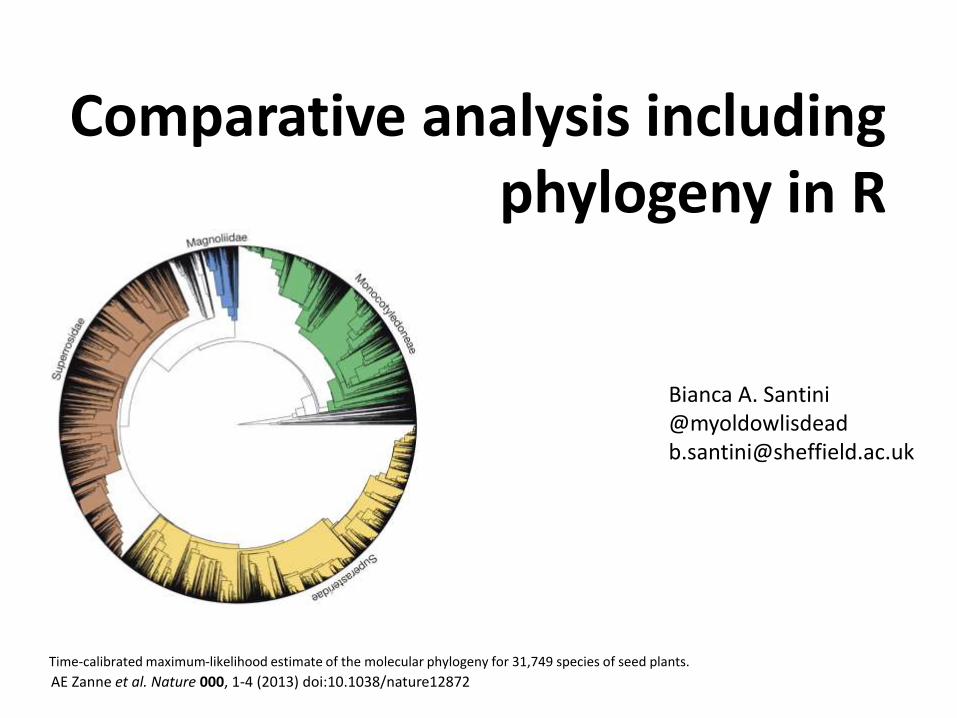
Comparative analysis including phylogeny in R
AE Zanne et al. Nature 000, 1-4 (2013) doi:10.1038/nature12872
Time-calibrated maximum-likelihood estimate of the molecular phylogeny for 31,749 species of seed plants.
Bianca A. [email protected]@sheffield.ac.uk

What is a phylogeny?
• Hypothesis that explains the evolutionary relationship among taxa*
*taxa: species, or higher taxonomic levels.
Also genes, or sequences
node
terminals/tips/leaves
root
A B C
D
Internal branch
branch
External branch
Mo
dif
ied
fro
m N
atu
re S
cita
ble
: h
ttp
://w
ww
.nat
ure
.co
m/s
cita
ble
/to
pic
pag
e/re
adin
g-a-
ph
ylo
gen
etic
-tr
ee-t
he-
mea
nin
g-o
f-4
19
56
#

Why use phylogenies… …in comparative analysis?
• Comparative analyses are used to assess the ecological significance of a particular trait
• However, because there is a shared history…
a) they are not statistically independent data
b) the feature under study might exist
because of shared ancestry

One example of data analyzed without a phylogeny
• Salisbury’s data (1927, yes 88yrs ago!)
• Observations
– Differences in stomata density (SD) between sun(>) and shade (<) leaves
• Measured stomatal density and related them to life-form, habitat type
• Conclusion: SD increases with exposure
SD
Trees Shrubs Herbs Woody Herbsplants
SD
Marginalherbs
Understoryherbs
Photo by A. Vazquez-Lobo

Re-analysis of Salisbury’s data
• Independent contrasts (Felsenstein, 1985)– Introduces a phylogeny
– The trait changes along the branches of the tree, should be associated to changes in the explanatory variable
– no. of times the traits changes in concert with the environmental variable (agreements)
vs.
no. of times they do not (disagreements)
– Sign test
SD
Trees Shrubs Herbs Woody Herbsplants
SD
Marginalherbs
Understoryherbs
Kelly and Beerling, 1995 (68 yrs after)

How to get your own phylogeny ?
phylomatic (uses a megatree)
http://phylodiversity.net/phylomatic/
Use and trim and already published phylogeny:
- Dryad: http://datadryad.org/- Ecological Archives (from the esa)
phyloGenerator (uses gen bank sequences) http://willpearse.github.io/phyloGenerator/
This is if you don’t have the sequences, or are not planning to get them.

Package CAPER : pgls()Similar approach as in Independent Contrasts, but uses a matrix
of variances and covariances (tree)
N.B. If interested in phylogenies and evolution analyses: geiger, adephylo, picante, phylolm, ape…
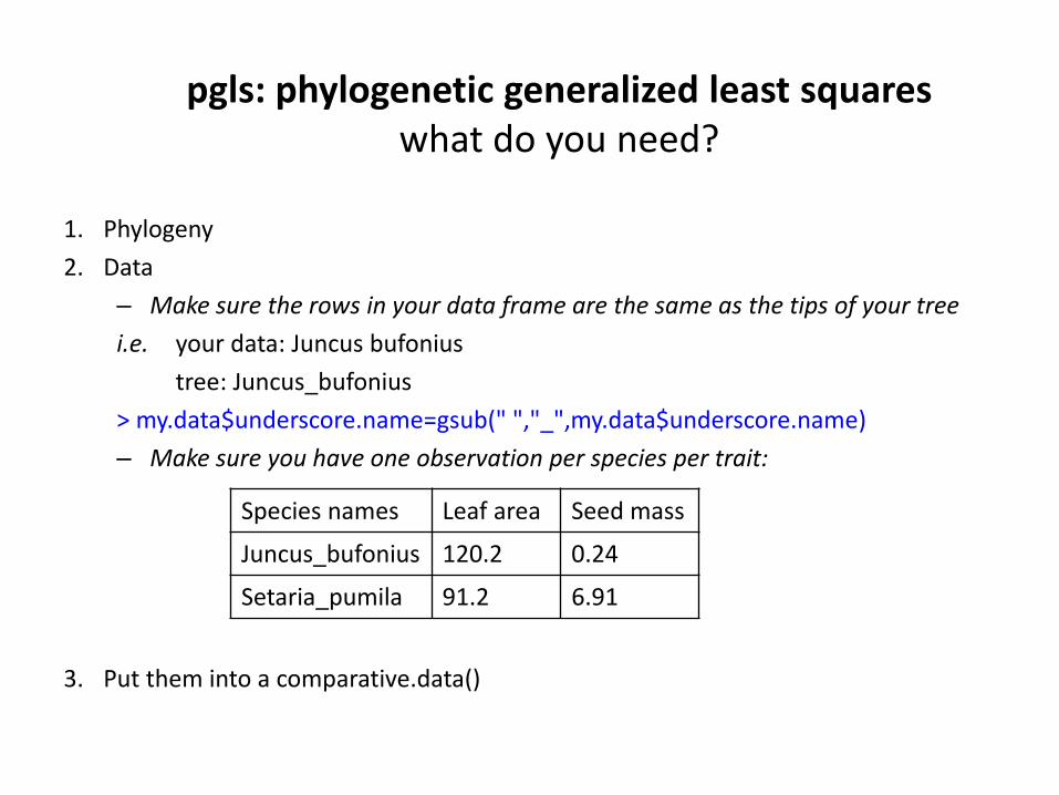
pgls: phylogenetic generalized least squareswhat do you need?
1. Phylogeny
2. Data
– Make sure the rows in your data frame are the same as the tips of your tree
i.e. your data: Juncus bufonius
tree: Juncus_bufonius
> my.data$underscore.name=gsub(" ","_",my.data$underscore.name)
– Make sure you have one observation per species per trait:
3. Put them into a comparative.data()
Species names Leaf area Seed mass
Juncus_bufonius 120.2 0.24
Setaria_pumila 91.2 6.91

#1)PHYLOGENY > tree<-read.tree ("Vascular_Plants_rooted.dated.tre”) ##or read.nexus()
> tree <- congeneric.merge(tree,my.data$underscore.name) ##pez package
Number of species in tree before: 401
Number of species in tree now: 550
> treePhylogenetic tree with 550 tips and 393 internal nodes.
Tip labels:
Gladiolus_italicus, Juncus_squarrosus, Juncus_bufonius, Bolboschoenus_maritimus, Isolepis_setacea, Cyperus_fuscus, ...
Node labels:
, , , , , , …
Rooted; includes branch lengths.
pgls()
#You can always check for synonyms and replace (taxize)> my.data$underscore.name<-recode(my.data$underscore.name, "'Aegilops_geniculata' = 'Aegilops_ovata'")
> plot.phylo(tree, cex=0.45, type="radial", edge.color=c("red", "orange", "blue"))

pgls()
##trim your tree> tree <- drop.tip(tree, setdiff(tree$tip.label, my.data$underscore.name))
#2) YOUR DATA> dat<-data.frame(read.csv(“mydata.csv",header=T))
#3)PUT THEM together in comparative data, which will drop rows with NAs for you and match the rows to the tips of the phylogeny :D > cdat <- comparative.data(data = dat, phy = tree, names.col = ”underscore.name”, scope=leaf.area~seed.mass, vcv=TRUE) #na.omit=FALSE #warn.dropped=TRUE
> cdat$dropped #to see what has been dropped.
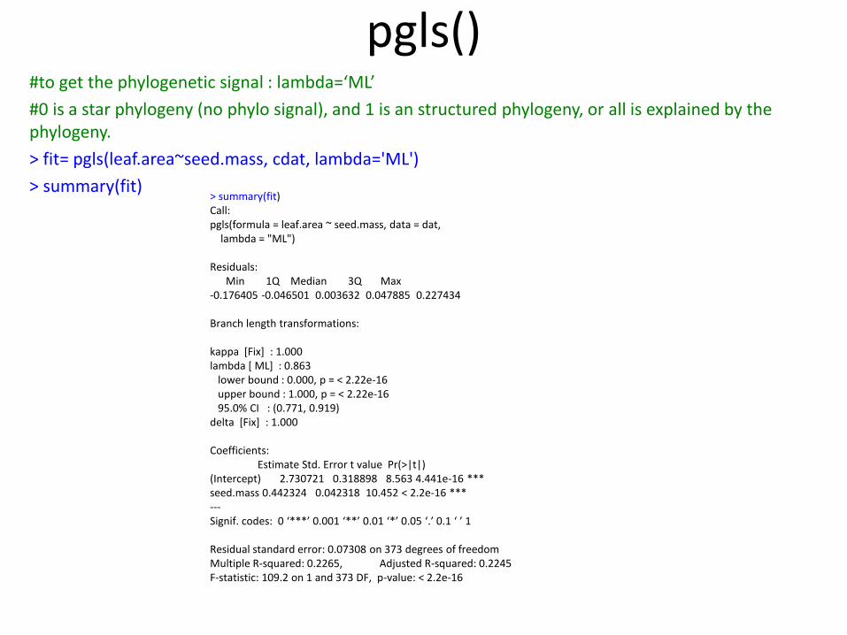
#to get the phylogenetic signal : lambda=‘ML’
#0 is a star phylogeny (no phylo signal), and 1 is an structured phylogeny, or all is explained by the phylogeny.
> fit= pgls(leaf.area~seed.mass, cdat, lambda='ML')
> summary(fit)
pgls()
> summary(fit)Call:pgls(formula = leaf.area ~ seed.mass, data = dat,
lambda = "ML")
Residuals:Min 1Q Median 3Q Max
-0.176405 -0.046501 0.003632 0.047885 0.227434
Branch length transformations:
kappa [Fix] : 1.000lambda [ ML] : 0.863
lower bound : 0.000, p = < 2.22e-16upper bound : 1.000, p = < 2.22e-1695.0% CI : (0.771, 0.919)
delta [Fix] : 1.000
Coefficients:Estimate Std. Error t value Pr(>|t|)
(Intercept) 2.730721 0.318898 8.563 4.441e-16 ***seed.mass 0.442324 0.042318 10.452 < 2.2e-16 ***---Signif. codes: 0 ‘***’ 0.001 ‘**’ 0.01 ‘*’ 0.05 ‘.’ 0.1 ‘ ’ 1
Residual standard error: 0.07308 on 373 degrees of freedomMultiple R-squared: 0.2265, Adjusted R-squared: 0.2245 F-statistic: 109.2 on 1 and 373 DF, p-value: < 2.2e-16

But what if you want to analyze factors?
#CAPER has some bugs…
> cdat <- comparative.data(data = dat, phy = tree, names.col = ”underscore.name”,scope = leaf area ~nitro.class, vcv=TRUE)
> fit= pgls(leaf area ~nitro.class, cdat, lambda='ML')
> anova(fit)
Error in terms.formula(formula,data=data):
invalid model formula in ExtractVars
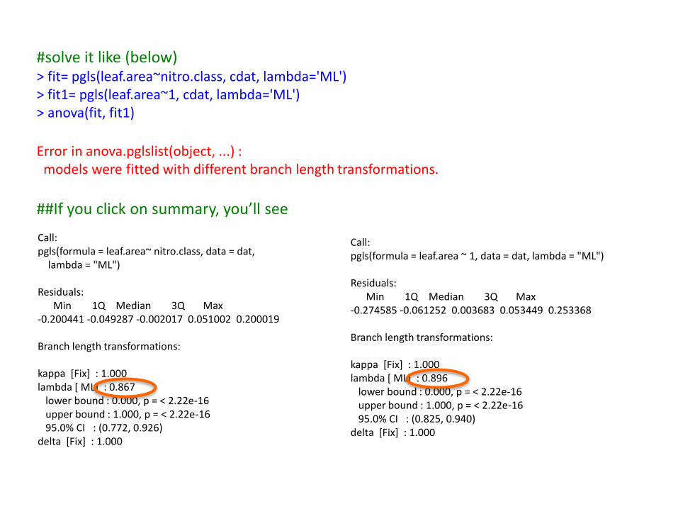
#solve it like (below) > fit= pgls(leaf.area~nitro.class, cdat, lambda='ML')> fit1= pgls(leaf.area~1, cdat, lambda='ML')> anova(fit, fit1)
Error in anova.pglslist(object, ...) : models were fitted with different branch length transformations.
##If you click on summary, you’ll see
Call:pgls(formula = leaf.area~ nitro.class, data = dat,
lambda = "ML")
Residuals:Min 1Q Median 3Q Max
-0.200441 -0.049287 -0.002017 0.051002 0.200019
Branch length transformations:
kappa [Fix] : 1.000lambda [ ML] : 0.867
lower bound : 0.000, p = < 2.22e-16upper bound : 1.000, p = < 2.22e-1695.0% CI : (0.772, 0.926)
delta [Fix] : 1.000
Call:pgls(formula = leaf.area ~ 1, data = dat, lambda = "ML")
Residuals:Min 1Q Median 3Q Max
-0.274585 -0.061252 0.003683 0.053449 0.253368
Branch length transformations:
kappa [Fix] : 1.000lambda [ ML] : 0.896
lower bound : 0.000, p = < 2.22e-16upper bound : 1.000, p = < 2.22e-1695.0% CI : (0.825, 0.940)
delta [Fix] : 1.000
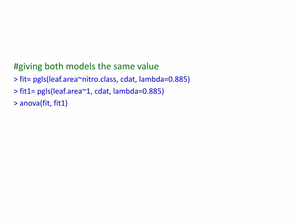
#giving both models the same value> fit= pgls(leaf.area~nitro.class, cdat, lambda=0.885)
> fit1= pgls(leaf.area~1, cdat, lambda=0.885)
> anova(fit, fit1)

You can also use gls(), instead of lambda do method=‘ML’
Visualize your tree, always exciting!
In R
> plot(tree)
> help(plot.phylo) #install ape
#and: http://www.r-phylo.org/wiki/Main_Page
Use FigTree (drop the file and it will do the phylogeny for you)
phytools

>plot.phylo(tree, cex=0.3)
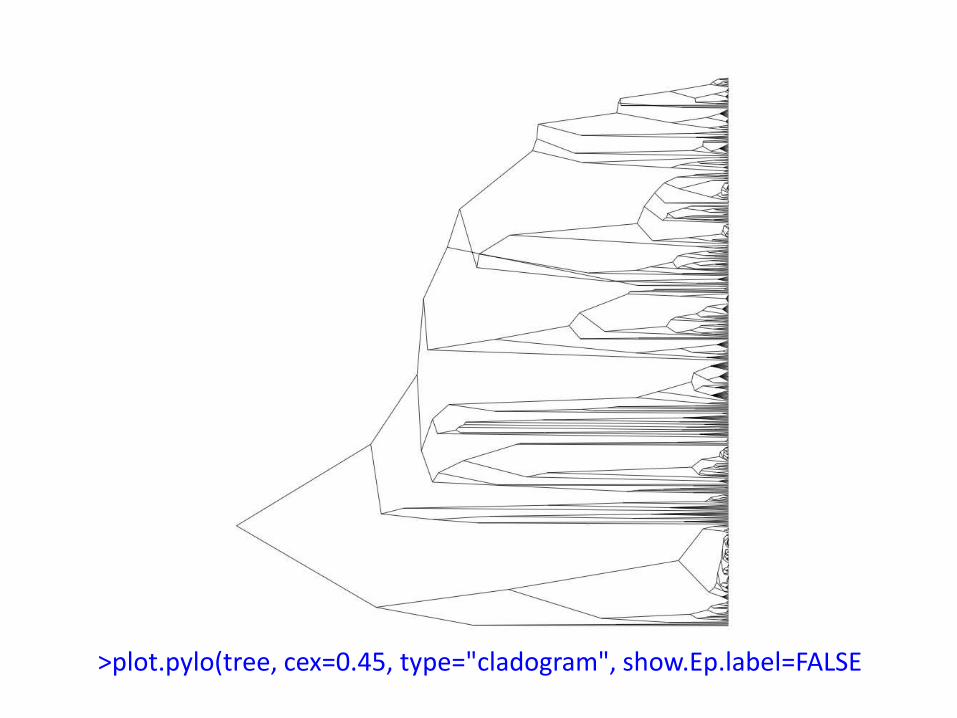
>plot.pylo(tree, cex=0.45, type="cladogram", show.Ep.label=FALSE

>plot.phylo(tree, cex=0.45, type="fan", edge.color=c("red", "orange", "green","blue"), edge.lty=5)

From Freckleton et al. 2002.