
Persuasion and Information Aggregation in Elections
80
Persuasion and Information Aggregation in Elections * Carl Heese † Stephan Lauermann ‡ August 18, 2021 Abstract This paper studies a large majority election with voters who have het- erogeneous, private preferences and exogenous private signals. We show that a Bayesian persuader can implement any state-contingent outcome in some equilibrium by providing additional information. In this setting, with- out the persuader’s information, a version of the Condorcet Jury Theorem holds (Feddersen and Pesendorfer, 1997). Persuasion does not require de- tailed knowledge of the voters’ private information and preferences: the same additional information is effective across environments. The results require almost no commitment power by the persuader. Finally, the per- suasion mechanism is effective also in small committees with as few as 15 members. In most elections, a voter’s ranking of outcomes depends on her information. For example, a shareholder’s view of a proposed merger depends on her belief re- garding its profitability, and a legislator’s support of proposed legislation depends on her belief regarding its effectiveness. An interested party that has private infor- mation may utilize this fact by strategically releasing information to affect voters’ * We are grateful for helpful discussions with Ricardo Alonso, Nageeb Ali, Arjada Bardhi, Dirk Bergemann, Sourav Bhattacharya, Francesc Dilme, Mehmet Ekmekci, Erik Eyster, Tim Feddersen, Yingni Guo, Matt Jackson, Daniel Kr¨ ahmer, Elliot Lipnowski, Antonio Penta, Ja- copo Perego, Keith Schnakenberg, and Thomas Tr¨ oger, as well as comments from audiences at Oxford, Bonn, Yale (lunch), LSE (lunch), ESWM 2017, CRC TR224 Conference 2018, SAET 2018, ESEM 2018, ASSA meetings 2019 Atlanta, and the annual Wallis Institute conference. This work was supported by a grant from the European Research Council (ERC 638115) and the Deutsche Forschungsgemeinschaft (DFG, German Research Foundation) under Germanys Excellence Strategy EXC 2126/1-390838866 and through the CRC TR 224 (Project B03 and B04). † University of Vienna, Department of Economics, [email protected] ‡ University of Bonn, Department of Economics, [email protected]. 1
Transcript of Persuasion and Information Aggregation in Elections
Persuasion and Information Aggregation in
Elections ∗
Carl Heese † Stephan Lauermann ‡
August 18, 2021
Abstract
This paper studies a large majority election with voters who have het-erogeneous, private preferences and exogenous private signals. We showthat a Bayesian persuader can implement any state-contingent outcome insome equilibrium by providing additional information. In this setting, with-out the persuader’s information, a version of the Condorcet Jury Theoremholds (Feddersen and Pesendorfer, 1997). Persuasion does not require de-tailed knowledge of the voters’ private information and preferences: thesame additional information is effective across environments. The resultsrequire almost no commitment power by the persuader. Finally, the per-suasion mechanism is effective also in small committees with as few as 15members.
In most elections, a voter’s ranking of outcomes depends on her information.
For example, a shareholder’s view of a proposed merger depends on her belief re-
garding its profitability, and a legislator’s support of proposed legislation depends
on her belief regarding its effectiveness. An interested party that has private infor-
mation may utilize this fact by strategically releasing information to affect voters’
∗We are grateful for helpful discussions with Ricardo Alonso, Nageeb Ali, Arjada Bardhi,Dirk Bergemann, Sourav Bhattacharya, Francesc Dilme, Mehmet Ekmekci, Erik Eyster, TimFeddersen, Yingni Guo, Matt Jackson, Daniel Krahmer, Elliot Lipnowski, Antonio Penta, Ja-copo Perego, Keith Schnakenberg, and Thomas Troger, as well as comments from audiences atOxford, Bonn, Yale (lunch), LSE (lunch), ESWM 2017, CRC TR224 Conference 2018, SAET2018, ESEM 2018, ASSA meetings 2019 Atlanta, and the annual Wallis Institute conference.This work was supported by a grant from the European Research Council (ERC 638115) andthe Deutsche Forschungsgemeinschaft (DFG, German Research Foundation) under Germany´sExcellence Strategy EXC 2126/1-390838866 and through the CRC TR 224 (Project B03 andB04).
† University of Vienna, Department of Economics, [email protected]‡ University of Bonn, Department of Economics, [email protected].
1
behavior. Examples of interested parties holding and strategically releasing rele-
vant information for voters are numerous: in a shareholder vote, the management
may strategically provide information regarding the merger through presentations
and conversations; similarly, lobbyists provide selected information to legislators
to influence their votes.
We are interested in the scope of such “persuasion” (Kamenica and Gentzkow,
2011) in elections. We study this question in the canonical voting setting by
Feddersen and Pesendorfer (1997): There are two possible policies (outcomes)—
A and B. Voters’ preferences over policies are heterogeneous and depend on an
unknown state, α or β, in a general way (some voters may prefer A in state
α, some prefer A in state β, and some “partisans” may prefer one of the policies
independently of the state). The preferences are drawn independently across voters
and are each voters’ private information. In addition, all voters privately receive
information in the form of a noisy signal. The election determines the outcome
by a simple majority rule.
In this setting, Feddersen and Pesendorfer (1997) have shown that within a
broad class of “monotone” preferences and conditionally i.i.d. private signals,
all equilibrium outcomes of large elections are equivalent to the outcome with a
publicly known state (“information aggregation”). We restate their result as a
benchmark in Theorem 1.
We ask the following question: can a manipulator ensure that a majority
supports his favorite policy—potentially state-dependent—in a large election by
providing additional information to the voters? Formally, the manipulator can
choose and commit to any joint distribution over states and signal realizations
that are then privately observed by the voters. In particular, the manipulator’s
additional signal is required to be independent of the voters’ exogenous private
signals and their individual preferences (it is an “independent expansion”). The
previous result by Feddersen and Pesendorfer (1997) suggests a limited scope for
persuasion because, if voters simply ignored the additional information, the out-
come would be “as if” the state were known, and, hence, the information provided
by the manipulator would be worthless.
Our main result (Theorem 4) shows that, perhaps surprisingly, within the same
class of monotone preferences and for any state-contingent policy, there exists an
independent expansion of the voters’ exogenous i.i.d. signal and an equilibrium
that ensures that the targeted policy is supported by a majority with probability
close to one when the number of voters is large. Thus, just by providing additional
2
information, a manipulator can implement, for example, a targeted policy that is,
in every state, the opposite of the outcome with full information.
The additional information affects the voters’ behavior in two ways: directly,
by changing their beliefs about the state, and indirectly, by affecting their inference
from being “pivotal” for the election outcome. While the direct effect is limited by
the well-known “Bayesian-consistency” requirement of beliefs, the pivotal inference
turns out to have no such constraint.
To explain the effectiveness of persuasion, we first consider the case in which all
information of the voters comes from a manipulator (“monopolistic persuasion”).
To invert the full information outcome, the manipulator can choose an information
structure in which, roughly speaking, signals are of two possible qualities: revealing
or obfuscating. When the signal is revealing, all voters observe the same signal, a
in state α and b in state β. The signal is revealing with probability 1− ε. Thus,
when ε = 0, the election leads to the full information outcome.
However, with probability ε, the signal is obfuscating. In this case, in both
states, almost all voters receive an uninformative signal z while a few voters receive
an “erroneous” signal, that is, they receive a in β and b in α. Hence, in this
situation, a and b carry the opposite meaning from before.
What matters for the persuasion logic is that voters react to the closeness of the
election. The closeness of the election tells voters something about the quality of
the information of the others, and, in this way, also something about the quality of
their own signal. In the equilibrium that we construct, a close election will imply
that the signal of the others is of low quality (obfuscating), meaning that almost
all received signal z, and, in this case, the meaning of an otherwise strong signal
a in favor of α will be different and interpreted as being in favor of β, and vice
versa for b.
A numerical example with 15 voters illustrates the persuasion logic. The con-
struction uses the exact same fixed-point argument as the general analysis, show-
ing that the same mechanism is already effective in small elections; see Section
4.3. Thus, even though we utilize large numbers in our formal statements, our
results may also be relevant for committees with a small or intermediate number
of members.
We argue the robustness of the persuasion logic by addressing common con-
cerns regarding the sender’s commitment power, equilibrium coordination of the
receivers, and the dependence of the mechanism on details of the environment.
We show that the sender needs very little commitment power. To model partial
3
commitment, we follow the existing literature (see e.g. Lipnowski, Ravid, and
Shishkin (2019)): The sender is committed only with probability 1−χ, and, with
probability χ, he is free to send any signals. We show that the sender can persuade
a large electorate (Proposition 1) even for arbitrarily small χ > 0.
The manipulated equilibrium has desirable properties that may facilitate the
coordination on this equilibrium. First, the equilibrium is “attracting.” In partic-
ular, its “basin of attraction” for the iterated best response dynamic is essentially
the full set of strategy profiles: if we begin with almost any strategy profile and
consider, first, the voters’ best response to it and then the voters’ best response
to this best response, then the resulting strategy profile is arbitrarily close to the
manipulated equilibrium when the number of voters is large (Proposition 3). Nev-
ertheless, we show that, given the information structure, there is also one other
equilibrium that yields the full-information outcome (Theorem 3). Second, the
behavior in the manipulated equilibrium is based on a simple line of reasoning.
In particular, voters will only need to interpret their own signal conditional on
it being “obfuscating,” and behave optimally given this interpretation (akin to
so-called “sincere voting”). By contrast, any other equilibrium hinges on detailed
calculations of pivotal likelihoods.1
We show that the same information structure can be used uniformly across
many environments, that is, the signal does not need to be tailored to the details
of the game (Wilson, 1987, “Wilson doctrine”): for any target policy, there exists
a single information structure that implements the policy for any prior about the
state and preference distribution of the voters that satisfy a weak condition; see
Proposition 2.
In the second part of the paper, we consider the setting in which voters al-
ready have access to exogenous information of the form studied in Feddersen and
Pesendorfer (1997). We show that, by adding information with the same signal
structure as before to the exogenous information, the manipulator can still per-
suade the voters effectively to elect any state-contingent policy (Theorem 4). In
particular, the additional signal structure also does not need to be finely tuned to
the details of the environment and is effective independent of the voters’ private
information. Furthermore, it is sufficient if the sender has partial information
about the state in the form of a private signal (Section 7.1).
In Section 6, we provide a stylized application to media markets. This serves
two purposes: First, we show that the main results of the paper can also be
1In Section 4.6.4, we also briefly discuss a model with some behavioral types who do notcondition on being pivotal, following Kawai and Watanabe (2013).
4

obtained in a setting with normally distributed voter information. Second, within
the application, we can discuss concrete strategies of information manipulation.
In Section 8, we discuss the paper’s contribution to the existing literature on
information aggregation in elections and on voter persuasion, especially the work
by Wang (2013), Alonso and Camara (2016), Chan, Gupta, Li, and Wang (2019)
and Bardhi and Guo (2018). This literature observed in particular that, with mul-
tiple receivers, the conditioning on being pivotal weakens the Bayesian consistency
constraint. In contrast to this prior work, which assumes that the voters’ prefer-
ences and information are commonly known, we allow for heterogeneous, privately
known preferences and exogenous information. On the one hand, this allows cap-
turing the canonical environment by Feddersen and Pesendorfer (1997) in which,
otherwise, equilibrium implies the full-information outcome. On the other hand,
the persuasion mechanism here is distinct from the persuasion logic when voters’
preferences are commonly known and voters can be targeted individually, as illus-
trated in an example in Section 7.2. Moreover, we show that voter persuasion is
robust in several dimensions (limited commitment, equilibrium coordination, and
detail-freeness).
We note two broader implications of our analysis. First, it may be difficult
for an outside observer to make a “robust” prediction. If an observer knows that
voters have access to at least the information assumed in Feddersen and Pesendor-
fer (1997), but cannot exclude that voters have access to additional information
of the type discussed here, then no outcome can be excluded as an equilibrium
prediction. Second, if one interprets an information structure with a small ε as a
small departure from common knowledge, our result adds another observation to
the literature on the effects of strategic uncertainty (Weinstein and Yildiz, 2007).
The proof for the main result with a monopolistic sender, Theorem 2, is in the
main body and the appendix. The proofs for the other results are sketched here;
details are relegated to an online appendix.
1 Model
There are 2n+ 1 voters (or citizens), two policies, A and B, and two states of the
world, ω ∈ {α, β}. The prior probability of α is Pr (α) ∈ (0, 1).
Voters have heterogeneous preferences. A voter’s preference is described by a
type t = (tα, tβ) ∈ [−1, 1]2, with tω being the utility of A in ω. The utility of B
is normalized to zero; so, tω is the difference of the utilities from A and B in ω.
5
The types are independently and identically distributed across voters according
to a cumulative distribution function G : [−1, 1]2 → [0, 1], with a strictly positive,
continuous density g. The own type is the private information of the voter.
An information structure π is a finite set of signals S and a joint distribution
of signal profiles and states that is independent of G. The conditional distribu-
tion is exchangeable with respect to the voters. In particular, there is a finite
number of substates {αj}j=1,...,Nαand {βj}j=1,...,Nβ
, such that the signals are in-
dependently and identically distributed conditional on the substates.2 Abusing
notation slightly, Pr(ωj|ω) and Pr(si|ωj) denote the corresponding probabilities of
the substates and the individual signal si, conditional on a substate. Thus, the
probability of the signal profile s = (si)i=1,...,2n+1 ∈ S2n+1 is
Pr(s|ω) =∑j
Pr(ωj|ω)∏
i=1,...,2n+1
Pr(si|ωj). (1)
The observed signal is the private information of the voter.
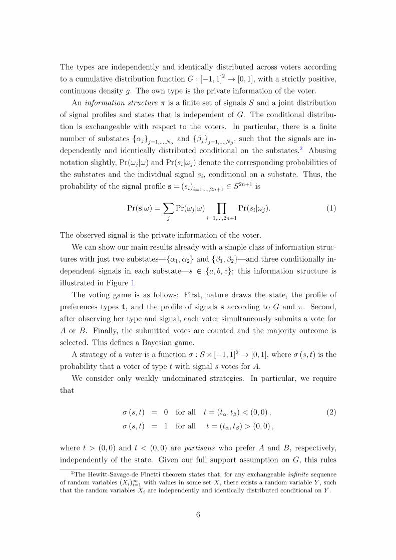
We can show our main results already with a simple class of information struc-
tures with just two substates—{α1, α2} and {β1, β2}—and three conditionally in-
dependent signals in each substate—s ∈ {a, b, z}; this information structure is
illustrated in Figure 1.
The voting game is as follows: First, nature draws the state, the profile of
preferences types t, and the profile of signals s according to G and π. Second,
after observing her type and signal, each voter simultaneously submits a vote for
A or B. Finally, the submitted votes are counted and the majority outcome is
selected. This defines a Bayesian game.
A strategy of a voter is a function σ : S× [−1, 1]2 → [0, 1], where σ (s, t) is the
probability that a voter of type t with signal s votes for A.
We consider only weakly undominated strategies. In particular, we require
that
σ (s, t) = 0 for all t = (tα, tβ) < (0, 0) , (2)
σ (s, t) = 1 for all t = (tα, tβ) > (0, 0) ,
where t > (0, 0) and t < (0, 0) are partisans who prefer A and B, respectively,
independently of the state. Given our full support assumption on G, this rules
2The Hewitt-Savage-de Finetti theorem states that, for any exchangeable infinite sequenceof random variables (Xi)
∞i=1 with values in some set X, there exists a random variable Y , such
that the random variables Xi are independently and identically distributed conditional on Y .
6

Figure 1: The main class of information structures considered in this paper.Each state ω has two substates {ω1, ω2}, occurring with conditional probabili-ties Pr(ωj|ω). Conditional on the substate ωj, the distribution of the signalssi ∈ {a, z, b} is independent and identical with the marginal probabilities denotedby Pr(s|ωj) (these marginals are degenerate in α1 and β1) .
out degenerate strategies for which either σ (s, t) = 1 for all (s, t) or σ (s, t) = 0
for all (s, t). Here, and in the following, we ignore zero measure sets when writing
“for all”.
From the viewpoint of a given voter and given any strategy σ′ used by the
other voters, the pivotal event piv is the event in which the realized types and
signals of the other 2n voters are such that exactly n of them vote for A and n for
B. In this event, if she votes A, the outcome is A; if she votes B, the outcome is
B. In any other event, the outcome is independent of her vote. Thus, a strategy
is optimal if and only if it is optimal conditional on the pivotal event.
Let Pr(α|s, piv;σ′) denote the posterior probability of α conditional on s and
conditional on being pivotal, given the measure induced by the nondegenerate
strategy σ′. The strategy σ is a best response to σ′ if and only if
Pr(α|s, piv;σ′) · tα + (1− Pr(α|s, piv;σ′)) · tβ > 0⇒ σ (s, t) = 1, (3)
and
Pr(α|s, piv;σ′) · tα + (1− Pr(α|s, piv;σ′)) · tβ < 0⇒ σ (s, t) = 0, (4)
that is, a voter supports A if the expected value of A conditional on being pivotal
is strictly positive, and a voter supports B otherwise. Note that indifference holds
7

only for a set of types that has zero measure. For all other types, the best response
is pure. It follows that there is no loss of generality to consider pure strategies
with σ (s, t) ∈ {0, 1} for all (s, t).
Thus, a symmetric, undominated, and pure Bayes-Nash equilibrium of Γ(π) is
a strategy σ : S × [−1, 1]2 → {0, 1} that satisfies (2), (3), and (4), with σ′ = σ.
We refer to such a strategy simply as an equilibrium.
2 Preliminary Observations
2.1 Inference from the Pivotal Event
When making an inference from being pivotal, voters ask which state is more likely
conditional on a tie, with exactly n voters supporting A and n supporting B. It
is intuitive that a tie is evidence in favor of the substate in which the election is
closer to being tied in expectation. Thus, conditional on being pivotal, a voter
updates toward the substate in which the expected vote share is closer to 12. We
now verify this simple intuition and introduce some notation along the way.
For a strategy σ, the probability that a voter supports A in substate ωj is
q (ωj;σ) =∑s∈S
Pr (s|ωj) PrG ({t : σ (s, t) = 1}), (5)
where q (ωj;σ) is the expected vote share of A.
Given that the signals and the types of the voters are independent conditional
on the substate, the probability of a tie in the vote count is
Pr (piv|ωj;σ) =
(2n
n
)(q (ωj;σ))n (1− q (ωj;σ))n . (6)
For any two substates ωj and ωl, the likelihood ratio of being pivotal is
Pr (piv|ωj;σ)
Pr (piv|ωl;σ)=
(q (ωj;σ) (1− q (ωj;σ))
q (ωl;σ) (1− q (ωl;σ))
)n. (7)
Using the conditional independence, the posterior likelihood ratio of any two sub-
states conditional on a signal s and the event that the voter is pivotal is
Pr (ωj|piv, s;σ)
Pr (ωl|piv, s;σ)=
Pr(ωj)
Pr(ωl)
Pr(s|ωj)Pr(s|ωl)
Pr (piv|ωj;σ)
Pr (piv|ωl;σ). (8)
8

We record the intuitive fact that voters update toward the substate in which
the vote share is closer to 1/2, that is, the substate in which the election is closer
to being tied in expectation.
Claim 1 Take any two substates ωj and ωl, and any strategy σ for which Pr (piv|ωl;σ) ∈(0, 1); if ∣∣∣∣q (ωj;σ)− 1
2
∣∣∣∣ < ∣∣∣∣q (ωl;σ)− 1
2
∣∣∣∣ , (9)
thenPr (piv|ωj;σ)
Pr (piv|ωl;σ)> 1. (10)
Proof. The function q(1 − q) has an inverse u-shape on [0, 1] and is symmetric
around its peak at q = 12. So,
∣∣q − 12
∣∣ < ∣∣q′ − 12
∣∣ implies that q(1− q) > q′(1− q′).Thus, it follows from (7) that (9) implies (10).
2.2 Pivotal Voting
Given any strategy profile σ′ used by the others, the vector of posteriors conditional
on piv and s is denoted as
ρ (σ′) = (Pr(α|s, piv;σ′))s∈S. (11)
This vector of posteriors is a sufficient statistic for the unique best response to σ′
for all nonpartisan voter types; see (3) and (4).
Thus, given some arbitrary vector of beliefs p =(ps)s∈S , let σp be the unique
undominated strategy that is optimal if a voter with a signal s believes the prob-
ability of α to be ps. That is, for all (s, t),
σp (s, t) = 1⇔ ps · tα + (1− ps) · tβ > 0, (12)
and (2) holds for the partisans.
The strategy σ is a best response to σ′ if and only if σ = σp for p = ρ (σ′).
Thus, σ∗ is an equilibrium if and only if σ∗ = σρ(σ∗). Conversely, an equilibrium
can be described by a vector of beliefs p∗ that is a fixed point of ρ(σp), that is
p∗ = ρ (σp∗) ; (13)
meaning, the belief p∗ corresponds to an equilibrium if, when voters behave op-
timally given p∗ (i.e., vote according to σp∗), the posterior conditional on being
9

pivotal is again p∗.
Equation (13) provides an equilibrium existence argument: the expression
ρ (σp) defines a finite-dimensional mapping [0, 1]|S| → [0, 1]|S| from beliefs p into
posterior beliefs ρ (σp), and this mapping is continuous.3 Thus, an application
of Kakutani’s theorem implies the existence of a fixed point p∗ that solves (13).4
The strategy σp∗ is an equilibrium.5
The possibility of writing equilibria in terms of posteriors enables us to connect
our model and results to the Bayesian persuasion literature.
2.3 Aggregate Preferences
A central object of the analysis is the aggregate preference function,
Φ(p) := PrG({t : p · tα + (1− p) · tβ > 0}), (14)
which maps a belief p ∈ [0, 1] to the probability that a random type t prefers
A under p. The function Φ proves useful to express expected vote shares: if a
strategy σ is optimal given beliefs p—i.e., σ = σp— then the expected vote share
of outcome A in substate ωj is
q (ωj;σ) =∑s∈S
Pr(s|ωj)Φ (ps) . (15)
Figure 2 illustrates Φ. Given p, the dashed (blue) line corresponds to the plane of
indifferent types t = (tα, tβ) with p · tα + (1 − p) · tβ = 0. Voters having types to
the north-east prefer A given p, and Φ is the measure of such types under G. The
indifference plane has a slope − p1−p , and a change in p corresponds to a rotation
of it. Given that G has a continuous density, it follows that the function Φ is
continuous in p. Given that G has a strictly positive density on [−1, 1]2, we also
have that
0 < Φ(p) < 1 for all p ∈ [0, 1]. (16)
As observed earlier, voters having types t in the north-east quadrant prefer A
3To see why ρ (σp) is continuous in p, first, note that (12) implies that PrG({t : σp (s, t) = 1})is continuous in p since G has a continuous density. Second, q(ωj ;σ
p) is continuous inPrG({t : σp (s, t) = 1}), given (5). Third, ρ(σp) is continuous in q(ωj ;σ
p), given (6) and (8).4The ability to write an equilibrium as a finite-dimensional fixed point via (13) is a significant
advantage. Similar reductions to finite dimensional equilibrium beliefs have been used in relatedvoting settings previously (see Bhattacharya, 2013; Ahn and Oliveros, 2012).
5Note that, because of the partisans, σp∗is non-degenerate.
10

−1 1
−1
1
tβ = −p1−ptα
tα
tβ
Figure 2: The plane of indifferent types is tβ = −p1−ptα for any given belief p =
Pr(α) ∈ (0, 1).
for all beliefs and voters having types t in the south-west quadrant always prefer B
(partisans). Voters having types t in the south-east quadrant prefer A in state α
and B in β (aligned voters), and voters having types t in the north-west quadrant
prefer B in state α and A in β (contrarian voters).
We assume throughout the paper that the distribution of types is sufficiently
rich so that there is a belief p for which a majority prefers A and a belief p′ for
which a majority prefers B,6 that is,
Φ (p′) <1
2< Φ (p) . (17)
3 Large Elections: Basic Results
We consider a sequence of elections along which the electorate’s size n grows.
For each 2n + 1, we fix some strategy profile σn and calculate the probability
that a policy x ∈ {A,B} wins the support of the majority of the voters in state
ω, denoted Pr (x|ω;σn, n). We are interested in the limit of Pr (x|ω;σ∗n, n), as
n → ∞, for equilibrium sequences (σ∗n)n∈N. We first state a central observation
regarding the inference from being pivotal in large elections; we then show how
this observation implies the “modern” Condorcet Jury Theorem (CJT), which we
restate as a benchmark.
6Otherwise, the analysis is trivial. If, for all beliefs p ∈ [0, 1], in expectation a majorityprefers A, then, for any information structure, the vote share of A is larger than 1
2 , and A winsin every large election.
11

3.1 Inference in Large Elections
As a first step, we study the properties of the inference from being pivotal in a
large election. We show that Claim 1 extends in an extreme form as the electorate
grows large (n → ∞): The event that the election is tied is infinitely more likely
in the (sub-)state in which the election is closer to being tied in expectation. In
fact, the likelihood ratio of the pivotal event diverges exponentially fast.
Because we want to allow the information structure to depend on n, we also
include πn in the argument. The set of substates remains fixed.
Claim 2 Consider any sequence of strategies (σn)n∈N, any sequence of informa-
tion structures (πn)n∈N, and any two substates ωj and ωl for which Pr (piv|ωl;σ, n, πn) ∈(0, 1) for all n. If
limn→∞
∣∣∣∣q (ωj;σn, πn)− 1
2
∣∣∣∣ < limn→∞
∣∣∣∣q (ωl;σn, πn)− 1
2
∣∣∣∣ , (18)
then, for any d ≥ 0,
limn→∞
Pr (piv|ωj;σn, πn)
Pr (piv|ωl;σn, πn)n−d =∞. (19)
Proof. Let
kn =q (ωj;σn, πn)
q (ωj;σn, πn)
(1− q (ωj;σn, πn))
(1− q (ωj;σn, πn)).
From (7), the left-hand side of (19) is (kn)n
nd. If (18) holds, then limn→∞ kn > 1,
because of the properties of q (1− q) (inverse u-shaped around 1/2). Therefore,
limn→∞ (kn)n =∞. Moreover, (kn)n diverges exponentially fast and, hence, dom-
inates the denominator nd, which is polynomial.
3.2 Benchmark: Condorcet Jury Theorem
The model embeds a special case of the canonical voting game by Feddersen and
Pesendorfer (1997) with a binary state. In the following, we restate their full-
information equivalence result, assuming, at first, that signals are binary with
S = {u, d}.As in Feddersen and Pesendorfer (1997), we assume that the signals are in-
dependently and identically distributed across voters conditional on the state
ω ∈ {α, β}.7 This corresponds to the case of an information structure πc with
7Feddersen and Pesendorfer (1997) assume the existence of subpopulations and allow the
12

a single substate in each state; in the following, we identify the substate with this
state. The probabilities Pr(s|ω; πc) for s ∈ {u, d} and ω ∈ {α, β} satisfy
1 > Pr(u|α; πc) > Pr(u|β; πc) > 0 ; (20)
that is, signal u is indicative of α, and signal d is indicative of β. We further
assume that
Φ(p) is strictly increasing in p. (21)
We say that the aggregate preference function is monotone.8 Monotonicity (21)
and (17) together imply that Φ(0) < 12< Φ(1); thus, the full information outcome
is A in α and B in β.
Theorem 1 Feddersen and Pesendorfer (1997), Bhattacharya (2013).
Suppose that Φ is strictly increasing. Then, for every sequence of equilibria (σ∗n)n∈N,
limn→∞
Pr (A|α;σ∗n, πc, n) = 1,
limn→∞
Pr (B|β;σ∗n, πc, n) = 1.
The proof of Theorem 1 is standard. We state it in the Online Appendix for
completeness and reference. The main observation is that the election must be
equally close to being tied in both states,
limn→∞
q(α;σ∗n)− 1
2= lim
n→∞
1
2− q(β;σ∗n). (22)
This follows in three steps. First, voters with a signal u believe state α to be
more likely than voters with a signal d do. Since the probability of signal u is
higher in α, this, (15), and the monotonicity of Φ imply a larger vote share of A
in α,
∀n ∈ N : q (α;σ∗n) > q (β;σ∗n) . (23)
Second, in equilibrium, voters do not become certain of one of the states con-
ditional on being tied. To see why, suppose that voters become certain the state
is α. That is, Pr(α|piv;σ∗n)n→∞→ 1. Then, in both states, the vote shares would be
signal distributions to vary across these; this is not critical. Moreover, they assume a continuumof states ω. Bhattacharya (2013) nests a binary-state version of their model. The binary stateversion here is a special case of the model in Bhattacharya (2013).
8Bhattacharya (2013) says the distribution of preferences satisfies “Strong Preference Mono-tonicity” if (21) holds. He shows that monotonicity is necessary for the Condorcet Jury Theorem.If monotonicity fails, there are parameters and equilibria that do not imply the full informationoutcome.
13

close to Φ(1) for n sufficiently large; thus, given (23), for all n sufficiently large,
Φ(1) > q (α;σ∗n) > q (β;σ∗n) >1
2. (24)
Equation (24) means that the election is closer to being tied in β. In this case,
Claim 1 implies that voters update toward β conditional on being pivotal—a
contradiction to the voters becoming certain of state α.
Third, since voters must not become certain of the state conditional on being
pivotal, it must be that the margins of victory are equal and (22) holds. Otherwise,
Claim 2 would imply that voters become certain of the state in which the election
is closer to being tied.
Finally, (22) and (23) imply limn→∞ q(α;σ∗n) > 12> limn→∞ q(β;σ∗n); thus, in
a large election, A wins in α and B wins in β, as claimed. The proof provides the
detailed argument following this outline.
Theorem 1 holds more generally for any sequence of information structures
(πn)n∈N for which the signals are independent and identically distributed condi-
tional on the state ω ∈ {α, β} (i.e., there is a single substate) and for which signals
do not become uninformative—that is,
∃s ∈ S : limn→∞
Pr(s|πn) > 0 and limn→∞
Pr(s|α; πn)
Pr(s|β; πn)6= 1. (25)
Theorem 1’ Suppose Φ is strictly increasing. Then, for every sequence of infor-
mation structures (πn)n∈N with a single substate and satisfying (25) and for every
sequence of equilibria (σ∗n)n∈N given (πn)n∈N,
limn→∞
Pr (A|α;σ∗n, πn, n) = 1,
limn→∞
Pr (B|β;σ∗n, πn, n) = 1.
4 Monopolistic Persuasion
We now consider the case of a sender who aims to affect the election outcome by
providing information to voters, and voters have no other source of information
on their own. Thus, the sender is the monopolist for information. This is the case
studied in much of the literature on persuasion.
When the sender provides no information, the election outcome is trivially the
outcome preferred by the majority at the prior, as determined by Φ (Pr (α)). The
14

sender can also implement the full information outcome with public signals by
revealing the state. What else can the sender implement?
For example, could the sender implement a constant policy that is the opposite
of what the voters prefer at the prior? Or could the sender even implement the
inverse of the full information outcome? Clearly, to implement these policies, the
sender must provide some information to the voters. And, in fact, to implement
the inverse of the full information outcome, the sender must provide sufficient
information for the voters to be able to collectively distinguish the two states. On
the other hand, the CJT suggests that providing information to voters may easily
lead to the full information outcome, thereby suggesting that the possibility of
persuasion is limited.
4.1 Result: Full Persuasion
Formally, we study what policies can be implemented in an equilibrium of a large
election for some choice of π. This determines the set of feasible policies for a
strategic sender.
The choice of the information structure π affects voters by affecting the pos-
teriors (Pr(α|s, piv;σ, π))s∈S. There are two effects of π. First, there is a direct
effect ; π pins down how voters learn from their signal. This effect is known from
the work on persuasion. Second, there is an indirect effect of π because it affects
the inference of the voters from being pivotal.
We show that there is no constraint on the set of feasible policies. For any
state-dependent policy and for large n, there is an information structure πn and
an equilibrium σn for which the targeted policy wins with a probability close to
one in the respective state.9
Theorem 2 Take any Φ and any prior Pr (α) ∈ (0, 1): for every state-dependent
policy (x (α) , x (β)) ∈ {A,B}2, there exists a sequence of signal structures (πn)n∈Nand equilibria (σ∗n)n∈N given (πn)n∈N, such that
limn→∞
Pr (x (α) |α;σ∗n, πn, n) = 1,
limn→∞
Pr (x (β) |β;σ∗n, πn, n) = 1.
In the following, we first provide a proof for a special case of the theorem in
Section 4.2 , and we then illustrate it with a numerical example in Section 4.3. In
9The sender can also implement any stochastic policy by “mixing” over information struc-tures in the appropriate manner.
15

Figure 3: The information structure πrn with ε = 1n
and r ∈ (0, 1).
Section 4.4, we discuss a general insight for persuasion in elections that underlies
the result. Finally, we provide the proof for the general case in Section 4.5.
4.2 Proof: Constant Policy
This section proves Theorem 2 for the case in which Φ is monotonically increasing
and the targeted policy is A in both states (i.e., Φ satisfies (21) and (x (α) , x (β)) =
(A,A)). We further assume a uniform prior in order to simplify the algebra, setting
Pr (α) = 12.
4.2.1 The Information Structure
We specialize the general information structure introduced in the model section to
the one defined in Figure 3. Setting ε = 1n, the information structure has a single
free parameter, r ∈ (0, 1), and we denote it by πrn.
As ε vanishes for large n, the signals are almost public in the following sense:
conditional on observing any signal s, a voter believes that every other voter has
received the same signal with a probability close (or equal) to one.
Furthermore, the signals a and b reveal the state (almost) perfectly. The signal
z contains only limited information since r ∈ (0, 1). When observing the signal z,
a voter knows that the substate must be either α2 or β2. Moreover, given that a
voter receives zwith a probability close to one in either substate, we have (recall
16

the uniform prior),
limn→∞
Pr(α|z; πrn) = limn→∞
Pr(α|{α2, β2} , πrn) = r. (26)
4.2.2 Voter Inference
Clearly, for signal a,
Pr(α|a, piv;σn, πrn) = 1. (27)
Hence, in state α1, when all voters receive a, the probability that a random citizen
votes A is Φ(1) > 12. It follows from the weak law of large numbers that, in any
equilibrium, A is elected with probability converging to 1 in state α1.
In state β1, all voters receive b. Conditional on the signal b alone, state β
is more likely. The remaining part of this section shows that the indirect effect
from the inference of being pivotal can dominate, such that there is an equilibrium
sequence (σ∗n)n∈N for which
limn→∞
Pr(α|b, piv;σ∗n, πrn) = 1. (28)
The proof relies on two claims. First, consider the signal z and the inference
about the relative likelihood of α2 and β2. We show that, for any strategy used by
the other voters, the pivotal event contains no information regarding the relative
probability of α2 and β2 as the electorate grows large.
Claim 3 Given any r ∈ (0, 1) and any sequence of strategies (σn)n∈N,
limn→∞
Pr(piv|α2;σn, πrn)
Pr(piv|β2;σn, πrn)= 1. (29)
The proof is in the Appendix in Section A. The pivotal event contains no
information since the distribution of signals is almost identical in the two substates
α2 and β2 (and the distribution of preference types is identical by construction).
Therefore, for any strategy σ, the distribution of votes must be almost identical
in the two substates; in particular, the probability of a tie is also almost the same
in the two substates.10
Claim 3 and (26) imply, in particular, that for any sequence of strategies
(σn)n∈N,
10The probability that all voters receive signal z in state α2 is (1 − 1n2 )2n and limn→∞(1 −
1n2 )2n = 1, recalling that limn→∞(1− 1
n1d )2n = e−
2d . This observation is the critical step in the
proof in the appendix.
17

limn→∞
Pr(α|z, piv;σn, πrn) = r. (30)
Therefore, the sender can “steer” the behavior of voters with signal z by choosing
r.
Next, we consider signal b and the voters’ inference regarding the relative
likelihood of α2 and β1. We show that, for this signal, the inference from the
signal is dominated by the inference from being pivotal if the election is closer to
being tied in state α2 than in state β1:
Claim 4 Take any sequence of strategies (σn)n∈N such that
limn→∞
|q(σn;α2, πrn)− 1
2| < lim
n→∞|q(σn; β1, π
rn)− 1
2|; (31)
then,
limn→∞
Pr(α|b, piv;σn, πrn)
Pr(β|b, piv;σn, πrn)=∞. (32)
Proof. The posterior likelihood ratio is
Pr(α|b, piv;σn, πrn)
Pr(β|b, piv;σn, πrn)=
Pr (α)
Pr (β)
Pr (α2|α, πrn)
Pr (β1|β, πrn)
Pr (b|α2; πrn)
Pr (b|β1; πrn)
Pr (piv|α2;σn, πrn)
Pr (piv|β1;σn, πrn)
=Pr (α)
Pr (β)
r 1n
1− (1− r) 1n
1n2
1
Pr (piv|α2;σn, πrn)
Pr (piv|β1;σn, πrn)
≈ Pr (piv|α2;σn, πrn)
Pr (piv|β1;σn, πrn)n−3. (33)
For the approximation on the last line we used that the prior is uniform. Given
(31), equation (32) follows from applying Claim 2 for d = 3.
Thus, for any sequence of strategies that satisfies (31), the critical posterior
with signal b satisfies the desired property (28).
4.2.3 Fixed Point Argument
By the richness assumption on Φ (see (17)), there is some r such that Φ(r) = 12.
We will show that, for the information structure πrn and n large enough, there
is an equilibrium in which A receives a strict majority of votes in both states in
expectation.
The basic idea is this: The choice of r and (30) imply that the vote shares in
states α2 and β2 are close to Φ(r) = 12. Moreover, in equilibrium, it will be the
18

case that A receives a strict majority of votes in state β1. Hence, the election is
closer to being tied in α2 than in β1. Therefore, by Claim 4, voters with signal b
become convinced that the state is α; thus, the vote share of A in β1 is close to
Φ(1) > 12.
Recall that equilibrium is equivalently characterized by a vector of beliefs,
p∗ = (p∗a, p∗z, p∗b), such that p∗ = ρ
(σp∗); see (13). Now, for any δ > 0, let
Bδ ={p ∈ [0, 1]3 | |p− (1, r, 1)| ≤ δ
},
so that Bδ is the set of beliefs at most δ away from (1, r, 1). Take any p ∈Bδ
and the corresponding strategy σp. Since Φ (1) > 12, this means that A receives
a strict majority of votes in the states α1 and β1 for δ small enough. In the
states α2 and β2, (almost) all voters observe signal z, so q(α2;σp, πrn) ≈ Φ(r) and
q(β2;σp, πrn) ≈ Φ(r). Since Φ (r) = 12, the vote share for A is approximately 1
2.
Now, we show that our two previous claims (Claim 3 and Claim 4) imply
that—given σp—the posterior conditional on being pivotal is again in Bδ, for any
p ∈Bδ, any sufficiently small δ, and any sufficiently large n:
Claim 5 For any δ sufficiently small, there exists n(δ) s.t., for all n ≥ n(δ),
∀p ∈Bδ : ρ(σp; πrn, n
)∈ Bδ. (34)
Proof. Take any p ∈Bδ and its corresponding behavior σp. For the posterior
following signal a it is immediate that, for all δ and n,
ρa(σp; πrn, n
)= 1; (35)
see (27). Secondly,
limn→∞
ρz(σp; πrn, n
)= r, (36)
follows from Claim 3 for all δ; see (30).
Finally, for δ small enough and n large enough, the election is closer to being
tied in α2 than in β1,
∀p ∈Bδ: |q(α2;σp, πrn)− 1
2| < |q(β1;σp, πrn)− 1
2|. (37)
To see why, note that for n large enough, q(α2;σp, πrn) ≈ Φ (pz) and q(β1;σp, πrn) =
Φ (pb) since almost all voters receive z in α2 and all voters receive b in β1. In
19

addition, by the continuity of Φ, for δ small enough, we have that Φ (pz) ≈ Φ (r)
and Φ (pb) ≈ Φ (1). Finally, (37) follows then from Φ (r) = 12
and Φ (1) > 12.
Now, it follows from (37) and from Claim 4 that
limn→∞
ρb(σp; πrn, n
)= 1. (38)
Thus, the claim follows from (35), (36), and (38).
Since ρ(σp) is continuous in p by the arguments after (13), it follows from
(34) and Kakutani’s theorem that there exists a fixed point p∗n ∈ Bδ for all n large
enough. By the arguments from the proof of Claim 5,
limn→∞
p∗n = (1, r, 1) , (39)
see (35), (36), and (38). Finally, for the corresponding sequence of equilibrium
strategies, (σp∗n)n∈N, the policy A wins in both states; this follows from (39),
which implies that voters with signals a and b are supporting A with a probability
converging to Φ (1) > 12, and from the weak law of large numbers.
This completes the proof of the theorem for the special case in which Φ is
monotone, the targeted policy is A in both states, and the prior is uniform. When
the prior is not uniform, the only piece of the argument that needs to be adjusted
is the choice of r. For a general prior Pr (α) 6= 12, the value of r should be such
thatPr (α) r
Pr (α) r + (1− Pr (α)) (1− r)= r, (40)
with Φ(r) = 12.
4.3 Numerical Example with 15 voters
We provide an example and show that persuasion is effective when there are at
least 2n+ 1 = 15 voters. For this example, suppose that G is such that Φ(p) = p
for all p ∈ [0, 1].11 Further, we set Pr (α) = 13. Now, consider the information
structure πrn with r = 23
from Figure 4, which is as πrn from Figure 3, but with the
signal b replaced by signal a.
11In Section C.1 of the Online Appendix, we provide an explicit example of a preferencedistribution G that induces Φ(p) = p for all p. Since, therefore, Pr(t : tα > 0, tβ < 0) = 1, theexample fails the assumption that G has a strictly positive density on [−1, 1]2. This simplifiesthe presentation and one can find a nearby example with full support.
20
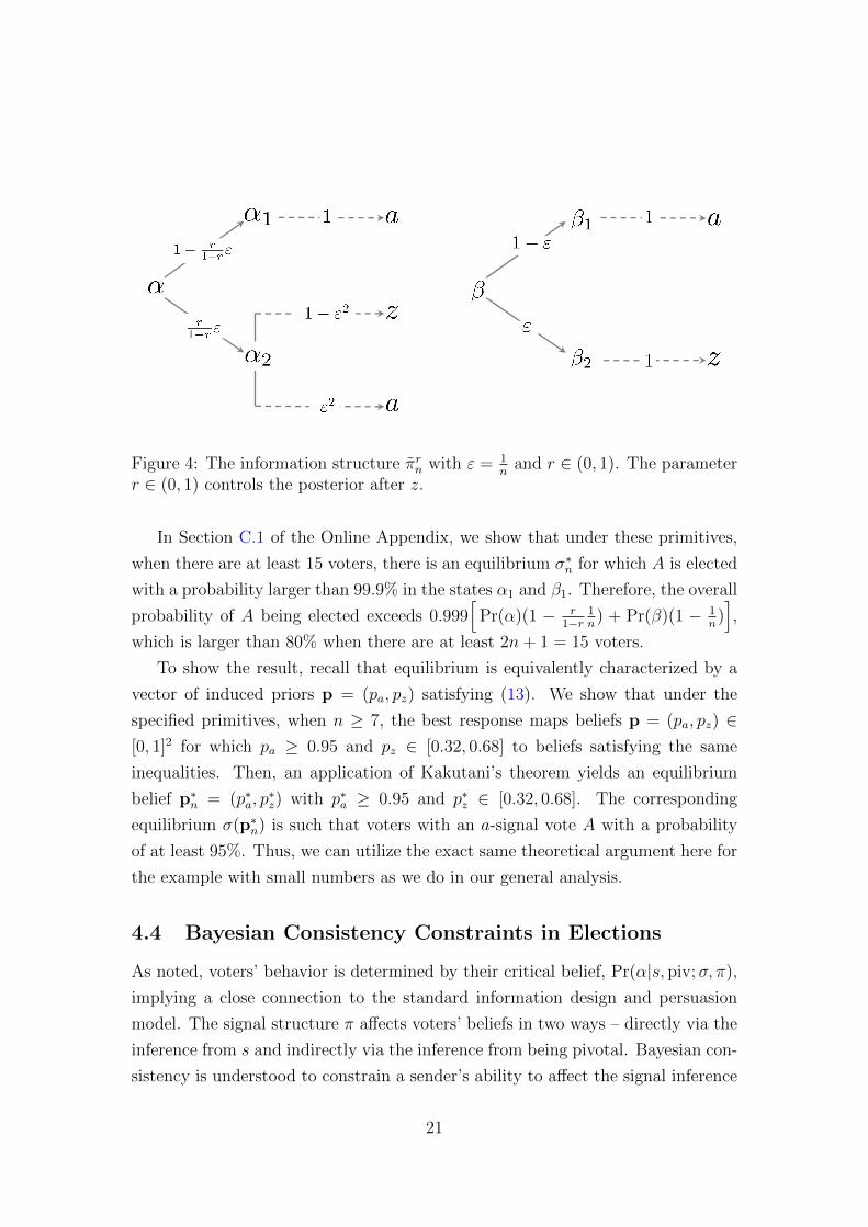
Figure 4: The information structure πrn with ε = 1n
and r ∈ (0, 1). The parameterr ∈ (0, 1) controls the posterior after z.
In Section C.1 of the Online Appendix, we show that under these primitives,
when there are at least 15 voters, there is an equilibrium σ∗n for which A is elected
with a probability larger than 99.9% in the states α1 and β1. Therefore, the overall
probability of A being elected exceeds 0.999[
Pr(α)(1 − r1−r
1n) + Pr(β)(1 − 1
n)],
which is larger than 80% when there are at least 2n+ 1 = 15 voters.
To show the result, recall that equilibrium is equivalently characterized by a
vector of induced priors p = (pa, pz) satisfying (13). We show that under the
specified primitives, when n ≥ 7, the best response maps beliefs p = (pa, pz) ∈[0, 1]2 for which pa ≥ 0.95 and pz ∈ [0.32, 0.68] to beliefs satisfying the same
inequalities. Then, an application of Kakutani’s theorem yields an equilibrium
belief p∗n = (p∗a, p∗z) with p∗a ≥ 0.95 and p∗z ∈ [0.32, 0.68]. The corresponding
equilibrium σ(p∗n) is such that voters with an a-signal vote A with a probability
of at least 95%. Thus, we can utilize the exact same theoretical argument here for
the example with small numbers as we do in our general analysis.
4.4 Bayesian Consistency Constraints in Elections
As noted, voters’ behavior is determined by their critical belief, Pr(α|s, piv;σ, π),
implying a close connection to the standard information design and persuasion
model. The signal structure π affects voters’ beliefs in two ways – directly via the
inference from s and indirectly via the inference from being pivotal. Bayesian con-
sistency is understood to constrain a sender’s ability to affect the signal inference
21
by choice of π; however, the indirect effect is much less constrained.
Bayesian consistency—or the law of iterated expectation—requires that
Pr(α) =∑s∈S
[Pr(s, piv)Pr(α|s, piv) + Pr(s,¬piv)Pr(α|s,¬piv)] , (41)
where Pr(α|s,¬piv; σ, π) is the posterior conditional on not being pivotal; we
omitted (σ, π). With a single voter, Pr(piv) = 1, and so the expected critical
belief is constrained to be the prior. However, with many voters, Pr(piv) becomes
small, and, consequently, (41) imposes only a small constraint.
The effectiveness of “pivotal persuasion” has been observed before in a setting
with known preferences and no private information by the voters; see our discus-
sion of the related literature in Section 7.2; especially Chan, Gupta, Li, and Wang
(2019) and Bardhi and Guo (2018).
Intuitively, what matters is that voters react to the closeness of the election.
The closeness of the election tells voters something about the information of others,
and, in this way, about the quality of the signal structure. The quality of the signal
structure, in turn, affects the meaning of the own information.
In our construction, one may interpret the signal structure πr as releasing
either a high quality signal—in substates {α1, β1}—or a low quality signal—in
substates {α2, β2}. The closeness of the election depends on the signal quality.
In particular, when the quality of the signal structure is high, all voters observe
the same revealing signal and the election is far from close. Conversely, when
the election is close, this is because the quality of the signal is low. In this case,
most voters learn that the signal quality is low but some may receive erroneous
messages. In particular, when the election is close and the signal quality is low,
the meaning of a b signal changes from being indicative of β to being an erroneous
signal indicative of α.
The pivotal voting model considers the extreme case in which voters react per-
fectly to the closeness of the election; it illustrates the effectiveness of persuasion
in this case. In Section 4.6.4, we discuss a model variant with some behavioral
types who do not condition on being pivotal.
4.5 Sketch of the Proof: General Policy
Now, we allow for non-monotone Φ and show that the sender can implement any
intended state-dependent policy, including the one that inverts the full-information
outcome.
22

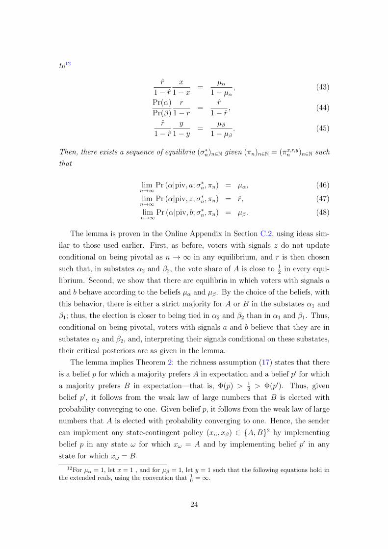
Figure 5: The information structure πx,r,yn with ε = 1n
and (x, r, y) ∈ [0, 1]3. Theparameter r controls the posterior after z and the parameters x and y control thebeliefs after a and b, respectively, conditional on being in substate α2 or β2.
For this, we consider the information structure depicted in Figure 5. The
signals are (almost) public, similar to the information structure in the previous
section from Figure 3. Moreover, as before, the signals a and b reveal the state
(almost) perfectly. The signal z contains only limited information since r ∈ (0, 1).
When observing the signal z, a voter knows that the substate must be either α2
or β2, and her belief conditional on signal z is given by
limn→∞
Pr(α|z; πx,r,yn )
Pr(β|z; πx,r,yn )= lim
n→∞
Pr(α|{α2, β2}; πx,r,yn )
Pr(β|{α2, β2}; πx,r,yn )=
Pr(α)
Pr(β)
r
1− r. (42)
We prove Theorem 2 by showing that by choosing the parameters (x, r, y) ∈[0, 1]3 appropriately, the sender can implement almost any belief µα in state α and
any belief µβ in state β as n → ∞, in the sense that, with probability close to
one, almost all voters will have such beliefs conditional on being pivotal.
Lemma 1 Let r solve Φ(r) = 12
and suppose r /∈ {0, 1}. Take any (µα, µβ) ∈[0, 1]2 with Φ(µα) 6= 1
2and Φ(µβ) 6= 1
2and choose (x, r, y) ∈ [0, 1]3 as the solutions
23
to12
r
1− rx
1− x=
µα1− µα
, (43)
Pr(α)
Pr(β)
r
1− r=
r
1− r, (44)
r
1− ry
1− y=
µβ1− µβ
. (45)
Then, there exists a sequence of equilibria (σ∗n)n∈N given (πn)n∈N = (πx,r,yn )n∈N such
that
limn→∞
Pr (α|piv, a;σ∗n, πn) = µα, (46)
limn→∞
Pr (α|piv, z;σ∗n, πn) = r, (47)
limn→∞
Pr (α|piv, b;σ∗n, πn) = µβ. (48)
The lemma is proven in the Online Appendix in Section C.2, using ideas sim-
ilar to those used earlier. First, as before, voters with signals z do not update
conditional on being pivotal as n → ∞ in any equilibrium, and r is then chosen
such that, in substates α2 and β2, the vote share of A is close to 12
in every equi-
librium. Second, we show that there are equilibria in which voters with signals a
and b behave according to the beliefs µα and µβ. By the choice of the beliefs, with
this behavior, there is either a strict majority for A or B in the substates α1 and
β1; thus, the election is closer to being tied in α2 and β2 than in α1 and β1. Thus,
conditional on being pivotal, voters with signals a and b believe that they are in
substates α2 and β2, and, interpreting their signals conditional on these substates,
their critical posteriors are as given in the lemma.
The lemma implies Theorem 2: the richness assumption (17) states that there
is a belief p for which a majority prefers A in expectation and a belief p′ for which
a majority prefers B in expectation—that is, Φ(p) > 12> Φ(p′). Thus, given
belief p′, it follows from the weak law of large numbers that B is elected with
probability converging to one. Given belief p, it follows from the weak law of large
numbers that A is elected with probability converging to one. Hence, the sender
can implement any state-contingent policy (xα, xβ) ∈ {A,B}2 by implementing
belief p in any state ω for which xω = A and by implementing belief p′ in any
state for which xω = B.
12For µα = 1, let x = 1 , and for µβ = 1, let y = 1 such that the following equations hold inthe extended reals, using the convention that 1
0 =∞.
24
4.6 Robustness
In this section, we discuss the robustness of the persuasion result in Theorem 2.
In particular, we ask: Can the sender be persuasive even if his commitment power
is limited? Can he be persuasive if he does not know the exact details of the
environment? How “stable” is the equilibrium? Are there other equilibria?
4.6.1 Persuasion with Partial Commitment
We relax the assumption that the sender can perfectly commit to an informa-
tion structure. To model partial commitment, we follow Lipnowski, Ravid, and
Shishkin (2019), Min (2017), and Frechette, Lizzeri, and Perego (2019). The
sender announces an information structure but is committed to the announced
information structure only with probability χ ∈ (0, 1); otherwise, he can freely
release any signal profile from its support.
Formally, we assume that, given some targeted state-dependent policy (x (α) , x (β)) ∈{A,B}2, the sender’s payoff is one if the targeted policy is implemented and zero
otherwise. An information structure π with signal set S, a no-commitment strat-
egy of the sender ψ∗ : {α, β} → ∆(S2n+1), and a voter strategy σ∗ form a χ-
equilibrium (Lipnowski, Ravid, and Shishkin, 2019) if ψ∗ is a best response by the
sender given that the voters follow the strategy σ∗ and σ∗ is a voting equilibrium
given that the sender commits to π with probability χ and otherwise sends signals
according to ψ∗.
Perhaps somewhat surprisingly, it turns out that the sender needs almost no
commitment power: He can persuade voters whenever n is large for any χ > 0,
no matter how small.
Proposition 1 Suppose that the sender is committed with some probability χ >
0. Then, for every preference distribution Φ, every prior Pr (α) ∈ (0, 1), and
every state-dependent policy (x (α) , x (β)) ∈ {A,B}2, there exists a sequence of
χ-equilibria (πn, ψ∗n, σ
∗n)n∈N, such that
limn→∞
Pr (x (α) |α; πn, ψ∗n, σ
∗n, n) = 1,
limn→∞
Pr (x (β) |β; πn, ψ∗n, σ
∗n, n) = 1.
The following discussion proves the proposition. We consider, first, the con-
stant target policy A, that is, x(α) = x(β) = A. As noted in Section 4.3, with
full commitment, this policy can be implemented by the information structure πrn
25
from Figure 4, which sends signal a with a probability of one in substates α1 and
β1. Given πrn with φ(r) = 12, there are voting equilibria σ∗n in which, following
signal a, the vote share of A is strictly larger than 1/2, whereas, after z, the vote
share is equal to 1/2. Now, take any χ ∈ (0, 1). Given the voting behavior σ∗n,
the best-response ψ∗ of the sender is to send signal a to all voters because signal
a leads to a higher vote share for A than signal z. Now, it turns out that, for
any χ > 0 and n large enough, there is a signal structure πχn such that πχn , χ,
and ψ∗ jointly imply the exact same distribution over signals as the original infor-
mation structure πrn.13 Hence, the original voting behavior σ∗n is a best response
to πχn and ψ∗. In other words, (πχn , ψ∗, σ∗n) form a χ-equilibrium that implements
x(α) = x(β) = A as n→∞.
The construction shows that one can find such πχn whenever χ > max ( 1n
r1−r ,
1n).
Thus, the required commitment power is vanishing at rate 1/n. The key observa-
tion is that πrn is already sending the sender’s preferred signal a to all voters with
probability close to 1 in both states.
Second, consider the targeted policy (x (α) , x (β)) = (B,A) that inverts the
full-information outcome. Let π(x,r,y)n be the information structure from Figure
5. By Lemma 1 and the subsequent discussion, there are parameters (x, r, y) and
equilibria σ∗n that implement the targeted policy. The voting behavior is such
that, after a, the vote share of A is strictly smaller than 1/2, after z it is equal to
1/2, and after b it is strictly larger than 1/2. Given this voting behavior and the
targeted policy, the sender’s best response ψ∗ is to send the signal a to all voters
when the state is α and b to all voters when the state is β (recall that a majority
of the voters are voting B with an a signal and A with a b signal). Finally, for
any χ > 0 and n large enough, one can construct a modified information structure
πχn in the same way as before such that πχn , χ, and ψ∗ jointly imply the same
signal distribution as π(x,r,y)n ; so, σ∗n is a best response, proving the existence of a
χ-equilibrium that implements (x (α) , x (β)) = (B,A).
Numerical Example (continued). Recall the example with Φ(p) = p and
13The sender’s information structure πχn is constructed as follows: in α, he sends the signal a to
all voters with probability (1− r(α)1−r(α)
1n ), where r(α) solves χ(1− r(α)
1−r(α)1n )+(1−χ) = 1− r
1−r1n ;
in β, he sends the signal a to all voters with probability (1 − r(β)1−r(β)
1n ), where r(β) solves
χ(1− r(β)1−r(β)
1n ) + (1−χ) = 1− 1
n . In α, otherwise, each voter receives a signal z randomly with
probability 1− 1n2 , and a signal a with probability 1
n2 ; in β, otherwise, all voters receive the public
signal z. This construction is feasible if χ > max ( 1n
r1−r ,
1n ), which ensures that (1 − r(α)
1−r(α)1n )
and (1− r(β)1−r(β)
1n ) are in (0, 1).
26
Pr(α) = 13. Given full commitment and the information structure πrn with r = 2
3,
when there are at least 2n+1 = 15 voters, there are equilibria σ(p∗n) such that the
constant policy A is elected with a probability larger than 80%. The construction
of σ(p∗n) shows that, following signal a, the vote share of A is strictly larger than
0.95, whereas, after z, the vote share is in [0.3, 0.7]. Therefore, the sender’s best
response to σ(p∗n) is to send the public signal a, i.e. ψ∗(α) = ψ∗(β) = (a, . . . , a).
Again, for any χ > 1n
r1−r = 3
n, there is a signal structure πχn such that πχn , χ, and ψ∗
jointly imply the exact same distribution over signals as the original information
structure πrn; so σ(p∗n) is a continuation equilibrium, proving the existence of a χn-
equilibrium where A is elected with a probability larger than 80% when 2n+1 ≥ 15
and χ > 3n.
4.6.2 Robustness: Detail-Freeness
In this section, we show that to persuade the voters, the signal structure does not
need to be finely tuned to the details of the environment. Suppose that the prior
and the preference distribution are such that
|Φ(0)− 1
2| > |Φ(Pr(α))− 1
2|, (49)
|Φ(1)− 1
2| > |Φ(Pr(α))− 1
2|; (50)
therefore, when the citizens vote optimally given their beliefs, the election is closer
to being tied when they are uninformed and hold the prior belief relative to when
they know the state.
Proposition 2 Take r = 1 and (x, y) ∈ {0, 1}2. For any prior and preference
distribution satisfying (49) and (50), there is a sequence of equilibria (σ∗n)n∈N given
the sequence of signal structures (πx,r,yn )n∈N such that
limn→∞
Pr (α|piv, a;σ∗n) = x, (51)
limn→∞
Pr (α|piv, z;σ∗n) = Pr(α), (52)
limn→∞
Pr (α|piv, b;σ∗n) = y. (53)
The proposition implies that the sender can implement any policy using a
single signal structure that works uniformly across the large set of priors and
preference distributions satisfying (49) and (50). For example, the constant policy
A is implemented by choosing x = y = 1, which leads to an equilibrium in which
27

A has a vote share Φ(1) as the election becomes large.
The proof is in the Online Appendix in Section C.3. The basic idea is that,
given this signal, the vote shares are close to Φ(Pr(α)) in states α2 and β2. Hence,
by assumptions (49) and (50), if voters behave according to the posteriors x and
y in states α1 and β1, the election is closer to being tied in α2 and β2 than
in α1 and β1. Thus, just as before, conditional on being pivotal, voters with
signals a and b believe that they are in states α2 and β2, and—interpreting their
signals conditional on these substates—their critical posteriors are as given in the
proposition.
A similar argument implies that the signal structure from Lemma 1 is also
effective when the actual environment is slightly different: When the prior and Φ
is slightly different from the one used to calculate (x, r, y), then there is still an
equilibrium close-by with critical beliefs that are close to µα, r, and µβ, provided
that vote shares at the critical beliefs imply that the election is still closer to being
tied in states α2 and β2 than in states α1 and β1.
Random Signal Quality. Note that the signal from Proposition 2 matches
the description in the introduction. In particular, we can swap the timing in
the description of the signal. Rather than choosing the “quality” of the signal
after the state of nature has realized, one can first choose randomly whether the
signal is “revealing” or “obfuscating” and then, if it is revealing, send a signal
corresponding to the realized state of nature to all voters (as in substates α1 and
β1), and, if it is obfuscating, send the signals z or b in α and z or a in β (as in
substates α2 and β2 when x = 0 and y = 1).
4.6.3 Robustness: Basin of Attraction
We show that, for a large set of initial strategies, an iterated best response leads
quickly to the “manipulated equilibrium” of Theorem 2 described earlier.
Let (µα, µβ) be any pair of beliefs with Φ(µα) 6= 12
and Φ(µβ) 6= 12. By Lemma
1, there is a sequence of information structures (πx,r,yn )n∈N and equilibria (σ∗n)n∈N
that implements the pair of beliefs as n→∞, in the sense that, with probability
close to 1, almost all voters will have such beliefs conditional on being pivotal.
Hence, by choosing (µα, µβ) appropriately, a sender can implement any desired
policy. The next result shows that, for almost any strategy σ, the twice-iterated
best response is arbitrarily close to σ∗n when n is large, in the sense that the
posteriors conditional on being tied are close to (µα, µβ).
28

First, let us define the twice-iterated best response: Take any belief p and the
strategy σp that is optimal given these beliefs. Then, σρ(σp) is the best response
to σp and is optimal given the beliefs
ρ1(p) = ρ(σp), (54)
where ρ(σp) is the vector of the posteriors conditional on the pivotal event and
the signals. In the same way, σρ(σρ1(p)) is the best response to σρ1(p) (so it is the
twice-iterated best response to σp) and is optimal given the beliefs
ρ2(p) = ρ(σρ1(p)). (55)
Proposition 3 shows that for almost any p, we have |ρ2 (p)−(µα, r, µβ) | < ε when n
is sufficiently large. This means that the twice-iterated best response is arbitrarily
close to the manipulated equilibrium σ∗n since the equilibrium is consistent with
the belief ρ(σ∗n) ≈ (µα, r, µβ); see (13).
Proposition 3 Take any beliefs (µα, µβ) ∈ [0, 1]2 with Φ(µα) 6= 12
and Φ(µβ) 6= 12
and the corresponding information structures (πx,r,yn )n∈N from Lemma 1.
For any δ > 0, there is some B ⊂ [0, 1]3 with Lebesgue-measure of at least 1−δand some n ∈ N such that, for all n ≥ n,
∀p ∈ B : |ρ2 (p)− (µα, r, µβ) | < δ. (56)
The proof is in Section C.4 in the Online Appendix. The proof also implies that,
for “almost any” strategy σ—even those that are not optimal given some belief
p—the twice-iterated best reply is arbitrarily close to the manipulated equilibrium
σ∗n when n is large, where the genericity requirement is with respect to the induced
vote shares and given by condition (100), replacing σp by σ.
Simple Reasoning. Proposition 3 illustrates that a simple reasoning un-
derlies the manipulated equilibrium σ∗n. The result loosely relates to the con-
cepts of level k-thinking and level-k-implementability (De Clippel, Saran, and
Serrano, 2019). The proposition implies that, for almost any strategy (a “behav-
ioral anchor”), the strategies that are consistent with level-2-thinking are close
to the manipulated equilibrium. In this sense, any state-dependent target policy
(x(α), x(β)) ∈ {A,B}2 is level-2-implementable.14
14De Clippel, Saran, and Serrano (2019) consider a different notion of level-2-implementability
29
4.6.4 Persuasion with Behavioral Types
The pivotal voting model considers the extreme case where voters react perfectly
to the closeness of the election when interpreting their information and illustrates
the effectiveness of persuasion in this case. The empirical literature has indeed
provided evidence for strategic voting behavior.15 However, while there is often a
significant fraction of the voters that are shown to act strategically, others behave
“sincerely”.16 We follow this literature—in particular the modeling in Kawai and
Watanabe (2013)—and consider an alternative model in which citizens have not
only a preference type but also a behavioral type. Each citizen is a “sincere voter”
with a probability κ ≥ 0, and, in that case, votes A only if ptα + (1 − p)tβ ≥ 0
for p = Pr(α|s; π), where s is her private signal and π the information structure.
Otherwise, with probability 1 − κ, a voter is a “pivotal voter” as in the analysis
before.
For concreteness, we discuss the effect of sincere voters in the setup of the
numerical example from Section 4.3 with Φ(p) = p, the information structure πrn
from Figure 4, and with Pr(α) = 13
and r = 23. Here, signal a contains almost no
information; therefore, the vote share of A among the sincere voters is roughly 13.
When n is large, this implies that the previous persuasion arguments continue to
work when κ13
+ (1−κ) > 12, which holds if κ < 3
4—roughly in line with estimates
from the empirical literature.17
The full analysis of a model with sincere voters may be worthwhile for future
research, especially when considering the implementation of the inverse of the full
information outcome, that is, x(α) = B and x(β) = A.
that demand that there is some behavioral anchor such that any profile of strategies that arelevel-1-consistent or level-2-consistent for this anchor implement a given social choice function.Here, almost any strategy can be such an anchor.
15See e.g. Guarnaschelli, McKelvey, and Palfrey (2000).16See e.g. Kawai and Watanabe (2013), who provide estimates of strrategic voters ranging
from 63.4% to 84.9%, or Esponda and Vespa (2014), who provide estimates between 20% and50%. There are also other behavioral models of voting, such as ethical voting (Feddersen andSandroni, 2006) or expressive voting that could be interesting as well.
17We revisit the example with sincere voters numerically in the Online Appendix in SectionF. Given the parameters Φ(p) = p and Pr(α) = 1
3 , suppose that the fraction of sincere voters isκ = 40%. Under these primitives, we show that when there are at least 170 voters, there is anequilibrium σ∗n for which A is elected with a probability larger than 99.9% in the states α1 andβ1.
30
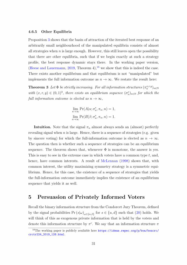
4.6.5 Other Equilibria
Proposition 3 shows that the basin of attraction of the iterated best response of an
arbitrarily small neighbourhood of the manipulated equilibria consists of almost
all strategies when n is large enough. However, this still leaves open the possibility
that there are other equilibria, such that if we begin exactly at such a strategy
profile, the best response dynamic stays there. In the working paper version,
(Heese and Lauermann, 2019, Theorem 4),18 we show that this is indeed the case.
There exists another equilibrium and that equilibrium is not “manipulated” but
implements the full information outcome as n→∞. We restate the result here:
Theorem 3 Let Φ be strictly increasing. For all information structures (πx,r,yn )n∈N
with (x, r, y) ∈ (0, 1)3, there exists an equilibrium sequence (σ∗n)n∈N for which the
full information outcome is elected as n→∞,
limn→∞
Pr(A|α;σ∗n, πn, n) = 1,
limn→∞
Pr(B|β;σ∗n, πn, n) = 1.
Intuition. Note that the signal πn almost always sends an (almost) perfectly
revealing signal when n is large. Hence, there is a sequence of strategies (e.g. given
by sincere voting) for which the full-information outcome is elected as n → ∞.
The question then is whether such a sequence of strategies can be an equilibrium
sequence. The theorem shows that, whenever Φ is monotone, the answer is yes.
This is easy to see in the extreme case in which voters have a common type t, and,
hence, have common interests. A result of McLennan (1998) shows that, with
common interest, the utility maximizing symmetry strategy is a symmetric equi-
librium. Hence, for this case, the existence of a sequence of strategies that yields
the full-information outcome immediately implies the existence of an equilibrium
sequence that yields it as well.
5 Persuasion of Privately Informed Voters
Recall the binary information structure from the Condorcet Jury Theorem, defined
by the signal probabilities Pr (s|ω)ω∈{α,β} for s ∈ {u, d} such that (20) holds. We
will think of this as exogenous private information that is held by the voters and
denote this information structure by πc. We say that an information structure π
18The working paper is publicly available here https://ideas.repec.org/p/bon/boncrc/
crctr224_2019_128.html.
31
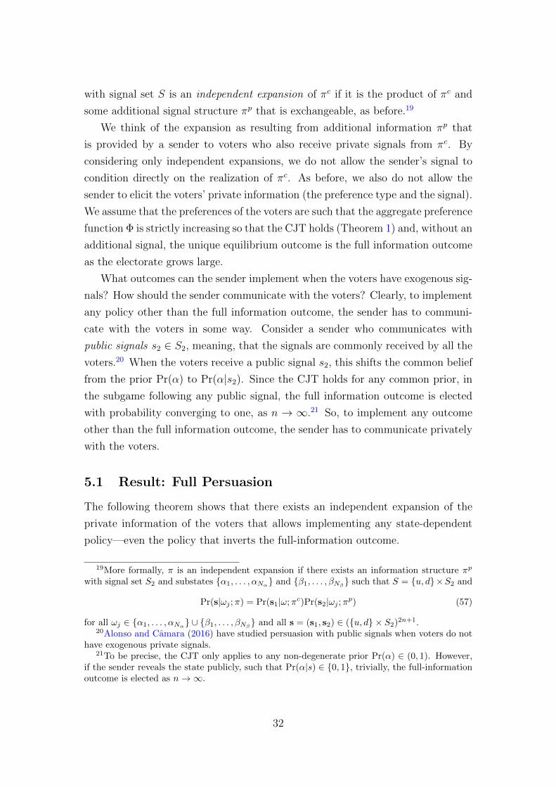
with signal set S is an independent expansion of πc if it is the product of πc and
some additional signal structure πp that is exchangeable, as before.19
We think of the expansion as resulting from additional information πp that
is provided by a sender to voters who also receive private signals from πc. By
considering only independent expansions, we do not allow the sender’s signal to
condition directly on the realization of πc. As before, we also do not allow the
sender to elicit the voters’ private information (the preference type and the signal).
We assume that the preferences of the voters are such that the aggregate preference
function Φ is strictly increasing so that the CJT holds (Theorem 1) and, without an
additional signal, the unique equilibrium outcome is the full information outcome
as the electorate grows large.
What outcomes can the sender implement when the voters have exogenous sig-
nals? How should the sender communicate with the voters? Clearly, to implement
any policy other than the full information outcome, the sender has to communi-
cate with the voters in some way. Consider a sender who communicates with
public signals s2 ∈ S2, meaning, that the signals are commonly received by all the
voters.20 When the voters receive a public signal s2, this shifts the common belief
from the prior Pr(α) to Pr(α|s2). Since the CJT holds for any common prior, in
the subgame following any public signal, the full information outcome is elected
with probability converging to one, as n → ∞.21 So, to implement any outcome
other than the full information outcome, the sender has to communicate privately
with the voters.
5.1 Result: Full Persuasion
The following theorem shows that there exists an independent expansion of the
private information of the voters that allows implementing any state-dependent
policy—even the policy that inverts the full-information outcome.
19More formally, π is an independent expansion if there exists an information structure πp
with signal set S2 and substates {α1, . . . , αNα} and {β1, . . . , βNβ} such that S = {u, d}×S2 and
Pr(s|ωj ;π) = Pr(s1|ω;πc)Pr(s2|ωj ;πp) (57)
for all ωj ∈ {α1, . . . , αNα} ∪ {β1, . . . , βNβ} and all s = (s1, s2) ∈ ({u, d} × S2)2n+1.20Alonso and Camara (2016) have studied persuasion with public signals when voters do not
have exogenous private signals.21To be precise, the CJT only applies to any non-degenerate prior Pr(α) ∈ (0, 1). However,
if the sender reveals the state publicly, such that Pr(α|s) ∈ {0, 1}, trivially, the full-informationoutcome is elected as n→∞.
32
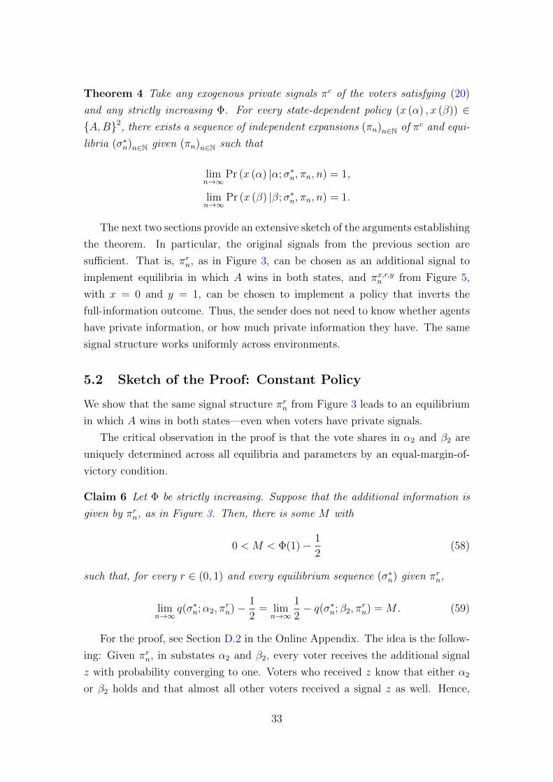
Theorem 4 Take any exogenous private signals πc of the voters satisfying (20)
and any strictly increasing Φ. For every state-dependent policy (x (α) , x (β)) ∈{A,B}2, there exists a sequence of independent expansions (πn)n∈N of πc and equi-
libria (σ∗n)n∈N given (πn)n∈N such that
limn→∞
Pr (x (α) |α;σ∗n, πn, n) = 1,
limn→∞
Pr (x (β) |β;σ∗n, πn, n) = 1.
The next two sections provide an extensive sketch of the arguments establishing
the theorem. In particular, the original signals from the previous section are
sufficient. That is, πrn, as in Figure 3, can be chosen as an additional signal to
implement equilibria in which A wins in both states, and πx,r,yn from Figure 5,
with x = 0 and y = 1, can be chosen to implement a policy that inverts the
full-information outcome. Thus, the sender does not need to know whether agents
have private information, or how much private information they have. The same
signal structure works uniformly across environments.
5.2 Sketch of the Proof: Constant Policy
We show that the same signal structure πrn from Figure 3 leads to an equilibrium
in which A wins in both states—even when voters have private signals.
The critical observation in the proof is that the vote shares in α2 and β2 are
uniquely determined across all equilibria and parameters by an equal-margin-of-
victory condition.
Claim 6 Let Φ be strictly increasing. Suppose that the additional information is
given by πrn, as in Figure 3. Then, there is some M with
0 < M < Φ(1)− 1
2(58)
such that, for every r ∈ (0, 1) and every equilibrium sequence (σ∗n) given πrn,
limn→∞
q(σ∗n;α2, πrn)− 1
2= lim
n→∞
1
2− q(σ∗n; β2, π
rn) = M . (59)
For the proof, see Section D.2 in the Online Appendix. The idea is the follow-
ing: Given πrn, in substates α2 and β2, every voter receives the additional signal
z with probability converging to one. Voters who received z know that either α2
or β2 holds and that almost all other voters received a signal z as well. Hence,
33

from their perspective, it is close to common knowledge that the game is close to
a game with a binary state and binary signals πc, as in the original setting of the
CJT. Recall that the proof of the CJT showed that the election must be equally
close to being tied in expectation; see (22). The same arguments implies (59) here.
Now, one can show that there is a sequence of equilibria in which the vote
share of A in state β1 approaches its maximum, Φ(1), and thus
limn→∞
q(σ∗n; β1, πn)− 1
2= Φ(1)− 1
2. (60)
Comparing (59) and (60), in this equilibrium sequence, the election is closer
to being tied in α2 than in β1. Hence, it follows from Claim 2 that
limn→∞
Pr (piv|β1;σ∗n)
Pr (piv|α2;σ∗n)= 0. (61)
Moreover, it also follows from Claim 2 that the inference from the pivotal event
dominates the direct inference from the signal.22 So, a voter with additional signal
s2 = b becomes convinced that the state is α2 for either realization of the private
signal s1 ∈ {u, d},limn→∞
Pr (α|piv, s1, s2 = b;σ∗n) = 1. (62)
Since all voters observe the additional signal s2 = b in state β1, it follows that
the vote share converges to Φ(1), as claimed in (60). Finally, it is clear that
such an equilibrium sequence leads to outcome A in both states with probability
converging to one.
Note that the basic idea here is similar to the one in Section 4.2 without the
private signal. Here, Claim 6 pins down behavior in states α2 and β2, analogously
to the implication of the previous Claim 3. Then, there is an equilibrium in which
A receives a strict majority in β1. In both settings, the equilibrium is supported
by the fact that the election is closer to being tied in α2 than in β1, so that,
conditional on being pivotal, voters with signal b become convinced that the state
is α2.
5.3 Sketch of the Proof: General Policy
The signal πx,r,yn from Figure 5 can again be used to implement any intended
policy by the appropriate choice of (x, r, y) ∈ [0, 1]3. The proof of this general
22See the proof of the analogous Claim 4.
34
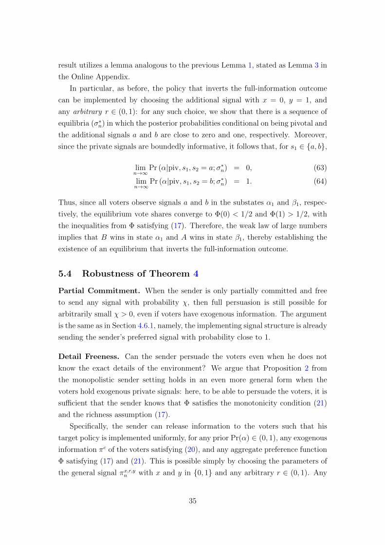
result utilizes a lemma analogous to the previous Lemma 1, stated as Lemma 3 in
the Online Appendix.
In particular, as before, the policy that inverts the full-information outcome
can be implemented by choosing the additional signal with x = 0, y = 1, and
any arbitrary r ∈ (0, 1): for any such choice, we show that there is a sequence of
equilibria (σ∗n) in which the posterior probabilities conditional on being pivotal and
the additional signals a and b are close to zero and one, respectively. Moreover,
since the private signals are boundedly informative, it follows that, for s1 ∈ {a, b},
limn→∞
Pr (α|piv, s1, s2 = a;σ∗n) = 0, (63)
limn→∞
Pr (α|piv, s1, s2 = b;σ∗n) = 1. (64)
Thus, since all voters observe signals a and b in the substates α1 and β1, respec-
tively, the equilibrium vote shares converge to Φ(0) < 1/2 and Φ(1) > 1/2, with
the inequalities from Φ satisfying (17). Therefore, the weak law of large numbers
implies that B wins in state α1 and A wins in state β1, thereby establishing the
existence of an equilibrium that inverts the full-information outcome.
5.4 Robustness of Theorem 4
Partial Commitment. When the sender is only partially committed and free
to send any signal with probability χ, then full persuasion is still possible for
arbitrarily small χ > 0, even if voters have exogenous information. The argument
is the same as in Section 4.6.1, namely, the implementing signal structure is already
sending the sender’s preferred signal with probability close to 1.
Detail Freeness. Can the sender persuade the voters even when he does not
know the exact details of the environment? We argue that Proposition 2 from
the monopolistic sender setting holds in an even more general form when the
voters hold exogenous private signals: here, to be able to persuade the voters, it is
sufficient that the sender knows that Φ satisfies the monotonicity condition (21)
and the richness assumption (17).
Specifically, the sender can release information to the voters such that his
target policy is implemented uniformly, for any prior Pr(α) ∈ (0, 1), any exogenous
information πc of the voters satisfying (20), and any aggregate preference function
Φ satisfying (17) and (21). This is possible simply by choosing the parameters of
the general signal πx,r,yn with x and y in {0, 1} and any arbitrary r ∈ (0, 1). Any
35

such information structure implements a targeted policy uniformly as outlined
before.
In a sense, the conditions for uniform implementability are weaker here than in
Proposition 2 in which we also required a condition on the prior. This is perhaps
surprising if one thinks of the voters’ exogenous information as a constraint on
the sender. The reason it holds is that, with exogenous private information, the
relevant “induced prior” after signal z, i.e., Pr(α|piv, z), adjusts endogenously to
ensure the equal-margin condition.
Belief Implementation. As in the monopolistic sender scenario, we provide a
result more general than Theorem 4: In the spirit of the literature on Bayesian
persuasion, we show that, for large electorates, there is a set of “implementable”
posterior belief distributions, including arbitrarily extreme beliefs. This result is
stated in Lemma 3 in the Online Appendix, and corresponds to Lemma 1 for the
monopolistic sender. However, when voters have exogenous information, not all
beliefs are implementable; this is consequential when the sender is only partially
informed, as discussed in Section 7.1.
Basin of Attraction. The results from Section 4.6.3 regarding the basin of
attraction of the manipulated equilibria for the case of a monopolistic sender do
not extend when voters have exogenous private information.23
Other Equilibria. We conjecture that there always also exists a sequence of
equilibria yielding the full-information outcome, as in the case of the monopolistic
sender (see Theorem 3). However, so far, we have not been able to prove this
result for the case with private signals.
6 Media Markets: An Application
We provide a stylized application to media markets. This serves two purposes:
first, we show that the main results of the paper can also be obtained in a setting
with normally distributed voter information. Second, within the application, we
can discuss concrete strategies of information manipulation.
23Instead, one can show the following: Let the sender release the information (πx,r,yn )n∈N to thevoters as in Lemma 3. When the electorate is large enough, for almost any initial strategy, underthe iterated best response, the voter behavior after signal z jumps back and forth indefinitelyfrom voting approximately according to σp, with p = Pr(α|s)s∈{a,z,b}, to voting approximatelyas if one of the states is known to be the true state. We omit the proof.
36

6.1 Benchmark: Exogenous Media
A media firm sends a message m = θ in α and m = −θ in β for some θ > 0. Voters
perceive the message with noise. That is, each voter receives a private signal
s = m + ε, where ε is drawn independently from a standard normal distribution;
see Figure 6.24 Each individual voter thus only holds partial information about the
state. Since the private signals s satisfy the monotone likelihood ratio property, a
higher signal leads to a higher belief in the likelihood of α.
For concreteness, suppose that voters have a common preference type: All
voters prefer A in α and B in β. They receive a payoff of tα = 1 if A is elected in
α and a payoff of tβ = −1 if A is elected in β; payoffs are normalized to zero if B
is elected. Hence, voters prefer the policy that matches the state they believe to
be more likely.
When there are 2n+ 1 voters, equilibrium can be described by a cutoff signal
s∗n that makes the voters indifferent: all voters with a signal s > s∗n assign a higher
probability to α than β and vote A and voters with a signal s < s∗n assign a higher
probability to β than α and vote B. One can show that s∗n → 0 as n→∞, for all
priors. Figure 6 illustrates the limit equilibrium. For the cutoff zero, a majority
of citizens votes A in α (shaded area) and B in β. For general preference distribu-
Figure 6: The density of the voters’ private signals in states α and β. The shadedare shows the share of citizens voting A when n is large.
tions, in this benchmark, all equilibrium sequences aggregate information perfectly
when preferences are monotone (that is, Φ is strictly increasing). This follows from
arguments similar to the ones used for Theorem 1; see also Bhattacharya (2013).
24Gaussian information is a common way to model that voters have noisy perceptions ofpolitical statements or states; see, e.g., the literature on electoral competition (Matejka andTabellini, 2016) or on media markets (Galperti and Trevino, 2018; Chen and Suen, 2019).
37
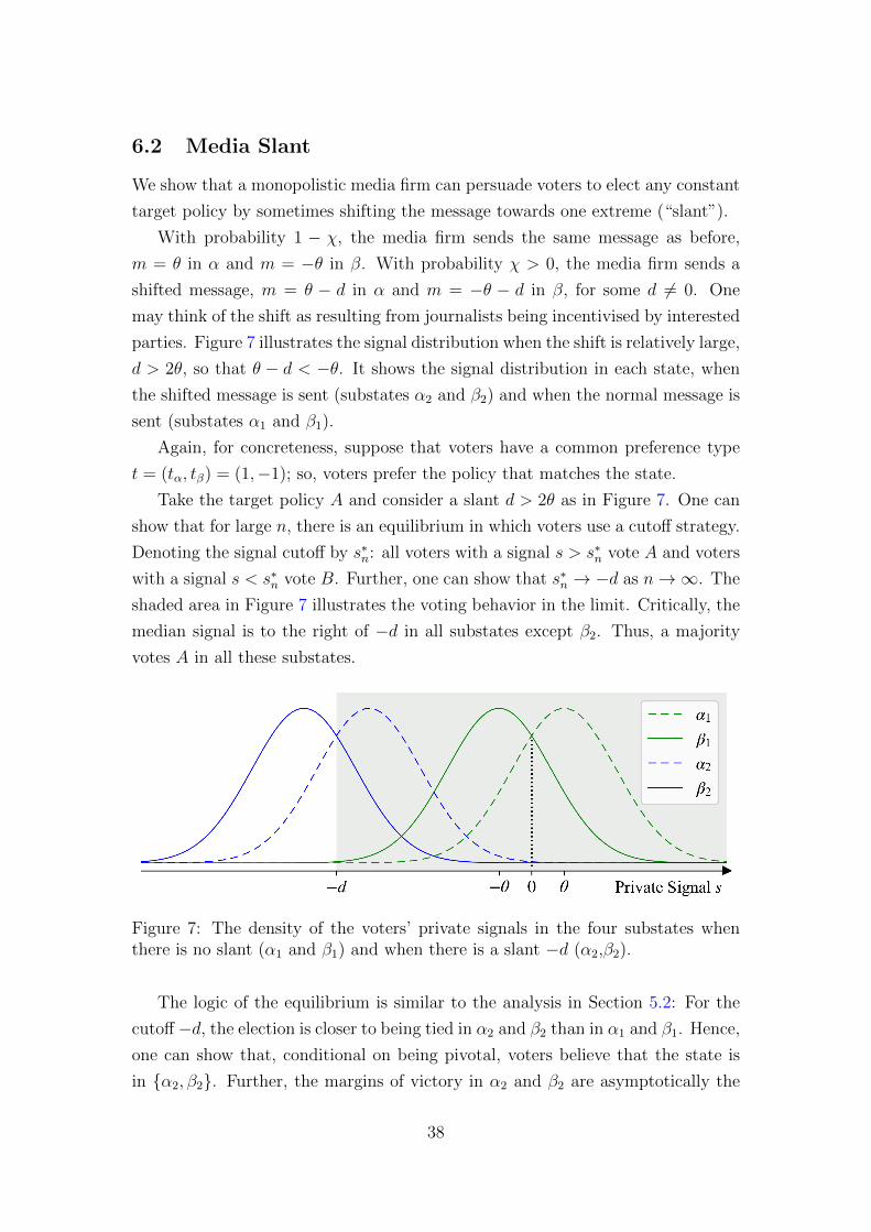
6.2 Media Slant
We show that a monopolistic media firm can persuade voters to elect any constant
target policy by sometimes shifting the message towards one extreme (“slant”).
With probability 1 − χ, the media firm sends the same message as before,
m = θ in α and m = −θ in β. With probability χ > 0, the media firm sends a
shifted message, m = θ − d in α and m = −θ − d in β, for some d 6= 0. One
may think of the shift as resulting from journalists being incentivised by interested
parties. Figure 7 illustrates the signal distribution when the shift is relatively large,
d > 2θ, so that θ − d < −θ. It shows the signal distribution in each state, when
the shifted message is sent (substates α2 and β2) and when the normal message is
sent (substates α1 and β1).
Again, for concreteness, suppose that voters have a common preference type
t = (tα, tβ) = (1,−1); so, voters prefer the policy that matches the state.
Take the target policy A and consider a slant d > 2θ as in Figure 7. One can
show that for large n, there is an equilibrium in which voters use a cutoff strategy.
Denoting the signal cutoff by s∗n: all voters with a signal s > s∗n vote A and voters
with a signal s < s∗n vote B. Further, one can show that s∗n → −d as n→∞. The
shaded area in Figure 7 illustrates the voting behavior in the limit. Critically, the
median signal is to the right of −d in all substates except β2. Thus, a majority
votes A in all these substates.
Figure 7: The density of the voters’ private signals in the four substates whenthere is no slant (α1 and β1) and when there is a slant −d (α2,β2).
The logic of the equilibrium is similar to the analysis in Section 5.2: For the
cutoff −d, the election is closer to being tied in α2 and β2 than in α1 and β1. Hence,
one can show that, conditional on being pivotal, voters believe that the state is
in {α2, β2}. Further, the margins of victory in α2 and β2 are asymptotically the
38
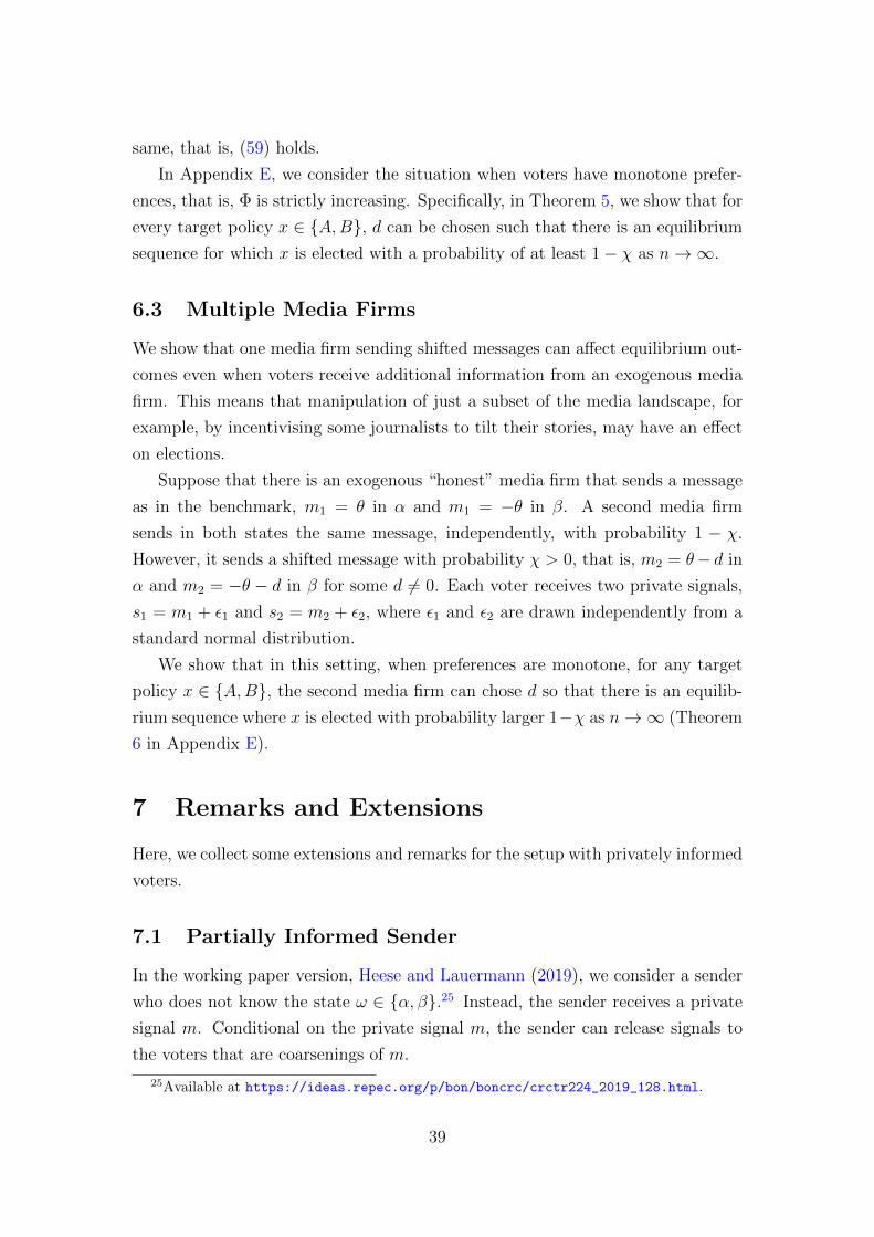
same, that is, (59) holds.
In Appendix E, we consider the situation when voters have monotone prefer-
ences, that is, Φ is strictly increasing. Specifically, in Theorem 5, we show that for
every target policy x ∈ {A,B}, d can be chosen such that there is an equilibrium
sequence for which x is elected with a probability of at least 1− χ as n→∞.
6.3 Multiple Media Firms
We show that one media firm sending shifted messages can affect equilibrium out-
comes even when voters receive additional information from an exogenous media
firm. This means that manipulation of just a subset of the media landscape, for
example, by incentivising some journalists to tilt their stories, may have an effect
on elections.
Suppose that there is an exogenous “honest” media firm that sends a message
as in the benchmark, m1 = θ in α and m1 = −θ in β. A second media firm
sends in both states the same message, independently, with probability 1 − χ.
However, it sends a shifted message with probability χ > 0, that is, m2 = θ− d in
α and m2 = −θ − d in β for some d 6= 0. Each voter receives two private signals,
s1 = m1 + ε1 and s2 = m2 + ε2, where ε1 and ε2 are drawn independently from a
standard normal distribution.
We show that in this setting, when preferences are monotone, for any target
policy x ∈ {A,B}, the second media firm can chose d so that there is an equilib-
rium sequence where x is elected with probability larger 1−χ as n→∞ (Theorem
6 in Appendix E).
7 Remarks and Extensions
Here, we collect some extensions and remarks for the setup with privately informed
voters.
7.1 Partially Informed Sender
In the working paper version, Heese and Lauermann (2019), we consider a sender
who does not know the state ω ∈ {α, β}.25 Instead, the sender receives a private
signal m. Conditional on the private signal m, the sender can release signals to
the voters that are coarsenings of m.
25Available at https://ideas.repec.org/p/bon/boncrc/crctr224_2019_128.html.
39
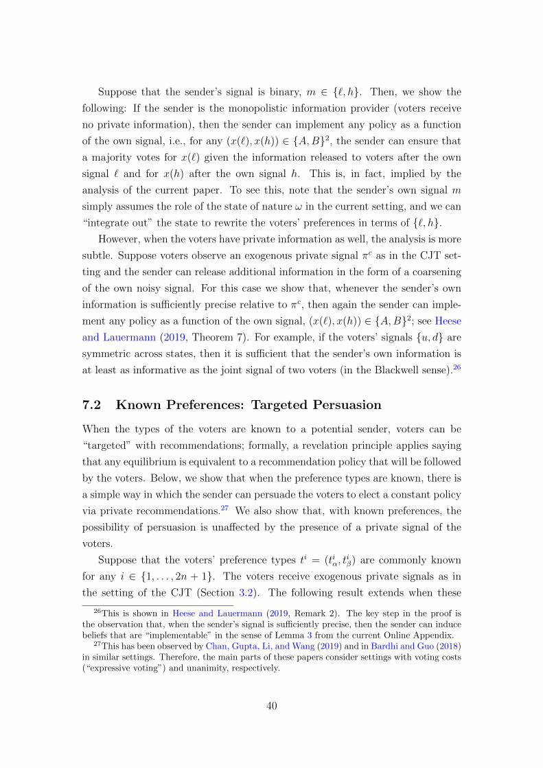
Suppose that the sender’s signal is binary, m ∈ {`, h}. Then, we show the
following: If the sender is the monopolistic information provider (voters receive
no private information), then the sender can implement any policy as a function
of the own signal, i.e., for any (x(`), x(h)) ∈ {A,B}2, the sender can ensure that
a majority votes for x(`) given the information released to voters after the own
signal ` and for x(h) after the own signal h. This is, in fact, implied by the
analysis of the current paper. To see this, note that the sender’s own signal m
simply assumes the role of the state of nature ω in the current setting, and we can
“integrate out” the state to rewrite the voters’ preferences in terms of {`, h}.However, when the voters have private information as well, the analysis is more
subtle. Suppose voters observe an exogenous private signal πc as in the CJT set-
ting and the sender can release additional information in the form of a coarsening
of the own noisy signal. For this case we show that, whenever the sender’s own
information is sufficiently precise relative to πc, then again the sender can imple-
ment any policy as a function of the own signal, (x(`), x(h)) ∈ {A,B}2; see Heese
and Lauermann (2019, Theorem 7). For example, if the voters’ signals {u, d} are
symmetric across states, then it is sufficient that the sender’s own information is
at least as informative as the joint signal of two voters (in the Blackwell sense).26
7.2 Known Preferences: Targeted Persuasion
When the types of the voters are known to a potential sender, voters can be
“targeted” with recommendations; formally, a revelation principle applies saying
that any equilibrium is equivalent to a recommendation policy that will be followed
by the voters. Below, we show that when the preference types are known, there is
a simple way in which the sender can persuade the voters to elect a constant policy
via private recommendations.27 We also show that, with known preferences, the
possibility of persuasion is unaffected by the presence of a private signal of the
voters.
Suppose that the voters’ preference types ti = (tiα, tiβ) are commonly known
for any i ∈ {1, . . . , 2n + 1}. The voters receive exogenous private signals as in
the setting of the CJT (Section 3.2). The following result extends when these
26This is shown in Heese and Lauermann (2019, Remark 2). The key step in the proof isthe observation that, when the sender’s signal is sufficiently precise, then the sender can inducebeliefs that are “implementable” in the sense of Lemma 3 from the current Online Appendix.
27This has been observed by Chan, Gupta, Li, and Wang (2019) and in Bardhi and Guo (2018)in similar settings. Therefore, the main parts of these papers consider settings with voting costs(“expressive voting”) and unanimity, respectively.
40
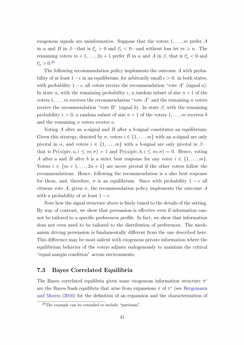
exogenous signals are uninformative. Suppose that the voters 1, . . . ,m prefer A
in α and B in β—that is tiα > 0 and tiβ < 0—and without loss let m > n. The
remaining voters m + 1, . . . , 2n + 1 prefer B in α and A in β, that is tiα < 0 and
tiβ > 0.28
The following recommendation policy implements the outcome A with proba-
bility of at least 1− ε in an equilibrium, for arbitrarily small ε > 0: in both states,
with probability 1− ε, all voters receive the recommendation “vote A” (signal a).
In state α, with the remaining probability ε, a random subset of size n+ 1 of the
voters 1, . . . ,m receives the recommendation “vote A” and the remaining n voters
receive the recommendation “vote B” (signal b). In state β, with the remaining
probability ε > 0, a random subset of size n + 1 of the voters 1, . . . ,m receives b
and the remaining n voters receive a.
Voting A after an a-signal and B after a b-signal constitutes an equilibrium:
Given this strategy, denoted by σ, voters i ∈ {1, . . . ,m} with an a-signal are only
pivotal in α, and voters i ∈ {1, . . . ,m} with a b-signal are only pivotal in β—
that is Pr(α|piv, a, i ≤ m;σ) = 1 and Pr(α|piv, b, i ≤ m;σ) = 0. Hence, voting
A after a and B after b is a strict best response for any voter i ∈ {1, . . . ,m}.Voters i ∈ {m + 1, . . . , 2n + 1} are never pivotal if the other voters follow the
recommendations. Hence, following the recommendation is a also best response
for them, and, therefore, σ is an equilibrium. Since with probability 1 − ε all
citizens vote A, given σ, the recommendation policy implements the outcome A
with a probability of at least 1− ε.Note how the signal structure above is finely tuned to the details of the setting.
By way of contrast, we show that persuasion is effective even if information can-
not be tailored to a specific preferences profile. In fact, we show that information
does not even need to be tailored to the distribution of preferences. The mech-
anism driving persuasion is fundamentally different from the one described here.
This difference may be most salient with exogenous private information where the
equilibrium behavior of the voters adjusts endogenously to maintain the critical
“equal-margin condition” across environments.
7.3 Bayes Correlated Equilibria
The Bayes correlated equilibria given some exogenous information structure πc
are the Bayes-Nash equilibria that arise from expansions π of πc (see Bergemann
and Morris (2016) for the definition of an expansion and the characterization of
28The example can be extended to include “partisans”.
41

Bayes correlated equilibria). In terms of Bayes correlated equilibria, Theorem 4
means that for any state-dependent outcome function (x (α) , x (β)) ∈ {A,B}2,
there exists a sequence of Bayes correlated equilibria given πc that leads to this
outcome as n→∞.
8 Related Literature
Voter Persuasion Literature. The paper is related to work on information
design in general (see Bergemann and Morris (2019) for a survey), especially with
multiple receivers (e.g., Mathevet, Perego, and Taneva (2020)).
Previous work on persuasion in an election context has studied persuasion in
settings in which the preferences of the voters are commonly known and voters have
no access to exogenous private signals. The previous work has considered public
signals by the sender (Alonso and Camara, 2016), persuasion with conditionally
independent private signals by the sender (Wang, 2013), and targeted persuasion
with private signals by the sender (Bardhi and Guo, 2018; Chan, Gupta, Li, and
Wang, 2019). We discussed persuasion when the preferences of the voters are
known in Section 7.2, and we showed how the persuasion mechanism and its logic
are quite different.
In contrast to the existing literature, we revisit the general voting setting
of Feddersen and Pesendorfer (1997) with private preferences: In this setup, as
a consequence of the Condorcet Jury Theorem, there is no scope for persuasion
with public signals and also no scope for persuasion with conditionally independent
private signals; see Theorem 1.
More generally, most of the Bayesian persuasion literature assumes that the
sender has extensive knowledge of the environment; in particular, perfect knowl-
edge about the state and receiver types is typically assumed.29 In this paper, the
informational requirements for persuasion are significantly weaker. We allow for
private preferences and exogenous private signals of the receivers; we also consider
the case in which the sender has incomplete information regarding the prior prob-
abilities of the state, the distribution of the private preference types of the voters,
or the distribution of the private signals of the voters (see Section 4.6.2 and Sec-
tion 5.4). In the working paper version, Heese and Lauermann (2019), we consider
the case in which the sender’s information regarding the state is incomplete (see
29Exceptions are Guo and Shmaya (2019) and Kolotilin, Mylovanov, Zapechelnyuk, and Li(2017), who study persuasion of a single, privately informed receiver.
42

Section 7.1). Further, we show that persuasion requires almost no commitment
power.
Several other papers study how groups can be influenced through strategic
information transmission, but are less closely related: For example, Kerman, Her-
ings, and Karos (2020) study targeted persuasion via private signals when the
sender is restricted to use signals that induce the voters to behave sincerely; com-
pare to the discussion of targeted persuasion in Section 7.2. Levy, Moreno de
Barreda, and Razin (2018) study persuasion of voters with correlation neglect.
Schipper and Woo (2019) study the persuasion of voters who are unaware of cer-
tain features. Schnakenberg (2015) studies a cheap talk setting in which an expert
tries to manipulate a voting body. Salcedo (2019) studies persuasion of subgroups
of receivers via private messages in a setting in which each receiver’s payoff de-
pends only on his own action and the state.
More distantly related is work on the design of an elicitation mechanism to ob-
tain information from multiple experts for an adversary to use (Gerardi, McLean,
and Postlewaite, 2009; Feng and Wu, 2019).
Information Aggregation Literature. Voting theory has identified several
circumstances in which information may fail to aggregate. We discuss the studies
that are most closely related: Feddersen and Pesendorfer (1997) (Section 6) show
that an invertibility problem causes a failure when there is aggregate uncertainty
with respect to the preference distribution conditional on the state. We have
already mentioned that Bhattacharya (2013) shows that information may fail to
aggregate when preference monotonicity is violated.
In a pure common-values setting, Mandler (2012) shows that a failure can oc-
cur when there is aggregate signal uncertainty conditional on the state. There is
a sense in which such aggregate uncertainty is necessary for a failure of informa-
tion aggregation, in the sense that if there is a single substate, the CJT applies
(Theorem 1 and the subsequent discussion). Here, as in his model, the voters’
updating about the signal distribution of others conditional on a close election
is important.30 Note that the pure common-values assumption implies that this
setting is a special case of a setting in which the individual voters’ preference type
is known (discussed in Section 7.2). In contrast to Mandler (2012), we consider a
setting in which voters do not have common values; rather than perturbing that
30Uncertainty regarding the signal distribution and updating about it is also central inAcharya and Meirowitz (2017), in which aggregate uncertainty supports sincere voting. Otherrecent contributions on the conditions for information aggregation are Kosterina (2019) andBarelli, Bhattacharya, and Siga (2019).
43

original signal, we study the effect of an additional signal in the canonical setting
by Feddersen and Pesendorfer (1997).
Additional related models, which show that elections perform poorly in ag-
gregating information are include Razin (2003), Acharya (2016), Ekmekci and
Lauermann (2019), Ali, Mihm, and Siga (2018) and Bhattacharya (2018).
9 Conclusion
In the canonical voting setting by Feddersen and Pesendorfer (1997), informa-
tion aggregation may be upset by an interested sender who provides additional
information to the voters. We have shown how an interested sender can exploit
strategic voters by manipulating their inference from the election being close. In
equilibrium, the closeness of the election tells voters something about the quality
of the information of the other voters, and, because signals are correlated, also
about the quality of their own signal. This way the sender can “steer” the meaning
of signals and make voters elect even the inverse of the full-information outcome.
What is particularly striking about the result is its robustness; almost no com-
mitment power of the sender is required. The resulting equilibrium is simple and
selected by an iterated best response dynamic. The sender does not need precise
knowledge of the environment (“detail-freeness”). In fact, the same information
structure that implements a given policy in the monopolistic sender setting also
implements the policy when voters have private information. Even a manipulator
with very limited knowledge about the state itself can persuade a large electorate.
We discuss concrete information strategies within an application to media mar-
kets. For example, we show that a media firm can persuade voters by broadcasting
news that is biased towards one extreme relative to the exogenous media.
Conceptually, our results also mean that equilibrium outcomes in the setting
by Feddersen and Pesendorfer (1997) can be hard to predict for an outside observer
without precise knowledge of the voters’ information. The outside observer must
be able to exclude the possibility that voters have access to additional information
of the form discussed here.
Information aggregation has also been studied in (double-) auctions, a setting
that shares some features with elections. An interesting question may be whether,
in auctions, information aggregation is an “informationally robust” prediction or
whether bidders having additional information can also upset it. Information
design in auction settings has been studied by Bergemann, Brooks, and Morris
44
(2016), Du (2018), and Yamashita et al. (2016), among others, but mostly with a
focus on revenue and efficiency.
The pivotal voting model considers the extreme case in which voters react
perfectly to the closeness of the election when interpreting their information and
illustrates the effectiveness of persuasion in this case. One may conjecture that,
in a setting in which voters react less sensitively, persuasion is still effective but,
presumably, less so. We provide some initial observations on this conjecture here.
Appendix
A Monopolistic Persuasion: Proof of Claim 3
Without loss of generality, suppose σn is such that q(α2 ;σn)(1 − q(α2 ;σn)) <
q(β2;σn)(1− q(β2;σn)) for all n. It follows directly from (7) that
limn→∞
Pr(piv|α2;σn, πn)
Pr(piv|β2;σn, πn)≤ 1. (65)
We now show that the reverse inequality also holds and thereby finish the proof of
the lemma. For this, we show the following. There exists some L > 0 and M > 0
such that, for all n and all σn satisfying the ordering above,
Pr(piv|α2;σn, πn)
Pr(piv|β2;σn, πn)≥(
1− L
Mn2
)n. (66)
First, it follows from (15) that the expected vote share for A in α2 differs from
the expected vote share for A in β2 maximally by the probability that b is observed
in α2, that is, by ε2 = 1n2 ; so,
|q(α2 ;σn)− q(β2 ;σn)| ≤ ε2, (67)
for all n. Second, recall that Φ(0) < q(ωj;σ) < Φ(1) for any strategy and any
substate ωj, and note that the derivative of h(q) = q(1 − q) is bounded by some
L > 0 on the compact interval [Φ(0),Φ(1)]. These observations taken together
imply that
h(q(β2 ;σn))∣∣∣h(q(α2 ;σn))
h(q(β2 ;σn)− 1∣∣∣ = |h(q(α2 ;σn))− h(q(β2 ;σn))| ≤ Lε2. (68)
45

for all n. Since 0 < Φ(0) < q(α2 ;σn) < Φ(1) and h is inverse U-shaped with
maximum at 12, this bound implies
h(q(α2 ;σn))
h(q(β2 ;σn)≥ 1− L
h(q(β2 ;σn))n2≥ 1− L
Mn2(69)
for M = min (h(Φ(0)), h(Φ(1))) and all n. Now, (66) follows from (7).
Finally, since limn→∞(1− LMn2 )n = 1, (66) implies that
limn→∞
Pr(piv|α2;σn, πn)
Pr(piv|β2;σn, πn)≥ 1. (70)
To see why limn→∞(1− LMn2 )n = 1, note that limn→∞(1− L
Mn2 )2n = limn→∞(1−√L√Mn
)2n(1+√L√Mn
)2n = e2√
LM e−2
√LM = e0 = 1 where we used limn→∞(1+ x
n)n = ex.
This finishes the proof of Claim 3.
References
Acharya, A. (2016): “Information aggregation failure in a model of social mo-bility,” Games and Economic Behavior, 100, 257–272.
Acharya, A., and A. Meirowitz (2017): “Sincere voting in large elections,”Games and Economic Behavior, 101, 121–131.
Ahn, D. S., and S. Oliveros (2012): “Combinatorial voting,” Econometrica,80(1), 89–141.
Ali, S. N., M. Mihm, and L. Siga (2018): “Adverse Selection in DistributivePolitics,” Working paper.
Alonso, R., and O. Camara (2016): “Persuading voters,” American EconomicReview, 106(11), 3590–3605.
Bardhi, A., and Y. Guo (2018): “Modes of persuasion toward unanimousconsent,” Theoretical Economics, 13(3), 1111–1149.
Barelli, P., S. Bhattacharya, and L. Siga (2019): “Full information equiv-alence in large elections,” Working paper.
Bergemann, D., B. A. Brooks, and S. Morris (2016): “Informationallyrobust optimal auction design,” Working paper.
Bergemann, D., and S. Morris (2016): “Bayes correlated equilibrium and thecomparison of information structures in games,” Theoretical Economics, 11(2),487–522.
46
(2019): “Information design: A unified perspective,” Journal of Eco-nomic Literature, 57(1), 44–95.
Bhattacharya, S. (2013): “Preference monotonicity and information aggrega-tion in elections,” Econometrica, 81(3), 1229–1247.
(2018): “Condorcet Jury theorem in a spatial model of elections,” Work-ing paper.
Chan, J., S. Gupta, F. Li, and Y. Wang (2019): “Pivotal persuasion,” Jour-nal of Economic Theory, 180, 178–202.
Chen, H., and W. Suen (2019): “Competition for Attention and News Quality,”working paper.
De Clippel, G., R. Saran, and R. Serrano (2019): “Level-Mechanism De-sign,” The Review of Economic Studies, 86(3), 1207–1227.
Du, S. (2018): “Robust mechanisms under common valuation,” Econometrica,86(5), 1569–1588.
Ekmekci, M., and S. Lauermann (2019): “Manipulated Electorates and In-formation Aggregation,” The Review of Economic Studies, Forthcoming.
Esponda, I., and E. Vespa (2014): “Hypothetical thinking and informationextraction in the laboratory,” American Economic Journal: Microeconomics,6(4), 180–202.
Feddersen, T., and W. Pesendorfer (1997): “Voting behavior and infor-mation aggregation in elections with private information,” Econometrica:, pp.1029–1058.
Feddersen, T., and A. Sandroni (2006): “A theory of participation in elec-tions,” American Economic Review, 96(4), 1271–1282.
Feng, T., and Q. Wu (2019): “Getting Information from Your Enemies,” Work-ing paper.
Frechette, G. R., A. Lizzeri, and J. Perego (2019): “Rules and commit-ment in communication,” Working paper.
Galperti, S., and I. Trevino (2018): “Shared Knowledge and Competitionfor Attention in Information Markets,” Working paper.
Gerardi, D., R. McLean, and A. Postlewaite (2009): “Aggregation ofexpert opinions,” Games and Economic Behavior, 65(2), 339–371.
Guarnaschelli, S., R. D. McKelvey, and T. R. Palfrey (2000): “Anexperimental study of jury decision rules,” American Political Science Review,94(2), 407–423.
47
Guo, Y., and E. Shmaya (2019): “The interval structure of optimal disclosure,”Econometrica, 87(2), 653–675.
Heese, C., and S. Lauermann (2019): “Persuasion and Information Aggre-gation in Large Elections,” CRC TR 224 discussion paper series, University ofBonn and University of Mannheim, Germany, https://ideas.repec.org/p/bon/boncrc/crctr224_2019_128.html.
Kamenica, E., and M. Gentzkow (2011): “Bayesian persuasion,” The Amer-ican Economic Review, 101(6), 2590–2615.
Kawai, K., and Y. Watanabe (2013): “Inferring strategic voting,” AmericanEconomic Review, 103(2), 624–62.
Kerman, T., P. Herings, and D. Karos (2020): “Persuading Strategic Vot-ers,” .
Kolotilin, A., T. Mylovanov, A. Zapechelnyuk, and M. Li (2017): “Per-suasion of a privately informed receiver,” Econometrica, 85(6), 1949–1964.
Kosterina, S. (2019): “Information Structures and Information Aggregation inElections,” Working paper.
Levy, G., I. Moreno de Barreda, and R. Razin (2018): “Persuasion withcorrelation neglect: media power via correlation of news content,” Workingpaper.
Lipnowski, E., D. Ravid, and D. Shishkin (2019): “Persuasion via weakinstitutions,” Working paper.
Mandler, M. (2012): “The fragility of information aggregation in large elec-tions,” Games and Economic Behavior, 74(1), 257–268.
Matejka, F., and G. Tabellini (2016): “Electoral competition with rationallyinattentive voters,” Journal of the European Economic Association.
Mathevet, L., J. Perego, and I. Taneva (2020): “On information design ingames,” Journal of Political Economy, 128(4), 1370–1404.
McLennan, A. (1998): “Consequences of the Condorcet jury theorem for ben-eficial information aggregation by rational agents,” American political sciencereview, 92(2), 413–418.
Min, D. (2017): “Bayesian persuasion under partial commitment,” Working pa-per.
Razin, R. (2003): “Signaling and election motivations in a voting model withcommon values and responsive candidates,” Econometrica, 71(4), 1083–1119.
Salcedo, B. (2019): “Persuading part of an audience,” Working paper.
48

Schipper, B., and H. Y. Woo (2019): “Political awareness and microtargetingof voters in electoral competition,” Quarterly Journal of Political Science, 14,41–88.
Schnakenberg, K. E. (2015): “Expert advice to a voting body,” Journal ofEconomic Theory, 160, 102–113.
Wang, Y. (2013): “Bayesian persuasion with multiple receivers,” Working paper.
Weinstein, J., and M. Yildiz (2007): “A structure theorem for rationalizabilitywith application to robust predictions of refinements,” Econometrica, 75(2),365–400.
Wilson, R. (1987): “Game-theoretic analyses of trading processes,” in Advancesin Economic Theory, Fifth World Congress, pp. 33–70.
Yamashita, T., et al. (2016): “Revenue Guarantee in Auction with a (Corre-lated) Common Prior and Additional Information,” Working paper.
49
Online Appendix
B Proof of the Condorcet Jury Theorem
Step 1 For all n and every equilibrium σ∗n, the vote share of A is larger in α than
in β,
0 < q(β;σ∗n, n) < q(α;σ∗n, n) < 1. (71)
This ordering of the vote shares follows from the likelihood ratio ordering of the
signals. In particular, recall the expression (8) for the posterior likelihood ratio of
two states conditional on a given voter’s signal s and the event that the voter is
pivotal,
Pr (α|s, piv;σ∗n, n)
1− Pr (α|s, piv;σ∗n, n)=
Pr (α)
Pr (β)
Pr (piv|α;σ∗n, n)
Pr (piv|β;σ∗n, n)
Pr(s|α; πc)
Pr(s|β; πc), (72)
where Pr (piv|β;σ∗n, n) > 0 because σ∗n is nondegenerate by (2). Therefore, Pr(u|α;πc)Pr(u|β;πc)
>Pr(d|α;πc)Pr(d|β;πc)
implies that Pr (α|u, piv;σ∗n, n) > Pr (α|d, piv;σ∗n, n). Now, (71) follows
from (15) and the monotonicity of Φ. Intuitively, the expected posterior in state
α is higher and this translates into a larger set of types preferring A given the
monotonicity of Φ.
Step 2 Voters cannot become certain of the state conditional on being pivotal,
that is, the inference from the pivotal event must remain bounded,
limn→∞
Pr (piv|α;σ∗n, n)
Pr (piv|β;σ∗n, n)∈ (0,∞) , (73)
for every convergent subsequence in the extended reals.
Suppose not and suppose instead, for example, that conditional on being pivotal,
voters become convinced that the state is β, i.e., η = limn→∞Pr(piv|α;σ∗n,n)Pr(piv|β;σ∗n,n)
= 0. This
would imply limn→∞ Pr (α|s, piv;σ∗n, n) = 0 for s ∈ {u, d}. Then, given Φ (0) < 12,
a strict majority would support B in both states. However, the election is then
closer to being tied in state α and voters would update toward state α conditional
on being pivotal, in contradiction to η = 0.
Formally, if η = 0 for some converging subsequence, then limn→∞ q(ω;σ∗n) =
Φ (0) < 12
for ω ∈ {α, β}. Therefore, for large enough n, (71) implies that
q(β;σ∗n) < q(α;σ∗n) < 1/2. Now, Claim 1 implies that voters update toward
state α, that is, Pr(piv|α;σ∗n,n)Pr(piv|β;σ∗n,n)
≥ 1, in contradiction to η = 0.
50

Step 3 In every equilibrium sequence (σ∗n)n∈N, the limit of the vote share of A is
larger in α than in β,
limn→∞
q(α;σ∗n) > limn→∞
q(β;σ∗n). (74)
From (73) and (72), we have that the limits of the posteriors conditional on being
pivotal and s ∈ {u, d} are interior and hence ordered,
0 < limn→∞
Pr (α|d, piv;σ∗n, n) < limn→∞
Pr (α|u, piv;σ∗n, n) < 1.
Now, (74) follows from (15) since Φ is strictly increasing.
Step 4 The election is equally close to being tied in expectation, that is, (22)
holds:
limn→∞
q(α;σ∗n)− 1
2= lim
n→∞
1
2− q(β;σ∗n).
Since voters must not become certain conditional on being pivotal by (73), Claim
2 requires that
limn→∞
∣∣∣∣q(α;σ∗n)− 1
2
∣∣∣∣ = limn→∞
∣∣∣∣q(β;σ∗n)− 1
2
∣∣∣∣ . (75)
Given the ordering of the limits of the vote shares from (74), the equation (75)
implies (22).
It follows from Step 4 and (74) that
limn→∞
q(α;σ∗n) >1
2> lim
n→∞q(β;σ∗n).
Therefore, by the weak law of large numbers, A wins in state α with probability
converging to 1 as n → ∞ and B wins in state β with probability converging to
1 as n→∞. This proves Theorem 1.
Sketch of the proof of Theorem 1’. To see why the theorem is true, note
that, given the binary state, the signals can be taken to be ordered by the mono-
tone likelihood ratio, without loss of generality. For any fixed information structure
π and any equilibrium σ∗n, it then follows from (72) that the distribution of poste-
riors Pr(α|piv, s;σ∗n, π, n) in the state α (as implied by the distribution over s) first
order stochastically dominates the distribution of posteriors Pr(α|piv, s;σ∗n, π, n)
in the state β. Then, given that Φ is monotone, it follows from (15) that the vote
shares satisfy the ordering (71). From (71) onward none of the arguments use that
the signals are binary.
51

By the same line of argument, Theorem 1 holds even when we allow the informa-
tion structure πn with a single substate to vary with n (keeping the signal set S
fixed), as long as the limit information structure is not completely uninformative.
C Monopolistic Persuasion
C.1 Numerical Example
Note that one example of a distribution G on [0, 1]× [−1, 0] that induces a uniform
distribution of ‘thresholds of doubt’, i.e. Φ with Φ(p) = p for all p ∈ [0, 1] is given
by the density31
g(tα, tβ) =
√
1 + (tβtα
)2−1
· (2 ·∫|tα|>|tβ |
√1 + (
tβtα
)2−1
dt)−1 if−tβtα−tβ
≤ 12,√
1 + ( tαtβ
)2−1
· (2 ·∫|tα|>|tβ |
√1 + (
tβtα
)2−1
dt)−1 if−tβtα−tβ
≥ 12.
We utilize the following auxiliary result.
Lemma 2 Consider any sequence of strategies (σn)n∈N and any sequence of in-
formation structures (πn)n∈N with a common set of substates across n. Then, for
any substates ωi, ω′j ∈ {α1, . . . , αNα} ∪ {β1, . . . , βNβ} and any n ∈ N,
Pr(piv|ωi;σn, πn)
Pr(piv|ω′j;σn, πn)=[1 +
(q(ω′j;σp)− 1
2)2 − (q(ωi;σ
p)− 12)2
14− (q(ω′j;σ
p)− 12)2
]n(76)
Proof. Let xn = q(ωi;σn)− 12
and yn = q(ω′j;σn)− 12. Then,
q(ωi;σn)(1− q(ωi;σn))
q(ω′j;σn)(1− q(ω′j;σn))=
(12
+ xn)(12− xn)
(12
+ yn)(12− yn)
=14− y2
n + y2n − x2
n14− y2
n
= 1 +y2n − x2
n14− y2
n
The claim follows from (8).
Fixed Point Argument.
31To see why, note that for each t >> 0, d(t) =[√
1 + ( tαtβ )2]
is the length of the indifference
plane of t. By setting the density of types proportional to 1d(t) , integrating over each indifference
plane gives the same number such that types are uniformly distributed across indifference planes.
52

Consider a belief p = (pa, pz) with
pa ≥ 0.95, (77)
pz ∈ [0.32, 0.68]. (78)
Consider the information structure πrn from Figure 4. Then, we have the following
bounds for n ≥ 7:
q(ω1;σp, n) ≥ 0.95 for ω1 ∈ {α1, β1}, (79)
q(α2;σp, n) > 0.3 (80)
q(β2;σp, n) ≤ 0.7. (81)
In the following, we omit the dependence on σp and on πn most of the time.
Step 1 For any n ∈ N and any ω1 ∈ {α1, β1}, ω′2 ∈ {α2, β2},
Pr(piv|ω′2)
Pr(piv|ω1)≥ (4.4)n (82)
Indeed,
Pr(piv|ω′2)
Pr(piv|ω1)
≥ [1 + minω1,ω′2
(q(ω1;σp)− 12)2 − (q(ω′2;σp)− 1
2)2
14− (q(ω1;σp)− 1
2)2
]n
≥ (1 + (( 9
20)2 − ( 4
20)2
14− ( 9
20)2
))
≥ (1 +65
19)n
≥ (4.42)n. (83)
where we used Lemma 2 for the inequality on the second line.
Step 2 For n ≥ 7: ρa(σp) ≥ 0.95, and ρz(σ
p) ∈ [0.32, 0.68].
First,
ρa(σp)
1− ρa(σp)≥ p0
1− p0
Pr(α2|α) Pr(b|α2) Pr(piv|α2)
Pr(β1|β) Pr(b|β1) Pr(piv|β1)
≥ 1
2
2n
1n2
(1− 1n)(4.42)n
≥ 82 for n ≥ 7.
53

where we used (83) for the inequality on the second line. Hence, for n ≥ 7,
ρ(σp)a ≥82
83> 0.95. (84)
Second,
Pr(piv|α2)
Pr(piv|β2)≤ [1 +
|(q(β2;σp)− 12)2 − (q(α2;σp)− 1
2)2|
14− (q(β2;σp)− 1
2)2
]n
≤ (1 +1n4 + 1
n2
14− 16
400
)n
≤ 2. for n ≥ 7.
where we used Lemma 2 for the inequality on the first line. For the inequality
on the second line, we used that z is sent with probability 1 − 1n2 in both α2
and β2 such that the difference in the squared margins of victory cannot exceed
(x+ 1n2 )2 − x2 ≤ 2x
n2 + 1n4 where x is the minimum margin of victory in the states
α2, β2. Finally, the inequality follows since the margin of victory in both α2 and
β2 is bounded by 0.2. So,
ρz(σp)z
1− ρz(σp)=
Pr(α)
Pr(β)
Pr(α2|α)
Pr(β2|β)
Pr(z|α2)
Pr(z|β2)
Pr(piv|α2)
Pr(piv|β2)
= (1− 1
n2)Pr(piv|α2)
Pr(piv|β2)
≤ 2 for n ≥ 7.
Consequently, for all n ≥ 7,
ρ(σp)z ≤2
3. (85)
Third,
Pr(piv|α2)
Pr(piv|β2)≥ (1−
|(q(β2;σp)− 12)2 − (q(α2;σp)− 1
2)2|
14− (q(β2;σp)− 1
2)2
≥ (1−1n4 + 1
n2
14− 16
400
)n
≥ 0.48 for n ≥ 7. (86)
54

So, for all n ≥ 7,
ρ(σp)z1− ρ(σp)z
= (1− 1
n2)Pr(piv|α2;σp)
Pr(piv|β2;σp)≥ 0.471.
This gives for all n ≥ 7,
ρ(σp)z ≥0.471
1 + 0.471≥ 0.32. (87)
The claim follows from (84), (85)), and (87).
Step 3 For n ≥ 7, there is an equilibrium σ∗n which satisfies (79) - (81).
It follows from Step 2 that, for any n ≥ 7, the continuous map that sends p to
ρ(σp) is a self-map on the set of beliefs that satisfy (77) - (78). It follows from the
Kakutani fixed point theorem that there exists fixed points p∗n that satisfy (77) -
(78). The corresponding strategies σp∗n are equilibria (compare to (13)) and they
satisfy (79) - (81).
Step 4 Given the equilibrium σ∗n for n ≥ 7, the probability that A is elected is
larger than 80%.
Evaluation of the binomial distribution shows that Pr(B(2n + 1, x)) > n) ≥0.999999 if n ≥ 7 and x ≥ 0.95. Hence, given σ∗n, A is elected with probabil-
ity larger than 99.9% in the states α1 and β1. Finally, the claim follows since the
probability of the substate being α1 or β1 is Pr(α)(1− r1−r
1n)+Pr(β)(1− 1
n), which
is larger than 0.8 when n ≥ 7, given that Pr(α) = 13
and r = 23. The fourth step
finishes the calculations for the example.
C.2 Proof of Lemma 1
C.2.1 Preliminaries: Voter Inference
The basic arguments of the previous discussion of the voters’ inference from Section
4.2.2 extend to the general case.
Consider the signal z and the inference about the relative likelihood of α2
and β2. As in Claim 3, for any strategy used by the other voters, the pivotal
event contains no information about the relative probability of α2 and β2 as the
electorate grows large.
55

Claim 7 Given any parameters (x, r, y) ∈ [0, 1]3 and any sequence of strategies
(σn)n∈N,
limn→∞
Pr(piv|α2;σn, πx,r,yn )
Pr(piv|β2;σn, πx,r,yn )
= 1. (88)
The arguments from the proof of the analogous Claim 3 hold verbatim with the
required changes in notation; therefore, the proof is omitted. Claim 7 and (42)
imply, in particular, that
limn→∞
Pr(α|z, piv;σn, πx,r,yn )
Pr(β|z, piv;σn, πx,r,yn )
=Pr(α)
Pr(β)
r
1− r. (89)
Next, we consider a signal s ∈ {a, b} and the voters’ inference about the relative
likelihood of α and β. We show that, analogous to Claim 4, for this signal, the
inference from the signal is dominated by the inference from being pivotal if the
election is closer to being tied in states α2 and β2 than in the states α1 and β1.
Claim 8 Take any sequence of strategies (σn)n∈N such that
limn→∞
maxω2∈{α2,β2}
|q(σn;ω2, πx,r,yn )− 1
2|
< limn→∞
minω1∈{α1,β1}
|q(σn;ω1, πx,r,yn )− 1
2|; (90)
then, for s ∈ {a, b},
limn→∞
Pr({α2, β2}|s, piv;σn, πx,r,yn )
Pr({α1, β1}|s, piv;σn, πx,r,yn )
=∞. (91)
The claim follows from the same arguments as Claim 4, and we omit this proof as
well.
For any sequence of strategies that satisfies (90), Claims 7 and 8 imply that,
for signal a,32
limn→∞
Pr(α|a, piv;σn, πx,r,yn )
Pr(β|a, piv;σn, πx,r,yn )
=Pr(α2|{α2, β2}, a;σn, π
x,r,yn )
Pr(β2|{α2, β2}, a;σn, πx,r,yn )
=Pr(α)
Pr(β)
r
1− rx
1− x(92)
32Recall the convention 10 = ∞, such that, for x = 1, the following equalities hold in the
extended reals.
56

and that for signal b,
limn→∞
Pr(α|b, piv;σn, πx,r,yn )
Pr(β|b, piv;σn, πx,r,yn )
=Pr(α2|{α2, β2}, b;σn, πx,r,yn )
Pr(β2|{α2, β2}, b;σn, πx,r,yn )
=Pr(α)
Pr(β)
r
1− ry
1− y. (93)
C.2.2 Implementable Beliefs
We use that an equilibrium is equivalently characterized by a vector of beliefs,
p∗ = (p∗a, p∗z, p∗b) such that p∗ = ρ
(σp∗); see (13). Take any δ > 0 and let
Bδ ={p ∈ [0, 1]3 | |p− (µα, r
′, µβ)| ≤ δ}
, (94)
so that Bδ is the set of beliefs at most δ away from (µα, r′, µβ).
We show that Claim 7 and 8 imply that there is a large set of belief triples
(µα, r′, µβ) such that, given σp, the posterior conditional on being pivotal is again
in Bδ, for any p ∈Bδ, any sufficiently small δ and any sufficiently large n.33
Claim 9 Let (µα, µβ) ∈ [0, 1]2 and r′ ∈ (0, 1) with
|Φ(µα)− 1
2| > |Φ(r′)− 1
2| and |Φ(µβ)− 1
2| > |Φ(r′)− 1
2|. (95)
For any δ > 0 small enough, there exists n(δ) such that for all n ≥ n(δ),
∀p ∈Bδ : ρ (σp; πx,r,yn , n) ∈ Bδ (96)
for (x, r, y) being the solutions to Pr(α)Pr(β)
r1−r
x1−x = µα
1−µα , Pr(α)Pr(β)
r1−r
y1−y =
µβµβ
, andPr(α)Pr(β)
r1−r = r′
1−r′ .
Proof. Let πn = πx,r,yn . Take any p ∈ Bδ and consider the corresponding strategy
σp. The condition (95) implies that for δ small enough, the election is closer to
being tied in the states α2 and β2 than in the states α1 and β1 in expectation as
n→∞:
∀p ∈Bδ: limn→∞
maxω2∈{α2,β2}
|q(ω2;σp, πn)− 1
2|
< limn→∞
minω1∈{α1,β1}
|q(ω1;σp, πn)− 1
2|. (97)
33In the following, we use the convention that dividing by zero yields a result of infinity such
that formulas like Pr(α)Pr(β)
r1−r
x1−x = µα
1−µα make sense for µα ∈ {0, 1}.
57
To see why, note that for n large enough, q(α2;σp, πn) ≈ Φ (pz) and q(β2;σp, πn) ≈Φ (pz) since almost all voters receive z in α2 and β2. Also, q(α1;σp, πn) = Φ (pa)
since all voters receive a in α1 and q(β1;σp, πn) = Φ (pb) since all voters receive
b in β1. In addition, by the continuity of Φ, for δ small enough, we have that
Φ (pz) ≈ Φ (r′), Φ (pa) ≈ Φ (µα) and Φ (pb) ≈ Φ (µβ). Finally, (97) follows then
from Φ (r) = 12
and Φ (µω) 6= 12
for ω ∈ {α, β}. Now, it follows from (97), Claim
8, and its implications (92) and (93) that
limn→∞
ρa (σp; πn, n) = µα, (98)
limn→∞
ρb (σp; πn, n) = µβ. (99)
for any δ > 0 small enough. Thus, the claim follows from (89), (98) and (99).
We finish the proof of Lemma 1. Let r = Pr(α)rPr(α)r+(1−Pr(α))(1−r) with Φ(r) = 1
2;
see (40). Take any (µα, µβ) with Φ(µα) 6= 12
and Φ(µβ) 6= 12. Then, given Claim
9, ρ(σp) is a self-map on Bδ for δ small enough and n ≥ n(δ). Since ρ(σp) is
continuous in p, it follows from Kakutani’s theorem that there exists a fixed point
p∗n ∈ Bδ for all n large enough, i.e., p∗n = ρ(σp∗n) and the corresponding behavior
σp∗n forms a sequence of equilibria. Lemma 1 follows from (98) and (99).
C.3 Proof of Proposition 2
We provide the proof for the constant target policyA in both states, i.e., (x(α), x(β)) =
(A,A). Let the sender use the information structures πn = πx,r,yn with x = y = 1
and r = 12. It follows from Claim 9 that, for any Φ for which (49) and (50) hold,
there is a δ small enough such that ρ(σp) is a self-map on Bδ = {p ∈ [0, 1]3 :
|p− (1,Pr(α), 1)| ≤ δ} for all n large enough.
Since ρ(σp) is continuous in p, it follows from Kakutani’s theorem that there
exists a fixed point p∗n ∈ Bδ for all n large enough, i.e., p∗n = ρ(σp∗n) and the
corresponding behavior σp∗n forms a sequence of equilibria that implements the
beliefs (µα, µβ) = (1, 1). Given (σp∗n)n∈N, the policy A wins in both states; this
follows since voters with an a and b-signal are supporting A with a probability
converging to Φ(1) > 12
and from the weak law of large numbers. The other cases
are analogous. This finishes the proof of the lemma.
58

C.4 Proof of Proposition 3 (Basin of Attraction)
Recall that for any strategy σ, the distance between the margin of victory in α2
and β2 is smaller than 2n2 in expectation since the probability that a voter receives
the signal z is at least 1 − 2n2 in both the substates. Now, consider any belief
p ∈ [0, 1]3 such that under the corresponding strategy σp the margins of victory
differ by at least δ > 0 for any other pair of substates. The theorem follows from
the following claim: we show that for any such belief p, the twice-iterated response
is δ-close to the manipulated equilibrium when n is large enough.
Claim 10 Take any beliefs (µα, µβ) ∈ [0, 1]2 with Φ(µα) 6= 12
and Φ(µβ) 6= 12
and
the corresponding information structures (πx,r,yn ) from Lemma 1.
For any δ > 0, there exists n ∈ N s.t., for any p ∈ [0, 1]3 for which∣∣∣|q(ωi, σp, πn)− 1
2| − |q(ω′j, σp, πn)− 1
2|∣∣∣ > δ, (100)
for all ωi ∈ {α1, α2, β1, β2} and ω′j ∈ {α1, β1} with ωi 6= ω′j, it holds that, for
n ≥ n,
|ρ2 (p)− (µα, r, µβ) | < δ. (101)
The claim implies Proposition 3 because δ can be chosen arbitrarily small.
Proof. Take any p ∈ [0, 1]3 such that (100) holds and consider the corresponding
behavior σp. Denote the best response to σp by σ = σρ(σp;πn,n) and let πn = πx,r,yn
with x = µα and y = µβ. The critical step is to show that σ satisfies (90), i.e., the
expected margin of victory in the states α1 and β1 is larger than in the states α2
and β2. We show one part of (90), namely,
limn→∞
maxω2∈{α2,β2}
|q(σ;ω2, πn)− 1
2| < lim
n→∞|q(σ;α1, πn)− 1
2|. (102)
The proof for the second part, the analogous statement where we replace α1 by β1,
is verbatim with the required changes in notation. To prove (102), we distinguish
two cases.
Case 1 limn→∞ |q(σp;ω2, πn)− 12| < limn→∞ |q(σp;α1, πn)− 1
2|.
Given (100), the difference is at least δ. Since almost all voters receive signal z in
α2 and β2, the expected vote shares in α2 and β2 differ by much less than δ2
for n
large enough. So, the expected margin of victory in α1 is larger than the expected
59

margin of victory in both α2 and β2 for n large enough. It follows from Claim 2
that for any ω2 ∈ {α2, β2} for which Pr(a|ω2; πn, n) > 0,
limn→∞
Pr (ω2|piv, a;σp, πn)
Pr (α1|piv, a;σp, πn)=∞. (103)
Since all voters receive a in α1, it holds q(α1; σ, πn) = Φ(ρa(σp)). Since almost
all voters receive z in α2 and β2 (see Figure 5), it holds q(α2; σ, πn) ≈ Φ(ρz(σp))
and q(β2; σ, πn) ≈ Φ(ρz(σp)). It follows from (103) and Claim 7, which says that
conditional on α2 and β2, there is nothing to be learned from the pivotal event,
that, when a voter observes signal a, the inference from the signal probabilities
in the states α2 and β2 pins down the limits of the beliefs conditional on being
pivotal,
limn→∞
Pr(α|a, piv;σp, πn) = limn→∞
Pr(α|a, {α2, β2};σp, πn)
= µα; (104)
compare to (92). Finally, (102) follows from (104) and (89) together with Φ(µα) 6=12
and Φ(r) = 12. This finishes the first case.
Case 2 limn→∞ |q(σp;ω2, πn)− 12| > limn→∞ |q(σp;α1, πn)− 1
2|
Given (100), the difference is at least δ. Since almost all voters receive signal z in
α2 and β2 (see Figure 5), the expected vote shares in α2 and β2 differ by much less
than δ2
for n large enough. So, the expected margin of victory in α1 is smaller than
the expected margin of victory in both α2 and β2 for n large enough. It follows
from Claim 2 that for ω2 ∈ {α2, β2},
limn→∞
Pr (piv|α1;σp, πn)
Pr (piv|ω2;σp, πn)=∞. (105)
Therefore,
limn→∞
ρa(σp; πn, n)
1− ρa(σp; πn, n)
≥ limn→∞
Pr(α) Pr(α1|α) Pr(a|α1) Pr (piv|α1;σp, πn)∑j=1,2 Pr(β) Pr(βj|β) Pr(a|βj) Pr(piv|βj, a;σp, πn)
,
=Pr(α)
Pr(β)
(1− rn2 )
(1− r) 1n
1
(1− x) 1n2
Pr (piv|α1;σp, πn)
Pr (piv|β2;σp, πn)
= ∞, (106)
60
where the equality on the third line follows since the probability of signal a is zero
in β1 and where we used (105) for the equality on the last line.
We will show now that (106) implies (102): to see why, recall that for n large
enough, q(α2; σ, πn) ≈ Φ(ρz(σp; πn, n)) and q(β2; σ, πn) ≈ Φ(ρz(σ
p; πn, n)) since
almost all voters receive z in α2 and β2. Also, q(α1; σ, πn) = Φ(ρa(σp; πn, n))
since all voters receive a in α1. In addition, we have that ρz(σp; πn, n) ≈ r by (89)
and ρa(σp; πn, n) ≈ 1 by (106). Finally, (102) follows since Φ(r) = 1
2and since
Φ(1) 6= 12. This finishes the second case.
Now, we finish the proof of Claim 10. Since we just showed that, given σ =
σρ(σp;πn,n), the expected margin of victory in α1 and β1 is larger than in α2 and
β2, it follows from Claim 8 that
limn→∞
Pr ({α2, β2}|piv, s; σ, πn, n)
Pr ({α1, β1}|piv, s; σ, πn, n)=∞ (107)
for any s ∈ {a, b}. It follows from (107) and Claim 7, which says that conditional
on α2 and β2, there is nothing to be learned from the pivotal event, that, given σ;
when a voter observes signal a, the inference from the signal probabilities in the
states α2 and β2 pins down the limits of the beliefs conditional on being pivotal,
such that (92) and (93) hold for σn = σ. This, together with (89) yields Claim 10.
D Persuasion of Privately Informed Voters
This section proves the following lemma that shows the “implementability” of a
large set of beliefs by an appropriate choice of (x, r, y) ∈ (0, 1)3.
Lemma 3 Take any exogenous private signals πc of the voters satisfying (20) and
any strictly increasing Φ. There exist 0 < λα < λ < λβ < 1 such that, for any
(µα, µβ) ∈ [0, 1]2 satisfying µα /∈ [λα, λ] and µβ /∈ [λ, λβ], when (x, y) ∈ [0, 1]2 are
given by
xλ
xλ+ (1− x) (1− λ)= µα, (108)
yλ
yλ+ (1− y) (1− λ)= µβ, (109)
61
and r ∈ (0, 1), there exists a sequence of equilibria (σ∗n) given πx,r,yn such that
limn→∞
Pr (α|piv, s2 = a;σ∗n) = µα, (110)
limn→∞
Pr (α|piv, s2 = z;σ∗n) = λ, (111)
limn→∞
Pr (α|piv, s2 = b;σ∗n) = µβ. (112)
In particular, µα ∈ {0, 1} and µβ ∈ {0, 1} satisfy the conditions of the lemma.
This implies Theorem 4.
D.1 Preliminaries
We provide a compact representation of equilibrium as a belief vector, similar to
before in (13). Given any strategy σ′ used by the others, the vector of posteriors
conditional on piv and the additional signal s2 ∈ S2 is denoted as
ρ(σ′; π, n) = (Pr(α|s2, piv;σ′, π))s2∈S2 , (113)
and called the vector of induced priors.34 It follows from the independence of
the additional information and the exogenous information πc that the vector of
induced priors pins down the full vector of the critical beliefs: for any s2 ∈ S2 and
any s1 ∈ {u, d},
Pr(α|s1, s2, piv;σ′, π) =ρs2(σ
′; π, n) Pr(s1|α)
ρs2(σ′; π, n) Pr(s1|α) + (1− ρs2(σ′; π, n)) Pr(s1|β)
. (114)
Recall that the vector of beliefs (Pr(α|s1, s2, piv;σ′, π))(s1,s2)∈{u,d}×S2 is a sufficient
statistic for the unique best response to σ′ for all types; see (11). Hence, the
vector of induced priors pins down the best response for all types. Slightly abusing
notation, for any p = (pa, pz, pb) ∈ [0, 1]3, we let σp be the unique strategy that is
optimal given the induced prior p, i.e., when a voter with signal (s1, s2) believes
the probability of α is
ps2 Pr(s1|α)
ps2 Pr(s1|α) + (1− ps2) Pr(s1|β). (115)
34We adopt the terminology from Bhattacharya (2013).
62
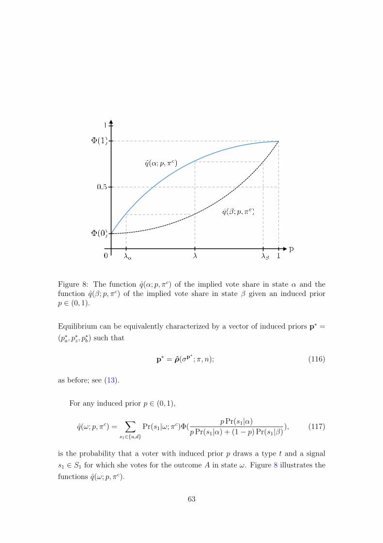
Figure 8: The function q(α; p, πc) of the implied vote share in state α and thefunction q(β; p, πc) of the implied vote share in state β given an induced priorp ∈ (0, 1).
Equilibrium can be equivalently characterized by a vector of induced priors p∗ =
(p∗a, p∗z, p∗b) such that
p∗ = ρ(σp∗ ; π, n); (116)
as before; see (13).
For any induced prior p ∈ (0, 1),
q(ω; p, πc) =∑
s1∈{u,d}
Pr(s1|ω; πc)Φ(pPr(s1|α)
pPr(s1|α) + (1− p) Pr(s1|β)), (117)
is the probability that a voter with induced prior p draws a type t and a signal
s1 ∈ S1 for which she votes for the outcome A in state ω. Figure 8 illustrates the
functions q(ω; p, πc).
63

Since Φ is continuous and strictly increasing, it follows from (17) and the
intermediate value theorem that there exists a unique belief λ such that the implied
vote shares satisfy
q(α;λ, πc)− 1
2=
1
2− q(β;λ, πc); (118)
see Figure 8. Let M = q(α;λ, πc)− 12.
The boundaries λα and λβ are such that all beliefs outside the intermediate
intervals [λα, λ] and [λ, λβ] imply margins of victory that are larger than the ones
implied by λ in any state ω ∈ {α, β}, i.e., larger than M . Formally, λα and λβ
are given by
q(α;λα, πc) = q(β;λ, πc), (119)
q(β;λβ, πc) = q(α;λ, πc). (120)
Figure 8 illustrates the boundaries λα and λβ. For a belief p > λβ,
q (β; p,π1)− 1
2> M (121)
Similarly, for p > λ,
q (α; p,π1)− 1
2> M (122)
Note that when the exogenous information πc of the voters becomes revealing
(the signal likelihood ratios of d and u go to 0 and ∞, respectively), then
λα → 0, and λβ → 1. (123)
D.2 Proof of Claim 6
The Claim 6 in the main text is stated for the information structure πr. Claim 11
below shows the analogous statement for the information structure πx,r,y, noting
(125). The same arguments imply Claim 6, and we will therefore omit its proof.
D.3 Voter Inference
We show that, when the sender provides additional information (πx,r,yn )n∈N, the
induced prior after z—and thereby the margin of victory in the states α2 and
β2—is the same across all equilibrium sequences and determined uniquely by the
exogenous information πc of the voters.
64

Claim 11 Suppose the additional information is given by (πx,r,yn )n∈N for some
(x, y) ∈ [0, 1]2 and r ∈ (0, 1), and consider the induced sequence (πn)n∈N of inde-
pendent expansions of πc. For any equilibrium sequence (σ∗n) given (πn),
limn→∞
ρz(σ∗n, πn, n) = λ. (124)
Proof. The key idea is that, for any equilibrium sequence (σ∗n)n∈N, the election is
equally close to being tied in expectation in α2 and β2 as n→∞.
limn→∞
q(σ∗n;α2, πn)− 1
2= lim
n→∞
1
2− q(σ∗n; β2, πn), (125)
by arguments similar to those from the proof of the CJT; see (22).
Since almost all voters receive z in α2 and β2, the expected vote share in
these states converges to the vote share implied by the induced prior after z; for
ω2 ∈ {α2, β2},
limn→∞
q(σ∗n;ω2, πn) = limn→∞
q(ω; ρz(σ∗n; πn, n), πc). (126)
Recall that λ is the unique induced prior such that the margins of victory are
equal given the implied vote shares; see (118). So, (125) and (126) imply the
claim, (124). It remains to show (125).
Step 1 For all n and every equilibrium σ∗n, voters with a (z, u)-signal are more
likely to vote A than voters with a (z, d)-signal when n is large enough, i.e.
Φ(ρz,u(σ∗n)) > Φ(ρz,d(σ
∗n)). (127)
This ordering follows from the likelihood ratio ordering of the signals u and d, i.e.,Pr(u|α;πc)Pr(u|β;πc)
> Pr(d|α;πc)Pr(d|β;πc)
, and the independence of πx,r,yn and πc. Using (115), we have
Pr (α|z, u, piv;σ∗n, πn, n) > Pr (α|z, d, piv;σ∗n, πn, n). Now, (127) follows from the
monotonicity of Φ.
Step 2 For all n and every equilibrium σ∗n, the vote share of A is at most 1n2
smaller in α2 than in β2,
q(α2;σ∗n)− q(β2;σ∗n) ≥ − 1
n2(128)
For signals (a, b), the ordering may be the reverse of (127). However, in α2 and
β2, the likelihood that a voter does not receive signal z is smaller than 1n2 . So, this
65

follows from (15), given (20) and (127).
Step 3 For every equilibrium sequence (σ∗n),
limn→∞
ρz(σ∗n; πn, n) /∈ {0, 1}. (129)
We have
ρz(σ∗n; πn, n)
1− ρz(σ∗n; πn, n)=
Pr(α)
Pr(β)
Pr(α2|α; πn)
Pr(β2|β; πn)
Pr(piv|α2;σ∗n, πn, n)
Pr(piv|β2;σ∗n, πn, n). (130)
Suppose that limn→∞ ρz(σ∗n; πn, n) = 0. We show that this implies
limn→∞
Pr(piv|α2;σ∗n, πn, n)
Pr(piv|β2;σ∗n, πn, n)≥ 1; (131)
a contradiction. Since almost all voters receive z in α2 and β2 and since Φ(0) < 12,
the hypothesis limn→∞ ρz(σ∗n; πn, n) = 0 implies that
limn→∞
q(α2, σ∗n) = lim
n→∞q(β2, σ
∗n) <
1
2. (132)
Recall that Φ(0) < q(ωj;σ) < Φ(1) for any strategy and any substate ωj and
note that the derivative of h(q) = q(1 − q) is bounded below by some Lipschitz
constant L > 0 on the compact interval [Φ(0),Φ(1)]. Hence, (128) implies
h(q(β2, σ∗n))(
h(q(α2, σ∗n))
h(q(β2, σ∗n))− 1) = h(q(α2, σ
∗n))− h(q(β2, σ
∗n)) ≥ − L
n2. (133)
Recall that the function h(q) = q(1 − q) is inverse U -shaped with a peak at
q = 12
and note that it follows from (17) and Φ being strictly increasing that
0 < Φ(0) < 12
and Φ(1) > 12. Since Φ(0) < q(β2;σ∗n) < Φ(1),
h(q(α2, σ∗n))
h(q(β2, σ∗n))≥ 1− L
h(q(β2 ;σn))n2≥ 1− L
Mn2(134)
forM = min (h(Φ(0)), h(Φ(1))) and all n. It follows from (7) that Pr(piv|α2;σ∗n,πn,n)Pr(piv|β2;σ∗n,πn,n)
≥(1 − L
Mn2 )n. Now, (131) follows since limn→∞(1 − LMn2 )n = 1; see the analo-
gous argument at the end of the proof of Claim 3. A similar argument excludes
limn→∞ ρz(σ∗n; πn, n) = 1 (using the analogous bound to (128)). This finishes the
proof of the step.
Step 4 In every equilibrium sequence (σ∗n)n∈N, the limit of the vote share of A is
66

larger in α2 than in β2,
limn→∞
q(α2;σ∗n) > limn→∞
q(β2;σ∗n). (135)
Since almost all voters receive z in α2 and β2, we have
limn→∞
q(α2;σ∗n) = limn→∞
q(α; ρz(σ∗n, πn, n)), (136)
limn→∞
q(β2;σ∗n) = limn→∞
q(β; ρz(σ∗n, πn, n)). (137)
From (129), the limits of the posteriors conditional being pivotal, the signal z and
the signals s ∈ {u, d} are interior, and hence, strictly ordered,
0 < limn→∞
Pr (α|z, d, piv;σ∗n, πn, n) < limn→∞
Pr (α|z, u, piv;σ∗n, πn, n) < 1. (138)
Now, (135) follows from (136), (137), and (117), given (20), (138), and since Φ is
strictly increasing.
We now finish the proof of Claim 11. It follows from (129) that voters must
not become certain conditional on being pivotal and the substate being α2 or β2,
i.e., limn→∞ Pr(α|{α2, β2}, piv;σ∗n, πn) /∈ {0, 1}. Hence, Claim 2 requires that
limn→∞
∣∣∣∣q(α2;σ∗n)− 1
2
∣∣∣∣ = limn→∞
∣∣∣∣q(β2;σ∗n)− 1
2
∣∣∣∣ . (139)
Given the ordering of the limits of the vote shares from (135), the equation (139)
implies (125). As noted, this completes the proof of Claim 11.
Consider a voter who received an additional signal s2 ∈ {a, b}. The following
result shows that the inference from the signals is dominated by the inference from
the pivotal event if the election is closer to being tied in states α2 and β2 than in
the states α1 and β1. The arguments are analogous to the ones from the proof of
Claims 4 and 8; we therefore omit the proof.
Claim 12 Suppose that the additional information is given by (πx,r,yn )n∈N for some
(x, y) ∈ [0, 1]2 and r ∈ (0, 1), and consider the corresponding sequence (πn)n∈N of
independent expansions of πc. Take any sequence of strategies (σn)n∈N such that
limn→∞
minω1∈{α1,β1}
|q(σn;ω1, πn)− 1
2| > lim
n→∞max
ω2∈{α2,β2}|q(σn;ω2, πn)− 1
2|; (140)
67
then, for any s ∈ {u, d} × {a, b},
limn→∞
Pr({α2, β2}|s, piv;σn, πn)
Pr({α1, β1}|s, piv;σn, πn)=∞. (141)
Now, take any sequence of equilibria (σ∗n)n∈N that satisfies (140). Claim 12
implies that
limn→∞
Pr(α|a, piv;σ∗n, πn, n)
Pr(β|a, piv;σ∗n, πn, n)= lim
n→∞
Pr(α2|a, piv;σ∗n, πn, n)
Pr(β2|a, piv;σ∗n, πn, n)(142)
In the following formula, we omit the dependence on σ∗n and πn. Using Bayes’
rule,35
limn→∞
Pr(α2|a, piv)
Pr(β2|a, piv)= lim
n→∞
Pr(α)
Pr(β)
Pr(α2|α)
Pr(β2|β)
Pr(a|α2)
Pr(a|β2)
Pr(piv|α2)
Pr(piv|β2)
= limn→∞
Pr(α|{α2, β2}, piv)
Pr(β|{α2, β2}, piv)
Pr(a|α2)
Pr(a|β2). (143)
Note that limn→∞ ρz(σ∗n; πn, n) = limn→∞ Pr(α|{α2, β2}, piv;σ∗n, πn, n) such that
Claim 11 implies
limn→∞
Pr(α|{α2, β2}, piv;σ∗n, πn, n) = λ. (144)
Using (142), (143), (144), and the definition of the information structure πx,r,yn , we
conclude
limn→∞
Pr(α|a, piv;σ∗n, πn)
Pr(β|a, piv;σ∗n, πn)=
x
1− xλ
1− λ. (145)
Similarly, for the additional signal b,
limn→∞
Pr(α|b, piv;σ∗n, πn, n)
Pr(β|b, piv;σ∗n, πn, n)=
y
1− yλ
1− λ. (146)
D.4 Fixed Point Argument
In this section, we prove Lemma 3, using the observations from the preceding
section. Let us consider some belief µα /∈ [λα, λ] and some belief µβ /∈ [λ, λβ] with
λ, λα, and λβ given by (118), (119) and (120).
35As before, if x = 1, that is if Pr(a|β2) = 0, using the convention 10 = ∞, the following
equality holds in the extended reals.
68

Recall from Section D.1 that equilibrium can be equivalently characterized by a
vector of beliefs p∗ = (p∗a, p∗z, p∗b) such that p∗ = ρ(σp∗ ; π, n); see (116). Now, take
any δ > 0 and let
Bδ ={p ∈ [0, 1]3 | |p− (µα, λ, µβ)| ≤ δ
}.
Take any p ∈Bδ and the corresponding strategy σp. We define a constrained
best-response function as its “truncation” to Bδ:
ρtra (σp) =
µα − δ if ρa(σ
p) < µα − δ,
µα + δ if ρa(σp) > µα + δ,
ρa(σp) else.
(147)
The components ρtrz and ρtrb are defined in the analogous way. The function ρtr(σp)
is continuous in p such that Kakutani’s theorem implies that ρtr(σp) has a fixed
point p∗ ∈ Bδ.
Any fixed point p∗ of ρtr is shown to be in the interior of Bδ when n is large
enough and δ is small enough, i.e., ρtr(σp∗) = ρ(σp∗):
Claim 13 Consider any µα /∈ [λα, λ] and any µβ /∈ [λ, λβ]. Consider the sequence
of independent expansions (πn)n∈N of πc with additional information (πx,r,yn )n∈N
where µα = xλxλ+(1−x)(1−λ)
and µβ = yλyλ+(1−y)(1−λ)
and r ∈ (0, 1).
For any δ > 0 small enough, there exists n(δ) ∈ N such that for all n ≥ n(δ),
any fixed point of ρtr is in the interior of Bδ.
Proof. Pick some p for which pz is on the boundary. We show p cannot be a fixed
point for n large enough and δ small enough. First, suppose pz = λ−δ. Then, given
σ and as n → ∞, the margin of victory in α2 is strictly smaller than the margin
of victory in β2, given the definition of λ; see (118). Hence, Claim 2 implies that
limn→∞Pr(piv|α2;σp,πx,r,yn ,n)Pr(piv|β2,σp,πx,r,yn ,n)
=∞. This implies, limn→∞ ρz(σp; πx,r,yn , n) = 1. For any
n large enough this contradicts pz = λ− δ and so p is not a fixed point of ρtr(σp).
In the same way we can exclude that pz = λ+δ for any n large enough. In general,
the same argument implies that, for n large enough, for any fixed point p∗,
ρz(σp∗) ≈ λ. (148)
Given the assumptions on µα, µβ, we can choose δ > 0 small enough such that, for
any p ∈ Bδ and the corresponding behavior σp, the expected margins of victory
69
in the states α2 and β2 are strictly smaller than the expected margins of victory
in the states α1 and β1, i.e., σp satisfies (140). Therefore, it follows from Claim
12 and (148) that (145) and (146) hold; hence, given the definition of ρ
ρa(σp∗) ≈ µα, (149)
ρb(σp∗) ≈ µβ. (150)
We conclude that any fixed point p∗ of ρtr is interior when δ is small enough and
n is large enough.
Now, we finish the proof of Lemma 3. Note that the strategy σp∗ corresponding
to any interior fixed point p∗ of ρtr is an equilibrium. Therefore, Claim 13 implies
the existence of a sequence of equilibria (σ∗n)n∈N for which (148), (149), and (150)
hold. This finishes the proof of Lemma 3.
E Media Markets: An Application
Recall the setting from Section 6.2. With probability 1− χ, the media firm sends
the message m = θ in α and m = −θ in β. With probability χ > 0, the media
firm sends a shifted message, m = θ − d in α and m = −θ − d in β for some
d 6= 0. Voters perceive the message m with noise, that is, each voter receives a
private signal s = m+ ε where ε is drawn independently from a standard normal
distribution. The information structure of the voters thus has four substates
ωi ∈ {α1, β1, α2, β2}, one for each of the four messages of the firm. Denote by
m(ωi) the message in substate ωj; we label the substates so that
m(ωi) =
θ if ωi = α1,
−θ if ωi = β1
θ − d if ωi = α2,
−θ − d if ωi = β2.
(151)
Theorem 5 Consider the setting from Section 6.2. Take any strictly increasing
Φ satisfying (17). Let d > 2θ. For every constant policy x ∈ {A,B}, there is a
sequence of equilibria (σ∗n)n∈N given d such that
limn→∞
Pr (x|σ∗n, d, n) ≥ 1− χ. (152)
70

We provide the proof for x = A. The case x = B is analogous. Recall that
the collection of critical beliefs (Pr(α|s, piv;σ))s∈R is a sufficient statistic for the
best response; see (3) and (4). For the purpose of this proof, it will turn out
more convenient to conduct the analysis in the space of vectors of expected vote
shares (q(ωj;σ))ωj∈{α1,α2,β1,β2} rather than the space of critical beliefs.36 For any
strategy σ, the vector (q(ωj;σ))ωj∈{α1,α2,β1,β2} is a sufficient statistic for the pivotal
likelihood in each state, and therefore for Pr(α|s, piv;σ), for any s ∈ R. We con-
clude that the vote share vector is also a sufficient statistic for the best response.
Given some arbitrary vector of vote shares q, let p(q) = (Pr(α|s, piv;q)s∈R be the
collection of posteriors induced by q and σq = σp(q) the unique best response in
undominated strategies given p(q); compare to (12). A strategy σ∗ is an equi-
librium if and only if σ∗ = σq for q = (q(ωj;σ∗))ωj∈{α1,α2,β1,β2}. Conversely, an
equilibrium can be described by a vector of vote shares q∗ that is a fixed point of
q→ q(ωj;σq)ωj∈{α1,α2,β1,β2}. (153)
Take δ > 0. For any q, we consider a constrained variant of the map (153),
denoted
ψ(q)→ q(ωj;σq)ωj∈{α1,α2,β1,β2} (154)
and defined sequentially across substates:
q(β2;σq) = min (1
2, q(β2;σq)),
q(α2;σq) = max (1
2, q(α2;σq)),
and
q(β1;σq) = max (q(β1;σq), q(α2;σq) + δ),
q(α1;σq) = max (q(α1;σq), q(β1;σq) + δ).
36This is because there are infinitely many critical priors, given that the distribution of thesignal s is continuous. In contrast, the vote shares vector q(ωj ;σ) is finite-dimensional. Further,the best response is not necessarily cutoff strategies (in s, for fixed t) and working with voteshares helps because it “integrates out”.
71

By definition, ψ maps to the set of vectors q = (q(ωj))ω∈{α,β},j∈{1,2} satisfying
q(β2) ≤ 1
2≤ q(α2), (155)
q(α2) + δ ≤ q(β1), (156)
q(β1) + δ ≤ q(α1) (157)
and we denote ψresn its restriction to this domain, adding the subscript n for the
dependence on the electorate size. Note that ψresn is a continuous self-map, such
that Kakutani’s fixed point theorem implies that it has a fixed point.
Proof of Theorem 5.
Step 1 For any sequence (qn)n∈N of fixed points of ψresn ,
limn→∞
|qn(α2)− 1
2| = lim
n→∞|12− qn(β2)|, (158)
and there is λ ∈ (0, 1), so that for all s ∈ R
limn→∞
Pr(α|piv, s;qn, d, n)
Pr(β|piv, s;qn, d, n)=
λ
1− λf(s|α2; d)
f(s|β2; d). (159)
Proof. It follows from the analogue of Claim 2 for the posteriors p(qn) and from
(155) - (157) that limn→∞Pr(piv|{α2,β2};qn,d,n)Pr(piv|{α1,β1};qn,d,n)
=∞. Hence,
limn→∞
Pr({α1, β1}|piv;qn, d, n) = 0. (160)
Denote by f(s|ωi; d) the density of the voter’s private signal s conditional on
the substate ωi. Given (160),
limn→∞
Pr(α|piv, s;qn, d, n)
Pr(β|piv, s;qn, d, n)= lim
n→∞
Pr(α)
Pr(β)
Pr(α2|α)
Pr(β2|β)
Pr(piv|α2;qn, d, n)
Pr(piv|β2;qn, d, n)
f(s|α2; d)
f(s|β2; d).(161)
Recall that the substate ω2 in which the firm uses the slant −d has the same
probability in each state ω ∈ {α, β}, that is, Pr(α2|α)Pr(β2|β)
= 1. Given (161),
limn→∞
Pr(α|piv, s;qn, d, n)
Pr(β|piv, s;qn, d, n)=
λ
1− λf(s|α2; d)
f(s|β2; d), (162)
for λ1−λ = limn→∞
Pr(α)Pr(β)
Pr(piv|α2;s;qn,d,n)Pr(piv|β2;s;qn,d,n)
.37
37We use the convention 10 =∞.
72
Now, we show (158). Suppose that
limn→∞
|qn(α2)− 1
2| > lim
n→∞|12− qn(β2)|. (163)
Claim 2 implies λ = 0. Together with (162), this implies
limn→∞
Pr(α|piv, s;qn, d, n) = 0 (164)
for all s ∈ R. Given (164), the vote shares of the best response satisfy limn→∞ q(β2;σqn) =
limn→∞ q(α2;σqn) = Φ(0). Since Φ(0) < 1/2 by assumption and since the con-
strained best response ψ restricts the vote shares in α2 to be weakly larger than
1/2, limn→∞ q(α2;σqn) = 12. Since qn is a fixed point, qn(α2) = q(α2;σqn), so that
limn→∞ qn(α2)− 12
= 0, which yields a contradiction to (163).
Suppose that
limn→∞
|qn(α2)− 1
2| < lim
n→∞|12− qn(β2)|. (165)
Claim 2 implies λ = 1. Together with (162), this implies
limn→∞
Pr(α|piv, s;qn, d, n) = 1 (166)
for all s ∈ R. Given (166), the vote shares of the best response satisfy limn→∞ q(β2;σqn) =
limn→∞ q(α2;σqn) = Φ(1). Since Φ(1) > 1/2 by assumption and since the con-
strained best response ψ restricts the vote shares in β2 to be weakly smaller than
1/2, limn→∞ q(β2;σqn) = 12. Since qn is a fixed point, qn(β2) = q(β2;σqn), so that
limn→∞ qn(β2)− 12
= 0, which yields a contradiction to (165).
Now, we prove (159): Note that (159) follows from (162) if we establish that
λ /∈ {0, 1}. Suppose that λ = 0. We just gave an argument showing that this
implies limn→∞ qn(α2) = 12
and limn→∞ q(β2;σqn) = Φ(0). Since Φ(0) < 1/2
and since qn is a fixed point, qn(β2) = q(β2;σqn) when n is large. Altogether,
this implies limn→∞ |qn(β2) − 12| > limn→∞ |qn(α2) − 1
2|, a contradiction to (158).
Hence, λ 6= 0. Suppose that λ = 1. We just gave an argument showing that
this implies limn→∞ qn(β2) = 12
and limn→∞ q(α2;σqn) = Φ(1). Since Φ(1) > 1/2
and since qn is a fixed point, qn(α2) = q(α2;σqn) when n is large. Altogether,
this implies limn→∞ |qn(β2) − 12| < limn→∞ |qn(α2) − 1
2|, a contradiction to (158).
Hence λ 6= 1.
73

Step 2 If m(ωj) > m(ωi): For any sequence (qn)n∈N of fixed points of ψresn ,
limn→∞ q(ωj;σqn) > limn→∞ q(ωi;σ
qn).
Proof. Take a sequence of fixed points qn. In the following, sometimes we drop
the dependence on qn, d and n from the notation. Consider the limit vote shares
of the best response,
limn→∞
q(ωi;σqn) = lim
n→∞
∫s∈R
Φ(Pr(α|piv, s;qn, d, n))f(s|ωi; d)ds,
for ωi ∈ {α1, β1, α2, β2}. We rewrite
limn→∞
q(ωi;σqn) =
∫s∈R
limn→∞
Φ(Pr(α|piv, s;qn, d, n))f(s|ωi; d)ds,
=
∫s∈R
Φ( limn→∞
Pr(α|piv, s;qn, d, n))f(s|ωi; d)ds, (167)
where we apply the dominated convergence theorem for the first equality and for
the second equality we use that Φ is continuous.Recall that the signal distributions
in the substates are normal distributions with the same variance and shifted mean.
In particular, f(s|ωi; d) = f(s + m(ωj) − m(ωi)|ωj; d) for substates ωi 6= ωj.
Therefore,
limn→∞
q(ωi) =
∫s∈R
Φ( limn→∞
Pr(α|piv, s))f(s+m(ωj)−m(ωi)|ωj; d)ds
=
∫s′∈R
Φ( limn→∞
Pr(α|piv, s′ −m(ωj) +m(ωi)))f(s′|ωj; d)ds′(168)
substituting s′ = s+m(ωj)−m(ωi). Now,
limn→∞
q(ωj) =
∫s′∈R
Φ( limn→∞
Pr(α|piv, s′))f(s|ωj)ds′
>
∫s′∈R
Φ( limn→∞
Pr(α|piv, s′ −m(ωj) +m(ωi)))f(s′|ωj)ds′ (169)
where the equality simply restates (167) and we claim that the inequality (169)
holds if m(ωj) > m(ωi). To see why (169) holds, recall (159), which says that there
is λ ∈ (0, 1) so that limn→∞Pr(α|piv,s′)Pr(β|piv,s′)
= λ1−λ
f(s|α2;d)f(s|β2;d)
for all s′ ∈ R. The likelihood
ratio f(s|α2;d)f(s|β2;d)
is strictly increasing in s since the mean of the normal in α2 is higher
than the mean of the normal in β2. Together, we obtain limn→∞ Pr(α|piv, s′) >
limn→∞ Pr(α|piv, s′−m(ωj)+m(ωi)) for all s′ ∈ R if m(ωj) > m(ωi). This implies
74

the inequality (169) since we assumed that Φ is strictly increasing. Finally, (168)
and (169) together show limn→∞ q(ωj;σqn) > limn→∞ q(ωi;σ
qn).
Step 3 For any sequence (qn)n∈N of fixed points of ψresn ,
limn→∞
q(α2;σqn) >1
2> lim
n→∞q(β2;σqn). (170)
Proof. Suppose that limn→∞ q(α2;σqn) ≤ 1/2. Then, limn→∞ q(α2;σqn) = 1/2
by the definition of q. Given (151), m(α2) > m(β2), so that Step 2 implies
limn→∞ q(β2;σqn) < 1/2. But this means that (158) does not hold, , which cannot
be. Hence, limn→∞ q(α2;σqn) > 1/2. Similarly, suppose that limn→∞ q(β2;σqn) ≥1/2. Then, limn→∞ q(β2;σqn) = 1/2. Since m(α2) > m(β2), Step 2 implies
limn→∞ q(α2;σqn) > 1/2. But this means that (158) does not hold, which cannot
be. Hence, limn→∞ q(β2;σqn) < 1/2.
Step 4 For any sequence (qn)n∈N of fixed points of ψresn , there is n ∈ N so that
for n ≥ n, the fixed point qn is interior.
Proof. The assumption d > 2θ implies θ − d < −θ so that the messages in the
substates are ordered as
m(β2) < m(α2) < m(β1) < m(α1), (171)
given (151). Applying Step 2,
limn→∞
q(β2;σqn) < limn→∞
q(α2;σqn) < q(β1;σqn) < q(α1;σqn). (172)
So, the limit vote shares differ pair-wise by at least some δ′ > 0. We claim that
δ′ > 0 does not depend on the bound δ > 0 in the definition of ψresn , so that we can
choose δ < δ′/2. To see why, note that the limit vote share in ωi only depends on
λ, on the message m(ωi), and on the preference distribution Φ, given (162) and
(167). Further, λ is fixed by the equal-margin condition (158). We conclude that
differences in the limit vote shares do not depend on δ.
The inequalities (172) and (170) together with the lower bound δ′ > 0 and δ <δ′
2imply that the vector of vote shares q(ωi;σ
qn) satisfies (155) - (157) when n is
large enough. Since qn is a fixed point of ψresn , this implies that q(ωi;σ
qn) = qn(ωi)
for all ωi ∈ {α1, α2, β1, β2}, meaning that the fixed point of ψresn is interior.
We finish the proof of Theorem 5. Take any sequence of fixed points (qn)n∈N of
ψresn . Step 4 implies that the fixed point qn corresponds to an equilibrium σqn when
75

n is sufficiently large. This shows the existence of an equilibrium sequence, and
this sequence satisfies (170) and (172). It follows from the law of large numbers
that policy A is elected with probability converging to 1 as n→∞ in each of the
sub-states α1, α2, and β1, which occur with a joint probability larger than 1− ψ.
This proves the claim (173) of Theorem 5.�
E.1 Multiple Media Firms
Theorem 6 Consider the setting from Section 6.3. Take any strictly increasing
Φ satisfying (17). Let d > 2θ. For every constant policy x ∈ {A,B}, there is a
sequence of equilibria (σ∗n)n∈N given d such that
limn→∞
Pr (x|σ∗n, d, n) ≥ 1− χ. (173)
The proof of Theorem 6 is almost verbatim to the proof of Theorem 5, and there-
fore omitted.
The key observation is that in the setting with multiple media firms, there are
still the four relevant substates from the setting with a monopolistic media firm
and we can work with the vector of vote shares in the same way as in the proof of
Theorem 5 for the monopolistic case. Additionally, we note that for each substate
ωi and pair s = (s1, s2),
f(s|ωi; d) = f(s1|ωi)f(s2|ωi; d)
since the signals s1 and s2 are independent conditional on the state; further, the
relevant substitution in the analogue of (168) is s′2 = s2 +m2(ωj)−m2(ωi). That
is, in the analogous step, we leverage that f(s2|ωi) = f(s2 +m2(ωj)−m2(ωi)|ωj),which holds by the definition of the distribution of the private signal s2 in the
substates.
F Persuasion of Behavioral Types: Numerical
Example
Consider a belief p = (pa, pz) and the corresponding strategy σp. Consider the
information structure πn = πrn from Figure 4. In the following, we omit the
76

dependence on σp and on πn most of the time. We have
Pr(α|z; πrn)
Pr(β|z; πrn)=
Pr(α)
Pr(β)
Pr(α2|α)
Pr(β2|β)
Pr(z|α2)
Pr(z|β2)(174)
=1
22(1− 1
n2), (175)
and
Pr(α|a; πrn)
Pr(β|a; πrn)=
Pr(α)
Pr(β)
∑i=1,2 Pr(αi|α) Pr(a|αi)∑i=1,2 Pr(βi|α) Pr(a|βi)
(176)
=1
2
(1− 3n) + 3
n3 )
1− 1n
. (177)
Let q(ωi;σp, κ, n) the expected vote share in a substate ωi when there is a frac-
tion κ = 0.4 of sincere voters, who vote according to σp′ for p′ = (Pr(α|a),Pr(α|z)),
and a fraction 1 − κ = 0.6 of pivotal voters who vote according to σp. Simi-
larly, ρ(σp) = (Pr(α|a, piv;σp, κ),Pr(α|z, piv;σp, κ)) is the vector of induced pri-
ors given by the vote shares q(ωi;σp, κ, n) through (6) and (7).
Fixed Point Argument. Take any p = (pa, pz) with
pa ≥ 0.99, (178)
pz ∈ [0.475, 0.525]. (179)
For n ≥ 84 and κ = 0.4, we have the following bounds for the expected vote
share for policy A:
q(ω1;σp, κ, n) ≥ κ0.328 + (1− κ)0.99 (180)
≥ 0.725 for ω1 ∈ {α1, β1}, (181)
q(α2;σp, κ, n) > 0.475 (182)
q(β2;σp, κ, n) ≤ 0.525. (183)
Step 1 For any n ≥ 84 and any ω1 ∈ {α1, β1}, ω′2 ∈ {α2, β2},
Pr(piv|ω′2)
Pr(piv|ω1)≥ (1.25)n (184)
77

The step follows from,
Pr(piv|ω′2)
Pr(piv|ω1)
≥ [1 + minω1,ω′2
(q(ω1;σp)− 12)2 − (q(ω′2;σp)− 1
2)2
14− (q(ω1;σp)− 1
2)2
]n
≥ (1 + (( 9
40)2 − ( 1
40)2
14− ( 9
40)2
))
≥ (1 +80
319)n
≥ (1.25)n. (185)
where we used Lemma 2 and that 0.725 = 2940
, 0.475 = 1940
, and 0.525 = 2140
for the
inequality on the second line, and dropped κ and n from the notation for the vote
shares.
Step 2 For n ≥ 84: ρa(σp) ≥ 0.99, and ρz(σ
p) ∈ [0.475, 0.525].
First,
ρa(σp)
1− ρa(σp)≥ p0
1− p0
Pr(α2|α) Pr(b|α2) Pr(piv|α2)
Pr(β1|β) Pr(b|β1) Pr(piv|β1)
≥ 1
3
3n
1n2
(1− 1n)(1.25)n
≥ 100 for n ≥ 84,
where we used (83) for the inequality on the second line. Hence, for n ≥ 84,
ρ(σp)a ≥100
101> 0.99. (186)
Second,
Pr(piv|α2)
Pr(piv|β2)≤ [1 +
|(q(β2;σp)− 12)2 − (q(α2;σp)− 1
2)2|
14− (q(β2;σp)− 1
2)2
]n
≤ (1 +1n4 + 1
n2
14− 81
402
)n
≤ 1.08. for n ≥ 84.
where we used Lemma 2 for the inequality on the first line. For the inequality
on the second line, we used that z is sent with probability 1 − 1n2 in both α2
78

and β2 such that the difference in the squared margins of victory cannot exceed
(x+ 1n2 )2 − x2 ≤ 2x
n2 + 1n4 where x is the minimum margin of victory in the states
α2, β2. Finally, the inequality follows since the margin of victory in both α2 and
β2 is bounded by 0.2. So,
ρz(σp)z
1− ρz(σp)=
Pr(α)
Pr(β)
Pr(α2|α)
Pr(β2|β)
Pr(z|α2)
Pr(z|β2)
Pr(piv|α2)
Pr(piv|β2)
= (1− 1
n2)Pr(piv|α2)
Pr(piv|β2)
≤ 1.08 for n ≥ 84.
Consequently, for all n ≥ 84,
ρ(σp)z ≤1.08
2.08< 0.52 (187)
Third,
Pr(piv|α2)
Pr(piv|β2)≥ (1−
|(q(β2;σp)− 12)2 − (q(α2;σp)− 1
2)2|
14− (q(β2;σp)− 1
2)2
≥ (1−1n4 + 1
n2
14− 81
402
)n
≥ 0.934 for n ≥ 84. (188)
So, for all n ≥ 84,
ρ(σp)z1− ρ(σp)z
= (1− 1
n2)Pr(piv|α2;σp)
Pr(piv|β2;σp)≥ 0.93.
This gives for all n ≥ 84,
ρ(σp)z ≥0.93
1 + 0.93≥ 0.48. (189)
The claim follows from (186), (187)), and (189).
Step 3 For n ≥ 84, there is an equilibrium σ∗n which satisfies (180) - (183).
It follows from Step 2 that, for any n ≥ 84, the continuous map that sends p to
ρ(σp) is a self-map on the set of beliefs that satisfy (178) - (179). It follows from
the Kakutani fixed point theorem that there exists fixed points p∗n that satisfy
79

(178) - (179). The corresponding strategies σp∗n are equilibria (compare to (13))
and they satisfy (180) - (183).
Step 4 Given the equilibrium σ∗n for n ≥ 84, the probability that A is elected is
larger than 99.9%.
Evaluation of the binomial distribution shows that Pr(B(2n + 1, x)) > n) ≥0.999999 if n ≥ 84 and x ≥ 0.725. Hence, given σ∗n, A is elected with proba-
bility larger than 99.9% in the states α1 and β1. Finally, the claim follows since
these states occur with probability (1− r1−r
1n) = (1− 2
n) and (1− 1
n) respectively.
The fourth step finishes the calculations for the example.
80