Partial Least Squares Structural Equation Modeling...

Marketing Bulletin, 2013, 24, Technical Note 1

Partial Least Squares Structural Equation Modeling (PLS-SEM) Techniques

Using SmartPLS

Ken Kwong-Kay Wong SmartPLS is one of the prominent software applications for Partial Least Squares Structural Equation Modeling (PLS-SEM). It was developed by Ringle, Wende & Will (2005). The software has gained popularity since its launch in 2005 not only because it is freely available to academics and researchers, but also because it has a friendly user interface and advanced reporting features. Although an extensive number of journal articles have been published on the topic of PLS modeling, the amount of instructional materials available for this software is limited. This paper is written to address this knowledge gap and help beginners to understand how PLS-SEM can be used in marketing research. Keywords: Partial Least Squares, Structural Equation Modeling, PLS-SEM, SmartPLS, Marketing,

Retail Management Introduction Structural Equation Modeling (SEM) is a second-generation multivariate data analysis method that is often used in marketing research because it can test theoretically supported linear and additive causal models (Chin, 1996; Haenlein & Kaplan, 2004; Statsoft, 2013). With SEM, marketers can visually examine the relationships that exist among variables of interest in order to prioritize resources to better serve their customers. The fact that unobservable, hard-to-measure latent variables1 can be used in SEM makes it ideal for tackling business research problems. There are two submodels in a structural equation model; the inner model2 specifies the relationships between the independent and dependent latent variables, whereas the outer model3 specifies the relationships between the latent variables and their observed indicators4 (see Figure 1). In SEM, a variable is either exogenous or endogenous. An exogenous variable has path arrows pointing outwards and none leading to it. Meanwhile, an endogenous variable5 has at least one path leading to it and represents the effects of other variable(s).

1 Latent variables are underlying variables that cannot be observed directly, they are also known as constructs or factors. 2 The inner model is also known as a structural model. 3 The outer model is also known as a measurement model. 4 Observed indicators can be measured directly, they act as indicators for an underlying latent variable. 5 Depending on the SEM design, a variable can technically act as an independent variable or a dependent variable for different parts of the model; as long as a variable has path leading to it (i.e., arrows pointing to it from another variable), it is categorized as endogenous.

of 32 http://marketing-bulletin.massey.ac.nz


Figure 1: Inner vs. Outer Model in a SEM Diagram

Different Approaches to SEM There are several distinct approaches to SEM: The first approach is the widely applied Covariance-based SEM (CB-SEM)6, using software packages such as AMOS, EQS, LISREL and MPlus. The second approach is Partial Least Squares (PLS), which focuses on the analysis of variance and can be carried out using PLS-Graph, VisualPLS, SmartPLS, and WarpPLS. It can also be employed using the PLS module in the “r” statistical software package. The third approach is a component-based SEM known as Generalized Structured Component Analysis (GSCA); it is implemented through VisualGSCA or a web-based application called GeSCA. Another way to perform SEM is called Nonlinear Universal Structural Relational Modeling (NEUSREL), using NEUSREL’s Causal Analytics software. Faced with various approaches to path modeling, one has to consider their advantages and disadvantages to choose an approach to suit.

6 Covariance-based SEM (CB-SEM) is also known as Covariance Structure Analysis (CSA)



(i) CB-SEM: CB-SEM has been widely applied in the field of social science during the past several decades, and is still the preferred data analysis method today for confirming or rejecting theories through testing of hypothesis, particularly when the sample size is large, the data is normally distributed, and most importantly, the model is correctly specified. That is, the appropriate variables are chosen and linked together in the process of converting a theory into a structural equation model (Hair, Ringle, & Smarted, 2011; Hwang et al., 2010; Reinartz, Haenlein, & Henseler, 2009). However, many industry practitioners and researchers note that, in reality, it is often difficult to find a data set that meets these requirements. Furthermore, the research objective may be exploratory, in which we know little about the relationships that exist among the variables. In this case, marketers can consider PLS. (ii) PLS-SEM: PLS is a soft modeling approach to SEM with no assumptions about data distribution (Vinzi et al., 2010). Thus, PLS-SEM becomes a good alternative to CB-SEM when the following situations are encountered (Bacon, 1999; Hwang et al., 2010; Wong, 2010):

1. Sample size is small. 2. Applications have little available theory. 3. Predictive accuracy is paramount. 4. Correct model specification cannot be ensured.

It is important to note that PLS-SEM is not appropriate for all kinds of statistical analysis. Marketers also need to be aware of some weaknesses of PLS-SEM, including:

1. High-valued structural path coefficients are needed if the sample size is small. 2. Problem of multicollinearity if not handled well. 3. Since arrows are always single headed, it cannot model undirected correlation. 4. A potential lack of complete consistency in scores on latent variables may result in

biased component estimation, loadings and path coefficients. 5. It may create large mean square errors in the estimation of path coefficient loading.

In spite of these limitations, PLS is useful for structural equation modeling in applied research projects especially when there are limited participants and that the data distribution is skewed, e.g., surveying female senior executive or multinational CEOs (Wong, 2011). PLS-SEM has been deployed in many fields, such as behavioral sciences (e.g., Bass et al, 2003), marketing (e.g., Henseler et al., 2009), organization (e.g., Sosik et al., 2009), management information system (e.g., Chin et al., 2003), and business strategy (e.g., Hulland, 1999).



(iii) GSCA & Other Approach: If overall measures of model fit are required, or in projects where non-linear latent variables exist and have to be accommodated, GSCA may be a better choice than PLS for running structural equation modeling (Hwang et al., 2010). And for data sets that demonstrate significant nonlinearities and moderation effects among variables, the NEUSREL approach may be considered (Frank and Hennig-Thurau, 2008). However, since GSCA and NEUSREL are relatively new approaches in SEM, the amount of literature for review is limited. Marketers may find it difficult to locate sufficient examples to understand how these emerging SEM approaches can be used in different business research scenarios. Evolution of PLS-SEM Software Although developed in the mid-1960s (Wold, 1973, 1985), there has been a lack of advanced yet easy-to-use PLS path modeling software (not to be confused with PLS regression as it is different from PLS-SEM) until mid 2000s. The first generation of PLS-SEM software that was commonly used in the 1980s included LVPLS 1.8 but it was a DOS-based program. The subsequent arrival of PLS-Graph and VisualPLS added a graphical interface but they have received no significant updates since their initial releases. PLS-SEM can be performed in “r” but it requires certain level of programming knowledge. Therefore, it may not be suitable for those marketers who do not have strong computer science background. The remaining PLS-SEM software packages, still in active development, include WarpPLS (a commercial software7) and SmartPLS (a free software). This paper focuses on SmartPLS because it is freely available to the research community across the globe. Furthermore, this software has maintained an active online discussion forum8, providing a good platform for knowledge exchange among its users. Determination of Sample Size in PLS-SEM No matter which PLS-SEM software is being used, some general guidelines should be followed when performing PLS path modeling. This is particularly important, as PLS is still an emerging multivariate data analysis method, making it easy for researchers, academics, or even journal editors to let inaccurate applications of PLS-SEM go unnoticed. Determining the appropriate sample size is often the first headache faced by researchers. In general, one has to consider the background of the model, the distributional characteristics of the data, the psychometric properties of variables, and the magnitude of their relationships when determining sample size. Hair et al. (2013) suggest that sample size can be driven by the following factors in a structural equation model design:

7 WrapPLS has a 90-day fully functional free trial version that can be downloaded from the developer’s web site. 8 Online forum is located at the developer’s web site (http://www.smartpls.de).



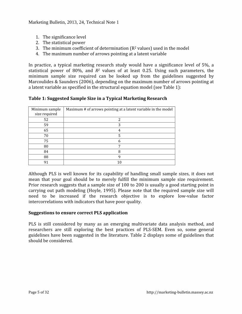
1. The significance level 2. The statistical power 3. The minimum coefficient of determination (R2 values) used in the model 4. The maximum number of arrows pointing at a latent variable

In practice, a typical marketing research study would have a significance level of 5%, a statistical power of 80%, and R2 values of at least 0.25. Using such parameters, the minimum sample size required can be looked up from the guidelines suggested by Marcoulides & Saunders (2006), depending on the maximum number of arrows pointing at a latent variable as specified in the structural equation model (see Table 1): Table 1: Suggested Sample Size in a Typical Marketing Research

Minimum sample

size required Maximum # of arrows pointing at a latent variable in the model

52 2 59 3 65 4 70 5 75 6 80 7 84 8 88 9 91 10

Although PLS is well known for its capability of handling small sample sizes, it does not mean that your goal should be to merely fulfill the minimum sample size requirement. Prior research suggests that a sample size of 100 to 200 is usually a good starting point in carrying out path modeling (Hoyle, 1995). Please note that the required sample size will need to be increased if the research objective is to explore low-value factor intercorrelations with indicators that have poor quality. Suggestions to ensure correct PLS application PLS is still considered by many as an emerging multivariate data analysis method, and researchers are still exploring the best practices of PLS-SEM. Even so, some general guidelines have been suggested in the literature. Table 2 displays some of guidelines that should be considered.



Table 2: Some Guidelines on PLS Applications

Topics: Suggestions: References: Measurement scale Avoid using a categorical scale

in endogenous constructs Hair et al., 2010

Value for outer weight Use a uniform value of 1 as starting weight for the approximation of the latent variable score

Henseler, 2010

Maximum number of iterations

300 Ringle et al., 2005

Bootstrapping Number of bootstrap “samples” should be 5000 and number of bootstrap “cases” should be the same as the number of valid observations

Hair et al., 2011

Inner model evaluation Do not use goodness-of-fit (GoF) Index9

Henseler and Sarstedt, 2013

Outer model evaluation (reflective)

Report indicator loadings. Do not use Cronbach’s alpha for internal consistency reliability.

Bagozzi and Yi, 1988

Outer model evaluation (formative)

Report indicator weights. To test the outer model’s significance, report t-values, p-values and standard errors

-

SmartPLS applied: An example The following customer satisfaction example will be used to demonstrate how to use the SmartPLS software application. Customer satisfaction is an example of a latent variable that is multidimensional and difficult to observe directly. However, one can measure it indirectly with a set of measurable indicators10 that serve as proxy. In order to understand customer satisfaction, a survey can be conducted to ask restaurant patrons about their dining experience. In this fictitious survey example, restaurant patrons are asked to rate their experience on a scale representing four latent variables, namely Customer Expectation (EXPECT), Perceived Quality (QUAL), Customer Satisfaction (SAT), and Customer Loyalty (LOYAL), using a 7-point Likert scales11 [(1) strongly disagree, (2) disagree, (3) somewhat disagree, (4) neither agree nor disagree, (5) somewhat agree, (6) agree, and (7) strongly agree]. The conceptual framework is visually shown in Figure 2, and the survey questions asked are presented in Table 3. Other than Customer Satisfaction (SAT) that is measured by one question, all other variables (QUAL, EXPECT, & LOYAL) are each measured by three questions. This design is in line with similar researches conducted for the retail industry (Hair et al., 2013).

9 The Goodness-of-fit (GoF) index is an index measuring the predictive performance of the measurement model. Specifically, it can be understood as the geometric mean of the average communality and the average R2 of the endogenous latent variables. See Esposito Vinzi et al. (2008, p. 444) and Henseler & Sarstedt (2013, p570) 10 Indicators are also known as items or manifest variables. 11 An alternative approach is to use a 10-point Likert scale.



Figure 2: Conceptual Framework – Restaurant Example

Table 3: Questions for Indicator Variables

Customer Expectation (EXPECT) expect_1 [this restaurant] has the best menu selection. expect_2 [this restaurant] has the great atmospheric elements. expect_3 [this restaurant] has good looking servers.

Perceived Quality (QUAL) qual_1 The food in [this restaurant] is amazing with great taste. qual_2 Servers in [this restaurant] are professional, responsive, and friendly. qual_3 [this restaurant] provides accurate bills to customers.

Customer Satisfaction (SAT) cxsat If you consider your overall experiences with [this restaurant], how satisfied are

you with [this restaurant]? Customer Loyalty (LOYAL)

loyal_1 I would recommend [this restaurant] to my friends and relatives. loyal_2 I would definitely dine at [this restaurant] again in the near future. loyal_3 If I had to choose again, I would choose [this restaurant] as the venue for this

dining experience.



Installing the SmartPLS software application SmartPLS can be downloaded for free from the software developer’s official website at www.smartpls.de. A free account registration is required prior to downloading the software (see Figure 3). Since SmartPLS is primarily designed for the academic community, the account set up request is manually reviewed by the software developer team in Germany. It may take up to a few business days to set up an account with SmartPLS as the process is not automatic. Figure 3: SmartPLS Account Registration

The SmartPLS software application can be found in the “Downloads” section located in the upper right hand corner of the discussion forum page (see Figure 4). Microsoft Windows user should download the “win32 (win32/x86)” version for installation. Although SmartPLS is written in Java, Intel-based Apple Mac users should utilize visualization software12 or Apple’s own Bootcamp function to run SmartPLS under the Windows OS environment13. This is because the “Macosx (carbon/ppc)” version is not compatible with the latest MacOS (e.g., 10.7, 10.8 and 10.9). The software requires a personal SmartPLS activation key to run and it can be generated by pressing the “My Key” link on the same web page. Please note that such activation key has to be renewed every three months for continuous usage of the software.

12 Examples include VMware Fusion, Parallels Desktop, and Oracle’s VirtualBox. 13 Examples include Windows XP, VISTA, 7 and 8.


http://www.smartpls.de/


Figure 4: SmartPLS Discussion Forum

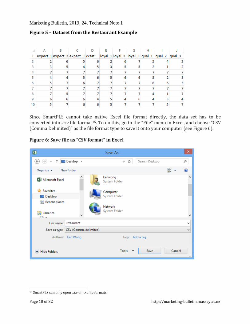
Data Preparation for SmartPLS In this restaurant example, the survey data were manually typed into Microsoft Excel and saved as .xlsx format (see Figure 5). This data set has a sample size of 400 without any missing values, invalid observations or outliers. To ensure SmartPLS can import the Excel data properly, the names of those indicators (e.g., expect_1, expect 2, expect_3) should be placed in the first row of an Excel spreadsheet, and that no “string” value (e.g., words or single dot14) is used in other cells.

14 A single dot “.” is usually generated by IBM SPSS Statistics to represent a missing value.



Figure 5 – Dataset from the Restaurant Example

Since SmartPLS cannot take native Excel file format directly, the data set has to be converted into .csv file format15. To do this, go to the “File” menu in Excel, and choose “CSV (Comma Delimited)” as the file format type to save it onto your computer (see Figure 6). Figure 6: Save file as “CSV format” in Excel

15 SmartPLS can only open .csv or .txt file formats



Project Creation in SmartPLS Now, launch the SmartPLS program and go to the “File” menu to create a new project. We will name this project as “restaurant” and then import the indicator data. Since there is no missing value16 in this restaurant data set, we can press the “Finish” button to create the PLS file. Once the data set is loaded properly into SmartPLS, click the little “+” sign next to restaurant to open up the data in the “Projects” tab. (see Figure 7). Figure 7: Project Selection

Under the “restaurant” project directory, a “restaurant.splsm” PLS file and a corresponding “restaurant.csv” data file are displayed17. Click on the first one to view the manifest variables under the “Indicators” tab (see Figure 8).

16 For other data sets that include missing values, a replacement value of “-9999” is suggested. However, please note that you can only specify a single value for all missing data in SmartPLS. 17 For each project, you can have more than one path model (i.e., the .splsm file) and dataset (i.e., .csv file).



Figure 8: List of Indicators

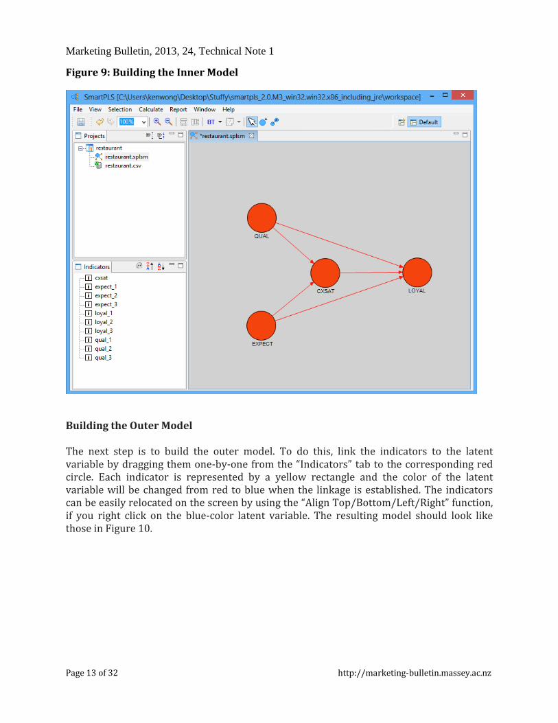
Building the Inner Model Based on the conceptual framework that has been designed earlier in this paper (see Figure 2), an inner model can be built easily in SmartPLS by first clicking on the modeling window on the right hand side, and then selecting the 2nd last blue-color circle icon titled “Switch to Insertion Mode”. Click in the window to create those red-color circles that represent your latent variables. Once the circles are placed, right click on each latent variable to change the default name into the appropriate variable name in your model. Press the last icon titled “Switch to Connection Mode” to draw the arrows to connect the variables together (see Figure 9).



Figure 9: Building the Inner Model

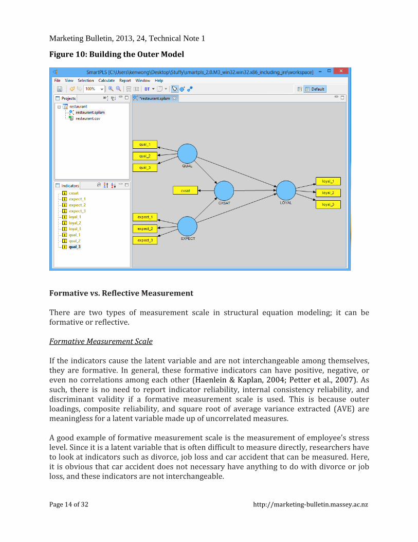
Building the Outer Model The next step is to build the outer model. To do this, link the indicators to the latent variable by dragging them one-by-one from the “Indicators” tab to the corresponding red circle. Each indicator is represented by a yellow rectangle and the color of the latent variable will be changed from red to blue when the linkage is established. The indicators can be easily relocated on the screen by using the “Align Top/Bottom/Left/Right” function, if you right click on the blue-color latent variable. The resulting model should look like those in Figure 10.



Figure 10: Building the Outer Model

Formative vs. Reflective Measurement There are two types of measurement scale in structural equation modeling; it can be formative or reflective. Formative Measurement Scale If the indicators cause the latent variable and are not interchangeable among themselves, they are formative. In general, these formative indicators can have positive, negative, or even no correlations among each other (Haenlein & Kaplan, 2004; Petter et al., 2007). As such, there is no need to report indicator reliability, internal consistency reliability, and discriminant validity if a formative measurement scale is used. This is because outer loadings, composite reliability, and square root of average variance extracted (AVE) are meaningless for a latent variable made up of uncorrelated measures. A good example of formative measurement scale is the measurement of employee’s stress level. Since it is a latent variable that is often difficult to measure directly, researchers have to look at indicators such as divorce, job loss and car accident that can be measured. Here, it is obvious that car accident does not necessary have anything to do with divorce or job loss, and these indicators are not interchangeable.



When formative indicators exist in the model, the direction of the arrows has to be reversed. That is, the arrow should be pointing from the yellow-color formative indicators to the blue-color latent variable in SmartPLS. This can be done easily by right clicking on the latent variable and selecting “Invert measurement model” to change the arrow direction. Reflective Measurement Scale If the indicators are highly correlated and interchangeable, they are reflective and their reliability and validity should be thoroughly examined (Haenlein & Kaplan, 2004; Hair et al., 2013; Petter et al., 2007). For example, the latent variable Perceived Quality (QUAL) in our restaurant data set is made up of three observed indicators: food taste, server professionalism, and bill accuracy. Their outer loadings, composite reliability, AVE and its square root should be examined and reported. In a reflective measurement scale, the causality direction is going from the blue-color latent variable to the yellow-color indicators. It is important to note that by default, SmartPLS assumes the indicators are reflective when the model is built, with arrows pointing away from the blue-color latent variable. One of the common mistakes that researchers made when using SmartPLS is that they forget to change the direction of the arrows when the indicators are “formative” instead of “reflective”. Since all of the indicators in this restaurant example are reflective, there is no need to change the arrow direction. We will continue to explore this reflective example and once the PLS-SEM analysis is done, discussion of a formative measurement model will follow. Running the Path-Modeling Estimation Once the indicators and latent variables are linked together successfully in SmartPLS (i.e., no more red-color circles and arrows), the path modeling procedure can be carried out by going to the “Calculate” menu and selecting “PLS Algorithm”. If the menu is dimmed, just click on the main modeling window to activate it. A pop-up window will be displayed to show the default settings. Since there is no missing value18 for our data set, we proceed directly to the bottom half of the pop-up window to configure the “PLS Algorithm – Settings” with the following parameters (see Figure 11):

1. Weighting Scheme: Path Weighting Scheme 2. Data Metric: Mean 0, Variance 1 3. Maximum Iterations: 300 4. Abort Criterion: 1.0E-5 5. Initial Weights: 1.0

18 If there is a missing value in your dataset, choose “Mean Value Replacement” rather than “Case Wise Deletion”, as it is the recommended option for PLS-SEM.



Figure 11: Configuring the PLS Algorithm

To run the path modeling, press the “Finish” button. There should be no error messages19 popping up on the screen, and the result can now be assessed and reported. Assessing the PLS-SEM Output For an initial assessment of PLS-SEM model, some basic elements should be covered in your research report. If a reflective measurement model is used, as in our restaurant example, the following topics have to be discussed:

• Explanation of target endogenous variable variance • Inner model path coefficient sizes and significance • Outer model loadings and significance • Indicator reliability • Internal consistency reliability • Convergent validity20 • Discriminant validity • Checking Structural Path Significance in Bootstrapping

19 If your data set has an indicator that includes too many identical values, the variance will become zero and lead to a “singular data matrix” error. To fix it, simply remove that indicator from your model. 20 Note that convergent validity and discriminant validity are measures of construct validity. They do not negate the need for considered selection of measures for proper content and face validity.



On the other hand, if the model has a formative measurement, the following should be reported instead:

• Explanation of target endogenous variable variance • Inner model path coefficient sizes and significance • Outer model weight and significance • Convergent validity • Collinearity among indicators

SmartPLS presents path modeling estimations not only in the Modeling Window but also in a text-based report21 which is accessible via the “Report” menu. In the PLS-SEM diagram, there are two types of numbers:

1. Numbers in the circle: These show how much the variance of the latent variable is being explained by the other latent variables.

2. Numbers on the arrow: These are called the path coefficients. They explain how strong the effect of one variable is on another variable. The weight of different path coefficients enables us to rank their relative statistical importance.22

Figure 12: PLS-SEM Results

21 Default Report is the preferred one. You can also choose HTML Report or LaTex Report depending on your needs. 22 In general, for data set that has up to 1000 observations or samples, the “standardized” path coefficient should be larger than 0.20 in order to demonstrate its significance. Also note that the relative statistical importance of a variable is not the same as its strategic or operational importance.



The PLS path modeling estimation for our restaurant example is shown in Figure 12. By looking at the diagram, we can make the following preliminary observations: (i) Explanation of target endogenous variable variance The coefficient of determination, R2, is 0.572 for the LOYAL endogenous latent

variable. This means that the three latent variables (QUAL, EXPECT, and CXSAT) moderately23 explain 57.2% of the variance in LOYAL.

QUAL and EXPECT together explain 30.8% of the variance of CXSAT.24 (ii) Inner model path coefficient sizes and significance

The inner model suggests that CXSAT has the strongest effect on LOYAL (0.504),

followed by QUAL (0.352) and EXPECT (0.003). The hypothesized path relationship between QUAL and LOYAL is statistically

significant. The hypothesized path relationship between CXSAT and LOYAL is statistically

significant. However, the hypothesized path relationship between EXPECT and LOYAL is not

statistically significant25. This is because its standardized path coefficient (0.003) is lower than 0.1. Thus we can conclude that: CXSAT and QUAL are both moderately strong predictors of LOYAL, but EXPECT does not predict LOYAL directly.

(iii) Outer model loadings To view the correlations between the latent variable and the indicators in its outer model, go to “Report” in the menu and choose “Default Report”. Since we have a reflective model in this restaurant example, we look at the numbers as shown in the “Outer Loadings”26 window (PLS Calculation Results Outer Loadings). We can press the “Toggle Zero Values” icon to remove the extra zeros in the table for easier viewing of the path coefficients (see Figure 13).

23 In marketing research, R2 of 0.75 is substantial, 0.50 is moderate, and 0.25 is weak. 24 CXSAT acts as both independent and dependent variable in this example and is placed in the middle of the model. It is considered to be an endogenous variable as it has arrows pointing from other latent variables (QUAL and EXPECT) to it. As a rule of thumb, exogenous variable only has arrows pointing away from it. 25 In SmartPLS, the bootstrap procedure can be used to test the significance of a structural path using T-Statistic. This topic is discussed later in the paper. 26 If a “formative” measurement model is used, view “Outer Weights” instead.



Figure 13: Path Coefficient Estimation in the Outer Model

In SmartPLS, the software will stop the estimation when (i) the stop criterion of the algorithm was reached, or (ii) the maximum number of iterations has reached, whichever comes first. Since we intend to obtain a stable estimation, we want the algorithm to converge before reaching the maximum number of iterations. To see if that is the case, go to “Stop Criterion Changes” (see Figure 14) to determine how many iterations have been carried out. In this restaurant example, the algorithm converged only after 4 iterations (instead of reaching 300), so our estimation is good27.

27 If the PLS-SEM algorithm cannot converge your data in less than 300 iterations, it means that your data is abnormal (e.g., sample size too small, existence of outliers, too many identical values in indicator) and requires further investigation.



Figure 14: Stop Criterion Changes Table

(iv) Indicator reliability28 Just like all other marketing research, it is essential to establish the reliability and validity of the latent variables to complete the examination of the structural model. The following table shows the various reliability and validity items that we must check and report when conducting a PLS-SEM (see Table 4).

28 Do not report indicator reliability if a “formative” measurement is used.



Table 4: Checking Reliability and Validity

What to check? What to look for in SmartPLS?

Where is it in the report?

Is it OK?

Reliability Indicator Reliability “Outer loadings”

numbers PLSCalculation ResultsOuter Loadings

Square each of the outer loadings to find the indicator reliability value. 0.70 or higher is preferred. If it is an exploratory research, 0.4 or higher is acceptable. (Hulland, 1999)

Internal Consistency Reliability

“Reliability” numbers PLSQuality CriteriaOverview

Composite reliability should be 0.7 or higher. If it is an exploratory research, 0.6 or higher is acceptable. (Bagozzi and Yi, 1988)

Validity Convergent validity “AVE” numbers

PLSQuality CriteriaOverview

It should be 0.5 or higher (Bagozzi and Yi, 1988)

Discriminant validity “AVE” numbers and Latent Variable Correlations

PLSQuality CriteriaOverview (for the AVE number as shown above) PLSQuality CriteriaLatent Variable Correlations

Fornell and Larcker (1981) suggest that the “square root” of AVE of each latent variable should be greater than the correlations among the latent variables

To report these reliability and validity figures, tables are often used for reporting purpose (see Table 5).



Table 5: Results Summary for Reflective Outer Models

Latent Variable

Indicators Loadings Indicator Reliability (i.e., loadings2)

Composite Reliability

AVE

QUAL qual_1 0.881 0.777 0.8958 0.7415 qual_2 0.873 0.763 qual_3 0.828 0.685

EXPECT expect_1 0.848 0.719 0.8634 0.6783 expect_2 0.807 0.650 expect_3 0.816 0.666

LOYAL loyal_1 0.831 0.690 0.8995 0.7494 loyal_2 0.917 0.840 loyal_3 0.848 0.718

The first one to check is “Indicator Reliability” (see Table 5). It can be seen that all of the indicators have individual indicator reliability values that are much larger than the minimum acceptable level of 0.4 and close to the preferred level of 0.7. (v) Internal Consistency Reliability29

Traditionally, “Cronbach’s alpha” is used to measure internal consistency reliability in social science research but it tends to provide a conservative measurement in PLS-SEM. Prior literature has suggested the use of “Composite Reliability” as a replacement (Bagozzi and Yi, 1988; Hair et al., 2012). From Table 5, such values are shown to be larger than 0.6, so high levels of internal consistency reliability have been demonstrated among all three reflective latent variables. (vi) Convergent validity To check convergent validity, each latent variable’s Average Variance Extracted (AVE) is evaluated. Again from table 5, it is found that all of the AVE values are greater than the acceptable threshold of 0.5, so convergent validity is confirmed. (vii) Discriminant validity30 Fornell and Larcker (1981) suggest that the square root of AVE in each latent variable can be used to establish discriminant validity, if this value is larger than other correlation values among the latent variables. To do this, a table is created in which the square root of AVE is manually calculated and written in bold on the diagonal of the table. The correlations between the latent variables are copied from the “Latent Variable Correlation” section of the default report and are placed in the lower left triangle of the table (see Table 6).

29 Do not report Internal consistency reliability if a “formative” measurement is used. 30 Do not report indicator reliability if a “formative” measurement is used.



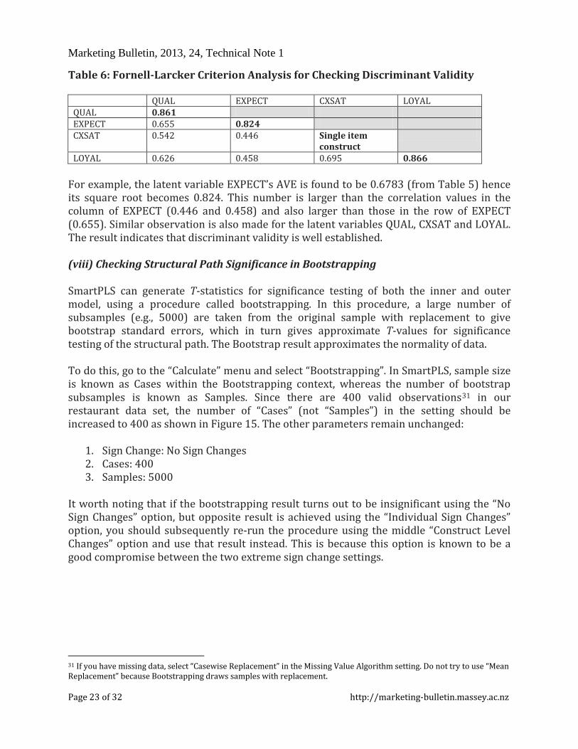
Table 6: Fornell-Larcker Criterion Analysis for Checking Discriminant Validity

QUAL EXPECT CXSAT LOYAL QUAL 0.861 EXPECT 0.655 0.824 CXSAT 0.542 0.446 Single item

construct

LOYAL 0.626 0.458 0.695 0.866 For example, the latent variable EXPECT’s AVE is found to be 0.6783 (from Table 5) hence its square root becomes 0.824. This number is larger than the correlation values in the column of EXPECT (0.446 and 0.458) and also larger than those in the row of EXPECT (0.655). Similar observation is also made for the latent variables QUAL, CXSAT and LOYAL. The result indicates that discriminant validity is well established. (viii) Checking Structural Path Significance in Bootstrapping SmartPLS can generate T-statistics for significance testing of both the inner and outer model, using a procedure called bootstrapping. In this procedure, a large number of subsamples (e.g., 5000) are taken from the original sample with replacement to give bootstrap standard errors, which in turn gives approximate T-values for significance testing of the structural path. The Bootstrap result approximates the normality of data. To do this, go to the “Calculate” menu and select “Bootstrapping”. In SmartPLS, sample size is known as Cases within the Bootstrapping context, whereas the number of bootstrap subsamples is known as Samples. Since there are 400 valid observations31 in our restaurant data set, the number of “Cases” (not “Samples”) in the setting should be increased to 400 as shown in Figure 15. The other parameters remain unchanged:

1. Sign Change: No Sign Changes 2. Cases: 400 3. Samples: 5000

It worth noting that if the bootstrapping result turns out to be insignificant using the “No Sign Changes” option, but opposite result is achieved using the “Individual Sign Changes” option, you should subsequently re-run the procedure using the middle “Construct Level Changes” option and use that result instead. This is because this option is known to be a good compromise between the two extreme sign change settings.

31 If you have missing data, select “Casewise Replacement” in the Missing Value Algorithm setting. Do not try to use “Mean Replacement” because Bootstrapping draws samples with replacement.



Figure 15: Bootstrapping Algorithm

Once the bootstrapping procedure is completed, go to the “Path Coefficients (Mean, STDEV, T-Values) window located within the Bootstrapping section of the Default Report. Check the numbers in the “T-Statistics” column to see if the path coefficients of the inner model are significant or not. Using a two-tailed t-test with a significance level of 5%, the path coefficient will be significant if the T-statistics32 is larger than 1.96. In our restaurant example, it can be seen that only the “EXPECT – LOYAL” linkage (0.0481) is not significant. This confirms our earlier findings when looking at the PLS-SEM results visually (see Figure 10). All other path coefficients in the inner model are statistically significant (see Figure 16 and Table 7)

32 The critical t-value is 1.65 for a significance level of 10%, and 2.58 for a significance level of 1% (all two-tailed)



Figure 16: Bootstrapping Results - Path Coefficients for Inner Model

Table 7: T-Statistics of Path Coefficients (Inner Model)

T-Statistics CXSAT LOYAL 12.2389 EXPECT CXSAT 2.5909 EXPECT LOYAL 0.0481 QUAL CXSAT 7.5904 QUAL LOYAL 6.6731

After reviewing the path coefficient for the inner model, we can explore the outer model by checking the T-statistic in the “Outer Loadings (Means, STDEV, T-Values)” window. As presented in table 8, all of the T-Statistics are larger than 1.96 so we can say that the outer model loadings are highly significant. All of these results complete a basic analysis of PLS-SEM in our restaurant example.



Table 8: T-Statistics of Outer Loadings

QUAL EXPECT CXSAT LOYAL qual_1 57.5315 qual_2 55.2478 qual_3 37.0593 expect_1 42.7139 expect_2 32.4697 expect_3 28.9727 cxsat Single item

construct

loyal_1 36.3623 loyal_2 97.6560 loyal_3 39.1145

Other Considerations When Conducting an In-depth Analysis of PLS-SEM The depth of the PLS-SEM analyze depends on the scope of the research project, the complexity of the model, and common presentation in prior literature. For example, a detailed PLS-SEM analysis would often include a multicollinearity assessment. That is, each set of exogenous latent variables in the inner model33 is checked for potential collinearity problem to see if any variables should be eliminated, merged into one, or simply have a higher-order latent variable developed. To assess collinearity issues of the inner model, the latent variable scores (PLS Calculation Results Latent Variable Scores) can be used as input for multiple regression in IBM SPSS Statistics to get the tolerance or Variance Inflation Factor (VIF) values, as SmartPLS does not provide these numbers. First, make sure the data set is in .csv file format. Then, import the data into SPSS and go to Analyze Regression Linear. In the linear regression module of SPSS, the exogenous latent variables (the predictors) are configured as independent variables, whereas another latent variable (which does not act as a predictor) is configured as the dependent variable. VIF is calculated as “1/Tolerance”. As a rule of thumb, we need to have a VIF of 5 or lower (i.e., Tolerance level of 0.2 or higher) to avoid the collinearity problem (Hair et al., 2011). In addition to checking collinearity, there can be a detailed discussion of the model’s f2

effect size34 which shows how much an exogenous latent variable contributes to an endogenous latent variable’s R2 value. In simple terms, effect size assesses the magnitude or strength of relationship between the latent variables. Such discussion can be important because effect size helps researchers to assess the overall contribution of a research study. Chin, Marcolin, and Newsted (1996) have clearly pointed out that researcher should not only indicate whether the relationship between variables is significant or not, but also report the effect size between these variables.

33 Also see the collinearity discussion for formative measurement model later in the paper for an example. 34 Effect size of 0.02, 0.15, and 0.35 indicates small, medium, and large effect, respectively.



Meanwhile, predictive relevance is another aspect that can be explored for the inner model. The Stone-Geisser’s (Q2) values35 (i.e., cross-validated redundancy measures) can be obtained by the Bindfolding procedure in SmartPLS (Calculate Bindfolding). In the Bindfolding setting window, an omission distance (OD) of 5 to 10 is suggested for most research (Hair et al., 2012). The q2 effect size for the Q2 values can also be computed and discussed. If a mediating latent variable exists in the model, one can also discuss the Total Effect of a particular exogenous latent variable on the endogenous latent variable. Total Effect value can be found in the default report (PLS Quality Criteria Total Effects). The significance of Total Effect can be tested using the T-Statistics in the Bootstrapping procedure (Bootstrapping Total Effects (Mean, STDEV, T-Values)). Also, unobserved heterogeneity may have to be assessed when there is little information about the underlying data, as it may affect the validity of PLS-SEM estimation. Managerial Implications - Restaurant Example The purpose of this example is to demonstrate how a restaurant manager can improve his/her business by understanding the relationships among customer expectation (EXPECT), perceived quality (QUAL), customer satisfaction (SAT) and customer loyalty (LOYAL). Through a survey of the restaurant patrons and the subsequent structural equation modeling in SmartPLS, the important factors that lead to customer loyalty are identified. In this research, customers are found to care about food taste, table service, and bill accuracy. With loadings of 0.881, 0.873 and 0.828 respectively, they are good indicators of perceived quality (QUAL). Restaurant management should not overlook these basic elements of day-to-day operation because perceived quality has been shown to significantly influence customers’ satisfaction level, their intention to come back, and whether or not they would recommend this restaurant to others. Meanwhile, it is also revealed that menu selection, atmospheric elements and good-looking staff are important indicators of customer expectation (EXPECT), with loadings of 0.848, 0.807, and 0.816 respectively. Although fulfilling these customer expectations can keep them satisfied, improvement in these areas does not significantly impact customer loyalty due to its weak effect (0.03) in the linkage. As a result, management should only allocate resources to improve these areas after food taste, table service and bill accuracy have been looked after. The analysis of inner model shows that perceived quality (QUAL) and customer expectation (EXPECT) together can only explain 30.8% of the variance in customer satisfaction (CXSAT). It is an important finding because it suggests that there are other factors that

35. Q2 values of 0.02, 0.15 and 0.35 indicate an exogenous construct has a small, medium and large predictive relevance for an endogenous latent variable respectively.



restaurant managers should consider when exploring customer satisfaction in future research. Assessing Formative Measurement Model As described earlier in this paper, a model does not necessarily have reflective measurements. When working with a formative measurement model, we do not analyze indicator reliability, internal consistency reliability, or discriminant validity because the formative indicators are not highly correlated together. Instead, we analyze the model’s outer weight (not outer loadings!), convergent validity, and collinearity of indicators. Outer model weight and significance For formative measurement models, the outer weights can be found using the path (PLS Calculation Results Outer Weight) after the PLS algorithm is run. Marketers should pay attention to those indicators with high outer weights as they are the important area or aspect of the business that should be focused on. In SmartPLS, bootstrapping can also be used to test the significance of formative indicators’ outer weight. After running the procedure, check the T-Statistics value as shown in the “Outer Weights” window (Bootstrapping Bootstrapping Outer Weights [Mean, STDEV, T-Values]). If a particular indicator’s outer weight is shown as not significant (i.e., <1.96), check the significance of its outer loading. Only remove the indicator if both of its outer weights and outer loadings are not significant.

Convergent validity

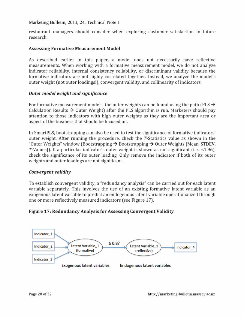
To establish convergent validity, a “redundancy analysis” can be carried out for each latent variable separately. This involves the use of an existing formative latent variable as an exogenous latent variable to predict an endogenous latent variable operationalized through one or more reflectively measured indicators (see Figure 17). Figure 17: Redundancy Analysis for Assessing Convergent Validity



The reflective indicator (“Indicator_4” as in Figure 17) can be a global item in the questionnaire that summarizes the essence of the latent variable the formative indicators (“Indicator_1”, “Indicator_2”, and “Indicator_3”) intend to measure. For example, if the “Latent Variable_1” is about Corporate Social Responsibility, a survey question such as “Please evaluate to what degree this organization acted in a socially responsible way?” can be asked on a Likert scale of 0 (not a all) to 7 (completely), and this is the data for “Indicator_4”. To do this in SmartPLS, a new model has to be built for each latent variable as in figure 15 for PLS-SEM testing. When the correlation (path coefficient) between the latent variables is 0.80 or higher, convergent validity is established (Hair et al., 2013).

Collinearity of Indicators In a formative measurement model, the problem of indicator collinearity may occur if the indicators are highly correlated to each other. As discussed earlier in the paper, multiple regression in SPSS can be used to generate VIF and Tolerance values for collinearity checking. The formative indicators of a latent variable are set as independent variables, with the indicator of another latent variable as dependent variable. In the “Statistics..” window, check “Estimates”, “Model Fit” and “Collinearity diagnostics”. Once the linear regression is run, locate the “Coefficients” table in the SPSS Output. Only the Tolerance and VIF values showing in the “Collinearity Statistics” column are needed for this collinearity analysis. See Figure 18 for an example. Figure 18: Tolerance and VIF values in SPSS Output

Looking at a fictitious example as shown in Figure 18, all of the indicators’ VIF values are lower than 5 and their Tolerance values are higher than 0.2, so there is no collinearity problem. Model with Both Reflective and Formative Measurements It is important to note that in some research projects, both reflective and formative measurements are present in the same model. In other words, some latent variables have



arrows pointing away from them, whereas there are also latent variables that have arrows pointing to them from their indicators. If this is the case, analysis should be carried out separately for each part of the model. Outer loadings and outer weights have to be examined carefully for reflective and formative indicators respectively. Conclusion This paper has discussed the use of a second-generation multivariate data analysis method called Structural Equation Modeling (SEM) for consumer research, with a focus on Partial Least Squares (PLS) which is an emerging path modeling approach. A simulated restaurant example is presented using the SmartPLS software to help marketers master the basics of PLS-SEM quickly in a step-by-step manner. This Technical Note only serves as a quick start guide to the SmartPLS software for beginners. Advanced users who want to explore the field of PLS-SEM further can refer to the works of Esposito Vinzi et al. (2010) and Hair et al. (2013). References Bacon, L. D. (1999). Using LISREL and PLS to Measure Customer Satisfaction, Sawtooth

Software Conference Proceedings, La Jolla, California, Feb 2-5, 305-306. Bagozzi, R. P., & Yi, Y. (1988). On the evaluation of structural equation models. Journal of

the Academy of Marketing Science, 16(1), 74–94. Bass, B., Avolio, B., Jung, D., & Berson Y. (2003). Predicting unit performance by assessing

transformational and transactional leadership. Journal of Applied Psychology 88(2), 207–218.

Chin, W. W. (1998). The partial least squares approach to structural equation modeling. In

G. A. Marcoulides (Ed.), Modern methods for business research (295–336). Mahwah, New Jersey: Lawrence Erlbaum Associates.

Chin, W. W., Marcolin, B. L., & Newsted, P. R. (1996). A partial least squares latent variable

modelling approach for measuring interaction effects: Results from a Monte Carlo simulation study and voice mail emotion/adoption study. Paper presented at the 17th International Conference on Information Systems, Cleveland, OH.

Chin, W. W., Marcolin, B. L., & Newsted, P. R (2003). A Partial Least Squares Latent Variable

Modeling Approach For Measuring Interaction Effects: Results From A Monte Carlo Simulation Study And Electronic Mail Emotion/Adoption Study, Information Systems Research, 14(2), 189-217.

Cohen, J. (1992). A power primer. Psychological Bulletin, 112(1), 155-159.



Esposito Vinzi V., Trinchera L., Squillacciotti S., & Tenenhaus M. (2008). REBUSPLS: A response-based procedure for detecting unit segments in PLS path modeling,

Applied Stochastic Models in Business and Industry, 24(5), 439-458. Esposito Vinzi, V., Trinchera, L., & Amato, S. (2010). PLS Path Modeling: From Foundations

to Recent Developments and Open Issues for Model Assessment and Improvement. In. V. Esposito Vinzi, W.W. Chin, J. Henseler & H. Wang (Eds) Handbook of Partial Least Squares: Concepts, Methods and Applications (47-82) Berlin, Germany: Springer Berlin Heidelberg

Fornell, C., & Larcker, D.F., (1981). Evaluating structural equation models with

unobservable variables and measurement error. Journal of Marketing Research, 18 (1), 39-50.

Frank, B. & Hennig-Thurau, T. (2008). Identifying hidden structures in marketing’s

structural models through Universal Structure Modeling: An explorative Bayesian Neural Network complement to LISREL and PLS', Marketing -- Journal of Research and Management, 4(2), 47-66.

Haenlein, M. & Kaplan, A. M. (2004). A beginner’s guide to partial least squares analysis,

Understanding Statistics, 3(4), 283–297. Hair, J. F., Black, W. C., Babin, B. J., & Anderson, R. E. (2010). Multivariate data analysis (7th

ed.). Englewood Cliffs: Prentice Hall Hair, J. F., Hult, G. T. M., Ringle, C. M., & Sarstedt, M. (2013). A Primer on Partial Least

Squares Structural Equation Modeling (PLS-SEM). Thousand Oaks: Sage. Hair, J. F., Ringle, C. M., & Sarstedt, M. (2011). PLS-SEM: Indeed a silver bullet. Journal of

Marketing Theory and Practice, 19(2), 139–151. Hair, J.F., Sarstedt, M., Ringle, C.M. & Mena, J.A., (2012). An assessment of the use of partial

least squares structural equation modeling in marketing research. Journal of the Academy of Marketing Science, 40(3), 414-433.

Henseler, J. (2010). On the convergence of the partial least squares path modeling

algorithm. Computational Statistics, 25(1), 107–120. Henseler. J. and Sarstedt, M. (2013). Goodness-of-fit indices for partial least squares path

modeling. Computational Statistics. 28 (2), 565-580. Henseler, J., Ringle, C., & Sinkovics, R. (2009). The use of partial least squares path modeling

in international marketing. Advances in International Marketing, 20(2009), 277–320. Hoyle, R. H. (ed.) (1995). Structural Equation Modeling. Thousand Oaks, CA.: SAGE

Publications, Inc.



Hulland, J. (1999). Use of partial least squares (PLS) in strategic management research: a

review of four recent studies. Strategic Management Journal, 20(2), 195–204. Hwang, H., Malhotra, N. K., Kim, Y., Tomiuk, M. A., & Hong, S. (2010). A comparative study

on parameter recovery of three approaches to structural equation modeling. Journal of Marketing Research, 47 (Aug), 699-712.

Marcoulides, G. A., & Saunders, C. (2006, June). Editor’s Comments – PLS: A Silver Bullet?

MIS Quarterly, 30(2), iii-ix. Petter, S., Straub, D., and Rai, A. (2007). Specifying formative constructs in information

systems research, MIS Quarterly, 31 (4), 623-656. Reinartz, W.J., Haenlein, M & Henseler, J. (2009). An empirical comparison of the efficacy

of covariance-based and variance-based SEM,” International Journal of Market Research, 26 (4), 332–344.

Ringle, C., Wende, S., & Will, A. (2005). SmartPLS 2.0 (Beta). Hamburg, (www.smartpls.de). Sosik J J, Kahai S S, Piovoso M J (2009) Silver bullet or voodoo statistics? A primer for using

the partial least squares data analytic technique in group and organization research. Emerald Management Reviews: Group & Organization Management, 34(1), 5-36.

Statsoft (2013). Structural Equation Modeling, Statsoft Electronic Statistics Textbook.

http://www.statsoft.com/textbook/structural-equation-modeling/ Wold, H. (1973). Nonlinear Iterative Partial Least Squares (NIPALS) Modeling: Some

Current Developments, in Paruchuri R. Krishnaiah (Ed.), Multivariate Analysis (Vol. 3, pp. 383-407). New York: Academic Press.

Wold, H. (1985). Partial Least Squares. In S. Kotz & N. L. Johnson (Eds.), Encyclopedia of

Statistical Sciences (Vol. 6, pp. 581–591). New York: John Wiley & Sons. Wong, K. K. (2010). Handling small survey sample size and skewed dataset with partial

least square path modelling. Vue: The Magazine of the Marketing Research and Intelligence Association, November, 20-23.

Wong, K. K. (2011). Review of the book Handbook of Partial Least Squares: Concepts,

Methods and Applications, by V. Esposito Vinzi, W.W. Chin, J. Henseler & H. Wang (Eds). International Journal of Business Science & Applied Management. 6 (2), 52-54.

Acknowledgements: The author would like to acknowledge his gratitude to Professor Donna Smith (Ryerson University, Canada), and also the journal’s peer reviewers, whose comments resulted in a notable improvement of this article. Dr. Ken Kwong-Kay Wong is an Assistant Professor of Retail Management at the Ted Rogers School of Management, Ryerson University. ([email protected])


Partial Least Squares Structural Equation Modeling...

Documents

Transcript of Partial Least Squares Structural Equation Modeling...