A Partial Least Squares based algorithm for parsimonious variable

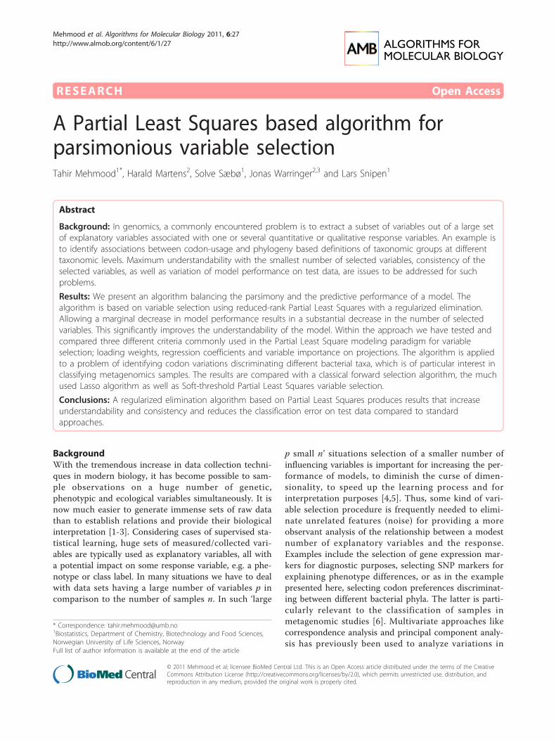
RESEARCH Open Access

A Partial Least Squares based algorithm forparsimonious variable selectionTahir Mehmood1*, Harald Martens2, Solve Sæbø1, Jonas Warringer2,3 and Lars Snipen1

Abstract

Background: In genomics, a commonly encountered problem is to extract a subset of variables out of a large setof explanatory variables associated with one or several quantitative or qualitative response variables. An example isto identify associations between codon-usage and phylogeny based definitions of taxonomic groups at differenttaxonomic levels. Maximum understandability with the smallest number of selected variables, consistency of theselected variables, as well as variation of model performance on test data, are issues to be addressed for suchproblems.

Results: We present an algorithm balancing the parsimony and the predictive performance of a model. Thealgorithm is based on variable selection using reduced-rank Partial Least Squares with a regularized elimination.Allowing a marginal decrease in model performance results in a substantial decrease in the number of selectedvariables. This significantly improves the understandability of the model. Within the approach we have tested andcompared three different criteria commonly used in the Partial Least Square modeling paradigm for variableselection; loading weights, regression coefficients and variable importance on projections. The algorithm is appliedto a problem of identifying codon variations discriminating different bacterial taxa, which is of particular interest inclassifying metagenomics samples. The results are compared with a classical forward selection algorithm, the muchused Lasso algorithm as well as Soft-threshold Partial Least Squares variable selection.

Conclusions: A regularized elimination algorithm based on Partial Least Squares produces results that increaseunderstandability and consistency and reduces the classification error on test data compared to standardapproaches.

BackgroundWith the tremendous increase in data collection techni-ques in modern biology, it has become possible to sam-ple observations on a huge number of genetic,phenotypic and ecological variables simultaneously. It isnow much easier to generate immense sets of raw datathan to establish relations and provide their biologicalinterpretation [1-3]. Considering cases of supervised sta-tistical learning, huge sets of measured/collected vari-ables are typically used as explanatory variables, all witha potential impact on some response variable, e.g. a phe-notype or class label. In many situations we have to dealwith data sets having a large number of variables p incomparison to the number of samples n. In such ‘large

p small n’ situations selection of a smaller number ofinfluencing variables is important for increasing the per-formance of models, to diminish the curse of dimen-sionality, to speed up the learning process and forinterpretation purposes [4,5]. Thus, some kind of vari-able selection procedure is frequently needed to elimi-nate unrelated features (noise) for providing a moreobservant analysis of the relationship between a modestnumber of explanatory variables and the response.Examples include the selection of gene expression mar-kers for diagnostic purposes, selecting SNP markers forexplaining phenotype differences, or as in the examplepresented here, selecting codon preferences discriminat-ing between different bacterial phyla. The latter is parti-cularly relevant to the classification of samples inmetagenomic studies [6]. Multivariate approaches likecorrespondence analysis and principal component analy-sis has previously been used to analyze variations in

* Correspondence: [email protected], Department of Chemistry, Biotechnology and Food Sciences,Norwegian University of Life Sciences, NorwayFull list of author information is available at the end of the article

Mehmood et al. Algorithms for Molecular Biology 2011, 6:27http://www.almob.org/content/6/1/27

© 2011 Mehmood et al; licensee BioMed Central Ltd. This is an Open Access article distributed under the terms of the CreativeCommons Attribution License (http://creativecommons.org/licenses/by/2.0), which permits unrestricted use, distribution, andreproduction in any medium, provided the original work is properly cited.

mailto:[email protected]

http://creativecommons.org/licenses/by/2.0

codon usage among genes [7]. However, in order torelate the selection specifically to a response vector, likethe phylum assignment, we need a selection based on asupervised learning method.Partial Least Square (PLS) regression is a supervised

method specifically established to address the problemof making good predictions in the ‘large p small n’ situa-tion, see [8]. PLS in its original form has no implemen-tation of variable selection, since the focus of themethod is to find the relevant linear subspace of theexplanatory variables, not the variables themselves.However, a very large p and small n can spoil the PLSregression results, as demonstrated by Keles et. al. [9],discovering that the asymptotic consistency of the PLSestimators for univariate responses do not hold, and by[10], who observed a large variation on test set.Boulesteix has theoretically explored a tight connec-

tion between PLS dimension reduction and variableselection [11] and work in this field has existed formany years. Examples are [8,9,11-23]. For an optimumextraction of a set of variables, we need to look for allpossible subsets of variables, which is impossible if p islarge enough. Normally a set of variables with a reason-able performance is a compromise over the optimal subset.In general, variable selection procedures can be cate-

gorized [5] into two main groups: filter methods andwrapper methods. Filter methods select variables as apreprocessing step independently of some classifier orprediction model, while wrapper methods are based onsome supervised learning approach [12]. Hence, anyPLS-based variable selection is a wrapper method.Wrapper methods need some sort of criterion that reliessolely on the characteristics of the data as described by[5,12]. One candidate among these criteria is thePLS loading weights, where down-weighting smallPLS loading weights is used for variable selection[8,11,13-17,24-27]. A second possibility is to use themagnitude of the PLS regression coefficients for variableselection [18-20,28-34]. Jackknifing and/or bootstrappingon regression coefficients has been utilized to selectinfluencing variables [20,30,31,33,34]. A third commonlyused criterion is the Variables Importance on PLS pro-jections (VIP) introduced by Eriksson et. al. [21] and iscommonly used in practise [22,31,35-37].There are several PLS-based wrapper selection algo-

rithms, for example uninformative variable elimination(UVE-PLS) [18], where artificial random variables areadded to the data as a reference such that the variablewith least performance are eliminated. Iterative PLS(IPLS) adds new variable(s) in the model or removevariables from the model if it improves the model per-formance [19]. A backward elimination procedure based

on leave one variable out is another example [5].Although wrapper based methods perform well thenumber of variables selected is still often large [5,12,38],which may make interpretation hard ([23,39,40]).Among recent advancements in PLS methodology

itself we find that Indahl et. al. [41] propose a new datacompression method for estimating optimal latent vari-ables classification and regression problems by combin-ing PLS methodology and canonical correlation analysis(CCA), called Canonical Powered PLS (CPPLS). In ourwork we have adopted this new methodology and pro-posed a regularized greedy algorithm based on a back-ward elimination procedure. The focus is onclassification problems, but the same concept can beused for prediction problems as well. Our principle ideais to focus on a parsimonious selection, achieved by tol-erating a minor performance deviation from any ‘opti-mum’ if this gives a substantial decrease in the numberof selected variables. This is implemented as a regulari-zation of the search for optimum performance, makingthe selection less dependent on ‘peak performance’ andhence more stable. In this respect, the choice of theCPPLS variant is not important, and even the use ofnon-PLS based methods could in principle be imple-mented with some minor adjustments. Both loadingweights, PLS regression coefficients significance obtainedfrom jackknifing and VIP are explored here for orderingthe variables with respect to their importance.

1 Methods1.1 Model fittingWe consider a classification problem where every objectbelongs to one out of two possible classes, as indicatedby the n × 1 class label vector C. From C we create then × 1 numeric response vector y by dummy coding, i.e.y contains only 0’s and 1’s. The association between yand the n × p predictor matrix X is assumed to beexplained by the linear model E(y) = Xb where b are thep × 1 vector of regression coefficients. The purpose ofvariable selection is to find a column subset of X cap-able of satisfactory explaining the variations in C.From a modeling perspective, ordinary least square fit-

ting is no option when n <p. PLS resolves this bysearching for a small set of components, ‘latent vectors’,that performs a simultaneous decomposition of X and ywith the constraint that these components explain asmuch as possible of the covariance between X and y.

1.2 Canonical Powered PLS (CPPLS) RegressionPLS is an iterative procedure where relation between Xand y is found through the latent variables. The PLSestimate of the regression coefficients for the abovegiven model based on k components can be achieved by


of 12

β = W(P′1W)−1p′

2 (1)

where P1 is the pl × k matrix of X-loadings that issummary of X-variables, p2 is the a vector of y-loadingsi.e. summary of y-variables and W is the p × k matrix ofloading weights, for details see [8]. Recently, Indahl et.al. [41] proposed a new data compression method forestimating optimal latent variables by combining PLSmethodology and canonical correlation analysis (CCA).They introduce a flexible trade-off between the elementwise correlations and variances specified by a powerparameter g, ranging from 0 to 1. Defines the loadingweights as

w(γ ) = Kγ

⎡⎣s1|corr(x1, y)|

γ

1 − γ .std(x1)

1 − γ

γ , ...,

sp|corr(xp, y)|γ

1 − γ .std(xp)

1 − γ

γ

⎤⎥⎦

t

where sk denotes the sign of the kth correlation and Kg

is a scaling constant assuring unit length w(g). In thisstudy we restricted g to lower region (0.001, 0.050) andto upper region (0.950, 0.999). This means we considercombinations of g for emphasizing either the variance (gclose to 0) or the correlations (g close to 1). The g valuefrom above regions that optimizes the canonical correla-tion is always selected for each component of CPPLSalgorithm, see Indahl et. al. [41] for details on theCPPLS algorithm.Based on the CPPLS estimated regression coefficients

β we can predict the dummy-variables by

y = Xβ

and from the data set (y,C) we build a classifier usingstraightforward linear discriminant analysis [42].

1.3 First regularization - model dimension estimateThe CPPLS algorithm assumes that the column space ofX has a subspace of dimension a containing all informa-tion relevant for predicting y (known as the relevantsubspace) [43]. In order to estimate a we use cross-vali-dation and the performance Pa defined as the fraction ofcorrectly classified observations in a cross-validationprocedure, using a components in the CPPLS algorithm.The cross-validation estimate of a can be found by

systematically trying out a range of dimensions a = 1,...,A, compute Pa for each a, and choose as α the a wherewe reach the maximum Pa. Let us denote this value a*.It is well known that in many cases Pa will be almostequally large for many choices of a. Thus, estimating aby this maximum value is likely to be a rather unstableestimator. To stabilize this estimate we use a regulariza-tion based on the principle of parsimony where we

search for the smallest possible a whose correspondingperformance is not significantly worse than the opti-mum. If ra is the probability of a correct classificationusing the a-component model, and ra* similar for thea*-component model, we test H0 : ra = ra* against thealternative H1 : ra <ra*. In practice Pa and Pa* are esti-mates of ra and ra*. The smallest a where we cannotreject H0 is our estimate α. The testing is done by ana-lyzing the 2 × 2 contingency table of correct and incor-rect classifications for the two choices of a, using theMcNemar test [44]. This test is appropriate since themodel classification at a specific component depends onthe model classification at the other components.This regularization depends on a user-defined rejec-

tion level c of the McNemar test. Using a large c (closeto 1) means we easily reject H0, and the estimate α isoften similar to a*. By choosing a smaller c (closer to 0)we get a harder regularization, i.e. a smaller α and morestability at the cost of a lower performance.

1.4 Selection criteriaWe have implemented and tried out three different cri-teria for PLS-based variable selection:1.4.1 Loading weightsVariable j can be eliminated if the relative loadingweight, rj for a given PLS component satisfies

rj = | wa,j

maxwa| < u for some chosen threshold u Î [0, 1].

1.4.2 Regression coefficientsVariable j can be eliminated if the corresponding regres-sion coefficient bj = 0. Testing H0 : bj = 0 against H1: bj≠ = 0 can be done by a jackknife t-test. All computa-tions needed have already been done in the cross-valida-tion used for estimating the model dimension a. Foreach variable we compute the corresponding false dis-covery rate (q -value) which is based on the p valuesfrom jackknifing, and variable j can be eliminated if qj>u for some fixed threshold u Î [0, 1].1.4.3 Variable importance on PLS projections (VIP)VIP for the variable j is defined according to [21] as

vj =

√√√√pa∗∑a=1

[(p22at′ata)(waj/||wa||)2]/

a∗∑a=1

(p22a(t′ata)

where a = 1, 2, ..., a*, waj is the loading weight forvariable j using a components and ta, wa and p2a areCPPLS scores, loading weights and y-loadings respec-tively corresponding to the ath component. [22] explainsthe main difference between the regression coefficient bjand vj. The vj weights the contribution of each variableaccording to the variance explained by each PLS compo-nent, i.e. p22at

′ata where (waj/||wa||)

2 represents theimportance of the jth variable. Variable j can be


of 12

eliminated if vj <u for some user-defined threshold u Î[0, ∞). It is generally accepted that a variable shouldbe selected if vj > 1, see [21,22,36], but a proper thresh-old between 0.83 and 1.21 can maximize the perfor-mance [36].

1.5 Backward eliminationWhen we have n <<p it is very difficult to find the trulyinfluencing variables since the estimated relevant sub-space found by Cross-Validated CPPLS (CVCPPLS) isbound to be, to some degree, ‘infested’ by non-influen-cing variables. This may easily lead to errors both ways,i.e. both false positives and false negatives. An approachto improve on this is to implement a stepwise estima-tion where we gradually eliminate ‘the worst’ variablesin a greedy algorithm.The algorithm can be sketched as follows: Let Z0 = X

and let sj be one of the criteria for variable j we havesketched above (either rj, qj or vj).

1) For iteration g run y and Zg through CVCPPLS.The matrix Zg has pg columns, and we get the samenumber of criterion values, sorted in ascendingorder as s(1), ..., s(pg).2) There are M criterion values below (above forciterion qj) the cutoff u. If M = 0, terminate thealgorithm here.3) Else, let N = ⌈fM⌉ for some fraction f Î ⟨0,1].Eliminate the variables corresponding to the N mostextreme criterion values.4) If there are still more than one variable left, let Zg

+1 contain these variables, and return to 1).

The fraction f determines the ‘steplength’ of the elimi-nation algorithm, where an f close to 0 will only elimi-nate a few variables in every iteration. The fraction fand u can be obtained through cross validation.

1.6 Second regularization - final selectionIn each iteration of the elimination the CVCPPLS algo-rithm computes the cross-validated performance, andwe denote this with Pg for iteration g. After each itera-tion, the number of influencing variables decreases, butPg will often increase until some optimum is achieved,and then drop again as we keep on eliminating. Theinitial elimination of variables stabilizes the estimates ofthe relevant subspace in the CVCPPLS algorithm, andhence we get an increase in performance. Then, if theelimination is too severe, we start to lose informativevariables, and even if stability is increased even more,the performance drops.

Let the optimal performance be defined as

P∗ = Pg∗ = maxg

Pg

It is not unreasonable to use the variables still presentafter iteration g* as the final selected variables. This iswhere we have achieved a balance between removingnoise and keeping informative variables. However, fre-quently we observe that a severe reduction in the num-ber variables compared to this ‘optimum’ will give onlya modest drop in performance. Hence, we may eliminatewell beyond g*, and find a much simpler model, at asmall loss in performance. To formalize this, we useexactly the same procedure, involving the McNemar testthat we used in the regularization of the model dimen-sion estimate. If rg is the probability of a correct classifi-cation after g iterations, and rg* similar after g*iterations, we test H0 : rg = rg* against the alternativeH1 : rg <rg*. The largest g where we cannot reject H0 isthe iteration where we find our final selected variables.This means we need another rejection level d which willdecide to which degree we are willing to sacrifice perfor-mance over a simpler model. Using d close to 0 meanswe emphasize simplicity over performance. In practice,for each iteration beyond g* we can compute the McNe-mar test p-value, and list this together with the numberof variables remaining, to give a perspective on thetrade-off between understandability of the model andthe performance. Figure 1 presents the procedure in aflow chart.

1.7 Choices of variable selection methods for comparisonThree variable selection methods are also considered forcomparison purposes. The classical forward selection

Z0 = X

CVCPPLS (y Zg) ‘c’ significance level of regularization

s(1) , ... , s(M), s(M+1), ... , s(pg)

M s-values above cutoff ‘u’ STOP if M=0

Eliminate N=[fM] s-values STOP if no variable left

Zg+1

Figure 1 Flow chart. The flow chart illustrates the proposedalgorithm for variable selection.


of 12

procedure (Forward) is a univariate approach, and prob-ably the simplest approach to variable selection for the‘large p small n’ type of problems considered here. TheLeast Absolute Shrinkage and Selection Operator(Lasso) [45] is a method frequently used in genomics.Recent examples are the extraction of molecular signa-tures [46] and gene selection from microarrays [47]. TheSoft-Thresholding PLS (ST-PLS) [17] implements theLasso concept in a PLS framework. A recent applicationof ST-PLS is the mapping of genotype to phenotypeinformation [48].All methods are implemented in the R computing

environment http://www.r-project.org/.

2 ApplicationAn application of the variable selection procedure is tofind the preferred codons associated with certain pro-karyotic phyla.Codons are triplets of nucleotides in coding genes and

the messenger RNA; these triplets are recognized bybase-pairing by corresponding anticodons on specifictransfer RNA carrying individual amino acids. This facil-itates the translation of genetic messenger informationinto specific proteins. In the standard genetic code, the20 amino acids are individually coded by 1, 2, 4 or 6 dif-ferent codons (excluding the three stop codons there are61 codons). However, the different codons encodingindividual amino acids are not selectively equivalentbecause the corresponding tRNAs differ in abundance,allowing for selection on codon usage. Codon preferenceis considered as an indicator of the force shaping gen-ome evolution in prokaryotes [49,50], reflection of lifestyle [49] and organisms within similar ecological envir-onments often have similar codon usage pattern in theirgenomes [50,51]. Higher order codon frequencies, e.g.di-codons, are considered important with respect tojoint effects, like synergistic effect, of codons [52].There are many suggested procedures to analyze

codon usage bias, for example the codon adaptationindex [53], the frequency of optimal codons [54] andthe effective number of codons [55]. In the currentstudy, we are not specifically looking at codon bias, buthow the overall usage of codons can be used to distin-guish prokaryote phyla. Notice that the overall codonusage is affected both by the selection of amino acidsand codon bias within the redundant amino acids. Phy-lum is a relevant taxonomic level for metagenomic stu-dies [56,57], so interest lies in having a systematicsearch for codon usage at the phylum level [58-60].

2.1 DataGenome sequences for 445 prokaryote genomes and therespective Phylum information were obtained fromNCBI Genome Projects (http://www.ncbi.nlm.nih.gov/

genomes/lproks.cgi). The response variable in our dataset is phylum, i.e. the highest level taxonomic classifierof each genome, in the bacterial kingdom. There are intotal 11 several phyla in our data set including Actino-bacteria, Bacteroides, Crenarchaeota, Cyanobac-teria,Euryarchaeota, Firmicutes, Alphaproteobacteria, Beta-proteobacteria, Deltaproteobacteria, Gammapro-teobac-teria and Epsilonproteobacteria. We only consider two-class problems, i.e. for some fixed ‘phylum A’, we onlyclassify genomes as either ‘phylum A’, or ‘not phylumA’. Thus, the data set has n = 445 samples and 11 dif-ferent responses of 0/1 outcome, considering one at atime.Genes for each genome were predicted by the gene-

finding software Prodigal [61], which uses dynamic pro-gramming in which start codon usage, ribosomal sitemotif usage and GC frame bias are considered for geneprediction. For each genome, we collected the frequen-cies of each codon and each di-codon over all genes.The predictor variables thus consists of relative frequen-cies for all codons and di-codons, giving a predictormatrix X with a total of p = 64 + 642 = 4160 variables(columns).

2.2 Parameter setting/tuningIt is in principle no problem to eliminate (almost) allvariables, since we always go back to the iteration wherewe cannot reject the null-hypothesis of the McNemartest. Hence, we fixed u at extreme values, 0.99 for load-ing weights, 0.01 for regression coefficients and 10 forVIP. Three levels of step length f = (0.1,0.5, 1) were con-sidered. In the first regularization step we tried threevery different rejection levels c = (0.1,0.5, 1) and in thesecond we used two extreme levels (d = (0.01,0.99)).

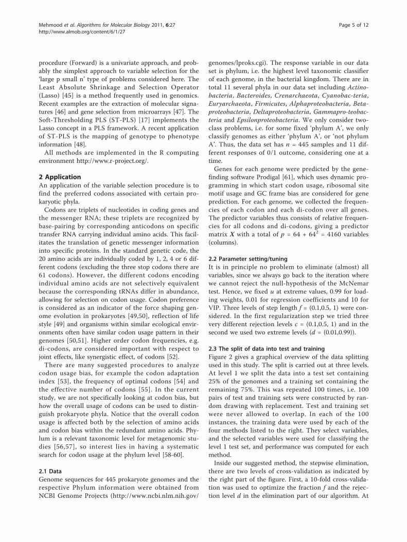
2.3 The split of data into test and trainingFigure 2 gives a graphical overview of the data splittingused in this study. The split is carried out at three levels.At level 1 we split the data into a test set containing25% of the genomes and a training set containing theremaining 75%. This was repeated 100 times, i.e. 100pairs of test and training sets were constructed by ran-dom drawing with replacement. Test and training setwere never allowed to overlap. In each of the 100instances, the training data were used by each of thefour methods listed to the right. They select variables,and the selected variables were used for classifying thelevel 1 test set, and performance was computed for eachmethod.Inside our suggested method, the stepwise elimination,

there are two levels of cross-validation as indicated bythe right part of the figure. First, a 10-fold cross-valida-tion was used to optimize the fraction f and the rejec-tion level d in the elimination part of our algorithm. At


of 12

http://www.r-project.org/

http://www.ncbi.nlm.nih.gov/genomes/lproks.cgi

http://www.ncbi.nlm.nih.gov/genomes/lproks.cgi

level 3 leave-one-out cross-validation was used to esti-mate all parameters in the regularized CPPLS method,including the rejection level c. These two levels togethercorresponds to a ‘cross-model validation’ [62].

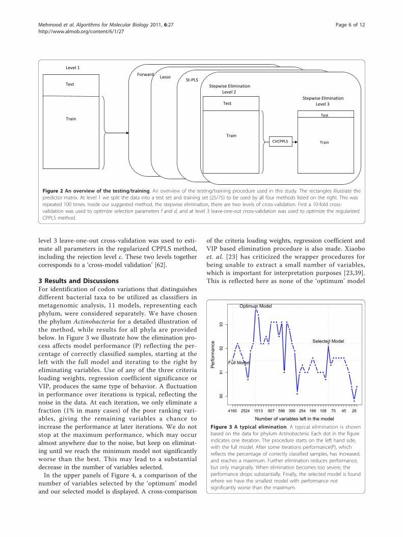
3 Results and DiscussionsFor identification of codon variations that distinguishesdifferent bacterial taxa to be utilized as classifiers inmetagenomic analysis, 11 models, representing eachphylum, were considered separately. We have chosenthe phylum Actinobacteria for a detailed illustration ofthe method, while results for all phyla are providedbelow. In Figure 3 we illustrate how the elimination pro-cess affects model performance (P) reflecting the per-centage of correctly classified samples, starting at theleft with the full model and iterating to the right byeliminating variables. Use of any of the three criterialoading weights, regression coefficient significance orVIP, produces the same type of behavior. A fluctuationin performance over iterations is typical, reflecting thenoise in the data. At each iteration, we only eliminate afraction (1% in many cases) of the poor ranking vari-ables, giving the remaining variables a chance toincrease the performance at later iterations. We do notstop at the maximum performance, which may occuralmost anywhere due to the noise, but keep on eliminat-ing until we reach the minimum model not significantlyworse than the best. This may lead to a substantialdecrease in the number of variables selected.In the upper panels of Figure 4, a comparison of the

number of variables selected by the ‘optimum’ modeland our selected model is displayed. A cross-comparison

of the criteria loading weights, regression coefficient andVIP based elimination procedure is also made. Xiaoboet. al. [23] has criticized the wrapper procedures forbeing unable to extract a small number of variables,which is important for interpretation purposes [23,39].This is reflected here as none of the ‘optimum’ model

Forward

Lasso

St-PLS

Level 1

Test

Train

Stepwise Elimination Level 2

Test

Train

Test

Train

CVCPPLS

Stepwise Elimination Level 3

Figure 2 An overview of the testing/training. An overview of the testing/training procedure used in this study. The rectangles illustrate thepredictor matrix. At level 1 we split the data into a test set and training set (25/75) to be used by all four methods listed on the right. This wasrepeated 100 times. Inside our suggested method, the stepwise elimination, there are two levels of cross-validation. First a 10-fold cross-validation was used to optimize selection parameters f and d, and at level 3 leave-one-out cross-validation was used to optimize the regularizedCPPLS method.

9091

9293

Number of variables left in the model

Perfo

rman

ce

4160 2524 1513 907 596 390 254 166 108 70 45 28

Full Model

Optimum Model

Selected Model

Figure 3 A typical elimination. A typical elimination is shownbased on the data for phylum Actinobacteria. Each dot in the figureindicates one iteration. The procedure starts on the left hand side,with the full model. After some iterations performance(P), whichreflects the percentage of correctly classified samples, has increased,and reaches a maximum. Further elimination reduces performance,but only marginally. When elimination becomes too severe, theperformance drops substantially. Finally, the selected model is foundwhere we have the smallest model with performance notsignificantly worse than the maximum.


of 12

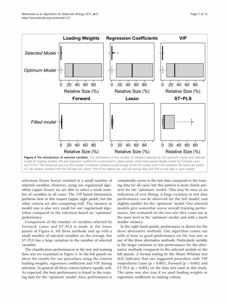
selections (lower boxes) resulted in a small number ofselected variables. However, using our regularized algo-rithm (upper boxes) we are able to select a small num-ber of variables in all cases. The VIP based eliminationperforms best in this respect (upper right panel), but theother criteria are also competing well. The variance inmodel size is also very small for our regularized algo-rithm compared to the selection based on ‘optimum’performance.Comparison of the number of variables selected by

Forward, Lasso and ST-PLS is made in the lowerpanels of Figure 4. All three methods end up with asmall number of selected variables on the average, butST-PLS has a large variation in the number of selectedvariables.The classification performances in the test and training

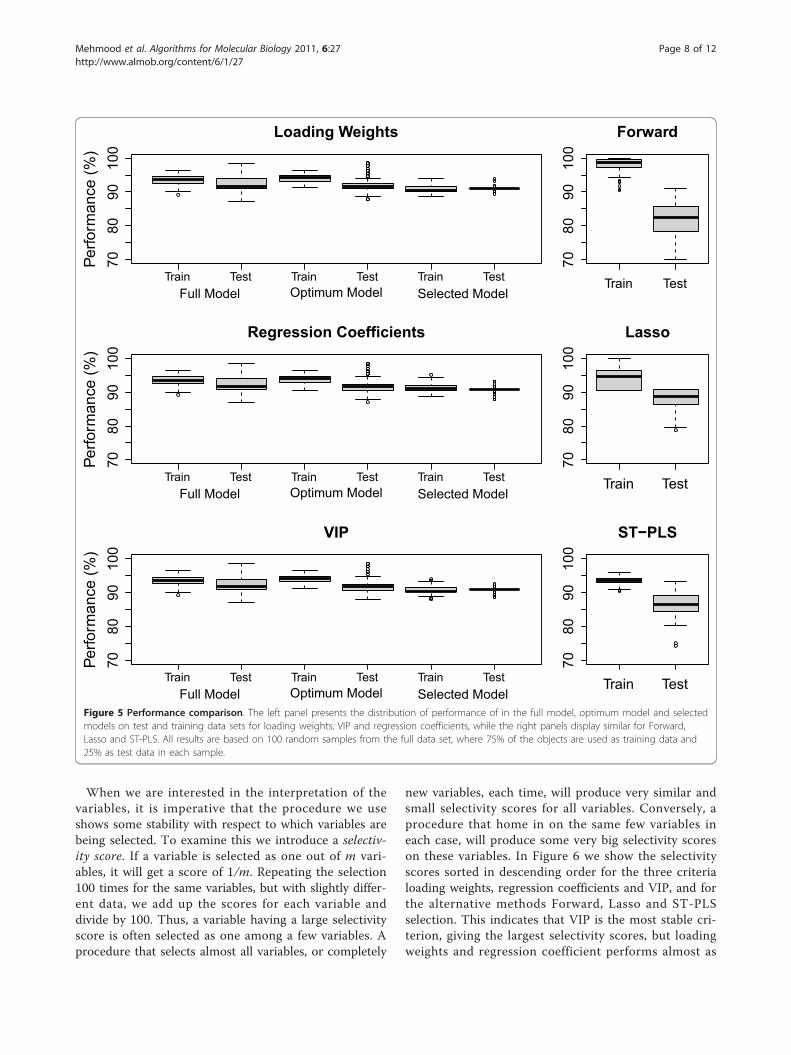
data sets are examined in Figure 5. In the left panels weshow the results for our procedure using the criterialoading weights, regression coefficient and VIP duringselection. In general all three criteria behave equally well.As expected, the best performance is found in the train-ing data for the ‘optimum’ model. Also, performance is

consistently worse in the test data compared to the train-ing data for all cases, but this pattern is most clearly pre-sent for the ‘optimum’ model. This may be seen as anindication of over-fitting. A huge variation in test dataperformance can be observed for the full model, andslightly smaller for the ‘optimum’ model. Our selectedmodels give somewhat worse overall training perfor-mance, but evaluated on the test sets they come out atthe same level as the ‘optimum’ model, and with a muchsmaller variance.In the right hand panels, performance is shown for the

three alternative methods. Our algorithm comes outwith at least as good performance on the test sets asany of the three alternative methods. Particularly notablyis the larger variation in test performance for the alter-native methods compared to the selected models in theleft panels. A formal testing by the Mann-Whitney test[63] indicates that our suggested procedure with VIPoutperforms Lasso (p < 0.001), Forward (p < 0.001) andST-PLS (p < 0.001) on the data sets used in this study.The same was also true if we used loading weights orregression coefficient as ranking criteria.

0 20 40 60 80

Loading Weights

Relative Size (%)

Optimum Model

Selected Model

0 20 40 60 80

Regression Coefficients

Relative Size (%)0 20 40 60 80

VIP

Relative Size (%)

0 20 40 60 80

Forward

Relative Size (%)

Fitted model

0 20 40 60 80

Lasso

Relative Size (%)0 20 40 60 80

ST−PLS

Relative Size (%)Figure 4 The distribution of selected variables. The distribution of the number of variables selected by the optimum model and selectedmodel for loading weights, VIP and regression coefficients is presented in upper panels, while lower panels display similar for Forward, Lassoand ST-PLS. The horizontal axes are the number of retained variables as percentage of the full model (with 4160 variables). All results are basedon 100 random samples from the full data set, where 75% of the objects are used as training data and 25% as test data in each sample.


of 12

When we are interested in the interpretation of thevariables, it is imperative that the procedure we useshows some stability with respect to which variables arebeing selected. To examine this we introduce a selectiv-ity score. If a variable is selected as one out of m vari-ables, it will get a score of 1/m. Repeating the selection100 times for the same variables, but with slightly differ-ent data, we add up the scores for each variable anddivide by 100. Thus, a variable having a large selectivityscore is often selected as one among a few variables. Aprocedure that selects almost all variables, or completely

new variables, each time, will produce very similar andsmall selectivity scores for all variables. Conversely, aprocedure that home in on the same few variables ineach case, will produce some very big selectivity scoreson these variables. In Figure 6 we show the selectivityscores sorted in descending order for the three criterialoading weights, regression coefficients and VIP, and forthe alternative methods Forward, Lasso and ST-PLSselection. This indicates that VIP is the most stable cri-terion, giving the largest selectivity scores, but loadingweights and regression coefficient performs almost as

7080

9010

0Loading Weights

Perfo

rman

ce (%

)

Train Test Train Test Train TestFull Model Optimum Model Selected Model

7080

9010

0


Perfo

rman

ce (%

)


7080

9010

0

VIP

Perfo

rman

ce (%

)


7080

9010

0

Forward

Train Test

7080

9010

0

Lasso

Train Test

7080

9010

0

ST−PLS

Train Test

Figure 5 Performance comparison. The left panel presents the distribution of performance of in the full model, optimum model and selectedmodels on test and training data sets for loading weights, VIP and regression coefficients, while the right panels display similar for Forward,Lasso and ST-PLS. All results are based on 100 random samples from the full data set, where 75% of the objects are used as training data and25% as test data in each sample.


of 12

good. The Lasso method is as stable as our proposedmethod using the VIP criterion, while Forward and ST-PLS seems worse as they spread the selectivity scoreover many more variables. From the definition of VIPwe know that the importance of the variables is down-weighted as number of CPPLS components increases.This probably reduces the noise influence and thus pro-vides more stable and consistent selection, also observedby [22].

95% of our selected model uses 1 component whilethe rest uses 2 components. It is clear from the defini-tion of Loading weights, VIP and regression coefficientsthat the sorted index of variables based on these mea-sures will be the same for 1 component. This could bethe reason for the rather similar behavior of loadingweights, VIP and regression coefficient in above analysis.In order to get a rough idea of the ‘null-distribution’

of this selectivity score, we ran the selection on data

0 100 200 300 400 5000.00

00.

025

Loading Weights

Sorted index of variables

Sel

ectiv

ity s

core

0 100 200 300 400 5000.00

00.

025

Forward


Sel

ectiv

ity s

core

0 100 200 300 400 5000.00

00.

025

VIP


Sel

ectiv

ity s

core

0 100 200 300 400 5000.00

00.

025

Lasso


Sel

ectiv

ity s

core

0 100 200 300 400 5000.00

00.

025



Sel

ectiv

ity s

core

0 100 200 300 400 5000.00

00.

025

ST−PLS


Sel

ectiv

ity s

core

Figure 6 Selectivity score. The selectivity score is sorted in descending order for each criterion loading weights, regression coefficientssignificance and VIP in the left panels, while right panels display similar for Forward, Lasso and ST-PLS. Only the first 500 values (out of 4160) areshown.


of 12

where the response y was permuted at random. Fromthis the upper 0.1% percentile of the null-distribution isdetermined, which is approximately corresponds to theselectivity score above 0.01. For each phylum and vari-ables giving a selectivity score above this percentile arelisted in Table 1. The selected variables will also havepositive or negative impact depending on the sign of theregression coefficients as indicated in the table. A di-codon with a positive/negative regression coefficient isinformative because it occurs more/less frequently inthis phylum than in the entire population. It appearsthat, the larger phyla are in general more difficult toclassify, simply because there are more diversity insidethe group. On the other hand, the results obtained forthe larger phyla are more relevant. Because a larger setof genomes usually means less sampling bias, i.e. thedata set represents the phylum better. Interestingly, allof the selected variables are di-codons (no singlecodons), providing additional support for that the inter-action of codons are highly important for explainingvariations in phyla [49,52,64]. It should be noted thatthe performance listed for each phylum in Table 1 is anoptimistic estimate of the real performance we mustexpect on a new data set, since it is based on variablesselected by maximizing performance over all data in the

present data set. However, for comparisons betweenphyla they are still relevant.

4 ConclusionWe have suggested a regularized backward eliminationalgorithm for variable selection using Partial LeastSquares, where the focus is to obtain a hard, and at thesame time stable, selection of variables. In our proposedprocedure, we compared three PLS-based selection cri-teria, and all produced good results with respect to sizeof selected model, model performance and selection sta-bility, with a slight overall improvement for the VIP cri-terion. We obtained a huge reduction in the number ofselected variables compared to using the models withoptimum performance based on training. The apparentloss in performance compared to the optimum basedmodels, as judged by the fit to the training set, is vir-tually disappearing when evaluated on a separate testset. Our selected model performs at least as good asthree alternative methods, Forward, Lasso and ST-PLS,on the present test data. This also indicates that the reg-ularized algorithm not only obtain models with superiorinterpretation potential, but also an improved stabilitywith respect to classification of new samples. A methodlike this could have many potential uses in genomics,

Table 1 Selectivity score based selected codons

Phylum Gen. Perf. Positive and Negative impact

Actinobacteria 42 90.6 TCCGTA, TACGGA, GTGAAG, CTTCAC, TGTACA, TCCGTT, AGAAGG, CCTTCT, GAGGCT, GGAACA,TCCACC, TGTTCC, TTCCGT, CTTAAG, GGGATC, GATCCC, CCTTAA, TTAAGG AACGGA, GGTGGA,GTCGAC,

Bacteroides 16 96.3 TATATA, TCTATA, CTATAT, TATAGA, ATATAG, TATAGT, TTATAG, CTTATA, CTATAA, ACTATA,TATATC, GATATA, CTATAG, TATACT TATAAG, ATATAT,

C renarchaeota 16 96.5 AACGCT, AGCGTT, ACGAGT, ACTCGT, ACGACT, TTAGGG, TCGTGT, ACACGA, CCCTAA, TAGCGT,TACGAG, ACGCTA, CGTGTT, AACACG, GGGCTA, CTACGA, TCGTAG, CGAGTA, TACTCG, GCGTTTAGTCGT, CTCGTA, TAGCCC,

Cyanobacteria 17 97.1 CAATTG, GTTCAA, TTGAAC, TAAGAC, GTCTTA, CTTAGT, TTAGTC, GGTCAA, GACTAA, ACTAAG,CTTGAT, AAGTCA, ATCAAG, TGGTTC, GAACCA, AGTCAA, GACCAA, TTGGTC, TTGATC, GACTTG,TCTTAG, CAAGTC TTGACC, TGACTT, TTGACT, GATCAA,

Euryarchaeota 31 93.3 ACACCG, CGGTGT, TCGGGT, GGTGTC, TCGGTG, CACCGA, ACCCGA, CCGCGG, GGTGTG, TCACCG,TATCGT, TACGCT, TTCTGC GACACC, CACACC,

Firmicutes 89 80.3 TCGGTA, TACCGA, ACAGGA, TCCTGT

Alphaproteobacteria 70 85.9 TCGCGA, AAGATC, GATCTT, TTCGCG, AAATTT, CGCGAA

Betaproteobacteria 42 90.8 GGAACA, TGTTCC, TAGTCG, CGACTA, GCTAGC, AAGCTC, GAGCTT, TACGAG, CTCGTA, CTTGCA,GATCTT, TGCAAG, AAGATC, AGGCTT, AAGCCT, CTCGAG

Gammaproteobacteria 92 81.2 CTCAGT, ACTGAG, GACTCA, TGAGTC, ACTCAG, ACTCTG, CAGAGT, CTCAGA, TCTGAG, CTGTCT,CCAGAG, CTCTGG, TCACCT, TGACTC, CTCTGT, AGGTGA, GAGTCA, TCACTC, GAGTGA CTGAGT,AGACAG, ACAGAG,

Deltaproteobacteria 18 96.0 GACATT, TCATGT, ACATGA, AATGTC, AACATC, ATGTTG, CAACAT, CATTGT, ACAATG, ACATTG,ACAACA, TGTTGT, AACAAC, GTTGTT, CATTTC, GTTCCA, TGGAAC, CAACAA, TTGTTG, GAAACA,GGAACA, TGTTCC, AATGAC, GTCATT GATGTT, CAATGT, GAAATG, TGTTTC,

Epsilonproteobacteria 12 96.9 TCCTGT, ACAGGA, GTATCC, TCAGGA, TCCTGA, TGCAGA, TCTGCA, TTCAGG, CCTGAA, ATATCC,GAACCT, AGGTTC, GGAGAT, ATCTCC, TTGCAG, GGATAC, GGATAT, CTGCAA, TCCCTG, CAGGGA,ACTGCA, TGCAGT, TTCCTG, TACAGG

Results obtained for each phylum by using the VIP criterion. Gen. is the number of genomes for that phylum in the data set, Perf. is the average test-setperformance i.e. percentage of correctly classified samples, when classifying the corresponding phylum. This is synonymous to the true positive rate. Positiveimpact variables are variables with selectivity score above 0.01 and with positive regression coefficients while Negative impact variables are similar with negativeregression coefficients.


of 12

but more comprehensive testing is needed to establishthe full potential. This proof of principle study shouldbe extended by multi-class classification problems aswell as regression problems before a final conclusioncan be drawn. From the data set used here we find asmallish number of di-codons associated with variousbacterial phyla, which is motivated by the recognition ofbacterial phyla in metagenomics studies. However, anytype of genome-wide association study may potentiallybenefit from the use of a multivariate selection methodlike this.

AcknowledgementsTahir Mehmoods scholarship has been fully financed by the HigherEducation Commission of Pakistan, Jonas Warringer was supported by grantsfrom the Royal Swedish Academy of Sciences and Carl Trygger Foundation.

Author details1Biostatistics, Department of Chemistry, Biotechnology and Food Sciences,Norwegian University of Life Sciences, Norway. 2Centre of IntegrativeGenetics (CIGENE), Animal and Aquacultural Sciences, Norwegian Universityof Life Sciences, Norway. 3Department of Cell- and Molecular Biology,University of Gothenburg, Sweden.

Authors’ contributionsTM and LS initiated the project and the ideas. All authors have beeninvolved in the later development of the approach and the final algorithm.TM has done the programming, with some assistance from SS and LS. TMand LS has drafted the manuscript, with inputs from all other authors. Allauthors have read and approved the final manuscript.

Competing interestsThe authors declare that they have no competing interests.

Received: 28 September 2011 Accepted: 5 December 2011Published: 5 December 2011

References1. Bachvarov B, Kirilov K, Ivanov I: Codon usage in prokaryotes. Biotechnology

and Biotechnological Equipment 2008, 22(2):669.2. Binnewies T, Motro Y, Hallin P, Lund O, Dunn D, La T, Hampson D,

Bellgard M, Wassenaar T, Ussery D: Ten years of bacterial genomesequencing: comparative-genomics-based discoveries. Functional &integrative genomics 2006, 6(3):165-185.

3. Shendure J, Porreca G, Reppas N, Lin X, McCutcheon J, Rosenbaum A,Wang M, Zhang K, Mitra R, Church G: Accurate multiplex polonysequencing of an evolved bacterial genome. Science 2005,309(5741):1728.

4. Hastie T, Tibshirani R, Friedman J: The Elements of Statistical Learning.2008.

5. Fernández Pierna J, Abbas O, Baeten V, Dardenne P: A Backward VariableSelection method for PLS regression (BVSPLS). Analytica chimica acta2009, 642(1-2):89-93.

6. Riaz K, Elmerich C, Moreira D, Raffoux A, Dessaux Y, Faure D: Ametagenomic analysis of soil bacteria extends the diversity ofquorum-quenching lactonases. Environmental Microbiology 2008,10(3):560-570.

7. Suzuki H, Brown C, Forney L, Top E: Comparison of correspondenceanalysis methods for synonymous codon usage in bacteria. DNA Research2008, 15(6):357.

8. Martens H, Næs T: Multivariate Calibration Wiley; 1989.9. Keleş S, Chun H: Comments on: Augmenting the bootstrap to analyze

high dimensional genomic data. TEST 2008, 17:36-39.10. Höskuldsson A: Variable and subset selection in PLS regression.

Chemometrics and Intelligent Laboratory Systems 2001, 55(1-2):23-38.

11. Boulesteix A, Strimmer K: Partial least squares: a versatile tool for theanalysis of high-dimensional genomic data. Briefings in Bioinformatics2007, 8:32.

12. John G, Kohavi R, Pfleger K: Irrelevant features and the subset selectionproblem. In Proceedings of the eleventh international conference on machinelearning. Volume 129. Citeseer; 1994:121-129.

13. Jouan-Rimbaud D, Walczak B, Massart D, Last I, Prebble K: Comparison ofmultivariate methods based on latent vectors and methods based onwavelength selection for the analysis of near-infrared spectroscopicdata. Analytica Chimica Acta 1995, 304(3):285-295.

14. Alsberg B, Kell D, Goodacre R: Variable selection in discriminant partialleast-squares analysis. Anal Chem 1998, 70(19):4126-4133.

15. Trygg J, Wold S: Orthogonal projections to latent structures (O-PLS).Journal of Chemometrics 2002, 16(3):119-128.

16. Boulesteix A: PLS dimension reduction for classification with microarraydata. Statistical Applications in Genetics and Molecular Biology 2004, 3:1075.

17. Sæbø S, Almøy T, Aarøe J, Aastveit AH: ST-PLS: a multi-dimensionalnearest shrunken centroid type classifier via PLS. Jornal of Chemometrics2007, 20:54-62.

18. Centner V, Massart D, de Noord O, de Jong S, Vandeginste B, Sterna C:Elimination of uninformative variables for multivariate calibration. AnalChem 1996, 68(21):3851-3858.

19. Osborne S, Künnemeyer R, Jordan R: Method of wavelength selection forpartial least squares. The Analyst 1997, 122(12):1531-1537.

20. Cai W, Li Y, Shao X: A variable selection method based on uninformativevariable elimination for multivariate calibration of near-infrared spectra.Chemometrics and Intelligent Laboratory Systems 2008, 90(2):188-194.

21. Eriksson L, Johansson E, Kettaneh-Wold N, Wold S: Multi-and megavariatedata analysis Umetrics Umeå; 2001.

22. Gosselin R, Rodrigue D, Duchesne C: A Bootstrap-VIP approach forselecting wavelength intervals in spectral imaging applications.Chemometrics and Intelligent Laboratory Systems 2010, 100:12-21.

23. Xiaobo Z, Jiewen Z, Povey M, Holmes M, Hanpin M: Variables selectionmethods in near-infrared spectroscopy. Analytica chimica acta 2010,667(1-2):14-32.

24. Frank I: Intermediate least squares regression method. Chemometrics andIntelligent Laboratory Systems 1987, 1(3):233-242.

25. Kettaneh-Wold N, MacGregor J, Dayal B, Wold S: Multivariate design ofprocess experiments (M-DOPE). Chemometrics and Intelligent LaboratorySystems 1994, 23:39-50.

26. Lindgren F, Geladi P, Rännar S, Wold S: Interactive variable selection (IVS)for PLS. Part 1: Theory and algorithms. Journal of Chemometrics 1994,8(5):349-363.

27. Liu F, He Y, Wang L: Determination of effective wavelengths fordiscrimination of fruit vinegars using near infrared spectroscopy andmultivariate analysis. Analytica chimica acta 2008, 615:10-17.

28. Frenich A, Jouan-Rimbaud D, Massart D, Kuttatharmmakul S, Galera M,Vidal J: Wavelength selection method for multicomponentspectrophotometric determinations using partial least squares. TheAnalyst 1995, 120(12):2787-2792.

29. Spiegelman C, McShane M, Goetz M, Motamedi M, Yue Q, Cot’e G:Theoretical justification of wavelength selection in PLS calibration:development of a new algorithm. Anal Chem 1998, 70:35-44.

30. Martens H, Martens M: Multivariate Analysis of Quality-An Introduction Wiley;2001.

31. Lazraq A, Cleroux R, Gauchi J: Selecting both latent and explanatoryvariables in the PLS1 regression model. Chemometrics and IntelligentLaboratory Systems 2003, 66(2):117-126.

32. Huang X, Pan W, Park S, Han X, Miller L, Hall J: Modeling the relationshipbetween LVAD support time and gene expression changes in thehuman heart by penalized partial least squares. Bioinformatics 2004, 4991.

33. Ferreira A, Alves T, Menezes J: Monitoring complex media fermentationswith near-infrared spectroscopy: Comparison of different variableselection methods. Biotechnology and bioengineering 2005, 91(4):474-481.

34. Xu H, Liu Z, Cai W, Shao X: A wavelength selection method based onrandomization test for near-infrared spectral analysis. Chemometrics andIntelligent Laboratory Systems 2009, 97(2):189-193.

35. Olah M, Bologa C, Oprea T: An automated PLS search for biologicallyrelevant QSAR descriptors. Journal of computer-aided molecular design2004, 18(7):437-449.


of 12

http://www.ncbi.nlm.nih.gov/pubmed/22148115?dopt=Abstract




























36. Chong G, Jun CH: Performance of some variable selection methodswhen multicollinearity is present. Chemo-metrics and Intelligent LaboratorySystems 2005, 78:103-112.

37. ElMasry G, Wang N, Vigneault C, Qiao J, ElSayed A: Early detection of applebruises on different background colors using hyperspectral imaging.LWT-Food Science and Technology 2008, 41(2):337-345.

38. Aha D, Bankert R: A comparative evaluation of sequential featureselection algorithms. Springer-Verlag, New York; 1996.

39. Ye S, Wang D, Min S: Successive projections algorithm combined withuninformative variable elimination for spectral variable selection.Chemometrics and Intelligent Laboratory Systems 2008, 91(2):194-199.

40. Ramadan Z, Song X, Hopke P, Johnson M, Scow K: Variable selection inclassification of environmental soil samples for partial least square andneural network models. Analytica chimica acta 2001, 446(1-2):231-242.

41. Indahl U, Liland K, Næs T: Canonical partial least squares: A unified PLSapproach to classification and regression problems. Journal ofChemometrics 2009, 23(9):495-504.

42. Ripley B: Pattern recognition and neural networks Cambridge Univ Pr; 2008.43. Naes T, Helland I: Relevant components in regression. Scandinavian

journal of statistics 1993, 20(3):239-250.44. Agresti A: In Categorical data analysis. Volume 359. John Wiley and Sons;

2002.45. Tibshirani R: Regression shrinkage and selection via the lasso. Journal of

the Royal Statistical Society. Series B (Methodological) 1996, 267-288.46. Haury A, Gestraud P, Vert J: The influence of feature selection methods

on accuracy, stability and inter-pretability of molecular signatures. Arxivpreprint arXiv:1101.5008 2011.

47. Lai D, Yang X, Wu G, Liu Y, Nardini C: Inference of gene networksapplication to Bifidobacterium. Bioinformatics 2011, 27(2):232.

48. Mehmood T, Martens H, Saebo S, Warringer J, Snipen L: Mining forGenotype-Phenotype Relations in Saccha-romyces using Partial LeastSquares. BMC bioinformatics 2011, 12:318.

49. Hanes A, Raymer M, Doom T, Krane D: A Comparision of Codon UsageTrends in Prokaryotes. 2009 Ohio Collaborative Conference on BioinformaticsIEEE; 2009, 83-86.

50. Chen R, Yan H, Zhao K, Martinac B, Liu G: Comprehensive analysis ofprokaryotic mechanosensation genes: Their characteristics in codonusage. Mitochondrial DNA 2007, 18(4):269-278.

51. Zavala A, Naya H, Romero H, Musto H: Trends in codon and amino acidusage in Thermotoga maritima. Journal of molecular evolution 2002,54(5):563-568.

52. Nguyen M, Ma J, Fogel G, Rajapakse J: Di-codon usage for geneclassification. Pattern Recognition in Bioinformatics 2009, 211-221.

53. Sharp P, Li W: The codon adaptation index-a measure of directionalsynonymous codon usage bias, and its potential applications. Nucleicacids research 1987, 15(3):1281.

54. Ikemura T: Correlation between the abundance of Escherichia colitransfer RNAs and the occurrence of the respective codons in its proteingenes: A proposal for a synonymous codon choice that is optimal forthe E. coli translational system* 1. Journal of molecular biology 1981,151(3):389-409.

55. Wright F: The effective number of codons’ used in a gene. Gene 1990,87:23-29.

56. Petrosino J, Highlander S, Luna R, Gibbs R, Versalovic J: Metagenomicpyrosequencing and microbial identification. Clinical chemistry 2009,55(5):856.

57. Riesenfeld C, Schloss P, Handelsman J: Metagenomics: genomic analysis ofmicrobial communities. Annu Rev Genet 2004, 38:525-552.

58. Ellis J, Griffin H, Morrison D, Johnson A: Analysis of dinucleotide frequencyand codon usage in the phylum Apicomplexa. Gene 1993, 126(2):163-170.

59. Lightfield J, Fram N, Ely B, Otto M: Across Bacterial Phyla, Distantly-Related Genomes with Similar Genomic GC Content Have SimilarPatterns of Amino Acid Usage. PloS one 2011, 6(3):e17677.

60. Kotamarti M, Raiford D, Dunham M: A Data Mining Approach toPredicting Phylum using Genome-Wide Sequence Data..

61. Hyatt D, Chen GL, Locascio PF, Land ML, Larimer FW, Hauser LJ: Prodigal:prokaryotic gene recognition and translation initiation site identification.BMC Bioinformatics 2010, 11:119.

62. Anderssen E, Dyrstad K, Westad F, Martens H: Reducing over-optimism invariable selection by cross-model validation. Chemometrics and intelligentlaboratory systems 2006, 84(1-2):69-74.

63. Wolfe D, Hollander M: Nonparametric statistical methods. Nonparametricstatistical methods 1973.

64. Newman J, Ghaemmaghami S, Ihmels J, Breslow D, Noble M, DeRisi J,Weissman J: Single-cell proteomic analysis of S. cerevisiae reveals thearchitecture of biological noise. Nature 2006, 441(7095):840-846.

doi:10.1186/1748-7188-6-27Cite this article as: Mehmood et al.: A Partial Least Squares basedalgorithm for parsimonious variable selection. Algorithms for MolecularBiology 2011 6:27.

Submit your next manuscript to BioMed Centraland take full advantage of:

• Convenient online submission

• Thorough peer review

• No space constraints or color figure charges

• Immediate publication on acceptance

• Inclusion in PubMed, CAS, Scopus and Google Scholar

• Research which is freely available for redistribution

Submit your manuscript at www.biomedcentral.com/submit


of 12




























A Partial Least Squares based algorithm for parsimonious variable

Documents

Transcript of A Partial Least Squares based algorithm for parsimonious variable