University of Groningen

Partial least squares path modeling using ordinal categorical indicatorsSchuberth, Florian; Henseler, Jorg; Dijkstra, Theo K.

Published in:Quality & Quantity

DOI:10.1007/s11135-016-0401-7

IMPORTANT NOTE: You are advised to consult the publisher's version (publisher's PDF) if you wish to cite fromit. Please check the document version below.

Document VersionPublisher's PDF, also known as Version of record

Publication date:2018

Link to publication in University of Groningen/UMCG research database

Citation for published version (APA):Schuberth, F., Henseler, J., & Dijkstra, T. K. (2018). Partial least squares path modeling using ordinalcategorical indicators. Quality & Quantity, 52(1), 9-35. https://doi.org/10.1007/s11135-016-0401-7

CopyrightOther than for strictly personal use, it is not permitted to download or to forward/distribute the text or part of it without the consent of theauthor(s) and/or copyright holder(s), unless the work is under an open content license (like Creative Commons).

Take-down policyIf you believe that this document breaches copyright please contact us providing details, and we will remove access to the work immediatelyand investigate your claim.

Downloaded from the University of Groningen/UMCG research database (Pure): http://www.rug.nl/research/portal. For technical reasons thenumber of authors shown on this cover page is limited to 10 maximum.

Download date: 20-03-2020

Partial least squares path modeling using ordinalcategorical indicators

Florian Schuberth1• Jorg Henseler2

• Theo K. Dijkstra3

� The Author(s) 2016. This article is published with open access at Springerlink.com

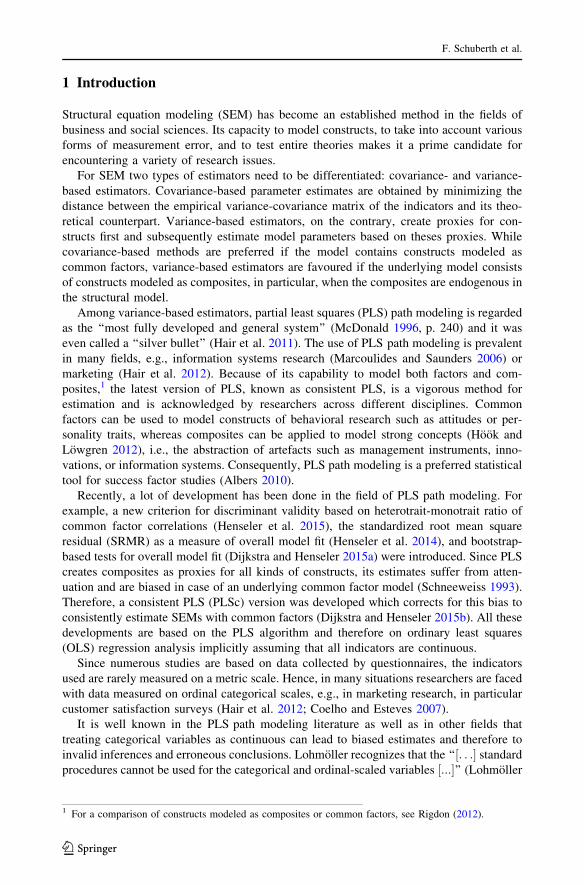
Abstract This article introduces a new consistent variance-based estimator called ordinal

consistent partial least squares (OrdPLSc). OrdPLSc completes the family of variance-

based estimators consisting of PLS, PLSc, and OrdPLS and permits to estimate structural

equation models of composites and common factors if some or all indicators are measured

on an ordinal categorical scale. A Monte Carlo simulation (N ¼ 500) with different

population models shows that OrdPLSc provides almost unbiased estimates. If all con-

structs are modeled as common factors, OrdPLSc yields estimates close to those of its

covariance-based counterpart, WLSMV, but is less efficient. If some constructs are

modeled as composites, OrdPLSc is virtually without competition.

Keywords Structural equation models � Consistent partial least squares � Ordinalcategorical indicators � Common factors � Composites � Polychoric correlation

Electronic supplementary material The online version of this article (doi:10.1007/s11135-016-0401-7)contains supplementary material, which is available to authorized users.

& Jorg Henselerj.henseler@utwente.nl

Florian Schuberthflorian.schuberth@uni-wuerzburg.de

Theo K. Dijkstrat.k.dijkstra@rug.nl

1 Faculty of Business Management and Economics, University of Wurzburg, Sanderring 2,97070 Wurzburg, Germany

2 Faculty of Engineering Technology, University of Twente, P.O. Box 217, 7500 AE Enschede,The Netherlands

3 Faculty of Economics and Business, University of Groningen, Nettelbosje 2, P.O. Box 800,9747 AE Groningen, The Netherlands

123

Qual QuantDOI 10.1007/s11135-016-0401-7

1 Introduction

Structural equation modeling (SEM) has become an established method in the fields of

business and social sciences. Its capacity to model constructs, to take into account various

forms of measurement error, and to test entire theories makes it a prime candidate for

encountering a variety of research issues.

For SEM two types of estimators need to be differentiated: covariance- and variance-

based estimators. Covariance-based parameter estimates are obtained by minimizing the

distance between the empirical variance-covariance matrix of the indicators and its theo-

retical counterpart. Variance-based estimators, on the contrary, create proxies for con-

structs first and subsequently estimate model parameters based on theses proxies. While

covariance-based methods are preferred if the model contains constructs modeled as

common factors, variance-based estimators are favoured if the underlying model consists

of constructs modeled as composites, in particular, when the composites are endogenous in

the structural model.

Among variance-based estimators, partial least squares (PLS) path modeling is regarded

as the ‘‘most fully developed and general system’’ (McDonald 1996, p. 240) and it was

even called a ‘‘silver bullet’’ (Hair et al. 2011). The use of PLS path modeling is prevalent

in many fields, e.g., information systems research (Marcoulides and Saunders 2006) or

marketing (Hair et al. 2012). Because of its capability to model both factors and com-

posites,1 the latest version of PLS, known as consistent PLS, is a vigorous method for

estimation and is acknowledged by researchers across different disciplines. Common

factors can be used to model constructs of behavioral research such as attitudes or per-

sonality traits, whereas composites can be applied to model strong concepts (Hook and

Lowgren 2012), i.e., the abstraction of artefacts such as management instruments, inno-

vations, or information systems. Consequently, PLS path modeling is a preferred statistical

tool for success factor studies (Albers 2010).

Recently, a lot of development has been done in the field of PLS path modeling. For

example, a new criterion for discriminant validity based on heterotrait-monotrait ratio of

common factor correlations (Henseler et al. 2015), the standardized root mean square

residual (SRMR) as a measure of overall model fit (Henseler et al. 2014), and bootstrap-

based tests for overall model fit (Dijkstra and Henseler 2015a) were introduced. Since PLS

creates composites as proxies for all kinds of constructs, its estimates suffer from atten-

uation and are biased in case of an underlying common factor model (Schneeweiss 1993).

Therefore, a consistent PLS (PLSc) version was developed which corrects for this bias to

consistently estimate SEMs with common factors (Dijkstra and Henseler 2015b). All these

developments are based on the PLS algorithm and therefore on ordinary least squares

(OLS) regression analysis implicitly assuming that all indicators are continuous.

Since numerous studies are based on data collected by questionnaires, the indicators

used are rarely measured on a metric scale. Hence, in many situations researchers are faced

with data measured on ordinal categorical scales, e.g., in marketing research, in particular

customer satisfaction surveys (Hair et al. 2012; Coelho and Esteves 2007).

It is well known in the PLS path modeling literature as well as in other fields that

treating categorical variables as continuous can lead to biased estimates and therefore to

invalid inferences and erroneous conclusions. Lohmoller recognizes that the ‘‘ . . .½ � standardprocedures cannot be used for the categorical and ordinal-scaled variables :::½ �’’ (Lohmoller

1 For a comparison of constructs modeled as composites or common factors, see Rigdon (2012).

F. Schuberth et al.

123

2013, Chap. 4). Also Hair et al. (2012) mention that PLS is often used with categorical

indicators but that their use in a procedure like PLS which uses OLS as estimator can be

problematic. Several approaches to address this issue in the context of PLS are provided by

the literature, e.g., ordinal PLS (OrdPLS) an innovative approach to deal with ordinal

categorical indicators in a psychometric way (Cantaluppi 2012; Cantaluppi and Boari

2016). As OrdPLS is based on the traditional PLS algorithm, its use is limited to models

where all constructs are modeled as composites. However, researchers often deal with

models containing constructs modeled as common factors instead of composites (Ringle

et al. 2012; Hair et al. 2012). So, there is a real need for improving methods like OrdPLS

to be able to deal with common factors, composites and ordinal categorical indicators.

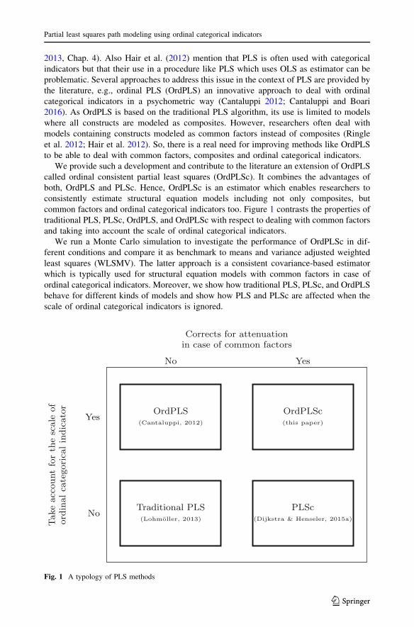
We provide such a development and contribute to the literature an extension of OrdPLS

called ordinal consistent partial least squares (OrdPLSc). It combines the advantages of

both, OrdPLS and PLSc. Hence, OrdPLSc is an estimator which enables researchers to

consistently estimate structural equation models including not only composites, but

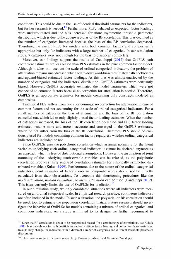
common factors and ordinal categorical indicators too. Figure 1 contrasts the properties of

traditional PLS, PLSc, OrdPLS, and OrdPLSc with respect to dealing with common factors

and taking into account the scale of ordinal categorical indicators.

We run a Monte Carlo simulation to investigate the performance of OrdPLSc in dif-

ferent conditions and compare it as benchmark to means and variance adjusted weighted

least squares (WLSMV). The latter approach is a consistent covariance-based estimator

which is typically used for structural equation models with common factors in case of

ordinal categorical indicators. Moreover, we show how traditional PLS, PLSc, and OrdPLS

behave for different kinds of models and show how PLS and PLSc are affected when the

scale of ordinal categorical indicators is ignored.

Traditional PLS)3102,rellomhoL(

PLSc(Dijkstra & Henseler, 2015a)

OrdPLS(Cantaluppi, 2012)

OrdPLSc(this paper)

Yes

No

No Yes

Corrects for attenuationin case of common factors

Tak

eac

coun

tforth

escaleof

ordina

lca

tego

rica

lindica

tor

Fig. 1 A typology of PLS methods

Partial least squares path modeling using ordinal categorical indicators

123

The remainder of the paper is organized as follows: The next section shows the

development from PLS to PLSc and provides a reformulation of these two procedures in

terms of indicators correlation matrices. In Sect. 3 we give a literature review of existing

approaches dealing with categorical indicators in the framework of PLS, in particular we

present the idea of the OrdPLS approach. In Sect. 4 we introduce ordinal consistent PLS

(OrdPLSc) to the literature. In the following Sect. 5, we present the design of our Monte

Carlo simulation, which is conducted to examine the performance of OrdPLSc and dif-

ferent other estimators under several conditions. We present these findings in Sect. 6. The

article closes with the discussion of the results in Sect. 7. An Appendix covers the figure of

the threshold parameter distribution.

2 The development from PLS path modeling to consistent PLS pathmodeling

PLS was developed by Wold (1975) for the analysis of high dimensional data in a low-

structure environment and has undergone various extensions and modifications. It is an

approach similar to generalized canonical correlation analysis (GCCA), and in addition

able to emulate several of Kettenring (1971)’s techniques for the canonical analysis of

several sets of variables (Tenenhaus et al. 2005).

In its most modern appearance known as consistent PLS (PLSc) (Dijkstra and Henseler

2015a, b), it can be understood as a well-developed SEM method. It is capable to estimate

recursive and non-recursive structural models with constructs modeled as composites and

common factors. Both obtain the outer weights and the final stand-ins for the constructs by

the classical PLS algorithm. While traditional PLS simply relies on OLS to estimate the

model parameters, its extended version, PLSc, uses two-stage least squares (2SLS) to

consistently estimate even non-recursive path models. Furthermore, PLSc is able to handle

both constructs modeled as composites and as common factors by using a post-correction

for attenuation for correlations between common factors, and common factors and

indicators.

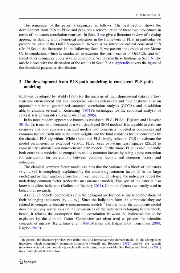
The classical common factor model assumes that the variance of a block of indicators

ðx1; . . .; xKÞ is completely explained by the underlying common factor (n in the large

circle) and by their random errors ð�1; . . .; �KÞ, see Fig. 2a. Hence, the indicators reflect theunderlying common factor (reflective measurement model). This sort of indicator is also

known as effect indicators (Bollen and Bauldry 2011). Common factors are usually used in

behavioral research.

As Fig. 2b depicts, composites (n in the hexagon) are formed as linear combinations of

their belonging indicators ðx1; . . .; xKÞ. Since the indicators form the composite, they are

related to composite-formative measurement models.2 Furthermore, the composite model

does not put any restrictions on the covariances of the indicators belonging to one block,

hence, it relaxes the assumption that all covariation between the indicators has to be

explained by the common factor. Composites are often used as proxies for scientific

concepts of interest (Ketterlinus et al. 1989; Maraun and Halpin 2008; Tenenhaus 2008;

Rigdon 2012).

2 In general, the literature provides two definitions of a formative measurement model: (i) the (composite)indicators which completely determine composite (Fornell and Bookstein 1982), and (ii) the (causal)indicators which do not completely explain the underlying latent variable. See Bollen and Bauldry (2011)for a more detailed description.

F. Schuberth et al.

123

For the derivation of OrdPLS(c) it is crucial to describe the well-known PLS algorithm

(Wold 1975) and its extension to PLSc in terms of indicator covariances or correlations,

respectively. Since in PLS no distinction between exogenous and endogenous constructs is

made, we use the following notation: g is a ðJ � 1Þ vector containing all modeled con-

structs which are connected by the structural model, whether they are modeled as common

factors or as composites. The ðK � 1Þ vector x contains all indicators which measure the

common factors or build the composites, respectively.

2.1 Partial least squares

For a sample of size n, all observations of the K indicators are stacked in a data matrix X of

dimension ðn� KÞ. For simplicity, the Kj indicators belonging to one common factor or

one composite gj are grouped to form block j with j ¼ 1; . . .; J. Observations of block j are

stacked in the data matrix Xj of dimension ðn� KjÞ withPJ

j¼1 Kj ¼ K. Furthermore, we

assume that each indicator is standardized, as is customary in PLS, to have mean zero and

unit variance, such that the indicators’ sample covariance matrix S equals the sample

correlation matrix.

The PLS estimation procedure consists of three parts. In the first part, for each block j

initial arbitrary outer weights wð0Þj ðKj � 1Þ are chosen which satisfy the following con-

dition: wð0Þ0j Sjjw

ð0Þj ¼ 1 where the Kj � Kj matrix Sjj contains the sample correlations of the

indicators of block j. This condition holds for all outer weights in each iteration i and can

be achieved by using the scaling factor ðwðiÞ0j Sjjw

ðiÞj Þ�

12 for the outer weights w

ðiÞj in each

iteration.

In the second part, the iterative PLS algorithm starts with step one, the outer approx-

imation of gj:

gðiÞj ¼ Xjw

ðiÞj with w

ðiÞ0j Sjjw

ðiÞj ¼ 1; ð1Þ

where gðiÞj is a column vector of length n. Since outer weights are scaled, all outer proxies

also have mean zero and unit variance.

xk· · ·x1 · · · xK

ξ

ε1 εKεk· · · · · ·

xk· · ·x1 · · · xK

ξ

(a) Common factor model (b) Composite model

Fig. 2 Common factor versus composite

Partial least squares path modeling using ordinal categorical indicators

123

In the second step, the inner proxy of gj is calculated as a linear combination of inner

weights and outer proxies of gj0 :

~gðiÞj ¼

XJ

j0¼1

eðiÞjj0 g

ðiÞj0 ; ð2Þ

where ~gðiÞj is again a column vector of length n. The inner weight ejj0 defines how the inner

proxy ~gj is built. Three different schemes for the calculation of ejj0 are commonly used:

centroid (Wold 1982), factorial (Lohmoller 2013), and path weighting. However, all

schemes yield essentially the same results (Noonan and Wold 1982), hence, we only

consider the centroid scheme.3 The inner weights are chosen according to the signs of the

correlations between the outer proxies

eðiÞjj0 ¼

signðwðiÞ0j Sjj0 w

ðiÞj0 Þ; for j 6¼ j0 and if construct j and j0 are adjacent

0; otherwise;

(

ð3Þ

where adjacent refers to the constructs j and j0 directly connected by the structural model.

All inner proxies ~gðiÞj are again scaled to have unit variance.

In the third and last step of the iterative part, new outer weights are calculated. This can

be done in three ways: mode A, mode B, and mode C. For mode A, estimated outer weights

of block j equal the estimated coefficients of a multivariate regression from the indicators

of block j on its related inner proxy. Due to standardization, the new estimated outer

weights wðiþ1Þj equal the correlations between the inner proxy and its related indicators:

wðiþ1Þj /

XJ

j0¼1

Sjj0 wðiÞj0 e

ðiÞjj0 with w

ðiþ1Þ0j Sjjw

ðiþ1Þj ¼ 1: ð4Þ

In contrast, for mode B, the new outer weights equal the estimated coefficients of a

regression from the inner proxy on its connected indicators:

wðiþ1Þj / S�1

jj

XJ

j0¼1

Sjj0 wðiÞj0 e

ðiÞjj0 with w

ðiþ1Þ0j Sjjw

ðiþ1Þj ¼ 1: ð5Þ

Mode C, also known as MIMIC mode, is a mixture of mode A and mode B and is not

considered here.4

As the traditional PLS algorithm has no single optimization criteria to be minimized, the

new outer weights wðiþ1Þj are checked for significant changes compared to the outer weights

from the previous iteration step wðiÞj . If there is a significant change in the weights, the

algorithm starts again at step one by building new outer proxies with the new outer

weights, otherwise it stops.

In the last part, the obtained stable outer weights wj are used to build final composite

stand-ins for both common factors and composites: gj ¼ Xjwj. For constructs which are

modeled as common factors, the factor loadings are estimated by OLS in accordance with

3 For more details on the other schemes, see Tenenhaus et al. (2005).4 A consistent version of mode C, for any of its 2J - 2 implementations, can be obtained by using theproperties of mode A and mode B, see Dijkstra (1981, 1985, Chap. 2, par. 5.2), but since mode C isintermediate between the other modes, adding mode C does not really contribute to a further understanding.

F. Schuberth et al.

123

the measurement model. In contrast, for constructs which are modeled as composites the

final weights equal the stable weights from the last iteration. Finally, path coefficients are

estimated by OLS with respect to the structural model.

2.2 Consistent PLS

PLS is based on composites, which implies that estimates are biased if constructs are

modeled as common factors.5 In general, a composite model has larger absolute inter

composite correlations compared to the absolute inter common factor correlations of a

model with the same structure but where all constructs are modeled as common factors.

However, a transformation of the model-implied correlation matrix of a composite model

into the model-implied correlation matrix of a common factor model can be achieved by a

correction for attenuation (Cohen et al. 2013, Chap. 2.10). Consistent PLS (PLSc) uses this

correction to obtain consistent estimates for models containing common factors (Dijkstra

and Henseler 2015a, b). The correction requires that each common factor is measured by at

least two indicators and uses the proportionality between the population outer weights and

the population factor loadings, wj ¼ cjkj. The estimated correction factor for block j sat-

isfies the following condition

plimðcjÞ ¼ffiffiffiffiffiffiffiffiffiffiffiffiffik0jRjjkj

q; ð6Þ

where kj is a column vector of length Kj containing the population loadings of common

factor gj and Rjj is the Kj � Kj population correlation matrix of the indicators of block j.6

The correction factor cj can be obtained as

c2j ¼w0jðSjj � diagðSjjÞÞwj

w0jðwjw

0j � diagðwjw

0jÞÞwj

: ð7Þ

It is chosen such that the Euclidean distance between

Sjj � diagðSjjÞ and ðcjwjÞðcjwjÞ0 � diagððcjwjÞðcjw0jÞÞ ð8Þ

is minimized (Dijkstra and Henseler 2015a). Factor loadings of block j are consistently

estimated by

kj ¼ cjwj: ð9Þ

Moreover, PLSc is able to consistently estimate the path coefficients of recursive and non-

recursive models7 using OLS or 2SLS according to the structural model. Since all variables

are standardized, the estimated path coefficients are based on the correlations between the

columns of g ðn� JÞ. The correlation between the common factors j and j0 is consistentlyestimated by:

5 Both, common factors as well as composites are legit ways of construct modeling, see Rigdon (2012).6 The use of mode B for common factors is not considered here. For a consistent version of PLS using modeB see Dijkstra (1981, 2011).7 PLSc relaxes the assumptions of the basic design (Wold 1982) where non-recursive structural models arenot allowed.

Partial least squares path modeling using ordinal categorical indicators

123

ccorðgj; gj0 Þ ¼w0jSjj0 wj0

cjðw0jwjÞcj0 ðw0

j0 wj0 Þ: ð10Þ

Using the corrected correlation of Eq. (10) for the estimation of the structural model, one

obtains consistently estimated path coefficients between the common factors.8 For con-

structs which are modeled as composites no correction of the correlation is required

because, by construction, they are not affected by attenuation. In case construct j is

modeled as a common factor and construct j0 as a composite, the consistently estimated

correlation is obtained as

ccorðgj; gj0 Þ ¼w0jSjj0 wj0

cjðw0jwjÞ

: ð11Þ

3 The development from PLS to ordinal PLS

Since incorrectly handling ordinal categorical variables as continuous can lead to biased

inferences and therefore to erroneous conclusions, the literature provides several approa-

ches to deal with discrete indicators: dichotomize the ordinal categorical indicator, a

mixture of PLS and correspondence analysis (CA), Partial Maximum Likelihood PLS

(PML-PLS), and non-metric PLS (NM-PLS).

Common practice in PLS is to replace a categorical indicator by a dummy matrix which

is known as dichotomizing. Since each categorical indicator is replaced by s� 1 dummy

variables, where s is the number of observed categories, s� 1 outer weights are obtained

for the original variable. This contradicts the idea of treating an indicator as a whole.

Betzin and Henseler (2005) use correspondence analysis to quantify ex-ante categorical

indicators. As the quantified indicators are obtained, PLS is used to estimate the model

parameters. As a result, individual weights are obtained for each category of the categorical

indicator. Again, this has the drawback that no single outer weight for a categorical

indicator is calculated.

Partial Maximum Likelihood Partial Least Squares (PML-PLS) (Jakobowicz and Der-

quenne 2007) is a modified version of the original PLS algorithm. It is a combination of

PLS and generalized linear models designed to deal with indicators of any scale. For

categorical indicators, individual outer weights are computed for each category by

ANOVA. Based on those, one ’global’ weight per categorical indicator is calculated.

However, statistical properties like the proportionality of outer weights to factor loadings

are unknown for the global weights and further investigation is needed. Moreover, the

authors note that PML-PLS ‘‘is especially advantageous in the case of nominal or binary

variables’’ (Jakobowicz and Derquenne 2007) but we focus on ordinal categorical

indicators.

The last approach, non-metric partial least squares (NM-PLS) extends PLS by an

alternating least squares optimal scaling (ALSOS) algorithm to quantify qualitative indi-

cators and gain outer weights (Russolillo 2012). ALSOS is a procedure which quantifies

qualitative variables by preserving properties of the original measurement scales and

8 For more details, e.g., the consistent estimation of non-recursive models and the correction for nonlinearstructural equation models see Dijkstra (1983, 1981, 1985, 2010, 2011), Dijkstra and Schermelleh-Engel(2014).

F. Schuberth et al.

123

optimizes an objective optimization criteria by alternating least squares (Young 1981). In

the case of NM-PLS, the categorical indicator is quantified in a way that the correlation

between the inner proxy and the quantified categorical indicator is maximized. As a result

for each indicator one outer weight is obtained as in traditional PLS for continuous

indicators.

However, the evaluation of the presented approaches is based on empirical studies and,

to our knowledge, no simulation studies have been conducted to investigate their statistical

properties. For an extension to PLSc in order to deal with common factors, it is necessary

that the outer weights are proportional to the factor loadings. Moreover, the modified PLS

procedures are often applied to common factor models which represents a misspecified

model in the context of PLS. Hence, an assessment of their statistical properties is hardly

possible and we decided not to pursue any of the previously mentioned methods.

3.1 Ordinal PLS

A promising approach to deal with ordinal categorical indicators is ordinal PLS (OrdPLS9)

(Cantaluppi 2012). It is a modified procedure for handling ordinal categorical variables in a

classical psychometric way. In Sect. 2 we showed that all parameters can be obtained by

the use of the correlation matrix S. Traditional PLS uses the Bravais-Pearson (BP) cor-

relation matrix which requires all indicators to be continuous for consistency. The

observation of an ordinal categorical variable is a qualitative measure, yet it is often coded

as numeric and therefore mistakenly treated as quantitative by researchers. This routinely

happens in applications with binary and ordinal categorical indicators which results in

biased BP correlation estimates (Quiroga 1992; O’Brien and Homer 1987; Wylie 1976;

Carroll 1961). To fix this, OrdPLS uses a consistent correlation matrix as input for the

traditional PLS algorithm. An advantage of OrdPLS over the approaches previously

introduced is its transparent way of dealing with ordinal categorical variables. Moreover,

the original PLS algorithm remains untouched and it is just provided by a consistent

correlation matrix as input for the algorithm.

Since OrdPLS does not correct for attenuation, it shows the same drawbacks as PLS if

common factors are included in the model. Nevertheless, we consider OrdPLS as a

powerful extension of PLS when applied under appropriate circumstances, i.e., for models

with only composites. Furthermore, it is straightforward to extend by PLSc, to overcome

its drawback for common factor models, see Sect. 4. In the following subsection we

present Pearson’s considerations of ordinal categorical variables to provide a better

understanding of the polychoric and polyserial correlation.

3.2 Ordinal categorical variables according to Pearson

Pearson (1900, 1913) considers an ordinal categorical variable as a crude measure of an

underlying continuous random variable, while Yule (1900) assumes categorical variables

being inherently discrete. In this paper we follow Pearson’s idea: an observed ordinal

categorical indicator x is the result of a polytomized standard normally distributed random

variable x�:

9 OrdPLS was originally called OPLS (Cantaluppi 2012). An anonymous reviewer suggested to use adifferent name in order to avoid confounding with O-PLS (Trygg and Wold 2002). We came to anagreement with Cantaluppi to speak of OrdPLS in the future. We thank the anonymous reviewer forsuggesting such a disambiguation.

Partial least squares path modeling using ordinal categorical indicators

123

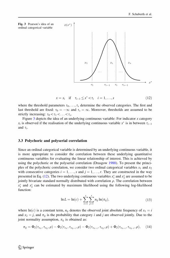
x ¼ xi if si�1 � x�\si i ¼ 1; . . .; s ð12Þ

where the threshold parameters s0; . . .; ss determine the observed categories. The first and

last threshold are fixed: s0 ¼ �1 and ss ¼ 1. Moreover, thresholds are assumed to be

strictly increasing: s0\s1\. . .\ss.Figure 3 depicts the idea of an underlying continuous variable: For indicator x category

xi is observed if the realisation of the underlying continuous variable x� is in between si�1

and si.

3.3 Polychoric and polyserial correlation

Since an ordinal categorical variable is determined by an underlying continuous variable, it

is more appropriate to consider the correlation between these underlying quantitative

continuous variables for evaluating the linear relationship of interest. This is achieved by

using the polychoric or the polyserial correlation (Drasgow 1988). To present the princi-

ples of the polychoric correlation, we consider two ordinal categorical variables x1 and x2with consecutive categories i ¼ 1; . . .; s and j ¼ 1; . . .; r. They are constructed in the way

presented in Eq. (12). The two underlying continuous variables x�1 and x�2 are assumed to be

jointly bivariate standard normally distributed with correlation q. The correlation between

x�1 and x�2 can be estimated by maximum likelihood using the following log-likelihood

function:

ln L ¼ lnðcÞ þXs

i¼1

Xr

j¼1

nij lnðpijÞ; ð13Þ

where lnðcÞ is a constant term, nij denotes the observed joint absolute frequency of x1 ¼ i

and x2 ¼ j, and pij is the probability that category i and j are observed jointly. Due to the

joint normality assumption, pij is obtained as:

pij ¼ U2ðsx1i ; sx2j ; qÞ � U2ðsx1i ; sx2j�1; qÞ � U2ðsx1i�1

; sx2j ; qÞ þ U2ðsx1i�1; sx2j�1

; qÞ; ð14Þ

τ1 τi−1 τi τs−1

. . . . . .

xix1 xs

x∗

φ(x∗)Fig. 3 Pearson’s idea of anordinal categorical variable

F. Schuberth et al.

123

where U2 is the cumulative distribution function of the bivariate standard normal distri-

bution. The parameters sx1i , sx2j , and q are chosen to maximize the function lnL. In order to

reduce computational burden, a two-step procedure can be used (Olsson 1979). In the first

step, threshold parameters are estimated separately as quantiles of cumulative marginal

frequencies, i.e., sx1i ¼ U�1ðpiÞ where pi equals the cumulative marginal relative frequency

up to category i and the function U�1 represents the quantile function of the standard

normal distribution (analogous for x2). Second, given the estimated threshold parameters,

Eq. (13) is maximized with respect to q. In case of a continuous and an ordinal categorical

variable, the correlation between the two continuous variables is obtained by the polyserial

correlation (Olsson et al. 1982). For more than two variables, a multivariate version is used

to estimate the correlations (Poon and Lee 1987). Moreover, a less computational intensive

two-step approach can be used for the multivariate version (Lee and Poon 1987). OrdPLS

as well as OrdPLSc makes use of the polychoric and polyserial correlation when ordinal

categorical indicators are part of the model.

4 Ordinal consistent partial least squares

We introduce a new approach which deals with common factors, composites, and ordinal

categorical indicators. It is called ordinal consistent partial least squares (OrdPLSc) and is

a combination of OrdPLS and PLSc. It uses the polychoric correlation, a consistent cor-

relation matrix in case of ordinal categorical indicators, as input for the PLS algorithm and

corrects for attenuation if common factors are included in the model. Since the use of the

polychoric correlation matrix does not affect the original PLS algorithm, the proportion-

ality property of the outer weights is maintained and the correction of attenuation can be

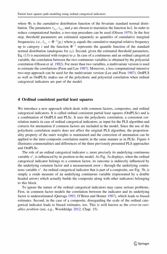
applied to the inter-composite correlation matrix in the same manner as in PLSc. Figure 4

illustrates commonalities and differences of the three previously presented PLS approaches

and OrdPLSc.

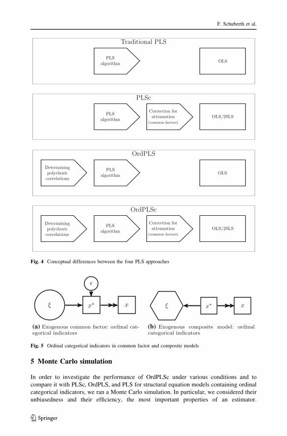
The role of an ordinal categorical indicator x, more precisely its underlying continuous

variable x�, is influenced by its position in the model. As Fig. 5a displays, when the ordinal

categorical indicator belongs to a common factor, its outcome is indirectly influenced by

the underlying common factor and a measurement error � through the underlying contin-

uous variable x�. An ordinal categorical indicator that is part of a composite, see Fig. 5b, is

simply a crude measure of an underlying continuous variable (represented by a double

headed arrow) which actually builds the composite along with other indicators belonging

to this block.

To ignore the nature of the ordinal categorical indicators may cause serious problems.

First, in common factor models the correlation between the indicator and its underlying

factor is underestimated (Quiroga 1992; O’Brien and Homer 1987), which leads to biased

estimates. Second, in the case of a composite, disregarding the scale of the ordinal cate-

gorical indicator leads to biased estimates, too. This is well known as the error-in-vari-

ables problem (see, e.g., Wooldridge 2012, Chap. 15).

Partial least squares path modeling using ordinal categorical indicators

123

5 Monte Carlo simulation

In order to investigate the performance of OrdPLSc under various conditions and to

compare it with PLSc, OrdPLS, and PLS for structural equation models containing ordinal

categorical indicators, we ran a Monte Carlo simulation. In particular, we considered their

unbiasedness and their efficiency, the most important properties of an estimator.

OLSPLS

algorithm

Traditional PLS

OLS/2SLSPLSalgorithm

Correction forattenuation

(common factors)

PLSc

OLSPLS

algorithm

Determiningpolychoriccorrelations

OrdPLS

Correction forattenuation

(common factors)OLS/2SLSPLS

algorithm

Determiningpolychoriccorrelations

OrdPLSc

Fig. 4 Conceptual differences between the four PLS approaches

x∗ xξ

ε

x∗ xξ

(a) Exogenous common factor: ordinal cat-egorical indicators

(b) Exogenous composite model: ordinalcategorical indicators

Fig. 5 Ordinal categorical indicators in common factor and composite models

F. Schuberth et al.

123

Furthermore, we studied the bias of PLS and OrdPLS estimates for common factor models

with ordinal categorical indicators. Also for PLSc, which is known to be a consistent esti-

mator in the framework of continuous indicators (Dijkstra and Henseler 2015a), we exam-

ined the behavior when ordinal categorical variables are used instead of continuous ones.

We conducted a Monte Carlo simulation with 1000 multivariate standard normally

distributed samples with 500 observations each. The continuous indicators were catego-

rized in the way presented in Sect. 3.2. We only considered consecutive categories, i.e.,

1; 2; . . .; s. To compare all estimators in a fair way, inadmissible solutions10 were removed

and replaced by proper estimations before evaluation.

We considered the following experimental conditions: two population models (a model

with three common factors and a model with one common factor and two composites), four

different numbers of categories (2, 3, 5, and, 7 categories), and five different distributions

of the ordinal categorical indicators (symmetric, moderate asymmetric, extreme asym-

metric, alternating moderate asymmetric, and alternating extreme asymmetric). Each

condition was estimated by OrdPLSc, PLSc, OrdPLS, and PLS. As a benchmark com-

parison for the pure common factor model we also estimated the model by WLSMV, a

consistent covariance-based three stage least squares estimator (Muthen 1984; Lee et al.

1990b), which is considered the golden standard for common factor models with ordinal

categorical indicators.11

5.1 Two population models

Starting point were two kinds of models: one model with only common factors and one

model with one common factor and two composites. The pure common factor model was

chosen to compare OrdPLSc to its covariance-based counterpart WLSMV. In designing the

path structure of the models, we chose a structure used several times in the literature

(Hwang et al. 2010; Henseler 2012; Henseler and Sarstedt 2013).

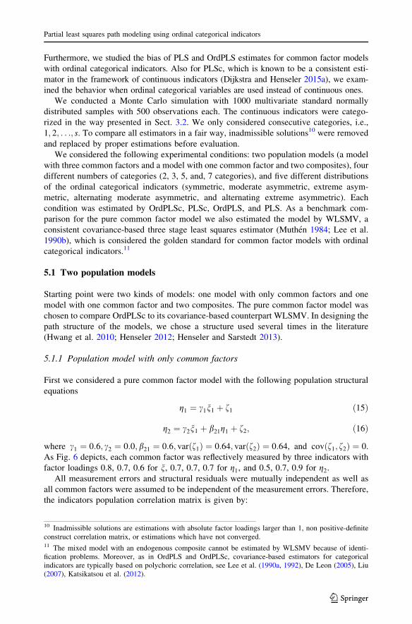
5.1.1 Population model with only common factors

First we considered a pure common factor model with the following population structural

equations

g1 ¼ c1n1 þ f1 ð15Þ

g2 ¼ c2n1 þ b21g1 þ f2; ð16Þ

where c1 ¼ 0:6; c2 ¼ 0:0; b21 ¼ 0:6; varðf1Þ ¼ 0:64; varðf2Þ ¼ 0:64, and covðf1; f2Þ ¼ 0.

As Fig. 6 depicts, each common factor was reflectively measured by three indicators with

factor loadings 0.8, 0.7, 0.6 for n, 0.7, 0.7, 0.7 for g1, and 0.5, 0.7, 0.9 for g2.All measurement errors and structural residuals were mutually independent as well as

all common factors were assumed to be independent of the measurement errors. Therefore,

the indicators population correlation matrix is given by:

10 Inadmissible solutions are estimations with absolute factor loadings larger than 1, non positive-definiteconstruct correlation matrix, or estimations which have not converged.11 The mixed model with an endogenous composite cannot be estimated by WLSMV because of identi-fication problems. Moreover, as in OrdPLS and OrdPLSc, covariance-based estimators for categoricalindicators are typically based on polychoric correlation, see Lee et al. (1990a, 1992), De Leon (2005), Liu(2007), Katsikatsou et al. (2012).

Partial least squares path modeling using ordinal categorical indicators

123

Σ =

⎛⎜⎜⎜⎜⎜⎜⎜⎜⎜⎜⎜⎜⎜⎜⎜⎜⎝

x1 x2 x3 y11 y12 y13 y21 y22 y23

1.0000

0.5600 1.0000

0.4800 0.4200 1.0000

0.3360 0.2940 0.2520 1.0000

0.3360 0.2940 0.2520 0.4900 1.0000

0.3360 0.2940 0.2520 0.4900 0.4900 1.0000

0.1440 0.1260 0.1080 0.2100 0.2100 0.2100 1.0000

0.2016 0.1764 0.1512 0.2940 0.2940 0.2940 0.3500 1.0000

0.2592 0.2268 0.1944 0.3780 0.3780 0.3780 0.4500 0.6300 1.0000

⎞⎟⎟⎟⎟⎟⎟⎟⎟⎟⎟⎟⎟⎟⎟⎟⎟⎠

(17)

5.1.2 Population model with two composites and one common factor

Second, we considered a model with the identical structural model used for the model with

three common factors, but two of the constructs were modeled as composites instead of

common factors. Figure 7 depicts the population model in terms of common and composite

factors. We deliberately chose this representation of the composites and not the one used in

Fig. 2 to clarify the construction of the population correlation matrix of the indicators.

Here n and g1 are constructs modeled as composites. Since the relationship between a

composite and its indicators can be expressed by composite loadings (Fig. 7) or weights,

we also reported the weights: the composites were formed by their connected indicators:

n ¼ x0wx where w0x ¼ ð0:3; 0:5; 0:6Þ and g1 ¼ y1

0wy1 where w0y1¼ ð0:4; 0:5; 0:5Þ. The

common factor g2 was again measured by three indicators with the following loadings: 0.5,

0.7, and 0.9.

x1 x2 x3 y11 y12 y13 y21 y22 y23

ξ η1 η2

ε1 ε2 ε3 δ11 δ12 δ13 δ21 δ22 δ23

ζ1 ζ2

λx1 = .8λx2 = .7

λx3 = .6 λy11 = .7λy12 = .7

λy13 = .7 λy21 = .5λy22 = .7

λy23 = .9

γ1 = .6 β = .6

γ2 = 0

Fig. 6 Population model with three common factors

F. Schuberth et al.

123

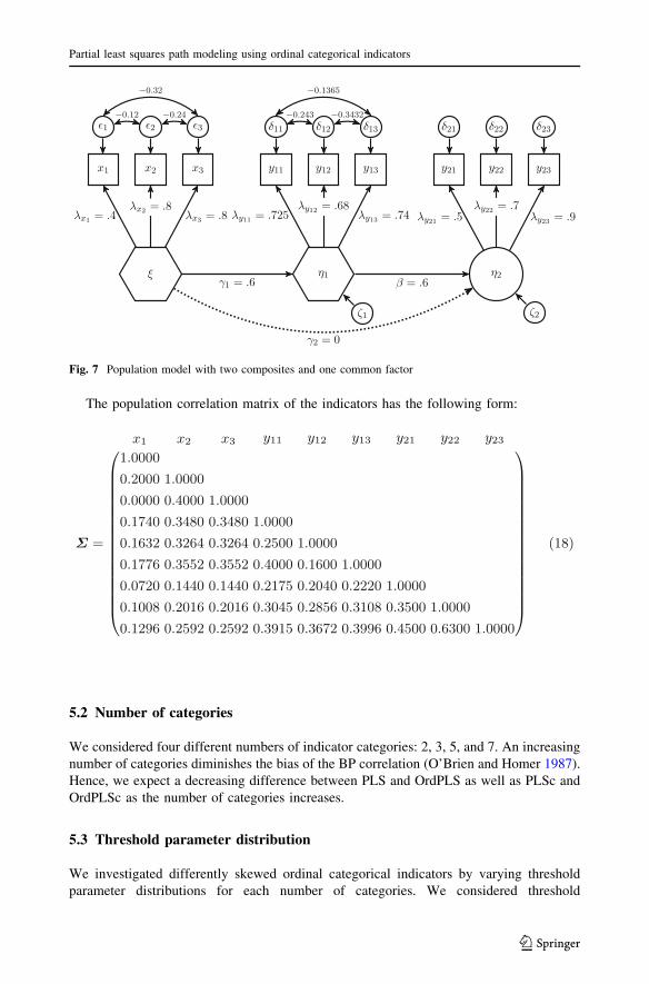
The population correlation matrix of the indicators has the following form:

Σ =

⎛⎜⎜⎜⎜⎜⎜⎜⎜⎜⎜⎜⎜⎜⎜⎜⎜⎝

x1 x2 x3 y11 y12 y13 y21 y22 y23

1.0000

0.2000 1.0000

0.0000 0.4000 1.0000

0.1740 0.3480 0.3480 1.0000

0.1632 0.3264 0.3264 0.2500 1.0000

0.1776 0.3552 0.3552 0.4000 0.1600 1.0000

0.0720 0.1440 0.1440 0.2175 0.2040 0.2220 1.0000

0.1008 0.2016 0.2016 0.3045 0.2856 0.3108 0.3500 1.0000

0.1296 0.2592 0.2592 0.3915 0.3672 0.3996 0.4500 0.6300 1.0000

⎞⎟⎟⎟⎟⎟⎟⎟⎟⎟⎟⎟⎟⎟⎟⎟⎟⎠

(18)

5.2 Number of categories

We considered four different numbers of indicator categories: 2, 3, 5, and 7. An increasing

number of categories diminishes the bias of the BP correlation (O’Brien and Homer 1987).

Hence, we expect a decreasing difference between PLS and OrdPLS as well as PLSc and

OrdPLSc as the number of categories increases.

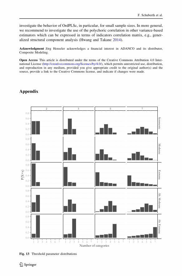
5.3 Threshold parameter distribution

We investigated differently skewed ordinal categorical indicators by varying threshold

parameter distributions for each number of categories. We considered threshold

x1 x2 x3 y11 y12 y13 y21 y22 y23

ξ η1 η2

ε1 ε2 ε3 δ11 δ12 δ13 δ21 δ22 δ23

ζ1 ζ2

λx1 = .4λx2 = .8

λx3 = .8 λy11 = .725λy12 = .68

λy13 = .74 λy21 = .5λy22 = .7

λy23 = .9

γ1 = .6 β = .6

γ2 = 0

−0.12

−0.32

−0.24 −0.243

−0.1365

−0.3432

Fig. 7 Population model with two composites and one common factor

Partial least squares path modeling using ordinal categorical indicators

123

distributions used in the literature before (Rhemtulla et al. 2012): symmetric, moderately

asymmetric, extremely asymmetric, alternating moderately asymmetric, and alternating

extremely asymmetric distributed threshold parameters. In the alternating asymmetric

threshold distribution scenario, the same thresholds were used, but the direction of

asymmetry was reversed for the indicators x2, y11, y13, and y22.12 Since BP correlations are

more downward biased for more asymmetrical threshold distributions (Bollen and Barb

1981; Faber 1988; Holgado-Tello et al. 2010) and even more for alternating skewed

indicators (Olsson 1980), we expect an increasing difference between OrdPLSc and PLSc

estimates as well as OrdPLS and PLS estimates from the symmetrical to the alternating

extreme threshold distribution.

5.4 Data generation and analysis

All simulations were conducted within the R (version 3.2.2) statistical programming

environment (R Core Team 2015). Multivariate standard normally distributed data sets

were drawn using the mvrnorm function of theMASS package (Venables and Ripley 2002).

To obtain PLS and PLSc estimates, we primarily used functions provided by the matrixpls

package (Ronkko 2015), which allows the use of the empirical correlation matrix as input

for PLS and PLSc. A slightly modified version of those functions was also used for

OrdPLS and OrdPLSc. The modified version is provided by the authors upon request.

Since matrixpls is still under development we also partly verified our results obtained with

ADANCO (Henseler and Dijkstra 2015). The polychoric correlation was calculated by the

polychoric function from the psych package (Revelle 2015) using the two-step approach.13

WLSMV estimation was carried out using the lavaan package (Rosseel 2012).

6 Results

This section shows the results of our study.14 In the following, we summarize our findings

in terms of bias with respect to the quality of the parameter estimates for the model

containing only common factors and the mixed model. The bias is the deviation of the

estimated parameter mean across all Monte Carlo simulation runs from its population

counterpart

Bias ¼ 1

1000

X1000

i¼1

hi � h ð19Þ

where h represents the population parameter and h is the estimated parameter. The bias

statistic provides information about the estimators’ unbiasedness and is used as one per-

formance measure to compare OrdPLSc estimates with estimates from approaches com-

monly applied. Moreover, we assessed the estimators’ efficiency in terms of average

12 For an exact description of the threshold parameter distribution, see the Appendix.13 If the polychoric correlation matrix was not positive definite an eigenvector smoothing was done toassure its positive definiteness. Moreover, we followed the recommendation of Savalei (2011) and used the‘ADD’ approach (0.5) for empty cells in the case of two categories and the ‘NONE’ approach else. Thesame was done for WLSMV.14 The complete results are provided in the supplementary material.

F. Schuberth et al.

123

standard deviation across all Monte Carlo simulation runs. We finish by summarizing

inadmissible results, i.e., Heywood cases.

In general, for the moderate asymmetric and the alternating moderate asymmetric

threshold parameter distribution the estimators led to similar results. The same was

observed for extremely and alternating extremely distributed thresholds. For latter con-

ditions, all estimators showed a poorer performance, which confirmed our expectations.

6.1 Bias of the parameter estimates

Figures 8 and 9 display the bias of the path coefficient estimates for b(=0.6) and c2(=0.0),and factor loading estimates for kx1 (=0.5) and ky21 (=0.8) of the pure common factor model

for the different number of categories and the different threshold parameter distributions.

Due to space constraints, we omit the results for the estimated path coefficient c1 and the

other factor loading estimates. They behaved very similar to the ones presented.

These figures make clear that OrdPLSc and WLSMV led to almost the same results for

the estimated path coefficients and factor loadings under all conditions. Both estimators

were hardly biased. Only in case of extremely and alternating extremely skewed indicators

β γ2

−0.3−0.2−0.1

0.00.1

−0.3−0.2−0.1

0.00.1

−0.3−0.2−0.1

0.00.1

−0.3−0.2−0.1

0.00.1

−0.3−0.2−0.1

0.00.1

Symm

etricM

oderateE

xtreme

Alt. M

od.A

lt. Ext.

2 3 5 7 2 3 5 7Number of categories

Bias

Estimator: OrdPLSc WLSMV PLSc OrdPLS PLS

Fig. 8 Model with only common factors: bias for b and c2

Partial least squares path modeling using ordinal categorical indicators

123

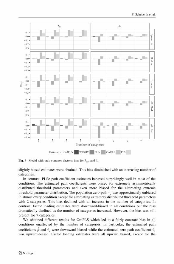
slightly biased estimates were obtained. This bias diminished with an increasing number of

categories.

In contrast, PLSc path coefficient estimates behaved surprisingly well in most of the

conditions. The estimated path coefficients were biased for extremely asymmetrically

distributed threshold parameters and even more biased for the alternating extreme

threshold parameter distribution. The population zero-path c2 was approximately unbiased

in almost every condition except for alternating extremely distributed threshold parameters

with 2 categories. This bias declined with an increase in the number of categories. In

contrast, factor loading estimates were downward-biased in all conditions but the bias

dramatically declined as the number of categories increased. However, the bias was still

present for 7 categories.

We obtained different results for OrdPLS which led to a fairly constant bias in all

conditions unaffected by the number of categories. In particular, the estimated path

coefficients b and c2 were downward-biased while the estimated zero-path coefficient c1was upward-biased. Factor loading estimates were all upward biased, except for the

λy21 λx1

−0.3−0.2−0.1

0.00.1

−0.3−0.2−0.1

0.00.1

−0.3−0.2−0.1

0.00.1

−0.3−0.2−0.1

0.00.1

−0.3−0.2−0.1

0.00.1

Symm

etricM

oderateE

xtreme

Alt. M

od.A

lt. Ext.

2 3 5 7 2 3 5 7Number of categories

Bias

Estimator: OrdPLSc WLSMV PLSc OrdPLS PLS

Fig. 9 Model with only common factors: bias for ky21 and kx1

F. Schuberth et al.

123

estimates of the largest factor loading ky23 ¼ 0:9 which were only slightly biased. This bias

was largely unaffected by the number of categories.

PLS produced the most biased path coefficient estimates for c1 and b1. While the bias of

OrdPLS was fairly constant in all conditions, the bias of the PLS estimates converged to

the bias of the OrdPLS estimates with an increasing number of categories. A similar

pattern was observed for PLS factor loading estimates. For 2 categories, factor loading

estimates were slightly biased, but the bias became more pronounced and converged to the

bias of the OrdPLS factor loading estimates as the number of categories increased.

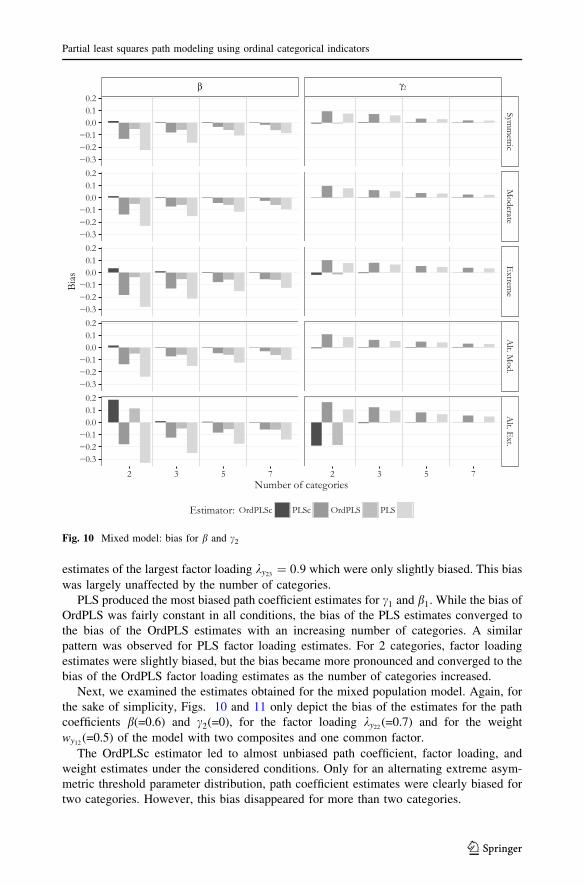
Next, we examined the estimates obtained for the mixed population model. Again, for

the sake of simplicity, Figs. 10 and 11 only depict the bias of the estimates for the path

coefficients b(=0.6) and c2(=0), for the factor loading ky22 (=0.7) and for the weight

wy12 (=0.5) of the model with two composites and one common factor.

The OrdPLSc estimator led to almost unbiased path coefficient, factor loading, and

weight estimates under the considered conditions. Only for an alternating extreme asym-

metric threshold parameter distribution, path coefficient estimates were clearly biased for

two categories. However, this bias disappeared for more than two categories.

β γ2

−0.3−0.2−0.1

0.00.10.2

−0.3−0.2−0.1

0.00.10.2

−0.3−0.2−0.1

0.00.10.2

−0.3−0.2−0.1

0.00.10.2

−0.3−0.2−0.1

0.00.10.2

Symm

etricM

oderateE

xtreme

Alt. M

od.A

lt. Ext.

2 3 5 7 2 3 5 7Number of categories

Bias

Estimator: OrdPLSc PLSc OrdPLS PLS

Fig. 10 Mixed model: bias for b and c2

Partial least squares path modeling using ordinal categorical indicators

123

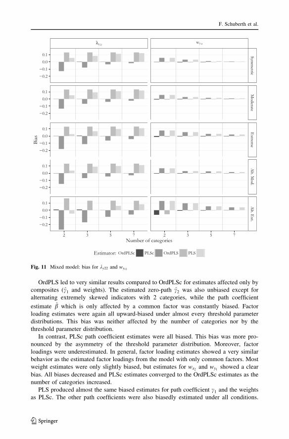
OrdPLS led to very similar results compared to OrdPLSc for estimates affected only by

composites (c1 and weights). The estimated zero-path c2 was also unbiased except for

alternating extremely skewed indicators with 2 categories, while the path coefficient

estimate b which is only affected by a common factor was constantly biased. Factor

loading estimates were again all upward-biased under almost every threshold parameter

distributions. This bias was neither affected by the number of categories nor by the

threshold parameter distribution.

In contrast, PLSc path coefficient estimates were all biased. This bias was more pro-

nounced by the asymmetry of the threshold parameter distribution. Moreover, factor

loadings were underestimated. In general, factor loading estimates showed a very similar

behavior as the estimated factor loadings from the model with only common factors. Most

weight estimates were only slightly biased, but estimates for wx2 and wy1 showed a clear

bias. All biases decreased and PLSc estimates converged to the OrdPLSc estimates as the

number of categories increased.

PLS produced almost the same biased estimates for path coefficient c1 and the weights

as PLSc. The other path coefficients were also biasedly estimated under all conditions.

λy22wy12

−0.2−0.1

0.00.1

−0.2−0.1

0.00.1

−0.2−0.1

0.00.1

−0.2−0.1

0.00.1

−0.2−0.1

0.00.1

Symm

etricM

oderateE

xtreme

Alt. M

od.A

lt. Ext.

2 3 5 7 2 3 5 7Number of categories

Bias

Estimator: OrdPLSc PLSc OrdPLS PLS

Fig. 11 Mixed model: bias for ky22 and wy12

F. Schuberth et al.

123

While this bias decreased with an increasing number of categories, the upward-biased

factor loading estimates became even more biased for an increasing number of categories.

Again, average PLS factor loading estimates tended to converge to OrdPLS average factor

loading estimates.

6.2 Efficiency

Apart from unbiasdness, an estimator’s efficiency is of interest to assess its quality. There-

fore, we evaluated the standard deviations of the standardized path coefficient, loading, and

weight estimates. In general, all standard deviations decreased with an increasing number of

categories, but increased for more asymmetric threshold parameter distributions.

Considering the pure common factor model, WLSMV was always more efficient than

OrdPLSc. Since comparing estimators efficiency is only meaningful for unbiased or

slightly biased estimates, the other results for the pure common factor model are not

evaluated.

Also the estimates for the composite model became more efficient with an increasing

number of categories. For estimated parameters between composites only, PLS and PLSc

as well as OrdPLS and OrdPLSc produced almost the same standard errors. Estimated

parameters connected with at least one common factor showed larger standard deviations

for OrdPLSc than OrdPLS. In most cases, path coefficient and weight estimates were less

efficient for OrdPLS than PLS, while factor loadings were more efficiently estimated by

OrdPLS.

6.3 Inadmissible solutions

We finish the results part by comparing the inadmissible solutions. Inadmissible solutions

are results with absolute factor loadings greater than one, a non positive semi-definite

construct correlation matrix, or results where the estimation algorithm did not converge.

Figure 12 depicts the relative frequencies of inadmissible results.

PLS, OrdPLS, and PLSc produced almost no inadmissible solutions for both kind of

models. In contrast, OrdPLSc and WLSMV produced a few inadmissible solutions under

every condition. The total number of inadmissible results increased for more skewed

distributed indicators. The most inadmissible results were produced for alternating extre-

mely distributed threshold parameters.

A similar pattern was observed for inadmissible results during the bootstrap procedure.

PLS and OrdPLS again produced no improper solutions. In general, the number of inad-

missible results during the bootstrap procedure increased for PLSc with an increasing

number of categories, while it decreased for OrdPLSc and WLSMV.

7 Discussion

The first goal of our study was to propose a variance-based estimator for structural

equation models that is able to consistently estimate models with common factors, com-

posites, and ordinal categorical indicators. We developed OrdPLSc combining the

approaches and thus favorable characteristics of OrdPLS and PLSc.

Our results confirmed that OrdPLSc fulfills its intended purpose. For a sample size of

500 observations, OrdPLSc factor loading, weight, as well as path coefficient estimates

were almost unbiased under every condition. As the combination of the polychoric

Partial least squares path modeling using ordinal categorical indicators

123

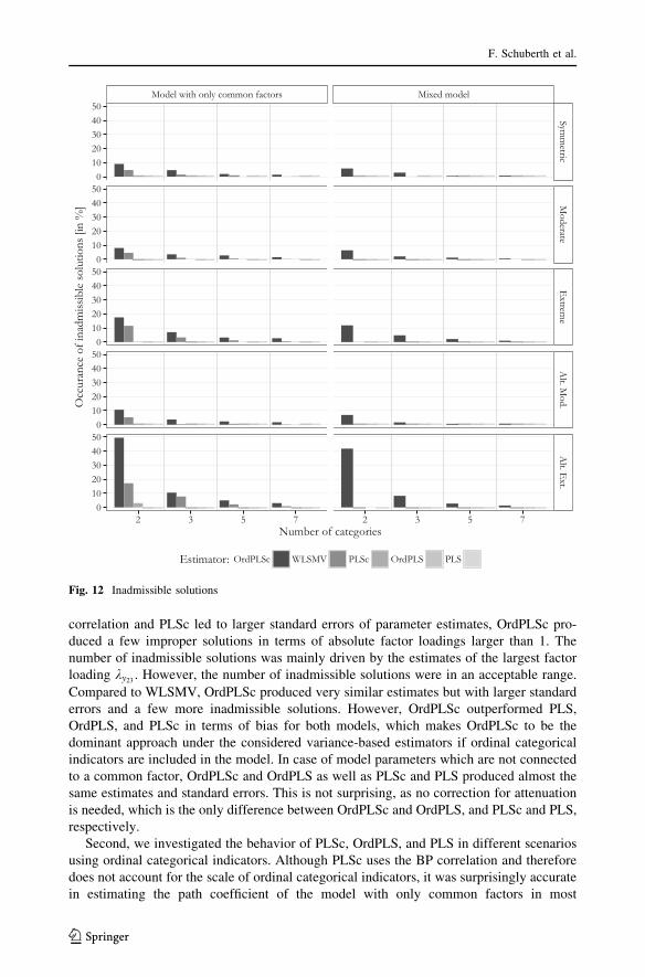
correlation and PLSc led to larger standard errors of parameter estimates, OrdPLSc pro-

duced a few improper solutions in terms of absolute factor loadings larger than 1. The

number of inadmissible solutions was mainly driven by the estimates of the largest factor

loading ky23 . However, the number of inadmissible solutions were in an acceptable range.

Compared to WLSMV, OrdPLSc produced very similar estimates but with larger standard

errors and a few more inadmissible solutions. However, OrdPLSc outperformed PLS,

OrdPLS, and PLSc in terms of bias for both models, which makes OrdPLSc to be the

dominant approach under the considered variance-based estimators if ordinal categorical

indicators are included in the model. In case of model parameters which are not connected

to a common factor, OrdPLSc and OrdPLS as well as PLSc and PLS produced almost the

same estimates and standard errors. This is not surprising, as no correction for attenuation

is needed, which is the only difference between OrdPLSc and OrdPLS, and PLSc and PLS,

respectively.

Second, we investigated the behavior of PLSc, OrdPLS, and PLS in different scenarios

using ordinal categorical indicators. Although PLSc uses the BP correlation and therefore

does not account for the scale of ordinal categorical indicators, it was surprisingly accurate

in estimating the path coefficient of the model with only common factors in most

Model with only common factors Mixed model

01020304050

01020304050

01020304050

01020304050

01020304050

Symm

etricM

oderateE

xtreme

Alt. M

od.A

lt. Ext.

2 3 5 7 2 3 5 7Number of categories

Occ

uran

ce o

f ina

dmiss

ible

solu

tions

[in

%]

Estimator: OrdPLSc WLSMV PLSc OrdPLS PLS

Fig. 12 Inadmissible solutions

F. Schuberth et al.

123

conditions. This could be due to the use of identical threshold parameters for the indicators,

but further research is needed.15 Furthermore, PLSc behaved as expected, factor loadings

were underestimated and the bias increased for more asymmetric threshold parameter

distribution, which is due to the downward-bias of the BP correlation. This bias declined as

the number of categories increased because the bias of the BP correlation decreased.

Therefore, the use of PLSc for models with both common factors and composites is

appropriate but only for indicators with a large number of categories. In our simulation

study, 7 categories were not enough for the bias to disappear completely.

Moreover, our findings support the results of Cantaluppi (2012) that OrdPLS path

coefficient estimates are less biased than PLS estimates in the pure common factor model.

Although it takes into account the scale of ordinal categorical indicators, the problem of

attenuation remains unaddressed which led to downward-biased estimated path coefficients

and upward-biased estimated factor loadings. As this bias was almost unaffected by the

number of categories and the indicators’ distribution, OrdPLS estimates were constantly

biased. However, OrdPLS accurately estimated the model parameters which were not

connected to common factors because no correction for attenuation is needed. Therefore,

OrdPLS is an appropriate estimator for models containing only constructs modeled as

composites.

Traditional PLS suffers from two shortcomings: no correction for attenuation in case of

common factors and not accounting for the scale of ordinal categorical indicators. For a

small number of categories the bias of attenuation and the bias of the BP correlation

cancelled out, which led to only slightly biased factor loading estimates. When the number

of categories increased, the bias of the BP correlation decreased and PLS factor loading

estimates became more and more inaccurate and converged to the OrdPLS estimates,

which do not suffer from the bias of the BP correlation. Therefore, PLS should be cau-

tiously used for models containing common factors regardless whether ordinal categorical

indicators are included or not.

Since OrdPLSc uses the polychoric correlation which assumes normality for the latent

variables underlying each ordinal categorical indicator, it cannot be declared anymore as

an approach which is free of distributional assumptions. However, the assumption of joint

normality of the underlying unobservable variables can be relaxed, as the polychoric

correlation produces fairly unbiased correlation estimates for elliptically symmetric dis-

tributed variables (Kukuk 1999). Furthermore, due to the nature of the ordinal categorical

indicators, point estimates of factor scores or composite scores should not be directly

calculated from their observations. To overcome this shortcoming procedures like the

mode estimation, median estimation, or mean estimation can be used (Cantaluppi 2012).

This issue currently limits the use of OrdPLSc for prediction.16

In our simulation study, we only considered situations where all indicators were mea-

sured on an ordinal categorical scale. In empirical research practice, continuous indicators

are often included in the model. In such a situation, the polyserial or BP correlation should

be used, too, to estimate the population correlation matrix. Future research should inves-

tigate the behavior of OrdPLSc for models containing a mixture of ordinal categorical and

continuous indicators. As a study is limited to its design, we further recommend to

15 Since the BP correlation is about to be proportional biased (for a certain range of correlations, see Kukuk1991), bias cancels out for path coefficients and only affects factor loading and correction factor estimates.Results may change for indicators with a different number of categories and different threshold parameterdistribution.16 This issue is subject of current research by Florian Schuberth and Gabriele Cantaluppi.

Partial least squares path modeling using ordinal categorical indicators

123

investigate the behavior of OrdPLSc, in particular, for small sample sizes. In more general,

we recommend to investigate the use of the polychoric correlation in other variance-based

estimators which can be expressed in terms of indicators correlation matrix, e.g., gener-

alized structural component analysis (Hwang and Takane 2014).

Acknowledgment Jorg Henseler acknowledges a financial interest in ADANCO and its distributor,Composite Modeling.

Open Access This article is distributed under the terms of the Creative Commons Attribution 4.0 Inter-national License (http://creativecommons.org/licenses/by/4.0/), which permits unrestricted use, distribution,and reproduction in any medium, provided you give appropriate credit to the original author(s) and thesource, provide a link to the Creative Commons license, and indicate if changes were made.

Appendix

2 3 5 7

0.0

0.2

0.4

0.6

0.8

0.0

0.2

0.4

0.6

0.8

0.0

0.2

0.4

0.6

0.8

0.0

0.2

0.4

0.6

0.8

0.0

0.2

0.4

0.6

0.8

Symm

etricM

oderateE

xtreme

Alt. M

oderateA

lt. Extrem

e

1 2 3 4 5 6 7 1 2 3 4 5 6 7 1 2 3 4 5 6 7 1 2 3 4 5 6 7Number of categories

P(X

=x)

Fig. 13 Threshold parameter distributions

F. Schuberth et al.

123

References

Albers, S.: PLS and success factor studies in marketing. In: Esposito, V.V., Chin, W.W., Henseler, J., Wang,H. (eds.) Handbook of Partial Least Squares, pp. 409–425. Springer, Berlin (2010)

Betzin, J., Henseler, J.: Looking at the antecedents of perceived switching costs. A PLS path modelingapproach with categorical indicators, Barcelona, Spain (2005)

Bollen, K.A., Barb, K.H.: Pearson’s r and coarsely categorized measures. Am. Sociol. Rev. 46, 232–239(1981)

Bollen, K.A., Bauldry, S.: Three Cs in measurement models: causal indicators, composite indicators, andcovariates. Psychol. Methods 16(3), 265 (2011)

Cantaluppi, G.: A partial least squares algorithm handling ordinal variables also in presence of a smallnumber of categories (2012). arXiv preprint arXiv:12125049

Cantaluppi, G., Boari, G.: A partial least squares algorithm handling ordinal variables. In: Saporta, G.,Russolillo, G., Trinchera, L., Abdi H, Esposito V.V. (eds.) The Multiple Facets of Partial Least SquaresMethods: PLS, Paris, France, 2014, Springer (2016)

Carroll, J.B.: The nature of the data, or how to choose a correlation coefficient. Psychometrika 26(4),347–372 (1961)

Coelho, P.S., Esteves, S.P.: The choice between a five-point and a ten-point scale in the framework ofcustomer satisfaction measurement. Int. J. Market Res. 49(3), 313–339 (2007)

Cohen, J., Cohen, P., West, S.G., Aiken, L.S.: Applied Multiple Regression/Correlation Analysis for theBehavioral Sciences. Routledge, New York (2013)

De Leon, A.: Pairwise likelihood approach to grouped continuous model and its extension. Stat. Probab.Lett. 75(1), 49–57 (2005)

Dijkstra T.K.: Latent variables in linear stochastic models: Reflections on ‘‘Maximum Likelihood’’ and‘‘Partial Least Squares’’ methods (PhD thesis 1981, 2nd ed. 1985). The Netherlands: SociometricResearch Foundation, Amsterdam (1985)

Dijkstra, T.K.: Some comments on maximum likelihood and partial least squares methods.J. Econom. 22(1), 67–90 (1983)

Dijkstra, T.K.: Latent variables and indices: Herman Wold’s basic design and partial least squares. In:Esposito, V.V., Chin, W.W., Henseler, J., Wang, H. (eds.) Handbook of Partial Least Squares,pp. 23–46. Springer, New York (2010)

Dijkstra, T.K.: Consistent partial least squares estimators for linear and polynomial factor models. A reportof a belated, serious and not even unsuccessful attempt. ResearchGate (2011). doi:10.13140/RG.2.1.3997.0405 (Unpublished Manuscript)

Dijkstra, T.K., Schermelleh-Engel, K.: Consistent partial least squares for nonlinear structural equationmodels. Psychometrika 79(4), 585–604 (2014)

Dijkstra, T.K., Henseler, J.: Consistent and asymptotically normal PLS estimators for linear structuralequations. Comput. Stat. Data Anal. 81, 10–23 (2015a)

Dijkstra, T.K., Henseler, J.: Consistent partial least squares path modeling. MIS Q. 39(2), 297–316 (2015b)Drasgow, F.: Polychoric and polyserial correlations. Encycl. Stat. Sci. 7, 68–74 (1988)Faber, J.: Consistent estimation of correlations between observed interval variables with skewed distribu-

tions. Qual. Quant. 22(4), 381–392 (1988)Fornell, C., Bookstein, F.L.: Two structural equation models: LISREL and PLS applied to consumer exit-

voice theory. J. Mark. Res. 19(4), 440–452 (1982)Hair, J.F., Ringle, C.M., Sarstedt, M.: PLS-SEM: indeed a silver bullet. J. Mark. Theory Pract. 19(2),

139–152 (2011)Hair, J.F., Sarstedt, M., Ringle, C.M., Mena, J.A.: An assessment of the use of partial least squares structural

equation modeling in marketing research. J. Acad. Mark. Sci. 40(3), 414–433 (2012)Henseler, J.: Why generalized structured component analysis is not universally preferable to structural

equation modeling. J. Acad. Mark. Sci. 40(3), 402–413 (2012)Henseler, J., Dijkstra, T.K.: ADANCO 2.0 (2015). www.composite-modeling.comHenseler, J., Sarstedt, M.: Goodness-of-fit indices for partial least squares path modeling. Comput. Stat.

28(2), 565–580 (2013)Henseler, J., Dijkstra, T.K., Sarstedt, M., Ringle, C.M., Diamantopoulos, A., Straub, D.W., Ketchen, D.J.,

Hair, J.F., Hult, G.T.M., Calantone, R.J.: Common beliefs and reality about PLS comments on Ronkkoand Evermann (2013). Organ. Res. Methods 28(1), 1094428114526,928 (2014)

Henseler, J., Ringle, C.M., Sarstedt, M.: A new criterion for assessing discriminant validity in variance-based structural equation modeling. J. Acad. Mark. Sci. 43(1), 1–21 (2015)

Partial least squares path modeling using ordinal categorical indicators

123

Holgado-Tello, F.P., Chacon-Moscoso, S., Barbero-Garcıa, I., Vila-Abad, E.: Polychoric versus Pearsoncorrelations in exploratory and confirmatory factor analysis of ordinal variables. Qual. Quant. 44(1),153–166 (2010)

Hook, K., Lowgren, J.: Strong concepts: Intermediate-level knowledge in interaction design research. ACMTrans. Comput. Hum. Interact (TOCHI) 19(3), 23 (2012)

Hwang, H., Takane, Y.: Generalized Structured Component Analysis: A Component-Based Approach toStructural Equation Modeling. CRC Press, Boca Raton (2014)

Hwang, H., Malhotra, N.K., Kim, Y., Tomiuk, M.A., Hong, S.: A comparative study on parameter recoveryof three approaches to structural equation modeling. J. Mark. Res. 47(4), 699–712 (2010)

Jakobowicz, E., Derquenne, C.: A modified PLS path modeling algorithm handling reflective categoricalvariables and a new model building strategy. Comput. Stat. Data Anal. 51(8), 3666–3678 (2007)

Katsikatsou, M., Moustaki, I., Yang-Wallentin, F., Joreskog, K.G.: Pairwise likelihood estimation for factoranalysis models with ordinal data. Comput. Stat. Data Anal. 56(12), 4243–4258 (2012)

Kettenring, J.R.: Canonical analysis of several sets of variables. Biometrika 58(3), 433–451 (1971)Ketterlinus, R.D., Bookstein, F.L., Sampson, P.D., Lamb, M.E.: Partial least squares analysis in develop-

mental psychopathology. Dev. Psychopathol. 1(04), 351–371 (1989)Kukuk. M.: Latente Strukturgleichungsmodelle und rangskalierte Daten. Hartung-Gorre (1991)Kukuk, M.: Analyzing ordered categorical data derived from elliptically symmetric distributions. Allge-

meines Statistisches Archiv. 83, 308–323 (1999)Lee, S.Y., Poon, W.Y.: Two-step estimation of multivariate polychoric correlation. Commun. Stat. Theory

Methods 16(2), 307–320 (1987)Lee, S.Y., Poon, W.Y., Bentler, P.M.: Full maximum likelihood analysis of structural equation models with

polytomous variables. Stat. Probab. Lett. 9(1), 91–97 (1990a)Lee, S.Y., Poon, W.Y., Bentler, P.M.: A three-stage estimation procedure for structural equation models

with polytomous variables. Psychometrika 55(1), 45–51 (1990b)Lee, S.Y., Poon, W.Y., Bentler, P.M.: Structural equation models with continuous and polytomous variables.

Psychometrika 57(1), 89–105 (1992)Liu, J.: Multivariate Ordinal Data Analysis with Pairwise Likelihood and Its Extension to SEM. PhD thesis,

University of California Los Angeles (2007)Lohmoller, J.B.: Latent Variable Path Modeling with Partial Least Squares. Springer, Berlin (2013)Maraun, M.D., Halpin, P.F.: Manifest and latent variates. Measurement 6(1–2), 113–117 (2008)Marcoulides, G.A., Saunders, C.: Editor’s comments: PLS: a silver bullet? MIS Q. 30(2), iii-ix (2006)McDonald, R.P.: Path analysis with composite variables. Multivar. Behav. Res. 31(2), 239–270 (1996)Muthen, B.: A general structural equation model with dichotomous, ordered categorical, and continuous

latent variable indicators. Psychometrika 49(1), 115–132 (1984)Noonan, R., Wold, H.: PLS path modeling with indirectly observed variables. In: Joreskog, K.G., Wold, H.

(eds.) Systems under Indirect Observation: Causality, Structure, Prediction Part II. North-Holland,Amsterdam (1982)

O’Brien, R.M., Homer, P.: Corrections for coarsely categorized measures: LISREL’s polyserial and poly-choric correlations. Qual. Quant. 21(4), 349–360 (1987)

Olsson, U.: Maximum likelihood estimation of the polychoric correlation coefficient. Psychometrika 44(4),443–460 (1979)

Olsson, U.: Measuring of correlation in ordered two-way contingency tables. J. Mark. Res. 391–394 (1980)Olsson, U., Drasgow, F., Dorans, N.J.: The polyserial correlation coefficient. Psychometrika 47(3), 337–347

(1982)Pearson, K.: Mathematical contributions to the theory of evolution. VII. On the correlation of characters not

quantitatively measurable. Philos. Trans. R. Soc. Lond. Ser. A Contain. Papers Math. Phys. Char. 195,1–405 (1900)

Pearson, K.: On the measurement of the influence of ‘‘broad categories’’ on correlation. Biometrika 9(1/2),116–139 (1913)

Poon, W.Y., Lee, S.Y.: Maximum likelihood estimation of multivariate polyserial and polychoric correla-tion coefficients. Psychometrika 52(3), 409–430 (1987)

Quiroga, A.M.: Studies of the polychoric correlation and other correlation measures for ordinal variables.PhD thesis, Uppsala University (1992)

R Core Team: R: a language and environment for statistical computing. R Foundation for StatisticalComputing, Vienna (2015). https://www.R-project.org/

Revelle, W.: Psych: procedures for psychological, psychometric, and personality research. NorthwesternUniversity, Evanston, Illinois (2015). http://CRAN.R-project.org/package=psych, R package version 1.5.6

F. Schuberth et al.

123

Rhemtulla, M., Brosseau-Liard, P.E., Savalei, V.: When can categorical variables be treated as continuous?A comparison of robust continuous and categorical SEM estimation methods under suboptimal con-ditions. Psychol. Methods 17(3), 354–373 (2012)

Rigdon, E.E.: Rethinking partial least squares path modeling: In praise of simple methods. Long Range Plan.45(5), 341–358 (2012)

Ringle, C.M., Sarstedt, M., Straub, D.: A critical look at the use of PLS-SEM in MIS Quarterly. MIS Q.36(1) (2012)

Ronkko, M.: matrixpls: matrix-based partial least squares estimation (2015). https://github.com/mronkko/matrixpls, R package version 0.6.0

Rosseel, Y.: lavaan: an R package for structural equation modeling. J. Stat. Softw. 48(2):1–36 (2012). http://www.jstatsoft.org/v48/i02/

Russolillo, G.: Non-metric partial least squares. Electron. J. Stat. 6, 1641–1669 (2012)Savalei, V.: What to do about zero frequency cells when estimating polychoric correlations. Struct. Equ.

Model. 18(2), 253–273 (2011)Schneeweiss, H.: Consistency at Large in Models with Latent Variables. Elsevier, Amsterdam (1993)Tenenhaus, M.: Component-based structural equation modelling. Total Qual. Manag. 19(7–8), 871–886

(2008)Tenenhaus, M., Vinzi, V.E., Chatelin, Y.M., Lauro, C.: PLS path modeling. Comput. Stat. Data Anal. 48(1),

159–205 (2005)Trygg, J., Wold, S.: Orthogonal projections to latent structures (O-PLS). J. Chemom. 16(3), 119–128 (2002)Venables W.N., Ripley, B.D.: Modern Applied Statistics with S, 4th edn. Springer, New York (2002)Wold, H.: Path Models with Latent Variables: The NIPALS Approach. Academic Press, Cambridge (1975)Wold, H.: Soft modeling: The basic design and some extensions. In: Joreskog, K.G., Wold, H. (eds.)

Systems Under Indirect Observations, Part II, Chapter I, pp. 1–54. North-Holland, Amsterdam (1982)Wooldridge, J.: Introductory econometrics: A modern approach. Cengage Learning (2012)Wylie, P.B.: Effects of coarse grouping and skewed marginal distributions on the Pearson product moment

correlation coefficient. Educ. Psychol. Measur. 36(1), 1–7 (1976)Young, F.W.: Quantitative analysis of qualitative data. Psychometrika 46(4), 357–388 (1981)Yule, G.U.: On the association of attributes in statistics: With illustrations from the material of the

Childhood Society, & c. Philos. Trans. R. Soc. Lond. Ser. A Contain. Papers Math. Phys. Char. 194,257–319 (1900)

Partial least squares path modeling using ordinal categorical indicators

123