Congressional Budget Office

National Tax Association49th Annual Spring Symposium

May 16, 2019

Kerk PhillipsMacroeconomic Analysis Division

Overlapping Generations Model Roundtable: Model Comparisons From a Stylized

Social Security Experiment

1

CBO

CBO’s Symposium in December 2018

The Congressional Budget Office held a symposium about overlapping generations (OLG) models in December 2018. Its objectives:

To learn more about existing OLG models used for fiscal policy analysis, and

To learn more about the effects of a reduction in Old-Age and Survivors Insurance (OASI) benefits.

2

CBO

OLG Models

The models examined at the symposium were the following:

Congressional Budget Office Model

Diamond-Zodrow Model

EY QUEST Model

Global Gaidar Model

JCT In-House Model

OG-USA Model

Penn Wharton Budget Model

3

CBO

The Structure of OLG Models

OLG models are used to analyze the effects of fiscal policy on households’ decisions to work and save; the distribution of income, wealth, consumption, and taxes among households; and the well-being of different generations.

The models differ, but they all have the following four components:

Households, which differ by income, wealth, and age, and which choose how much to work and save;

Firms, which purchase households’ labor and rent capital to maximize profits;

Government, which collects taxes from a variety of sources and spends resources on public programs, such as Social Security’s OASI program; and

The rest of the world, which interacts with the domestic economy through financial markets.

4

CBO

The Structure of Households Over Time

In each period, a new cohort of households is born. Within each cohort, households differ by income, wealth, and other characteristics, depending on the model.

5

CBO

The OLG Models’ Key Differences

The OLG models that CBO examined differ in various ways, including these:

Their degree of openness to the rest of the world;

Their use of demographics (such as aging and migration);

The way they structure the OASI program;

The way they treat taxation;

The interest rate they use for payments on government debt; and

The nature, timing, and target of their “closure rule”—that is, a policy change that stabilizes the ratio of debt to gross domestic product (GDP) in the long run.

6

CBO

Whether the benefit reductions are modeled as anticipated or unanticipated does not appear to change the long-run results significantly.

The degree of openness to foreign capital is critical. The assumption of a large, open economy is preferred when modeling the United States.

Harmonizing the dates of the closure and of the policy used is important.

Lessons Learned From the December Symposium

7

CBO

CBO conducted an experiment in which the various OLG models were used to estimate what would happen if OASI benefits were reduced evenly by one-third in 2031. In that experiment:

Benefits are reduced for all current and future recipients, and no generation is exempt from the reduction in benefits—that is, there is no grandfathering.

The reductions are announced in 2018, so households fully anticipate that they will arrive in 2031.

The closure rule is that beginning in 2050, noninvestment government spending (or lump-sum transfers) is decreased—so the debt-to-GDP ratio is stabilized from 2050 onward.

Key Features of the Stylized Social Security Experiment

8

CBO

The following results are intended solely to show how the models compare with each other. Both the scenario and the closure rule are highly stylized, so none of these results should be interpreted as forecasts or projections by any of the participating modelers.

An Important Caveat

9

CBO

Effect on Debt-to-GDP Ratio in the Models

Reducing OASI benefits reduces the debt-to-GDP ratio by about 55 to 65 percentage points in the long run in most models.

The GGM model finds a larger reduction in the debt-to-GDP ratio.

Percentage Points

10

CBO

Effect on Capital Stock in the Models

The capital stock increases in relation to the baseline. The results are sensitive to the models’ structure and calibration strategy.

Percent

11

CBO

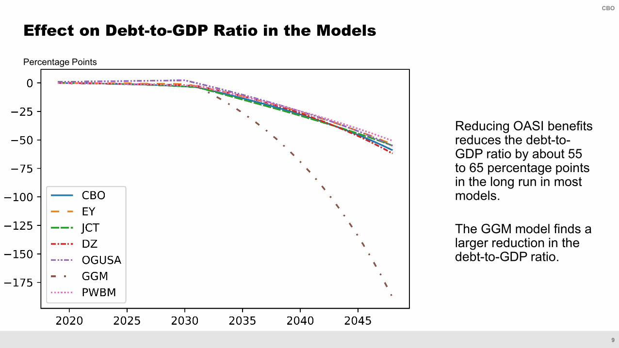
Effect on Labor Force in the Models

The short-run labor supply increases modestly in most models.

Percent

12

CBO

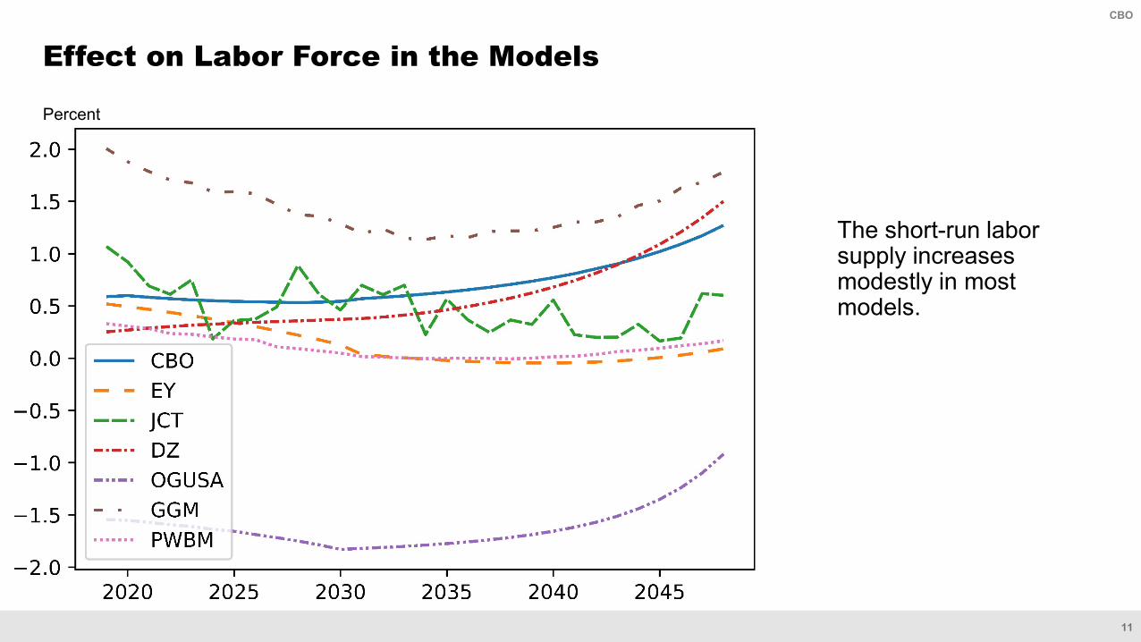
Effect on GDP in the Models

GDP follows the models’ paths for capital and labor.

Percent

13

CBO

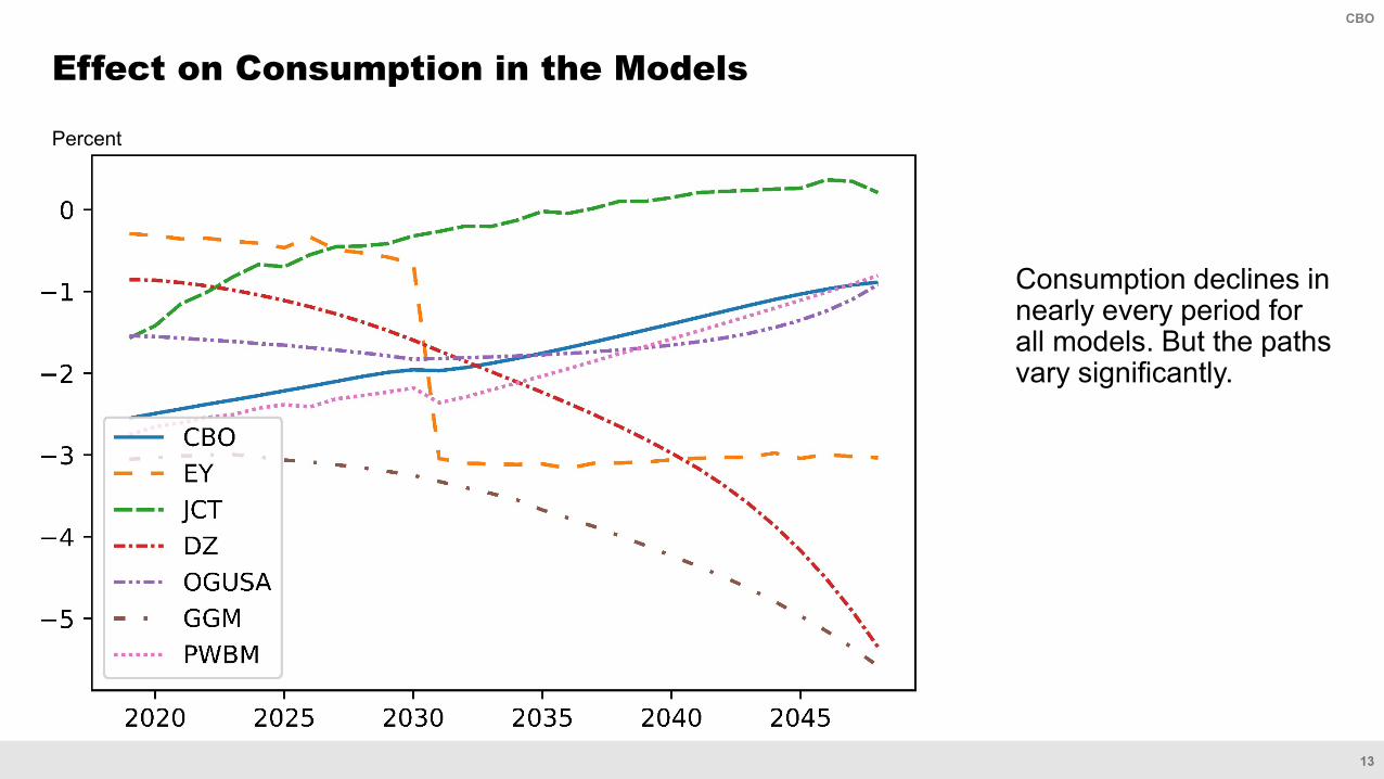
Effect on Consumption in the Models

Consumption declines in nearly every period for all models. But the paths vary significantly.

Percent

14

CBO

Effect on Wages in the Models

Wages increase in most models, but a few models generate lower wages in the near term.

Percent

15

CBO

The interest rates are for nongovernment financial assets.

Effect on Interest Rates in the Models

Interest rates fall in most models and in nearly every period.

Percentage Points

16

CBO

What are the models’ principal differences and similarities? Where do we find common ground, and how large are the differences?

What features of the models drive the different results? (Recall the key differences described earlier—the models’ treatment of the openness of the economy, demographics, the OASI program’s structure, taxation, interest rates, and the closure rule.)

What are the models’ limitations? Given those limitations, do the models still help us understand the issues?

What are the effects on households’ well-being? How should we interpret the results in the context of our assumptions about the closure rule?

Areas for Further Discussion

17

CBO

Documentation of OLG Models

Congressional Budget Office Model: Congressional Budget Office, “An Overview of CBO’s Life-Cycle Growth Model” (February 2019),

www.cbo.gov/publication/54985. Shinichi Nishiyama and Felix Reichling, The Costs to Different Generations of Policies That Close

the Fiscal Gap, Working Paper 2015-10 (Congressional Budget Office, December 2015), www.cbo.gov/publication/51097.

Diamond-Zodrow Model: George R. Zodrow and John W. Diamond, “Dynamic Overlapping Generations Computable General Equilibrium Models and the Analysis of Tax Policy: The Diamond-Zodrow Model,” in Peter B. Dixon and Dale W. Jorgensen, eds., Handbook of Computable General Equilibrium Modeling (Elsevier, 2013), vol. 1, pp. 743–813, https://doi.org/10.1016/B978-0-444-59568-3.00011-0.

EY QUEST Model: EY, Analyzing the Macroeconomic Impacts of the Tax Cuts and Jobs Act on the US Economy and Key Industries (2018), https://tinyurl.com/y4fpbjgf (PDF, 2.9 MB).

18

CBO

Documentation of OLG Models (Continued)

Global Gaidar Model: Seth G. Benzell, Laurence J. Kotlikoff, and Guillermo LaGarda, Simulating Business Cash Flow Taxation: An Illustration Based on the “Better Way” Corporate Tax Reform, Working Paper 23675 (National Bureau of Economic Research, August 2017), www.nber.org/papers/w23675.

JCT In-House Model: Rachel Moore and Brandon Pecoraro, “Modeling the Internal Revenue Code in a Heterogeneous-

Agent Framework: An Application to TCJA” (draft, May 2019), https://doi.org/10.2139/ssrn.3367192.

Rachel Moore and Brandon Pecoraro, “Macroeconomic Implications of Modeling the Internal Revenue Code in a Heterogeneous-Agent Framework” (draft, December 2018), https://doi.org/10.2139/ssrn.3193142.

19

CBO

Documentation of OLG Models (Continued)

OG-USA Model: Richard W. Evans and Jason DeBacker, “OG-USA: Documentation for the Large-Scale Dynamic General Equilibrium Overlapping Generations Model for U.S. Policy Analysis” (November 2018), https://tinyurl.com/y694ljom (PDF, 1.6 MB).

Penn Wharton Budget Model: Penn Wharton Budget Model, Penn Wharton Budget Model: Dynamic OLG Model (January 2019), www.budgetmodel.wharton.upenn.edu/dynamic-olg/.