OVERLAPPING GENERATIONS MODELS OF GENERAL EQUILIBRIUM

By

John Geanakoplos

May 2008

COWLES FOUNDATION DISCUSSION PAPER NO. 1663

COWLES FOUNDATION FOR RESEARCH IN ECONOMICS YALE UNIVERSITY

Box 208281 New Haven, Connecticut 06520-8281

http://cowles.econ.yale.edu/

Overlapping Generations Models of GeneralEquilibrium

John Geanakoplos

July 3, 2007

Abstract

The OLG model of Allais and Samuelson retains the methodological as-sumptions of agent optimization and market clearing from the Arrow-Debreumodel, yet its equilibrium set has different properties: Pareto inefficiency, inde-terminacy, positive valuation of money, and a golden rule equilibrium in whichthe rate of interest is equal to population growth (independent of impatience).These properties are shown to derive not from market incompleteness, butfrom lack of market clearing "at infinity;" they can be eliminated with land oruniform impatience. The OLG model is used to analyze bubbles, social secu-rity, demographic effects on stock returns, the foundations of monetary theory,Keynesian vs. real business cycle macromodels, and classical vs. neoclassicaldisputes.Key words: demography, inefficiency, indeterminacy, money, bubbles, cy-

cles, rate of interest, impatience, land, infinity, expectations, social security,golden rule.JEL classification: D1, D3, D5, D6, D9, E11, E12, E13, E2, E3, E4, E6

The consumption loan model that Paul Samuelson introduced in 1958 to analyzethe rate of interest, with or without the social contrivance of money, has developedinto what is without doubt the most important and influential paradigm in neoclassi-cal general equilibrium theory outside of the Arrow—Debreu economy. Earlier MauriceAllais (1947) had presented similar ideas which unfortunately did not then receivethe attention they deserved. A vast literature in public finance and macroeconomicsis based on the model, including studies of the national debt, social security, theincidence of taxation and bequests on the accumulation of capital, the Phillips curve,the business cycle, and the foundations of monetary theory. In the following pages Igive a hint of these myriad applications only in so far as they illuminate the generaltheory. My main concern is with the relationship between the Samuelson model andthe Arrow—Debreu model.Allais’ and Samuelson’s innovation was in postulating a demographic structure

in which generations overlap, indefinitely into the future; up until then it had been

1

customary to regard all agents as contemporaneous. In the simplest possible example,in which each generation lives for two periods, endowed with a perishable commoditywhen young and nothing when old, Samuelson noticed a great surprise. Althougheach agent could be made better off if he gave half his youthful birthright to hispredecessor, receiving in turn half from his successor, in the marketplace there wouldbe no trade at all. A father can benefit from his son’s resources, but has nothing tooffer in return.This failure of the market stirred a long and confused controversy. Samuelson

himself attributed the suboptimality to a lack of double coincidence of wants. Hesuggested the social contrivance of money as a solution. Abba Lerner suggestedchanging the definition of optimality. Others, following Samuelson’s hints aboutthe financial intermediation role of money, sought to explain the consumption loanmodel by the incompleteness of markets. It has only gradually become clear that the“Samuelson suboptimality paradox” has nothing to do with the absence of markets orfinancial intermediation. Exactly the same equilibrium allocation would be reachedif all the agents, dead and unborn, met (in spirit) before the beginning of time andtraded all consumption goods, dated from all time periods, simultaneously underthe usual conditions of perfect intermediation. Indeed, almost 100 years ago IrvingFisher implicitly argued that any sequential economy without uncertainty, but witha functioning loan market, could be equivalently described as if all markets met oncewith trade conducted at present value prices.Over the years Samuelson’s consumption loan example, infused with Arrow—

Debreu methods, has been developed into a full blown general equilibrium modelwith many agents, multiple kinds of commodities and production. It is equally faith-ful to the neoclassical methodological assumptions of agent optimization, marketclearing, price taking, and rational expectations as the Arrow—Debreu model. Thismore comprehensive version of Samuelson’s original idea is known as the overlappinggenerations (OLG) model of general equilibrium.Despite the methodological similarities between the OLG model and the Arrow—

Debreu model, there is a profound difference in their equilibria. The OLG equilibriamay be Pareto suboptimal. Money may have positive value. There are robust OLGeconomies with a continuum of equilibria. Indeed, the more commodities per period,the higher the dimension of multiplicity may be. Finally, the core of an OLG economymay be empty. None of this could happen in any Arrow—Debreu economy.The puzzle is why? One looks in vain for an externality, or one of the other

conventional pathologies of an Arrow—Debreu economy. It is evident that the simplefact that generations overlap cannot be an explanation, since by judicious choiceof utility functions one can build that into the Arrow—Debreu model. It cannot besimply that the time horizon is infinite, as we shall see, since there are classes of infinitehorizon economies whose equilibria behave very much like Arrow—Debreu equilibria.It is the combination, that generations overlap indefinitely, which is somehow crucial.In Section 4 I explain how.

2

Note that in the Arrow—Debreu economy the number of commodities, and henceof time periods, is finite. One is tempted to think that if the end of the world is putfar enough off into the future, it could hardly matter to behavior today. But recallingthe extreme rationality hypotheses of the Arrow—Debreu model, it should not besurprising that such a cataclysmic event, no matter how long delayed, could exercisea strong influence on behavior. Indeed the OLG model proves that it does. One canthink of other examples. Social security, based on the pay-as-you-go principle in theUnited States in which the young make payments directly to the old, depends cruciallyon people thinking that there might always be a future generation. Otherwise thelast generation of young will not contribute; foreseeing that, neither will the secondto last generation of young contribute, nor, working backward, will any generationcontribute. Another similar example comes from game theory, in which cooperationdepends on an infinite horizon. On the whole, it seems at least as realistic to supposethat everyone believes the world is immortal as to suppose that everyone believes ina definite date by which it will end. (In fact, it is enough that people believe, forevery T , that there is positive probability the world lasts past T .)In Section 1, I analyze a simple one-commodity OLG model from the present

value general equilibrium perspective. This illustrates the paradoxical nature of OLGequilibria in the most orthodox setting. These paradoxical properties can hold equallyfor economies with many commodities, as pointed out in Section 4. Section 2 discussesthe possibility of equilibrium cycles in a one-commodity, stationary, OLG economy.In Section 3, I describe OLG equilibria from a sequential markets point of view, andshow that money can have positive value.In the simple OLG economy of Section 1 there are two steady state equilibria,

and a continuum of nonstationary equilibria. Out of all of these, only one is Paretoefficient, and it has the property that the real rate of interest is always zero, just equalto the rate of population growth, independent of the impatience of the consumersor the distribution of endowments between youth and old age. This “golden rule”equilibrium seems to violate Fisher’s impatience theory of interest.In Section 5 I add land to the one-commodity model of Section 1. It turns out that

now there is a unique steady state equilibrium, that is Pareto efficient, and that has arate of interest greater than the population growth rate, that increases if consumersbecome more impatient. Land restores Fisher’s view of interest. In this setting it isalso possible to analyze the effects of social security.In Section 6 I briefly introduce variations in demography. It is well known that

birth rates in the United States have oscillated every twenty years over the last cen-tury. Stock prices have curiously moved in parallel, rising rapidly from 1945—65,falling from 65—85, and rising ever since. One might therefore expect stock pricesto fall as the current baby boom generation retires. But some authors have claimedthat the parallel trending of stock prices must be coincidental. Otherwise, sincedemographic changes are known long in advance, rational investors would have an-ticipated the stock trends and changed them. In Section 6 I allow the size of the

3

generations to alternate and confirm that in OLG equilibrium, land prices rise andfall with demography, even though the changes are perfectly anticipated.In Section 7 I show that not just land, but also uniform impatience restores

the properties of infinite horizon economies to those found in finite Arrow Debreueconomies.Section 8 takes up the question of comparative statics. If there is a multiplicity of

OLG equilibria, what sense can be made of comparative statics? Section 8 summarizesthe work showing that for perfectly anticipated changes, there is only one equilibriumin the multiplicity that is “near” an original “regular” equilibrium. For unanticipatedchanges, there may be a multidimensional multiplicity. But it is parameterizable.Hence by always fixing the same variables, a unique prediction can be made forchanges in the equilibrium in response to perturbations. In Section 9 we see how thiscould be used to understand some of the New Classical-Keynesian disputes aboutmacroeconomic policy. Different theories hold different variables fixed in makingpredictions.Section 10 considers a neoclassical—classical controversy. Recall the classical econo-

mists’ conception of the economic process as a never ending cycle of reproduction inwhich the state of physical commodities is always renewed, and in which the rateof interest is determined outside the system of supply and demand. Samuelson at-tempted to give a completely neoclassical explanation of the rate of interest in justsuch a setting. It now appears that the market forces of supply and demand arenot sufficient to determine the rate of interest in the standard OLG model. In otherinfinite horizon models they do.Section 11 summarizes some work on sunspots in the OLG model. Uncertainty in

dynamic models seems likely to be very important in the future.An explanation of the puzzles of OLG equilibria without land is given in Sec-

tion 4: lack of market clearing “at infinity.” By appealing to nonstandard analysis,the mathematics of infinite and infinitesimal numbers, it can be shown that thereis a “finite-like” Arrow—Debreu economy whose “classical equilibria,” those price se-quences which need not clear the markets in the last period, are isomorphic to theOLG equilibria. Lack of market clearing is also used to explain the suboptimalityand the positive valuation of money.

1 Indeterminacy and Suboptimality ina Simple OLG Model

In this section we analyze the equilibrium set of a one-commodity per period, overlap-ping generations (OLG) economy, assuming that all agents meet simultaneously in allmarkets before time begins, just as in the Arrow-Debreu model. Prices are all quotedin present value terms; that is, pt is the price an agent would pay when the marketsmeet (at time −∞) in order to receive one unit of the good at time t. Although this

4

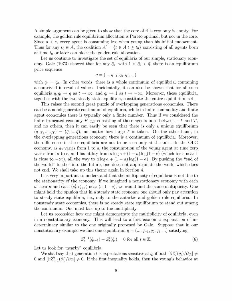
definition of equilibrium is firmly in the Walrasian tradition of agent optimizationand market clearing, we discover three surprises. There are robust examples of OLGeconomies that possess an uncountable multiplicity of equilibria, that are not in thecore, or even Pareto optimal. This lack of optimality (in a slightly different model, aswe shall see) was pointed out by Samuelson in his seminal (1958) paper. The indeter-minacy of equilibrium in the one-commodity case is usually associated first with Gale(1973). In later sections we shall show that these puzzles are robust to an extensionof the model to multiple commodities and agents per period, and to a nonstationaryenvironment. We shall add still another puzzle in Section 3, the positive valuation ofmoney, which is also due to Samuelson.A large part of this section is devoted to developing the notation and price nor-

malization that we shall use throughout. In anyWalrasian model the problem of pricenormalization (the “numeraire problem”) arises. Here the most convenient solutionin the long run is not at first glance the most transparent.Consider an overlapping generation (OLG) economy E = E−∞,∞ in which dis-

crete time periods t extend indefinitely into the past and into the future, t ∈ Z.Corresponding to each time period there is a single, perishable consumption good xt.Suppose furthermore that at each date t one agent is “born’ and lives for two periods,with utility

ut(..., xt, xt+1, ...) = at log xt + (1− at) log xt+1

defined over all vectors

x = (..., x−1, x0, x1, ...) ∈ L = RZ+.

Thus we identify the set of agents A with the time periods Z. Let each agent t ∈ Ahave endowment

et = (..., ett, ett+1, ...) ∈ L

which is positive only during the two periods of his life. Note thatXt∈A

ets = es−1s + ess for all s ∈ Z.

An equilibrium is defined as a (present value) price vector

p = (..., p−1, p0, p1, ...) ∈ L

and allocationx = [xt = (..., xtt, x

tt+1, ...); t ∈ A]

satisfying x is feasible, i.e., Xt∈A

xts =Xt∈A

ets, for all s ∈ Z (1)

5

and Xs∈Z

psets <∞ for all t ∈ A (2)

and

xt ∈ argmaxx∈L

(ut(x)

¯¯Xs∈Z

psxs ≤Xs∈Z

psets

). (3)

The above definition of equilibrium is precisely in the Walrasian tradition, exceptthat it allows for both an infinite number of traders and commodities. All prices arefinite, and consumers treat them as parametric in calculating their budgets. The factthat the definition leads to robust examples with a continuum of Pareto-suboptimalequilibria calls for an explanation. We shall give two of them, one at the end of thissection, and one in Section 4. Note that condition (2) becomes necessary only whenwe consider models in which agents have positive endowments in an infinite numberof time periods.As usual, the set of (present value) equilibrium price sequences displays a trivial

dimension of multiplicity (indeterminacy), since if p is an equilibrium, so is kp forall scalars k > 0. We can remove this ambiguity by choosing a price normalizationqt = pt+1/pt, for all t ∈ Z. The sequence q = (..., q−1, q0, ...) and allocations (xt; t ∈ A)form an equilibrium if (1) above holds together with

xt ∈ argmaxx∈L

{ut(x)|xt + qtxt+1 ≤ ett + qtett+1}. (4)

Notice that we have taken advantage of the finite lifetimes of the agents to combine(2) and (3) into a single condition (4). We could have normalized prices by choosing anumeraire commodity, and setting its price equal to one, say p0 = 1. The normaliza-tion we have chosen instead has three advantages as compared with this more obvioussystem. First, the q system is time invariant. It does not single out a special periodin which a price must be 1; if we relabelled calendar time, then the correspondingrelabelling of the qt would preserve the equilibrium. In the numeraire normalization,after the calendar shift, prices would have to be renormalized to maintain p0 = 1.Second, on account of the monotonicity of preferences, we know that if the preferencesand endowments are uniformly bounded

0 < a ≤ at ≤ a < 1, 0 < e ≤ ett, ett+1 ≤ e ≤ 1 for all t ∈ A,

then we can specify uniform a priori bounds k and k such that any equilibrium pricevector q must satisfy k ≤ qt ≤ k for all t ∈ Z. Thirdly, it is sometimes convenient tonote that each generation’s excess demand depends on its own price. We define

[Ztt(qt), Z

tt+1(qt)] = (x

tt − ett, x

tt+1 − ett+1)

for xt satisfying (4), as the excess demand of generation t, when young and when old.We can accordingly rewrite equilibrium condition (1) as

Zt−1t (qt−1) + Zt

t(qt) = 0 for all t ∈ Z. (5)

6

Let us now investigate the equilibria of the above economy when preferences andendowments are perfectly stationary. To be concrete, let

at = a for all t ∈ A,

and letett = e, and ett+1 = 1− e, for all t ∈ A,

where e > a ≥ 1/2. Agents are born with a larger endowment when young thanwhen old, but the aggregate endowment of the economy is constant at 1 in everytime period. Furthermore, each agent regards consumption when young as at leastas important as consumption when old (a ≥ 1/2), but on account of the skewedendowment, the marginal utility of consumption at the endowment allocation whenyoung is lower than when old:

a

e<1− a

1− e.

If we choose

qt = q =(1− a)e

(1− e)a> 1

for all t ∈ Z, then we see clearly that at these prices each agent will just consume hisendowment; q = (..., q, q, ...) is an equilibrium price vector, with xt = et for all t ∈ A.Note that if we had used the price normalization p0 = 1, the equilibrium prices wouldbe described by

(..., p0, p1, p2, ...) = (..., 1, q, q2, ...)

where pt →∞ as t→∞. With a = 1/2 and e = 3/4, we get q = 3 and pt = 3t.

But there are other equilibria as well. Take q = (..., 1, 1, 1, ...), and

(xtt, xtt+1) = (a, 1− a) for all t ∈ A.

This “golden rule” Pareto equilibrium dominates the autarkic equilibrium previouslycalculated. With a = 1/2 and e = 3/4, we see that (1/2, 1/2) is much better foreveryone than (3/4, 1/4). This raises the most important puzzle of overlapping gen-erations economies: why is it that equilibria can fail to be Pareto optimal? We shalldiscuss this question at length in Section 4.For now, let us observe one more curious fact. We can define the core of our

economy in a manner exactly analogous to the finite commodity and consumer case.We say that a feasible allocation x = (xt; t ∈ A) is in the core of the economy E ifthere is no subset of traders A0 ⊂ A, and an allocation y = (yt; t ∈ A0) for A0 suchthat X

t∈A0yt =

Xt∈A0

et,

andut(yt) > ut(xt) for all t ∈ A0.

7

A simple argument can be given to show that the core of this economy is empty. Forexample, the golden rule equilibrium allocation is Pareto optimal, but not in the core.Since a < e, every agent is consuming less when young than his initial endowment.Thus for any t0 ∈ A, the coalition A0 = {t ∈ A|t ≥ t0} consisting of all agents bornat time t0 or later can block the golden rule allocation.Let us continue to investigate the set of equilibria of our simple, stationary econ-

omy. Gale (1973) showed that for any q0, with 1 < q0 < q, there is an equilibriumprice sequence

q = (..., q−1, q0, q1, ...)

with q0 = q0. In other words, there is a whole continuum of equilibria, containinga nontrivial interval of values. Incidentally, it can also be shown that for all suchequilibria q, qt → q as t → ∞, and qt → 1 as t → −∞. Moreover, these equilibria,together with the two steady state equilibria, constitute the entire equilibrium set.This raises the second great puzzle of overlapping generations economies. There

can be a nondegenerate continuum of equilibria, while in finite commodity and finiteagent economies there is typically only a finite number. Thus if we considered thefinite truncated economy E−T,T consisting of those agents born between −T and T ,and no others, then it can easily be seen that there is only a unique equilibrium(q−T , ..., qT ) = (q, ..., q), no matter how large T is taken. On the other hand, inthe overlapping generations economy, there is a continuum of equilibria. Moreover,the differences in these equilibria are not to be seen only at the tails. In the OLGeconomy, as q0 varies from 1 to q, the consumption of the young agent at time zerovaries from a to e, and his utility from a log e+ (1− a) log(1− e) (which for e near 1is close to −∞), all the way to a log a + (1 − a) log(1 − a). By pushing the “end ofthe world” further into the future, one does not approximate the world which doesnot end. We shall take up this theme again in Section 4.It is very important to understand that the multiplicity of equilibria is not due to

the stationarity of the economy. If we imagined a nonstationary economy with eachat near a and each (ett, e

tt+1) near (e, 1− e), we would find the same multiplicity. One

might hold the opinion that in a steady state economy, one should only pay attentionto steady state equilibria, i.e., only to the autarkic and golden rule equilibria. Innonsteady state economies, there is no steady state equilibrium to stand out amongthe continuum. One must face up to the multiplicity.Let us reconsider how one might demonstrate the multiplicity of equilibria, even

in a nonstationary economy. This will lead to a first economic explanation of in-determinacy similar to the one originally proposed by Gale. Suppose that in ournonstationary example we find one equilibrium q = (..., q−1, q0, q1, ...) satisfying:

Zt−1t (qt−1) + Zt

t(qt) = 0 for all t ∈ Z. (6)

Let us look for “nearby” equilibria.We shall say that generation t is expectations sensitive at qt if both [∂Zt

t(qt)/∂qt] 6=0 and [∂Zt

t+1(qt)/∂qt] 6= 0. If the first inequality holds, then the young’s behavior at

8

time t can be influenced by what they expect to happen at time t+1. Similarly, if thesecond inequality holds, then the behavior of the old agent at time t+ 1 depends onthe price he faced when he was young, at time t. Recalling the logarithmic preferencesof our example, it is easy to calculate that the derivatives of excess demands, for anyqt > 0, satisfy

∂Ztt(qt)

∂qt= atett+1 6= 0

and∂Zt

t+1(qt)

∂qt=−(1− at)ett

q2t6= 0.

Hence by applying the implicit function theorem to (1) we know that there is anontrivial interval IFt−1 containing qt−1 and a function Ft with domain IFt−1 such thatFt(qt−1) = qt, and more generally,

Zt−1t (qt−1) + Zt

t [Ft(qt−1)] = 0 for all qt−1 ∈ IFt−1.

Similarly there is a nontrivial interval IBt containing qt, and a functionBt with domainIBt such that Bt(qt) = qt−1, and more generally, Zt−1

t [Bt(qt)] + Ztt(qt) = 0, for all

qt ∈ IBt . Of course, if Ft(qt−1) = qt ∈ IBt , then Bt(qt) = qt−1.These forward and backward functions Ft and Bt, respectively, hold the key to

one understanding of indeterminacy. Choose any relative price q0 ∈ IF0 ∩ IB0 betweenperiods 0 and 1. The behavior of the generation born at 0 is determined, includingits behavior when old at period 1. If q0 6= q0, and generation 1 continues to expectrelative prices q1 between 1 and 2, then the period 1 market will not clear. However, itwill clear if relative prices q1 adjust so that q1 = F1(q0). Of course, changing relativeprices between period 1 and 2 from q1 to q1 will upset market clearing at time 2, ifgeneration 2 continues to expect q2. But if expectations change to q2 = F2(q1), thenagain the market at time 2 will clear. In general, once we have chosen qt ∈ IFt , we cantake qt+1 = Ft+1(qt) to clear the (t + 1) market. Similarly, we can work backwards.The change in q0 will cause the period 0 market not to clear, unless the previousrelative prices between period −1 and 0 were changed from q−1 to q−1 = B0(q0).More generally, if we have already chosen qt ∈ IBt , we can set qt−1 = Bt(qt) and stillclear the period t market.Thus we see that it is possible that an arbitrary choice of q0 ∈ IF0 ∩ IB0 could lead

to an equilibrium price sequence q. What happens at time 0 is undetermined becauseit depends on expectations concerning period 1, and also the past. But what canrationally be expected to happen at time 1 depends on what in turn is expected tohappen at time 2, etc.There is one essential element missing in the above story. Even if qt ∈ IFt , there

is no guarantee that qt+1 = Ft+1(qt) is an element of IFt+1. Similarly, qt ∈ IBt does notnecessarily imply that qt−1 = Bt(qt) ∈ IBt−1. In our steady state example, this caneasily be remedied. Since all generations are alike,

Ft = F1, Bt = B0, IFt = IF0 and IBt = IB0 for all t ∈ Z.

9

One can show that the interval (1, q) ⊂ IF0 ∩ IB0 , and that if q0 ∈ (1, q), then F1(q0) ∈(1, q), and B0(q0) ∈ (1, q). This establishes the indeterminacy we claimed.In the general case, when there are several commodities and agents per period, and

when the economy is nonstationary, a more elaborate argument is needed. Indeed,one wonders, given one equilibrium q for such an economy, whether after a smallperturbation to the agents there is any equilibrium at all of the perturbed economynear q. We shall take this up in Section 8.It is worth noting that we can define two more complete markets OLG economies

with present value prices. In the economy E0,∞ only agents born at time t ≥ 1participate. The definition of OLG equilibrium is the same as before, except thatnow the set of agents is restricted to the participants, and market clearing is onlyrequired for t ≥ 1. In the q-normalized form, equilibrium is defined by q = (q1, q2, ...)such that

Z11(q1) = 0

Zt−1t (qt−1) + Zt

t(qt) = 0 ∀t ≥ 2

It is immediately apparent (with one agent born per period and one good) that E0,∞has a unique equilibrium, at which no agent trades and which is Pareto inefficient.We could also define an economy EM

0,∞ in which only agents t ≥ 1 participate, butwhere we require (in the normalized price version) that

Z11(q1) = −MZt−1t (qt−1) + Zt

t(qt) = 0 ∀t ≥ 2

Equilibrium in EM0,∞ is as if we gave an outside agent who had no endowment the

purchasing power of M at time 1, and still managed to clear all markets t ≥ 1. Aslong as 0 ≤ M ≤ Z01(q), E

M0,∞ has an equilibrium. Take q0 solving M = Z01(q0), and

q1 = F1(q0) and qt = Ft(qt−1) for t ≥ 2. We examine these two models more closelyin Section 3.

2 Endogenous Cycles

Let us consider another remarkable and suggestive property that one-commodity, sta-tionary OLG economies can exhibit. We shall call the equilibrium q = (..., q−1, q0, q1, ...)periodic of period n if q0, q1, ..., qn−1 are all distinct, and if for all integers i and j,qi = qi+jn. The possibility that a perfectly stationary economy can exhibit cyclicalups and downs, even without any exogenous shocks or uncertainty, is reminiscentof 1930s—1950s business cycle theories. In fact, it is possible to construct a robustone-commodity per period economy which has equilibrium cycles of every order n.Let us see how.As before, let each generation t consist of one agent, with endowment et =

(..., 0, e, 1− e, 0, ...) positive only in period t and t + 1, and utility ut(x) = u1(xt) +

10

u2(xt+1). Again, suppose that q = u02(1 − e)/u01(e) > 1. It is an immediate conse-quence of the separability of ut, that for qt ≤ q,

Ztt(qt) ≤ 0, Zt

t+1(qt) ≥ 0,∂Zt

t+1(qt)

∂qt< 0.

>From monotonicity, we know that Ztt+1(qt) → ∞ as qt → 0. Hence it follows that

for any 0 < q0 < q, there is a unique q−1 = B0(q0) with

Z−10 [B0(q0)] + Z00(q0) = 0.

>From the fact that Z00(q0) ≥ −e for all q0, it also follows that there is some q ≤ 1such that if q0 ∈ [q, q], then B0(q0) ∈ [q, q].Now consider the following theorem due to the Russian mathematician Sarkovsky,

and to the mathematicians Li and Yorke (1975).

Sarkovsky-Li-Yorke Theorem Let B : [q, q] → [q, q] be a continuous functionfrom a nontrivial closed interval into itself. Suppose that there exists a 3-cycle forB, i.e., distinct points q0, q1, q2, in [q, q] with q1 = B(q0), q2 = B(q1), q0 = B(q2).Then there are cycles for B of every order n.

Grandmont (1985), following related work of Benhabib—Day (1982) and Benhabib—Nishimura (1985), gave a robust example of a one-commodity, stationary economy(u1, u2, e) giving rise to a 3-cycle for the function B0. Of course a cycle for B0 is alsoa cyclical equilibrium for the economy, hence there are robust examples of economieswith cycles of all orders.

Theorem (Benhabib, Day, Nishimura, Grandmont) There exist robust examples ofstationary, one-commodity OLG economies with cyclical equilibria of every order n.

This result is extremely suggestive of macroeconomic fluctuations arising for en-dogenous reasons, even in the absence of any fundamental fluctuations. Note, how-ever, that all of the cyclical equilibria, except for the autarkic one-cycle (..., q, q, q, ...)can be shown to be Pareto optimal (see Section 4), while the theory of macroeconomicbusiness cycles is concerned with the welfare losses from cyclical fluctuations. On theother hand, the fact that cyclical behavior is not incompatible with optimality is per-haps an important observation for macroeconomics. More significantly, it must alsobe noted that Sarkovsky’s theorem is a bit of a mathematical curiosity, dependingcrucially on one dimension. And it must also be noted that nonstationary economies,even with one commodity, will typically not have any periodic cycles. By contrast,the multiplicity and suboptimality of nonperiodic equilibria that we saw in Section1 are robust properties that are maintained in OLG economies with multiple com-modities and heterogeneity across time. The main contribution of the endogenousbusiness cycle literature is that it establishes the extremely important, suggestive

11

principle, that very simple dynamic models can have very complicated (“chaotic”)dynamic equilibrium behavior.In the next section we turn to another phenomenon that can generally occur in

overlapping generations economies, but never in finite horizon models.

3 Money and the Sequential Economy

Money very often has value in an overlapping generations model, but it never doesin a finite horizon Arrow—Debreu model. The reason for its absence in the lattermodel is familiar: money would enable some agents to spend more on goods thanthey received from sales of their goods. But that would mean in the aggregate thatspending on goods would exceed revenue from the sale of goods, contradicting marketclearing in goods.This argument can be given another form. Without uncertainty, Arrow—Debreu

equilibrium can be reinterpreted as a sequential equilibrium with contemporaneousprices. But if the number of periods is finite, then in the last period the marginalutility of money to every consumer is zero, hence so is its price. In the second to lastperiod nobody will pay to end up holding any money, because in the last period itwill be worthless. By induction it will have no value even in the first period.Evidently both these arguments fail in an infinite horizon setting. There is no

last period, so the backward induction argument has no place to begin. And with aninfinite number of consumers, aggregate spending and revenue might both be infinite,preventing us from comparing their sizes. On the other hand, there are infinite horizonmodels where money cannot have value. The difference between the OLG model andthese other infinite horizon models will be discussed in Section 7.Strictly speaking, the overlapping generations model we have discussed so far has

been modelled along the lines of Arrow—Debreu: each agent faced only one budgetconstraint and equilibrium was defined as if all markets met simultaneously at thebeginning of time (−∞). In such a model money has no function. However, we candefine another model, similar to the first considered by Samuelson, in which agentsface a sequence of budget constraints and markets meet sequentially, where moneydoes have a store of value role. Surprisingly, this model turns out to have formallythe same properties as the OLG model we have so far considered. To distinguish thetwo models we shall refer to this latter monetary model as the Samuelson model.Suppose that we imagine a one-good per period economy in which the markets

meet sequentially, according to their dates, and not simultaneously at the beginningof time. Suppose also that there are no assets or promises to trade. In such a settingit is easy to see that there could be no trade at all, since, as Samuelson put it, thereis no double coincidence of wants. The old and the young at any date t both have thesame kind of commodity, so they have no mutually advantageous deal to strike. Butas Samuelson pointed out, introducing a durable good called money, which affectsno agent’s utility, might allow for much beneficial trade. The old at date t could

12

sell their money to the young for commodities, who in turn could sell their moneywhen old to the next period’s young. In this manner new and more efficient equilibriamight be created. The “social contrivance of money” is thus connected to both theindeterminacy of equilibrium and the Pareto suboptimality of equilibrium, at leastnear autarkic equilibria. The puzzle, we have said, is how to explain the positiveprice of money when it has no marginal utility.A closer examination of the equilibrium conditions of Samuelson’s sequential mon-

etary equilibrium reveals that although it appears much more complicated, it reducesto the timeless OLG model we have defined above, but with one difference, that thebudget constraint of the generation endowed with money is increased by the valueof money. The introduction of the asset money thus “completes the markets,” inthe sense of Arrow (1953), by which we mean that the equilibrium of the sequentialeconomy can be understood as if it were an economy in which money did not appearand all the markets cleared at the beginning of time (except, as we said, that theincomes of several agents are increased beyond the value of their endowments). Thepuzzle of how money can have positive value in the Samuelson model can thus bereinterpreted in the OLG model as follows. How is it possible that we can increasethe purchasing power of one agent beyond the value of his endowment, without de-creasing the purchasing power of any other agent below his, and yet continue to clearall the markets? Before giving a more formal treatment of the foregoing, let me re-emphasize an important point. It has often been said that the paradoxical propertiesof equilibrium in the sequential Samuelson consumption loan model can be explainedon the basis of incomplete markets. Adding money to the model, however, completesthe markets, in the precise sense of Arrow—Debreu, but the result is the OLG modelin which the puzzles remain.Let us now formally define the sequential one-commodity Samuelson model with

money, EM,S0,∞ . Consider a truncated economy in which there is a new agent “born”

at each date t ≥ 0, whose utility depends only on the two goods dated during hislifetime, and whose endowment is positive only in those same commodities. At eachdate t ≥ 1 there will be two agents alive, a young one and an old one. Let us supposethat trade does not begin until period 1, so that the date 0 generation must consumeits endowment when it is young. To this truncation of our earlier model we now addone extra commodity, which we call money. Money is a perfectly durable commoditythat affects no agent’s utility. Agents are endowed with money (M t

t ,Mtt+1), in addition

to their commodity endowments.A (contemporaneous) price system is defined as a sequence

(π; p) = (π1, π2, ...; p1, p2, ...)

of contemporaneous money prices πt and contemporaneous commodity prices pt for

13

each t ≥ 1. The budget set for any agent t ≥ 1 is defined by©(mt,mt+1, xt, xt+1) ≥ 0|πtmt + ptxt ≤ πtM

tt + pte

tt and

πt+1mt+1 + pt+1xt+1 ≤ πt+1Mtt+1 + pt+1e

tt+1 + πt+1mt

ª.

For agent 0 the budget constraint is©(m0,m1, x0, x1) ≥ 0|m0 =M0

0 , x0 = e00, and

π1m1 + p1x1 ≤ π1M01 + p1e

01 + π1m0

ª.

The budget constraints express the principle that in the Samuelson model agentscannot borrow at all, and cannot save, i.e., purchase more when old than the value oftheir old endowment, except by holding over money mt from when they were young.Let mt

t(π, p) and mtt+1(π, p) be the utility maximizing choices of money holdings by

generation t when young and when old. As before, the excess commodity demand isdefined by Zt

t(π, p) and Ztt+1(π, p).

To keep things simple, we suppose that agent 0 is endowed with M01 = M units

of money when he is old, but all other endowments M ts are zero. Since money is

perfectly durable, total money supply in every period is equal to M . Equilibrium isdefined by a price sequence (π, p) such that for all t ≥ 1,

mt−1t (π, p) +mt

t(π, p) =M and Zt−1t (π, p) + Zt

t(π, p) = 0.

At first glance this seems a much more complicated system than before.But elementary arguments show that in equilibrium either πt = 0 for all t, and

there is no intergenerational trade of commodities, or πt > 0 for all t, or πt < 0 forall t. In the case where πt > 0, no generation will choose to be left with unspent cashwhen it dies, hence mt

t+1(π, p) = 0 for all t, hence money market clearing is reducedto

mtt(π, p) =M for all t ≥ 1.

By homogeneity of the budget sets, if πt > 0, we might as well assume πt = 1 for allt. But then the prices pt become the same as the present value prices from Section1. From period by period Walras Law, we deduce that if the goods market clearsat date t, so must the money market. So we never have to mention money marketclearing or prices.Moreover, by taking qt = (πtpt+1)/(πt+1pt) we can write the commodity excess

demands for agent t ≥ 1 just as in Section 1, by

[Ztt(qt), Z

tt+1(qt)]

and they are the same as[Zt

t(π, p), Ztt+1(π, p)].

14

The only agent who behaves differently is agent 0, whose budget set must now bewritten

B0(μ,M) = {(x0, x1)|x0 = e00, x1 ≤ e01 + μM},where

μ =π1p1.

We can then write agent 0’s excess demand for goods at time 1 as

Z01(μ, q,M) = Z01(μM) = μM

Thus any sequential Samuelson monetary equilibrium can be described by (μ, q),μ ≥ 0, satisfying

Z01(μM) + Z11(q1) = 0,

andZt−1t (qt−1) + Zt

t(qt) = 0 for all t ≥ 2.But of course that is precisely the same as the definition of an OLG equilibrium

for EμM0,∞ given in Section 1.

4 Understanding OLG Economies as Lack ofMarket Clearing at Infinity

In this section we point out that the suboptimality of competitive equilibria, theindeterminacy of nonstationary equilibria, the non-existence of the core, and thepositive valuation of money can all occur robustly in possibly nonstationary OLGeconomies with multiple consumers and L > 1 commodities per period. We also notethe important principle that the potential dimension of indeterminacy is related toL. In the two-way infinity model, it is 2L− 1. In the one-way infinite model withoutmoney it is L− 1; in the one-way infinity model with money the potential dimensionof indeterminacy is L.None of these properties can occur (robustly) in a finite consumer, finite horizon,

Arrow—Debreu model. In what follows we shall suggest that a proper understandingof these phenomena lies in the fact that the OLG model is isomorphic, in a precisesense, to a “∗-finite” model in which not all the markets are required to clear.One of the first explanations offered to account for the differences between the

Arrow—Debreu model and the sequential Samuelson model with money centered onthe finite lifetimes of the agents and the multiple budget constraints each faced. Theseimpediments to intergenerational trade (e.g., the fact that an agent who is “old” attime t logically cannot trade with an agent who will not be “born” until time t+ s)were held responsible. But as we saw in the last section, without uncertainty, thepresence of a single asset like money is enough to connect all the markets. Formally,as we saw, the model is identical to what we called the OLG model in which we could

15

imagine all trade taking place simultaneously at the beginning of time, with eachagent facing a single budget constraint involving all the commodities. What preventstrade between the old and the unborn is not any defect in the market, but a lack ofcompatible desires and resources.Another common explanation for the surprising properties of the OLG model

centers on the “paradoxes” of infinity, as suggested by Shell (1971). In finite models,one proves the generic local uniqueness of equilibrium by counting the number ofunknown prices, less 1 for homogeneity, and the number of market clearing conditions,less 1 for Walras’ Law, and notes that they are equal. In the OLG model there isan infinity of prices and markets, and who is to say that one infinity is greater thananother? We already saw that the backward induction argument against money failsin an infinite horizon setting, where there is no last period. Surely it is right thatinfinity is at the heart of the problem. But this explanation does not go far enough. Inthe model considered by Bewley (1972) there is also an infinite number of time periods(but a finite number of consumers). In that model all equilibria are Pareto optimal,and money never has value, even though there is no last time period. The problem ofinfinity shows that there may be a difference between the Arrow—Debreu model andthe OLG model. In itself, however, it does not predict the qualitative features (likethe potential dimension of indeterminacy) that characterize OLG equilibria.Consider now a general OLG model with many consumers and commodities per

period. We index utilities ut,h by the time of birth t, and the household h ∈ H, afinite set. Household (t, h) owns initial resources et,ht when young, an L-dimensionalvector, and resources et,ht+1 when old, also an L-dimensional vector, and nothing else.As before utility ut,h depends only on commodities dated either at time t or t + 1.Given prices

qt = (qta, qtb) ∈ ∆2L−1++ =

(q ∈ R2L++

¯¯

LX=1

(q + qL+ ) = 2

)consisting of all the 2L prices at date t and t+ 1, each household in generation t hasenough information to calculate the relevant part of its budget set

Bt,h(qt) = {(xt, xt+1) ∈ R2L+ |qta · xt + qtb · xt+1 ≤ qta · et,ht + qtb · et,ht+1}

Hence we can write household excess demand [Zt,ht (qt), Z

t,ht+1(qt)] and the aggregate

excess demand of generation t as [Ztt(qt), Z

tt+1(qt)], where

Ztt+s(qt) =

Xh∈H

Zt,ht+s(qt), s = 0, 1.

Of course we need to put restrictions on the qt to ensure their compatibility, sinceqtb and qt+1,a refer to the same period t+1 prices. But this is easily done by supposingthat

qtb = λtqt+1a for some λt > 0,∀t ∈ Z

16

Present value OLG prices p can always be recovered from the normalized prices qvia the recursion

p1 = q1a

pt = qta(λ1λ2...λt−1) for t ≥ 2pt = qta(λ

−10 λ−1−1...λ

−1t ) for t ≤ 0

We shall now define three variations of the OLGmodel and equilibrium, dependingon when time starts, and whether or not there is money.Suppose first that time goes from −∞ to ∞. We can write the market clearing

condition for equilibrium exactly as we did in the one-commodity, one-consumer case,as

Zt−1t (qt−1) + Zt

t(qt) = 0, t ∈ Z. (A)

Similarly we can define the one-way infinity economy E0,∞, in which time beginsin period 0, but trade begins in time 1. We simply retain the same market clearingconditions for t ≥ 2,

Zt−1t (qt−1) + Zt

t(qt) = 0, t ≥ 2 (A+)Xh∈H

Z0,h1 (q1a) + Z11(q1) = 0 (7)

it being understood that Z0,h1 has been modified to Z0,h1 (q1a) because every agent(0, h) is forced to consume his own endowment at time 0, so that he maximizes overhis budget set

B0,h(q1a) = {(x0, x1) ∈ R2L+ |x0 = e0,h0 , q1a · x1 ≤ q1a · e0,h1 }

Finally, let us define equilibrium in a one-way infinity model with money, EM0,∞,

when agents (0, h) are endowed with money Mh, in addition to their commodities,by (μ, q), μ ≥ 0, satisfyingX

h∈HZ0,h1 (q1a, μM

h) + Z11(q1) = 0, (AM+ )

andZt−1t (qt−1) + Zt

t(qt) = 0, for t ≥ 2.Again it is understood that the agents (0, h) born in time 0 cannot trade in time 0,and they maximize over the budget set

B0,h(q1a, μMh) = {(x0, x1) ∈ R2L+ |x0 = e0,h0 , q1a · x1 ≤ q1a · e0,h1 + μMh}

17

These are the natural generalizations of the one-good economies defined in Section1.1 We must now try to understand very generally why there may be many dimensionsof OLG equilibria, why they might not be Pareto efficient, and how it is possible thatsome agents can spend beyond their budgets without upsetting market clearing.Our explanation amounts to "lack of market clearing at infinitey". We illustrate

this for the case E0,∞.Consider the truncated economy E0,T consisting of all the agents born between

periods 0 and T . Market clearing in E0,T is defined to be identical to that in E0,∞for t = 1 to t = T . But at t = T + 1, we require ZT

T+1(qt) = 0 in E0,T . This is aperfectly conventional Arrow-Debreu economy, and so necessarily has some compet-itive equilibria, all of which are Pareto efficient; generically its equilibrium set is a0-dimensional manifold.We have already seen in Section 1 what a great deal of difference there is between

the economies E0,T (no matter how large T is) and E0,∞. The interesting point isthat by appealing to nonstandard analysis, which makes rigorous the mathematicsof infinite and infinitesimal numbers, one can easily show that the economy E0,T , forT an infinite number, inherits any property that holds for all finite E0,T . Thus theparadoxical properties of the economy E0,∞ do not stem from infinity alone, since theinfinite economy E0,T does not have them. We shall need to modify E0,T before itcorresponds to E0,∞. Nevertheless, the economies E0,T do provide some informationabout E0,∞.

Theorem (Balasko—Cass—Shell and Wilson) Under mild conditions, at least oneequilibrium for E0,∞ always exists.

To see why this is so, note that E0,T is well-defined for any finite T . >From non-standard analysis we know that the sequence E0,T for T ∈ N has a unique extensionto the infinite integers. Now fix T at an infinite integer. We know that E0,T has atleast one equilibrium, since E0,s does for all finite s. But if T is infinite, E0,T includesall the finite markets t = 1, 2, ..., so all those must clear at an equilibrium q∗ of E0,T .Taking the standard parts of the prices q∗t for the finite t (and ignoring the infinite t)gives an equilibrium q for E0,∞.To properly appreciate the force of this proof, we shall consider it again, when it

might fail, in Section 7, where we deal with infinite lived consumers.In terms of the existence of equilibrium, E0,∞ (and similarly EM

0,∞ and E−∞,∞)behaves no differently from an Arrow—Debreu economy. But the indeterminacy is adifferent story.

Definition A classical equilibrium for the economy E0,T is a price sequence q∗ =

1There is one small difference. With many agents born per period we can no longer concludethat if one agent hodls a positive amount of money when young, then so must every other agent (nomatter when he is born). We shall ignore this complication and allow some agents to hold negativemoney.

18

(q1, ..., qT ) that clears the markets for 1 ≤ t ≤ T , but at t = T + 1, market clearingZTT+1(qT ) = 0 is replaced by

ZTT+1(qT ) ≤

Xh∈H

eT+1,hT+1 .

Thus in a classical equilibrium there is lack of market clearing at the last period.The aggregate excess demand in that period, however, must be less than the endow-ment the young of period T + 1 would have had, were they part of the economy.Economies in which market clearing is not required in every market are well under-stood in economic theory. Note that in a classical equilibrium the agents born at timeT are not rationed at T + 1; their full Walrasian (notional) demands are met, out ofthe dispossessed endowment of the young. But we do not worry about how this giftfrom the T +1 young is obtained. The significance of our classical equilibrium for theOLG models can be summarized in the following theorem from Geanakoplos-Brown(1982):

Theorem (Geanakoplos—Brown) Fix T at an infinite integer. The equilibria q forE0,∞ correspond exactly to the standard parts of classical equilibria q∗ of E0,T .

The Walrasian equilibria of the economy E0,∞, which apparently is built on theusual foundations of agent optimization and market clearing, correspond to the “clas-sical equilibria” of another finite-like economy E0,T in which the markets at T + 1(“at infinity”) need not clear. The existence of a classical equilibrium in E0,T , andthus an equilibrium in E0,∞, is not a problem, because market clearing is a specialcase of possible non-market clearing, and E0,T , being finite-like, always has marketclearing equilibria.Thus even though the number of prices and the number of markets in E0,∞ are

both infinite, by looking at E0,T it is possible to say which is bigger, and by how much.There are exactly L more prices than there are markets to clear. From Walras’ Lawwe know that if all the markets but one clear, that must clear as well. Hence having Lmarkets that need not clear provides for L−1 potential dimensions of indeterminacy.

Corollary (Geanakoplos—Brown) For a generic economy E0,∞, there are at mostL− 1 dimensions of indeterminacy in the equilibrium set.

Though the classical equilibria of E0,T generically have L-1 dimensions of inde-terminacy, it is by no means true that there must be L − 1 dimensions of visibleindeterminacy. If we consider any classical equilibrium q∗ for a generic economy E0,T ,then we will be able to arbitrarily perturb some set of L−1 prices near their q∗ values,and then choose the rest of the prices to clear all the markets up through time T . Butwhich L− 1 prices these are depends on which square submatrix N (of derivatives ofexcess demands with respect to prices) is invertible. For example, call the economyE0,∞ intertemporally separable if each generation t consists of a single agent whose

19

utility for consumption at date t is separable from his utility for consumption at datet + 1. Then the L − 1 free parameters must all be chosen at date T + 1 (as part ofqT,b), i.e., way off at infinity.

Corollary (Geanakoplos—Polemarchakis 1984) Intertemporally separable economiesE0,∞ generically have locally unique equilibria (in the product topology).

For example, a natural generalization of the example in Section 1 would be togenerations consisting of a single Cobb-Douglas consumer of L > 1 goods whenyoung and when old. The corollary shows that this economy has no indeterminacyof equilibrium. Since Cobb-Douglas economies seem so central, one might guessthat multi-good OLG economies E0,∞ do not generate indeterminacy. But that isincorrect. Separability with one agent drastically reduces the effect expectationsabout future prices can have on the present, because changes in future consumptiondo not change marginal utilities today. In the separable case changing all L pricestomorrow only affects today through the one dimension of income.Even when the L− 1 degrees of freedom may be chosen at time t = 1, there still

may be no visible indeterminacy, if the matrix N has an inverse (in the nonstandardsense) with infinite norm. But when the free L−1 parameters may be chosen at t = 1and also the matrix N has an inverse with finite norm, then all nearby economiesmust also display L− 1 dimensions of indeterminacy.

Theorem (Kehoe—Levine and Geanakoplos—Brown) In the E0,∞ OLG model thereare robust examples of economies with L − 1 dimensions of indeterminacy. In themonetary economy, EM

0,∞, there are robust examples of economies with L dimensionsof indeterminacy.

Let us now turn our attention to the question of Pareto optimality.

Definition An allocation x = (xt,h; 0 ≤ t ≤ T ) is classically feasible for theeconomy E0,T if

P(t,h)∈A x

t,hs ≤

P(t,h)∈A e

t,hs , for 0 ≤ s ≤ T + 1. The classically

feasible allocation x for E0,T is a classic Pareto optimum if there is no other classicallyfeasible allocation y for E0,T with ut(yt,h) > ut(xt,h) for all (t, h) ∈ A with 0 ≤ t ≤ T ,with at least one inequality (0, h) representing a noninfinitesimal difference.

Theorem (Geanakoplos—Brown) The Pareto-optimal allocations x for the OLGeconomy E0,∞ are precisely the standard parts of classical Pareto-optimal allocationsx∗ for E0,T , if T is fixed at an infinite integer.

The upshot of this theorem is that the effective social endowment includes thecommodities eT+1T+1 of the generation born at time s = T +1, even though they are notpart of the economy E0,T . Since the socially available resources exceed the aggregateof private endowments, it is no longer a surprise that a Walrasian equilibrium, in

20

which the value of aggregate spending every period must equal the value of aggregateprivate endowments, is not Pareto optimal.On the other hand, this does not mean that all equilibria are Pareto suboptimal.

If the (present value) equilibrium prices pt → 0, as t → ∞ (or more generally ifpT+1 is infinitesimal) then the value of the extra social endowment is infinitesimal,and there are no possible noninfinitesimal improvements. To see this, let (p, x) be anequilibrium in present value prices for the OLG economy E0,∞. Consider the concave—convex programming problem of maximizing the utility of agent (0, h), holding allother utilities of agents (t, h) with 0 ≤ t ≤ T at the levels ut,h(xt) they get withx, over all possible allocations in E0,T that do not use more resources, even at timeT + 1, than x. Clearly x itself is a solution to this problem. But now let us imagineraising the constraints at time T + 1 fromX

h∈HxT,hT+1 to

Xh∈H

(eT,hT+1 + eT+1,hT+1 ).

What is the rate of change of the utility u0,h? From standard concave programmingtheorems, for the first infinitesimal additions to period T + 1 resources, the rateof change of u0,h is on the order of pT+1, assuming p1 is normalized to equal themarginal utility of consumption for agent 0, h at date 1. Additional resources bringdecreasing benefits. This shows that if pT+1 is infinitesimal, then there are no possiblenoninfinitesimal improvements with a finite amount of extra resources.An important example of pt → 0 occurs when the prices are summable, as they

are when they decline geometrically to zero. Thus in a stationary equilibrium witha positive real interest rate, equilibrium must be Pareto efficient. Another proof ofefficiency in the case of geometric present value prices is to observe that then thepresent value of the aggregate endowment must be finite, so the standard proof ofPareto efficiency in a finite horizon model goes through.If pt increases geometrically to infinity, then it is evident that equilibrium cannot

be Pareto efficient. Thus in a stationary equilibrium with a negative real interestrate, equilibrium must be Pareto inefficient.When pt 9 0 but also does not increase exponentially to infinity, the calculation

becomes much more delicate. An infinitesimal increase ε in resources at time T+1 canbe used to increase utility of (0, h) on the order of pT+1ε, which is still infinitesimal ifpT+1 is noninfinitesimal but finite. As the increases ε get larger, this rate of changecould drop quickly, as higher derivatives come into play (assuming that agents havestrictly concave utilities), leaving infinitesimal (and thus invisible) increases in utilityeven with a finite increase in resources. Second derivatives, and their uniformity comeinto play. But this subtle case has been brilliantly dealt with:

Theorem (Cass, 1972; Benveniste—Gale, 1975; Balasko—Shell, 1980; Okuno—Zilcha,1981) If agents have uniformly strictly concave utilities, and if the aggregate en-dowment is uniformly bounded away from 0 and ∞, then the equilibrium (p, x) with

21

present value prices p for an OLG economy E0,∞ is Pareto optimal if and only ifP∞t=0 1/||pt|| =∞.

Note that in this theorem it is the present value prices that play the crucialrole. It follows immediately from this theorem that the golden rule equilibrium q =(..., 1, 1, 1, ...) for the simple one good, stationary economy of Section 1 is Paretooptimal, since the corresponding present value price sequence is also (..., 1, 1, 1, ...).In fact, a moment’s reflection shows that any periodic, nonautarkic equilibrium mustalso be periodic in the present value prices p. Hence, as we have said before, butwithout a proof, the cyclical equilibria of Section 2 are all Pareto optimal.Having explained the indeterminacy and Pareto suboptimality of equilibria for

E0,∞ in terms of lack of market clearing at infinity, let us reexamine the monetaryequilibria of OLG economies EM

0,∞, where M = (Mh; h ∈ H) is the stock of moneyholdings by the agents (0, h) at time 0.The next theorem shows that any monetary equilibrium allocation of EM

0,∞ corre-sponds to the standard part of a non-monetary economy E0,T (z) obtained from E0,Tby augmenting the endowments of the first generation (0, h)h∈H by a vector of goodsz at time T + 1.

Definition Let z ∈ RL be a vector of commodities for time T + 1. Suppose that−P

h∈H eT,hT+1 ≤P

h∈H Mhz ≤P

h∈H eT+1,hT+1 . Let the augmented non-monetary econ-omy E0,T (z,M) be identical to the non-monetary economy E0,T , except that theendowment of each agent (0, h) is augmented by Mh · z units of commodities at timeT + 1.

Theorem (Geanakoplos—Brown) Fix an infinite integer T. The equilibria q of themonetary economy EM

0,∞ are precisely obtained by taking standard parts of full marketclearing equilibria q∗ of all the augmented non-monetary economies E0,T (z,M).

The above theorem explains how it is possible to give agents (0, h) extra purchasingpower without disturbing market clearing in the economy EM

0,∞. The answer is thatthe purchasing power comes from owning extra commodities at date T + 1, andequilibrium in EM

0,∞ does not require market clearing in date T + 1 commodities.The above theorem gives another view of why there are potentially L dimensions

of monetary equilibria: the augmenting endowment vector z can be chosen from a setof dimension L. It also explains how money can have positive value: it correspondsto the holding of extra physical commodities. The theorem also explains how the“social contrivance of money” can lead to Pareto-improving equilibria, even in OLGeconomies where there is already perfect financial intermediation. The holding ofmoney can effectively bring more commodities into the aggregate private endowment.The manifestation of the “real money balances” is the physical commodity bundle zat date T + 1. Money plays more than just an intermediation role.Before concluding this section let us consider a simple generalization. Suppose

that agents live for three periods. What plays the analogous role to E0,T? The

22

answer is that prices need to be specified through time T + 2, but markets are onlyrequired to clear through time T . There are therefore 2L − 1 potential dimensionsof indeterminacy, even in the one-sided economy. In general, we must specify theprice vector up until some time s, and then require market clearing only in thosecommodities whose excess demands are fully determined by those prices.This reasoning has an important generalization to production. Suppose that cap-

ital invested at time t can combine with labor at time t+1 to produce output at timet + 1, and suppose that all agents live two periods. Is there any difference betweenthe case where labor is inelastically supplied, and the case where leisure enters theutility? In both cases the number of commodities is the same, but in the latter casethe potential dimension of indeterminacy is one higher, since the supply of labor atany time might depend on further prices.

5 Land, the Real Rate of Interest, and Pareto Ef-ficiency

Allais and Samuelson argued that the infinity of both time periods and agents radi-cally changed the nature of equilibrium. Samuelson suggested that equilibrium mightnot be Pareto efficient, and that the real rate of interest might be negative, even ifthe economy did not shrink over time. In our one-good example from Section 1, theautarkic equilibrium has a negative real interest rate since each qt < 1, and the realinterest rate is 1/qt − 1.They also thought that a second, new kind of equilibrium would emerge in which

the real rate of interest is divorced from any of the considerations like impatience thatIrving Fisher had stressed. They thought that in this new kind of equilibrium the realrate of interest woud turn out to be equal to the rate of population growth, irrespectiveof the impatience of the consumers or the distribution of their endowments. Indeed,in the example from Section 1, the "golden rule" equilibrium had real interest rate1/qt−1 = 0 in every period, irrespective of the utilities or the endowments, but equalto the population growth rate.Furthermore, as we saw in Section 3, Samuelson argued that it might not be

necessary for an asset to be valued according to the present value of its dividends,contradicting yet another one of Fisher’s central concepts. Samuelson suggested thata piece of green paper might be worth a lot, even though it pays no dividends, becausethe holder might think he could sell it to somebody later, who would buy it on theexpectation that he could sell it to somebody else later, ad infinitum. Later authorscalled this a rational bubble.It turns out that these views are incorrect if one includes in the model infinitely

lived assets like land, that do pay dividends in every period.

23

Imagine an OLG economy as before with

ut(xt, xt+1) =1

2log xt +

1

2log xt+1

(ett, ett+1) = (3, 1)

But let us also suppose there is one acre of land in the economy that produces adividend Dt = 1 apple every period forever. Suppose the economy begins in period 1,with an old agent who owns the land and has an endowment of one apple, and a newlyborn agent as above. We suppose that buying the land at time t gives ownership ofall dividends from time t+1 up to and including the dividends in the period in whichthe asset is sold. The apple dividend from the land at time 1 is owned by the oldagent at time 1 (who presumably acquired the land at time 0 and hence has the claimon the apple).At every period t we need to find the contemporaneous price qt of the commodity

and the price Πt of the land.Every agent in the economy must decide how much to consume when young, and

what assets to hold when young, and how much to consume when old. The decisionin old age is trivial, since the agent cannot do better than selling every asset he hasand using the proceeds to buy consumption goods.Thus for every t ≥ 1 we can describe the decision problem of generation t by

maxy,z,θ

ut(y, z) =1

2log y +

1

2log z

such that

qty +Πtθ = qtett = qt3

qt+1z = qt+1ett+1 + θDt+1 +Πt+1θ = qt+11 + θ1 +Πt+1θ

For the original old generation, he optimizes simply by setting

x01 = e01 +D1 +Π1 = 1 + 1 = 2 +Π1

Denote the optimal choice of agents t ≥ 1 by (xtt, xtt+1, θt). Market clearing requiresfor each t ≥ 2 that consumption of the old plus consumption of the young is equal tototal output of goods, and also that demand equals the supply of land

xt−1t + xtt = et−1t + ett +Dt = 1 + 3 + 1 = 5

θt = 1

In period t = 1 we must have

x01 + x11 = e01 + e11 +D1 = 1 + 3 + 1 = 5, θ1 = 1

Sequential equilibrium is thus a vector (x01, (qt,Πt, (xtt, x

tt+1, θ

t))∞t=1) satisfying theabove conditions on agent maximization and market clearing.

24

Fisher’s recipe for computing equilibrium with assets is to put the asset dividendsinto the endowments of their owners, and then find the usual general equilibriumwith present value prices ignoring the assets. In this example that means givingagent 0 an endowment e0 = (2, 1, ...) of two apples in period 1 and one apple everyperiod thereafter, and ignoring the land. Equilibrium with present value prices isthen described exactly as in Section 1.To solve for the present value prices (p1, p2, ...) we can guess that since the economy

is stationary, there will be stationary equilibrium (p1, p2, ...) = (1, p, p2, ...). For each

t ≥ 2, we must solve1

2

[3 + p1]

p+1

2[3 + p1] = 1 + 3 + 1

which gives a quadratic equation

p2 − 6p+ 3 = 0

which is solved by

p =6± (36− 12).5

2= .55, r = 1/p− 1 = 81.7%

The other root is greater than one, and could not be right, because it would give areal interest rate less than zero, which would make the present value of land infinite.Hence consumption when young and old is

(y, z) = (1.775, 3.225)

Clearly these values clear the consumption market for all t ≥ 2. We know by WalrasLaw that if all markets but one clears, then the last will as well, so we don’t reallyhave to check the period 1 market. But we will check it anyway. The present valueof agent 00s endowment is

2 + p1 + p21 + ... = 2 + p/(1− p) = 3.225

and so indeed the period t = 1 market clears.We can now translate this general equilibrium back into a sequential equilibrium.

Taking qt = 1 for every period and the real interest rate solving p = 1/(1 + r), thepresent value of land is

PV Land = p1 + p21 + ... = p/(1− p) =1

1 + r1 +

1

(1 + r)21 + ... = 1.225.

In every period the old will consume their endowment of 1 plus the dividend of 1plus the value of the land they will sell, which gives exactly 3.225. The sequentialequilibrium is (x01, (qt,Πt, (x

tt, x

tt+1, θ

t))∞t=1) = (3.225, (1, 1.225, (1.775, 3.225, 1))∞t=1).

25

Despite what Allais and Samuelson said, the rate of interest at the unique steadystate is positive, higher than the growth rate of population. Moreover, as noted inGeanakoplos (2005), the real interest rate does respond to shocks in exactly the wayFisher argued. Consider the same model as before, but make all the consumers moreimpatient

U(y, z) =2

3log y +

1

3log z

Then our master equation would become

1

3

[3 + p1]

p+2

3[3 + p1] = 1 + 3 + 1

givingp = .419, r = 139%, PV Land = .721

As Fisher would have predicted, the real rate of interest does indeed increase, andthe price of land decreases.

5.1 Pareto efficiency and bubbles

Observe that in our example the dividends of land represent 20% of all endowementsevery period. Since the price of land must be finite, that means in any equilibriumthe present value of all endowments must finite. We know that implies equilibriummust be Pareto efficient.Furthermore, if the value of aggregate endowments is finite, then money cannot

have value and there can be no bubbles, because the old argument is correct thatmarkets cannot clear if some agents are spending more than the value of their com-modity endowments and nobody is spending less. Land makes the OLG economylook much more like an Arrow-Debreu economy.

5.2 Social Security

The overlapping generations model is the workhorse model for examining social se-curity. There is not space here to describe these studies. Observe simply that apay-as-you-go system amounts to a simple transfer of endowments from each youngperson to each old person. We can immediately calculate the effects of such a transferon our steady state interest rate and land value by recomputing the equilibrium forthe OLG economy in which endowments are adjusted to (2, 2) for every generationt ≥ 1, and assuming the old generation 0 has an endowment of 2 apples at time 1plus the land, which pays 1 apple every period. We get

p = .38, r = 161%, PV Land = .62

This also confirms Fisher’s contention that decreasing early endowments and increas-ing later endowments should raise the rate of interest and lower land values.

26

Notice that the pay-go system gives each agent the same number of apples whenhe is old that he gave up when he is young, which is a below market return on hisoriginal contribution. Social security lowers the utility of every agent except the firstgeneration. Samuelson had argued that social security could make every agent betteroff. But his conclusion is false in the model with land.It is often said that if only every generation had more children, social security

would give better returns, since the young would be able to share the burden ofhelping the old. The trouble with that reasoning is that it ignores the fact thathigher population and output growth would mean higher real interest rates, whichtend to make the social security rate of return as bad as before relative to marketinterest rates. There is no space to discuss this here.

6 Demography in OLG

In America over the last 100 years, the generations have alternated in size betweenbig and small. Everybody knows about the baby boom and echo baby boom, butthe same pattern happened before. Recently many authors have suggested that theretiring of the baby boom generation will force stock prices to fall. This has beencriticized on the grounds that demography is easy to predict. If agents knew thatstock prices would fall when the baby boomers retired, they would fall now. Thesetwo opposing views can be analyzed in the OLG model by allowing generation sizesto fluctuate.Suppose the small generation is exactly as before, but now we alternate that small

generation with a large generation that is identical in every respect, except that it istwice as big

ub(y, z) =1

2log y +

1

2log z

(eby, ebz) = (6, 2)

As before suppose that land produces 1 unit of output each period. Begin at time 1with a small generation of young, and suppose the old owns the land.We investigate whether the price of land and the real interest rate alternate be-

tween periods.Let rb be the interest rate that prevails when the big generation b is young, and

ra prevail when the small generation a is young. Equilibrium can be reduced to twoequations. The first describes market clearing for goods in odd periods when thesmall generation is young and the big generation is old, and the second equationdescribes market clearing in even periods, when the big generation is young and the

27

small generation is old. As before, we let pa = 1/(1 + ra) and pb = 1/(1 + rb). Then

1

2

[6 + pb2]

pb+1

2[3 + pa1] = 2 + 3 + 1

1

2

[3 + pa1]

pa+1

2[6 + pb2] = 1 + 6 + 1

These can be simultaneously solved to get

pa = .418, ra = 139%, PVLanda = 1.29

pb = .912, rb = 9.6%, PVLandb = 2.09

It is evident that the price of land is higher in the periods when b is young becausethe interest rate is lower. Even though it is perfectly anticipated that when the biggeneration gets old, the price of land will fall, the price does not fall earlier becausethe interest rate is so low and the land pays dividends.2

7 Impatience and Uniform Impatience

We have already suggested that it is useful in understanding the OLG model toconsider variations, for example in which consumers live forever. By doing so weshall also gain an important perspective on what view of consumers is needed torestore the usual properties of neoclassical equilibrium to an infinite horizon setting,a subject to which we return in Section 8.Let us now allow for consumers t ∈ A who have endowments et that may be

positive in all time periods, and also for arbitrary utilities ut defined on uniformlybounded vectors x ∈ L = RN+. For ease of notation we assume one good per period.A minimal assumption we need about utilities ut is continuity on finite segments,i.e., fixing xs for all s > n, ut(x) should be continuous in (x1, ..., xn). We also needcontinuity on L, in some topology, but we will not go into these details. We alsoassume

Pt∈A e

t is uniformly bounded. In short, we suppose consumers may liveforever.We shall find that in order to have Walrasian equilibria, the consumers must be

impatient. Suppose we try to form the truncated economy E0,T as before, say forT finite. Since utility potentially depends on every commodity, we could not defineexcess demands inE0,T unless we knew all the prices. To make it into a finite economy,let us call E0

0,T the version of E0,T in which every agent is obliged to consume hisinitial endowment during periods t ≤ 0 and t > T . Clearly E0

0,T has an equilibrium.For this to give information about the original economy E0,∞, we need that consumersdo not care very much about what happens to them after T , as T gets very far away.This requires a notion of impatience.

2This point has been made by Geanakoplos, Magill, Quinzii (2004).

28

For any vector x, let nx be the vector which is zero for t > n, and equal tox up until n. Thus nx is the initial n-segment of x. To say that agent t ∈ A isimpatient means that for any two uniformly bounded consumption streams x and y,if ut(x) > ut(y), then for all big enough n, ut(nx) > ut(y). Let us suppose that allconsumers are impatient. If these segments can be taken uniformly across agents,then we say the economy is uniformly impatient. Any finite economy with impatientconsumers is uniformly impatient.Note that the OLG agents are all impatient, since none of them cares about

consumption after he dies, but the economy is not uniformly impatient.Even with an economy consisting of all impatient consumers, the truncation argu-

ment, applied at an infinite E00,T , does not guarantee the existence of an equilibrium.

For once we take standard parts, ignoring the infinitely dated commodities, it mayturn out that the income from the sale of an agent’s endowed commodities at infinitet, which he used to finance his purchase of commodities at finite t, is lost to the agent.It must also be guaranteed that the equilibria of E0

0,T give infinitesimal total value tothe infinitely dated commodities. Wilson (1981) has given an example of an economy,composed entirely of impatient agents, that does not have an equilibrium preciselyfor this reason.On the other hand, if there are only finitely many agents, even if they are infinitely-

lived, then we have:

Theorem (Bewley, 1972) Let the economy E be composed of finitely many, impatientconsumers. Then there exists an equilibrium, and all equilibria are Pareto optimal.

The Pareto efficiency of equilibria in these Bewley economies can be derived fromthe standard proof of efficiency: since there is a finite number of agents, the value ofthe aggregate endowments is a finite sum of finite numbers, and therefore finite itself.In the special case with separable, commonly discounted utilities of the form

uh(x) =P∞

t=0 δtvh(xt), with δ < 1, we have:

Theorem (Kehoe—Levine, 1985) In finite agent, separable commonly discounted util-ity economies, there is generically a finite number of equilibria.

This theorem has been extended by Shannon (1999) and Shannon and Zame(2002).Returning to the case of an infinite number of consumers, Pareto efficiency of

equilibria, if they exist, can be guaranteed as long as a finite number of the agentscollectively hold a non-negligible fraction of total endowment. But that also wouldguarantee the existence of equilibrium, since in the economy E0

0,T we would then getthe summability of the prices, meaning the endowments at infinity would have zerovalue, as Wilson (1981) pointed out.It is extremely interesting to investigate the change in behavior of an economy that

evolves from individually impatient to uniformly impatient. Wilson (1981) considered

29

an example with one infinitely-lived agent, and infinitely many, overlapping, finite-lived agents, and showed that equilibria must exist, and all must be Pareto efficient.By the foregoing remarkes, no matter what the proportion of sizes of the two kinds ofconsumers, equilibria must exist and be Pareto efficient. Muller and Woodford (1988)showed in a particular case that when the single agent’s proportion of the aggregateendowment is low enough, there is a continuum of equilibria, but if it is high enough,there is no local indeterminacy.

8 Comparative Statics for OLG Economies

A celebrated theorem of Debreu assets that almost any Arrow—Debreu economy isregular, in the sense that it has a finite number of equilibria, each of which is locallyunique. Small changes to the underlying structure of the economy (tastes, endow-ments, etc.) produce small, unique changes in each of the equilibria.We have already seen that there are robust OLG economies with a continuum of

equilibria. If attention is focused on one of them, how can one predict to which ofthe continuum of new equilibria the economy will move if there is a small change inthe underlying structure of the economy, perhaps caused by deliberate governmentintervention? In what sense is any one of the new equilibria near the original one?In short, is comparative statics possible?It is helpful at this point to recall that the OLG model is, in spirit, meant to

represent a dynamic economy. Trade may occur as if all the markets cleared simul-taneously at the beginning of time, but the economy is equally well described as iftrade took place sequentially, under perfect foresight or rational expectations. Indeedthis is surely what Samuelson envisaged when he introduced money as an asset intohis model. Accordingly, when a change occurs in the underlying structure of theeconomy, we can interpret it as if it came announced at the beginning of time, or asif it appeared at the date on which it actually affects the economy.We distinguish two kinds of changes to the underlying structure of an economy

E−∞,∞ starting from an equilibrium q. Perfectly anticipated changes, after which wewould look for a new equilibrium that cleared all the markets from the beginning oftime, represent one polar case, directly analogous to the comparative statics exper-iments of the Arrow—Debreu economy. At the other extreme we consider perfectlyunanticipated changes, say at date t = 1. Beginning at the original economy andequilibrium q = (..., q−1, q0, q1, ...), we would look, after the change from E−∞,∞ toE−∞,∞, at time t = 1 (say to the endowment or preferences of the generation bornat time 1), for a price sequence q = (..., q−1, q0, q1, ...) in which qt = qt for t ≤ 0, andZt−1t (qt−1) + Zt

t(qt) = 0 for t ≥ 2. But at date t = 1 we would require q1 to satisfyZ01(q1a|q0) + Z11(q1) = 0, where Z

01(q1a|q0) represents the excess demand of the old at

time 1, given that when they were young they purchased commodities on the strengthof the conviction that they could surely anticipate prices q0b when they got old, onlyto discover prices q1a instead.

30

To study these two kinds of comparative statics, we must describe what we meanby saying that two price sequences are nearby. Our definition is based on the view thata change at time t = 1 ought to have a progressively smaller impact the further awayin time from t = 1 we move. We say that q is near q if the difference |qt− qt| declinesgeometrically to zero, both as t → ∞ and as t → −∞. For perfectly anticipatedchanges, we require that the new equilibrium prices converge geometrically back tothe old prices both as t→∞ and as t→ −∞. For perfectly unanticipated changes,we require that the new equilibrium prices converge geometrically back to the oldprices as t→∞.We have already noted in Section 1 that the multiplicity of OLG equilibria is

due to the fact that at any time t the aggregate behavior of the young generationis influenced by their expectations of future prices, which (under the rational expec-tations hypothesis) depend on the next generation’s expectations, etc. Accordinglywe restrict our attention to generations whose aggregate behavior Zt satisfies theexpectations sensitivity hypothesis:

rank∂Zt

t(pt, pt+1)

∂pt+1= rank

∂Ztt+1(pt, pt+1)

∂pt= L.

For economies composed of such generations we can apply the implicit function the-orem, exactly as in Section 1, around any equilibrium q to deduce the existence ofthe forward and backward functions Ft and Bt. We write their derivatives at q as Dt

and D−1t , respectively.

For finite Arrow—Debreu economies, Debreu gave a definition of regular equilib-rium based on the derivative of excess demand at the equilibrium. He showed thatcomparative statics is sensible at a regular equilibrium, and then he showed that a“generic” economy has regular equilibria. We follow the same program.We say that the equilibrium q for the expectations sensitive OLG economy E is

Lyapunov regular if the long-run geometric mean of the products D∗tDtD

∗t−1Dt−1 · · ·

D∗1D1 and D−1∗

−t D−1−t · · · D−1∗

−1 D−1−1 converge and if to these products we can associate

2L−1 eigenvalues, called Lyapunov exponents. The equilibrium is also nondegenerateif in addition none of these Lyapunov exponents is equal to 1.

Theorem (Geanakoplos—Brown 1985) Let E = E−∞,∞ be an expectations-sensitiveeconomy with a regular nondegenerate equilibrium q. Then for all sufficiently smallperfectly anticipated perturbations E of E (including E itself) E has a unique equi-librium q near q.

Thus the comparative statics of perfectly anticipated changes in the structure ofE, around a regular, nondegenerate equilibrium, is directly analogous to the Arrow-Debreu model. The explanation for the theorem is that a perfectly anticipated changeat time 0 gives rise to price changes that have a forward stable manifold (on whichprices converge exponentially back to where they started) and a backward stable

31

manifold, and that there is only one price at time 0 that is on both the forward andthe backward stable manifolds. Note incidentally that one implication of the abovetheorem is that neutral policy changes, like jawboning or changing animal spirits, i.e.those for which q itself remains an equilibrium, cannot have any effect if they areperfectly anticipated and move the economy to nearby equilibria.

Theorem (Geanakoplos—Brown, 1985) Let E be an expectations-sensitive economywith a regular equilibrium q. Then for all sufficiently small perfectly unanticipatedperturbations E of E (including E itself), the set of unanticipated equilibria q of Enear q is either empty, or a manifold of dimension r, 0 ≤ r ≤ L (L − 1 if there isno money in the economy), where r is independent of the perturbation.

The above theorem allows for the possibility that an unanticipated change mayforce the economy onto a path that diverges from the original equilibrium; the dis-turbance could be propagated and magnified through time. And if there are nearbyequilibria, then there may be many of them. (Indeed that is basically what was shownin Section 4.) In particular, an unanticipated neutral policy change could be com-patible with a continuum of different equilibrium continuations. The content of thetheorem is that if there is a multiplicity of equilibrium continuations, it is parameter-izable. In other words, the same r variables can be held fixed, and for any sufficientlysmall perturbation, there is exactly one nearby equilibrium which also leaves these rvariables fixed. We shall discuss the significance of this in the next section.This last theorem was proved first, in the special case of steady-state economies,

by Kehoe—Levine, in the same excellent paper to which we have referred alreadyseveral times. The theorem quoted here, together with the previous theorem on thecomparative statics of perfectly anticipated policy changes, refers to economies inwhich the generations may be heterogeneous across time.Let us suppose that A is a compact collection of generational characteristics,

all of which obey the expectations-sensitive hypothesis. Let us suppose that eachgeneration’s characteristics are drawn at random from A, according to some Borelprobability measure. If the choices are made independently across time, then theproduct measure describes the selection of economies. Almost any such collectionwill have a complex demographic structure, changing over time. The equilibrium setis then endogenously determined, and will be correspondingly complicated. It can beshown, however that

Theorem (Geanakoplos—Brown, 1985) If the economy E is randomly selected, asdescribed above, then with probability 1, E has at least one Lyapunov regular equilib-rium.

Note that the regularity theory for infinite economies stops short of Arrow—Debreuregularity. In the finite economies, with probability one all the equilibria are regular.

32

9 Keynesian Macroeconomics

Keynesian macroeconomics is based in part on the fundamental idea that changesin expectations, or animal spirits, can affect equilibrium economic activity, includingthe level of output and employment. It asserts, moreover, that publicly announcedgovernment policy also has predictable and significant consequences for economic ac-tivity, and that therefore the government should intervene actively in the marketplaceif investor optimism is not sufficient to maintain full employment.The Keynesian view of the indeterminacy of equilibrium and the efficacy of public

policy has met a long and steady resistance, culminating in the sharpest attack of all,from the so-called new classicals, who have argued that the time-honored microeco-nomic methodological premises of agent optimization and market clearing, consideredtogether with rational expectations, are logically inconsistent with animal spirits andthe non-neutrality of public monetary and bond financed fiscal policy.The foundation of the new classical paradigm is the Walrasian equilibrium model

of Arrow—Debreu, in which it is typically possible to prove that all equilibria arePareto optimal and that the equilibrium set is finite; at least locally, the hypothesis ofmarket clearing fixes the expectations of rational investors. In that model, however,economic activity has a definite beginning and end. Our point of view is that forsome purposes economic activity is better described as a process without end. Ina world without a definite end, there is the possibility that what happens today isunderdetermined, because it depends on what people expect to happen tomorrow,which in turn depends on what people tomorrow expect to happen the day aftertomorrow, etc.Consider the simple one-good per period overlapping generations economy with

money EM,S0 , which we discussed in Section 3. Generation 0 is endowed with money

when young, and equilibrium can be described with the contemporaneous commodityprices p = (p1, p2, ...) where we take the price of money to be fixed at 1.3 It is helpful toreinterpret the model as a simple production economy. Imagine that the endowmentett in the first period of life is actually labor, which can be transformed into output, yt,according to the production function, yt = f( t) = t. We would then interpret anysale of goods by the young generation as real output produced by their labor. Theyoung now derive utility from leisure ett − t in their youth and consumption in theirold age. Equilibrium in which consumption of the old is higher can be interpreted asan equilibrium with less leisure and higher output.The indeterminacy of rational expectations equilibrium thus has the direct inter-

pretation that optimistic expectations by themselves can cause the economy’s outputto expand or contract. In short the economy has an inherent volatility. The Keyne-sian story of animal spirits causing economic growth or decline can be told withoutinvoking irrationality or non-market clearing.

3With the price of money fixed at 1, the contemporaneous prices will be the same as presentvalue prices.

33

In fact, the indeterminacy of equilibrium expectations is especially striking whenseen as a response to public (but unanticipated) policy changes. Suppose the economyis in a long-term rational expectations equilibrium p, when at time 1 the governmentundertakes some expenditures, financed say by printing money. How should rationalagents respond? The environment has been changed, and there is no reason forthem to anticipate that (p2, p3, ...) will still occur in the future. Indeed, in modelswith more than one commodity (such as we will shortly consider) there may be noequilibrium (p1, p2, p3, ...) in the new environment with p2 = p2, p3 = p3, etc. Thereis an ambiguity in what can be rationally anticipated.We argue that it is possible to explain the differences between Keynesian and

monetarist policy predictions by the assumptions each makes about expectationalresponses to policy, and not by the one’s supposed adherence to optimization, marketclearing, and rational expectations, and the other’s supposed denial of all three.Consider now the government policy of printing a small amount of money, ∆M ,

to be spent on its own consumption of real output – or equivalently to be givento generation t = 0 (when old) to spend on its consumption. Imagine first thatagents are convinced that this policy is not inflationary, i.e., that p1 will remain theequilibrium price level during the initial period of the new equilibrium. This will givegeneration t = 0 plus the government consumption level (M +∆M)/p1. As long as∆M is sufficiently small and the initial equilibrium was one of the Pareto-suboptimalequilibria described in Section 1, there is indeed a new equilibrium price path pbeginning with p1 = p1. Output at time 1 rises by ∆M/p1, and in fact this policy isPareto improving. On the other hand, imagine instead that agents are convinced thatthe path of real interest rates pt/pt+1 − 1 will remain unchanged. In this economy,price expectations are a function of p1. Recalling the initial period market-clearingequation, it is clear that now p1 and all future prices rise proportionally to the growth∆M/M in the money stock. The result is output is unchanged and the old at t = 1must pay for the government’s consumption. If the government’s consumption givesno agent utility, the policy is Pareto worsening.This model is only a crude approximation of the differences between Keynesian

and monetarist assumptions about expectations and policy. It is quite possible toargue, for example, that holding p2/p1 = p2/p1 (the future inflation rate) fixed is thenatural Keynesian assumption to make. This ambiguity is unavoidable when there isonly one asset into which the young can place their savings. We are thereby preventedfrom distinguishing between the inflation rate and the interest rate. Our model mustbe enriched before we can perform satisfactory policy analysis. Nevertheless, themodel conveys the general principle that expected price paths are not locally unique.There is consequently no natural assumption to make about how expectations areaffected by policy. A sensible analysis is therefore impossible without externally givenhypotheses about expectations. These can be Keynesian, monetarist, or perhaps somecombination of the two.Geanakoplos—Polemarchakis (1985) builds just such a richer model of macroeco-

34

nomic equilibrium by adding commodities, including a capital good, and a neoclassicalproduction function. With elastically supplied labor, there are two dimensions of in-determinacy. It is therefore possible to fix both the nominal wage, and the firm’sexpectations (“animal spirits”), and still solve for equilibrium as a function of policyperturbations to the economy. These institutional rigidities are more convincinglyKeynesian, and they lead to Keynesian policy predictions. Moreover, taking advan-tage of the simplicity of the two-period lived agents, the analysis can be conductedentirely through the standard Keynesian (Hicksian) IS—LM diagram.Keynesians themselves often postulate that the labor market does not clear. For

Keynesians lack of labor market clearing has at least a threefold significance, which itis perhaps important to sort out. First, since labor is usually taken to be inelasticallysupplied, it makes it possible to conceive of (Keynesian) equilibria with differentlevels of output and employment. Second, it makes the system of demand and supplyunderdetermined, so that endogenous variables like animal spirits (i.e., expectations)which are normally fixed by the equilibrium conditions can be volatile. Third, itcreates unemployment that is involuntary. By replacing lack of labor market clearingat time 1 with elastic labor supply and lack of market clearing “at infinity” onecan drop what seems to many an ad hoc postulate yet retain at least the first twodesiderata of Keynesian analysis.

10 Neoclassical Equilibrium vs. Classical Equilib-rium

The Arrow—Debreu model of general equilibrium, based on agent optimization, ratio-nal expectations, and market clearing, is universally regarded as the central paradigmof the neoclassical approach to economic theory. In the Arrow—Debreu model, con-sumers and producers, acting on the basis of individual self-interest, combine, throughthe aggregate market forces of demand and supply, to determine (at least locally) theequilibrium distribution of income, relative prices, and the rate of growth of capitalstocks (when there are durable goods). The resulting allocations are always Paretooptimal.Classical economists at one time or another have rejected all of the methodolog-

ical principles of the Arrow—Debreu model. They replace individual interest withclass interest, ignore (marginal) utility, especially for waiting, doubt the existence ofmarginal product, and question whether the labor market clears. But by far the mostimportant difference between the two schools of thought is the classical emphasis onthe long-run reproduction of the means of production, in a never-ending cycle.Thus the celebrated classical economist Sraffa writes in Appendix D to his book:

It is of course in Quesnay’s Tableau Economique that is found the orig-inal picture of the system of production and consumption as a circular

35

process, and it stands in striking contrast to the view presented by mod-ern theory, of a one-way avenue that leads from “Factors of Production”to “Consumption Goods.”

The title of his book, Production of Commodities by Means of Commodities, itselfsuggests a world that has no definite beginning, and what is circular can have no end.In the Arrow—Debreu model time has a definite end. As we have seen, that has

strong implications. With universal agreement about when the world will end, therecan be no reproduction of the capital stock. In equilibrium it will be run down tozero. Money, for example, can never have positive value. Rational expectations willfix, at each moment, and for each kind of investment, the expected rate of profit.In the classical system, by contrast, the market does not determine the distribution

of income. Sraffa (1960, p. 33) writes

The rate of profits, as a ratio, has a significance which is independentof any prices, and can well be “given” before the prices are fixed. It isaccordingly susceptible of being determined from outside the system ofproduction, in particular by the money rates of interest. In the followingsections the rate of profits will therefore be treated as the independentvariable.

Other classical writers concentrate instead on the real wage as determined outsidethe market forces of supply and demand, for example, by the level of subsistence orthe struggle between capital and labor. Indeterminacy of equilibrium seems at leastas central to classical economists as it is to Keynesians.Like Keynesians, classicals often achieve indeterminacy in their formal models by

allowing certain markets not to clear in the Walrasian sense. (Again like Keynesians,the labor market is usually among them.) Thus we have called the equilibrium inSection 4 in which some of the markets were allowed not to clear a “classical equilib-rium.”What the OLG model shows is that by incorporating the classical view of the

world without definite beginning or end, it is possible to maintain all the neoclassi-cal methodological premises and yet still leave room for the indeterminacy which isthe hallmark of both classical and Keynesian economics. In particular this can beachieved while maintaining labor market clearing. The explanation for this surpris-ing conclusion is that the OLG model is isomorphic to a finite-like model in whichindeed not all the markets need to clear. But far from being the labor markets, underpressure to move toward equilibrium from the unemployed clamoring for jobs, thesemarkets are off “at infinity,” under no pressure toward equilibrating.We have speculated that once one has agreed to the postulate that the resources of

the economy are potentially as great at any future date as they are today, then uniformimpatience of consumers is the decisive factor, according to Walrasian principles,which may influence whether the market forces of supply and demand determine a

36

locally unique, Pareto-optimal equilibrium, or leave room for extra-market forces tochoose among the continuum of inefficient equilibria. In these terms, the Arrow—Debreu model supposes a short-run impatient economy, and OLG a long-run patienteconomy.

11 Sunspots

So far we have not allowed uncertainty into the OLG model. As a result we foundno difference in interpreting trade sequentially, with each agent facing two budgetconstraints, or “as if” the markets all cleared simultaneously at the beginning of time,with each agent facing one budget constraint. Once uncertainty is introduced theseinterpretations become radically different. In either case, however, there is a vastincrease in the number of commodities, and hence in the potential for indeterminacy.If we do not permit agents to make trades conditional on moves of nature that

occur before they are born, then agents will have different access to asset markets.Even in finite horizon economies, differing access to asset markets has been shown byCass and Shell (1983) to lead to “sunspot effects.”A “sunspot” is a visible move of nature which has no real effect on consumers,

either on account of preferences, or endowments, or through production. In theArrow—Debreu model it also could have no effect on equilibrium trade; this is nolonger true when access to asset markets differs.The sunspot effect is intensified when combined with the indeterminacy that can

already arise in an OLG economy. Consider the simple one good, steady state OLGeconomy of Section 2. Suppose that there is an equilibrium two cycle in presentvalue prices p = (..., p−1, p0, p1, ...) with p2t = pS and p2t+1 = pR, for all t ∈ T . Nowsuppose that the sun is known to shine on even periods, and hide behind rain on oddperiods. The above equilibrium is perfectly correlated with the sun, even though noagent’s preferences or endowments are. As usual, the same prices for t ≥ 0 supportan equilibrium, given the right amount of money, in EM,S

0,∞ .More generally, suppose that the probability of rain or shine, given the previous

period’s weather, is given by the Markov matrix π = (πSS, πSR, πRS, πRR). A steadystate equilibrium for EM,S

0,∞ , given π, is an assignment of a money price for the com-modity, depending only on that period’s weather, such that if all agents maximizetheir expected utility with respect to π, then in each period the commodity marketand money market clears. Azariadis (1981) essentially showed that if there is a two-cycle of the certainty economy, then there is a continuum of steady state sunspotequilibria.The sunspot equilibria, unlike the cyclical equilibria of Section 2, are Pareto sub-

optimal whenever the matrix π is nondegenerate.The combination of the dynamic effects of the infinite horizon OLG model with

the burgeoning theory of incomplete markets under real uncertainty, is already onthe agenda for next generation’s research.

37

12 Bibliography

Allais, M. 1947. Economie et interêt. Paris: Imprimerie, Nationale.

Arrow, K. J., 1953. “The Role of Securities in the Optimal Allocation of Risk-Bearing.” Reprinted in K. J. Arrow, Essays in the theory of Risk Bearing.Chicago: Markham, 1971.

Azariadis, C. 1981. “Self-fulfilling Prophecies,” Journal of Economic Theory 25(3):380—396.

Balasko, Y., and K. Shell. 1980. "The Overlapping-Generations Model, I: TheCase of Pure Exchange without Money," Journal of Economic Theory 23(3):281-306.

Balasko, Y., D. Cass, and K. Shell. 1980. “Existence of Competitive Equilibriumin a General Overlapping-Generations Model,” Journal of Economic Theory23(3): 307—322.

Benhabib, J. and R. H. Day. 1982. “A Characterization of Erratic Dynamics in theOverlapping Generations Model,” Journal of Economic Dynamics and Control4: 37—44.

Benhabib, J., and N. Nishimura, 1985. “Competitive Equilibrium Cycles,” Journalof Economic Theory (35): 284—306.

Benveniste, L. and D. Gale. 1975. “An Extension of Cass’ Characterization ofInfinite Efficient Production Programs,” Journal of Economic Theory 10: 229—238.

Bewley, T. 1972. “Existence of Equilibria in Economies with Infinitely Many Com-modities,” Journal of Economic Theory 4: 514—540.

Cass, D. 1972. “On Capital Overaccumulation in the Aggregative, NonclassicalModel of Economic Growth,” Journal of Economic Theory, 4(2): 200—223.

Cass, D. and K. Shell. 1983. "Do Sunspots Matter?" Journal of Political Economy,91, 193-227.

Cass, D. and M. E. Yaari. 1966. “A Re-examination of the Pure Consumption LoanModel,” Journal of Political Economy, 74(2): 200—223.

Debreu, G. 1970. “Economies with a Finite Set of Equilibria,” Econometrica 38:387—392.

Diamond, P. A. 1965. “National Debt in a Neo-classical Growth Model,” AmericanEconomic Review, 55(5): 1126—1150.

38

Fisher, I. 1907. The Rate of Interest. New York. MacMillan.

Fisher, I. 1930. The Theory of Interest. New York. MacMillan.

Gale, D. 1973. “Pure Exchange Equilibrium of Dynamic Economic Models,” Journalof Economic Theory, 6(1): 12—36.

Geanakoplos, J., 1978, 1980. “Sraffa’s Production of Commodities by Means of Com-modities: Indeterminacy and Suboptimality in Neoclassical Economics. RIASWorking Paper (1978), also Ch. 3 of “Four Essays on the Model of Arrow—Debreu,” Ph.D Dissertation, Harvard University (1980).

Geanakoplos, J. 2005. "The ideal inflation indexed bond and Irving Fisher’s Theoryof Interest with Overlapping Generations," in Celebrating Irving Fisher: TheLegacy of a Great Economist (R. Dimand and J. Geanakoplos eds) Journal ofEconomics and Sociology, vol 64, 1, 257-305, Blackwell Publishing, Oxford.

Geanakoplos, J. and D. Brown. 1982. “Understanding Overlapping GenerationsEconomies as Lack of Market Clearing at Infinity,” Yale University, mimeo,revised 1985, 1986.

Geanakoplos, J. and D. Brown. 1985. “Comparative Statics and Local Indetermi-nacy in OLG Economies: An Application of the Multiplicative Ergodic Theo-rem,” Cowles Foundation Discussion Paper No. 773.

Geanakoplos, J. and H. M. Polemarchakis. 1984. “Intertemporally Separable Over-lapping Generations Economies,” Journal of Economic Theory 34: 207—215.

Geanakoplos, J., and H. M. Polemarchakis, 1985. “Walrasian Indeterminacy andKeynesian Macroeconomics,” Review of Economic Studies, 53(5): 755—799.

Geanakoplos, J., Michael Magill, and Martine Quinzi, 2004. “Demography and theLong-Run Predictability of the Stock Market,” Brookings Papers on EconomicActivity, 1: 241—325

Grandmont, J. M. 1985. “Endogenous, Competitive Business Cycles,” Economet-rica, 53(5): 995—1046.

Kehoe, T. J. and D. K. Levine. 1984. “Regularity in Overlapping GenerationsExchange Economies,” Journal of Mathematical Economics 13: 69—93.

Kehoe, T. J. and D. K. Levine. 1985. “Comparative Statics and Perfect Foresightin Infinite Horizon Models,” Econometrica 53: 433—453.

Kehoe, T. J., D. K. Levine, and P. M. Romer. 1990. “Determinacy of Equilibria inDynamic Models with Finitely Many Consumers,” Journal of Economic Theory50, 1-21.

39

Keynes, J. M. 1936. The General Theory of Employment, Interest and Money.London: Macmillan.

Li, T. Y., and J. A. Yorke, 1975. “Period Three Implies Chaos,” The AmericanMathematical Monthly. 8(10): 985—992.

Lucas, R. E. 1972. “Expectations and the Neutrality of Money,” Journal of Eco-nomic Theory 4(2): 102—121.

Muller, W. J. and M. Woodford. 1983. “Determinacy of Equilibrium in StationaryEconomies with both Finite and Infinite Lived Consumers,” Journal of Eco-nomic Theory, 46, 255-290.

Okuno, M. and I. Zilcha. 1980. "On the Efficiency of a Competitive Equilibriumin Infinite Horizon Monetary Economies," Review of Economic Studies XLVII,797-807.

Samuelson, P. A. 1958. “An Exact Consumption Loan Model of Interest, With orWithout the Social Contrivance of Money,” Journal of Political Economy 66(5):467—482.

Shannon, C. 1999. "Determinacy of Competitive Equilibria in Economies with ManyCommodities" Economic Theory, 14(1), 29-87.

Shannon, C, and B. Zame. 2002. "Quadratic Concavity and Determinacy of Equi-librium", Econometrica, 70(2), 631-662.

Shell, K. 1971. “Notes on the Economics of Infinity,” Journal of Political Economy,79, 1002—1011.

Sraffa, P. 1960. Production of Commodities by Means of Commodities. Cambridge:Cambridge University Press.

Wilson, C. 1981. “Equilibrium in Dynamic Models with an Infinity of Agents,”Journal of Economic Theory 24(1): 95—111.

40