Fertility and mortality changes in an overlapping-generations model with realistic demography

Sau-Him Paul Lau *

University of Hong Kong

March 2009

Abstract Many overlapping-generations models only assume working and retirement stages and are “not capable of representing the most basic feature of the human economic life cycle: that it begins and ends with periods of dependency, separated by a long intermediate period of consuming less than is produced” (Bommier and Lee, 2003). To examine the economic consequences of fertility and mortality changes, we incorporate more realistic demographic features in an overlapping-generations model. In particular, we include a childhood stage, link the mortality changes to changes in life expectancy, and relate fertility changes to changes in the total fertility rate (which is independent of the age composition of the population). We use the model to study the impact of demographic changes on capital accumulation. Interestingly, we find that an increase in fertility and a reduction in mortality, while both causing a rise in the population growth rate, lead to opposite effects on capital accumulation. To provide intuition of these results, we decompose the impact of a demographic change into capital dilution and aggregate saving effects. For an endogenous change in aggregate saving, we further decompose it into individual saving and age-structure effects. JEL Classification Numbers: J10; E21 Keywords: overlapping generations, age-specific mortality, childhood years, retirement Correspondence: S.-H. P. Lau, School of Economics and Finance, University of Hong Kong, Pokfulam, Hong Kong Phone: (852) 2857 8509 Fax: (852) 2548 1152 E-mail: laushp@hkucc.hku.hk * I am grateful to Chad Jones, Andrew Mason, Miguel Sanchez-Romero, seminar participants at UC Berkeley and especially Ron Lee for helpful comments and suggestions, and to Tsz Kin Chan for research assistance. This project was initiated during a visit at the Center on the Economics and Demography of Aging, UC Berkeley. Their hospitality is gratefully acknowledged. I also thank the Research Grants Council of Hong Kong (through GRF project HKU7463/08H) and the Fulbright Visiting Scholar Program for generous financial support.

1. INTRODUCTION

Researchers and policy makers have long been interested in the relationship of

demographic changes, capital accumulation and economic growth (Ehrlich and Lui,

1997). In the more formal approach of modern-day economics, the Solow (1956) model

predicts that an exogenous increase in the population growth rate decreases steady-

state output per worker (or output per unit of effective labor if there is technological

progress) through the capital dilution effect. On the other hand, this exogenous

change has no effect on output per worker in the Ramsey-Cass-Koopmans model

(Ramsey, 1928; Cass, 1965; Koopmans, 1965), since optimizing individuals respond

by decreasing consumption and increasing saving.

While the Ramsey-Cass-Koopmans model with infinitely-lived individuals or dy-

nasties can be used to examine the economic consequences and welfare implications

of demographic changes, the overlapping-generations (OLG) model is, arguably, a

better framework to use. The finite life of mortal individuals is most naturally mod-

elled in such a framework, and the interaction of different cohorts’ decisions can be

meaningfully studied. However, in two most well-known OLG models (Diamond’s

(1965) two-period model and Blanchard’s (1985) continuous-time model with age-

invariant mortality rates), the demographic assumptions are made in a tractable but

not-so-realistic manner, in order to focus on other economic factors. Thus, while

these models are useful to analyze issues such as the impact of social security or gov-

ernment debt policies, they are less suited to analyze the economic consequences of

demographic changes.1 In particular, uncertainty in lifetime is not modelled in Dia-

mond (1965), and people are assumed to live two periods and then die. In Blanchard

(1985), lifetime uncertainty is modelled, but the assumption of age-invariant mor-1As demographic (and related labor supply) pattern has been changing quite significantly in many

industrial countries, a lot of researchers are interested in the economic effects of these changes. See,

for example, Cutler et al. (1990) and Boucekkine et al. (2002).

2

tality is quite different from the human experience. The types of mortality changes

observed in industrial countries in recent years cannot be meaningfully analyzed in

these models.

To allow for a more general demographic structure, some recent articles (such as

Boucekkine et al., 2002; Bommier and Lee, 2003; Faruqee, 2003; Echevarria and

Iza, 2006; d’Albis, 2007; Lau, 2009) consider OLG models with lifetime uncertainty

captured by age-specific mortality rates.2 For the parametric approach to model the

human survival function, Boucekkine et al. (2002) and Echevarria and Iza (2006) use

a form based on the exponential function and Faruqee (2003) works with a hyperbolic

tangent function. On the other hand, Bommier and Lee (2003), d’Albis (2007) and

Lau (2009) assume a general mortality pattern. In particular, d’Albis (2007) uses a

general age-specific mortality schedule in an OLG model with neoclassical production

function, and shows that the effect of a fertility increase on capital accumulation

can be positive or negative, in sharp contrast with the negative relation predicted in

Diamond (1965) and Blanchard (1985). Lau (2009) provides a quantitative assessment

of these theoretical predictions, and finds that while the ambiguous effects predicted

by d’Albis (2007) are possible, in practice the effects of fertility increases on capital

accumulation are negative for industrial countries.

There are two objectives in this paper. First, it extends the analysis of fertility

changes in d’Albis (2007) and Lau (2009) to include mortality changes as well. It

is obvious that even in an economy closed to immigration, population changes can

be caused by either fertility or mortality factors. On an empirical level, fertility

reduction in industrial countries has been very substantial in the last two countries,2Earlier work include Arthur and McNicoll (1977, 1978). Note that we mainly refer to papers

using continuous-time overlapping-generations models since we focus on this type of models in this

paper. There is also a large literature on discrete-time overlapping-generations models with general

demographic structure. A leading example is Auerbach and Kotlikoff (1987).

3

and future fertility changes are likely to be less drastic. On the other hand, mortality

changes in these countries continue to happen, especially for the old and the oldest old.

Thus, when considering the economic impact of demographic changes (say, on capital

accumulation), it is at least equally important to consider the effect of mortality

changes. One objective of this paper is to study the effect of mortality changes on

capital accumulation. Interestingly, we find that a rise in fertility and a reduction

in mortality, while both causing an increase in the population growth rate, lead to

opposite effects on capital accumulation. After presenting these results in Sections

4 and 5, we use a standard framework in growth analysis to provide intuition of the

results.

Our second objective is to present a model with more realistic demographic features

to analyze fertility and mortality changes. Many OLG models–including discrete-

time models such as Diamond (1965) and Abel (2003), and continuous-time models

such as Blanchard (1985), d’Albis (2007), and Lau (2009)–only assume one stage

(working) or two stages (working and retirement) of the life cycle. As mentioned

in Bommier and Lee (2003, p. 136), “Two age group models are not capable of

representing the most basic feature of the human economic life cycle: that it begins

and ends with periods of dependency, separated by a long intermediate period of

consuming less than is produced.” In studying the consequences of demographic

changes, an OLG model consisting of childhood, working and retirement stages is

more appropriate than a two-stage model. A more accurate modelling of the human

economic life cycle is particularly important, if we want to consider the quantitative

implications.

This paper contributes to the methodological aspects of continuous-time OLGmod-

els with childhood, working and retirement stages in several aspects. First, we link

mortality changes based on changes in life expectancy at birth, a concept familiar

to most social scientists. To overcome the problem that the relationship between

4

mortality changes and changes in life expectancy is not one-to-one in general, we use

the method based on Lee and Carter (1992) to achieve a one-to-one correspondence

between changes in life expectancy and the empirical changes in mortality pattern.

Second, instead of relating fertility changes to changes in the crude birth rate, which

is commonly used in the literature, we relate fertility changes to changes in the total

fertility rate (TFR), and conduct the analysis based on actual TFR rate data. The

TFR is defined as the average number of children who would be born per woman dur-

ing her reproductive years, if she survives to the end of her reproductive years. Thus,

while the crude birth rate confounds behavioral and age-structure effects, the TFR

has the advantage of not being affected by the age composition of the population.

Third, we show that the equilibrium of the two-stage OLG model used in d’Albis

(2007) and Lau (2009) arises as a special case of the equilibrium of the three-stage

OLG model developed in this paper, when a parameter determining the number of

effective adult consumers in the household tends to zero.

The paper is organized as follows. In Section 2 we first describe an OLG model

with realistic demography by incorporating relevant features of age-specific mortality

rates, childhood years and retirement years. To facilitate comparison with existing

models and to balance between realism and tractability, the demographic aspects of

the model are relatively complicated while the economic aspects are kept simple and

standard. In Section 3 we characterize the steady-state equilibrium of the model,

and examine its existence and uniqueness. We also relate the model in this paper to

d’Albis (2007) and Lau (2009). We study quantitatively the economic consequences

of fertility and mortality changes in this model in Sections 4 and 5, respectively. In

Section 6 we provide intuitions of the results. Section 7 concludes.

5

2. THE MODEL

The continuous-time OLG model used in this paper is modified from Blanchard

(1985), which incorporates important features from Yaari (1965). Irrespective of the

age of an individual, the exposure risk to mortality is assumed to be constant in

Blanchard (1985). With this assumption (and the presence of actuarially-fair an-

nuity contracts), individuals of different ages have the same marginal propensity to

consume, despite their different wealth levels. The constancy of the marginal propen-

sity to consume for different individuals allows aggregation to be done in a relatively

easy manner. Another demographic assumption made in Blanchard (1985) is that

the birth and death rates are the same so that the population size is constant (in

an economy without immigration). Under these two assumptions, the age distribu-

tion of the population is time-invariant. This is known as a stationary population,

which is a special case of a stable population in the demographic literature. Lotka

(1939) shows that when age-specific fertility and mortality rates are time-invariant,

the population will eventually grow at a constant rate and the proportion in each age

group is unchanged over time. (See Coale (1972) and Keyfitz and Caswell (2005), for

example, for more detailed discussion about stable population.)

The assumption of constant population size can easily be relaxed. Weil (1989)

assumes no death rate and a positive birth rate in the Blanchard (1985) model. Al-

lowing the features in Blanchard (1985) and an early version of Weil (1989), Buiter

(1988) assumes that the birth and death rates are non-negative and may be differ-

ent. On the other hand, it is well known that when the assumption of age-invariant

mortality rates is relaxed, analytical aggregation formula is in general not available.

Nevertheless, using the idea of the stable population theory, it is possible to obtain

useful relationships among aggregate economic variables in the steady-state equilib-

rium, even when mortality rates are not age-invariant (see Bommier and Lee, 2003;

6

d’Albis, 2007; Lau, 2009).

In this paper we depart from the assumption of age-invariant mortality in Blanchard

(1985) and use the actual life table data. Define the probability that an individual

survives to at least age x as the survival function l (x), where x ∈ [0,Ω] , Ω is the

maximum possible age of an individual (l (Ω) = 0), and l (0) is normalized to 1. The

most recent survival function based on the population (men and women combined) of

USA in 2005, which is obtained from the Human Mortality Database (HMD, 2008),

is shown in Figure 1. The instantaneous mortality rate at age x, μ (x), is related to

the decreasing function l (x) by

μ (x) = − 1

l (x)

dl (x)

dx. (1)

The mortality rates (in natural log) at different ages for USA in 2005 are shown in

Figure 2. It is clear that they are hugely inconsistent with the age-invariant mortality

assumption.

In this paper, we incorporate age-specific mortality rates and other demographic

features in an OLG model to study fertility and mortality changes. In general, at

least three types of activities–consumption over time, fertility, and retirement–

should be examined in studying the economic consequences of demographic changes.

The modelling of these decisions can easily become intractable. Several features of the

OLGmodel used in this paper are chosen to balance the tractability consideration and

a reasonably accurate description of the economic and demographic characteristics of

industrial countries.3

3This paper focuses on industrial countries (such as USA) where demographic transition has

progressed to a large extent. Demographic transition refers to the process during which a country

moves “from a state of low and fairly stagnant per capita income, high mortality, and high fertility to

a regime of persistent growth in which first mortality, and then fertility are continuously declining ...”

(Ehrlich and Lui, 1997, p. 224). The economic consequences of demographic changes in developing

countries which are in an early stage of demographic transition are likely to be quite different from

7

First, the average growth rate of output per worker is roughly constant over a long

period of time in industrial countries (Jones, 1995), despite a substantial change in

demographic variables. Thus, we consider a neoclassical production function with

constant rate of exogenous technological progress. Second, average retirement age

in industrial countries remains roughly unchanged (or even experiences a mild drop)

in the last fifty years, despite the significant improvement in longevity. We do not

investigate the reasons of this phenomenon in this paper, but simply take retirement

age to be exogenously fixed. Third, we follow Boucekkine et al. (2002) and d’Albis

(2007) to assume that aggregate output is endogenous, but fertility and mortality

changes are exogenous. While the assumption that changes in aggregate output (or,

more generally, in level of development) and mortality changes do not affect fertility

decisions may not be appropriate for countries in the early stage of demographic

transition, they seem to be more reasonable for industrial countries which are at a

more advanced stage of demographic transition.

The time line of a cohort s individual’s various activities (up to the maximum

possible age Ω), in a stylized fashion, is given in Figure 3. From the time of birth (at

time s) to age Tw (at time s + Tw), an individual is in the childhood stage and does

not have to make economic decisions. The levels of consumption during these years

are determined by her parent.4 An individual becomes an adult at age Tw and works

from that age until retirement at age Tr. She also makes consumption decisions (and,

implicitly, saving and capital accumulation decisions) from age Tw until the end of her

life (which is at most Ω). Regarding the parental role, it is assumed that she will give

those of industrial countries, and will not be examined in this paper. (See the last paragraph of the

Conclusion for a suggested model more appropriate in studying the impact of demographic changes

in developing countries.)4Consumption is the only decision in the childhood stage since other potentially important factors

(such as human capital accumulation) are not modelled. Note also that, for simplicity, we use a

one-parent model in this paper.

8

rise to (possibly fractional) β babies at age Tb if she survives to that age,5 and she

is responsible for the children’s consumption from birth to age Tw (corresponding to

the parent’s age from Tb to Tb+Tw) as well. In the quantitative exercises, we assume

Ω = 110, Tr = 65, Tb = 28 and Tw = 20, based on stylized facts of many developed

countries.

Parameter β is related to the demographic concept of TFR as follows. With the

commonly-used assumption that the male to female ratio at birth is 1.05 (which is

also the sex ratio at birth of USA in 2005), we have

β =TFR

2.05. (2)

Denote B (t) as the number of births at time t. Based on the fertility and mortality

descriptions above, it is given by

B (t) = B (t− Tb) l (Tb)β. (3)

Since age-specific mortality and fertility rates are time-invariant in this economy, the

population is stable (Lotka, 1939). Let n be the constant growth rate of the number

of births (such that B (t) = B (0) ent). It can be shown from (2) and (3) that n is

given by:

n =1

Tblog

∙l (Tb)TFR

2.05

¸. (4)

Based on the birth and death histories of different cohorts, the population at time

t is obtained by aggregating surviving individuals of different ages as follows:

P (t) =

Z t

t−ΩB (s) l (t− s) ds =

Z t

t−ΩB (t) e−n(t−s)l (t− s) ds = B (t)

Z Ω

0

e−nxl (x) dx.

(5)

Since the termR Ω

0e−nxl (x) dx in (5) is independent of time t, we conclude that the

population grows at the same rate as that of the number of birth.5Note that the assumption that all births occur at age Tb is the simplest way to represent age-

specific fertility rates. We use the mean age of childbearing to choose Tb.

9

Labor supply at any age is assumed to be exogenous and either zero or full time

(which is normalized to 1) in this paper. Therefore, its level is given by

N (s, s+ x) =

⎧⎨⎩ 1 if Tw ≤ x ≤ Tr0 otherwise

, (6)

where N (s, v) is the labor supply of a cohort s individual at time v. Similar to (5),

aggregate labor supply N (t) is given by

N (t) =

Z t

t−ΩB (s) l (t− s)N (s, t) ds = B (t)

Z Tr

Tw

e−nxl (x) dx, (7)

and it grows at the same rate (i.e., n) as the population.

Except for the age-specific mortality rates, the presence of childhood years and the

specification of labor supply during working and retirement years, the other aspects

of the Blanchard (1985) model are retained in the following analysis. Specifically, it is

assumed that an individual begins her adult life without financial assets or liabilities,

and she cannot leave any debt at her death. As a result,

Z (s, s+ Tw) = 0; Z (s, s+ Ω) ≥ 0, (8)

where Z (s, v) is the financial wealth of a cohort s individual at time v.

We now examine an individual’s consumption decision. To focus purely on the

saving-for-retirement motive, we follow Blanchard (1985) and d’Albis (2007) to as-

sume that individuals have no bequest motive. An individual born at time s chooses

C (s, v)s+Ωt , at time t (where s + Tw ≤ t ≤ s+ Ω), to maximizeZ s+Ω

t

e−ρ(v−t)l (v − s)l (t− s) λ (v − s)

"C (s, v)1−

1σ − 1

1− 1σ

#dv, (9)

subject to the flow budget constraint

∂Z (s, v)

∂v= [r (v) + μ (v − s)]Z (s, v) + w (v)N (s, v)− C (s, v)λ (v − s) , (10)

10

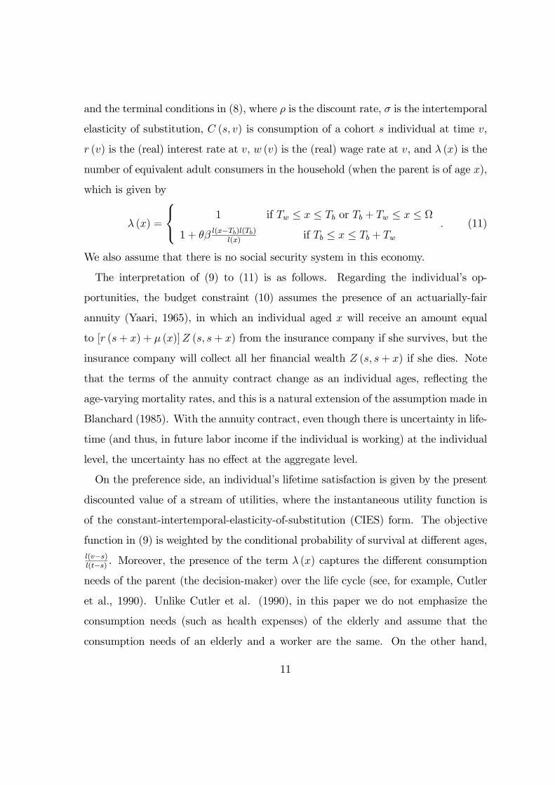
and the terminal conditions in (8), where ρ is the discount rate, σ is the intertemporal

elasticity of substitution, C (s, v) is consumption of a cohort s individual at time v,

r (v) is the (real) interest rate at v, w (v) is the (real) wage rate at v, and λ (x) is the

number of equivalent adult consumers in the household (when the parent is of age x),

which is given by

λ (x) =

⎧⎨⎩ 1 if Tw ≤ x ≤ Tb or Tb + Tw ≤ x ≤ Ω

1 + θβ l(x−Tb)l(Tb)l(x)

if Tb ≤ x ≤ Tb + Tw. (11)

We also assume that there is no social security system in this economy.

The interpretation of (9) to (11) is as follows. Regarding the individual’s op-

portunities, the budget constraint (10) assumes the presence of an actuarially-fair

annuity (Yaari, 1965), in which an individual aged x will receive an amount equal

to [r (s+ x) + μ (x)]Z (s, s+ x) from the insurance company if she survives, but the

insurance company will collect all her financial wealth Z (s, s+ x) if she dies. Note

that the terms of the annuity contract change as an individual ages, reflecting the

age-varying mortality rates, and this is a natural extension of the assumption made in

Blanchard (1985). With the annuity contract, even though there is uncertainty in life-

time (and thus, in future labor income if the individual is working) at the individual

level, the uncertainty has no effect at the aggregate level.

On the preference side, an individual’s lifetime satisfaction is given by the present

discounted value of a stream of utilities, where the instantaneous utility function is

of the constant-intertemporal-elasticity-of-substitution (CIES) form. The objective

function in (9) is weighted by the conditional probability of survival at different ages,l(v−s)l(t−s) . Moreover, the presence of the term λ (x) captures the different consumption

needs of the parent (the decision-maker) over the life cycle (see, for example, Cutler

et al., 1990). Unlike Cutler et al. (1990), in this paper we do not emphasize the

consumption needs (such as health expenses) of the elderly and assume that the

consumption needs of an elderly and a worker are the same. On the other hand,

11

we emphasize the well-known fact that the consumption needs of children are less

than those of adults (i.e., θ < 1). In one of the definition (CONS) used in Cutler et

al. (1990), they assume that children’s consumption needs equal to one-half those of

adults (θ = 0.5). The relatively unfamiliar term l(x−Tb)l(x)/l(Tb)

in (11) is the ratio of the

conditional probability of survival of a child from birth to age x−Tb to the conditionalprobability of survival of her parent from age Tb to x. It is introduced to ensure the

accounting consistency of the economy, and can be interpreted as an extension of the

Yaari’s actuarially-fair financial contract.6

It can be shown that along the optimal consumption path,

∂C (s, v)

∂v= σ [r (v)− ρ]C (s, v) . (12)

We close the model by assuming the standard neoclassical production function

with exogenous labor-augmenting technological progress in a closed economy. The

production function is given by7

Y (t) = F (K (t) , A (t)N (t)) , (13)6This specification is introduced to deal with the additional complication when dependent children

are introduced into a model with uncertain lifetime. While the (sad) event that a parent survives but

her child does not can easily be handled in this model, the (equally sad) event that a child survives

but her parent does not is less straightforward. In reality, the orphans are usually taken care of

by their relatives, some altruistic families or the orphanages. Since modelling these mechanisms

carefully is not the main objective of this paper, a simple specification is to extend Yaari’s (1965)

idea in this context and assume the presence of a risk-sharing mechanism such that the orphans will

be adopted by other surviving parents of the same age as the parents who died. This gives rise to

the term l(x−Tb)l(Tb)l(x) in (11). Note that this term does not have a major effect on the computational

results, because both l (x− Tb) and l(x)l(Tb)

are numerically close to 1 for the survival function of USA

in 2005.7It is assumed that the production function exhibits positive and diminishing marginal products

to each input, constant returns to scale, and satisfies Inada conditions (i.e., marginal product of

capital tends to infinity when capital stock tends to zero, and marginal product of capital tends to

zero when capital stock tends to infinity.)

12

where Y (t), K (t), N (t) and A (t) represent, respectively, output, capital input, labor

input and technological level at time t. Technological progress is represented by

A (t) = A (0) egt, (14)

where g is the rate of technological progress. Capital accumulates according to

dK (t)

dt= Y (t)− C (t)− δK (t) , (15)

where δ is the depreciation rate.

3. STEADY-STATE EQUILIBRIUM

Define a variable per unit of effective labor as the variable divided by AN , and

denote it in lower case letter (e.g., y (t) = Y (t)A(t)N(t)

). With this transformation, the

production function in intensive form is given by

y (t) = F

µK (t)

A (t)N (t), 1

¶≡ f (k (t)) , (16)

where f 0 (k) > 0, f 00 (k) < 0, limk→0 f 0 (k) = ∞ and limk→∞ f 0 (k) = 0. Moreover,

(7), (14) (15) and (16) lead to8

dk (t)

dt= f (k (t))− c (t)− (δ + g + n) k (t) . (17)

3.1. Characterization of the steady-state equilibrium

We consider the steady-state equilibrium (also known as the balanced-growth equi-

librium) of the economy. Denote a variable at the steady-state equilibrium with a *

(e.g., k∗ is the steady-state value of capital per unit of effective labor). The steady-

state equilibrium is defined by dk(t)dt= 0 in (17); that is,

f (k∗)− c∗ − (δ + g + n) k∗ = 0. (17a)8Following d’Albis (2007) and Lau (2009), it is assumed that δ + g + n > 0.

13

Furthermore, the competitively-determined interest rate and wage rate at the steady-

state equilibrium are given by

r∗ (t) = f 0 (k∗)− δ ≡ r∗, (18)

and

w∗ (t) = A (t) [f (k∗)− k∗f 0 (k∗)] ≡ A (t)w∗. (19)

We express c∗ (consumption per unit of effective labor) in terms of k∗ (capital per

unit of effective labor), so that we can use (17a) to solve k∗. Using the steps similar

as those in Lau (2009), it can be shown that c∗ can be expressed as

c∗ =C∗ (t)

A (t)N (t)= w∗

à R TrTwe−(r

∗−g)xl (x) dxR Ω

Twe−(r∗−g∗c )xl (x)λ (x) dx

!ÃR Ω

Twe−(g+n−g

∗c )xl (x)λ (x) dxR Tr

Twe−nxl (x) dx

!,

(20)

where

g∗c = σ (r∗ − ρ) (21)

is the steady-state growth rate of an individual cohort’s consumption. The ratioR TrTw

e−(r∗−g)xl(x)dxR Ω

Twe−(r∗−g

∗c )xl(x)λ(x)dx

in (20) comes from individual cohort’s intertemporal summation,

and these two integrals represent longitudinal constraints. The other two integrals

in (20) are cross-sectional constraints, corresponding to summation (of consumption

and labor input, respectively) across different cohorts at a particular time.9

Substituting (20) into (17a), we obtain the equation that determines capital per

effective unit of labor at the steady-state equilibrium

f (k∗)−w∗Ã R Tr

Twe−(r

∗−g)xl (x) dxR Ω

Twe−(r∗−g∗c )xl (x)λ (x) dx

!ÃR Ω

Twe−(g+n−g

∗c )xl (x)λ (x) dxR Tr

Twe−nxl (x) dx

!= (δ + g + n) k∗.

(22)9Each of the cross-sectional terms involves n, since total population increases at this rate. On

the other hand, each of the longitudinal terms involves r∗, which is relevant in the lifetime budget

constraint.

14

Note that r∗, w∗ and g∗c depend on k∗ only, according to (18), (19) and (21). Equation

(22) has an interpretation similar to that of the neoclassical growth model (Solow,

1956; Cass, 1965), with the actual investment per unit of effective labor on the left-

hand side and the break-even investment per unit of effective labor on the right-hand

side.

Once k∗ is determined, other variables (such as y∗ and c∗) at the steady-state

equilibrium can be obtained.

3.2. Existence and uniqueness of the steady-state equilibrium

Proposition 1 gives the sufficient conditions for the existence and uniqueness of the

steady-state equilibrium of the OLG model with childhood, working and retirement

stages. The proof of Proposition 1, which is based on Gan and Lau (2009), is given

in an Appendix available upon request.

Proposition 1 For the OLG model with CIES utility function, age-specific mortality

rates, childhood and retirement years, and assumption δ+ g+ n > 0, the steady-state

equilibrium (with k∗ > 0) exists and is unique when σ ≥ 1, if

f (k)− kf 0 (k) + k2f 00 (k) ≥ 0 (23)

for all k ∈ (0,∞), andlimk→0

[−kf 00 (k)] > 0. (24)

When σ < 1, the steady-state equilibrium (with k∗ > 0) exists and is unique if (23)

and (24) are satisfied, and

[σh (−σu+ g + n+ σρ) + (1− σ)h ((1− σ) u+ σρ)− hr (u− g)]

− [h ((1− σ) (g + n) + σρ)− hr (n)] (25)

≤ 0 for all u ∈ (−δ, g + n) but ≥ 0 for all u ∈ (g + n,∞), where h (u) =R ΩTw

xe−uxl(x)λ(x)dxR ΩTw

e−uxl(x)λ(x)dx

and hr (u) =R TrTw

xe−uxl(x)dxR TrTw

e−uxl(x)dx.

15

3.3. A special case: The OLG model without the childhood stage

As mentioned in the Introduction, we agree with Bommier and Lee (2003) that in

general it is better to study the economic consequences of demographic changes in

an OLG model with childhood, working and retirement stages. However, for some

questions (such as how mortality changes affect the retirement age), the childhood

stage may be less important, and it is simpler to work with a model starting with the

adult stage. We show that our general result is related to the OLG model without

the childhood stage in the literature. Specifically, we show that the equilibrium of the

OLG model used in d’Albis (2007) and Lau (2009) is a special case of the equilibrium

of the model used in this paper when θ = 0 (i.e., when the children’s consumption

need is insignificant and goes to zero).

When θ = 0, it is easy to observe from (11) that

λ (x) = 1 (26)

for all Tw ≤ x ≤ Ω. Denote adult age as

ex = x− Tw, (27)

and define the survival probability based on adult age as:

el (ex) = l (ex+ Tw)l (Tw)

. (28)

In this case, it can be shown that (20) is equivalent to:

c∗ = w∗ÃR Tr−Tw

0e−(r

∗−g)(ex+Tw)l (Tw)el (ex) dexR Ω−Tw0

e−(r∗−g∗c )(ex+Tw)l (Tw)el (ex) dex!ÃR Ω−Tw

0e−(g+n−g

∗c )(ex+Tw)l (Tw)el (ex) dexR Tr−Tw

0e−n(ex+Tw)l (Tw)el (ex) dex

!

= w∗

⎛⎝ R fTr0 e−(r∗−g)exel (ex) dexR eΩ

0e−(r∗−g∗c )exel (ex) dex

⎞⎠⎛⎝R eΩ0 e−(g+n−g∗c )exel (ex) dexR fTr0e−nexel (ex) dex

⎞⎠ , (29)

16

where

eTr = Tr − Tw, (27a)

and

eΩ = Ω− Tw. (27b)

Note that (29) is essentially the same as (17) in d’Albis (2007) and (21) in Lau

(2009).10

Even in the case with θ = 0, it may be argued that our approach provides a slight

advantage over the model in d’Albis (2007) and Lau (2009), since we can express

the population growth rate in terms of TFR according to (4), while the population

growth rate in d’Albis (2007) and Lau (2009) is related to the crude birth rate.

4. FERTILITY CHANGE AND CAPITAL ACCUMULATION

A major advantage of the rather detailed modelling of demographic features of

the OLG model in this paper is that we can distinguish between two major types of

population changes: fertility and mortality changes. We consider the effect on capital

accumulation of a fertility change in this section and that of a mortality change in

the next.

We further assume a Cobb-Douglas production function in the quantitative exer-

cises. Its intensive form is given by

y (t) = k (t)α , (16a)

where 0 < α < 1. It can be shown that the Cobb-Douglas production function

satisfies conditions (23) and (24). Moreover, while condition (25) cannot be confirmed10In d’Albis (2007), the discount rate function may be age-varying and g = 0. In Lau (2009), the

Cobb-Douglas production function is used. These features lead to the minor discrepancies.

17

before the calculations, we have checked computationally that it is satisfied for all

the experiments performed in this paper.

In the computational analysis, we follow Barro et al. (1995) and assume α = 0.3,

δ = 0.05, g = 0.02, σ = 0.5 and ρ = 0.02. We also assume θ = 0.5, Tw = 20, Tb = 28,

Tr = 65 and Ω = 110. On the other hand, population growth rate n varies as a result

of the fertility and mortality changes. In the benchmark case, we use the fertility

and mortality data of year 2005 in USA (Centers for Disease Control and Prevention,

2007; HMD, 2008). We then perform experiments by varying fertility and mortality

parameters around their 2005 values.

For the post-war USA, the TFR increases from 1946 to 1964 (the baby-boom years)

and then decreases in the next decade (the baby-bust years). After reaching a low

TFR of 1.74 in 1976, it rebounded and fluctuated between 1.7 to 2.1 for the past three

decades. We use the TFR of 2.05 in 2005 as the benchmark and consider the economic

effects of fertility changes within the range of 1.7 to 2.1. Selected calculations of the

demographic and economic variables are given in Table 1.

The behavior of the demographic variables are expected. When TFR increases (and

thus, n increases), the proportion of children increases and the proportion of elderly

decreases. Combining these two effects, it is observed from Table 1 that the support

ratio (ratio of working-age people to equivalent adult consumers), which measures

economic dependency, increases when there is an increase in TFR.11

In terms of the economic effects of an increase in TFR, we observe from Table 1

that aggregate saving rate increases. On the other hand, the steady-state capital per

unit of effective labor decreases (and thus, there is a corresponding increase in interest

rate). The relationship between TFR and the steady-state capital per unit of effective

labor (with k∗ at the benchmark case normalized to be 100) is presented in Figure11Note that there are different possible definitions for the support ratio (see, for example, Cutler

et al., 1990) and the above definition is just one of them.

18

4. The negative relationship between fertility increase and capital accumulation in

the current model is similar to that in the OLG model without the childhood stage

(Figure 6 of Lau, 2009).

5. MORTALITY CHANGE AND CAPITAL ACCUMULATION

We now consider the effects of mortality changes in industrial countries. Obviously,

there are many possible mortality change patterns. For example, longevity improve-

ment mainly occurs in infants and children during the early stage of demographic

transition, but the improvement mainly falls on older ages during the maturing stage.

In this paper we focus on industrial countries, and use the survival function of USA

in 2005 (see Figure 1) as the benchmark case.

Our next step is to relate mortality changes to changes in life expectancy, which

is more easily understood by researchers of various disciplines. Moreover, we want

to restrict our analysis to the mortality changes in which there is a one-to-one corre-

spondence between change in mortality pattern and change in life expectancy. In the

literature, this one-to-one correspondence can be conveniently modelled by constant

additive change or constant multiplicative change models. Unfortunately, neither

form of these age-neutral mortality changes is empirically very accurate.

In this paper, we use a semi-parametric method to achieve the one-to-one relation-

ship between the change in life expectancy and mortality change. It is based on an

interpolation in the spirit of the widely-applied Lee-Carter (1992) method in popu-

lation forecasting.12 The method focuses on the logarithm of age-specific mortality

rates, and assumes that

log [μ (x, i)] = a (x) + ib (x) , (30)12Since we only aim to obtain life expectancy from mortality change based on recent data and do

not focus on forecasting, the stochastic component of the Lee-Carter method is not modelled. I am

grateful to Ron Lee for his suggestion.

19

where a (x) is the natural log of age-specific mortality rate at age x at the most recent

year (taken to be 2005 here), b (x) is the difference of log age-specific mortality rate

at age x at the most recent year and that at an initial year (taken to be 1980 here),13

and i is an index of the mortality level.

The above method makes use of the life table information at two points of time,

and assume that further changes in mortality can be well-approximated by a linear

combination of log age-specific mortality rates at these two points of time. It is easy

to see from (30) that i = 0 refers to the mortality schedule at 2005 and i = −1 refersto that at 1980.

The life expectancy at birth in USA increases monotonically during the post-war

years, and it is expected to increase further in the coming years. However, the speed

of improvement and whether there is a limit on life expectancy improvement is subject

to debate (see, for example, Oeppen and Vaupel, 2002). We consider the possibility

of longevity improvement up to age 85, and for the sake of completeness, we start the

life expectancy at age 75 to allow for a possible longevity deterioration from its 2005

level.

Since index i is continuous, different values of i correspond to different values of

the mortality schedule μ (x, i) in (30). The life expectancy at a particular value of i

is given by

LE (i) =

Z Ω

0

e−R q0 μ(x,i)dxdq. (31)

We start with an arbitrary value of life expectancy between 75 and 85, and then

search for the value of index i according to (30) and (31). We then obtain the

synthetic survival schedule and use it in the OLG model.

The effects of a longevity improvement on demographic and economic variables are

given in Table 2. When life expectancy increases, the proportion of children decreases

and the proportion of elderly increases. It turns out that the combined effect leads to13We have tried other initial years, and found similar results for the synthetic survival schedules.

20

a fall in the support ratio. Moreover, aggregate saving rate increases. In contrast to

an increase in TFR, the steady-state capital per unit of effective labor increases. The

relationship between life expectancy and the steady-state capital per unit of effective

labor (with k∗ at the benchmark case normalized to be 100) is presented in Figure

5. In contrast to the negative relationship between TFR and capital accumulation

in Figure 4, the relationship between life expectancy and capital accumulation is

positive.

6. ECONOMIC IMPACT OF A DEMOGRAPHIC CHANGE: A

DECOMPOSITION

In many papers investigating the effects of population changes, the demographic

structure is specified in a primitive way. Perhaps because of the rather simple mod-

elling, there is usually no further differentiation regarding whether the population

change is caused by fertility and mortality factors. This paper considers a more de-

tailed demographic structure in a macroeconomic model. Using stylized parameters,

we find that an increase in TFR and in life expectancy, while both contributing to

an increase in the population growth rate, have opposite effects on capital accumula-

tion.14 This section aims to provide an explanation to these patterns.

Guided by the interpretation of the left-hand side and right-hand side of the equi-

librium condition (22), we find it useful to decompose the economic consequences

of demographic changes into the capital dilution and aggregate saving effects, and

we use the graphical representation commonly used in the Solow model to organize

the results of the previous two sections. (See Appendix B of Lau (2009) for such a

decomposition when the production function is Cobb-Douglas.)14We have performed sensitivity analysis and found that these results are robust with respect to

changes in the parameters. In particular, these results continue to hold for different values of θ

between 0 and 1. To save space, these results are not presented.

21

Consider the benchmark case with TFR of 2.05 and life expectancy of 77.9 years

(corresponding to the column in bold in either Table 1 or Table 2). The left-hand side

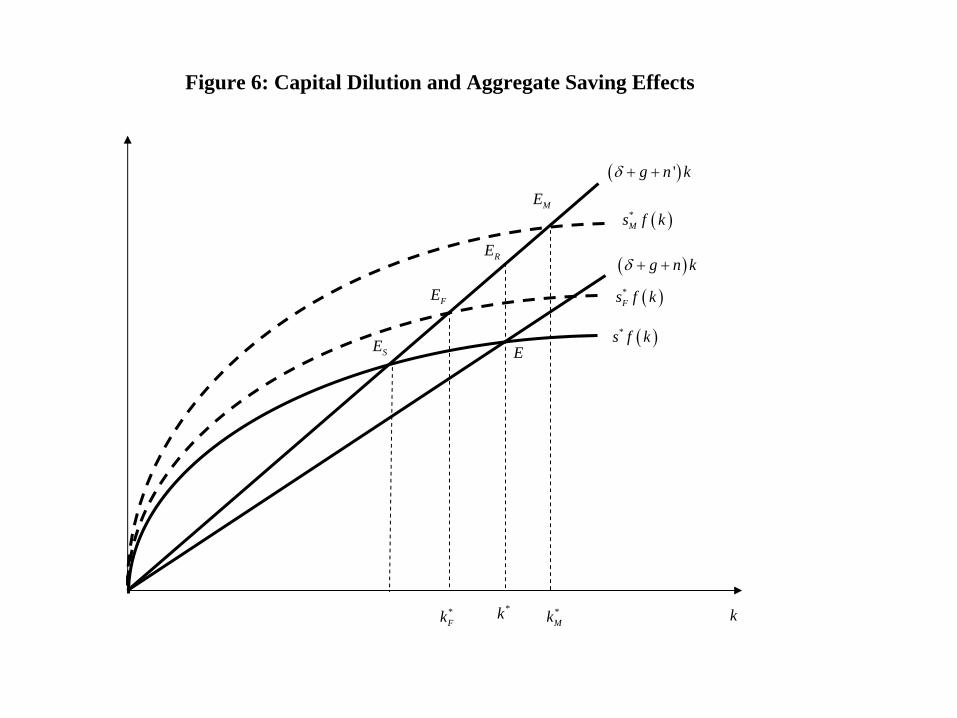
of (22) is represented by the concave curve s∗f (k) in Figure 6, where the equilibrium

aggregate saving rate s∗ = 20.58% for the benchmark case.15 The right-hand side

of (22) is represented by the straight line (δ + g + n) k, where n = −0.074%. Theintersection of the two curves gives the steady-state equilibrium of the OLG model,

denoted by point E in Figure 6.

We consider a fertility change and a mortality change such that the resulting popu-

lation growth rate is the same. Specifically, we consider a change of TFR from 2.05 to

2.064 (with life expectancy unchanged at 77.9) and a change of life expectancy from

77.9 to 81 (with TFR unchanged at 2.05). The first change is reported in the column

in italics in Table 1, and the second change in the column in italics in Table 2. In

each case, the population growth rate increases from n = −0.074% to n0 = −0.050%.Both of these changes are represented as an anti-clockwise rotation of the break-even

investment line to (δ + g + n0) k in Figure 6. As is well known in the economic growth

literature, the increase in population growth leads to a smaller capital per unit of ef-

fective labor (at the new equilibrium Es) if there is no change in the aggregate saving

rate, as in the Solow model. This is often called the capital dilution effect. However,

in general, aggregate saving does not remain unchanged with a demographic change.

In terms of the OLG model used in this paper, both individual saving behavior and

the age structure are affected. These two changes give rise to the aggregate saving

effect. As observed in Tables 1 and 2, aggregate saving rate increases slightly from

20.58% to 20.61% for the fertility change, but it rises more substantially from 20.58%

to 21.58% for the mortality change. For the fertility change, the rather small increase15Note that Figure 6 adopts the graphical approach of the Solow model, but unlikely that model,

the aggregate saving rate in our analysis is not constant when a fertility or mortality change causes

a rise in the population growth rate.

22

in aggregate saving leads to the result that the capital dilution effect dominates the

aggregate saving effect. As a result, the steady-state capital per unit of effective labor

decreases from k∗ to k∗F (at the new equilibrium EF ). On the other hand, for the

mortality change, the much larger increase in aggregate saving leads to the result that

the aggregate saving effect dominates the capital dilution effect and the steady-state

capital per unit of effective labor increases from k∗ to k∗M (at the new equilibrium

EM).16

Why does the aggregate saving rate increase more for the mortality change than for

the fertility change in Figure 6? It is useful to understand these general equilibrium

effects (with r∗, w∗ etc. changing in response to the exogenous shocks) by looking

at the life-cycle saving behavior and demographic characteristics. For the fertility

increase (i.e., a rise in TFR), the direct effect is a decrease in individual saving

(since each adult has more children and thus the household consumption expenditure

increases). A further look at the demographic structure suggests that the support

ratio increases. The net result of these opposing effects due to individual saving and

age structure turns out to be a small increase in aggregate saving.

The mortality reduction (i.e., an increase in life expectancy) in industrial countries

occurs mainly on older ages, instead of the young and child-bearing ages. As a

result, the support ratio decreases. On the other hand, individual saving increases in

response to a higher proportion of the lifetime expected to be in the post-retirement

years. Quantitatively, the increase in aggregate saving rate is very large, meaning

that the individual saving effect is substantially higher than the decrease through the

age-composition effect.16For the sake of completeness, we also label ER as the new equilibrium of the Ramsey-Cass-

Koopmans model when there is a rise in population growth rate. (In this case, the shift of the actual

investment schedule is not shown.)

23

7. CONCLUSION

To examine the economic consequences of fertility and mortality changes in in-

dustrial countries, we incorporate more realistic demographic features of age-specific

mortality rates, childhood and retirement years into a standard OLGmodel. We char-

acterize the steady-state equilibrium, and find that a fertility increase affects capital

accumulation negatively and a longevity increase affects it positively.

We decompose the economic effect of a fertility or mortality change into capital

dilution and aggregate saving effects. For a change in aggregate saving, which is due

to changes in the saving behavior of individuals weighted by the age distribution,

we further decompose it into individual saving and age-structure effects. For both

fertility and longevity increases, there is a negative capital dilution effect and a posi-

tive aggregate saving effect. Furthermore, there is a positive age-structure effect and

a negative individual saving effect for a fertility increase. On balance, it leads to

a small positive effect on aggregate saving and an overall negative effect on capital

accumulation. On the other hand, the longevity improvement in industrial countries

falls mainly on older ages, resulting in a negative age structure effect but a positive

individual saving effect. As mortality reduction falls mainly on retired senior citizens,

the increase in individual saving in response to this change is quite substantial, lead-

ing to a significant aggregate saving effect and an overall positive effect on capital

accumulation.17

One crucial ingredient of the current OLG model which leads to the above re-

sults is the exogenously fixed retirement age. While an unchanged retirement age17This point is closely related to Mason and Lee (2006), who argue that when individuals anticipate

a longer lifetime (and a larger proportion of time spent on retirement) in the future and save more

accordingly, there will be a beneficial effect on aggregate output through capital accumulation. They

call it the second demographic dividend, to distinguish it from the first demographic dividend which

is caused by the changes in age structure (Bloom and Williamson, 1998; Bloom et al., 2003).

24

seems to be a reasonable assumption for industrial countries in the last fifty years

or so, it is quite puzzling why the retirement age remains relatively unchanged when

there is a huge improvement in longevity. Moreover, it significantly affects the life-

cycle saving behavior when longevity improvement falls mainly on older ages when

most people retire. One possible extension in the future is to see what factors affect

the retirement decision, and to see whether the magnitude of the aggregate saving

changes in response to mortality reduction is substantially affected when retirement

decision is endogenous. In particular, Gruber and Wise (1998) argue that labor force

participation at old age is strongly affected by the provisions of the publicly-funded

pension scheme. It would be interesting to study the effects of longevity improvement

on individual retirement decision and aggregate saving under different institutional

arrangements of the social security program.

Another extension is to consider developing countries which are in an early stage

of demographic transition. In this case, it is helpful to relax the assumption of

exogenous fertility. One possibility is to consider fertility changes in response to

mortality reduction (as in Kalemli-Ozcan, 2003; Soares, 2005) when they fall mainly

on children and youth in developing countries. Endogenizing fertility choice not only

may provide methodological contribution to the research on economic-demographic

nexus, but also lead to a better understanding of many developing countries with

relatively high but declining fertility rates.

REFERENCES

[1] Abel, A. B (2003), “The effects of a baby boom on stock prices and capital accumu-

lation in the presence of social security,” Econometrica 71, 551-578.

[2] d’Albis, H. (2007), “Demographic structure and capital accumulation,” Journal of

Economic Theory 132, 411-434.

25

[3] Arthur, W. B. and G. McNicoll (1977), “Optimal time paths with age-dependence:

A Theory of population theory,” Review of Economic Studies 64, 111-123.

[4] Arthur, W. B. and G. McNicoll (1978), “Samuelson, population and intergenerational

transfers,” International Economic Review 19, 241-246.

[5] Auerbach, A. J. and L. J. Kotlikoff (1987), Dynamic Fiscal Policy. Cambridge Uni-

versity Press, New York, NY.

[6] Barro, R. J., N. G. Mankiw and X. Sala-i-Martin (1995), “Capital mobility in neo-

classical models of growth,” American Economic Review 85, 103-115.

[7] Blanchard, O. J. (1985), “Debt, deficits, and finite horizons,” Journal of Political

Economy 93, 223-247.

[8] Bloom, D. E. and J. G. Williamson (1998), “Demographic transition and economic

miracles in emerging Asia,” World Bank Economic Review 12, 419-455.

[9] Bloom, D. E., D. Canning and J. Sevilla (2003), The Demographic Dividend: A New

Perspective on the Economic Consequences of Population Change. CA: Santa

Monica: RAND.

[10] Bommier, A. and R. D. Lee (2003), “Overlapping generations models with realistic

demography,” Journal of Population Economics 16, 135-160.

[11] Boucekkine, R., D. de la Croix and O. Licandro (2002), “Vintage human capital,

demographic trends, and endogenous growth,” Journal of Economic Theory 104,

340-375.

[12] Buiter, W. H. (1988), “Death, birth, productivity growth and debt neutrality,” Eco-

nomic Journal 98, 279-293.

26

[13] Cass, D. (1965), “Optimum growth in an aggregative model of capital accumulation,”

Review of Economic Studies 32, 233-240.

[14] Centers for Disease Control and Prevention (2007), “Births: Final data for 2005,”

National Vital Statistics Reports Volume 56, Number 6.

[15] Coale, A. J. (1972), The Growth and Structure of Human Populations. Princeton:

Princeton University Press.

[16] Cutler, D. M., J. M. Poterba, L. M. Sheiner and L. H. Summers (1990), “An aging

society: Opportunity or challenge?” Brookings Papers on Economic Activity

1:1990, 1-73.

[17] Diamond, P. A. (1965), “National debt in a neoclassical growth model,” American

Economic Review 55, 1126-1150.

[18] Echevarria, C. A. and A. Iza (2006), “Life expectancy, human capital, social security

and growth,” Journal of Public Economics 90, 2323—2349.

[19] Ehrlich, I. and F. Lui (1997), “The problem of population and growth: A review of the

literature from Malthus to contemporary models of endogenous population and

endogenous growth,” Journal of Economic Dynamics and Control 21, 205—42.

[20] Faruqee, H. (2003), “Debt, deficits, and age-specific mortality,” Review of Economic

Dynamics 6, 300-312.

[21] Gan, Z and S.-H. P. Lau (2009), “Overlapping generations with age-specific mortality:

A simpler proof and less restrictive conditions,” Working Paper, University of

Hong Kong.

[22] Gruber, J. and D. Wise (1998), “Social security and retirement: An international

comparison,” American Economic Review Papers and Proceedings 88(2), 158—

163.

27

[23] Human Mortality Database (2008). University of California, Berkeley (USA), and

Max Planck Institute for Demographic Research (Germany). Available at

www.mortality.org (data downloaded on June 2008).

[24] Jones, C. J. (1995), “Time series tests of endogenous growth models,” Quarterly

Journal of Economics 110, 495-525.

[25] Kalemli-Ozcan, S. (2003), “A stochastic model of mortality, fertility, and human

capital investment,” Journal of Development Economics 70, 103-118.

[26] Keyfitz, N. and H. Caswell (2005), Applied Mathematical Demography, Third Edition.

New York: Springer Inc.

[27] Koopmans, T. C. (1965), “On the concept of optimal economic growth,” in The

Econometric Approach to Development Planning, pp. 225-287. Amsterdam:

North-Holland.

[28] Lau, S.-H. P. (2009), “Demographic structure and capital accumulation: A quantita-

tive assessment,” Journal of Economic Dynamics and Control 33, 554-567.

[29] Lee, R. D. and L. R. Carter (1992), “Modeling and forecasting U.S. mortality,” Jour-

nal of the American Statistical Association 87, 659-671.

[30] Lotka, A. J. (1939), Theorie analytique des associations biologiques. Part II. Hermann

et Cie, Paris, France. (Published in translation as: Analytical Theory of Biolog-

ical Populations, translated by D. P. Smith and H. Rossert. Plenum Press, New

York, 1998).

[31] Mason, A. and R. Lee (2006), “Reform and support systems for the elderly in de-

veloping countries: Capturing the second demographic dividend,” GENUS LXII

(2), 11-35.

28

[32] Oeppen, J. and J. W. Vaupel (2002), “Broken limits to life expectancy,” Science 269,

1029-1031.

[33] Ramsey, F. P. (1928), “A mathematical theory of saving,” Economic Journal 38,

543-559.

[34] Soares, R. R. (2005), “Mortality reductions, educational attainment, and fertility

choice,” American Economic Review 95, 580-601.

[35] Solow, R. M. (1956), “A contribution to the theory of economic growth,” Quarterly

Journal of Economics 70, 65-94.

[36] Weil, P. (1989), “Overlapping families of infinitely-lived agents,” Journal of Public

Economics 38, 183-198.

[37] Yaari, M. E. (1965), “Uncertain lifetime, life insurance, and the theory of the con-

sumer,” Review of Economic Studies 32, 137-150.

29

0 20 40 60 80 100

0.0

0.2

0.4

0.6

0.8

1.0

Figure 1: Percent Surviving (United States, 2005)

Age

Per

cent

0 20 40 60 80 100

−8

−6

−4

−2

0

Figure 2: Age−Specific Mortality Rates (United States, 1980 and 2005)

Age

log(

age−

spec

ific

mor

talit

y ra

te)

19802005

Figure 3: Time Line of Various Activities

Time

Age

s +Ωs ws T+bs T− b ws T T+ +

bs T+ rs T+

Ω

wT

0

Life Time (Probably up to ) Consumption Labor SupplyΩ

1.7 1.8 1.9 2.0 2.1

100

102

104

106

108

Figure 4: Fertility Change and Capital Accumulation

Total fertility rate

Ste

ady−

stat

e ca

pita

l per

uni

t of e

ffect

ive

labo

r (n

orm

aliz

ed)

76 78 80 82 84

9510

010

511

011

5

Figure 5: Life Expectancy and Capital Accumulation

Life expectancy at birth

Ste

ady−

stat

e ca

pita

l per

uni

t of e

ffect

ive

labo

r (n

orm

aliz

ed)

( )*s f k

( )*Ms f k

( )*Fs f k

( )'g n kδ + +

( )g n kδ + +

*k *Mk*

Fk

E

FE

ME

SE

k

RE

Figure 6: Capital Dilution and Aggregate Saving Effects

Table 1: Fertility Changes and Capital Accumulation

Total Fertility Rate 1.7 1.8 1.9 2 2.05 2.064 2.1

n (%)

Persons Aged 0-19 (%)

-0.743

19.77

-0.539

21.22

-0.346

22.65

-0.163

24.04

-0.074

24.72

-0.050

24.91

0.012

25.39

Persons Aged 65-110 (%)

26.28 24.61 23.07 21.66 21.00 20.82 20.37

Support Ratio (%) 59.87 60.60 61.21 61.72 61.93 61.99 62.13 Aggregate Saving Rate (%)

19.63 19.93 20.21 20.46 20.58 20.61 20.70

*k

5.123 4.999 4.888 4.786 4.739 4.727 4.694

Note: Support ratio = working-age population divided by equivalent adult consumers. The underlined cells (resp. cells not underlined) mean that the corresponding variable is decreasing (resp. increasing) in TFR.

Table 2: Mortality Changes and Capital Accumulation

Life Expectancy 75 77 77.9 79 81 83 85

n (%)

Persons Aged 0-19 (%)

-0.107

25.30

-0.083

24.90

-0.074

24.72

-0.065

24.48

-0.050

24.03

-0.038

23.57

-0.029

23.11

Persons Aged 65-110 (%)

19.13 20.42 21.00 21.75 23.12 24.50 25.88

Support Ratio (%) 63.62 62.46 61.93 61.27 60.07 58.87 57.67 Aggregate Saving Rate (%)

19.72 20.31 20.58 20.93 21.58 22.25 22.95

*k

4.488 4.659 4.739 4.844 5.044 5.259 5.487

Note: Support ratio = working-age population divided by equivalent adult consumers. The underlined cells (resp. cells not underlined) mean that the corresponding variable is decreasing (resp. increasing) in life expectancy.