Outlier Detection

Outlier detection is both easy and difficult.

• It is easy since there are several relatively straightforward tests for the presence of outliers.

• It is difficult since there are no firm rules as to when outlier removal is appropriate.

Outliers may be due to:

• Chance.

• Measurement error.

• Experimental error.

Outliers may or may not be a problem, depending on many factors:

• Some statistical tests are robust and can accommodate outliers, others may be severely influenced by outliers.▪ Parametric test can unduly influenced.▪ Non-parametric tests rarely are.

• Some data types will naturally contain extreme values.▪ Radiation levels often have extreme values (spikes).

• The presence of outliers may, in fact, be of interest.▪ Again, radiation spikes.

The outlier(s) may fall in a region of population overlap. This type of outlier must be removed from the data set.

Is this observation (57.00) an outlier?

In some cases a single outlier may influence normality, however, in this case the data are normal even with this observation.

Should this observation be examined further at this point?

Tests of Normality

Kolmogorov-Smirnova Shapiro-Wilk

Statistic df Sig. Statistic df Sig.

Male Standing-Sitting Height

Ratio (Cormic Index) .065 93 .200

* .986 93 .304

*. This is a lower bound of the true significance.

a. Lilliefors Significance Correction

Male Standing-Sitting Height Ratio (Cormic Index)

Stem-and-Leaf Plot

Frequency Stem & Leaf

1.00 Extremes (=<48.9)

3.00 49 . 446

12.00 50 . 012334557788

25.00 51 . 0122233344455566678888899

31.00 52 . 0111222233333334455555677789999

11.00 53 . 00111345789

7.00 54 . 0012378

2.00 55 . 02

1.00 Extremes (>=57.0)

Stem width: 1.00

Each leaf: 1 case(s)

The observation 57.0 is considered to be an extreme value in the stem and leaf plot.

When examining potential outliers, the detrended normal Q-Q plot is useful.

• Observations are transformed to z-scores and plotted as standard deviations from the mean.

This observation is nearly 1.5 standard deviations from the mean.

The best method of determining if an observation is an outlier is to use an outlier test.

• The test gives the probability that an observation is from a different population.

• It is defensible.

• It DOES NOT tell you whether or not to remove the extreme observation(s)…

s

xxGor

s

xxG min

minmax

max

Grubbs Outlier Test

where Gmax is used if the observation is greater than the mean and Gmin is used if it is less than the mean, and where xmax or xmin

is the extreme observation value.

From the G table at n=93 and α=0.05 the critical value is 3.18.

Since 3.49 > 3.18, reject Ho.

The observation is from a different population (G3.49, p < 0.025).

49.338.1

2.520.57

38.1

2.52

93

max

G

s

x

n

Ho: The observation is not different than the sample population.Ha: The observation is different than the sample population.

Critical Values of Grubb’s Outlier (G) TestTaken from Grubb 1969, Table 1

N α=0.05 α=0.025 α=0.01

Calculated value falls about here.

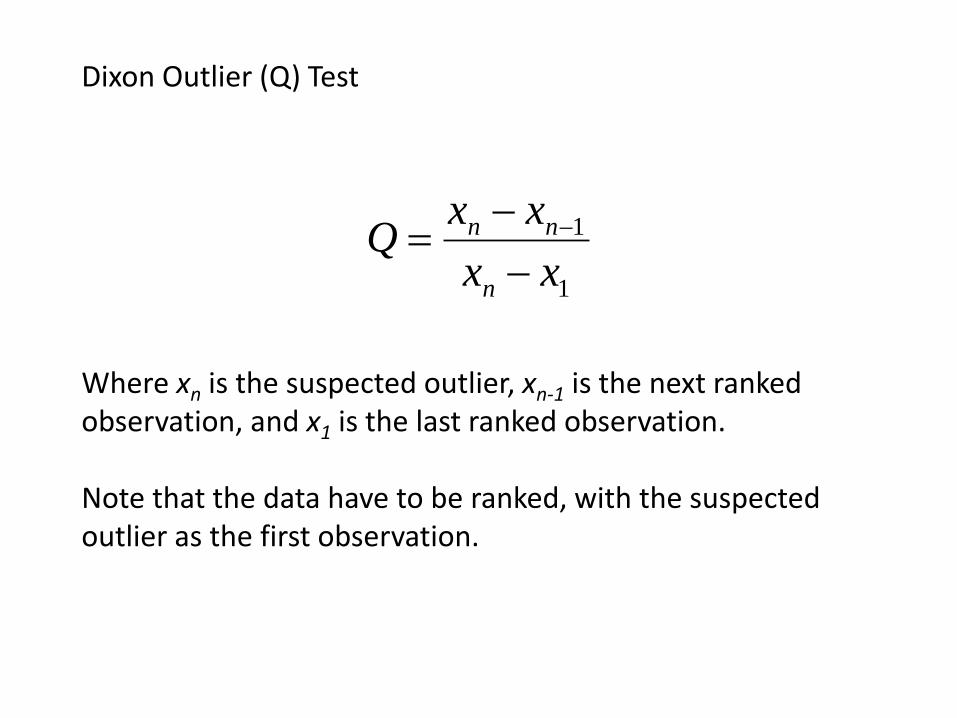
Dixon Outlier (Q) Test

Where xn is the suspected outlier, xn-1 is the next ranked observation, and x1 is the last ranked observation.

Note that the data have to be ranked, with the suspected outlier as the first observation.

1

1

xx

xxQ

n

nn

In SPSS Analyze > Descriptive Statistics > Explore, then choose the Statistics button and Outliers.

This gives the upper and lower extremes AND the next several observations, very useful when using the Dixon test.

Extreme Values

Case Number Value

Male Standing-Sitting Height

Ratio (Cormic Index)

Highest

1 1 57.00

2 2 55.20

3 3 55.06

4 4 54.87

5 5 54.72

Lowest

1 93 48.93

2 92 49.46

3 91 49.48

4 90 49.68

5 89 50.05

02.005.01881.0223.007.8

8.1

93.4800.57

20.5500.57

93

pQQ

n

Critical

Extreme Values

Case Number Value

Male Standing-Sitting Height

Ratio (Cormic Index)

Highest

1 1 57.00

2 2 55.20

3 3 55.06

4 4 54.87

5 5 54.72

Lowest

1 93 48.93

2 92 49.46

3 91 49.48

4 90 49.68

5 89 50.05

Ho: The observation is not different than the sample population.Ha: The observation is different than the sample population.

The observation is from a different population (Q 0.223, 0.05 > p > 0.02).

Characteristics of the Dixon and Grubbs Tests

Dixon Q:• Is the ratio of the ‘outlier gap’ to the data range.

• Similar to the w/s (range) normality test.

Grubbs G:• Is essentially a z score that references a modified t table.

• Very similar to a one-sample t test.

Suspect Cormic value becomes increasingly extreme.

More normal Less normal

The Grubbs test picks up extreme values earlier than the Dixon test, so choose the test that is most appropriate based on your knowledge of the data

The same data used the generate the previous graph, displayed as a detrendedQ-Q plot.

1 2 3

4 5 6

Final notes:

Outlier tests are an iterative process. 1. Check most extreme value for being an outlier.2. If it is, remove it.3. Check for the next extreme value using the new, smaller

sample.• It is smaller because the first outlier was removed.

4. Repeat the process.

Once all outlier are removed the sample can be analyzed.