Outlier Detection in Multivariate Time Series by...
16
Outlier Detection in Multivariate Time Series by Projection Pursuit Pedro GALEANO, Daniel PEÑA, and Ruey S. TSAY In this article we use projection pursuit methods to develop a procedure for detecting outliers in a multivariate time series. We show that testing for outliers in some projection directions can be more powerful than testing the multivariate series directly. The optimal directions for detecting outliers are found by numerical optimization of the kurtosis coefficient of the projected series. We propose an iterative procedure to detect and handle multiple outliers based on a univariate search in these optimal directions. In contrast with the existing methods, the proposed procedure can identify outliers without prespecifying a vector ARMA model for the data. The good performance of the proposed method is illustrated in a Monte Carlo study and in a real data analysis. KEY WORDS: Kurtosis coefficient; Level shift; Multivariate time series; Outlier; Projection pursuit. 1. INTRODUCTION Outlier detection in time series analysis is an important problem because the presence of even a few anomalous data can lead to model misspecification, biased parameter estima- tion, and poor forecasts. Several detection methods have been proposed for univariate time series, including those of Fox (1972), Chang and Tiao (1983), Tsay (1986, 1988), Chang, Tiao, and Chen (1988), Chen and Liu (1993), McCulloch and Tsay (1993, 1994), Le, Martin, and Raftery (1996), Luceño (1998), Justel, Peña, and Tsay (2000), Bianco, Garcia Ben, Martínez, and Yohai (2001), and Sánchez and Peña (2003). Most of these methods are based on sequential detection pro- cedures. For multivariate time series, Franses and Lucas (1998) studied outlier detection in cointegration analysis; Tsay, Peña, and Pankratz (2000) proposed a detection method based on individual and joint likelihood ratio statistics; and Lütkephol, Saikkonen, and Trenkler (2004) analyzed the effect of level shifts on the cointegration rank. Building adequate models for a vector time series is a diffi- cult task, especially when the data are contaminated by outliers. In this article we propose a method for identifying outliers with- out requiring initial specification of the multivariate model. The method is based on univariate outlier detection applied to some useful projections of the vector time series. The basic idea is simple: A multivariate outlier produces at least a univariate out- lier in almost every projected series, and by detecting the uni- variate outliers, we can identify the multivariate ones. We show that one can often better identify multivariate outliers by apply- ing univariate test statistics to optimal projections than by using multivariate statistics on the original series. We also show that in the presence of an outlier, the directions that maximize or minimize the kurtosis coefficient of the projected series include the direction of the outlier, that is, the direction that maximizes the ratio between the outlier size and the variance of the pro- jected observations. We propose an iterative algorithm based on projections to remove outliers from the observed series. Pedro Galeano is Teaching Assistant (E-mail: [email protected]) and Daniel Peña is Professor (E-mail: [email protected]), Department of Statistics, Carlos III de Madrid University, Madrid, Spain. Ruey S. Tsay is H. G. B. Alexander Professor of Econometrics and Statistics, Gradu- ate School of Business, University of Chicago, Chicago, IL 60637 (E-mail: [email protected]). The authors thank the referees and the asso- ciate editor for their excellent comments and suggestions. The first two au- thors acknowledge financial support by MEC grant SEJ2004-03303 and CAM grant HSE/0174/2004. The third author acknowledges financial support by Na- tional Science Foundation and the Graduate School of Business, University of Chicago. The article is organized as follows. In Section 2 we intro- duce some notation and briefly review the multivariate outlier approach presented by Tsay et al. (2000). In Section 3 we study properties of the univariate outliers introduced by multivariate outliers through projection and discuss some advantages of us- ing projections to detect outliers. In Section 4 we prove that the optimal directions to identify outliers can be obtained by max- imizing or minimizing the kurtosis coefficient of the projected series, and in Section 5 we discuss swamping and masking ef- fects. In Section 6 we propose an outlier detection algorithm based on projections. We generalize the procedure to nonsta- tionary time series in Section 7 and investigate the performance of the proposed procedure in a Monte Carlo study in Section 8. Finally, we apply the proposed method to a real data series in Section 9. 2. OUTLIERS IN MULTIVARIATE TIME SERIES Let X t = (X 1t ,..., X kt ) be a k-dimensional vector time series following the vector autoregressive moving average (VARMA) model (B)X t = C + (B)E t , t = 1,..., n, (1) where B is the backshift operator such that BX t = X t−1 , (B) = I − 1 B −···− p B p and (B) = I − 1 B −···− q B q are k × k matrix polynomials of finite degrees p and q, C is a k-dimensional constant vector, and E t = (E 1t ,..., E kt ) is a se- quence of independent and identically distributed (iid) Gaussian random vectors with mean 0 and positive-definite covariance matrix . For the VARMA model in (1), we have the AR repre- sentation (B)X t = C + E t , where (B) = (B) −1 (B) = I − ∑ ∞ i=1 i B i and C = (1) −1 C is a vector of constants if X t is invertible, and the MA representation X t = C + (B)E t , where (1)C = C and (B)(B) = (B) with (B) = I + ∑ ∞ i=1 i B i . Given an observed time series Y = (Y 1 ,..., Y n ) , where Y t = (Y 1t ,..., Y kt ) , Tsay et al. (2000) generalized four types of univariate outliers to the vector case in a direct manner using the representation Y t = X t + α(B)wI (h) t , (2) where I (h) t is a dummy variable such that I (h) h = 1 and I (h) t = 0 if t = h, w = (w 1 ,..., w k ) is the size of the outlier, and X t fol- © 2006 American Statistical Association Journal of the American Statistical Association June 2006, Vol. 101, No. 474, Theory and Methods DOI 10.1198/016214505000001131 654
Transcript of Outlier Detection in Multivariate Time Series by...
Outlier Detection in Multivariate Time Seriesby Projection Pursuit
Pedro GALEANO Daniel PENtildeA and Ruey S TSAY
In this article we use projection pursuit methods to develop a procedure for detecting outliers in a multivariate time series We show thattesting for outliers in some projection directions can be more powerful than testing the multivariate series directly The optimal directions fordetecting outliers are found by numerical optimization of the kurtosis coefficient of the projected series We propose an iterative procedureto detect and handle multiple outliers based on a univariate search in these optimal directions In contrast with the existing methods theproposed procedure can identify outliers without prespecifying a vector ARMA model for the data The good performance of the proposedmethod is illustrated in a Monte Carlo study and in a real data analysis
KEY WORDS Kurtosis coefficient Level shift Multivariate time series Outlier Projection pursuit
1 INTRODUCTION
Outlier detection in time series analysis is an importantproblem because the presence of even a few anomalous datacan lead to model misspecification biased parameter estima-tion and poor forecasts Several detection methods have beenproposed for univariate time series including those of Fox(1972) Chang and Tiao (1983) Tsay (1986 1988) ChangTiao and Chen (1988) Chen and Liu (1993) McCulloch andTsay (1993 1994) Le Martin and Raftery (1996) Lucentildeo(1998) Justel Pentildea and Tsay (2000) Bianco Garcia BenMartiacutenez and Yohai (2001) and Saacutenchez and Pentildea (2003)Most of these methods are based on sequential detection pro-cedures For multivariate time series Franses and Lucas (1998)studied outlier detection in cointegration analysis Tsay Pentildeaand Pankratz (2000) proposed a detection method based onindividual and joint likelihood ratio statistics and LuumltkepholSaikkonen and Trenkler (2004) analyzed the effect of levelshifts on the cointegration rank
Building adequate models for a vector time series is a diffi-cult task especially when the data are contaminated by outliersIn this article we propose a method for identifying outliers with-out requiring initial specification of the multivariate model Themethod is based on univariate outlier detection applied to someuseful projections of the vector time series The basic idea issimple A multivariate outlier produces at least a univariate out-lier in almost every projected series and by detecting the uni-variate outliers we can identify the multivariate ones We showthat one can often better identify multivariate outliers by apply-ing univariate test statistics to optimal projections than by usingmultivariate statistics on the original series We also show thatin the presence of an outlier the directions that maximize orminimize the kurtosis coefficient of the projected series includethe direction of the outlier that is the direction that maximizesthe ratio between the outlier size and the variance of the pro-jected observations We propose an iterative algorithm basedon projections to remove outliers from the observed series
Pedro Galeano is Teaching Assistant (E-mail pedrogaleanouc3mes)and Daniel Pentildea is Professor (E-mail danielpenauc3mes) Departmentof Statistics Carlos III de Madrid University Madrid Spain Ruey S Tsayis H G B Alexander Professor of Econometrics and Statistics Gradu-ate School of Business University of Chicago Chicago IL 60637 (E-mailrueytsaygsbuchicagoedu) The authors thank the referees and the asso-ciate editor for their excellent comments and suggestions The first two au-thors acknowledge financial support by MEC grant SEJ2004-03303 and CAMgrant HSE01742004 The third author acknowledges financial support by Na-tional Science Foundation and the Graduate School of Business University ofChicago
The article is organized as follows In Section 2 we intro-duce some notation and briefly review the multivariate outlierapproach presented by Tsay et al (2000) In Section 3 we studyproperties of the univariate outliers introduced by multivariateoutliers through projection and discuss some advantages of us-ing projections to detect outliers In Section 4 we prove that theoptimal directions to identify outliers can be obtained by max-imizing or minimizing the kurtosis coefficient of the projectedseries and in Section 5 we discuss swamping and masking ef-fects In Section 6 we propose an outlier detection algorithmbased on projections We generalize the procedure to nonsta-tionary time series in Section 7 and investigate the performanceof the proposed procedure in a Monte Carlo study in Section 8Finally we apply the proposed method to a real data series inSection 9
2 OUTLIERS IN MULTIVARIATE TIME SERIES
Let Xt = (X1t Xkt)prime be a k-dimensional vector time series
following the vector autoregressive moving average (VARMA)model
(B)Xt = C + (B)Et t = 1 n (1)
where B is the backshift operator such that BXt = Xtminus1 (B) =I minus 1B minus middot middot middot minus pBp and (B) = I minus 1B minus middot middot middot minus qBq
are k times k matrix polynomials of finite degrees p and q C is ak-dimensional constant vector and Et = (E1t Ekt)
prime is a se-quence of independent and identically distributed (iid) Gaussianrandom vectors with mean 0 and positive-definite covariancematrix For the VARMA model in (1) we have the AR repre-sentation (B)Xt = C + Et where (B) = (B)minus1(B) =I minus suminfin
i=1 iBi and C = (1)minus1C is a vector of constants ifXt is invertible and the MA representation Xt = C +(B)Et where (1)C = C and (B)(B) = (B) with (B) =I + suminfin
i=1 iBiGiven an observed time series Y = (Yprime
1 Yprimen)
prime whereYt = (Y1t Ykt)
prime Tsay et al (2000) generalized four typesof univariate outliers to the vector case in a direct manner usingthe representation
Yt = Xt + α(B)wI(h)t (2)
where I(h)t is a dummy variable such that I(h)
h = 1 and I(h)t = 0
if t = h w = (w1 wk)prime is the size of the outlier and Xt fol-
copy 2006 American Statistical AssociationJournal of the American Statistical Association
June 2006 Vol 101 No 474 Theory and MethodsDOI 101198016214505000001131
654
Galeano Pentildea and Tsay Outlier Detection by Projection Pursuit 655
lows a VARMA model The outlier type is defined by the ma-trix polynomial α(B) If α(B) = (B) then we have a multi-variate innovational outlier (MIO) if α(B) = I then we havea multivariate additive outlier (MAO) if α(B) = (1 minus B)minus1Ithen we have a multivariate level shift (MLS) and if α(B) =(I minus δIB)minus1 then we have a multivariate temporary (or transi-tory) change (MTC) where 0 lt δ lt 1 is a constant An MIO isan outlier in the innovations and can be interpreted as an inter-nal change in the structure of the series Its effect on the timeseries depends on the model and it can affect several consec-utive observations An MAO can be due to an external causesuch us a typo or measurement error and affects only a sin-gle observation An MLS changes the mean level of the seriesand thus it has a permanent effect An MTC causes an initialimpact but its effect decreases at a fixed rate in successive ob-servations In practice an outlier may produce a complex ef-fect given by a linear combination of the previously discussedpure effects Furthermore different components of Xt may suf-fer different outlier effects For instance an increase in energyprices can produce a transitory change in one country withouta permanent effect and a level shift in another country with apermanent effect An example of this kind of mixed effects isgiven in the real data example in Section 9
The effects of outliers on the innovations are easily obtainedwhen the parameters of the VARMA model for Xt are knownUsing the observed series and the known parameters of themodel for Xt we obtain a series of innovations At definedby At = (B)Yt minus C where Yt = Xt and At = Et for t lt hThe relationship between the true white noise innovations Etand the computed innovations At is given by
At = Et + (B)wI(h)t (3)
where (B) = (B)α(B) = I minus suminfini=1 iBi Tsay et al (2000)
showed that when the model is known the estimation of thesize of a multivariate outlier of type i at time h is given by
wih = minus(
nminushsum
j=0
primej
minus1j
)minus1(nminushsum
j=0
primej
minus1Ah+j
)
i = IALT
where 0 = minusI and we use the notation MIO equiv I MAO equiv AMLS equiv L and MTC equiv T for subscripts The covariance matrixof this estimate is ih = (
sumnminushj=0 prime
jminus1j)
minus1 and it is easy toshow that the multivariate test statistic
Jih = wprimeih
minus1ih wih i = IALT (4)
will be a noncentral χ2k (ηi) random variable with noncentral-
ity parameters ηi = wprimeminus1ih w for i = IALT In particular
under the null hypothesis H0 w = 0 the distribution of Jih
will be chi-squared with k degrees of freedom A second sta-tistic proposed by Tsay et al (2000) is the maximum compo-nent statistic defined by Cih = max|wjih|radicσjih 1 j ki = IALT where wjih is the jth element of wih and σjih isthe jth element of the main diagonal of ih
In practice the time index h of the outlier and the parame-ters of the model are unknown The parameter matrices are then
substituted by their estimates and the following overall test sta-tistics are defined
Jmax(ihi) = max1lehlen
Jih and
(5)Cmax(ihlowast
i ) = max1lehlen
Cih i = IALT
where hi and hlowasti denote the time indices at which the maximum
of the joint test statistics and the maximum component statisticsoccur
3 OUTLIER ANALYSIS THROUGH PROJECTIONS
In this section we explore the usefulness of projections of avector time series for outlier detection First we study the rela-tionship between the projected univariate models and the mul-tivariate model Second we discuss some potential advantagesof searching for outliers using the projected series
31 Projections of a VARMA Model
We begin with the properties of a univariate series obtainedby the projection of a VARMA series It is well known that anonzero linear combination of the components of the VARMAmodel in (1) follows a univariate ARMA model (see egLuumltkepohl 1993) Let xt = vprimeXt If Xt is a VARMA(pq)
process then xt follows an ARMA(plowastqlowast) model with plowast kpand qlowast (k minus 1)p + q In particular if Xt is a VMA(q) se-ries then xt is an MA(qlowast) with qlowast q and if Xt is a VAR(p)
process then xt follows an ARMA(plowastqlowast) model with plowast kpand qlowast (k minus 1)p A general form for the model of xt is
φ(B)xt = c + θ(B)et (6)
where φ(B) = |(B)| c = vprime(1)lowastC and vprime(B)Et = θ(B)et where (B)lowast is the adjoint matrix of (B) (B) = (B)lowast times(B) and et is a scalar white noise process with variance σ 2
e The values for θ(B) and σ 2
e can be obtained using the algorithmproposed by Maravall and Mathis (1994) that always gives aninvertible representation of the univariate process The AR rep-resentation of the univariate model (6) is π(B)xt = cπ + etwhere cπ = θ(1)minus1c and π(B) = θ(B)minus1φ(B) = 1minussuminfin
i=1 πiBiand its MA representation is xt = cψ + ψ(B)et where cψ =φ(1)minus1c and ψ(B) = φ(B)minus1θ(B) = 1 + suminfin
i=1 ψiBiWhen the observed series Yt is affected by an outlier
as in (2) the projected series yt = vprimeYt satisfies yt = xt +vprimeα(B)wI(h)
t Specifically if Yt has an MAO then the projectedseries is yt = xt + βI(h)
t so that it has an additive outlier of sizeβ = vprimew at t = h provided that vprimew = 0 In the same way theprojected series of a vector process with an MLS of size w willhave a level shift with size β = vprimew at time t = h The same re-sult also applies to an MTC Thus for the three types of outliersmentioned earlier the following hypotheses are equivalent
H0 w = 0
HA w = 0hArr Hlowast
0 β = 0
HlowastA β = 0
forallv isin Sk minus v perp w
because H0 = ⋃Hlowast0 v isin Sk minus v perp w where Sk = v isin R
k vprimev = 1
An MIO produces a more complicated effect It leads toa patch of consecutive outliers with sizes vprimew vprime1w
vprimenminushw starting with time index t = h Assuming that h isnot close to n and because j rarr 0 the size of the outlier in the
656 Journal of the American Statistical Association June 2006
patch tends to 0 In the particular case where vprime iw = ψivprimewforall i = 1 n minus h yt has an innovational outlier at t = h withsize β = vprimew But if vprime iw = 0 i = 1 n minus h then yt hasan additive outlier at t = h with size w and if vprime iw = vprimewi = 0 n minus h then yt has a level shift at t = h with sizeβ = vprimew Therefore the univariate series yt obtained by the pro-jection can be affected by an additive outlier a patch of outliersor a level shift
32 Some Advantages of Projection Methods
The first advantage of using projections to search multivari-ate outliers is simplicity By using univariate series we do notneed to prespecify a multivariate model for the underlying se-ries in outlier detection Second if the model parameters areknown then a convenient projection direction will lead to teststatistics that are more powerful than the multivariate onesThird as we show later in a Monte Carlo study the same con-clusion continues to hold when the parameters are estimatedfrom the observed series
To illustrate the second advantage consider a k-dimensionaltime series Yt generated from the VARMA model in (1) andaffected by an MAO MLS or MTC at t = h Let V be a k times kmatrix such that the first column is ww and the remainingcolumns consist of k minus 1 vectors that are orthogonal to w andhave unit length The multivariate series VprimeYt is affected by anoutlier of size (w0 0)prime at time t = h Note that the out-lier affects only the first component of the transformed seriesBecause the multivariate test statistic Jih of (4) is invariant tolinear transformations its value is the same for both Yt andVprimeYt series Thus all of the information concerning the outlieris in the first component of VprimeYt which is the projection of thevector time series in the direction of the outlier The remain-ing components of VprimeYt are irrelevant for detecting the out-lier Moreover because the test statistic Jih is distributed as a
noncentral χ2k (ηi) with noncentrality parameter ηi = wprimeminus1
ih wits power is given by Pow(M) = Pr(Jih gt χ2
kα) where χ2kα
is the 100αth percentile of the chi-squared distribution withk degrees of freedom In contrast projecting the series Yt ona given direction v we obtain a series yt affected by an out-lier at time t = h and the univariate test statistic jih = β2
ihσ2ih
where βih is a consistent estimate of β is distributed as a non-central χ2
1 (νi) with noncentrality parameter νi = β2σ 2ih where
β = vprimew and σ 2ih = var(βih) The power of this test statistic
is Pow(U) = Pr( jih gt χ21α) Because the detection procedure
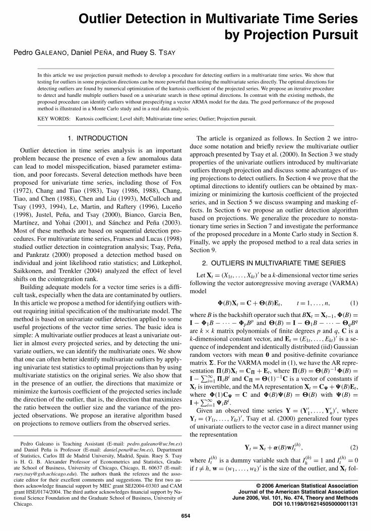
that we propose is affine equivariant for simplicity we assumethat Yt = Et is white noise and that = I If v = ww thenit is easy to see that for every w ηi = νi = wprimew for i = I AηL = νL = (nminush+1)wprimew and ηT = νT = (1minusδ2(nminush+1))(1minusδ2)wprimew The powers Pow(U) and Pow(M) and their differ-ences Pow(U) minus Pow(M) for the case of an MAO are shownin Figure 1 for different values of wprimew The figure shows thatthe larger the number of components the larger the advantageof the projection test over the multivariate one When the sizeof the outlier increases both tests have power close to 1 andhence the difference goes to 0 for large outliers In Section 8we show by a simulation study that for correlated series thesame conclusion will continue to hold when the parameters areestimated from the data although the power will depend on themodel
4 FINDING THE PROJECTION DIRECTIONS
The objective of projection pursuit algorithms is to find in-teresting features of high-dimensional data in low-dimensionalspaces via projections obtained by maximizing or minimizingan objective function termed the projection index which de-pends on the data and the projection vector It is commonly
(a)
(b)
Figure 1 Powers of the Multivariate and the Projection Statistics as a Function of the Outlier Size (a) Absolute powers (b) difference of powers
Galeano Pentildea and Tsay Outlier Detection by Projection Pursuit 657
assumed that the most interesting projections are the farthestones from normality showing some unexpected structure suchas clusters outliers or nonlinear relationships among the vari-ables General reviews of projection pursuit techniques havebeen given by Huber (1985) Jones and Sibson (1987) andPosse (1995) Pentildea and Prieto (2001a) proposed a procedurefor multivariate outlier detection based on projections that max-imize or minimize the kurtosis coefficient of the projected dataPentildea and Prieto (2001b) showed that these projected directionsare also useful to identify clusters in multivariate data PanFung and Fang (2000) suggested using projection pursuit tech-niques to detect high-dimensional outliers and showed that theprojected outlier identifier is a centered Gaussian process on ahigh-dimensional unit sphere Pan and Fang (2002) suggestedlooking for outliers in the projection directions given by the di-rections that maximizes the sample kurtosis and skewness
In this section we generalize the application of projectionsto multivariate time series analysis and define a maximum dis-crimination direction as the direction that maximizes the size ofthe univariate outlier vprimew with respect to the variance of theprojected series We show that for an MAO MLS and MTCthe direction of the outlier is a direction of maximum discrimi-nation which can be obtained by finding the extremes of thekurtosis coefficient of the projected series For an MIO weprove that the direction of the outlier is a maximum discrimina-tion direction for the innovations series which can be obtainedby projecting the innovations
In what follows for a time series zt we define z = 1n
sumnt=1 zt
and zt = zt minus z where n is the sample size Let Yt and At bethe observed series and innovations in (2) and (3) For easein presentation and without loss of generality we assume thatE(Xt) = 0 and X = cov(Xt) = I and define the determinis-tic variable Rt = α(B)wI(h)
t Projecting Yt on the direction vwe obtain yt = xt + rt where rt = vprimeRt In addition we haveE[ 1
n
sumnt=1 Yt] = E(Y) = R and
Y = E
[1
n
nsum
t=1
(Yt minus Y)(Yt minus Y)prime]
= E
[1
n
nsum
t=1
YtYprimet
]
= I + R
where R = 1n
sumnt=1 RtRprime
t Using the results of Rao (1973p 60) the maximum of (vprimew)2(vprimeYv) under the constraintvprimeYv = 1 is v = Yw For the cases of MAO MLS andMTC we have Y = I + βiwwprime with βi given by
βA = n minus 1
n2
βL = n minus h + 1
n
(h minus 1
n
)
βT = 1
n
[(1 minus δ2(nminush+1)
1 minus δ2
)
minus 1
n
(1 minus δ(nminush+1)
1 minus δ
)2]
and v = (1 + βiwprimew)w Thus the interesting direction v of pro-jection is proportional to w The same result also holds in theMIO case for the maximum of (vprimew)2(vprimeAv) under the con-straint vprimeAv = 1 where A is the expected value of the co-variance matrix of the innovations At
We prove next that the direction of the outlier w can befound by maximizing or minimizing the kurtosis coefficient of
the projected series Toward this end we need some preliminaryresults the proofs of which are given in the Appendix
Lemma 1 The kurtosis coefficient γy(v) of the project seriesyt = vprimeYt under the restriction vprimeYv = 1 is
γy(v) = 3 minus 3(vprimeRv)2 + ωr(v) (7)
where ωr(v) = 1n
sumnt=1 r4
t
Lemma 2 The extreme directions of the kurtosis coefficientof yt under the constraint vprimeYv = 1 are given by the eigen-vectors of the matrix
sumnt=1 βt(v)RtRprime
t associated with eigen-values micro(v) = n(vprimeRv)2(γr(v) minus 3) where βt(v) = (vprimeRt)
2 minus3(vprimeRv) minus micro(v)n and γr(v) is the kurtosis coefficient ofrt = vprimeRt Moreover the directions that maximize or minimizethe kurtosis coefficient are given by the eigenvectors associatedwith the largest and the smallest eigenvalues micro(v)
The following theorem shows the usefulness of the extremedirections of the kurtosis coefficient of yt
Theorem 1 Suppose that Xt is a stationary VARMA( pq)process and Yt = Xt + α(B)wI(h)
t as in (2) then we have thefollowing results
a For an MAO the kurtosis coefficient of yt is maximizedwhen v is proportional to w and is minimized when v is orthog-onal to w
b For an MTC the kurtosis coefficient of yt is maximizedor minimized when v is proportional to w and is minimized ormaximized when v is orthogonal to w
c For an MLS the kurtosis coefficient of yt is minimizedwhen v is proportional to w and is maximized when v is or-thogonal to w if
h isin(
1 + 1
2
(
1 minus 1radic3
)
n1 + 1
2
(
1 + 1radic3
)
n
)
Otherwise the kurtosis coefficient of yt is maximized when v isproportional to w and is minimized when v is orthogonal to w
Theorem 1 has two important implications First for anMAO MLS or MTC one of the directions obtained by max-imizing or minimizing the kurtosis coefficient is the directionof the outlier Second these directions are obtained without theinformation of the time index at which the outlier occurs Giventhe characteristics of innovational outliers it is natural to thinkthat the direction of the outlier can be obtained by focusing onthe innovations series This is indeed the case
Corollary 1 If Xt is a stationary VARMA( pq) process andYt = Xt + (B)wI(h)
t as in (2) with At = Et + wI(h)t then the
kurtosis coefficient of at = vprimeAt is maximized when v is pro-portional to w and is minimized when v is orthogonal to w
5 MASKING AND SWAMPING EFFECTS
In the presence of multiple outliers it would be of limitedvalue if one considered only the projections that maximize orminimize the kurtosis coefficient because of the potential prob-lem of masking effects For instance a projection might effec-tively reveal one outlier but almost eliminate the effects of otheroutliers To overcome such a difficulty we present an iterative
658 Journal of the American Statistical Association June 2006
procedure for analyzing a set of 2k orthogonal directions con-sisting of (a) the direction that maximizes the kurtosis coeffi-cient (b) the direction that minimizes the kurtosis coefficientand (c) two sets of k minus 1 directions orthogonal to (a) and (b)Our motivation for using these orthogonal directions is twofoldFirst the results of Section 4 reveal that in some cases the di-rections of interest are orthogonal to those that maximize orminimize the kurtosis coefficient of the projected series sec-ond these directions ensure nonoverlapping information sothat if the effect of an outlier is almost hidden in one directionthen it may be revealed by one of the orthogonal directionsFurthermore after removing the effects of outliers detected inthe original set of 2k orthogonal directions we propose to iter-ate the analysis using new directions until no more outliers aredetected Therefore if a set of outliers are masked in one direc-tion then they may be revealed either in one of the orthogonaldirections or in a later iteration after removing detected outliersTo illustrate we analyze in detail the cases of a series with twoMAOs and an MAO and an MLS
Theorem 2 Suppose that Xt is a stationary VARMA( pq)process Yt is the observed vector series and yt = vprimeYt is a pro-jected scalar series
a Let Yt = Xt +w1I(h1)t +w2I(h2)
t with h1 lt h2 There arethree possibilities as follows
1 If w1 and w2 are proportional to each other then the kur-tosis coefficient of yt is maximized when v is proportionalto wi and is minimized when v is orthogonal to wi
2 If w1 and w2 are orthogonal then the kurtosis coefficientis maximized when v is proportional to the outlier withlarger Euclidean norm and minimized when v is in one ofthe orthogonal directions
3 Let ϕ be the angle between w1 and w2 then the kur-tosis coefficient is approximately maximized when v isthe direction of the outlier that gives the maximum ofw1w2 cosϕw2w1 cosϕ where the quan-tity denotes the ratio between the norm of outlier wi andthe length of the projection of outlier wj on wi wherej = i
b Let Yt = Xt + w1I(h1)t + w2S(h2)
t with h1 lt h2 Then thekurtosis coefficient of yt is maximized or minimized when v isproportional to w2 and it is minimized or maximized when v isorthogonal to w2
In the case of two MAOs Theorem 2 shows that if both out-liers are proportional then the maximum of the kurtosis co-efficient is obtained in the direction of the outliers and if theoutliers are orthogonal then the maximum of the kurtosis is ob-tained in the direction of the outlier with larger Euclidean normand the minimum is obtained in an orthogonal direction Thusan orthogonal direction of the one that gives the maximum ofthe kurtosis coefficient will reveal the presence of the outlierwith smaller norm If the outliers are neither proportional nororthogonal to each other then the direction of the outlier withthe largest projection on the direction of the other outlier willproduce a maximum kurtosis coefficient Note that the projec-tion of w2 on the direction of w1 is given by w2 cosϕ Theratio w1w2 cosϕ is large if w1 is large enough com-pared with w2 in which case the kurtosis coefficient will be
maximized in the direction of w1 or if cosϕ is small enoughin which case an orthogonal direction to w1 will reveal w2
Second the direction of the MLS gives the maximum orthe minimum of the kurtosis coefficient of the projected seriesThus the MLS will be revealed in the directions that maximizeor minimize the kurtosis coefficient of yt Projecting in the or-thogonal directions will eliminate the effect of this level shiftand reveal the second outlier If the statistics for this secondoutlier are not significant then we remove the effect of the levelshift and a new set of directions may reveal the second outlier
In contrast outlier detection procedures are sometimes af-fected by swamping effects that is one outlier affects the seriesin such a way that other ldquogoodrdquo data points appear like outliersThe procedure that we propose in the next section includes sev-eral steps to avoid swamping effects which can appear in theunivariate searches using the projection statistics The idea isto delete nonsignificant outliers after a joint estimation of theparameters and detected outliers We clarified this in the nextsection
6 ALGORITHMS FOR OUTLIER DETECTION
Here we propose a sequential procedure for outlier detectionbased on the directions that mimimize and maximize the kur-tosis coefficient of the projections We refer to these directionsas the optimal projections The procedure is divided into foursteps (1) Obtain these directions (2) search for outliers in theprojected univariate time series (3) remove the effect of all de-tected outliers by using an approximated multivariate modeland (4) iterate the previous steps applied to the cleaned seriesuntil no more outliers are found Note that in step 2 the detec-tion is carried out in two stages First MLSs are identified andsecond MIOs MAOs and MTCs are found Finally a vectormodel is identified for the cleaned time series and the outliereffects and model parameters are jointly estimated The fittedmodel is refined if necessary for example removing insignifi-cant outliers if any
61 Computation of the Projection Directions
We use the procedure of Pentildea and Prieto (2001b) to constructthe 2k projection directions of interest For an observed vectorseries Yt our goal here is to obtain the maximum and mini-mum of the kurtosis coefficient of the projected series and theorthogonal directions of the optimal projections Toward thisend consider the following procedure
1 Let m = 1 and Z(m)t = Yt
2 Let (m)Z = 1
n
sumnt=1 Z(m)
t Z(m)primet and find vm such that
vm = arg maxvprime
m(m)Z vm=1
1
n
nsum
t=1
(vprime
mZ(m)t
)4 (8)
3 If m = k then stop otherwise define Z(m+1)t = (I minus
vmvprimem
(m)Z )Z(m)
t that is Z(m+1)t is the projection of
the observations in an orthogonal direction to vm Letm = m + 1 and go to step 2
4 Repeat the same procedure to minimize the objectivefunction in (8) to obtain another set of k directionsnamely vk+1 v2k
Galeano Pentildea and Tsay Outlier Detection by Projection Pursuit 659
A key step of the foregoing algorithm is to solve theoptimization problem in (8) Toward this end we use amodified Newton method to solve the system given by thefirst-order optimality conditions nablaγz(v) minus 2λ
(m)Z v = 0 and
vprime(m)Z v minus 1 = 0 by means of linear approximations (See Pentildea
and Prieto 2001b for technical details of the method) One rel-evant issue is that the proposed procedure is affine equivariantthat is the method selects equivalent directions for series mod-ified by an affine transformation
62 Searching for Univariate Outliers
The most commonly used tests for outlier detection in uni-variate time series are the likelihood ratio test (LRT) statis-tics λih i = IALT (see Chang and Tiao 1983 Tsay 1988)Because the location of the outlier and the parameters of themodel are unknown the estimated parameters are used to de-fine the overall test statistics (ihi) = max|λit|1 le t le ni = IALT Using these statistics Chang and Tiao (1983)proposed an iterative algorithm for detecting innovational andadditive outliers Tsay (1988) generalized the algorithm to de-tect level shifts and transitory changes (see Chen and Liu 1993Saacutenchez and Pentildea 2003 for additional extensions)
In this article we consider a different approach There is sub-stantial evidence that using the same critical values for all theLRT statistics can easily misidentify a level shift as an innova-tive outlier (see Balke 1993 Saacutenchez and Pentildea 2003) The latterauthors showed that the critical values for the LRT statistic fordetecting level shifts are different from those for testing addi-tive or innovative outliers Therefore we propose to identify thelevel shifts in a series before checking for other types of outlierToward this end it is necessary to develop a procedure that iscapable of detecting level shifts in the presence of the othertypes of outliers Using the notation of Section 31 Bai (1994)proposed the cusum statistic
Ct = tradicnψ(1)σe
(1
t
tsum
i=1
yi minus y
)
(9)
to test for a level shift at t = h+1 in a linear process and showedthat the statistic converges weakly to a standard Brownianbridge on [01] In practice the quantity ψ(1)σe is replacedby a consistent estimator
ψ(1)σe =[
γ (0) + 2Ksum
i=1
(
1 minus |i|K
)
γ (i)
]12
where γ (i) = cov( yt ytminusi) and K is a quantity such thatK rarr infin and Kn rarr 0 as n rarr infin Under the assumption ofno level shifts in the sample the statistic max1letlen |Ct| is as-ymptotically distributed as the supremum of the absolute valueof a Brownian bridge with cumulative distribution functionF(x) = 1 + 2
suminfini=1(minus1)ieminus2i2x2
for x gt 0 The cusum statis-tic (9) has several advantages over the LRT statistic for detect-ing level shifts First it is not necessary to specify the orderof the ARMA model which can be difficult in the presence oflevel shifts Second as shown in Section 8 this statistic seemsto be more powerful than the LRT in all the models consideredThird the statistic (9) seems to be robust to the presence ofother outliers whereas the LRT statistic is not
621 Level Shift Detection Given the 2k projected uni-variate series yti = vprime
iYt for i = 1 2k we propose an it-erative procedure to identify level shifts based on the algorithmproposed by Inclaacuten and Tiao (1994) and Carnero Pentildea andRuiz (2003) for detecting variance changes and level shifts in awhite noise series Let H be the prespecified minimum distancebetween two level shifts The proposed algorithm divides theseries into pieces after detecting a level shift and proceeds asfollows
1 Let t1 = 1 and t2 = n Obtain
DL = max1leile2k
maxt1letlet2
|Cit| (10)
where Cit is the statistic (9) applied to the ith projected
series for i = 1 2k Let
(imax tmax) = arg max1leile2k
arg maxt1letlet2
|Cit| (11)
If DL gt DLα where DLα is the critical value for thesignificance level α then there is a possible level shift att = tmax + 1 and we go to step 2a If DL lt DLα thenthere is no level shift in the series and the algorithmstops
2a Define t2 = tmax of step 1 and obtain new values of DLand (imax tmax) of (10) and (11) If DL gt DLα and t2 minustmax gt H then we redefine t2 = tmax and repeat step 2auntil DL lt DLα or t2 minus tmax le H Define tfirst = t2 wheret2 is the last time index that attains the maximum of thecusum statistic that is larger than DLα and satisfies t2 minustmax gt H The point tfirst + 1 is the first time point with apossible level shift
2b Define t1 = tmax of step 1 and t2 = n and obtain new val-ues of DL and (imax tmax) of (10) and (11) If DL gt DLα
and tmax minus t1 gt H then we redefine t1 = tmax and re-peat step 2b until DL lt DLα or tmax minus t1 le H Definetlast = t1 where t1 is the last time index that attains themaximum of the cusum statistics that is larger than DLα
and satisfies tmax minus t1 gt H The point tlast + 1 is the lasttime point with a possible level shift
2c If tlast minus tfirst lt H then there is just a level shift and thealgorithm stops If not then keep both values as possi-ble changepoints and repeat steps 2a and 2b for t1 = tfirstand t2 = tlast until no more possible changepoints are de-tected Then go to step 3
3 Define a vector hL = (hL0 hL
rL+1) where hL0 = 1
hLrL+1 = n and hL
1 lt middot middot middot lt hLrL
are the changepoints de-tected in step 2 Obtain the statistic DL in each subin-terval (hL
i hLi+2) and check its statistical significance If
it is not significant then eliminate the correspondingpossible changepoint Repeat step 3 until the number ofpossible changepoints remains unchanged and the timeindexes of changepoints are the same between iterationsRemoving hL
0 = 1 and hLrL+1
= n from the final vector oftime indexes we obtain rL level shifts in the series attime indexes hL
i + 1 for i = 1 L4 Let hL
1 hLrL
be the time indexes of rL detected levelshifts To remove the impacts of level shifts we fit themodel
(I minus 1B minus middot middot middot minus pBp)Ylowastt = Alowast
t (12)
660 Journal of the American Statistical Association June 2006
where Ylowastt = Yt minussumrL
i=1 wiS(hL
i )t and the order p is chosen
such that
p = arg max0leplepmax
AIC(p) = arg max0leplepmax
log |p| + 2k2p
n
where p = 1nminus2pminus1
sumnt=p+1 Alowast
t Alowastprimet and pmax is a pre-
specified upper bound If some of the effects of levelshifts are not significant then we remove the least sig-nificant one from the model in (12) and reestimate theeffects of the remaining rL minus 1 level shifts This processis repeated until all of the level shifts are significant
Some comments on the proposed procedure are in orderFirst the statistic DL is the maximum of dependent randomvariables and has an intractable distribution We obtain criti-cal values by simulation in the next section Second the teststatistics (9) are highly correlated for close observations Thusconsecutive large values of Ct might be caused by a single levelshift To avoid overdetection we do not allow two level shiftsto be too close by using the number H in steps 2 and 3 In thesimulations and real data example we chose H = 10 and foundthat it works well
622 An Algorithm for Outlier Detection Using the level-shift adjusted series we use the following procedure to detectadditive outliers transitory changes and innovative outliers inthe 2k projected univariate series yti = vprime
iYlowastt and their associ-
ated innovational series ati = vprimeiA
lowastt for i = 1 2k
1 For each projected series yti fit an AR( p) with p selectedby the Akaike information criterion (AIC) and computethe LRT statistics λi
At and λiTt In addition compute the
LRT statistics λiIt using the associated innovational se-
ries ati This leads to the maximum statistics
A = max1leile2k
max1letlen
|λiAt|
T = max1leile2k
max1letlen
|λiTt| and (13)
I = max1leile2k
max1letlen
|λiIt|
2 For i = AT and I let Aα Tα and Iα be the crit-ical values for a predetermined significance level α Ifi lt iα for i = IAT then no outliers are found andthe algorithm stops If i gt iα for only one i then iden-tify an outlier of type i and remove its effect using themultivariate parameter estimates If i gt iα for morethan one i then identify the outlier based on the most sig-nificant test statistic and remove its effect using the multi-variate parameter estimates Repeat steps 1 and 2 until nomore outliers are detected
3 Let hA1 hA
rA hT
1 hTrT
and hI1 hI
rI be the
time indexes of the rA rT and rI detected additive out-liers transitory changes and innovative outliers Estimatejointly the model parameters and the detected outliers forthe series Ylowast
t (I minus 1B minus middot middot middot minus pBp)Ylowastlowastt = Alowastlowast
t where
Ylowastlowastt = Ylowast
t minusrAsum
iA=1
wiA I(hA
iA)
t minusrTsum
iT=1
wiT
1 minus δBI(hT
iT)
t
and
Alowastlowastt = Alowast
t minusrIsum
iI=1
wiI I(hI
iI)
t
If some of the outlier effects become insignificant thenremove the least significant outlier and reestimate themodel Repeat this process until all of the remaining out-liers are significant
In Section 8 we obtain critical values for the test statis-tics λi
At λiTt and λi
It through simulation
63 Final Joint Estimation of ParametersLevel Shifts and Outliers
Finally we perform a joint estimation of the model parame-ters the level shifts and the outliers detected using the equation(I minus 1B minus middot middot middot minus pBp)Zt = Dt where
Zt = Yt minusrLsum
iL=1
wiL S(hL
iL)
t minusrAsum
iA=1
wiA I(hA
iA)
t minusrTsum
iT=1
wiT
1 minus δBI(hT
iT)
t
and
Dt = At minusrIsum
iI=1
wiI I(hI
iI)
t
and hL1 hL
rL hA
1 hArA
hT1 hT
rT and hI
1 hIrI
are the time indexes of the rL rA rT and rI detected level shiftsadditive outliers transitory changes and innovative outliers Ifsome effect is found to be not significant at a given level thenwe remove the least significant one and repeat the joint estima-tion until all of the effects are significant
Some comments on the proposed procedure are as followsFirst as mentioned in Section 2 an outlier can be a combina-tion of different effects This does not cause any problem forthe proposed procedure because it allows for multiple outlierdetections at a given time point either in different projectiondirections or in successive iterations The real data example ofSection 9 demonstrates how the proposed procedure handlessuch a situation Second the procedure includes several stepsto avoid swamping effects Specifically after detecting levelshifts we fit an autoregression and remove any nonsignificantlevel shifts We repeat the same step after detecting the othertypes of outlier Finally we perform a joint estimation of modelparameters and detected level shifts and outliers to remove anynonsignificant identification of level shift or outliers
7 THE NONSTATIONARY CASE
In this section we study the case when the time series isunit-root nonstationary Assume that Xt sim I(d1 dk) wherethe dirsquos are nonnegative integers denoting the degrees of dif-ferencing of the components of Xt Let d = max(d1 dk)
and consider first the case of d = 1 which we denote simplyby Xt sim I(1) For such a series in addition to the outliers in-troduced by Tsay et al (2000) we also entertain the multi-variate ramp shift (MRS) defined as Yt = Xt + wR(h)
t whereR(h)
t = (I minus B)minus1S(h)t with S(h)
t being a step function at the timeindex h (ie S(h)
t = 1 if t ge h and = 0 otherwise) This out-lier implies a slope change in the multivariate series and it may
Galeano Pentildea and Tsay Outlier Detection by Projection Pursuit 661
occur in an I(1) series It is not considered in the stationarycase because the series has no time slope Consequently for anMRS we assume that it applies only to the components of Ytwith dj = 1 that is the size of the outlier w = (w1 wk)
primesatisfies wj = 0 if dj = 0
The series Xt can be transformed into stationarity by tak-ing the first difference of its components even though dj mightbe zero for some j As we show later this is not a drawbackfor our method The first differencing affects the existing out-liers as follows In the MIO case (I minus B)Yt = (I minus B)Xt +(B)wI(h)
t where (B) = (I minus B)(B) Therefore an MIOproduces an MIO in the differenced series In the MAO case(I minus B)Yt = (I minus B)Xt + w(I(h)
t minus I(h)tminus1) producing two consec-
utive MAOs with the same size but opposite signs In the MLScase (IminusB)Yt = (IminusB)Xt +wI(h)
t resulting in an MAO of thesame size In the MTC case (IminusB)Yt = (IminusB)Xt +ζ(B)wI(h)
t where ζ(B) = 1 + ζ1B + ζ2B2 + middot middot middot such that ζj = δjminus1(1 minus δ)Thus an MTC produces an MTC with decreasing coefficients ζj
In the MRS case (I minus B)Yt = (I minus B)Xt + wS(h)t which pro-
duces an MLS with same sizeThe results of Section 4 can be extended to include the
aforementioned outliers induced by differencing For instanceTheorem 1 shows that the directions that maximize or minimizethe kurtosis coefficient of the projected series under the pres-ence of two consecutive MAOs with the same size but oppositesigns are the direction of the outlier or a direction orthogonal toit Therefore in the I(1) case we propose a procedure similarto that of the stationary case for the first differenced series Thisprocedure consists of the following steps
1 Take the first difference of all of the components of YtCheck for MLS as in Section 621 All of the level shiftsdetected in the differenced series are incorporated as rampshifts in the original series and are estimated jointly withthe model parameters If any ramp shift is not significantthen remove it from the model and repeat the detectingprocess until all of the ramp shifts are significant Thisleads to a series Ylowast
t = Yt minus sumrRi=1 wiR
(h)t that is free of
ramp shifts2 Take the first difference of all of the components of Ylowast
t The series (I minus B)Ylowast
t may be affected by MIOs two con-secutive MAOs MAOs and MTCs Then proceed as inSection 622 All of the outliers detected in the differ-enced series are incorporated by the corresponding effectsin the original series and are estimated jointly with themodel parameters If any of the outliers becomes insignif-icant then remove it from the model Repeat the processuntil all of the outliers are statistically significant
The procedure can also be applied to series that have dj = 0for some components and to cointegrated series In thesecases nablaYt is overdifferenced implying that its MA componentcontains some unit roots Nevertheless this is not a problem forthe proposed procedure If the series is not cointegrated thenany projection direction provides an univariate series withoutunit roots in its MA component If the series is cointegratedthen the directions of the outliers will in general be differentfrom the directions of cointegration In other words if v is avector obtained by maximizing or minimizing the kurtosis co-efficient then it is unlikely to be a cointegration vector and
vprimenablaYt = nabla(vprimeYt) is stationary and invertible because vprimeYt isa nonstationary series However if the series are cointegratedthen the final estimation should be carried out using the errorcorrection model of Engle and Granger (1987) Note that if v isthe cointegration vector then vprimeYt is stationary and nablavprimeYt isoverdifferenced Although no relationship is expected betweenthe outlier directions and the cointegration vector we have ver-ified by using Monte Carlo simulations that the probabilityof finding the cointegration relationship as a solution of theoptimization algorithm is very low Specifically we generated10000 series from a vector AR(1) model with two componentsand a cointegration relationship and found the directions in (8)To compare the directions with the cointegration vector wecalculated the absolute value of the cosine of the angle be-tween these two directions The average value of this cosineis 62 with variance 09 It is easy to show that if the angle hasa uniform distribution in the interval (0π) then the distribu-tion of the cosine of the angle has mean 63 and variance 09Next we repeated the same experiment with the same seriesbut affected by outliers level shifts or transitory changes andobtained in every case that the mean of the angles between thedirection found and the cointegrating direction is the one thatexits between the direction of the outlier and the cointegrationdirection Therefore we conclude that there should be no con-fusion between the cointegration vectors and the directions thatmaximize or minimize the kurtosis coefficient of the projectedseries
Consider next the case where d = 2 Define a multivari-ate quadratic shift (MQS) as Yt = Xt + wQ(h)
t where Q(h)t =
(I minus B)minus1R(h)t This outlier introduces a change in the quadratic
trend of the multivariate series The series Xt can be trans-formed into a stationary one by taking the second differencesHence an MQS is transformed into an MLS an MRS is trans-formed into an MAO and so on A similar procedure as thatproposed for the I(1) case applies In fact the discussion canbe generalized to handle outliers in a general I(d) series
8 SIMULATIONS AND COMPUTATIONAL RESULTS
In this section we investigate the computational aspects of theproposed procedures through simulation First we obtain criti-cal values for all of the test statistics second we compare thepower of the multivariate and projection procedures for detect-ing outliers We begin with the power of detecting level shiftsfollowed by power of identifying other types of outlier To savespace we show only the results for the stationary case
81 Critical Values
Critical values of the test statistics for outlier detection forunivariate and multivariate time series are usually obtainedthrough simulation using a numerous series from different mod-els For instance the outlier detection routines in the pro-grams TRAMO and SCA use critical values obtained by sucha simulation study We follow this stream and consider eightVARMA( pq) models to generate the critical values The di-mensions used in the simulation are k = 235 and 10 and theparameter matrices used are given in Table 1 The constant termof the models is always the vector 1k and the innovations co-variance matrix is the identity matrix For cases of k = 2 and 3the AR parameter matrices have eigenvalues of approximately
662 Journal of the American Statistical Association June 2006
Table 1 Vector Time Series Models Used in Simulation Study
Model
1 2 3
Dimension k = 2
[6 22 4
] [6 22 4
]
[minus7 0minus1 minus3
] [minus7 0minus1 minus3
]
Model
4 5 6
Dimension k = 3
[6 2 02 4 06 2 5
] [6 2 02 4 06 2 5
]
[minus7 0 0minus1 minus3 0minus7 0 minus5
] [minus7 0 0minus1 minus3 0minus7 0 minus5
]
Model 7
Dimension k = 5 diag() = (9 7 5 3 1) and (i i + 1) = minus5 i = 1 4
(i j) = 0 elsewhere
Model 8
Dimension k = 10 diag() = (9 8 1 0) and (i i + 1) = minus5 i = 1 9
(i j) = 0 elsewhere
276 and 724 and 276 5 and 724 whereas the MA para-meter matrices have eigenvalues minus3 and minus7 and minus3minus5and minus7 For the cases where k = 5 and 10 the AR parametermatrices have nonzero elements in their main and first upper di-agonals only and their eigenvalues are the elements of their re-spective main diagonals Using the eight models we generatedcritical values of the test statistics IAL and T in (13)and DL in (10) The LRT statistic for detecting level shifts isincluded for comparison purposes
The sample sizes used are n = 50100200300400and 500 covering most of the cases encountered in practiceFor a given model and sample size we generated 10000 se-ries and computed the test statistics Table 2 summarizes theempirical critical values of the simulation From this table wesee only minor differences in the critical values among dif-ferent models of the same dimension and hence recommendthe critical values in Table 3 for practical use In applicationif the sample size is different from those used in the simula-tion then we recommend interpolating the values of Table 3To better understand the relationship between critical valuesand the number of components and sample size we fitted threelinear regressions in which each column of critical values inTable 3 at the 95th percentile serving as the dependent vari-ables with the number of components k and the number ofobservations n as the regressors The fitted regressions arei = 324 + 1561k + 0014n L = 286 + 0780k + 0008nand DL = 121+ 0240k + 0005n for i = IAT All estimatedparameters are statistically significant and the R2 of the regres-sions are 97 94 and 82 We used these three regressions toobtain critical values for various samples sizes and numbersof components and found that a small increase in the samplesize produced a small increase in the critical values The threeregressions work well in general
Finally we also obtained critical values for the multivariatetest statistics in (5) through the same simulation method forsample sizes n = 100 and 200 Table 4 shows the recommendedcritical values for practical use These critical values are used inpower comparisons of the next section
82 Power and Robustness Comparison of the Statisticsfor Detecting Level Shifts
Next we compare the performance of the multivariate LRTstatistics the test statistics based on projections and the cusumtest for detecting level shifts We use sample sizes n = 100and 200 and three different outlier sizes wL = 3 times 1k 4 times 1kand a random wL The direction of the random wL is generatedby drawing a uniform [01] random variable u for each com-ponent of wL and defining wLi = 0 or 3 if u is in the interval(012) or (121) If wLi = 0 for all i then we discard theoutlier
For a given sample size and level shift we generated 1000series and computed the test statistic Jmax in (5) for a level shiftthe maximum projection statistic L in (13) and the maximumcusum statistic in (10) based on the proposed procedure Wecompare each statistic with its critical values in Tables 3 and 4at the 5 significance level and tabulate the number of times alevel shift is detected The results are given in the first part ofTable 5 (see columns Jmax L and DL) For all of the mod-els considered the cusum test outperforms the other two butall three tests seem to have good power when the sample sizeis 200
We also study the power of these three statistics in the pres-ence of other outliers Specifically for each model we gener-ated 1000 series of size n = 100 Each series is contaminatedby an MIO at hI = 20 with size wI = w times 1k an MAO athA = 40 with size wA = minusw times 1k an MTC at hT = 80 with sizewT = minusw times 1k and an MLS at hL = 60 with size wL = w times 1kwhere w = 3 or 4 A random vector w generated by the samemethod as before is also used as the size for all outliers Wecompute and compare the three test statistics of level shift withtheir respective critical values in Tables 3 and 4 at the 5 sig-nificance level The power of these three statistics are given inthe second part of Table 5 (see columns Jmax L and DL)All three tests are affected by the presence of other outliers butsimilar to the case of a single level shift the cusum test contin-ues to outperform the other two test statistics Furthermore wemeasured the power loss of each test by
loss(i) = 1 minus power with outliers in model i
power with no outliers in model i
and obtained the mean power loss of the three test statistics forthe eight models used with w = 3 The average losses for themultivariate statistic the projection statistic and the cusum testare 241 133 and 54 Therefore the multivariate andprojection test statistics for level shift seem to be more suscep-tible to masking effects than the cusum test statistic
Finally we study the robustness properties of these statisticsin the presence of other outliers With this objective we obtainthe empirical type I error and compare it with the nominal levelof the test We use a generating procedure similar to that of thepower study to conduct the simulation However for each gen-erated series the outliers consist of an MIO at hI = 25 with size
Galeano Pentildea and Tsay Outlier Detection by Projection Pursuit 663
Table 2 Empirical Critical Values of the Test Statistics Considered
95th percentiles 99th percentiles
n k M ΛI ΛA ΛL ΛT DL ΛI ΛA ΛL ΛT DL
50 2 1 353 348 291 347 126 381 375 324 376 1322 347 347 287 334 126 390 376 317 370 1333 357 341 297 344 125 392 384 326 372 132
3 4 390 377 308 370 128 410 394 341 391 1355 385 371 294 365 129 413 394 349 394 1366 389 366 307 370 128 411 391 345 393 135
5 7 420 392 334 377 131 445 424 369 402 136
10 8 492 467 375 430 134 513 489 421 456 139
100 2 1 375 371 308 364 134 408 403 340 406 1442 375 361 306 359 133 415 398 345 398 1433 376 362 308 363 134 412 402 350 406 143
3 4 403 380 319 378 137 439 410 350 415 1455 408 391 316 377 136 445 409 349 414 1456 400 378 316 375 136 436 406 356 410 145
5 7 449 414 347 413 144 477 451 384 449 151
10 8 530 494 382 479 149 559 528 425 510 153
200 2 1 401 392 315 395 141 428 424 354 429 1502 397 388 318 384 140 420 419 350 428 1493 395 384 321 380 140 425 411 349 410 150
3 4 427 405 325 407 143 477 439 369 446 1555 434 409 325 406 142 477 444 358 450 1546 432 398 329 404 142 469 434 371 437 155
5 7 469 432 356 433 154 504 470 394 466 167
10 8 553 513 384 507 162 593 557 427 542 174
300 2 1 405 403 325 400 143 432 431 365 430 1562 407 393 322 401 142 430 427 366 430 1553 404 392 326 398 143 434 434 372 425 156
3 4 438 418 338 411 147 473 450 379 453 1615 438 417 332 417 146 480 461 364 452 1606 436 413 338 417 147 472 450 377 460 160
5 7 482 445 363 448 154 531 479 399 483 170
10 8 562 522 389 511 167 599 560 430 546 181
400 2 1 413 408 341 409 144 450 447 383 447 1582 417 405 342 405 145 462 437 377 450 1573 419 405 338 413 144 464 439 378 460 158
3 4 436 424 345 426 147 489 461 393 470 1625 444 434 354 424 148 479 471 385 465 1616 444 421 348 420 148 486 465 389 452 162
5 7 490 447 360 451 157 538 489 405 488 173
10 8 569 524 392 515 168 603 568 432 553 182
500 2 1 418 419 346 421 145 462 454 384 445 1602 418 413 342 411 146 460 452 382 453 1593 418 407 346 414 145 448 448 382 450 159
3 4 446 428 350 426 149 491 471 396 472 1625 451 432 353 432 148 498 473 391 475 1636 444 431 356 425 149 493 467 391 467 163
5 7 495 453 365 457 159 540 492 410 501 178
10 8 577 525 395 519 169 606 570 435 558 184
NOTE These values are based on sample size n and 10000 realizations M denotes the models in Table 1
wI = w times 1k an MAO at hA = 50 with size wA = minusw times 1k andan MTC at hT = 75 with size wT = w times 1k where w = 3 or 4Again we also used a random vector w generated as beforefor the size of all outliers The last eight rows of Table 5 givethe frequencies that the test statistic is greater than its empiri-cal 95th percentile of Tables 3 and 4 These frequencies denotechances of a false detection of a level shift by the three statis-tics Once again the cusum statistic outperforms the other twoin maintaining the size of a test and being robust to the other
types of outliers The multivariate and projection statistics seemnot robust to the presence of other outliers
83 Power Comparison of the Multivariate andUnivariate Statistics for Other Outliers
In this section we investigate the power of the test statisticsfor detecting other types of outlier The outliers considered areMAOs MIOs and MTCs Again we used the eight models inTable 1 and sample sizes n = 100 and 200 The outlier occurs
664 Journal of the American Statistical Association June 2006
Table 3 Recommended Critical Values of the Test StatisticsConsidered for Sample Size n
95th percentiles 99th percentiles
n k ΛI ΛA ΛT ΛL DL ΛI ΛA ΛT ΛL DL
50 2 35 29 126 38 32 1333 38 30 128 40 34 1355 40 33 131 42 37 136
10 46 37 134 49 42 139
100 2 37 31 134 41 34 1433 39 32 136 42 35 1455 42 34 144 46 39 151
10 50 38 149 53 42 153
200 2 39 32 140 42 36 1503 41 33 142 45 37 1555 44 36 154 48 39 167
10 52 38 162 56 43 174
300 2 40 33 143 43 37 1563 42 34 147 46 38 1605 46 36 154 50 41 170
10 53 39 167 57 43 181
400 2 41 34 144 45 38 1583 43 35 148 47 39 1625 46 36 157 51 42 173
10 54 39 168 58 43 182
500 2 42 34 145 45 38 1593 43 35 149 48 39 1635 47 37 159 51 41 178
10 55 40 169 59 44 184
at t = n2 and assumes three possible sizes as before For eachcombination of model sample size and outlier we generated1000 series to compute the proposed test statistics We thencompared the statistics with their empirical 95th percentiles ofTables 3 and 4 and tabulated the frequencies of detecting a sig-nificant outlier Table 6 summarizes the power of various teststatistics From this table it seems that projection test statis-tics outperform their corresponding multivariate counterpartsOverall our limited simulation study supports the use of pro-jections and cusum statistics in detecting outliers in a vectortime series
9 AN ILLUSTRATIVE EXAMPLE
We illustrate the performance of the proposed proceduresby analyzing a real example The data are the logarithms ofthe annual gross national product (GNP) of Spain Italy andFrance denoted by S I and F from 1947 to 2003 The serieshave 57 observations and are depicted by solid lines in Fig-ure 2 Because the GNP are clearly nonstationary we take thefirst difference of each series We then compute the projection
directions using the proposed procedure of Section 6 and ap-ply the level shift detection algorithm to detect ramp shifts inthe original series The critical value is chosen by means ofthe regressions in Section 81 and turns out to be 132 Thealgorithm detects a ramp shift at time hL
1 = 1975 The valueof the test statistic (10) for the time index is 139 To esti-mate the effect of the ramp shift we first check whether theseries are cointegrated using Johansenrsquos test (Johansen 1991)We find a cointegration vector β and we use the AIC to selectthe error correction model with a cointegrating vector given bynablaYt = D1nablaYtminus1 minus αβ primeYtminus1 + At where the estimated para-meters are
D1 =(
299 095 510
069 344 524
100 221 728
)
α =(
007minus001003
)
and
β =( 10762
minus2235511975
)
Note that this model is equivalent to the VAR(2) modelYt = 1Ytminus1 + 2Ytminus2 + At with 1 = I + D1 minus αβ prime and2 = minusD1 Then using this model we remove the effect ofthe ramp shift by estimating the regression model At = (I minus1B minus 2B2)wR(1975)
t + Et and obtain the series free from theeffect of the ramp shift by Ylowast
t = Yt minus wR(1975)t
Next we consider the detection of other types of outlier Thecritical value is chosen using the fitted regression of Section 81and turns out to be 38 The first part of Table 7 summarizes theresults of the detection procedure It identifies an MLS in 1966and its effect on the series is removed as in the case of the MRSThe procedure then detects an MAO in 1975 which is estimatedand cleaned from the series The procedure fails to detect anyother outliers and is terminated The outlier-adjusted series areshown by dashed lines in Figure 2
After identifying the outliers for the series we estimatejointly the outlier effects and the model parameters using a first-order vector error correction model with a cointegration rela-tionship The estimated effects of the three detected outliersalong with the t-ratios of the estimates are given in Table 8The ramp shift detected by the algorithm in 1975 implies a de-crease in the rate of GNP growth of about 2 in the three coun-tries with the largest in Italy (minus22) and smallest in Spain
Table 4 Empirical Critical Values of the Multivariate Statistics Considered
95th percentiles 99th percentiles
n k Jmax (I) Jmax (A) Jmax (L) Jmax (T) Jmax (I) Jmax (A) Jmax (L) Jmax (T)
100 2 140 135 95 136 161 157 113 1633 160 158 117 154 183 181 136 1845 189 192 144 187 215 223 173 214
10 254 258 192 267 276 287 218 267
200 2 155 159 108 157 185 194 134 1893 178 183 129 180 207 208 159 2035 218 223 166 217 254 256 200 242
10 298 303 217 296 333 345 257 331
Galeano Pentildea and Tsay Outlier Detection by Projection Pursuit 665
Table 5 Empirical Power of Multivariate Projection and Cusum Test Statistics for Detecting a Level Shift
w = 3 times 1k w = 4 times 1k w = random
n k M hI hA hL hT Jmax ΛL DL Jmax ΛL DL Jmax ΛL DL
100 2 1 50 700 830 100 966 982 100 530 829 9922 2 50 583 826 100 892 969 100 526 810 9932 3 50 465 733 876 915 932 100 414 700 8633 4 50 936 927 996 100 988 100 604 710 9843 5 50 681 988 100 947 997 100 275 953 1003 6 50 863 866 887 989 990 992 283 836 8815 7 50 433 981 986 837 998 998 333 750 856
10 8 50 286 938 964 727 969 983 150 802 809
200 2 1 100 807 954 100 981 996 100 743 839 1002 2 100 922 956 100 970 993 100 861 934 1002 3 100 781 906 995 971 984 100 731 872 9723 4 100 987 989 100 100 100 100 922 747 1003 5 100 858 998 100 990 100 100 837 966 1003 6 100 975 978 100 996 997 100 808 958 1005 7 100 709 998 999 947 999 100 735 757 976
10 8 100 694 100 100 973 100 100 532 865 961
100 2 1 20 40 60 80 456 760 926 730 918 993 450 778 9292 2 20 40 60 80 520 876 100 743 967 100 637 874 1002 3 20 40 60 80 170 536 666 403 843 866 356 704 1003 4 20 40 60 80 736 740 903 920 850 100 473 645 9063 5 20 40 60 80 613 816 100 713 920 100 780 915 1003 6 20 40 60 80 636 553 743 870 800 950 256 794 9985 7 20 40 60 80 143 860 874 173 904 939 254 593 847
10 8 20 40 60 80 32 584 746 27 619 798 60 581 716
100 2 1 25 50 75 40 140 33 26 263 33 35 150 452 2 25 50 75 3 90 30 13 110 20 7 80 172 3 25 50 75 40 213 43 23 313 46 9 105 273 4 25 50 75 63 156 30 70 280 63 43 193 413 5 25 50 75 33 80 40 23 126 43 3 90 273 6 25 50 75 163 223 43 166 273 46 19 123 395 7 25 50 75 34 361 45 44 495 55 58 317 48
10 8 25 50 75 46 448 43 39 604 46 45 389 33
NOTE n is the sample size M denotes the model in Table 1 hi denotes time point at which a type i outlier occurs and w is the outlier
Table 6 Empirical Power of Multivariate and Projection Test Statistics for Detecting an Outlier in a Vector Time Series
n = 100 h = 50 n = 200 h = 100
w = 3 times 1k w = 4 times 1k w = random w = 3 times 1k w = 4 times 1k w = random
k M Jmax ΛI Jmax ΛI Jmax ΛI Jmax ΛI Jmax ΛI Jmax ΛI
MIO2 1 599 778 950 980 442 659 588 718 926 968 426 5612 2 539 715 898 953 364 581 585 684 925 955 387 5282 3 511 686 880 952 405 612 570 683 927 956 424 5403 4 819 915 996 992 463 745 816 875 100 100 483 6673 5 620 761 951 974 332 700 674 762 977 985 342 6403 6 618 781 923 976 385 702 671 758 982 988 428 6385 7 954 997 100 100 587 914 967 993 100 100 575 825
10 8 996 100 100 100 697 997 981 100 100 100 804 984
MAO2 1 866 936 993 993 583 863 873 936 993 100 552 7432 2 670 960 960 100 389 876 670 910 956 993 356 7572 3 910 990 996 100 444 877 980 980 100 100 362 6913 4 983 993 996 100 686 849 993 996 100 100 661 6933 5 786 956 986 100 375 863 826 896 990 990 377 7533 6 970 990 996 100 397 912 988 978 100 100 463 8085 7 911 994 100 100 749 935 975 975 100 100 726 848
10 8 992 100 100 100 816 971 100 100 100 100 901 953
MTC2 1 613 886 933 986 461 826 610 886 980 980 418 7832 2 645 970 940 100 588 937 660 920 946 993 621 8712 3 713 936 926 993 577 867 736 903 977 986 608 8183 4 900 980 100 100 594 849 920 928 995 995 549 6813 5 710 976 953 996 670 914 753 933 993 100 617 7733 6 826 956 970 986 524 882 959 957 100 992 539 8155 7 972 996 100 100 694 884 992 100 100 100 711 802
10 8 972 100 100 100 763 974 994 100 100 100 813 947
NOTE n is the sample size M denotes the model in Table 1 h is the time index of outlier and w is the size of the outlier
666 Journal of the American Statistical Association June 2006
(a)
(b)
(c)
Figure 2 Original ( mdashndash) and Modified ( - - - -) Logarithms of the GNP of (a) Spain (b) Italy and (c) France
(minus167) The detected shift can be associated with the firstoil crisis In fact the ramp shift is visible from the plot of theseries The proposed algorithm also identifies an MAO in 1975indicating that the first year of the oil crisis also had a transitoryeffect that was most important in Italy (minus67) As mentionedin Section 6 the proposed procedure allows for multiple outlierdetections at a time point In this case one MRS affecting all ofthe components and one MAO affecting primarily the GNP ofItaly are found The final fitted vector error correction model is
nablaYt =(
2856 1839 3461
0341 6710 2721minus0912 3765 5778
)
nablaYtminus1
minus(
007minus000002
)
(14412 minus21651 8132 )Ytminus1 + At
There are marked changes in the parameter estimates ofthe model with and without outlier detection For instancesubstantial changes in the diagonal elements of the D1 ma-trix are observed before and after the outlier detection for theItalian and French GNP The estimates of the cointegration vec-tor also change The estimated long-run equilibrium relation-ship between the variables before outlier detection is roughly(5S + 5F) minus I After outlier modeling the cointegration vec-tor becomes roughly (64S + 36F) minus I which gives heavierweight to the Spanish GNP
Finally we compare the results with those obtained by ap-plying the procedure of Tsay et al (2000) We obtained criticalvalues for the multivariate test statistics in a simulation not re-ported here using the models in Table 1 The 5 critical valuesfor the multivariate statistics are 173 for MIO MAO and MTCand 148 for MLS The critical values for the component statis-tics are 39 for MIO MAO and MTC and 36 for MLS The
Table 7 Outliers Found by the Proposed Algorithm and the Tsay Pentildea and Pankratz Procedure
Proposed procedureIterations (ΛI hI ) (ΛA hA) (ΛL hL) (ΛT hT ) Time Type
1 (411 1966) (405 1965) (478 1966) (422 1966) 1966 MLS2 (337 1976) (477 1975) (415 1975) (445 1975) 1975 MAO3 (314 1960) (374 1960) (349 1960) (368 1960)
Procedure of Tsay Pentildea and PankratzIterations (JI hI ) (JA hA) (JL hL) (JT hT ) Time Type
1 (1508 1966) (1554 1965) (1139 1975) (1411 1966)
Iterations (CI hI ) (CA hA) (CL hL) (CT hT ) Time Type
2 (378 1966) (384 1965) (316 1975) (342 1966)
Galeano Pentildea and Tsay Outlier Detection by Projection Pursuit 667
Table 8 Estimation of the Sizes of the Outliers Detectedby the Algorithm
S I FTime Type (t-ratio) (t-ratio) (t-ratio)
1966 MLS 0165 0473 0152(17046) (70546) (20114)
1975 MRS minus0167 minus0224 minus0196(minus19723) (minus24668) (minus22817)
1975 MAO minus0434 minus0672 minus0312(minus18392) (minus41121) (minus16917)
second part of Table 7 summarizes the results using the samefirst-order vector error correction model The procedure fails todetect any outliers at the 5 level even though some of the teststatistics are only slightly smaller than the critical values
APPENDIX PROOFS
Proof of Lemma 1
Taking into account that yt = xt + rt xt and rt are independent thatE[xt] = E[x3
t ] = 0 and recalling that y = 1n
sumni=1 yi
E[( yt minus y)4] = E[(xt + rt)4] = E[x4
t ] + 6E[x2t ]r2
t + r4t
As vprimeYv = 1 the kurtosis coefficient of y is given by
γy(v) = 1
n
nsum
t=1
(E[x4
t ] + 6E[x2t ]r2
t + r4t)
Finally as E[x2t ] = vprimev E[x4
t ] = 3E[x2t ]2 = 3(vprimev)2 1
nsumn
t=1 r2t =
vprimeRv and vprimev = vprimeYv minus vprimeRv we obtain γy(v) = 3(vprimeYv)2 minus3(vprimeRv)2 + ωr(v)
Proof of Lemma 2
The Lagrangian for the extreme points of γy(v) is pound(v) = 3 minus3(vprimeRv)2 + ωr(v) minus λ(vprimeYv minus 1) with gradient
nablapound(v) = minus12(vprimeRv)Rv +(
4
n
nsum
t=1
r2t RtRprime
t
)
v minus 2λYv
Letting nablapound(v) equal 0 multiplying by vprime in the equality and takinginto account the constraint vprimeYv = 1 we have λ = minus6(vprimeRv)2 +2ωr(v) Because R = 1
nsumn
t=1 RtRprimet we have
minus12(vprimeRv)Rv + 4
(1
n
nsum
t=1
r2t RtRprime
t
)
v
=(
minus12(vprimeRv)2 + 4
n
nsum
t=1
r2t
)
(I + R)v
Therefore
minus3(vprimeRv)Rv + 3(vprimeRv)2Rv +(
1
n
nsum
t=1
r2t RtRprime
t
)
v
minus 1
n
nsum
t=1
r2t Rv = minus3(vprimeRv)2v + 1
n
nsum
t=1
r2t v
and finally
nsum
t=1
[
r2t minus 3(vprimeRv) minus micro(v)
n
]
RtRprimetv = n(vprimeRv)2(γr(v) minus 3)v
Thus the extreme directions of pound(v) under vprimeYv = 1 are theeigenvectors of the matrix
sumnt=1 βt(v)RtRprime
t with eigenvalues micro(v) =
n(vprimeRv)2(γr(v)minus3) where βt(v) = [(vprimeRt)2 minus3(vprimeRv)minusmicro(v)n]
From (7) we get that γy(v) = 3 minusσ 4r (3 minusγr(v)) = 3 +micro(v)n There-
fore the maximum or the minimum of γy(v) will be given when micro(v)
is as large or as small as possible and the maximum and the minimumof the kurtosis will be given by the maximum and the minimum of theeigenvalues of the matrix
sumnt=1 βt(v)RtRprime
t
Proof of Theorem 1
We use the equalities vprimeRv = 1n
sumnt=1 r2
t and (vprimeRv)2γr(v) =1n
sumnt=1 r4
t
a For an MAO rh = vprimew rt = 0 forall t = h and r = rhn Firstn(vprimeRv)2γr(v) = c1r4
h and vprimeRv = c2r2h where
c1 =(
1 minus 1
n
)[(
1 minus 1
n
)3+ 1
n3
]
c2 = 1
n
(
1 minus 1
n
)
and the eigenvalues are given by micro(v) = c0r4h where c0 = c1 minus 3nc2
2In contrast after some algebra it can be shown that
[ nsum
t=1
βt(v)RtRprimet
]
v = [m1r3h + m2r5
h]Rh (A1)
where
m1 =(
1 minus 1
n
)[1
n3+
(
1 minus 1
n
)3minus 3c2
]
m2 = minusc01
n
(
1 minus 1
n
)
Because Rh = w
v = m1r3h + m2r5
h
c0r4h
w
and the other eigenvectors are orthogonal to w Moreover because theeigenvalues are given by c0r4
h and c0 gt 0 for n gt 5 we get that themaximum of the kurtosis coefficient is given in the direction of wwhereas the minimum is attained in the orthogonal directions to w
b For an MTC rt = 0 if t lt h rt = δtminushrh for t ge h and r = mrhwhere m = (1 minus δnminush+1)(n(1 minus δ)) First n(vprimeRv)2γr(v) = c1r4
hand vprimeRv = c2r2
h where
c1 = (h minus 1)m4 +nsum
t=h
(δtminush minus m)4
c2 = 1
n
[
(h minus 1)m2 +nsum
t=h
(δtminush minus m)2
]
and the eigenvalues are given by micro(v) = c0r4h where c0 = c1 minus 3nc2
2In contrast after some algebra it can be shown that the relation (A1)is valid in this case for the values
m1 = (h minus 1)(m4 minus 3c2m2) +nsum
t=h
[(δtminush minus m)4 minus 3c2(δtminush minus m)2]
m2 = minus c0
n
[
(h minus 1)m2 +nsum
t=h
(δtminush minus m)2
]
and one eigenvector is proportional to w and the others are orthogonalto it Because the eigenvalues are given by c0r4
h the kurtosis coeffi-cient of yt is maximized or minimized when v is proportional to wdepending on the sign of c0 which in general depends on the valuesof n h and δ
c For an MLS rt = 0 if t lt h rt = rh for t ge h and r = nminush+1n rh
First n(vprimeRv)2γr(v) = c1r4h and vprimeRv = c2r2
h where
c1 = (h minus 1)(n minus h + 1)
n4[(n minus h + 1)3 + (h minus 1)3]
c2 = (h minus 1)(n minus h + 1)
n2
668 Journal of the American Statistical Association June 2006
and the eigenvalues are given by micro(v) = c0r4h where c0 = c1 minus 3nc2
2In contrast after some algebra it can be shown that the relation (A1)is valid in this case for the values
m1 = (h minus 1)(n minus h + 1)
n4
[(n minus h + 1)3 + (h minus 1)3 minus 3c2
]
and
m2 = minusc0(h minus 1)(n minus h + 1)
n2
showing that one eigenvector is proportional to w and the others are or-thogonal to it The eigenvalues are given by c0r4
h and it is not difficultto see that c0 lt 0 if and only if
h isin(
1 + 1
2
(
1 minus 1radic3
)
n1 + 1
2
(
1 + 1radic3
)
n
)
and c0 gt 0 otherwise Thus the maximum of the kurtosis coefficient isgiven in the direction of w if c0 gt 0 and the minimum of the kurtosiscoefficient is given in the direction of w if c0 lt 0
Proof of Corollary 1
The result follows immediately from Theorem 1 because the rela-
tion At = Et + wI(h)t coincides with the MAO case in a white noise
series
Proof of Theorem 2
First the results of Lemmas 1 and 2 continues to hold in both casesLet β1 = vprimew1 and β2 = vprimew2
a Let Rt = w1I(h1)t + w2I(h2)
t Following the steps of the proof ofTheorem 1 and after some algebra it can be shown that the eigen-vectors of the matrix
sumnt=1 βt(v)RtRprime
t ignoring terms O(nminus1) aregiven by
v = β31
(β41 + β4
2 )w1 + β3
2
(β41 + β4
2 )w2 (A2)
and their orthogonal with eigenvalues micro(v) = β41 + β4
2
(1) If w1 and w2 are proportional then w2 = w1 v = w1w1and micro(v) = (1+4)w14 Thus the kurtosis coefficient is maximizedwhen v is proportional to w1 and is minimized when v is orthogonalto w1
(2) If w1 and w2 are orthogonal then v = w1w1 with micro(v) =w14 and v = w2w2 with micro(v) = w24 are extremes of the kur-tosis coefficient Multiplying (A2) by w1 and w2 we obtain
v = plusmn w22
w1(w14 + w24)32w1
plusmn w12
w2(w14 + w24)32w2 (A3)
with micro(v) = w14w24(w14 + w24) Thus the vector withlarger norm between w1 and w2 gives the global maximum the otherone gives a local maximum and the directions in (A3) give the globalminimum
(3) From (A2) we get
β41 + β4
2 = β21w12 + β3
2β1
wprime1w2 = β3
1β2
wprime1w2 + β2
2w22
Let ψ = β1β2 which verifies ψ4 minusa1ψ3 +a2ψ minus1 = 0 where a1 =w1w2 cosϕ and a2 = w2w1 cosϕ Note that a1 and a2are simultaneously positive or negative Assume first that a1 gt 0 Thepolynomial p(ψ) = ψ4 minus a1ψ3 + a2ψ minus 1 tends to infin when ψ rarr infinTo show that the largest root of the polynomial tends to infin whenψ rarr infin it is sufficient to show the following
(c1) If r = a1 minus 1 then p(r) is negative and p(λ) has a root largerthan r
(c2) pprime(ψ) is positive in the interval (rinfin) and thus p(ψ) isstrictly positive in this interval so the root is the largest one
To show (c1) p(r) = minusa31 + 3a2
1 minus 3a1 + a2a1 minus a2 lt 0 if a1 is
large enough To show (c2) pprime(r) = a31 minus 6a2
1 + 9a1 minus 4 + a2 gt 0 ifa1 is large enough This proves that the largest root of p(ψ) tends to infinwhen a1 rarr infin Thus
v = 1
β1
[λ4
1 + λ4w1 + 1
1 + λ4w2
]
rarr w1
when a1 is sufficiently large giving the maximum of the kurtosis coef-ficient micro(v) = β4
1 (1+1λ4) rarr w14 that increase with a1 If a1 lt 0then take r = a1 +1 and the preceding reasoning shows that the small-est root of the polynomial tends to minusinfin when a1 rarr minusinfin and the sameconclusions hold
b Let Rt = w1I(h1)t + w2S(h2)
t Following the steps of the proofof Theorem 1 and after some algebra it can be shown that ignoringterms O(nminus1)
1
n
[ nsum
t=1
βt(v)Bt
]
v = m0w2
for some constant m0 with corresponding eigenvalues micro(v)n =(vprimeRv)2γr(v) minus 3(vprimeRv)2 c0β4
2 for some constant c0 whichproves the stated result
[Received August 2004 Revised August 2005]
REFERENCES
Bai J (1994) ldquoLeast Squares Estimation of a Shift in Linear Processesrdquo Jour-nal of Time Series Analysis 15 453ndash472
Balke N S (1993) ldquoDetecting Level Shifts in Time Seriesrdquo Journal of Busi-ness amp Economic Statistics 11 81ndash92
Bianco A M Garcia Ben M Martiacutenez E J and Yohai V J (2001) ldquoOut-lier Detection in Regression Models With ARIMA Errors Using Robust Esti-matesrdquo Journal of Forecasting 20 565ndash579
Carnero M A Pentildea D and Ruiz E (2003) ldquoDetecting Level Shifts in thePresence of Conditional Heteroscedasticityrdquo technical report UniversidadCarlos III de Madrid
Chang I and Tiao G C (1983) ldquoEstimation of Time Series Parameters in thePresence of Outliersrdquo Technical Report 8 University of Chicago StatisticsResearch Center
Chang I Tiao G C and Chen C (1988) ldquoEstimation of Time Series Para-meters in the Presence of Outliersrdquo Technometrics 3 193ndash204
Chen C and Liu L (1993) ldquoJoint Estimation of Model Parameters and Out-lier Effects in Time Seriesrdquo Journal of the American Statistical Association88 284ndash297
Engle R and Granger C W J (1987) ldquoCo-Integration and Error CorrectionRepresentation Estimation and Testingrdquo Econometrica 55 251ndash276
Franses P H and Lucas A (1998) ldquoOutlier Detection in Cointegration Analy-sisrdquo Journal of Business amp Economic Statistics 16 459ndash468
Fox A J (1972) ldquoOutliers in Time Seriesrdquo Journal of the Royal StatisticalSociety Ser B 34 350ndash363
Huber P (1985) ldquoProjection Pursuitrdquo (with discussion) The Annals of Statis-tics 13 435ndash525
Inclaacuten C and Tiao G C (1994) ldquoUse of Cumulative Sums of Squares forRetrospective Detection of Changes of Variancerdquo Journal of the AmericanStatistical Association 89 913ndash923
Johansen S (1991) ldquoEstimation and Hypothesis Testing of CointegrationVectors in Gaussian Vector Autoregressive Modelsrdquo Econometrica 591551ndash1580
Jones M C and Sibson R (1987) ldquoWhat Is Projection Pursuitrdquo (with dis-cussion) Journal of the Royal Statistical Society Ser A 150 1ndash36
Justel A Pentildea D and Tsay R S (2000) ldquoDetection of Outlier Patches inAutoregressive Time Seriesrdquo Statistica Sinica 11 651ndash673
Le N D Martin R D and Raftery A E (1996) ldquoModeling Flat StretchesBursts and Outliers in Time Series Using Mixture Transition DistributionModelsrdquo Journal of the American Statistical Association 91 1504ndash1515
Lucentildeo A (1998) ldquoDetecting Possibly Non-Consecutive Outliers in IndustrialTime Seriesrdquo Journal of the Royal Statistical Society Ser B 60 295ndash310
Galeano Pentildea and Tsay Outlier Detection by Projection Pursuit 669
Luumltkepohl H (1993) Introduction to Multiple Time Series Analysis (2nd ed)New York Springer-Verlag
Luumltkepohl H Saikkonen P and Trenkler C (2004) ldquoTesting for the Cointe-gration Rank of a VAR Process With Level Shift at Unknown Timerdquo Econo-metrica 72 647ndash662
Maravall A and Mathis A (1994) ldquoEncompassing Univariate Models inMultivariate Time Seriesrdquo Journal of Econometrics 61 197ndash233
McCulloch R E and Tsay R S (1993) ldquoBayesian Inference and Predictionfor Mean and Variance Shifts in Autoregressive Time Seriesrdquo Journal of theAmerican Statistical Association 88 968ndash978
(1994) ldquoBayesian Analysis of Autoregressive Time Series via theGibbs Samplerrdquo Journal of Time Series Analysis 15 235ndash250
Pan J and Fang K (2002) Growth Curve Models and Statistical DiagnosticsNew York Springer-Verlag
Pan J Fung W and Fang K (2000) ldquoMultiple Outlier Detection in Mul-tivariate Data Using Projection Pursuit Techniquesrdquo Journal of StatisticalPlanning and Inference 83 153ndash167
Pentildea D and Prieto F J (2001a) ldquoMultivariate Outlier Detection and Ro-bust Covariance Matrix Estimationrdquo (with discussion) Technometrics 43286ndash310
(2001b) ldquoCluster Identification Using Projectionsrdquo Journal of theAmerican Statistical Association 96 1433ndash1445
Posse C (1995) ldquoTools for Two-Dimensional Exploratory Projection PursuitrdquoJournal of Computational and Graphics Statistics 4 83ndash100
Rao C R (1973) Linear Statistical Inference and Its Applications New YorkWiley
Saacutenchez M J and Pentildea D (2003) ldquoThe Identification of Multiple Out-liers in ARIMA Modelsrdquo Communications in Statistics Part AmdashTheory andMethods 32 1265ndash1287
Tsay R S (1986) ldquoTime Series Model Specification in the Presence of Out-liersrdquo Journal of the American Statistical Association 81 132ndash141
(1988) ldquoOutliers Level Shifts and Variance Changes in Time SeriesrdquoJournal of Forecasting 7 1ndash20
Tsay R S Pentildea D and Pankratz A E (2000) ldquoOutliers in Multivariate TimeSeriesrdquo Biometrika 87 789ndash804
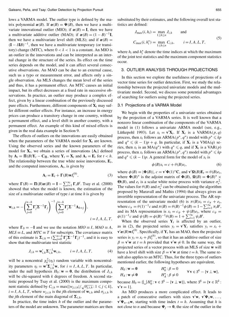
Galeano Pentildea and Tsay Outlier Detection by Projection Pursuit 655
lows a VARMA model The outlier type is defined by the ma-trix polynomial α(B) If α(B) = (B) then we have a multi-variate innovational outlier (MIO) if α(B) = I then we havea multivariate additive outlier (MAO) if α(B) = (1 minus B)minus1Ithen we have a multivariate level shift (MLS) and if α(B) =(I minus δIB)minus1 then we have a multivariate temporary (or transi-tory) change (MTC) where 0 lt δ lt 1 is a constant An MIO isan outlier in the innovations and can be interpreted as an inter-nal change in the structure of the series Its effect on the timeseries depends on the model and it can affect several consec-utive observations An MAO can be due to an external causesuch us a typo or measurement error and affects only a sin-gle observation An MLS changes the mean level of the seriesand thus it has a permanent effect An MTC causes an initialimpact but its effect decreases at a fixed rate in successive ob-servations In practice an outlier may produce a complex ef-fect given by a linear combination of the previously discussedpure effects Furthermore different components of Xt may suf-fer different outlier effects For instance an increase in energyprices can produce a transitory change in one country withouta permanent effect and a level shift in another country with apermanent effect An example of this kind of mixed effects isgiven in the real data example in Section 9
The effects of outliers on the innovations are easily obtainedwhen the parameters of the VARMA model for Xt are knownUsing the observed series and the known parameters of themodel for Xt we obtain a series of innovations At definedby At = (B)Yt minus C where Yt = Xt and At = Et for t lt hThe relationship between the true white noise innovations Etand the computed innovations At is given by
At = Et + (B)wI(h)t (3)
where (B) = (B)α(B) = I minus suminfini=1 iBi Tsay et al (2000)
showed that when the model is known the estimation of thesize of a multivariate outlier of type i at time h is given by
wih = minus(
nminushsum
j=0
primej
minus1j
)minus1(nminushsum
j=0
primej
minus1Ah+j
)
i = IALT
where 0 = minusI and we use the notation MIO equiv I MAO equiv AMLS equiv L and MTC equiv T for subscripts The covariance matrixof this estimate is ih = (
sumnminushj=0 prime
jminus1j)
minus1 and it is easy toshow that the multivariate test statistic
Jih = wprimeih
minus1ih wih i = IALT (4)
will be a noncentral χ2k (ηi) random variable with noncentral-
ity parameters ηi = wprimeminus1ih w for i = IALT In particular
under the null hypothesis H0 w = 0 the distribution of Jih
will be chi-squared with k degrees of freedom A second sta-tistic proposed by Tsay et al (2000) is the maximum compo-nent statistic defined by Cih = max|wjih|radicσjih 1 j ki = IALT where wjih is the jth element of wih and σjih isthe jth element of the main diagonal of ih
In practice the time index h of the outlier and the parame-ters of the model are unknown The parameter matrices are then
substituted by their estimates and the following overall test sta-tistics are defined
Jmax(ihi) = max1lehlen
Jih and
(5)Cmax(ihlowast
i ) = max1lehlen
Cih i = IALT
where hi and hlowasti denote the time indices at which the maximum
of the joint test statistics and the maximum component statisticsoccur
3 OUTLIER ANALYSIS THROUGH PROJECTIONS
In this section we explore the usefulness of projections of avector time series for outlier detection First we study the rela-tionship between the projected univariate models and the mul-tivariate model Second we discuss some potential advantagesof searching for outliers using the projected series
31 Projections of a VARMA Model
We begin with the properties of a univariate series obtainedby the projection of a VARMA series It is well known that anonzero linear combination of the components of the VARMAmodel in (1) follows a univariate ARMA model (see egLuumltkepohl 1993) Let xt = vprimeXt If Xt is a VARMA(pq)
process then xt follows an ARMA(plowastqlowast) model with plowast kpand qlowast (k minus 1)p + q In particular if Xt is a VMA(q) se-ries then xt is an MA(qlowast) with qlowast q and if Xt is a VAR(p)
process then xt follows an ARMA(plowastqlowast) model with plowast kpand qlowast (k minus 1)p A general form for the model of xt is
φ(B)xt = c + θ(B)et (6)
where φ(B) = |(B)| c = vprime(1)lowastC and vprime(B)Et = θ(B)et where (B)lowast is the adjoint matrix of (B) (B) = (B)lowast times(B) and et is a scalar white noise process with variance σ 2
e The values for θ(B) and σ 2
e can be obtained using the algorithmproposed by Maravall and Mathis (1994) that always gives aninvertible representation of the univariate process The AR rep-resentation of the univariate model (6) is π(B)xt = cπ + etwhere cπ = θ(1)minus1c and π(B) = θ(B)minus1φ(B) = 1minussuminfin
i=1 πiBiand its MA representation is xt = cψ + ψ(B)et where cψ =φ(1)minus1c and ψ(B) = φ(B)minus1θ(B) = 1 + suminfin
i=1 ψiBiWhen the observed series Yt is affected by an outlier
as in (2) the projected series yt = vprimeYt satisfies yt = xt +vprimeα(B)wI(h)
t Specifically if Yt has an MAO then the projectedseries is yt = xt + βI(h)
t so that it has an additive outlier of sizeβ = vprimew at t = h provided that vprimew = 0 In the same way theprojected series of a vector process with an MLS of size w willhave a level shift with size β = vprimew at time t = h The same re-sult also applies to an MTC Thus for the three types of outliersmentioned earlier the following hypotheses are equivalent
H0 w = 0
HA w = 0hArr Hlowast
0 β = 0
HlowastA β = 0
forallv isin Sk minus v perp w
because H0 = ⋃Hlowast0 v isin Sk minus v perp w where Sk = v isin R
k vprimev = 1
An MIO produces a more complicated effect It leads toa patch of consecutive outliers with sizes vprimew vprime1w
vprimenminushw starting with time index t = h Assuming that h isnot close to n and because j rarr 0 the size of the outlier in the
656 Journal of the American Statistical Association June 2006
patch tends to 0 In the particular case where vprime iw = ψivprimewforall i = 1 n minus h yt has an innovational outlier at t = h withsize β = vprimew But if vprime iw = 0 i = 1 n minus h then yt hasan additive outlier at t = h with size w and if vprime iw = vprimewi = 0 n minus h then yt has a level shift at t = h with sizeβ = vprimew Therefore the univariate series yt obtained by the pro-jection can be affected by an additive outlier a patch of outliersor a level shift
32 Some Advantages of Projection Methods
The first advantage of using projections to search multivari-ate outliers is simplicity By using univariate series we do notneed to prespecify a multivariate model for the underlying se-ries in outlier detection Second if the model parameters areknown then a convenient projection direction will lead to teststatistics that are more powerful than the multivariate onesThird as we show later in a Monte Carlo study the same con-clusion continues to hold when the parameters are estimatedfrom the observed series
To illustrate the second advantage consider a k-dimensionaltime series Yt generated from the VARMA model in (1) andaffected by an MAO MLS or MTC at t = h Let V be a k times kmatrix such that the first column is ww and the remainingcolumns consist of k minus 1 vectors that are orthogonal to w andhave unit length The multivariate series VprimeYt is affected by anoutlier of size (w0 0)prime at time t = h Note that the out-lier affects only the first component of the transformed seriesBecause the multivariate test statistic Jih of (4) is invariant tolinear transformations its value is the same for both Yt andVprimeYt series Thus all of the information concerning the outlieris in the first component of VprimeYt which is the projection of thevector time series in the direction of the outlier The remain-ing components of VprimeYt are irrelevant for detecting the out-lier Moreover because the test statistic Jih is distributed as a
noncentral χ2k (ηi) with noncentrality parameter ηi = wprimeminus1
ih wits power is given by Pow(M) = Pr(Jih gt χ2
kα) where χ2kα
is the 100αth percentile of the chi-squared distribution withk degrees of freedom In contrast projecting the series Yt ona given direction v we obtain a series yt affected by an out-lier at time t = h and the univariate test statistic jih = β2
ihσ2ih
where βih is a consistent estimate of β is distributed as a non-central χ2
1 (νi) with noncentrality parameter νi = β2σ 2ih where
β = vprimew and σ 2ih = var(βih) The power of this test statistic
is Pow(U) = Pr( jih gt χ21α) Because the detection procedure
that we propose is affine equivariant for simplicity we assumethat Yt = Et is white noise and that = I If v = ww thenit is easy to see that for every w ηi = νi = wprimew for i = I AηL = νL = (nminush+1)wprimew and ηT = νT = (1minusδ2(nminush+1))(1minusδ2)wprimew The powers Pow(U) and Pow(M) and their differ-ences Pow(U) minus Pow(M) for the case of an MAO are shownin Figure 1 for different values of wprimew The figure shows thatthe larger the number of components the larger the advantageof the projection test over the multivariate one When the sizeof the outlier increases both tests have power close to 1 andhence the difference goes to 0 for large outliers In Section 8we show by a simulation study that for correlated series thesame conclusion will continue to hold when the parameters areestimated from the data although the power will depend on themodel
4 FINDING THE PROJECTION DIRECTIONS
The objective of projection pursuit algorithms is to find in-teresting features of high-dimensional data in low-dimensionalspaces via projections obtained by maximizing or minimizingan objective function termed the projection index which de-pends on the data and the projection vector It is commonly
(a)
(b)
Figure 1 Powers of the Multivariate and the Projection Statistics as a Function of the Outlier Size (a) Absolute powers (b) difference of powers
Galeano Pentildea and Tsay Outlier Detection by Projection Pursuit 657
assumed that the most interesting projections are the farthestones from normality showing some unexpected structure suchas clusters outliers or nonlinear relationships among the vari-ables General reviews of projection pursuit techniques havebeen given by Huber (1985) Jones and Sibson (1987) andPosse (1995) Pentildea and Prieto (2001a) proposed a procedurefor multivariate outlier detection based on projections that max-imize or minimize the kurtosis coefficient of the projected dataPentildea and Prieto (2001b) showed that these projected directionsare also useful to identify clusters in multivariate data PanFung and Fang (2000) suggested using projection pursuit tech-niques to detect high-dimensional outliers and showed that theprojected outlier identifier is a centered Gaussian process on ahigh-dimensional unit sphere Pan and Fang (2002) suggestedlooking for outliers in the projection directions given by the di-rections that maximizes the sample kurtosis and skewness
In this section we generalize the application of projectionsto multivariate time series analysis and define a maximum dis-crimination direction as the direction that maximizes the size ofthe univariate outlier vprimew with respect to the variance of theprojected series We show that for an MAO MLS and MTCthe direction of the outlier is a direction of maximum discrimi-nation which can be obtained by finding the extremes of thekurtosis coefficient of the projected series For an MIO weprove that the direction of the outlier is a maximum discrimina-tion direction for the innovations series which can be obtainedby projecting the innovations
In what follows for a time series zt we define z = 1n
sumnt=1 zt
and zt = zt minus z where n is the sample size Let Yt and At bethe observed series and innovations in (2) and (3) For easein presentation and without loss of generality we assume thatE(Xt) = 0 and X = cov(Xt) = I and define the determinis-tic variable Rt = α(B)wI(h)
t Projecting Yt on the direction vwe obtain yt = xt + rt where rt = vprimeRt In addition we haveE[ 1
n
sumnt=1 Yt] = E(Y) = R and
Y = E
[1
n
nsum
t=1
(Yt minus Y)(Yt minus Y)prime]
= E
[1
n
nsum
t=1
YtYprimet
]
= I + R
where R = 1n
sumnt=1 RtRprime
t Using the results of Rao (1973p 60) the maximum of (vprimew)2(vprimeYv) under the constraintvprimeYv = 1 is v = Yw For the cases of MAO MLS andMTC we have Y = I + βiwwprime with βi given by
βA = n minus 1
n2
βL = n minus h + 1
n
(h minus 1
n
)
βT = 1
n
[(1 minus δ2(nminush+1)
1 minus δ2
)
minus 1
n
(1 minus δ(nminush+1)
1 minus δ
)2]
and v = (1 + βiwprimew)w Thus the interesting direction v of pro-jection is proportional to w The same result also holds in theMIO case for the maximum of (vprimew)2(vprimeAv) under the con-straint vprimeAv = 1 where A is the expected value of the co-variance matrix of the innovations At
We prove next that the direction of the outlier w can befound by maximizing or minimizing the kurtosis coefficient of
the projected series Toward this end we need some preliminaryresults the proofs of which are given in the Appendix
Lemma 1 The kurtosis coefficient γy(v) of the project seriesyt = vprimeYt under the restriction vprimeYv = 1 is
γy(v) = 3 minus 3(vprimeRv)2 + ωr(v) (7)
where ωr(v) = 1n
sumnt=1 r4
t
Lemma 2 The extreme directions of the kurtosis coefficientof yt under the constraint vprimeYv = 1 are given by the eigen-vectors of the matrix
sumnt=1 βt(v)RtRprime
t associated with eigen-values micro(v) = n(vprimeRv)2(γr(v) minus 3) where βt(v) = (vprimeRt)
2 minus3(vprimeRv) minus micro(v)n and γr(v) is the kurtosis coefficient ofrt = vprimeRt Moreover the directions that maximize or minimizethe kurtosis coefficient are given by the eigenvectors associatedwith the largest and the smallest eigenvalues micro(v)
The following theorem shows the usefulness of the extremedirections of the kurtosis coefficient of yt
Theorem 1 Suppose that Xt is a stationary VARMA( pq)process and Yt = Xt + α(B)wI(h)
t as in (2) then we have thefollowing results
a For an MAO the kurtosis coefficient of yt is maximizedwhen v is proportional to w and is minimized when v is orthog-onal to w
b For an MTC the kurtosis coefficient of yt is maximizedor minimized when v is proportional to w and is minimized ormaximized when v is orthogonal to w
c For an MLS the kurtosis coefficient of yt is minimizedwhen v is proportional to w and is maximized when v is or-thogonal to w if
h isin(
1 + 1
2
(
1 minus 1radic3
)
n1 + 1
2
(
1 + 1radic3
)
n
)
Otherwise the kurtosis coefficient of yt is maximized when v isproportional to w and is minimized when v is orthogonal to w
Theorem 1 has two important implications First for anMAO MLS or MTC one of the directions obtained by max-imizing or minimizing the kurtosis coefficient is the directionof the outlier Second these directions are obtained without theinformation of the time index at which the outlier occurs Giventhe characteristics of innovational outliers it is natural to thinkthat the direction of the outlier can be obtained by focusing onthe innovations series This is indeed the case
Corollary 1 If Xt is a stationary VARMA( pq) process andYt = Xt + (B)wI(h)
t as in (2) with At = Et + wI(h)t then the
kurtosis coefficient of at = vprimeAt is maximized when v is pro-portional to w and is minimized when v is orthogonal to w
5 MASKING AND SWAMPING EFFECTS
In the presence of multiple outliers it would be of limitedvalue if one considered only the projections that maximize orminimize the kurtosis coefficient because of the potential prob-lem of masking effects For instance a projection might effec-tively reveal one outlier but almost eliminate the effects of otheroutliers To overcome such a difficulty we present an iterative
658 Journal of the American Statistical Association June 2006
procedure for analyzing a set of 2k orthogonal directions con-sisting of (a) the direction that maximizes the kurtosis coeffi-cient (b) the direction that minimizes the kurtosis coefficientand (c) two sets of k minus 1 directions orthogonal to (a) and (b)Our motivation for using these orthogonal directions is twofoldFirst the results of Section 4 reveal that in some cases the di-rections of interest are orthogonal to those that maximize orminimize the kurtosis coefficient of the projected series sec-ond these directions ensure nonoverlapping information sothat if the effect of an outlier is almost hidden in one directionthen it may be revealed by one of the orthogonal directionsFurthermore after removing the effects of outliers detected inthe original set of 2k orthogonal directions we propose to iter-ate the analysis using new directions until no more outliers aredetected Therefore if a set of outliers are masked in one direc-tion then they may be revealed either in one of the orthogonaldirections or in a later iteration after removing detected outliersTo illustrate we analyze in detail the cases of a series with twoMAOs and an MAO and an MLS
Theorem 2 Suppose that Xt is a stationary VARMA( pq)process Yt is the observed vector series and yt = vprimeYt is a pro-jected scalar series
a Let Yt = Xt +w1I(h1)t +w2I(h2)
t with h1 lt h2 There arethree possibilities as follows
1 If w1 and w2 are proportional to each other then the kur-tosis coefficient of yt is maximized when v is proportionalto wi and is minimized when v is orthogonal to wi
2 If w1 and w2 are orthogonal then the kurtosis coefficientis maximized when v is proportional to the outlier withlarger Euclidean norm and minimized when v is in one ofthe orthogonal directions
3 Let ϕ be the angle between w1 and w2 then the kur-tosis coefficient is approximately maximized when v isthe direction of the outlier that gives the maximum ofw1w2 cosϕw2w1 cosϕ where the quan-tity denotes the ratio between the norm of outlier wi andthe length of the projection of outlier wj on wi wherej = i
b Let Yt = Xt + w1I(h1)t + w2S(h2)
t with h1 lt h2 Then thekurtosis coefficient of yt is maximized or minimized when v isproportional to w2 and it is minimized or maximized when v isorthogonal to w2
In the case of two MAOs Theorem 2 shows that if both out-liers are proportional then the maximum of the kurtosis co-efficient is obtained in the direction of the outliers and if theoutliers are orthogonal then the maximum of the kurtosis is ob-tained in the direction of the outlier with larger Euclidean normand the minimum is obtained in an orthogonal direction Thusan orthogonal direction of the one that gives the maximum ofthe kurtosis coefficient will reveal the presence of the outlierwith smaller norm If the outliers are neither proportional nororthogonal to each other then the direction of the outlier withthe largest projection on the direction of the other outlier willproduce a maximum kurtosis coefficient Note that the projec-tion of w2 on the direction of w1 is given by w2 cosϕ Theratio w1w2 cosϕ is large if w1 is large enough com-pared with w2 in which case the kurtosis coefficient will be
maximized in the direction of w1 or if cosϕ is small enoughin which case an orthogonal direction to w1 will reveal w2
Second the direction of the MLS gives the maximum orthe minimum of the kurtosis coefficient of the projected seriesThus the MLS will be revealed in the directions that maximizeor minimize the kurtosis coefficient of yt Projecting in the or-thogonal directions will eliminate the effect of this level shiftand reveal the second outlier If the statistics for this secondoutlier are not significant then we remove the effect of the levelshift and a new set of directions may reveal the second outlier
In contrast outlier detection procedures are sometimes af-fected by swamping effects that is one outlier affects the seriesin such a way that other ldquogoodrdquo data points appear like outliersThe procedure that we propose in the next section includes sev-eral steps to avoid swamping effects which can appear in theunivariate searches using the projection statistics The idea isto delete nonsignificant outliers after a joint estimation of theparameters and detected outliers We clarified this in the nextsection
6 ALGORITHMS FOR OUTLIER DETECTION
Here we propose a sequential procedure for outlier detectionbased on the directions that mimimize and maximize the kur-tosis coefficient of the projections We refer to these directionsas the optimal projections The procedure is divided into foursteps (1) Obtain these directions (2) search for outliers in theprojected univariate time series (3) remove the effect of all de-tected outliers by using an approximated multivariate modeland (4) iterate the previous steps applied to the cleaned seriesuntil no more outliers are found Note that in step 2 the detec-tion is carried out in two stages First MLSs are identified andsecond MIOs MAOs and MTCs are found Finally a vectormodel is identified for the cleaned time series and the outliereffects and model parameters are jointly estimated The fittedmodel is refined if necessary for example removing insignifi-cant outliers if any
61 Computation of the Projection Directions
We use the procedure of Pentildea and Prieto (2001b) to constructthe 2k projection directions of interest For an observed vectorseries Yt our goal here is to obtain the maximum and mini-mum of the kurtosis coefficient of the projected series and theorthogonal directions of the optimal projections Toward thisend consider the following procedure
1 Let m = 1 and Z(m)t = Yt
2 Let (m)Z = 1
n
sumnt=1 Z(m)
t Z(m)primet and find vm such that
vm = arg maxvprime
m(m)Z vm=1
1
n
nsum
t=1
(vprime
mZ(m)t
)4 (8)
3 If m = k then stop otherwise define Z(m+1)t = (I minus
vmvprimem
(m)Z )Z(m)
t that is Z(m+1)t is the projection of
the observations in an orthogonal direction to vm Letm = m + 1 and go to step 2
4 Repeat the same procedure to minimize the objectivefunction in (8) to obtain another set of k directionsnamely vk+1 v2k
Galeano Pentildea and Tsay Outlier Detection by Projection Pursuit 659
A key step of the foregoing algorithm is to solve theoptimization problem in (8) Toward this end we use amodified Newton method to solve the system given by thefirst-order optimality conditions nablaγz(v) minus 2λ
(m)Z v = 0 and
vprime(m)Z v minus 1 = 0 by means of linear approximations (See Pentildea
and Prieto 2001b for technical details of the method) One rel-evant issue is that the proposed procedure is affine equivariantthat is the method selects equivalent directions for series mod-ified by an affine transformation
62 Searching for Univariate Outliers
The most commonly used tests for outlier detection in uni-variate time series are the likelihood ratio test (LRT) statis-tics λih i = IALT (see Chang and Tiao 1983 Tsay 1988)Because the location of the outlier and the parameters of themodel are unknown the estimated parameters are used to de-fine the overall test statistics (ihi) = max|λit|1 le t le ni = IALT Using these statistics Chang and Tiao (1983)proposed an iterative algorithm for detecting innovational andadditive outliers Tsay (1988) generalized the algorithm to de-tect level shifts and transitory changes (see Chen and Liu 1993Saacutenchez and Pentildea 2003 for additional extensions)
In this article we consider a different approach There is sub-stantial evidence that using the same critical values for all theLRT statistics can easily misidentify a level shift as an innova-tive outlier (see Balke 1993 Saacutenchez and Pentildea 2003) The latterauthors showed that the critical values for the LRT statistic fordetecting level shifts are different from those for testing addi-tive or innovative outliers Therefore we propose to identify thelevel shifts in a series before checking for other types of outlierToward this end it is necessary to develop a procedure that iscapable of detecting level shifts in the presence of the othertypes of outliers Using the notation of Section 31 Bai (1994)proposed the cusum statistic
Ct = tradicnψ(1)σe
(1
t
tsum
i=1
yi minus y
)
(9)
to test for a level shift at t = h+1 in a linear process and showedthat the statistic converges weakly to a standard Brownianbridge on [01] In practice the quantity ψ(1)σe is replacedby a consistent estimator
ψ(1)σe =[
γ (0) + 2Ksum
i=1
(
1 minus |i|K
)
γ (i)
]12
where γ (i) = cov( yt ytminusi) and K is a quantity such thatK rarr infin and Kn rarr 0 as n rarr infin Under the assumption ofno level shifts in the sample the statistic max1letlen |Ct| is as-ymptotically distributed as the supremum of the absolute valueof a Brownian bridge with cumulative distribution functionF(x) = 1 + 2
suminfini=1(minus1)ieminus2i2x2
for x gt 0 The cusum statis-tic (9) has several advantages over the LRT statistic for detect-ing level shifts First it is not necessary to specify the orderof the ARMA model which can be difficult in the presence oflevel shifts Second as shown in Section 8 this statistic seemsto be more powerful than the LRT in all the models consideredThird the statistic (9) seems to be robust to the presence ofother outliers whereas the LRT statistic is not
621 Level Shift Detection Given the 2k projected uni-variate series yti = vprime
iYt for i = 1 2k we propose an it-erative procedure to identify level shifts based on the algorithmproposed by Inclaacuten and Tiao (1994) and Carnero Pentildea andRuiz (2003) for detecting variance changes and level shifts in awhite noise series Let H be the prespecified minimum distancebetween two level shifts The proposed algorithm divides theseries into pieces after detecting a level shift and proceeds asfollows
1 Let t1 = 1 and t2 = n Obtain
DL = max1leile2k
maxt1letlet2
|Cit| (10)
where Cit is the statistic (9) applied to the ith projected
series for i = 1 2k Let
(imax tmax) = arg max1leile2k
arg maxt1letlet2
|Cit| (11)
If DL gt DLα where DLα is the critical value for thesignificance level α then there is a possible level shift att = tmax + 1 and we go to step 2a If DL lt DLα thenthere is no level shift in the series and the algorithmstops
2a Define t2 = tmax of step 1 and obtain new values of DLand (imax tmax) of (10) and (11) If DL gt DLα and t2 minustmax gt H then we redefine t2 = tmax and repeat step 2auntil DL lt DLα or t2 minus tmax le H Define tfirst = t2 wheret2 is the last time index that attains the maximum of thecusum statistic that is larger than DLα and satisfies t2 minustmax gt H The point tfirst + 1 is the first time point with apossible level shift
2b Define t1 = tmax of step 1 and t2 = n and obtain new val-ues of DL and (imax tmax) of (10) and (11) If DL gt DLα
and tmax minus t1 gt H then we redefine t1 = tmax and re-peat step 2b until DL lt DLα or tmax minus t1 le H Definetlast = t1 where t1 is the last time index that attains themaximum of the cusum statistics that is larger than DLα
and satisfies tmax minus t1 gt H The point tlast + 1 is the lasttime point with a possible level shift
2c If tlast minus tfirst lt H then there is just a level shift and thealgorithm stops If not then keep both values as possi-ble changepoints and repeat steps 2a and 2b for t1 = tfirstand t2 = tlast until no more possible changepoints are de-tected Then go to step 3
3 Define a vector hL = (hL0 hL
rL+1) where hL0 = 1
hLrL+1 = n and hL
1 lt middot middot middot lt hLrL
are the changepoints de-tected in step 2 Obtain the statistic DL in each subin-terval (hL
i hLi+2) and check its statistical significance If
it is not significant then eliminate the correspondingpossible changepoint Repeat step 3 until the number ofpossible changepoints remains unchanged and the timeindexes of changepoints are the same between iterationsRemoving hL
0 = 1 and hLrL+1
= n from the final vector oftime indexes we obtain rL level shifts in the series attime indexes hL
i + 1 for i = 1 L4 Let hL
1 hLrL
be the time indexes of rL detected levelshifts To remove the impacts of level shifts we fit themodel
(I minus 1B minus middot middot middot minus pBp)Ylowastt = Alowast
t (12)
660 Journal of the American Statistical Association June 2006
where Ylowastt = Yt minussumrL
i=1 wiS(hL
i )t and the order p is chosen
such that
p = arg max0leplepmax
AIC(p) = arg max0leplepmax
log |p| + 2k2p
n
where p = 1nminus2pminus1
sumnt=p+1 Alowast
t Alowastprimet and pmax is a pre-
specified upper bound If some of the effects of levelshifts are not significant then we remove the least sig-nificant one from the model in (12) and reestimate theeffects of the remaining rL minus 1 level shifts This processis repeated until all of the level shifts are significant
Some comments on the proposed procedure are in orderFirst the statistic DL is the maximum of dependent randomvariables and has an intractable distribution We obtain criti-cal values by simulation in the next section Second the teststatistics (9) are highly correlated for close observations Thusconsecutive large values of Ct might be caused by a single levelshift To avoid overdetection we do not allow two level shiftsto be too close by using the number H in steps 2 and 3 In thesimulations and real data example we chose H = 10 and foundthat it works well
622 An Algorithm for Outlier Detection Using the level-shift adjusted series we use the following procedure to detectadditive outliers transitory changes and innovative outliers inthe 2k projected univariate series yti = vprime
iYlowastt and their associ-
ated innovational series ati = vprimeiA
lowastt for i = 1 2k
1 For each projected series yti fit an AR( p) with p selectedby the Akaike information criterion (AIC) and computethe LRT statistics λi
At and λiTt In addition compute the
LRT statistics λiIt using the associated innovational se-
ries ati This leads to the maximum statistics
A = max1leile2k
max1letlen
|λiAt|
T = max1leile2k
max1letlen
|λiTt| and (13)
I = max1leile2k
max1letlen
|λiIt|
2 For i = AT and I let Aα Tα and Iα be the crit-ical values for a predetermined significance level α Ifi lt iα for i = IAT then no outliers are found andthe algorithm stops If i gt iα for only one i then iden-tify an outlier of type i and remove its effect using themultivariate parameter estimates If i gt iα for morethan one i then identify the outlier based on the most sig-nificant test statistic and remove its effect using the multi-variate parameter estimates Repeat steps 1 and 2 until nomore outliers are detected
3 Let hA1 hA
rA hT
1 hTrT
and hI1 hI
rI be the
time indexes of the rA rT and rI detected additive out-liers transitory changes and innovative outliers Estimatejointly the model parameters and the detected outliers forthe series Ylowast
t (I minus 1B minus middot middot middot minus pBp)Ylowastlowastt = Alowastlowast
t where
Ylowastlowastt = Ylowast
t minusrAsum
iA=1
wiA I(hA
iA)
t minusrTsum
iT=1
wiT
1 minus δBI(hT
iT)
t
and
Alowastlowastt = Alowast
t minusrIsum
iI=1
wiI I(hI
iI)
t
If some of the outlier effects become insignificant thenremove the least significant outlier and reestimate themodel Repeat this process until all of the remaining out-liers are significant
In Section 8 we obtain critical values for the test statis-tics λi
At λiTt and λi
It through simulation
63 Final Joint Estimation of ParametersLevel Shifts and Outliers
Finally we perform a joint estimation of the model parame-ters the level shifts and the outliers detected using the equation(I minus 1B minus middot middot middot minus pBp)Zt = Dt where
Zt = Yt minusrLsum
iL=1
wiL S(hL
iL)
t minusrAsum
iA=1
wiA I(hA
iA)
t minusrTsum
iT=1
wiT
1 minus δBI(hT
iT)
t
and
Dt = At minusrIsum
iI=1
wiI I(hI
iI)
t
and hL1 hL
rL hA
1 hArA
hT1 hT
rT and hI
1 hIrI
are the time indexes of the rL rA rT and rI detected level shiftsadditive outliers transitory changes and innovative outliers Ifsome effect is found to be not significant at a given level thenwe remove the least significant one and repeat the joint estima-tion until all of the effects are significant
Some comments on the proposed procedure are as followsFirst as mentioned in Section 2 an outlier can be a combina-tion of different effects This does not cause any problem forthe proposed procedure because it allows for multiple outlierdetections at a given time point either in different projectiondirections or in successive iterations The real data example ofSection 9 demonstrates how the proposed procedure handlessuch a situation Second the procedure includes several stepsto avoid swamping effects Specifically after detecting levelshifts we fit an autoregression and remove any nonsignificantlevel shifts We repeat the same step after detecting the othertypes of outlier Finally we perform a joint estimation of modelparameters and detected level shifts and outliers to remove anynonsignificant identification of level shift or outliers
7 THE NONSTATIONARY CASE
In this section we study the case when the time series isunit-root nonstationary Assume that Xt sim I(d1 dk) wherethe dirsquos are nonnegative integers denoting the degrees of dif-ferencing of the components of Xt Let d = max(d1 dk)
and consider first the case of d = 1 which we denote simplyby Xt sim I(1) For such a series in addition to the outliers in-troduced by Tsay et al (2000) we also entertain the multi-variate ramp shift (MRS) defined as Yt = Xt + wR(h)
t whereR(h)
t = (I minus B)minus1S(h)t with S(h)
t being a step function at the timeindex h (ie S(h)
t = 1 if t ge h and = 0 otherwise) This out-lier implies a slope change in the multivariate series and it may
Galeano Pentildea and Tsay Outlier Detection by Projection Pursuit 661
occur in an I(1) series It is not considered in the stationarycase because the series has no time slope Consequently for anMRS we assume that it applies only to the components of Ytwith dj = 1 that is the size of the outlier w = (w1 wk)
primesatisfies wj = 0 if dj = 0
The series Xt can be transformed into stationarity by tak-ing the first difference of its components even though dj mightbe zero for some j As we show later this is not a drawbackfor our method The first differencing affects the existing out-liers as follows In the MIO case (I minus B)Yt = (I minus B)Xt +(B)wI(h)
t where (B) = (I minus B)(B) Therefore an MIOproduces an MIO in the differenced series In the MAO case(I minus B)Yt = (I minus B)Xt + w(I(h)
t minus I(h)tminus1) producing two consec-
utive MAOs with the same size but opposite signs In the MLScase (IminusB)Yt = (IminusB)Xt +wI(h)
t resulting in an MAO of thesame size In the MTC case (IminusB)Yt = (IminusB)Xt +ζ(B)wI(h)
t where ζ(B) = 1 + ζ1B + ζ2B2 + middot middot middot such that ζj = δjminus1(1 minus δ)Thus an MTC produces an MTC with decreasing coefficients ζj
In the MRS case (I minus B)Yt = (I minus B)Xt + wS(h)t which pro-
duces an MLS with same sizeThe results of Section 4 can be extended to include the
aforementioned outliers induced by differencing For instanceTheorem 1 shows that the directions that maximize or minimizethe kurtosis coefficient of the projected series under the pres-ence of two consecutive MAOs with the same size but oppositesigns are the direction of the outlier or a direction orthogonal toit Therefore in the I(1) case we propose a procedure similarto that of the stationary case for the first differenced series Thisprocedure consists of the following steps
1 Take the first difference of all of the components of YtCheck for MLS as in Section 621 All of the level shiftsdetected in the differenced series are incorporated as rampshifts in the original series and are estimated jointly withthe model parameters If any ramp shift is not significantthen remove it from the model and repeat the detectingprocess until all of the ramp shifts are significant Thisleads to a series Ylowast
t = Yt minus sumrRi=1 wiR
(h)t that is free of
ramp shifts2 Take the first difference of all of the components of Ylowast
t The series (I minus B)Ylowast
t may be affected by MIOs two con-secutive MAOs MAOs and MTCs Then proceed as inSection 622 All of the outliers detected in the differ-enced series are incorporated by the corresponding effectsin the original series and are estimated jointly with themodel parameters If any of the outliers becomes insignif-icant then remove it from the model Repeat the processuntil all of the outliers are statistically significant
The procedure can also be applied to series that have dj = 0for some components and to cointegrated series In thesecases nablaYt is overdifferenced implying that its MA componentcontains some unit roots Nevertheless this is not a problem forthe proposed procedure If the series is not cointegrated thenany projection direction provides an univariate series withoutunit roots in its MA component If the series is cointegratedthen the directions of the outliers will in general be differentfrom the directions of cointegration In other words if v is avector obtained by maximizing or minimizing the kurtosis co-efficient then it is unlikely to be a cointegration vector and
vprimenablaYt = nabla(vprimeYt) is stationary and invertible because vprimeYt isa nonstationary series However if the series are cointegratedthen the final estimation should be carried out using the errorcorrection model of Engle and Granger (1987) Note that if v isthe cointegration vector then vprimeYt is stationary and nablavprimeYt isoverdifferenced Although no relationship is expected betweenthe outlier directions and the cointegration vector we have ver-ified by using Monte Carlo simulations that the probabilityof finding the cointegration relationship as a solution of theoptimization algorithm is very low Specifically we generated10000 series from a vector AR(1) model with two componentsand a cointegration relationship and found the directions in (8)To compare the directions with the cointegration vector wecalculated the absolute value of the cosine of the angle be-tween these two directions The average value of this cosineis 62 with variance 09 It is easy to show that if the angle hasa uniform distribution in the interval (0π) then the distribu-tion of the cosine of the angle has mean 63 and variance 09Next we repeated the same experiment with the same seriesbut affected by outliers level shifts or transitory changes andobtained in every case that the mean of the angles between thedirection found and the cointegrating direction is the one thatexits between the direction of the outlier and the cointegrationdirection Therefore we conclude that there should be no con-fusion between the cointegration vectors and the directions thatmaximize or minimize the kurtosis coefficient of the projectedseries
Consider next the case where d = 2 Define a multivari-ate quadratic shift (MQS) as Yt = Xt + wQ(h)
t where Q(h)t =
(I minus B)minus1R(h)t This outlier introduces a change in the quadratic
trend of the multivariate series The series Xt can be trans-formed into a stationary one by taking the second differencesHence an MQS is transformed into an MLS an MRS is trans-formed into an MAO and so on A similar procedure as thatproposed for the I(1) case applies In fact the discussion canbe generalized to handle outliers in a general I(d) series
8 SIMULATIONS AND COMPUTATIONAL RESULTS
In this section we investigate the computational aspects of theproposed procedures through simulation First we obtain criti-cal values for all of the test statistics second we compare thepower of the multivariate and projection procedures for detect-ing outliers We begin with the power of detecting level shiftsfollowed by power of identifying other types of outlier To savespace we show only the results for the stationary case
81 Critical Values
Critical values of the test statistics for outlier detection forunivariate and multivariate time series are usually obtainedthrough simulation using a numerous series from different mod-els For instance the outlier detection routines in the pro-grams TRAMO and SCA use critical values obtained by sucha simulation study We follow this stream and consider eightVARMA( pq) models to generate the critical values The di-mensions used in the simulation are k = 235 and 10 and theparameter matrices used are given in Table 1 The constant termof the models is always the vector 1k and the innovations co-variance matrix is the identity matrix For cases of k = 2 and 3the AR parameter matrices have eigenvalues of approximately
662 Journal of the American Statistical Association June 2006
Table 1 Vector Time Series Models Used in Simulation Study
Model
1 2 3
Dimension k = 2
[6 22 4
] [6 22 4
]
[minus7 0minus1 minus3
] [minus7 0minus1 minus3
]
Model
4 5 6
Dimension k = 3
[6 2 02 4 06 2 5
] [6 2 02 4 06 2 5
]
[minus7 0 0minus1 minus3 0minus7 0 minus5
] [minus7 0 0minus1 minus3 0minus7 0 minus5
]
Model 7
Dimension k = 5 diag() = (9 7 5 3 1) and (i i + 1) = minus5 i = 1 4
(i j) = 0 elsewhere
Model 8
Dimension k = 10 diag() = (9 8 1 0) and (i i + 1) = minus5 i = 1 9
(i j) = 0 elsewhere
276 and 724 and 276 5 and 724 whereas the MA para-meter matrices have eigenvalues minus3 and minus7 and minus3minus5and minus7 For the cases where k = 5 and 10 the AR parametermatrices have nonzero elements in their main and first upper di-agonals only and their eigenvalues are the elements of their re-spective main diagonals Using the eight models we generatedcritical values of the test statistics IAL and T in (13)and DL in (10) The LRT statistic for detecting level shifts isincluded for comparison purposes
The sample sizes used are n = 50100200300400and 500 covering most of the cases encountered in practiceFor a given model and sample size we generated 10000 se-ries and computed the test statistics Table 2 summarizes theempirical critical values of the simulation From this table wesee only minor differences in the critical values among dif-ferent models of the same dimension and hence recommendthe critical values in Table 3 for practical use In applicationif the sample size is different from those used in the simula-tion then we recommend interpolating the values of Table 3To better understand the relationship between critical valuesand the number of components and sample size we fitted threelinear regressions in which each column of critical values inTable 3 at the 95th percentile serving as the dependent vari-ables with the number of components k and the number ofobservations n as the regressors The fitted regressions arei = 324 + 1561k + 0014n L = 286 + 0780k + 0008nand DL = 121+ 0240k + 0005n for i = IAT All estimatedparameters are statistically significant and the R2 of the regres-sions are 97 94 and 82 We used these three regressions toobtain critical values for various samples sizes and numbersof components and found that a small increase in the samplesize produced a small increase in the critical values The threeregressions work well in general
Finally we also obtained critical values for the multivariatetest statistics in (5) through the same simulation method forsample sizes n = 100 and 200 Table 4 shows the recommendedcritical values for practical use These critical values are used inpower comparisons of the next section
82 Power and Robustness Comparison of the Statisticsfor Detecting Level Shifts
Next we compare the performance of the multivariate LRTstatistics the test statistics based on projections and the cusumtest for detecting level shifts We use sample sizes n = 100and 200 and three different outlier sizes wL = 3 times 1k 4 times 1kand a random wL The direction of the random wL is generatedby drawing a uniform [01] random variable u for each com-ponent of wL and defining wLi = 0 or 3 if u is in the interval(012) or (121) If wLi = 0 for all i then we discard theoutlier
For a given sample size and level shift we generated 1000series and computed the test statistic Jmax in (5) for a level shiftthe maximum projection statistic L in (13) and the maximumcusum statistic in (10) based on the proposed procedure Wecompare each statistic with its critical values in Tables 3 and 4at the 5 significance level and tabulate the number of times alevel shift is detected The results are given in the first part ofTable 5 (see columns Jmax L and DL) For all of the mod-els considered the cusum test outperforms the other two butall three tests seem to have good power when the sample sizeis 200
We also study the power of these three statistics in the pres-ence of other outliers Specifically for each model we gener-ated 1000 series of size n = 100 Each series is contaminatedby an MIO at hI = 20 with size wI = w times 1k an MAO athA = 40 with size wA = minusw times 1k an MTC at hT = 80 with sizewT = minusw times 1k and an MLS at hL = 60 with size wL = w times 1kwhere w = 3 or 4 A random vector w generated by the samemethod as before is also used as the size for all outliers Wecompute and compare the three test statistics of level shift withtheir respective critical values in Tables 3 and 4 at the 5 sig-nificance level The power of these three statistics are given inthe second part of Table 5 (see columns Jmax L and DL)All three tests are affected by the presence of other outliers butsimilar to the case of a single level shift the cusum test contin-ues to outperform the other two test statistics Furthermore wemeasured the power loss of each test by
loss(i) = 1 minus power with outliers in model i
power with no outliers in model i
and obtained the mean power loss of the three test statistics forthe eight models used with w = 3 The average losses for themultivariate statistic the projection statistic and the cusum testare 241 133 and 54 Therefore the multivariate andprojection test statistics for level shift seem to be more suscep-tible to masking effects than the cusum test statistic
Finally we study the robustness properties of these statisticsin the presence of other outliers With this objective we obtainthe empirical type I error and compare it with the nominal levelof the test We use a generating procedure similar to that of thepower study to conduct the simulation However for each gen-erated series the outliers consist of an MIO at hI = 25 with size
Galeano Pentildea and Tsay Outlier Detection by Projection Pursuit 663
Table 2 Empirical Critical Values of the Test Statistics Considered
95th percentiles 99th percentiles
n k M ΛI ΛA ΛL ΛT DL ΛI ΛA ΛL ΛT DL
50 2 1 353 348 291 347 126 381 375 324 376 1322 347 347 287 334 126 390 376 317 370 1333 357 341 297 344 125 392 384 326 372 132
3 4 390 377 308 370 128 410 394 341 391 1355 385 371 294 365 129 413 394 349 394 1366 389 366 307 370 128 411 391 345 393 135
5 7 420 392 334 377 131 445 424 369 402 136
10 8 492 467 375 430 134 513 489 421 456 139
100 2 1 375 371 308 364 134 408 403 340 406 1442 375 361 306 359 133 415 398 345 398 1433 376 362 308 363 134 412 402 350 406 143
3 4 403 380 319 378 137 439 410 350 415 1455 408 391 316 377 136 445 409 349 414 1456 400 378 316 375 136 436 406 356 410 145
5 7 449 414 347 413 144 477 451 384 449 151
10 8 530 494 382 479 149 559 528 425 510 153
200 2 1 401 392 315 395 141 428 424 354 429 1502 397 388 318 384 140 420 419 350 428 1493 395 384 321 380 140 425 411 349 410 150
3 4 427 405 325 407 143 477 439 369 446 1555 434 409 325 406 142 477 444 358 450 1546 432 398 329 404 142 469 434 371 437 155
5 7 469 432 356 433 154 504 470 394 466 167
10 8 553 513 384 507 162 593 557 427 542 174
300 2 1 405 403 325 400 143 432 431 365 430 1562 407 393 322 401 142 430 427 366 430 1553 404 392 326 398 143 434 434 372 425 156
3 4 438 418 338 411 147 473 450 379 453 1615 438 417 332 417 146 480 461 364 452 1606 436 413 338 417 147 472 450 377 460 160
5 7 482 445 363 448 154 531 479 399 483 170
10 8 562 522 389 511 167 599 560 430 546 181
400 2 1 413 408 341 409 144 450 447 383 447 1582 417 405 342 405 145 462 437 377 450 1573 419 405 338 413 144 464 439 378 460 158
3 4 436 424 345 426 147 489 461 393 470 1625 444 434 354 424 148 479 471 385 465 1616 444 421 348 420 148 486 465 389 452 162
5 7 490 447 360 451 157 538 489 405 488 173
10 8 569 524 392 515 168 603 568 432 553 182
500 2 1 418 419 346 421 145 462 454 384 445 1602 418 413 342 411 146 460 452 382 453 1593 418 407 346 414 145 448 448 382 450 159
3 4 446 428 350 426 149 491 471 396 472 1625 451 432 353 432 148 498 473 391 475 1636 444 431 356 425 149 493 467 391 467 163
5 7 495 453 365 457 159 540 492 410 501 178
10 8 577 525 395 519 169 606 570 435 558 184
NOTE These values are based on sample size n and 10000 realizations M denotes the models in Table 1
wI = w times 1k an MAO at hA = 50 with size wA = minusw times 1k andan MTC at hT = 75 with size wT = w times 1k where w = 3 or 4Again we also used a random vector w generated as beforefor the size of all outliers The last eight rows of Table 5 givethe frequencies that the test statistic is greater than its empiri-cal 95th percentile of Tables 3 and 4 These frequencies denotechances of a false detection of a level shift by the three statis-tics Once again the cusum statistic outperforms the other twoin maintaining the size of a test and being robust to the other
types of outliers The multivariate and projection statistics seemnot robust to the presence of other outliers
83 Power Comparison of the Multivariate andUnivariate Statistics for Other Outliers
In this section we investigate the power of the test statisticsfor detecting other types of outlier The outliers considered areMAOs MIOs and MTCs Again we used the eight models inTable 1 and sample sizes n = 100 and 200 The outlier occurs
664 Journal of the American Statistical Association June 2006
Table 3 Recommended Critical Values of the Test StatisticsConsidered for Sample Size n
95th percentiles 99th percentiles
n k ΛI ΛA ΛT ΛL DL ΛI ΛA ΛT ΛL DL
50 2 35 29 126 38 32 1333 38 30 128 40 34 1355 40 33 131 42 37 136
10 46 37 134 49 42 139
100 2 37 31 134 41 34 1433 39 32 136 42 35 1455 42 34 144 46 39 151
10 50 38 149 53 42 153
200 2 39 32 140 42 36 1503 41 33 142 45 37 1555 44 36 154 48 39 167
10 52 38 162 56 43 174
300 2 40 33 143 43 37 1563 42 34 147 46 38 1605 46 36 154 50 41 170
10 53 39 167 57 43 181
400 2 41 34 144 45 38 1583 43 35 148 47 39 1625 46 36 157 51 42 173
10 54 39 168 58 43 182
500 2 42 34 145 45 38 1593 43 35 149 48 39 1635 47 37 159 51 41 178
10 55 40 169 59 44 184
at t = n2 and assumes three possible sizes as before For eachcombination of model sample size and outlier we generated1000 series to compute the proposed test statistics We thencompared the statistics with their empirical 95th percentiles ofTables 3 and 4 and tabulated the frequencies of detecting a sig-nificant outlier Table 6 summarizes the power of various teststatistics From this table it seems that projection test statis-tics outperform their corresponding multivariate counterpartsOverall our limited simulation study supports the use of pro-jections and cusum statistics in detecting outliers in a vectortime series
9 AN ILLUSTRATIVE EXAMPLE
We illustrate the performance of the proposed proceduresby analyzing a real example The data are the logarithms ofthe annual gross national product (GNP) of Spain Italy andFrance denoted by S I and F from 1947 to 2003 The serieshave 57 observations and are depicted by solid lines in Fig-ure 2 Because the GNP are clearly nonstationary we take thefirst difference of each series We then compute the projection
directions using the proposed procedure of Section 6 and ap-ply the level shift detection algorithm to detect ramp shifts inthe original series The critical value is chosen by means ofthe regressions in Section 81 and turns out to be 132 Thealgorithm detects a ramp shift at time hL
1 = 1975 The valueof the test statistic (10) for the time index is 139 To esti-mate the effect of the ramp shift we first check whether theseries are cointegrated using Johansenrsquos test (Johansen 1991)We find a cointegration vector β and we use the AIC to selectthe error correction model with a cointegrating vector given bynablaYt = D1nablaYtminus1 minus αβ primeYtminus1 + At where the estimated para-meters are
D1 =(
299 095 510
069 344 524
100 221 728
)
α =(
007minus001003
)
and
β =( 10762
minus2235511975
)
Note that this model is equivalent to the VAR(2) modelYt = 1Ytminus1 + 2Ytminus2 + At with 1 = I + D1 minus αβ prime and2 = minusD1 Then using this model we remove the effect ofthe ramp shift by estimating the regression model At = (I minus1B minus 2B2)wR(1975)
t + Et and obtain the series free from theeffect of the ramp shift by Ylowast
t = Yt minus wR(1975)t
Next we consider the detection of other types of outlier Thecritical value is chosen using the fitted regression of Section 81and turns out to be 38 The first part of Table 7 summarizes theresults of the detection procedure It identifies an MLS in 1966and its effect on the series is removed as in the case of the MRSThe procedure then detects an MAO in 1975 which is estimatedand cleaned from the series The procedure fails to detect anyother outliers and is terminated The outlier-adjusted series areshown by dashed lines in Figure 2
After identifying the outliers for the series we estimatejointly the outlier effects and the model parameters using a first-order vector error correction model with a cointegration rela-tionship The estimated effects of the three detected outliersalong with the t-ratios of the estimates are given in Table 8The ramp shift detected by the algorithm in 1975 implies a de-crease in the rate of GNP growth of about 2 in the three coun-tries with the largest in Italy (minus22) and smallest in Spain
Table 4 Empirical Critical Values of the Multivariate Statistics Considered
95th percentiles 99th percentiles
n k Jmax (I) Jmax (A) Jmax (L) Jmax (T) Jmax (I) Jmax (A) Jmax (L) Jmax (T)
100 2 140 135 95 136 161 157 113 1633 160 158 117 154 183 181 136 1845 189 192 144 187 215 223 173 214
10 254 258 192 267 276 287 218 267
200 2 155 159 108 157 185 194 134 1893 178 183 129 180 207 208 159 2035 218 223 166 217 254 256 200 242
10 298 303 217 296 333 345 257 331
Galeano Pentildea and Tsay Outlier Detection by Projection Pursuit 665
Table 5 Empirical Power of Multivariate Projection and Cusum Test Statistics for Detecting a Level Shift
w = 3 times 1k w = 4 times 1k w = random
n k M hI hA hL hT Jmax ΛL DL Jmax ΛL DL Jmax ΛL DL
100 2 1 50 700 830 100 966 982 100 530 829 9922 2 50 583 826 100 892 969 100 526 810 9932 3 50 465 733 876 915 932 100 414 700 8633 4 50 936 927 996 100 988 100 604 710 9843 5 50 681 988 100 947 997 100 275 953 1003 6 50 863 866 887 989 990 992 283 836 8815 7 50 433 981 986 837 998 998 333 750 856
10 8 50 286 938 964 727 969 983 150 802 809
200 2 1 100 807 954 100 981 996 100 743 839 1002 2 100 922 956 100 970 993 100 861 934 1002 3 100 781 906 995 971 984 100 731 872 9723 4 100 987 989 100 100 100 100 922 747 1003 5 100 858 998 100 990 100 100 837 966 1003 6 100 975 978 100 996 997 100 808 958 1005 7 100 709 998 999 947 999 100 735 757 976
10 8 100 694 100 100 973 100 100 532 865 961
100 2 1 20 40 60 80 456 760 926 730 918 993 450 778 9292 2 20 40 60 80 520 876 100 743 967 100 637 874 1002 3 20 40 60 80 170 536 666 403 843 866 356 704 1003 4 20 40 60 80 736 740 903 920 850 100 473 645 9063 5 20 40 60 80 613 816 100 713 920 100 780 915 1003 6 20 40 60 80 636 553 743 870 800 950 256 794 9985 7 20 40 60 80 143 860 874 173 904 939 254 593 847
10 8 20 40 60 80 32 584 746 27 619 798 60 581 716
100 2 1 25 50 75 40 140 33 26 263 33 35 150 452 2 25 50 75 3 90 30 13 110 20 7 80 172 3 25 50 75 40 213 43 23 313 46 9 105 273 4 25 50 75 63 156 30 70 280 63 43 193 413 5 25 50 75 33 80 40 23 126 43 3 90 273 6 25 50 75 163 223 43 166 273 46 19 123 395 7 25 50 75 34 361 45 44 495 55 58 317 48
10 8 25 50 75 46 448 43 39 604 46 45 389 33
NOTE n is the sample size M denotes the model in Table 1 hi denotes time point at which a type i outlier occurs and w is the outlier
Table 6 Empirical Power of Multivariate and Projection Test Statistics for Detecting an Outlier in a Vector Time Series
n = 100 h = 50 n = 200 h = 100
w = 3 times 1k w = 4 times 1k w = random w = 3 times 1k w = 4 times 1k w = random
k M Jmax ΛI Jmax ΛI Jmax ΛI Jmax ΛI Jmax ΛI Jmax ΛI
MIO2 1 599 778 950 980 442 659 588 718 926 968 426 5612 2 539 715 898 953 364 581 585 684 925 955 387 5282 3 511 686 880 952 405 612 570 683 927 956 424 5403 4 819 915 996 992 463 745 816 875 100 100 483 6673 5 620 761 951 974 332 700 674 762 977 985 342 6403 6 618 781 923 976 385 702 671 758 982 988 428 6385 7 954 997 100 100 587 914 967 993 100 100 575 825
10 8 996 100 100 100 697 997 981 100 100 100 804 984
MAO2 1 866 936 993 993 583 863 873 936 993 100 552 7432 2 670 960 960 100 389 876 670 910 956 993 356 7572 3 910 990 996 100 444 877 980 980 100 100 362 6913 4 983 993 996 100 686 849 993 996 100 100 661 6933 5 786 956 986 100 375 863 826 896 990 990 377 7533 6 970 990 996 100 397 912 988 978 100 100 463 8085 7 911 994 100 100 749 935 975 975 100 100 726 848
10 8 992 100 100 100 816 971 100 100 100 100 901 953
MTC2 1 613 886 933 986 461 826 610 886 980 980 418 7832 2 645 970 940 100 588 937 660 920 946 993 621 8712 3 713 936 926 993 577 867 736 903 977 986 608 8183 4 900 980 100 100 594 849 920 928 995 995 549 6813 5 710 976 953 996 670 914 753 933 993 100 617 7733 6 826 956 970 986 524 882 959 957 100 992 539 8155 7 972 996 100 100 694 884 992 100 100 100 711 802
10 8 972 100 100 100 763 974 994 100 100 100 813 947
NOTE n is the sample size M denotes the model in Table 1 h is the time index of outlier and w is the size of the outlier
666 Journal of the American Statistical Association June 2006
(a)
(b)
(c)
Figure 2 Original ( mdashndash) and Modified ( - - - -) Logarithms of the GNP of (a) Spain (b) Italy and (c) France
(minus167) The detected shift can be associated with the firstoil crisis In fact the ramp shift is visible from the plot of theseries The proposed algorithm also identifies an MAO in 1975indicating that the first year of the oil crisis also had a transitoryeffect that was most important in Italy (minus67) As mentionedin Section 6 the proposed procedure allows for multiple outlierdetections at a time point In this case one MRS affecting all ofthe components and one MAO affecting primarily the GNP ofItaly are found The final fitted vector error correction model is
nablaYt =(
2856 1839 3461
0341 6710 2721minus0912 3765 5778
)
nablaYtminus1
minus(
007minus000002
)
(14412 minus21651 8132 )Ytminus1 + At
There are marked changes in the parameter estimates ofthe model with and without outlier detection For instancesubstantial changes in the diagonal elements of the D1 ma-trix are observed before and after the outlier detection for theItalian and French GNP The estimates of the cointegration vec-tor also change The estimated long-run equilibrium relation-ship between the variables before outlier detection is roughly(5S + 5F) minus I After outlier modeling the cointegration vec-tor becomes roughly (64S + 36F) minus I which gives heavierweight to the Spanish GNP
Finally we compare the results with those obtained by ap-plying the procedure of Tsay et al (2000) We obtained criticalvalues for the multivariate test statistics in a simulation not re-ported here using the models in Table 1 The 5 critical valuesfor the multivariate statistics are 173 for MIO MAO and MTCand 148 for MLS The critical values for the component statis-tics are 39 for MIO MAO and MTC and 36 for MLS The
Table 7 Outliers Found by the Proposed Algorithm and the Tsay Pentildea and Pankratz Procedure
Proposed procedureIterations (ΛI hI ) (ΛA hA) (ΛL hL) (ΛT hT ) Time Type
1 (411 1966) (405 1965) (478 1966) (422 1966) 1966 MLS2 (337 1976) (477 1975) (415 1975) (445 1975) 1975 MAO3 (314 1960) (374 1960) (349 1960) (368 1960)
Procedure of Tsay Pentildea and PankratzIterations (JI hI ) (JA hA) (JL hL) (JT hT ) Time Type
1 (1508 1966) (1554 1965) (1139 1975) (1411 1966)
Iterations (CI hI ) (CA hA) (CL hL) (CT hT ) Time Type
2 (378 1966) (384 1965) (316 1975) (342 1966)
Galeano Pentildea and Tsay Outlier Detection by Projection Pursuit 667
Table 8 Estimation of the Sizes of the Outliers Detectedby the Algorithm
S I FTime Type (t-ratio) (t-ratio) (t-ratio)
1966 MLS 0165 0473 0152(17046) (70546) (20114)
1975 MRS minus0167 minus0224 minus0196(minus19723) (minus24668) (minus22817)
1975 MAO minus0434 minus0672 minus0312(minus18392) (minus41121) (minus16917)
second part of Table 7 summarizes the results using the samefirst-order vector error correction model The procedure fails todetect any outliers at the 5 level even though some of the teststatistics are only slightly smaller than the critical values
APPENDIX PROOFS
Proof of Lemma 1
Taking into account that yt = xt + rt xt and rt are independent thatE[xt] = E[x3
t ] = 0 and recalling that y = 1n
sumni=1 yi
E[( yt minus y)4] = E[(xt + rt)4] = E[x4
t ] + 6E[x2t ]r2
t + r4t
As vprimeYv = 1 the kurtosis coefficient of y is given by
γy(v) = 1
n
nsum
t=1
(E[x4
t ] + 6E[x2t ]r2
t + r4t)
Finally as E[x2t ] = vprimev E[x4
t ] = 3E[x2t ]2 = 3(vprimev)2 1
nsumn
t=1 r2t =
vprimeRv and vprimev = vprimeYv minus vprimeRv we obtain γy(v) = 3(vprimeYv)2 minus3(vprimeRv)2 + ωr(v)
Proof of Lemma 2
The Lagrangian for the extreme points of γy(v) is pound(v) = 3 minus3(vprimeRv)2 + ωr(v) minus λ(vprimeYv minus 1) with gradient
nablapound(v) = minus12(vprimeRv)Rv +(
4
n
nsum
t=1
r2t RtRprime
t
)
v minus 2λYv
Letting nablapound(v) equal 0 multiplying by vprime in the equality and takinginto account the constraint vprimeYv = 1 we have λ = minus6(vprimeRv)2 +2ωr(v) Because R = 1
nsumn
t=1 RtRprimet we have
minus12(vprimeRv)Rv + 4
(1
n
nsum
t=1
r2t RtRprime
t
)
v
=(
minus12(vprimeRv)2 + 4
n
nsum
t=1
r2t
)
(I + R)v
Therefore
minus3(vprimeRv)Rv + 3(vprimeRv)2Rv +(
1
n
nsum
t=1
r2t RtRprime
t
)
v
minus 1
n
nsum
t=1
r2t Rv = minus3(vprimeRv)2v + 1
n
nsum
t=1
r2t v
and finally
nsum
t=1
[
r2t minus 3(vprimeRv) minus micro(v)
n
]
RtRprimetv = n(vprimeRv)2(γr(v) minus 3)v
Thus the extreme directions of pound(v) under vprimeYv = 1 are theeigenvectors of the matrix
sumnt=1 βt(v)RtRprime
t with eigenvalues micro(v) =
n(vprimeRv)2(γr(v)minus3) where βt(v) = [(vprimeRt)2 minus3(vprimeRv)minusmicro(v)n]
From (7) we get that γy(v) = 3 minusσ 4r (3 minusγr(v)) = 3 +micro(v)n There-
fore the maximum or the minimum of γy(v) will be given when micro(v)
is as large or as small as possible and the maximum and the minimumof the kurtosis will be given by the maximum and the minimum of theeigenvalues of the matrix
sumnt=1 βt(v)RtRprime
t
Proof of Theorem 1
We use the equalities vprimeRv = 1n
sumnt=1 r2
t and (vprimeRv)2γr(v) =1n
sumnt=1 r4
t
a For an MAO rh = vprimew rt = 0 forall t = h and r = rhn Firstn(vprimeRv)2γr(v) = c1r4
h and vprimeRv = c2r2h where
c1 =(
1 minus 1
n
)[(
1 minus 1
n
)3+ 1
n3
]
c2 = 1
n
(
1 minus 1
n
)
and the eigenvalues are given by micro(v) = c0r4h where c0 = c1 minus 3nc2
2In contrast after some algebra it can be shown that
[ nsum
t=1
βt(v)RtRprimet
]
v = [m1r3h + m2r5
h]Rh (A1)
where
m1 =(
1 minus 1
n
)[1
n3+
(
1 minus 1
n
)3minus 3c2
]
m2 = minusc01
n
(
1 minus 1
n
)
Because Rh = w
v = m1r3h + m2r5
h
c0r4h
w
and the other eigenvectors are orthogonal to w Moreover because theeigenvalues are given by c0r4
h and c0 gt 0 for n gt 5 we get that themaximum of the kurtosis coefficient is given in the direction of wwhereas the minimum is attained in the orthogonal directions to w
b For an MTC rt = 0 if t lt h rt = δtminushrh for t ge h and r = mrhwhere m = (1 minus δnminush+1)(n(1 minus δ)) First n(vprimeRv)2γr(v) = c1r4
hand vprimeRv = c2r2
h where
c1 = (h minus 1)m4 +nsum
t=h
(δtminush minus m)4
c2 = 1
n
[
(h minus 1)m2 +nsum
t=h
(δtminush minus m)2
]
and the eigenvalues are given by micro(v) = c0r4h where c0 = c1 minus 3nc2
2In contrast after some algebra it can be shown that the relation (A1)is valid in this case for the values
m1 = (h minus 1)(m4 minus 3c2m2) +nsum
t=h
[(δtminush minus m)4 minus 3c2(δtminush minus m)2]
m2 = minus c0
n
[
(h minus 1)m2 +nsum
t=h
(δtminush minus m)2
]
and one eigenvector is proportional to w and the others are orthogonalto it Because the eigenvalues are given by c0r4
h the kurtosis coeffi-cient of yt is maximized or minimized when v is proportional to wdepending on the sign of c0 which in general depends on the valuesof n h and δ
c For an MLS rt = 0 if t lt h rt = rh for t ge h and r = nminush+1n rh
First n(vprimeRv)2γr(v) = c1r4h and vprimeRv = c2r2
h where
c1 = (h minus 1)(n minus h + 1)
n4[(n minus h + 1)3 + (h minus 1)3]
c2 = (h minus 1)(n minus h + 1)
n2
668 Journal of the American Statistical Association June 2006
and the eigenvalues are given by micro(v) = c0r4h where c0 = c1 minus 3nc2
2In contrast after some algebra it can be shown that the relation (A1)is valid in this case for the values
m1 = (h minus 1)(n minus h + 1)
n4
[(n minus h + 1)3 + (h minus 1)3 minus 3c2
]
and
m2 = minusc0(h minus 1)(n minus h + 1)
n2
showing that one eigenvector is proportional to w and the others are or-thogonal to it The eigenvalues are given by c0r4
h and it is not difficultto see that c0 lt 0 if and only if
h isin(
1 + 1
2
(
1 minus 1radic3
)
n1 + 1
2
(
1 + 1radic3
)
n
)
and c0 gt 0 otherwise Thus the maximum of the kurtosis coefficient isgiven in the direction of w if c0 gt 0 and the minimum of the kurtosiscoefficient is given in the direction of w if c0 lt 0
Proof of Corollary 1
The result follows immediately from Theorem 1 because the rela-
tion At = Et + wI(h)t coincides with the MAO case in a white noise
series
Proof of Theorem 2
First the results of Lemmas 1 and 2 continues to hold in both casesLet β1 = vprimew1 and β2 = vprimew2
a Let Rt = w1I(h1)t + w2I(h2)
t Following the steps of the proof ofTheorem 1 and after some algebra it can be shown that the eigen-vectors of the matrix
sumnt=1 βt(v)RtRprime
t ignoring terms O(nminus1) aregiven by
v = β31
(β41 + β4
2 )w1 + β3
2
(β41 + β4
2 )w2 (A2)
and their orthogonal with eigenvalues micro(v) = β41 + β4
2
(1) If w1 and w2 are proportional then w2 = w1 v = w1w1and micro(v) = (1+4)w14 Thus the kurtosis coefficient is maximizedwhen v is proportional to w1 and is minimized when v is orthogonalto w1
(2) If w1 and w2 are orthogonal then v = w1w1 with micro(v) =w14 and v = w2w2 with micro(v) = w24 are extremes of the kur-tosis coefficient Multiplying (A2) by w1 and w2 we obtain
v = plusmn w22
w1(w14 + w24)32w1
plusmn w12
w2(w14 + w24)32w2 (A3)
with micro(v) = w14w24(w14 + w24) Thus the vector withlarger norm between w1 and w2 gives the global maximum the otherone gives a local maximum and the directions in (A3) give the globalminimum
(3) From (A2) we get
β41 + β4
2 = β21w12 + β3
2β1
wprime1w2 = β3
1β2
wprime1w2 + β2
2w22
Let ψ = β1β2 which verifies ψ4 minusa1ψ3 +a2ψ minus1 = 0 where a1 =w1w2 cosϕ and a2 = w2w1 cosϕ Note that a1 and a2are simultaneously positive or negative Assume first that a1 gt 0 Thepolynomial p(ψ) = ψ4 minus a1ψ3 + a2ψ minus 1 tends to infin when ψ rarr infinTo show that the largest root of the polynomial tends to infin whenψ rarr infin it is sufficient to show the following
(c1) If r = a1 minus 1 then p(r) is negative and p(λ) has a root largerthan r
(c2) pprime(ψ) is positive in the interval (rinfin) and thus p(ψ) isstrictly positive in this interval so the root is the largest one
To show (c1) p(r) = minusa31 + 3a2
1 minus 3a1 + a2a1 minus a2 lt 0 if a1 is
large enough To show (c2) pprime(r) = a31 minus 6a2
1 + 9a1 minus 4 + a2 gt 0 ifa1 is large enough This proves that the largest root of p(ψ) tends to infinwhen a1 rarr infin Thus
v = 1
β1
[λ4
1 + λ4w1 + 1
1 + λ4w2
]
rarr w1
when a1 is sufficiently large giving the maximum of the kurtosis coef-ficient micro(v) = β4
1 (1+1λ4) rarr w14 that increase with a1 If a1 lt 0then take r = a1 +1 and the preceding reasoning shows that the small-est root of the polynomial tends to minusinfin when a1 rarr minusinfin and the sameconclusions hold
b Let Rt = w1I(h1)t + w2S(h2)
t Following the steps of the proofof Theorem 1 and after some algebra it can be shown that ignoringterms O(nminus1)
1
n
[ nsum
t=1
βt(v)Bt
]
v = m0w2
for some constant m0 with corresponding eigenvalues micro(v)n =(vprimeRv)2γr(v) minus 3(vprimeRv)2 c0β4
2 for some constant c0 whichproves the stated result
[Received August 2004 Revised August 2005]
REFERENCES
Bai J (1994) ldquoLeast Squares Estimation of a Shift in Linear Processesrdquo Jour-nal of Time Series Analysis 15 453ndash472
Balke N S (1993) ldquoDetecting Level Shifts in Time Seriesrdquo Journal of Busi-ness amp Economic Statistics 11 81ndash92
Bianco A M Garcia Ben M Martiacutenez E J and Yohai V J (2001) ldquoOut-lier Detection in Regression Models With ARIMA Errors Using Robust Esti-matesrdquo Journal of Forecasting 20 565ndash579
Carnero M A Pentildea D and Ruiz E (2003) ldquoDetecting Level Shifts in thePresence of Conditional Heteroscedasticityrdquo technical report UniversidadCarlos III de Madrid
Chang I and Tiao G C (1983) ldquoEstimation of Time Series Parameters in thePresence of Outliersrdquo Technical Report 8 University of Chicago StatisticsResearch Center
Chang I Tiao G C and Chen C (1988) ldquoEstimation of Time Series Para-meters in the Presence of Outliersrdquo Technometrics 3 193ndash204
Chen C and Liu L (1993) ldquoJoint Estimation of Model Parameters and Out-lier Effects in Time Seriesrdquo Journal of the American Statistical Association88 284ndash297
Engle R and Granger C W J (1987) ldquoCo-Integration and Error CorrectionRepresentation Estimation and Testingrdquo Econometrica 55 251ndash276
Franses P H and Lucas A (1998) ldquoOutlier Detection in Cointegration Analy-sisrdquo Journal of Business amp Economic Statistics 16 459ndash468
Fox A J (1972) ldquoOutliers in Time Seriesrdquo Journal of the Royal StatisticalSociety Ser B 34 350ndash363
Huber P (1985) ldquoProjection Pursuitrdquo (with discussion) The Annals of Statis-tics 13 435ndash525
Inclaacuten C and Tiao G C (1994) ldquoUse of Cumulative Sums of Squares forRetrospective Detection of Changes of Variancerdquo Journal of the AmericanStatistical Association 89 913ndash923
Johansen S (1991) ldquoEstimation and Hypothesis Testing of CointegrationVectors in Gaussian Vector Autoregressive Modelsrdquo Econometrica 591551ndash1580
Jones M C and Sibson R (1987) ldquoWhat Is Projection Pursuitrdquo (with dis-cussion) Journal of the Royal Statistical Society Ser A 150 1ndash36
Justel A Pentildea D and Tsay R S (2000) ldquoDetection of Outlier Patches inAutoregressive Time Seriesrdquo Statistica Sinica 11 651ndash673
Le N D Martin R D and Raftery A E (1996) ldquoModeling Flat StretchesBursts and Outliers in Time Series Using Mixture Transition DistributionModelsrdquo Journal of the American Statistical Association 91 1504ndash1515
Lucentildeo A (1998) ldquoDetecting Possibly Non-Consecutive Outliers in IndustrialTime Seriesrdquo Journal of the Royal Statistical Society Ser B 60 295ndash310
Galeano Pentildea and Tsay Outlier Detection by Projection Pursuit 669
Luumltkepohl H (1993) Introduction to Multiple Time Series Analysis (2nd ed)New York Springer-Verlag
Luumltkepohl H Saikkonen P and Trenkler C (2004) ldquoTesting for the Cointe-gration Rank of a VAR Process With Level Shift at Unknown Timerdquo Econo-metrica 72 647ndash662
Maravall A and Mathis A (1994) ldquoEncompassing Univariate Models inMultivariate Time Seriesrdquo Journal of Econometrics 61 197ndash233
McCulloch R E and Tsay R S (1993) ldquoBayesian Inference and Predictionfor Mean and Variance Shifts in Autoregressive Time Seriesrdquo Journal of theAmerican Statistical Association 88 968ndash978
(1994) ldquoBayesian Analysis of Autoregressive Time Series via theGibbs Samplerrdquo Journal of Time Series Analysis 15 235ndash250
Pan J and Fang K (2002) Growth Curve Models and Statistical DiagnosticsNew York Springer-Verlag
Pan J Fung W and Fang K (2000) ldquoMultiple Outlier Detection in Mul-tivariate Data Using Projection Pursuit Techniquesrdquo Journal of StatisticalPlanning and Inference 83 153ndash167
Pentildea D and Prieto F J (2001a) ldquoMultivariate Outlier Detection and Ro-bust Covariance Matrix Estimationrdquo (with discussion) Technometrics 43286ndash310
(2001b) ldquoCluster Identification Using Projectionsrdquo Journal of theAmerican Statistical Association 96 1433ndash1445
Posse C (1995) ldquoTools for Two-Dimensional Exploratory Projection PursuitrdquoJournal of Computational and Graphics Statistics 4 83ndash100
Rao C R (1973) Linear Statistical Inference and Its Applications New YorkWiley
Saacutenchez M J and Pentildea D (2003) ldquoThe Identification of Multiple Out-liers in ARIMA Modelsrdquo Communications in Statistics Part AmdashTheory andMethods 32 1265ndash1287
Tsay R S (1986) ldquoTime Series Model Specification in the Presence of Out-liersrdquo Journal of the American Statistical Association 81 132ndash141
(1988) ldquoOutliers Level Shifts and Variance Changes in Time SeriesrdquoJournal of Forecasting 7 1ndash20
Tsay R S Pentildea D and Pankratz A E (2000) ldquoOutliers in Multivariate TimeSeriesrdquo Biometrika 87 789ndash804
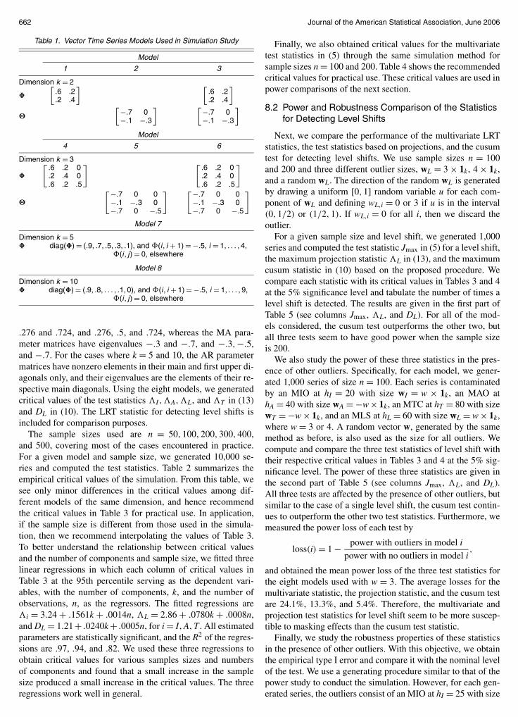
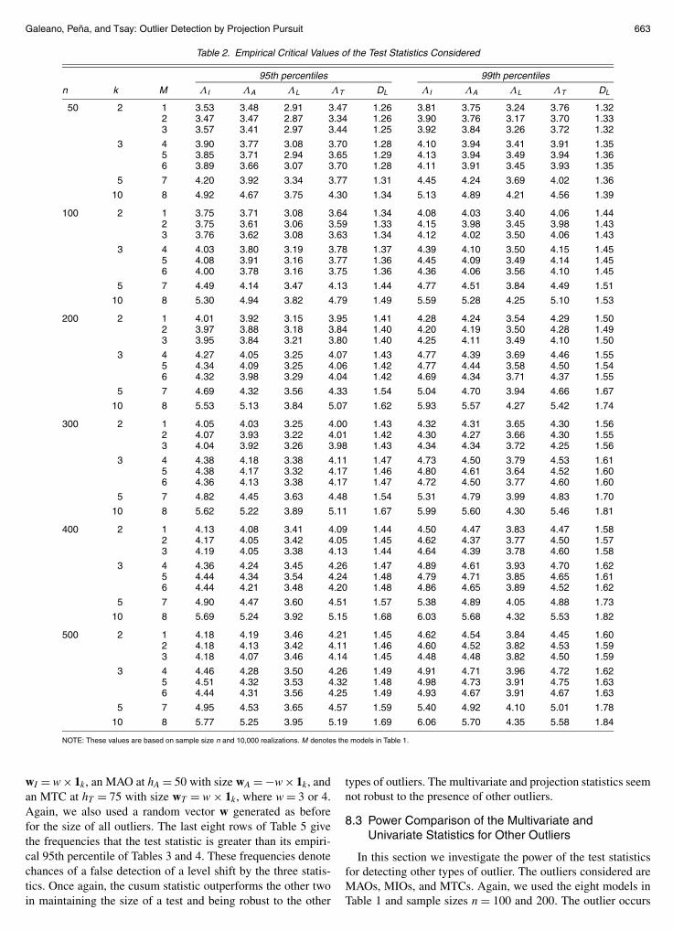
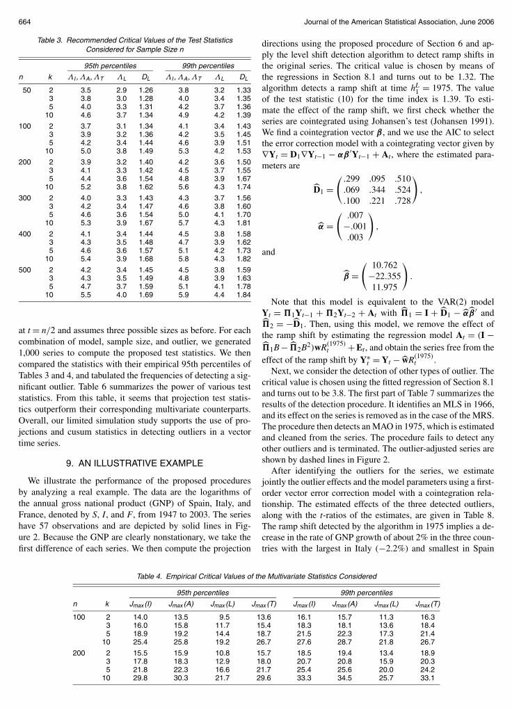
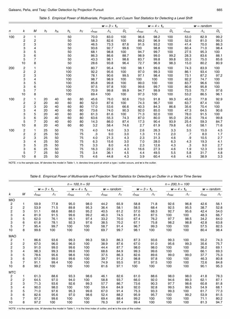
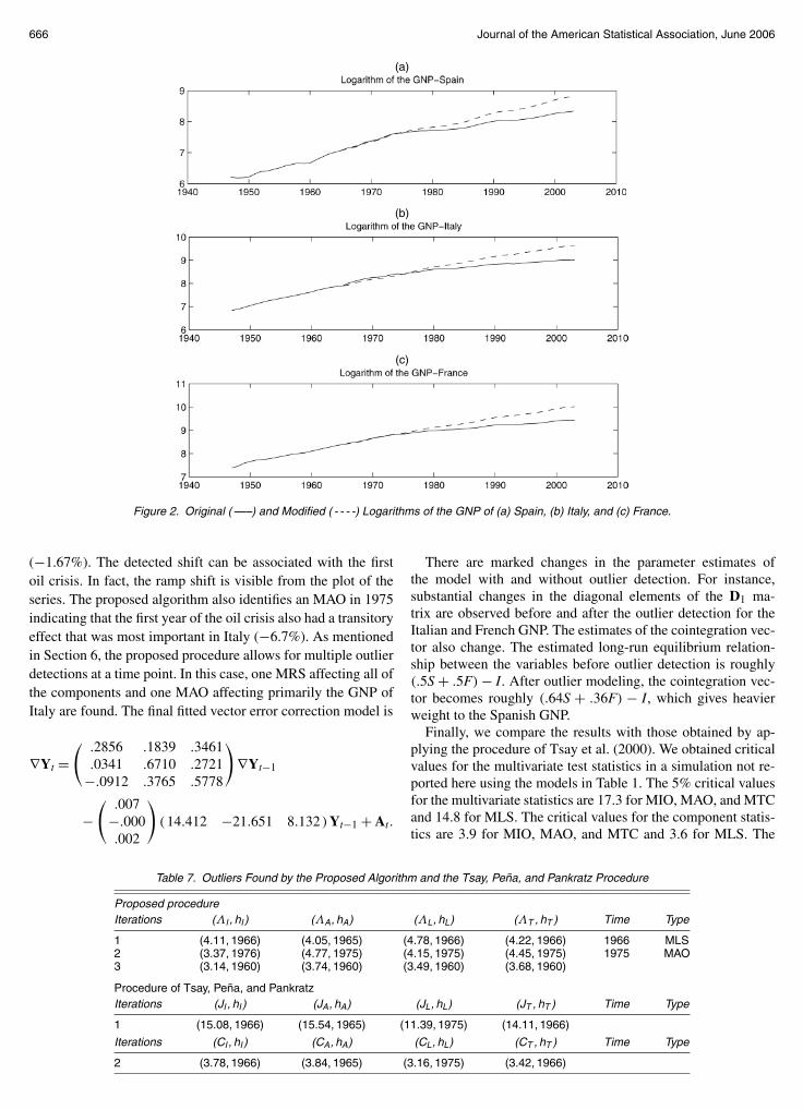
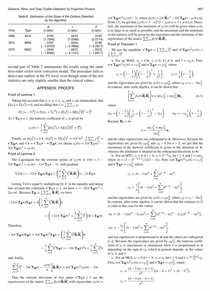