ORIGINAL ARTICLE OpenAccess ... · Keywords: Conditionalcashtransfers;Laborsupply;Juntos;Peru 1...

Fernandez and Saldarriaga IZA Journal of Labor & Development

ORIGINAL ARTICLE Open Access

Do benefit recipients change their laborsupply after receiving the cash transfer?Evidence from the Peruvian Juntos programFernando Fernandez1* and Victor Saldarriaga2

*Correspondence:[email protected] DevelopmentBank, 1300 New York Avenue NW,Washington, D.C. 20577 USAFull list of author information isavailable at the end of the article

Abstract

We investigate the short-term labor supply responses to a Conditional Cash Transfersprogram in Peru. Rather than comparing treated and non-treated households, weexamine how benefit recipients change their labor supply after receiving the cashtransfer. Our empirical strategy exploits exogenous variation in the distance betweenthe program’s payment schedule and interview dates from the Peruvian NationalHousehold Survey. Results suggest that cash recipients reduce their labor supply by6–10 hours in the week following the payment date. This reduction in hours of work islarger for married women and for mothers with children aged 5 or less. In addition,results are robust to different specifications, changes in the sample and a placebo test.

JEL codes: I38, J22Keywords: Conditional cash transfers; Labor supply; Juntos; Peru

1 IntroductionAround the world, Conditional Cash Transfer programs (henceforth, CCTs) are con-sidered powerful means to reduce poverty. By providing monetary transfers to familiesconditional on a set of fulfillments, such as school attendance and health care of chil-dren, the objective of CCTs is twofold. The first is alleviation of current poverty throughperiodical stipends; allowing families to increase overall consumption. The second goalis to reduce future poverty by increasing human capital of children, which is achieved bymeans of program conditionalities.During recent years, CCTs have received a great attention from policymakers and

academics, since significant reductions in poverty levels have been observed after theirimplementation. Furthermore, these programs have been catalogued as one of the mainmodels of safety-nets in developing economies. After the success of programs suchas Bolsa Escola in Brazil and PROGRESA in Mexico “virtually every country in LatinAmerica has such a program” (Fiszbein and Schady 2009).Most of the existing literature on the effects of CCTs has focused on scholastic achieve-

ment, health and nutritional outcomes of children. However, less attention has been paidto the indirect effects that cash transfers could have on adults’ behavior. More specifically,little is known about the effects of CCTs on adult labor supply. While cash transfers arenecessary to accomplish improvements in consumption, education and health, they can

© Fernandez and Saldarriaga; licensee Springer. This is an Open Access article distributed under the terms of the CreativeCommons Attribution License (http://creativecommons.org/licenses/by/2.0), which permits unrestricted use, distribution, andreproduction in any medium, provided the original work is properly cited.

2014, 3:2http://www.izajold.com/content/3/1/2

2014

http://www.izajold.com/content/3/1/2

mailto:[email protected]

http://creativecommons.org/licenses/by/2.0

Fernandez and Saldarriaga IZA Journal of Labor & Development of 30

also generate incentives to reduce work intensity among adults, since this payment can bethought of as a pure income effect.Recent experimental evidence has shown small effects of CCTs on labor supply of

adults from beneficiary households (Parker and Skoufias 2000; Maluccio and Flores 2005;Skoufias and Di Maro 2008; Galasso 2006; Foguel and Paes de Barros 2010). This lit-erature relies on comparisons between beneficiaries and non-beneficiaries to estimatethe so-called average treatment effect of CCTs on labor supply. Nevertheless, there is noevidence on the immediate labor supply response to cash benefits.This article deviates from the previous literature in two subtle but important ways. On

the one hand, this study represents the first attempt to analyze the transitory effects ofwelfare programs, namely CCTs, on labor supply. That is, we do not aim to estimate theaverage treatment effect of CCTs on labor supply. Instead, we are interested in exploringwhether benefit recipients change their labor supply after they receive the cash transfer.On the other hand, we adopt a novel empirical strategy which exploits exogenous varia-tion in the difference between the program’s pay dates and interview dates of a householdsurvey. The combination of pay dates and interview dates allows us to compare beneficia-ries’ labor supply before and after receiving the cash transfer. We think of these deviationsas representing our contribution to the literature on the labor supply responses to cashtransfers.There are several reasons why analyzing immediate labor supply responses to cash

transfers can be of particular interest. First, cash recipients are independent workers andthe available evidence suggests that such workers do not behave according to life-cyclemodels of labor supply but instead they work “one day at a time” (Camerer et al. 1997;Fehr and Goette 2007; Goette et al. 2004). Moreover, these studies argue that indepen-dent workers (who are free to choose when and how much to work) are better describedas having income targets: once they reach their income target they stop working. Second,beneficiaries of CCTs are, by construction, credit constrained. These restrictionsmay pre-vent households to smooth consumption and leisure and, therefore, both variables mayreact to the timing of cash transfers. Indeed, empirical studies have shown that consump-tion of welfare recipients jumps up after the pay date and then declines (Shapiro 2005;Mastrobuoni and Weinberg 2009). Third, benefit recipients of CCTs live in rural areaswhere access to markets is quite limited. In such locations, every time beneficiaries arepaid, they must incur in transportation costs (money but also time). Therefore, theseshort-term responses are relevant for the design of CCTs. In particular, the time that ben-eficiaries spend picking up the money is an opportunity cost that policy makers shouldtake into account when choosing among alternative payment methods (bank depositsversus cash-in-hand) and frequencies (monthly versus bimonthly).We find that cash recipients (female household heads) hours of work are reduced by 6

hours in the week following the pay date. This reduction is rather large, since it impliesa decline of roughly 20% of their weekly hours of work. Moreover, this decrease in hoursof work is larger for married women and mothers with children aged 5 or less. However,no significant effects are found for labor force participation, nor for the probability ofworking for paid activities.We do not find significant effects of cash transfers on the laborsupply of recipients’ partners (when we restrict the sample to married recipients).The document is structured as follows. Related literature is reviewed in Section 2. In

Section 3, we describe the program, named Juntos and its mechanics. Section 4 presents




the econometric set-up and describes the data. Section 5 presents the results and addi-tional robustness checks. In Section 6 we discuss our results and make comparisons withrespect to previous empirical findings. Section 7 concludes.

2 Literature review2.1 Theoretical considerations

Research on labor supply responses to welfare programs has long been a subject of inter-est for economists, especially in developed economies where the expansion of benefittransfer programs to low-income population was initiated during the 1960s. Since then,researchers and policy-makers have been concerned on how welfare programs affectworking incentives of beneficiaries as well as the indirect (unintended) effects thesetransfers may generate on non-targeted population living in localities covered by theprogram.For instance, the effect of welfare programs on labor supply has been widely studied.

The most prominent programs are Aid to Families with Dependent Children (AFDC), theEarned Income Tax Credit (EITC), andmore recently the Food Stamp Program in the U.S.along with the Working Families Tax Credit in the U.K. (see Moffitt 2002 for an extendedreview and discussion). The discussion of how welfare participation affects labor supplyof adults can be divided according to (i) the predicted effects of the canonical model oflabor supply, (ii) program conditions, and (iii) models of household labor supply.The potential effects of benefit transfers can be explained based on the basic static

model of labor supply. In this model, individuals maximize between consumption andleisure facing a budget constraint, which is composed by labor (wage) and non-labor (ini-tial wealth and monetary or in-kind transfers) income. In this study, we focus on theparticular role CCTs can play in determining working incentives1.As pointed out by Alzúa et al. (2013), CCTs have four potential channels through

which adult labor supply could be affected. First, cash transfers represent an incrementin non-labor income. Given that no conditions are imposed with regard to labor effort ofbeneficiaries, this lump-sum transfer is a pure income effect, and therefore, both employ-ment and working hours are expected to decline. Second, program conditions can alsoalter working behavior of adults. For instance, most of the conditions attached to cashtransfer programs imply school enrolment and a maximum number of days accepted forchildren to be absent from school. This increase in school attendance of children allowsparents to augment labor participation and working hours as well, for they avoid allocat-ing time in childcare. Third, if child labor is crucial in determining households’ budgetconstraint, increasing school attendance would also affect adult labor supply. Fourth, cashtransfers can also affect local markets, and thereby, have an indirect impact on non-beneficiaries. Using a sample from the Mexican PROGRESA program, Angelucci and DeGiorgi (2009) find that consumption of ineligible households increases in villages wherethe program was randomly implemented. Alternatively, qualitative studies (Segovia 2001,for example) have described the appearance of fairs ever since CCTs arrived to differentlocalities2.Another important consideration is whether welfare programs impose arbitrary restric-

tions on adult labor supply in order to circumvent working disincentives. Despite theinitial unconditional intent related to working effort, some developed countries haveindexed program benefits according to the labor supply behavior of beneficiaries. For




instance, the Temporary Assistance for Needy Families (TANF) program in the U.S. (for-merly known as the AFDC) initially imposes that at least 20% of TANF recipients in eachState participate in work or work-related activities for a minimum of 20 hours per week.These activities include regular employment, subsidized employment, commuting, on thejob training, and 12 months of vocational training for young beneficiaries aiming to par-ticipate in the labor force. Alternatively, the EITC program, also in the U.S., consists ina refundable tax credit for low- and medium-income families which increases accordingto a standard range of annually labor income and the number of qualifying children inthe family3. These types of cash transfers, both conditional on minimum working hoursor increasing with earned income, act like a contract rigidity, not allowing individuals tomake optimal allocation of working hours. Thus, especially in the case of the EITC wherethe benefit is attached to labor income, the response on individual working effort woulddepend on which of the two possible effects - substitution or income - prevail. Empiricalfindings suggest that it is participation (entry) rather than hours of work which respondsto the EITC4.Unlike these “tied welfare benefits”, CCTs in Latin American do not restrict eligibil-

ity on labor force participation5. This lack of restrictions implies that the looseness ofthe budget constraint due to the welfare benefit introduces a pure income effect, hence,encouraging beneficiaries to demand more leisure. Further, if those individuals barelyineligibles (say because of being just above the poverty line) reduce their working effortin order to narrow down total income and “cheat” the system to become eligibles, thenthe net effect of CCTs on labor supply would depend not only on the amount of reducedworking hours of the ever-eligibles and the formerly ineligibles, but also on the behaviorof the latter group once they have been selected as program beneficiaries and the transferhas been received (e.g., they can return to their initial - optimal - working effort)6.An open question is who in the family actually reduces his working effort. Since cash is

usually transferred to a particular household member (i.e., housewives), it is worth takinginto consideration howwelfare is distributed among familymembers. For this reason, the-oretical considerations of models of household labor supply can also add useful insights.In this line, aside from the potential effects of CCTs on individual adult labor supply, thereexists an open debate on whether families pool their welfare resources. According to thishypothesis, family members act as if they are maximizing a single utility function. Twoseparate models have been developed associated to this “unitary” behavior: the “agree-ment” (Samuelson 1956) and the “dominant family member” frameworks (Becker 1981).Maximizing a single utility function implies that, regardless of who receives the welfare

income, each of the family members would benefit from the monetary transfer throughan intra-family allocation process. In contrast to this “common will” frame, individualcooperative utility models of intra-family bargaining processes (Manser and Brown 1980;McElroy and Horney 1981; and Lundberg and Pollak 1993) as well as non cooperative bar-gaining models (Lundberg and Pollak 1994) have also been postulated. In these models,income is administered by a single agent within the family (for example, the mother) andthus allocation of resources on consumption and leisure could differ across householdmembers.Recent empirical evidence suggests that single cooperative utility functions prevail in

the family bargaining process. Regarding welfare benefits, Lundberg et al. (1997) test thehypothesis of whether families pool their resources exploiting a U.K. policy change which




dictated that child allowances were to be transferred exclusively to wives (mothers). Theauthors find evidence that this policy change induced women to spend more resourceson women’s and children’s clothing relative to men’s clothing. In spite of labor supply,Bertrand et al. (2003) suggest that drops in prime-age men’s labor supply are strongerthan that of prime-age women when the South African pension benefits are received bywomen. In a recent study, Ardington et al. (2009) discuss that pension benefits could, inthe case of perfect resource sharing within the family, reduce hours of work and partici-pation of adults, or in the case of imperfect credit markets, social pensions can be used asa credit support for job seekers.

2.2 Empirical evidence from Latin American countries

To the best of our knowledge, seven empirical studies have been carried out addressingthe potential effects of CCTs on adult labor supply in Latin American countries. Identifi-cation strategies of most of these studies are based on the fact of random treatment (mostof them at the village level) of the CCTs across the targeted population.Parker and Skoufias (2000) exploit the experimental design of the Mexican PROGRESA

program (currently known asOportunidades), which randomly assigned treated and con-trol villages, to address the question of whether CCTs alter labor participation and overallleisure time of adults. The authors find no significant effects of program participation onparticipation rates in the labor force. Instead, they do find that women are more likely toreduce hours allocated to leisure mainly because of program commitments such as takingchildren to schools, health centers and participating in community work.In a later study, Skoufias and Di Maro (2008) evaluate the effects of PROGRESA on

outcomes measuring adult labor supply. Alike Parker and Skoufias (2000) their identifica-tion strategy relies on a difference-in-differences estimation procedure comparing eligibleadults living in treated villages (beneficiaries) versus eligible adults living in non treatedlow-income Mexican villages. The authors do not find statistically significant effects ofprogram participation on the probability of being employed. Moreover, given randomassignment of program deployment across villages, the authors find that cross-sectionalestimates of CCTs on working hours of adults living in treated villages are not statisticallydifferent from working hours of adults living in (randomly) untreated villages.Using a similar estimation methodology for the Nicaraguan Red de Protección Social

(RPS) program,Maluccio and Flores (2005) find that program participation reduces men’s(but not women’s) working effort by 5.5 hours. Maluccio (2010) analyzes the effect of RPSon the overall household labor supply; that is, the sum of each member’s labor intensity.The author finds a negative small but statistically significant effect of the program onhousehold hours of work, especially in agricultural activities, and argues that this reduc-tion can be explained based on the fact that these activities are perhaps associated to lowermarginal rates of return. In contrast, Foguel and Paes de Barros (2010) find no statisti-cally significant effects of six Brazilian programs (Bolsa Escola, Bolsa Alimentação, BolsaFamília, among others) on adult labor supply, neither on the extensive nor the intensivemargins.Galasso (2006) uses propensity score matching and regression discontinuity methods

for evaluating the impact of Chile Solidario on adult labor supply. Although positiveimpacts are found for the take-up of labor market programs, such as re-insertion andtraining programs, the author finds no increments on the share of beneficiaries who are




employed, nor on the share of beneficiaries who have a stable employment. However,increases in participation rates in the labor force are observed only for rural areas.Finally, Alzúa et al. (2013) find negative but small - if not inexistent - effects of three

different programs from Latin American countries (RPS in Nicaragua, PROGRESA inMexico, and Programa de Asignación Familiar in Honduras) on adult labor force par-ticipation and the probability of migrating from agricultural to other working activities.However, they do find a reduction of about 4.7 to 6.3 weekly hours worked in the case ofNicaraguan RPS and a positive and significant effect of Mexican PROGRESA program onmale wages.Most of the aforementioned studies rely on the experimental design of the different

programs evaluated, and most of them (with the exception of Galasso 2006 and Skoufiasand Di Maro 2008) fail to control for the possibility of reallocation of working effortof ineligibles in communities or villages regarding program deployment, as pointed outby Angelucci and De Giorgi (2009). Not taking into account this potential effect mayintroduce negative bias (in absolute terms) to the parameters of interest assuming thatineligibles are more prone to increase their labor intensity given the increase in thedemand for consumable goods and agricultural productive assets in days nearby thetransfer schedules. Because this potential increase in the demand of a particular set ofgoods may increase real wages of ineligibles (introducing a substitution effect), previousempirical findings based on double-difference comparisons are likely to understate thelabor supply responses to CCTs.Unlike previous studies we adopt a different approach to measure labor force variations

as a response to welfare income. In particular, we are interested in exploring whetherworking behavior changes in days near Juntos pay dates. Although this analysis does notallow us to identify average treatment effects of program participation on working effortof adults, it is useful for reconciling theoretical aspects of the canonical labor supplymodel with empirical evidence. The advantage of examining short-term effects of cashtransfers on labor supply of adults is that: (i) it is possible to disentangle income effectsfrom general equilibrium effects often observed in the long run, and (ii) capture effectsof transfers itself and no other effects such as labor supply responses of parents to areduction in child labor introduced by the program.

3 The program and its mechanics3.1 Background

The Peruvian Juntos program was implemented on April 2005 after a period of politicalupheaval and relatively economic stagnation experimented at the beginning of the newcentury during government transition. By 2002, with the new economic reforms broughtup by the former president Alejandro Toledo, the country’s economy began to recoverreaching growth rates above 5% by the mid-2000s. Together, the economic expansion andthe implementation of welfare programs focusing on poverty alleviation and job creationlead to a significant increase of mean per capita income (from US$ 2,450 by 2005 to US$4,050 PPP by the end of year 2010) and, more strikingly, a sharp reduction of roughly 50%of the overall poverty rate which went from 54% in the mid-2000s to 27% by the end ofthe last decade.Particularly, Juntos periodically transfers a stipend to families living in poverty and

extreme poverty conditions, and in return, families must meet certain requirements




including schooling and health care. The program was created with the aim ofstrengthening government presence in remote areas of the country and providing eligiblefamilies with a set of health, nutritional, educational, and identity services, for enhancinghealth and nutritional status of pregnant women and their babies, nursing women, andinfants, as well as fostering human capital accumulation of children under age 14.Juntos is still the most remarkable amid the social welfare programs in Peru, which has

generated the greatest impacts on poverty alleviation and human capital accumulation ofchildren. This can be noticed through the great expansion of the program since it beganto operate. By 2005, almost 22,500 households living in 26 municipalities benefited fromthis program, whereas in 2012 Juntos was deployed in almost 1,011 municipalities, repre-senting roughly 55.2% of the national territory and benefiting 649,553 households livingin poverty and extreme poverty conditions. Recently, Perova and Vakis (2012) found thatJuntos increased overall household income by 43% and was responsible of a 16% and30% decrease in poverty and extreme poverty rates, respectively, in municipalities whereJuntos was initially deployed7.In terms of investments, public expenditures generated by Juntos went from US$ 45

million in 2005 to US$ 177 million in 2007. In this latter year, there was a noticeableexpansion of the program along the Peruvian territory, covering almost 612 more munic-ipalities and more than 400,000 households relative to the 2005 wave. By the end of 2012,public expenditures associated to Juntos were calculated to be almost US$ 225 million.This figure represents roughly 18% of the Peruvian expenditures in safety-net programs.

3.2 Eligibility

Juntos is a means tested program. As Perova and Vakis (2012) clearly describe, selectionof the beneficiary households consists in three steps. The first one is related to selectionof eligible municipalities. This selection is based on five criteria: (i) exposure to violenceduring the late 1980s and early 1990s terrorism era; (ii) poverty level, measured as theproportion of population with unsatisfied needs; (iii) poverty gap; (iv) level of under fivechronic malnutrition; and (v) presence of extreme income poverty.The second step consists in a census of all households in eligible districts collected

by the Instituto Nacional de Estadística e Informática (INEI). A proxy means formulawas used to determine household eligibility, based on poverty. Only households withthe presence of children under age 14 or pregnant women were selected. The algo-rithm for defining eligibility of households is based on a Logit model, which estimatesthe probability of a household living in poverty conditional on a set of observablecharacteristics.Finally, the third stage consists in community validation. This was done in commu-

nity assemblies, carried out by local authorities and representatives of the Ministry ofEducation and Ministry of Health with the aim of minimizing inclusion and exclusionerrors. In general, final selection depends on community validation, and once the house-hold is selected, the housewife (household recipient) must sign a letter in which thehousehold is committed to meet the co-responsibilities, and a health center or post isselected in order for the beneficiaries to make their periodical medical checkups.Once the household is enrolled in the program, transfers are given to the female head

of the household according to the payment schedule defined by the program’s adminis-tration. According to the Peruvian National Household Survey (ENAHO, for its Spanish




acronym), almost 99% of female heads reported to be receiving the transfer on a monthlybasis.

3.3 Components

Initially, the monthly amount was 100 Nuevos Soles (Peruvian local currency). Thisamount is roughly equivalent to US$ 37 (in current dollars). Since 2010, however, theamount was doubled (200 Nuevos Soles) but beneficiaries would receive the cash trans-fer every two months so that the level of the annual amount remained unchanged (1200Nuevos Soles). This change was introduced because of the low rate of money withdrawalfrom bank accounts given the long distances beneficiaries must travel in order to pick upthe money. In our context, the monthly transfer was quite generous, representing over50% of beneficiaries’ monthly per capita household expenditures.Pay dates are defined at the village level which implies that some municipalities have

more than one payment date. Juntos sets a particular day in every village so we have somewithin-municipality variation in payment dates. However, within a district, all paymentsoccur on the same week. This feature of the program does not represent a major problemto our strategy as it will be shown in Section 5.Once they receive the cash, beneficiaries are free to choose how they spend the

money. However, all beneficiaries must meet the following conditions: (i) children of ages6–14 years attend at least 85% school classes; (ii) children of ages 0–59 months get fullyimmunized and visit health centers where their growth is measured and vitamins are pro-vided; (iii) children of ages 3–36 months get nutrition supplements; (iv) pregnant womenvisit health clinics for prenatal care; (v) nursing women visit health centers for postna-tal care; (vi) parents attend health clinics to receive information about nutrition, healthand hygiene; (vii) parents without ID (identification) attend the programMi Nombre (MyName). Juntoswas initially intended as a program of temporary assistance to families, witha duration of 4 years, conditional on households escaping from poverty. Yet, impover-ished households can renew their participation for 4 more years with a benefit reductionof 20%.In 2009 there were two payment methods through which beneficiaries can receive the

cash transfer. The main way to receive the cash was to go to the local branch of thePeruvian National Bank and withdraw themoney (54% of the beneficiaries in our sample).The second way was to go to the main square of the village on the day of payment and waitfor an armored van which contained the money. The difference between these methods isthat the former allows the beneficiary to go to the bank at some other day while the latterdoes not. Moreover, the armored van constitutes a deliver mechanism in which benefi-ciaries do not spend much time in going to withdraw the money. Finally, both systems aremutually exclusive at the village level so beneficiaries do not choose the way they get themoney.

4 Methodology4.1 Econometric model

Differences between Juntos pay dates and ENAHO’s interview dates within a givenmunic-ipality constitute the basis of our empirical strategy. In particular, we will explore whetherlabor supply is reduced in the days near the pay dates. What we do in practice is tocompare beneficiaries, within the same municipality, who are interviewed just after the




payment to those who are not. Given that most households members are engaged in agri-cultural and highly-flexible occupations (i.e., independent workers), it is likely to observethat individuals reduce their working effort in days following the cash receipt.Though we exploit within-municipality variation in interview dates of ENAHO, our

measure of temporal distance is constructed as the difference between pay dates andthe week previous to the survey. This week prior to the interview day is called the“reference week”. When interviewers survey households, they usually ask householdmembers whether they have done specific activities during the last seven days. Forinstance, when asking about labor force participation, interviewers ask the followingquestion: “during the last week, from [day 1] to [interview day], did you have any job?”.Given the way the survey is conducted, all outcomes related to labor supply of surveyedmembers correspond to the seven days prior to the interview day (i.e., the reference week).For the empirical analysis, we construct four dummy variables according to the distance

between the pay day and the reference week. Specifically, the first dummy variable is equalto one if the pay date takes place, at least, two weeks before the reference week, and zerootherwise. Similarly, the second dummy takes the value of one when the pay date occursone week before the reference week, and zero otherwise. The third dummy variable isequal to one if the pay date happens some day during the reference week, and zero oth-erwise. Finally, the fourth dummy variable takes the value of one when the pay date takesplace after the reference week, and zero if not8.We divide the temporal distance between pay dates and interview dates in terms of

weeks for two reasons. First, as pointed earlier, within a given municipality there existsa probability to observe more than one pay date. This is because administrative recordson pay dates are available at the village level, which is the smallest geopolitical unit inPeru. Yet, ENAHO dataset contains geographical identifiers only at the municipality level(which may contain more than one village). This data limitation forces us to collapseadministrative records containing payment dates by village at the municipality level inorder to merge them with the ENAHO dataset. When doing so, almost all villages (99.8%in our sample) within a given municipality are observed to have pay dates during the sameweek. Second, it has been observed that not all beneficiaries withdraw the money on thevery same pay date. For this reason, we assume a rather more parsimonious definitionof temporal distance which allows for some delay in order for beneficiaries to have themoney.When observing a municipality with more than one pay date, we use the earliest pay

date to define the distance between payments and interviews. Though this criterion mayintroduce measurement bias, we also perform additional regressions using the last paydate within the municipalities to re-define temporal distance between payments andinterviews. In Section 5.3, however, we perform an additional sensitivity analysis to checkwhether results hold when using exact payment dates.Figure 1 depicts hours worked in the reference week for distinct groups of beneficia-

ries according to the distance (in weeks) between pay dates and the reference week. Thefirst group is composed of individuals who received the cash transfer two or more weeksbefore they were interviewed (i.e., received the transfer at least two weeks before the ref-erence week). Similarly, the second, third, and fourth groups are composed of individualsfor whom the cash transfer occurred one week before, during, and one week after thereference week, respectively. The decline of hours worked during the reference week is




Figure 1 Hours of work according to the distance between pay and reference week. Notes: Dark greybars correspond to hours of work during the reference week of recipient’s partners. Light grey barscorrespond to hours of work during the reference week of benefit recipients (housewives). Each pair of barsrepresents weekly hours of work according to the temporal distance (in weeks) between the pay andinterview dates. “Two weeks before or more” implies that the payment was observed to occur at least twoweeks before the reference week. “One week before” implies that the payment occurred one week beforethe reference week. “During the reference week” denotes that the payment occurred in some daycorresponding to the reference week. “One week after or more” denotes that the payment will occur oneweek after the individual is surveyed.

linked to the week in which the transfer is received for all individuals included in oursample, and this decline is largest among those who receive the cash transfer one weekbefore the reference week. Furthermore, this decline is larger for cash recipients than fortheir partners. This greater decline in weekly hours worked can be interpreted as contain-ing effects of (i) time spent in going to withdraw the money, (ii) time taken to spent themoney once it is received (i.e., purchasing consumption goods), and (iii) income effects.The first two effects are related to the program’s features, and do not represent disincen-tives to work. Thus, we are particularly interested in isolating the third effect from theoverall labor supply response to welfare transfers.Based on the graphical evidence and exploiting within-municipality differences

between pay dates and interview dates (reference week), we estimate the following model:

yij = α +∑

kδkdij + X′

iβ + λj + μij, (1)

where yij is the outcome variable (labor force participation, hours of work, etc.) of individ-ual i living in municipality j, dij denotes the distance (in weeks) between the payment andthe reference week,Xi is a vector of individual characteristics, λj is a vector ofmunicipalityfixed effects, and μij is an error term capturing all other omitted factors. Our param-eters of interest are denoted by δk , which measures the effect of the distance betweenpay dates and interview dates. Therefore, these parameters are recovered using across-municipalities variation in pay dates and within-municipality variation in interview dates.In what follows, the omitted category is that the payment takes place at least two weeksbefore the reference week (i.e., the first dummy variable).




In this specification, each dummy may capture a specific effect related to the distancebetween pay dates and the reference week. For instance, the second dummy variable,“payment occurs one week before the reference week”, might capture effects related topurchasing consumable goods with the cash received, whereas the third dummy vari-able, “payment occurs during the reference week”, could capture effects related to thetime spent in going to the bank and picking up the money. The fourth dummy variable,“payment occurs one week after the reference week”, may capture additional changes inworking effort of individuals in days prior to the cash transfer.There are some caveats in our empirical strategy which are worth describing with fur-

ther detail. First, we only have information on pay dates established by Juntos but we fail toobserve the actual date the beneficiary went to the bank to withdraw the money. For thisreason, we assume that recipients withdraw the money within the week in which the cashtransfer was made available9. Second, it may be possible that when interviewers arriveto a given municipality, they begin to survey families who work less (i.e., those who arealmost always present at home) and then survey families who work harder. If this were thecase, our estimates should be seen as a lower bound (in absolute terms), since those whowere surveyed earlier are more likely to be captured in the omitted category of distancebetween pay and interview dates, and by construction, all our parameters of interest areinterpreted as a function of the omitted category. Thus, this omitted category capturesthe average working intensity of individuals who were surveyed earlier, and are presumedto have a lower labor intensity10. Finally, our indicators of distance between pay and inter-view dates may capture other effects not related to the transfer but correlated with otherunobservable variables. For instance, it could be the case that pay days are established ondays when labor supply is low for a different reason than the transfer (e.g., holidays). Tocheck this is not the case, we perform falsification tests in Section 5.3.Variation in pay and interview dates is crucial to our strategy. In Table 1, we present the

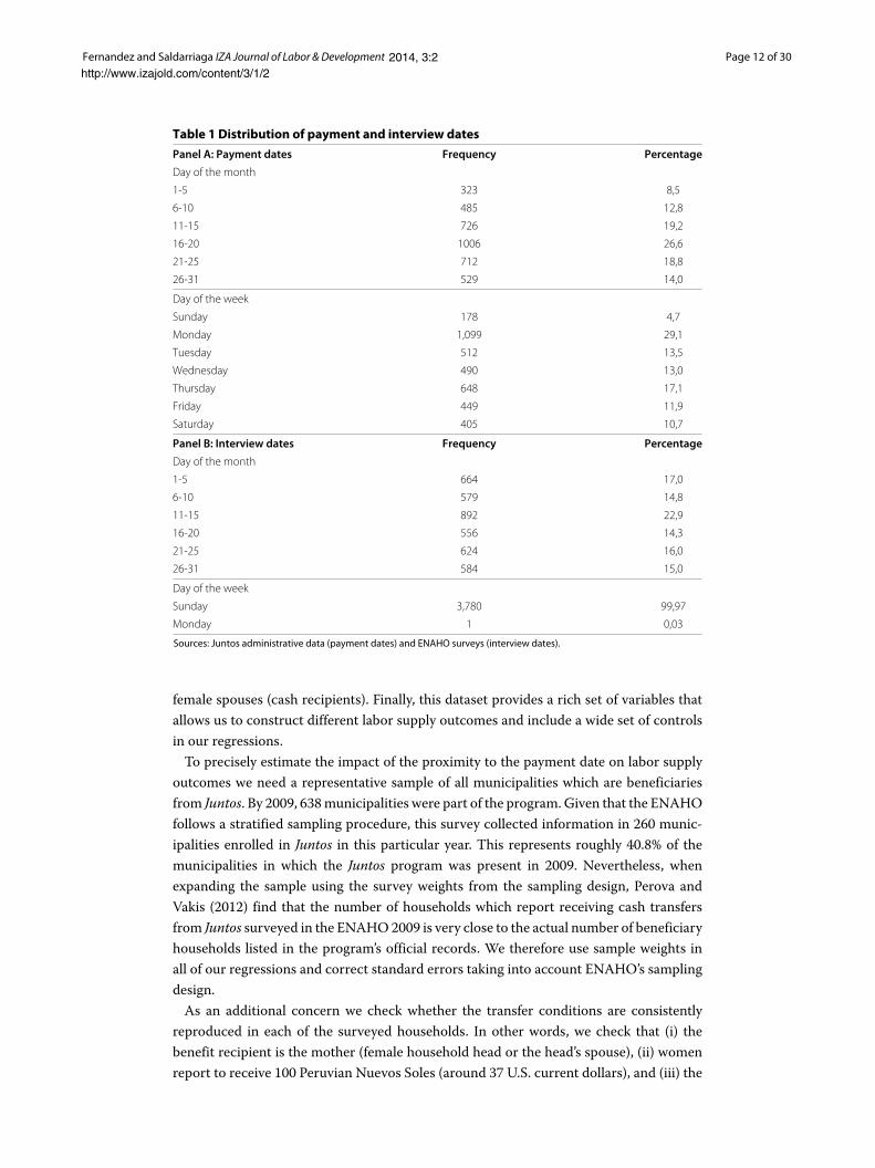
distribution of payment dates associated with the cash transfer from Juntos. Regardingthe day of the month, we do not find any special pattern. If anything, we could say thatthere is a slight concentration around the third week of the month, between the 16th andthe 20th day. Regarding the day of the week, it seems that Mondays are the most commonday of payment while Sundays are the least frequent. The distribution of interview datesis presented in the bottom half of the table. The frequency of dates looks pretty balancedthroughout the month. It is also worth noticing that almost all interviews are conductedon Sundays, when most of the family members stay at home. Finally, the survey processwithin a municipality has an average duration of 30 days.

4.2 Data

Our primary source of information is the ENAHO conducted in 2009 by INEI. TheENAHO collects individual level information and is a nationwide representative survey,both in urban and rural areas. We use information from the employment and incomeregistry, which restricts the sample only for individuals aged 14 or older. The ENAHOhas three important features. First, it includes several questions which allow us to accu-rately identify households receiving monetary transfers from Juntos. This is particularlyimportant since the program design refers to women as the benefit recipients. Second,this survey includes questions regarding relationship with the family head, enabling usto distinguish the potential impact for different household members, say male heads and




Table 1 Distribution of payment and interview dates

Panel A: Payment dates Frequency Percentage

Day of the month

1-5 323 8,5

6-10 485 12,8

11-15 726 19,2

16-20 1006 26,6

21-25 712 18,8

26-31 529 14,0

Day of the week

Sunday 178 4,7

Monday 1,099 29,1

Tuesday 512 13,5

Wednesday 490 13,0

Thursday 648 17,1

Friday 449 11,9

Saturday 405 10,7

Panel B: Interview dates Frequency Percentage

Day of the month

1-5 664 17,0

6-10 579 14,8

11-15 892 22,9

16-20 556 14,3

21-25 624 16,0

26-31 584 15,0

Day of the week

Sunday 3,780 99,97

Monday 1 0,03

Sources: Juntos administrative data (payment dates) and ENAHO surveys (interview dates).

female spouses (cash recipients). Finally, this dataset provides a rich set of variables thatallows us to construct different labor supply outcomes and include a wide set of controlsin our regressions.To precisely estimate the impact of the proximity to the payment date on labor supply

outcomes we need a representative sample of all municipalities which are beneficiariesfrom Juntos. By 2009, 638municipalities were part of the program. Given that the ENAHOfollows a stratified sampling procedure, this survey collected information in 260 munic-ipalities enrolled in Juntos in this particular year. This represents roughly 40.8% of themunicipalities in which the Juntos program was present in 2009. Nevertheless, whenexpanding the sample using the survey weights from the sampling design, Perova andVakis (2012) find that the number of households which report receiving cash transfersfrom Juntos surveyed in the ENAHO2009 is very close to the actual number of beneficiaryhouseholds listed in the program’s official records. We therefore use sample weights inall of our regressions and correct standard errors taking into account ENAHO’s samplingdesign.As an additional concern we check whether the transfer conditions are consistently

reproduced in each of the surveyed households. In other words, we check that (i) thebenefit recipient is the mother (female household head or the head’s spouse), (ii) womenreport to receive 100 Peruvian Nuevos Soles (around 37 U.S. current dollars), and (iii) the




frequency of transfers is monthly. Around 98% of the cash recipients in our sample arewomen satisfying the mentioned conditions.We also check that surveyed households who are receiving monetary transfers from

Juntos satisfy the eligibility conditions. Despite the fact that eligible households should bebelow the poverty line in order to receive the transfer, our sample suggests that around19% of the households are above the poverty line defined by INEI. We exclude non-poorhouseholds from our empirical analysis below and discuss in Section 5.3 how includingthese households can affect our results11.Information on pay dates comes from administrative records provided by Juntos man-

agers12. As mentioned in Section 4.1, payment schedules are reported at the village level.Unique municipality identifiers are used to match the information of payment dates fromthe administrative dataset, previously collapsed at the municipality level, to the benefi-ciaries sample built up from the ENAHO 2009. Our final sample contains information of1,995 individuals living in 1,087 households enrolled in Juntos. Of these individuals, 1,615live in poor conditions, whereas 380 are not poor according to the standard per-capitadaily expenditure measure. Variable averages and standard errors (reported in paren-theses) are shown in Table 2. Each column reports summary statistics of all individualsincluded in each of our four dummy variables defining temporal distance between payand interview dates.

4.3 Outcome variables

We focus on three different measures of labor supply: participation (extensive margin)weekly hours worked (intensive margin) and working for paid activities. As describedabove, each of the outcome variables are measured for the week before (reference week)the interview (which usually takes place on Sundays).Labor participation is a dummy variable which is equal to one when the individual

reported having worked or searching for a job any time during the reference week. Tomeasure labor intensity, we take the total number of hours worked during the same ref-erence week. Lastly, the indicator for working for paid activities is relevant for evidencingchanges in labor supply alternative margins once the payment has already been done or isabout to occur (for instance, household members could reallocate time to family or homeproduction related unpaid activities once the cash has been transferred). The last two out-come variables are defined only for those who reported having been employed during thereference week.Given that we have information of the number of hours worked on each day of the

reference week, we are also able to test whether individuals change their labor supplybehavior in a given day or whether they balance their labor intensity throughout the wholeweek. This insight will be helpful when interpreting our main results.

5 Results5.1 Main results

Table 3 reports the results for the equation of labor force participation. Each row indi-cates the distance between the cash transfer receipt and the reference week. Columns(3), (6), and (9) are our preferred specifications since they control for municipality fixedeffects as well as individual covariates (sex, age, educational level, marital status, indica-tors for mother tongue, indicators for poverty status, an indicator for rural residence, and




Table 2 Descriptive Statistics (according to temporal distance between pay and referenceweek)

Temporal distance between pay and reference week

VariableAt least two weeks One week During the At least one

before before reference week week after

Age 43.53 41.70 42.53 42.27

(12.16) (10.60) (12.29) (11.68)

Male 0.47 0.48 0.46 0.46

(0.50) (0.50) (0.50) (0.50)

Education level: No education 0.19 0.18 0.17 0.19

(0.39) (0.39) (0.38) (0.39)

Education level: Primary 0.60 0.67 0.64 0.63

(0.49) (0.47) (0.48) (0.48)

Education level: Secondary 0.21 0.14 0.18 0.17

(0.40) (0.34) (0.38) (0.37)

Education level: Tertiary 0.01 0.01 0.01 0.01

(0.11) (0.12) (0.11) (0.11)

Mother tongue: Spanish 0.30 0.28 0.33 0.27

(0.46) (0.45) (0.47) (0.44)

Mother tongue: Quechua 0.61 0.71 0.62 0.68

(0.49) (0.46) (0.49) (0.46)

Mother tongue: Other 0.09 0.01 0.05 0.05

(0.28) (0.09) (0.22) (0.22)

Poverty condition: Extremely poor 0.40 0.47 0.43 0.47

(0.49) (0.50) (0.50) (0.50)

Poverty condition: Poor 0.37 0.39 0.36 0.35

(0.48) (0.49) (0.48) (0.48)

Poverty condition: Non poor 0.22 0.14 0.21 0.18

(0.42) (0.35) (0.41) (0.39)

Lives in rural area 0.90 0.77 0.83 0.86

(0.30) (0.42) (0.37) (0.35)

In labor force 0.95 0.93 0.93 0.95

(0.21) (0.25) (0.26) (0.22)

Weekly hours worked 30.66 29.25 30.19 31.77

(15.68) (15.91) (17.97) (16.22)

Worked for paid activities 0.55 0.58 0.53 0.55

(0.50) (0.49) (0.50) (0.50)

Observations 563 425 442 565

interactions between indicators of distance between the payment date and the referenceweek and the dummy variable determining whether or not the individual is the householdhead). Results from these columns suggest that there are no effects of the cash trans-fer receipt on labor force participation, even when splitting the sample by recipients andrecipients’ partners.Table 4 shows results for the equation of hours worked in the reference week. For

the sample as a whole, there are no significant effects on the intensive margin. How-ever, we find that having received the cash transfer within the seven days before thereference week reduces about 5.7 hours of work in the reference week for recipientsonly - see column (6). Recall that the effect of the transfer among recipients maybe driven by two possible confounding factors: time spent in transportation from the




Table 3 Effects of temporal distance between pay and reference week on labor forceparticipation

All individuals Recipients Recipients’ partners

Transferoccurred:

(1) (2) (3) (4) (5) (6) (7) (8) (9)

One weekbefore thereference week

-0.028* -0.009 -0.009 -0.072** -0.044 -0.044 0.015* 0.006 0.148

(0.016) (0.030) (0.030) (0.029) (0.060) (0.060) (0.009) (0.007) (0.203)

During thereference week

-0.027 -0.011 -0.011 -0.054* -0.046 -0.046 0.002 0.019 0.162

(0.017) (0.032) (0.032) (0.029) (0.059) (0.059) (0.012) (0.016) (0.206)

At least one weekafter thereference week

-0.011 -0.007 -0.007 -0.029 -0.024 -0.024 0.010 -0.001 -0.319

(0.014) (0.024) (0.024) (0.024) (0.047) (0.047) (0.010) (0.009) (0.336)

Municipality fixedeffects

No Yes Yes No Yes Yes No Yes Yes

Additionalcontrols

No No Yes No No Yes No No Yes

Observations 1,615 1,615 1,615 859 859 859 756 756 756

R-squared 0.003 0.144 0.144 0.008 0.284 0.284 0.005 0.280 0.280

Notes: Robust standard errors in parentheses. Additional controls include: an indicator for sex, an indicator for marital status(married or living together), age, indicators for educational level (primary, secondary, tertiary), an indicator for Spanishmother tongue, an indicator for poverty status, an indicator for living in rural areas, and interactions terms between anindicator for household head and temporal distance between pay and reference week.***p < 0.01, **p < 0.05, *p < 0.1.

location of residence to the bank and time spent in purchasing the goods or con-suming the money once it has been withdrawn from the bank. If those who werepaid during the reference week have also anticipated the transfer date (and, there-fore, have reduced their working hours) and have spent some time in receiving thetransfer, then the resulting point estimate for those who were paid one week before

Table 4 Effects of temporal distance between pay and reference week on weekly hours ofwork


Transferoccurred:

(1) (2) (3) (4) (5) (6) (7) (8) (9)

One week beforethe referenceweek

-0.558 -1.899 -1.756 -1.640 -4.192* -5. 618** 0.241 -0.425 -0.726

(1.131) (1.840) (1.832) (1.398) (2.284) (2.397) (1.789) (2.903) (2.916)


-0.294 -1.234 -0.972 -0.790 -0.594 -1.836 0.196 -1.537 -1.155

(1.164) (1.849) (1.835) (1.414) (2.213) (2. 367) (1.872) (3.017) (3.012)

At least one weekafter thereference week

1.308 0.678 0.996 0.992 3.802 2.573 1.614 -3.312 -2.332

(1.073) (1.825) (1.806) (1.300) (2.206) (2.295) (1.729) (2.918) (2.919)



Additionalcontrols

No NoZ Yes No No Yes No No Yes

Observations 1,577 1,577 1,577 827 827 827 750 750 750

R-squared 0.002 0.259 0.259 0.005 0.395 0.395 0.001 0.419 0.436

Notes: Robust standard errors in parentheses. See additional notes on Table 3.***p < 0.01, **p < 0.05, *p < 0.1.




the reference week is not driven by these particular confounding effects. Nonetheless,time spent in purchasing goods with the received money could also be affecting ourestimates13.Table 5 reports the results for the equation of “working for paid activities”. Results do

not show a clear pattern regarding the effects of the distance between pay and interviewdates on working in a paid-job, even for different household members. Moreover, theseeffects are statistically insignificant. One possible interpretation for the lack of effects ofthe cash transfer receipt on the probability of working for paid activities is that there mayexist some rigidities in switching from unpaid to paid jobs in the very short run.Given the results, all the remaining analysis is based on the short run effects of cash

transfers on hours of work. In the following lines we try to disentangle the potentialincome effect generated by the welfare transfer from the aforementioned confoundingeffects. To do so, we begin by exploring whether the reduction in working hours broughtup by the welfare transfer is evenly distributed along the whole week or if it is concen-trated in a particular day or days of the reference week. Under the hypothesis that thereduction in hours of work is being driven by time spent in purchasing goods (once wecontrol for the potential anticipation and transportation effects), one should expect thatthe effect of the transfer is grouped in a particular day of the week (say, the day which iscloser to the payment date).In Table 6 we report the resulting coefficients for every day of the reference week. Con-

sistent with the estimates shown in Table 4, we find negative and significant effects forthose who are paid within the seven days before the reference week. Specifically, we findthat working hours are reduced by roughly 1.3 hours in every day except for Sundays. Inaddition, we find that hours of work on Thursday are reduced by 1 hour if payment occursduring the reference week.Overall, results show a decrease in hours worked when payment occurs in the refer-

ence week. This reduction is most likely to be driven by time spent on going to the bank.

Table 5 Effects of temporal distance between pay and reference week on working for paidactivities


Transferoccurred:

(1) (2) (3) (4) (5) (6) (7) (8) (9)

One week beforethe reference week

0.027 0.070 0.070 -0.019 -0.015 -0.015 0.004 0.028 0.027

(0.035) (0.065) (0.065) (0.037) (0.062) (0.062) (0.016) (0.024) (0.024)


-0.020 -0.062 -0.062 -0.030 -0.086 -0.086 -0.026 -0.003 -0.005

(0.037) (0.065) (0.065) (0.037) (0.064) (0.064) (0.021) (0.026) (0.026)

At least one weekafter the referenceweek

0.005 -0.029 -0.029 0.001 -0.081 -0.081 -0.003 0.001 0.010

(0.034) (0.065) (0.065) (0.035) (0.065) (0.065) (0.016) (0.019) (0.021)



Additional controls No No Yes No No Yes No No Yes

Observations 1,577 1,577 1,577 827 827 827 750 750 750

R-squared 0.001 0.047 0.047 0.001 0.358 0.358 0.004 0.402 0.436





Table 6 Effects of temporal distance between pay and reference week on daily hours ofwork (recipients only)

Sunday Monday Tuesday Wednesday Thursday Friday Saturday

Transfer occurred: (1) (2) (3) (4) (5) (6) (7)

One week before the 0.828* -0.732 -0.810* -1.269** -1.319*** -1.334*** -0.982*

reference week (0.452) (0.494) (0.491) (0.498) (0.497) (0.514) (0.535)

During the reference 1.231** -0.183 -0.760 -0.783 -0.994* -0.644 0.297

week (0.500) (0.531) (0.527) (0.520) (0.534) (0.548) (0.552)

At least one week after 1.341*** 0.342 0.225 0.019 -0.084 0.074 0.656

the reference week (0.487) (0.453) (0.458) (0.470) (0.493) (0.459) (0.533)

Municipality fixed effects Yes Yes Yes Yes Yes Yes Yes

Additional controls Yes Yes Yes Yes Yes Yes Yes

Observations 827 827 827 827 827 827 827

R-squared 0.398 0.366 0.395 0.373 0.366 0.379 0.345


However, when payment takes place one week before the reference week, the reductionin labor intensity is evenly distributed along the reference week which is inconsistent withthe hypothesis that our results are mainly driven by transportation from the household tothe bank. We interpret these results as if the dummy variable representing that the pay-ment wasmade “one week before the reference week” reflects the immediate disincentivesto work generated by the having received the cash transfer.

5.2 Heterogeneous effects

We next explore whether the decline in hours worked during the reference week is homo-geneous across all recipients or if they differ according to their observable characteristics.First, in Table 7 we divide the sample of recipients according to their marital status(married and non-married). Interestingly, we find that the reduction in working hours ofrecipients when the transfer was observed to happen one week before the reference weekis driven by the sub-sample of married women. The point estimate for married womenis -11.3 and is statistically significant at the 1% level, whereas the coefficient of the sub-sample of non-married women is not statistically significant. One plausible explanationfor this difference is that married women also rely on their husbands’ income and thisallow them to reduce their working intensity more than non-married women.Second, we analyze if there exists heterogeneity between old and young recipients. In

order to keep a balanced sample in both groups, we say that a recipient is young if sheis 40 years old or younger and she is old, otherwise. Table 8 presents results from thisspecification. Results suggest that younger women (i.e., recipients aged 40 or less) reducemore their working hours relative to older women. In fact, working behavior of olderwomen seems to be unaffected by the cash transfer receipt, since all the coefficients arestatistically insignificant. On the other hand, younger women reduce working intensity byaround 12 hours when the payment occurs one week before the reference week.Third, we distinguish between recipients who have children aged 5 or less and those

who do not. This distinction is important because the presence of young children at homeis a major determinant in female labor supply. Results from splitting the sample accordingto children’s age are presented in Table 9. As expected, recipients with children aged 5 orless reduce their labor supplymore than recipients with older children. The point estimate




Table 7 Effects of temporal distance between pay and reference week on weekly hours ofwork bymarital status (recipients only)

Married Non-married

Transfer occurred: (1) (2) (3) (4)

One week before the reference week -2.318 -11.293*** -2.825 -2.620

(1.875) (3.667) (2.068) (4.647)

During the reference week -2.165 -6.788 0.088 3.899

(2.058) (4.599) (2.325) (4.557)

At least one week after the reference week -1.310 -1.808 3.246 5.252

(1.745) (3.823) (2.023) (4.344)

Municipality fixed effects No Yes No Yes

Additional controls Yes Yes Yes Yes


R-squared 0.072 0.540 0.063 0.540


of having received the cash transfer one week before the reference week is -9.96 hours forrecipients with young children. This could suggest that recipients reduce their hours ofwork in order to spend this additional time in activities related to child rearing.

5.3 Robustness analysis

5.3.1 Changes in the sample and different specifications

Though distance between program’s pay dates and ENAHO’s interview dates is presum-ably exogenous, the estimates in the previous sectionmay be capturing some confoundingeffects. First, the way we construct the temporal distance when observing more than onepay date in a given municipality could introduce measurement bias, attenuating our esti-mated effects. Second, there still some additional effects which have not been discardedin previous estimates, downwardly biasing our results. In particular, the way in whichtime spent in going to withdraw the money can affect the results has not been discussed,and can erroneously be interpreted as a disincentive effect to work. Third, results can besensitive to the inclusion of non-poor beneficiaries in the sample. Finally, our measures

Table 8 Effects of temporal distance between pay and reference week on weekly hours ofwork by age group (recipients only)

Young (under 40) Old


One week before the reference week -4.224** -11.985*** -0.502 -2.088

(2.035) (4.350) (1.919) (4.887)

During the reference week -3.163 -8.396* 0.841 4.143

(2.211) (4.671) (2.186) (4.883)

At least one week after the reference week -0.897 -2.033 1.881 7.796

(1.845) (3.750) (1.893) (4.814)




R-squared 0.061 0.544 0.058 0.553





Table 9 Effects of temporal distance between pay and reference week on weekly hours ofwork by children’s age (recipients only)

With children With children

aged 5 or less aged 6 or more


One week before the reference week -4.346** -9.962** -0.637 -6.152

(1.822) (3.878) (2.209) (4.867)

During the reference week -0.336 -3.830 -2.747 -2.149

(1.903) (4.900) (2.664) (5.689)

At least one week after the reference week 0.686 1.870 -0.624 4.646

(1.618) (3.548) (2.256) (5.791)




R-squared 0.080 0.511 0.042 0.563


of distance between pay and interview dates can be capturing effects other than incomeeffects, affecting the interpretation of our results.We begin our robustness checks by exploring whether the inclusion of non-poor fam-

ilies in our sample could yield different results. To the extent that poor beneficiaries canlive in more remote areas and have less access to transportation, results shown in theprevious section can represent lower-bound estimates. In Table 10 we report the resultsfor weekly hours of work after including non-poor beneficiaries in our sample. Resultscorrespond to recipients only. All the estimated coefficients are negative and statisticallysignificant at the 1% level. In our most preferred specification (i.e., including municipalityfixed effects and controlling for individual characteristics), we find that having been paidone week before the reference week reduces working intensity by around 6 hours.The estimated effects are also larger than those presented in Table 4, where we exclude

non-poor families. This additional evidence suggests that the decline in hours of work isnot driven by the time needed to withdraw the money, since non-poor beneficiaries aremore likely to spend less time going from home to the bank. Moreover, this difference

Table 10 Effects of temporal distance between pay and reference week on weekly hours ofwork, including non-poor beneficiaries (recipients only)

Transfer occurred: (1) (2) (3)

One week before the reference week -2.632 -4.881** -5.998**

(1.329) (2.466) (2.408)

During the reference week -1.564 -0.685 -1.948

(1.319) (2.583) (2.597)

At least one week after the reference week 1.024 3.071 2.251

(1.225) (2.251) (2.275)

Municipality fixed effects No Yes Yes

Additional controls No No Yes

Observations 1,015 1,015 1,015

R-squared 0.009 0.340 0.354





may suggest that non-poor beneficiaries’ labor supply is more elastic (with respect to cashtransfers) than that of poor beneficiaries.As an attempt to dissipate concerns related to measurement errors, we next construct a

different measure of distance between pay and interview dates. Recall that our measure of“recentness” of the cash transfer is defined as the distance in weeks between the pay dateand households’ interview dates within a given municipality. Nevertheless, a municipalitycould have more than one pay date, since Juntos payment schedule is defined at the villagelevel. Up until now, we have used the earliest date to construct our measures of distancebetween pay dates and the reference week.In Table 11 we present results when constructing the indicators of distance using the last

date of payment within the municipality. We only include recipients in the regressions. Incolumns (1) to (3) we exclude non-poor recipients while in columns (4) to (6) we includethem in the sample. When controlling for recipients characteristics, results suggest thatpoor beneficiaries reduce their weekly hours of work by 4.85 (statistically significant atthe 5% level) when the cash transfer occurred one week before the reference week. Thisreduction in weekly hours of work is larger (-5.97 hours) when including non-poor house-holds in the sample (column 6) and is statistically significant at the 5% level. Coefficientsreported in columns (3) and (6) of Table 11 are similar to those reported in column (6) ofTable 4 and column (3) of Table 10, respectively, where we use the same samples and thefirst date of payment within the municipality to define temporal distance. The evidencepresented on this table suggests that the impact of having received the cash transfer oneweek before the reference week on hours of work does not significantly change when wemodify the definition of the municipality-payment date.A major threat to our identification strategy is that the dummy variables denoting the

distance between payment and interview dates may be capturing other factors not relatedto the cash transfer, but to the specific date of the payment. For instance, it could bethe case that payment dates are established on days when the labor supply is low for adifferent reason than the transfer (e.g., holidays). This potential correlation between datesand unobservable variables that affect hours of work would invalidate our strategy. Tocheck that this is not the case, we perform a falsification test using available data fromnon-beneficiaries. If the dummy variables representing the distance between payment

Table 11 Effects of temporal distance between pay and reference week on weekly hours ofwork using the last pay date within municipalities (recipients only)

Poors Poors and non-poors

Transfer occurred: (1) (2) (3) (4) (5) (6)

One week before the reference week -1.229 -3.781 -4.847** -2.118 -5.194* -5.970**

(1.646) (3.171) (2.461) (1.570) (2.983) (2.905)

During the reference week -1.049 1.595 0.817 -1.503 0.803 -0.094

(1.612) (3.344) (3.437) (1.506) (2.957) (3.016)

At least one week after the reference week -0.951 2.238 1.550 -0.450 1.538 1.044

(1.346) (2.718) (2.187) (1.287) (2.536) (2.520)

Municipality fixed effects No Yes Yes No Yes Yes

Additional controls No No Yes No No Yes

Observations 827 827 827 1,015 1,015 1,015

R-squared 0.001 0.392 0.432 0.003 0.339 0.384





and interview dates were correlated with other variables that affect labor supply, theyshould also have an impact on the hours of work of non-beneficiaries.We perform regressions for weekly hours of work including in the sample spouses of

household heads who are not beneficiaries from Juntos but who live in treated munic-ipalities. Table 12 presents the results from these regressions. Results show that noneof the dummies measuring the distance between pay and interview dates are signifi-cant at any conventional level. We interpret these results as if our indicators of distanceare not correlated with omitted variables that may affect labor supply by alternativechannels.Finally, we perform an additional specification that allows us to rule out the hypothesis

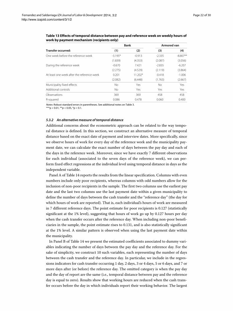
that our results may be driven by the time spent picking up the money. In particular, weperform two separate regressions according to the program’s payment method in orderto rule out this possibility. Recall that there exist two payment methods: deposits to bankaccounts and delivering cash in armored van. The former implies that beneficiaries go tothe bank and withdraw the money through ATM, whereas armored vans distribute themoney to beneficiaries in the main square of their village. This second payment methodwas introduced to reach the most remote places of the Peruvian territory and does notrequire beneficiaries to move long distances in order to pick up the money. Thus, theeffect of temporal distance between interview and payment dates on labor supply for ben-eficiaries who received the cash transfer via armored vans does not contain confoundingfactors such as time spent in withdrawing the money.Table 13 reports the results for weekly hours of work divided according to the pay-

ment mechanism. Columns (1) and (2) correspond to the bank account mechanism, andcolumns (3) and (4) correspond to payment through armored vans. All the regressions areperformed for recipients only. Coefficients for “bank account” are not statistically signifi-cant at any conventional level. In contrast, coefficients for “armored van” are statisticallysignificant at the 1% level when including the full set of controls. In particular, work inten-sity of individuals for whom the cash transfer was made by armored vans is reduced by8.8 hours when the transfer occurred 1 week before the reference week. We interpret thisresult as if the reduction in hours of work is purely due to an income effect and is notrelated to the time spent going to the bank.

Table 12 Effects of temporal distance between pay and reference week on weekly hours ofwork (non-beneficiary housewives)

Transfer occurred: (1) (2) (3)

One week before the reference week -0.054 -0.799 -0.210

(1.542) (3.021) (3.024)

During the reference week -1.603 -2.155 -1.997

(1.557) (2.831) -(2.793)

At least one week after the reference week 3.352 2.211 2.099

(1.663) (2.848) (2.790)

Municipality fixed effects No Yes Yes

Additional controls No No Yes

Observations 927 927 927

R-squared 0.010 0.333 0.348





Table 13 Effects of temporal distance between pay and reference week on weekly hours ofwork by payment mechanism (recipients only)

Bank Armored van


One week before the reference week -3.195* -0.913 -2.335 -8.807**

(1.839) (4.353) (2.087) (3.056)

During the reference week -0.670 7.421 -2.835 -6.207

(2.275) (4.529) (2.119) (3.864)

At least one week after the reference week 0.201 11.202* -0.418 -1.006

(2.082) (6.448) (1.763) (2.667)


Additional controls No Yes Yes Yes


R-squared 0.086 0.478 0.060 0.400


5.3.2 An alternativemeasure of temporal distance

Additional concerns about the econometric approach can be related to the way tempo-ral distance is defined. In this section, we construct an alternative measure of temporaldistance based on the exact date of payment and interview dates. More specifically, sincewe observe hours of work for every day of the reference week and the municipality pay-ment date, we can calculate the exact number of days between the pay day and each ofthe days in the reference week. Moreover, since we have exactly 7 different observationsfor each individual (associated to the seven days of the reference week), we can per-form fixed effect regressions at the individual level using temporal distance in days as theindependent variable.Panel A of Table 14 reports the results from the linear specification. Columns with even

numbers include only poor recipients, whereas columns with odd numbers allow for theinclusion of non-poor recipients in the sample. The first two columns use the earliest paydate and the last two columns use the last payment date within a given municipality todefine the number of days between the cash transfer and the “reference day” (the day forwhich hours of work are reported). That is, each individual’s hours of work are measuredin 7 different reference days. The point estimate for poor recipients is 0.127 (statisticallysignificant at the 1% level), suggesting that hours of work go up by 0.127 hours per daywhen the cash transfer occurs after the reference day. When including non-poor benefi-ciaries in the sample, the point estimate rises to 0.131, and is also statistically significantat the 1% level. A similar pattern is observed when using the last payment date withinthe municipality.In Panel B of Table 14 we present the estimated coefficients associated to dummy vari-

ables indicating the number of days between the pay day and the reference day. For thesake of simplicity, we construct 10 such variables, each representing the number of daysbetween the cash transfer and the reference day. In particular, we include in the regres-sions indicators for cash transfer occurring 1 day, 2 days, 3 or 4 days, 5 or 6 days, and 7 ormore days after (or before) the reference day. The omitted category is when the pay dayand the day of report are the same (i.e., temporal distance between pay and the referenceday is equal to zero). Results show that working hours are reduced when the cash trans-fer occurs before the day in which individuals report their working behavior. The largest




Table 14 Effect of temporal distance between pay and reference day on daily hours ofwork (recipients only)

Payment date within municipalities

Earliest pay date Latest pay date

(1) (2) (3) (4)

Panel A

Coefficient on linear specification 0.127*** 0.131*** 0.119*** 0.123***

(0.014) (0.013) (0.025) (0.039)

[0.523] [0.546] [0.489] [0.557]

Panel B

Transfer occurred (with respect to the reference day):

At least 7 days before 0.157*** 0.109*** 0.123** 0.173***

(0.044) (0.034) (0.041) (0.053)

5or 6 days before -0.288** -0.268* -0.230* -0.196*

(0.116) (0.156) (0.101) (0.091)

3 or 4 days before -0.434** -0.489** -0.339 -0.432**

(0.228) (0.204) (0.243) (0.213)

2 days before -0.251 -0.266 -0.252 -0.209

(0.237) (0.212) (0.212) (0.221)

1 day before 0.053 -0.067 -0.039 0.051

(0.234) (0.209) (0.249) (0.219)

1 day after 0.180 0.174 0.178 0.263

(0.244) (0.219) (0.256) (0.227)

2 days after 0.343 0.313 0.442* 0.448**

(0.247) (0.223) (0.257) (0.230)

3 or 4 days after 0.243 0.203 0.326 0.380*

(0.231) (0.209) (0.242) (0.217)

5 or 6 days after 0.829*** 0.818*** 0.962*** 1.023***

(0.263) (0.241) (0.278) (0.252)

At least 7 days after 1.132*** 1.203*** 1.267*** 1.134***

(0.276) (0.253) (0.294) (0.277)

[0.520] [0.610] [0.519] [0.537]

Individual fixed effects Yes Yes Yes Yes

Observations 5,789 7,105 5,789 7,105

Number of individuals 827 1,015 827 1,015

Notes: Robust standard errors in parentheses. R-squared in brackets.***p < 0.01, **p < 0.05, *p < 0.1.

decline in hours of work occurs when the payment was observed to happen 3 or 4 daysbefore the day of report, and becomes negligible when the pay day gets closer to the dayof report of working behavior.In Figure 2 we plot the estimated coefficients along with their 95% confidence intervals

according to the distance (in days) between the pay day and the reference day. We use day0 (i.e., cash transfer occurred the reference day) as the benchmark dummy variable. Thefigure clearly describes a U-shaped pattern, implying that working intensity is reducedwhen the cash transfer was made within 5 days before the reference day and remains atits normal level when cash transfers occur after the reference day.

6 DiscussionAlong the document, we have argued that, although CCTs may not have long-term orpermanent effects on labor supply of adults, it may be the case that individuals reduce




Figure 2 Coefficients on temporal distance (in days) between pay and reference day. Notes: Each pointin the graph corresponds to a coefficient associated to a dummy variable measuring the temporal distancebetween pay and reference day (day in which the hours of work are reported). The omitted category is“distance between pay and reference day equals 0”, which implies that the pay and the reference day are thesame.

their working intensity in the short-term as a response to welfare transfers. Our empiricalanalysis is based on the plausible assumption that payment schedules of Juntos are orthog-onal to interview dates of ENAHO survey, and, using this identifying assumption, we areable to construct measures of temporal distance to test whether the recentness of cashtransfers affects benefit recipients’ labor supply. In particular, we find that working hoursof recipients are reduced when the cash transfer was observed to happen within one weekbefore the interview took place. In this section we discuss some possible paths throughwhich it is possible to observe short- but not long-term effects of welfare transfers onlabor supply of adults.Results shown in Section 5.3 suggest that declines in working intensity aremostly driven

by married women in their childrearing ages. As discussed by Moffitt (1992), there is avoluminous empirical literature supporting the idea that divorced or separated womenhave a more inelastic labor supply relative to women living in husband-wife (or mari-tally stable) families. There exist several explanations for these observed differences. Theabsence of a male with income to help support the children is the most common expla-nation. Two-parent families not only have the capability of generating more income sinceboth parents can work for paid activities, but can also allocate more efficiently the timedevoted to parenting practices. In contrast, child bearing and work in female-headedhouses are both mutually exclusive activities. Therefore, the income effect generated bythe welfare transfer is more likely to affect women living in husband-wife families.Time not devoted to work can be re-allocated to parenting activities or, more broadly,

home production. However, this implies that activities in which beneficiaries are involvedmight be such that they can freely switch between home production and paid job at anypoint of time (highly flexible activities). In the specific case of the Peruvian Juntos pro-gram, del Pozo and Guzmán (2011) find that the welfare transfers increase the likelihoodof owning small animals, such as poultry and guinea pigs, as well as the use of land for




growing natural grasses (which are used to feed guinea pigs). Moreover, authors findthat income generated by selling small animals as a fraction of household total income isgreater for program beneficiaries relative to non-treated households. Since raising smallanimals has become a profitable business that might be carried out as part of householdactivities, it is likely that program beneficiaries - in particular housewives - have turned tothis activity as a compliment of their home-related duties, and which allow them to earnlabor income while taking care of their children.Aside from the working incentives welfare transfers may generate and the way in which

time is allocated across home production and work effort, it is important to emphasizethat results shown in the empirical analysis correspond to short-term responses of work-ing behavior to welfare transfers and might not be taken as program’s average treatmenteffects. As discussed in the literature review, most of the studies evaluating the effectof CCTs on labor supply (in Latin America) do not find significant changes in workingbehavior of adults. However, “disincentive effects on adult labor supply are found onlyfor the program that made the most generous transfers, the RPS in Nicaragua” (Fiszbeinand Schady 2009). This piece of evidence suggests that income effects generated by wel-fare transfers may depend on the amount of the transfer relative to individual’s earnedincome14.The observed decrease in working effort of recipients in the short run can be explained

from consumption patterns over time. If the welfare transfer allows households to achievea higher consumption bundle over a certain period of time (say, during periods in whichthe cash transfer has recently been made) but not permanently, it is likely that the incomeeffect would be visible only in the short run. However, when the cash transfer has beentotally spent, labor supply must increase in order to afford the initial (i.e., out-of-welfare)consumption bundle. Put it differently, welfare transfers can “buy” leisure as long as a cer-tain level of consumption has been achieved. Below this threshold, labor supply increasesand returns to its initial level. Thus, if the cash transfer is sufficiently large to afford higherlevels of consumption during a long period of time, then this would generate a perma-nent decrease of labor supply of individuals. This insight can explain why CCTs givingmore generous stipends are observed to have disincentive effects on labor supply of adultbeneficiaries.

7 ConclusionIt is well-known that welfare programs in developed countries may have unintendedeffects on labor supply (Ashenfelter 1983; Moffitt 2002). Conditional Cash Transfer pro-grams are not the exception. However, empirical evidence from Latin American countriesdoes not seem to be consistent with the income effect predicted by the standard modelof labor supply. Evidence drawn from experimental and quasi-experimental evaluationmethods is associated with the long term effects of program participation on adult laborsupply. Although these empirical approaches allow researchers to accurately identifyaverage treatment effects of welfare programs on different set of outcomes, it does notcome without its drawbacks. In the specific case of adult labor supply, particular con-cerns should be given to general equilibrium effects potentially introduced by program’sbenefits, and indirect effects generated by the reduction in child labor.In this paper we adopt a novel empirical approach which allow us to estimate short

term effects of cash transfers on adults’ working effort. In particular, we exploit within




municipality exogenous variation introduced by the temporal distance between paymentschedules of the Peruvian Juntos program and interview dates of the Peruvian NationalHousehold Survey to explore whether the monthly receipt of cash transfers affect work-ing behavior. Despite the fact that we cannot estimate average treatment effects, thisempirical approach is useful for isolating immediate effects on labor supply generated byprogram stipends from other potentially confounding factors.We find that women’s (but not men’s) weekly hours of work are reduced by almost 6

hours in the week following the payment date. This effect is mainly driven by married(maritally stable) women and by mothers with children aged 5 or less. However, no effectsare found for labor force participation, nor for working for paid activities. These resultsare robust to changes in the sample, different specifications, and alternative measures oftemporal distance.Some interesting implications arise from our findings. From an academic perspective,

we reconcile empirical evidence with the theoretical predictions of the standard model oflabor supply. In this regard, although income effects are not observed in previous studiesanalyzing the impact of CCTs on adult labor supply in the sense of working disincentives,we do find that, in the short run, these effects are likely to appear. The absence of longterm effects of cash transfers on working effort can be attributed to transfer’s generosityand consumption patterns over time. The latter implies the way households maximizeconsumption in days near pay dates relative to more distant days.For evaluation purposes, special attention should be paid to general equilibrium effects

and changes in the labor market composition potentially introduced by CCTs. Withrespect to the former, it is possible that, within targeted communities, reductions in laborforce participation generated by the introduction of welfare transfers can increase wages,therebymitigating the predicted income effects. In fact, Alzúa et al. (2013) find that house-hold earned income increase as a result of increases in wages among male beneficiarieswhen analyzing the Mexican PROGRESA program. Regarding labor market composi-tion, there is some evidence on changes in working activities. For instance, del Pozo andGuzmán (2011) find that women are more likely to work closer to home. Likewise, Adatoand Roopnaraine (2004) find that adult males work longer in their own parcels relative totheir counterparts when assessing the Nicaraguan RPS.From a policy perspective, different issues arise. First, changing the amount and fre-

quency of the payments could, as suggested by Fiszbein and Schady (2009), amplify theimmediate labor supply response to cash transfers. Second, as an attempt to minimizethe decrease in hours of work, pay dates could be defined on days when labor supplyis expected to be low (e.g., weekends). Third, policy makers should take into accountthe trade-off they face in terms of payment methods: bank deposits can be operationallycheaper but they impose larger transportation costs (not only money but also time) thandelivering cash in armored vans.Finally, we believe that our empirical approach could be useful to answer other

related outcomes that might respond to the receipt of the cash transfer. For instance,we could examine if households change their regular consumption pattern during theweek after the payment (e.g., going to restaurants instead of eating at home). Also, itwould be relevant to check whether cash recipients do not lose control over the moneyonce they arrive home. If potential disputes within the household arise after the pay-ment, we could test whether there is an increase in domestic violence during these




days. It would also be relevant to examine whether children’s school attendance (oreducation-related expenses) increase after the pay date. These are promising avenuesfor future research that may expand the discussion about the benefits and limitationsof CCTs.

Endnotes1In general, welfare programs can be divided according to the type of benefits: cash

and in-kind transfers. Ashenfelter (1983), Moffitt (1992), and Moffitt (2002) provideoutstanding reviews of cash transfer programs. For a review of the relationship betweenin-kind benefits and labor supply, see Currie (1994), Yelowitz (1995), Blundell andMaCurdy (1999), Moffitt (2002), and Hoynes and Schanzenbach (2009).

2Other studies suggest that individuals are likely to invest in agricultural relatedproductive assets. In a recent article, Duflo et al. (2011) document that demand foragricultural tools tend to increase on days close to pay dates

3In order to qualify, children must be 18 years old or under (with few exceptionsaccepting families with children “permanently and totally disabled” aged 19 or above),must be somehow related to the claimant (blood, marriage or law), and must be residentof the United States.

4Other See Eissa and Hoynes (2006) and references therein.5This is not the case for the Chilean Chile Solidario program, since one of the

conditions for eligibility is that unemployed household members should be enrolled inlocal employment offices.

6See Moffitt (2002) for a further examination of this particular scenario.7There does not exist an extensive literature evaluating Juntos impacts on program

beneficiaries. Most of the studies evaluating Juntos are based on qualitative analysis ofprogram’s impacts (Escobal and Benites 2012, Alcázar 2010). Until this date, Perova andVakis (2012), Sánchez and Jaramillo (2012), and del Pozo and Guzmán (2011) constitutethe only quantitative studies of this program. The latter two studies evaluate program’simpacts on nutritional status of infants and household’s productive investments andagricultural production, respectively.

8See the Appendix for further detail on variables definition.9It is worth noting, however, that this would be true only in villages where the

payment method is through bank deposits, but not in villages where beneficiaries go tothe main square on the pay day and wait for the armored van. We use this feature of theprogram to perform additional sensitivity tests in Section 5.3.

10Cash transfers were usually made available during the third week of the month, andinterviews in a given district usually began during the first days of the calendar monthand lasted almost 30 days. Based on this information, those who were interviewed at theend of the month, are more likely to be captured in the dummy variables encompassingindividuals who received the transfer “during the reference week” or “one week after thereference week”.

11The reason underlying the filters of non poor households as part of the Juntosbeneficiaries can be explained based on poverty transitions (households being initiallypoor and then escaping from poverty once they had already been selected asbeneficiaries) and program administrative failures (non poor households selected asbeneficiaries even when the program was initially targeted to households below thepoverty line).

12This information is also available at: http://www.juntos.gob.pe/cronograma_transportadora.php.

13It is worth noting, however, that the reduction in working hours occurs in thereference week. This implies that, if there exists an effect encompassing time spent inconsumption of goods, then it is likely that this effect should appear just after the transferhas been done, but not in the reference week (seven days after the payment date).



http://www.juntos.gob.pe/cronograma_transportadora.php

http://www.juntos.gob.pe/cronograma_transportadora.php


14One important consideration regarding the lack of evidence of negative effects ofwelfare transfers on labor supply is the timing in which program evaluations are made.As discussed by Fiszbein and Schady (2009), most of the existing studies use datacollected shortly after the households have become eligibles to participate in theprogram for the first time. However, it may take some time before households adjusttheir working behavior to welfare benefits.

Appendix

Program’s features

Eligibility Consists of three stages: (i) selection of eligible municipalities (based onpoverty level, under age 5 chronic malnutrition, and exposure to violence during1980s and 1990s); (ii) selection of eligible households (based on Logit modelmeasuring the probability of a household living in poverty); (iii) communityvalidation (community assemblies carried out by local authorities and governmentrepresentatives)

Cash transfer 100 Nuevos Soles (US$ 37) per monthConditions (i) children ages 6–14 attend at least 85% of yearly school classes; (ii) children

ages 0–59 months old get fully immunized and attend periodically to growthcontrols; (iii) children ages 3–36 months get nutrition supplements; (iv) pregnantwomen visit health clinics for prenatal care; (v) nursing women visit health clinicsfor postnatal care; (vi) parents attend health clinics to receive information aboutnutrition, health and hygiene; (vii) parents without ID (identification) attend toprogramMi nombre (My name).

Payment methods (i) bank deposit and (ii) cash delivery with armored van

Variables definition

Reference week Seven days before the interview dayReference day The day of the reference week for which hours of work is reportedFirst pay date The first (earliest) pay date within a municipalityLast pay date The last (latest) pay date within a municipalityOutcomes (i) participation: a dummy variable which is equal to one if the individual had

a job or looked for one in the reference week, and zero otherwise; (ii) hours of work:hours worked in the reference week (or in the reference day); (iii) working for paidactivities: a dummy variable which is equal to one if the individual had a paid-jobin the reference week, and zero otherwise

Variables of temporal distance between pay dates and the reference week (i) paymenttakes place, at least, two weeks before the reference week; (ii) payment occurs oneweek before the reference week; (iii) payment takes place during the reference week;(iv) payment occurs after the reference week. Omitted category: payment takesplace, at least, two weeks before the reference week

Additional samples

Placebo sample Non-treated housewives (female heads who are not enrolled in theprogram) who live in municipalities covered by Juntos




AbbreviationsCCTs: Conditional Cash Transfer programs; Juntos: Conditional Cash Transfer program in Peru; ENAHO: Encuesta Nacionalde Hogares (Peruvian National Household Survey); INEI: Instituto Nacional de Estadistica (Peruvian National Institute ofStatistics).

Competing interestsThe IZA Journal of Labor & Development is committed to the IZA Guiding Principles of Research Integrity. The authorsdeclare that they have observed these principles.

AcknowledgementsThis paper updates and supersedes “Conditional Cash Transfers, Payment Dates and Labor Supply: Evidence from Peru”(available as CEDLAS Working Paper N. 140, Jan. 2013). We are indebted to Leonardo Gasparini for his invaluableguidance, comments and support. We also thank David Lam and an anonymous referee for very useful suggestions onprevious drafts. We are grateful for comments to César Calvo, Viviana Cruzado, Rosamaria Dasso, Albrecht Glitz, MarcGoñi, Hugo Ñopo, Ingo Outes-Leon, Renato Ravina, Laura Ripani, Alan Sánchez, Leopoldo Tornarolli, José Valderrama andseminar participants at the Central Bank of Peru, the LACEA/IDB/WB Network of Inequality and Poverty 2013(UNLP-Argentina), the Peruvian Ministry of Economy and Finance, Universidad de Piura, and Universitat Pompeu Fabra.Nicolás Dominguez provided excellent assistance processing the data on the payment schedule from Juntos. Wegratefully acknowledge financial support from the II Contest of Essays on Labor and Social Issues in Latin America - 2012,organized by CEDLAS (UNLP-Argentina) and IDRC (Canada). All remaining errors are ours.Responsible editor: David Lam

Author details1Inter-American Development Bank, 1300 New York Avenue NW, Washington, D.C. 20577 USA. 2Vancouver School ofEconomics, Vancouver, Canada.

Received: 7 October 2013 Accepted: 5 February 2014Published:

ReferencesAdato M, Roopnaraine T (2004) Sistema de Evaluación de la Red de Protección Social de Nicaragua: Un Análisis Social de

la ‘Red de Protección Social’ (RPS) en Nicaragua. Washington, DC, International Food Policy Research InstituteAlcázar L (2010) Algunas Reflexiones sobre el Programa JUNTOS. In: Portocarrero F, Vásquez E, Yamada G (eds) Politicas

Sociales en el Perú: Nuevos Desafíos. Red para el Desarrollo de las Ciencias Sociales en el PerúAlzúa ML, Cruces G, Ripani L (2013) Welfare programs and labor supply in developing countries: experimental evidence

from Latin America. J Popul Econ 26(4): 1255–1284Angelucci M, De Giorgi G (2009) Indirect effects of an aid program: how do cash transfers affect ineligibles’ consumption?

Am Econ Rev 99(1): 486–508Ardington C, Case A, Hosegood V (2009) Labor supply responses to large social transfers: longitudinal evidence from

South Africa. Am Econ J: Appl Econ 1(1): 22–48Ashenfelter O (1983) Determining participation in income-tested social programs. J Am Stat Assoc 78(383): 517–525Becker GS (1981) Altruism in the family and selfishness in the market place. Economica 48(189): 1–15Bertrand M, Mullainathan S, Miller D (2003) Public policy and extended families: evidence from pensions in South Africa.

World Bank Econ Rev 17(1): 27–50Blundell R, MaCurdy T (1999) Labor supply: a review of alternative approaches. Handb Labor Econ 3: 1559–1695Camerer C, Babcock L, Loewenstein G, Thaler R (1997) Labor supply of New York City Cabdrivers: one day at a time. Q J

Econ 112(2): 407–441Currie J (1994) Welfare and the well-being of children: the relative effectiveness of cash and in-kind transfers. Tax Policy

Econ 8(1): 1–43del Pozo C, Guzmán E (2011) Efectos de las transferencias monetarias condicionadas en la inversión productiva de los

hogares rurales en el Perú. Consorcio de Investigación Económica y Social - CIESDuflo E, Kremer M, Robinson J (2011) Nudging farmers to use fertilizer: theory and experimental evidence from Kenya.

Am Econ Rev 101(6): 2350–2390Eissa N, Hoynes HW (2006) Behavioral responses to taxes: lessons from the EITC and labor supply. Tax Policy Econ 20(1):

73–110Escobal J, Benites S (2012) Transferencias y condiciones: efectos no previstos del programa JUNTOS. Lima: Niños del

Milenio; Young Lives. Boletín de políticas públicas sobre infancia, 7Fehr E, Goette L (2007) Do workers work more if wages are high? Evidence from a randomized field experiment. Am Econ

Rev 97(1): 298–317Fiszbein A, Schady NR (2009) Conditional cash transfers: reducing present and future poverty. World Bank Publications,

Washington DCFoguel M, Paes de Barros R (2010) The effects of conditional transfer programmes on adult labor supply: an empirical

analysis using a time-series-cross-section sample of Brazilian municipalities. Estudios Economicos 40(2): 259–293Galasso E (2006) With their effort and one opportunity: alleviating extreme poverty in Chile. Dev Research Group, World

Bank, Washington DCGoette L, Huffman D, Fehr E (2004) Loss aversion and labour supply. J Eur Econ Assoc 2(2): 216–228. Papers and

Proceedings of the Eighteenth Annual Congress of the European Economic AssociationHoynes HW, Schanzenbach DW (2009) Consumption responses to in-kind transfers: evidence from the introduction of

food stamp program. Am Econ J: Appl Econ 1(4): 109–139Lundberg S, Pollak RA (1993) Separate spheres bargaining and the marriage market. J Pol Econ 101(6): 988–1010Lundberg, S, Pollak RA (1994) Noncooperative bargaining models of marriage. Am Econ Rev 84(2): 132–137


24 Feb 2014



Lundberg S, Pollak RA, Wales TJ (1997) Do husband and wives pool their resources? Evidence from the United Kingdomchild benefit. J Human Resour 32(3): 463–480

Maluccio J (2010) The Impact of Conditional Cash Transfers on Consumption and Investment in Nicaragua. Journal ofDevelopment Studies, Taylor & Francis Journals 46(1): 14–38

Maluccio JA, Flores R (2005) Impact evaluation of a conditional cash transfer program: the Nicaraguan Red de ProtecciónSocial. Research reports 141, International Food Policy Research Institute (IFPRI). Washington DC

Manser M, Brown M (1980) Marriage and household decision-making: a bargaining analysis. Int Econ Rev 21(1): 31–44Mastrobuoni G, Weinberg M (2009) Heterogeneity in intra-monthly consumption patterns, self-control, and savings at

retirement. Am Econ J: Econ Policy 1(2): 163–189McElroy M, Horney MJ (1981) Nash-bargained household decisions: toward a generalization of the theory of demand. Int

Econ Rev 22(2): 333–349Moffitt R (1992) Incentive effects of the US welfare system: a review. J Econ Lit 30(1): 1–61Moffitt, R (2002) Welfare programs and labor supply. Handb Public Econ 4: 2393–2430Parker S, Skoufias E (2000) The impact of Progresa on work, leisure, and time allocation. International Food Policy and

Research Institute, Washington DCPerova E, Vakis R (2012) 5 years in Juntos: new evidence on the program’s short and long-term impacts. Economía 35(69):

53–82Samuelson PA (1956) Social indifference curves. Q J Econ 70(1): 1–22Sánchez A, Jaramillo M (2012) Impacto del programa Juntos sobre la nutrición temprana. Revista Estudios Económicos

23(1): 53–66Segovia G (2001) Efectos del Programa JUNTOS en la Economía Local de las Zonas Rurales a Cinco Años de Intervención

en las Regiones de Apurimac, Ayacucho, Huancavelica y Huánuco. Programa Nacional de Apoyo Directo a los MásPobres - JUNTOS

Shapiro JM (2005) Is there a daily discount rate? Evidence from the food stamp nutrition cycle. J Public Econ 89(1): 303–325Skoufias E, Di Maro V (2008) Conditional Cash Transfers, Adult Work Incentives, and Poverty. Journal of Development

Studies, Taylor & Francis Journals 44(7): 935–960Yelowitz AS (1995) The medicaid notch, labor supply, and welfare participation: evidence from eligibility expansion. Q J

Econ 110(4): 909–939

Cite this article as: Fernandez and Saldarriaga:Do benefit recipients change their labor supply after receiving the cashtransfer? Evidence from the Peruvian Juntos program. IZA Journal of Labor & Development

Submit your manuscript to a journal and benefi t from:

7 Convenient online submission

7 Rigorous peer review

7 Immediate publication on acceptance

7 Open access: articles freely available online

7 High visibility within the fi eld

7 Retaining the copyright to your article

Submit your next manuscript at 7 springeropen.com


10.1186/2193-9020-3-2

2014, 3:2


ORIGINAL ARTICLE OpenAccess ... · Keywords: Conditionalcashtransfers;Laborsupply;Juntos;Peru 1...

Documents

Transcript of ORIGINAL ARTICLE OpenAccess ... · Keywords: Conditionalcashtransfers;Laborsupply;Juntos;Peru 1...