Autoregressive Logistic Regression Applied to Atmospheric...

Climate Dynamics manuscript No.(will be inserted by the editor)

Autoregressive Logistic Regression Applied to Atmospheric CirculationPatterns

Y. Guanche · R. Mınguez · F. J. Mendez

Received: date / Accepted: date

Abstract Autoregressive logistic regression (ALR) mod-1

els have been successfully applied in medical and phar-2

macology research fields, and in simple models to analyze3

weather types. The main purpose of this paper is to intro-4

duce a general framework to study atmospheric circulation5

patterns capable of dealing simultaneously with: seasonal-6

ity, interannual variability, long-term trends, and autocorre-7

lation of different orders. To show its effectiveness on mod-8

eling performance, daily atmospheric circulation patterns9

identified from observed sea level pressure (DSLP) fields10

over the Northeastern Atlantic, have been analyzed using11

this framework. Model predictions are compared with pro-12

babilities from the historical database, showing very good13

fitting diagnostics. In addition, the fitted model is used to14

simulate the evolution over time of atmospheric circula-15

tion patterns using Monte Carlo method. Simulation re-16

sults are statistically consistent with respect to the histor-17

ical sequence in terms of i) probability of occurrence of the18

different weather types, ii) transition probabilities andiii)19

persistence. The proposed model constitutes an easy-to-use20

and powerful tool for a better understanding of the climate21

system.22

Keywords Autoregressive logistic regression· Circulation23

Patterns· Simulation24

R. MınguezEnvironmental Hydraulics Institute, “IH Cantabria”, Universidad deCantabria, C/ Isabel Torres n 15, Parque Cientıfico y Tecnologico deCantabria Santander 39011, SPAINTel.: +34 942 20 16 16Fax: +34 942 26 63 61E-mail: [email protected]

1 Introduction25

The study of atmospheric patterns, weather types or circu-26

lation patterns, is a topic deeply studied by climatologists,27

and it is widely accepted to disaggregate the atmospheric28

conditions over regions in a certain number of represen-29

tative states. This consensus allows simplifying the study30

of climate conditions to improve weather predictions and31

a better knowledge of the influence produced by anthro-32

pogenic activities on the climate system [15–17,29].33

The atmospheric pattern classification can be achieved34

by using either manual or automated methods. Some au-35

thors prefer to distinguish between subjective and objec-36

tive methods. Strictly speaking, both classifications are not37

equivalent because, although automated methods could be38

regarded as objective, they always include subjective deci-39

sions. Among subjective classification methods and based40

on their expertise about the effect of certain circulation pat-41

terns, [13] identify up to 29 different large scale weather42

types for Europe. Based on their study, different classifica-43

tions have been developed, for instance, [10], [11] and [36]44

among others. To avoid the possible bias induced by sub-45

jective classification methods, and supported by the incre-46

ment of computational resources, several automated classi-47

fication (clusterization) methods have been developed, which48

may be divided into 4 main groups according to their math-49

ematical fundamentals: i) threshold based (THR), ii) prin-50

cipal component analysis based (PCA), iii) methods based51

on leader algorithms (LDR), and iv) optimization methods52

(OPT). A detailed description of all these methods and their53

use with European circulation patterns can be found in [29].54

Once the atmospheric conditions have been reduced to55

a catalogue of representative states, the next step is to de-56

velop numerical models for a better understanding of the57

weather dynamics. An appropriate modeling of weather dy-58

namics is very useful for weather predictions, to study the59

2 Y. Guanche et al.

possible influence of well-known synoptic patterns such60

as East Atlantic (EA), North Atlantic Oscillation (NAO),61

Southern Oscillation Index (SOI), etc., as well as to analyze62

climate change studying trends in the probability of occur-63

rence of weather types, and so on. For example, [33] inves-64

tigated long term trends in annual frequencies associated65

with weather types, demonstrating the utility of weather66

classification for climate change detection beyond its short-67

term prognosis capabilities. [26] studied the dynamics of68

weather types using 1st order Markovian and non-Markovian69

models, however seasonality is not considered. [19] intro-70

duced a seasonal Markov chain model to analyze the weather71

in the central Alps considering three weather types. The72

transition probabilities are determined using a linear logit73

regression model. [27] implemented a cyclic Markov chain74

to introduce the influence of the El Nino-Southern Oscilla-75

tion (ENSO).76

Generalized linear regression, and especially autoregressive77

logistic regression, has proved to be a promising framework78

for dealing with seasonal Markovian models, and not only79

for atmospheric conditions. Similar models have been ap-80

plied successfully in medical and pharmacological research81

fields [35,2,30]. The main advantages of autoregressive lo-82

gistic regression (ALR) are that i) it can be used to model83

polytomous outcome variables, such as weather types, and84

ii) standard statistical software can be used for fitting pur-85

poses.86

The aim of this paper is twofold; firstly, to introduce87

autoregressive logistic regression models in order to deal88

with weather types analysis including: seasonality, interan-89

nual variability in the form of covariates, long-term trends,90

and Markov chains; and secondly, to apply this model to91

the Northeastern Atlantic in order to show its potential for92

analyzing atmospheric conditions and dynamics over this93

area. Results obtained show how the model is capable of94

dealing simultaneously with predictors related to different95

time scales, which can be used to predict the behaviour of96

circulation patterns. This may constitute a very powerful97

and easy-to-use tool for climate research.98

The rest of the paper is organized as follows. Section 299

provides the description of Autoregressive Logistic Mod-100

els. In Section 3 the model is applied to the Northeastern101

Atlantic, interpreting results related to the different scales,102

and checking the model’s performance on transition proba-103

bilities and persistence. Finally, Section 4 contains a sum-104

mary and discussion on model performance, possible limi-105

tations and further applications.106

2 Autoregressive Logistic Model107

Traditional uni- or multivariate linear regression models108

assume that responses (dependent variables or outcomes)109

are normally distributed and centered at a linear function110

of the predictors (independent variables or covariates). For111

some regression scenarios, such as the case considered in112

this paper, this model is not adequate because the response113

variableY is categorical and its possible outcomes are as-114

sociated with each weather type (Y ∈ {1,2, . . . ,nwt} being115

nwt the number of weather types), which are not normally116

distributed. Thus the necessity to dispose of alternative re-117

gression models.118

Logistic regression was originally defined as a tech-119

nique to model dependent binary responses ([7,3]). The120

likelihood of the binary dependent outcome is expressed as121

the product of logistic conditional probabilities. [25] intro-122

duced the capability of dealing with transition probabilities123

using Markov chains, which was further explored by [35]124

to predict the outcome of the supervised exercise for in-125

termittent claudication, extending the model to polytomous126

outcomes.127

Let Yt ; t = 1, . . . ,n be the observation weather type at128

timet, with the following possible outcomesYt ∈{1, . . . ,nwt}129

related to each weather type. ConsideringX t ; t = 1, . . . ,n130

to be a time-dependent row vector of covariates with di-131

mensions (1×nc), i.e. seasonal cycle, NAO, SOI, principal132

components of synoptic circulation, long-term trend, etc.,133

the autoregressive logistic model is stated as follows:134

ln

(

Prob(Yt = i|Yt−1, . . . ,Yt−d ,X t)

Prob(Yt = i∗|Yt−1, . . . ,Yt−d ,X t)

)

=

αi +X tβ i +∑dj=1Yt− jγi j; ∀i = 1, . . . ,nwt |i 6= i∗,

(1)

135

whereα i is a constant term andβ i (nc × 1) andγi j ( j =136

1, . . . ,d) correspond, for each possible weather typei, to the137

parameter vectors associated with covariates andd-previous138

weather states, respectively. Note thatd corresponds to the139

order of the Markov model. The model synthesized in equa-140

tion (1) provides the natural logarithm of the probability ra-141

tio between weather typei and the reference weather type142

i∗, conditional on covariatesX t and thed previous weather143

states, i.e. the odds. The left hand side of equation (1) is144

also known aslogit. According to this expression, the con-145

ditional probability for any weather type is given by:146

Prob(Yt = i|Yt−1, . . . ,Yt−d ,X t) =

exp(

αi +Xtβ i +∑dj=1Yt− jγi j

)

nwt

∑k=1

exp

(

αk +Xtβ k +d

∑j=1

Yt− jγk j

) ; ∀i = 1, . . . ,nwt .(2)

147

Note that in order to make parameters unique we im-148

pose an additional condition, which fixes the parameter val-149

ues related to the reference weatheri∗ (arbitrary chosen) to150

zero.151

Autoregressive Logistic Regression Applied to Atmospheric Circulation Patterns 3

2.1 Description of the parameters152

Since the purpose of this paper is to present a unique model153

able to reproduce different weather dynamic characteris-154

tics, including: seasonality, covariates influence, long-term155

trends, and Markov chains; the inclusion of these features156

in the model (1) will be briefly described in this subsection:157

– Seasonality:It is known that there is a strong seasonal-158

ity on weather type frequencies, for example, [19] mod-159

eled this effect for the weather in the central Alps. In160

their work the seasonality is introduced in the model as161

an autoregressive term but it could be also introduced162

by adding harmonic factors. Here, the seasonality is in-163

troduced in the model using harmonics as follows:164

πS = β S0 +β S

1 cos(wt)+β S2 sin(wt) , (3)165

whereπS represents the seasonality effect on thelogit, t166

is given in years,β S0 correspond to annual mean values,167

andβ S1 andβ S

2 are the amplitudes of harmonics,w =168

2π/T is the angular frequency. Sinceβ S0 is a constant169

term, it replaces the independent termα i in (1). For this170

particular case, we chooseT to be defined in years, and171

thus T = 1 andt is in annual scale. This means, for172

instance, that the time associated with day 45 within173

year 2000 is equal to 2000+45/365.25= 2000.1232.174

However, according to the definition of the harmonic175

argument (wt = 2πtT ), t could be given in days, thenT176

must be equal to 365.25.177

Analogously to Autoregressive Moving Average (ARMA)178

models [4], seasonality can also be incorporated trough179

an autoregressive term at lag 365. Details about how to180

incorporate this autoregressive component are given in181

the autoregressive or Markov chain parameters descrip-182

tion below.183

– Covariates: To introduce the effect of different cova-184

riates, the model is stated as follows:185

πC = XβC = (X1, . . . ,Xnc)

βC1...

βCnc

=

nc

∑i=1

XiβCi , (4)

186

whereπC is the covariates effect on thelogit, X is a187

row vector including the values of differentnc cova-188

riates considered (SOI, NAO, monthly mean sea level189

pressure anomalies principal components, etc.), andβC190

is the corresponding parameter vector.191

– Long-term trends: The long-term trend is a very im-192

portant issue because many authors, such as [12,17,5] ,193

perform a linear regression analysis using as predictand194

the probabilities of each weather type, and the time as195

predictor. However, mathematically speaking, this may196

conduct to inconsistencies, such as probabilities outside197

the range 0 and 1, which is not possible. To avoid this198

shortcoming, we use a linear regression model but for199

the logits, being considered as a particular case of co-200

variate:201

πLT = β LT t, (5)202

whereπLT represents the long-term trend effect on the203

logit, andt is given in years. The parameter represents204

the annual rate of change associated with the logarithm205

of the probability for each weather type, divided by the206

probability of the reference weather type, i.e.∆ log pip∗i

.207

The regression coefficientβ LT is a dimensionless pa-208

rameter, which for small values of the coefficient may209

be interpreted as the relative change in the oddsδ pip∗i

due210

to a small change in timeδ t. Note that (5) does not211

correspond to the typical trend analysis because trends212

are analyzed on logits. However, as numerical results213

show, this codification provides consistent results on214

long-term changes of the weather type probabilities.215

– Autoregressive or Markov chain:The sequence of at-216

mospheric circulation patterns can be described as a217

Markov chain. [19] proved that a first order autoregressive218

logistic model is appropriate for reproducing the weather219

types in the central Alps. This effect can be included in220

the model using the following parameterization:221

πARd =d

∑j=1

Yt− jγ j , (6)222

whereπARd represents the autoregressive effect of order223

d on thelogit. The orderd corresponds to the number224

of previous states which are considered to influence the225

actual weather type,Yt− j is the weather type on pre-226

vious j-states, andγ j is the parameter associated with227

previousj-state.228

Note that eachYt− j ; j = 1, . . . ,d in (6) corresponds to229

a different weather type, according to the polytomous230

character of the variable. In order to facilitate parame-231

ter estimation using standard logistic regression tech-232

niques, the autoregressive parts must be transformed233

using a contrast matrix, such as the Helmert matrix [35]234

so that each covariateYt− j transforms intonwt −1 dummy235

variablesZt− j. The Helmer contrast matrix for trans-236

forming outcomeYt into the dummy variable row vector237

Zt is provided in Table 1. According to this transforma-238

tion matrix, equation (6) becomes:239

πARd =d

∑j=1

Yt− jγ j =d

∑j=1

nwt−1

∑k=1

Zt− jk γ jk. (7)

240

Regarding seasonality, and according to expression (7),241

it can be included in the model as follows:242

πAR365 = Yt−365γ365=nwt−1

∑k=1

Zt−365k γ365,k, (8)

243

which corresponds to an autoregressive component at244

lag 365.245

4 Y. Guanche et al.

Yt Zt (1× (nwt −1))

1 −1 −1 −1 . . . −1 −12 −1 −1 −1 . . . −1 13 −1 −1 −1 . . . 2 0...

......

..... .

......

nwt −2 −1 −1 nwt −3 . . . 0 0nwt −1 −1 nwt −2 0 . . . 0 0

nwt nwt −1 0 0 . . . 0 0

Table 1 Helmert Contrast Matrix

Note that the prize for using standard logistic regression246

fitting is an increment on the number of parameters, i.e.247

from d to d× (nwt −1).248

The model can include all these effects adding the log-249

its, i.e.π = πS+πC+πLT +πARd . Thus, expression (2) can250

be expressed as follows:251

Prob(Yt = i|Yt−1, . . . ,Yt−d ,X t) =

exp(

πSi +πC

i +πLTi +πAR

i

)

nwt

∑k=1

exp(

πSk +πC

k +πLTk +πAR

k

)

; ∀i = 1, . . . ,nwt .(9)

252

In order to deal with different time-scales within the253

model: annual, monthly and daily; all the parameters to be254

included are transformed to the lowest scale considered, i.e.255

daily. Thus, we require a covariate value for each day. This256

value may be chosen assuming a piecewise constant func-257

tion over the data period (a month for monthly data, a year258

for yearly data, and so on), which is the one considered259

in this paper, or using interpolation and/or smoothing tech-260

niques, such as splines. Note that in our case, the same co-261

variate value keeps constant for the entire month (during262

30-31 days).263

2.2 Data set-up264

Once the mathematical modeling is defined, this section de-265

scribes the data set-up from the practical perspective. LetY266

correspond to the vector of weather types at different times267

of dimensions (n×1), so thatYt ∈ {1, . . . ,nwt}. To deal with268

polytomous variables a matrixy of dimensions (n× nwt) is269

constructed as:270

yt j =

{

0 if j 6= Yt

1 if j = Yt; ∀ j = 1, . . . ,nwt ; ∀t = 1, . . . ,n. (10)

271

Note that since only one weather type at a time is possi-272

ble,∑nwtj=1 yt j = 1; ∀t. The matrixx of dimensionsn× (3+273

nc + 1+ d × (nwt − 1)) includes all predictors at each of274

the n observations. Three parameters for seasonality (3),275

nc parameters for covariates (4), one parameter for the long276

term trend (5), andd×(nwt −1) parameters for the autocor-277

relation (7). The general data setup for the autoregressive278

logistic regression applied to weather types is provided in279

Table 2.280

Note that the column associated with the seasonality281

constant termβ0 in (3), which corresponds to a column vec-282

tor (1,1, . . . ,1)T , must be included in matrixx depending283

on the standard logistic model used. While some of those284

models automatically include this constant, others do not.285

2.3 Parameter estimation286

Parameter estimation is performed using the maximum like-287

lihood estimator, which requires the definition of the likeli-288

hood function. For a given sequence ofn weather typesY ,289

the likelihood function becomes:290

ℓ(Θ ,Y ,X t) =n

∏t=1

nwt

∏i=1

Prob(Yt = i|Yt−1, . . . ,Yt−d ,X t)uti , (11)

291

whereΘ is the parameter matrix, and the auxiliary variable292

uti is equal to:293

uti =

{

0 if yt 6= i1 if yt = i

; ∀i = 1, . . . ,nwt ; ∀t = 1, . . . ,n. (12)294

Note that the likelihood function (11) is the product of295

univariate logistic functions.296

An important issue for the appropriate modeling of weather297

types, is to decide whether the inclusion of a covariate is298

relevant or not. There are several tests and methods to deal299

with this problem, such as Akaike’s information criteria300

or Wald’s test. Further information related to logistic re-301

gression parameterization and fitting can be found in [8,302

32,34].303

There are several statistical software packages which304

are able to solve a polytomous logistic regression fitting305

(e.g.SYSTAT,NONMEM), but for this particular case, the func-306

tion mnrfit in MATLAB has been used. This function307

estimates the coefficients for the multinomial logistic re-308

gression problem taking as input arguments matricesx and309

y from Table 2.310

3 Case study: Weather types in the Northeastern311

Atlantic312

In the last decade, the availability of long term databases313

(reanalysis, in situ measurements, satellite) allows a de-314

tailed description of the atmospheric and ocean variability315

all over the globe, which include the analysis and study of316

atmospheric patterns. To show the performance of the pro-317

posed model, Daily Sea Level Pressure (DSLP) data from318

NCEP-NCAR database [20] have been used. The area un-319

der study corresponds to the Northeastern Atlantic covering320

latitudes from 25◦ to 65◦N and longitudes from 52.5◦W to321

15◦E. The data record covers 55 years, from 1957 up to322


xAutocorrelation

t Y t y Seasonality Trend Covariates Lag 1 Lag 2 . . . Lagd

t1 Y1 y1,1 . . . y1,nwt cos(wt1) sin(wt1) t1 X1,1 . . . X1,nc Zt−11,1 . . . Zt−1

1,nwt−1 Zt−21,1 . . . Zt−2

1,nwt−1 . . . Zt−d1,1 . . . Zt−d

1,nwt−1


2,nwt−1 Zt−22,1 . . . Zt−2

2,nwt−1 . . . Zt−d2,1 . . . Zt−d

2,nwt−1


3,nwt−1 Zt−23,1 . . . Zt−2

3,nwt−1 . . . Zt−d3,1 . . . Zt−d

3,nwt−1

.

.

....

.

.

....

.

.

....

.

.

....

.

.

....

.

.

....

.

.

....

.

.

....

.

.

....

.

.

....

.

.

.tn Yn yn,1 . . . yn,nwt cos(wtn) sin(wtn) tn Xn,1 . . . Xn,nc Zt−1

n,1 . . . Zt−1n,nwt−1 Zt−2

n,1 . . . Zt−2n,nwt−1 . . . Zt−d

n,1 . . . Zt−dn,nwt−1

Table 2 Data Setup for the Autoregressive Logistic Regression applied to Weather Types

WT1

25

30

35

40

45

50

55

60

65

WT2 WT3

WT4

25

30

35

40

45

50

55

60

65

WT5 WT6

WT7

52.5 45 37.5 30 22.5 15 7.5 0 7.5 1525

30

35

40

45

50

55

60

65

WT8

45 37.5 30 22.5 15 7.5 0 7.5 15

WT9

45 37.5 30 22.5 15 7.5 0 7.5 15

980

1000

1020

1040

Fig. 1 DSLP synoptical patterns associated with the clusterization.

2011. Note that NCEP-NCAR data records start in 1948,323

however it is accepted by the scientific community that324

recorded data up to 1957 is less reliable [21].325

The first step to apply the proposed method is data clus-326

tering. However, in order to avoid spatially correlated vari-327

ables that may disturb the clusterization, a principal com-328

ponents analysis is applied to the daily mean sea level pres-329

sures (DSLP). From this analysis, it turns out that 11 lin-330

early independent components represent 95% of the varia-331

bility.332

As proposed by several authors, such as [6,9] and [22]333

among others, the non-hierarchical K-means algorithm is334

able to classify multivariate patterns into a previously de-335

termined number of groups, eliminating any subjectivity in336

the classification. To reduce the likelihood of reaching lo-337

cal minima with the algorithm, clusterization is repeated a338

hundred times, each with a new set of initial cluster cen-339

troid positions. The algorithm returns the solution with the340

lowest value for the objective function. In this application,341

the daily mean sea level pressures corresponding to the 55342

years of data (n = 20088 days), represented by 11 principal343

components, are classified intonwt = 9 groups.344

Note that in this particular case we select 9 weather345

types for the sake of simplicity, to facilitate the implemen-346

6 Y. Guanche et al.

tation, fit and interpretation of the model results. However,347

the selection of the appropriate number of clusters is an348

open issue not solved yet. There are authors, such as [19,6,349

1], that defend the use of a maximum of 10 weather types,350

others ([23,5,18]) claim that a higher number of weather351

types is required to represent the intrannual/interannualvari-352

ations and seasonality appropriately. Being more specific,353

[6] uses only 4 weather types to represent daily precipita-354

tion scenarios, [9] classifies into 20 weather types the daily355

atmospheric circulation patterns, or for example, [18] uses356

64 weather types to study the extreme wave height variabi-357

lity. This paper does not solve the problem of establishing358

the appropriate number of weather types, which must be359

decided by the user according to his/her experience. But360

due to the facility to implement, fit and interpret model re-361

sults might help establishing a rationale criteria for solving362

this problem.363

Figure 1 shows the 9 representative weather types ob-364

tained from the clusterization. For instance, the upper left365

subplot represents a synoptical circulation pattern with a366

low pressure center above the Britannic Islands while the367

Azores High remains southwestern the Iberian Peninsula,368

whereas the upper central subplot shows the Azores High369

with its center southwest of the United Kingdom.370

Assigning arbitrarily an integer value between 1 and371

nwt = 9, for each weather type in Figure 1, we get the time372

series of weather typesY , which is the input for the model.373

To fit the data and according to the parameterizations374

given in (3)-(7), long-term trend, seasonality, covariates and375

a first order autoregressive Markov chain are included. Each376

study and location may require a pre-process to select the377

parameters to be included according to their influence. Re-378

lated to covariates, it is worth to mention that Monthly Sea379

Level Pressure Anomalies fluctuations (MSLPA) have been380

considered. These anomalies correspond to monthly devia-381

tions from the 55-year monthly averages, which allows ob-382

taining interannual variations. This interannual modulation383

can be related to well known synoptic patterns, such as EA,384

NAO, SOI, etc. [14], but we preferred to use the principal385

components of the anomalies to avoid discrepancies about386

what predictors should be used instead. Nevertheless, we387

could have used those indices within the analysis. In this388

case, the first 9 principal components of the monthly sea389

level pressure anomalies (MSLPA) that explain more than390

96% of the variability are included as covariates. Figure 2391

shows the spatial modes related to those principal compo-392

nents. Note, for instance, that the correlation between the393

first mode and NAO index isr = −0.618 and the correla-394

tion between the second mode and EA synoptic pattern is395

r = 0.482.396

3.1 Model Fitting397

Results obtained from the application of the proposed model398

to the Northeastern Atlantic are described in detail. The399

output given by functionmnrfit is a matrix p of dimen-400

sions (np × (nwt −1)) including parameter estimates by the401

maximum likelihood method, wherenp is the number of402

parameters in the model andnwt is the number of weather403

types considered. Note that each weather type has an as-404

sociated parameter except for the reference weather type,405

whose parameters are set to zero.406

The criteria to choose the final model, i.e. the orderd407

of the auto-regressive component, seasonality, covariates,408

etc. is based on statistical significance, in particular, using409

the likelihood ratio (LR) statistic. This statistical method410

is appropriate to compare nested models by comparing the411

deviance ratio∆Dev., which measures the change of fit-412

ting quality for two different parameterizations, and the413

chi-square distribution with∆d f = ∆np × (nwt − 1) de-414

grees of freedom. Note that∆np is the difference in terms415

of number of parameters for both parameterizations. Ba-416

sically, it tries to check if the increment of fitting quality417

induced by increasing the number of parameters is justi-418

fied, i.e. does the increment on fitted parameters conduct to419

a better model? For instance, assuming a confidence level420

α = 95%, if ∆Dev.> χ20.95,∆d f , the improvement achieved421

by addingnp additional parameters is significant. This test422

allows to analyze which parameters or covariates are rele-423

vant to represent climate dynamics in a particular location.424

In order to evaluate the goodness-of-fit related to the425

predictors, several different fits are considered. In Table3,426

up to 7 nested models are compared depending on the pre-427

dictors involved. In this table, the number of parameters428

(np), the deviance of the fitting (Dev.), the degrees of free-429

dom (df) and the rate of change on deviance (∆Dev.) are430

provided. Model 0 is the so-calledNull model that only431

takes into account an independent term (β0). Model I adds432

the possible influence of seasonality(πS), which according433

to the increment on deviance with respect to the null model434

∆Dev.= 7417> χ295%,16 is significant, confirming the hy-435

phothesis that there is a seasonality pattern in the occur-436

rence of the different weather types. ModelII includes sea-437

sonality and MSLPA covariates (πS +πC), which also pro-438

vide significant information. ModelIII is fitted account-439

ing for seasonality, MSLPA covariates and long-term trend440

(πS + πC + πLT ). In this particular case, the increment on441

quality fit induced by the inclusion of an additional pa-442

rameter, related to long-term trend, is not significant, i.e.443

∆Dev.= 9< χ295%,8. ModelsIV andV include the influ-444

ence of autoregressive terms (Markov Chains, MC) with445

ordersd = 1 and d = 2, respectively (πS + πC + πLT +446

πARd ). Note that both autoregressive components are sig-447

nificant. Additionally, due to the importance of long-term448


EOF 1 (34.5683%)

25

30

35

40

45

50

55

60

65

EOF 2 (28.9207%) EOF3 (16.0923%)

EOF4 (7.2785%)

25

30

35

40

45

50

55

60

65

EOF5 (3.9042%) EOF6 (2.7793%)

EOF7 (1.5346%)

52. 5 45 37. 5 30 22. 5 15 7. 5 0 7.5 1525

30

35

40

45

50

55

60

65

EOF8 (1.0607%)

45 37. 5 30 22. 5 15 7. 5 0 7.5 15

EOF9 (0.67423%)

45 37.5 30 22.5 15 7.5 0 7.5 15 0

-5

0

5

Fig. 2 MSLPA spatial modes related to the Principal Components included as covariates in the model.

changes in the probabilities of occurrence of the different449

weather types, a model that only takes the long term trend450

into account has also been fitted, modelVI (πLT ). This451

additional factor is statistically significant∆Dev.= 69>452

χ295%,8, which means that there is a long-term evolution on453

the probability of occurrence related to each weather type.454

However, there is an inconsistency with respect to model455

III, where this factor is not statistically significant. The rea-456

son for this behaviour is simple, when using covariates, the457

long-term effects are implicitly included in the covariates458

and there is no reason to include additional effects not ex-459

plained by those covariates.460

It is important to point out that deciding which model461

is more appropriate for each case depends on weather dy-462

namics knowledge of the user, and its ability to confront463

or contrast its feeling about which physical phenomena is464

more relevant, with respect to the statistical significanceof465

the corresponding fitted model. The main advantage of the466

proposed method is that it provides an statistical and objec-467

tive tool for deciding what information is more relevant to468

explain climate variability.469

Note that as said in Section 2.1, the seasonality constant470

termβ0, which corresponds to a column vector(1,1, . . . ,1)T471

is automatically included in the model depending on the472

standard logistic model used. Using the functionmnrfit473

this constant is automatically added, thus the null model474

(a) hasnp = 1 and the model fitted only with the trend (g)475

hasnp = 2.476

Model Predictors np df Dev. ∆ Dev. χ295%,∆d f

0 β0 1 160696857367417 26.9

I πS 3 1606807831910214 92.8

II πS +πC 12 160608681059 15.5

III πS +πC +πLT 13 1606006809622159 83.7

IV πS +πC +πLT +πAR1 21 16053645937327 83.7

V πS +πC +πLT +πAR2 29 160472456100 β0 1 16069685736

69 15.5VI πLT 2 16068885667

Table 3 Fitting diagnostics for different model parameterizations, in-cluding number of parameters (np), the deviance of the fitting (Dev.),the degrees of freedom (df) and the rate of change on deviance(∆Dev.)

If we consider modelIV , which accounts for season-477

ality, MSLPA covariates, long-term trend and a first order478

autoregressive component as predictors (πS +πC +πLT +479

πAR1), the model has 21 parameters,np = 21= 3+nc+1+480

d×(nwt −1) = 3+9+1+1×8: i) three for seasonalityπS,481

8 Y. Guanche et al.

ii) nine for the MSLPA principal componentsπC, iii) one482

for the long-term trendπLT , and eight for the dummy vari-483

ables of the first autoregressive componentπAR1.484

Once the parameter estimates for the modelsΘ are known,485

the predicted probabilities ˆp for the multinomial logistic486

regression model associated with given predictors ˜x can487

be easily calculated. This task can be performed using the488

MATLAB function mnrval, which receives as arguments489

the estimated parametersΘ and the covariate values ˜x. In490

addition, confidence bounds for the predicted probabilities491

related to a given confidence level (α = 0.99,0.95,0.90)492

can be computed under the assumption of normally dis-493

tributed uncertainty. Note that these probabilities ˆp cor-494

respond to the probability of occurrence for each weather495

type according to the predictor values ˜x.496

These probabilities allow direct comparison with the497

empirical probabilities from the data, and the possibilityto498

simulate random sequences of weather types. The graphical499

comparison between fitted model and observed data can be500

done in different time scales, aggregating the probabilities501

of occurrence within a year, year-to-year or for different502

values of the covariates (MSLPA).503

– SeasonalityTo analyze the importance of seasonality,504

Figure 3 shows the comparison of the probabilities of505

occurrence for each weather type within a year. Color506

bars represent cumulative empirical probabilities, and507

black lines represent the same values but given by the508

fitted modelI, which only accounts for seasonality us-509

ing harmonics (panel above in Figure 3), and also us-510

ing an autoregressive term at lag 365 (panel below in511

Figure 3). For each day within a year the bars repre-512

sent cumulative probabilities of occurrence of all the 9513

weather types, which are calculated for each day using514

the 55 data associated with each year. Note that there is515

a clear seasonal pattern which is captured by the model516

using harmonics, being circulation patterns 4, 7 and 8517

the most likely weather types during the summer, while518

groups 1, 6 and 9 are more relevant during the winter.519

Comparing both ways of accounting for seasonality, the520

harmonic (panel above of Figure 3) is capable of repro-521

ducing the seasonal behavior better than the autocorre-522

lation term at lag 365 (panel below of Figure 3).523

This seasonal variation through the years is also shown524

in Figure 4. In this particular case color bars represent525

cumulative monthly probabilities. Note that the model526

(black line) repeats the same pattern all over the years527

since we are using fitting results associated with model528

I. Analogously to the previous Figure 3, it is observed529

a clear seasonal pattern. For example, in the lower part530

of the graph it is observed how weather types 1 and531

2, mostly related to winter and summer, respectively,532

change the occurrence probability depending on the sea-533

son within the year. The same behavior is observed in534

0 50 100 150 200 250 300 3500

0.1

0.2

0.3

0.4

0.5

0.6

0.7

0.8

0.9

0

0.1

0.2

0.3

0.4

0.5

0.6

0.7

0.8

0.9

1

Days

Pro

bability

Pro

bability

0 50 100 150 200 250 300 350Days

i) Seasonality with harmonics.

ii) Seasonality with autoregressive term at lag 365

WT1 WT2 WT3 WT4 WT5 WT6 WT7 WT8 WT9 Model 95% CI

Fig. 3 Model fitting diagnostic plot considering seasonality: i) usingharmonics (ModelI), and ii) using an autoregressive term at lag 365.

the upper part of the graph related to weather types 3535

and 9.536

– Mean Sea Level Pressure Anomalies (MSLPA)Al-537

though modelI reproduces and explains the important538

seasonality effect, it can be observed in Figures 3 and 4539

that there are important fluctuations and discrepancies540

between the empirical data and the model on a daily541

and monthly basis, respectively. If modelIV including542

seasonality, MSLPA covariates, an autoregressive com-543

ponent of orderd = 1 and long-term trend (πS +πC +544

πAR1 + πLT ) is considered, results are shown in Fig-545

ures 5 and 6 . The fitted model now explains all fluc-546

tuations both on the daily and monthly scale.547

Note that once the noise on daily and monthly pro-548

babilities is explained by those additional factors, the549

consideration of seasonality through the 365-lag auto-550

regressive model also provides similar diagnostic fitting551

plots, i.e. modelIV : πS +πC +πAR1 +πLR ≡ πAR365+552

πC +πAR1 +πLR.553

554


1980 1985 1990 1995 20000

1

Time

0.8

0.4

0.2

0.6

Pro

bab

ilit

y

WT1 WT2 WT3 WT4 WT5 WT6 WT7 WT8 WT9 Model

Fig. 4 Evolution of the monthly probabilities of occurrence during 20 years and comparison with the seasonal fitted modelI (black line).

0 50 100 150 200 250 300 3500

0.1

0.2

0.3

0.4

0.5

0.6

0.7

0.8

0.9

1

Days

Pro

bability

0

0.1

0.2

0.3

0.4

0.5

0.6

0.7

0.8

0.9

1

Pro

bability

0 50 100 150 200 250 300 350Days

i) Seasonality with harmonics and covariates.

ii) Seasonality with autoregressive term at lag 365 and covariates.


Fig. 5 Model fitting diagnostic plot considering modelIV : i) usingharmonics (ModelI), and ii) using an autoregressive term at lag 365.

It is relevant to point out how the inclusion of MSLPA555

allows explaining the monthly fluctuations on the pro-556

babilities of occurrence associated with the different557

weather types (see Figure 6). These results confirm that558

modelIV is capable of reproducing and explaining the559

weather dynamics accurately, both on a daily and monthly560

basis. Using this model we manage to model atmospheric561

processes on both the short and the long term, using562

a combination of short-term sequencing through auto-563

correlation terms and long-term correlations included564

implicitly through seasonality, covariates and long-term565

variations.566

To further explore the influence of the MSLPA on the567

occurrence probability for each weather type, Figure 7568

shows the probability of occurrence of each weather569

type conditioned to the value of the MSLPA principal570

components (PCi; i = 1, . . . ,9) included as covariates.571

Color bars represent the cumulative empirical proba-572

bilities from data, and the black lines are fitted model573

probabilities.574

According to results shown in Figure 7, the presence or575

absence of a weather type may be related with the value576

of the PC anomaly. For instance, in the subplot associ-577

ated with the first principal component (upper left sub-578

plot), negative values of the principal component im-579

ply an increment on the occurrence of weather types 1580

(red), 6 (maroon) and 9 (grey); while for positive val-581

ues the most likely weather types are 2 (green), 3 (light582

blue) and 5 (yellow). On the other hand, for negative583

values of the second principal component, the domi-584

nant weather type is the blue one (8), prevailing weather585

types 1 and 5 for positive values of the PC. Finally, for586

the third principal component, the behavior is different;587

the lowest values of this principal component indicate a588

higher likelihood of weather types 4 and 9, while higher589

values increase the probability of occurrence of weather590

type 3.591

Note that according to the low variance explained by592

principal component from 4 to 9, we could be tempted593

to omit them from the analysis. To check whether these594

10 Y. Guanche et al.

0

0.5

1

PC1

Pro

bability

PC2 PC3

0

0.5

1

PC4

Pro

bability

PC5 PC6

-5 0 50

0.5

1

PC7

Pro

bability

-5 0 5

PC8-5 0 5

PC9

Fig. 7 Evolution of the probabilities of occurrence of each weathertype conditioned to the principal component value associated withfitted modelIV (black line).

covariates improve significantly the quality of the fit,595

we have included the principal components one at a596

time, and check the likelihood ratio (LR) statistic. Ta-597

ble 4 provides the results from the analysis. Note that598

although it is clear that the most relevant information599

is given by the first three principal components, which600

represent important increments on deviance, the remain-601

der covariates also improve the quality of the model602

from an statistical viewpoint. For this particular case,603

all principal components are statistically significant on604

a 95% confidence level.605

Model df Dev. ∆ Dev. χ295%,8

0 160696857364428 15.5

PC1 160688813083879 15.5

PC2 160680774292292 15.5

PC3 16067275137225 15.5

PC4 16066474912122 15.5

PC5 1606567479061 15.5

PC6 1606487472979 15.5

PC7 1606407465099 15.5

PC8 1606327455118 15.5

PC9 16062474533

Table 4 Fitting diagnostics related to the principal components asso-ciated with MSLPA, including the deviance of the fitting (Dev.), thedegrees of freedom (df) and the rate of change on deviance (∆Dev.)

– Trends Finally, in order to show the possible influence606

of a long-term trends, results associated with modelVI,607

which only accounts for long term trends, are shown608

in Figure 8. Color bars represent the annual probability609

1960 1965 1970 1975 1980 1985 1990 1995 2000 2005 20100

0.1

0.2

0.3

0.4

0.5

0.6

0.7

0.8

0.9

1

Years

Pro

bability

Group 1 Group 2 Group 3 Group 4 Group 5 Group 6 Group 7 Group 8 Group 9 Trends 95% CI

Fig. 8 Annual probabilities of occurrence for each weather type andcomparison with modelV I fitting results (black line) in the period1957−2011.

of occurrence for each year (55 data record) associated610

with the 9 established weather types. The black line611

represents the model fitting (model VI in Table 3). Note612

that we do not present results associated with modelIV613

because the long term trend is not statisticcally signif-614

icant in that model, because long-term effects are im-615

plicitly accounted for through the covariates.616

WT1 WT2 WT3 WT4 WT5 WT6 WT7 WT8

Trend(×10−2) 0.09 -0.4 -0.51 -0.48 -1.330.25 −0.07 −0.16σTrend(×10−2) 0.24 0.21 0.22 0.20 0.24 0.21 0.19 0.19

Table 5 Fitting parameters associated with modelV I including long-term trends, and their corresponding standard error. Values in bold arestatistically significant at 95% confidence level and valuesin cursiveare significant at 90% confidence level.

The parameters for the trends and their corresponding617

standard errors are provided in Table 5. Note that sta-618

tistically significant trends at 95% confidence levels are619

boldfaced, while trends which are statistically signifi-620

cant at 90% confidence level are in italics. According621

to results given in this table the following observations622

are pertinent:623

– The reference weather type is weather type num-624

ber 9. That is the reason why there is no parameter625

related to this case. Note that it is a typical winter626

weather type.627

– The coefficients may be interpreted as the relative628

change in the odds due to a small change in time629

δ t, i.e. the percentage of change in odds between630

weather types 5 and 9 during one year is approxi-631

mately equal to -1.33%.632

– Weather types 4, 7 and 8, which represent summer633

weather types, decrease with respect to type 9. This634

means that weather types related to winter are in-635

creasing its occurrence probability. This result is636


consistent with recent studies about the increment637

of wave climate severity, which is linked to weather638

types during the winter season.639

– Note that weather type 1, also typical during winter,640

slightly increases the odds with respect to type 9.641

Confirming the increment of occurrence related to642

winter weather types.643

3.2 Monte Carlo Simulations644

Once the model has been fitted and the ˆp matrix is ob-645

tained, synthetic sequences of weather types can be gen-646

erated through Monte Carlo method. In this particular case,647

since we require the knowledge of the covariate values dur-648

ing the simulation period, 55 years of daily data series (n=649

20088) are sampled using the original covariates. In order650

to obtain statistically sound conclusions according to the651

stochastic nature of the process, the simulation is repeated652

100 times. The results obtained are validated with a three-653

fold comparison against the original sequence of weather654

types: i) occurrence probabilities of WT, ii) transition prob-655

ability matrix between WT and iii) persistence analysis of656

WT.657

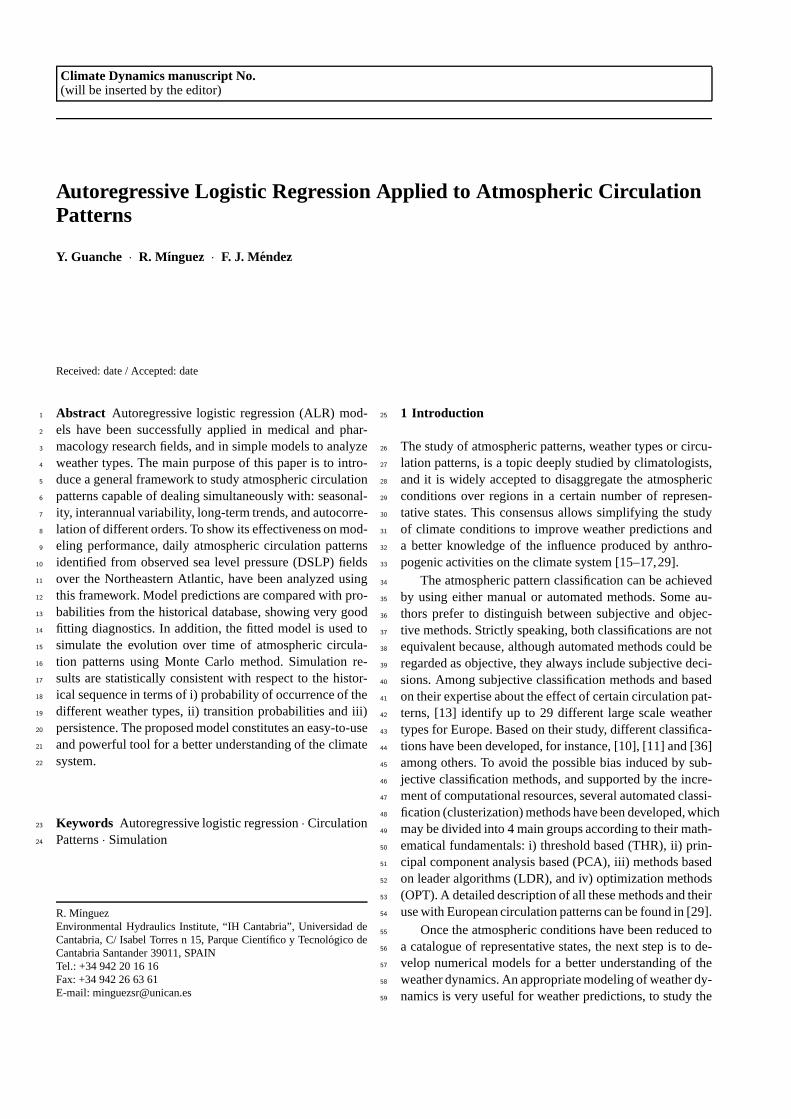
– Occurrence Probabilities658

The probabilities of occurrence of the 9 groups for the659

100 simulations, against the empirical probability of660

occurrence from the 55-year sample data, are shown661

in Figure 9. Note that results are close to the diagonal,662

which demonstrates that the model simulations are ca-663

pable of reproducing the probability of occurrence as-664

sociated with weather types appropriately.665

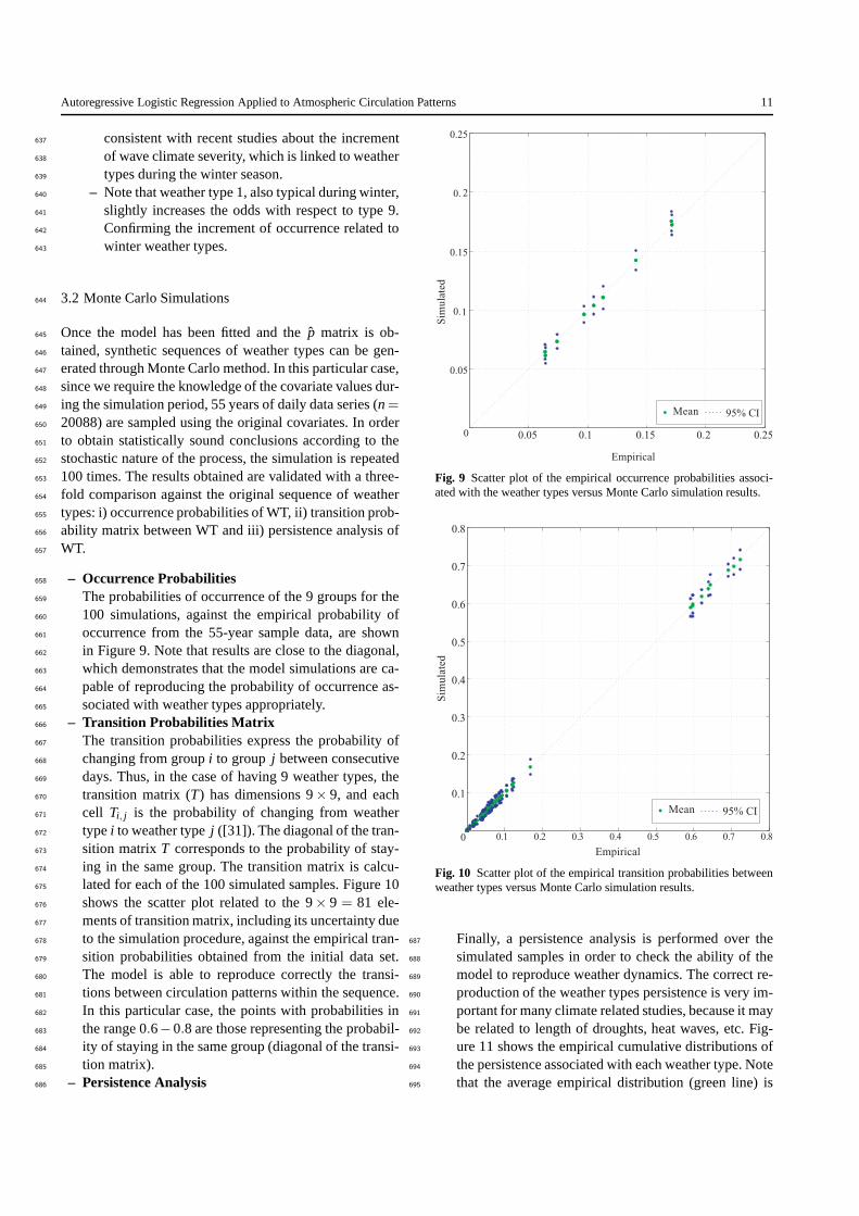
– Transition Probabilities Matrix666

The transition probabilities express the probability of667

changing from groupi to group j between consecutive668

days. Thus, in the case of having 9 weather types, the669

transition matrix (T) has dimensions 9× 9, and each670

cell Ti, j is the probability of changing from weather671

typei to weather typej ([31]). The diagonal of the tran-672

sition matrixT corresponds to the probability of stay-673

ing in the same group. The transition matrix is calcu-674

lated for each of the 100 simulated samples. Figure 10675

shows the scatter plot related to the 9× 9 = 81 ele-676

ments of transition matrix, including its uncertainty due677

to the simulation procedure, against the empirical tran-678

sition probabilities obtained from the initial data set.679

The model is able to reproduce correctly the transi-680

tions between circulation patterns within the sequence.681

In this particular case, the points with probabilities in682

the range 0.6−0.8 are those representing the probabil-683

ity of staying in the same group (diagonal of the transi-684

tion matrix).685

– Persistence Analysis686

0.05 0.1 0.15 0.2 0.250

0.05

0.1

0.15

0. 2

0.25

Empirical

Sim

ula

ted

Mean 95% CI

Fig. 9 Scatter plot of the empirical occurrence probabilities associ-ated with the weather types versus Monte Carlo simulation results.

0.1 0.2 0.3 0.4 0.5 0.6 0.7 0.8

0.1

0.2

0.3

0.4

0.5

0.6

0.7

0.8

0

Empirical

Sim

ula

ted

Mean 95% CI

Fig. 10 Scatter plot of the empirical transition probabilities betweenweather types versus Monte Carlo simulation results.

Finally, a persistence analysis is performed over the687

simulated samples in order to check the ability of the688

model to reproduce weather dynamics. The correct re-689

production of the weather types persistence is very im-690

portant for many climate related studies, because it may691

be related to length of droughts, heat waves, etc. Fig-692

ure 11 shows the empirical cumulative distributions of693

the persistence associated with each weather type. Note694

that the average empirical distribution (green line) is695


0

0.5

1WT1 WT2 WT3

WT4 WT5 WT6

WT7 WT8 WT9

Pro

bab

ilit

y

0

0.5

1

Pro

bab

ilit

y

0

0.5

1

Pro

bab

ilit

y

0 10 20Days Days Days

0 10 20

Empirical data Simulations95% CI

0 10 20

Fig. 11 Empirical cumulative distribution of the persistence for the 9groups related to: i) historical data and ii) sampled data using MonteCarlo method.

very close to the one related to the historical sample696

data (blue line) for all cases. This blue line stays be-697

tween the 95% confidence intervals (red dotted line)698

related to the 100 simulations. To further analyze the699

performance on persistence from an statistical view-700

point, we perform a two-sample Kolmogorov-Smirnov701

([24]) goodness-of-fit hypothesis test between the orig-702

inal data and each sampled data. This test allows de-703

termining if two different samples come from the same704

distribution without specifying what that common dis-705

tribution is. In Figure 12 the box plots associated with706

the p-values from the 100 tests for each weather type707

are shown. Note that if thep-value is higher than the708

significance level (5%) the null hypothesis that both709

samples come from the same distribution is accepted.710

Results shown in Figure 12 prove that for most of the711

cases the persistence distributions from the Monte Carlo712

simulation procedure come from the same distribution713

as the persistence distribution from the historical data.714

For all the weather types the interquartile range (blue715

box) is above the 5% significance level (red dotted line).716

These results confirm the capability of the model to re-717

produce synthetic sequences of weather types coherent718

in term of persistence.719

4 Conclusions720

This work presents an autoregressive logistic model which721

is able to reproduce weather dynamics in terms of weather722

types. The method provides new insights on the relation723

between the classification of circulation patterns and the724

0

0.1

0.2

0.3

0.4

0.5

0.6

0.7

0.8

0.9

1

p-v

alu

e

Weather type

1 2 3 4 5 6 7 8 95% significance level

Fig. 12 Box plot associated with thep-values from the 100 tests foreach weather type.

predictors implied. The advances with respect to the state-725

of-the-art can be summarized as follows:726

– The availability of the model to include autoregressive727

components allows the consideration of previous time728

steps and its influence in the present.729

– The models allows including long-term trends which730

are mathematically consistent, so that the probabilities731

associated with each weather type always range between732

0 and 1.733

– The proposed model allows to take into account simul-734

taneously covariates of different nature, such as MSLPA735

or autoregressive influence, where the time scales are736

completely different.737

– The capability of the model to deal with nominal clas-738

sifications enhances the physical point of view of the739

problem.740

– The flexibility of the proposed model allows the study741

of the influence of any change in the covariates due to742

long-term climate variability.743

On the other hand, the proposed methodology presents744

a weakness in relation with the data required for fitting pur-745

poses, because a long-term data base is needed to correctly746

study the dynamics of the weather types.747

Although further research must be done on the applica-748

tion of the proposed model to study processes that are di-749

rectly related with weather types, such as marine dynamics750

(wave height, storm surge, etc.) or rainfall, this method pro-751

vides the appropriate framework to analyze the variability752

of circulation patterns for different climate change scenar-753

ios ([28]).754

Acknowledgements This work was partially funded by projects “AM-755

VAR” (CTM2010-15009), “GRACCIE” (CSD2007-00067, CONSOLIDER-756

INGENIO 2010), “IMAR21” (BIA2011-2890) and “PLVMA” (TRA2011-757

28900) from the Spanish Ministry MICINN, “MARUCA” (E17/08)758

from the Spanish Ministry MF and “C3E” (200800050084091) from759

the Spanish Ministry MAMRM. The support of the EU FP7 Theseus760


“Innovative technologies for safer European coasts in a changing cli-761

mate”, contract ENV.2009-1, n. 244104, is also gratefully acknowl-762

edged. Y. Guanche is indebted to the Spanish Ministry of Science763

and Innovation for the funding provided in the FPI Program (BES-764

2009-027228). R. Mınguez is also indebted to the Spanish Ministry765

MICINN for the funding provided within the “Ramon y Cajal” pro-766

gram.767

References768

1. van den Besselaar, E., Klein Tank, A., van der Schrier, G.:In-769

fluence of circulation types on temperature extremes in Europe.770

Theoretical and Applied Climatology99, 431–439 (2009)771

2. Bizzotto, R., Zamuner, S., De Nicolao, G., Karlsson, M.O.,772

Gomeni, R.: Multinomial logistic estimation of Markov-chain773

models for modelling sleep architecture in primary insomnia pa-774

tients. Pharmacokinet Pharmacodyn37, 137–155 (2010)775

3. Bonney, G.E.: Logistic regression for dependent binary data.776

Biometrics43(4), 951–973 (1987)777

4. Box, G.E.P., Jenkins, G.M., Reinsel, G.C.: Time Series Analysis:778

Forecasting and Control. Prentice-Hall International, New Jersey,779

NJ (1994)780

5. Cahynova, M., Huth, R.: Enhanced lifetime of atmosphericcir-781

culation types over europe: fact or fiction? Tellus61A, 407–416782

(2009)783

6. Corte-Real, J., Xu, H., Qian, B.: A weather generator for obtain-784

ing daily precipitation scenarios based on circulation patterns.785

Climate Research13, 61–75 (1999)786

7. Cox, D.R.: The analysis of multivariate binary data. Journal of787

the Royal Statistical Society. Series C (Applied Statistics)21(2),788

113–120 (1972)789

8. Dobson, A.J.: An Introduction to Generalized Linear Models,790

second edn. Chapman & Hall/CRC, Florida (2002)791

9. Esteban, P., Martın-Vide, J., Mases, M.: Daily atmospheric cir-792

culation catalogue for Western Europe using multivariate tech-793

niques. International Journal of Climatology26, 1501–1515794

(2006)795

10. Gerstengarbe, F.W., Werner, P.: Katalog der Grosswetterlagen796

Europas(1881-1998) nach Paul Hess und Helmuth Brezowsky.797

Potsdam Institut fur Klimafolgenforschung, Postdam, Germany798

(1999)799

11. Gerstengarbe, F.W., Werner, P.: Katalog der Grosswetterlagen800



(2005)803

12. Goodess, C.M., Jones, P.D.: Links between circulation and804

changes in the characteristics of Iberian rainfall. International805

Journal of Climatology22, 1593–1615 (2002)806

13. Hess, P., Brezowsky, H.: Katalog der Grosswetterlagen Eu-807

ropas(Catalog of the European Large Scale Weather Types). Ber.808

Dt. Wetterd, in der US-Zone 33, Bad Kissingen, Germany (1952)809

14. Hurrell, J., Kushnir, Y., Ottersen, G., Visbeck, M.: TheNorth810

Atlantic Oscillation: Climate Significance and Environmental811

Impact, geophysical monograph series 134. American Geophys-812

ical Union, Washington, DC (2003)813

15. Huth, R.: A circulation classification scheme applicable in GCM814

studies. Theoretical and Applied Climatology67, 1–18 (2000)815

16. Huth, R.: Disaggregating climatic trends by classification of cir-816

culation patterns. International Journal of Climatology21, 135–817

153 (2001)818

17. Huth, R., Beck, C., Philipp, A., Demuzere, M., Ustrnul, Z.,819

Cahynova, M., Kysely, K., Tveito, O.E.: Classification ofatmo-820

spheric circulation patterns. Trends and Directions in Climate821

Research1146, 105–152 (2008)822

18. Izaguirre, C., Menendez, M., Camus, P., Mendez, F.J.,823

Mınguez, R., Losada, I.J.: Exploring the interannual va-824

riability of extreme wave climate in the northeast atlantic825

ocean. Ocean Modelling59–60, 31–40 (2012). DOI826

http://dx.doi.org/10.1016/j.ocemod.2012.09.007827

19. Jordan, P., Talkner, P.: A seasonal Markov chain model for the828

weather in the central Alps. Tellus52A, 455–469 (2000)829

20. Kalnay, E.M., Kanamitsu, R., Kistler, W., Collins, D., Deaven,830

L., Gandin, M., Iredell, S., Saha, G., White, J., Woollen, Y., Zhu,831

M., Chelliah, W., Ebisuzaki, W., Higgins, J., Janowiak, K.C., Mo,832

C., Ropelewski, J., Wang, A., Leetmaa, R., Reynolds, R., Jenne,833

R., Joseph, D.: The NCEP/NCAR 40-year reanalysis project.834

Bulletin of the American Meteorological Society77, 437–470835

(1996)836

21. Kistler, R., Kalnay, E., Collins, W., Saha, S., White, G., Woollen,837

J., Chelliah, M., Ebisuzaki, W., Kanamitsu, M., Kousky, V.,838

van den Dool, H., Jenne, R., Fiorino, M.: The NCEP-NCAR 50-839

year reanalysis: Monthly means CD-Rom and documentation.840

Bulletin of the American Meteorological Society82, 247–268841

(2001)842

22. Kysely, K., Huth, R.: Changes in atmospheric circulation over843

Europe detected by objective and subjective methods. Theoreti-844

cal and Applied Climatology85, 19–36 (2006)845

23. Maheras, P., Tolika, K., Anagnostopoulou, C., Vafiadis,M., Pa-846

trikas, I., Flocas, H.: On the relationships between circulation847

types and changes in rainfall variability in Greece. International848

Journal of Climatology24, 1695–1712 (2004)849

24. Massey, F.J.: The Kolmogorov-Smirnov test for goodnessof fit.850

Journal of the American Statistical Association46, 68–78 (1951)851

25. Muenz, L.R., Rubinstein, L.V.: Models for covariate dependence852

of binary sequences. Biometrics41(1), 91–101 (1985)853

26. Nicolis, C., Ebeling, W., Baraldi, C.: Markov processes, dynamic854

entropies and the statistical prediction of mesoscale weather855

regimes. Tellus A49, 108–118 (1997)856

27. Pasmanter, R.A., Timmermann, A.: Cyclic Markov chains with857

an application to an intermediate ENSO model. Nonlinear Pro-858

cesses in Geophysics10, 197–210 (2003)859

28. Pastor, M.A., Casado, M.J.: Use of circulation types classifica-860

tions to evaluate AR4 climate models over the euro-atlanticre-861

gion. Climate Dynamics (2012)862

29. Philipp, A., Bartholy, J., Beck, C., Erpicum, M., Esteban, P., Fet-863

tweis, X., Huth, R., James, P., Joudain, S., Kreienkamp, F.,Kren-864

nert, T., Lykoudis, S., Michalides, S.C., Pianko-Kluczynska, K.,865

Post, P., Rasilla, D., Schiemann, R., Spekat, A., Tymvios, F.S.:866

Cost733cat- A database of weather and circulation type classifi-867

cation. Physics and Chemistry of the Earth35, 360–373 (2010)868

30. Plan, E., Elshoff, J.P., Stockis, A., Sargentini-Maier, M.L., Karls-869

son, M.O.: Likert pain score modelling: A Markov model and870

an autoregressive continuous model. Clinical Pharmacology and871

Therapeutics91, 820–828 (2012)872

31. Polo, I., Ullmann, A., Roucou, P., Fontaine, B.: Weatherregimes873

in the euro-atlantic and mediterranean sector, and relationship874

with west african rainfall over the 1989-2008 period from a self-875

organizing maps approach. Journal of Climate24, 3423–3432876

(2011)877

32. Rodrıguez, G.: Lecture Notes on Generalized Linear Models,878

first edn. Princeton University, New Jersey (2007)879

33. Stefanicki, G., Talkner, P., Weber, R.: Frequency changes of880

weather types in the alpine region since 1945. Theoretical and881

Applied Climatology60, 47–61 (1998)882

34. Vidakovik, B.: Statistics for Bioengineering Sciences, first edn.883

Springer, New York (2011)884

35. de Vries, S.O., Fiedler, V., Kiupers, W.D., Hunink, M.G.M.: Fit-885

ting multistate transition models with autoregressive logistic re-886

gression: Supervised exercise in intermittend claudication. Med-887

ical Decision Making18, 52–60 (1998)888


36. Werner, P., Gerstengarbe, F.W.: Katalog der Grosswetterlagen889



(2010)892


1980 1985 1990 1995 20000

1

Time

0.8

0.4

0.2

0.6

Pro

bab

ilit

y


Fig. 6 Evolution of the monthly probabilities of occurrence during 20 years and comparison with the seasonal fitted modelIV (black line).

Autoregressive Logistic Regression Applied to Atmospheric...

Documents

Transcript of Autoregressive Logistic Regression Applied to Atmospheric...