Stronger Risk Controls, Lower Risk: Evidence

from U.S. Bank Holding Companies

ANDREW ELLUL and VIJAY YERRAMILLI∗

Abstract

We construct a Risk Management Index (RMI) to measure the strength and inde-

pendence of the risk management function at bank holding companies (BHCs). U.S.

BHCs with higher RMI before the onset of the financial crisis have lower tail risk, lower

non-performing loans, and better operating and stock return performance during the

financial crisis years. Over the period 1995 to 2010, BHCs with a higher lagged RMI

have lower tail risk and higher return on assets, all else equal. Overall, these results

suggest that a strong and independent risk management function can curtail tail risk

exposures at banks.

JEL Classification: G21; G32

Keywords: Risk Management; Tail Risk; Banks; Financial Crisis

∗Andrew Ellul is at the Kelley School of Business, Indiana University, and Vijay Yerramilli is at the C. T. Bauer Col-lege of Business, University of Houston. We thank an anonymous referee, the Associate Editor, Cam Harvey (Editor),Rajesh Aggarwal, Utpal Bhattacharya, Charles Calomiris (discussant), Mark Carey, Sudheer Chava, Michel Crouhy(discussant), Mark Flannery, Laurent Fresard, Reint Gropp (discussant), Bill Keeton (discussant), RadhakrishnanGopalan, Nandini Gupta, Iftekhar Hassan, Jean Helwege, Christopher Hennessy, Tullio Jappelli, Steven Kaplan, AnilKashyap, Jose Liberti, Marco Pagano, Rich Rosen, Philipp Schnabl (discussant), Amit Seru, Phil Strahan, ReneStulz, Anjan Thakor, Krishnamurthy Subramanian, David Thesmar, Greg Udell, James Vickery, Vikrant Vig, JideWintoki, and seminar participants at the American Finance Association meetings (Denver), CAREFIN-Universityof Bocconi Conference on Matching Stability and Performance, CEPR Summer Symposium in Gerzensee, EuropeanFinance Association meetings (Frankfurt), European School of Management and Technology (Berlin), the FederalReserve Bank of Chicago Conference on Bank Structure and Competition, the Federal Reserve Bank of New York-Columbia University Conference on Governance and Risk Management in the Financial Services Industry, IndianaUniversity, London Business School, London School of Economics, the LSE/Bank of England “Complements to Basel”Conference, the NBER Sloan Project Conference on Market Institutions and Financial Market Risk, Rice University,the Southwind Finance Conference at the University of Kansas, and University of Naples Federico II for their helpfulcomments and suggestions. We also thank our research assistants, Robert Gradeless and Shyam Venkatesan, for theirdiligent effort. All remaining errors are our responsibility.

“The failure to appreciate risk exposures at a firmwide level can be costly. For example,

during the recent episode, the senior managers of some firms did not fully appreciate the extent

of their firm’s exposure to U.S. subprime mortgages. They did not realize that, in addition to

the subprime mortgages on their books, they had exposures through the mortgage holdings of

off-balance-sheet vehicles, through claims on counterparties exposed to subprime, and through

certain complex securities. . . ”

- Chairman of the Federal Reserve, Ben Bernanke1

There is wide-spread agreement on the proximate causes of the current financial crisis:

banks had substantial exposure to subprime risk on their balance sheets, and these risky

assets were funded mostly by short-term market borrowing (Kashyap, Rajan, and Stein

(2008), Acharya et al. (2009a)). Among the explanations for why banks exposed them-

selves to such risks, a prominent explanation that has been advanced by policymakers, bank

supervisors and academics is that there was a failure of risk management at banks:2 either

bank executives and traders with high-powered compensation schemes were knowingly tak-

ing excessive tail risks and could not be restrained by risk managers (Senior Supervisors

Group (2008), Kashyap, Rajan, and Stein (2008)),3 or bank managements were unaware

of their risk exposures because they were assessing risks historically and were neglecting

what appeared to be low probability, non-salient events that turned out to be significant

(Shleifer (2011)). At the same time, as the Senior Supervisors Group (2008) notes, there

were important cross-sectional differences, even among the largest financial institutions, in

terms of their risk exposures leading up to the financial crisis and how they fared during

the financial crisis. It is, thus, important to investigate the sources of such cross-sectional

differences.

In this paper, we examine if cross-sectional differences in risk taking among bank holding

companies (BHCs) in the United States can be explained by differences in the organizational

structure of their risk management functions. To this end, we construct an innovative risk

management index (RMI) that measures the importance attached to the risk management

function within each BHC, and the quality of risk oversight provided by the BHC’s board

1

of directors.

Our main hypothesis is that BHCs with strong and independent risk management func-

tions should have lower tail risk, all else equal. This is because executives and traders in

financial institutions have incentives to exploit deficiencies in internal controls to take on

excessive amounts of tail risk that will enhance performance in the short run, but when it

materializes, can cause significant damage to the institution (Kashyap, Rajan, and Stein

(2008), Hoenig (2008)). A strong risk management function is necessary to correctly iden-

tify risks and prevent such excessive risk taking (Kashyap, Rajan, and Stein (2008), Stulz

(2008)), which cannot be controlled entirely by regulatory supervision or external market

discipline.

In our empirical analysis, we recognize that a bank’s risk management function is itself

endogenous. It may be that the BHC’s underlying business model (or risk culture) deter-

mines both the choice of the risk and the strength of the risk management system, such

that conservative (aggressive) BHCs take lower (higher) risks and also put in place stronger

(weaker) risk management systems. We refer to this as the “business model channel”. Al-

ternatively, given that banks are in the business of taking risks, it is possible that some

BHCs optimally choose to undertake high risks coupled with a strong risk management

function, whereas others optimally choose low risks coupled with a weak risk management

function. We refer to this as the “hedging channel” because it is consistent with the core

predictions of the theories of hedging (Smith and Stulz (1985), Froot, Scharfstein, and Stein

(1993)).

Our main alternative hypothesis is that the risk management function does not have

any real impact on tail risk. This may be because banks appoint risk managers, without

giving them any real powers, merely to satisfy bank supervisors, whereas the real power

rests with trading desks and bank executives who control the bank’s risk exposure.4

In order to construct the RMI, we hand-collect information on the organizational struc-

ture of the risk management function for each BHC from its 10-K statements, proxy state-

ments, and annual reports. Given the effort involved in hand-collection and validation of

2

information, we restrict ourselves to the 72 publicly-listed BHCs among the 100 largest

BHCs in terms of the book value of total assets at the end of 2007. These 72 BHCs ac-

counted for 78% of the total book value of assets of the U.S. banking system at the end of

2007. For this sample, we are able to construct the RMI for the period 1994 to 2009.

As banks are in the business of taking risks, the main purpose of the risk management

function would be to mitigate the risk of large losses, i.e., to mitigate tail risk. Accordingly,

our main risk measure of interest is Tail Risk, which is based on the expected shortfall (ES)

measure that is widely used within financial firms to measure expected loss conditional on

returns being less than some α-quintile (see Acharya et al. (2010)). Specifically, in a given

year, the Tail risk is defined as the negative of the average return on the BHC’s stock over

the 5% worst return days for the BHC’s stock.

We begin our analysis by examining the BHC characteristics that determine the choice

of RMI. Not surprisingly, size is an important determinant of RMI, with larger BHCs likely

to have higher values of RMI, although the relationship is concave. Consistent with the

idea that BHCs exposed to greater risk put in place stronger risk management functions,

we find that RMI is higher for BHCs with lower Tier-1 capital ratio, larger derivatives

trading operations, and a larger fraction of income from non-banking activities. Moreover,

BHCs with CEO compensation contracts that induce greater risk taking have higher RMI ;

specifically, higher sensitivity of CEO compensation to volatility in stock returns (higher

CEO’s vega) is associated with higher RMI. The BHC’s corporate governance affects its RMI

as we find that BHCs with better corporate governance (lower G-index), more independent

boards, and less entrenched CEOs have higher RMI. Board experience and RMI seem to

be substitutes as we find that BHCs that have a larger fraction of independent directors

with prior financial industry experience have lower RMI.

One way to distinguish between the hedging channel and the business model channel

is to examine how BHCs change their RMI in response to unexpected large losses, such

as those they would have experienced during the 1998 Russian crisis. The BHCs’ response

can tell us whether they have a fairly rigid business model, or whether they readjust their

risk levels and risk management systems by learning from the bad experience, as predicted

3

by the hedging channel. The evidence we find is more consistent with the business model

channel. Specifically, we find that BHCs with high tail risk in 1998 had lower RMI in the

subsequent years, 1999 to 2009, compared with other BHCs. Moreover, even though there

was an across-the-board increase in RMI after 1999, BHCs with high tail risk in 1998 did

not have higher increases in their RMI compared to the other BHCs. This result may

explain the finding in Fahlenbrach, Prilmeier, and Stulz (2011) that financial institutions

with the worst performance in the 1998 crisis were also among the worst performers in the

financial crisis of 2007 and 2008.

In keeping with the motivation of our paper, we next examine whether BHCs that had

strong internal risk controls in place before the onset of the financial crisis fared better

during the crisis years, 2007 and 2008. We find that BHCs with higher pre-crisis RMI

(defined as the average RMI of the BHC over 2005 and 2006) had lower tail risk, smaller

fraction of non-performing loans, and experienced better operating performance (higher

return on assets) and stock return performance (higher annual returns) during the financial

crisis years.

Next, we examine the association between RMI and tail risk using a panel spanning

the time period 1995 to 2010, so that we are better able to control for unobserved (time-

invariant) heterogeneities across BHCs by including either size-decile fixed effects or BHC

fixed effects. After controlling for various BHC characteristics, we find that BHCs with

stronger organizational risk controls (i.e., higher values of RMI ) in the previous year have

lower tail risk in the current year. We must emphasize that our results cannot be explained

by differences in management quality across BHCs because we do include BHC fixed effects,

and also control for stock return performance which should reflect the BHC’s management

quality. They also cannot be explained by a non-linear relationship between BHC size and

tail risk.

A natural question that arises is whether the reduction in risk from having a higher

RMI is value-enhancing for the BHC. In this regard, we find a robust positive association

between BHCs’ return on assets and their lagged RMI, which is especially stronger during

the financial crisis years. As we describe in detail below in Section IV.D, the predictions for

4

the association between RMI and stock returns are more complicated because they depend

on the nature of risk (idiosyncratic vs. systematic) that the risk management function is

aimed at controlling, and also on the pricing of risk factors by investors. We find that BHCs

with higher RMI have higher annual stock returns during the financial crisis years (2007

and 2008), but that there is no association between RMI and annual stock returns during

non-crisis years. This evidence suggests that investors undertake a flight to quality during

crisis periods (consistent with the prediction in Gennaioli, Shleifer, and Vishny (2012) by

investing in BHCs with higher RMI, but may not otherwise attach value to RMI in non-

crisis periods. Overall, these results suggest that strong risk controls are value-enhancing

during the financial crisis.

There are two possible interpretations for the robust negative association between tail

risk and RMI that we have documented so far. First is the causal interpretation that a

strong risk management function lowers tail risk by effectively restraining excessive risk-

taking behavior of executives and traders within the BHC. Alternatively, it could be that

both risk and the risk management function are jointly determined by some unobserved

time-varying risk preferences of the BHC; e.g., the BHC may be responding to a recent bad

experience by simultaneously lowering risk exposures and strengthening its risk controls (i.e.,

increasing its RMI ). We believe that both these channels are important in practice, and

that it is very difficult to empirically distinguish between them. Nonetheless, we carry out

additional tests, using an instrumental-variables (IV) regression approach and a dynamic

panel GMM estimator, to distinguish between these two channels. The results suggest

that our findings cannot entirely be driven by changes in risk preferences of BHC, that

cause them to simultaneously lower (increase) risk exposures and strengthen (weaken) risk

controls.

Our paper makes the following important contributions: First, our paper is the first

to offer a systematic examination of the organization of the risk management function at

banking institutions. We propose a new measure, the RMI, that measures the strength and

independence of the risk management function at U.S. BHCs. The RMI is largely con-

structed using only the publicly available information provided by BHCs in their regulatory

5

filings. Despite some data limitations, the RMI seems to adequately capture the quality

of internal risk controls at BHCs as evidenced by the strong robust negative association

between RMI and tail risk that we document.

Second, our paper highlights that weakening risk management at financial institutions

may have contributed to the excessive risk-taking behavior that brought about the financial

crisis.5 To the best of our knowledge, we are the first to show that banks with strong

internal risk controls in place before the onset of the financial crisis were more judicious

in their tail risk exposures and fared better, both in terms of their operating performance

and stock return performance, during the crisis years. At the least, these results cast doubt

on the narrative that the financial crisis was a “hundred year flood”that hit all banks in

the same way, because if so, then we should not observe these cross-sectional differences

(Shleifer (2011)). These results are related to the finding in Keys et al. (2009) that lenders

with relatively powerful risk managers, as measured by the risk manager’s share of the total

compensation given to the five highest-paid executives in the institution, had lower default

rates on the mortgages they originated.

Third, our paper contributes to the large literature that examines risk taking by banks

(e.g., see Keeley (1990), Demsetz and Strahan (1997), Demsetz, Saidenberg, and Strahan

(1997), Hellmann, Murdock, and Stiglitz (2000), Demirguc-Kunt and Detragiache (2002),

Laeven and Levine (2009)) by examining how the strength and independence of the risk

management function affects risk taking. Finally, our paper is also related to the small but

growing literature on the corporate governance of financial institutions, which examines

the impact of board characteristics and ownership structure on bank performance and risk

taking (e.g., see Beltratti and Stulz (2009), Erkens, Hung, and Matos (2012), and Minton,

Taillard, and Williamson (2010)).

The rest of the paper is organized as follows. We outline our key hypotheses in Section

I. We describe our data sources and construction of variables in Section II, and provide

descriptive statistics and preliminary results in Section III. We present our main empirical

results in Section IV, and the results of additional robustness tests in Section V. Section VI

concludes the paper.

6

I. Theoretical Background

Our main hypothesis, which is motivated by Rajan (2005), Kashyap, Rajan, and Stein

(2008), and Hoenig (2008), is that banking institutions with strong and independent risk

management functions should have lower enterprise-wide tail risk, all else equal. The argu-

ment is twofold: First, high-powered compensation packages combined with high leverage

incentivize top executives and traders in financial institutions to take on tail risks that may

enhance performance in the short run, but when such risks materialize, can cause signifi-

cant damage to the institution. Second, the tendency of executives and traders to take such

tail risks cannot entirely be contained either through regulatory supervision or through

traditional external market discipline from bondholders or stockholders. As Acharya et al.

(2009b) note, deposit insurance protection and implicit too-big-to-fail guarantees weaken

the incentives of debtholders to impose market discipline, and the size of financial institu-

tions shields them from the disciplinary forces of the market for takeovers and shareholder

activism. Moreover, given the ever-increasing complexity of financial institutions, it is dif-

ficult for outsiders to distinguish between management actions that generate true positive

alphas (i.e. after adjusting for this risk) from those that generate high returns but are just

compensation for taking tail risk, that has not yet shown itself. Therefore, the presence

of a strong and independent risk management team may be necessary to control tail risk

exposures of financial institutions (Kashyap, Rajan, and Stein (2008), Stulz (2008)).

For risks to be successfully managed, they must first be identified and measured. As

highlighted by past research (Stein (2002)), the organizational structure of the risk man-

agement function is likely to be important in determining how effectively qualitative and

quantitative information on risk is shared between the top management and the individual

business segments. Accordingly, we collect information on how the risk management func-

tion is organized at each bank holding company in our sample. However, measuring risk by

itself may not be enough to restrain bank executives and traders, whose bonuses depend on

the risks that they take. As Kashyap, Rajan, and Stein (2008) note,

“. . . high powered pay-for-performance schemes create an incentive to exploit deficiencies

7

in internal measurement systems. . . this is not to say that risk managers in a bank are unaware

of such incentives. However, they may be unable to fully control them. ”

Therefore, it is important that the risk management function be strong and independent

(Kashyap, Rajan, and Stein (2008), Stulz (2008)). Accordingly, we collect information on

not just whether a BHC has a designated officer tasked with managing enterprise-wide risk,

but also how important such an official is within the organization.

In our empirical analysis, we recognize that a BHC’s risk management function is itself

endogenous. The endogeneity of the risk management function could arise through two

different channels. First, it is possible that a BHC’s underlying business model (risk culture)

determines both the risk and the strength of the risk management system. That is, some

BHCs may have a conservative risk culture and choose to take lower risks and put in place

stronger risk management systems, whereas others may have an aggressive risk culture and

may choose to take higher risks and also have weaker risk management functions. We

refer to this as the “business model channel”. Support for the business model channel

can be found in recent work by Fahlenbrach, Prilmeier, and Stulz (2011) who show that

financial institutions with the worst performance in the 1998 Russian crisis were also the

worst performers during the recent financial crisis.

An alternative channel, which we refer to as the “hedging channel”, follows from the

theoretical literature on risk management which proposes that firms that are more likely to

experience financial distress should also be more aggressive in managing their risks (Smith

and Stulz (1985), Froot, Scharfstein, and Stein (1993)). Therefore, given that banks are in

the business of taking risks, it is possible that some BHCs optimally choose to take high

risks coupled with a strong risk management function, whereas others optimally choose

low risk coupled with a weak risk management function. In other words, banks with high

risk exposures or those that intend to increase their risk exposures may also adopt a more

aggressive stance on risk management, which involves both increased hedging as well as

putting in place a strong risk management function.6

Note that, as the risk measure may be endogenous to the quality of the risk management

8

activities, it is difficult to distinguish between the business model channel and the hedging

channel based on the nature of association between risk and RMI. However, the business

model channel and the hedging channel have contrasting predictions for how BHCs learn

from and respond to unexpected bad experiences, such as those in a crisis. As a BHC’s risk

culture or business model is likely to be fairly rigid, the business model channel suggests

that BHCs will not learn from their experiences, and will either fail to adapt or be slow in

adapting their risk management functions in response to their experiences in a crisis. On

the other hand, if BHCs are optimally choosing their risk and risk management functions as

per the hedging channel, then they will learn from and respond to bad experiences during a

crisis by either tightening risk controls or lowering risk exposures, or both. In Sections IV.A

and V.A below, we attempt to distinguish between these two channels based on how BHCs

changed the organization of their risk management function in response to their experience

in the 1998 Russian crisis.

Our main alternative hypothesis is that the risk management function does not have

any real impact on the bank’s tail risk. This may be because banks appoint risk managers,

without giving them any real powers, merely to satisfy bank supervisors, while the real

power rests with trading desks and bank executives who control the bank’s risk exposure.

Alternatively, it may be that even the most sophisticated risk management team is unable

to grasp the swiftness with which traders and security desks can alter the bank’s tail risk

profile. The compensation packages of traders may be so convex that they cannot be

restrained by the risk officers (Landier, Sraer, and Thesmar (2009)).

II. Sample Collection and Construction of Variables

A. Data Sources

Our data comes from several sources. From the Edgar system, we hand-collect data on

the organization structure of the risk management function at BHCs using the annual 10-

K statements and proxy statements filed by the BHCs with the Securities and Exchange

Commission (SEC). Whenever the data is not available from these documents we use the

9

BHCs’ annual reports or contact the BHCs directly. We use this information to create

a unique Risk Management Index (RMI ) that measures the organizational strength and

independence of the risk management function at the given BHC in each year. We do this

over the time period 1994–2009. Given the effort involved in hand-collecting and validating

the information for each BHC, we restrict ourselves to the 100 largest BHCs, in terms of

the book value of their total assets at the end of 2007. Although there were over 5,000

BHCs at the end of 2007, the top 100 BHCs account for close to 92% of the total assets

of the banking system. Because only publicly listed BHCs file 10-K statements with the

SEC, our sample reduces to 72 BHCs, that accounted for 78% of the total assets of the

banking system in 2007. Overall, we are able to construct the RMI for 72 BHCs over the

time period 1994–2009, although the panel is unbalanced because not every BHC exists for

the entire sample period. We list the names of these BHCs in Appendix A.

We obtain consolidated financial information of BHCs from the FR Y-9C reports that

they file with the Federal Reserve System. Apart from information on the consolidated

balance sheet and income statement, the FR Y-9C reports also provide us a detailed break-

up of the BHC’s loan portfolio, security holdings, regulatory risk capital, and off-balance

sheet activities such as usage of derivatives. The financial information is presented on a

calendar year basis.

We obtain data on stock returns from CRSP, and use these to compute our measure

of Tail risk, which is based on the expected shortfall (ES) measure that is widely used

within financial firms to measure expected loss conditional on returns being less than some

α-quintile (see Acharya et al. (2010)).7 Specifically, in a given year, the Tail risk is defined

as the negative of the average return on the BHC’s stock over the 5% worst return days for

the BHC’s stock.

We obtain data on CEO compensation from the Execucomp database, and use these

to compute the sensitivity of the CEO’s compensation to stock price (CEO’s delta) and

stock return volatility (CEO’s vega). We obtain data on institutional ownership from the

13-F forms filed by each institutional investor with the SEC, and the Gompers, Ishii, and

Metrick (2003) G-Index from the IRRC database.

10

B. The Risk Management Index

We hand-collect information on various aspects of the organization structure of the risk

management function at each BHC for each year, and use this information to create a

Risk Management Index to measure the strength and independence of the risk management

function.

Our first set of variables are intended to measure how important the Chief Risk Offi-

cer (i.e., the official exclusively charged with managing enterprise risk across all business

segments of the BHC) is within the organization.8 Specifically, we create the following vari-

ables: CRO present, a dummy variable that identifies if a CRO (or an equivalent function)

responsible for enterprise-wide risk management is present within the BHC or not; CRO

executive, a dummy variable that identifies if the CRO is an executive officer of the BHC

or not; CRO top5, a dummy variable that identifies if the CRO is among the five highest

paid executives at the BHC or not; and CRO centrality, defined as the ratio of the CRO’s

total compensation, excluding stock and option awards, to the CEO’s total compensation.9

The idea behind CRO centrality is to use the CRO’s relative compensation to infer his/ her

relative power or importance within the organization. For example, Keys et al. (2009) use

a similar measure to capture the relative power of the CFO within the bank.

We must note that reporting issues complicate the definition of the CRO centrality vari-

able, because publicly-listed firms are only required to disclose the compensation packages

of their five highest paid executives. Thus, we have information on the CRO’s compensation

only when he/ she is among the five highest paid executives. We overcome this difficulty

as follows: When the BHC has a CRO (or an equivalent designation) who does not figure

among the five highest paid executives, we calculate CRO centrality based on the compen-

sation of the fifth highest-paid executive, and subtract a percentage point from the resultant

ratio; i.e., we implicitly set the CRO’s compensation just below that of the fifth-highest paid

executive. In case of BHCs that do not report having a CRO, we define CRO centrality

based on the total compensation of the Chief Financial Officer if that is available (which

happens only if the CFO is among the five highest paid executives);10 if CFO compensation

11

is not available, then we compute CRO centrality based on the compensation of the fifth

highest-paid executive, and subtract a percentage point from the resultant ratio. To the

extent that the CRO’s true compensation is much lower, these methods only bias against

us, and should make it more difficult for us to find a negative relationship between RMI

and risk. Another alternative is to code CRO centrality=0 when the BHC does not have

a designated CRO. Not surprisingly, in unreported tests, we find that our results become

stronger when we use this more stringent definition of CRO centrality.

Our next set of variables are intended to capture the quality of risk oversight provided

by the BHC’s board of directors. In this regard, we examine the characteristics of the board

committee designated with overseeing and managing risk, which is usually either the Risk

Management Committee or the Audit and Risk Management Committee. Risk committee

experience is a dummy variable that identifies whether at least one of the independent

directors serving on the board’s risk committee has banking and finance experience. The

dummy variable Active risk committee then identifies if the BHC’s board risk committee

met more frequently during the year compared to the average board risk committee across

all BHCs.

We obtain the RMI by taking the first principal component of the following six risk

management variables: CRO present, CRO executive, CRO top5, CRO centrality, Risk

committee experience, and Active risk committee. Principal component analysis effectively

performs a singular value decomposition of the correlation matrix of risk management cat-

egories. The single factor selected in this study is the eigenvector in the decomposition

with the highest eigenvalue. The main advantage of using principal component analysis

is that we do not have to subjectively eliminate any categories, or make subjective judge-

ments regarding the relative importance of these categories (Tetlock (2007)). As suggested

by Tetlock (2007), we construct the principal component analysis on a year-by-year basis

using only the information from the current year, so as to avoid possible look-ahead bias

that may arise if we use information from the future.11

12

III. Descriptive Statistics and Preliminary Results

A. Descriptive Statistics

We present summary statistics of the key risk and risk management variables, financial

characteristics and governance characteristics for the BHCs in our panel in Table I. The

panel has one observation for each BHC-year combination, spans the time period 1995 to

2010, and includes the 72 publicly listed BHCs listed in Appendix A. Panel A of Table I

contains the summary statistics for the entire panel.

[Insert Table I here]

The mean of 0.047 on Tail risk indicates that the mean return on the average BHC

stock on the 5% worst return days for the BHC’s stock during the year is -4.7%. As can

be seen, the average annual return on a BHC stock during our sample period is 10.4%.

However, annual stock returns are highly variable: the BHC at the 25th percentile cutoff

had an annual return of -7.0%, whereas the BHC at the 75th percentile cutoff had an annual

return of 27.3%.

The summary statistics on RMI indicate that our index is not highly skewed, and does

not suffer from the presence of outliers. Examining the components of RMI, we find that

a designated Chief Risk Officer (or an equivalent designation) was present in 80.6% of

the BHC-year observations in our sample. The CRO had an executive rank in 40.2% of

BHC-year observations, and was among the top five highly-paid executives in only 20.5% of

BHC-year observations. On average, the CRO’s base compensation (i.e., excluding stock-

and option-based compensation) is 31.3% that of the CEO’s total compensation.

The mean value of 0.307 on Risk committee experience indicates that, in around 69.3%

of BHC-year observations, not even one independent director on the board’s risk committee

had any prior financial industry experience. The board risk committee meets 5.369 times

each year on average, although a number of BHCs have risk committees that meet much

more frequently, some even twice or more every quarter (the 75th percentile cutoff for this

13

variable is 8). We classify a BHC as having an Active risk committee during a given year if

the frequency with which its board risk committee met during the year was higher than the

average frequency across all BHCs during the year. By this classification, 43.9% of BHCs

in our sample had active board risk committees.

The size distribution of BHCs, in terms of the book value of their assets, is highly skewed

with total assets varying from $156 million at the lower end to over $2 trillion at the higher

end. Given the skewness of the size distribution we use the logarithm of the book value of

assets, denoted Size, as a proxy for BHC size in all our empirical specifications. Moreover,

in our empirical analysis, we also check for possible non-linear relation between size and

risk characteristics.

In Panel B of Table I, we seek to better understand the differences in characteristics

between BHCs with strong risk controls (high values of RMI ) and BHCs with weaker risk

controls (low values of RMI ). To do this, we define the dummy variable High RMI to

identify, in each year, BHCs whose RMI is greater than the median value of RMI across all

BHCs during the year. We then do a univariate comparison of the mean values of various

BHC characteristics between the two subsamples identified by High RMI = 0 and High

RMI = 1.

As can be seen, BHCs with high RMI are larger in size. This is not surprising because

larger BHCs are more likely to be involved in riskier non-banking activities, and hence, are

more likely to benefit from a strong risk management function. They are also more likely to

be able to afford the costs of implementing a strong risk management function. In terms of

risk, we find that BHCs with high RMI have significantly lower tail risk, which is consistent

with our main hypothesis as well as with the business model channel.

BHCs with high RMI are more likely to be funded by riskier short-term debt, and have

lower tier-1 capital ratio, which is consistent with the hedging channel view that BHCs

exposed to greater risk should adopt stronger risk management functions. Along these

lines, we also find that BHCs with high RMI have larger fraction of non-performing loans

((Bad loans/Assets)t−1), greater reliance on off-balance sheet activities (as proxied by (Non-

14

int. income/Income)t−1), larger derivative trading operations, and are more likely to use

derivatives for hedging purposes.

In terms of governance and ownership characteristics, we find that BHCs with high RMI

have higher institutional ownership, which may be driven by the fact that larger BHCs have

both higher institutional ownership and higher RMI. Although we do not find significant

differences in overall quality of corporate governance (G-Index t−1), we find that BHCs with

high RMI have a larger fraction of independent directors on their boards, are more likely to

have experienced CEO turnover in the previous year, have CEOs with shorter tenure, and

are less likely to have undertaken a large merger and acquisition (M&A) in the previous

year.

We must caution that the differences listed in Panel B are simple univariate differences

that do not control for differences in other BHC characteristics, most notably BHC size.

We do a formal multivariate analysis below in Section IV.A where we control for these other

important differences.

In Panel C of Table I, we present the mean values of RMI and its components separately

for each year in our sample, to provide a sense of how these variables changed over time.

As can be seen, there has been a gradual improvement in all of the RMI components

over the years. For instance, only 40% of BHCs had a CRO in 1994, whereas all of them

have a CRO by 2008. Similarly, the proportion of BHCs in which the CRO was among

the five highest paid executives increased from 11.1% in 1994 to 43.5% in 2009. Similar

trends can be observed in other RMI components as well. Consistent with these trends,

the RMI increases significantly over our sample period from an average of 0.479 in 1994

to 0.729 in 2009. Interestingly, the most significant year-on-year increase in RMI occurs in

2000. This may partly be due to the passage of the Gramm-Leach-Bliley Act in 1999 which

repealed some of the restrictions placed on banks by the Glass-Stegall Act of 1933. Another

important factor behind this increase in RMI could have been the Russian financial crisis

of 1998 which at that time was described as the worst crisis in the past 50 years.

15

B. Correlations Among Key Variables

In Table II, we list the pair-wise correlations between BHCs’ tail risk, RMI, and financial

and governance characteristics. We use the superscript ‘a’ to denote statistical significance

at the 10% level. Although the univariate correlation between Tail risk and RMI t−1 is neg-

ative, it is not statistically significant at the 10% level. Tail risk is negatively correlated with

the profitability measure ROAt−1 and positively correlated with Bad loans/Assetst−1, which

is consistent with the idea that profitable BHCs and BHCs with healthier loan portfolios

are less risky.

[Insert Table II here]

Consistent with the idea that, in the presence of deposit insurance, institutional investors

have incentives to take on higher risks (Saunders, Strock, and Travlos (1990)), we find a

strong positive correlation between tail risk and Inst. ownership. The positive correlation

between tail risk and CEO’s vega indicates that tail risk is higher for BHCs whose CEO

compensation is more sensitive to risk. The positive correlation between tail risk and CEO’s

tenure indicates that BHCs with more entrenched CEOs have higher tail risk.

Not surprisingly, RMI is positively correlated with Size. The negative correlation be-

tween RMI and Tier-1 capital/Assets suggests that Tier-1 capital and strong risk controls

are substitutes. Recall that ST borrowing/Assets is the proportion of assets financed by

commercial paper and other short-term non-deposit borrowing. Therefore, the positive cor-

relation between RMI and ST borrowing/Assets suggest that BHCs which rely more on

risky short-term sources of funding have higher RMI. The positive correlation between RMI

and Bad loans/Assets indicates that BHCs with a higher proportion of non-performing

loans have higher RMI. Consistent with the idea that BHCs with a larger presence in non-

banking activities have higher RMI, we find that RMI is positively correlated with Non-int.

income/Income, Deriv. trading/Assets and Deriv. hedging/Assets.

In terms of governance characteristics, we find that RMI is positively correlated with

institutional ownership and the fraction of independent directors on the board, and is neg-

16

atively correlated with the CEO’s tenure. We fail to detect any correlation between RMI

and G-Index. Examining CEO compensation characteristics, we find that RMI is neg-

atively correlated with CEO’s delta and positively correlated with CEO’ vega. Because

high delta (vega) is thought to weaken (strengthen) the CEO’s risk-taking incentives, these

correlations suggest that CEO compensation and risk controls are substitutes.

We must, however, caution against over-interpreting the results from Panel A because

these are simple pair-wise correlations that do not control for the impact of BHC character-

istics, most notably, size. We now proceed to the multivariate analysis where we examine

the determinants of a BHC’s RMI, and the relationship between tail risk and RMI after

controlling for key BHC characteristics.

IV. Empirical Results

A. Determinants of RMI

We begin our multivariate analysis by examining the determinants of RMI. To do this,

we estimate panel regressions of the following form:

RMIj,t = α+ β ∗Xj,t−1 + Year FE + BHC or Size decile FE (1)

In the above equation, subscript ‘j’ denotes the BHC and ‘t’ denotes the year. In

these regressions, we control for important BHC financial characteristics and governance

characteristics (Xj,t−1) that may affect the BHC’s RMI. The definitions of all the variables

we use in our analysis are listed in Appendix B. One important BHC characteristic that may

affect its RMI is size, which we control for using the natural logarithm of the book value of

total assets (Size). As we showed in Table I, the size distribution of BHCs is highly skewed.

Therefore, it is also important to check for possible non-linear relationship between RMI

and size. One way to do this is to include size decile fixed effects to control for unobserved

heterogeneities across BHCs in different size categories. Alternatively, we include both Size

and Size2 as control variables in the regressions; as these variables are highly correlated

17

with each other, we orthogonalize them before including them in the regression.

Apart from size, we control for the BHC’s profitability using the ratio of income before

extraordinary items to assets (ROA), and for past performance using its Annual return.

We control for balance sheet composition using the ratios Deposits/Assets, ST borrow-

ing/Assets, Tier-1 capital/Assets and Loans/Assets, and for the quality of loan portfolio

using the ratio Bad loans/Assets, where Bad loans include non-accrual loans and loans

past due 90 days or more. We proxy for the BHC’s reliance on off-balance sheet activity

using the ratio Non-int. income/Income (see Boyd and Gertler (1994)). We control for the

BHC’s derivatives usage for hedging purposes and trading purposes using the ratios Deriv.

hedging/Assets and Deriv. trading/Assets, respectively. The ownership and governance

characteristics that we control for are as follows: institutional ownership (Inst. ownership);

quality of governance using G-Index, Board independence and Board expertise; CEO com-

pensation characteristics, CEO’s delta and CEO’s vega; CEO entrenchment using CEO’s

tenure; and the dummy variable Change in CEO which identifies whether the BHC’s CEO

changed during the year. We also define the dummy variable Post 1999 to identify the

years 2000–09.

The results of our estimation are presented in Panel A of Table III. The positive coef-

ficient on the dummy variable Post 1999 confirms our earlier observation that there was

an across-the-board increase in RMI after the year 1999. As the positive coefficients on

Sizet−1 and ROAt−1 in column (1) indicate, larger and more profitable BHCs have higher

RMI ; the negative coefficient on Size2 suggests that a concave relationship between RMI

and size. Moreover, the positive coefficients on (Deposits/Assets)t−1 and (Loans/Assets)t−1

indicate that BHCs with a larger fraction of their balance sheet devoted to banking have

higher RMI. The positive coefficient on Non-int. income/Incomet−1 indicates that BHCs

with a higher proportion of their income from trading, investment banking and insurance

have higher RMI. Similarly, the positive coefficient on Deriv. trading/Assetst−1 indicates

that BHCs with a larger derivatives trading operation have higher RMI. Consistent with

our findings in Table II, the negative coefficient on Tier-1 capital/Assetst−1 indicates that

well-capitalized BHCs have lower RMI, which seems to suggest that Tier-1 capital and risk

18

controls are substitutes.

The BHC’s governance structure seems to matter for its choice of RMI. Specifically, we

find that BHCs with poor quality of corporate governance (higher G-Index t−1) have lower

RMI, whereas BHCs with a higher fraction of independent directors on the board (higher

value of Board independencet−1) have higher RMI. On the other hand, we do not find any

significant association between institutional ownership and RMI. Interestingly, BHC’s with

a higher fraction of directors with prior banking and financial industry experience (higher

value of Board expertiset−1) have lower RMI, which suggests that BHCs build strong internal

risk controls when they lack directors with financial industry expertise; i.e., internal risk

controls and board expertise are substitutes.

In column (2), we repeat the regression in column (1) after including CEO compensa-

tion characteristics, CEO’s deltat−1 and CEO’s vegat−1, as additional controls. We also

control for CEO entrenchment using CEO’s tenuret−1. The sample size for this regression

is significantly smaller than in column (1) because only the larger BHCs in our sample are

covered by the Execucomp database, which we use to obtain estimates for delta and vega,

and to measure CEO’s tenure. The positive coefficient on CEO’s vegat−1 indicates that

BHCs in which the CEO’s compensation is highly sensitive to volatility in returns have

higher RMI. On the other hand, although the coefficient on CEO’s deltat−1 is negative,

it is not statistically significant. Because high vega is thought to strengthen the CEO’s

risk-taking incentives, this result suggests that CEO compensation and risk controls are

substitutes. The negative coefficient on CEO’s tenuret−1 indicates that BHCs with more

entrenched CEOs have weaker risk management functions.

In column (3), we repeat the regression in column (1) after including size-decile fixed

effects to control for unobserved heterogeneities across BHCs in different size deciles. Al-

though the signs of the coefficients on the control variables are the same as in column (1),

many of the coefficients lose statistical significance in this specification. However, we still

continue to find that profitable BHCs and BHCs with a higher proportion of independent

directors have higher RMI, and that the increase in RMI post-1999 isn’t confined to any

particular size category.

19

In column (4), we repeat the regression in column (1) after including BHC fixed effects

to control for unobserved heterogeneities across BHCs. Therefore, the coefficients now

capture the effect of a within-BHC change in the underlying variable on the change in RMI.

After inclusion of BHC fixed effects, the coefficients on G-Index and Board independence

lose significance possibly due to lack of sufficient within-BHC variation in these variables.

However, consistent with column (1), we continue to find that BHCs with lower Tier-

1 capital and lower proportion of directors with prior financial industry experience have

higher RMI.

As we noted earlier, there was a significant across-the-board increase in RMI after the

year 1999, which may have been driven both by the passage of the Gramm-Leach-Bliley

Act in 1999 and by the heavy losses suffered by banks during the Russian financial crisis of

1998. One way to distinguish between the hedging channel and the business model channel

is to examine how the experience of BHCs during the 1998 crisis affected their RMI in

subsequent years. If we find that BHCs with the worst performance during the 1998 crisis

responded by strengthening their risk controls more than other BHCs in subsequent years,

that would be consistent with the hedging channel because it would suggest that these

BHCs fixed the shortcomings in their risk controls that were revealed by their experience

in the 1998 crisis. On the other hand, if we find that the BHCs with the worst performance

during the 1998 crisis either did not alter their risk controls or did not strengthen their risk

controls more than other BHCs in subsequent years, that would be more consistent with

the business model channel.

To test these hypotheses, we define the dummy variable High tail risk, 1998 to identify

BHCs whose Tail risk in 1998 exceeded the median value across all BHCs during that year.

Recall that Tail risk measures the size of losses in the extreme left-tail of the BHC’s return

distribution. Therefore, the dummy variable High tail risk, 1998 identifies the BHCs that

had high left-tail losses during 1998. We then estimate the regression in column (3) of Panel

A after confining the sample to the period 1999-2009, and include High tail risk, 1998 as an

additional regressor.12 The results of our estimation are presented in Panel B of Table III.

Although we employ the full set of control variables that we used in column (3) of Panel

20

A (except Post 1999 ), to conserve space, we do not report the coefficients on any of the

control variables. Please see Table IA.I in the internet appendix for the unabridged version

of the table.

As the negative coefficient on High tail risk, 1998 in column (1) indicates, BHCs with

the worst performance during the 1998 crisis had lower RMI in subsequent years compared

with other BHCs. We find this result even after including size-decile fixed effects to control

for unobserved heterogeneities across BHCs in the different size deciles. Therefore, this

result cannot be explained by differences in size between BHCs with high and low tail risk

in 1998.

Note that the finding in column (1) does not say anything about how BHCs responded

to their experience in the 1998 crisis, and could be driven by the fact that BHCs with the

worst experience during the 1998 crisis had low RMI prior to 1998, and continued to have

low RMI after 1998. To examine how BHCs responded to their experience in the 1998 crisis,

in column (2), we examine the association between High tail risk, 1998 and increase in RMI

in subsequent years using a first-differences specification. The dependent variable in this

regression is the first-difference in RMI (∆RMI t=RMI t-RMI t−1), and the regressors are

the first-differences of the control variables from column (1), alongwith year fixed effects

and size-decile fixed effects. Recall that the hedging channel predicts a positive coefficient

on High tail risk, 1998, whereas the business model channel does not. As can be seen, the

coefficient on High tail risk, 1998 in column (2) is negative but not statistically significant,

which is more consistent with the business model channel.

It is possible that the reaction of BHCs to their experience in the 1998 crisis varied

between the immediate aftermath of the crisis and in subsequent years. For instance, BHCs

with large losses in 1998 may have responded by increasing their RMI in 1999 and 2000, but

may have reverted to their preferred business model after 2000, when sufficient time elapsed

from the effects of the 1998 crisis. To test this, we estimate three separate cross-sectional

regressions: In column (3), we examine the relationship between High tail risk, 1998 and

the increase in RMI over 1998 to 2000, after controlling for all the BHC characteristics in

column (1) for the year 1998, including size decile fixed effects. Similarly, in column (4)

21

(column (5)), we examine the relationship between High tail risk, 1998 and the increase in

RMI over 2000 to 2003 (increase in RMI over 2003 to 2006), after controlling for all the

BHC characteristics in column (1) for the year 2000 (year 2003), including size decile fixed

effects. As can be seen, the coefficient on High tail risk, 1998 is negative but insignificant

in all three columns, which is more consistent with the business model channel.

B. RMI and Performance during Crisis Years

In motivating our paper, we cited the Senior Supervisors Group (2008) report which

suggested that institutions with stronger risk management functions fared better in the

early months of the crisis. So it is natural to ask whether BHCs that had stronger internal

risk controls in place before the onset of the financial crisis were more judicious in their

risk exposures and fared better during the crisis years, 2007 and 2008. To investigate

this, we define a BHC’s Pre-crisis RMI as the average of its RMI 2005 and RMI 2006. We

are interested in this variable because institutions with strong risk controls would have

identified risks and started taking corrective actions as early as in 2006, when it was easier

to offload holdings of mortgage-backed securities and CDOs, and was relatively cheaper to

hedge risks.

We begin by investigating the univariate relationship between BHCs’ Pre-crisis RMI

and their average tail risk over the crisis years, 2007 and 2008. In Figure 1, we plot the

relationship between the actual and fitted values of the BHCs’ average tail risk during the

crisis years versus their Pre-crisis RMI. The fitted values are the predicted values obtained

from an OLS regression of BHCs’ average tail risk during the crisis years on a constant and

the Pre-crisis RMI. The t−statistic of the coefficient estimate is -2.38.

[Insert Figure 1 here]

This univariate test reveals a clear and statistically significant negative relationship

between Pre-crisis RMI and average tail risk during the financial crisis years, providing the

first preliminary indication that BHCs with stronger risk controls in place before the onset

22

of the financial crisis had lower tail risk during the crisis years.

Following the univariate tests, we proceed to estimate cross-sectional regressions only

for the crisis years, 2007 and 2008, that are of the following form:

Yj,t = α+ β ∗ Pre-crisis RMIj + γ ∗Xj,2006 + Year FE (2)

In the above equation, subscript ‘j’ denotes the BHC and ‘t’ denotes the year. Our

main independent variable of interest is the BHC’s Pre-crisis RMI, which we defined above.

We also control for BHC characteristics at the end of calendar year 2006.13 The results of

our estimation are presented in Table III. We include 2007 and 2008 year dummies in all

specifications. The standard errors are robust to heteroskedasticity and are clustered at the

BHC level.

[Insert Table IV here]

The dependent variable in column (1) is Private MBS, which denotes the total value of

private-label mortgage-backed securities (in $ million) held in both trading and investment

portfolios; i.e., we exclude mortgage-backed securities that are either issued or guaranteed

by government sponsored enterprises (GSEs), because these are less risky. We are interested

in exposure to mortgage-backed securities because the financial crisis was itself triggered

by a housing crisis in the U.S., and there was considerable uncertainty regarding the true

values of these securities during 2007 and 2008. The negative coefficient on Pre-crisis RMI

indicates that BHCs with stronger risk controls in place before the crisis had lower exposure

to private-label mortgage-backed securities during the crisis years.

Observe that we did not control for a possible non-linear relation between MBS holdings

and BHC size in column (1). To check the robustness of the result in column (1), we

estimate the regression after including Size2 in 2006 as an additional control. Once we

do so, the magnitude of the coefficient on Pre-crisis RMI decreases significantly, and the

coefficient is not statistically significant. Instead, we find a large positive coefficient on

Size2, which points to a convex relationship between size and MBS holdings. Therefore,

23

in all remaining specifications, we control for both Size and Size2 to account for possible

non-linear relationship between the dependent variable and size.

The dependent variable in column (3) is Deriv. trading, which is the gross notional

amount (in $ billion) of derivative contracts held for trading. As can be seen, the coefficient

on Pre-crisis RMI is not significant in this column. Once again, the strong positive coeffi-

cient on Size2 points to a convex relationship between size and off-balance sheet derivative

trading activities of BHCs during the crisis years.

In columns (4) through (6), we examine whether the operating and stock performance

of BHCs during the crisis years varies based on their Pre-crisis RMI. The performance

measures that we examine are: Bad loans/Assets in column (4) to measure the health

of the BHC’s loan portfolio, ROA in column (5) to measure the BHC’s overall operating

profitability, and Annual return in column (6) which denotes the buy-and-hold return on the

BHC’s stock over the calendar year. As can be seen, BHCs with strong risk controls before

the onset of the financial crisis had a lower proportion of bad loans during the crisis years

(negative coefficient on Pre-crisis RMI in column (4)), and experienced better operating

and stock return performance (positive coefficient on Pre-crisis RMI in columns (5) and

(6)).

In column (7), we turn our focus to the BHCs’ tail risk during the crisis years. Recall

that Tail risk is the negative of the average return on the BHC’s stock over the 5% worst

return days for the BHC’s stock during the year. As can be seen, the coefficient on Pre-

crisis RMI is negative and significant in column (7), indicating that BHCs with strong risk

controls before the onset of the financial crisis had lower tail risk during the crisis years.

Overall, the results in Table IV are broadly supportive of the argument in the Senior

Supervisors Group (2008) report that BHCs with strong and independent risk management

functions in place before the onset of the financial crisis were more judicious in their tail

risk exposures, and fared better during the crisis years. These results are also economically

significant: For instance, a one standard deviation increase in Pre-crisis RMI is associated

with an 89.24% increase in ROA (relative to sample mean ROA over 2007–08). Similarly, a

24

one standard deviation increase in Pre-crisis RMI is associated with 41.58% higher annual

return, and a 10.64% lower tail risk. However, we must be very cautious with these economic

magnitudes for two reasons. First, these are simple cross-sectional regressions which do not

control for unobserved heterogeneities across BHCs. Second, as we show below, our results

tend to be stronger during the crisis years. Hence, these magnitudes cannot be generalized

to non-crisis years.

It is natural to ask whether the results hold more generally even during non-crisis years,

and whether they are robust to controlling for unobserved heterogeneity across BHCs. To

address these questions, we next proceed to panel regressions where we examine a longer

time span, and are also able to control for unobserved heterogeneity using either size decile

fixed effects or BHC fixed effects.

C. RMI and Tail Risk

In this section, we examine whether BHCs that had strong and independent risk man-

agement functions in place had lower tail risk, after controlling for the underlying risk of

the BHC’s business activities. Accordingly, we estimate panel regressions that are variants

of the following form:

Tail riskj,t = α+ β ∗ RMIj,t−1 + γ ∗Xj,t−1 + BHC or Size Decile FE + Year FE (3)

We estimate this regression on a panel that has one observation for each BHC-year

combination, includes the BHCs listed in Appendix A, and spans the time period 1995–

2010. In the above equation, subscript ‘j’ denotes the BHC and ‘t’ denotes the year. The

dependent variable is Tail risk, and the main independent variable is the BHC’s lagged

RMI. We include year fixed effects in all our specifications, and control for unobserved

heterogeneities across BHCs using either size-decile fixed effects or BHC fixed effects. Size

decile fixed effects control for the fact that larger BHCs have different risk profiles than

smaller BHCs, whereas BHC fixed effects control for any time-invariant unobserved BHC

characteristics that might affect tail risk; e.g., the BHC’s risk culture.

25

In these regressions, we control for important lagged BHC characteristics (Xj,t−1) that

may affect risk. The definitions of all the variables we use in our analysis are listed in

Appendix B. As described in Section IV.A, we control for financial characteristics such

as size, profitability, balance-sheet composition, quality of loan portfolio, and reliance on

off-balance sheet activity. To account for possible non-linear relationship between risk and

size, we either explicitly control for both Sizet−1 and Size2t−1 or include size-decile fixed

effects. As far as possible, we attempt to mitigate any omitted variable bias by directly

controlling for other time-varying BHC characteristics that are likely to be related to BHC

Risk. These include the BHC’s reliance on derivatives for hedging (Deriv. hedging/Assets)

and trading purposes (Deriv. trading/Assets), institutional characteristics such as Inst.

ownership and quality of governance (G-Index ), CEO compensation characteristics (CEO’s

delta and CEO’s vega), management turnover (using Change in CEO), CEO entrenchment

(using CEO’s tenure), and large-scale M&A activity (using Large M&A).

The results of our estimation are presented in Table V. In all specifications, the standard

errors are robust to heterogeneity and are clustered at the individual BHC level.

[Insert Table V here]

In column (1), we estimate a cross-sectional panel regression without any size-decile fixed

effects or BHC fixed effects. In this specification, we control for both Sizet−1 and Size2t−1. As

can be seen, the coefficient on RMI t−1 in column (1) is negative and statistically significant,

which indicates that BHCs that had strong internal risk controls in place in the previous

year have lower tail risk in the current year.

In terms of the coefficients on the control variables, note that the coefficient on Size2t−1

is positive and significant, indicating that the largest BHCs had significantly higher tail

risk. This is consistent with the idea that the “too-big-to-fail” banks take on excessive

tail risks in anticipation of being bailed out in the event of a systemic financial risk. The

negative coefficients on ROAt−1 and Annual returnt−1 indicate that BHCs with better

past operating and stock return performance have lower tail risk. The positive coefficient

on (Tier-1 Capital/Assets)t−1 probably reflects the fact that riskier BHCs have higher

26

tier-1 capital. One variable that has a strong positive relationship with tail risk is (Bad

loans/Assets)t−1, which indicates that the risk of large negative returns is higher for BHCs

that have a larger fraction of non-performing loans.

In column (2), to mitigate any omitted variable bias, we also control for additional BHC

characteristics that the existing literature has shown to be related to risk. Past research has

highlighted that, in the presence of deposit insurance, diversified stockholders such as insti-

tutional investors may have incentives to take on higher risk ( Saunders, Strick, and Travlos

(1990), Demsetz, Saidenberg, and Strahan (1997), Laeven and Levine (2009)). Therefore,

we include Inst. ownershipt−1, the fraction of stock owned by institutional investors, as an

additional control. We control for the BHC’s overall corporate governance using the lagged

value of its G-Index. We also attempt to proxy for the time-varying risk preferences by in-

cluding two new ratios, (Deriv. hedging/Assets)t−1 and (Deriv. trading/Assets)t−1, which

measure the BHC’s reliance on derivatives for hedging purposes and trading, respectively.

The idea here is that if a BHC changes its risk exposure or the way it manages risk, it

should be captured by these two additional ratios. Finally, we control for CEO turnover

and large-scale M&A activity using the dummy variables, Change in CEO t−1 and Large

M&At−1, respectively.

Consistent with the predictions of past literature that institutional investors encourage

risk-taking at banks, the coefficient on Inst. ownershipt−1 is positive and significant. How-

ever, we fail to detect any relationship between the G-index and tail risk, or between the

derivative usage for hedging purposes and tail risk. Somewhat surprisingly, the coefficient

on (Deriv. trading/Assets)t−1 is negative and statistically significant, although it is not

economically significant. The insignificant coefficients on Change in CEO t−1 and Large

M&At−1 indicate that neither CEO turnover nor large-scale M&A activity is related to

BHCs’ tail risk. Importantly, the coefficient on RMI t−1 remains negative and significant

after the inclusion of these additional controls, and has similar magnitude as in column (1).

It is commonly argued in the popular press that bank CEO compensation packages have

contributed to higher risk taking.14 In column (3), we repeat the regression in column (2)

after controlling for CEO’s tenure, and for the following characteristics of CEO compensa-

27

tion: CEO’s delta, which is the sensitivity of the CEO’s compensation to stock price; and

CEO’s vega, which is the sensitivity of compensation to stock return volatility (see Core and

Guay (1999)). This lowers our sample size significantly, because the ExecuComp database,

from which we obtain information on CEO compensation and tenure, does not cover all

the BHCs in our sample. As can be seen, we fail to detect any relationship between tail

risk and either CEO compensation characteristics or CEO tenure. More importantly, the

coefficient on RMI t−1 continues to be negative and significant even after controlling for

CEO compensation characteristics and tenure.

In column (4), we repeat the regression in column (2) after including size-decile fixed

effects to control for unobserved heterogeneities in tail risk across BHCs in different size

deciles. As can be seen, the coefficient on RMI t−1 continues to be negative and significant,

and is slightly larger in size when compared with the corresponding coefficient in column

(2).

In column (5), we repeat the regression in column (2) after including BHC fixed effects

to control for unobserved heterogeneities in tail risk across BHCs. The idea is to control for

unobserved time-invariant BHC factors that may have a bearing on tail risk; e.g., the BHC’s

risk culture. Note that the interpretation of coefficient estimates changes after inclusion of

BHC fixed effects, because the coefficients now represent the effect of a within-BHC change

in the underlying variable on changes in risk. As can be seen, the coefficient on RMI t−1

continues to be negative and significant even after the inclusion of BHC fixed effects.

Overall, the results in Table V indicate that BHCs with strong internal risk controls

in place in the previous year have lower tail risk in the current year. These findings are

also economically significant: a one standard deviation increase in RMI is associated with

a 5.4% decrease in tail risk (relative to the sample average tail risk of 0.047) based on the

coefficient in column (1), and a 13.2% decrease in tail risk based on the coefficient in column

(5).

We estimate several additional specifications which we do not report here to conserve

space. We briefly describe these tests, and provide references to the corresponding tables

28

in the internet appendix in parentheses. First, for robustness, we estimate two alterna-

tive specifications: a GLS random-effects model with an AR(1) disturbance to account for

possible serial correlation in the error term,15 and a first-difference (FD) regression as an

alternative to the specification with BHC fixed effects.16 We find that our results are robust

to these alternative specifications (Table IA.II). Second, we replicate both the crisis-period

results in Table IV and the panel regression results in Table V using two alternative mea-

sures of RMI, namely RMI-FW and Alt. RMI, and obtain qualitatively similar results

(Table IA.III). Third, we obtain qualitatively similar results when we use Downside risk

and Aggregate Risk as our risk measures (Table IA.IV).

D. Relationship between RMI and BHC Performance

So far, we have shown that BHCs with strong internal risk controls in the previous year

have lower tail risk in the current year, all else equal. In this section, we examine if the

reduction in risk is value-enhancing for the BHC. We do this by estimating regressions to

understand the association between RMI and BHC performance, both operating perfor-

mance and stock return performance. If strong risk controls allow BHCs to manage their

risks more effectively, then we expect BHCs with higher RMI to be more profitable as

measured by their ROA. Moreover, we expect the positive association between ROAt and

RMI t−1 to be stronger during the crisis years as compared to non-crisis years.

The predictions for stock returns are more ambiguous and depend on whether strong

risk controls lower the BHC’s systematic risk or idiosyncratic risk, or both. Moreover, as

we explain below, the predictions for the association between RMI and stock returns could

vary between the crisis periods and non-crisis periods depending on how investors price

risks.

Theory predicts that in a world where investors hold well-diversified portfolios, expected

returns should depend only on systematic risk and not on idiosyncratic risk. Therefore, if

the reduction in risk due to high RMI is mainly on account of idiosyncratic risk (systematic

risk), then there should be no relationship (a negative relationship) between RMI and

29

expected returns. An additional complication is that BHCs’ realized returns may differ from

their expected returns, either because of alphas generated by their managements or because

of the mispricing of risk factors. Unfortunately, our sample is too small and the sample

period too short to provide clear-cut answers regarding the nature of risk (idiosyncratic

versus systematic), and to be able to precisely measure alphas.17

More importantly, the predictions for the association between RMI and stock returns

could vary between the crisis periods and non-crisis periods depending on how investors price

risks. Recent work by Gennaioli, Shleifer, and Vishny (2012) highlights that if investors

neglect certain unlikely risks (e.g., tail risks), then the pricing of risk by investors could

vary between crisis periods, when these unlikely risks suddenly materialize, and non-crisis

periods. This is because of a flight to quality during crisis periods when the risks that

were thought to be unlikely materialize in an unexpected manner. Applying this logic to

our setting, it is possible that there is a positive relationship between RMI and realized

returns only during the financial crisis years, and not otherwise. It can even be argued that

the stock market should penalize BHCs with high RMI during non-crisis years if they are

lowering their exposure to risky but profitable activities like derivatives trading.

To test these hypotheses, we estimate the panel regression (3) with ROA, Annual return,

and Abnormal return as dependent variables. Recall that Annual return is the buy-and-

hold return on the BHC’s stock over the calendar year, whereas Abnormal return is the

difference between the Annual return and a “predicted” return from a market model. We

include either size-decile fixed effects or BHC fixed effects in all specifications. Standard

errors are robust to heteroskedasticity, and clustered at the BHC level. The results of our

estimation are presented in Table VI. To conserve space, we do not report the coefficients

on the control variables, which are reported in the unabridged version of the table in Table

IA.V of the internet appendix.

[Insert Table VI here]

The positive and significant coefficient on RMI t−1 in column (1) indicates that BHCs

with stronger risk controls have higher ROA in the subsequent year. As we have included

30

size decile fixed effects in our specification, the positive association between RMI t−1 and

ROAt cannot be due to BHCs in a particular size category.

In column (2), we examine how the association between RMI t−1 and ROAt varies be-

tween crisis years and non-crisis years. We define the dummy variable Crisis years to identify

the financial crisis years, 2007 and 2008. We then estimate the regression in column (1) after

replacing RMI t−1 with two interaction terms, RMI t−1*Crisis years and RMI t−1*(1-Crisis

years). As can be seen, the coefficient on RMI t−1*Crisis years is larger in magnitude than

the coefficient on RMI t−1*(1-Crisis years), suggesting that the positive association is more

pronounced during crisis years.

In column (3), we repeat the regression in column (1) after including BHC fixed effects

instead of size decile fixed effects, and find that the coefficient on RMI t−1 continues to

be positive and significant. These results are economically significant: the coefficient of

0.006 on RMI t−1 in column (1) indicates that a one standard deviation increase in RMI is

associated with a 15.82% increase in ROA (relative to the sample mean ROA of 1.07%).

In columns (4) through (6), we repeat the same set of tests with Annual return as

the dependent variable. We find in column (4) that BHCs with higher RMI t−1 have higher

annual returns even after controlling for unobserved heterogeneities across BHCs in different

size categories. However, the results in column (5) indicate that the positive effect of RMI t−1

on annual returns is confined only to financial crisis years, and is not present in other years,

which is consistent with the flight-to-quality argument in Gennaioli, Shleifer, and Vishny

(2012). Moreover, we do not find any significant association between RMI t−1 and annual

returns if we include BHC fixed effects. We obtain qualitatively similar results in columns

(7) through (9) when we use Abnormal return instead of Annual return as the dependent

variable.

Overall, the results in Table VI indicate that BHCs with stronger risk controls have

better operating performance, and are rewarded with better returns during the financial

crisis years.

31

V. Additional Robustness Tests

Our results so far lend themselves to two possible interpretations. First, a strong risk

management function lowers tail risk by restraining risk-taking behavior within the BHC.

Second, given that the choice of the risk management function may itself be endogenous, it

could be that both the risk and the risk management function are jointly determined by some

unobserved time-varying omitted variable (note that we have already controlled for time-

invariant omitted variables through inclusion of BHC fixed effects); e.g., a change in the risk

preferences of the BHC that causes it to simultaneously lower (increase) risk and strengthen

(weaken) internal risk controls. We believe that both these channels are important in

practice, and that it is difficult to empirically distinguish between them. Nonetheless, in

this section, we carry out some additional tests to show that our results are not being driven

entirely by time-varying risk preferences of BHCs.

A. Instrumental-Variables Regressions

In this section, we replicate both our crisis-period cross-sectional regressions (equation

(2)) and the panel regressions (equation (3)) using an instrumental-variables (IV) regression

approach. We identify instruments for RMI by examining how BHCs changed their RMI

in response to their experiences in the 1998 crisis. As we note in the paper, there was a

significant across-the-board increase in RMI during the period 1998–2000, which may be

partly due to the experience of BHCs during the 1998 Russian crisis and partly due to the

passage of the Gramm-Leach-Bliley Act in 1999.

A key property of the instrument is that it should not have any direct effect on the

dependent variable in the regression (i.e., crisis-period performance measures, and tail risk

in the years after the Russian crisis). It could be argued that a BHC’s own increase in

RMI over the period 1998–2000 (denoted ∆RMI1998−00) does not satisfy this key property

required of an instrument, because the underlying business model or risk culture of the

BHC, which may be persistent (see Fahlenbrach, Prilmeier, and Stulz (2011)), can affect

both the BHC’s response to the Russian crisis and its performance and risk in subsequent

32

years. Therefore, for each BHC, we instead focus on the average ∆RMI1998−00 for all other

BHCs (i.e., excluding the BHC itself) in the size decile to which the BHC belonged to in

the year 1998. We refer to this variable as the Comparable BHCs’ ∆RMI 1998−00, and use

it as an instrument for the BHC’s RMI in subsequent years, 2001 and beyond. We focus

on commonalities in size while defining Comparable BHCs’ ∆RMI 1998−00 because, as we

showed in Section IV.A, size is a very important determinant of RMI.

We feel confident about the identifying assumption that Comparable BHCs’∆RMI 1998−00

does not have any direct impact on the BHC’s tail risk during the subsequent years or its

performance during the financial crisis years, and that any impact is only through its effect

on RMI in subsequent years. Our confidence stems from two reasons: First, Comparable

BHCs’ ∆RMI 1998−00 is not specific to a particular BHC; it is only an average measure over

all other BHCs in the size decile to which the BHC belonged in 1998. Second, as Fahlen-

brach, Prilmeier, and Stulz (2011) note, the proximate causes of the 1998 crisis were very

different from those of the financial crisis in 2007–2008; the former was triggered by events

in Russia whereas the latter was triggered by problems in the housing sector in the United

States. Therefore, it is unlikely that Comparable BHCs’ ∆RMI 1998−00 is picking up any

commonalities in investment decisions during 1998 and the years leading up to the financial

crisis. Even in the panel regressions, we confine the sample to the period 2001-2010, so that

there is a gap of at least three years between the 1998 crisis and our sample period.

In Panel A of Table VII, we present the results of the crisis-period regressions using the

IV regression approach implemented using the two-stage least squares (2SLS) estimator.

The empirical specification is very similar to the regressions in Table IV, except that we

use the instrumented value of Pre-crisis RMI estimated from a first-stage regression with

Comparable BHCs’ ∆RMI 1998−00 as an exogenous instrument. Note that the sample size

in Panel A of Table VII is lower in comparison with Table IV because we can only estimate

the IV regression for those BHCs which existed in 1998. To conserve space, we do not

report the coefficients on the control variables in the either the first-stage or second-stage

regressions. The unabridged results are presented in Table IA.VI in the internet appendix.

We present the results of the first-stage regression in Column (1).18 The positive and

33

significant coefficient on Comparable BHCs’ ∆RMI 1998−00 indicates that it is a good pre-

dictor of Pre-crisis RMI. Following Staiger and Stock (1997), it is common to examine

first stage power using F−statistics. The F−statistic for the excluded instrument in the

first-stage regression is 12.83 with a p−value of 0.0005. Based on cut-off values of Stock,

Wright, and Yogo (2002), we can reject the hypothesis of insufficient first stage power in all

the regressions reported in Panel A.19

As can be seen from columns (2) through (6), the results of the IV regression are quali-

tatively similar to the corresponding results in Table IV. Overall, the results in Panel A of

Table VII support the argument that BHCs with strong and independent risk management

functions in place before the onset of the financial crisis were more judicious in their risk

exposures, and fared better during the crisis years.

[Insert Table VII here]

In Panel B of Table VII, we apply the IV regression approach to the panel regressions

investigating the relationship between Tail risk t and RMI t−1. The empirical specification

is very similar to Column (1) in Table V, except for the following differences: first, the

main regressor is the instrumented value of RMI t−1 estimated from a first-stage regression

with Comparable BHCs’ ∆RMI 1998−00 as an exogenous instrument; second, to confirm to

the identifying assumption that our instruments must not have any direct impact on Riskt,

we restrict the panel regression to the period 2001–2010. We continue to cluster standard

errors at the BHC level.

We present the results of the first- and second-stage regressions of the IV regression

with Tail risk as dependent variable in columns (1) and (2). The positive and significant

coefficient on Comparable BHCs’ ∆RMI 1998−00 in column (1) indicates that it is a good

predictor of RMI t−1 during the period 2001–2009. The F−statistic for the excluded in-

strument is 9.24 with a p−value of 0.0035 (adjusted for 60 clusters in BHCs) in column

(1).20 The negative and significant coefficient on RMI t−1 in column (2) supports our earlier

finding of a negative association between Tail risk t and RMI t−1.

34

Overall, the results of the instrumental-variables regressions indicate that our crisis-

period results are not being driven by a change in the risk-preferences of BHCs just before

the onset of the financial crisis. Similarly, the negative association between Tail risk t and

RMI t−1 that we documented in our panel regressions cannot entirely be explained by time-

varying risk preferences that cause BHCs to simultaneously lower (increase) risk exposures

and strengthen (weaken) risk controls.

B. Dynamic Panel GMM Estimator

Another potential concern with our analysis could be that the relationship between RMI

and tail risk is dynamically endogenous; i.e., causation runs both ways, such that a BHC’s

past tail risk determines both current RMI and current risk (see Wintoki, Linck, and Netter

(2010) for a discussion of dynamic endogeneity in a corporate finance setting). To address

this concern, we use a dynamic panel GMM estimator developed by Arellano and Bond

(1991) that enables us to explicitly control for lagged values of tail risk, and to use the

information from the BHC’s history, in the form of distant lags of risk and other BHC

characteristics to provide instruments for identifying the relationship between RMI and

risk. Specifically, we estimate the following dynamic model:

Tail riskj,t = α+ β ∗RMIj,t−1 +κ1Tail riskj,t−1 +κ2Tail riskj,t−2 + γ ∗Xj,t−1 + ηi + εit (4)

Observe that model (4) employs two lags of the tail risk measure as regressor variables.

This means that historical risk measures and BHC characteristics that are lagged three

periods or more are available for use as exogenous instruments. The estimation of the model

itself involves two steps: (i) first-differencing equation (4) to eliminate the unobserved ηi;

and (ii) estimating the first-differenced equation via GMM using lagged values of risk and

other BHC characteristics as possible instruments.

[Insert Table VIII here]

The results of our estimation are presented in Table VIII, where the dependent vari-

35

able is Tail risk. We employ the full set of control variables including CEO compensation

characteristics, that we used in column (3) of Table V. As can be seen, the coefficient on

RMI t−1 continues to be negative and significant. We also present the results of the Sargan

test for the validity of instruments employed in the model. The Sargan test yields a statistic

which is distributed χ2 under the null hypothesis of the validity of our instruments. The

p-value equals 1 in both columns, indicating that we cannot reject the null hypothesis that

our instruments are valid.

To conserve space, we do not report the coefficients on the control variables in Table VIII.

The unabridged results are presented in Table IA.VII in the internet appendix. Overall, the

results in Table VIII indicate that BHCs with a high RMI in the previous year have lower

tail risk, even after controlling for any dynamic endogeneity between tail risk and RMI.

C. Other Miscellaneous Tests

We have undertaken other tests which we do not report in the paper, in order to conserve

space. These tests are available in the internet appendix to this paper. In this section, we

briefly summarize these tests.

C.1. Do Our Results Hold With Investment Banks?

As prominent investment banks such as Bear Stearns and Lehman Brothers were at the

heart of the financial crisis, a natural question that arises is whether our results hold with

investment banks as well. Given the effort involved in hand-collecting and validating the

information required to construct our RMI, replicating our study on a large sample of

investment banks is beyond the scope of this paper. Nonetheless, to briefly address this

question, we construct our RMI for the ten most high-profile investment banks over our

sample period. These are (in alphabetical order): Ameriprise Financial Inc., Bear Stearns

Companies Inc., Credit Suisse Group, Goldman Sachs Group Inc., Legg Mason Inc., Lehman

Brothers Holdings Inc., Merrill Lynch & Co Inc., MF Global Holdings Ltd., Morgan Stanley,

and Nomura Holdings Inc.

36

We create a combined panel that includes both investment banks and BHCs. As in-

vestment banks do not file FR Y-9C reports, we obtain financial characteristics for both

investment banks and BHCs by matching this panel with the Compustat database. We

then examine whether our main crisis-period results (from Table IV) and the negative as-

sociation between tail risk and lagged RMI that we document continue to hold after the

inclusion of investment banks in the sample. These results are presented in Table IA.IX of

the internet appendix. To summarize, we continue to find that firms with higher Pre-crisis

RMI had higher stock returns and lower tail risk during the financial crisis years, 2007 and

2008. Moreover, in panel regressions spanning the period 1995–2010, we continue to find a

negative association between Tail risk t and RMI t−1.

C.2. Impact of CRO Power and the Quality of Risk Oversight on Enterprise Risk

Recall that we obtain the RMI by taking the first principal component of four CRO-

related variables, and two board-level variables that capture the quality of the risk oversight

by the BHC’s board of directors. As we mentioned in Section II.B, the main advantage of

using principal component analysis is that we do not have to make any subjective judgements

regarding the relative importance of these different components. An obvious drawback of

this approach is that we cannot say whether it is CRO power or the quality of risk oversight

by the board that has a larger impact on enterprise risk.

To address this question, we replicate our crisis period regressions (Table IV) and the

panel regressions (Table V) after replacing RMI with the following two variables: CRO

centrality to proxy for the CRO’s power within the BHC; and Quality of oversight to proxy

for the quality of risk oversight by the BHC’s board of directors, and which is defined as

the simple average of the two dummy variables, Risk committee experience and Active risk

committee.21

The results of this analysis are presented in Table IA.X of the internet appendix. A

brief summary of the results is as follows: First, all our crisis period results from Table

IV cannot be fully explained by either the BHCs’ CRO centrality or Quality of oversight

37

before the onset of the crisis. Specifically, the higher ROA during the crisis years seems to

be associated primarily with higher CRO centrality before the onset of the crisis. On the

other hand, our findings of lower non-performing loans, lower tail risk and higher annual

stock returns during the crisis years seem to be driven mainly by better quality of risk

oversight before the onset of the crisis.

Second, in terms of the panel regression results in Table V, we find that only CRO

centrality t−1 is significant in the cross-sectional regression specifications. However, when

we include BHC fixed effects, neither CRO centrality t−1 nor Quality of oversight t−1 has a

statistically significant association with Tail risk t.

These results suggest that, although CRO centrality and Quality of oversight are impor-

tant proxies for some dimensions of the strength of the risk management function, neither

of them can fully replicate the results we find with the RMI measure. Put differently, the

RMI captures some aspects of the strength of the risk management function that are not

captured by CRO centrality.

VI. Conclusion

In this paper, we examine the organizational structure of the risk management function at

bank holding companies (BHCs) in the United States, and investigate whether differences in

tail risk exposures across BHCs can be explained by differences in the strength of their risk

management functions. We propose a new measure, the Risk Management Index (RMI ),

to measure the strength and independence of risk management functions at BHCs. We

construct the RMI by hand-collecting information on the risk management functions at

BHCs which we obtain from the public filings (10-Ks, proxy statements, and annual reports).

We find that BHCs with stronger risk management functions (i.e., higher RMI ) in place

before the onset of the financial crisis had lower tail risk, a smaller fraction of non-performing

loans, better operating performance, and higher annual returns during the crisis years, 2007–

08. In a panel spanning the time period 1995–2010, we find that BHCs with a high lagged

RMI had, all else equal, lower tail risk, and higher return on assets. Moreover, BHCs with

38

high RMI had higher stock returns during crisis years, but there is no association between

RMI and stock returns during normal non-crisis years. Overall, these results suggest that a

strong and independent risk management function can curtail tail risk exposures at banks,

and possibly enhance value, particularly during crisis years.

39

Bibliography

Acharya, Viral V., Jennifer N. Carpenter, Xavier Gabaix, Kose John, Matthew Richardson,

Marti G. Subrahmanyam, Rangarajan K. Sundaram, and Eitan Zemel, 2009a, Corporate

governance in the modern financial sector, in Acharya, Viral V., and Matthew Richardson,

ed.: Restoring financial stability (Wiley Finance).

Acharya, Viral V., Lasse H. Pedersen, Thomas Philippon, and Matthew Richardson, 2010,

Measuring systemic risk, Unpublished manuscript, New York University.

Acharya, Viral V., Thomas Philippon, Matthew Richardson, and Nouriel Roubini, 2009b,

The financial crisis of 2007–2009: Causes and remedies, in Acharya, Viral V., and M.

Richardson, ed: (Eds.) (2009), Restoring financial stability (Wiley Finance)

Arellano, Manuel, and Stephen Bond, 1991, Panel data: Monte carlo evidence and an

application to employment equations, Review of Economic Studies 58, 277–297.

Bali, Turan G., and Armen Hovakimian, 2009, Volatility spreads and expected stock returns,

Management Science 55, 1791–1812.

Beltratti, Andrea, and Rene M. Stulz, 2009, Why did some banks perform better during

the credit crisis? A cross-country study of the impact of governance and regulation, NBER

working paper no. 15180.

Boyd, John H., and Mark Gertler, 1994, Are banks dead? Or are the reports greatly

exaggerated? Quarterly Review, Federal Reserve Bank of Minneapolis.

Calomiris, Charles W., 2008, Statement before the committee on oversight and government

reform, United States House of Representatives.

Calomiris, Charles W., and Doron Nissim, 2007, Activity-based valuation of bank holding

companies, NBER working paper no. 12918.

Cheng, Ing-Haw, Harrison G. Hong, and Jose A. Scheinkman, 2011, Yesterday’s heroes:

Compensation and creative risk-taking, NBER working paper no. 16176.

Core, John., and Wayne Guay, 1999, The use of equity grants to manage optimal equity

incentive levels, Journal of Accounting and Economics 28, 151–184.

Cremers, Martijn, and David Weinbaum, 2010, Deviations from put-call parity and stock

return predictability, Journal of Financial and Quantitative Analysis 45, 335–367.

Demirguc-Kunt, Asli, and Enrica Detragiache, 2002, Does deposit insurance increase bank-

ing system stability? An empirical investigation, Journal of Monetary Economics 49, 1373–

1406.

Demsetz, Rebecca S., Marc R. Saidenberg, and Philip E. Strahan, 1997, Agency problems

40

and risk taking at banks, Unpublished manuscript, Banking Studies Department, Federal

Reserve Bank of New York.

Demsetz, Rebecca S., and Philip E. Strahan, 1997, Diversification, size and risk at bank

holding companies, Journal of Money, Credit, and Banking 29, 300–313.

Erkens, David, Mingyi Hung, and Pedro Matos, 2012, Corporate governance in the 2007–

08 financial crisis: Evidence from financial institutions worldwide, Journal of Corporate

Finance 18, 389–411.

Fahlenbrach, Rudiger, Robert Prilmeier, and Rene M. Stulz, 2011, This time is the same:

Using bank performance in 1998 to explain bank performance during the recent financial

crisis, Journal of Finance, forthcoming.

Fahlenbrach, Rudiger, and Rene M. Stulz, 2011, Bank CEO incentives and the credit crisis,

Journal of Financial Economics 99, 11–26.

Froot, Kenneth A., David S. Scharfstein, and Jeremy C. Stein, 1993, Risk management:

Coordinating corporate investment and financing policies, Journal of Finance 48, 1629–

1658.

Gennaioli, Nicola, Andrei Shleifer, and Robert Vishny, 2012, Neglected risks, financial in-

novation, and financial fragility, Journal of Financial Economics 104, 452–468.

Gompers, Paul, Joy Ishii, and Andrew Metrick, 2003, Corporate governance and equity

prices, Quarterly Journal of Economics 118, 107–155.

Hellmann, Thomas F., Kevin C. Murdock, and Joseph E. Stiglitz, 2000, Liberalization,

moral hazrd in banking, and prudential regulation: Are capital requirements enough?

American Economic Review 90, 147–165.

Hoenig, Thomas M., 2008, Perspectives on the recent financial market turmoil, Remarks at

the 2008 Institute of International Finance Membership Meeting, Rio de Janeiro, Brazil.

Kashyap, Anil K., Raghuram G. Rajan, and Jeremy C. Stein, 2008, Rethinking capital

regulation, Federal Reserve Bank of Kansas City Symposium on “Maintaining Stability in

a Changing Financial System,” Jackson Hole, Wyoming.

Keeley, Michael C., 1990, Deposit insurance, risk, and market power in banking, American

Economic Review 80, 1183–1200.

Keys, Benjamin J., Tanmoy Mukherjee, Amit Seru, and Vikrant Vig, 2009, Financial reg-

ulation and securitization: Evidence from subprime loans, Journal of Monetary Economics

56, 700–720.

Laeven, Luc, and Ross Levine, 2009, Bank governance, regulation and risk taking, Journal

of Financial Economics 93, 259–275.

41

Landier, Augustine, David Sraer, and David Thesmar, 2008, Financial risk management:

When does independence fail?, American Economic Review: Papers and Proceedings 99,

454–458.

Mehran, Hamid, and Joshua Rosenberg, 2007, The effect of employee stock options on

bank investment choice, borrowing, and capital, Federal Reserve Bank of New York Staff

Report 305.

Minton, Bernadette, Jerome P. Taillard, and Rohan Williamson, 2010, Do independence and

financial expertise of the board matter for risk taking and performance?, Fisher College of

Business working paper 2010-03-014, Ohio State University.

Purnanandam, Amiyatosh, 2007, Interest rate derivatives at commercial banks: An empir-

ical investigation, Journal of Monetary Economics 54, 1769–1808.

Rajan, Raghuram G., 2005, Has financial development made the world riskier?, Proceedings

of the Jackson Hole Conference organized by the Federal Reserve Bank of Kansas City.

Saunders, Anthony, Elizabeth Strock, and Nickolaos G. Travlos, 1990, Ownership structure,

deregulation, and bank risk taking, Journal of Finance 45, 643–654.

Senior Supervisors Group, 2008, Observation on risk management practices during the

recent market turbulence.

Shleifer, Andrei, 2011, The transformation of finance, Lecture at American Finance Asso-

ciation Meetings.

Smith, Clifford W., and Rene M. Stulz, 1985, The determinants of firms’ hedging policies,

Journal of Financial and Quantitative Analysis 28, 391–405.

Staiger, Douglas, and James H. Stock, 1997, Instrumental variables regression with weak

instruments, Econometrica 65, 557–586.

Stein, Jeremy C., 2002, Information production and capital allocation: Decentralized versus

hierarchial firms, Journal of Finance 57, 1891–1921.

Stock, James H., Jonathan H. Wright, and Motohiro Yogo, 2002, A survey of weak instru-

ments and weak identification in generalized methods of moments, Journal of Business and

Economics Statistics 20, 518–529.

Stulz, Rene M., 2008, Risk management failures: What are they and when do they happen?,

Unpublished manuscript, Ohio State University.

Tetlock, Paul C., 2007, Giving content to investor sentiment: The role of media in the stock

market, Journal of Finance 62, 1139–1168.

Wintoki, M. Babajide, James S. Linck, and Jeffry M. Netter, 2012, Endogeneity and the

42

dynamics of internal corporate governance, Journal of Financial Economics 105, 581–606.

Xing, Yuhang, Xiaoyan Zhang, and Rui Zhao, 2010, What does individual option volatility

smirk tell us about future equity returns?, Journal of Financial and Quantitative Analysis

45, 641–662.

43

Appendix A: List of BHCs in our Sample

Name of BHC 2007 Assets ($ bn) Pre-crisis RMI Time span in panel

Citigroup Inc. 2188 0.482 1999–2010

Bank of America Corporation 1721 0.788 1995–2010

JPMorgan Chase & Co. 1562 1.178 1995–2010

Wachovia Corporation 783 0.830 1995–2008

Wells Fargo & Company 575 1.272 1995–2010

Metlife, Inc. 559 0.426 2002–2010

U.S. Bancorp 238 1.183 1995–2010

Bank of New York Mellon Corporation, The 198 0.693a 2008–2010

Suntrust Banks, Inc. 180 1.070 1995–2010

Capital One Financial Corporation 151 0.741 2005–2010

National City Corporation 150 0.470 1995–2008

State Street Corporation 143 0.601 1995–2010

Regions Financial Corporation 141 0.638 2005–2010

PNC Financial Services Group, Inc., The 139 1.142 1995–2010

BB&T Corporation 133 1.004 1996–2010

Fifth Third Bancorp 111 0.952 1995–2010

Keycorp 100 0.587 1995–2010

Northern Trust Corporation 68 0.982 1995–2010

M&T Bank Corporation 65 1.200 1995–2010

Comerica Incorporated 63 1.111 1995–2010

Marshall & Ilsley Corporation 60 0.410a 2008–2010

Unionbancal Corp 56 1.019 1997–2009

Huntington Bancshares Inc. 55 0.953 1995–2010

Zions Bancorporation 53 0.540 1995–2010

Commerce Bancorp, Inc. 49 0.645 1995–2008

Popular, Inc. 44 0.896 1995–2010

First Horizon National Corporation 37 0.970 1995–2010

Synovus Financial Corp. 33 0.497 1995–2010

New York Community Bancorp, Inc. 31 0.995 1995–2010

Colonial Bancgroup, Inc., The 26 0.531 1995–2009

Associated Banc-Corp 22 1.187 1996–2010

BOK Financial Corp 21 0.489 1997–2010

W Holding Company, Inc. 18 0.478 2000–2010

Webster Financial Corporation 17 0.383 2005–2010

First Bancorp 17 0.674 1999–2009

First Citizens Bancshares, Inc. 16 0.878 1995–2010

Commerce Bancshares, Inc. 16 0.473 1995–2010

TCF Financial Corporation 16 0.225 1998–2010

Fulton Financial Corporation 16 0.601 1995–2010

City National Corporation 16 0.719 1995–2010

South Financial Group, The 14 0.639 1995–2010

Cullen/Frost Bankers, Inc. 14 0.940 1995–2010

Citizens Republic Bancorp, Inc. 14 0.559 1995–2010

Bancorpsouth, Inc. 13 0.687 1997–2010a denotes RMI in 2007 Continued on next page...

44

Continued from previous page. . .

Name of BHC 2007 Assets ($ bn) Pre-crisis RMI Time span in panel

Susquehanna Bancshares, Inc. 13 0.760 1995–2010

Valley National Bancorp 13 0.587 1995–2010

Sterling Financial Corporation 12 0.358 2006–2010

East West Bancorp, Inc. 12 0.514 1999–2010

UCBH Holdings, Inc. 12 0.329 1999–2009

Wilmington Trust Corporation 12 0.875 1995–2010

International Bancshares Corporation 11 0.505 1999–2010

Whitney Holding Corporation 11 0.351 1995–2010

Bank Of Hawaii Corporation 10 1.087 1995–2010

Firstmerit Corporation 10 0.603 1995–2010

Cathay General Bancorp 10 0.330 1995–2010

Franklin Resources, Inc. 10 0.513 2002–2010

Wintrust Financial Corporation 9 0.599 1997–2010

UMB Financial Corporation 9 0.570 1995–2010

Santander Bancorp 9 0.737 2001–2010

Trustmark Corporation 9 0.898 1995–2010

Corus Bankshares, Inc. 9 0.144 1995–2009

Umpqua Holdings Corporation 8 0.499 2000–2010

Newalliance Bancshares, Inc. 8 0.581 2005–2010

First Midwest Bancorp, Inc. 8 0.572 1995–2010

Alabama National Bancorporation 8 0.177 1996–2008

United Bankshares, Inc. 8 0.540 1995–2010

Old National Bancorp 8 1.022 1995–2010

MB Financial, Inc 8 0.551 1996–2010

Chittenden Corporation 7 0.314 1995–2008

Pacific Capital Bancorp 7 0.619 1995–2010

Boston Private Financial Holdings, Inc. 7 0.457 1996–2010

Park National Corporation 7 0.314 1995–2010a denotes RMI in 2007

45

Appendix B: Definitions of Key Variables

BHC Risk and Return Measures:

• Tail risk : The negative of the average return on the BHC’s stock during the 5% worst returns days

for the BHC’s stock over the year.

• Downside risk : Mean implied volatility over the year estimated from put options written on the

BHC’s stock.

• Aggregate risk : Standard deviation of the BHC’s weekly return over the year.

• Annual return: The buy-and-hold return on the BHC’s stock over the calendar year.

• Abnormal return: Difference between Annual Return and the expected return from a market model,

where the market model is estimated by regressing daily returns on the BHC’s stock versus a constant

and daily returns on the S&P500 over the previous three calendar years.

BHC Risk Management Measures:

• CRO present : A dummy variable that identifies if the BHC has a designated Chief Risk Officer (or

an equivalent designation, such as Chief Credit Officer, Chief Lending Officer, or Chief Compliance

Officer) with an enterprise-wide remit.

• CRO executive: A dummy variable that identifies if the Chief Risk Officer (or the official with an

equivalent designation) is an executive officer.

• CRO top5 : A dummy variable that identifies if the Chief Risk Officer (or the official with an equivalent

designation) is among the five highest paid executives.

• CRO centrality : Ratio of the CRO’s total compensation, excluding stock and option awards, to the

CEO’s total compensation. When the BHC has a CRO who does not figure among the five highest

paid executives, we calculate CRO centrality based on the compensation of the fifth highest-paid

executive, and subtract a percentage point from the resultant ratio. In case of BHCs that do not

report having a CRO, we define CRO centrality based on the total compensation of the Chief Financial

Officer if that is available; if CFO compensation is not available, then we compute CRO centrality

based on the compensation of the fifth highest-paid executive, and subtract a percentage point from

the resulting ratio.

• Risk committee experience: A dummy variable that takes the value of 1 if at least one of the in-

dependent directors serving on the board’s risk committee has prior banking and financial industry

experience, and 0 otherwise.

46

• Freq. meetings of risk committee: The number of times the BHC’s board risk committee met during

the year.

• Active risk committee: A dummy variable that takes the value of 1 if the frequency with which the

BHC’s board risk committee met during the year is higher than the average frequency across all BHCs

during the year, and 0 otherwise.

• Quality of oversight : Equals the simple average of the dummy variables, Risk committee experience

and Active risk committee.

• Reports to board : A dummy variable that identifies whether the key management-level risk committee

(usually called the “Asset and Liability Committee”) reports directly to the BHC’s board of directors,

instead of to the CEO.

• RMI : Computed as the first principal component of the following six risk management variables:

CRO present, CRO executive, CRO top5, CRO centrality, Risk committee experience, and Active risk

committee.

• Alt. RMI : Computed as the first principal component of the following seven risk management vari-

ables: CRO present, CRO executive, CRO-top5, CRO centrality, Risk committee experience, Reports

to board and Active risk committee.

BHC financial characteristics:

The expressions within the parentheses denote the corresponding variable names in the FR

Y-9C reports.

• Size: Natural logarithm of the book value of total assets (BHCK2170).

• ROA: Ratio of the income before extraordinary items (BHCK4300) to assets.

• Deposits/Assets: Ratio of total deposits (BHDM6631+BHDM6636+BHFN6631+BHFN6636) to as-

sets.

• Core deposits/Assets: Ratio of “core” deposits to assets, where core deposits include deposits held in

domestic offices of the subsidiaries of the BHC, excluding all time deposits of over $100,000 and any

brokered deposits (BHCB2210+ BHCB3187+ BHCB2389+ BHCB6648+ BHOD3189+ BHOD3187+

BHOD2389+ BHOD6648- BHDMA243- BHDMA164).

• Non-core deposits/Assets: Ratio of (total deposits-core deposits) to assets.

• Tier-1 capital/Assets: Ratio of Tier1 capital (BHCK8274) to assets.

• Loans/Assets: Ratio of total loans (BHCK2122) to assets.

47

• Real estate loans/Assets: Ratio of loans secured by real estate (BHCK1410) to assets.

• C&I loans/Assets: Ratio of commercial and industrial loans (BHDM1766) to assets.

• Consumer loans/Assets: Ratio of consumer loans (BHDM1975) to assets.

• Agri. loans/Assets: Ratio of agricultural loans (BHCK1590) to assets.

• Other loans/Assets: Ratio of all other loans to assets.

• Loan concentration: Measures the concentration of the BHC’s loan portfolio among the five loan

segments defined above. It is computed as the sum of squares of each segment’s share in the total

loan portfolio.

• Bad loans/Assets: Ratio of the sum of loans past due 90 days or more (BHCK5525) and non-accrual

loans (BHCK5526) to assets.

• Non-int. income/Income: Ratio of non-interest income (BHCK4079) to the sum of interest income

(BHCK4107) and non-interest income (BHCK4079).

• Private MBS : The total value of private-label mortgage backed securities held in both trading and in-

vestment portfolios; i.e., this excludes mortgage-backed securities that are either issued or guaranteed

by government sponsored enterprises. This measure is computed as summing the following variables:

BHCK1709, BHCK1733, BHCK1713, BHCK1736 and BHCK3536.

• Deriv. trading : Total gross notional amount of derivative contracts held for trading, obtained by

adding amounts on interest rate contracts (BHCKA126), foreign exchange contracts (BHCKA127),

equity derivative contracts (BHCK8723), and commodity and other contracts (BHCK8724).

• Deriv. hedging : Value of derivatives used for hedging purposes. Obtained by adding the following

variables: BHCK8725, BHCK8726, BHCK8727 and BHCK8728.

Other BHC Variables:

• Inst. ownership: Percentage of shares owned by 13-F institutional investors.

• G-Index : Gompers, Ishii and Metrick (2003) governance index.

• Board independence: The fraction of independent directors on the BHC’s board of directors.

• Board experience: The fraction of independent directors on the BHC’s board of directors that have

prior banking or financial industry experience.

• Experienced board : A dummy variable that takes the value of 1 if Board experience for the BHC is

higher than the average value across all BHCs during the year, and 0 otherwise.

48

• CEO’s delta: Sensitivity of CEO compensation to share price, expressed in $ ’000.

• CEO’s vega: Sensitivity of CEO compensation to stock return volatility, expressed in $ ’000.

• Change in CEO : A dummy variable that identifies BHCs which experienced a change in CEO during

the year.

• CEO’s tenure: The number of years that the CEO has spent in his/her current position at the BHC.

• Large M&A: A dummy variable that identifies BHCs that experienced a year-on-year growth in book

value of assets exceeding 20%.

49

Figure 1. Avg. Tail Risk during Crisis Years vs. Pre-Crisis RMI

This figure plots the average Tail risk of each BHC over the crisis years (2007 and 2008) versus its corre-

sponding Pre-crisis RMI, which is defined as the average RMI of the BHC over the period 2005–2006. The

solid straight line in the figure is a plot of predicted values obtained from a regression of Tail risk versus a

constant and the Pre-crisis RMI.

50

Table I: Summary Statistics

Panel A presents the descriptive statistics for the key variables used in our analysis. All variables are defined

in Appendix B.

Panel B presents a univariate comparison of BHC characteristics between BHCs with high values of RMI

versus those with low values of RMI. We define the dummy variable High RMI to identify, in each year,

BHCs whose RMI is greater than the median value of RMI across all BHCs during the year. High RMI= 1

identifies BHCs with a high value of RMI, whereas High RMI= 0 identifies BHCs with a low value of

RMI. We use the symbols ***, **, and * to denote statistical significance at the 1%, 5%, and 10% levels,

respectively.

Panel C presents a year-wise distribution of the mean value of the Risk Management Index (RMI) and its

components across all BHCs.

51

Panel A: Summary Statistics (Entire Panel)

Mean Median Std. Dev. p25 p75 N

Risk and Return Characteristics:

Tail risk 0.047 0.038 0.033 0.027 0.052 989

Annual return 0.104 0.086 0.302 -0.070 0.273 989

Characteristics of the Risk Management Function:

CRO present 0.806 1.000 0.395 1.000 1.000 1007

CRO executive 0.402 0.000 0.491 0.000 1.000 1007

CRO top5 0.205 0.000 0.404 0.000 0.000 1007

CRO centrality 0.313 0.303 0.124 0.216 0.403 1007

Experienced risk committee 0.307 0.000 0.461 0.000 1.000 1007

Freq. meetings risk committee 5.369 5.000 3.443 3.000 8.000 1007

Active risk committee 0.439 0.000 0.497 0.000 1.000 1007

RMI 0.595 0.555 0.282 0.398 0.808 1007

Financial Characteristics:

Assets 84.615 11.588 258.522 6.167 42.032 1007

Size 16.631 16.266 1.586 15.635 17.554 1007

ROA 0.011 0.011 0.014 0.009 0.014 1007

Deposits/Assets 0.687 0.699 0.138 0.634 0.776 962

Tier-1 capital/ Assets 0.081 0.076 0.041 0.066 0.086 911

Loans/Assets 0.626 0.672 0.151 0.578 0.720 1007

Bad loans/Assets 0.008 0.005 0.011 0.003 0.008 1007

Non-int. income/Income 0.237 0.211 0.135 0.142 0.304 1007

Deriv. hedging/Assets 0.086 0.019 0.184 0.000 0.090 962

Deriv. trading/Assets 1.108 0.000 4.958 0.000 0.101 962

Governance, Ownership, and Compensation Characteristics:

G-Index 9.252 9.000 2.963 7.000 11.000 934

Board independence 0.606 0.625 0.120 0.522 0.697 942

Board experience 0.179 0.152 0.114 0.088 0.235 946

Inst. ownership 0.393 0.373 0.247 0.178 0.596 898

CEO’s delta (in $ ’000) 0.012 0.004 0.022 0.002 0.012 525

CEO’s vega (in $ ’000) 0.123 0.041 0.243 0.014 0.116 496

CEO’s tenure (in years) 8.049 6.000 6.792 2.000 12.000 636

Change in CEO 0.049 0 0.215 0 0 1007

Large M&A 0.215 0 0.411 0 1 989

52

Panel B: Univariate comparison of High vs. Low RMI BHCsHigh RMI= 0 High RMI= 1 Difference

Sizet−1 15.920 17.110 -1.198***Annual returnt−1 0.122 0.120 0.002Tail riskt−1 0.044 0.040 0.004*(ST borrowing/Assets)t−1 0.032 0.052 -0.020***(Tier-1 capital/Assets)t−1 0.086 0.074 0.012***(Bad loans/Assets)t−1 0.005 0.006 -0.001*(Non-int. income/Income)t−1 0.214 0.248 -0.034***(Deriv. trading/Assets)t−1 0.283 1.837 -1.555***(Deriv. hedging/Assets)t−1 0.047 0.121 -0.074***Inst. ownershipt−1 0.338 0.411 -0.074***G-Indext−1 9.359 9.093 0.266Board independencet−1 0.579 0.626 -0.047***Board experiencet−1 0.183 0.173 0.009Change in CEOt−1 0.027 0.056 -0.030*CEO’s tenuret−1 9.133 6.874 2.260***Large M&At−1 0.263 0.195 0.068*

Panel C: Year-Wise Distribution of RMI and its ComponentsYear RMI CRO present CRO executive CRO top5 CRO centrality Risk comm. experience1994 0.479 0.400 0.289 0.111 0.199 0.3111995 0.472 0.420 0.280 0.120 0.206 0.4201996 0.466 0.455 0.291 0.218 0.206 0.4181997 0.466 0.518 0.304 0.214 0.206 0.4111998 0.473 0.590 0.311 0.230 0.203 0.5081999 0.478 0.609 0.406 0.266 0.256 0.4532000 0.566 0.738 0.538 0.323 0.299 0.4462001 0.617 0.818 0.515 0.303 0.332 0.5002002 0.656 0.894 0.530 0.288 0.329 0.5002003 0.683 0.909 0.545 0.318 0.348 0.3942004 0.678 0.900 0.614 0.314 0.286 0.4862005 0.681 0.915 0.634 0.296 0.282 0.4932006 0.663 0.957 0.571 0.300 0.274 0.5142007 0.644 0.972 0.486 0.278 0.258 0.5422008 0.643 1.000 0.522 0.343 0.277 0.5522009 0.729 1.000 0.645 0.435 0.305 0.565

53

Table II: Correlations among Key Variables

This table presents pair-wise correlations between Tail risk, RMI, Size, and other important BHC charac-

teristics. Variable definitions are in Appendix B. We use the symbol * to denote statistical significance at

the 10% level.

Tail riskt RMIt−1 Sizet−1

Tail riskt 1.000

RMIt−1 -0.031 1.000

Sizet−1 0.127* 0.498* 1.000

ROAt−1 -0.253* -0.008 -0.058*

(Tier-1 capital/Assets)t−1 0.000 -0.084* -0.180*

(Deposits/Assets)t−1 -0.144* -0.193* -0.573*

(ST borrowing/Assets)t−1 0.118* 0.176* 0.267*

(Bad loans/Assets)t−1 0.453* 0.066* 0.095*

(Non-int. income/Income)t−1 -0.072* 0.258* 0.481*

(Deriv. trading/Assets)t−1 0.046 0.196* 0.501*

(Deriv. hedging/Assets)t−1 0.030 0.296* 0.427*

Inst. ownershipt−1 0.263* 0.355* 0.509*

G-Indext−1 0.036 -0.036 -0.049

Board experiencet−1 0.022 -0.046 0.064*

Board independencet−1 0.087* 0.281* 0.204*

CEO’s tenuret−1 0.077* -0.149* -0.164*

CEO’s deltat−1 0.053 -0.151* -0.272*

CEO’s vegat−1 0.153* 0.302* 0.501*

54

Table III: Determinants of RMI

This table reports the results of panel regressions that examine how a BHC’s choice of RMI is affected byits financial, ownership, and governance characteristics. Definitions of variables are listed in Appendix B. InPanel A, we estimate the regression

RMIj,t = α+ β ∗Xj,t−1 + Year FE + BHC or Size decile FE

We estimate the regression on a panel that has one observation for each BHC-year combination, and spansthe time period 1995 to 2009. Column (2) repeats the regression in column (1) for the post-1998 periodonly. We include year fixed effects in all specifications, size decile fixed effects in column (3), and BHC fixedeffects in column (4). Standard errors (reported in parentheses) are robust to heteroskedasticity. We usethe symbols ***, **, and * to denote statistical significance at the 1%, 5%, and 10% levels, respectively.

Panel B reports the results of panel regressions examining how BHCs changed their RMI in response to theirexperiences in the 1998 Russian crisis. We estimate the regression on a panel that has one observation foreach BHC-year combination, and spans the time period 1999 to 2009. Apart from High tail risk 1998, wecontrol the regression in column (1) for the following BHC characteristics, but do not report the coefficientsin order to conserve space: Sizet−1, Size2

t−1, ROAt−1, Annual returnt−1, Tail risk t−1, (Deposits/Assets)t−1,(ST borrowing/Assets)t−1, (Tier-1 capital/Assets)t−1, (Loans/Assets)t−1, (Bad loans/Assets)t−1, (Non-int. income/Income)t−1, (Deriv. trading/Assets)t−1, (Deriv. hedging/Assets)t−1, Inst. ownershipt−1,G-Index t−1, Board independencet−1, Board experiencet−1, Change in CEOt−1, and Large M&At−1.

In column (2), we estimate a first-difference specification which is similar to the specification in column (1),except that we first-difference the dependent variable and all the independent variables, with the exceptionof Change in CEO and Large M&A.

The empirical specification in columns (3) through (5) is similar to that in column (1) with the followingdifferences: the dependent variable in column (3) is the increase in RMI over 1998 to 2000, and we control forall the BHC characteristics in column (1) for the year 1998 including size decile fixed effects; the dependentvariable in column (4) is the increase in RMI over 2000 to 2003, and we control for all the BHC characteristicsin column (1) for the year 2000 including size decile fixed effects; the dependent variable in column (5) isthe increase in RMI over 2003–2006, and we control for all the BHC characteristics in column (1) for theyear 2003 including size decile fixed effects.

55

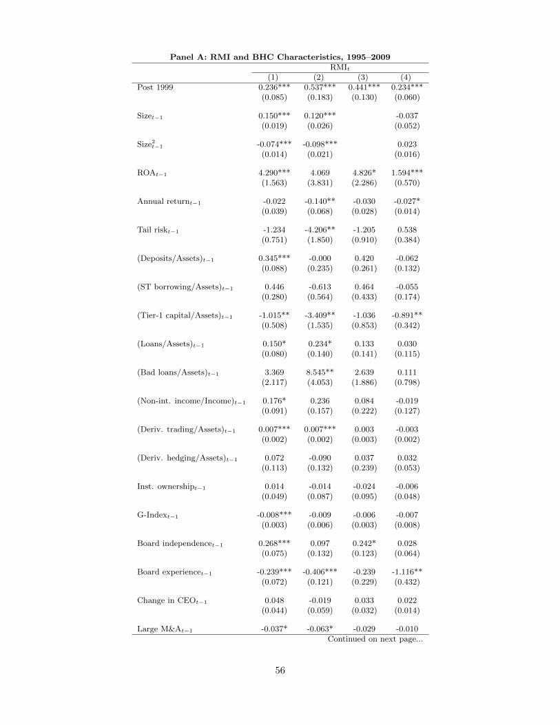
Panel A: RMI and BHC Characteristics, 1995–2009RMIt

(1) (2) (3) (4)Post 1999 0.236*** 0.537*** 0.441*** 0.234***

(0.085) (0.183) (0.130) (0.060)

Sizet−1 0.150*** 0.120*** -0.037(0.019) (0.026) (0.052)

Size2t−1 -0.074*** -0.098*** 0.023(0.014) (0.021) (0.016)

ROAt−1 4.290*** 4.069 4.826* 1.594***(1.563) (3.831) (2.286) (0.570)

Annual returnt−1 -0.022 -0.140** -0.030 -0.027*(0.039) (0.068) (0.028) (0.014)

Tail riskt−1 -1.234 -4.206** -1.205 0.538(0.751) (1.850) (0.910) (0.384)

(Deposits/Assets)t−1 0.345*** -0.000 0.420 -0.062(0.088) (0.235) (0.261) (0.132)

(ST borrowing/Assets)t−1 0.446 -0.613 0.464 -0.055(0.280) (0.564) (0.433) (0.174)

(Tier-1 capital/Assets)t−1 -1.015** -3.409** -1.036 -0.891**(0.508) (1.535) (0.853) (0.342)

(Loans/Assets)t−1 0.150* 0.234* 0.133 0.030(0.080) (0.140) (0.141) (0.115)

(Bad loans/Assets)t−1 3.369 8.545** 2.639 0.111(2.117) (4.053) (1.886) (0.798)

(Non-int. income/Income)t−1 0.176* 0.236 0.084 -0.019(0.091) (0.157) (0.222) (0.127)

(Deriv. trading/Assets)t−1 0.007*** 0.007*** 0.003 -0.003(0.002) (0.002) (0.003) (0.002)

(Deriv. hedging/Assets)t−1 0.072 -0.090 0.037 0.032(0.113) (0.132) (0.239) (0.053)

Inst. ownershipt−1 0.014 -0.014 -0.024 -0.006(0.049) (0.087) (0.095) (0.048)

G-Indext−1 -0.008*** -0.009 -0.006 -0.007(0.003) (0.006) (0.003) (0.008)

Board independencet−1 0.268*** 0.097 0.242* 0.028(0.075) (0.132) (0.123) (0.064)

Board experiencet−1 -0.239*** -0.406*** -0.239 -1.116**(0.072) (0.121) (0.229) (0.432)

Change in CEOt−1 0.048 -0.019 0.033 0.022(0.044) (0.059) (0.032) (0.014)

Large M&At−1 -0.037* -0.063* -0.029 -0.010Continued on next page...

56

Table continued...RMIt

(1) (2) (3) (4)(0.022) (0.036) (0.021) (0.008)

CEO’s deltat−1 -0.873(0.562)

CEO’s vegat−1 0.193***(0.054)

CEO’s tenuret−1 -0.010***(0.003)

Constant 0.110 0.815*** -0.241 0.796***(0.103) (0.276) (0.222) (0.182)

Observations 695 366 695 695R2 0.404 0.438 0.470 0.953Year FE Yes Yes Yes YesSize decile FE No No Yes NoBHC FE No No No Yes

Panel B: Performance during 1998 Crisis and RMI in 1999-2009(1) (2) (3) (4) (5)

RMI ∆RMI ∆RMI1998−00 ∆RMI2000−03 ∆RMI2003−06

High tail risk 1998 -0.075*** -0.009 -0.015 -0.063 -0.001(0.022) (0.006) (0.057) (0.072) (0.046)

Constant 0.283 0.001 0.122 0.330 -0.077(0.221) (0.014) (0.579) (0.602) (0.317)

Observations 570 549 37 48 55R2 0.480 0.270 0.834 0.301 0.357Year FE Yes Yes No No NoSize decile FE Yes Yes Yes Yes YesBHC controls Yes Yes Yes Yes Yes

57

Table

IV:Pre

-crisisRM

Iand

Perform

anceduringth

eCrisisYears

This

table

rep

ort

sth

ere

sult

sof

cross

-sec

tional

regre

ssio

ns

that

exam

ine

whet

her

BH

Cs

wit

hhig

hPre-crisisRMI

(defi

ned

as

the

BH

C’s

aver

ageRMI

over

the

yea

rs2005

and

2006)

fare

db

ette

rduri

ng

the

cris

isyea

rs.

We

esti

mate

the

regre

ssio

n

Yj,t

=α

+β∗

Pre

-cri

sis

RM

I j+

γ∗X

j,2006

+Y

ear

FE

We

confine

this

regre

ssio

nto

the

financi

al

cris

isyea

rs,

2007

and

2008.

Inco

lum

ns

(1)

and

(2),Y

isPrivate

MBS

whic

hden

ote

sth

eto

tal

valu

eof

pri

vate

-lab

elm

ort

gage-

back

edse

curi

ties

(in

$m

illion)

hel

din

both

tradin

gand

inves

tmen

tp

ort

folios.

Inco

lum

n(3

),Y

isDeriv.trading

whic

his

the

gro

ssnoti

onal

am

ount

(in

$billion)

of

der

ivati

ve

contr

act

shel

dfo

rtr

adin

gpurp

ose

s.In

colu

mn

(4),Y

isBadloans/assets

wher

eBadloans

incl

ude

loans

past

due

90

day

sor

more

and

non-a

ccru

al

loans.

Inco

lum

n(5

),Y

isROA

whic

his

the

rati

oof

inco

me

bef

ore

extr

aord

inary

item

sto

ass

ets.

Inco

lum

n(6

),Y

isAnnualreturn

whic

his

buy-a

nd-h

old

retu

rnon

the

BH

C’s

stock

over

the

cale

ndar

yea

r.In

colu

mn

(7),Y

isTailrisk

whic

his

the

neg

ati

ve

of

the

aver

age

retu

rnon

the

BH

C’s

stock

duri

ng

the

5%

wors

tre

turn

day

sfo

rth

eB

HC

’sst

ock

over

the

yea

r.D

efinit

ions

of

all

oth

erva

riable

sare

list

edin

App

endix

B.

We

contr

ol

the

regre

ssio

nfo

rB

HC

chara

cter

isti

csin

the

yea

r2006,

and

incl

ude

yea

rfixed

effec

tsin

all

spec

ifica

tions.

Sta

ndard

erro

rs(r

eport

edin

pare

nth

eses

)are

robust

tohet

erosk

edast

icit

yand

are

clust

ered

at

the

BH

Cle

vel

.W

euse

the

sym

bols

***,

**,

and

*to

den

ote

stati

stic

al

signifi

cance

at

the

1%

,5%

,and

10%

level

s,re

spec

tivel

y.

58

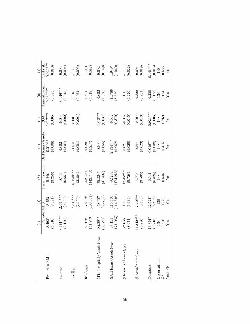
(1)

(2)

(3)

(4)

(5)

(6)

(7)

Pri

vate

MB

SD

eriv

.tr

adin

gB

ad

loans/

Ass

ets

RO

AA

nnual

retu

rnT

ail

risk

Pre

-cri

sis

RM

I-8

.492*

-3.3

55

5.2

46

-0.0

19**

0.0

17***

0.3

30***

-0.0

29***

(4.3

40)

(2.5

91)

(3.2

59)

(0.0

08)

(0.0

05)

(0.0

83)

(0.0

10)

Siz

e 2006

8.1

71***

2.3

30***

-0.5

69

0.0

02

-0.0

03

-0.1

40***

0.0

04

(2.1

20)

(0.6

33)

(0.6

61)

(0.0

01)

(0.0

02)

(0.0

45)

(0.0

04)

Siz

e2 2006

7.7

99***

10.3

40***

-0.0

01

0.0

01

0.0

48

-0.0

03

(2.1

56)

(2.3

04)

(0.0

01)

(0.0

01)

(0.0

34)

(0.0

03)

RO

A2006

239.1

26*

176.4

56

-228.2

64

0.0

29

1.3

01

-0.2

01

(141.8

79)

(108.0

01)

(142.7

78)

(0.2

17)

(4.5

48)

(0.5

17)

(Tie

r1ca

pit

al/

Ass

ets)

2006

-85.2

91*

-58.1

27

75.8

24*

-0.0

04

0.3

13***

-0.6

02

0.0

02

(50.7

21)

(36.7

32)

(41.4

37)

(0.0

55)

(0.0

37)

(1.3

36)

(0.1

49)

(Bad

loans/

Ass

ets)

2006

67.1

51

115.5

40

-92.7

99

2.9

34***

-0.5

62

-11.7

89

1.9

49*

(171.0

65)

(114.8

16)

(174.2

55)

(0.9

62)

(0.3

79)

(8.5

59)

(1.0

40)

(Dep

osi

ts/A

sset

s)2006

-2.6

55

1.3

58

12.4

52**

0.0

21

-0.0

07

0.1

60

-0.0

33

(8.0

54)

(6.3

39)

(5.7

26)

(0.0

25)

(0.0

10)

(0.2

29)

(0.0

22)

(Loans/

Ass

ets)

2006

-11.3

42***

-7.7

56**

-5.0

35

-0.0

16

-0.0

14

-0.3

22

0.0

04

(4.2

80)

(3.3

36)

(3.5

03)

(0.0

23)

(0.0

10)

(0.2

01)

(0.0

19)

Const

ant

18.8

54*

12.5

21*

-6.6

41

0.0

16**

-0.0

21***

-0.2

30

0.1

48***

(9.7

48)

(6.8

05)

(5.8

25)

(0.0

08)

(0.0

05)

(0.1

73)

(0.0

16)

Obse

rvati

ons

138

138

138

138

138

138

138

R2

0.5

56

0.7

20

0.6

46

0.4

15

0.7

69

0.1

74

0.6

66

Yea

rF

EY

esY

esY

esY

esY

esY

esY

es

59

Table V: Relationship between Tail Risk and RMI

This table reports the results of panel regressions that examine the relationship between a BHCs’ Tail risk

and RMI. We estimate the regression

Tail riskj,t = α+ β ∗ RMIj,t−1 + γ ∗Xj,t−1 + BHC or Size Decile FE + Year FE

We estimate the regression on a panel that has one observation for each BHC-year combination, and spans the

time period 1995 to 2010. Tail risk is defined as the negative of the average return on the BHC’s stock over

the 5% worst return days for the BHC’s stock during the year. All other variables are defined in Appendix

B. We include year fixed effects in all specifications, size decile fixed effects in column (4), and BHC fixed

effects in column (5). Standard errors (reported in parentheses) are robust to heteroskedasticity and are

clustered at the level of the BHC. We use the symbols ***, **, and * to denote statistical significance at the

1%, 5%, and 10% levels, respectively.

Tail riskt

(1) (2) (3) (4) (5)

RMIt−1 -0.009** -0.008** -0.009** -0.010** -0.022**

(0.004) (0.004) (0.004) (0.004) (0.010)

Sizet−1 0.001 0.000 0.003 0.004

(0.001) (0.002) (0.002) (0.006)

Size2t−1 0.002* 0.003*** 0.004** 0.007***

(0.001) (0.001) (0.002) (0.002)

ROAt−1 -0.688*** -0.760*** -1.266*** -0.695*** -0.747**

(0.187) (0.203) (0.177) (0.208) (0.283)

Annual returnt−1 -0.010*** -0.009*** -0.011** -0.009*** -0.007***

(0.003) (0.003) (0.005) (0.003) (0.003)

(Deposits/Assets)t−1 -0.006 -0.009 0.023 -0.014 0.040**

(0.010) (0.011) (0.015) (0.012) (0.020)

(ST borrowing/Assets)t−1 0.017 0.016 0.007 0.008 0.037

(0.019) (0.019) (0.032) (0.019) (0.027)

(Tier-1 capital/Assets)t−1 0.164*** 0.192*** 0.058 0.164*** 0.226***

(0.047) (0.052) (0.103) (0.054) (0.079)

(Loans/Assets)t−1 -0.012 -0.021*** -0.022** -0.024*** -0.031

(0.007) (0.006) (0.011) (0.006) (0.021)

(Bad loans/Assets)t−1 1.061*** 1.156*** 1.587*** 1.125*** 0.906**

(0.250) (0.267) (0.505) (0.261) (0.423)

(Non-int. income/Income)t−1 -0.005 -0.020* -0.010 -0.023** -0.048**

(0.010) (0.011) (0.010) (0.011) (0.020)

(Deriv. trading/Assets)t−1 -0.000*** -0.000*** 0.000 0.000

Continued on next page...

60

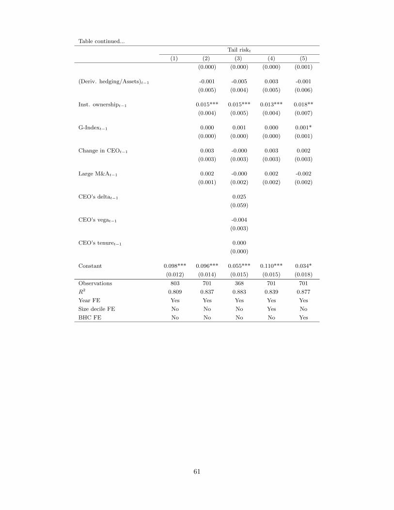
Table continued...

Tail riskt

(1) (2) (3) (4) (5)

(0.000) (0.000) (0.000) (0.001)

(Deriv. hedging/Assets)t−1 -0.001 -0.005 0.003 -0.001

(0.005) (0.004) (0.005) (0.006)

Inst. ownershipt−1 0.015*** 0.015*** 0.013*** 0.018**

(0.004) (0.005) (0.004) (0.007)

G-Indext−1 0.000 0.001 0.000 0.001*

(0.000) (0.000) (0.000) (0.001)

Change in CEOt−1 0.003 -0.000 0.003 0.002

(0.003) (0.003) (0.003) (0.003)

Large M&At−1 0.002 -0.000 0.002 -0.002

(0.001) (0.002) (0.002) (0.002)

CEO’s deltat−1 0.025

(0.059)

CEO’s vegat−1 -0.004

(0.003)

CEO’s tenuret−1 0.000

(0.000)

Constant 0.098*** 0.096*** 0.055*** 0.110*** 0.034*

(0.012) (0.014) (0.015) (0.015) (0.018)

Observations 803 701 368 701 701

R2 0.809 0.837 0.883 0.839 0.877

Year FE Yes Yes Yes Yes Yes

Size decile FE No No No Yes No

BHC FE No No No No Yes

61

Table

VI:

Relationsh

ipbetw

een

RM

Iand

Perform

ance

This

table

rep

ort

sth

ere

sult

sof

panel

regre

ssio

ns

inves

tigati

ng

the

rela

tionsh

ipb

etw

een

aB

HC

’sp

erfo

rmance

and

itsRMI.

We

esti

mate

the

follow

ing

regre

ssio

n:

Yj,t

=α

+β∗

RM

I j,t−1

+γ∗X

j,t−1

+B

HC

or

Siz

eD

ecile

FE

+Y

ear

FE

Inth

isre

gre

ssio

n,Y

isa

mea

sure

of

the

BH

C’s

op

erati

ng

per

form

ance

(in

colu

mns

(1)

thro

ugh

(3))

or

stock

retu

rnp

erfo

rmance

(in

colu

mns

(4)

thro

ugh

(9))

.

We

mea

sure

op

erati

ng

per

form

ance

usi

ngROA

whic

his

the

rati

oof

inco

me

bef

ore

extr

aord

inary

item

sto

ass

ets.

We

mea

sure

stock

retu

rnp

erfo

rmance

usi

ng

the

follow

ing

vari

able

s:Annualreturn

,w

hic

his

the

buy-a

nd-h

old

retu

rnon

the

BH

C’s

stock

over

the

cale

ndar

yea

r;andAbn

orm

alreturn

whic

his

the

diff

eren

ce

bet

wee

nth

eact

ualAnnualreturn

and

the

exp

ecte

dre

turn

from

am

ark

etm

odel

,w

her

eth

em

ark

etm

odel

ises

tim

ate

dby

regre

ssin

gdaily

retu

rns

on

the

BH

C’s

stock

ver

sus

aco

nst

ant

and

daily

retu

rns

on

the

S&

P500

over

the

past

thre

eca

lendar

yea

rs.Crisisyear

isa

dum

my

vari

able

that

iden

tifies

the

financi

al

cris

is

yea

rs,

2007

and

2008.

We

als

oco

ntr

ol

the

regre

ssio

ns

for

the

follow

ing

BH

Cch

ara

cter

isti

cs,

but

do

not

rep

ort

the

coeffi

cien

tsin

ord

erto

conse

rve

space

:Annual

return

t−1

(in

colu

mns

(1)

thro

ugh

(3)

only

),ROA

t−1

(in

colu

mns

(4)

thro

ugh

(9)

only

),(D

eposits/Assets)

t−1,(T

ier-1capital/Assets)

t−1,(L

oans/Assets)

t−1,

(Badloans/Assets)

t−1,

andNon-int.

income/Incomet−

1.

All

vari

able

sare

defi

ned

inA

pp

endix

B.

We

incl

ude

yea

rfixed

effec

tsand

eith

ersi

zedec

ile

fixed

effec

ts

or

BH

Cfixed

effec

tsin

all

spec

ifica

tions.

Sta

ndard

erro

rs(r

eport

edin

pare

nth

eses

)are

robust

tohet

erosk

edast

icit

yand

are

clust

ered

at

the

BH

Cle

vel

.W

euse

the

sym

bols

***,

**,

and

*to

den

ote

stati

stic

al

signifi

cance

at

the

1%

,5%

,and

10%

level

s,re

spec

tivel

y.

62

RO

At

Annual

retu

rnt

Abnorm

al

retu

rnt

(1)

(2)

(3)

(4)

(5)

(6)

(7)

(8)

(9)

RM

I t−1

0.0

06**

0.0

07*

0.0

72**

0.0

37

0.0

75**

0.0

74

(0.0

02)

(0.0

04)

(0.0

32)

(0.1

21)

(0.0

32)

(0.1

15)

Cri

sis

yea

r0.0

08***

-0.2

95***

-0.7

31***

(0.0

02)

(0.0

36)

(0.0

41)

RM

I t−1*C

risi

syea

r0.0

10***

0.1

57**

0.1

47**

(0.0

04)

(0.0

73)

(0.0

72)

RM

I t−1*(1

-Cri

sis

yea

r)0.0

05*

0.0

48

0.0

54

(0.0

02)

(0.0

35)

(0.0

35)

Const

ant

-0.0

17***

-0.0

14**

-0.0

02

0.2

24***

0.2

63***

3.3

67***

0.6

45***

0.6

87***

2.9

63***

(0.0

06)

(0.0

06)

(0.0

27)

(0.0

63)

(0.0

67)

(0.6

71)

(0.0

69)

(0.0

71)

(0.7

07)

Obse

rvati

ons

805

805

805

804

804

804

803

803

803

R2

0.7

26

0.7

28

0.8

02

0.5

23

0.5

25

0.5

65

0.5

72

0.5

73

0.6

05

Yea

rF

EY

esY

esY

esY

esY

esY

esY

esY

esY

es

Siz

edec

ile

FE

Yes

Yes

No

Yes

Yes

No

Yes

Yes

No

BH

CF

EN

oN

oY

esN

oN

oY

esN

oN

oY

es

BH

Cco

ntr

ols

Yes

Yes

Yes

Yes

Yes

Yes

Yes

Yes

Yes

63

Table VII: Instrumental-Variables Regressions

Panel A reports the results of instrumental-variables regressions that examine whether BHCs with high

Pre-crisis RMI fared better during the crisis years. We instrument for each BHC’s Pre-crisis RMI using

its Comparable ∆RMI1998−00, which is defined as the average increase in RMI over the period 1998 to 2000

for all other BHCs (i.e., excluding the BHC itself) in the size decile to which the BHC belonged in 1998.

The regressions are estimated using the two-staged least squares (2SLS) estimator, and are confined to the

crisis years, 2007 and 2008. The results of the first-stage regression are presented in column (1), whereas

the results of the second-stage regressions are presented in columns (2) through (4). We control both the

first- and second- stage regressions for the following BHC characteristics, but do not report these coefficients

in order to conserve space: Size2006, Size22006, ROA2006, (Deposits/Assets)2006, (Tier-1 capital/Assets)2006,

(Loans/Assets)2006, and (Bad loans/Assets)2006. Definitions of variables are listed in Appendix B. We

include year fixed effects in all specifications. Standard errors (reported in parentheses) are robust to

heteroskedasticity and are clustered at the BHC level. We use the symbols ***, **, and * to denote

statistical significance at the 1%, 5%, and 10% levels, respectively.

Panel B reports the results of an instrumental-variables panel regression that examines the relationship be-

tween BHCs’ Tail risk t and RMI t−1. We instrument for each BHC’s RMI t−1 using its Comparable BHCs’

∆RMI1998−00, which is defined as the average increase in RMI over the period 1998-2000 for all other BHCs

(i.e., excluding the BHC itself) in the size decile to which the BHC belonged in 1998. The regressions

are estimated using the two-staged least squares (2SLS) estimator. The results of the first- and second-

stage regressions are presented in columns (1) and (2), respectively. We control both the first- and second-

stage regressions for the following BHC characteristics, but do not report these coefficients in order to con-

serve space: Sizet−1, Size2t−1, Annual returnt−1, ROAt−1, (Deposits/Assets)t−1, (Tier-1 capital/Assets)t−1,

(Loans/Assets)t−1, (Bad loans/Assets)t−1, and Non-int. income/Incomet−1. We estimate the regressions

on a panel that has one observation for each BHC-year combination, and spans the time period 2001 to

2010. We include year fixed effects in the regression. Standard errors (reported in parentheses) are robust

to heteroskedasticity, and are clustered at the BHC level. We use the symbols ***, **, and * to denote

statistical significance at the 1%, 5%, and 10% levels, respectively.

Panel A: Pre-crisis RMI and Performance During Crisis Years

(1) (2) (3) (4)

RMI Pre-Crisis ROA Annual Return Tail Risk

Pre-crisis RMI 0.018* 0.582** -0.049*

(0.010) (0.271) (0.027)

Comparable BHCs’ ∆RMI1998−00 1.603***

(0.474)

Constant 0.578** -0.008 -0.583* 0.158***

(0.259) (0.010) (0.326) (0.027)

Observations 116 116 116 116

R2 0.428 0.348 0.146 0.699

F-stat (p-value) of excluded instrument 12.83 (0.0005)

Year FE Yes Yes Yes Yes

BHC controls Yes Yes Yes Yes

64

Panel B: Relationship between Tail risk t and RMI t−1, 2001–2010

(1) (2)

RMIt−1 Tail Riskt

RMIt−1 -0.021*

(0.012)

Comparable BHCs’ ∆RMI1998−00 1.736***

(0.571)

Constant 0.518* 0.097***

(0.291) (0.013)

Observations 524 524

R2 0.420 0.840

F-stat (p-value) of excluded instrument 9.24 (0.0035)

Year FE Yes Yes

BHC controls Yes Yes

65

Table VIII: Dynamic Panel GMM Estimation for the Relationship between Tail Risk and

RMI

In this table, we report the results of the Arellano and Bond (1991) dynamic panel GMM estimator to

investigate the relationship between Tail risk t and RMI t−1. The model we estimate is

Tail riskj,t = α+ β ∗ RMIj,t−1 + κ1Tail riskj,t−1 + κ2Tail riskj,t−2 + γ ∗Xj,t−1 + ηi + εit

The model employs two lags of Tail risk as regressor variables; i.e., BHC characteristics that are lagged

three periods or more are available for use as exogenous instruments. Apart from the variables reported

below, we control the model for the following BHC characteristics, but do not report the coefficients in

order to conserve space: Sizet−1, Size2t−1, Annual returnt−1, ROAt−1, (Deposits/Assets)t−1, (Tier-1 capi-

tal/Assets)t−1, (Loans/Assets)t−1, (Bad loans/Assets)t−1, Non-int. income/Incomet−1, Inst. ownershipt−1,

G-Index t−1, (Deriv. trading/Assets)t−1, (Deriv. hedging/Assets)t−1, CEO’s deltat−1, CEO’s vegat−1,

Change in CEOt−1, and Large M&At−1. Variable definitions are in Appendix B. Standard errors are

reported in parentheses. We use the symbols ***, **, and * to denote statistical significance at the 1%, 5%,

and 10% levels, respectively.

Tail riskt

RMIt−1 -0.097***

(0.014)

Tail riskt−1 0.196**

(0.092)

Tail riskt−2 -0.335***

(0.067)

Constant 0.189***

(0.027)

Observations 338

Sargan χ2 37.184

Sargan p-value 1.000

BHC Controls Yes

66

Notes

1Comments from his special address delivered at the 44th annual Conference on Bank Structure and

Competition, held at the Federal Reserve of Chicago in May 2008.

2Stulz (2008) characterizes a failure of risk management as one of the following: failure to identify or

correctly measure risks, failure to communicate risk exposures to the top management, and failure to monitor

or manage risks adequately.

3The Senior Supervisors Group (SSG) is a group of supervisory agencies from France, Germany, Switzer-

land, the United Kingdom, and the United States.

4The inability of risk managers to restrain bank executives is highlighted by the experience of David

Andrukonis, a risk manager at Freddie Mac, who tried to alert his senior management to the risks in

subprime and Alt-A loans, but was unable to restrain them (see Calomiris (2008)).

5In this regard, our paper is related to the literature that examines whether executive compensation may

have contributed to the risk-taking behavior of financial institutions in the lead up to the financial crisis.

Fahlenbrach and Stulz (2011) find that CEOs with higher option/ cash bonus compensation did not perform

worse during the crisis. On the other hand, Cheng, Hong, and Scheinkman (2011) find a correlation between

total executive compensation, controlling for firm size, and risk measures.

6Consistent with hedging theories, Purnanandam (2007) shows that banks that face a higher probability

of financial distress manage their interest rate risk more aggressively, both by using derivatives and by

adopting conservative asset-liability management policies.

7We also create two additional risk measures, Downside risk and Aggregate risk ; the results using these

risk measures are shown in the internet appendix. The Downside risk measure is defined as the mean implied

volatility estimated using put options written on the BHC’s stock (Bali and Hovakimian (2009), Cremers

and Weinbaum (2010) and Xing, Zhang, and Zhao (2010)). We obtain implied volatilities estimated from

option prices from the OptionMetrics database. Aggregate risk is defined as the standard deviation of the

BHC’s weekly return over the calendar year (see Demsetz, Saidenberg, and Strahan (1997) and Laeven and

Levine (2009)).

8In some of the smaller BHCs that are mainly oriented towards retail banking, the Chief Lending Officer

or the Chief Credit Officer may be the official in charge of risk management. To ensure that we are not

missing out on these alternative designations, we treat them on par with Chief Risk Officer while coding

these variables.

9We exclude the CRO’s stock and option awards while computing the CRO centrality measure because

67

it could be argued that a CRO with a high proportion of variable compensation will not have the incentives

to restrain the risk-taking tendencies of executives and traders. We thank an anonymous referee for this

suggestion.

10The reasoning behind using the CFO’s compensation is that, in BHCs that do not have a designated

CRO, the CFO is most likely in charge of risk management.

11We recognize that this procedure may potentially generate inconsistent factor loadings across the years

in our sample. To investigate this potential problem, and to check the stability and robustness of our

factors, we also use a principal component analysis where the loadings are determined over the entire sample

period. The correlation between the loadings of the two principal components (one where the analysis is

done annually and the other done over the entire sample period) is very high for all 6 factors (it ranges

from 81% to 90%), giving us comfort about the stability of our analysis independent of how loadings are

determined. Moreover, we obtain very similar results when we employ an alternative RMI where the factor

loadings are measured over the entire sample period (see Table IA.III in the internet appendix).

12We obtain qualitatively similar results when we use the buy-and-hold return from August-December

1998 to identify the BHCs with the worst performance during the 1998 crisis. As Fahlenbrach, Prilmeier,

and Stulz (2011) note, the 1998 crisis began in August 1998 but was fairly short-lived. Many bank stocks

plummeted initially but then also recovered somewhat subsequently. Therefore, the August-December return

is a reasonable metric to measure how BHCs fared during the 1998 crisis.

13We obtain qualitatively similar results when we use lagged BHC characteristics, instead of 2006 charac-

teristics, as control variables.

14However, the findings in the empirical literature in this regard are somewhat mixed. Examining bank

behavior during the period 1992–2002, Mehran and Rosenberg (2007) find that equity volatility and asset

volatility of banks increase as their CEO stock option holdings increase. However, examining the behavior

of banks during the crisis period, Fahlenbrach and Stulz (2011) find that option compensation did not have

an adverse impact on bank performance.

15Specifically, the model that we estimate is Tail riskj,t = α+ β ∗RMIj,t−1 + γ ∗Xj,t−1 + µj + µt + ej,t,

where the error term ej,t is modeled as ej,t = ρ ∗ ej,t−1 + zj,t.

16The fixed effects estimation is based on deviations of variables from their mean values for the BHC,

which may introduce look-ahead bias because the mean value is computed over the entire sample period.

The advantage of the first-difference specification is that it examines deviations of variables from their values

in the previous period, and hence, is not subject to look-ahead bias.

17In the context of large financial institutions, it is particularly difficult to distinguish between idiosyncratic

and systematic risk.

68

18The first-stage regressions are the same for all IV regressions in Panel A. Therefore, to conserve space,

we only report the first-stage regression once.

19With one exogenous instrument, the first-stage F−statistic must exceed 8.96 for the 2-SLS inference to

be reliable (see Table 1 in Stock, Wright, and Yogo (2002)).

20Again, the F−statistic of 9.24 is higher than the threshold of 8.96 specified in Stock et al. (2002),

despite the fact that we have a small sample, and that we cluster standard errors at the BHC level (as we

should).

21We use a simple average to define Quality of oversight because it is objectively difficult to figure out the

relative importance of the Risk committee experience and Active risk committee. We obtain qualitatively

similar results when we estimate the regression with all the six RMI components as separate regressor

variables, instead of combining them into two categories. However, the interpretation of results is more

meaningful with CRO centrality and Quality of oversight as the independent variables.

69