Offshore Windfarm Design Optimization using Dynamic Rating ...

General rights Copyright and moral rights for the publications made accessible in the public portal are retained by the authors and/or other copyright owners and it is a condition of accessing publications that users recognise and abide by the legal requirements associated with these rights.

Users may download and print one copy of any publication from the public portal for the purpose of private study or research.

You may not further distribute the material or use it for any profit-making activity or commercial gain

You may freely distribute the URL identifying the publication in the public portal If you believe that this document breaches copyright please contact us providing details, and we will remove access to the work immediately and investigate your claim.

Downloaded from orbit.dtu.dk on: Dec 15, 2021

Offshore Windfarm Design Optimization using Dynamic Rating for TransmissionComponents

Kazmi, Syed Hamza Hasan; Viafora, Nicola; Sørensen, Troels; Olesen, Thomas Herskind; Pal, BikashChandra; Holbøll, Joachim

Published in:IEEE Transactions on Power Systems

Link to article, DOI:10.1109/TPWRS.2021.3118278

Publication date:2021

Document VersionPeer reviewed version

Link back to DTU Orbit

Citation (APA):Kazmi, S. H. H., Viafora, N., Sørensen, T., Olesen, T. H., Pal, B. C., & Holbøll, J. (Accepted/In press). OffshoreWindfarm Design Optimization using Dynamic Rating for Transmission Components. IEEE Transactions onPower Systems. https://doi.org/10.1109/TPWRS.2021.3118278

https://doi.org/10.1109/TPWRS.2021.3118278

https://orbit.dtu.dk/en/publications/443da23c-ae2f-4000-984e-2b9bb913c4e1

https://doi.org/10.1109/TPWRS.2021.3118278

0885-8950 (c) 2021 IEEE. Personal use is permitted, but republication/redistribution requires IEEE permission. See http://www.ieee.org/publications_standards/publications/rights/index.html for more information.

This article has been accepted for publication in a future issue of this journal, but has not been fully edited. Content may change prior to final publication. Citation information: DOI 10.1109/TPWRS.2021.3118278, IEEETransactions on Power Systems

SUBMITTED TO IEEE TRANSACTIONS ON POWER SYSTEMS, SEP 2021 1

Offshore Windfarm Design Optimization usingDynamic Rating for Transmission Components

Syed Hamza H. Kazmi, Student Member, IEEE, Nicola Viafora, Student Member, IEEE, Troels S. Sørensen,Thomas H. Olesen, Member, IEEE, Bikash C. Pal, Fellow, IEEE, Joachim Holbøll, Sr. Member, IEEE

Abstract—The foreseen development of large-scale OffshoreWindfarms (OWFs) further from the shore dictates that theOWF transmission system must be optimally designed basedon Dynamic Thermal Rating (DTR) in order to fully utilizethe intermittent nature of the wind and to keep the offshorewind cost-competitive. In this paper, a comprehensive, DTR-based, two-stage stochastic model is presented, which has beendeveloped for investment decision support for OWF size andHVAC transmission systems. Complex DTR models for all thecritical HV components are made fit for the mixed-integer linearprogramming problem, while accounting for the stochasticity inwind generation and component availability. The main decisionsincorporate the discrete size of OWFs, HV subsea export cablecross-sections and ratings for transformers and shunt reactors.For validation, an actual testcase OWF off the east coast of UKhas been used. Results indicate that DTR-based iterative design ofOWF and its transmission components can significantly improvethe business case, even though transmission efficiency and energydelivered are not maximum for the optimal design case.

Index Terms—Dynamic thermal rating, offshore windfarms,stochastic design optimization, HVAC transmission, reliability.

NOMENCLATURE

A. Sets (Indices) and Components (Superscipts)

j ∈ J Set of tangent lines for losses approximationk ∈ K Set of candidate design cases (Opt. case: kopt)l ∈ L Set of tangent lines for ageing approximations ∈ S Set of scenariost ∈ T Set of hours in each yeary ∈ Y Set of years in windfarm lifetime ΠWF [yr]base, opt Base and optimal design casestur Wind Turbines (WTs)c Cables and circuitstrf TransformersSR Shunt Reactors

B. Parameters and Inputs

ak, bk Thermal coefficients for cables and transformersAwt,s A

ct,s OWF & transmission circuit availability

ck Cost of components [e/unit, e/km, e/tonne]Cx,k Csoil Thermal capacitance for cable & soil [J/mC]gk Cost coefficients for cablesIcQ k Reactive component of cable current [A]Lc Length of subsea export cable [m]mk Mass of relevant components [tonne]n Number of componentspj,l qj,l slope and intercepts for linear approx.Pwt,s OWF power generation [pu]

rk Resistance of components at temp. limits [Ω]Sk Rated power of components [MVA, MW, MVAr]Tx,k Tsoil Thermal resistance for cable & soil [mC/W]Wd,kWnl,k Dielectric & noload loss in cables & trafos [W]i Discount rate for NPV calculation [pu]γ Power purchase agreement price [e/MWh]Λ, Υ Failure & repair rates for components [hr−1]λcs λ

ca Loss factors for cable screen and armouring [pu]

ϑambt,s ϑsea

t,s Ambient and seabed temperatures [C]

C. Decision variables

C0 Investment costs = f(ntur, Cfix, Cexp

k

)[Me]

It,s IP t,s Component load current apparent and active [A]ntur Number of wind turbinesP gent,s Hourly power generated by the OWF [MW]P cutt,s P

injt,s Hourly power curtailed & injected to grid [MW]

Rs Total revenue over OWF lifetime [Me]Wt,s Losses in components [W]ϑservt,s ϑc

t,s Cable serving & cond. temp. rise over ϑsea [C]ϑtopt,s ϑ

hstt,s Transformer top oil & hot spot temp. [C]

λy,s Transformer loss of life - yearly (LL) [hr]

I. INTRODUCTION

The growth in offshore wind has been expedited exponen-tially by decreasing the Levelised Cost Of Energy (LCOE)from 180 to less than 40 e

MWh over the last decade [1]. Thishas resulted in intense price competition in the markets and hasprompted developers and manufacturers alike to optimize theentire value chain [2]. The electrical infrastructure for OffshoreWind Farms (OWFs) usually consist of two systems: thecollection system interconnecting Wind Turbines (WTs) withOffshore Substations (OSSs) and the HV transmission systemresponsible for energy transfer from OSS to the onshorestation. Conventionally, the number of WTs and ratings ofHV transmission components are coupled iteratively duringthe OWF design phase [3]. With the development of large-scale OWFs further from the shore, the potential to optimizethe transmission components escalates as well. Utilization ofDynamic Thermal Rating (DTR) for the dimensioning of thesecomponents and optimization of the OWF size based on thisdesign can drive down the LCOE further.

Over the years, several publications [3]–[14] have been pre-sented for OWF design optimization addressing the electricalinfrastructure’s efficiency and costs related to investment andoperation. A vast majority of these publications focus on thecollection system along by performing layout and array cable

Authorized licensed use limited to: Danmarks Tekniske Informationscenter. Downloaded on October 07,2021 at 06:38:53 UTC from IEEE Xplore. Restrictions apply.




routing optimization [4]–[8]. On the other hand, only a handfulof research has been done on the OWF transmission system,with most publications focused only on the optimal design ofHVAC submarine cables without the application of DTR [3],[9]–[11]. The potential of cost reduction by optimization ofremaining components [15] and by employing DTR on theentire system altogether to resolve any unintentional systembottlenecks is completely unexplored [16], [17]. This paperuniquely targets the optimized design of the entire OWFtransmission system by using coordinated DTR of the majorHV components.

In contrast to Static Thermal Rating (STR), accurate andcomputationally efficient thermal models are needed for DTR-based design. Empirically derived Thermo-Electric Equivalent(TEE) models fit this profile to a large extent. For oil-filledcomponents, the first-order differential models from [18], [19]can be made fit for linear estimation [16], [20] for intermittentdynamic offshore wind generation [15]. Contrarily, single-core equivalent TEE models for three-core HVAC subseacables in [21]–[23] are complicated to design [24], but canbe transformed to account for effective losses in long cables[25], [26] and backfill soil’s thermal parameter variation [27].

OWF transmission system’s contingency and reliability as-sessment is a critical step during the design phase owingto longer repair times and increasing capacity factors [5],[17]. The stochastic nature of system’s availability can beaddressed by using probability-based methods relying onanalytical techniques [28] or Monte Carlo simulations [5],[10], [29]. The computational stress of these techniques fordesign optimization is a challenge that needs to be resolved.Furthermore, the inexact nature of the latter methodology ofreliability modeling is settled by using the scenario generationprinciple.

In this paper, a unique comprehensive model for investmentdecision support for OWF size and HVAC-based transmissionsystem design is proposed. This two-stage stochastic modeluses DTR for optimal utilization of HV components over thewindfarm lifetime and has three fundamental characteristics:business case assessment (investment cost and weighted rev-enue loss due to energy not served), reliability of operationand transmission efficiency. Besides the investment decisionparameters, the model determines the optimal OWF size andoptimal design case incl. ratings of subsea export cables, powertransformers and shunt reactors. The four major contributionsof this work include: a) Development and validation of asimplified TEE model for subsea cables which is fit for linearoptimization. b) Employment of linearized dynamic lifetimeutilization of transformer for OWF design. c) Inclusion ofcontingency scenarios for OWF export system based on MonteCarlo simulations. d) Proposal of a two-stage stochastic modelfor business-case optimization of OWF design by using DTRon the entire HV transmission network accounting for load-dependent losses, curtailment and reliability over OWF life-time.

Remaining paper is structured as follows. Overview of themethodology is given in Sec. II, followed by presentation andvalidation of DTR models for the relevant transmission com-ponents in Sec. III. The novelty of the proposed optimization

methodology is elaborated in detail in Sec. IV. Sec. V presentsthe test case OWF, its design cases and economic assumptions,while the relevance of the proposed problem is demonstratedin Sec. VI. Finally, the paper is concluded in Sec. VII.

II. OVERVIEW OF THE PROPOSED FRAMEWORK

The novel methodology proposed in this paper follows fourbasic steps, as shown in Fig. 1. The first two steps generateinputs for the optimization problem. First of all, dependingon windfarm topology and other predefined factors, a num-ber of potential design cases K with unique combinationsof transformer and cable ratings are preselected. Therefore,component costs, ratings and thermal parameters for eachdesign case are readily available for the optimization frame-work. Secondly, in order to ensure the reliability of design,stochasticity of wind speed and temporal availability of WTsand transmission system is accounted for through scenariogeneration. A set of S scenarios for hourly wind powergeneration profile [pu] over windfarm lifetime are generated byperforming ARIMA-based trend analysis of long-term historicsite data (incl. windspeed and direction profiles). Possiblefailures and contingency conditions are also pre-simulated inthis step which are based on component reliability indices.

In step 3, for each design case the optimization problemmaximizes the business case over OWF lifetime and deter-mines the respective optimal number of wind turbines ntur. Thetwo-level problem deals with operational scenarios and hourlyconstraints (incl. component loading, temperatures, ageing,losses and possible curtailment) at the lower level; whereas, theupper level manages yearly energy injection and componentlifetime utilization over the windfarm lifetime. Finally, thecomponent ratings and optimal ntur for the best design casekopt resulting in maximum NPV are chosen in step 4.

Power BalanceLossesCurtailment

Thermal & AgeingAnalysis

(STR/DTR)

Select optimaldesign

case with max NPV

Preselectcandidate

design cases

Stage 2 Hourly operational constraints

Stage 1 Yearly constraints

Energy Injection

Comp. LifetimeUtilization

Objective Function

Step 3 - Run opt. problem over WF Lifetime for all design cases individually

RatingsParametersCosts

Step 1

Step 4

GenerateScenarios

Step 2

Power gen.Amb. TempComponentAvailability

No. of WTGsNPV

Fig. 1. Proposed framework for the novel optimization strategy

III. DYNAMIC RATING MODELS OF HV COMPONENTS

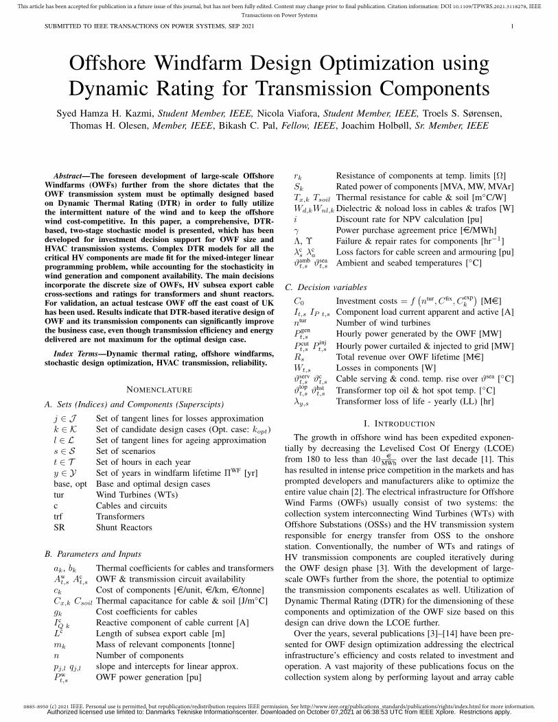
As shown in Fig. 2, the HVAC OWF export system isequipped with nc interlinked parallel circuits consisting of 3-core subsea cables, two parallel transformers in the OSS, withoptional shunt reactors in the middle for long cables.





Fig. 2. Typical layout for a large OWF HV export system with three circuits

A. Cable Thermal Modeling

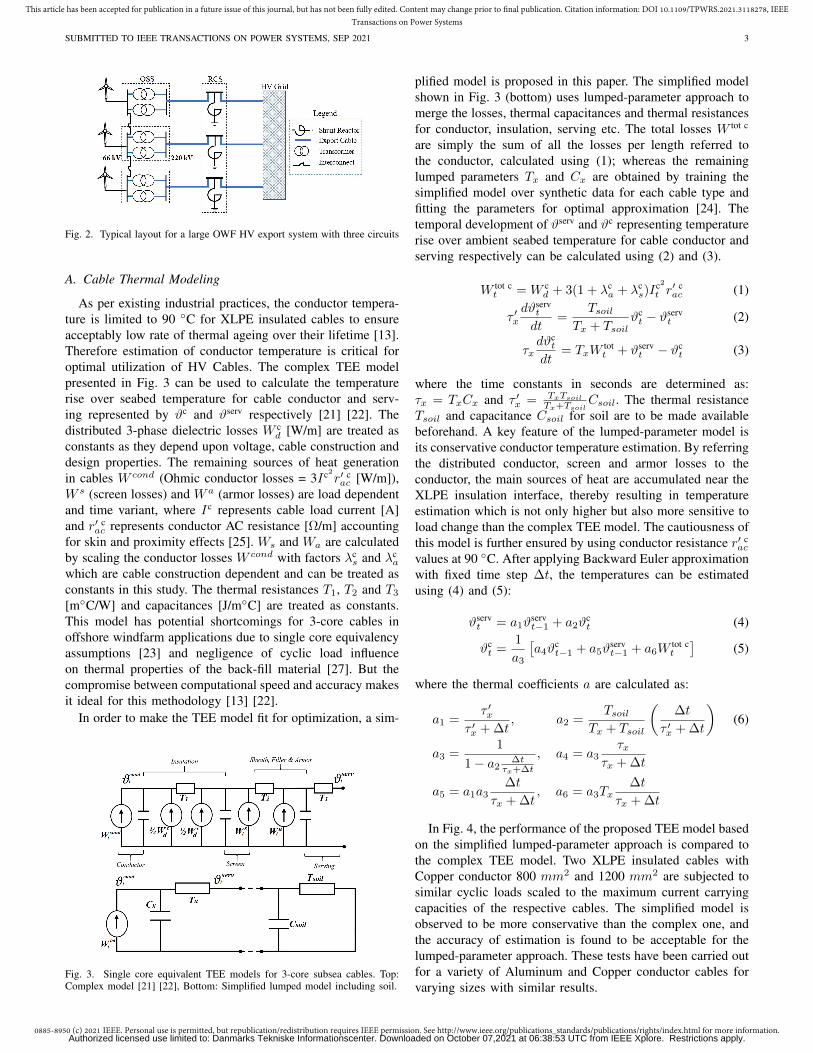
As per existing industrial practices, the conductor tempera-ture is limited to 90 C for XLPE insulated cables to ensureacceptably low rate of thermal ageing over their lifetime [13].Therefore estimation of conductor temperature is critical foroptimal utilization of HV Cables. The complex TEE modelpresented in Fig. 3 can be used to calculate the temperaturerise over seabed temperature for cable conductor and serv-ing represented by ϑc and ϑserv respectively [21] [22]. Thedistributed 3-phase dielectric losses W c

d [W/m] are treated asconstants as they depend upon voltage, cable construction anddesign properties. The remaining sources of heat generationin cables W cond (Ohmic conductor losses = 3Ic2r′ c

ac [W/m]),W s (screen losses) and W a (armor losses) are load dependentand time variant, where Ic represents cable load current [A]and r′ c

ac represents conductor AC resistance [Ω/m] accountingfor skin and proximity effects [25]. Ws and Wa are calculatedby scaling the conductor losses W cond with factors λc

s and λca

which are cable construction dependent and can be treated asconstants in this study. The thermal resistances T1, T2 and T3

[mC/W] and capacitances [J/mC] are treated as constants.This model has potential shortcomings for 3-core cables inoffshore windfarm applications due to single core equivalencyassumptions [23] and negligence of cyclic load influenceon thermal properties of the back-fill material [27]. But thecompromise between computational speed and accuracy makesit ideal for this methodology [13] [22].

In order to make the TEE model fit for optimization, a sim-

Fig. 3. Single core equivalent TEE models for 3-core subsea cables. Top:Complex model [21] [22], Bottom: Simplified lumped model including soil.

plified model is proposed in this paper. The simplified modelshown in Fig. 3 (bottom) uses lumped-parameter approach tomerge the losses, thermal capacitances and thermal resistancesfor conductor, insulation, serving etc. The total losses W tot c

are simply the sum of all the losses per length referred tothe conductor, calculated using (1); whereas the remaininglumped parameters Tx and Cx are obtained by training thesimplified model over synthetic data for each cable type andfitting the parameters for optimal approximation [24]. Thetemporal development of ϑserv and ϑc representing temperaturerise over ambient seabed temperature for cable conductor andserving respectively can be calculated using (2) and (3).

W tot ct = W c

d + 3(1 + λca + λc

s)Ic2t r′ cac (1)

τ ′xdϑserv

t

dt=

TsoilTx + Tsoil

ϑct − ϑserv

t (2)

τxdϑc

t

dt= TxW

tott + ϑserv

t − ϑct (3)

where the time constants in seconds are determined as:τx = TxCx and τ ′x = TxTsoil

Tx+TsoilCsoil. The thermal resistance

Tsoil and capacitance Csoil for soil are to be made availablebeforehand. A key feature of the lumped-parameter model isits conservative conductor temperature estimation. By referringthe distributed conductor, screen and armor losses to theconductor, the main sources of heat are accumulated near theXLPE insulation interface, thereby resulting in temperatureestimation which is not only higher but also more sensitive toload change than the complex TEE model. The cautiousness ofthis model is further ensured by using conductor resistance r′ c

ac

values at 90 C. After applying Backward Euler approximationwith fixed time step ∆t, the temperatures can be estimatedusing (4) and (5):

ϑservt = a1ϑ

servt−1 + a2ϑ

ct (4)

ϑct =

1

a3

[a4ϑ

ct−1 + a5ϑ

servt−1 + a6W

tot ct

](5)

where the thermal coefficients a are calculated as:

a1 =τ ′x

τ ′x + ∆t, a2 =

TsoilTx + Tsoil

(∆t

τ ′x + ∆t

)(6)

a3 =1

1− a2∆t

τx+∆t

, a4 = a3τx

τx + ∆t

a5 = a1a3∆t

τx + ∆t, a6 = a3Tx

∆t

τx + ∆t

In Fig. 4, the performance of the proposed TEE model basedon the simplified lumped-parameter approach is compared tothe complex TEE model. Two XLPE insulated cables withCopper conductor 800 mm2 and 1200 mm2 are subjected tosimilar cyclic loads scaled to the maximum current carryingcapacities of the respective cables. The simplified model isobserved to be more conservative than the complex one, andthe accuracy of estimation is found to be acceptable for thelumped-parameter approach. These tests have been carried outfor a variety of Aluminum and Copper conductor cables forvarying sizes with similar results.





Fig. 4. Comparison of simplified and complex TEE models for conductortemperature estimation using 220 kV subsea, XLPE-insulated, Copper cablesunder cyclic load current Ic as test cases. Left: 800 mm2, Right: 1200 mm2

B. Transformer Thermal and Lifetime Modeling

The rating of transformers is optimized by not only ac-counting for thermal dynamics, but also the ageing rateof transformer insulation. The critical Top Oil Temperature(TOT) and Hot Spot Temperature (HST) are estimated usingthe linearized version of the non-linear differential equationsfrom the industry-wide accepted IEEE C57.91 models [18] forhourly load and forced cooling conditions [20], as shown in (7)and (8). These simplifications keep the optimization problemconvex without loss of accuracy [16].

ϑtopt = b1

(I trft

I trfrated

)2

+ b2ϑambt + b3ϑ

topt−1 + b4 (7)

ϑhstt = ϑtop

t + ϑhr

(I trft

I trfrated

)2

(8)

where ϑamb, ϑtop and ϑhst represent ambient temperature,TOT and HST respectively in C. Both the temperaturesare dependent on per-unit transformer load calculated usingrated and real-time HV side currents I trf

rated and I trf [A]respectively, while ϑhr [C] is the rated HST rise over TOTfor rated load and coefficients b are constants depending ontransformer construction [16] [20]. For optimal utilizationof the transformer, the lifetime model based on Arrheniusreaction rate theory is used to track the transformer loss oflife over the windfarm lifetime [19], as shown in (9). In thisformulation, λτ represents the cumulative Loss-of-Life LL[hours] in time duration τ [hours] using the development ofhot-spot temperature ϑhst.

λτ =

∫ τ

0

∆λt dt =

∫ τ

0

e

(15000

373−

15000

ϑhstt + 273

)dt (9)

C. Shunt Reactor Modeling

Offshore windfarms located > 80 km off the sea coast mayrequire additional reactive compensation to ensure effectivetransmission if HVAC transmission is used. So even though,50 % of this compensation is performed at the two ends ofthe cable in the OSS and Onshore Substation (OnSS), anadditional substation might be needed near the midpoint of theoffshore cable section called Reactive Compensation Station(RCS), as shown in Fig. 2. Each cable design case k ∈ K willinfluence the rating of 3-phase shunt reactors placed in RCS

as it is dependent on cable charging current. This is shownin (10) and (11) for the assumption of uniform compensationfrom each end and stable voltage operation.

IcQ =

1

4

(2πfQ′ cLc Vll√

3

)× 103 (10)

SSR = 2(√

3VllIcQ

)(11)

where IcQ is the peak charging current at the OSS, OnSS and

RCS ends of the export cable [A] and Q′ c is the capacitance[µ F/m], both of which vary with cable design case k. Vll andf are transmission system voltage [kV] and frequency [Hz];Lc is the length of the export cable [m] and SSR representsthe rating of RCS shunt reactor [kVA].

D. Power Losses Approximation

For export cables, losses for the whole cable are simplyevaluated as W c = W tot cLc. But cable current Ic variesnot only with load (Ic

P) but also along the cable length dueto charging. As discussed earlier, the charging current peaksonly at the OSS, OnSS and RCS ends of the cable. This peakcurrent Ic

Q can result in overestimation of losses by up to 100%[25], which is corrected using the approximation 2 from [26].This is shown in (12) where rc is the total resistance of theexport cable calculated conservatively at 90 C using (13).

W ct = 3rc

(Ic2

P t +1

2Ic2

Q

)+W c

dLc (12)

rc = (1 + λca + λc

s)r′ cacL

c (13)

Similarly for OSS transformers, losses can be calculatedusing (14), where I trf refers to HV side current [A]. The totalwinding resistance rtrf [Ω] is referred to the HV side andW trfnl represent constant no load losses [W], both of which can

be readily available for each design case during OWF designphase. For conservatism, constant rtrf values are used at 110C.

W trft = 3rtrfI trf2

t +W trfnl (14)

IV. PROPOSED METHODOLOGY

The objective of the proposed problem is to maximise theexpected net present value of the wind farm by consideringthe underlying uncertainty in the wind availability and thedynamic thermal behavior of HV components.

A. Scenario Generation

For each scenario s in S, time series of wind power pro-duction Pw is simulated using the methodology in [30] basedon ARIMA models. This approach accounts for the double-bounded nature of wind power time series by introducinga limiter that prevents the simulated power to exceed thenominal values [13]. This methodology is complemented inthis paper by considering scenarios of hourly time series ofARIMA-based ambient temperature modeling ϑamb (based on[31]), which is further supplemented with time series of WTavailability Aw [17] and number of available export circuits





Ac at every instant, calculated using reliability indices MeanTime To Failure (MTTF) and Mean Time To Repair (MTTR).

For an OWF export system equipped with nc parallelradial circuits, the load is equally divided between all circuitsunder normal operation state. During contingency, the numberof available circuits (Ac) reduce and the load has to bescaled accordingly to ensure maximum transmission. In thisformulation, a Discrete Time Markov Chain (DTMC) model isused for contingency simulation, which dictates the transitionbetween one system state to another by taking a probabilisticdetermination approach [28].

In Fig. 5, the state transition diagram is provided for theOWF export system without consideration of common causefailures. The system can have nc + 1 possible states in total,and the number of available circuits Ac in each state canrange from nc (normal operation) to 0 (all parallel circuitsfailure). For constant failure and repair rates Λ (1/MTTF)and Υ (1/MTTR), the probability that a component will failwithin time-step ∆t is determined using the factor Λ∆t; whilethe probability of repair of a failed equipment in this periodis governed by Υ∆t. Reliability indices Λ and Υ of thecircuit [1/hr] are obtained by using the individual values forsubsea cables, transformers and shunt reactors connected inseries, as shown in (15) and (16) [32]. Even with two paralleltransformers per circuit, redundancy is not assumed in orderto add conservatism in design. The stochastic scenarios forAc time series are simulated using a random walk generatorwith transition probabilities shown in Fig. 5. For each of thesimulated scenario, the random walk principle starts off byassuming that all the circuits are available at time t = 0 andthe stochasticity is ensured for the remaining time steps.

Λ = Λc + Λtrf + ΛSR (15)

Υ = Υc + Υtrf + ΥSR (16)

B. Problem formulation

The methodology is formulated as a two-stage stochasticproblem, where the first stage considers the investment deci-sion, i.e., the optimal number of wind turbines for a givendesign case, and the second stage models each scenario in anhourly operational time-frame indexed with t. The objectivefunction includes a cost term C0, depending on the design caseunder consideration, and a revenue term Rs with an associatedprobability πs, which depends on the energy sold to the gridin each scenario s. The problem is compactly formulated as:

Fig. 5. DTMC state transition diagram for a system with nc parallel radialcircuits. Each circle represents a state, values inside the circle present thenumber of available circuits Ac in the respective state; while arrows representtransition probability in each simulation step.

maxΞ

(NPV = −C0 +

∑s∈S

πsRs

)(17a)

s.t. (21), Wind farm size,(22)− (23), Power Balance, ∀s,∀t(25)− (28), Load & Losses approx., ∀s,∀t,∀j(35)− (37), Thermal dynamics, ∀s,∀t(38)− (39), Aging dynamics, ∀s,∀t,∀y

where Ξ is the list of decision variables which are describedtogether with the associated constraints in the following.

1) Objective Function: The first term in the objective func-tion models the initial investment cost of the windfarm. Theformulation in (18) considers three elements: cost of turbines,cost of HV export system Cexp depending on preselecteddesign case k and fixed costs Cfix which are not influencedby minor changes in OWF size and transmission system.

C0 = nturctur + Cexpk + Cfix (18)

Cexpk = ncLccc

k + ntrfctrfk + nSRcSR

k +

2coss (ntrfmtrfk + nSRmSR

k

) (19)

where the integer values n represent number of turbines(tur), cables (c), transformers (trf) and shunt reactors (SR);c represents cost functions for each component in e, exceptcable costs cc [e/km] and weight dependent costs of OSS/RCScoss [e/tonne] which are linked with transmission systemlength Lc and component masses m [tonnes] respectively.Consequently the influence of varying oil-filled componentsrating on foundation costs of substations are also accountedfor. The sole decision variable in C0 is the number of turbinesntur, which sets the size of the wind farm and affects the powerflow on the export system in the operational frame-work. Therevenue stream in each scenario is modelled with Rs, whichconsiders yearly values depending on yearly injected energy∑P inj

Rs =∑y∈Y

γ

(1 + i)y

∑t∈T

P injt,s (20)

where i is the discount factor, γ is the price at which energyis sold [e/MWh] and P inj

t,s is the power [MW] injected ineach hour for each scenario. The approach in the proposedmethodology assumes that yearly revenues generated fromselling the energy to the grid are repeated every year.

2) Wind Farm Size: The size of the wind farm for eachdesign case is limited by the first-stage decision variable ntur

with constraint in (21), where ntur and ntur model min andmax number of turbines that can be installed, respectively.

ntur ≤ ntur ≤ ntur (21)

3) Power Balance: For each operational hour, constraintsin (22) - (23) ensure power balance in the system, while(24) determines the generated power for each scenario of WTavailability Aw [pu] and OWF generation profile Pw [pu].

P gent,s − P cut

t,s −Act,s

(W ct,s + 2W trf

t,s +W SR)− P injt,s = 0 (22)

0 ≤ P cutt,s ≤ P

gent,s (23)

P gent,s = Aw

t,sPwt,sS

turntur (24)





where P gen, P cut and P inj represent hourly generated, curtailedand injected powers [MW], while W identifies load-dependenthourly MW losses in each component. The rating of WT Stur

[MW] and hourly availability of circuits Ac [pu] are predefinedduring pre-design and scenario generation phases respectively.

4) Component Load and Losses Approximation: The hourlyload current for cables Ic and transformers HV side I trf in[A] are determined using (25)-(26), where Vll is the line-to-line transmission system voltage, while Strf

rated and I trfrated

represent transformer MVA rating and rated HV-side current[A] respectively. The currents are not constrained in thisformulation for DTR operation.

IcP t,s =

1

Act,s

(P gent,s − P cut

t,s )√

3Vll(25)

I trft,s =

1

2Act,s

(P gent,s − P cut

t,s )

Strfrated

I trfrated (26)

Referring to (12) and (14), component losses are modelledwith piece-wise linear approximation method after expressingthe currents Ic and I trf as sets of j linear inequality constraintswith slope p and intercept q in (27)-(30), as shown in Fig. 6.The intercept term qj also accounts for no-load losses.

W ct,s ≥ pc

jIcP t,s + qc

j (27)

W trft,s ≥ ptrf

j Itrft,s + qtrf

j (28)

qcj = qc

j0 +3

2Ic2Q r

c +W cdL

c (29)

qtrfj = qtrf

j0 +W trfnl (30)

5) Thermal Dynamics: Reformulation of (4)-(5), gives tem-poral development of cable conductor temperature rise in (31)-(32); while (7)-(8) are combined with (14) to determine trans-former critical temperatures linearly in (33)-(34). The limits onthese quantities are enforced with the set of constraints in (35)-(37), where ϑsea is the nominal sea-bed temperature chosen tofollow seasonal variation and assumed to be independent oflocal surface ambient temperature, as recommended in [13]. ϑc

is conservatively limited to 90 C, while incautious emergencyloading limits of 115 and 140 C are used for transformer ϑtop

and ϑhst respectively [18].

ϑservt,s = a1ϑ

servt−1,s + a2ϑ

ct,s (31)

ϑct,s =

1

a3

(a4ϑ

ct−1,s + a5ϑ

servt−1,s +

a6

LcWct,s

)(32)

ϑtopt,s = b1

(W trft,s −W trf

nl

3rtrfI trf2rated

)+ b2ϑ

ambt,s + b3ϑ

topt−1,s + b4 (33)

ϑhstt,s = ϑtop

t,s + ϑhr

(W trft,s −W trf

nl

3rtrfI trf2rated

)(34)

ϑct,s ≤ ϑc − ϑsea

t (35)

ϑtopt,s ≤ ϑtop (36)

ϑhstt,s ≤ ϑhst (37)

6) Aging Dynamics: The reliability of transformer designis further ensured by limiting its lifetime utilization. To keepthe optimization problem convex, the exponential function in(9) is linearized piece-wise in (38), as shown in Fig. 6. The

Fig. 6. Piecewise approximation of non-linear functions. Left: Square functionfor losses with J = 15 cuts for 100 km long 1600 mm2 Cu cable. Right:Exponential function for transformer life with L = 30 cuts

cumulative yearly LL is limited to λ = 8760 × 17.12/ΠWF,where ΠWF is the OWF design lifetime [yr] and 17.12 is therated transformer life in years at constant ϑhst

rated as per [18].

∆λt,s ≥ plϑhstt,s + ql (38)

λy,s =∑t∈T

∆λt,s ≤ λ (39)

V. TEST CASE OWF TRANSMISSION SYSTEM

An actual windfarm off the east coast of UK has beenused as inspiration. The test case OWF export system consistsof three interlinked parallel circuits, like the one in Fig. 2.Each circuit comprises of 2 parallel 66/220 kV transformers(ntrf = 6) and one 100 km long 3-core XLPE subsea cablewith Copper conductor (nc = 3). Reactive compensation isperformed at the mid-point of the cable by three 3-phase shuntreactors (nSR = 3). In total, there are three OSS and one RCS,while the design lifetime (ΠWF) of 30 years is considered.

For benchmarking, the test case windfarm parameters areused as base case, which is called Base. As a result, theperformance of the proposed methodology is compared to thefunctionality of the actual windfarm, with predetermined ratingof 1197 MW (ntur

base = 171, Stur = 7 MW). Furthermore, theactual component ratings of the test case windfarm (250 MVAOSS transformers and 1600 mm2 cables) are used, which areoriginally designed using conservative static rating. On theother hand, for all the DTR test cases, ntur is limited between143 and 200; where as the pre-selection of candidate designsconsidering the network configuration, base OWF size andmanufacturer availability is performed. There are 5 transformerand 4 cable sizes that are found to be appropriate, as shownin Table I. Therefore, 20 candidate design cases K = Trafo[MVA], Cable [mm2] are considered: T250, C1600, T250,C1400... T150, C1000. All the parameters necessary fortest case simulation, with the exception of thermal coefficients,are provided in Table I.

For each of the design case, a total of S = 30 stochasticscenarios of wind generation profile Pw, ambient temperatureprofile ϑamb, WT availability Aw and number of availableexport circuits Ac are simulated for duration of T = 8760 hr (1year) each. Equal weightage is used for revenue estimation ofeach scenario by setting the probability πs = 1/S. All of thesestochastic profiles are similar for each design case, with the





TABLE ISHORTLISTED COMPONENT SIZES FOR CANDIDATE DESIGN CASES

Component Parameter Design Cases

TransformerStrfrated [MVA] 250 225 200 175 150rtrf at 110C [Ω] 1.64 2.49 2.98 3.65 4.12W trfnl [kW] 74.14 67.33 61.42 55.63 49.18

Λtrf [yr] 30 24.3 19.2 14.7 10.8

Cable

Cond. Size [mm2] 1600 1400 1200 1000 -Scrated (STR) [MVA] 417 404 387 370 -Icrated (STR) [A] 1095 1060 1016.5 971 -r′ cac at 90C [µΩ/m] 16.02 17.31 19.11 21.18 -Qc [µF/km] 0.214 0.201 0.190 0.178 -Λc [yr] 3.33 3.13 2.87 2.62 -

Shunt Reactor SSRrated [MVAr] 165 152 143 135 -

ΛSR [yr] 30 30 30 30 -

exception of Ac. This is because the reliability index Λ (failurerate) is assumed to increase as the component size decreasedue to higher thermal stress sustained over the component’soperational life, particularly for cables and transformers. Thevalues have been provided in Table I and have been obtainedfrom surveys presented in [33] and [34] for base ratingsof transformers/reactors and HVAC subsea cables (100 km)respectively. The failure rates for design cases other than base

case are scaled using the factor(

SSbase

)2

. The repair rates Υ

are assumed to be independent of the component ratings.As per the latest auction results, discount rate i = 6.75%

and γ = 44.9 [e/MWh] are used similar to the strike priceof the 1.2 GW Doggerbank Creyke Beck A [1]. For all thedesign cases, the cost and mass of oil-filled components can beempirically derived using (40) [15], such that Z is replaced bythe relevant parameter (c or m). Similarly for XLPE insulatedsubsea cables with Cu conductor, the cost can be calculatedusing (41), where coefficients g1, g2 and g3 are dependent onnominal voltage of the cable [4]. Remaining cost parametersincl. ctur, coss and Cfix are obtained from [35].

Z trf,SRk = Zbase

(Strf,SRrated,k

Strf,SRbase

)3/4

(40)

cck = Lc

(g1 + g2 e

g3Ic2

rated,k

)(41)

VI. RESULTS AND DISCUSSION

A. Economic Analysis

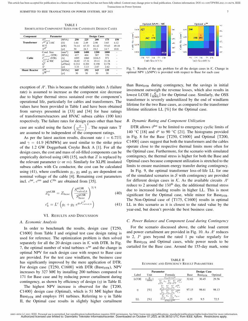
In order to benchmark the results, design case T250,C1600 from Table I and original test case design rating isused for reference. The optimization problem is then solvedseparately for all the 20 design cases in K with DTR. In Fig.7, the optimal number of wind turbines ntur and the change inoptimal NPV for each design case with respect to Base caseare provided. For the test case windfarm, the business casehas significantly improved by the mere application of DTR.For design case T250, C1600 with DTR (BaseDTR), NPVincreases by 327 Me by installing 200 turbines compared to171 for Base case and by reducing power curtailment duringcontingency, as shown by efficiency of design (η) in Table II.

The highest NPV increase is observed for the T200,C1400 design case (Optimal), which is 51 Me higher thanBaseDTR and employs 191 turbines. Referring to η in TableII, the Optimal case results in slightly higher curtailment

Fig. 7. Results of the opt. problem for all the design cases in K. Change inoptimal NPV (∆NPV) is provided with respect to Base for each case

than BaseDTR during contingency, but the savings in initialinvestment outweigh the revenue losses, which also results inlowest LCOE [ e

MWh ] for the Optimal case. Similarly, the OSStransformer is severely underutilized by the end of windfarmlifetime for the two Base cases, as compared to the transformerlifetime utilization LL [%] for the Optimal case.

B. Dynamic Rating and Component Utilization

DTR allows ϑhst to be limited to emergency cyclic limits of140 C [18] and ϑc to 90 C [21]. The histograms providedin Fig. 8 for the Base T250, C1600 and Optimal T200,C1400 cases suggest that both the transformers and the cablesoperate close to the respective thermal limits more often forthe Optimal case. Furthermore, for the scenario with simulatedcontingency, the thermal stress is higher for both the Base andOptimal cases because component utilization is stretched to thelimits to ensure maximum energy transfer during contingency.

In Fig. 9, the optimal transformer loss-of-life LL for oneof the simulated scenarios in S with contingency are providedfor different design cases in K. As the available circuits Ac

reduce to 2 around the 150th day, the additional thermal stressdue to increased loading results in higher LL. This is mostsignificant for the Optimal case, while minor for BaseDTR.The Non-Optimal case of T175, C1600 results in optimalLL in this scenario as it is closest to the rated value by theyear-end, but doesn’t provide the best business case.

C. Power Balance and Component Load during Contingency

For the scenario discussed above, the cable load currentand power curtailment are provided in Fig. 10. As Ac reducesto 2, Ic goes beyond the rated 1 pu value regularly forthe BaseDTR and Optimal cases, while power needs to becurtailed for the Base case. Around the 155-day mark, some

TABLE IIECONOMIC AND EFFICIENCY RESULT PARAMETERS

Parameter Design CaseLabel Unit Formula Base BaseDTR OptimalLCOE [ e

MWh ] Co(1+i)y∑y∈Y

πs∑

s∈S

∑t∈T

Pinjt,s

32.62 30.45 29.56

η [%]

∑y∈Y

∑s∈S

∑t∈T

Pinjt,s∑

y∈Y

∑s∈S

∑t∈T

Pgent,s

97.15 98.61 98.13

LL [%]

∑y∈Y

πs∑

s∈Sλy,s

8760 ΠWF 4.25 9.5 72.5





Fig. 8. Histograms for transformer HST ϑhst and cable conductor temperatureϑc (incl. seabed temp. ϑsea) for two scenarios in S (with & withoutcontingency) for BaseT250, C1600 & Opt.T200, C1400 cases

Fig. 9. System availability Ac and transformer loss-of-life LL (days) forscenario with contingency.

curtailment is also needed for the Optimal and BaseDTR casesbecause ϑc and ϑhst reach their respective limits, as shown inFig. 11. By comparing the Base and BaseDTR results directlyfrom Fig. 10, it conceivable that under static rating, higherwind energy curtailment would be needed under unfavorableambient conditions and when transmission system has inherentthermal bottlenecks

D. Impact of Approximation and Sensitivity Analysis

There are two important simplifications performed in theproposed methodology: cable thermal estimation and lineariza-tion of critical functions including component losses andtransformer ageing. Therefore it is important to substantiatethe impact of these approximations on the procedure’s perfor-mance.

As mentioned earlier, the simplified cable TEE model ismore conservative than the complex model of [21]. This isfurther confirmed in Fig. 12(a), where the time series forerror between the conductor temperature calculations of thetwo models are provided for the three test cases under consid-eration. As part of the post-process, the output load profiles ofthe optimization problem are passed through the complex TEEmodel to obtain the more accurate conductor temperature time-series ϑc

act. The period and scenario presented in the figure arespecifically chosen to represent the largest error found in thesimulation. It can be seen that ∆ϑc = ϑc

act − ϑcsup is mostly

positive. The difference is found to be in the range of -2 and7 C for all the simulated scenarios. Furthermore, in order to

Fig. 10. Scenario with contingency. Top: system availability Ac and loadcurrent Ic. Bottom: curtailed power Pcut [pu] with Pgen as base.

Fig. 11. Transformer HST ϑhst and cable conductor temperature ϑc (incl.seabed temp. ϑsea) in contingency scenario for BaseT250, C1600 &Opt.T200, C1400 cases. Respective thermal limits are also mentioned.

demonstrate the impact of this error on the business case, thedifference in wind power curtailment is provided in Fig. 12(b),where ∆P cut = P cut

act − P cutsup. The simplified model results in

higher curtailment when cable is the major thermal bottleneckin the system. Since the power transmission is not thermallygoverned in Base case, no change in power curtailment is seen.However, minor decrease in P cut is seen for the BaseDTR casecompared to the optimal case.

The linearization function proposed for losses and ageingapproximation are found to have minor influence on theconcerned parameters, as shown in Fig. 13. The temporal errorin cable losses ∆Wc, transformer losses ∆Wtrf and transformerageing ∆LLtrf is shown to be minimal, where each of these

Fig. 12. Impact of simplified cable thermal estimation on model’s perfor-mance for the three design cases. a: error in conductor temperature, b: errorin curtailed power





TABLE IIINORMALIZED MEAN SQUARE ERROR (%) FOR THE RELEVANT

PARAMETERS DUE TO THE PROPOSED APPROXIMATION METHODS.

Approx-imation Type

NMSE(X) [%] Design CaseX Definition Base BaseDTR Opt.

LossesLineraization

W tot Error in totalsystem losses 0.93 0.99 1.01

NPV Error in NPV(business case) 0.081 0.111 0.075

Trafo LLLinearization LLtrf Error in trafo

Life Loss 1.58 1.92 1.78

Cable TEESimplification

ϑc Error in cond.temp. 1.81 2.02 2.01

P cutc

Error in curt.power 0 0.12 0.18

is the difference between actual (non-linear function) andsupposed (linearized version). In order to quantify the overallimpact of these approximations on the parameter estimationand business case, Normalized Mean Square Error NMSEfrom (42) is used. NMSE allows normalization of error withthe standard deviation and is used extensively for statisticalbenchmarking [31]. NMSE of 100 would mean the predictivemodel is only as good as the mean model, while 0 would meana perfect match. The results are summarized in Table III for thechosen test cases. It can be seen that despite the approximation,the estimated values are very close to the actual ones and theapproximation method is found to have minor influence on theoverall system performance. Transformer lifetime utilization inparticular is on the high end, but the difference of upto 2%over 30-year lifetime is minor when compared to the valuesof Table II.

Fig. 13. Impact of piece-wise linearization on model’s performance for thethree design cases. a: error in cable losses, b: error in transformer losses, c:error in transformer lifetime utilization.

NMSE(X) = 100

[∑s∈S

∑t∈T

(Xactt,s − Xsup

t,s

)2∑s∈S

∑t∈T

(Xactt,s − Xµt,s

)2]

(42)

E. Out-of-Sample Validation

The results presented so far are obtained for the originallysimulated scenarios of the optimization framework. In order to

evaluate the general performance of the proposed methodologyand to remove any unwanted bias from the solutions, out-of-sample validation is used [31]. This is performed by simulatingthe optimization problem over a new set of scenarios s′ in S ′for the selected design cases. The objective function, primarydecision variables and the main constraints of the originalproblem remain intact for this step, with the exception of thewindfarm size (ntur) in constraint (21). By fixing the parameterntur to the optimal value identified by the original optimizationproblem for each of the design case, sensitivity of the solutionsto the scenario dataset is successfully analysed.

For the given test case, five simulations are run with 30unique scenarios (ns

′) each. The uncertainty in the simulated

values of the main decision variable (NPV) is calculated usingNormalized Root Mean Square Deviation (NRMSD) [%], asshown in (43). The change in optimal NPV of the originalsimulation (from Fig. 7) is represented by ∆NPVS , while∆NPVs′ is the change in optimal NPV for each of the uniquescenarios in S ′.

NRMSDk =

1ns′

√∑s′∈S′ (∆NPVs′ −∆NPVS)

2

∆NPVS(43)

The results of out-of-sample validation are provided in TableIV along with the 95% confidence interval, where 0% meansthat the results from original scenario simulation and the out-of-sample simulation are perfectly aligned. Furthermore, the95% confidence interval values for NRMSD are also providedin the table. It can be seen that there are no major outliersin these calculations and even after running five differentsimulations, the results from new scenario sets are alignedwith the originally trained scenario set for four out of fivesimulations. It is important to mention that 4% has beenchosen to be the critical breakeven point because ∆NPV inFig. 7 between the relevant design cases is around 4.5 %.Hence, as long as the NRMSD is below 4%, the algorithm iscertain to return the same design case as optimal.

TABLE IVNRMSD CALCULATIONS FOR OUT-OF-SAMPLE VALIDATION

Sim.No.

BaseDTRT250, C1600

OptimalT200, C1400

Non-OptimalT225, C1400

NRMSD NRMSD NRMSD95% Conf. Int. 95% Conf. Int. 95% Conf. Int.

1 2.32 % 2.15 % 2.01 %2.30% 2.33% 2.14% 2.16% 1.99% 2.03%

2 1.94 % 1.87 % 1.88 %1.90% 1.97% 1.83% 1.89% 1.85% 1.91%

3 3.93 % 4.12 % 3.96 %3.85% 4.00% 4.04% 4.19% 3.91% 4.01%

4 4.20 % 3.93 % 3.74 %4.16% 4.24% 3.90% 3.96% 3.72% 3.76%

5 2.95 % 2.82 % 2.79 %2.91% 2.98% 2.80% 2.85% 2.77% 2.82%

VII. CONCLUSION

A comprehensive, Dynamic Thermal Rating (DTR) based,two-stage stochastic model has been put forward in this paper,which can be used as investment decision support for OWFdesign and HVAC-based transmission system optimization.





The two-stage problem resolves investment decision by defin-ing optimal windfarm size in the first stage and DTR-basedcomponent ratings with the inclusion of scenarios of stochas-ticity in wind generation and transmission system reliabilityin the second stage. The proposed lumped TEE model for HVsubsea cables is proven to be fit for linear optimization withacceptable accuracy. The application of the proposed meth-odology on an actual test case windfarm indicates that mereapplication of DTR during operation increases the businesscase significantly which is further improved by DTR-baseddesign. This engineering model can be used as a decision toolfor design optimization and planning of large OWFs and theirtransmission systems, as it is generic enough to be expandedto different topologies of HVAC-based OWF transmission.

REFERENCES

[1] C. Walsh and D. Fraile, “Offshore wind in europe - key trends andstatistics 2019 (wind europe),” https://windeurope.org/, Feb 2020.

[2] P. Hou, J. Zhu, G. Yang, and Z. Chen, “A review of offshore windfarm layout optimization & electrical system design methods,” Jour. ofModern Power Systems & Clean Energy, vol. 7, pp. 975–986, 2019.

[3] H. Park and R. Baldick, “Transmission planning under uncertainties ofwind and load: Sequential approximation approach,” IEEE Trans. onPower Systems, vol. 28, no. 3, pp. 2395–2402, Aug 2013.

[4] J. Perez-Rua, M. Stolpe, K. Das, and N. A. Cutululis, “Global optimiza-tion of offshore wind farm collection systems,” IEEE Trans. on PowerSystems, vol. 35, no. 3, pp. 2256–2267, May 2020.

[5] M. Banzo and A. Ramos, “Stochastic optimization model for electricpower system planning of offshore wind farms,” IEEE Trans. on PowerSystems, vol. 26, no. 3, pp. 1338–1348, Aug 2011.

[6] S. Wei, L. Zhang, Y. Xu, and F. Li, “Hierarchical optimization for thedouble-sided ring structure of the collector system planning of largeoffshore wind farms,” IEEE Trans. on Sustainable Energy, vol. 3, no. 8,pp. 1029–1039, Jul 2017.

[7] J. Gonzalez, M. Payan, and J. Santos, “A new and efficient method foroptimal design of large offshore wind power plants,” IEEE Trans. onPower Systems, vol. 28, no. 3, pp. 3075–3084, Aug 2013.

[8] H. Ergun, D. V. Hertem, and R. Belmans, “Transmission system topol-ogy optimization for large-scale offshore wind integration,” IEEE Trans.on Sustainable Energy, vol. 3, no. 4, pp. 908–917, Oct 2012.

[9] M. Sedighi, M. Moradzadeh, and M. Fahrioglu, “Simultaneous opti-mization of electrical interconnection configuration and cable sizing inoffshore wind farms,” Jour. of Modern Power Systems & Clean Energy,vol. 6, pp. 749–762, 2018.

[10] H. Park, R. Baldick, and D. Morton, “A stochastic transmission planningmodel with dependent load and wind forecasts,” IEEE Trans. on PowerSystems, vol. 30, no. 6, pp. 3003–3011, Jan 2015.

[11] A. Cerveira, A. Sousa, and J. Baptista, “Optimal cable design of windfarms: The infrastructure and losses cost minimization case,” IEEETrans. on Power Systems, vol. 31, no. 6, pp. 4319–4329, Nov 2016.

[12] J. Perez-Rua, K. Das, and N. A. Cutululis, “Optimum sizing of offshorewind farm export cables,” International Journal of Electrical Power &Energy Systems, vol. 113, pp. 982–990, Dec 2019.

[13] S. Catmull, R. D. Chippendale, and J. A. Pilgrim, “Cyclic load profilesfor offshore wind farm cable rating,” IEEE Trans. on Power Delivery,vol. 31, no. 3, pp. 1242–1250, June 2016.

[14] M. A. H. Colin and J. A. Pilgrim, “Offshore cable optimization byprobabilistic thermal risk estimation,” in IEEE International Conferenceon Probabilistic Methods Applied to Power Systems, USA, 2018.

[15] S. H. Kazmi, T. Laneryd, and J. Holboll, “Cost optimized dynamic de-sign of offshore windfarm transformers with reliability and contingencyconsiderations,” Int. Journal of Electrical Power & Energy Systems, vol.Provisionally Accepted, 2020.

[16] N. Viafora, K. Morozovska, and S. H. Kazmi et al, “Day-ahead dispatchoptimization with dynamic thermal rating of transformers and overheadlines,” Electric Power Systems Research, vol. 171, pp. 194–208, 2019.

[17] J. Teh and I. Cotton, “Reliability impact of dynamic thermal ratingsystem in wind power integrated network,” IEEE Trans. on Reliability,vol. 65, no. 2, pp. 1081–1089, 2016.

[18] Guide for Loading Mineral-Oil-Immersed Transformers and Step-Voltage Regulators - Redline, IEEE C57.91-2011 Std., Mar 2011.

[19] Loading guide for oil-immersed power trafos, IEC 60076-7 Std., 2018.[20] N. Viafora, S. Kazmi, T. Olesen, T. Sørensen, and J. Holbøll, “Load dis-

patch optimization using dynamic rating and optimal lifetime utilizationof transformers,” in Proceedings of IEEE PES Powertech, Italy, 2019.

[21] Calculation of the Cyclic and Emergency Current Rating of Cables. Part2: Cyclic Rating of Cables Greater Than 18/30 (36) kV and EmergencyRatings for Cables of all Voltages, IEC60853-2 Std., AD:2008.

[22] R. Olsen, G. Anders, J. Holboll, and U. S. Gudmundsdottir, “Modellingof dynamic transmission cable temperature considering soil-specificheat, thermal resistivity and precipitation,” IEEE Transactions on PowerDelivery, vol. 28, no. 3, pp. 1909–1917, July 2013.

[23] D. Chatzipetros and J. A. Pilgrim, “Review of the accuracy of singlecore equivalent thermal model for offshore wind farm cables,” IEEETrans. on Power Delivery, vol. 33, no. 4, pp. 1913–1921, August 2018.

[24] S. Kazmi, T. Olesen, and J. Holbøll, “Machine learning based temper-ature forecast for offshore windfarm export cables,” in CIGRE SC B1(Insulated Cables For Future Power Systems). Paris: CIGRE, 2020.

[25] A. Madariaga, J. Martın, and O. A. Lara, “Effective assessment ofelectric power losses in three-core xlpe cables,” IEEE Trans. on PowerSystems, vol. 28, no. 4, pp. 4488–4495, Nov 2013.

[26] H. Brakelmann, “Loss determination for long three-phase high-voltagesubmarine cables,” Eur. Trans. Elect. Power, vol. 13, no. 3, pp. 193–197,Nov 2003.

[27] O. Gouda, G. F. Osman, W. A. Salem, and S. H. Arafa, “Cyclic loadingof underground cables including the variations of backfill soil thermalresistivity and specific heat with temperature variation,” IEEE Trans. onPower Delivery, vol. 33, no. 6, pp. 1242–1250, Jan 2019.

[28] R. Billinton and R. N. Allan, Reliability Evaluation of EngineeringSystems: Concepts and Techniques. New York, USA: Plenum, 1992.

[29] Y.-K. Wu, P. E. Su, Y.-S. Su, and W. S. Tan, “Economics and reliability-based design for an offshore wind farm,” IEEE Trans. on IndustryApplications, vol. 53, no. 6, pp. 5139–5149, Jan 2018.

[30] P. Chen, T. Pedersen, and B. Bak-jensen, “Arima-based time series modelof stochastic wind power generation,” IEEE Trans. on Power Systems,vol. 25, pp. 667–676, 2010.

[31] H. Madsen, Time Series Analysis. New York, USA: Chapman & HallCRC, 2008.

[32] J. Jurgensen, L. Nordstrom, and P. Hilber, “Estimation of individualfailure rates for power system components based on risk functions,”IEEE Trans. on Power Delivery, vol. 34, no. 4, pp. 1599–1607, 2019.

[33] W. G. A2.37, “Transformer reliability survey,” CIGRE TechnicalBrochure, p. 122, Aug 2015.

[34] J. Warnock, D. McMillan, J. Pilgrim, and S. Shenton, “Failure rates ofoffshore wind transmission systems,” Energies, vol. 12, no. 14, p. 2682,June 2019.

[35] BVG, “Guide to an offshore wind farm (updated),” https://ore.catapult.org.uk/app/uploads/2019/04/BVGA-5238-Guide-r2.pdf, April 2019.

Syed Hamza H. Kazmi received his B.E. (withdistinction) in Electrical Engineering from NEDUniversity, Karachi, Pakistan in 2014 and M.Sc inElectrical Energy Engineering (with Cum Laude)from the Delft University of Technology, Delft,The Netherlands in 2017. He finished his IndustrialPh.D. at Ørsted and at the Department of ElectricalEngineering in the Technical University of Den-mark. Currently, he is working as a Project Managerin Technology Development for Ørsted OffshoreWind Power. His main fields of interest are multi-

functional energy systems, electrical systems in connection with offshore windenergy and evolution of future offshore grids.

N. Viafora (S’18) received the B.Sc in EnergyEngineering and the M.Sc in Electrical Energy En-gineering from the Universita degli Studi di Padova,Padova, Italy, in 2013 and 2016, respectively. Hewas awarded the Ph.D. degree by the Department ofElectrical Engineering at the Technical Universityof Denmark in 2020. His research interests includeoptimization and decision-making in power systems,uncertainty modelling and dynamic line ratings.In 2020 he joined the Nordic Regional SecurityCoordinator in Copenhagen, Denmark, focusing on

coordinated security analysis.


https://windeurope.org/

https://ore.catapult.org.uk/app/uploads/2019/04/BVGA-5238-Guide-r2.pdf

https://ore.catapult.org.uk/app/uploads/2019/04/BVGA-5238-Guide-r2.pdf




Troels S. Sørensen received the M.Sc. and Ph.D.degrees in electrical engineering from the TechnicalUniversity of Denmark, Kgs. Lyngby, Denmark, in1990, and 1995, respectively. Currently, he is Sr.Director and Chief Specialist for Electrical Systemswith Ørsted Offshore Wind Power. He is workingwithin the fields of electrical power generation,transmission, and distribution. Presently his mainfields of work are electrical systems in connectionwith offshore wind energy and future offshore grids.

Thomas H. Olesen Thomas H. Olesen works asLead HV/MV Engineer in the Transformers andHV Components Engineering Department in ØrstedOffshore Wind Power, Denmark. He graduated witha B.Sc. in Electrical Engineering from the Universityof South Denmark in 2006. He has a comprehensiveexperience in development, commissioning, refur-bishment and lifetime extension of Offshore WindPower Plants (OWPPs), while he is currently work-ing on Hydrogen production and P2X generation inOWPPs. His research interests include oil-filled HV

components design and installation in offshore and onshore substations, andhe is a member of a number of working groups in CIGRE and IEC for shuntreactors and large power transformers.

Bikash C. Pal (M’00-SM’02-F’13) received B.E.E.(with honors) degree from Jadavpur University, Cal-cutta, India, M.E. degree from the Indian Instituteof Science, Bangalore, India, and Ph.D. degree fromImperial College London, London, U.K., in 1990,1992, and 1999, respectively, all in electrical engi-neering. Currently, he is a Professor in the Depart-ment of Electrical and Electronic Engineering, Impe-rial College London. . His current research interestsinclude renewable energy modelling and control,state estimation, and power system dynamics. He is

Vice President Publications, IEEE Power & Energy Society. He was Editor-in-Chief of IEEE Transactions on Sustainable Energy (2012-2017) and Editor-in-Chief of IET Generation , Transmission and Distribution (2005-2012) andis a Fellow of IEEE for his contribution to power system stability and control.

Joachim Holbøll is professor of High Voltage Engi-neering at Technical University of Denmark (DTU),Department of Electrical Engineering. He receivedhis Ph.D. degree from DTU in 1992. After someearly years with studies within high voltage insu-lation and electrical phenomena, J. Holbøll’s mainfield of research is now high voltage components,their properties and condition in close relation toadvanced modelling. Past years focus has been onhigh voltage transformers, cables and, in general,components’ performance under AC, DC and tran-

sients. The work is now concentrated on wind energy components and highvoltage research with respect to the future power grid. He is a Senior Memberof IEEE and member of Cigre National Committee of Denmark.


Offshore Windfarm Design Optimization using Dynamic Rating ...

Documents

Transcript of Offshore Windfarm Design Optimization using Dynamic Rating ...