MENTATiON PAGE j,•form Approved

'C"4 NIt I'C 'C'--AD- A267 488... ' .Q 1 .... I .. ........ f

ElO111111 It 11111 DATE REPORT TYPE AND DATES COVERED

__1993 THW/DISSERTATION4. T1,LE AND SUBTITLE 5. FUNDING NUMBERS

Full and Partial Multicommodity Cuts D T IC6. AUTHOR(S)

AG6 19

Roger Chapman Burk S7. PiRFORMING ORGANIZATION NAME(S) AND ADDRESS(ES) 18. PERFORM,.ING ORGA;:ZATION

REPORT NUMBER

AFIT Student Attending: Univ of North Carolina AFIT/CI/CIA 933D

;9. SP.t';,(JONG. MONITORING AGENCY NAME(S) AND ADDRESS(ES) 10. SPONSORR. G, MONITOý'ING

DEPARTMENT OF THE AIR FORCE AGENCY REPORT NUMBER

AFIT/CI2950 P STREETWRIGHT-PATTERSON AFB OH 45433-7765

i 12a. WTRi0,1TIO' A\,;'I'AE'!.:.ITY STATEMENT 120. DISTRWBUTION CCUE

Approved for Public Release IAW 190-1Distribution UnlimitedMICHAEL M. BRICKER, SMSgt, USAFChief Administration

13•,... AIISTRA;,. '', " " • ,rn, 2,?n' worw:)

9' 93-18086

7 11, SUBJ..T E[RMS 15 NUMBER OF PAGES

15316. PRICE CODE

S17. •-%URITY CLA'2IFiQATION 18 SECUEfY CLASSIi(CAT!ON IS. SECURITY CLASSIFICATION 20 LIMITATION CF ABSTRACTor REPOIMT C FC THIS PAGE OF ABSTRACT

I 1 _

p, " .. 1,.LIS ar •• : ,-" '• lq , •

:u -m | I

FULL AND PARTIAL MULTICOMMODITY CUTS

by

Roger Chapman Burk

A dissertation submitted to the faculty of

The University of North Carolina at Chapel Hill

in partial fulfillment of the requirements for the degree of

Doctor of Philosophy in the Department of Operations Research

Chapel Hill, 1993

Approved by:

I TIC Q"T t'JT" ' TT79Pfr.('7T D 3 61 ...

Adv~sor: J. Scott Provan

"NI'S CRAMI/

U',,.',.O' 2' ed c Reader: Thomas H. Brylawski? ": t- C

U'irabulson I Reader: Mark E. Hartmann

Av~IldeIity ColIes

Dest Sueceal Reader: David S. Rubin

'\ Jo W

Readelr: Jon W. Tolle

i m |K)

@1993Roger Chapman Burk

ALL RIGHTS RESERVED

•- • mI IiI

FULL AND PARTIAL MULTICOMMODITY CUTS

Roger Chapman Burk

(under the direction of Dr. J. Scott Provan)

ABSTRACT

The problems of finding multicommodity cuts and partial multicommodity cuts in

graphs are investigated. A multicommodity flow graph is a graph with k vertex pairs

identified as the terminals (source and sink) for k commodities. A (full) multicom-

modity cut is a set of elements (edges or vertices) whose removal from such a graph

cuts all source-to-sink paths for all commodities. A partial multicommodity cut is

defined as a set of elements whose removal prevents more than a given number r of

commodities from being connected by disjoint paths. For the full multicommodity

cut problem, polynomial algorithms are found for any fixed k in a T-planar graph

(one with all terminals on the boundary) and for k = 3 in a general planar graph. The

T-planar problem is shown to be NP-complete for varying k unless the terminals are

in non-crossing order; a polynomial algorithm is developed for that case. For partial

multicommodity cuts, polynomial algorithms are developed for r = k - 1, r = k - 2,

and r = I in T-planar non-crossing graphs. In the special case in which there is

a common source for every commodity, the partial multicommodity cut problem is

shown to be polynomial as long as r or k - r is bounded, even in general graphs.

111i.

TABLE OF CONTENTS

LIST OF FIGURES ................................ vi

LIST OF ABBREVIATIONS ........................... viii

1 INTRODUCTION .............................. 1

2 NOTATION AND DEFINITIONS ..................... 7

2.1 Set Theory .. .. .. .............. .... .. .... 7

2.2 Graph Theory ............................. 8

2.3 Multiterminal and Multicommodity Flow Graphs ............ 11

2.4 Complexity and Intractability .................... 14

3 SURVEY OF RELATED RESEARCH ................... 16

3.1 Multicommodity Flows ........................ 16

3.2 Multiterminal Cuts .......................... 18

3.3 Multicommodity Cuts ........................ 19

3.4 Disjoint Paths ............................. 21

4 GENERAL RESULTS ............................ 32

4.1 Full Multicommodity Cuts and Multiterminal Cuts ........... 32

4.2 Partial Multicommodity Cuts .......................... 36

4.3 Two Propositions on Intractability ...................... 37

5 FULL MULTICOMMODITY CUTS IN PLANAR GRAPHS ....... .. 39

5.1 The Modified Dual gD' and the Ue-PB MTC Problem ...... .. 40

5.2 The Ue-PBk FMCC Problem .......................... 43

5.3 The Non-T-planar Case with k = 3 ...................... 55

5.4 The Intractability of T-Planar Cuts when k Varies ............ 61

5.5 A Case that is Polynomial in k: Ue-P*BN ................. 70

iv

6 PARTIAL MULTICOMMODITY CUTS IN T-PLANAR GRAPHS ... 77

6.1 Disjoint Paths in Non-crossing T-Planar Graphs ............ 78

6.2 The Caseof r=- k- .1 ........................ 82

6.3 The Case of r =- k - 2 ........................ 85

6.4 The Case of r = 1 ........................... 89

7 THE EXTENSION TO VERTEX-CUTS .................. 102

7.1 The Face-dual gF and the Multiterminal Vertex-cut Problem. .. 103

7.2 The T-Planar Multicommodity Vertex-cut Problem with k Fixed 111

7.3 The Intractability of Vertex-cuts when k Varies ............. 114

7.4 A Polynomial Case: T-Planar and Non-crossing ............. 116

7.5 Partial Multicommodity Vertex-cuts ...................... 117

8 THE SINGLE-SOURCE PROBLEM .......................... 120

8.1 Arc-cuts, Arc-disjoint paths, r = 1 (DeE) .................. 121

8.2 Generalizing DeE to 1 < r < k .......................... 124

8.3 Generalizing to Cases UeE, DvV, and UvV ................ 129

8.4 The Cross-case DeV ....... ......................... 132

8.5 The Cross-case DyE ....... ......................... 137

8.6 Undirected Nearly T-Planar Graphs (UeEP) ................ 140

9 CONCLUSIONS AND FUTURE WORK ....................... 147

REFERENCES ........................................... 150

V

LIST OF FIGURES

1 Forbidden Configurations in W for Sufficiency of GCC in DJP U-EEu* 26

2 Extended GCC for D-VPB Problem (Example) ................... 30

3 The Optimal FMCC Is Not a Supreme Cut ...... ................ 34

4 Minimum Supreme Cut Leaving Two Components in 7 .............. 34

5 A Graph with at Least k + 1 Components in 1Z ................... 36

6 Construction of GD .. ................................................... 41

7 Proof of Proposition 5 ........ ............................ 42

8 Example of GDm for an MCF Graph ....... .................... 45

9 The T and S Functions (Example) ...... ..................... 49

10 T and S Functions in an Optimal FMCC (Example) ............... 50

11 The C, B, and D Functions (Examples) ...... .................. 52

12 Configurations for Ue-P3 FMCCs with Four Components in 1 ...... ... 57

13 Example of a Manacle Cut ................................. 58

14 Manacle Cut Not Using Shortest a-b Path ...................... 58

15 Vertex Gadget for Vertex vi . . . . . .. . . . . . . . . . . . . . . . . . . .. . . . . . 63

16 Edge Gadget for e, = (ve,vf) ............ ........................ ... 63

17 Vertex-associated Arms in Star ....... ....................... 68

18 Edge-associated Arms in Star ....... ........................ 68

19 The S Function in Ue-P*BN Case (Example) ................. 72

20 A Non-optimal Configuration in the Non-nested Case ............... 74

21 Proof of Lemma 5 ........ .............................. 79

22 Proof of Lemma 6 ........ .............................. 87

23 A U--P*BN One-disjoint-path Graph ...... ................... 91

vi

24 Three Non-disjoint Paths in RJT ........ ...................... 93

25 Trifid Cut as Part of a PMCC ............................... 95

26 J+3' Corresponding to a Trifid Cut J .......................... 96

27 Trifid Cut as Optimal FMCC in 9 - {e,f,g}. .................... 98

28 The Face-dual gF (Example) ....... ........................ 104

29 The Common Face of ci and ci+, . . .. . .. . . .. . . . . . . . . . . . . . .. . . . . . . . 106

30 Vertex Gadget for Vertex-cuts ............................... 115

31 Edge Gadget for Vertex-cuts ................................ 115

32 Proof of Lemma 11 ........ .............................. 122

33 Example of Side Condition Causing a Non-integral Simplex Solution.. 123

34 Construction of a Single-source PMCC ........................ 126

35 A PMCC Problem with k = 3, r - 2 ......................... 128

36 Single-source DeV Problem, k = 3, r = 2 ........................ 134

37 Mindeg-1 Nodes ........................................ 138

38 Finding a Node-cut Containing a Mindeg-1 Node ................. 138

39 Single-source DvE Problem, k = 3, r = 2 ........................ 139

40 FMCC Corresponding to Optimal PMCC in Sink-planar Graph ..... .. 141

41 Proof of Proposition 25 ................................... 143

42 The Recursive Formula for A([t.,tb],q) ....... ................... 144

vii

LIST OF ABBREVIATIONS

D-E a problem concerning arc-disjoint paths in a directed graph

D-V a problem concerning node-disjoint paths in a directed graph

D-V2 a problem concerning node-disjoint paths in a directed graph havingtwo commodities

D-VPB a problem concerning node-disjoint paths in a planar directed graphhaving all terminals on the boundary

De- a problem concerning removing arcs from a directed graph

DeE a problem concerning removing arcs from a directed graph and leavingarc-disjoint paths

DeV a problem concerning removing arcs from a directed graph and leavingnode-disjoint paths

DJP the disjoint paths problem (p. 21)

DyE a problem concerning removing nodes from a directed graph and leavingarc-disjoint paths

DvV a problem concerning removing nodes from a directed graph and ]eavingnode-disjoint paths

FMCC full multicommodity cut (problem or set of graph elements; p. 1)

GCC general cut condition (p. 23)

IC intersection criterion (p. 25)

IMCF integer multicommodity flow problem (p. 23)

MCC multicommodity cut (problem or set of graph elements; p. 1)

MCF multicommodity flow problem (p. 16)

MTC multiterminal cut (problem or set of graph elements; p. 18)

viii

PMCC partial multicommodity cut (problem or set of graph elements; p. 1)

U- -P*BN a problem concerning a planar undirected graph having all terminalson the boundary in non-crossing order

U- -P*Eu* a problem concerning an undirected graph that is planar and Eule-rian when augmented with the demand edges

U--PBEu* a problem concerning a planar undirected graph that has all termi-nals on the boundary and that is Eulerian when augmented with thedemand edges

U-E a problem concerning edge-disjoint paths in an undirected graph

U-E2 a problem concerning edge-diLjoint paths in an undirected graphhaving two commodities

U-EEu* a problem concerning edge-disjoint paths in an undirected graphthat is Eulerian when augmented with the demand edges

U-EP a problem concerning edge-disjoint paths in a planar undirectedgraph

U-EP* a problem concerning edge-disjoint paths in an undirected graphthat is planar when augmented with the demand edges

U-EP*BN a problem concerning edge-disjoint paths in a planar undirectedgraph having all terminals on the boundary in non-crossing order

U-EP*Eu* a problem concerning edge-disjoint paths in an undirected graphthat is planar and Eulerian when augmented with the demand edges

U-EPB a problem concerning edge-disjoint paths in a planar undirectedgraph having all terminals on the boundary

U-EPBEu* a problem concerning edge-disjoint paths in a planar undirectedgraph that has all terminals on the boundary and that is Eulerianwhen augmented with the demand edges

U-EPEu* a problem concerning edge-disjoint paths in a planar undirectedgraph that is Eulerian when augmented with the demand edges

ix

U-V a problem concerning vertex-disjoint paths in an undirected graph

U-V2 a problem concerning vertex-disjoint paths in an undirected graphha', ng two commodities

U-VP a problem concerning vertex-disjoint paths in a planar undirectedgraph

U-VPB a problem concerning vertex-disjoint paths in a planar undirectedgraph having all terminals on the boundary

U-VPk a problem concerning vertex-disjoint paths in a planar undirectedgraph having k commodities

Ue-P a problem concerning edge-cuts in a planar undirected graph

Ue-PIBN a problem concerning edge-cuts in a planar undirected graph havingall terminals on the boundary in non-crossing order

Ue-P3 a problem concerning edge-cuts in a planar undirected graph havingthree commodities

Ue-PB3 a problem concerning edge-cuts in a planar undirected graph havingall terminals on the boundary

Ue-PBk a problem concerning edge-cuts in a planar undirected graph that hasall terminals on the boundary and has k commodities

Ue-Pk a problem concerning edge-cuts in a planar undirected graph havingk commodities

UeE a problem concerning removing edges from an undirected graph andleaving edge-disjoint paths

UeEP*BN a problem concerning removing edges from a planar undirected graphthat has all terminals on the boundary in non-crossing order andleaving edge-disjoint paths

UeV a problem concerning removing edges from an undirected graph andleaving vertex-disjoint paths

lJv-PB a problem concerning vertex-cuts in a planar undirected graph havingall terminals on the boundary

x

UvE a problem concerning removing vertices from an undirected graph andleaving edge-disjoint paths

UvV a problem concerning removing vertices from an undirected graph andleaving vertex-disjoint paths

UvVPB a problem concerning removing -,ertices from a planar undirected graphhaving all terminals on the boundary and leaving vertex-disjoint paths

VLSI very large scale integrzted (circuit)

xi

1 INTRODUCTION

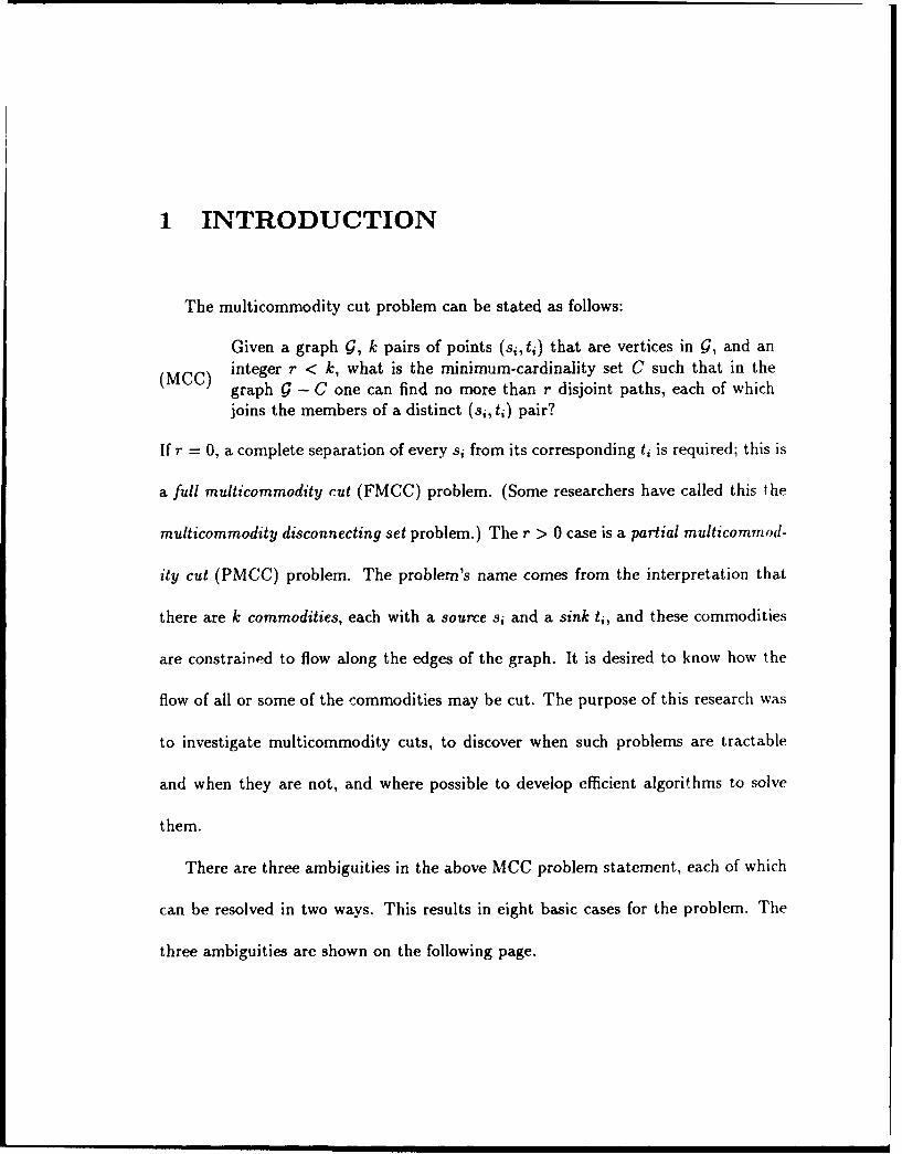
The multicommodity cut problem can be stated as follows:

Given a graph g, k pairs of points (si, ti) that are vertices in G, and an(MCC) integer r < k, what is the minimum-cardinality set C such that in the

graph Q - C one can find no more than r disjoint paths, each of which

joins the members of a distinct (si, ti) pair?

If r = 0, a complete separation of every si from its corresponding ti is required; this is

a full multicommodity cut (FMCC) problem. (Some researchers have called this the

multicommodity disconnecting set problem.) The r > 0 case is a partial multicommod-

ity cut (PMCC) problem. The problem's name comes from the interpretation that

there are k commodities, each with a source si and a sink ti, and these commodities

are constrained to flow along the edges of the graph. It is desired to know how the

flow of all or some of the commodities may be cut. The purpose of this research was

to investigate multicommodity cuts, to discover when such problems are tractable

and when they are not, and where possible to develop efficient algorithms to solve

them.

There are three ambiguities in the above MCC problem statement, each of which

can be resolved in two ways. This results in eight basic cases for the problem. The

three ambiguities are shown on the following page.

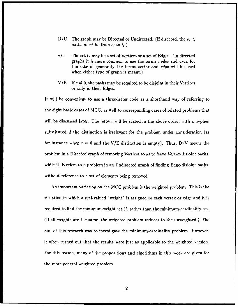
D/U The graph may be Directed or Undirected. (If directed, the si-tipaths must be from s. to t4.)

v/e The set C may be a set of Vertices or a set of Edges. (In directedgraphs it is more common to use the terms nodes and arcs; forthe sake of generality the terms vertex and edge will be usedwhen either type of graph is meant.)

V/E If r 0 0, the paths may be required to be disjoint in their Verticesor only in their Edges.

It will be convenient to use a three-letter code as a shorthand way of referring to

the eight basic cases of MCC, as well to corresponding cases of related problems that

will be discussed later. The letter's will be stated in the above order, with a hyphen

substituted if the distinction is irrelevant for the problem under consideration (as

for instance when r = 0 and the V/E distinction is empty). Thus, DvV means the

problem in a Directed graph of removing Vertices so as to leave Vertex-disjoint paths.

while U-E refers to a problem in an Undirected graph of finding Edge-disjoint paths,

without reference to a set of elements being removed

An important variation on the MCC problem is the weighted problem. This is the

situation in which a real-valued "weight" is assigned to each vertex or edge and it is

required to find the minimum-weight set C, rather than the minimum-cardinality set.

(If all weights are the same, the weighted problem reduces to the unweighted.) The

aim of this research was to investigate the minimum-cardinality problem. However,

it often turned out that the results were just as applicable to the weighted version.

For this reason, many of the propositions and algorithms in this work are given for

the more general weighted problem.

2

The Motivation for the Research

One of the motivations for this line of research was technical interest in the in-

terplay between combinatorial methods and minimum-cut methods rooted in linear

programming. Another was the hope that results from graph theory could be used to

make efficient algorithms to solve practical problems. However, the original focus of

interest was on an application in biochemistry, in theoretical modeling of metabolic

systems. This is just one of many applications of multicommodity cuts. Besides

the original problem in biochemistry, the most obvious applications are in military

planning and in communication network analysis.

The biochemical application comes from Kohn and Lemieux [19911, who proposed

a method of modeling the interacting biochemical reactions within a cell as a flow

network in which every reaction is represented as a node. The crucial self-regulating

properties of such a metabolic system are found in the feedback paths, i.e. the paths

that connect the product of a., enzyme-catalyzed reaction to a reactant of the same

reaction. A key step in aialyzing the regulatory properties of the network is finding

the smallest possible set of reactions such that at least one reaction is on every

feedback path. This can be formulated as an FMCC problem. The si-t, pairs are the

product-reactant pairs in each enzymatic reaction, and the set of reactions covering

every feedback path is a cut-set.

Military applications were the motivation for some of the first research on MCCs

[Bellmore, Greenberg, and Jarvis, 1970]. The supply network for an army in the

field can be modeled appropriately as a multicommodity flow network. The multiple

3

commodities can arise because different units take their support from different points,

or because different types of supplies (e.g. ammunition, food, fuel) have different

origins and destinations. The opposing force will want to attack this supply network

in the most economical manner possible in order to stop the flow of all or some

supplies. This can be formulated as an MCC problem.

The third important application of MCCs is in the reliability analysis of com-

munications networks. In this case, the si-ti pairs represent parties that need to be

connected. The problem is to find the smallest set of communication nodes or links

whose failure will prevent a separate line being assigned either to each pair or to

more than a given number of pairs. This is perhaps the most obvious and important

application for partial multicommodity cuts.

Outline of the Work

This work is in nine chapters. The next chapter (Chapter 2) gives formal defini-

tions for the terms used, establishes the notation and standard symbols to be used.

and where appropriate mentions restrictions on the types of problems considered.

Chapter 3 surveys current research on multicommodity cuts and on three related

problems: multicommodity flows, multiterminal cuts, and disjoint paths. Chapter 4

gives a few basic results on multicommodity cuts in order to set the stage for the

following chapters.

Chapter 5 is the central chapter in this work. The subject is full multicommodity

edge-cuts in planar graphs. After an initial section on the corresponding multiterminal

cut problem, a polynomially bounded algorithm is developed for a fixed number

4

of commodities when all the sources and sinks (collectively terminals) are on the

boundary of the graph. If the terminals are not restricted to the boundary the problem

is more difficult, but a polynomial algorithm is developed for the three-commodity

case. If the number of commodities is not fixed then the planar multicommodity cut

problem is shown to be NP-complete, even if the graph is a rectangular grid with

the terminals on the boundary. A final section in Chapter 5 shows that the problem

is polynomial if the terminals are on the boundary in what is called "non-crossing

order" (see p. 13), and develops an algorithm for that case.

Chapter 6 extends the discussion of MCCs in such graphs to include partial mul-

ticommodity cuts. This chapter develops algorithms for the k-commodity PMCC

problem in planar graphs with terminals on the boundary in non-crossing order when

the parameter r (the number of disjoint si-ti paths allowed to remain) is equal to

k - 1, k - 2, and 1.

Chapter 7 extends some of the major results of chapters 5 and 6 to vertex-cuts.

The general problem of multicommodity vertex-cuts in planar graphs with terminals

on the boundary is shown to be NP-complete if the number of commodities k varies,

but polynomial algorithms are presented for fixed k and for varying k with non-

crossing terminals. The partial multicommodity vertex-cut problem is solved for

r =k - 1.

Chapter 8 considers the special case in which all commodities have their sources

(or equivalently, their sinks) at the same vertex. This restriction makes the problem

easier in many ways. Even in general graphs full multicommodity cuts become easy,

• • m m |5

and the partial multicommodity cut problem is shown to be polynomially bounded

as long as either r or k - r is bounded. These results hold in directed graphs as well

as in undirected, and they hold for both edge- and vertex-cuts. In addition, the cases

DeV and DyE, in which nodes are removed from a graph to limit arc-disjoint paths

or vice versa, are investigated. Finally, in the special case of an undirected planar

graph with all sinks on the boundary, an algorithm is developed that is polynomially

bounded for arbitrary k and r.

Chapter 9 concludes this work by summarizing the results and describing some

likely directions for future research on multicommodity cuts.

6

2 NOTATION AND DEFINITIONS

This chapter lists definitions for terms used throughout this work. As far as

possible these are the standard definitions used in the relevant field of research. It

also gives some notation and symbology that will be constant for the rest of the work.

The areas covered are set theory, graph theory, multiterminal and multicommodity

flow graphs, and algorithmic complexity.

2.1 Set Theory

The empty set is designated q. An i-partition of a set S is a collection of i subsetsi

Sj of S such that US, = S and SaSb = s for any a 5 b. A partition is anyj=1

i-partition. The cardinality or size of a set is the number of its members; a set is

larger or smaller than another according as its cardinality is larger or smaller. A

subset Sj is said to be minimal with regard to some property if no proper subset of

it has that same property. It is minimum with regard to a property if no smaller

set at all has that property; thus a minimum set is also minimal but not vice versa.

Maximal and maximum are defined similarly.

The members of a set may have positive real-valued numbers called weights as-

sociated with them. In this case the weight of a set is the sum of the weights of

its members. In this work zero and negative weights will not be considered, since

the interest is in minimum-weight sets and any zero- or negative-weight elements can

automatically be included in the solution. In the context of an algorithm, the term

infinite will be used loosely to describe a weight assigned to an element that is large

enough to ensure the element's selection or nonselection, as appropriate.

A multiset is a collection of elements like a set, but unlike a set some of its elements

may occur more than once.

2.2 Graph Theory

The notation and terminology for graphs is generally that of Wilson [1985]. A

few modifications have been made in this work work to emphasize certain parallels

between multicommodity edge-cuts and multicommodity vertex-cuts.

e Definitions referring to graphs in general

- A graph, denoted Q, is a pair (V, E), where V is a nonempty finite set

of elements called vertices and E is a finite multiset of elements called

edges, each of which is a pair of elements of V. Sometimes E will loosely

be called an edge set, even though it may have repeated elements. In

this work loops (elements of E of the form (v, v)) will be disregarded as

irrelevant to multicommodity cut problems.

- The elements of E can be denoted (u, v) or uv.

- A graph is directed or undirected according as the elements of E are ordered

or unordered pairs. A directed graph is also called a digraph. The vertices

and edges of a digraph are also called nodes and arcs. In this work graphs

are undirected unless otherwise stated.

- For e = (u, v) E E, u and v are called the endvertices of e. The edge e and

its endvertices are said to be on each other.

- Two edges are parallel if they have the same endvertices.

8

- The degree of v E V is the cardinality of {e E E : e = (v,u) ore e

(u, v)} (disregarding loops). The in-degree of a node v in a digraph is the

cardinality of {e E E : e = (u, v)} and its out-degree is the cardinality of

{e E: e = (vu)}.

- A graph is Eulerian if the degree of every node is even.

- A subgraph of g is a graph !9' = (V', E') such that V' C V and E' C E.

- For any F C E, the subgraph induced by F is the graph whose edge set is

F and vertex set is all the vertices on members of F.

- For any F C E, g - F is the graph (V, E - F).

- For any U C V, • - U is the graph whose vertex set is V - U and whose

edge set is all members of E that are not on a member of U.

- ForanyxEEorxEV, 9-x-g-{X}.

e Definitions concerning planar graphs

- Every graph can be represented (not uniquely) by a set of points corre-

sponding to its vertices and a set of lines or curves connecting the points

and representing its edges. A graph is planar if it has a representation that

is embedded in a plane and in which no two edge lines intersect except at

the vertex points. In this work a planar graph will be considered together

with a fixed representation in a plane; this combination is called a plane

graph.

- A grid is a plane graph whose representation is a subset of a rectangular

lattice.

- The edges of a planar graph g divide the plane into a number of regions.

exactly one of them infinite in extent. These are the faces of g.

- The boundary of a planar graph is the boundary of its infinite face.

- The geometric-dual gD . (VD, ED) of a planar graph Q has exactly one

vertex for every face in • and exactly one edge for every edge. An edge in

E D connects two vertices in VD if and only if the corresponding edge in E

is in the common boundary of their corresponding faces in Q.

* Terms having to do with paths and connectivity in graphs

- A path in a graph is a sequence of distinct edges of the form (vo, vi), (vI, v2 ),

... , (ve-1,vt) such that v. A vb if a 6 b, except that possibly v0 = vy. A

path in a digraph can be directed in the obvious way.

9

- A circuit is a path in which vo = Vt.

- A triangle is a circuit of three edges.

- A path is covered by the edges in it and by the endvertices of those edges.

- The union of two graphs 91 = (V1,E 1 ) and ! 2 = (V2, E 2) is the graph

(V U V2, E1 U E2).

- A graph is connected if it cannot be represented as the union of two graphswith disjoint vertex sets; otherwise it is disconnected. All graphs considered

in this work are connected unless stated otherwise.

- A component of a graph is a maximal connected subgraph. Thus a con-nected graph has exactly one component.

- A disconnecting set is any X C E or X C V such that g-X is disconnectedor empty. In this work a disconnecting set will be an edge set unless

otherwise stated.

- A graph is i-edge-connected if the size of its smallest disconnecting edge setis i or more. It is i-vertex-connected if the size of its smallest disconnectingvertex set is i or more.

* Definitions regarding edge- and vertex-cuts in graphs

- A minimal disconnecting set is a cut-set or a simple cut. It can also be

called an edge-cut or vertex-cut, as appropriate. A cut-set will be an edge-cut in this work unless otherwise stated.

- An i-way cut or i-cut is a minimal set X C E or X C V such that g - X

has exactly i components. Thus a two-way cut is a cut-set. When thecontext is clear, an i-way cut can also be called an cdge-cut or vertex-cut,as appropriate.

- A compound cut is an i-way cut with i > 2.

- For any U C V, [(U) denotes the set of edges with one endvertex in Uand the other in V - U. Thus 1(U) is a simple cut or can be partitioned

into simple cuts.

- Suppose in a digraph there is a directed path from node v to node u. Thena v-u directed cut is a minimal set of arcs or nodes X such that C - Xcontains no such path.

- An edge-cut of size 1 is also called a bridge.

- A vertex-cut of size 1 is also called an articulation vertex.

10

* Terminology concerning trees and forests

- A forest is a graph that contains no circuits.

- A tree is a connected forest.

- For any U C V, the Steiner tree on U is a connected subgraph of 9whose vertex set includes U and whose edge set has minimum cardinalityor minimum weight.

A flow problem can be defined on a directed or undirected graph by designating

one vertex as a source, one vertex as a sink, and assigning a capacity to each edge.

Among the well-known consequences of the work of Ford and Fulkerson (19561 are

efficient algorithms to find a maximum feasible flow in such a problem and a minimum

capacity edge-cut between the source and the sink; the value of a maximum flow and

the value of a minimum capacity cut are the same. By reformulating the problem

the minimum weighted vertex-cut can also be found. Also, if all the capacities are

integer-valued, then there exists a maximum-flow solution such that every flow along

every edge (and consequently the total flow) is integer-valued.

2.3 Multiterminal and Multicommodity Flow Graphs

The multicommodity cut problem has already been defined (p. 1). This section

gives the standard conventions and notation that will be used in discussing such

problems and the graphs in which they occur. Some definitions will also be given for

the closely-related class of multiterminal graphs.

A multiterminal graph is an undirected graph ! = (V, E) together with a set of

terminals T C V. The cardinality of T will always be represented by k, and T =

11

{tI, t2,..., tk)}. An instance of a multiterminal cut problem is given by a multiterminal

graph !, which is assumed to include a designation of T.

A multicommodity flow graph is a directed or undirected graph G = (V, E) together

with a set of terminals T = {Sl, tI, S2, t2 ,. . , Sk, tk} C V. The following terms will

have constant meaning in this work when discussing multicommodity flow graphs.

Q The connected graph (V,E) along which the commodities flow; alsocalled the supply graph; IVI = n and IEI = m.

R The graph with the same vertices as g and edges (si,t•), i = 1,...k;

also called the demand graph

" with the edges of Hi added; also called the augmented supply graph

k The number of commodities

T The set of vertices that are terminals; 2 < ITI < 2k, since some ofthe terminals may be co-located

r The allowed number of disjoint paths in a partial multicommoditycut problem

C A minimal solution to a full multicommodity cut problem, sometimescalled a full cut or full multicommodity cut (FMCC) when no ambi-guity results

J A minimal solution to a partial multicommodity cut problem, calledan interjacent set; also called a partial cut or partial multicommoditycut (PMCC) when no ambiguity results (a minimal interjacent setneed not be a cut-set or even a disconnecting set)

IZ The remaining graph g - C or g - J

The terminals sj and tj are mates of each other and are required to be distinct; they

constitute a terminal pair or pair of terminals. A solution will be said to separate a

commodity j if there is no sj-tj path in TZ. Two components of RZ will be said to

share a commodity j if one of them contains sj and the other ti. An instance of a

12

multicommodity cut problem is given by a multicommodity flow graph ' (which is

assumed to include T) and r.

In vertex-cut problems in multiterminal and multicommodity flow graphs, the

terminals themselves are always taken to be ineligible to be in the solution.

A multiterminal graph or multicommodity flow graph is T-planar if it is planar

and has a representation with all terminals on the boundary. In a T-planar graph,

two terminals are adjacent if there is a path from one to the other that runs around

the boundary of g and contains no other terminals. The members of a sequence

of terminals each of which is adjacent to the next is a set of consecutive terminals.

In a T-planar multicommodity flow graph, two commodities i and j are interleaved

or in interleaved order if their terminals occur in order si, sj, ti, tj either clockwise or

counterclockwise around the boundary of g'; otherwise they are in non-crossing order.

A graph is non-crossing if all the commodities in it are. The order of terminals in a

multiterminal graph is without significance.

A multicommodity cut problem is unwveighted if the solution of smallest cardinality

is sought. If the relevant elements have a weight defined on them and the minimum

weight solution is sought, then the problem is weighted. Thus an unweighted problem

is equivalent to a weighted one in which all weights are the same. All problems in

this work are unweighted unless otherwise stated.

The descriptive codes introduced in Chapter 1 (DvV, U-E, etc.) will be used as a

shorthand to designate particular cases of multicommodity cut and related problems.

In addition, it will be convenient to add letter codes to designate particular graph

13

configurations that are frequently studied:

P The graph g is planar

P* The graph g* is planar

Eu The graph g is Eulerian (all vertices of even degree)

Eu* The graph g* is Eulerian

B In a planar graph, all terminals are on the boundary

N In a planar graph with all terminals on the boundary, the ter-minals are in non-crossing order

2,3,... The number of pairs of terminals (parameter k) is 2, 3,

Thus, MCC UvVP*B2 would designate a multicommodity vertex-cut problem in an

undirected graph in which the remaining paths are to be vertex-disjoint, Q augmented

by all edges (si, ti) is planar, all terminals are on the boundary of one face of 9, and

there are two commodities. A general T-planar multicommodity cut problem is Ue-

PB and a non-crossing one is Ue--P*BN.

Unless otherwise stated, in this work a multicommodity cut problem will be a full

multicommodity edge-cut problem in an undirected graph (Ue-).

2.4 Complexity and Intractability

The reader is assumed to be generally familiar with the theory of intractability as

given (for instance) in Garey and Johnson [19791, from which the following definitions

are taken. A function f(x) is O(g(x)) if there is a constant c such that If(:) _<

clg(x)I for all sufficiently large non-negative values of x. An algorithm is said to

be polynomial time, polynomially bounded, or simply polynomial if the number of

14

operations it performs is O(p(y)), where y is an encoding of the algorithm's input

and p(y) is a polynomial in y. The algorithm and the work in it are also said to be

O(p(y)). A problem is said to be polynomial or polynomially bounded if it can be

solved with a polynomial algorithm. The term NP-complete describes a certain large

and well-studied class of decision problems, all of which can be reduced to the others

in polynomial time and for none of which is a polynomial algorithm known. (We refer

the reader to Garey and Johnson for a specific definition of this class.) A problem

is NP-hard if a polynomial algorithm for it would imply a polynomial solution to an

NP-complete problem.

A problem that will arise frequently in the algorithms in this work is that of finding

the shortest paths between all pairs of vertices in a planar g-aph. This problem is

known to be O(n'), where n is the number of vertices in the graph (Frederickson.

1987]. We will use O(a) to mean the complexity of the planar all-pairs shortest paths

problem.

15

3 SURVEY OF RELATED RESEARCH

Research that is relevant to the problem of full and partial multicommodity cuts

covers four topics: multicommodity flows, multiterminal cuts, (full) multicommodity

cuts themselves, and disjoint paths. A section of this chapter is devoted to each of

these. There is no published research specifically on partial multicommodity cuts,

but it is clearly related to the problem of finding disjoint si-ti paths in a multicom-

modity flow graph. This is a large problem in its own right. Separate subsections

in Section 3.4 will address the taxonomy of the many variations of the disjoint paths

problem, its computational complexity, its generalization in the integer multicom-

modity flow problem, and known results for some special cases.

3.1 Multicommodity Flows

A multicomnaodity flow problem concerns finding feasible flows in a given multi-

commodity flow graph g. In its decision-problem form it can be defined like this (all

values are assumed to be real and non-negative):

Given a multicommodity flow graph with maximum capacities defined on

(MCF) each edge, and with demands or total flows fi required between each pairof terminals (si, ti) for 1 < I < k, are there flows that are simultaneouslyfeasible and will satisfy every demand?

Other variations include the the construction problem (finding the feasible flows), the

maximum sum-of-flows problem, and the minimum cost problem (in which a cost per

unit flow for each edge is defined). MCF is a linear program in any of these forms,

and so in a sense it is a well-solved problem. Assad [19781 and Kennington (1978]

review and compare practical solution algorithms.

Other researchers have concentrated on what can be deduced about multicom-

modity flows by graph-theoretical methods. They have been particularly interested

in finding when the maximum feasible flow is equal to the smallest-capacity cut be-

tween all si and all ti vertices. This has long been known to be true for the case of one

commodity [Ford and Fulkerson, 1956]. In 1963 Hu [22] proved it for two commodities

in an undirected graph, and in 1980 Seymour [49] for up to six commodities if there

are no more than four distinct terminals. Other results have been limited to special

types of planar graphs. Okamura and Seymour [1981) showed that the maximum

flow equals minimum cut if g is T-planar, Seymour [1981b] if Q" is planar, Okamura

[1983] if ! is planar and has two faces such that each terminal pair is on one of them,

and Okamura [1983] again if ! is planar and every terminal pair is either on a given

face or shares one particular vertex on that face. Schrijver [1983] has summarized

results of this sort (except the last two). These specialized results have led to efficient

algorithms for finding feasible multicommodity flows on such graphs or for deciding if

such a feasible flow exists. These have been offered by Okamura and Seymour [1981b],

Hassin [1984], and Matsumoto, Nishizeki, and Saito [1985].

In these cases in which maximum flow equals minimum cut, the researchers also

showed that if the arc capacities are integer-valued, then there is a maximum flow

17

that is half-integer-valued for each commodity (i.e. the flows are integer multiples

of 1). This becomes significant when the problem of integer multicommodity flows is

considered (p. 23).

3.2 Multiterminal Cuts

The multiterminal cut problem can be defined as follows:

Given a multiterminal graph 9, what is the minimum cardinality set C(MTC) such that in the graph g - C there is no path from one terminal to any

other?

(Some researchers call this the multiway or k-way cut problem.) The solution C is

also itself called a multiterminal cut (MTC). The problem can require an edge-cut or

a vertex-cut, and it has a weighted as well as an unweighted version. Research for

k > 2 has concentrated on the weighted edge-cut case.

A k-terminal cut problem is equivalent to a full multicommodity cut problem with

½k(k - 1) commodities, their terminals being distributed among k vertices in such a

way that every pair of vertices shares a commodity. In particular, a two-terminal cut

problem is the same as a one-commodity cut problem, i.e. a conventional minimum-

cut problem. The answer to this problem is readily available from the max-flow min-

cut theorem [Ford and Fulkerson, 1956]. Thus the k = 2 MTC problem is essentially

solved.

The general multiterminal cut problem was investigated by Dahlhaus et al. [1992].

They showed that the weighted problem is polynomially bounded if 9 is planar and k

is fixed (case Ue-Pk), that the unweighted planar problem is NP-hard if k is part of

18

the input (case Ue-P), and that the unweighted problem in general graphs is NP-hard

for all fixed k > 3 (case Ue-k).

3.3 Multicommodity Cuts

Full multicommodity cuts have been investigated from an algorithmic and from a

graph-theoretic point of view. However, the number of papers with significant results

is small (three algorithmic and one theoretic) and they are fifteen to thirty years old.

Also, there seems to have been little interplay between the algorithmic and theoretical

approaches. This section will first cover the papers on FMCC algorithms (which were

actually second in order of appearance), and then describe the theoretical results that

have been published.

Algorithms for multicommodity cuts were first developed by Bellmore, Greenberg,

and Jarvis in 1970 [4]. They consider the De- problem with capacitated arcs and offer

two algorithms to solve it. The first is an implicit enumeration of all possible cuts. The

second uses constraint generation to find a set-covering problem whose solution will

yield a minimum MCC. The algorithm they give is as follows. Let a multicommodity

flow graph g = (V, E) be given, and let x be an incidence vector on E. Let A be the

path-arc incidence matrix for some set of si-ti paths in g, i.e. ab, = 1 if arc c is on

path b which goes from some si to some ti. Let B' be the set of t x 1 binary matrices,

and let 1 be a column vector of l's.

19

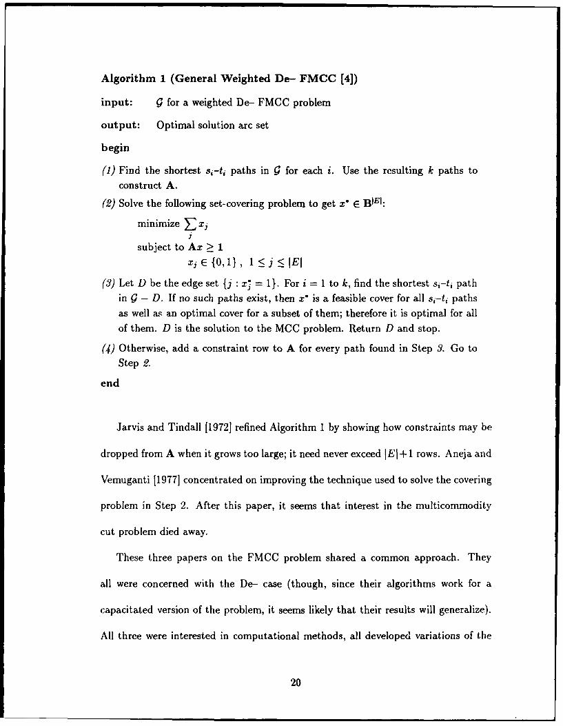
Algorithm 1 (General Weighted De- FMCC [4])

input: g for a weighted De- FMCC problem

output: Optimal solution arc set

begin

(1) Find the shortest si-ti paths in !9 for each i. Use the resulting k paths toconstruct A.

(2) Solve the following set-covering problem to get x* E BIEI:

minimize Xi

subject to Ax > 1Xi E {0, 1} , 1 < j <_ JEI

(3) Let D be the edge set {j : x* = 1}. For i = 1 to k, find the shortest si-ti pathin g - D. If no such paths exist, then x" is a feasible cover for all si-ti pathsas well as an optimal cover for a subset of them; therefore it is optimal for all

of them. D is the solution to the MCC problem. Return D and stop.

(4) Otherwise, add a constraint row to A for every path found in Step 3. Go toStep 2.

end

Jarvis and Tindall [1972] refined Algorithm 1 by showing how constraints may be

dropped from A when it grows too large; it need never exceed IEI + 1 rows. Aneja and

Vemuganti [1977] concentrated on improving the technique used to solve the covering

problem in Step 2. After this paper, it seems that interest in the multicommodity

cut problem died away.

These three papers on the FMCC problem shared a common approach. They

all were concerned with the De- case (though, since their algorithms work for a

capacitated version of the problem, it seems likely that their results will generalize).

All three were interested in computational methods, all developed variations of the

20

same algorithm, and all gave computational experience on test cases. However, none

provided a complexity analysis of the algorithm. None made use of graph theory.

Two basic propositions on multicommodity cuts were published as lemmas in a

paper by Hu on two-commodity flows in 1963 [22]. They are these:

Proposition 1 [Hu, 1963] In a weighted two-commodity multicommodity cut prob-

lem, let C1 be a minimum single-commodity cut separating {sI, s2} from {tI, t2}, and

let C2 be such a cut separating {s 1 ,t 2 } from {t],s 2}. Then the smaller of CI,C2 is a

minimum two-commodity cut. *

Proposition 2 [Hu, 1963] If C is a minimal solution to a full multicommodity cut

problem, then 1? = ! - C has at most k + 1 components. *

The bulk of Hu's paper was on finding feasible flows. It does not seem that the graph-

theoretic approach to multicommodity cuts was pursued beyond this beginning.

3.4 Disjoint Paths

The much-studied disjoint paths problem can be defined as the following decision

problem:

Given a multicommodity flow graph g, are there k disjoint si-ti paths in(DJP) it, one for each commodity?

DJP can also be formulated as a construction problem (find the paths if they exist). It

has edge- and vertex-disjoint cases, and these can be in directed or undirected graphs.

It has received much attention both because of its theoretical interest and because of

its important applications in the design of very large scale integrated (VLSI) circuits.

21

Frank [1990b] has recently published a survey of the state of knowledge for DJP and

some related problems. DJP can also be formulated as a special case of finding integer

multicommodity flows (IMCF). The following subsections give a taxonomy of the

DJP cases and their relationship, review complexity results for DJP, and discuss the

state of knowledge for IMCF, the four basic cases of DJP, and a few of its specialized

versions.

The DJP Cases and their Relationship

The basic distinctions between the DJP problems are made according to whether

the graph is directed or undirected and whether the paths are vertex- or only edge-

disjoint. Using the D/U and V/E codes defined on page 14, the four resulting basic

cases can be called D-V, D-E, U-V, and U-E. Furthermore, there are easy ways to

reformulate a U-E as a U-V and a U-V as a D-V problem [Schrijver, n.d.], and D-V

and D-E problems can be reformulated as each other. In this sense the U-E case

is the easiest and the D-V and D-E cases the hardest. The other shorthand codes

defined on p. 14 can be used to designate restricted versions of the problem.

The Intractability of the DJP Cases

This subsection will summarize the versions of the DJP problem that are known

to be NP-complete. This was recently reviewed by Middendorf and Pfeiffer [1990].

All four basic cases are NP-complete in general, even for planar graphs, even for

grids [Frank, 1990b). In addition, the U-E case remains NP-complete if the graph

is Eulerian [Middendorf and Pfeiffer, 19901, U-V remains NP-complete if 9 is planar

22

and has maximum vertex degree of 3 [ibid.], and D-E remains NP-complete even if

the number of commodities is restricted to two [Fortune, Hopcroft, and Wyllie, 1980].

The Integer Multicommodity Flow Problem

The integer multicommodity flow problem, phrased as a decision problem, is this:

Given a multicommodity flow graph with integer-valued maximum capac-(IMCF) ities defined on each edge, and with integer-valued total flows f; requiredfor each commodity, are there integer-valued flows that are simultaneously

feasible and will sat' f-, every demand?

There is also a correspoi. ag construction problem and a maximum sum-of-integer-

flows problem. The graph can be directed or undirected, so these two basic cases can

be called D-- and U--. If demands and capacities are all 1, then IMCF becomes

the D-E or U-E DJP problem. Other special versions of IMCF correspond to D-V

and U-V DJP. Even, Itai, and Shamir [1976] showed that both basic cases of IMCF

are NP-complete, even for just two commodities and even if all capacities are 1.

(This immediately implies that the U-E and D-E DJP problems are NP-complete

even when 7" is restricted to two sets of parallel edges.) Evans and Jarvis [1979]

found sufficient conditions for the existence of IMCFs, but they are computationally

laborious to evaluate, requiring the comparison of every pair of cycles in the graph.

Most other research on the IMCF problem has concentrated on finding tractable

special cases of undirected planar graphs, which turn out to be cases in which the

maximum flow can be shown to be half-integral. Before discussing these results it

will be convenient to discuss the general cut condition (GCC), which is important for

both the IMCF and DJP problems, as well as for partial multicommodity cuts.

23

The general cut condition is a statement of the obviously necessary condition that

for any edge-cut in a graph, the total flow required between terminals on opposite

sides of the cut must not exceed the capacity of the edges in the cut. In a diLected

problem, it is the capacity of the arcs oriented in the correct direction that counts.

The surplus of a cut is its capacity minus the required flow across it (some reasearchers

call this the free capacity or excess capacity). These concepts apply to a DJP problem

exactly as to IMCF with all demands and capacities equal to 1. For both DJP and

IMCF, many results are of the form of finding cases in which GCC is sufficient as

well as necessary for the existence of a feasible solution. In IMCF, the GCC has been

shown to be necessary and sufficient for U--PBEu* [Okamura and Seymour, 19811

and U--P*Eu* [Seymour, 1981b]. Polynomial algorithms also result immediately

from these results.

The directed case of IMCF has not received the attention that the undirected case

has. Nagamochi and Ibaraki [19891 showed that if a certain kind of class of directed

networks has the max-flow min-cut property, then that class also has the integral

max flow property. These classes are those such that if a network M is in the class (a

network being a directed graph, a set of ordered pairs of terminals, and integer-valued

capacities and demands), then the same network with either a capacity or a demand

decreased by one is also in the class.

Disjoint Paths Case U-E

This is perhaps the most widely studied of the DJP cases. Published results fall

into four broad categories: special cases in which the general cut condition is sufficient

24

as well as necessary; special cases in which GCC plus an additional condition is

necessary and sufficient; special cases in which sufficient conditions have been found:

and polynomial algorithms for the decision or construction problems. A common

thread is the consideration of graphs that are planar, or T-planar, or planar with the

terminals on two faces, or Eulerian when augmented with the (si, ti) demand edges,

or limited to a fixed number of commodities. Consideration of these configurations

cuts across the four categories mentioned earlier, but some configurations find more

application in one than in another.

GCC has been shown to be necessary and sufficient for the existence of disjoint

paths for a variety of conditions when the augmented graph G* is Eulerian. These

include U-EP*Eu* and U-EPBEu* [Seymour, 1981b]; whenever no subgraph can be

contracted to the complete graph on five vertices (K5 ) [Seymour, 1981a]; U-EPEu*

when G can be drawn with all si on one finite face and all ti on another in the

same cyclical order and opposite direction [Schrijver, 1989]; and U-EEu* when the

demand graph R" has a minimum cover of one or two vertices or is a K4 or C5 graph

(circuit on 5 vertices) when parallel edges are replaced by a single edge [Frank, 1990b;

Schrijver, 1991]. (These conditions on 7- can be stated as this: R has neither of the

configurations of Figure 1 as a subgraph [Schrijver, 1991].) Frank has described two

situations in which GCC plus another condition is necessary and sufficient for the

existence of disjoint paths. The first involves an intersection criterion (IC), which

turns out to be always necessary for a feasible solution. Let a tight set be any set

X C V such that the cut-set F(X) has zero surplus. The IC states that for any

25

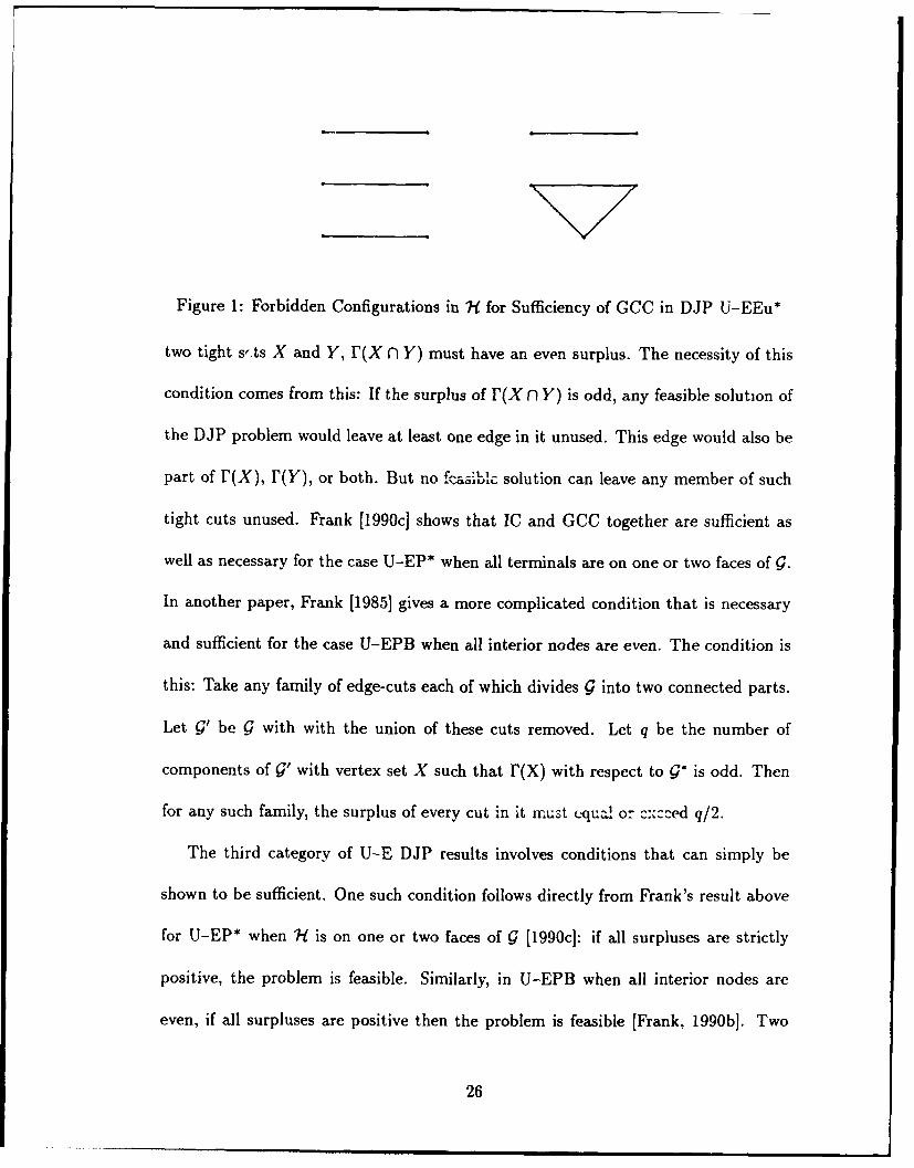
Figure 1: Forbidden Configurations in 'H for Sufficiency of GCC in DJP U-EEu*

two tight s-,ts X and Y, F(X n Y) must have an even surplus. The necessity of this

condition comes from this: If the surplus of r(X n Y) is odd, any feasible solution of

the DJP problem would leave at least one edge in it unused. This edge would also be

part of F(X), F(Y), or both. But no fcasiblc solution can leave any member of such

tight cuts unused. Frank [1990c] shows that IC and GCC together are sufficient as

well as necessary for the case U-EP* when all terminals are on one or two faces of G.

In another paper, Frank [1985] gives a more complicated condition that is necessary

and sufficient for the case U-EPB when all interior nodes are even. The condition is

this: Take any family of edge-cuts each of which divides g into two connected parts.

Let g' be g with with the union of these cuts removed. Let q be the number of

components of 9' with vertex set X such that F(X) with respect to 9* is odd. Then

for any such family, the surplus of every cut in it must equa! or c=ceed q/2.

The third category of U-E DJP results involves conditions that can simply be

shown to be sufficient. One such condition follows directly from Frank's result above

for U-EP* when R- is on one or two faces of G [1990c]: if all surpluses are strictly

positive, the problem is feasible. Similarly, in U-EPB when all interior nodes are

even, if all surpluses are positive then the problem is feasible [Frank, 1990b]. Two

26

more results for planar graphs when all surpluses are nonnegative and even are due to

Okamura [1983]: if there are at most two faces such that the source and sink for each

commodity are on one of them, the problem is feasible; if one set of terminal pairs

is on one face and the rest of the pairs share a common vertex on that same face,

the problem is also feasible. Some other sufficiency results are even more specialized.

Frank [1990b] surveys a series of results of the following form: for some integer p and

k, if a graph is p-edge-connected, then any k-commodity DJP U-E problem defined

on it is feasible regardless of which vertices are the terminals.

The last major category of results is that of decision or construction algorithms.

Sometimes the proof of a sufficiency result can be used directly in a polynomial

algorithm. This is the case for Frank's special cut condition for the U-EPB case with

all interior nodes even (19851. Seymour [1980al developed a polynomial algorithm

for the U-E2 problem; it can also be used as the basis for a construction algorithm.

Based on the work of Frank [1985, 1990b], Becker and Mehlhorn [19861 have offered

both decision and construction algorithms for U-EPB with all vertices even, and also

for U-EPBEu*. Middendorf and Pfeiffer [1990] have shown that U-EP in general is

polynomial if the terminals are on a bounded number of faces of g.

Besides these direct results for variations on the U-E problem, others could be

derived from results for the U-V, D-V, or D-E cases. All that required is that any

special requirements (e.g. planarity) persist after transforming the problem.

Disjoint Paths Case U-V

The problem of finding vertex-disjoint paths in an undirected graph has not been

27

investigated in as many variations as the corresponding edge-disjoint problem. The

common restrictions are to planar graphs, perhaps with the terminals on one or two

faces, and to two-commodity problems. U-VP results have recently been surveyed by

Seb6 [1990]. The general cut condition (GCC) applies as a necessary condition to U-V

in a modified form: no subset of t vertices can separate more than I terminal pairs.

Necessary and sufficient conditions (including GCC) have been found for two cases.

These will be discussed in this subsection, followed by some sufficient conditions that

have been found and some results on algorithms.

The first necessary and sufficient condition was found for the U-VPB case by

Robertson and Seymour [1986]. The condition is GCC plus the supply graph g

being cross-free, i.e. having the terminals for no two commodities in interleaved order

s1 ,sj,Ii,tj. Since in a planar graph vertex-disjoint paths can never cross, this is

obviously a necessary condition. The same investigators also found necessary and

sufficient conditions for the general U-VP problem [Robertson and Seymour, 1988],

but the conditions do not seem to lend themselves to succinct statement. They

correspond to the graph being "big enough" and to terminals of different pairs being

"far enough apart."

Research on special sufficient conditions for the existence of disjoint U-V paths

has been limited to finding the level of connectivity in a graph at which any given

pairs can be connected with disjoint paths. Some results of this sort have been given

by Watkins [1968], Larman and Mani [1970], and Shiloach [1980].

The last category of results concerns the development of practical or polynomially

28

bounded algorithms for the U-V DJP problem. This has followed a fairly straight-

forward development. First Pert and Shiloach [19781 gave construction algorithms for

two commodities in planar graphs. Shiloach [19801 and Seymour [1980a] then indepen-

dently showed that the general U-V2 problem is polynomial. Robertson ai. ' ,nour

[1985] proved that U-VPk is polynomial for any fixed number k of commodities, but

the proof did not yield a practical algorithm (the degree of the polynomial exceeds

101" for k = 4). Shortly afterwards, the same writers showed that U-VP is poly-

nomial for arbitrary k if ;al terminals are on one or two faces [1986]; this yielded an

easy greedy algorithm for the U-VPB case. Recently, Schrijver [19901 has proved the

generalization that U-VP is polynomial if the terminals are on any bounded number

of faces of g. Also, Middendorf and Pfeiffer [1990] have shown that a resLrictedt U-V

problem is polynomial if and only if some planar graph is excluded from appearing

as a subgraph in the restricted class.

Disjoint Paths Cases D-E and D-V

Published results for disjoint paths in directed graphs are so few that it is con-

venient to discuss the edge-disjoint and vertex-disjoin* 'ases together. In any case.

either general problem can be reformulated as the other by splitting nodes, as already

mentioned. There are no known situations in which the general cut condition is suf-

ficient by itself. There is one situation in which a necessary and sufficient condition

is known. A few sufficiency results and a couple of polynomial algorithms have been

published.

Very recently, Ding, Schrijver, and Seymour [1992] proved that a D-VPB problem

29

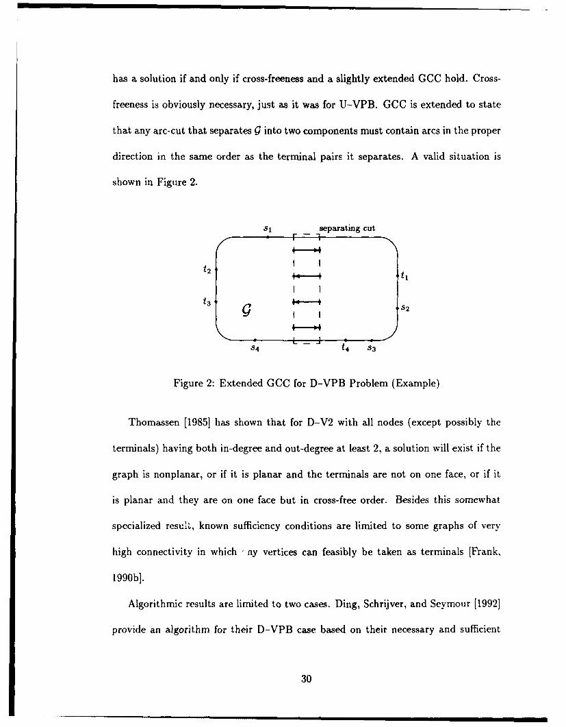
has a solution if and only if cross-freeness and a slightly extended GCC hold. Cross-

freeness is obviously necessary, just as it was for U-VPB. GCC is extended to state

that any arc-cut that separates Q into two components must contain arcs in the proper

direction in the same order as the terminal pairs it separates. A valid situation is

shown in Figure 2.

81 separating cut

F4- q1

I It2I I

t 3 i S

84 - t 4 83

Figure 2: Extended GCC for D-VPB Problem (Example)

Thomassen [19851 has shown that for D-V2 with all nodes (except possibly the

terminals) having both in-degree and out-degree at least 2, a solution will exist if the

graph is nonplanar, or if it is planar and the terminals are not on one face, or if it

is planar and they are on one face but in cross-free order. Besides this somewhat

specialized result, known sufficiency conditions are limited to some graphs of very

high connectivity in which ny vertices can feasibly be taken as terminals [Frank,

1990b].

Algorithmic results are limited to two cases. Ding, Schrijver, and Seymour [1992]

provide an algorithm for their D-VPB case based on their necessary and sufficient

30

conditions for it. The other case is for graphs without directed circuits: Perl and

Shiloach [1978] give a polynomial construction algorithm for D-V2, and Fortune,

Hopcroft, and Wyllie [1980] show that the D-Vk decision problem in such a graph is

polynomial for any fixed integer k.

Specialized Versions of the Disjoint Paths Problem

There are a few frequently-studied special variations on the disjoint paths problem.

These are more distantly related to the multicommodity cut problem, so they do not

need a detailed treatment here. First is finding not just one path between each

terminal pair but as many as possible; this is reviewed by Frank [1990b]. Second is

homotopic routing, i.e. finding exact paths once one is given a general routing around

certain "holes" in the space in which the graph in embedded. This is an important

practical problem in VLSI circuit design, and has been reviewed by Frank [1990a],

Frank and Schrijver [1990], and Schrijver (1990]. The third variation is also of special

application to VLSI circuit design. This is the problem of disjoint paths in a grid:

circuit chips often have a grid-based design structure. The terminals in a grid are

often taken to be on the boundary. Mehlhorn and Preparata [1986], Lai and Sprague

[1987], and Suzuki, Ishiguro, and Nishizeki [1990] are examples of this line of research.

31

4 GENERAL RESULTS

This chapter contains some simple results of a general nature that will be used in

subsequent chapters. It consists of three sections. The first concerns the relationship

between full multicommodity cuts and multiterminal cuts. The second gives two

lemmas on partial multicommodity cuts. The third describes some multicommodity

cut problems that can immediately be seen to be intractable based on others' work.

We assume throughout the paper that g is a connected graph.

4.1 Full Multicommodity Cuts and Multiterminal Cuts

The multiterminal cut problem was defined in Section 3.2 as the problem of finding

the smallest set of edges in a multiterminal graph that separates each terminal from all

of the others. Clearly a minimal multiterminal cut for k terminals will separate Q into

exactly k components: there must be one for each terminal, and an edge connecting

a component with no terminal to any other component would be superfluous in the

cut. Define an i-way multiterminal-separation problem as this: given a multiternmnal

graph ! and an i-partition of its terminal set T, find the smallest set of edges that

will separate each element of the partition from all of the others (without necessarily

leaving each set in one component). Obviously, a multiterminal-separation problem

can be reduced to a multiterminal cut problem by introducing an extra terminal for

every element of the partition and connecting it to each of the corresponding members

by a large number of parallel edges. There is an important relationship between a full

multicommodity cut problem and certain multiterminal-separation problems that it

induces. This relationship will be discussed next.

Any minimal FMCC will separate g into components, which in turn induce in the

terminal set T a partition with the property that si and t, are in different sets for all i.

Call any partition of a multicommodity terminal set a feasible partition if it has this

property. Clearly an optimal FMCC is also the minimum multiterminal-separation

cut for the partition of T that it induces. This leads to the following lemma.

Lemma 1 In a full multicommodity cut problem, any minimum-cardinality i-way

multiterminal-separation cut over all feasible i-partitions, 2 < i < k + 1, is an optimal

solution.

Proof: Such a cut is clearly a feasible solution. Suppose there is a feasible FMCC

C that has smaller cardinality than any of these multiterminal-separation cuts. It

cannot induce a partition of T into fewer than k + 2 sets. By Proposition 2, it cannot

be optimal. a

Define a supreme cut in an undirected full multicommodity cut problem to be any

multiterminal-separation cut using a feasible 2-partition. A supreme cut is always

feasible but not necessarily optimal. Proposition 1 in Chapter 3 states that for k = 2.

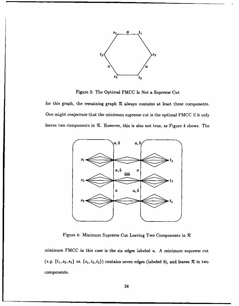
the smallest supreme cut is the optimal FMCC. This is not true for k > 3, as can be

seen in the graph in Figure 3. Every 2-partition of the terminals yields a supreme cut

of at least four edges, but the optimal FMCC consists of the three edges a. Note that

33

s1_ a t

t3 S2

S3 t2

Figure 3: The Optimal FMCC Is Not a Supreme Cut

for this graph, the remaining graph 7Z always contains at least three components.

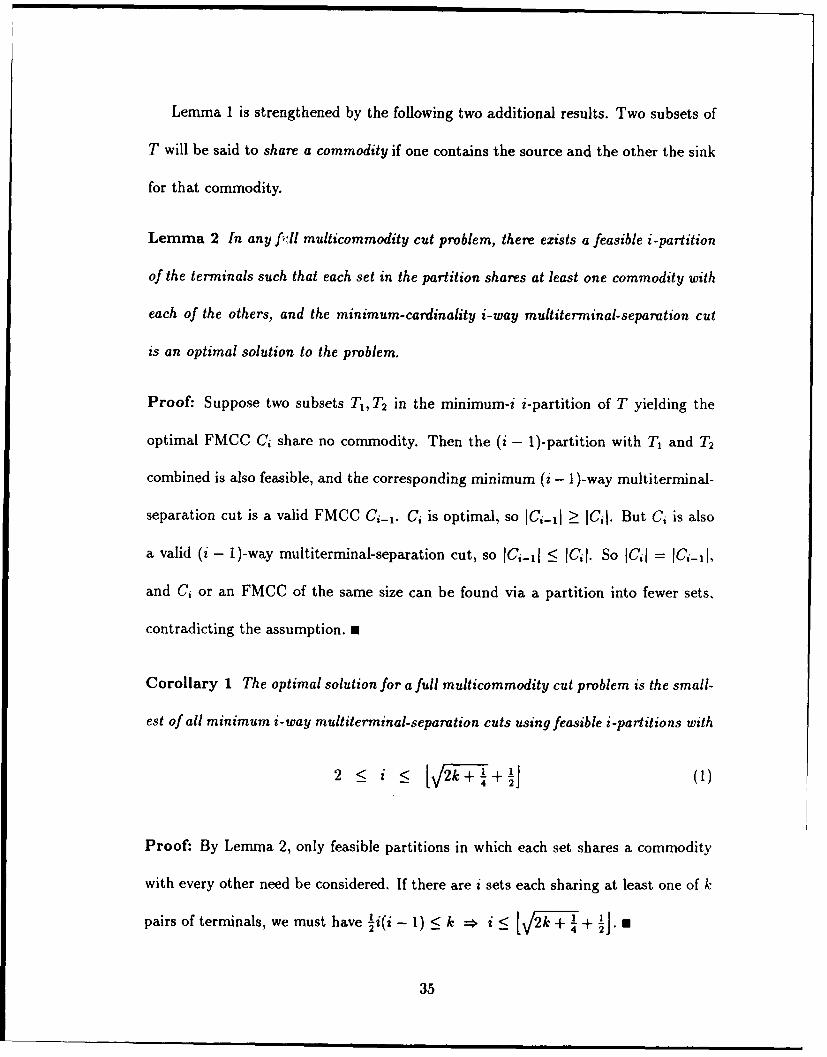
One might conjecture that the minimum supreme cut is the optimal FMCC if it only

leaves two components in XZ. However, this is also not true, as Figure 4 shows. The

a , 6" , a , b I

a, b b a

S2 t3

a a,b

S53

Figure 4: Minimum Supreme Cut Leaving Two Components in R

minimum FMCC in this case is the six edges labeled a. A minimum supreme cut

(e.g. {ItI,S 2 ,8 3 } VS. {S 1 , t 2 , t 3 }) contains seven edges (labeled b), and leaves 'R in two

components.

34

Lemma 1 is strengthened by the following two additional results. Two subsets of

T will be said to share a commodity if one contains the source and the other the sink

for that commodity.

Lemma 2 In any fril multicommodity cut problem, there exists a feasible i-partition

of the terminals such that each set in the partition shares at least one commodity with

each of the others, and the minimum-cardinality i-way multiterminal-separation cut

is an optimal solution to the problem.

Proof: Suppose two subsets TI, T 2 in the minimum-i i-partition of T yielding the

optimal FMCC Ci share no commodity. Then the (i - 1)-partition with T1 and T2

combined is also feasible, and the corresponding minimum (i - 1)-way multiterminal-

separation cut is a valid FMCC Ci- 1. Ci is optimal, so IC,-I Ž__ IC2I. But Ci is also

a valid (i - 1)-way multiterminal-separation cut, so 1Cj-11 • IC,!. So lC j = IC,-1I,

and Ci or an FMCC of the same size can be found via a partition into fewer sets,

contradicting the assumption. a

Corollary 1 The optimal solution for a full multicommodity cut problem is the small-

est of all minimum i-way multiterminal-separation cuts using feasible i-partitions with

2 < i < 2

Proof: By Lemma 2, only feasible partitions in which each set shares a commodity

with every other need be considered. If there are i sets each sharing at least one of k

pairs of terminals, we must have .i(i - 1) < k => i < [2k+ 1j' + .

35

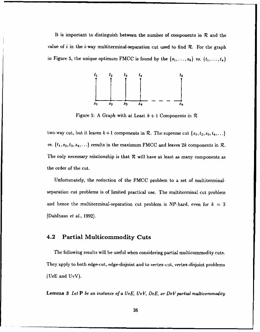
It is important to distinguish between the number of components in 1R and the

value of i in the i-way multiterminal-separation cut used to find R. For the graph

in Figure 5, the unique optimum FMCC is found by the {sl,. . . ,sAJ vs. {t1,... ,tkl

t, t 2 t3 t4 tk

S1 S 2 83 84 Sk

Figure 5: A Graph with at Least k + 1 Components in 1Z

two-way cut, but it leaves k + 1 components in RZ. The supreme cut {sI, t2, s 3, t 4 ,. ..

VS. {tlS 2,t,3S 4,.. .} results in the maximum FMCC and leaves 2k components in 1Z.

The only necessary relationship is that 1R will have at least as many components as

the order of the cut.

Unfortunately, the reduction of the FMCC problem to a set of multiterminal-

separation cut problems is of limited practical use. The multiterminal cut problem

and hence the multiterminal-separation cut problem is NP-hard, even for k = 3

[Dahlhaus et al., 19921.

4.2 Partial Multicommodity Cuts

The following results will be useful when considering partial multicommodity cuts.

They apply to both edge-cut, edge-disjoint and to vertex-cut, vertex-disjoint problems

(UeE and UvV).

Lemma 3 Let P be an instance of a UeE, UvV, DeE, or DvV partial multicommodity

36

cut problem, and let Jr and J,+1 be minimum interjacent sets leaving r and r + 1

disjoint paths, respectively. Then IJrl > IJtr+1 + 1.

Proof: In R,. = 9 - J. no more than r disjoint si-ti paths can be found. For any

x E J,, consider 1?' = G - (Jr - {xJ). No more than r + 1 disjoint paths can be

found in V7', sincc at most one additional disjoint path can be drawn through the

single added element x, which has in effect been removed from Jr and added to lZr.

So J, - {x} is a feasible interjacent set for leaving r + 1 disjoint paths, and IJ.I - 1

is an upper bound on IJr+11. n

Lemma 4 Let P be an instance of a UeE, UvV, DeE, or DvV partial multicommodity

cut problem, and let J be a minimal interjacent set leaving at most r disjoint paths.

Then exactly r disjoint si-ti paths can be drawn in R = g - J.

Proof: If J is feasible then no more than r paths can be drawn in R. Suppose fewer

than r paths can be drawn. If any element of J is deleted from the interjacent set,

and so added to 7"., then at most one additional disjoint path is made possible. So J

without this element is still feasible, contradicting its minimality. s

4.3 Two Propositions on Intractability

This section concludes the chapter by giving two propositions on the intractability

of large classes of multicommodity cut problems. The first is on full edge-cuts in

undirected graphs, while the second covers a variety of partial cut problems.

The first proposition makes it unlikely that Proposition 1 can be extended to cover

more than two commodities.

37

Proposition 3 The full multicommodity edge-cut problem in general graphs is

NP-hard for k > 3, even for k fixed.

Proof: A three-terminal cut problem can be reduced to a multicommodity cut with

k = 3 by identifying one of the three terminals as s, and t2 , another as S2 and t3 , and

the third as t, and s3. The multiterminal cut problem is NP-hard even for k fixed

at 3 [Dahlhaus et al., 19921. .

The second proposition is based on the fact that a partial multicommodity cut

problem cannot be easier than the corresponding disjoint paths problem. A disjoint

paths decision problem with k, commodities can be reduced to a PMCC problem

with k, + 1 commodities and r = k, by attaching to the graph a simple structure

with a new source and sink that can be disconnected by the removal of one structure

element. The solution to such a PMCC cannot be of cardinality more than 1. If it is

empty, then the answer to the DJP decision problem is "no," otherwise the answer

is "yes." Since many versions of the DJP problem are NP-hard, the corresponding

versions of the PMCC problem are also intractable.

Proposition 4 All cases of the partial multicommodity cut problem are NP-hard,

and they remain NP-hard even under the following restrictions:

"o UeE, UvV, UeV, and UvE on an induced subgraph of a grid with r = k - 1

"o UvV and UeV on a planar graph with maximum vertex-degree of 3 and r = k- I

"o DvV and DeV on a grid with r - k - 1

"o DeE and DyE with k fixed and r = 2

Proof: NP-hard restricted versions of the disjoint paths problem (see Section 3.4)

can be reduced to these problems, as outlined in the paragraph above. a

38

5 FULL MULTICOMMODITY CUTS IN

PLANAR GRAPHS

This chapter discusses various cases of the Ue-P full multicommodity cut problem:

the supply graph Q = (V, E) is taken to be undirected and planar, and a minimum set

of edges C C E is sought such that 9 - C will contain no si-ti paths. In Section 5.2

an algorithm for the T-planar case Ue-PB is presented; the algorithm is polynomially

bounded if the number of commodities k is fixed. If the terminals are not restricted

to the boundary of !g then the problem becomes more complicated. In Section 5.3

a polynomial algorithm for the Ue-Pk case with k = 3 is presented. Sections 5.4

and 5.5 consider the problem when k is part of the input. If k is not fixed then the

T-planar FMCC problem becomes NP-complete even under some strong restrictions

on G; the proofs for this are the main content of Section 5.4. However, if the terminals

are in non-crossing order (Ue-P*BN) then a polynomial algorithm is again possible,

and such an algorithm is developed in Section 5.5.

The algorithms in this chapter mostly depend on a correspondence between edge-

cuts in g and trees in a modification of the geometric-dual of G. This modified dual

will be called GDm; the next section describes how G D, is constructed and proves

the necessary relationships. The next section also applies the method to the Ue-PB

multiterminal cut (MTC) problem. This has three purposes. It illustrates the use

of the modified dual in a problem that is a bit simpler than the FMCC problem. It

shows that an important special case of the planar MTC problem is polynomially

bounded, even though the general problem is NP-complete [Dahlhaus et al., 1992].

Finally, since an MTC problem can be reformulated as an FMCC problem with co-

located terminals, it provides a polynomial algorithm for a special case of the Ue-PB

FMCC problem.

5.1 The Modified Dual g"f and the Ue-PB MTC Problem

The modified dual graph gDm is formed in the following way. Let g be a T-planar

graph with terminals t1 , t2,. .. , tk numbered in order clockwise around the boundary.

Form the geometric-dual gD, but split the dual vwrtex corresponding to the infinite

face into k vertices, one for each of the k paths into which the boundary of G is

partitioned by the terminals. Call these k vertices the separation-vertices of GDm

and label them al, a2,..., ak in clockwise order around the boundary of gDm in such

a way that ao corresponds to the path from ti-. clockwise to ti, and al corresponds

to the path from tk clockwise to tj in G (see Figure 6). This is the modified dual

graph ODm = (vDm, EDm). Note that it is planar, and that there is a one-to-one

correspondence between the edges of G and those of gDm.

We will use certain conventions when discussing G and gDm,. The notation [ti, tj]

means the set of terminals in ! from ti clockwise through tj; the set [ai, aj] is similarly

defined in gDm. If i is not in {1,.f k} then ai = ai0 k, and similarly for ti. If C

is a set of edges in g then CDm is the set of corresponding edges in GDm (not the

40

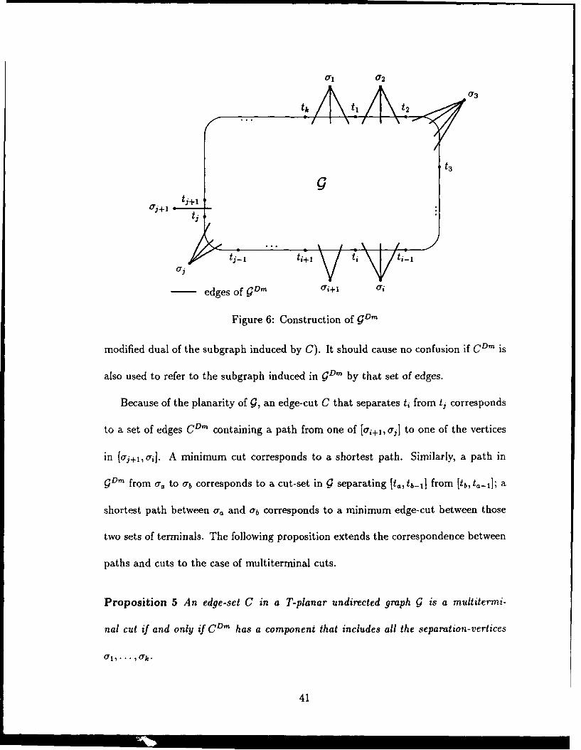
01 o02

t3

ti+l '

'j tj ,

a t,.i- ti+1 ii \ l/ ti-m

edges of gDm ati+1 ori

Figure 6: Construction of gDm

modified dual of the subgraph induced by C). It should cause no confusion if C0 D is

also used to refer to the subgraph induced in gDm by that set of edges.

Because of the planarity of 9, an edge-cut C that separates ti from tj corresponds

to a set of edges CD, containing a path from one of [0.i+i, aj] to one of the vertices

in (aj+,, ail. A minimum cut corresponds to a shortest path. Similarly, a path in

gDm, from oa to Ub corresponds to a cut-set in ! separating [ta, tb-1] from [tb, ta-l]; a

shortest path between oa and 0.b corresponds to a minimum edge-cut between those

two sets of terminals. The following proposition extends the correspondence between

paths and cuts to the case of multiterminal cuts.

Proposition 5 An edge-set C in a T-planar undirected graph g is a multitermi-

nal cut if and only if CD' has a component that includes all the separation-vertices

41

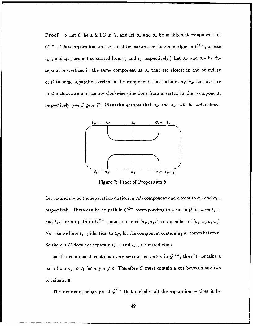
Proof: •:, Let C be a MTC in g, and let o' and 0b be in different components of

CD,. (These separation-vertices must be endvertices for some edges in CDm, or else

ta-l and tb.1 are not separated from t. and tb, respectively.) Let '., and Cat, be the

separation-vertices in the same component as oa that are closest in the bouxndary

of Q to some separation-vertex in the component that includes ab; C'a and Cat, are

in the clockwise and counterclockwise directions from a vertex in that component.

respectively (see Figure 7). Planarity ensures that oa, and Ct,, will be well-define,.

a'-1 Ca' Caa l" at#

t b' ab' ab ab" tb1-I.

Figure 7: Proof of Proposition 5

Let ob' and ab,, be the separation-vertices in ab'S component and closest to C'a and Cat,

respectively. There can be no path in C'm corresponding to a cut in g between t,,_1

and ta", for no path in CD, coniects one Of [oC', Cat' I to a member of C'a"+•1, oCat1].

Nor can we have ta,_1 identical to te,,, for the component containing Orb comes between.

So the cut C does not separate ta'-1 and tall, a contradiction.

. If a component contains every separation-vertex in gDm, then it contains a

path from o' to 06 for any a =A b. Therefore C must contain a cut between any two

terminals. m

The minimum subgraph of gDm that includes all the separation-vertices is by

42

definition the Steiner tree in gDm on those vertices. Hence we get the following

corollary:

Corollary 2 An edge-set C is a minimum MTC in a T-planar graph G if and only

if CD, is a Steiner tree on the separation-vertices of gD*.

The separation-vertices in gDm are on its boundary, and the problem of finding the

minimum-edge-weight Steiner tree in a planar graph on a subset of its boundary

vertices is known to be polynomial [Provan, 1988; Erickson, Monma, and Veinott.,

1987; Provan, 1983]. Since a weighted version - ! can be obtained from G in

polynomial time, we also get the following:

Corollary 3 The weighted multiterminal cut problem in T-planar undirected graphs

is polynomially bounded.

As already noted, the planar MTC problem is NP-complete if the terminals are al-

lowed to be anywhere in G [Dahlhaus et al., 1992].

These results suggest an algorithm 'or solving a weighted Ue-PB MTC problem.

The method is to form Gm, then use Provan's algorithm [1988] to find a Steiner

tree on it. The major work would be finding the tree, which would be O(a + f 2 k2 ).

where a is the work required to find the distance between each pair of vertices in G D,

(a = f 2 [Frederickson, 1987]) and f is the number of vertices in that graph (i.e. the

number faces in G).

5.2 The Ue-PBk FMCC Problem

Next consider the problem of finding a weighted full multicommodity cut in a

43

T-planar undirected graph. An algorithm is developed that is polynomially bounded

for any fixed number of commodities k. (It will be shown later that the problem is

NP-hard if k is part of the input; see Section 5.4.) The algorithm is an adaptation

of Provan's method for finding Steiner trees (1988]; it operates on the modified dual

graph gDm

The modified dual g°m is defined for a T-planar multicommodity flow graph

just as it was for a multiterminal graph in the previous section. It is the normal

geometric-dual with the vertex corresponding to the infinite face of G split into one

separation-vertex for each path between consecutive terminals in the boundary of

g. The only difference between the FMCC and MTC cases is in the labeling of the

separation-vertices, and comes from the fact that in g the terminal set T is the union

of a set of sources {s 1 ,. . ,skl and a set of sinks {tl, .. . , tk}. These sets may occur

in any order around the boundary of g, and two or more terminals can be co-located

(except the source and sink of one commodity). Label the distinct terminals in g

from a, to a, in clockwise order around the boundary from an arbitrary start. Note

that z = 2k if none of the terminals coincide; otherwise z < 2k. Then gD' as already

defined will have exactly z separation-vertices; label them likewise from a, clockwise

to a,, with al falling between a, and a, (see example in Figure 8). Each edge in gD,a

has the same weight as the corresponding edge in g.

(It will turn out to be awkward if a terminal is encountered twice in tracing the

boundary of !. For this reason, if a terminal is an articulation vertex, it should be

displaced to the end of an infinite-weight edge before constructing g!D'. This has

44

a/o1,'-. o.a / .I~~~3 S4 a

t 4 a3

0----o go_,

bedonefr \ia1 i Figure 8.)

throuh a4aa6 \ / t3 0t• \

t2 t gz is l te h

0`6S---g 0---o gDm

Figure 8: Example of gDm for an MCF Graph

been done for sulc am in Figure 8i)

The following definitions are needed to deal with the distribution of terminals

around the boundary of i :

lai, aj] from o ft o st we di terminal vertices ind from an clockwise (2)through aj

IKi the set of commodities with a terminal at a; (3)

In Figure 8, K2 f 3,4}. (An index i of ai that is incremented or decremented out

of the range 11,. .. , z} is to be taken modulo z.) Now we can extend the relationship

between cuts in !9 and trees in gore to the case of multicommodity flow graphs.

Proposition 6 In a weighted T-planar multicommodity flow graph !9, a minimum

full multicommodity edge-cut C will correspond to a forest in gDm, and each tree in

that forest will be a Steiner tree on some subset of the separat ion-ve rt ices.

Proof. Note that si is separated from tj in !g by a set of edges C if and only if C°m

includes a path from a,, to ab, where a. lies between si and tj (reckoned clockwise) and

45

ab lies similarly between ti and si. Now if C is an FMCC, then CD, must contain

at least two separation-vertices; otherwise the boundary of g will connect all the

terminals in R. If CD, is not a forest, then it contains a circuit. But every circuit in

gDm encloses only nonterminals in g, so one of the edges corresponding to the circuit

could be deleted from C without connecting any terminals in R, and the cut would

not be minimum-weight. Furthermore, CDm can have no degree-1 vertices except

separation vertices, for the edge on such a vertex would correspond to a superfluous

edge in C. So CDm is a forest and all its degree-1 vertices are separation-vertices. It

remains only to show that every tree in it is in fact a minimum-weight Steiner tree

on the separation-vertices it contains.

Let one of these trees contain the set of separation-vertices {ab, .. ,..., a., oru,

occuring in the given order clockwise around GD,,. Then the corresponding edge set

in ! (which is a subset of the FMCC C) serves to separate the terminal vertex sets

[ay, ab-l], [ab, ac-1], ... , [as,, ayi, each from the others. But the minimum-weight

Steiner tree on those separation-vertices will accomplish exactly the same thing, and

at minimum cost. Therefore the tree must be a minimum-weight Steiner tree on its

separation-vertices, as required. *

(This proposition can also be proved directly from Lemma 1 on p. 33 and Corollary 2

on p. 43.) From this point a tree in gDm will be referred to as separating a commodity

when the tree's edge-set CDm corresponds to a set of edges C in g that separates that

commodity's source from its sink.

As a consequence of Proposition 6 we have the following:

46

Proposition 7 The weighted full multicommodity edge-cut problem in a T-planar

graph is polynomially bounded for any fixed number of commodities k.

Proof: Proposition 6 showed that the optimal FMCC in g corresponds to Steiner

trees on subsets of the separation-vertices in gDm. If k is fixed then the number of

separation-vertices is bounded at 2k, and the number of possible subsets of them is

also bounded. So all that is required to solve the problem is to evaluate a bounded

number of minimum-weight Steiner tree problems and pick the smallest-weight tree or

combination of trees that separates all commodities. Since the Steiner tree problem

in a weighted T-planar graph is polynomial, and checking whether a given set of

trees separates all commodities is polynomial, this restricted FMCC problem is also

polynomial. n

(This proposition can also be proved directly from Lemma 1 on p. 33 and Corollary 3

on p. 43.) Of course, it can be expected that there are algorithms that are much

better than examining all possible Steiner trees. We now develop one that runs in

time O(f 2 ), where f is the number of faces in g or vertices in gDm, if k is fixed.

The method used in the algorithm for the Ue-PB FMCC problem is adapted

from Provan's method of finding a Steiner tree in a T-planar graph [1988]. The

approach is to find the minimum-weight forest of Steiner trees in G°Dn that separates

all commodities. It relies on the fact that if any Steiner tree in GD, is partitioned into

two pieces, the separation-vertices in the two pieces cannot be in interleaved order

around the boundary of gDm. Also, the separation-vertices on any two separate trees

in g•Dm cannot be interleaved.

47

Some definitions will be needed for the algorithm.

term[Gi, aji the set of commodities with at least one termi- (4)nal falling between ao and aj, i.e. in [ai,a-.i](term[a,,ai] =_ €)

comm[ai, ai] the set of commodities with both terminals falling (5)between ao and aj (comm[ai, ari] =_ )

Thus term[a, aj] is the union of Ki clockwise through Kj1.; comm[a, aj] is the set

of commodities represented twice in Ki through Kj1.. In Figure 8, term[a 2, a6] =

{1,2, 3, 4} and comm[k 2, "6] = {3}. A set of edges in gDm (or the subgraph induced

by them) will be called a [ao, aj]-feasible subforest if it corresponds to a subset of

a minimal FMCC in g, separates all commodities in comm[ai, aj, and contains no

separation-vertices that are not in [ai, Uj].

Two functions on gDm will also be needed. The first is:

T[a,, Ob] =- weight of a minimum-weight [U., Ub]-feasible subforest (6)with a, and ab in the same component

Thus T[ua, ab] is the weight of an optimal tree that is on aa, ab, and possibly some of

[a, ab] - {Ia,Ob}, plus the weight of all other trees on subsets of [aa, ab] - {Ia,ab}.

For the second function, suppose we know that some optimal forest has [aj, ai and

ai, aj] - {ji, aj} in different components, and let K be the subset of commodities

in term[aj,Ga]\comm[aj,ai] that are not separated by the components on [ajai].

For instance, if the only trees on members of [oj,ai] are one that contains aj and

ac and another that contains ad and a, (aG, ad E [aj,aiG), then the commodities in

term[Ga, Gd]\comm[aj, ai] are not separated by any tree on [aj, aGl, and term[aG, ad] n

48

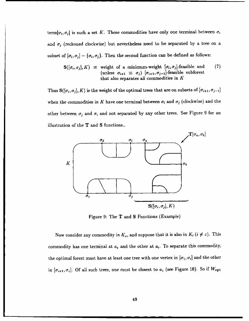
term[o'i, oj] is such a set K. These commodities have only one terminal between a,

and aj (reckoned clockwise) but nevertheless need to be separated by a tree on a

subset of [fr, ari - {ja, oj}. Then the second function can be defined as follows:

S([ua,,jj,K) = weight of a minimum-weight [, aioj]-feasible and (7)(unless ar+4 =_ cj) [ari+1,.aj -]-feasible subforestthat also separates all commodities in K

Thus S([ai, aj], K) is the weight of the optimal trees that are on subsets of [a,+ , Oj-1]

when the commodities in K have one terminal between ai and cri (clockwise) and the

other between aj and ri and not separated by any other trees. See Figure 9 for an

illustration of the T and S functions..

T [or., Ub]

ad ori a,

K 1b

Soac oo] K

Figure 9: The T and S Functions (Example)

Now consider any commodity in K., and suppose that it is also in Ki (i # z). This

commodity has one terminal at a_ and the other at ai. To separate this commodity,

the optimal forest must have at least one tree with one vertex in [a,, Tri] and the other

in [ai+I, o7z]. Of all such trees, one must be closest to a. (see Figure 10). So if Wopt

49

01P 4i1

0rq

S(f[q, 0,p], 4 ) T[P, adq]

Figure 10: T and S Functions in an Optimal FMCC (Example)

is the weight of the optimal FMCC, we can write

Wop t= min {T[ap,oq]+S([aq,ap],0)} (8)(9p,,q)EQ

where

or a. {(',q: Oap E [(al, ail, aq E [f'i+i,O01.1,

T and S can be calculated via recursive formulas, which will now be developed.

A recursive formula for S([a, a,], K). S need not be defined if [ai, aj] contains

only one vertex (i.e. i = j). Suppose (ai,,a] contains only two or three separation-

vertices. Then [ai+i,aj-1] contains at most one separation-vertex, and there can be

no Steiner tree on it. This gives

S([aj,ail, K) = 0 if [ai,ajl < 3 and K n term[ai,oj] = (9)comm[ai, a3 ] =

S([a1, aj],K) = oo if j[a_,ajj< 3, and K n term[a,,aj) or (10)comm[ai, a,] is nonempty

50

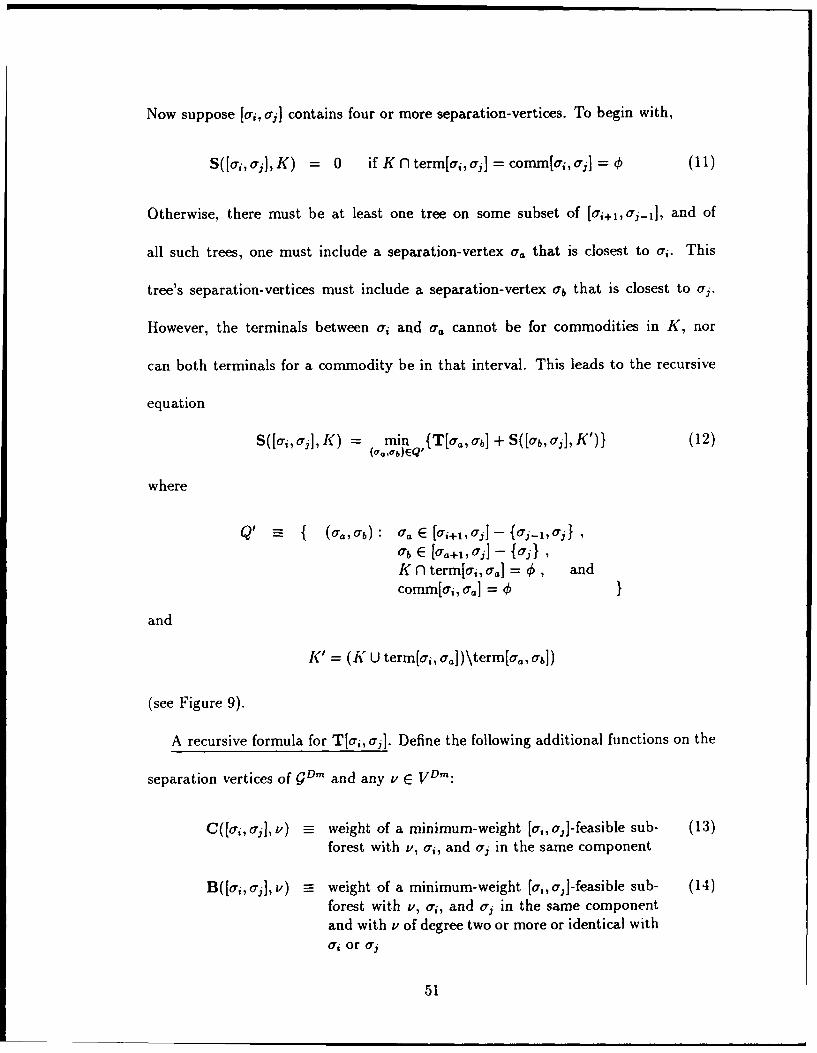
Now suppose [ai, aji contains four or more separation-vertices. To begin with,

S([ai, aj],K) = 0 if K nterm[a,,aj] = comm[ao, j] = 0 (11)

Otherwise, there must be at least one tree on some subset of [a,+i,0j-1], and of

all such trees, one must include a separation-vertex ao. that is closest to a:. This

tree's separation-vertices must include a separation-vertex ab that is closest to aj.

However, the terminals between ai and a. cannot be for commodities in K, nor

can both terminals for a commodity be in that interval. This leads to the recursive

equation

S([a1 , aj, K) = amin {T[a0 , ab] + S([ab, aj], K')} (12)(u 0 ,ab)EQ'

where

Q' --- { (aa,ab): a. E [fa,+i, - {a- -, a} I0Ub E [a01+ 1,,ai - jai} ,

K n term[ai, = a , andcomm[a,, a]=

and

K' = (K U term[ai, a0 ])\term[a0 , ab])

(see Figure 9).

A recursive formula for T[a,, aj]. Define the following additional functions on the

separation vertices of Dm' and any v E VDm:

C([ou, aj],v) weight of a minimum-weight [ai, a3j-feasible sub- (13)forest with v, aj, and aj in the same component

B([a, aj1], v) weight of a minimum-weight [ai, aj]-feasible sub- (14)forest with v, a1 , and aj in the same component

and with v of degree two or more or identical withoai or aj

51

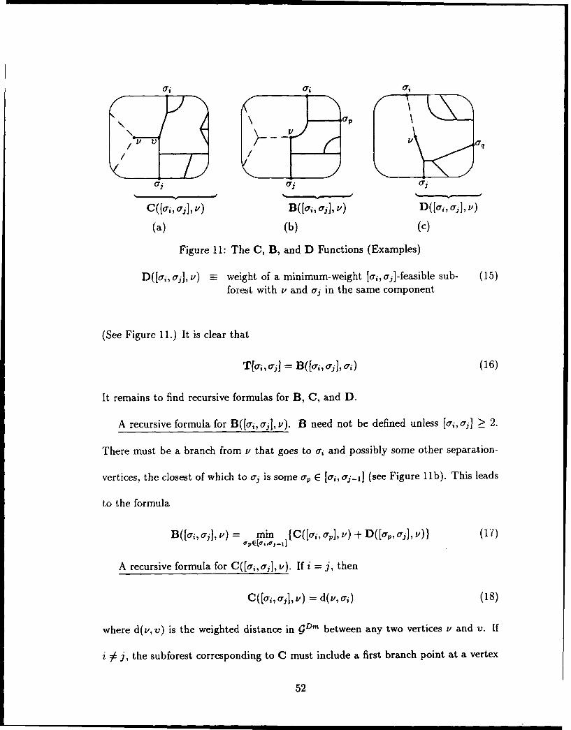
V /

aj Oaj

C([ui, 03], V) B([o,, oj], V) D([oa, oj], v)

(a) (b) (c)

Figure 11: The C, B, and D Functions (Examples)

D([a,, oj, v) - weight of a minimum-weight [ai,aj]-feasible sub- (15)forest with v and aj in the same component

(See Figure 11.) It is clear that

Tfa=, rjl-- B([oTi, oaj, oi) (16)

It remains to find recursive formulas for B, C, and D.

A recursive formula for B((oi, aj, v). B need not be defined unless [au, ,j] _! 2.

There must be a branch from v that goes to ai and possibly some other separation-

vertices, the closest of which to oj is some ap E [Oi, ao_>] (see Figure 11b). This leads

to the formula

B([a,, j, v) = min {C([ai, n], v) + D([ap, j], v)} (17)

A recursive formula for C((oa,,j], v). If i = j, then

C([a', ajI, v) = d(v, ao) (18)

where d(v, v) is the weighted distance in gDm between any two vertices v and v. If

i # j, the subforest corresponding to C must include a first branch point at a vertex

52

v and include the shortest path from v to v (see Figure lla; v may coincide with v,

ao, or oj). Thus

C([a, ajl, v) = min {d(v, v) + B([a, ai], v)} (19)"vEVDm

A recursive formula for D([ca, I], v). The tree that includes v and Oj must also

include a separation-vertex 0q E [ai+1, oj that is farthest from aj (see Figure lic).

Thus

D([a,, aj1, v) = ruin,{S([ai, Uq], t) + C([aq, aC]j, v)} (20)aqE(U,+I 6'jl

With these functions defined, we can write the following algorithm.

53

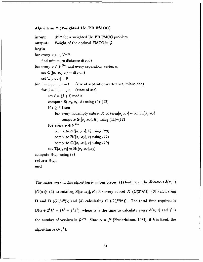
Algorithm 2 (Weighted Ue-PB FMCC)

input: GDm for a weighted Ue-PB FMCC problem

output: Weight of the optimal FMCC in

begin

for every v, v E VDm

find minimum distance d(v, v)

for every v E VDm and every separation-vertex ai

set C([ai, ai], v) = d(ai, v)

set T[ai, ail = 0for i = 1, ... , z - 1 (size of separation-vertex set, minus one)

for j = 1, ... , z (start of set)

set f= (j +i)modz

compute S([aj, at], ) using (9)-(12)

if i > 3 then

for every nonempty subset K of term[oa, all - comm[Oj, al]

compute S([aj,at], K) using (11)-(12)

for every v E VDm

compute D((j, at], v) using (20)

compute B([ac,at], v) using (17)

compute C([oa, all, v) using (19)

set T[j, a,] -= B([aj,at], aj)

compute Wopt using (8)

return Wopt

end

The major work in this algorithm is in four places: (1) finding all the distances d(v, v)

(O(a)); (2) calculating S([ai, ail, K) for every subset K (O(2kk')); (3) calculating

D and B (O(fk3 )); and (4) calculating C (O(f 2k2 )). The total time required is

O(a + 2kk4 + fkV + f 2 k2), where a is the time to calculate every d(v, v) and f is

the number of vertices in G'. Since a = f 2 [Frederickson, 1987], if k is fixed, the

algorithm is O(f 2).

54

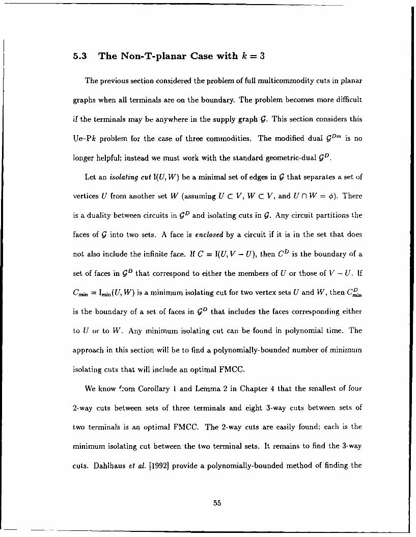
5.3 The Non-T-planar Case with k = 3

The previous section considered the problem of full multicommodity cuts in planar

graphs when all terminals are on the boundary. The problem becomes more difficult

if the terminals may be anywhere in the supply graph g. This section considers this

Ue-Pk problem for the case of three commodities. The modified dual gDm is no

longer helpful; instead we must work with the standard geometric-dual gD.

Let an isolating cut I(U, W) be a minimal set of edges in ! that separates a set of

vertices U from another set W (assuming U C V, W C V, and U n f = 0). There

is a duality between circuits in GD and isolating cuts in g9. Any circuit partitions the

faces of g into two sets. A face is enclosed by a circuit if it is in the set that does

not also include the infinite face. If C = I(U, V - U), then CD is the boundary of a

set of faces in gD that correspond to either the members of U or those of V - U. If

Cn,, = Imin(U, W) is a minimum isolating cut for two vertex sets U and W, then CL.

is the boundary of a set of faces in gD that includes the faces corresponding either

to U or to W. Any minimum isolating cut can be found in polynomial time. The

approach in this section will be to find a polynomially-bounded number of minimum

isolating cuts that will include an optimal FMCC.

We know ý-:om Corollary 1 and Lernma 2 in Chapter 4 that the smallest of four

2-way cuts between sets of three terminals and eight 3-way cuts between sets of

two terminals is an optimal FMCC. The 2-way cuts are easily found; each is the

minimum isolating cut between the two terminal sets. It remains to find the 3-way

cuts. Dahlhaus et al. [1992] provide a polynomially-bounded method of finding the

55

minimum 3-way cut separating three single vertices in a planar graph. However, in

this FMCC problem the graph will not necessarily be planar after the two terminals

in a set are linked. A modification of their method is needed.

From Proposition 2 in Chapter 4, we know that a minimum FMCC will separate

! into no more than four components. In fact, the following proposition will show

that we need only consider cuts that separate g into three or fewer components.

Two components of 9 - C = 1Z are adjacent if C contains an edge connecting them.

Two adjacent components must share a commodity (i.e. each contain one of the

commodity's terminals) if C is minimal.

Proposition 8 If an optimal three-commodity edge-cut C separates g into four com-

ponents, then C is either (1) an isolating cut, or (2) the union of two isolating cuts

separating two of the terminals from the other four.

Proof: Let C be an optimal Ue-P3 FMCC that separates ! into four components

1,1Z2,,1Z3 , 1Z4. One component must have exactly one terminal; without loss of

generality let R 1 contain sl. TR1 can only be adjacent to one other component, namely

the one containing t1, for otherwise the cut edges between it and any other component

would be superfluous. Let R2 contain t1 . Since g is connected, 1Z2 must be adjacent

to another component and share a commodity with it; let it be R3 ard suppose

s2 E 1Z2 and t2 E 1Z3 . At this point there are two possibilities: R4 can be adjacent

to either RZ2 or 1Z3; in either case we can suppose t3 E 1Z4. So the configuration

of 1Z must be like either (a) or (b) in Figure 12. In each case, C is a combination

of disjoint cuts, each of which is a minimum cut between two sets of terminals. In

56

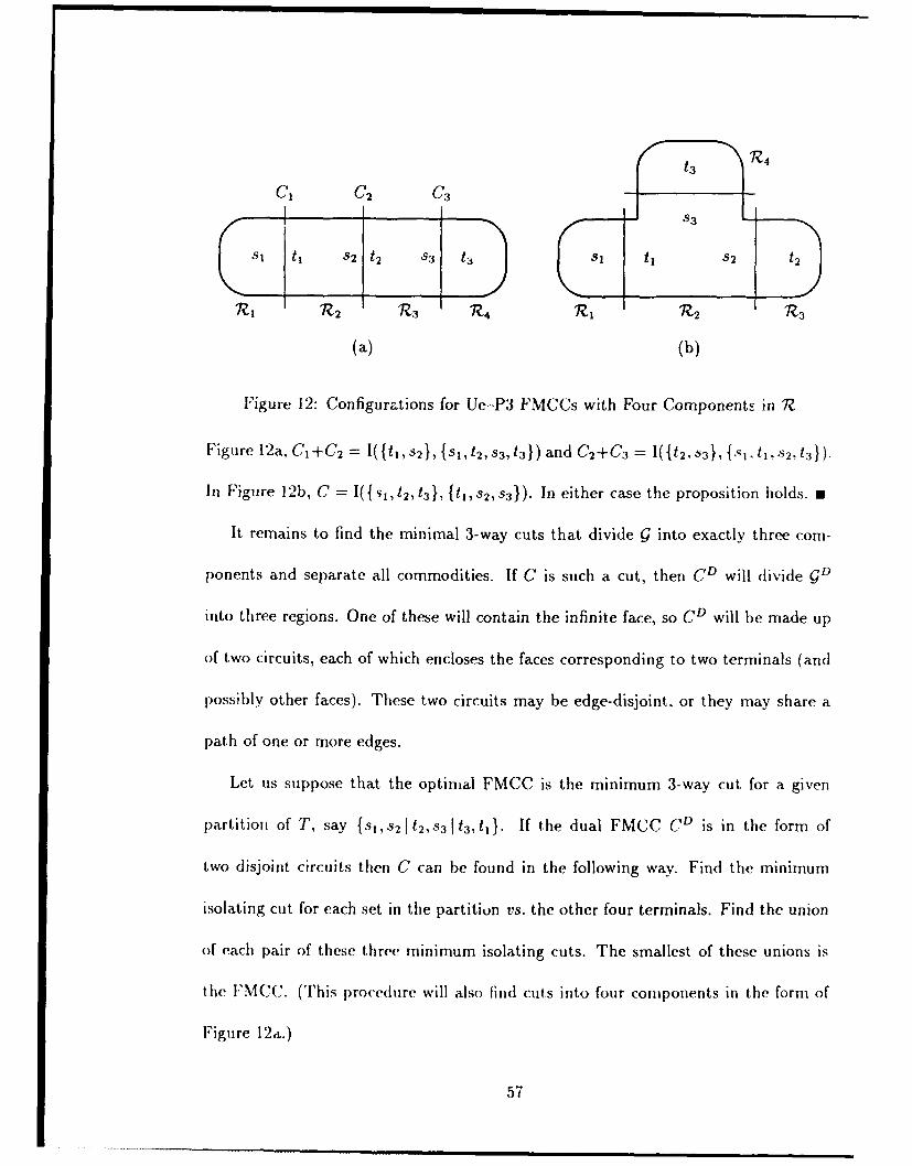
C l C 2 C 3

S tZ 4

*i t, S2 t2 S3 t3 tS2t

1z 1 12 Z3 1Z4 R1 1 32 13

(a) (b)

Figure 12: Configurations for Ue-P3 FMCCs with Four Components in 1?

Figure 12a, C-+C2 = l({tlS 2}, {sI,t 2 ,s 3 ,6t}) and C 2 +C 3 = I({t 2 ,S 3}, {.i, i,8s 2 ,t 3 }).

In Figure 12b, C = I({ 51,12, t3 }, {tI,s2,s3}). In either case the proposition holds. s

It remains to find the minimal 3-way cuts that divide g into exactly three com-

ponents and separate all commodities. If C is such a cut, then CD will divide g'

into three regions. One of these will contain the infinite face, so CD will be made up

of two circuits, each of which encloses the faces corresponding to two terminals (and

possibly other faces). These two circuits may be edge-disjoint, or they may share a

path of one or more edges.

Let us suppose that the optimal FMCC is the minimum 3-way cut for a given

partition of T, say {s, s2 It2,S31 ta, t1}. If the dual FMCC CD is in the form of

two disjoint circuits then C can be found in the following way. Find the minimum

isolating cut for each set in the partition vs. the other four terminals. Find the union

of each pair of these three minimum isolating cuts. The smallest of these unions is

the FMCC. (This procedure will also find cuts into four components in the form of

Figure 12a.)

57

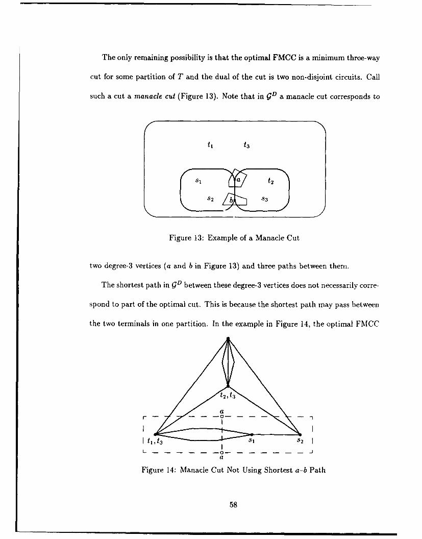
The only remaining possibility is that the optimal FMCC is a minimum three-way

cut for some partition of T and the dual of the cut is two non-disjoint circuits. Call

such a cut a manacle cut (Figure 13). Note that in QD a manacle cut corresponds to

tl t3

8S2 Ub S3

Figure 13: Example of a Manacle Cut

two degree-3 vertices (a and b in Figure 13) and three paths between them.

The shortest path in GD between these degree-3 vertices does not necessarily corre-

spond to part of the optimal cut. This is because the shortest path may pass between

the two terminals in one partition. In the example in Figure 14, the optimal FMCC

aItJ,t3 • lS2

L Oa

Figure 14: Manacle Cut Not Using Shortest a-b Path

58

when all edges are equally weighted is the six-edge manacle cut shown. However, the

shortest path between vertices a and b is the single edge corresponding to sis2.

Let f bý the number of faces in g, i.e. thc number of vertices in gD. There are

0(f2) possible choices for a and b, and if we examine all of them we are sure to find

the best manacle cut (assuming we are starting with the correct 3-partition of T and

selection of which two sets are enclosed in the manacle).

Let T1 and T2 be the sets of terminals enclosed in the manacle, let T3 be the

remaining pair, and let a and 6 be the faces of ! corresponding to the branch points.

Note that for a minimal manacle one set of consecutive vertices around the boundary

of a must fall outside the manacle, while the rest fall inside (in either of the two

interior regions). Let us call these two sets Out(a) and In(a) , and let Out(b) and

In(b) be defined the same way. If d is the maximum degree of a vertex in 0D, then

there are 0(d2) ways Out(a) can be chosen and 0(d 4 ) ways all four Out and In sets

can be selected.

The boundary of an optimal manacle corresponds to the minimum isolating cut

Imjn( T, U T2 U In(a) U In(b), T3 U Out(a) U Out(b) ). If that isolating cut does not

correspond to a simple circuit in gD, then the manacle cut is not optimal for this

selection of a, b, and their In and Out sets. Once the boundary CB of the manacle

cut is found in this way, then the remaining a-b cut is simply Imi,(TI, T2) in j - CB.

The foregoing arguments prove the correctness of the following algorithm.

59

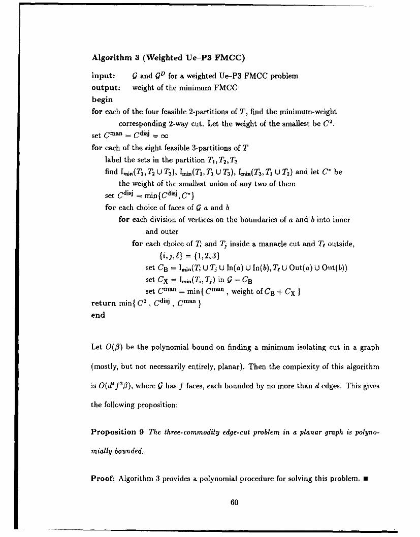
Algorithm 3 (Weighted Ue-P3 FMCC)

input: g and gD for a weighted Ue-P3 FMCC problem

output: weight of the minimum FMCC

begin

for each of the four feasible 2-partitions of T, find the minimum-weight

corresponding 2-way cut. Let the weight of the smallest be C2 .

set Cman = Cdisj = o-

for each of the eight feasible 3-partitions of T

label the sets in the partition T1, T2, T3

find Imin(T 1, T 2 U T3), Imin(T2, T, U T3 ), I.n(T3, 1 U T 2) and let C* be

the weight of the smallest union of any two of them

set Cdisj - min{Cdisi, C-}

for each choice of faces of g a and b

for each division of vertices on the boundaries of a and b into inner

and outer

for each choice of Tj and Tj inside a manacle cut and Tt outside,

{i,j,e} = {1,2,3}

set CB = Imni(Ti U Ti U In(a) U In(b), Te U Out(a) U Out(b))

set CX = Im.,(T;, Tj) in g - CB

set Cman = min{ Cman , weight of CB + CX }

return min{ C 2 , Cdisj , Cman}

end

Let 0(13) be the polynomial bound on finding a minimum isolating cut in a graph

(mostly, but not necessarily entirely, planar). Then the complexity of this algorithm

is 0(d 4f 2,3), where g has f faces, each bounded by no more than d edges. This gives

the following proposition:

Proposition 9 The three-commodity edge-cut problem in a planar graph is polyno-

mially bounded.

Proof: Algorithm 3 provides a polynomial procedure for solving this problem. n

60

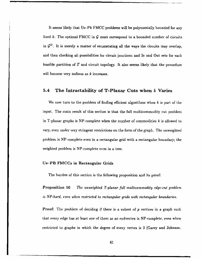
It seems likely that Ue-Pk FMCC problems will be polynomially bounded for any

fixed k. The optimal FMCC in g must correspond to a bounded number of circuits

in gD. It is merely a matter of enumerating all the ways the circuits may overlap,

and then checking all possibilities for circuit junctions and In and Out sets for each

feasible partition of T and circuit topology. It also seems likely that the procedure

will become very tedious as k increases.

5.4 The Intractability of T-Planar Cuts when k Varies

We now turn to the problem of finding efficient algorithms when k is part of the

input. The main result of this section is that the full multicommodity cut problem

in T-planar graphs is NP-complete when the number of commodities k is allowed to

vary, even under very stringent restrictions on the form of the graph. The unweighted

problem is NP-complete even in a rectangular grid with a rectangular boundary; the

weighted problem is NP-complete even in a tree.

Ue-PB FMCCs in Rectangular Grids

The burden of this section is the following proposition and its proof:

Proposition 10 The unweighted T-planar full multicommodity edge-cut problem

is NP-hard, even when restricted to rectangular grids with rectangular boundaries.

Proof: The problem of deciding if there is a subset of p vertices in a graph such

that every edge has at least one of them as an endvertex is NP-complete, even when

restricted to graphs in which the degree of every vertex is 3 [Garey and Johnson,

61

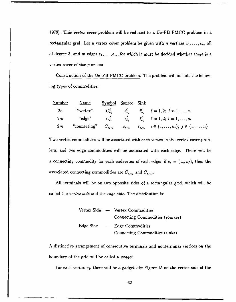
1979]. This vertex cover problem will be reduced to a Ue-PB FMCC problem in a

rectangular grid. Let a vertex cover problem be given with n vertices vl,... , vn, all

of degree 3, and m edges el,.. . e,,,, for which it must be decided whether there is a

vertex cover of size p or less.

Construction of the Ue--PB FMCC problem. The problem will include the follow-

ing types of commodities:

Number Name Symbol Source Sink

2n "vertex" Ct et t 11,2;j=1,.V., V3, Vi = 1, ;j , . ,

2m "edge" se=, ; i =1... .. , m

2m "connecting" Ge,,s, ev2 t¢,i, i E {1, ... , m}; i E {1,... ,n}

Two vertex commodities will be associated with each vertex in the vertex cover prob-

lem, and two edge commodities will be associated with each edge. There will be

a connecting commodity for each endvertex of each edge: if ej = (va, vf), then the

associated connecting commodities are Ce,,•, and Ce5,,1 .

All terminals will be on two opposite sides of a rectangular grid, which will be

called the vertex side and the edge side. The distribution is:

Vertex Side - Vertex Commodities

Connecting Commodities (sources)

Edge Side - Edge Commodities

Conncfting Commodities (sinks)

A distinctive arrangement of consecutive terminals and nonterminal vertices on the

boundary of the grid will be called a gadget.

For each vertex vj, there will be a gadget like Figure 15 on the vertex side of the

62

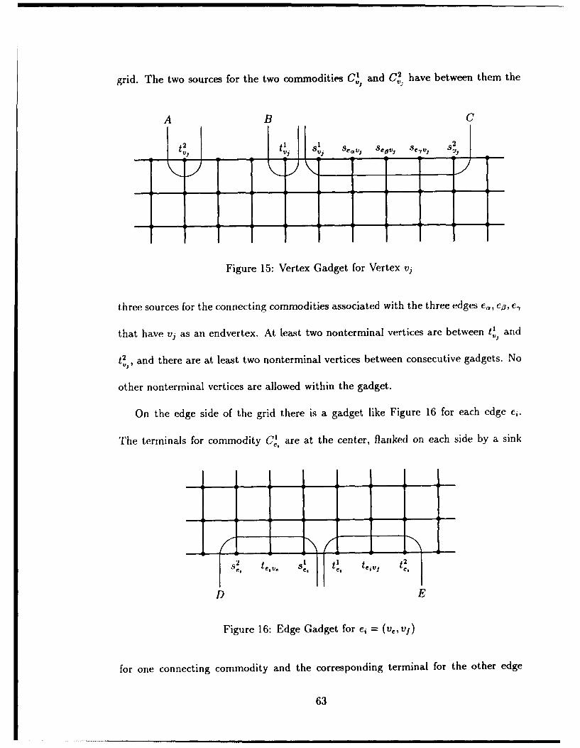
grid. The two sources for the two commodities CX and C' have between them the

A B C

P 1 sed I , S '.' e 2V, V" V Veovi seJ

Figure 15: Vertex Gadget for Vertex vj

three sources for the connecting commodities associated with the three edges eC, e', e,

that have v, as an endvertex. At least two nonterminal vertices are between t' and

tV2

V2, and there are at least two nonterminal vertices between consecutive gadgets. No

other nonterminal vertices are allowed within the gadget.

On the edge side of the grid there is a gadget like Figure 16 for each edge e1.

The terminals for commodity CI, are at the center, flanked on each side by a sink

s2 1•• I tI t,1 t

D E

Figure 16: Edge Gadget for ej = (v,, vf )

for one connecting commodity and the corresponding terminal for the other edge

63

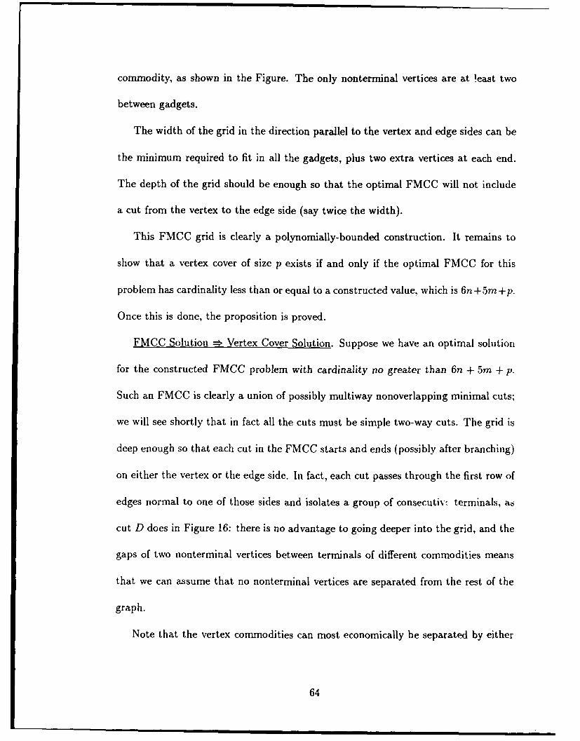
commodity, as shown in the Figure. The only nonterminal vertices are at least two

between gadgets.

The width of the grid in the direction parallel to the vertex and edge sides can be

the minimum required to fit in all the gadgets, plus two extra vertices at each end.

The depth of the grid should be enough so that the optimal FMCC will not include

a cut from the vertex to the edge side (say twice the width).

This FMCC grid is clearly a polynomially-bounded construction. It remains to

show that a vertex cover of size p exists if and only if the optimal FMCC for this

problem has cardinality less than or equal to a constructed value, which is 6n +5rm +p.

Once this is done, the proposition is proved.

FMCC Solution =' Vertex Cover Solution. Suppose we have an optimal solution

for the constructed FMCC problem with cardinality no greater than 6n + 5m + p.

Such an FMCC is clearly a union of possibly multiway nonoverlapping minimal cuts;

we will see shortly that in fact all the cuts must be simple two-way cuts. The grid is

deep enough so that each cut in the FMCC starts and ends (possibly after branching)

on either the vertex or the edge side. In fact, each cut passes through the first row of

edges normal to one of those sides and isolates a group of consecutivw terminals, as

cut D does in Figure 16: there is no advantage to going deeper into the grid, and the

gaps of two nonterminal vertices between terminals of different commodities means

that we can assume that no nonterminal vertices are separated from the rest of the

graph.

Note that the vertex commodities can most economically be separated by either

64

two cuts of three edges each isolating the sinks (A and B in Figure 15) or by one

cut of seven edges that isolates the sources and also the sources for the associated

connecting commodities (C in Figure 15). If in any vertex gadget the given optimal

FMCC cuts off one connecting commodity source without cutting off all three, it must

use at least seven edges to do so. Replace those edges with a seven-edge-cut around

the vertex commodity sources (as C), which will separate the same commodities. If

in any vertex gadget the given optimal FMCC separates no connecting commodities,

then it must use six edges; replace them if necessary with cuts isolating the vertex

commodity sinks (as A and B).

In each edge gadget, the given optimal FMCC must separate each edge commodity

with a five-edge cut (like D or E in Figure 16) that also cuts off the sink for one

associated connecting commodity. The other connecting commodity sink cannot be

isolated by fewer than three edges. Therefore the optimal FMCC must separate that

connecting commodity at a cost of at most one additional edge by putting the cut

for the corresponding vertex commodity on the sink side (like C in Figure 15), thus

cutting off the connecting commodity's source.

Now we will show that a vertex cover of size p or less can be found by taking

those vertices whose corresponding vertex commodities are separated by a cut on the

source side (like C in Figure 15). There are 6n + 5m edges known to be in the FMCC

so far: 6n for vertex commodity cuts (exclusive of extra edges for source-side cuts)

and 5m for edge commodity cuts. The remaining p or fewer edges in the FMCC must

suffice to separate the connecting commodities. This is most economically done by

65

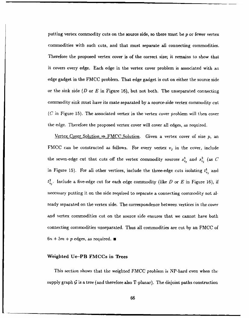
putting vertex commodity cuts on the source side, so there must be p or fewer vertex

commodities with such cuts, and that must separate all connecting commodities.

Therefore the proposed vertex cover is of the correct size; it remains to show that

it covers every edge. Each edge in the vertex cover problem is associated with an

edge gadget in the FMCC problem. That edge gadget is cut on either the source side

or the sink side (D or E in Figure 16), but not both. The unseparated connecting

commodity sink must have its mate separated by a source-side vertex commodity cut

(C in Figure 15). The associated vertex in the vertex cover problem will then cover

the edge. Therefore the proposed vertex cover will cover all edges, as required.

Vertex Cover Solution =€, FMCC Solution. Given a vertex cover of size p, an

FMCC can be constructed as follows. For every vertex vj in the cover, include

the seven-edge cut that cuts off the vertex commodity sources s' and s' (as C

in Figure 15). For all other vertices, include the three-edge cuts isolating t', and

t2 Include a five-edge cut for each edge commodity (like D or E in Figure 16), ifVI.

necessary putting it on the side required to separate a connecting commodity not al-

ready separated on the vertex side. The correspondence between vertices in the cover

and vertex commodities cut on the source side ensures that we cannot have both

connecting commodities unseparated. Thus all commodities are cut by an FMCC of

6n + 5m + p edges, as required. a

Weighted Ue-PB FMCCs in Trees

This section shows that the weighted FMCC problem is NP-hard even when the

supply graph ! is a tree (and therefore also T-planar). The disjoint paths construction

66

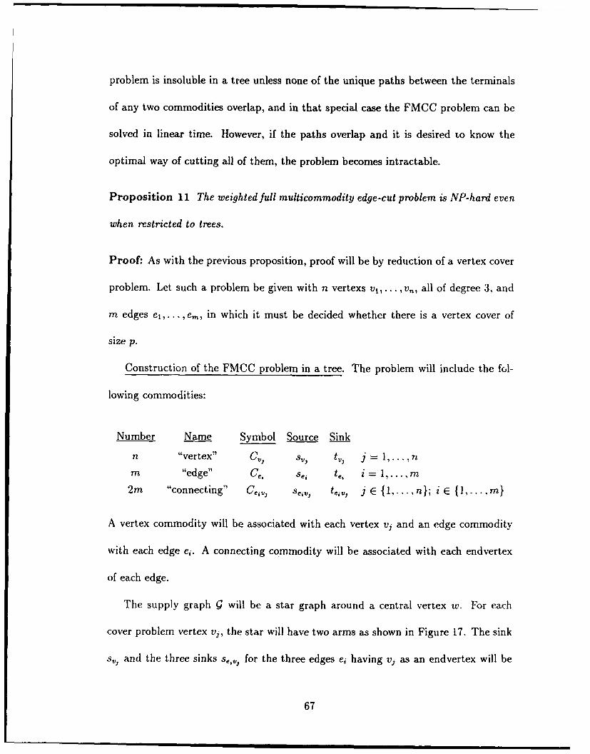
problem is insoluble in a tree unless none of the unique paths between the terminals

of any two commodities overlap, and in that special case the FMCC problem can be

solved in linear time. However, if the paths overlap and it is desired to know the

optimal way of cutting all of them, the problem becomes intractable.

Proposition 11 The weighted full multicommodity edge-cut problem is NP-hard even

when restricted to trees.

Proof: As with the previous proposition, proof will be by reduction of a vertex cover

problem. Let such a problem be given with n vertexs vj,. .. , v,,, all of degree 3, and

m edges el,. ... , em, in which it must be decided whether there is a vertex cover of

size p.

Construction of the FMCC problem in a tree. The problem will include the fol-

lowing commodities:

Number Name Symbol Source Sink

n "vertex" C", s', t,, j = 1 nm "edge" C., se te i = 1, ... m

2m "connecting" Co, s5 eiv, tev,, j E {1, ... n}; i E {1,...,m}

A vertex commodity will be associated with each vertex vi and an edge commodity

with each edge e;. A connecting commodity will be associated with each endvertex

of each edge.

The supply graph Q will be a star graph around a central vertex w. For each

cover problem vertex vj, the star will have two arms as shown in Figure 17. The sink

s,, and the three sinks s,,,, for the three edges e; having vi as an endvertex will be

67

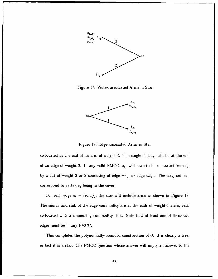
'Se'ev. SIV,8 ej 3

2

Figure 17: Vertex-associated Arms in Star

Sc'

1

teivy

Figure 18: Edge-associated Arms in Star

co-located at the end of an arm of weight 3. The single sink t• will be at the end

of an edge of weight 2. In any valid FMCC, s., will have to be separated from tv,

by a cut of weight 3 or 2 consisting of edge ws.2 or edge wtv,. The ws•, cut will

correspond to vertex vj being in the cover.

For each edge e, = (ve, vf), the star will include arms as shown in Figure 18.

The source and sink of the edge commodity are at the ends of weight-1 arms, each

co-located with a connecting commodity sink. Note that at least one of these two

edges must be in any FMCC.

This completes the polynomially-bounded construction of g. It is clearly a tree;

in fact it is a star. The FMCC question whose answer will imply an answer to the

68

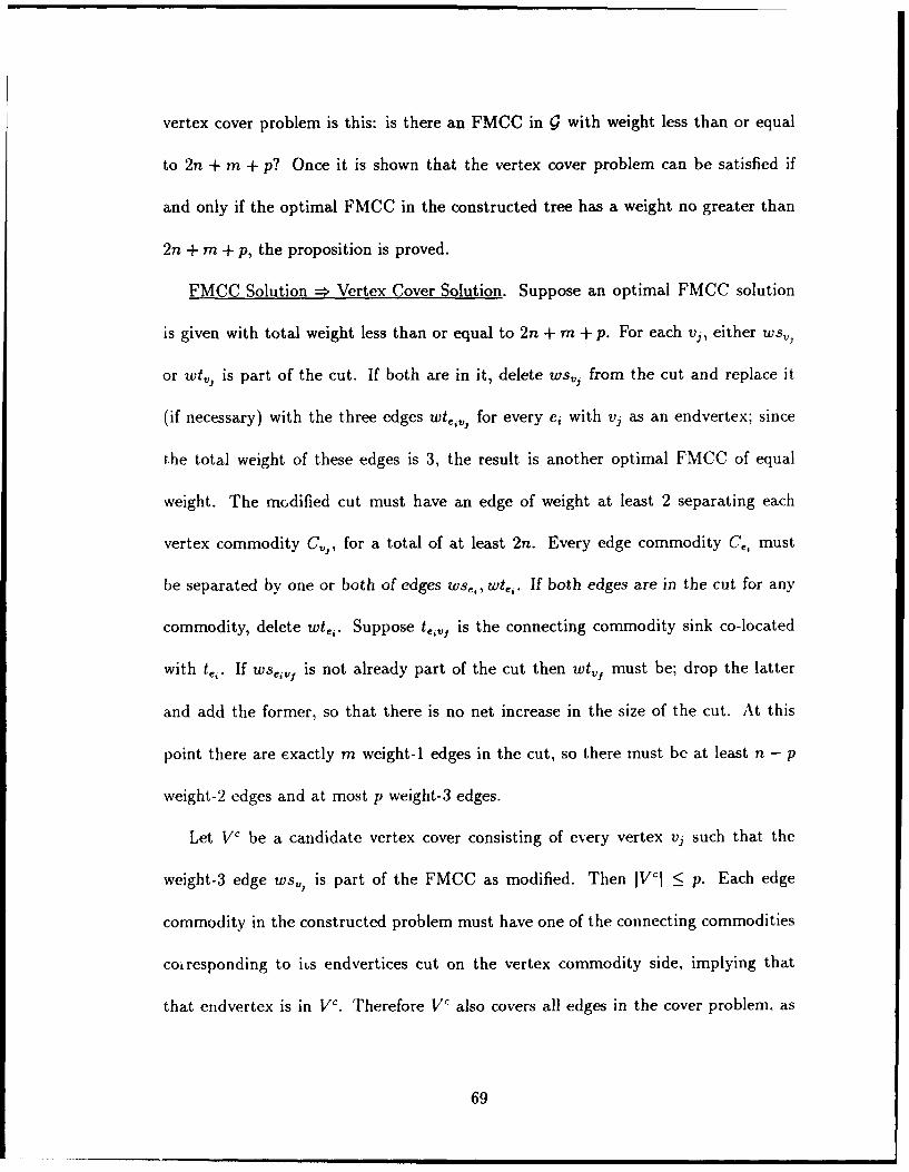
vertex cover problem is this: is there an FMCC in g with weight less than or equal

to 2n + m + p? Once it is shown that the vertex cover problem can be satisfied if

and only if the optimal FMCC in the constructed tree has a weight no greater than

2n + m + p, the proposition is proved.

FMCC Solution =:. Vertex Cover Solution. Suppose an optimal FMCC solution

is given with total weight less than or equal to 2n + m + p. For each vj, either ws,1

or wt,,1 is part of the cut. If both are in it, delete wst,, from the cut and replace it

(if necessary) with the three edges wt,,,,, for every ej with vj as an endvertex; since

the total weight of these edges is 3, the result is another optimal FMCC of equal

weight. The mcdified cut must have an edge of weight at least 2 separating each

vertex commodity Ci,,, for a total of at least 2n. Every edge commodity Ce, must

be separated by one or both of edges wse,, wte,. If both edges are in the cut for any

commodity, delete wt,,. Suppose t•,,, is the connecting commodity sink co-located

with te,. If ws,,,1 is not already part of the cut then wt,,, must be; drop the latter

and add the former, so that there is no net increase in the size of the cut. At this

point there are exactly m weight-1 edges in the cut, so there must be at least n - p

weight-2 edges and at most p weight-3 edges.

Let VC be a candidate vertex cover consisting of every vertex vj such that the

weigbt-3 edge ws., is part of the FMCC as modified. Then IVci < p. Each edge

commodity in the constructed problem must have one of the connecting commodities

coiresponding to its endvertices cut on the vertex commodity side, implying that

that endvertex is in VC. Therefore V' also covers all edges in the cover problem, as

69

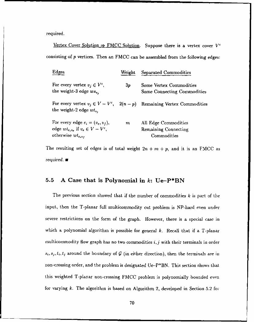
required.

Vertex Cover Solution •:ý FMCC Solution. Suppose there is a vertex cover Vc

consisting of p vertices. Then an FMCC can be assembled from the following edges:

Edges Weight Separated Commodities

For every vertex vi E Vc, 3p Some Vertex Commoditiesthe weight-3 edge ws,,, Some Connecting Commodities

For every vertex vj E V - Vc, 2(n - p) Remaining Vertex Commoditiesthe weight-2 edge wtv)

For every edge e, = (ve, vf), m All Edge Commodities

edge wtc,,e if ve E V - Vc, Remaining Connectingotherwise wt•,,q Commodities

The resulting set of edges is of total weight 2n + m + p, and it is an FMCC as

required. n

5.5 A Case that is Polynomial in k: Ue-P*BN

The previous section showed that if the number of commodities k is part of the

input, then the T-planar full multicommodity cut problem is NP-hard even under

severe restrictions on the form of the graph. However, there is a special case in

which a polynomial algorithm is possible for general k. Recall that if a T-planar

multicommodity flow graph has no two commodities ij with their terminals in order

si, sj, ti, tj around the boundary of G (in either direction), then the terminals are in

non-crossing order, and the problem is designated Ue-P*BN. This section shows that

this weighted T-planar non-crossing FMCC problem is polynomially bounded even

for varying k. The algorithm is based on Algorithm 2, developed in Section 5.2 for

70

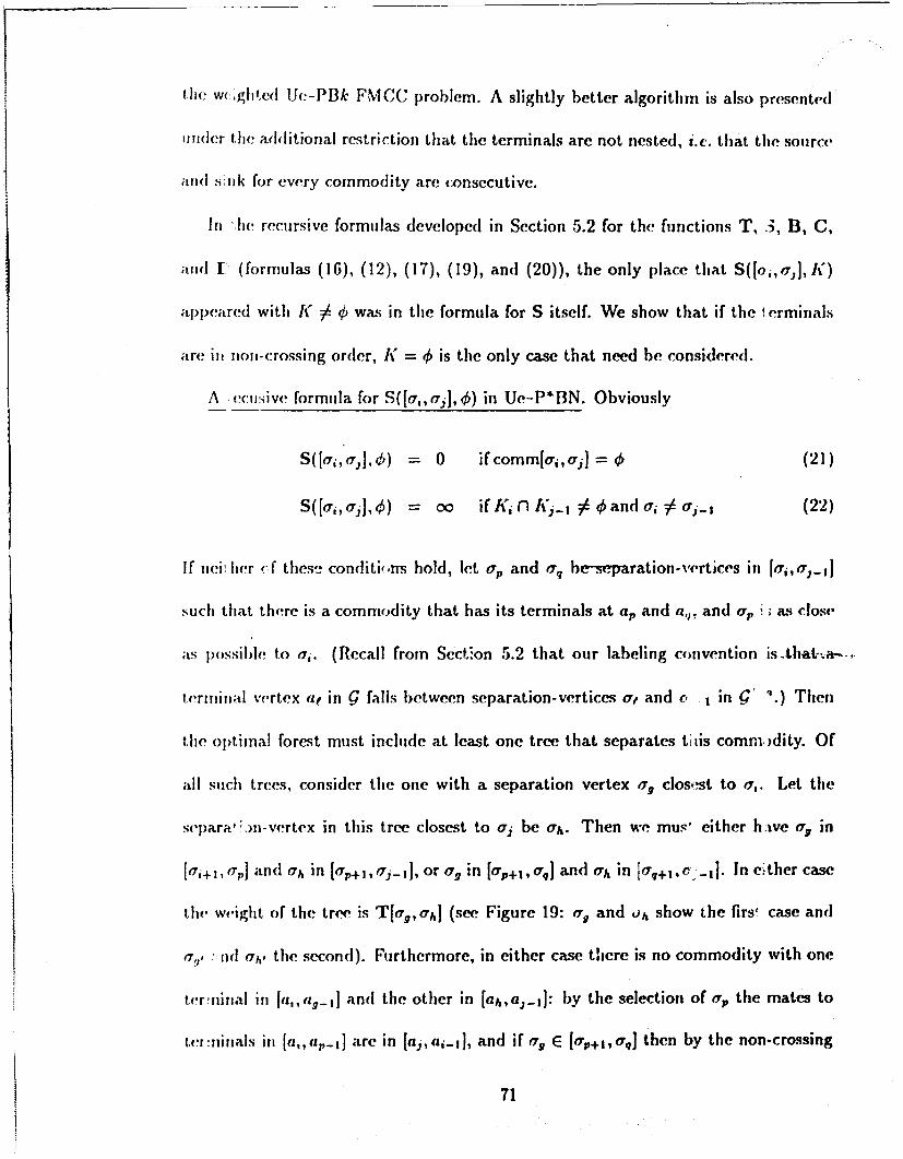
the wc-ghted Ue-PBk FMCC problem. A slightly better algorithm is also presented

,11ider the additional restriction that the terminals are not nested, i.c. that tile source

antd -ink for every commodity are consecutive.

In ý he recursive formulas developed in Section 5.2 for the functions T, 3, B, C,

and I (formulas (16), (12), (17), (19), and (20)), the only place that S([o,, j], K)

appeareld with K $ was in the formula for S itself. We show that if the ! erminals

are in non-crossing order, K = ) is the only case that need be considered.

A ccus:ive formula for S{[',, aj], 0) in Ue-P*BN. Obviously

S([•,,•,I,•) = 0 ifcomm[uja,aj]= (21)

S([aj,,aj],) = oo ifKilnKp.,$.k4andj6a,=o._, (22)

If Tei: her (-f these conditi.n-s hold, let ap and taq be-separation-vertices in [(7i, t7,-]

Such that there is a commodity that has its terminals at ap and a,,, and q, i; as close

;as possible to eoj. (Recall from Section 5.2 that our labeling convention is-that-a-

terminal vertex at in g falls between separation-vertices at and c , in !" '.) Then

the optimal forest must include at least one tree that separates tiis commndity. Of

all such trees, consider the one with a separation vertex a, closest to oa,. Let the

separa,;')n-vertex in this tree closest to aj be oh. Then we mus' either have a. in

[a'i+vo71 and( ah in [ or o, in [o'+,,,aj and al, in [a'q+I,c. ,I. In either case

tihe weight of the tree is T[e,,a'h] (see Figure 19: a., and al show the first case and

rg, : r !y,' tihe second). Furthermore, in either case there is no commodity with one

tverninal in [a,.,-_] and the other in [ah,a,-.]: by the selection of or, the mates to

tcz:riirals i, [a,,a,-,_] are in [a,,a,_,], and if a'g E [a'p+jOqj then by the non-crossing

71

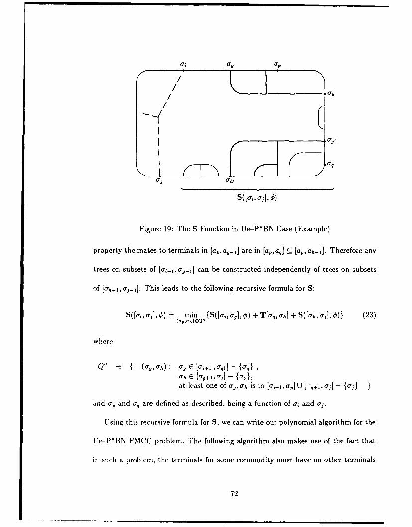
aiag ap

/ h/

019

I 0

Odhj

s([o•, ai], 0)

Figure 19: The S Function in Ue-P*BN Case (Example)

property the mates to terminals in [ap, a•,,1 are in [ap, aq] 9 ap, ahl]. Therefore any

trees on subsets of , ag-] can be constructed independently of trees on subsets

of [Ch+1, aj- ]. This leads to the following recursive formula for S:

S([a,, ai], ) = min ,,{S([aj, ,], 0) + T[a,, ahl] + S([ah, ai], 0)} (23)(7g,Ch)EQ

where

Q" - { (ag, h): ag E [0+i + ,ql - } I,ah E [l+a,, aj- {faj ,at least one of ay,ah is in [ai+i,ap] U q+,, a'] - {Jai II

and ap and aq are defined as described, being a function of ai and a,.

Using this recursive formula for S, we can write our polynomial algorithm for the

Ue-P*BN FMCC problem. The following algorithm also makes use of the fact that

in such a problem, the terminals for some commodity must have no other terminals

72

between them on the boundary of g. It is to be compared with Algorithm 2 on p. 54,

which is for the general Ue-PB FMCC problem, but is not polynomial in k.

Algorithm 4 (Weighted Ue-P*BN FMCC)

input: "Dm for a weighted Ue-P*BN FMCC problem, with the separation-vertices numbered so that K1 fn K, # 0

output: Weight of the minimum forest in gDm that corresponds to the optimal

FMCC in gbeginfor every v, v E VDm

find minimum distance d(v, v)

for every v E VDm and every separation-vertex ai

set C([i,ail],v) = d(ai, v)

set To'i, ail = 0

for i= 1, ... , z - 1 (size of separation-vertex set, minus one)

forj=1,...,z (start of set)set I = (j+ i) mod z

compute S(aj, at], 0) using (21)-(23)

for every v E VD,

compute D([aj,at],v) using (20)

compute B([a.,at],,v) using (17)

compute C(fao, at],v) using (19)

set T[a, at] = B([aj,at],aj)compute Wopt = rmin {T[aal,] + S([ai, a,],o)}

i=2...z

return Wopt

end

The complexity of this algorithm is O(a + k4 + fk 3 + f 2k2), where again a is the

bound on finding all the distances d(v, v) and f is the number of vertices in gDm. It

also provides the proof for the following proposition:

Proposition 12 The weighted T-planar full multicommodity edge-cut problem is

polynomially bounded if the terminals are restricted to be in non-crossing order.

73

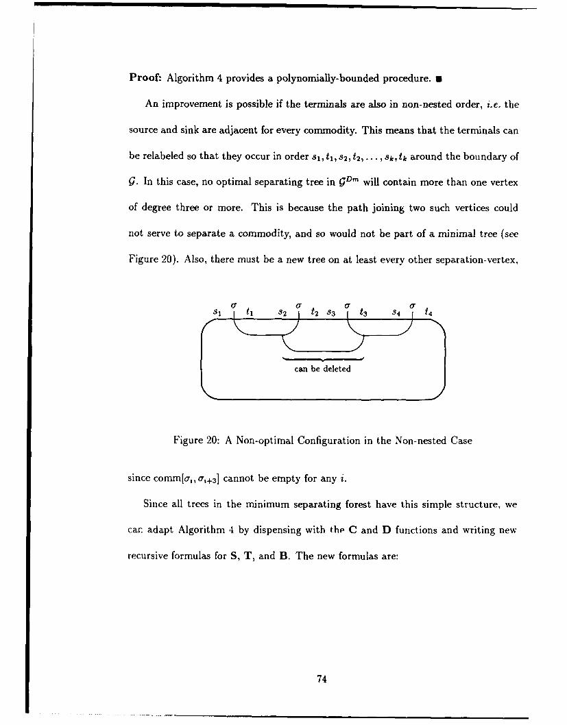
Proof: Algorithm 4 provides a polynomially-bounded procedure. 0

An improvement is possible if the terminals are also in non-nested order, i.e. the

source and sink are adjacent for every commodity. This means that the terminals can

be relabeled so that they occur in order sI, t1 , S2, t2 ,.. .- ,3I, tk around the boundary of

g. In this case, no optimal separating tree in g", will contain more than one vertex

of degree three or more. This is because the path joining two such vertices could

not serve to separate a commodity, and so would not be part of a minimal tree (see

Figure 20). Also, there must be a new tree on at least every other separation-vertex,

S1It 2It 2 S3 I13 84 N4

can be deleted

Figure 20: A Non-optimal Configuration in the Non-nested Case

since comm[ai, ai+31 cannot be empty for any i.

Since all trees in the minimum separating forest have this simple structure, we

car adapt Algorithm 4 by dispensing with the C and D functions and writing new

recursive formulas for S, T, and B. The new formulas are:

74

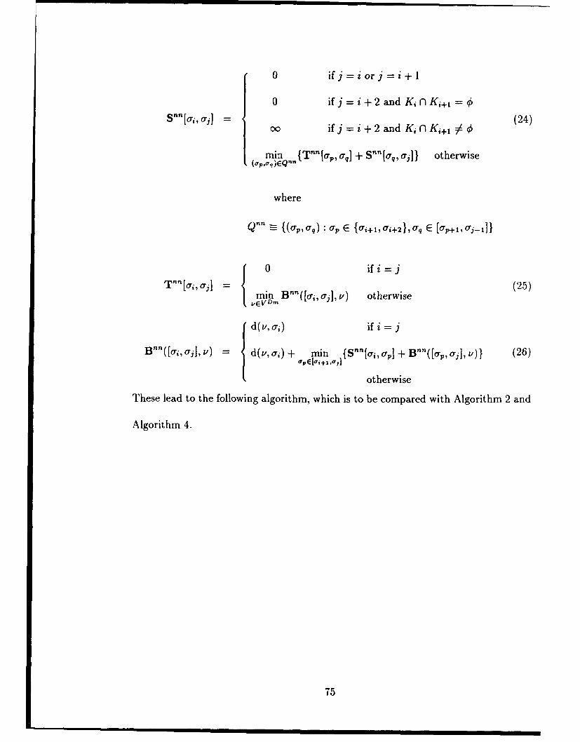
0 ifj =Z iorj = z+ 1

0 if j = i + 2 and Ki n Kji+=

00 ifj=i+2andKflKi+,l 54 (24)

min {T""[ap, aq] + Sfl n[aq, aij} otherwise(O'p,aq)EQnn-

where

Q"" =- {(pa,) {:E s+1,,i,+2},Oq E [op+j,ay-,j}

S 0 ifi2 = j

="[, {j = (25)Tmin B'n([ai,j],) V otherwiseLEVDm

f d(v, ai) if i= j

Bnn([O,, a,], V)= d(v, a) + min {S"'[ao,ap] + Bn([aaj],v)} (26)

otherwise

These lead to the following algorithm, which is to be compared with Algorithm 2 and

Algorithm 4.

75

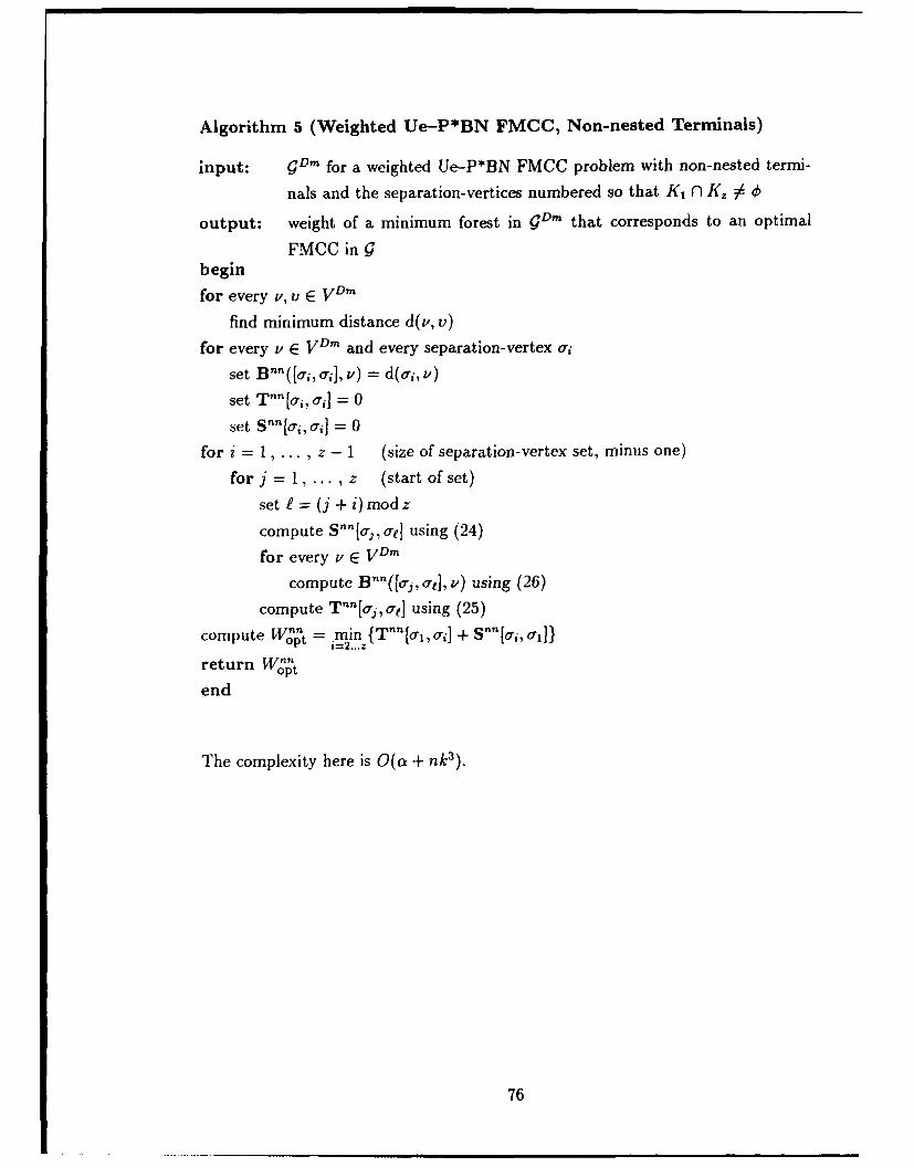
Algorithm 5 (Weighted Ue-P*BN FMCC, Non-nested Terminals)

input: gDm for a weighted Ue--P*BN FMCC problem with non-nested termi-

nals and the separation-vertices numbered so that K, n K,, $-

output: weight of a minimum forest in GDm that corresponds to an optimal

FMCC inbegin

for every v, v E VDm

find minimum distance d(v, v)

for every v E VD- and every separation-vertex a,

set Bn'([o',,oa,], v) = d(au, v)

set Tn1[o'i, o''] = 0

set S •[0, cri] = 0

for i = 1, ... , z - 1 (size of separation-vertex set, minus one)

forj=l,...,z (start of set)set f = (j + i)modz

compute Snn[oj, ae] using (24)

for every v E VDm

compute Bnfn([foGj , .') using (26)

compute Tn"[aj,ae] using (25)compute Wof = min {Tn,[u,,io] + S""[0',o',]}

i=2 ... z

return Wor"t

end

The complexity here is O(ca + nk 3).

76

6 PARTIAL MULTICOMMODITY CUTS IN

T-PLANAR GRAPHS

This chapter examines the problem if finding partial multicommodity cuts in

T-planar graphs. Results are found and algorithms described for three special cases

when the terminals are in non-crossing order (UeEP*BN). These are the cases in

which r = k - I (Section 6.2), where r = k - 2 (Section 6.3), and where r = 1 (Sec-

tion 6.4). Unlike the previous chapter, only unweighted problems will be considered.

It was noted in Chapter 4 that a partial multicommodity cut problem cannot be

easier than the corresponding disjoint paths problem, and that consequently many

restricted PMCC problems are NP-hard (Proposition 4). Based on the results of the

last chapter (Proposition 10) we can add that the partial multicommodity cut problem

is NP-hard even when restricted to planar grids with all terminals on the boundary.

Clearly the search for good PMCC algorithms should begin with graph configurations

in which the disjoint paths problem is well-characterized. Furthermore, the charac-

teristics of the configurations should persist when edges are deleted from the graph.

This makes the many DJP results for Eulerian graphs much less useful. However,

Section 6.1 will show that the DJP problem can be characterized for the case of T-

planar graphs with the terminals in non-crossing order-the U-EP*BN case. Also.

Ue-P*BN is the most general FMCC case for which there exists a polynomial algo-

rithm (Alg. 4). Therefore we consider the class UeEP*BN for partial multicommodity

cut algorithms. The next section gives the necessary characterization of disjoint paths

in T-planar non-crossing graphs.

6.1 Disjoint Paths in Non-crossing T-Planar Graphs

The following proposition shows that in an undirected graph with all terminals

on the boundary in non-crossing order (U-EP*BN), the disjoint paths construction

problem has a solution if and only if the general cut condition (GCC; defined on p. 23)

is satisfied. This result has been noted before, but it seems that a proof has never

been published. Schrijver [n.d.] suggests proving it by reducing it to an instance of

the corresponding vertex-disjoint paths problem. What follows is a different proof.,

which uses a recently-published result by Frank (19901.

Frank showed that in a U-EP* DJP problem in which each commodity has its

terminals on one of two faces, the GCC plus an intersection criterion (IC) is necessary

and sufficient for the existence of a solution. (This result was reviewed in Chapter 3.

p. 25.) For any X C V, let s(X) be the surplus (defined on p. 24) of P(X). The IC

requires that for any two subsets X and Y of V, if s(X) = s(Y) = 0, then s(X fn Y)

must be even. We will need the following lemma to apply this result to the more

restricted U-EP*BN case.

Lemma 5 In a U-EP*BN problem, if the GCC is satisfied but the IC violated, then

the IC is violated for some vertex sets X and Y such that X fl Y, X\Y, V\(X U Y),

and Y\X all induce simple cuts, and their intersections with the boundary of g occur

78

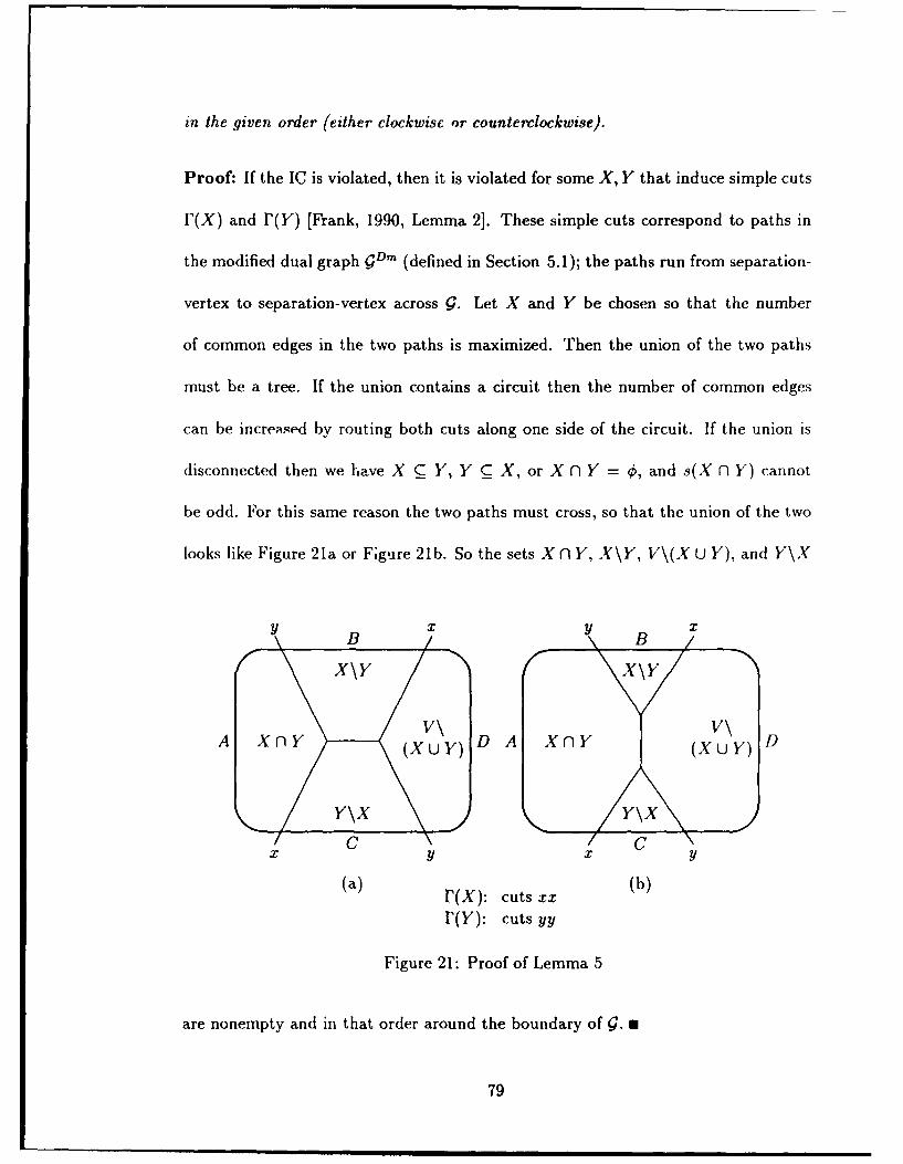
in the given order (either clockwise or counterclockwise).

Proof: If the IC is violated, then it is violated for some X, Y that induce simple cuts

[(X) and 17(Y) [Frank, 1990, Lemma 2]. These simple cuts correspond to paths in

the modified dual graph gDO (defined in Section 5.1); the paths run from separation-

vertex to separation-vertex across 9. Let X and Y be chosen so that the number

of common edges in the two paths is maximized. Then the union of the two paths

must be a tree. If the union contains a circuit then the number of common edges

can be increased by routing both cuts along one side of the circuit. If the union is

disconnected then we have X C Y, Y C X, or X n Y = 0, and s(X n Y) cannot

be odd. For this same reason the two paths must cross, so that the union of the two

looks like Figure 21a or Figure 21b. So the sets X n Y, X\Y, V\(X U Y), and Y\X

yx y/ xB B

X\Y X\Y

V\ V\A XflY (XUY) D A Xn (X UY) D

Y\X Y\X

C C

(a) r() cuts (b)

F(Y): cuts yy

Figure 21: Proof of Lemma 5

are nonempty and in that order around the boundary of •. U

79

Proposition 13 In an edge-disjoint paths construction problem in a T-planar graph

with terminals in non-crossing order, the general cut condition is necessary and suf-

ficient for the existence of a solution.

Proof: The method is to show that if all the terminals are on exactly one face

and in non-crossing order, the GCC implies the IC. The proposition then follows

immediately from Frank's result. Suppose that the GCC is satisfied in some U-

EP*BN graph Q but the IC is violated. Then by Lemma 5 it must be violated for

some vertex sets X and Y whose induced simple cuts divide g into four parts as

described. Let A =-X nY, B = A \Y, C = Y\X, and D V\(X n Y), as in

Figure 21. Then s(A) is odd, and s(A) >_ 1. For P,Q E {A,B,C,D}, let g(P,Q) be

the number of edges in G with one endvertex in P and the other in Q, let h(P,Q)

be the number of commodities with one terminal in P and the other in Q, and let

s(P, Q) = g(P, Q) - h(P, Q).

The crucial observation is that because of planarity and the non-crossing order of

the terminals, at least one of g(A, D) and g(B, C) must be zero, and at least one of

h(A, D) and h(B, C) must be zero. From Figure 21, it is clear that in configuration

(a) there are edges of 9 between B and C and in (b) between A and D, but never

between both pairs in the same graph, giving the result for g. The non-crossin6 order

of the terminals forbids commodities being shared between A and D and between B

and C at the same time, giving the result for h. This observation gives rise to three

cases.

80

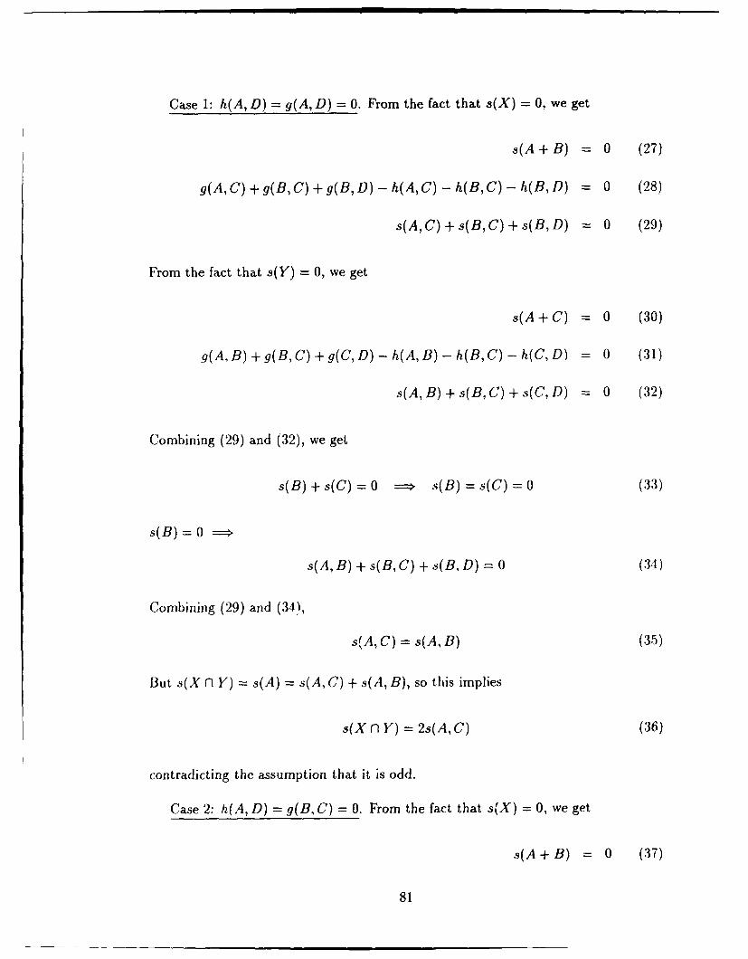
Case 1: h(A,D) = g(A,D) = 0. From the fact that s(X) = 0, we get

s(A+B) = 0 (27)

g(A, C) + g(B, C) + g(B, D) - h(A, C) - h(B, C) - h(B, D) = 0 (28)

s(A, C) + s(B, C) + s(B, D) = 0 (29)

From the fact that s(Y) = 0, we get

s(A+C) = 0 (30)

g(A,B) +g(B,C) +g(C,D) - h(A,B) - h(B,C) - h(C, D) = 0 (31)

s(A, B) + s(B, C) +s(C, D) = 0 (32)

Combining (29) and (32), we get

s(B) + s(C) = 0 ==* s(B) = s(C) = 0 (33)

s(B)=0 ==0

s(A, B) + s(B, C) + s(B, D) = 0 (34)

Combining (29) and (34),

s(A, C) = s(A, B) (35)

But s(X n Y) = s(A) = s(A, C) + s(A, B), so this implies

s(X n Y) = 2s(A, C) (36)

contradicting the assumption that it is odd.

Case 2: h(A, D) = g(B, C) = 0. From the fact that s(X) = 0, we get

s(A+B) = 0 (37)

81

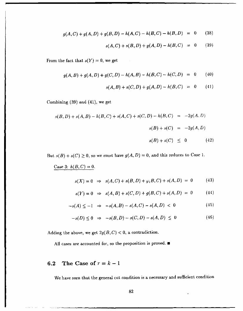
g(A,C) +g(A,D) +g(B,D) - h(A,C) - h(B,C) - h(B,D) = 0 (38)

s(A, C) + s(B, D) + g(A, D) - h(B, C) = 0 (39)

From the fact that s(Y) = 0, we get

g(A, B) + g(A, D) + g(C, D) - h(A, B) - h(B, C) - h(C, D) = 0 (40)

s(A,B)+s(C,D) +g(A,D) - h(B,C) = 0 (41)

Combining (39) and (41), we get

s(B, D) + s(A, B) - h(B, C) + s(A, C) + s(C, D) - h(B, C) = -2g(A. D)

s(B) + s(C) = -2g(A,D)

s(B) + s(C) <_ 0 (42)

But s(B) + s(C) Ž_ 0, so we must have g(A, D) = 0, and this reduces to Case 1.

Case 3: h(B, C) - 0.

s(X) =0 = s(A, C) + s(B, D) + y"B, C) + s(A, D) = 0 (43)

s(Y) =0 s(A,B)+s(C,D)+g(B,C)+s(A,D) = 0 (44)

-s(A) _ -1 • -s(A,B) - s(A,C) - s(A,D) < 0 (45)

-s(D) _ 0 =, -s(B, D) - s(C, D) - s(A, D) K 0 (46)

Adding the above, we get 2g(B, C) < 0, a contradiction.

All cases are accounted for, so the proposition is proved. 0

6.2 The Caseof r=k-1

We have seen that the general cut condition is a necessary and sufficient condition

82

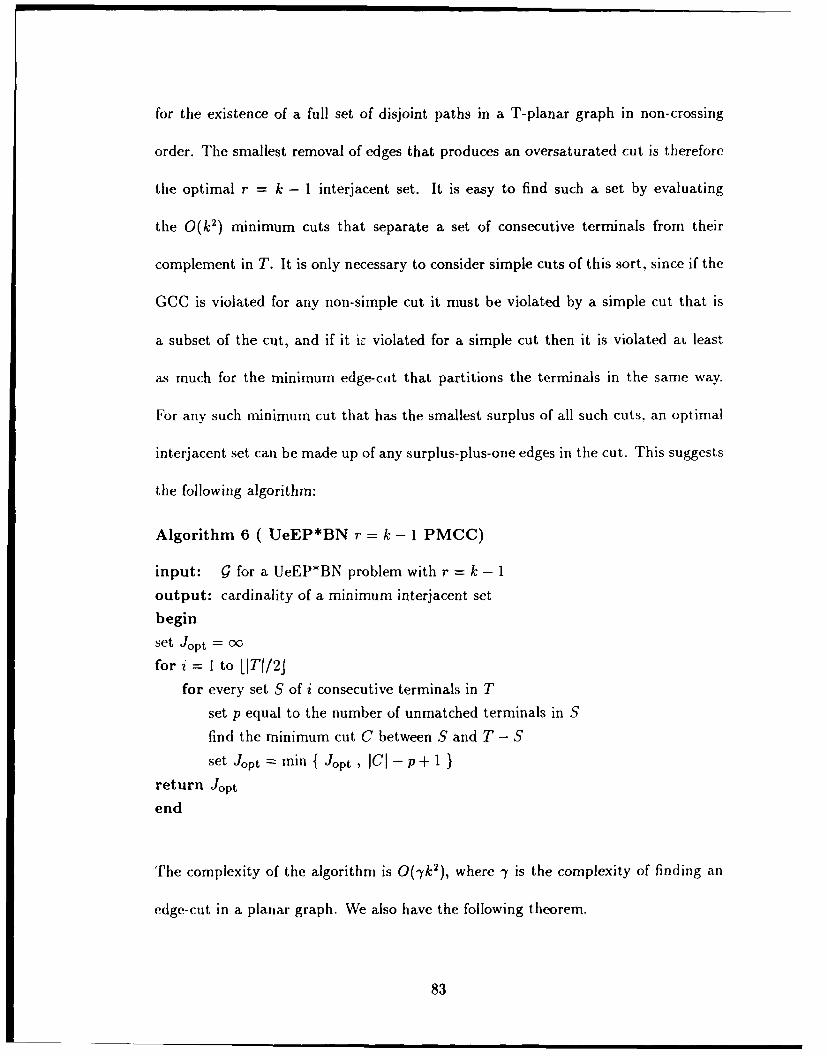
for the existence of a full set of disjoint paths in a T-planar graph in non-crossing

order. The smallest removal of edges that produces an oversaturated cut is therefore

the optimal r = k - 1 interjacent set. It is easy to find such a set by evaluating

the 0(k2 ) minimum cuts that separate a set of consecutive terminals from their

complement in T. It is only necessary to consider simple cuts of this sort, since if the

GCC is violated for any non-simple cut it must be violated by a simple cut that is

a subset of the cut, and if it iz violated for a simple cut then it is violated aL least

as much for the minimum edge-cat that partitions the terminals in the same way.

For any such minimum cut that has the smallest surplus of all such cuts, an optimal

interjacent set can be made up of any surplus-plus-one edges in the cut. This suggests

the following algorithm:

Algorithm 6 ( UeEP*BN r = k - 1 PMCC)

input: 9 for a UeEP*BN problem with r = k - 1

output: cardinality of a minimum interjacent set

begin

set Jopt = oc

for i = 1 to [IT!/2i

for every set S of i consecutive terminals in T

set p equal to the number of unmatched terminals in S

find the minimum cut C between S and T - S

set Jopt =m in { Jopt , ICI- p +1return Jopt

end

The complexity of the algorithm is 0(' 7 k2 ), where y is the complexity of finding an

edge-cut in a planar graph. We also have the following theorem.

83

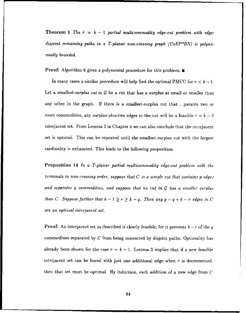
Theorem 1 The r = k - 1 partial multicommodity edge-cut problem with edge-

disjoint remaining paths in a T-planar non-crossing graph (UeEP*BN) is polyno-

mially bounded.

Proof: Algorithm 6 gives a polynomial procedure for this problem. 0

In many cases a similar procedure will help find the optimal PMCC for r < k - 1.

Let a smallest-surplus cut in g be a cut that has a surplus as small or smaller than

any other in the graph. If there is a smallest-surplus cut that . parates two or

more commodities, any surplus-plus-two edges in the cut will be a feasible r = k - 2

interjacent set. From Lemma 3 in Chapter 4 we can also conclude that the intorjacent

set is optimal. This can be repeated until the smallest-surplus cut with the largest

cardinality is exhausted. This leads to the following proposition.

Proposition 14 In a T-planar partial multicommodity edge-cut problem with the

terminals in non-crossing order, suppose that C is a simple cut that contains p edges

and separates q commodities, and suppose that no cut in g has a smaller surplus

than C. Suppose further that k -I > r > k - q. Then any p - q + k - r edges in C

are an optimal interjacent set.

Proof: An interjacent set as described is clearly feasible, for it prevents k - r of the q

commodities separated by C from being connected by disjoint paths. Optimality has

already been shown for the case r = k - 1. Lemma 3 implies that if a new feasible

interjacent set can be found with just one additional edge when r is decremented,

then that set must be optimal. By induction, each addition of a new edge from C

84

to the interjacent set results in a new optimal set for a value of r one smaller, until

every edge in C is in the set. 0

However, when r < k- I this proposition will only help us when there is a smallest-

surplus cut that separates at least k - r commodities. The general problem becomes

significantly more complicated, as we will see in the next section.

6.3 The Case of r=k-2

Let JP be an optimal interjacent set for a PMCC problem with r = k - 2 in a

graph ! in which a full set of k disjoint paths can be found. For any e E P, the set

{e} has the property that exactly k - 1 disjoint paths can be found in G - (J* - {e}).

Let J 2 be a maximum-cardinality subset of J* such that exactly k - 1 disjoint paths

can be found in G - (J* - J2). Then for any f E J - J2, a full set of k paths can be

found in G - (J* - (J 2 + {f})). Let J1 -= P - J2, so that J, and J2 are a partition of

J*. If the edges of J1 are removed from g one at a time, k disjoint paths are possible

until the last edge is removed. J1 is therefore a minimal PMCC for r = k - 1. If the

edges of J2 are then removed, k - 1 paths are possible until the removal of the last

edge of J2 (and of J*).

If we are somehow given the correct J1, we might expect it to be fairly easy to

find J 2 and complete the interjacent set. The method of finding P will be to consider

the forms that G - Ji might take. It will turn out that J2 is indeed easy to find, and

furthermore its relationship to J1 is such that J1 is also easy to find.

The disjoint paths construction problem has no solution in ! - J1, so the general

85

cut condition must be violated somewhere in it (Proposition 13). However, k - 1

paths can be drawn in Q - 3I, so it can have no cut with a surplus of -2 or less.

Therefore there are one or more smallest-surplus cuts in g - J1 with a surplus of -1.

We can consider two cases: either there is such a negative-surplus cut that contains

an edge of g - ,/, or all negative-surplus cuts are determined by components of J - J1 .

Case 1: 9 - ,1 has a negative-surplus cut that contains an edge not in J1 .

Removing any edge from such a cut will decrease its surplus to -2. Any such edge

can then be the sole member of J2. This means that J, + J 2 = J" is the smallest set

of edges whose removal reduces the surplus of some cut in g to -2. Such a cut can be

found by examining all the simple cuts in 9 that separate at least two commodities

and picking one that has the smallest surplus. J* is then any surplus-plus-two edges

from that cut.

Case 2: All negative-surplus cuts in J, - 1 contain only edges in Jd.

From the minimality of J1 and the connectedness of G we know that J, - J has

exactly two components and that only one commodity has its terminals in separate

components. J1 must therefore be a simple cut in 9 that separates exactly one

commodity. Consider the problem of finding J 2 once J, is given. The commodity

separated by J1 is irrelevant and can be ignored. What is left is a PMCC problem of

the form r = k - 1, applied to each component of g - Jd. By Proposition 14, J2 is any

subset consisting of surplus-plus-one edges of any cut that in turn has the smallest

surplus of a cut in either component. Furthermore, the following two lemmas show

that J 2 is almost independent of JI.

86

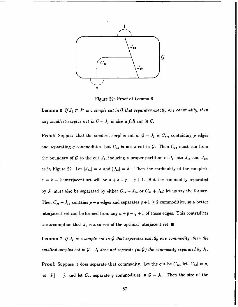
1

I1

Ji.

Cs.jib

\~/

q

Figure 22: Proof of Lemma 6

Lemma 6 If J1 C J" is a simple cut in Q that separates exactly one commodity, then

any smallest-surplus cut in g - J1 is also a full cut in g.

Proof: Suppose that the smallest-surplus cut in ! - J1 is C,., containing p edges

and separating q commodities, but C5, is not a cut in g. Then C,, must run from

the boundary of g to the cut J1 , inducing a proper partition of J1 into Jla and Jib,

as in Figure 22. Let IJJ1. = a and IJ bI = b. Then the cardinality of the complete

r = k - 2 interjacent set will be a + b + p - q + 1. But the commodity separated

by J, must also be separated by either C,, + J10 or C,, + Jib; let us siy the former,

Then Cs, + Jla contains p + a edges and separates q + 1 > 2 commodities, so a better

interjacent set can be formed from any a + p - q + 1 of those edges. This contradicts

the assumption that J, is a subset of the optimal interjacent set. M

Lemma 7 If JI is a simple cut in 9 that separates exactly one commodity, then the

smallest-surplus cut in 9 - J, does not separate (in 9) the commodity separated by JI.

Proof: Suppose it does separate that commodity. Let the cut be Ce,, let IC..I = p,

let IJil = j, and let C,. separate q commodities in ! - J1. Then the size of the

87

optimal interjacent set is j + p - q + 1. But Co. by itself separates q + 1 commodities

in 9, so any p - q + 1 edges from it form a smaller interjacent set than the optimal. M

It is evident from these lemmas that the best interjacent set in the form of Case 2

can be constructed by examining the minimum cuts C in g that separate exactly one

commodity. Each one may be combined with edges from a smallest-surplus cut in

S- C to form a candidate interjacent set. If the optimal solution is of this form, it

will be one of these candidates.

We can conclude that the following algorithm is guaranteed to find an optimal

solution to any UeEP*BN PMCC problem with r = k - 2.

Algorithm 7 ( UeEP*BN r = k - 2 PMCC)

input: g for a UeEP*BN problem with r = k - 2

output: cardinality of a minimum interjacent set

begin

(1) Find the surpluses of every minimum cut that separates a set of consecutive

terminals from its complement in T.

(2) Examine all cuts with the smallest surplus si. If any one of them separates

two or more commodities, then Jopt = s, + 2. Go to Step 5.

(3) Otherwise:

(3a) Find the smallest surplus S2 among all cuts separating two or more

commodities. Set J 2 = 82 + 2.

(3b) For each cut Ci separating exactly one commodity, find the cut with

the smallest surplus si that separates only commodities on one side of

C,, and set Jc, = ICil + si + 1. Set J3 = min{Jc. }.

(4) set Jopt = min{J 2,J 3}

(5) return Jopt

end

The main work in thijq algorilhin is in Step 1, whe-c mninimui cuts must bc found for

88

each partition of T into two consecutive sets. These cuts are equivalent to shortest

paths between separation vertices in gD, (a planar graph). There are 0(k 2 ) such

shortest paths, and if each can be found in 0(-), then the complexity of the algorithm

is 0(-yk 2 ). Alternatively, if the all-pairs shortest paths problem is O(a), this algorithm

is also O(a). We also have the following theorem.

Theorem 2 The r = k - 2 partial multicommodity edge-cut problem with edge

disjoint remaining paths in a T-planar non-crossing graph (UeEP*BN) is polyno-

mially bounded.

Proof: Algorithm 7 gives a polynomial procedure for this problem. m

Unfortunately, this method does not generalize easily to the case in which r < k-3.

The optimal interjacent set J" can be partitioned into J3, J2, and J1 , where J, is a

minimal interjacent set for r = k - 1 and J, + J 2 is minimal for r = k - 2, but there is

no good characterization for 9 - (J1 + J 2 ), a graph in which all but two commodities

can be disjointly connected. Such a characterization needs to be developed before it

will be possible to show a minimal way to achieve it.

However, it is possible to solve a UeEP*BN problem for other values of r when r

is small. This is the subject of the next section.

6.4 The Case of r = 1

Suppose a set of edges J is removed from a T-planar non-crossing multicommodity

flow graph Q, and suppose that in 7? = Q - J only one disjoint si-ti path exists. 1?

may be made up of any number of components, but all save one of them will have

89

no si-ti paths at all. The remaining component V' may have many si-t; paths, but

no two can be disjoint for different values of i. Those commodities that have both

terminals in that component will have them in non-crossing order on its boundary,

since that is how the terminals are distributed in G and the removal of edges will not

change this. In order to characterize such components, then, we need to know the

properties of a U--P*BN multicommodity flow graph in which many components

may be present, but only one disjoint path at a time can be drawn for them. Such a

graph will be called a one-disjoint-path graph.

A graph can be a one-disjoint-path graph because only one commodity has both

terminals in it. Another possibility is that multiple commodities are present, but

a single edge lies on every si-ti path, preventing more than one disjoint path. This

edge will be a bridge connecting two components, each of which contains one terminal

for each commodity. (The edge cannot be in any circuit because the circuit would

provide an alternate si-ti path.) However, these two possibilities do not account for

all one-disjoint-path graphs, as Figure 23 shows. The graph in this figure has three

edges such that every si-ti path contains two of them, so that any two of these edges

constitute an FMCC for the graph. Such edges will be called the three critical edges

of a one-disjoint-path graph. The three possibilities mentioned above characterize all

one-disjoint-path graphs.

Theorem 3 A connected T-planar multicommodity flow graph R' with its terminals

in non-crossing order is a one-disjoint-path graph if and only if at least one of the

following statements is true:

90

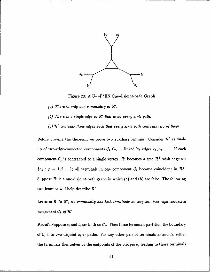
t3 31

S3

t2 S2

Figure 23: A U--P*BN One-disjoint-path Graph

(a) There is only one commodity in V'.

(b) There is a single edge in 1?' that is on every si-ti path.

(c) V' contains three edges such that every si-ti path contains two of them.

Before proving the theorem, we prove two auxiliary lemmas. Consider '1?' as made

up of two-edge-connected components C1,C2.... linked by edges el, e2 , .. . . If each

component C, is contracted to a single vertex, 1?' becomes a tree JZT with edge set

{ep : p = 1,2,.. .}; all terminals in one component Cj become coincident in 1ZT.

Suppose 1?' is a one-disjoint-path graph in which (a) and (b) are false. The following

two lemmas will help describe V?'.

Lemma 8 In V', no commodity has both terminals on any one two-edge-connected

component Cj of 1?'

Proof: Suppose si and ti are both on Cj. Then these terminals partition the boundary

of C, into two disjoint si-ti paths. For any other pair of terminals st and t1, either

the terminals themselves or the endpoints of the bridges e, leading to those terminals

91

must both lie on the same si-ti path. This is because the terminals are in non-crossing

order. Therefore there is an st-tt path that uses only a portion of Cj that is a subset

of one of the two si-ti paths in Ci's boundary. This will be entirely disjoint from the

other si-ti path, a contradiction. n

Lemma 9 In W', every two si-ti paths for distinct commodities share at least one

bridge edge ep.

Proof: Suppose paths Pi (from si to ti) and Pt (from st to ti) share no bridge edges.

Then they must share an edge in a two-edge-connected component Ci. Around the

boundary of Ci there must be four vertices (not necessarily all distinct), each of which

is either one of the terminals si, ti, st, t1, or the endvertex of a unique bridge edge

leading to one of these terminals. By cross-freeness, the four vertices must be in non-

crossing order when a bridge edge endvertex is regarded as representing the terminal

to which it leads. The boundary of Ci will provide disjoint paths linking si to ti and

st to tt. This contradicts the supposition that V' is a one-disjoint-path graph. m

Proof of Theorem: Clearly the truth of (a), (b), and/or (c) implies that 7?' is a

one-disjoint-path graph. The proof is completed by showing that if V' is such a graph

and (a) and (b) are false, then (c) must be true.

In view of the two lemmas, if V' is a one-disjoint-path graph with (a) and (b) false,

then so is the tree RIT formed by contracting all its two-edge-connected components.

Every si-ti path in 7V. has a corresponding path in RTI. Any two paths that are

disjoint in 7V will be disjoint in JZT , and any two paths for distinct commodities

that share an edge in V? will share an edge in 7ZT. So if any si-ti path in 7?! shares

92

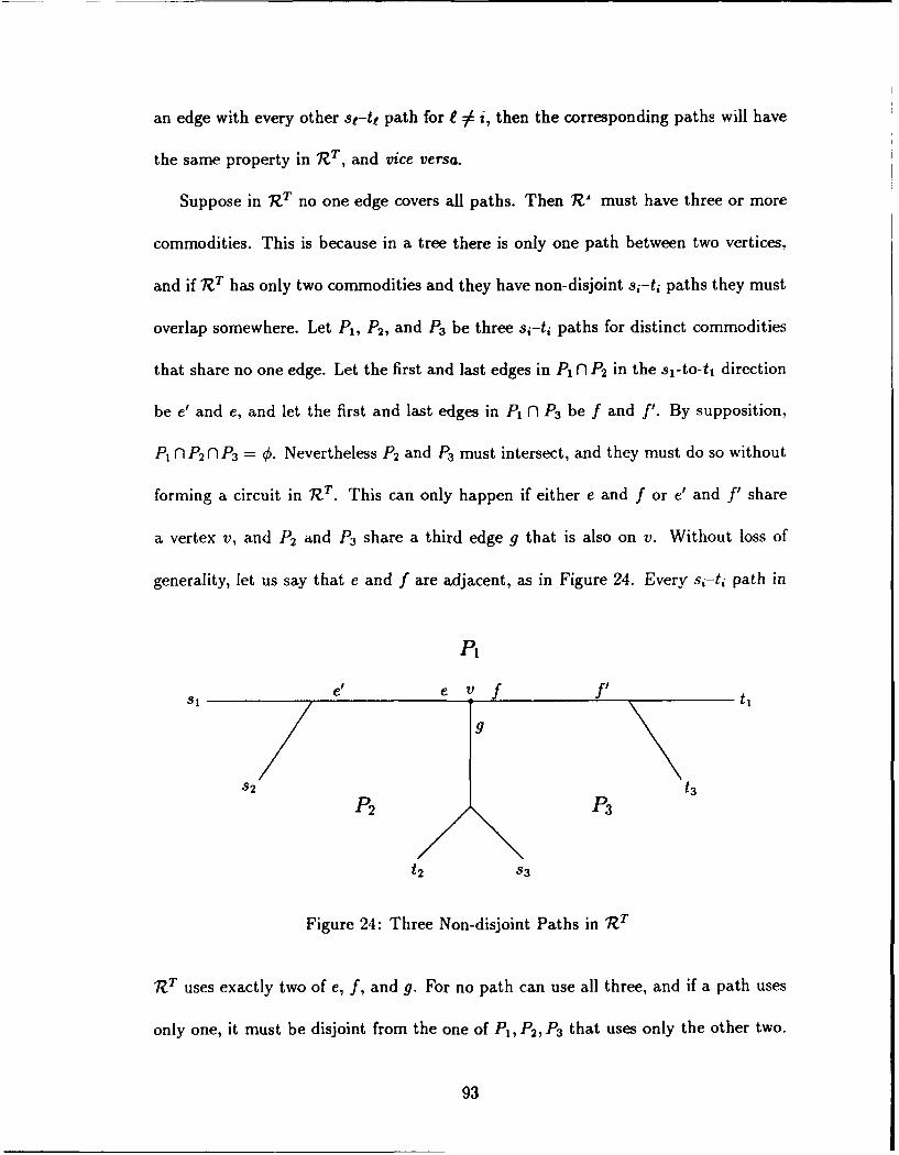
an edge with every other st-tt path for f 3 i, then the corresponding paths will have

the same property in R.T, and vice versa.

Suppose in RIT no one edge covers all paths. Then R1' must have three or more

commodities. This is because in a tree there is only one path between two vertices,

and if JZT has only two commodities and they have non-disjoint si-ti paths they must

overlap somewhere. Let P1 , P2, and P3 be three si-ti paths for distinct commodities

that share no one edge. Let the first and last edges in P1 n P2 in the sl-to-tl direction

be e' and e, and let the first and last edges in P1 nl P3 be f and f'. By supposition,

PI n P2 n P3 = 0. Nevertheless P2 and P3 must intersect, and they must do so without

forming a circuit in ITT. This can only happen if either e and f or e' and f' share

a vertex v, and P2 and P3 share a third edge g that is also on v. Without loss of

generality, let us say that e and f are adjacent, as in Figure 24. Every si-ti path in

P1

e' e V f f'

g

S2 t3

P2 P3

t 2 S3

Figure 24: Three Non-disjoint Paths in JZT

TZT uses exactly two of e, f, and g. For no path can use all three, and if a path uses

only one, it must be disjoint from the one of PI, P2, P3 that uses only the other two.

93

If a path uses none of e, f, and g, then it must be confined to at most one of the

three branches from v that start with these edges, so it will also be disjoint from one

of P1, P2, P3.

Therefore every si-ti path in 1T contains two of e, f, and g, which correspond to

three bridge edges of VI. Since every si-ti path in VI goes through the same bridge

edges as the corresponding path in 1ZT, these three edges in V' cover all si-ti paths.

with each path containing at least two of them. This completes the proof of the

therorem. m

If a one-disjoint-path graph VI is in form (c), we can further assume that no terminals

are in the two-edge-connected component of VI that includes endvertices of all the

critical edges. In 7ZT, such a terminal would be the common endvertex v of the critical

edges e, f, and g, and the terminal's mate would have to be on one of the branches

from v, so that the path to it would be disjoint from at least one of P1, P2, P3 (see

Figure 24).

We now have a complete description of the forms 1Z might take. If J is optimal,

it has exactly one component with si-ti paths, and that component either contains

both terminals for only one commodity, contains a bridge that separates all its com-

modities, or contains three edges two of which are on all paths. Let us call these

the one-commodity, bottleneck, and trifid forms, respectively. If 1? has more than one

component, then the one component containing si-ti paths can also be described by

these terms. If 1Z is in one-commodity form when J is optimal, then J can be found

by solving an FMCC problem in 9 with the commodity in queiii, deleted. If RZ is in

94

bottleneck form, then J can be found by solving an FMCC problem with the bridge

edge removed. We need a method for finding J if 1? is in trifid form.

Let us suppose that for some T-planar non-crossing graph 1 the optimal r = 1

interjacent set J leaves JZ in trifid form. This means that IZ has a component 1?'

that contains three edges, two of which are on every si-ti path in V?!. Let Y' be the

subset of J consisting of edges with both endvertices in V?'. The the role of J - Y

is to separate "?' from the rest of !g (and possibly to subdiviG'e the latter), while J'

partially divides 1?' to make it a trifid one-disjoint-path graph. Call Y' a trifid cut in

1?' (see Figure 25).

j' ~Cla or

-- = trifid partial multicommodity cut Jc = critical edge

j' = part of trifid cut J' (one of three)

Figure 25: Trifid Cut as Part of a PMCC

Let us suppose that 1Z consists of a single trifid component 1?', so that J .1'.

95

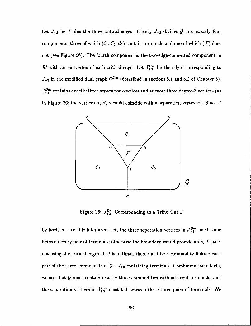
Let J+ 3 be J plus the three critical edges. Clearly J+3 divides g into exactly four

components, three of which (C1 , C2, C3 ) contain terminals and one of which (.F) does

not (see Figure 26). The fourth component is the two-edge-connected component in

R' with an endvertex of each critical edge. Let j7' be the edges corresponding to

J+3 in the modified dual graph !Dm (described in sections 5.1 and 5.2 of Chapter 5).

d+34,, contains exactly three separation-ver'tices and at most three degree-3 vertices (as

in Figure 26; the vertices a, /, -y could coincide with a separation-vertex o,). Since J

U 0*

Cl

a F

C2 7

Figure 26: JDL, Corresponding to a Trifid Cut J

by itself is a feasible interjacent set, the three separation-vertices in J+DI, must come

between every pair of terminals; otherwise the boundary would provide an si-ti path

not using the critical edges. If J is optimal, there must be a commodity linking each

pair of the three components of ! - J+ 3 containing terminals. Combining these facts,

we see that ! must contain exactly three commodities with adjacent terminals, and

the separation-vertices in .+3 must fall between these three pairs of terminals. We

96

call these the key separation-vertices for this problem.

The smallest four-..ay cut in the form of .43 could be found by testing each

possible trio of branch points a, /3, - finding the shortest paths in gDm between

each pair of them and between each one and the three key separation-vertices. The

object would be to find the selection of a, /P, and /, and their assignment to key

separation-vertices, such that the sum of all six distances is minimized. The optimal

trifid cut would then be the sum minus three edges, lacking one edge corresponding

to the edges in paths af3, 0-y, and -ya. But suppose the longest of thses paths is aot.

Then the four-way cut, minus a/3, minus any one edge in 0-y or ya, is also a valid

r = 1 interjacent set, but not a trifid cut. So unless the longest of those paths is only

one edge long, the trifid cut will not be uniquely optimal. And since each component

of the four-way cut must be nonempty, a, /3, and - cannot coincide. Therefore a/3,

,3-y, and -ya must each contain exactly one edge. So if a trifid cut is uniquely minimal,

we can find it by testing every triangle in gDm. (This corresponds to every set of

three edges in 9 that separates a component with no terminals from the rest of the

graph.) We simply find the shortest distance from each of the triangle's vertices to

the three key separation-verticc.s. The selection of a triangle and assignment of its

vertices to key separation-vertices that produces the smallest sum of distances must

correspond to the minimum trifid cut.

The following lemma shows that a trifid cut can also be found by finding a full

multicommodity cut in a modification of g.

Lemma 10 Suppose in a T-planar non-crossing multicommodity flow graph g the

97

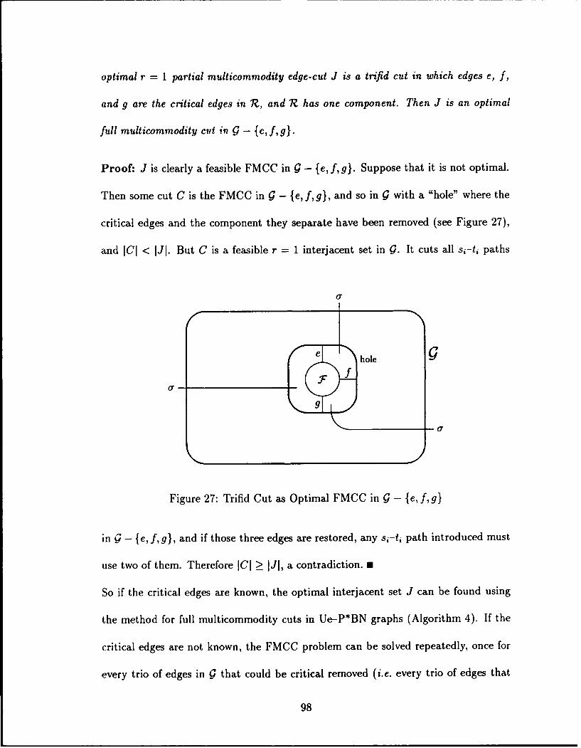
optimal r = 1 partial multicommodity edge-cut J is a trifid cut in which edges e, f,

and g are the critical edges in 1?, and R has one component. Then J is an optimal

full multicommodity cut in 9 - {e, f,g}.

Proof: J is clearly a feasible FMCC in 9- {e, f,g}. Suppose that it is not optimal.

Then some cut C is the FMCC in 9 - {e, f, g}, and so in g with a "hole" where the

critical edges and the component they separate have been removed (see Figure 27),

and ICl < IJI. But C is a feasible r = 1 interjacent set in g. It cuts all si-ti paths

or

e hole 1.F

or"

Figure 27: Trifid Cut as Optimal FMCC in C - {e, f, g}

in - {e, f,g}, and if those three edges are restored, any si-ti path introduced must

use two of them. Therefore ICI Ž_ JJJ, a contradiction. 0

So if the critical edges are known, the optimal interjacent set J can be found using

the method for full multicommodity cuts in Ue-P*BN graphs (Algorithm 4). If the

critical edges are not known, the FMCC problem can be solved repeatedly, once for

every trio of edges in C that could be critical removed (i.e. every trio of edges that

98

separates a component with no terminals). This is clearly a polynomially bounded

procedure.

Now let us turn to the problem of finding a UeEP*BN r = 1 PMCC J when

1? may have more than one component, assuming only that J leaves a component

in trifid form. First let us suppose that the critical edges are known. Let g' be

the supply graph g with these edges removed (disconnecting and in effect removing

a component F of 9 and leaving a hole-see Figure 25), and let C' be an optimal

FMCC in !'. As in the proof of the previous proposition, we can note that C' is also

a feasible PMCC in 9, that J is a feasible FMCC in 9', and that IC'I = IJI. In fact

C' must contain a trifid cut in 9, just like J. If restoring the critical edges and F

to !' - C' introduces no paths, then C' minus any edge is a feasible PMCC in 9,

contradicting [C'[ = fJ[. If it introduces paths, each path must use two of the critical

edges, because no terminals are in F. Thus C' leaves a component of g - C' in trifid

form, and with the same critical edges as J, and C' and J are in this sense equivalent.

If we use Algorithm 4 to find the FMCC C' in 9', we will have the optimal PMCC

in !.

Suppose that the critical edges are not known. There is a polynomial number of

candidate trios, and we need only consider those trios that scparate some component

F7 containing no terminals from the rest of Q. The optimal interjacent set can be

found by solving the FMCC problem in g with each candidate trio removed in turn.

At this point we have a method for finding the optimal interjacent set J for any

UeEP*BN PMCC problem r = 1, whether the component of 1Z containing paths is

99

of the one-commodity, bottleneck, or trifid type. The following algorithm (presented

in outline) can solve in polynomial time a general problem of this type.

Algorithm 8 ( UeEP*BN r = 1 PMCC)

input: 9 for a UeEP*BN problem with r = 1output: cardinality of a minimum interjacent set

begin

(1) Do k FMCC problems, deleting one commodity from consideration each time.

This is guaranteed to find Jopt if it leaves 1Z in one-commodity form.

(2) Do IEl FMCC problems, deleting one edge from g each time. This is guaran-

teed to find Jopt if it leaves 1? in bottleneck form.

(3) For every set F of three edges that separate g into two components, one ofwhich has no terminals, find the optimal FMCC in Q - F. This will find Jopt

if it leaves 1Z in trifid form.

(4) Compare the FMCCs in steps 1, 2, and 3, and set Jopt to the cardinality of

the smallest.

(5) return Jopt

end

The algorithm requires solving O(k + in3 ) FMCC problems (where m = JEl). Since

we have Algorithm 4 to solve these in O(a + k4 + fk 3 + f 2 k2) (see p. 73), we have a

polynomial bound for Algorithm 8 also. This gives us the following theorem.

Theorem 4 The r = 1 partial multicommodity edge-cut problem with edge-disjoint

remaining paths in a T-planar non-crossing graph (case UeEP*BN) is polynomially

bounded.

Proof: Algorithm 8 gives a polynomial procedure for this problem. a

It seems likely that a similar approach can find a polynomially bounded algorithm

for any fixed r. However, it does not look like the solution will be elegant. For

100

instance, with r = 2 we can have in 1R two components with si-ti paths, and each of

them may be in one-commodity, bottleneck, or trifid form. Also, TZ may have only

one component with si-ti paths, but so configured that two disjoint paths and no

more are possible. Clearly a large number of cases will need to be evaluated.

101

7 THE EXTENSION TO VERTEX-CUTS

Some of the important results developed in Chapter 5 and Chapter 6 for multi-

commodity edge-cuts can be extended to vertex-cuts. This chapter shows how this is

done. It includes the following:

§ 7.1 A polynomial algorithm for the weighted T-planar multiterminal vertex-cut problem (cf. Corollary 3)

§7.2 A polynomial algorithm for the weighted T-planar multicommodityvertex-cut problem when the number of commodities k is fixed (cf. Al-gorithm 2)

§ 7.3 Proofs that restricted versions of the T-planar multicommodity vertex-cut problem are NP-hard when k is part of the input (cf. Propositions 10and 11)

§7.4 A polynomial algorithm for the weighted T-planar non-crossing multi-commodity vertex-cut problem (cf. Algorithm 4)

§ 7.5 A polynomial algorithm for the T-planar partial multicommodity vertex-cut vertex-disjoint problem when r = k - 1 (cf. Algorithm 6)

The general method for these results is to construct a sort of dual graph to ! that

plays the role of the modified geometric-dual G D, in the Ue-PB results. This graph

will be called a "face-dual" or gF. There is a correspondence between paths in gF

and vertex-cuts in Q. The correspondence is not as simple as the direct one-to-one

correspondence between paths in QD, and cut-sets in Q, but it is good enough for

the purposes of the algorithms. Once it is established, the methods used in Chapter 5

can at once be seen to apply. The construction of G F and the demonstration of

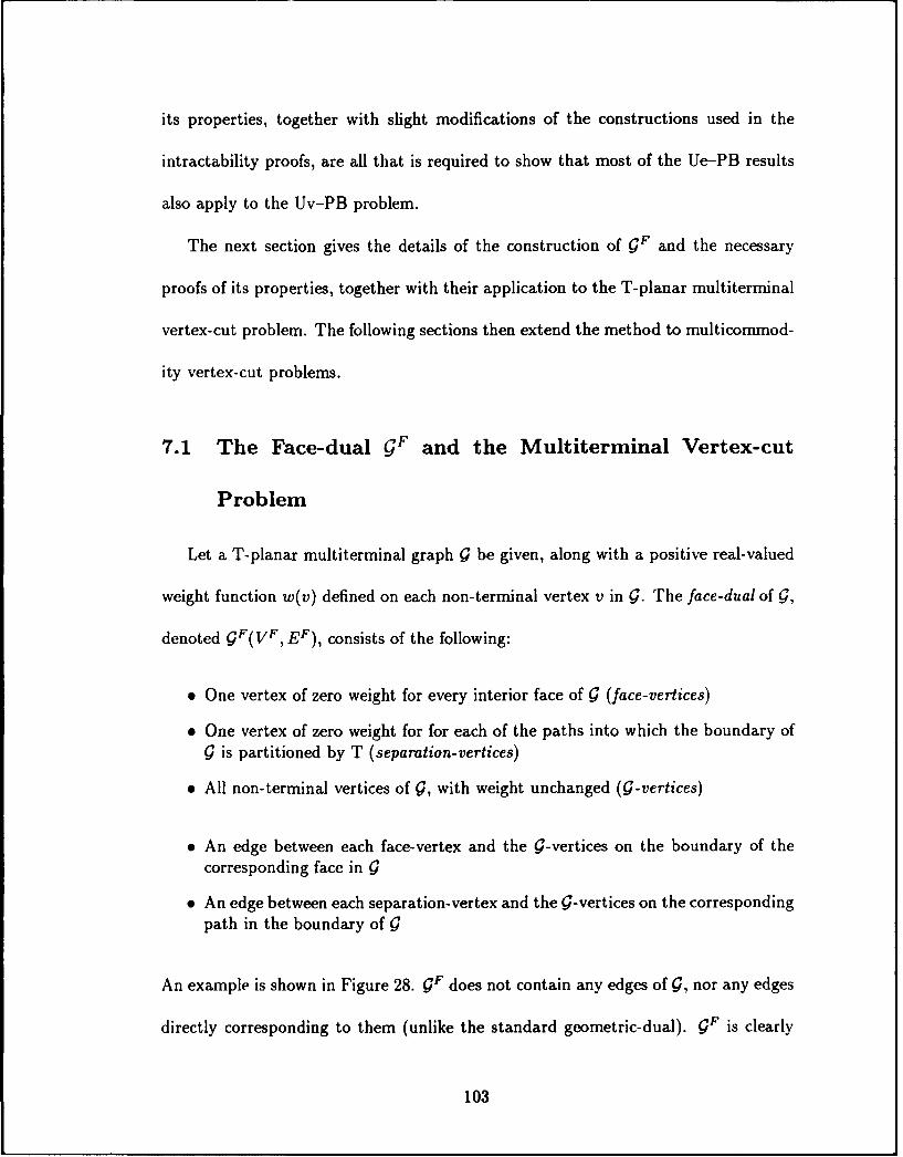
its properties, together with slight modifications of the constructions used in the

intractability proofs, are all that is required to show that most of the Ue-PB results

also apply to the Uv-PB problem.

The next section gives the details of the construction of gF and the necessary

proofs of its properties, together with their application to the T-planar multiterminal

vertex-cut problem. The following sections then extend the method to multicommod-

ity vertex-cut problems.

7.1 The Face-dual gF and the Multiterminal Vertex-cut

Problem

Let a T-planar multiterminal graph Q be given, along with a positive real-valued

weight function w(v) defined on each non-terminal vertex v in G. The face-dual of g,

denoted gF(vF, EF), consists of the following:

"* One vertex of zero weight for every interior face of g (face-vertices)

"* One vertex of zero weight for for each of the paths into which the boundary ofg is partitioned by T (separation-vertices)

"* All non-terminal vertices of g, with weight unchanged (G-vertices)

"* An edge between each face-vertex and the g-vertices on the boundary of thecorresponding face in !

"* An edge between each separation-vertex and the g-vertices on the correspondingpath in the boundary of Q

An example is shown in Figure 28. gF does not contain any edges of 9, nor any edges

directly corresponding to them (unlike the standard geometric-dual). gF" is clearly

103

0

I/

\ //

\ /

01

Figure 28: The Face-dual gF (Example)

planar. It is also bipartite, since every edge connects a g-vertex with either a face or a

separation-vertex. Any path in gF that connects exactly two separation-vertices will

partition the terminals into two consecutive sets. Such a path contains half as many

g-vertices as edges. These g-vertices will form a vertex-cut in g, since by planarity

any path in g between terminals separated by such a path in 9F will have to use one

of those vertices. However, such a vertex-cut will not necessarily be minimal. On the

other hand, each minimal vertex-cut in g corresponds to a path in gF between two

separation-vertices, as the following proposition shows.

Proposition 15 Each minimal vertex-cut between the members of a 2-partition of

T into consecutive sets corresponds (not necessarily uniquely) to a path in gF be-

tween two separation-vertices, and every such path in QF corresponds to a vertex-cut

(unique, but not necessarily minimal) in g.

Proof: Planarity ensures that the unique set of g-vertices on any such path in gF

104

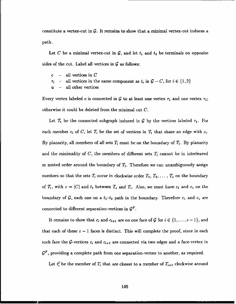
constitute a vertex-cut in !. It remains to show that a minimal vertex-cut induces a

path.

Let C be a minimal vertex-cut in G, and let tj and t2 be terminals on opposite

sides of the cut. Label all vertices in Q as follows:

c - all vertices in C

ri - all vertices in the same component as ti in ! - C, for i E {1,2}u - all other vertices

Every vertex labeled c is connected in G to at least one vertex T, and one vertex T2 ;

otherwise it could be deleted from the minimal cut C.

Let T1 be the connected subgraph induced in ! by the vertices labeled r1 . For

each member ci of C, let Ti be the set of vertices in T1 that share an edge with ci.

By planarity, all members of all sets Ti must be on the boundary of T1 . By planarity

and the minimality of C, the members of different sets T, cannot be in interleaved

or nested order around the boundary of T1. Therefore we can unambiguously assign

numbers so that the sets Ti occur in clockwise order T1, T2, ... , T, on the boundary

of T1, with z = IC1 and t1 between T. and T1. Also, we must have cl and c, on the

boundary of Q, each one on a tl-t 2 path in the boundary. Therefore cl and c. are

connected to different separation-vertices in gF.

It remains to show that ci and ci+l are on one face ofg for i E {1,...,z- 1}, and

that each of these z - 1 faces is distinct. This will complete the proof, since in each

such face the g-vertices ci and cj+1 are connected via two edges and a face-vertex in

gF, providing a complete path from one separation-vertex to another, as required.

Let tf be the member of T, that are closest to a member of T,+j clockwise around

105

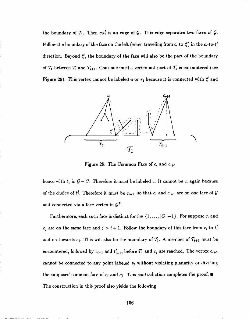
the boundary of T1. Then cit. is an edge of g. This edge separates two faces of g.

Follow the boundary of the face on the left (when traveling from Ci to tf) in the c,-to-t-

direction. Beyond t., the boundary of the face will also be the part of the boundary

of T, between T, and Ti+i. Continue until a vertex not part of T1 is encountered (see

Figure 29). This vertex cannot be labeled u or -r2 because it is connected with t- and

c1 4i+1

Ti Ti+1

Figure 29: The Common Face of ci and Cj+l

hence with tj in -C. Therefore it must be labeled c. It cannot be ci again because

of the choice of tft. Therefore it must be cj+j, so that ci and cj+j are on one face of

and connected via a face-vertex in 9'.

Furthermore, each such face is distinct for i E {1,.. IC- 11. For suppose ci and

cj are on the same face and j > i + 1. Follow the boundary of this face from ci to if

and on towards cj. This will also be the boundary of Ti. A member of Tj+j must be

encountered, followed by cj+j and tf+,, before Tj and cj are reached. The vertex cj+j

cannot be connected to any point labeled r2 without violating planarity or divi~ling

the supposed common face of ci and ej. This contradiction completes the proof. M

The construction in this proof also yields the following:

106

Corollary 4 A minimal vertex-cut in 9 of cardinality p corresponds to a path in gF

that contains 2p edges.

Let the weighted-length of a path in 9F be the sum of the weights of the 9-vertices

on the path. Then the following proposition also holds.

Proposition 16 A minimum-weighted-length path between two separation-vertices in

gF induces a minimum-weight vertex-cut in Q between a set of consecutive terminals

and its complement in T.

Proof: The separation-vertices at the ends of such a path induce a partition of T

into two consecutive sets, and the 9-vertices on the path form a vertex-cut between

these sets with the same total weight as the path's length. These vertices are a

minimum-weight vertex-cut. For suppose a minimal vertex-cut with smaller total

weight existed. Then the construction in the proof of Proposition 15 would provide

a path between the same separation-vertices, and so partitioning T in the same way,

and containing only a-vertices from the smaller cut, so this path would be shorter

than the supposed minimum. n

The T-planar vertex MTC problem is this: for some set of k vertices on the

boundary of a planar graph Q, find the set of other vertices of minimum weight

whose removal from g will disconnect each terminal from each of the others. As in

Section 5.1, we will reformulate the problem into that of finding a tree in gF such that

the C-vertices in the tree are exactly the minimum-weight multiterminal vertex-cut

in C. To ensure that this is possible, we need the following proposition.

107

Proposition 17 Given any minimal multiterminal vertex-cut C in a T-planar graph

9, a corresponding tree in GF exists that includes all separation-vertices and all and

only the G-vertices in the set C.

Proof: The following procedure will construct the required tree:

1. Find a minimal subset of C that separates two terminals tl and t2 .

2. Using the construction in the proof of Proposition 15, find a corresponding pathin gF between two separation-vertices.

3. Repeat steps 1 and 2 for each distinct unordered pair of terminals drawn fromT.

4. Let T be the union of all k(k - 1) paths found in this way. Then T is asubgraph of GF, it includes all and only the g-vertices from C, and it includesall separation vertices.

5. If T includes a cycle, delete any edge in the cycle. Repeat until no cycles remain.

6. If 7T includes a face-vertex as an endvertex after Step 5, delete it and theassociated edge.

T cannot have a G-vertex as a degree-1 vertex: without the edge on such a vertex

it would still contain paths separating all pairs of terminals, so the vertex would be

superfluous in the supposed minimal MTC C. The tree constructed by this proce-

dure will not necessarily be the minimum tree on the separation-vertices, nor will it

necessarily be unique. However, it will contain exactly the g-vertices in C. .

We also need to note that a tree on the separation-vertices in gF will correspond

to a unique multiterminal vertex-cut in g, namely the cut consisting of the G-vertices

in the tree. However, there is no guarantee that the minimum-cardinality tree in

gF will correspond to the minimum-cardinality vertex MTC in G: the number of

108

g-vertices in a tree in g' depends on the location of its branch points, i.e. whether

they are at Q-vertices or face-vertices, as well as on the number of edges it has.

Despit. this lack of direct and unique correspondence, trees in gF can still be

examined to find the optimal vertex MTC in G. We know that there is a tree that

corresponds to the every minimal MTC, and we know that an MTC corresponds to

every tree. Furthermore, each tree can be assigned a well-defined weight equal to

the weight of the MTC it induces: simply the sum of the weights of the g-vertices it

contains. Clearly a minimum-weight tree will induce a minimum-weight vertex-cut.

Furthermore, the weight of a tree thus defined is the sum of the weight of its parts.

This all that is needed to apply an algorithm like that of Provan [1988].

To develop the algorithm, we need a few definitions:

w(v) weight of v E VF (zero except for g-vertices) (47)

dV(v, v) length of a minimum-weighted-length path from (48)v to v, excluding weights of v and v (v, v E VF)

Cv([ao,,], v) = weight (excluding w(v)) of a minimum-vertex- (49)weight tree on [ai, aj] and v E VF

BV([ai, aj],v) weight (including w(v)) of a minimum-vertex- (50)weight tree on [ai, aj] and v E VF when v iseither a separation vertex or adjacent to two ormore edges of the tree

(The m subscripts are applied to these Bv and Cv functions for the MTC problem

to distinguish them from the similar functions that will be defined in Section 7.2.) It

can be shown that at any branch point in the desired tree in gF, each edge leads to a

consccutive set of separation-vertices (Provan [1988]; Erickson, Monma, and Veinott

109

[1987]). Because of this, the following recursive functions hold (using the convention

that Ci =- Oaik):

CV([aij, aj],v) = min {w(v) + d(v, v) + BV([ao,.a , v)} (51)yE VF

and for i # j,

BV([uiaj],v) = w(v) + min {Cv([au, a-],v) + C[([a.+,,oj],v)} (52)

This leads to the following algorithm, which takes gF as input and assumes that it

is two-vertex-connected. (If gF is not two-vertex-connected, the algorithm can be

performed on each two-vertex-connected component, treating articulation vertices as

separation-vertices. If 9 itself has a terminal as an articulation vertex, then gF will

have two components, and trees can be found on them separately.)

Algorithm 9 (Weighted Uv-PB MTC)

input: gF for a weighted Uv-PB MTC problem

output: weight of an optimal MTC in

begin

for each v, v E VF

find minimum weighted-length distance dv(v,v)

for each v E VFm and each separation-vertex a,

set C v([aj, o],v) = dV(ai, v)

for Z = 2, ... , k-1for each set [oi, ab] of cardinality i that does not include a,

for every v E VF

compute B' ([oa, ob], v) using (52)

compute C'([a,, •b], v) using (51)

return CVQ([o 2 ,ak],a1)

end

110

The values dv (v, v) can be found by a simple transformation of the node-weighted

problem into an edge-weighted shortest path problem. Since IVFI is O(m), the com-

plexity of this algorithm is thus O(C + m2 k2 ), where C is the complexity of finding all

the minimum weighted-length dv((v, v) in CF.

7.2 The T-Planar Multicommodity Vertex-cut Problem

with k Fixed

This section will address the problem of finding minimum-weight full multicom-

modity vertex-cuts in T-planar graphs. The development will only be sketched out.

since it is essentially identical to that for the Ue-PB problem addressed in Section 5.2

(p. 43). The only difference is that the face-dual gF plays the role of the modified

geometric-dual gCm. The same labeling conventions are taken when using the face-

dual in a multicommodity problem as were used with the modified geometric-dual:

the distinct terminal vertices in g are labeled in order clockwise order from a, to a.,

and the separation-vertices in CF are likewise numbered, so that 0', falls between a-

and ,1.

If all the terminals are on the boundary of g, then the optimal FMCC corresponds

to a forest in GC, each tree in which is on some subset of the separation-vertices. Every

vertex-cut in C induces a path between separation-vertices in F.G and every such path

induces a unique vertex-cut. We can conclude that there - in G F of disjoint

trees on subsets of the separation-vertices, such that that . iuces the optimal

vertex FMCC in C. If we define the weight of a tree in CF as the sum of the weights of

111

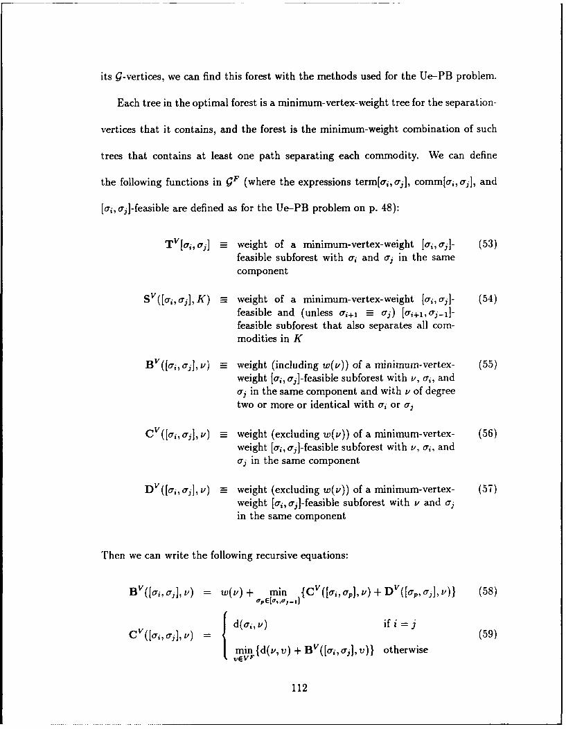
its Q-vertices, we can find this forest with the methods used for the Ue-PB problem.

Each tree in the optimal forest is a minimum-vertex-weight tree for the separation-

vertices that it contains, and the forest is the minimum-weight combination of such

trees that contains at least one path separating each commodity. We can define

the following functions in gF (where the expressions term[ui, aj], comm[a,, aj], and

[ai, aj]-feasible are defined as for the Ue-PB problem on p. 48):

TV[ai, aj] weight of a minimum-vertex-weight [aiaj]- (53)feasible subforest with ai and aj in the samecomponent

SV([a, aj],K) weight of a minimum-vertex-weight [oi, a,]- (54)feasible and (unless i+l a) [ai+=,_-i]-feasible subforest that also separates all com-modities in K

Bv([a, aj],v) weight (including w(v)) of a minimum-vertex- (55)weight [ai, aj]-feasible subforest with v, aj, anda, in the same component and with v of degreetwo or more or identical with ai or aj

CV([ai, aj, v) weight (excluding w(v)) of a minimum-vertex- (56)weight [ai, aj]-feasible subforest with v, ai, andao in the same component

DV([a,, aj],v) weight (excluding w(v)) of a minimum-vertex- (57)weight [ai, a1 ]-feasible subforest with v and ajin the same component

Then we can write the following recursive equations:

BV([a,,aj],,v) = w(v)+ min {CV([a,, ap],v)+DV([ap, aj],v)} (58)ap,•[a ,,aj _d

CV([ai'aj],v) = { d(a,,v) if i=(59)

min {d(v,v) + BV([aj,aj],v)} otherwiseVEVF

112

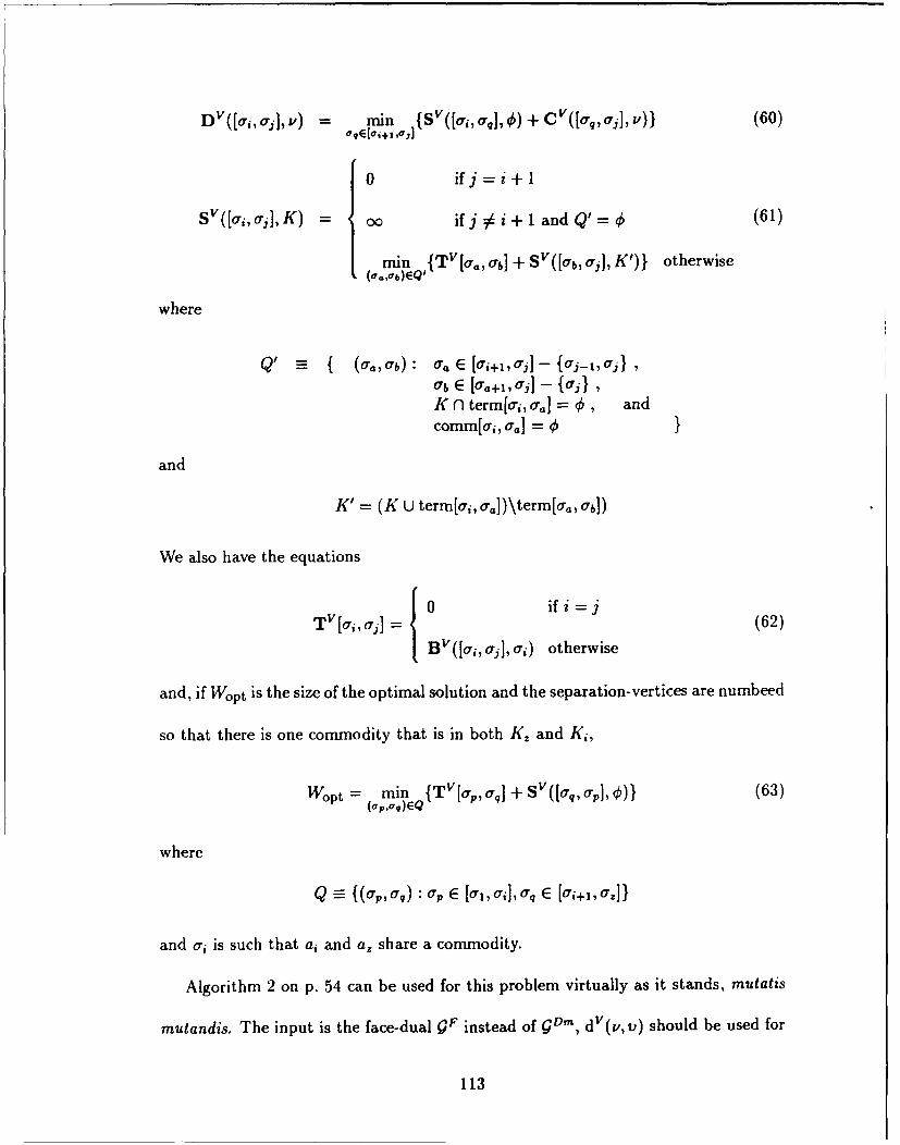
DV(aj,,ailv) = mrin fsV([ai, J],)+CV(a,aj],V)} (60)uq•[u,+z ,oJ]

0 ifj=i+1

SV([:,oaj],K) = oo if j 0 i + 1 and Q'=q (61)

amin {TV[a., ab] + SV([Ob, aj],K')} otherwise(ca,ub)EQ'

where

{ (0.,Uab) : a. E [ai+l,aj] - {fai-1,a} I0rb E [ar+,,aj - {Oj} ,K fl term~o,, a,.] -- €, andcomm[aj,G0] = a

and

K' = (K U term[ai, aI])\term[a,, ab])

We also have the equations

TV [oi, 0] if-- (62)

BV([aI, a],aj) otherwise

and, if Wopt is the size of the optimal solution and the separation-vertices are numbeed

so that there is one commodity that is in both If. and Ki,

Wop t== min {TV[ap,rq]j+SV([o'q,orp],O)} (63)(0cp,aq)EQ

where

or -- ) ap [Or,,ail, Oq E [O,+i,, o]}

and oi is such that ai and a, share a commodity.

Algorithm 2 on p. 54 can be used for this problem virtually as it stands, mutatis

mutandis. The input is the face-dual QF instead of gnm, dV(v,v) should be used for

113

d(v, v), and the V-superscripted versions of functions S, T, B, C, and D should be

used (eqns. (49), (58)-(62)). The complexity is O(( + 2kk4 + mk3 + m2 k2), where all

distances d(v, v) are found in O(C).

7.3 The Intractability of Vertex-cuts when k Varies

This section contains two propositions on the intractability of multicommodity

vertex-cuts in T-planar graphs. The problem is NP-hard even when restricted to rec-

tangular grids with rectangular boundaries. The weighted problem is NP-hard even

when restricted to trees. These results parallel exactly those in the edge-cut case

(Propositions 10 and 11), and the proofs are derived from them.

The vertex-disjoint paths construction problem is not feasible unless the terminals

are in non-crossing order (in which case the FMCC problem is polynomial, as we will

see in the next section); the edge-disjoint paths problem can be feasible regardless of

the order of the terminals. However, it still makes sense to ask what minimum set of

vertices will lie on all si-ti paths, even if a full set of disjoint paths is not possible.

Proposition 18 The unweighted T-planar full multicommodity vertex-cut problem is

NP-hard, even when restricted to rectangular grids with rectangular boundaries.

Outline of Proof: The general method is exactly the same as that for Proposition 10,

which makes the same claim for edge-cuts. A vertex cover problem in a graph with all

vertices of degree 3 is polynomially reduced to a Uv-PB FMCC problem. The same

system of commodities is used: vertex, edge, and connecting. The gadgets must be

modified slightly-see figures 30 and 31. A non-terminal vertex must be left between

114

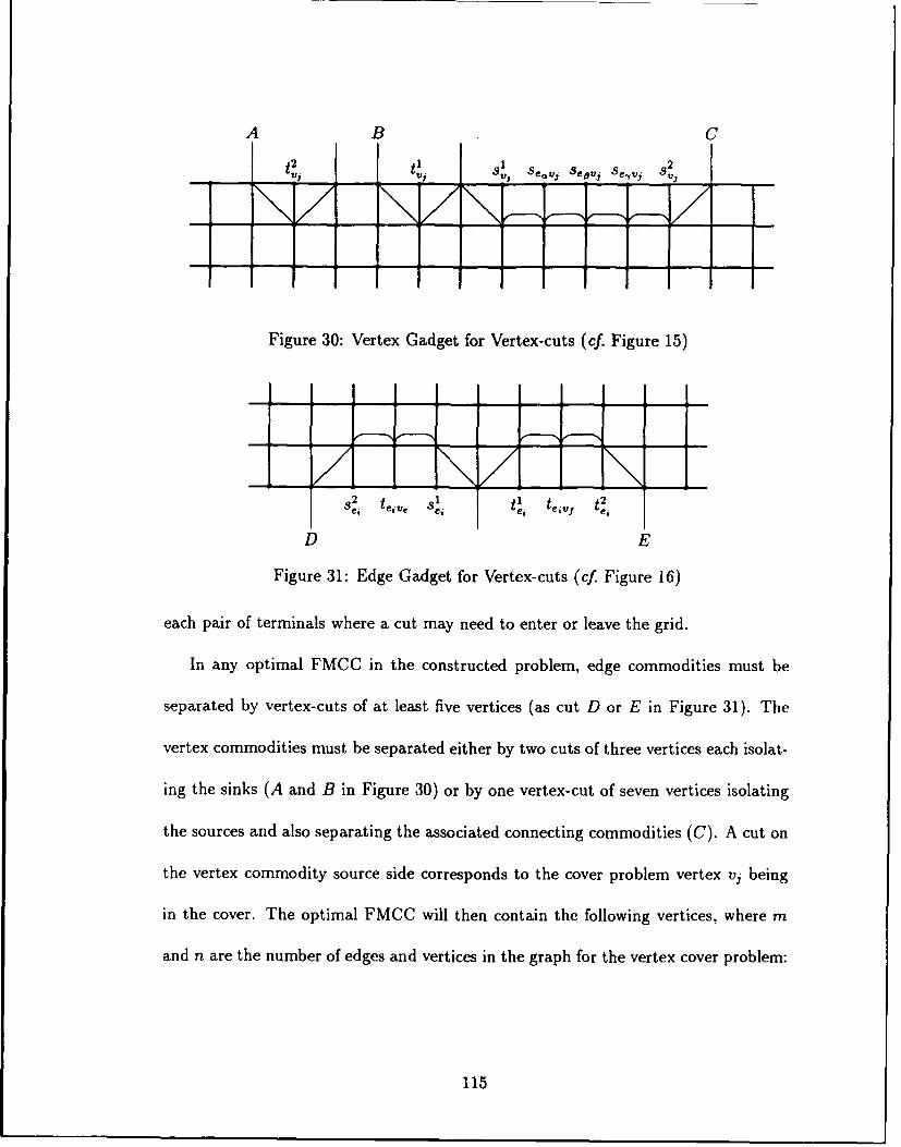
A B C

0v tls eavj Seovj 8e-,vi Sv

Figure 30: Vertex Gadget for Vertex-cuts (cf. Figure 15)

82 •e e 1• •eivy eee ete, t , t

D E

Figure 31: Edge Gadget for Vertex-cuts (cf. Figure 16)

each pair of terminals where a cut may need to enter or leave the grid.

In any optimal FMCC in the constructed problem, edge commodities must be

separated by vertex-cuts of at least five vertices (as cut D or E in Figure 31). The

vertex commodities must be separated either by two cuts of three vertices each isolat-

ing the sinks (A and B in Figure 30) or by one vertex-cut of seven vertices isolating

the sources and also separating the associated connecting commodities (C). A cut on

the vertex commodity source side corresponds to the cover problem vertex vj being

in the cover. The optimal FMCC will then contain the following vertices, where m

and n are the number of edges and vertices in the graph for the vertex cover problem:

115

5 for each of m edge commodities

6 for each of n vertex commodities

1 for each set of three connecting commodities separated by source-sidevertex commodity cuts

There is a vertex cover of size p if and only if there is an FMCC in the constructed

problem of at most 6n + 5m + p vertices. a

Proposition 19 The weighted full multicommodity vertex-cut problem is NP-hard

even when restricted to trees.

Proof: The corresponding edge-cut problem is NP-hard (Proposition 11), and it can

be reduced to the vertex problem by inserting a vertex into each edge with the edge's

weight and assigning an arbitrarily high weight to all other vertices. M

7.4 A Polynomial Case: T-Planar and Non-crossing

A polynomially-bounded algorithm analogous to Algorithm 4 (for the correspond-

ing edge-cut problem) can be developed for T-planar multicommodity vertex-cuts if

the terminals are in non-crossing order. The functions dv, TV, BV, Cv, and Dv func-

tions developed for the Uv-PB problem (Section 7.2) can be used. The SV([ai, rj], K)

function can be modified slightly because it need be calculated only for K = 4': the

"betweenness" argument used in developing Algorithm 4 for Ue-P*BN edge-cuts

(Section 5.5) applies without modification. The formula then becomes:

SV(a, ij. 3], 4) = min {S([a,, a], 4) + T[aug,aOh] + S([ah,aj], 0)) (64)

where

116

Q (u9 , O') :o~g E [o'i+i , 0qJ - 10'Jl""rh E fog+ia] - fj }at least one of Org,h is in [ri+i,op] U [aoq+l,aj] - {oj} }

and ap is such that a member of Kp is also a member of term[ap+i, oj], say in Kq, and

no member of comm[ao, oj] is in term[ac, ap]. Algorithm 4 in Section 5.5 can then be

used for the Uv-P*BN problem, mutatis mutandis: QF used in place of GD, and the

V-superscripted versions of the d, S (eq. 64), T, B, C, and D functions used. The

complexity comes out to O(C + k4 + mk3 + m2 k2). This gives us:

Proposition 20 The weighted T-planar full multicommodity vertex-cut problem is

polynomially bounded if the terminals are restricted to be in non-crossing order.

Proof: Outlined in the preceding paragraph. m

7.5 Partial Multicommodity Vertex-cuts

Just as for edge-cuts, the intractability of the full multicommodity vertex-cut

problem implies an additional constraint (beyond those of Proposition 4 in Chaper 4)

on the tractability of partial vertex cuts. On the other hand, polynomially bounded

algorithms are possible for special configurations. One such algorithm is developed

here, for the UvVPB case with r = k - 1.

The T-planar non-crossing PMCC problem with r = k - 1 can be handled for

vertex-cuts just as it was for edge-cuts in Section 6.2. For the U-VPB disjoint paths

construction problem, cross-freeness and the general cut condition are necessary and

sufficient for the existence of a solution [Robertson and Seymour, 19861. If cross-

freeness does not hold in 9, then the smallest r = k- I interjacent set is the empty set.

117

Suppose that cross-freeness does hold. Removing vertices from Q will not change that

fact. Therefore the optimal interjacent set is the smallest vertex set whose removal

from g will result in a violation of the GCC for some vertex-cut in g. Furthermore,

it is necessary to consider only simple vertex-cuts, since some such minimal cut will

violate the GCC if a compound cut does. Also, if the GCC is violated for any simple

cut, it will be violated as much or more for the minimum vertex-cut that partitions

the boundary in the same way. This suggests the following algorithm, which is the

counterpart of Algorithm 6 for the edge-cut case:

Algorithm 10 ( UvVPB r = k - 1 PMCC)

input: g for a UvVPB problem with r = k - 1output: cardinality of a minimum interjacent set

begin

if ! is not cross-free

return 0

end

set Jopt -- oo

for i = 1 to [IT[/2J

for every set S of i consecutive terminals in T

set p equal to the number of unmatched terminals in S

find the minimum vertex-cut C between S and T - S

set Jopt=min f Jopt, ICI-p+1}

return Joptend

The complexity of this algorithm is 0(bk2 ), where b is the complexity of finding a

minimum vertex-cut in a planar graph. Alternatively, since the cuts C correspond to

shortest paths between separation vertices in gD", the algorithm is O(a), where a is

the complexity of the all-pairs shortest paths problem.

118

If there is a vertex-cut with the smallest surplus in Q that separates two or more

commodities, any surplus-plus-two vertices from that cut will be a feasible r = k - 2

interjacent set. From Lemma 3, we can also say that this interjacent set is optimal.

In fact, we have the following proposition:

Proposition 21 In a T-planar partial multicommodity vertex-cut problem with the

terminals in non-crossing order, suppose that C is a simple vertex-cut that contains

p vertices and separates q commoditie -nd suppose that no vertex-cut in g has a

smaller surplus than C. Suppose further that k- I > r > k-q. Then any p-q+k-r

vertices in C are an optimal interjacent set.

Proof: An interjacent set as descibed is clearly feasible, for it prevents k - r of

the q commodities separated by C from being connected by vertex-disjoint paths.

Optimality has already been shown for the case r = k - 1. Lemma 3 implies that if

a new feasible interjacent set can be found with just one additional vertex when r is

decremented, then that set must be optimal. By induction, each addition of a new

vertex from C to the interjacent set results in a new optimal set for a value of r one

smaller, until C is exhausted. m

119

8 THE SINGLE-SOURCE PROBLEM

An important special case of the partial multicommodity cut problem is the case

in which all commodities have a common source. This is a common situation in a

communications or logistics network, where data or goods may travel from one central

location to a large number of user locations. It turns out that the PMCC problem

is much easier in this case. Even in general graphs, it has a polynomial solution as

long as k, r, or k - r is bounded. The method should be practical for answering such

questions as, "What is the smallest loss of links that will cut off three or more of the

users?"

From the symmetry of the problems, the single-sink problem is equivalent to the

single-source. In an undirected graph the si and ti labels can be interchanged, so all

that is required is that there be one vertex that is a terminal for each commodity.

All these variations will be treated under the name of a single-source problem.

The full multicommodity cut problem (r = 0) is easily solved in the single-source

case. For example, let us take such a problem in a directed graph. A super-sink t' is

added to the digraph, along with the set of terminal arcs {tit' : i = 1,..., k}. Call the

resulting digraph the sink-augmented graph !'. If the terminal arcs are given infinite

weight and all other arcs weight 1, the minimum-weight s-t' cut in Q' will then be the

required FMCC in !. With well-known reformulations, this applies to either directed

or undirected graphs and either edge- or vertex-cuts.

Up to this point in this work only undirected graphs have been considered. In

contrast, this section looks at the single-source problem initially as a directed graph

problem; this is appropriate to the asymmetry between the single source and the

many sinks. We start the development with arc-cuts that leave arc-disjoint paths

(the DeE case) with r = 1 (Section 8.1), and then generalize to handle any value

of r (Section 8.2). Section 8.3 will show how these results can be used with little

modification in undirected graphs, when vertex-cuts are required, or both (UeE, DvV,

and UvV). The next two sections consider the more complicated cross-cases DeV and

DvE: here arcs are to be removed from Q until only r vertex-disjoint paths remain, or

vice versa. The cross-cases are perhaps rarer in actual applications; they are developed

here most fully for the r = 1 case. Finally, the last section in this chapter returns to

undirected and (nearly) T-planar graphs. For this interesting special case, methods

similar to those of Chapter 5 are used to find an algorithm that is polynomially

bounded for unrestricted r and k in the input.

8.1 Arc-cuts, Arc-disjoint paths, r = 1 (DeE)

We consider here the problem: given a multicommodity flow digraph g in which

one node is the source for every commodity, find the smallest set of arcs J whose

removal leaves no more than one arc-disjoint path from the source s to any sink ti. A

practical method for solving this problem comes directly from the following lemma.

Lemma 11 For any feasible solution J to a single-source partial multicommodity cut

121

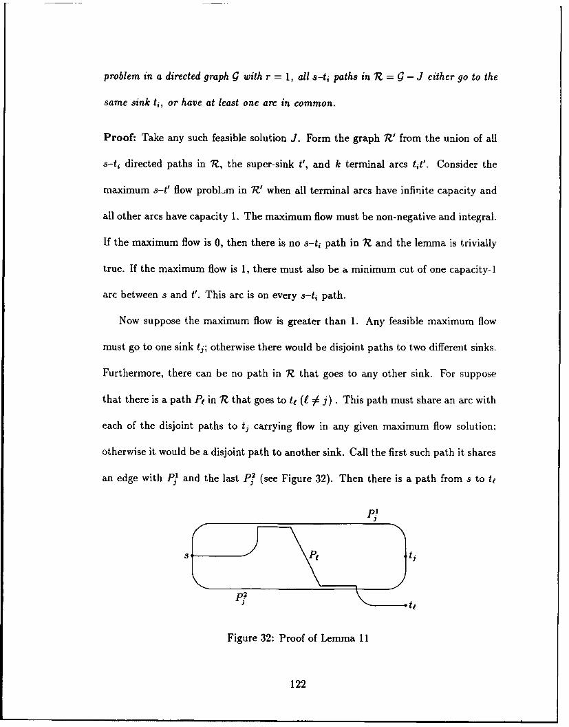
problem in a directed graph G with r = 1, all s-ti paths in R = G - J either go to the

same sink ti, or have at least one arc in common.

Proof: Take any such feasible solution J. Form the graph R' from the union of all

s-ti directed paths in 1R, the super-sink t', and k terminal arcs tit'. Consider the

maximum s-t' flow probl-;m in TV! when all terminal arcs have infinite capacity and

all other arcs have capacity 1. The maximum flow must be non-negative and integral.

If the maximum flow is 0, then there is no s-ti path in X and the lemma is trivially

true. If the maximum flow is 1, there must also be a minimum cut of one capacity-I

arc between s and t'. This arc is on every s-ti path.

Now suppose the maximum flow is greater than 1. Any feasible maximum flow

must go to one sink ti; otherwise there would be disjoint paths to two different sinks.

Furthermore, there can be no path in R that goes to any other sink. For suppose

that there is a path Pt in R1 that goes to tt (1 3 j). This path must share an arc with

each of the disjoint paths to tj carrying flow in any given maximum flow solution;

otherwise it would be a disjoint path to another sink. Call the first such path it shares

an edge with PF and the last P? (see Figure 32). Then there is a path from s to t,

P?

Figure 32: Proof of Lemma 11

122

that follows P until its last common node with Pt, then follows Pt. This path is

disjoint from P] and goes to a different sink, contradicting the feasibility of J. 0

Let G' be G plus t' plus the terminal arcs. Note that in G', any r = 1 PMCC has

the property that it plus at most one additional arc (either an arc of g or one of the

terminal arcs) is a full s-t' cut. Also, any such full cut that uses no more than one of

the terminal arcs can be made into a PMCC by deleting the terminal arc if present,

or by deleting any one of the other arcs if it contains no terminal arc. So we can find

a minimum PMCC J for the r = 1 single-source case by finding the minimum cut C'

in G' (with all arcs, including terminal arcs, at equal weight), with the side condition

that no more than one of the terminal arcs can be in C'. J is then formed from C'

by deleting one of its members (a terminai arc, if present), and IJI = 1C01 - 1.

The side condition is of a combinatorial nature, and adding its linear relaxation

does not necessarily result in a 0/1 solution when finding the minimum cut via the

simplex method. An example is shown in Figure 33. The minimum cut without side

t,

a4

t2

Figure 33: Example of Side Condition Causing a Non-integral Simplex Solution

constraint here is {a6, a7}. If the constraint xa6 + x., < 1 is added, a non-integral cut

123

of size 2.5 results, with x,, = Xa2 = Xa3 = Xa = X"? = 0.5. A proper minimum cut

with side constraint is {a,, a2, a7 }.

Nevertb,-hýss, the problem can still be solved in polynomial time by solving at most

k minimum cut problems in W', in each one excluding all but one of the terminal cuts

by setting their capacities at more than [El. If a general minimum cut problem is

O(ij), the single-source PMCC r = 1 problem is O(77k).

8.2 Generalizing DeE to 1 < r < k

Lemma 11 can be generalized in the following way:

Lemma 12 For any feasible solution J to a single-source partial multicommodity cut

problem in a directed graph g, all s-ti paths in R? = g - J can be partitioned into two

sets such that for some integer p, 0 < p < r, all paths in one set can be covered by p

edges, and all paths in the other go to no more than r - p sinks ti.

Proof: Take any such feasible solution J. Form the graph VZ' from the union of

all s-ti directed paths in 1?, the super-sink t', and k terminal arcs tit'. Consider

the maximum s-t' flow problem in V? when all arcs have capacity 1. The total flow

can be no more than r; otherwise 1Z contains more than r disjoint paths to different

terminals. Therefore the minimum cut in V' is no more than r. Let such a minimum

cut consist of a set P of arcs from 1Z and a set Q of terminal arcs, so that IPI + IQI < r.

Partition all s-ti paths in 1Z into those containing one or more of the arcs in P and

those containing none. The second set of paths must go to one of the IQI sinks

belonging to terminal arcs in C3, otherwise they will not be cut by the minimum cut.

124

With p = IPI, all paths in 1Z have been partitioned as required..

If the interjacent set J is minimal, this can strengthened:

Lemma 13 For any minimal solution J to a single-source partial multicommodity

cut problem in a directed graph g, all s-ti paths in 1Z = G - J can be partitioned into

two sets such that for some integer p, 0 < p < r, all paths in one set can be covered

by p edges, and all paths in the other go to exactly r - p sinks ti.

Proof: By Lemma 11, all paths can be partitioned into two sets such that Set 1 is

covered by p arcs and Set 2 other goes to q distinct sinks, and p + q < r. It remains

to show that if J is optimal then p + q = r.

If p + q < r, there are fewer than r disjoint s-ti paths in 1?: no more than p in

Set 1, plus no more than q in Set 2. Adding one edge to 1Z (i.e. removing one edge

from J) can add no more than one arc-disjoint path, so the number of disjoint paths

will still be feasible if J is reduced by one arc, and it cannot be minimal. a

With a single-source PMCC characterized in this way, there is a natural way to

find the optimal solution. The following algorithm shows how this is done; the proof

of correctness follows. The construction described in the algorithm is illustrated in

Figure 34.

125

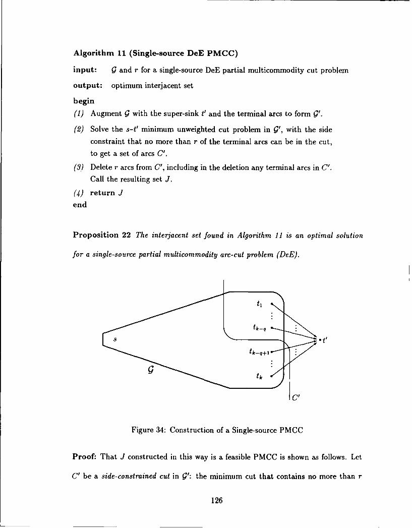
Algorithm 11 (Single-source DeE PMCC)

input: g and r for a single-source DeE partial multicommodity cut problem

output: optimum interjacent set

begin

(1) Augment ! with the super-sink t' and the terminal arcs to form g'.

(2) Solve the s-t' minimum unweighted cut problem in 9', with the side

constraint that no more than r of the terminal arcs can be in the cut,

to get a set of arcs C'.

(3) Delete r arcs from C', including in the deletion any terminal arcs in C'.

Call the resulting set J.

(4) return J

end

Proposition 22 The interjacent set found in Algorithm 11 is an optimal solution

for a single-source partial multicommodity arc-cut problem (DeE).

tSt

CI

Figure 34: Construction of a Single-source PMCC

Proof: That J constructed in this way is a feasible PMCC is shown as follows. Let

C' be a side- constrained cut in V': the minimum cut that contains no more than r

126

terminal arcs. Let C' be partitioned into a set of terminal arcs Q and a set of other

arcs P' = C' n E. Let g(-) = g - P'. Then 9(-) contains paths to IQI = q different

terminals. Let P be a set of any r - q = p arcs in P'. Since adding each arc can

permit no more than one additional s-ti path, 9(-) + P can have no more than r

disjoint s-ti paths. But

g(-)+p = g-(P'-P) = 9-J (65)

showing that J is feasible.

It remains to show that J is optimal. Suppose there is a smaller interjacent set

P, and let 1?* = G - P. By Lemma 12, we can find a set of arcs P* and a set of

terminal arcs Q* such that every s-ti path in T7* contains a member of P* or ends at

a sink corresponding to a member of Q*, and IP*I + IQ'I < r. So in G' the following

is an s-t' cut:

C* = P* + P* + Q* (66)

Also, C" contains IQ*I < r terminal arcs. Since C' is the side-constrained minimum

cut in 9' and IP'J + IQ*I < r,

ICil !5 1C*l = IJ'l + IPlI + IQ*l <- IJ'l + r (67)

But IJI = C'I - r, so

hi < IJil (68)

contradicting the supposition. M

To find the smallest side-constrained cut C', it is only necessary to solve the (k)r

minimum cut problems in C' with each possible set of r terminal arcs at capacity 1,

127

the balance being at infinite capacity. If the smallest side-constrained cut C' uses

fewer than r terminal arcs, it will appear whenever a superset of its terminal arcs is

allowed in the solution.

In solving the (r) minimum cut problems, it is necessary to leave the r

terminal arcs in as capacity-1 arcs eligible to be part of the cut, rather than making

them automatically part of the cut (i.e. by setting them at capacity 0). An example

of this is shown in Figure 35. Using the procedure of Proposition 22, there are three

t I t2

Figure 35: A PMCC Problem with k = 3, r = 2

minimum cut problems to solve, each with one of the three terminal arcs set at infinite

capacity. If the other terminal arcs are set at zero capacity, the best PMCC found is

three arcs. If they are set at capacity 1, the correct PMCC of any two of the three

arcs at a is found.

If r is fixed, (k) is 0(kr ), and so Algorithm 11 is polynomially bounded. If k

is fixed, the algorithm is also bounded, since r < k. If both r and k vary but their

difference is bounded, then the algorithm is bounded by kk-r times the work to find a

minimum cut in a general digraph. Only when k --+ oo, r --+ o, and k - r -+ 0o does

this method of solution increase exponentially. Thus we have the following theorem.

128

Theorem 5 The single-source partial multicommodity arc-cut problem with arc-

disjoint remaining paths (case DeE) is polynomially bounded if r or k - r is bounded.

Proof: The preceding discussion shows that Algorithm 11 is a polynomial method

for this problem. 0

8.3 Generalizing to Cases UeE, DvV, and UvV

With standard reformulations, the method developed in the previous two sections

for partial arc-cuts can also be used for edge-cuts in undirected graphs and for node-

or vertex-cuts. The only restriction is that the disjointness of the remaining paths

must be determined by the same graph elements that make up the cut; the cross-

cases are addressed in following sections. This section shows the applicability of

the last section's method to UeE, to DvV, and finally to UvV single-source partial

multicommodity cuts.

The standard way to reformulate an undirected cut problem as a directed one

is to replace each edge with two oppositely directed arcs. It is well-known that the

minimum arc-cut will never contain a pair of such opposite arcs, and the set of edges

corresponding to the arcs in the minimum directed cut is a minimum undirected cut

of the same cardinality. This reformulation also works for partial multicommodity

cuts, as the following lemma shows.

Lemma 14 Given a single-source partial multicommodity edge-cut problem in an

undirected graph g, let J be the set of edges corresponding to the members of an

optimal solution to the corresponding directed cut problem formed by replacing every

129

edge in ! with two oppositely directed arcs. Then J is an optimal solution to the

original undirected problem.

Proof: Let J be an interjacent set formed as described. J must be feasible, since the

undirected graph cannot have more s-ti paths in it than the corresponding directed

graph. Suppose there is a smaller feasible interjacent set J*. We can apply the

partition-of-paths argument used on the proof of Lemma 12 to show that there must

be in 9 - J" a set of edges P* and a set of terminals Q* such that each s-ti path in

g - J" is covered by either P* or Q*, and IP*I + IQ*I __ r. Let

C' = J* + P" + {tit': ti E Q*} (69)

Then C' is a full s-t' cut in the sink-augmented undirected graph 9', and divides

g' into at least two pieces, one of which contains s and another t'. Let 9d'ir be the

sink-augmented graph for the corresponding directed cut problem, and let Cdjir be the

set of arcs corresponding to C' in the s-to-t' direction. This is well-defined because

of the way C' divides C'. Also, Clir contains 1Q*1 < r terminal arcs, and

ICdiirl = IC'I __ IJ'l+r < IJI+r (70)

But by the method of construction of J and Proposition 22, the smallest such side-

constrained s-t' cut in !lir is of cardinality IJI + r. This is a contradiction. w

The directed node-cut, node-disjoint problem DvV can be reformulated as a ca-

pacitated version of the DeE problem in the standard way by splitting each node into

an in-node and an out-node connected by a capacity-1 node arc; all the other arcs of C

then go from an out-node to an in-node and have infinite capacity. The arguments of

130

lemmas 11 and 12 and Proposition 22 apply equally well to this reformulated problem.

Let 9N be G reformulated as described, and let G' be that digraph augmented with

t' and capacity-i terminal arcs. The optimal partial node-cut must correspond to

the minimum arc-cut in !v that coiisists of only node arcs and terminal arcs, and no

more than r of the latter. This minimum cut can be found by evaluating () such

arc-cuts. Thus the node version of the single-source PMCC problem is polynomially

bounded under the same restrictions as the arc version.

The remaining non-cross-case is UvV. Using the same methods, it is easy to see

that for an optimal J, every s-ti path in 1Z must either be covered by a set of vertices

P or go to a set of sinks Q, with IPI + JQJ = r. Therefore J can be formed from the

smallest s-t' vertex-cut C' in G' that includes no more than r of the k vertices ti: J is

C' less any subset of r vertices that includes all vertices t, in C'. Finding the optimal

solution in the general case requires evaluating (k) minimum vertex-cuts in G'.

We summarize this section in the following theorem.

Theorem 6 The single-source partial multicommodity cut problem with r or k - r

bounded is a polynomially bounded problem for node-cuts and node-disjoint paths in

directed graphs (DvV), and for either edge-cuts and edge-disjoint paths or vertex-cuts

and vertex-disjoint paths in undirected graphs (UeE and UvV).

Proof: Lemma 14 shows that a UeE problem can be reformulated as a DeE problem,

which has been shown to be polynomial under the given restrictions (Theorem 5). The

foregoing discussion shows that DvV and UvV problems can be solved by evaluating

(k) vertex-cut problems, so these cases are also polynomial. v

131

8.4 The Cross-case DeV

We next consider the problem of removing the smallest number of arcs from a

digraph so that there are no more than r node-disjoint paths left between a source s

and distinct members of the set of sinks Iti,... , tk }. This might represent a situation

in a pipeline network in which the factor limiting throughput was pumping capacity at

the nodes, but it is desired to know the consequences of closing some of the lines. We

could imagine a question like, "What is the smallest number of lines closed that will

result in only r of my customers being served?" This problem would be formulated

as a DeV partial multicommodity cut problem.

Let such a PMCC problem be given with r = 1. Without loss of generality we

can assume that s has zero in-degree and all nonterminal nodes have non-zero in- and

out-degrees. The sinks ti must have non-zero in-degree, but may or may not have

out-arcs.

Candidate PMCCs can be found by finding the minimum arc-cuts between s and

each of the k sets of all sinks but one. Suppose that the smallest of these k candidate

PMCCs is of cardinality j. If this size-j candidate is not the optimum PMCC, there

must be another set of arcs J such that IJJ* < j and all s-t, paths in Q - P = TI go

through one node v (which could be a ti). Let all the nodes that can be reached from

s in RI - v be called the s-side of 9 with respect to J, and let all the nodes from

which a sink can be reached be called the t-side. All the arcs on v can be partitioned

into s-arcs from or to the s-side, t-arcs from or to the t-side, and all other arcs. Let a

supreme directed cut in a multicommodity flow digraph be a set of arcs or nodes that

132

covers all si-ti paths. Then J* plus either all arcs to the t-side or all arcs from the

s-side forms a supreme directed arc-cut in Q. In other words, there is a supreme cut

of cardinality I with one node covering b of its arcs, and £ - b < j.

Now one node can cover only as many arcs in a minimum arc-cut as the lesser

of its in-degree and out-degree. If we know that the largest such lesser degree for

any node in g is g, we can use the following algorithm to find the cardinality of the

smallest DeV PMCC in an r = 1 single-source problem.

Algorithm 12 (Single-source DeV r = 1 PMCC)

input: • for a single-source DeV PMCC problem with r = 1 and largest lesser

degree g

output: cardinality of a minimum interjacent set

begin(1) Find the smallest of the k cuts between s and all sinks but one. Set j equal

to its cardinality.

(2) Find the smallest supreme directed cut. Let its cardinality be t, and seta=£-j.

(3) For each node v, in order of decreasing lesser degree from g to a + 1:

(a) Find the smallest supreme directed cut in Q - v. Let its cardinality be Ju.

(b) if i. < j, set j = j,,

set a = t - jv (changing the limits of iteration in Step 3)(4) return j

end

If g is not known, then Step 3 can be executed for every node, not just those of lesser

degree greater than a. In either case, the work involved is O(n77), where n = IVI and

il is the work to find a minimum arc-cut.

133

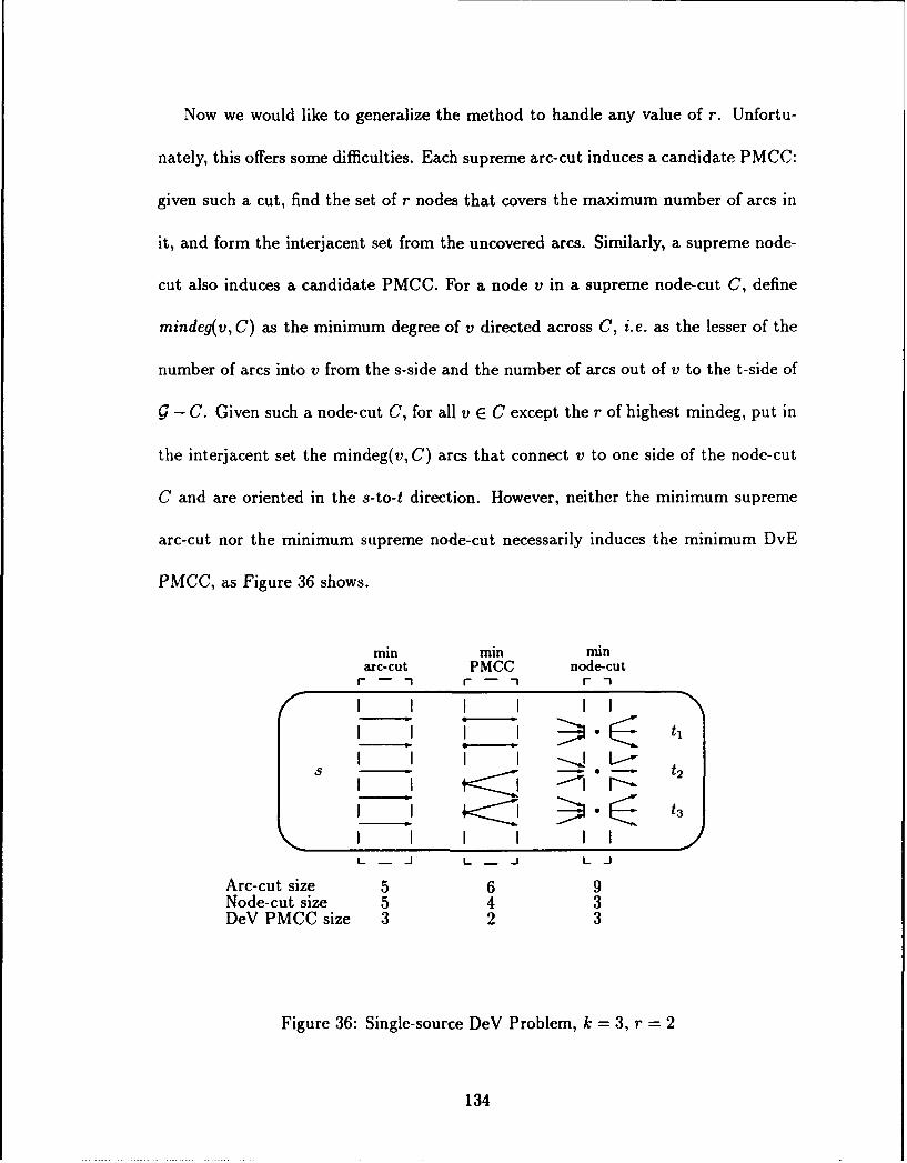
Now we would like to generalize the method to handle any value of r. Unfortu-

nately, this offers some difficulties. Each supreme arc-cut induces a candidate PMCC:

given such a cut, find the set of r nodes that covers the maximum number of arcs in

it, and form the interjacent set from the uncovered arcs. Similarly, a supreme node-

cut also induces a candidate PMCC. For a node v in a supreme node-cut C, define

mindeg(v, C) as the minimum degree of v directed across C, i.e. as the lesser of the

number of arcs into v from the s-side and the number of arcs out of v to the t-side of

9 - C. Given such a node-cut C, for all v E C except the r of highest mindeg, put in

the interjacent set the mindeg(v, C) arcs that connect v to one side of the node-cut

C and are oriented in the s-to-t direction. However, neither the minimum supreme

arc-cut nor the minimum supreme node-cut necessarily induces the minimum DyE

PMCC, as Figure 36 shows.

min min minarc-cut PMCC node-cut

r - - r -• r I

I J I I J

Arc-cut size 5 6 9Node-cut size 5 4 3DeV PMCC size 3 2 3

Figure 36: Single-source DeV Problem, k = 3, r =2

134

To find the optimal interjacent set for r > 2, we will need the following two

propositions. The first is the equivalent of Lemma 13 for the DeE case.

Proposition 23 Suppose J is an optimal partial multicommodity directed cut in a

single-source, arc-cut, node-disjoint problem. Then all s-ti paths in ! - J = TI can be

partitioned into two sets as follows. One set consists of paths to a member of a set of

sinks Q, the other set is covered by a set of nodes P, and IQI + IPI = r. Furthermore,

there are no such sets Q' and P' that cover all paths and have IQ'I + IP'I < r.

Proof: Let 1?' be the union of all s-ti paths in 1?, plus t' and the terminal arcs

tit', and with all nodes (except the terminals and t') split into an in-node and an

out-node. Put capacity 1 on the node arcs and terminal arcs, let other arcs have

unlimited capacity, and find a feasible maximum s-t' flow. The total flow can be no

more than r, so the minimum cut is no more than r. Neither can the flow be less than

r: if it is, one arc can be deleted from J and added to R and result in a maximum

flow of no more than r in 1V', contradicting the optimality of J. Then the minimum

cut in 1V' must be exactly r, and it must correspond to a set Q of sinks plus a set P

of nodes, where P and Q together cover all paths and IQI + IPI = r. Furthermore, if

there were a set of sinks Q' and a set of nodes P' with IQ'I + JP'1 < r that covered all

s-ti paths in 1?, then the maximum flow in VI' would also have to be less than r. M

Proposition 24 Given J, P, and Q as defined in Proposition 23, J is a minimum

arc-cut between s and T - Q in (G - P) - Q.

Proof: Suppose C* is a minimum arc-cut as described and IC*I < jJI. Then in

- C* any s-ti path must either go to a member of Q or pass through a member

135

of P. There can be no more than IPI + IQI = r node-disjoint such paths to different

sinks. Therefore C* is a feasible PMCC, and JClJ __ JJJ, a contradiction. 0

From Proposition 24, it is clear that for some set N consisting of r nodes in

(excluding s, but possibly including sinks), the optimal PMCC J is the minimum

supreme arc-cut in -N. This means we can find J by evaluating (n) minimum

cut problems (n = JVi). This involves O(n'rr) or 0(n0`7) work, where a minimum

cut can be found in 0(77) work, and is polynomial if n - r or r is bounded.

Though it will not change the bound, some of the evaluations may be deleted by

considering the non-sink nodes in order of decreasing lesser degree. For any candidate

PMCC J and its sets P and Q as defined in Proposition 23, a supreme cut is formed

by J plus the in-arcs on the members of Q plus either the in-arcs or the out-arcs

of each member of P. If we define the lesser degree of a sink as its in-degree and

lesdeg(v) as the lesser degree of v, the cardinality of this supreme cut is

1JI + E lesdeg(v) + E lesdeg(v) = Csup (71)vEP vEQ

If the smallest supreme cut in g is of size c, we can conclude that

Csup > c (72)

Once we have a candidate PMCC of size j, to have hIJ < J we must have

j > csup- Z iesdeg(v) > c- E lesdeg(v) (73)vEPUQ vE PUQ

E lesdeg(v) > c-j (74)vEPUQ

Thus we only need to consider sets P and Q whose total lesser degree is at least

c-j + 1.

136

8.5 The Cross-case DvE

This is the problem of removing the smallest number of nodes from a digraph so

that there are no more than r arc-disjoint paths left between the source and distinct

members of the set of sinks. This might represent a pipeline network in which capacity

was limited by the pipes, but questions are being asked about the consequences of

failures at pumping stations at the nodes. Without loss of generality we can assume

that s has zero in-degree, the sinks have positive in-degree, and all terminals (except

possibly the sinks) have positive out-degree.

Let us first consider the case of r = 1. Candidate PMCCs can be found by

finding the minimum node-cuts between s and each of the k sets of all terminals but

one. Suppose the smallest of these is of cardinality j. The only possibility for a

smaller interjacent set is that there might be a full multicommodity node-cut also of

cardinality j that included a node that was either the head of exactly one arc from

the s-side of the cut or the tail of exactly one arc to the t-side of the cut. Let us

call such a node a mindeg-J node in relation to a given node-cut (see Figure 37).

If a mindeg-1 node is deleted from an FMCC, the remaining graph 1Z can contain

only one arc-disjoint path from s to any ti. This PMCC would then be optimal, at

cardinality j - 1.

A cut containing a mindeg-1 node, if it exists, can be found with one more min-

imum cut evaluation in the following way. Reformulate the problem into an arc-cut

problem in the standard way by splitting each node into an in-node and an out-node

connected by a weight-i node arc, but weight all the other arcs at 1 - - (where

137

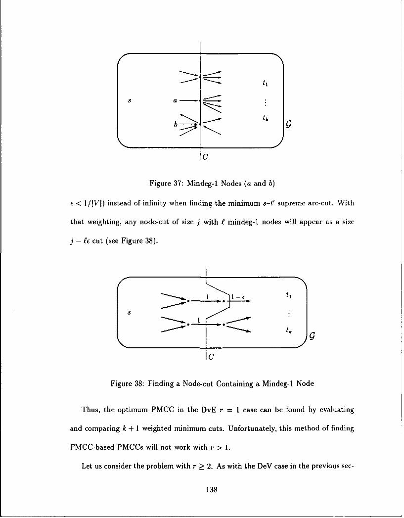
S a

tk

C

Figure 37: Mindeg-1 Nodes (a and b)

f < 1/[V[) instead of infinity when finding the minimum s-t' supreme arc-cut. With

that weighting, any node-cut of size j with I mindeg-1 nodes will appear as a size

j - eE cut (see Figure 38).

E tk

Figure 38: Finding a Node-cut Containing a Mindeg-1 Node

Thus, the optimum PMCC in the DyE r = 1 case can be found by evaluating

and comparing k + 1 weighted minimum cuts. Unfortunately, this method of finding

FMCC-based PMCCs will not work with r > 1.

Let us consider the problem with r > 2. As with the DeV case in the previous sec-

138

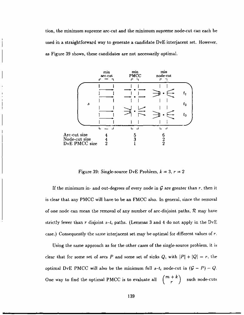
tion, the minimum supreme arc-cut and the minimum supreme node-cut can each be

used in a straightforward way to generate a candidate DvE interjacent set. However.,

as Figure 39 shows, these candidates are not necessarily optimal.

min min minarc-cut PMCC node-cut

I -I f- "1 F -r - I I I I

S t2I1 ~ _IL I Is t3--.I <FI

III I IL • J L .J L .

Arc-cut size 4 5 6Node-cut size 4 3 2DvE PMCC size 2 1 2

Figure 39: Single-source DyE Problem, k = 3, r = 2

If the minimum in- and out-degrees of every node in g are greater than r, then it

is clear that any PMCC will have to be an FMCC also. In general, since the removal

of one node can mean the removal of any number of arc-disjoint paths, 1? may have

strictly fewer than r disjoint s-ti paths. (Lemmas 3 and 4 do not apply in the DyE

case.) Consequently the same interjacent set may be optimal for different values of r.

Using the same approach as for the other cases of the single-source problem, it is

clear that for some set of arcs P and some set of sinks Q, with JP1 + tQI = r, the

optimal DyE PMCC will also be the minimum full s-ti node-cut in (!9 - P) - Q.

One way to find the optimal PMCC is to evaluate all m + k) such node-cuts

139

(m = IEI). This method results in a combinatorial explosion unless m + k, r, or

rn + k - r is bounded.

8.6 Undirected Nearly T-Planar Graphs (UeEP)

If a single-source undirected multicommodity flow graph 9 is planar and has all its

sinks on the boundary, call it sink-planar. This section will develop a polynomially-

bounded algorithm for sink-planar graphs.

Without loss of generality, number the sinks from tj to tk clockwise around !.

Form W' from ! by adding the super-sink t' and the k terminal edges tit' (see Fig-

ure 40; note that g' is planar.) From Lemma 14, we know that the smallest PMCC J

corresponds to the smallest s-t' cut C' that contains no more than r terminal edges,

and that J is found by deleting from C' any r edges, to include any terminal edges

in C', so that IJI = IC'I - r. The following characerizes C', assuming it contains

terminal edges.

C' must be a minimal cut in !', corresponding to a circuit in the geometric-dual

of g'. It will consist of alternating sets of edges A, T1, A2, T2,..., At, Tt (I < k/2),

where each Ai separates from the rest of Q a set of terminals from some t. clockwise

to t b (in Figure 40, A, separates t3 to ts), and each Ti consists of a set of consecutive

terminal arcs (in Figure 40, T, consists of t6 t' through t9 t'). The sets of terminals

associated with each of the Ai and Ti form a partition of the set of sinks T - {s}. As

in previous chapters, let us use the conventions that t, E ti.±k, [ti, tj] means the set of

terminals from ti clockwise around 9 through tj, and [ti, ti-] =

140

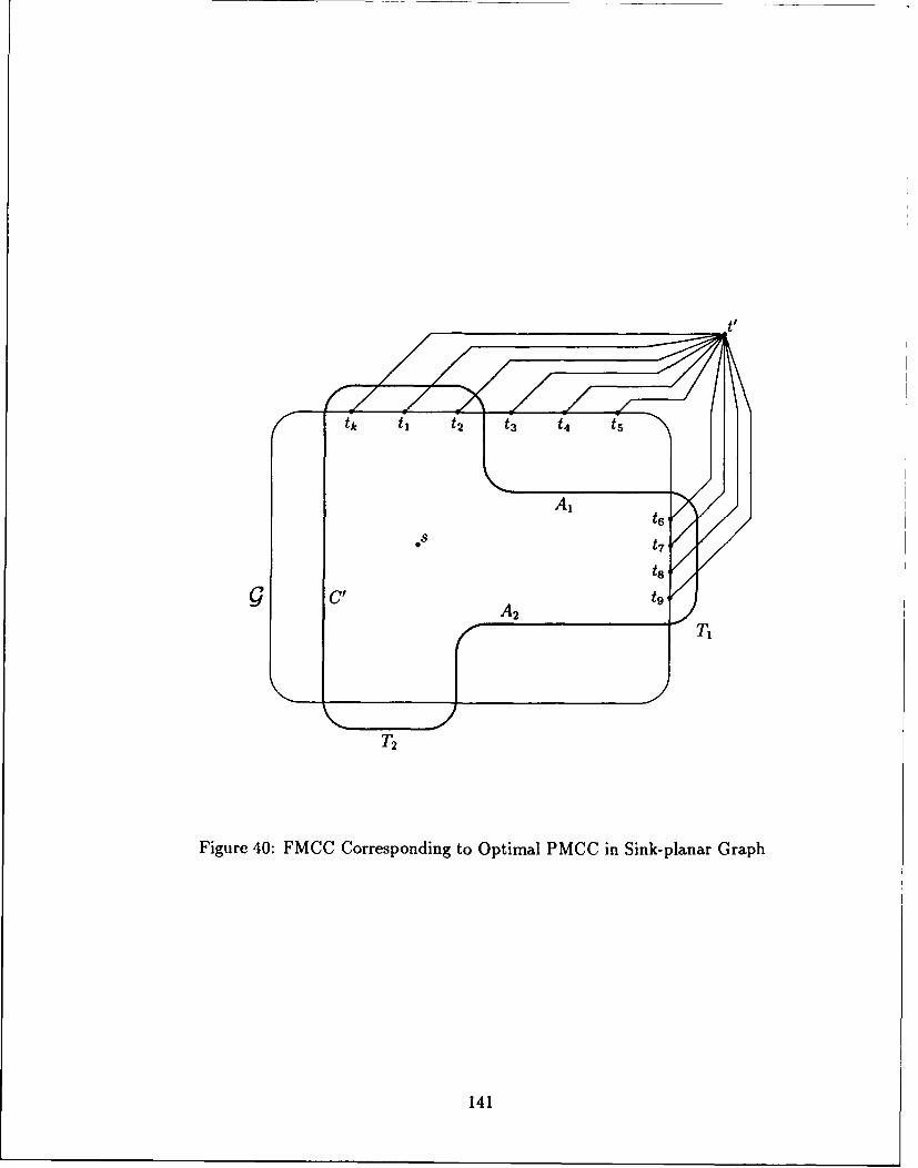
tk t I t2 t3 t t5

A, tt7

t8

SA2 t9 F

T22

Figure 40: FMCC Corresponding to Optimal PMCC in Sink-planar Graph

141

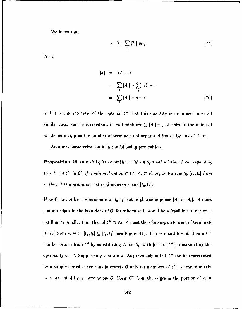
We know that

r 75•'llq T,

A I0o,

IJI IC"I -

-= • jaI + IT, 1 - ,r* S

- IA,I +q - r (76)i

an1dt, t is ch1itnterristic of the optimhal C' that, this qwutt.tity is minimized over all

mitIilar (cuts. Siunce r is cOn|titant, (' will minimize IrA, I + q, the, size of the1 iiuioti of

all the cutm A.l pluN the h unulbr of te'rminals not, nepartAterd from , by a.ny of them.

A iother hcltra•lterizatiou iN in the following proposition.

Propositiou 25 In a .Nink.planar probilrvn with an optimal solution J corlr.spoutind

to ,4 t' cut (' in V', if a ininitial cut A, C C', A, C E, qrparatrc. rcactly [I,,, t•] from

,/ hri it is a minimum cut in J brtwriea s anid [t,,, t1.

Proof: Let A be the miniiimum .4 [t , 4] cut in V, mid( suppose JA <, IA,[. A |mumt.

cou)itail edgem ini the boundary of 0, for otherwiNe it, would be, a feaNible ,4 t' (lit with

Cardintlity Mmaller thati that of C' : A,. A tmunt therefore separate a itet of terminiNhis

It., tf] I'romi ,., with (t1,, tb] gt,,, t]d (Nee Figure 41I). If a = c and b = d, th.ii it C"

('11,1 hhe uorined fromt (7' by NstbNtituting A for A,, with I(C"I < 1( '], contradiicting the

olptiiltlity of ('. Suppowe a 0 1 or b • d. Am previouNly noted, C" can be repremented

by i simple close•e curve that, intermectm Q only oti IneinberN of (C'. A can Nimilarly

be re,)reuette(d by a ctirve acrosa s, l.orm C" from the edges in the portion of A in

142

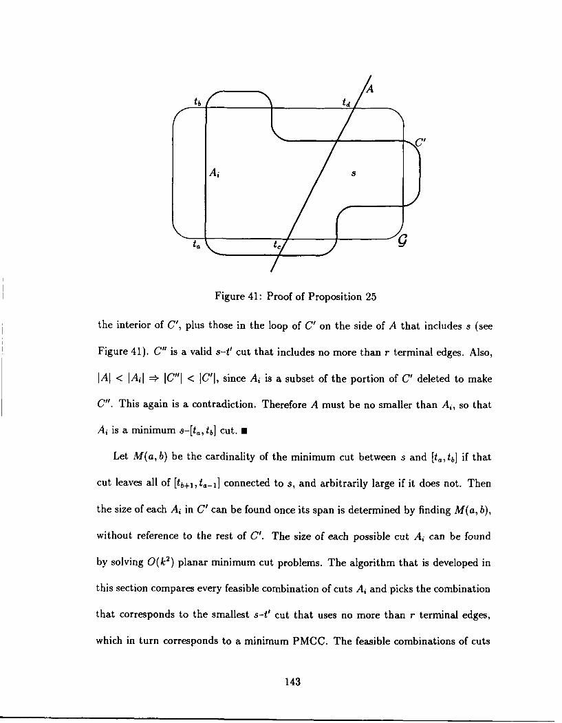
tb td- /At

A S

Figure 41: Proof of Proposition 25

the interior of C', plus those in the loop of C' on the side of A that includes s (see

Figure 41). C" is a valid s-t' cut that includes no more than r terminal edges. Also,

IAI < IAI =€" IC"I < IC'I, since A, is a subset of the portion of C' deleted to make

C". This again is a contradiction. Therefore A must be no smaller than Ai, so that

Ai is a minimum s-[ta, tb] cut. U

Let M(a, b) be the cardinality of the minimum cut between s and [ta, tb] if that

cut leaves all of [tb+1, t.- 1 ] connected to s, and arbitrarily large if it does not. Then

the size of each Ai in C' can be found once its span is determined by finding M(a, b),

without reference to the rest of C'. The size of each possible cut A, can be found

by solving 0(k 2 ) planar minimum cut problems. The algorithm that is developed in

this section compares every feasible combination of cuts Ai and picks the combination

that corresponds to the smallest s-t' cut that uses no more than r terminal edges,

which in turn corresponds to a minimum PMCC. The feasible combinations of cuts

143

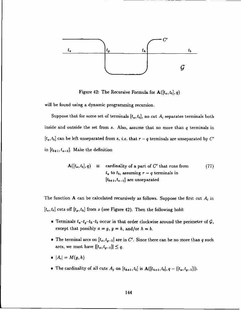
- C1

t9 th _ tb

L-- G

Figure 42: The Recursive Formula for A([ta, tb], q)

will be found using a dynamic programming recursion.

Suppose that for some set of terminals [ta, tb], no cut Ai separates terminals both

inside and outside the set from s. Also, assume that no more than q terminals in

[t,, tb] can be left unseparated from s, i.e. that r - q terminals are unseparated by C'

in [tb+l, t,-I]. Make the definition

A([ta, tb], q) cardinality of a part of C' that runs from (77)ta to tb, assuming r - q terminals in

[tb+l, ta,-1] are unseparated

The function A can be calculated recursively as follows. Suppose the first cut A, in

[ta, tb] cuts off [tg, th] from s (see Figure 42). Then the following hold:

"* Terminals ta-tg-th-tb occur in that order clockwise around the perimeter of g,except that possibly a = g, g = h, and/or h = b.

"* The terminal arcs on [ti, tg-l] are in C'. Since there can be no more than q sucharcs, we must have I[ta, ty-]I < q.

"• Ia I = M(g,h)

"* The cardinality of all cuts Aj on [th+1, tb] is A([th+l, tb], q - Ita, tg_1]lD-

144

So we have following recursion for A:

A([t Itb],q) = min D[a,g) + min {M(g,h) + A([th+1,tb],q - Dia4))} (78)*9EQg tjhE1t,,tb]J

where

Dra,9) = 11t. ,t9_1]l

Q = {tg : tg E [t.,tb+,I DOi.,g) < q}

and min over a null set is taken to be zero. The recursion can be initiated with

A(0,q) = 0 for alla, q>0 (79)

The function A can be used to find C' if the latter includes at least one terminal

edge. If C' includes tit', then

IC'- = A([ti+,, ti_.], r - 1) (80)

If C' includes no terminal edges, then it is the minimum supreme cut. In either case,

r edges (including any terminal edges) may be deleted from C' to find an optimal

PMCC. Combining both possibilities, we get the following algorithm.

145

Algorithm 13 (Single-source Sink-planar UeEP PMCC)

input: g' and r for a single-source sink-planar UeEP PMCC problem

output: cardinality of an optimal interjacent set J in

begin

compute c, = size of minimum supreme cut

for every set [t., tb] of cardinality less than k

compute M(a, b)

for q = 0,...,r

set A(O,q) = 0

fori= 1,...,k-1

for every set [ta, tb] of cardinality ifor q = 0,...,r

compute A([ta,t 6 l, q) using (78)

return min Co mmin {A([tj+,,tjl,r - 1) - r

end

The complexity is O(k 2 - + r2 k 3 ), where -f is the complexity of finding a planar min-

imum cut. We conclude with the following theorem.

Theorem 7 The single-source sink-planar partial multicommodity edge-cut problem

with edge-disjoint remaining paths is polynomially bounded.

Proof: Algorithm 1.i provides a polynomia, procedure for this problem. m

146

9 CONCLUSIONS AND FUTURE WORK

This chapter summarizes the work and points out some likely directions for fu-

ture investigations. The results in Chapter 4 showed that the general MCC problem

was intractable, so investigation was focused on restricted special cases that offered

promise. Following are discussions of the four major lines of research on multicom-

modity cuts: full edge-cuts, partial edge-cuts, and vertex-cuts, all in planar graphs;

and the single-source partia! cut problem in general graphs.

In the area of full multicommodity cuts in T-planar graphs the research seems to

be most nearly complete. There are polynomial algorithms for the weighted problem

with fixed k (Aig. 2) and in non-crossing graphs with varying k (Alg. 4), and in view

of Proposition 10 there is little more to be expected, except perhaps in more restricted

cases. It is perhaps something of a disappointment that the T-planar FMCC problem

should turn out to be NP-complete even in classes of graphs as restricted as grids

and weighted trees. Its status in unweighted trees would be interesting to know, but

this is still open. If the terminals are not restricted to the boundary the problem can

certainly be no easier than the T-planar version, so polynomial algorithms for fixed

k are what is to be hoped for. Algorithm 3 was developed for the k = 3 case. It

would be good to find a unifying treatment that would work for any fixed k in general

planar graphs.

Prospects for efficient algorithms for partial multicommodity edge-cuts are se-

verely limited by the intractability of the closely associated full multicommodity cut

and disjoint paths problems. This work had some success with the PMCC problem

in T-planar non-crossing graphs for r = k - 1 (Aig. 6), r = k - 2 (Alg. 7), and r = 1

(AIg. 8). It would be good to have a unifying treatment that would close the gap

(k-3 > r > 2). It seems clear that what is needed is an account of the characteristics

of T-planar q-disjoint-path graphs, i.e. multicommodity flow graphs in which only q

disjoint si-ti paths can be found. Also, only the unweighted PMCC problem was

investigated. The corresponding weighted problem is still open.

Chapter 7 showed that some of the major results for multicommodity edge-cuts

can be extended readily to vertex-cuts. It seems likely that efforts to extend the

remaining results (full three-commodity cuts in general planar graphs; partial cuts in

T-planar graphs with r < k - 2) would be rewarded.

The single-source problem turned out to be relatively easy, and it was handled

successfully in the greatest variety of cases. However, some interesting open questions

remain. The question of greatest theoretical interest is whether the general problem

is NP-complete for arbitrary k and r; it was shown to be polynomial for r or k - r

bounded (Proposition 22). Also, the cross-cases DyE and DeV were handled satis-

factorily only for k = 1, and the undirected cross-cases were not addressed. The

weighted single-source problem remains open. Finally, it would be interesting to see

if the specialized algorithm for the undirected PMCC problem in sink-planar graphs

(Alg. 13) could be extended to directed graphs.

148

Except for single-source problems, this research concentrated on multicommodity

cuts in undirected graphs. It would be interesting to know if these or similar methods

could be used to find full or partial multicommodity cuts in directed planar or T-

planar graphs.

149

REFERENCES

[1] Aneja, Y. P. and R. R. Vemuganti. 1977. A Row-generation Scheme for Findinga Multi-commodity Minimum Disconnecting Set. Management Science, 23, 652-659.

[2] Assad, A. A. 1978. Multicommodity Network Flows-A Survey. Networks, 8,37-91.

(31 Becker, M. and K. Mehlhorn. 1986. Algorithms for Routing in Planar Graphs.Acta Informatica, 23, 163-176.

[4] Bellmore, M., H. J. Greenberg, and J. J. Jarvis. 1970. Multi-commodity Discon-necting Sets. Management Science, 16, B427-B433.

[5] Dahlhaus, E., D. S. Johnson, C. H. Papadimitriou, P. D. Seymour, and M. Yan-nakakis. 1992. The Complexity of Multiway Cuts. Proceedings of the Twenty-fourth Annual ACM Symposium of the Theory of Computing (New York: ACMPress), 241-251.

[6] Ding, G., A. Schrijver, and P. D. Seymour. 1992. Disjoint Paths in a PlanarGraph-A General Theorem. SIAM Journal on Discrete Mathematics, 5, 112-116.

[71 Erickson, R. E., C. L. Monma, and A. F. Veinott. 1987. Send and Split Methodfor Minimum-concave-cost Network Flows. Mathematics of Operations Research,12, 634-664.

[8) Evans, J. R. and J. J. Jarvis. 1979. Network Topology and Integral Multicom-modity Flow Problems. Networks, 8, 107-119.

[91 Even, S., A. Itai, and A. Shamir. 1976. On the Complexity of Timetable andMulticommodity Flow Problems. SIAM Journal on Computing, 5, 691-703.

[101 Floyd, R. W. Algorithm 97: Shortest Path. Communications of the ACM, 5,345.

[11] Ford, L. R. and D. R. Fulkerson. 1956. Maximal Flow through a Network. Cana-dian Journal of Mathematics, 8, 399-404.

[12] Fortune, S., J. Hopcroft, and J. Wyllie. 1980. The Directed Subgraph Homeo-morphism Problem. Journal of Theoretical Computer Science, 10, 111-121.

[13] Frank, A. 1985. Edge-disjoint Paths in Planar Graphs. Journal of CombifiatorialTheory, Series B, 39, 164-178.

150

[14] Frank, A. 1990a. On Disjoint Homutopic Paths in the Plane. Polyhedral Combi-natorics, W. Cook and P. D. Seymour, eds. (Morristown, NJ: American Mathe-matical Society), 163-170.

[15] Frank, A. 1990b. Packing Paths, Circuits, and Cuts-A Survey. Paths, Flowsand VLSI-layout, B. Korte, L. Loviisz, H. J. Pramel, and A. Schrijver, eds. (NewYork: Springer-Verlag), 47-100.

[16] Frank, A. 1990c. Packing Paths in Planar Graphs. Combinatorica, 10, 325-331.

[17] Frank, A. and A. Schrijver. 19.J. Vertex-disjoint Simple Paths of Given Homo-topy in a Planar Graph. Polyhedral Combinatorics, W. Cook and P. D. Seymour.eds. (Morristown, NJ: American Mathematical Society), 139-161.

[18] Frederickson, G. N. 1987. Fast Algorithms for Shortest Paths in Planar Graphs,with Applications. SIAM Journal on Computing, 16, 1004-1022.

[19] Garey, M. R., and D. S. Johnson. 1979. Computers and Intractability: A Guideto the Theory of NP-Completeness (New York: W. H. Freeman and Company).

[20] Garey, M. R., D. S. Johnson, and L. Jtockmeyer. 1976. Some SimplifiedNP-Complete Graph Problems. Theoretical Computer Science, 1, 237-267.

[21] Hassin, R. 1984. On Multicommodity Flows in Planar Graphs. Networks, 14,225-235.

[22] Hu, T. C. 1963. Multi-commodity Network Flows. Operations Research, 11, 344-360.

[23] Jarvis, J. J. and J. B. Tindall. 1972. Minimal Disconnecting Sets in DirectedMulti-commodity Networks. Naval Research Logistics Quarterly, 19, 681-690.

[24] Kennington, J. L. 1978. A Survey of Linear Cost Multi-commodity NetworkFlows Operationq Research, 26, 209-236.

[25] Kohn, M. C. and R. D. 1 'mieux. 1991. Identification of Regulatory Propertiesof Metabolic Networks by Graph Theoretical Modeling. Journal of TheoreticalBiology, 150, 3-25.

[26] Lai, T.-H. and A. Sprague. 1987. On the Routability of a Convex Grid. Journalof Algorithms, 8, 372-384.

[27] Larman, D. G. and P. Mani. 1970. On the Existence of Certain Configurationswithin Graphs and the 1-Skeleton of Polytopes. Proceedings of the London Math-ematical Society, 20, 144-160.

[28] Matsumoto, K., T. Nishizeki, and N. Saito. 1985. An Efficient Algorithm forFinding Multicommodity Flows in Planar Networks. SIAM Journal on Comput-ing, 14, 289-302.

151

[29] Mehlhorn, K. and F. P. Preparata. 1986. Routing through a Rectangle. Journalof the A CM, 33, 60-85.

[30] Middendorf, M. and F. Pfeiffer. 1990. On the Complexity of the Disjoint PathsProblem. Polyhedral Combinatorics, W. Cook and P. D. Seymour, eds. (Morris-town, NJ: American Mathematical Society), 171-178.

[311 Okamura, H. 1983. Multicommodity Flows in Graphs. Discrete Applied Mathe-matics, 6, 55-62.

[32] Okamura, H. and P. D. Seymour. 1981. Multicommodity Flows in Planar Graphs.Journal of Combinatorial Theory, Series B, 31, 75-81.

[33] Nagamochi, H. and T. Ibaraki. 1989. On Max-flow Min-cut and Integral FlowProperties in Directed Networks. Information Processing Letters, 31, 279-285.

[34] Perl, M. and Y. Shiloach. 1978. Finding Two Disjoint Paths between Two Pairsof Vertices in a Graph. Journal of the ACM, 25, 1-9.

[35] Provan, J. S. 1983. A Polynomial Algorithm for the Steiner Tree Problem onTerminal-planar Graphs. Technical Report 83/10, Department of Operations Re-search, University of North Carolina, Chapel Hill, NC.

[36] Provan, J. S. 1988. Convexity and the Steiner Tree Problem. Netnoorks, 18, 55-72.

[37] Robertson, N. and P. D. Seymour. 1985. Disjoint Paths-A Survery. SIAM Jour-nal on Algebraic and Discrete Methods, 6, 300-305.

[38] Robertson, N. and P. D. Seymour. 1986. Graph Minors VI: Disjoint Paths acrossa Disc. Journal of Combinatorial Theory, Series B, 41, 115-138.

[39] Robertson, N. and P. D. Seymour. 1988. Graph Minors VII: Disjoint Paths on aSurface. Journal of Combinatorial Theory, Series B, 45, 212-254.

[40] Rothschild, B. and A. Whinston. 1966. On Two Commodity Network Flows.Operations Research, 14, 377-387.

[41] Sakarovitch, M. 1973. Two Commodity Network Flows and Linear Programming.Mathematical Programming, 4, 1-20.

[42] Schrijver, A. 1983. Min-max Results in Combinatorial Optimization. Mathemat-ical Programming, A. Bachem, M. Grttschel, and B. Korte, eds. (New York:Springer-Verlag), 439-500.

[43] Schrijver, A. 1989. The Klein Bottle and Multicommodity Flows. Combinatorica,9, 375-384.

[44] Schrijver, A. 1990. Homotopic Routing Methods. Paths, Flows, and VLSI-layout,B. Korte, L. Lovisz, H. J. Pr~mel, and A. Schrijver, eds. (New York: Springer-Verlag), 329-371.

152

[45] Schrijver, A. 1991. Short Proofs on Multicommodity Flows and Cuts. Journal ofCombinatorial Theory, Series B, 53, 32-39.

[46] Schrijver, A. No date. Multicommodity Flows and Disjoint Paths. UnpublishedMS.

[47] Seb6, A. 1990. The Cographic Multiflow Problem: An Epilogue. Polyhedral Com-binatorics, W. Cook and P.D. Seymour, eds. (Morristown, NJ: American Math-ematical Society), 203-234.

[48] Seymour, P. D. 1980a. Disjoint Paths in Graphs. Discrete Mathematics, 29,293-309.

[49] Seymour, P. D. 1980b. Four-terminus Flows. Networks, 10, 79-86.

[50] Seymour, P.D. 1981a. Matroids and Multicommodity Flows. European Journalof Combinatorics, 2, 257-290.

[51] Seymour, P. D. 1981b. On Odd Cuts and Plane Multicommodity Flows. Pro-ceedings of the London Mathematical Society, Series 3, 42, 178-192.

[52] Shiloach, Y. 1980. A Polynomial Solution to the Undirected Two Paths Problem.Journal of the ACM, 27, 445-456.

[53] Suzuki, H., A. Ishiguro, and T. Nishizeki. 1990. Edge-disjoint Paths in a GridBounded by Two Nested Rectangles. Discrete Applied Mathematics, 27, 157-178.

[54] Thomassen, C. 1985. The 2-Linkage Problem for Acyclic Digraphs. DiscreteMathematics, 55, 73-87.

[55] Watkins, M. E. 1968. On the Existence of Certain Disjoint Arcs in Graphs. DukeMathematical Journal, 35, 231-246.

[56] Wilson, R. J. 1985. Introduction to Graph Theory, 3rd ed. (London: LongmanScientific & Technical).

153