Looking for cosmic ray sources: a study of gamma-ray ... Looking for cosmic ray sources: ......
112
UNIVERSIT ` A DEGLI STUDI DI PADOVA Facolt ` a di Scienze Matematiche Fisiche e Naturali Corso di Laurea Specialistica in Fisica Tesi di Laurea Looking for cosmic ray sources: a study of gamma-ray emission from molecular clouds with the GLAST LAT telescope. Relatore: prof. Giovanni Busetto Correlatore: dott. Riccardo Rando Laureando: Luigi Tibaldo Anno Accademico 2006/2007
Transcript of Looking for cosmic ray sources: a study of gamma-ray ... Looking for cosmic ray sources: ......

UNIVERSITA DEGLI STUDI DI PADOVAFacolta di Scienze Matematiche Fisiche e Naturali
Corso di Laurea Specialistica in Fisica
Tesi di Laurea
Looking for cosmic ray sources:a study of gamma-ray emission from molecular clouds
with the GLAST LAT telescope.
Relatore: prof. Giovanni Busetto
Correlatore: dott. Riccardo Rando
Laureando: Luigi Tibaldo
Anno Accademico 2006/2007


The changing of bodies into light,and light into bodies,
is very comformable to the course of Nature,which seems delighted with transmutations.
Isaac Newton, Optics, 1704.


i
Contents
Abstract 1
Prefazione 2
1 The sky in gamma rays 31.1 Gamma ray production and detection . . . . . . . . . . . . . . . . . . . . 3
1.1.1 Production processes . . . . . . . . . . . . . . . . . . . . . . . . . 31.1.2 Gamma ray propagation . . . . . . . . . . . . . . . . . . . . . . . 51.1.3 Detection techniques . . . . . . . . . . . . . . . . . . . . . . . . . 6
1.2 Gamma ray telescopes . . . . . . . . . . . . . . . . . . . . . . . . . . . . 71.2.1 Imaging via collimators . . . . . . . . . . . . . . . . . . . . . . . . 71.2.2 Imaging via modulation techniques . . . . . . . . . . . . . . . . . 81.2.3 Compton telescopes . . . . . . . . . . . . . . . . . . . . . . . . . . 91.2.4 Pair-tracking telescopes . . . . . . . . . . . . . . . . . . . . . . . 111.2.5 Cherenkov telescopes . . . . . . . . . . . . . . . . . . . . . . . . . 121.2.6 GRB instruments . . . . . . . . . . . . . . . . . . . . . . . . . . . 131.2.7 The GLAST mission . . . . . . . . . . . . . . . . . . . . . . . . . 14
1.3 Gamma ray sources . . . . . . . . . . . . . . . . . . . . . . . . . . . . . . 151.3.1 Solar system objects . . . . . . . . . . . . . . . . . . . . . . . . . 151.3.2 Pulsars . . . . . . . . . . . . . . . . . . . . . . . . . . . . . . . . . 161.3.3 Supernova remnants . . . . . . . . . . . . . . . . . . . . . . . . . 171.3.4 X-ray binaries . . . . . . . . . . . . . . . . . . . . . . . . . . . . . 181.3.5 Active galactic nuclei . . . . . . . . . . . . . . . . . . . . . . . . . 191.3.6 Gamma ray bursts . . . . . . . . . . . . . . . . . . . . . . . . . . 201.3.7 Dark matter . . . . . . . . . . . . . . . . . . . . . . . . . . . . . . 211.3.8 Diffuse gamma rays . . . . . . . . . . . . . . . . . . . . . . . . . . 21
2 Diffuse galactic gamma rays: a cosmic ray tracer 232.1 Cosmic ray physics . . . . . . . . . . . . . . . . . . . . . . . . . . . . . . 23
2.1.1 The Sun as a CR source and modulator . . . . . . . . . . . . . . 232.1.2 Extrasolar CRs: direct observations . . . . . . . . . . . . . . . . . 242.1.3 CR interactions in the interstellar medium . . . . . . . . . . . . . 27
2.2 GALPROP models . . . . . . . . . . . . . . . . . . . . . . . . . . . . . . 292.2.1 The GALPROP code . . . . . . . . . . . . . . . . . . . . . . . . . 302.2.2 Constraints from CR direct observations . . . . . . . . . . . . . . 322.2.3 Diffuse galactic gamma rays . . . . . . . . . . . . . . . . . . . . . 34
2.3 Diffuse gamma rays from molecular clouds . . . . . . . . . . . . . . . . . 37
ii Contents
2.3.1 The emission model . . . . . . . . . . . . . . . . . . . . . . . . . . 372.3.2 X-ratio calibration . . . . . . . . . . . . . . . . . . . . . . . . . . 40
3 The Large Area Telescope 413.1 The LAT instrument . . . . . . . . . . . . . . . . . . . . . . . . . . . . . 41
3.1.1 The Anticoincidence Detector . . . . . . . . . . . . . . . . . . . . 413.1.2 The Tracker . . . . . . . . . . . . . . . . . . . . . . . . . . . . . . 433.1.3 The Calorimeter . . . . . . . . . . . . . . . . . . . . . . . . . . . 443.1.4 Data Acquisition and triggering . . . . . . . . . . . . . . . . . . . 453.1.5 Track and energy release reconstruction . . . . . . . . . . . . . . . 46
3.2 The Instrument Response Functions . . . . . . . . . . . . . . . . . . . . . 473.2.1 IRF definition . . . . . . . . . . . . . . . . . . . . . . . . . . . . . 473.2.2 IRF development: the simulation tools . . . . . . . . . . . . . . . 483.2.3 DC2 IRFs . . . . . . . . . . . . . . . . . . . . . . . . . . . . . . . 49
3.3 The extended maximum Likelihood analysis for LAT data . . . . . . . . 513.3.1 The extended maximum Likelihood method . . . . . . . . . . . . 513.3.2 The unbinned analysis . . . . . . . . . . . . . . . . . . . . . . . . 533.3.3 The binned analysis . . . . . . . . . . . . . . . . . . . . . . . . . . 54
4 A model for analysis of gamma-ray emission from molecular clouds 554.1 The simulation . . . . . . . . . . . . . . . . . . . . . . . . . . . . . . . . 55
4.1.1 The GALPROP model . . . . . . . . . . . . . . . . . . . . . . . . 554.1.2 The LAT observation simulation . . . . . . . . . . . . . . . . . . . 56
4.2 Tests at high energies . . . . . . . . . . . . . . . . . . . . . . . . . . . . . 574.2.1 The spectral model . . . . . . . . . . . . . . . . . . . . . . . . . . 584.2.2 The spatial distribution of IC emission . . . . . . . . . . . . . . . 634.2.3 Spectral behavior of the gas-related components . . . . . . . . . . 66
4.3 Extension at low energies . . . . . . . . . . . . . . . . . . . . . . . . . . . 674.3.1 The multi-energy range analysis . . . . . . . . . . . . . . . . . . . 674.3.2 Analysis between 1 GeV and 32 GeV . . . . . . . . . . . . . . . . 694.3.3 Analysis between 562 MeV and 1 GeV . . . . . . . . . . . . . . . 70
4.4 Comparison with the model . . . . . . . . . . . . . . . . . . . . . . . . . 714.4.1 Systematic errors . . . . . . . . . . . . . . . . . . . . . . . . . . . 714.4.2 Systematics evaluation . . . . . . . . . . . . . . . . . . . . . . . . 73
5 Analysis of diffuse emission in Monoceros on simulated LAT data 755.1 The EGRET sky model . . . . . . . . . . . . . . . . . . . . . . . . . . . 75
5.1.1 EGRET sources . . . . . . . . . . . . . . . . . . . . . . . . . . . . 755.1.2 Point sources subtraction . . . . . . . . . . . . . . . . . . . . . . . 785.1.3 Analysis of diffuse emission . . . . . . . . . . . . . . . . . . . . . 79
5.2 The DC2 sky model . . . . . . . . . . . . . . . . . . . . . . . . . . . . . . 835.2.1 DC2 sources . . . . . . . . . . . . . . . . . . . . . . . . . . . . . . 835.2.2 Diffuse emission and point sources . . . . . . . . . . . . . . . . . . 83
5.3 Comparison with the model . . . . . . . . . . . . . . . . . . . . . . . . . 875.3.1 The reconstructed spectrum . . . . . . . . . . . . . . . . . . . . . 875.3.2 X-ratio calibration . . . . . . . . . . . . . . . . . . . . . . . . . . 90
5.4 Conclusions . . . . . . . . . . . . . . . . . . . . . . . . . . . . . . . . . . 92

Contents iii
A Theoretical elements about cosmic ray propagation and acceleration 94
B Abbreviations 97
Bibliography 99
Acknowledgments 103
Ringraziamenti 104

1
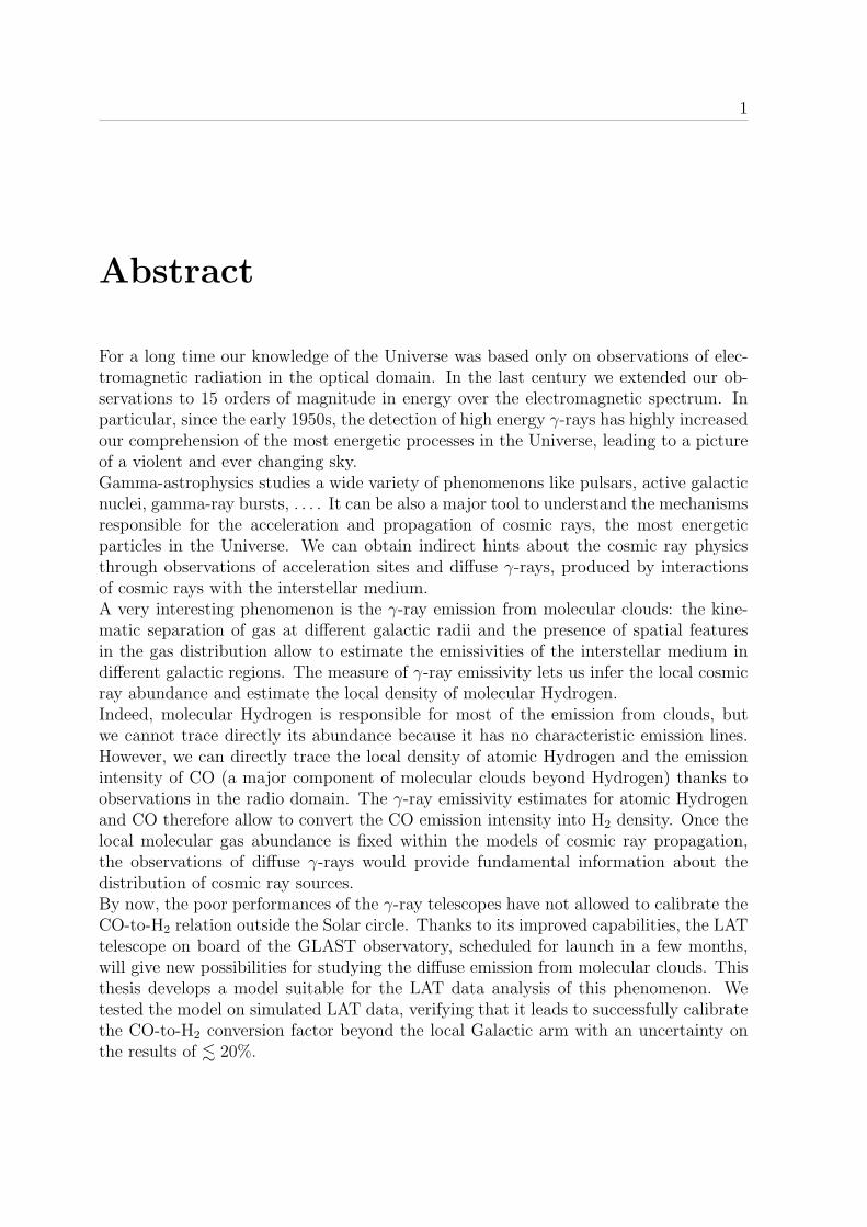
Abstract
For a long time our knowledge of the Universe was based only on observations of elec-tromagnetic radiation in the optical domain. In the last century we extended our ob-servations to 15 orders of magnitude in energy over the electromagnetic spectrum. Inparticular, since the early 1950s, the detection of high energy γ-rays has highly increasedour comprehension of the most energetic processes in the Universe, leading to a pictureof a violent and ever changing sky.Gamma-astrophysics studies a wide variety of phenomenons like pulsars, active galacticnuclei, gamma-ray bursts, . . . . It can be also a major tool to understand the mechanismsresponsible for the acceleration and propagation of cosmic rays, the most energeticparticles in the Universe. We can obtain indirect hints about the cosmic ray physicsthrough observations of acceleration sites and diffuse γ-rays, produced by interactionsof cosmic rays with the interstellar medium.A very interesting phenomenon is the γ-ray emission from molecular clouds: the kine-matic separation of gas at different galactic radii and the presence of spatial featuresin the gas distribution allow to estimate the emissivities of the interstellar medium indifferent galactic regions. The measure of γ-ray emissivity lets us infer the local cosmicray abundance and estimate the local density of molecular Hydrogen.Indeed, molecular Hydrogen is responsible for most of the emission from clouds, butwe cannot trace directly its abundance because it has no characteristic emission lines.However, we can directly trace the local density of atomic Hydrogen and the emissionintensity of CO (a major component of molecular clouds beyond Hydrogen) thanks toobservations in the radio domain. The γ-ray emissivity estimates for atomic Hydrogenand CO therefore allow to convert the CO emission intensity into H2 density. Once thelocal molecular gas abundance is fixed within the models of cosmic ray propagation,the observations of diffuse γ-rays would provide fundamental information about thedistribution of cosmic ray sources.By now, the poor performances of the γ-ray telescopes have not allowed to calibrate theCO-to-H2 relation outside the Solar circle. Thanks to its improved capabilities, the LATtelescope on board of the GLAST observatory, scheduled for launch in a few months,will give new possibilities for studying the diffuse emission from molecular clouds. Thisthesis develops a model suitable for the LAT data analysis of this phenomenon. Wetested the model on simulated LAT data, verifying that it leads to successfully calibratethe CO-to-H2 conversion factor beyond the local Galactic arm with an uncertainty onthe results of . 20%.
2
Prefazione
Per molto tempo la nostra conoscenza dell’Universo si e basata solo sull’osservazionedella radiazione visibile. Nell’ultimo secolo l’osservazione e stata estesa a 15 ordini digrandezza in energia sullo spettro elettromagnetico. In particolare, dall’inizio degli anni’50, la rivelazione di raggi γ di origine astrofisica ha accresciuto enormemente la nostracomprensione dei fenomeni di piu alta energia del cosmo, facendoci conoscere un cieloviolento e rapidamente variabile.Molti sono gli oggetti di studio dell’astrofisica γ: pulsar, nuclei galattici attivi, lampidi raggi gamma, . . . . L’astrofisica γ e una disciplina fondamentale anche per capire imeccanismi di accelerazione e propagazione dei raggi cosmici, le particelle di energiapiu alta nell’Universo. Informazioni indirette sulla fisica dei raggi cosmici si possonoottenere sia da osservazioni dei siti di accelerazione sia dei raggi γ diffusi, prodotti dalleinterazioni dei cosmici col mezzo interstellare.Un fenomeno molto interessante e l’emissione di raggi γ dalle nubi molecolari: la se-parazione cinematica del gas a diverse distanze dal centro della Galassia e la presenzadi addensamenti di gas con una ben caratterizzata distribuzione spaziale portano a sti-mare le emissivita del mezzo interstellare in differenti zone della Galassia. L’emissivitaγ permette di dedurre l’abbondanza locale di raggi cosmici e la densita di Idrogenomolecolare.L’Idrogeno molecolare infatti e responsabile della maggior parte dell’emissione di raggi γdalle nubi, ma non ne possiamo tracciare direttamente l’abbondanza perche non ha righedi emissione caratteristiche. Tuttavia possiamo misurare la densita locale di Idrogenoatomico e l’intensita di emissione del CO (una delle molecole piu abbondanti nelle nubioltre l’Idrogeno) grazie a osservazioni nella banda radio. La stima dell’emissivita γ perIdrogeno atomico e CO permette quindi di convertire l’intensita di emissione di COin densita di H2. Una volta fissata l’abbondanza locale di gas molecolare nei modellidi propagazione dei raggi cosmici, lo studio dei raggi γ diffusi permetterebbe di avereinformazioni fondamentali sulla distribuzione delle sorgenti dei raggi cosmici.Finora le caratteristiche dei telescopi per raggi γ non hanno permesso la calibrazionesperimentale della relazione tra CO e H2 in zone lontane dal sistema solare. Grazie allesue migliori prestazioni il telescopio LAT a bordo dell’osservatorio GLAST, in procintodi essere messo in orbita nei prossimi mesi, fornira nuove opportunita per lo studiodell’emissione di raggi γ dalle nubi molecolari. Questa tesi sviluppa un modello adeguatoper l’analisi dei dati di LAT relativamente a tale fenomeno. Il modello, testato su datidi LAT simulati, ha dimostrato di portare con successo alla calibrazione del rapportotra CO e H2 oltre il braccio locale della Galassia con incertezze sui risultati . 20%.
3
Chapter 1
The sky in gamma rays
In this chapter we summarize our current knowledge of the γ-ray sky. In section 1 wedescribe the physical processes involved in cosmic γ-ray production, propagation and de-tection. In section 2 we present the different kinds of γ-ray telescopes, with an historicaloverview of the most important instruments. Then we introduce the GLAST mission,which will improve our comprehension of the high energy sky in next years. In section3 we look at the known and candidate γ-ray sources, illustrating the most intriguingchallenges for γ-astrophysics.
1.1 Gamma ray production and detection
1.1.1 Production processes
Historically the name “γ-rays” was attributed to high energy electromagnetic radiationproduced in decay of excited nuclei. Now in astrophysics we call γ-rays the electromag-netic radiation at energies above 0.5 MeV. In the astrophysical context many processescan produce γ-rays, both thermal and nonthermal.Thermal radiation is produced by a large population of electromagnetically interactingparticles and fields in equilibrium. The spectrum, characterized by the temperature T ,follows the blackbody distribution, so the intensity I at the frequency ν is
I(ν) =8πhν3
c21
e−hν/kBT − 1
The radiation spectrum has a peak at a wavelength λmax
ε ' λmaxT
with the constant ε = 2.898 · 10−3 m K. So the radiation peak is in the optical regionfor T ∼ 6000 K (about the Sun’s surface temperature), while for γ-rays of 1 MeV T is2 · 109 K. The most typical γ-ray sources are in fact powered by nonthermal processes.
Synchrotron radiation
Let us consider a charged particle of mass m and charge q moving in a magnetic fieldB, with a pitch angle θ between the particle speed and the magnetic field direction. We
4 The sky in gamma rays
define the gyration frequency
νg =qB
2πmsin θ
The accelerated particle will emit photons with a peak at the frequency
νs =3
2γ2νg
if γ is the particle Lorentz factor. An electron with an energy of 1 GeV in the interstellarmagnetic field (∼ 1 µG) radiates synchrotron photons in the radio band. Synchrotronradiation may occur in the UV or X-ray region, and can reach γ-ray energies in extremecases such as on the surface of neutron stars (B ∼ 1010 G).
Bremsstrahlung
When a charged particle is decelerated by an electric field it emits photons. This phe-nomenon is called bremsstrahlung. For example, an electron interacting with a nucleuschanges its trajectory and produces radiation. We can distinguish thermal and nonther-mal bremsstrahlung, that is emission from charged particles in thermal equilibrium oremission from accelerated particles through a nonthermal process.Bremsstrahlung from energetic ions colliding with ambient electrons or nuclei is alwaysnegligible, so the most important process for γ-ray production is the interaction ofenergetic electrons with nuclei at low energies, and with both nuclei and electrons athigher energies.
ICS
We call ICS, Inverse Compton Scattering, the interaction of a low energy photon witha high energy particle, such as an electron, resulting in the production of a γ-ray, witha typical energy
Eγ ' 1.3
(Ee
TeV
)2 (Eph
2 · 10−4 eV
)GeV
ICS plays an important role in regions of high photon density.Relativistic electrons can also produce low energy photons by synchrotron radiationand then interact via ICS with them in the so called Synchrotron Self Compton (SSC)mechanism. The synchrotron photon frequency is νs ∝ B · E2
e , while the γ-photon willbe νIC ≈ νs · E2
e ∝ B · E4e .
Nuclear transitions
Nuclear levels have typical energy spacings of ∼ 1 MeV in magnitude. Radioactive decayof a freshly produced nucleus or energetic interactions can produce an excited state X∗,which generates a γ-ray through the decay
X∗ → X + γ
The most important lines for γ-ray astronomy are at 4.438 MeV (12C), 6.129 MeV (16O)and 1.809 MeV (26Mg). The cross section for excitation into these levels is maximizedin resonances, so nuclear lines trace low energy cosmic rays (CRs) and tell us aboutnucleosynthesis in different regions.
1.1 Gamma ray production and detection 5
Decays and annihilation
The most important decay for γ-ray production is neutral pion decay. Pions are gener-ated by strong interaction during collision of high energy cosmic rays with ambient gasor nuclei. The neutral pion π0 decays rapidly into two γ-rays, with an energy distribu-tion peaked at about 70 MeV in the pion rest frame. The π0 decay bump is offsettedand broadened by the momentum distribution of the high energy collisions producingpions.
Particle-antiparticle annihilation also produces γ-rays. The lightest pair is the electron-positron one, which gives two or more photons with a total energy of 1.022 MeV in theircenter of mass frame. In the same way hadronic and maybe exotic particle-antiparticlepairs can annihilate and generate γ-rays.
1.1.2 Gamma ray propagation
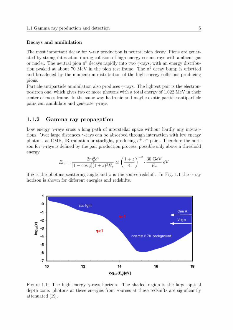
Low energy γ-rays cross a long path of interstellar space without hardly any interac-tions. Over large distances γ-rays can be absorbed through interaction with low energyphotons, as CMB, IR radiation or starlight, producing e+ e− pairs. Therefore the hori-zon for γ-rays is defined by the pair production process, possible only above a thresholdenergy
Eth =2m2
ec4
[1− cosφ](1 + z)2Eγ
'(
1 + z
4
)−2
· 30 GeV
Eγ
eV
if φ is the photons scattering angle and z is the source redshift. In Fig. 1.1 the γ-rayhorizon is shown for different energies and redshifts.
Figure 1.1: The high energy γ-rays horizon. The shaded region is the large opticaldepth zone: photons at these energies from sources at these redshifts are significantlyattenuated [19].
6 The sky in gamma rays
In addition, the attenuation of very high energy γ-rays is possible in regions of highdensity galactic interstellar radiation field, ISRF, as the galactic center.
1.1.3 Detection techniques
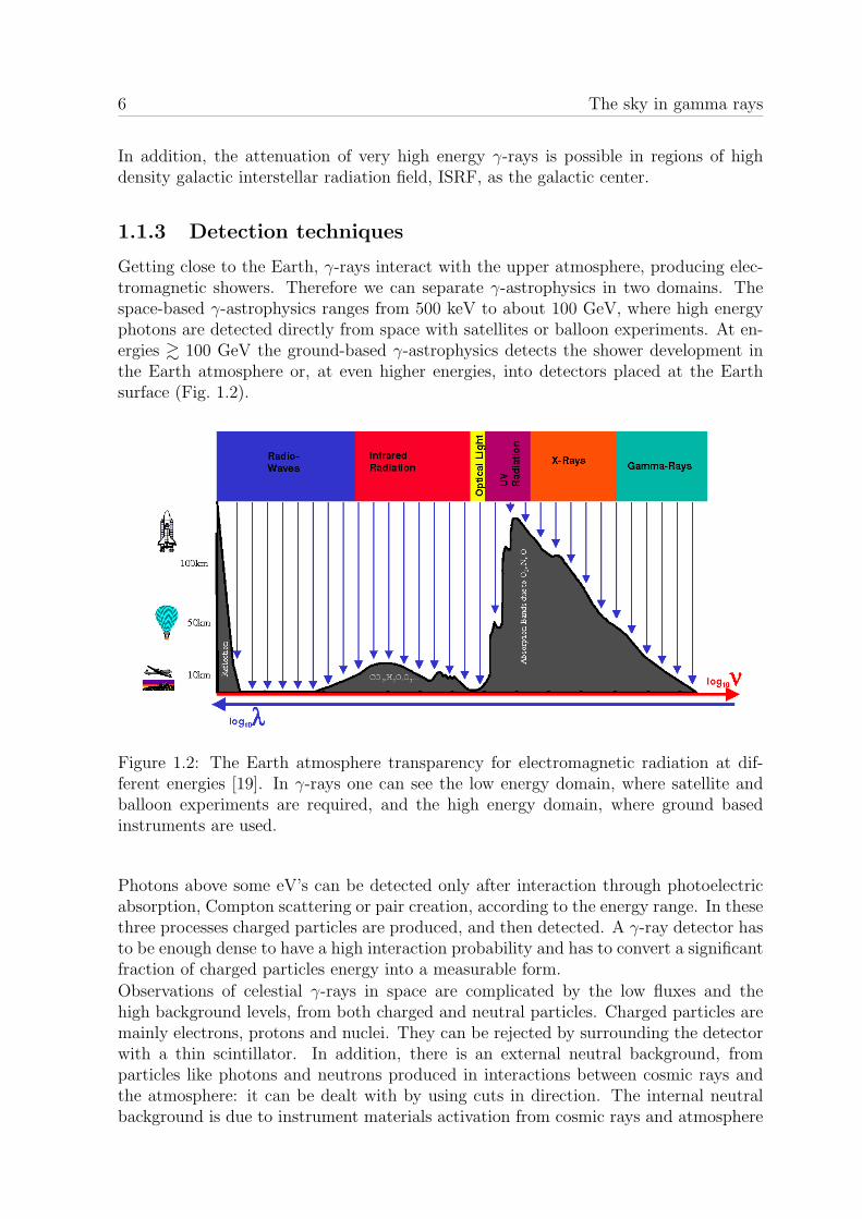
Getting close to the Earth, γ-rays interact with the upper atmosphere, producing elec-tromagnetic showers. Therefore we can separate γ-astrophysics in two domains. Thespace-based γ-astrophysics ranges from 500 keV to about 100 GeV, where high energyphotons are detected directly from space with satellites or balloon experiments. At en-ergies & 100 GeV the ground-based γ-astrophysics detects the shower development inthe Earth atmosphere or, at even higher energies, into detectors placed at the Earthsurface (Fig. 1.2).
Figure 1.2: The Earth atmosphere transparency for electromagnetic radiation at dif-ferent energies [19]. In γ-rays one can see the low energy domain, where satellite andballoon experiments are required, and the high energy domain, where ground basedinstruments are used.
Photons above some eV’s can be detected only after interaction through photoelectricabsorption, Compton scattering or pair creation, according to the energy range. In thesethree processes charged particles are produced, and then detected. A γ-ray detector hasto be enough dense to have a high interaction probability and has to convert a significantfraction of charged particles energy into a measurable form.
Observations of celestial γ-rays in space are complicated by the low fluxes and thehigh background levels, from both charged and neutral particles. Charged particles aremainly electrons, protons and nuclei. They can be rejected by surrounding the detectorwith a thin scintillator. In addition, there is an external neutral background, fromparticles like photons and neutrons produced in interactions between cosmic rays andthe atmosphere: it can be dealt with by using cuts in direction. The internal neutralbackground is due to instrument materials activation from cosmic rays and atmosphere
1.2 Gamma ray telescopes 7
neutrons and decay of natural radioactive elements. It can be minimized by lighteningthe detector structure.As told above, γ-rays entering the Earth atmosphere produce electromagnetic showers.Their detection is mainly carried out using the Cherenkov light produced by electronsand positrons in the shower: a charged particle moving through a transparent mediumfaster than the speed of light in that medium emits photons. There is a threshold energy
Eth = mc2 ·(
n√n2 − 1
)if n is the medium refraction index. Photons are emitted in a very short time (∼ ps) ina cone along the particle direction with an aperture angle θ
cos θ =1
βn
1.2 Gamma ray telescopes
A gamma ray telescope has not just to detect photons but also to measure their direction,energy and arrival time. Initial attempts to place upper limits on the fraction of γ-raysin the primary cosmic radiation were performed with balloon and rocket experimentsin the 1940s and early 1950s. Measurements with early instruments were often limitedby statistics or systematic uncertainties. Impressive progresses were made with newimaging techniques, depending on the energy range:
• collimators and modulation below some MeVs;
• Compton scattering-based techniques between 1-30 MeV;
• pair-tracking between 30 MeV and some hundreds GeV;
• air shower detection above some hundreds GeV.
Dedicated instruments have been developed for Gamma Ray Burst (GRB) detection.A general review about the γ-ray telescopes can be found in [33]: in this section we willintroduce the most important instruments.
1.2.1 Imaging via collimators
For X-rays, imaging is usually achieved by using collimators which define the instrumentfield of view. These collimators are arrays of tubes with absorbing walls, so only X-rayswith a path parallel to the tube can reach the detector. Because of the high penetrationpower of γ-rays, these collimators can not be used at γ-ray energies: too much materialwould be needed and too much background radiation would be produced.Actively collimated γ-ray telescopes, i.e. telescopes collimated with an active shield,like a plastic scintillator, have been successfully used: OSO-3, the γ-ray experiment onboard of the Solar-Maximum Mission (SMM), the Gamma Ray Imaging Spectrometer(GRIS) and the Oriented Scintillation-Spectrometer Experiment (OSSE).

8 The sky in gamma rays
OSSE
The Oriented Scintillation-Spectrometer Experiment, OSSE, was one of the four instru-ments on the Compton Gamma Ray Observatory, CGRO, the NASA large observatorythat operated from 1991 to 2000 (Fig. 1.3), giving the first complete γ-ray sky survey.
Figure 1.3: Schematic view of the CGRO observatory.
OSSE consisted of four identical detectors, that could be independently rotated within192. The main element of each detector was a phosphor-sandwich consisting of aNaI(Tl) crystal with a diameter of 33 cm and a 7.6 cm thick CsI(Na) crystal at therear side. A passive Tungsten collimator was placed on the front side, defining a fieldof view of 3.8×11.4. This detector was surrounded by an annular shield of NaI(Tl)crystals. The different scintillation decay-time constants of NaI and CsI were used todistinguish γ-rays from above and below. The spectral resolution was controlled via thePMTs voltage, using a calibration source of 60Co. OSSE had an effective area of 400cm2 around 1 MeV, with an energy resolution of about 5-10%.
1.2.2 Imaging via modulation techniques
A γ-ray telescope with a wide field of view can reach a good angular resolution modulat-ing the signal from the source to the detector. The first modulation technique developedwas occultation. From the occulter and detector position and given the time when thesource vanishes, one can gain information about the source position. High positionalresolution is reached when the distance between detector and occulter is large: thistechnique is especially used to study the Moon using the Earth occultation.The best modulation technique uses arrays of opaque and transparent elements arrangedin a regular pattern, called coded masks. A point source produces a shadow of thecoded mask onto the detector, the shadowgram. From the shadowgram one can obtainthe source position using deconvolution algorithms. The occulted part of the detector
1.2 Gamma ray telescopes 9
allows an independent determination of the background. The most important codedmask telescopes have been SIGMA and INTEGRAL.
SIGMA
In 1989 the Russian mission GRANAT began, transporting on board the French tele-scope SIGMA, which gave the first survey in the transitional region between hard X-raysand soft γ-rays (35 keV - 1 MeV). It mainly observed the galactic center, detecting about30 sources and discovering the so called galactic microquasars, objects that show a jetstructure emanating from a compact radio cone. The mask was made of Tungstenelements and a shield of CsI scintillator was used as an aperture-defining device.
INTEGRAL
The INTErnational Gamma Ray Astrophysics Laboratory (INTEGRAL), launched in2002 by ESA, transports two instruments based on SIGMA design, IBIS and SPI, bothoperating from 15 keV to 10 MeV. There are two additional instruments, JEM-X, an X-ray monitor which works from 3 keV to 35 keV, and OMC, an optical telescope observingbetween 500 and 850 nm.The Imager on Board of the INTEGRAL Satellite, IBIS, has an array of 53×53 opaqueelements which allows an angular resolution of 12 arcsec. It consists of two planes: theupper layer, made up of 16348 CdTe pixels (for a total area of 2621 cm2), is used tomeasure between 15 keV and 400 keV with an energy resolution of 7%; the lower layer,made of 4096 CsI scintillators (total area 3318 cm2), for the detection of γ-rays from200 keV to 10 MeV with a typical energy resolution of 6%. The aperture is defined byan active BGO shield around the detector and a passive Tungsten collimator betweenthe mask and the BGO shield.The SPectrometer on Integral, SPI, has a coded mask like IBIS, but its main detectorconsists of an array of 19 Ge crystals. This detector allows an energy resolution of 0.2%between 20 keV and 8 MeV. The whole detector is surrounded by a BGO active shield.
1.2.3 Compton telescopes
The absorption probability for γ-rays in matter reaches a minimum in the range from1 to 5 MeV, so the imaging techniques described above do not work well at theseenergies. Here the dominant interaction mechanism is Compton scattering: a photoninteracts with an electron, producing a photon with a final energy Ef , depending on thescattering angle ϕ according to the formula
Ef =mec
2Eγ
Eγ(1− cosϕ) +mec2
Compton telescopes are used up to ∼ 20 MeV, although pair production becomes dom-inant over 5 MeV, due to the better performances in term of identification of photons,angular and energy resolution.A Compton telescope consists of two detector planes, the scatter and the absorptionplane, separated by a ∼ 2 m distance. According to the Klein-Nishina cross section (in

10 The sky in gamma rays
the limit Eγ/mec2 1)
σKN = r20 ·πmec
2
Eγ
·[ln
(2Eγ
mec2+
1
2
)](with the classical electron radius r0 = e2/4πε0mec
2 = 2.8 · 10−15 m) the Comptoninteraction probability is proportional to the electron density, i.e. to the atomic numberZ, while the photoelectric effect and pair production probability is proportional to Zn
with n ≥ 2. In the scatter detector Compton process has to be favored, so a low-Z material must be used. The absorption detector has to absorb the energy of thescattered photon, therefore it must be built using a high-Z material.
In an ideal case the measurement of the energy losses in the scatter detector E1 and inthe absorption detector E2 would allow the evaluation of the incoming photon energyand scattering angle.
Eγ = E1 + E2
ϕ = arccos
[1−mec
2 ·(
1
E2
− 1
E1 + E2
)]To estimate photon directions one needs to know the interaction positions, either usingdetector planes made of small modules or applying the Anger-camera technique (thepulse heights of PMTs viewing a scintillator allow to know the interaction position).An obvious disadvantage of Compton telescopes is that the infalling direction of γ-raysis not uniquely identified: the only thing one can reconstruct is the event circle, whoseopening is given by the scattering angle ϕ (Fig. 1.4).
E2
E1
event circle
ϕscatter detector
absorption detector
Figure 1.4: Schematic view of a Compton telescope working principle.
After the first Compton telescopes on balloon experiments with poor performances, abreakthrough was achieved with COMPTEL.
1.2 Gamma ray telescopes 11
COMPTEL
COMPTEL was the first Compton telescope flying on a satellite, the CGRO. It detectedphotons from 700 keV to 30 MeV, its main components were:
• a scatter detector array of liquid organic scintillator;
• an absorption detector array of NaI(Tl) crystals;
• anticoincidence shields made up of plastic scintillator;
• tagged 60Co sources for instrument calibration.
The Anger-camera technique allowed to measure photon direction within an event circleof ∼ 0.76 radius.The COMPTEL effective area ranged from 10 cm2 to 50 cm2, the energy resolution from3% to 15%. The point source sensitivity for a two week observation was 10−5 cm−2 s−1.
1.2.4 Pair-tracking telescopes
For γ-rays with energy & 20 MeV, pair-tracking telescopes are used, because the mostimportant interaction process is pair production. A pair-tracking telescope usually hasthe following parts:
• an anticoincidence shield;
• a conversion device (because the conversion probability is proportional to Z2, ithas to consist of a high Z material like Tungsten or Tantalum);
• a pair-tracking device (in past missions a spark chamber);
• a time of flight measurement system or a Cherenkov detector, to help the antico-incidence shield in rejecting the background;
• a calorimeter for the absorption and measurement of electromagnetic energy.
The first pair-tracking telescope featuring a good signal to noise ratio was SAS-2,launched in 1972. Unfortunately this experiment malfunctioned after half a year. Themost important are up to now COS-B, launched in 1975, EGRET, on board of theCGRO, and the recently launched Italian telescope AGILE.
COS-B
COS-B realized the first Milky-Way map, detecting 24 galactic sources and also anextragalactic source (the active galaxy 3C 273). The COS-B core was a gas filled wire-grid spark chamber with 16 planes. Below its 12 top grids Tungsten sheets were mountedas converter foils. The calorimeter was composed of CsI(Tl) crystals, for a thickness of4.7 radiation lengths. COS-B was sensitive to γ-rays from 30 MeV to several GeVs overa field of view of about 2 sr. It had an energy resolution of 10% FWHM at 100 MeVand an angular resolution of 2.5 at 2 GeV.

12 The sky in gamma rays
EGRET
The Energetic Gamma Ray Experiment Telescope, EGRET, was the CGRO experimentsensitive to γ-rays in the energy range from 20 MeV to 30 GeV (Fig. 1.5). Its central
Figure 1.5: The EGRET telescope [24].
unit was a multilevel wire-grid spark chamber with Tantalum conversion layers. It hada trigger telescope consisting of plastic scintillator sheets into the lower part of the sparkchamber. A time of flight measurement discriminated between upward and downwardmoving charged particles. The calorimeter was made of NaI(Tl) crystals. The fieldof view was about 0.5 sr, with an energy resolution of 0.5 at 10 GeV. EGRET hadan energy resolution of 20-25% FWHM, an effective area of 1000 cm2 on axis. Thesensitivity limit at 3σ corresponded to a minimum flux of 10−7 cm−2 s−1.
AGILE
AGILE (Astro-rivelatore Gamma a Immagini LEggero) was launched in April 2007. Itsmain instrument is the Gamma-Ray Imaging Detector (GRID), operating between 30MeV and 50 GeV, which consists of a plastic scintillator anticoincidence system, a Si-Wtracker and a CsI calorimeter. In contrast with previous generation instruments it doesnot require gas operations and high voltages. The new tracking technique allows a goodangular resolution (15′ for intense sources), an unprecedentedly large field of view ofabout 2.5 sr and an efficiency comparable to that of EGRET.
1.2.5 Cherenkov telescopes
Below ∼100 GeV the atmosphere opaqueness requires the instruments described aboveto be carried by balloons or satellites. Above ∼100 GeV γ-rays are so highly penetratingthat they will be absorbed only at lower heights producing large particle showers.

1.2 Gamma ray telescopes 13
At energies of some hundreds GeV the atmosphere itself can be used as sensitive medium:the Cherenkov light produced by the shower in the atmosphere is detected, using Hillastechnique (1985) to discriminate γ-rays from proton showers. The Imaging AtmosphericCherenkov Technique (IACT), which allows to reach the 99.7% of hadronic backgroundrejection, was first used for the Whipple telescope, which detected in 1989 the first TeVγ-ray from the Crab Nebula. After the HEGRA (High Energy Gamma Ray Astronomy)telescope in late 1990s, the most important IACT instruments are now MAGIC andVERITAS in the North emisphere and HESS and CANGAROO in the South emisphere.At TeV energies the air shower can be better detected with a ground based detector. Itcan be a water Cherenkov detector, which allows a very large field of view and continuousoperation, as in the Milagro telescope.
MAGIC
The MAGIC (Major Atmospheric Gamma Imaging Cherenkov) telescope is located onthe Canary Island of La Palma, at 2200 m above the sea level. It is possible to positionthe telescope in about 20 s to target any point of the observable sky. MAGIC is charac-terized by the widest light collection surface (240 m2) in IACTs: the mirror is composedof nearly 1000 elements forming a parabolic dish of 17 m diameter. The high resolutioncamera of 4 diameter is composed of 576 hemispherical PMTs. The Cherenkov photonsreflected in the mirrors are seen by the camera as an image whose characteristics allowto identify the recorded particles as a γ-ray shower, specify its direction and energy.MAGIC detects γ-rays with energy & 50 GeV, has an energy resolution of about 20 %at 1 TeV and an accuracy in source location of 0.1.
Milagro
Milagro, located near Los Alamos, consists in a 80 m × 60 m × 8 m pond of waterwith a light tight cover. It contains 723 PMTs, placed on a 3 m × 3 m grid. Usingthe relative timing of the PMTs the direction of the infalling particle or γ-ray can bereconstructed with an accuracy of about 1. Milagro is sensitive to γ-rays with energies> 100 GeV.
1.2.6 GRB instruments
GRB instruments need to have a large field of view, since the duration of bursts is ofthe order of seconds and their occurrence rate is about one per day over the whole sky.At this time, the most successful instrument is BATSE, on board of the CGRO.
BATSE
The Burst and Transient Source Experiment was a full sky monitor consisting of eightthin scintillator modules, one on each corner of CGRO. Each detector plane was orientedin a different direction. From the relative intensities the direction of a γ-ray burstcould be deduced with an accuracy of 1 to 10. Each of the modules had a large areadetector, optimized for sensitivity and directional response, and a spectroscopy detector,optimized for energy coverage and energy resolution. Both detectors were made of NaIcrystals. A plastic scintillator acted as active shield for the charged particle background.
14 The sky in gamma rays
1.2.7 The GLAST mission
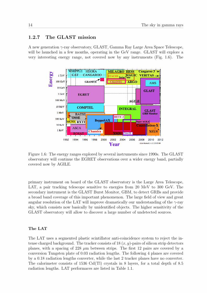
A new generation γ-ray observatory, GLAST, Gamma Ray Large Area Space Telescope,will be launched in a few months, operating in the GeV range. GLAST will explore avery interesting energy range, not covered now by any instruments (Fig. 1.6). The
Figure 1.6: The energy ranges explored by several instruments since 1990s. The GLASTobservatory will continue the EGRET observations over a wider energy band, partiallycovered now by AGILE.
primary instrument on board of the GLAST observatory is the Large Area Telescope,LAT, a pair tracking telescope sensitive to energies from 20 MeV to 300 GeV. Thesecondary instrument is the GLAST Burst Monitor, GBM, to detect GRBs and providea broad band coverage of this important phenomenon. The large field of view and greatangular resolution of the LAT will improve dramatically our understanding of the γ-raysky, which consists now basically by unidentified objects. The higher sensitivity of theGLAST observatory will allow to discover a large number of undetected sources.
The LAT
The LAT uses a segmented plastic scintillator anti-coincidence system to reject the in-tense charged background. The tracker consists of 18 (x, y)-pairs of silicon strip detectorsplanes, with a spacing of 228 µm between strips. The first 12 pairs are covered by aconversion Tungsten plate of 0.03 radiation lengths. The following 4 planes are coveredby a 0.18 radiation lengths converter, while the last 2 tracker planes have no converter.The calorimeter consists of 1536 CsI(Tl) crystals in 8 layers, for a total depth of 8.5radiation lengths. LAT performaces are listed in Table 1.1.

1.3 Gamma ray sources 15
LAT EGRET
Energy range 20 MeV - 300 GeV 20 MeV - 30 GeVPeak effective area >8000 cm2 1500 cm2
Field of view >1.5 sr 0.5 srAngular resolution <3.5 (100 MeV) 5.8 (100 MeV)Energy resolution <10% 10%Deadtime per event <100 µs 100 msSource location determination <0.5′ 15′
Point source sensitivity < 6 · 10−9 cm−2 s−1 ∼ 10−7 cm−2 s−1
Table 1.1: LAT science requirements compared with EGRET performances [1].
The GBM
The GLAST Burst Monitor includes 12 Sodium Iodide (NaI) scintillation detectors and2 Bismuth Germanate (BGO) scintillation detectors. The NaI detectors cover the lowerpart of the energy range, from a few keV to about 1 MeV and provide burst triggers andlocations. The BGO detectors cover the energy range of 150 keV to 30 MeV, providing agood overlap with the NaI at the lower end, and with the LAT at the high end. Sciencerequirements for GBM are reported in Table 1.2.
GBM BATSE
Energy range < 10 keV - 25 MeV 25 keV - 10 MeVField of view all sky not occulted by the EarthEnergy resolution <10% < 10%Deadtime per event <15 µsBurst sensitivity < 0.5 cm−2 s−1 0.2 cm−2 s−1
Alert GRB location ∼15 ∼25
Final GRB location ∼3 1.7
Table 1.2: GBM science requirements compared with BATSE performances [1].
1.3 Gamma ray sources
1.3.1 Solar system objects
Due to their proximity, Solar system objects, like the Sun and the Moon, can be verybrilliant γ-ray sources. The Sun is an active γ-ray source, whereas γ-rays from the Moonare produced by cosmic ray interactions on its surface. There is obviously a strong γ-rayalbedo from the Earth atmosphere, but it is usually considered as a background.
16 The sky in gamma rays
The Sun as a gamma-ray source
The first detection of γ-rays from the Sun was made in the late 1950s. Since the 1940sit has been known that high energy particles are produced in solar flares, so the flaringSun was recognized as γ-ray source. The flaring Sun can easily outshine in the MeVdomain any other source. There are many reasons to assume that the quiet Sun couldbe a γ-ray source as well and several emission mechanisms have been proposed:
• decay of long lived radioactive nuclei produced in flares such as 54Mn or 56Co;
• interaction of high energy particles, accelerated by a shock wave and then movingback to the Sun along its magnetic field lines, with the solar atmosphere;
• the neutron capture line on H at 2.2 MeV (with a flux limit of 5.1 · 10−5 cm−2 s−1
from the SMM);
• the positron annihilation line at 0.511 MeV.
The two lines would have a very narrow width because the processes take place whenparticles are at rest.A solar flare is defined as a process that occurs when a quick (a few seconds) release ofmagnetic energy takes place in a relatively small volume of the Sun atmosphere. Thesolar flare emission is originated from accelerated particles. According to the parentparticle, the radiation can be classified as electron-induced or nucleon-induced emission.During the flare, accelerated particles generate γ-rays via bremsstrahlung or throughthe production of secondaries (positrons, neutrons, radioactive nuclei, . . . ).Spectral analysis of the flares shows that high energy protons and electrons are usuallyproduced in about the same proportion, but there are also electron-dominated events.The primary proton spectrum shows a cut-off at energies above 200 MeV per nucleon.
Gamma-ray albedo from the Moon
The Moon has been detected by EGRET as a point source with a steep spectrum above1 GeV. Whereas the Sun and the Earth albedo γ-rays come from interactions with theirgaseous atmosphere, the Moon emits albedo γ-rays due to CR interactions with its solidsurface. This makes its albedo spectrum unique [43]. The secondary particle cascadefrom CRs hitting the Moon surface at small zenith angles develops deep into the rock,making it difficult for γ-rays to get out. A small fraction of all produced pions, thesplash albedo pions, are the lowest energy ones, so they produce the soft spectrum.High energy γ-rays can be produced by CRs hitting the Moon surface in a close-totangential direction but, since the Moon is a solid target, only photons emitted in asmall solid angle can be observed.
1.3.2 Pulsars
In 1967 a pulsing radio signal was explained as emission from a rotating, magnetizedneutron star called pulsar, PSR, (Pacini and Gold, 1968). Now we know about 1500radio pulsars: the range of periods P extends from a few milliseconds to some seconds,while the period first derivative P ranges from 10−21 to 10−11 s/s.
1.3 Gamma ray sources 17
For stars with a core mass from about 1.44 to 3.6 M, after the nuclear fuel is exhaustedthe outer layers are ejected and the central core contracts and cools to form a compactobject of radius ∼10 km with density of the order of 1015 g cm−3. Matter, present aselectrons and nuclei, recombines via inverse β-decay to form neutrons. The pressure ofthe degenerate Fermi gas of neutrons is sufficient in the above mass range to stabilizethe stellar core. Conservation of angular momentum increases the rotational frequencyof about 1010 times. Because for a relativistically streaming plasma under very generalmagnetohydrodynamics assumptions the magnetic flux through any surface is conserved[12], the magnetic field increases from values typical in a normal star (100 G) to valuesof the order of 1010-1012 G. The star is transformed into a spinning magnetic dipole,which radiates electromagnetic energy.Electric field has a discontinuity at the stellar surface that implies a surface charge layer.Charges are therefore ejected from the surface and fill the pulsar magnetosphere, wherethey arrange themselves until the electric and magnetic forces are in equilibrium. Therequired charge density, found by Goldreich and Julian, is
nGJ =~ω · ~B2πc
= 7 · 1010 B‖(1012 G)P−1 cm−3
where B‖ is the field component parallel to ~ω. Static equilibrium in the pulsar magne-tosphere is forbidden by special relativity: at a distance rc = c/ω (the light cylinder)particles and fields would have to corotate at the speed of light. Field lines trying toextend across rc are forced open to the outside and release their charges into the pulsarwind zone. In the inner magnetosphere this outflow leads to a charge deficit in thegap region above the magnetic pole, the polar cap, and between the zero charge densitysurface (nGJ = 0) and the magnetosphere close to the light cylinder, the outer gap. Inthese gap regions the electrostatic potential of the rotating dipole is not balanced bycharges and is available to accelerate particles to very high energies.The CGRO identified seven γ-ray pulsars with very high confidence, including the threemost brilliant point-like sources of the GeV sky: Vela, Crab and Geminga. Their lightcurves (photon histogram versus pulse phase) show common features like a double peakand energy dependence. The maximum power per frequency interval is found in theγ-ray band, but no pulsed emission has been detected above 30 GeV, so a high energycut-off mechanism is likely. GLAST is expected to detect a large number of pulsars andto give a strong contribution in the comprehension of emission mechanisms.
1.3.3 Supernova remnants
Supernova Remnants (SNRs) are the objects produced by the explosion of a massivestar at the end of its life. This explosion, observed as a supernova, SN, is one of themost energetic events in the universe and produces primarily three effects:
• it blows a hole in the interstellar medium (ISM), that rapidly expands until itreaches up to several hundred light years in diameter; the temperature in thisbubble is very high (several millions K) so the ISM is strongly modified;
• the shock wave of this explosion is believed to be important in the acceleration ofcosmic rays and in the formation of new stars from the interstellar gas;
18 The sky in gamma rays
• it distributes various elements through the ISM, in particular it is the principalsource of elements heavier than He.
Observations allow to distinguish three types of SNRs:
Shell-type SNRs show a ring structure, the edge of the bubble heated and stirred upby the shock wave front; shell-type are more than 80% of known SNRs.
Plerions or Crab-like SNRs are roughly spherical objects with a filled center, which isthought to indicate the presence of a pulsar.
Composite SNRs share common features with plerions and shell-type SNRs, i.e. a shellof hot gas with a small central synchrotron nebula.
In 1953 Shklovsky suggested that optical emission from the Crab nebula might be syn-chrotron emission from relativistic electrons: the link between SNRs and particle ac-celeration was established. In the third EGRET catalog 11 unidentified sources can beassociated with known SNRs. High energy γ-ray emission from SNRs is expected as aresult of the interaction of energetic particles with the remnant itself and the surround-ing matter and fields. These expectations are supported by the IACT CANGAROO,which detected photons with energy greater than 1 TeV from SN 1006.
1.3.4 X-ray binaries
In 1967 optical spectroscopy of the supergiant HD 226868, the optical counterpart ofCygnus X-1, the first X-ray source detected in the Cygnus region, revealed a variation inradial velocity, indicating orbital motion in a binary system. The mass function derivedfrom the orbital period and amplitude in radial velocity implied a mass of the compactobject greater than 3 M, the maximum possible mass of a neutron star, and thereforestrongly suggested the presence of a black hole. X-Ray Binaries, XRBs, consist generallyof a binary-star system with one component being a compact object at the end of itsstellar evolution (a white dwarf, a neutron star or a black hole). Their X-ray luminosityis powered by accretion of matter from the companion star onto the compact object.At γ-ray energies of about 1 MeV only two sources have been detected by COMPTEL:the persistent source Cyg X-1 and the transient X-ray nova GRO J0422+32. In 1994 for12 days EGRET detected a source positionally coincident with Cen X-3. Ground-basedtelescopes have detected some XRBs, including Cyg X-1, now called γ-ray binaries.The high energy emission of the black hole system is generally found to be variable influx on all accessible time scales:
• the long term (months to year) light curves show three different types, with a fastrise (a few days) and a slower decay (several weeks), with multiple outbursts slowrising and decaying or with a persistent emission;
• there is also a strong and rapid aperiodic variability from time scales of hundredsof seconds down to ms.
Future accurate measurements of the XRB spectral shape between 500 keV and severalMeV will provide crucial information about the emission mechanisms and the relation-ship between thermal and nonthermal processes in the accretion disc. Instruments with
1.3 Gamma ray sources 19
improved sensitivity and a larger field of view, like GLAST, offer the possibility to detectother sources like Cen X-3 and clearly identify them with an XRB. Moreover the detec-tion of high energy γ-rays, also by Cherenkov telescopes, can provide strong evidence ofparticle acceleration in those fast rotating systems.
1.3.5 Active galactic nuclei
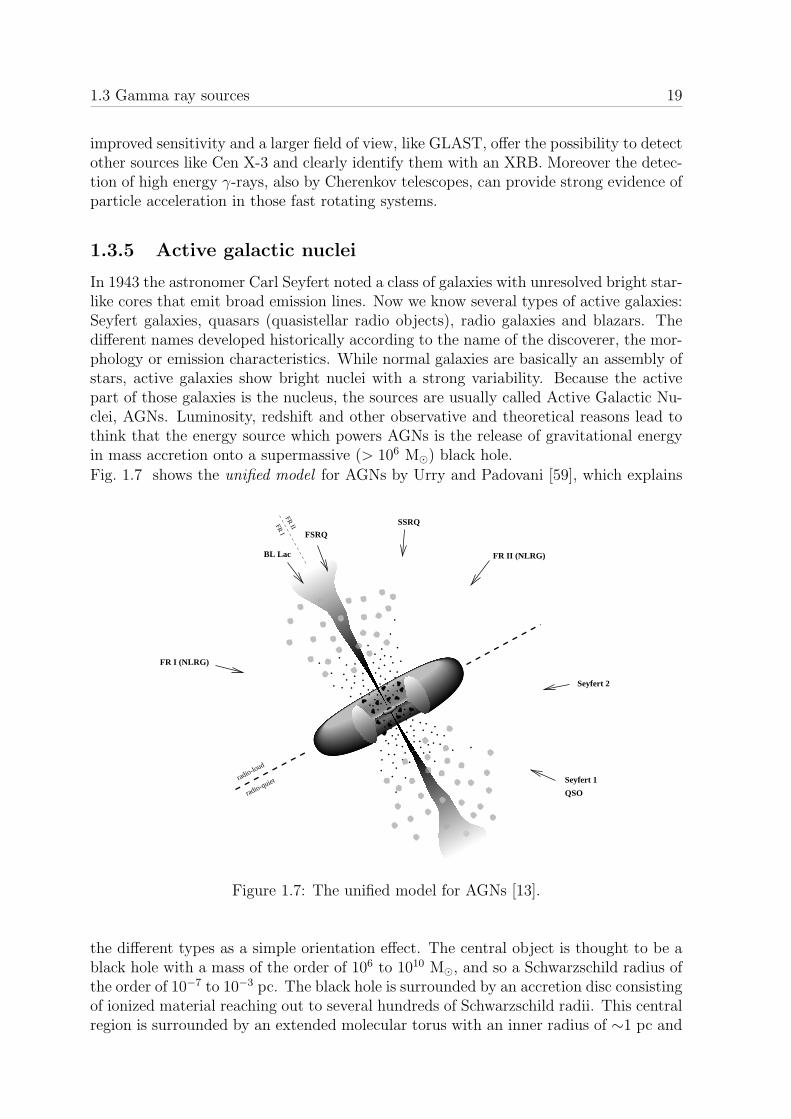
In 1943 the astronomer Carl Seyfert noted a class of galaxies with unresolved bright star-like cores that emit broad emission lines. Now we know several types of active galaxies:Seyfert galaxies, quasars (quasistellar radio objects), radio galaxies and blazars. Thedifferent names developed historically according to the name of the discoverer, the mor-phology or emission characteristics. While normal galaxies are basically an assembly ofstars, active galaxies show bright nuclei with a strong variability. Because the activepart of those galaxies is the nucleus, the sources are usually called Active Galactic Nu-clei, AGNs. Luminosity, redshift and other observative and theoretical reasons lead tothink that the energy source which powers AGNs is the release of gravitational energyin mass accretion onto a supermassive (> 106 M) black hole.Fig. 1.7 shows the unified model for AGNs by Urry and Padovani [59], which explains
FR II (NLRG)
SSRQ
FR I (NLRG)
Seyfert 1
QSO
FR IIFR
I
radio-quiet
BL Lac
FSRQ
Seyfert 2
radio-loud
Figure 1.7: The unified model for AGNs [13].
the different types as a simple orientation effect. The central object is thought to be ablack hole with a mass of the order of 106 to 1010 M, and so a Schwarzschild radius ofthe order of 10−7 to 10−3 pc. The black hole is surrounded by an accretion disc consistingof ionized material reaching out to several hundreds of Schwarzschild radii. This centralregion is surrounded by an extended molecular torus with an inner radius of ∼1 pc and

20 The sky in gamma rays
an outer radius of ∼15 pc. Fast moving gas clouds exist within the molecular torus and,ionized by the accretion disc radiation, emit the observed broad lines. Further out cloudsmove slower and produce the narrow lines. A strong jet of relativistic particles emanatesperpendicular to the plane of the accretion disc. If we look along the jet axis (. 10)we observe a blazar or a quasar or a Seyfert type 1 galaxy with a flat radio spectrum.A steep spectrum quasar or a Seyfert type 2 galaxy is observed at offset angles of theorder of 30. A typical radio galaxy, showing two oppositely aligned jets, is observed atviewing angles perpendicular to the jet axis. This scenario leaves unresolved questionsabout the efficiency and the relative contribution of the different emission mechanisms.In addition, it neglects evolution and variability, which are probably very important forthese galaxies.
Blazars have been detected in γ-rays by EGRET and by Whipple and other IACTsat very high energies. The most intriguing results are the short time variability andthe inferred huge γ-ray luminosity. These facts are explained assuming that we areviewing almost along the axis of a relativistically outflowing plasma jet. Seyfert andradio galaxies have been detected by OSSE and BATSE at energies between 50 and 150keV. Only Centaurus A have been detected at MeV energies by COMPTEL and maybeabove 100 MeV by EGRET.
1.3.6 Gamma ray bursts
In 1967 the detection of inexplicable increases in the count rate of γ-ray detectors onboard of the Vela satellites opened the GRB puzzle. From arrival times a solar andterrestrial origin could be excluded. In 1976 the first dedicated burst instrument waslaunched: it proved that the burst location was inconsistent with all candidate sourceslike pulsars, SNRs . . . Subsequently more bursts were detected with different temporaland spectral behaviors. The CGRO, with EGRET and BATSE, measured location andspectra of more than 2000 bursts.
No characteristic energies are evident in GRB spectra. Measured spectra can be de-scribed by the Band function [7]
N(E) =
AEα e−E/E0 E ≤ Eb
A′Eβ E ≥ Eb
with Eb = (α − β)E0 and A′ such that N is continuous. Typical values for parametersare α = −1, β = −2 and E0 = 150 keV. The spatial distribution of bursts is isotropicbut inhomogeneous in redshift.
The discovery of optical counterparts with redshifted absorption lines pushed the originof γ-ray bursts to cosmological distances. Cosmological models naturally explain theobserved isotropy and inhomogeneity, because galaxy distribution is isotropic, but thetemporal evolution and relativistic effects can produce the observed deficiency of weakbursts. The γ-ray burst process can be separated into two steps: the initial productionof energy and the subsequent dissipation creating γ-rays. From causality considerations,the initial dimensions of the source are constrained by the shortest time variation of theburst (∼ 10−3 s), which leads to an upper limit of about 100 km.
1.3 Gamma ray sources 21
1.3.7 Dark matter
The existence of Dark Matter (DM), matter not electromagnetically interacting, wasproposed to explain the rotational curves of galaxies, and now is strongly supported byCMB power spectrum, large scale structures and many other astronomical observations.The first particle candidates for DM were neutrinos, but recent measurements gave anupper limit of ∼ 7 eV for the sum of the three neutrinos masses, and more, to matchthe large scale structure properties, DM must be cold DM, i.e. matter not relativisticat decoupling [8]. The DM candidates have therefore to be Weakly Interacting MassiveParticles, WIMPs. Now the best WIMP candidate is the Lightest Super Partner (LSP)of the Standard Model supersymmetric extensions. Supersymmetric particles have beenoriginally introduced to solve problems of the Subnuclear Physics Standard Model, likethe hierarchy problem.These supersymmetric theories (SUSY) lead to the existence of a massive relic particle,the LSP, in most scenarios the neutralino, a Majorana particle superposition of thesuperpartners of Z0, photon and Higgs boson. Two neutralinos can annihilate, producinghigh energy secondaries, among them γ-rays. If neutralinos made up the dark matter,they would have non relativistic velocities, so the neutralino annihilation into γ− γ andγ −Z0 could produce lines at energies Eγ = mχ and Eγ = mχ(1−m2
Z/4m2χ). However,
these lines are suppressed according to SUSY theories. There would be also a continuumγ-ray spectrum from annihilation in high energy pairs like b− b.
1.3.8 Diffuse gamma rays
Diffuse γ-rays dominate the γ-ray sky, constituting almost the 90% of the total lumi-nosity at high energies. The diffuse emission consists basically of three components:
• the galactic γ-ray diffuse emission, coming from interaction processes in the ISM;
• the EGRB, Extragalactic Gamma Ray Background;
• the contribution of unresolved sources.
The diffuse galactic emission is produced basically by interaction of high energy cosmicrays with the ISM, so it can provide fundamental information about both CR accelera-tion and propagation and the ISM itself. Because the Galaxy is almost transparent tohigh energy γ-rays, the galactic diffuse γ-ray emission is the line of sight integral overthe emissivity of the ISM. It has been shown that there is a generally decreasing γ-rayemissivity with galactocentric radius. The galactic γ-ray background may also containsignature of new physics, like DM signals (see 1.3.7). Continuum γ-emission leads to in-fer the global distribution of CRs, in particular, while electrons have to be galactic, sincethe energy losses via ICS on the CMB photons prevent propagation from one galaxy toanother, for protons and nuclei there has been a long debate. The CGRO observationshave revealed that the γ-ray flux from the Small Magellanic Cloud is strongly inconsis-tent with CR protons having uniform density in space. Therefore the bulk of the locallyobserved protons at GeV energies must be galactic. EGRET data showed an intriguingexcess in emission at about 1 GeV with respect to conventional models of CRs, leadingto new theoretical developments. The physics of the galactic diffuse γ-rays will be thesubject of chapter 2.
22 The sky in gamma rays
The EGRB is not well understood. It might contain information about early stages ofthe Universe and new physics: potentially the EGRB can provide very important in-formation about the phase of baryon-antibaryon annihilation, evaporation of primordialblack holes and annihilation of WIMPS. However, its spectrum is poorly determined,because its estimate depends strongly on the model adopted for the galactic emission.To study the EGRB a better knowledge about the galactic diffuse emission and CRpropagation is required. The near future prospects are encouraging, both for direct CRmeasurements, with PAMELA, BESS and AMS and for γ-ray astrophysics with theGLAST observatory.
23
Chapter 2
Diffuse galactic gamma rays:a cosmic ray tracer
In this chapter we discuss the physics of galactic diffuse gamma rays, produced by in-teractions of high energy cosmic rays with the interstellar medium. In section 1 wesummarize our knowledge about cosmic rays: the Sun modulation of charged particlesin the Earth proximity, direct observations of extrasolar cosmic rays and interactionprocesses in the interstellar medium leading to indirect observations. Then, in section2 we introduce a numerical model for cosmic ray propagation, GALPROP, which hasgreatly increased our understanding of diffuse γ-rays. The galactic diffuse emission is aprecious tracer for cosmic rays and allows to know the interstellar medium. An interest-ing case, described in section 3, is diffuse emission from molecular clouds. An analysistechnique, as model independent as possible, applied to EGRET data led to trace thelocal abundance of cosmic rays and molecular Hydrogen on several galactic regions.
2.1 Cosmic ray physics
2.1.1 The Sun as a CR source and modulator
Direct observations of CRs are obviously possible only in the Earth proximity. Theoutstreaming solar wind disturbs the determination of particle fluxes below kinetic en-ergies of about 500 MeV/nucleon for atomic nuclei and below 5 GeV for electrons (solarmodulation), and the Sun itself is a source of energetic charged particles. The knowledgeof solar modulation effects and solar CRs is a preliminary step to understand extrasolarCRs.
Solar modulation
The outer atmosphere of the Sun, the solar corona, ejects a flow of plasma throughthe interplanetary medium, known as solar wind. This expansion continues for at least100-160 A.U. from the Sun. A weak magnetic field is frozen into the plasma and draggedradially outward from the Sun.
The extrasolar CRs are strongly influenced by this magnetic field as they penetrate into

24 Diffuse galactic gamma rays: a cosmic ray tracer
the heliosphere. CRs with a rigidity1 R .10 GV have Larmor radii smaller than thecharacteristic dimension of the magnetic field structure and move along the interplane-tary field lines; scattering processes tend to sweep out CRs from the solar system. Thelocal CR density observed at Earth is thus lower than density in the ISM and moreoverthe CR spectrum is modified by interactions with the interplanetary medium.
The spectrum of relativistic electrons in the local ISM can be independently estimatedfrom their nonthermal synchrotron radiation, and then compared with the measuredspectrum. The main modulation parameters, derived from electron spectra, can thenbe used to demodulate the proton and nuclei spectra at Earth to obtain the local spectrain the ISM.
Solar CRs
As told above, the Sun is also known to be a particle acceleration site, in particularthere is a firmly established connection between solar flares and particle acceleration.The investigation of interplanetary electron spectrum from 0.1 to 100 MeV, measuredwith the ICEE-3 satellite, has shown that the observed events can be divided into twoclasses: impulsive (<1 hour) and long duration (>1 hour) flares. Probably the impulsiveflares occur at low coronal heights (< 104 km) and are associated with coronal massejection, while the long duration flares are located at large coronal heights (> 5 · 104
km).
The relative elemental abundances of Solar CRs vary strongly from one event to another,but the average composition shows a systematic deviation from the composition of thelocal galactic CRs, being more similar to the typical abundances of the Solar system.
2.1.2 Extrasolar CRs: direct observations
After correcting for the Sun effect, three properties of the charged extrasolar radia-tion can be measured: the composition, the energy spectrum for each species and thedirectional distribution.
Composition
The CRs arriving at the solar heliosphere are composed of ∼98% completely ionizednuclei and ∼2% electrons and positrons. The detected antiprotons are consistent witha purely secondary production of antimatter in inelastic baryon-baryon collisions. Thenuclear component consists of ∼87% protons, ∼12% He and ∼1% heavier nuclei.
The CR abundances, after acceleration and propagation, are very different from thesolar system abundances, representative for stellar nucleosynthesis products. While theCarbon abundances in both samples are comparable, we note that in CRs:
• H and He are underabundant;
• Li, Be, B and the sub-Fe group (Sc, Ti, V, Cr, Mn) are overabundant by severalorders of magnitude.
1Rigidity is total momentum per unit charge.
2.1 Cosmic ray physics 25
The abundance variations from element to element in CRs are much smaller than instellar matter: this lack of strong variations is naturally explained by the spallationof heavier nuclei during their propagation from the sources to the Solar system. Thisprocess distributes nuclear fragments over all the periodic table.
The relative abundances can be explained by processes taking place during CR accelera-tion and propagation. Although these processes are not yet well understood, there is nodoubt that the CR birth place lies in the interior of stars, therefore CR elements whichhave a large abundance in stellar material are referred to as primary CRs, because theycan be produced in stellar sources, whereas elements with low stellar abundances are re-ferred to as secondary CRs, since they are thought to result mainly from fragmentationof the primaries.
The spallation products provide therefore insights into the issues of CR propagation andcontainment. With respect to the secondary CRs, by using the measured fragmentationcross-sections as
p+12 C →7 Li + X
it has been inferred that at non relativistic energies the primary CRs have to penetratea total column density of matter of
ρ =
∫ ∞
0
dl n(~r) ' n0τv ' 6− 9 g cm−2 (2.1)
where n is the interstellar gas density. If the gas density is approximated as uniform,n0, and v is the CR velocity we can estimate the mean residence time τ of the primaryCRs in the Galaxy.
From these studies we conclude that the source composition of galactic CRs is similarto that of the Solar system. If CRs are accelerated in SNRs we would expect to detectsignatures of the explosive nucleosynthesis processes, however no strong evidence fordominance of these processes has been found.
CR isotopic composition has also been studied. The rare isotopes 2H and 3He arebelieved to be of secondary origin, from 4He breakup. Radioactive secondaries areparticularly interesting, as they allow to estimate the mean residence time. Examplesare 10Be (t1/2 = 1.6·106 years), 14C (t1/2 = 5730 years), 26Al (t1/2 = 9·105 years). Becausethey are not present in any significant amount in CR sources, their relative abundancesin CRs at the Earth position is a function of the amount of material traversed and meanlifetime after acceleration. The near absence of 10Be implies that the mean residencetime is in excess of 107 years. From Eq. 2.1 we can argue that in the limit of anuniform ISM density, the average density n0 is less that 0.4 - 0.6 hydrogen atoms/cm3,considerably lower than the average density in the galactic plane (&1 atom/cm3). Thisinvolves CRs spending part of their lifetime in regions outside the galactic plane, likethe galactic halo.
Spectra
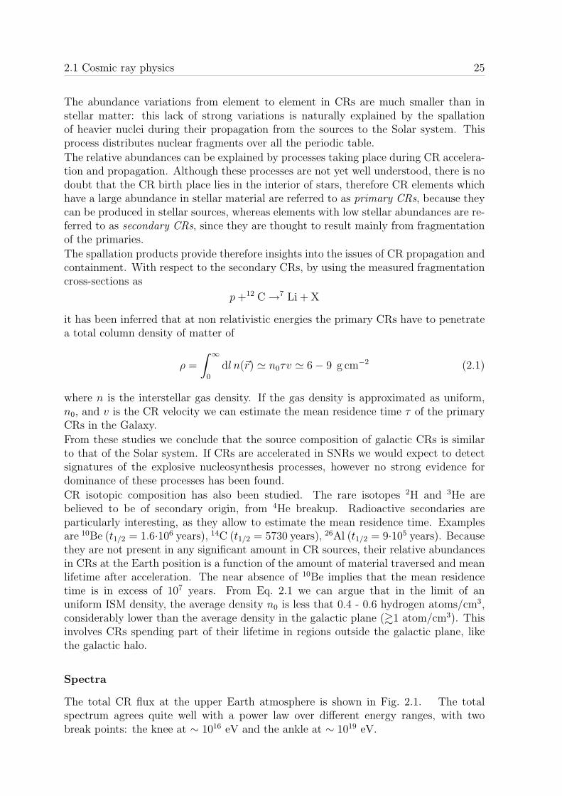
The total CR flux at the upper Earth atmosphere is shown in Fig. 2.1. The totalspectrum agrees quite well with a power law over different energy ranges, with twobreak points: the knee at ∼ 1016 eV and the ankle at ∼ 1019 eV.
26 Diffuse galactic gamma rays: a cosmic ray tracer
gested that the cosmic rays were the result of the forma-tion of complex nuclei from primary protons and elec-trons. In the 1920s electrons and ionized hydrogen werethe only known elementary particles to serve as buildingblocks for atomic nuclei. The formation of atomic nucleiwas assumed to be taking place throughout the universe,with the release of the binding energy in the form ofgamma radiation, which was the ‘‘cosmic radiation.’’ Aconsequence of this hypothesis was that the cosmic ra-diation was neutral and would not be influenced by theearth’s magnetic field. A worldwide survey led byArthur Compton demonstrated conclusively that the in-tensity of the cosmic radiation depended on the mag-netic latitude (Compton 1933). The cosmic radiation waspredominately charged particles. This result was thesubject of an acrimonious debate between Compton andMillikan at an AAAS meeting that made the front pageof the New York Times on December 31, 1932.
In 1938, Pierre Auger and Roland Maze, in their Parislaboratory, showed that cosmic-ray particles separatedby distances as large as 20 meters arrived in time coin-cidence (Auger and Maze, 1938), indicating that the ob-served particles were secondary particles from a com-mon source. Subsequent experiments in the Alpsshowed that the coincidences continued to be observedeven at a distance of 200 meters. This led Pierre Auger,in his 1939 article in Reviews of Modern Physics, to con-clude
One of the consequences of the extension of the en-ergy spectrum of cosmic rays up to 1015 eV is that itis actually impossible to imagine a single process ableto give to a particle such an energy. It seems muchmore likely that the charged particles which consti-tute the primary cosmic radiation acquire their en-ergy along electric fields of a very great extension.(Auger et al., 1939).
Auger and his colleagues discovered that there existedin nature particles with an energy of 1015 eV at a timewhen the largest energies from natural radioactivity orartificial acceleration were just a few MeV. Auger’samazement at Nature’s ability to produce particles ofenormous energies remains with us today, as there is noclear understanding of the mechanism of production,nor is there sufficient data available at present to hopeto draw any conclusions.
In 1962 John Linsley observed a cosmic ray whoseenergy was 1020 eV (Linsley, 1962). This event was ob-served by an array of scintillation counters spread over8 km2 in the desert near Albuquerque, New Mexico.The energetic primary was detected by sampling someof the 531010 particles produced by its cascade in theatmosphere. Linsley’s ground array was the first of anumber of large cosmic-ray detectors that have mea-sured the cosmic-ray spectrum at the highest energies.
III. COSMIC-RAY SPECTRUM
After 85 years of research, a great deal has beenlearned about the nature and sources of cosmic radia-
tion (Zatsepin et al., 1966; Berezinskii et al., 1990; Wat-son, 1991; Cronin, 1992; Sokolsky et al., 1992; Swordy,1994; Nagano, 1996; Yoshida et al., 1998). In Fig. 1 thespectrum of cosmic rays is plotted for energies above108 eV. The cosmic rays are predominately atomic nu-clei ranging in species from protons to iron nuclei, withtraces of heavier elements. When ionization potential istaken into account, as well as spallation in the residualgas of space, the relative abundances are similar to theabundances of elements found in the sun. The energiesrange from less than 1 MeV to more than 1020 eV. Thedifferential flux is described by a power law:
dN/dE;E2a, (3.1)
where the spectral index a is roughly 3, implying that theintensity of cosmic rays above a given energy decreasesby a factor of 100 for each decade in energy. The flux ofcosmic rays is about 1/cm2/sec at 100 MeV and only oforder 1/km2/century at 1020 eV.
The bulk of the cosmic rays are believed to have agalactic origin. The acceleration mechanism for thesecosmic rays is thought to be shock waves from super-nova explosions. This basic idea was first proposed byEnrico Fermi (1949), who discussed the acceleration ofcosmic rays as a process of the scattering of the chargedcosmic-ray particles off moving magnetic clouds. Subse-quent work has shown that multiple ‘‘bounces’’ off theturbulent magnetic fields associated with supernovashock waves is a more efficient acceleration process
FIG. 1. Spectrum of cosmic rays greater than 100 MeV. Thisfigure was produced by S. Swordy, University of Chicago.
S166 James W. Cronin: Cosmic rays
Rev. Mod. Phys., Vol. 71, No. 2, Centenary 1999
Figure 2.1: Total CR flux at the upper atmosphere [16].
Cosmic ray spectrum is bound at high energies by the CMB at 2.7 K, which destroysheavy nuclei with energies greater than ∼1019 eV/nucleon via photodisintegration
AX + γ →(A−1)X + n
and protons with energies greater than ∼1020 eV via pion photoproduction
p+ γ → p+ π0
There is also a low energy bound due to ionization energy losses, which increases rapidlywith decreasing particle energy.All component spectra are well represented by simple power law in kinetic energy pernucleon
dN
dE∝ Eγ
but the spectral index γ varies significantly from element to element. The Fe-groupenergy spectrum is the flattest, indicating a steady increase in the relative abundance ofIron with increasing energy. Moreover the measured decrease of the abundance ratio ofthe secondary nuclei with respect to their parents as B/C and N/O implies that particleswith higher energies traverse less interstellar matter than those with lower energies.
Directional distribution
The study of anisotropy in CR arrival direction is clearly of great interest to locate theirpossible sources. We could expect an anisotropy towards the galactic center direction
2.1 Cosmic ray physics 27
if CR sources were galactic objects due to the solar system position. However thereare big problems in interpreting data, due to experimental issues such as non uniformacceptance of CR detectors, sensitivity biases . . . By now data show no strong evidenceof anisotropy at any energy, regardless of the energy calibration chosen.In 1983 Samorski and Stamm [48] found possible directional anisotropies at energies ofabout 1015 eV. They found six possible directions where significant excesses of showersoccurred. One of them was the direction of the XRB Cyg X-3. Unfortunately Cyg X-3has not been detected as a γ-ray source, so we do not have a strong evidence for particleacceleration in this region.
2.1.3 CR interactions in the interstellar medium
Since direct measurements of cosmic ray particles are restricted to the near vicinity ofthe Earth, any information of cosmic radiation in more distant regions of space is basedon the detection of cosmic ray interaction products, such as electromagnetic radiation.As already told in 1.3.8, the galactic diffuse γ-rays prove that CRs are galactic in origin.Other clues from γ-astrophysics will be discussed in detail in 2.2.3. In this paragraphwe discuss the most important interaction processes.
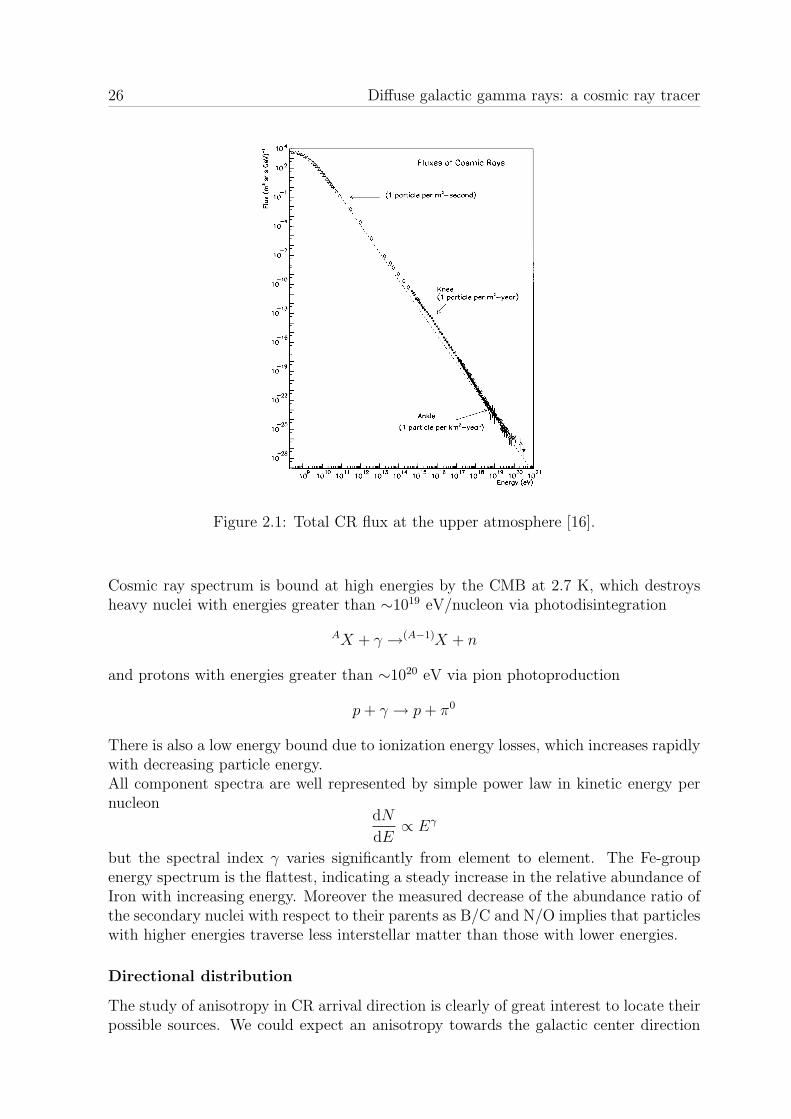
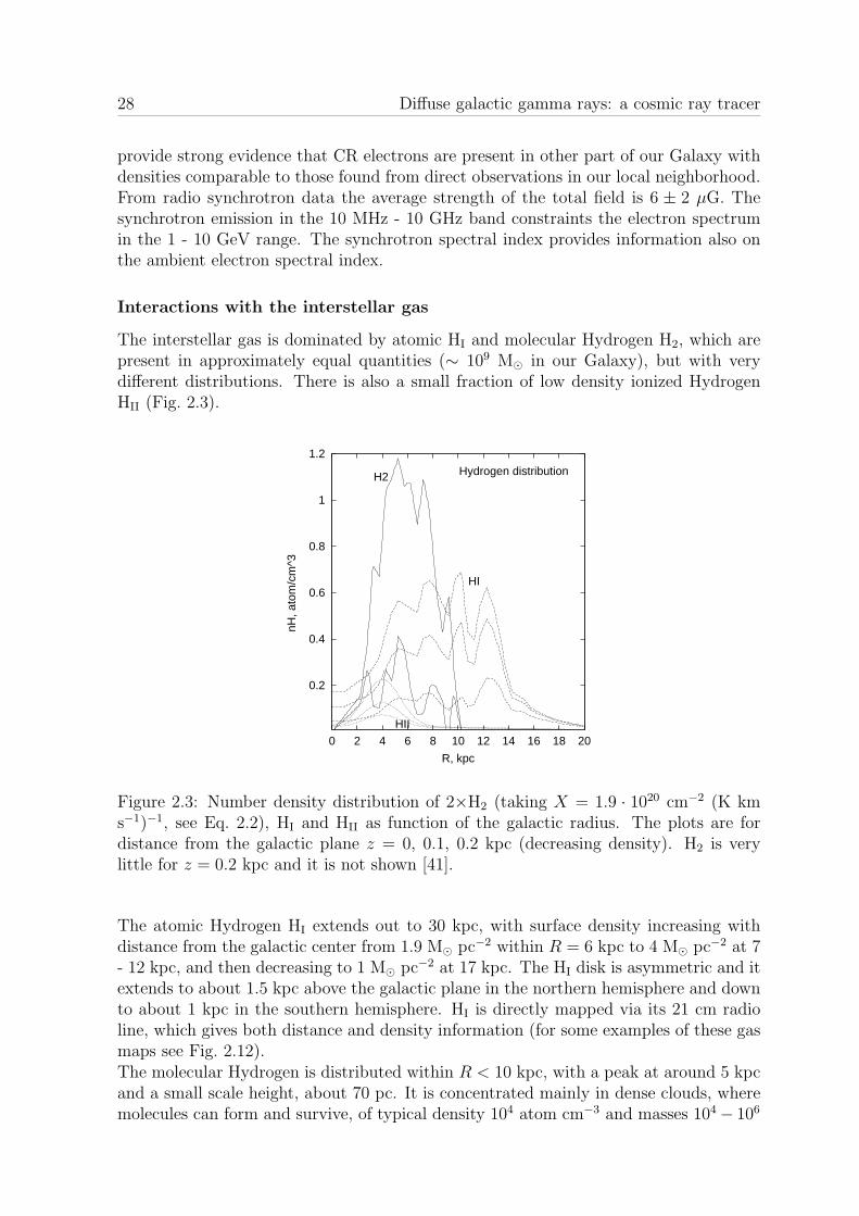
Interactions with the galactic magnetic field
The global structure of the Galactic magnetic field is currently derived from observationsof rotation measures of more than 500 pulsars. It is best described by two distinctcomponents (Fig. 2.2):
Figure 2.2: The antisymmetric field structure of the galactic halo [41].
1. a bi-symmetric spiral field in the disk with reversed direction from arm to arm;
2. an azimuthal field in the halo with reversed directions below and above the galacticplane.
Optical and synchrotron polarization data yield an average intensity of 4± 1 µG.Since relativistic electrons emit via synchrotron radiation in the surrounding magneticfields, radio-astronomy provides several clues about CRs. In particular, these surveys
28 Diffuse galactic gamma rays: a cosmic ray tracer
provide strong evidence that CR electrons are present in other part of our Galaxy withdensities comparable to those found from direct observations in our local neighborhood.From radio synchrotron data the average strength of the total field is 6 ± 2 µG. Thesynchrotron emission in the 10 MHz - 10 GHz band constraints the electron spectrumin the 1 - 10 GeV range. The synchrotron spectral index provides information also onthe ambient electron spectral index.
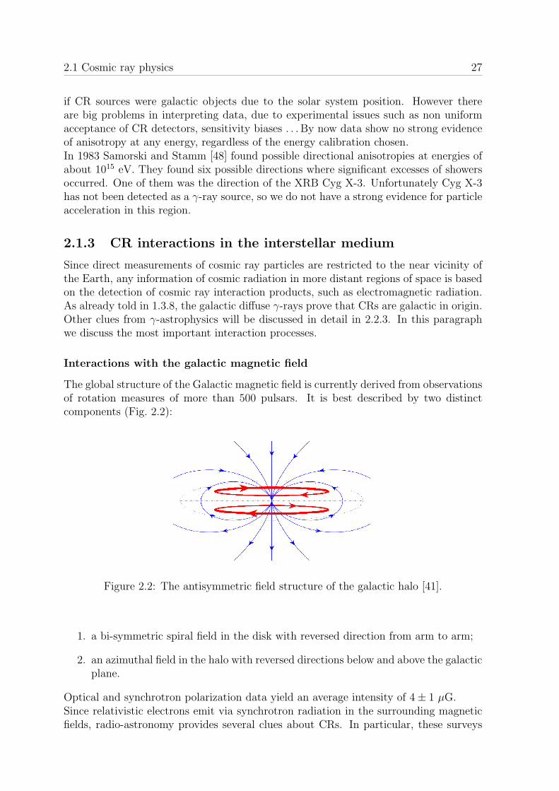
Interactions with the interstellar gas
The interstellar gas is dominated by atomic HI and molecular Hydrogen H2, which arepresent in approximately equal quantities (∼ 109 M in our Galaxy), but with verydifferent distributions. There is also a small fraction of low density ionized HydrogenHII (Fig. 2.3).
0.2
0.4
0.6
0.8
1
1.2
0 2 4 6 8 10 12 14 16 18 20
nH, a
tom
/cm
^3
R, kpc
Hydrogen distributionH2
HI
HII
Figure 2.3: Number density distribution of 2×H2 (taking X = 1.9 · 1020 cm−2 (K kms−1)−1, see Eq. 2.2), HI and HII as function of the galactic radius. The plots are fordistance from the galactic plane z = 0, 0.1, 0.2 kpc (decreasing density). H2 is verylittle for z = 0.2 kpc and it is not shown [41].
The atomic Hydrogen HI extends out to 30 kpc, with surface density increasing withdistance from the galactic center from 1.9 M pc−2 within R = 6 kpc to 4 M pc−2 at 7- 12 kpc, and then decreasing to 1 M pc−2 at 17 kpc. The HI disk is asymmetric and itextends to about 1.5 kpc above the galactic plane in the northern hemisphere and downto about 1 kpc in the southern hemisphere. HI is directly mapped via its 21 cm radioline, which gives both distance and density information (for some examples of these gasmaps see Fig. 2.12).The molecular Hydrogen is distributed within R < 10 kpc, with a peak at around 5 kpcand a small scale height, about 70 pc. It is concentrated mainly in dense clouds, wheremolecules can form and survive, of typical density 104 atom cm−3 and masses 104− 106
2.2 GALPROP models 29
M. The H2 gas cannot be detected directly on large scale, but we can use the CO lineat 2.6 mm (corresponding to the J = 1 → 0 rotational transition) as H2 tracer, sinceCarbon monoxide resides in the dense clouds mainly composed by H2. All molecularclouds show CO emission so, since the 1970s, the easily observable 2.6 mm line of COhas become a valuable tool in the study of the highly condensed parts of the interstellarmedium. The derivation of H2 density from CO data is still problematic. From 2.6 mmCO surveys we can measure the peak line radiation temperature TR and the integratedradiation temperature (K km s−1)
WCO =
∫TR dv
The simplest solution is to assume that the Hydrogen column density NH2 (cm−2) alongthe line of sight in a certain direction is locally proportional to the integrated tempera-ture of the CO emission WCO
NH2 = X ·WCO (2.2)
as found by Kutner and Leung [32]. The last complete CO survey from Dame et al. [17]yields an average value X = 1.8 · 1020 cm−2 (K km s−1)−1.
CR electrons can interact with the interstellar gas via nonthermal bremsstrahlung pro-ducing γ-rays. CR electrons can also loose energy ionizing or exciting atoms andmolecules of the ISM. CR nuclei interact with the gas via bremsstrahlung and inelasticcollisions, producing in both cases γ-rays.
Interactions with the interstellar radiation field
The interstellar radiation field is made up of contributions from starlight, emissionfrom dust and the CMB. New data from the IRAS and COBE (COsmic BackgroundExplorer) satellites have greatly improved our knowledge of both the stellar distributionand the dust emission. Fig. 2.4 shows on the left ISRF energy density as function ofthe galactocentric radius and on the right a recent estimate of the spectrum at 8 kpc,near the Sun position. The ISRF has a vertical extent of several kpc and the radialdistribution of the stellar component is centrally peaked.
CR electrons interact with the ISRF via ICS producing γ-rays. Both CR nuclei andelectrons interact with the ISRF via photo-pair production, other processes leading toγ-ray production.
2.2 GALPROP models
A numerical method and corresponding computer code for the calculation of galacticCR propagation was developed by A. W. Strong and I. V. Moskalenko. The modelsimultaneously reproduces observational data of many kinds: direct detection of CRand indirect observations via γ-rays and synchrotron radiation.

30 Diffuse galactic gamma rays: a cosmic ray tracer
Figure 2.4: On the left: ISRF energy density as function of the galactic radius R in thegalactic plane. On the right: spectrum of the ISRF at the Sun position [41].
2.2.1 The GALPROP code
The transport equation
The GALPROP code [57] solves the transport equation (see appendix A) for all CRspecies given the source distribution and the boundary conditions . This equationincludes diffusion, convection, diffusive reacceleration in the ISM, energy losses, nuclearfragmentation and decay. The spatial boundary conditions assume free particle escape.The solution can be 3-dimensional (cylindrical) (R, z, p) or 4-dimensional (x, y, z, p)(spatial variables plus momentum). The transport Eq. A.1 is rewritten in the form
∂ψ
∂t= q(~r, p) +∇ ·
(Dxx
~∇ψ − ~V ψ)
+∂
∂pp2Dpp
∂
∂p
1
p2ψ +
− ∂
∂p
[pψ − p
3
(∇ · ~V
)ψ
]− 1
τfψ − 1
τrψ (2.3)
where ψ(~r, p, t) is the density function of total particle momentum, ψ(p)dp = 4πp2f(~p)dpif f(~p) is the distribution function of the species. On the right side q(~r, p) is the dis-
tribution of CR sources, Dxx is the spatial diffusion coefficient and ~V is the convectionvelocity (Eq. A.1)
~V = ~U +1
4p2
∂
∂p(p2~vA1)
Reacceleration is described as diffusion in momentum space determined by the coeffi-cient Dpp, p is the momentum loss rate, τf the meantime for fragmentation and τr themeantime for radioactive decay.For a given halo size the diffusion coefficient as a function of momentum and the reaccel-eration or convection parameters are determined by B to C ratio data (see below 2.2.2).

2.2 GALPROP models 31
The spatial diffusion coefficient is taken as
Dxx =
βD0(R/R0)
δ1 R ≤ R0
βD0(R/R0)δ2 R > R0
(2.4)
where R is rigidity and β = (v/c) is a consequence of random walk process. Usuallyδ1 = δ2 = δ is taken 1/3. For the reacceleration the momentum-space diffusion coefficientDpp is related to the spatial coefficient Dxx (this equation is derived in [49], [52])
Dpp ·Dxx =4p2v2
A
3δ(4− δ2)(4− δ)w(2.5)
where the main free parameter is the Alfven speed vA and w characterizes the level ofturbulence. Only the ratio v2
A/w is physically relevant, so GALPROP takes w = 1. Theconvection velocity V (z) is assumed to increase linearly with distance from the galacticplane.The distribution of CR sources is chosen such to reproduce the distribution determinedby analysis of EGRET γ-ray data
q(R, z) = q0
(R
R
)η
exp
(−ξ R−R
R− |z|
0.2 kpc
)The z-dependence reflects the assumed confinement to the disk. The R-dependence hasthe same parametrization as that used for SNRs, but with different parameters in orderto fit γ-ray data. However, the galactic distribution of SNRs, commonly based on radiosurveys, is subject to large observational selection effects. Other tracers are available, inparticular pulsars. This topic will be discussed below (see 2.2.3). A cutoff in the sourcedistribution is applied at R = 20 kpc, since it is unlikely that significant sources arepresent at such large radii. For reasons explained at the end of appendix A, the injectionspectrum of nucleons and electrons is assumed to be a power law in momentum
dq
dp(p) ∝ pγ
Energy losses for nucleons by ionization and Coulomb interactions are included, andfor electrons by ionization, Coulomb interactions, bremsstrahlung, ICS (in isotropicapproximation) and synchrotron emission.At the beginning the primary propagation is computed as a function of (R, z, p); thenthe secondary source function is obtained from the gas density and cross sections, andthe secondary propagation is computed. Finally tertiary reactions such as 11B → 10Bare treated.
Inputs from astrophysical observations
GALPROP models, as well as theoretical developments about the CR transport equa-tion, use realistic physical and astrophysical inputs. The galactic halo is described by acylindrical model, with radius R < 30 kpc and height z = 1÷20 kpc. The distance fromthe Sun to the galactic center is taken as 8.5 kpc. The total magnetic field distributionis adjusted to match the 408 MHz synchrotron longitude and latitude distributions
B = B0 exp
(−R−R
RB
− |z|zB
)
32 Diffuse galactic gamma rays: a cosmic ray tracer
in agreement with the model by Vallee [60].The interstellar Hydrogen distribution uses radio surveys data (see 2.1.3). The Heliumnumerical fraction is taken as 0.11, according to a wide range of observations. For γ-rayskymaps calculation the WCO intensity is defined in the form of tables in 9 galactocentricrings, using the standard Dame survey [17], and the conversion factor X from CO to H2
can be different in each ring; tables with HI number density in 9 galactocentric rings arecalculated from the Gordon and Burton data [26]. To solve the transport equation inthe current release GALPROP uses an analytical cylindrical model of gas distributionobtained from these tables and assuming a constant value of X = 1.9 · 1020 cm−2 (K kms−1)−1, but improvements are on the way.The HII distribution is described by the Cordes function [15]
nHII= 0.025 exp
[− |z|
1 kpc−
(R
20 kpc
)2]
+ 0.2 exp
[− |z|
0.15 kpc−
(R
2 kpc− 2
)2]
cm−3
where the first term represents the extensive warm ionized gas, while the second onerepresents HII regions and is concentrated around R = 4 kpc.The ISRF is described by an up to date model by Porter and Strong [44]. It features amodel for the distribution of stars in the Galaxy developed by Wainscoat [62], improvedto include the recently discovered offset bar, the cutoff in stellar counts at about 3 kpcobserved by COBE and new data about stellar spectra. It includes absorption andemission in IR from interstellar dust, and obviously the CMB as observed by COBE.The program uses the cross-section measurements and spectrum fitting from the LANLNuclear Data Sheets, collecting results from experiments carried out from 1969 to 1999.In particular, evaluation of production cross sections of light elements (Li, Be, B) isimportant for models of CR propagation. Predictions of nuclear codes have been testedagainst isobaric and cumulative data where available [40].
2.2.2 Constraints from CR direct observations
Direct CR observations provide several constraints on GALPROP models. The modelshave been compared with CR data from HEAO 3, Voyager 1 and 2 and Ulysses.The main clue is the presence of the reacceleration mechanism, which provides a naturalexplanation for the energy dependence of the Boron over Carbon ratio. The B/C ratiois used because it is the most accurately measured ratio covering a wide energy rangeand the cross-section
p+12 C →8 B + X
is well established. Simple diffusion/convection models have difficulty in accounting forthe observed form of the B/C ratio without specific assumptions to fit data and on thediffusion coefficient. Otherwise, models with reacceleration account naturally for theenergy dependence over the whole observed range (Fig. 2.5). These data give a valuefor the Alfven velocity of vA ≈ 20 km/s.Furthermore, a very sensitive quantity is the ratio 10Be/9Be, not strongly dependenton solar modulation, which gives a halo height from 4 to 20 kpc for a model includingreacceleration (Fig. 2.6).The positron fraction given by models with reacceleration is consistent with measure-ments up to 10 GeV, beyond which some excess is apparent. The electron spectrum for
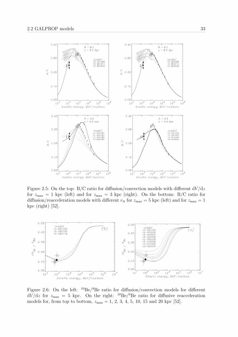
2.2 GALPROP models 33
Figure 2.5: On the top: B/C ratio for diffusion/convection models with different dV/dzfor zmax = 1 kpc (left) and for zmax = 3 kpc (right). On the bottom: B/C ratio fordiffusion/reacceleration models with different vA for zmax = 5 kpc (left) and for zmax = 1kpc (right) [52].
Figure 2.6: On the left: 10Be/9Be ratio for diffusion/convection models for differentdV/dz for zmax = 5 kpc. On the right: 10Be/9Be ratio for diffusive reaccelerationmodels for, from top to bottom, zmax = 1, 2, 3, 4, 5, 10, 15 and 20 kpc [52].
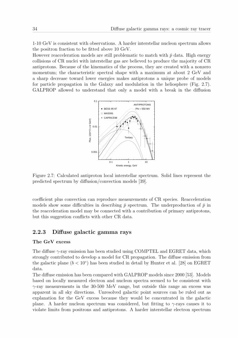
34 Diffuse galactic gamma rays: a cosmic ray tracer
1-10 GeV is consistent with observations. A harder interstellar nucleon spectrum allowsthe positron fraction to be fitted above 10 GeV.
However reacceleration models are still problematic to match with p data. High energycollisions of CR nuclei with interstellar gas are believed to produce the majority of CRantiprotons. Because of the kinematics of the process, they are created with a nonzeromomentum; the characteristic spectral shape with a maximum at about 2 GeV anda sharp decrease toward lower energies makes antiprotons a unique probe of modelsfor particle propagation in the Galaxy and modulation in the heliosphere (Fig. 2.7).GALPROP allowed to understand that only a model with a break in the diffusion
0.001
0.01
0.1
0.1 1 10
Flu
x, 1
/(m
^2 s
sr
GeV
)
Kinetic energy, GeV
ANTIPROTONS
Phi = 550 MVBESS 95-97
MASS91
CAPRICE98
Tertiary
Figure 2.7: Calculated antiproton local interstellar spectrum. Solid lines represent thepredicted spectrum by diffusion/convection models [39].
coefficient plus convection can reproduce measurements of CR species. Reaccelerationmodels show some difficulties in describing p spectrum. The underproduction of p inthe reacceleration model may be connected with a contribution of primary antiprotons,but this suggestion conflicts with other CR data.
2.2.3 Diffuse galactic gamma rays
The GeV excess
The diffuse γ-ray emission has been studied using COMPTEL and EGRET data, whichstrongly contributed to develop a model for CR propagation. The diffuse emission fromthe galactic plane (b < 10) has been studied in detail by Hunter et al. [28] on EGRETdata.
The diffuse emission has been compared with GALPROP models since 2000 [53]. Modelsbased on locally measured electron and nucleon spectra seemed to be consistent withγ-ray measurements in the 30-500 MeV range, but outside this range an excess wasapparent in all sky directions. Unresolved galactic point sources can be ruled out asexplanation for the GeV excess because they would be concentrated in the galacticplane. A harder nucleon spectrum was considered, but fitting to γ-rays causes it toviolate limits from positrons and antiprotons. A harder interstellar electron spectrum
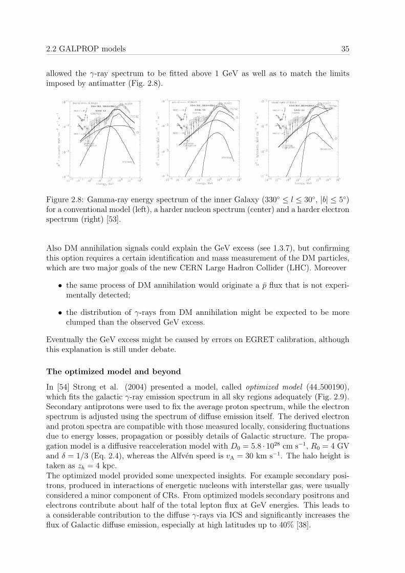
2.2 GALPROP models 35
allowed the γ-ray spectrum to be fitted above 1 GeV as well as to match the limitsimposed by antimatter (Fig. 2.8).
0.5<l< 30.0 , 330.0<l<359.0
-5.0<b< 5.0
0.5<l< 30.0 , 330.0<l<359.0
-5.0<b< 5.0
0.5<l< 30.0 , 330.0<l<359.0
-5.0<b< 5.0
Figure 2.8: Gamma-ray energy spectrum of the inner Galaxy (330 ≤ l ≤ 30, |b| ≤ 5)for a conventional model (left), a harder nucleon spectrum (center) and a harder electronspectrum (right) [53].
Also DM annihilation signals could explain the GeV excess (see 1.3.7), but confirmingthis option requires a certain identification and mass measurement of the DM particles,which are two major goals of the new CERN Large Hadron Collider (LHC). Moreover
• the same process of DM annihilation would originate a p flux that is not experi-mentally detected;
• the distribution of γ-rays from DM annihilation might be expected to be moreclumped than the observed GeV excess.
Eventually the GeV excess might be caused by errors on EGRET calibration, althoughthis explanation is still under debate.
The optimized model and beyond
In [54] Strong et al. (2004) presented a model, called optimized model (44 500190),which fits the galactic γ-ray emission spectrum in all sky regions adequately (Fig. 2.9).Secondary antiprotons were used to fix the average proton spectrum, while the electronspectrum is adjusted using the spectrum of diffuse emission itself. The derived electronand proton spectra are compatible with those measured locally, considering fluctuationsdue to energy losses, propagation or possibly details of Galactic structure. The propa-gation model is a diffusive reacceleration model with D0 = 5.8 · 1028 cm s−1, R0 = 4 GVand δ = 1/3 (Eq. 2.4), whereas the Alfven speed is vA = 30 km s−1. The halo height istaken as zh = 4 kpc.The optimized model provided some unexpected insights. For example secondary posi-trons, produced in interactions of energetic nucleons with interstellar gas, were usuallyconsidered a minor component of CRs. From optimized models secondary positrons andelectrons contribute about half of the total lepton flux at GeV energies. This leads toa considerable contribution to the diffuse γ-rays via ICS and significantly increases theflux of Galactic diffuse emission, especially at high latitudes up to 40% [38].
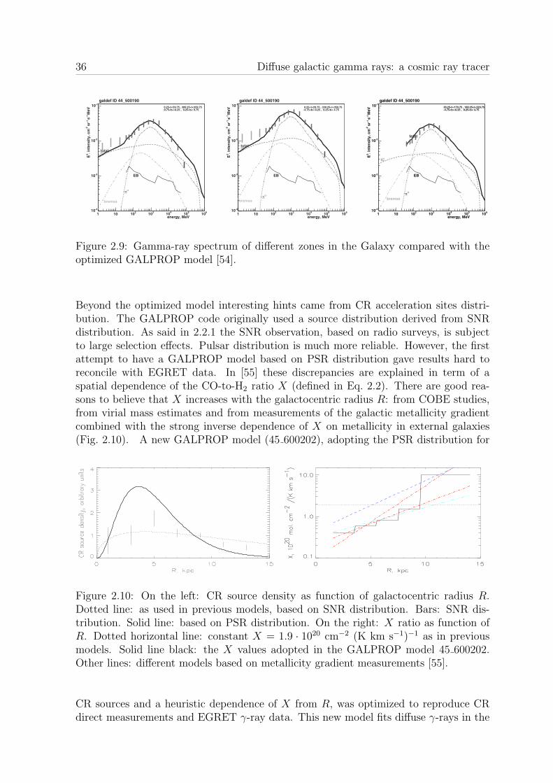
36 Diffuse galactic gamma rays: a cosmic ray tracer
Figure 2.9: Gamma-ray spectrum of different zones in the Galaxy compared with theoptimized GALPROP model [54].
Beyond the optimized model interesting hints came from CR acceleration sites distri-bution. The GALPROP code originally used a source distribution derived from SNRdistribution. As said in 2.2.1 the SNR observation, based on radio surveys, is subjectto large selection effects. Pulsar distribution is much more reliable. However, the firstattempt to have a GALPROP model based on PSR distribution gave results hard toreconcile with EGRET data. In [55] these discrepancies are explained in term of aspatial dependence of the CO-to-H2 ratio X (defined in Eq. 2.2). There are good rea-sons to believe that X increases with the galactocentric radius R: from COBE studies,from virial mass estimates and from measurements of the galactic metallicity gradientcombined with the strong inverse dependence of X on metallicity in external galaxies(Fig. 2.10). A new GALPROP model (45 600202), adopting the PSR distribution for
Figure 2.10: On the left: CR source density as function of galactocentric radius R.Dotted line: as used in previous models, based on SNR distribution. Bars: SNR dis-tribution. Solid line: based on PSR distribution. On the right: X ratio as function ofR. Dotted horizontal line: constant X = 1.9 · 1020 cm−2 (K km s−1)−1 as in previousmodels. Solid line black: the X values adopted in the GALPROP model 45 600202.Other lines: different models based on metallicity gradient measurements [55].
CR sources and a heuristic dependence of X from R, was optimized to reproduce CRdirect measurements and EGRET γ-ray data. This new model fits diffuse γ-rays in the
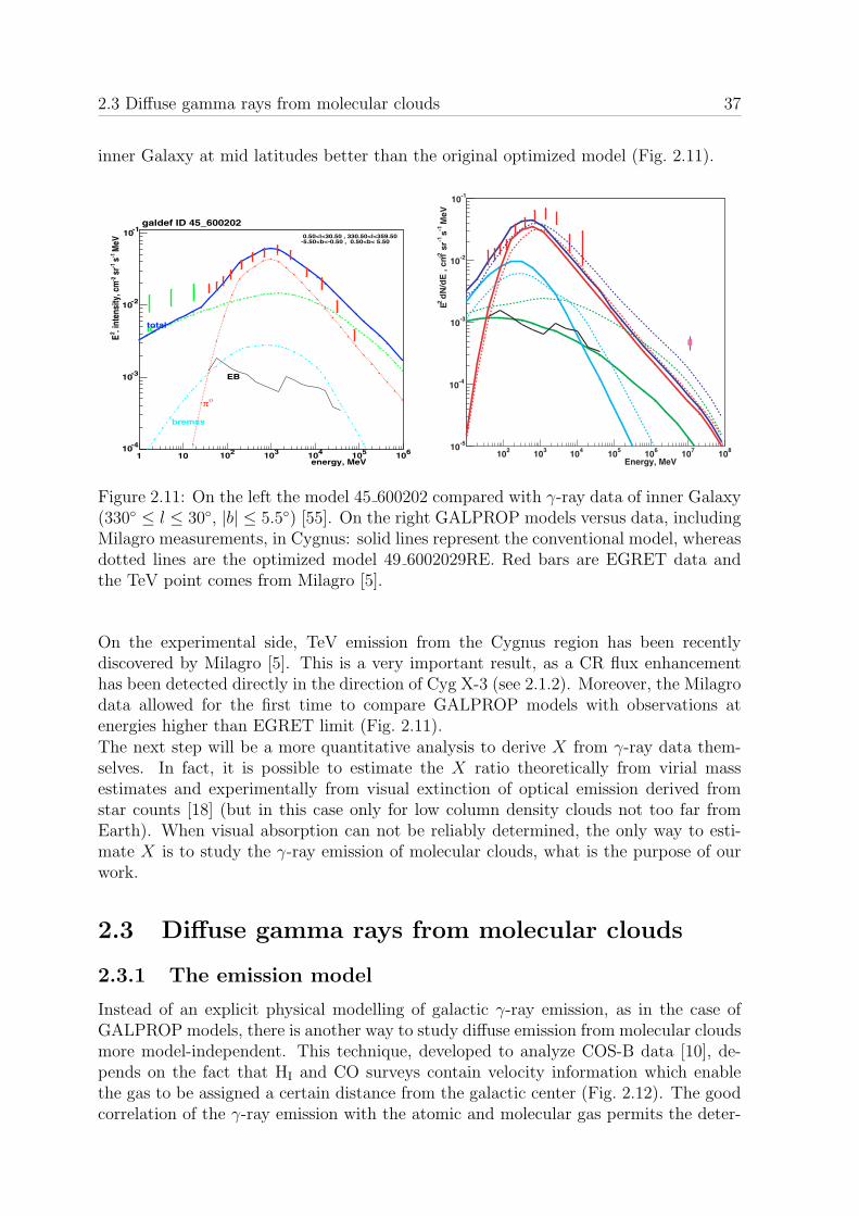
2.3 Diffuse gamma rays from molecular clouds 37
inner Galaxy at mid latitudes better than the original optimized model (Fig. 2.11).
energy, MeV1 10 210 310 410 510 610
MeV
-1 s
-1 s
r-2
. int
ensi
ty, c
m2 E
-410
-310
-210
-110 galdef ID 45_600202
0.50<l<30.50 , 330.50<l<359.50 -5.50<b<-0.50 , 0.50<b< 5.50
IC
bremss
πο
total
EB
Figure 2.11: On the left the model 45 600202 compared with γ-ray data of inner Galaxy(330 ≤ l ≤ 30, |b| ≤ 5.5) [55]. On the right GALPROP models versus data, includingMilagro measurements, in Cygnus: solid lines represent the conventional model, whereasdotted lines are the optimized model 49 6002029RE. Red bars are EGRET data andthe TeV point comes from Milagro [5].
On the experimental side, TeV emission from the Cygnus region has been recentlydiscovered by Milagro [5]. This is a very important result, as a CR flux enhancementhas been detected directly in the direction of Cyg X-3 (see 2.1.2). Moreover, the Milagrodata allowed for the first time to compare GALPROP models with observations atenergies higher than EGRET limit (Fig. 2.11).The next step will be a more quantitative analysis to derive X from γ-ray data them-selves. In fact, it is possible to estimate the X ratio theoretically from virial massestimates and experimentally from visual extinction of optical emission derived fromstar counts [18] (but in this case only for low column density clouds not too far fromEarth). When visual absorption can not be reliably determined, the only way to esti-mate X is to study the γ-ray emission of molecular clouds, what is the purpose of ourwork.
2.3 Diffuse gamma rays from molecular clouds
2.3.1 The emission model
Instead of an explicit physical modelling of galactic γ-ray emission, as in the case ofGALPROP models, there is another way to study diffuse emission from molecular cloudsmore model-independent. This technique, developed to analyze COS-B data [10], de-pends on the fact that HI and CO surveys contain velocity information which enablethe gas to be assigned a certain distance from the galactic center (Fig. 2.12). The goodcorrelation of the γ-ray emission with the atomic and molecular gas permits the deter-
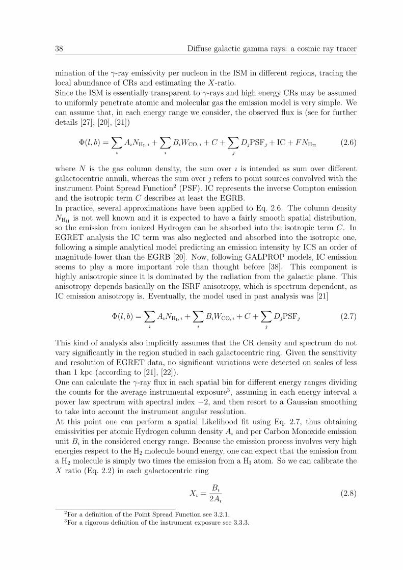
38 Diffuse galactic gamma rays: a cosmic ray tracer
mination of the γ-ray emissivity per nucleon in the ISM in different regions, tracing thelocal abundance of CRs and estimating the X-ratio.Since the ISM is essentially transparent to γ-rays and high energy CRs may be assumedto uniformly penetrate atomic and molecular gas the emission model is very simple. Wecan assume that, in each energy range we consider, the observed flux is (see for furtherdetails [27], [20], [21])
Φ(l, b) =∑
ı
AıNHI, ı +∑
ı
BıWCO, ı + C +∑
DPSF + IC + FNHII(2.6)
where N is the gas column density, the sum over ı is intended as sum over differentgalactocentric annuli, whereas the sum over refers to point sources convolved with theinstrument Point Spread Function2 (PSF). IC represents the inverse Compton emissionand the isotropic term C describes at least the EGRB.In practice, several approximations have been applied to Eq. 2.6. The column densityNHII
is not well known and it is expected to have a fairly smooth spatial distribution,so the emission from ionized Hydrogen can be absorbed into the isotropic term C. InEGRET analysis the IC term was also neglected and absorbed into the isotropic one,following a simple analytical model predicting an emission intensity by ICS an order ofmagnitude lower than the EGRB [20]. Now, following GALPROP models, IC emissionseems to play a more important role than thought before [38]. This component ishighly anisotropic since it is dominated by the radiation from the galactic plane. Thisanisotropy depends basically on the ISRF anisotropy, which is spectrum dependent, asIC emission anisotropy is. Eventually, the model used in past analysis was [21]
Φ(l, b) =∑
ı
AıNHI, ı +∑
ı
BıWCO, ı + C +∑
DPSF (2.7)
This kind of analysis also implicitly assumes that the CR density and spectrum do notvary significantly in the region studied in each galactocentric ring. Given the sensitivityand resolution of EGRET data, no significant variations were detected on scales of lessthan 1 kpc (according to [21], [22]).One can calculate the γ-ray flux in each spatial bin for different energy ranges dividingthe counts for the average instrumental exposure3, assuming in each energy interval apower law spectrum with spectral index −2, and then resort to a Gaussian smoothingto take into account the instrument angular resolution.At this point one can perform a spatial Likelihood fit using Eq. 2.7, thus obtainingemissivities per atomic Hydrogen column density Aı and per Carbon Monoxide emissionunit Bı in the considered energy range. Because the emission process involves very highenergies respect to the H2 molecule bound energy, one can expect that the emission froma H2 molecule is simply two times the emission from a HI atom. So we can calibrate theX ratio (Eq. 2.2) in each galactocentric ring
Xı =Bı
2Aı
(2.8)
2For a definition of the Point Spread Function see 3.2.1.3For a rigorous definition of the instrument exposure see 3.3.3.
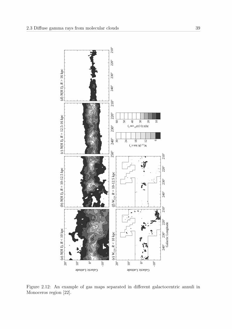
2.3 Diffuse gamma rays from molecular clouds 39
250240
230220
210
-10°0°10°
20°
Galactic Latitude(a
)N
(H I
), R
< 1
0 kp
c
-10°0°10°20°
(b)
N(H
I),
R =
10-
12.5
kpc
250°
240°
230°
220°
210°
-10°0°10°20°
(c)
N(H
I),
R =
12.
5-16
kpc
240°
230°
220°
210°
-10°0°10°20°
(d)
N(H
I),
R >
16
kpc
240°
230°
220°
210°
Gal
actic
Lon
gitu
de
-10°0°10°
20°
Galactic Latitude
(e)
WC
O,R
< 1
0 kp
c
240°
230°
220°
210°
-10°0°10°20°
(f)
WC
O,R
= 1
0-12
.5 k
pc
612182430
WCO (K km s-1
)
102030405060
N(H I) (1020
cm-2
)
Figure 2.12: An example of gas maps separated in different galactocentric annuli inMonoceros region [22].

40 Diffuse galactic gamma rays: a cosmic ray tracer
This X value is strictly speaking only a lower limit to the true value, because CRs couldbe excluded from the densest parts of the molecular clouds. This exclusion would beenergy dependent, however no energy dependence of the X-ratio has been indicated byfits of separate energy ranges on EGRET data.Diffuse γ-rays have been studied on EGRET data using this technique in four differentregions: Ophiucus, [27], Orion, [20], Cepheus and Polaris flares, [21], and Monoceros,[22]. A very important result is that emissivity is enhanced within Galaxy arms: thisprofile suggests an enhancement of CR density, especially protons, in arm regions. Thisfinding is consistent with the concept of coupling of gas and CRs, perhaps through theassociation of CR sources with interstellar gas and confinement of CRs by magneticfields associated with the gas.
2.3.2 X-ratio calibration
As told in 2.2.3, analysis of metal distribution and virial mass estimates strongly suggestthat X increases in the outer Galaxy and may have a fairly strong gradient at the Solarcircle. Virial estimates give an average value over the whole Galaxy of 1.9 · 1020 cm−2
(K km s−1)−1. The visual extinction of star counts allows to estimate X just in a fewcases for low density clouds on the galactic plane and not too far from the solar circle(otherwise this technique can not be used) [18].The aforementioned analysis technique (see 2.3.1) applied on EGRET data yielded theresults in Table 2.1.
R Xkpc 1020 cm−2 (K km s−1)−1
Ophiucus 8.4 1.1± 0.2Cepheus 8.7 0.92± 0.14Orion 8.9 1.35± 0.15Monoceros 9.2 1.64± 0.31
Table 2.1: X-ratio values on the local arm from EGRET data analysis in four differentregions [22].
Analysis of EGRET data looking for gradients in the values of X in the outer Galaxyhave been inconclusive, owing to the decreasing fraction of molecular gas and the modestangular resolution of EGRET. The only acceptable estimate comes from analysis ofCepheus region [21]: it yields an X-value on the Perseus arm of (2.48 ± 0.89) · 1020
cm−2 (K km s−1)−1 (40% error). The LAT, with its better effective area and angularresolution (Table 1.1), might strongly contribute to X-ratio calibration, allowing a greatimprovement in the models for the galactic diffuse emission and the knowledge of CRsources (see 2.2.3).
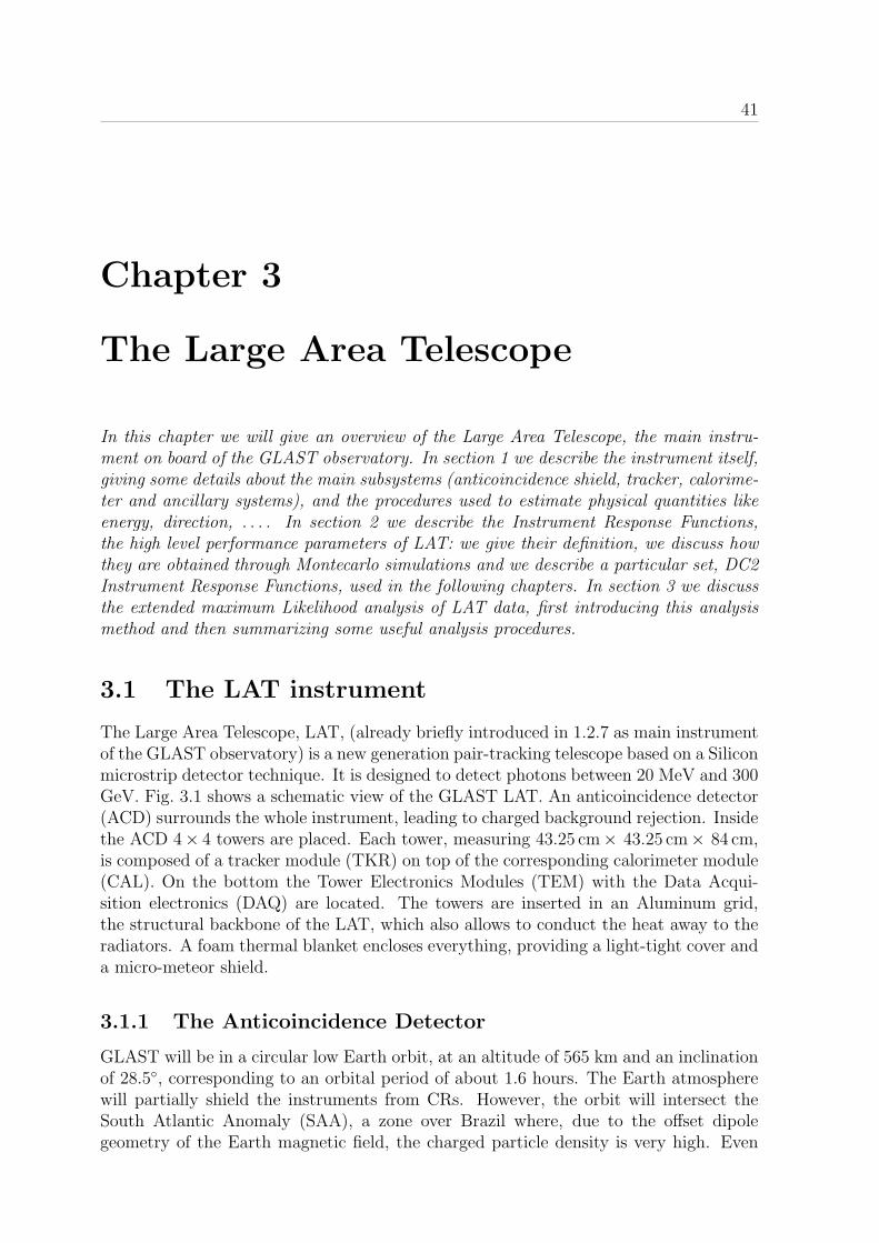
41
Chapter 3
The Large Area Telescope
In this chapter we will give an overview of the Large Area Telescope, the main instru-ment on board of the GLAST observatory. In section 1 we describe the instrument itself,giving some details about the main subsystems (anticoincidence shield, tracker, calorime-ter and ancillary systems), and the procedures used to estimate physical quantities likeenergy, direction, . . . . In section 2 we describe the Instrument Response Functions,the high level performance parameters of LAT: we give their definition, we discuss howthey are obtained through Montecarlo simulations and we describe a particular set, DC2Instrument Response Functions, used in the following chapters. In section 3 we discussthe extended maximum Likelihood analysis of LAT data, first introducing this analysismethod and then summarizing some useful analysis procedures.
3.1 The LAT instrument
The Large Area Telescope, LAT, (already briefly introduced in 1.2.7 as main instrumentof the GLAST observatory) is a new generation pair-tracking telescope based on a Siliconmicrostrip detector technique. It is designed to detect photons between 20 MeV and 300GeV. Fig. 3.1 shows a schematic view of the GLAST LAT. An anticoincidence detector(ACD) surrounds the whole instrument, leading to charged background rejection. Insidethe ACD 4× 4 towers are placed. Each tower, measuring 43.25 cm× 43.25 cm× 84 cm,is composed of a tracker module (TKR) on top of the corresponding calorimeter module(CAL). On the bottom the Tower Electronics Modules (TEM) with the Data Acqui-sition electronics (DAQ) are located. The towers are inserted in an Aluminum grid,the structural backbone of the LAT, which also allows to conduct the heat away to theradiators. A foam thermal blanket encloses everything, providing a light-tight cover anda micro-meteor shield.
3.1.1 The Anticoincidence Detector
GLAST will be in a circular low Earth orbit, at an altitude of 565 km and an inclinationof 28.5, corresponding to an orbital period of about 1.6 hours. The Earth atmospherewill partially shield the instruments from CRs. However, the orbit will intersect theSouth Atlantic Anomaly (SAA), a zone over Brazil where, due to the offset dipolegeometry of the Earth magnetic field, the charged particle density is very high. Even
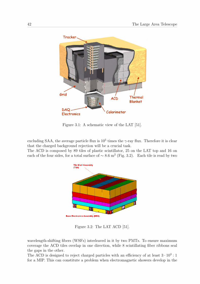
42 The Large Area Telescope
Figure 3.1: A schematic view of the LAT [51].
excluding SAA, the average particle flux is 105 times the γ-ray flux. Therefore it is clearthat the charged background rejection will be a crucial task.The ACD is composed by 89 tiles of plastic scintillator, 25 on the LAT top and 16 oneach of the four sides, for a total surface of ∼ 8.6 m2 (Fig. 3.2). Each tile is read by two
Figure 3.2: The LAT ACD [51].
wavelength-shifting fibers (WSFs) interleaved in it by two PMTs. To ensure maximumcoverage the ACD tiles overlap in one direction, while 8 scintillating fiber ribbons sealthe gaps in the other.The ACD is designed to reject charged particles with an efficiency of at least 3 · 103 : 1for a MIP. This can constitute a problem when electromagnetic showers develop in the
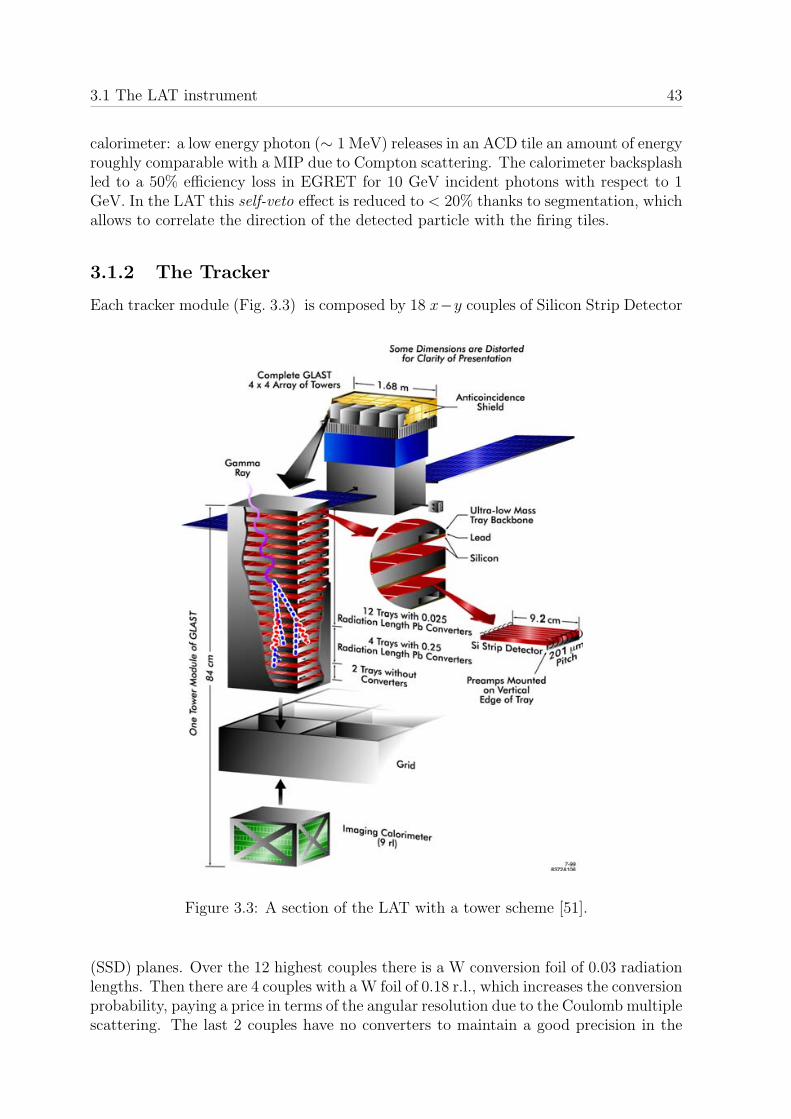
3.1 The LAT instrument 43
calorimeter: a low energy photon (∼ 1 MeV) releases in an ACD tile an amount of energyroughly comparable with a MIP due to Compton scattering. The calorimeter backsplashled to a 50% efficiency loss in EGRET for 10 GeV incident photons with respect to 1GeV. In the LAT this self-veto effect is reduced to < 20% thanks to segmentation, whichallows to correlate the direction of the detected particle with the firing tiles.
3.1.2 The Tracker
Each tracker module (Fig. 3.3) is composed by 18 x−y couples of Silicon Strip Detector
isd,nn
42
tafrf
s,
Figure 3.3: A section of the LAT with a tower scheme [51].
(SSD) planes. Over the 12 highest couples there is a W conversion foil of 0.03 radiationlengths. Then there are 4 couples with a W foil of 0.18 r.l., which increases the conversionprobability, paying a price in terms of the angular resolution due to the Coulomb multiplescattering. The last 2 couples have no converters to maintain a good precision in the
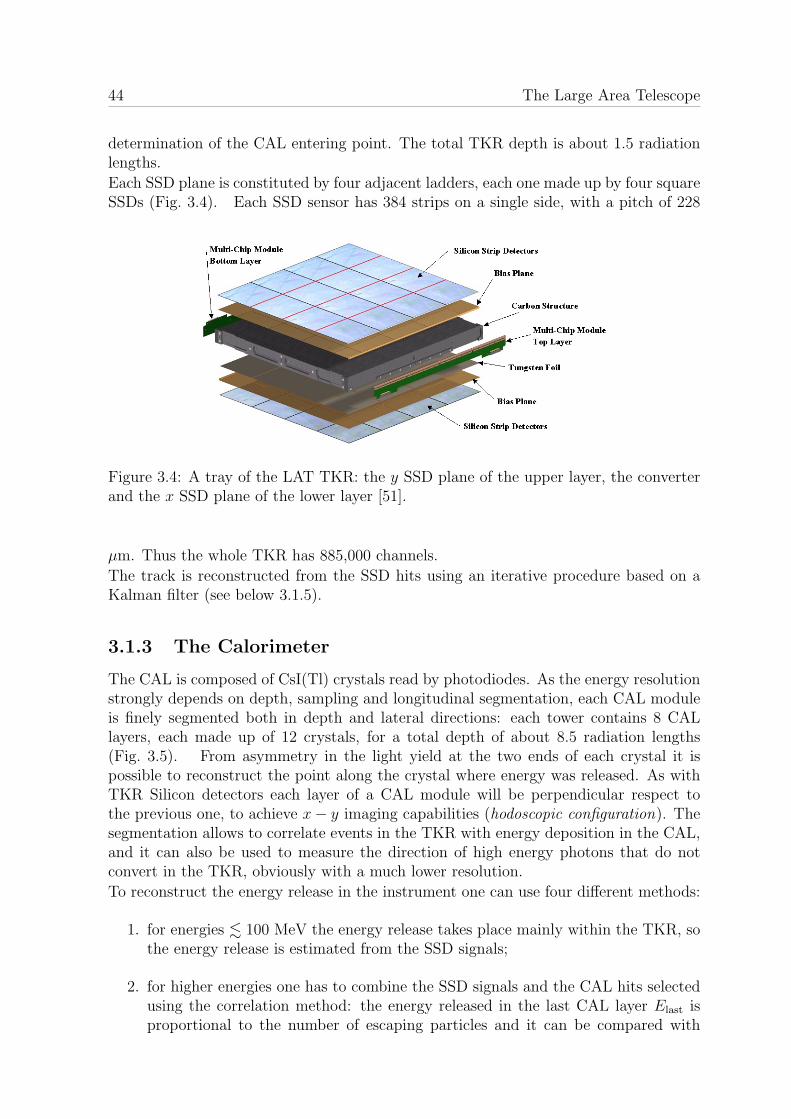
44 The Large Area Telescope
determination of the CAL entering point. The total TKR depth is about 1.5 radiationlengths.
Each SSD plane is constituted by four adjacent ladders, each one made up by four squareSSDs (Fig. 3.4). Each SSD sensor has 384 strips on a single side, with a pitch of 228
Figure 3.4: A tray of the LAT TKR: the y SSD plane of the upper layer, the converterand the x SSD plane of the lower layer [51].
µm. Thus the whole TKR has 885,000 channels.
The track is reconstructed from the SSD hits using an iterative procedure based on aKalman filter (see below 3.1.5).
3.1.3 The Calorimeter
The CAL is composed of CsI(Tl) crystals read by photodiodes. As the energy resolutionstrongly depends on depth, sampling and longitudinal segmentation, each CAL moduleis finely segmented both in depth and lateral directions: each tower contains 8 CALlayers, each made up of 12 crystals, for a total depth of about 8.5 radiation lengths(Fig. 3.5). From asymmetry in the light yield at the two ends of each crystal it ispossible to reconstruct the point along the crystal where energy was released. As withTKR Silicon detectors each layer of a CAL module will be perpendicular respect tothe previous one, to achieve x− y imaging capabilities (hodoscopic configuration). Thesegmentation allows to correlate events in the TKR with energy deposition in the CAL,and it can also be used to measure the direction of high energy photons that do notconvert in the TKR, obviously with a much lower resolution.
To reconstruct the energy release in the instrument one can use four different methods:
1. for energies . 100 MeV the energy release takes place mainly within the TKR, sothe energy release is estimated from the SSD signals;
2. for higher energies one has to combine the SSD signals and the CAL hits selectedusing the correlation method: the energy released in the last CAL layer Elast isproportional to the number of escaping particles and it can be compared with
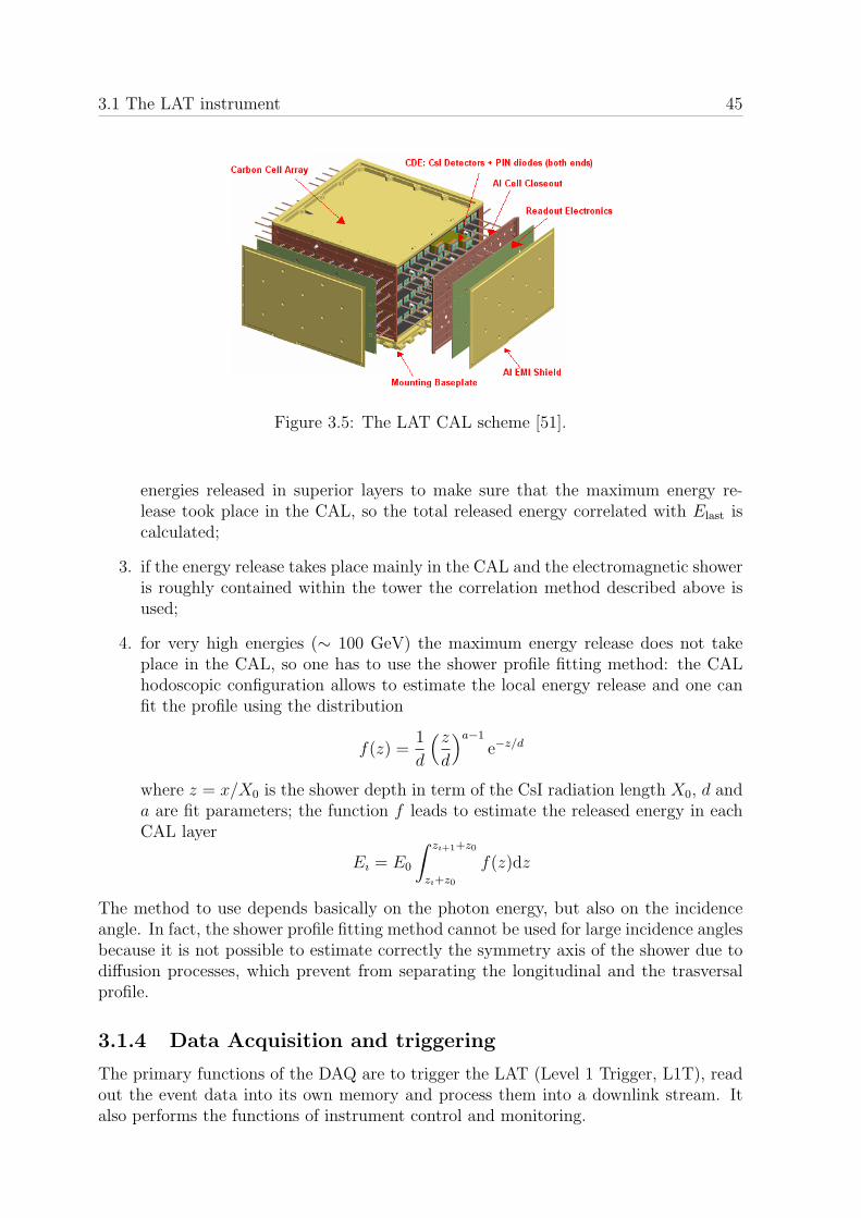
3.1 The LAT instrument 45
Figure 3.5: The LAT CAL scheme [51].
energies released in superior layers to make sure that the maximum energy re-lease took place in the CAL, so the total released energy correlated with Elast iscalculated;
3. if the energy release takes place mainly in the CAL and the electromagnetic showeris roughly contained within the tower the correlation method described above isused;
4. for very high energies (∼ 100 GeV) the maximum energy release does not takeplace in the CAL, so one has to use the shower profile fitting method: the CALhodoscopic configuration allows to estimate the local energy release and one canfit the profile using the distribution
f(z) =1
d
(zd
)a−1
e−z/d
where z = x/X0 is the shower depth in term of the CsI radiation length X0, d anda are fit parameters; the function f leads to estimate the released energy in eachCAL layer
Eı = E0
∫ zı+1+z0
zı+z0
f(z)dz
The method to use depends basically on the photon energy, but also on the incidenceangle. In fact, the shower profile fitting method cannot be used for large incidence anglesbecause it is not possible to estimate correctly the symmetry axis of the shower due todiffusion processes, which prevent from separating the longitudinal and the trasversalprofile.
3.1.4 Data Acquisition and triggering
The primary functions of the DAQ are to trigger the LAT (Level 1 Trigger, L1T), readout the event data into its own memory and process them into a downlink stream. Italso performs the functions of instrument control and monitoring.

46 The Large Area Telescope
The L1T generates primitives, which will be used by the following trigger engines. TheL1T does not take in account the ACD information.The first processing level is the Level 2 Trigger (L2T), which is performed locally at thetower level.The L2T implements the ACD veto, rejecting obvious background eventsefficiently and quickly with loose cuts. It is able to remove about any residual TKRtriggers due to stochastic noise. A fast track finding algorithm is used to extrapolatetrack candidates and intersect them with ACD tiles to search for vetoes. Events witha high-energy CAL signature are not rejected, to avoid self-vetoing. The L2T alsoseparates signals produced by MIPs from those from heavy nuclei. Events passingL2T are transmitted to a processor located in the Spacecraft Interface Unit (SIU) foradditional filtering (L3T, Level 3 Trigger).The L3T gathers data from all towers, reconstructs tracks which pass through differenttowers and rejects Earth albedo γ-rays. Events passing L3T are sent to the SpacecraftSolid State Recorder (SSR) for later downlink (every two orbits).
3.1.5 Track and energy release reconstruction
For each event identified as a photon one wants to estimate the incoming directionand the energy. For photons with energy greater than ∼ 20 MeV the most importantinteraction process is pair production. In the TKR charged particles, e− and e+, looseenergy in the SSDs, leading to estimate their energy, their angle of incidence and theirposition. One can define a state vector vk for the k-th plane
vk =
positiontrack slope
energy
If Hk is the matrix which transforms the state vector into the vector of the measurablequantities mk, and εk is the errors vector
mk = Hkvk + εk
The state vector has a temporal evolution, which one can describe as
vk+1 = Fkvk + wk
where Fk describes the deterministic evolution and wk the stochastic component dueto Coulomb Multiple Scattering. One can assume that εk and wk are independent andthat their average is null.The track reconstruction is based on a two step process (Fig. 3.6):
1. at first we estimate vk from mk−1 in each TKR plane;
2. then the Kalman filter estimates again vk from vk+1 smoothing the track from thebottom to the top.
When a candidate track is identified it is related with a CAL shower, whose energy anddirection is determined according to procedures described in 3.1.3. Then the CAL en-tering point is related with the best candidate track, using an automatic algorithm, and

3.2 The Instrument Response Functions 47
Figure 3.6: The track reconstruction process. On the left first step: the red point is theSSD hit in each plane, the blue point the predicted position in the following plane. Onthe right second step: the blue point is the position estimated in each plane in the firststep, the green point the smoothed position in the previous plane by the Kalman filter.
the track reconstruction process takes place again. Finally the best energy associatedwith the track is estimated.
Note that some instrument analysis procedures described in this section have been re-cently revised: we presented the state of art at the DC2 closeout (see 3.2.2), whichcorresponds to the standard used in this work.
3.2 The Instrument Response Functions
3.2.1 IRF definition
In high energy astrophysics it is conventional to use for data analysis a high-level modelof the instrument response through Instrument Response Functions (IRFs). This choiceis motivated by two different purposes:
• instrument analysis is not easily manageable by the external scientific community,so data are released in form of photons tables, which contains just a few estimatedquantities like energy, direction, inclination angle respect to the telescope . . . ;
• IRFs are useful to put together and compare data from different instruments indifferent energy ranges, to perform a multiwavelength analysis.
The instrument response connects the true photon energy E ′ and direction p′ with themeasured quantities E and p. It is conventional to factorize the instrument response
48 The Large Area Telescope
into three functions, plus a temporal scaling factor:
R(E, p|E ′, p′; t) = T (t)A(E ′, p′)D(E|E ′, p′)P (p|E ′, p′) (3.1)
The scaling factor T (t) accounts for temporal effects, such as instrument failures, tem-porary switching off, thermal expansion, . . . . We assume that temporal variations whichcannot be expressed as a scaling factor are negligible over a time interval long enough.The three functions known as IRFs are:
• the effective area A(E ′, p′), which is the efficiency multiplied for the geometricalarea of the detector A0
A = A0 ·Ndetected
Nincident
• the energy dispersion D(E|E ′, p′), i.e. the probability density that a photon withenergy E ′ and direction p′ is detected with energy E
• the Point Spread Function (PSF) P (p|E ′, p′), i.e. the probability density that aphoton with energy E ′ and direction p′ is detected with direction p.
If S(E ′, p′, t) is the source model (i.e. the differential flux dΦ/dE ′ of our model) theexpected observed distribution of count hits is
M(E, p, t) =
∫dE ′dp′R(E, p|E ′, p′; t)S(E ′, p′, t) (3.2)
3.2.2 IRF development: the simulation tools
GLEAM
IRFs are evaluated using Montecarlo simulations. The main simulation package isGLEAM, GLAST LAT Event Analysis Machine, based on the Geant4 (G4) toolkit.Geant4 is integrated into a general framework used to process events, providing a de-tailed simulation of the electronic signals inside Silicon detectors and an accurate de-scription of the instrument. The Gaudi C++ framework manages the loop of particles tobe simulated: then the output from the simulation is stored in the same format as forreal data.The Source Generation is the first algorithm called within the particle loop. This algo-rithm stores the information about the temporal and spectral behavior of the source, aswell as the orbital characteristics of GLAST and additional incoming particles. Withinthis package a series of default sources are implemented. An extension of this frameworkhas been implemented for simulating transient sources such as GRBs.The interactions between particles and detector are simulated using G4. The Run Man-ager proceeds through the following steps:
DetectorConstruction which provides the list of the materials and the geometry ofthe detector, stored in an XML repository;
PhysicsList which describes the interaction processes;
PrimaryGeneratorAction which accounts for production and injection of primaryparticles in the detector;

3.2 The Instrument Response Functions 49
DetectorManager which manages the setup and working of the sensitive detectors.
A detailed description of the signals in the subsystems is provided by a dedicated dig-itization package. Then the same Reconstruction Package as for real data processessignals.
To validate the Montecarlo simulations a beam test was carried out at CERN in 2006.A Calibration Unit (CU), composed by two TKR modules and three CAL elements, wasused to better understand the behavior of different particles as they strike the detectorat different angles. Results are also being used to tune aspects of the reconstructionprocess. Beam testing was conducted at low energies at the Proton Synchrotron (PS)(using electrons with a momentum of 1-5 GeV, positrons of 1 GeV, protons of 6-10 GeV,gammas, both tagged and non tagged, of 0.5-2.5 GeV), and at high energies at the SuperProton Synchrotron (SPS) (using electrons with a momentum of 10-300 GeV, protonsof 20-100 GeV, pions of 20 GeV) and for heavy nuclei at the GSI (using C nuclei with amomentum of 1.5 GeV and Xe of 1 GeV), to ensure Montecarlo simulations of GLEAMadheres as much as possible to the real behavior of the detector.
Unfortunately none of the beam test results was included in analysis at the time of theDC2 closeout.
IRF modeling
After fixing all analysis cuts, defining background rejection, PSF and energy dispersion(and therefore efficiency, energy resolution and angular resolution) one can use simulateddata to model IRFs. IRFs are calculated in form of matrices containing IRFs parametersin different energy logarithmic bins and cosine of inclination angle bins.
Several simulations were performed by the LAT collaboration. Each change in simulationand analysis in principle would warrant an IRF set, but official IRF sets are releasedperiodically after dedicated simulations.
Data Challenges are simulations based on a “realistic” sky-model: they are useful tomodel IRFs, but also to investigate LAT scientific opportunities and to test the analysissoftware in preparation. The one we consider in this work was the Data Challenge 2(DC2), ultimated in May 2006, which simulated 55 days of observations using a sky-model including variable sources like AGNs and pulsars, with the first detailed simulationof the charged background. To model IRFs dedicated simulations utilize a very intensesource isotropic in cosine of inclination angle and uniform in energy decades (dN/dE ∝E−1).
3.2.3 DC2 IRFs
In this paragraph we will present the DC2 IRFs, which will be used in the followingchapters. One can classify filtered events in classes, depending on the probability thatthe event is good (a real photon with adequate energy and angular resolutions). For DC2events were classified in two classes: class A, which satisfies GLAST Science requirementsexcept for effective area (Table 1.1), and class B, which maximize effective area with areasonable PSF and energy dispersion. All events were also divided in front and backconverting (the conversion took place in the thin or in the thick converters).
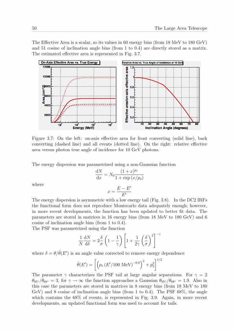
50 The Large Area Telescope
The Effective Area is a scalar, so its values in 60 energy bins (from 18 MeV to 180 GeV)and 51 cosine of inclination angle bins (from 1 to 0.4) are directly stored as a matrix.The estimated effective area is represented in Fig. 3.7.
Figure 3.7: On the left: on-axis effective area for front converting (solid line), backconverting (dashed line) and all events (dotted line). On the right: relative effectivearea versus photon true angle of incidence for 10 GeV photons.
The energy dispersion was parametrized using a non-Gaussian function
dN
dx= N0
(1 + x)p1
1 + exp (x/p2)
where
x =E − E ′
E ′
The energy dispersion is asymmetric with a low energy tail (Fig. 3.8). In the DC2 IRFsthe functional form does not reproduce Montecarlo data adequately enough; however,in more recent developments, the function has been updated to better fit data. Theparameters are stored in matrices in 16 energy bins (from 18 MeV to 180 GeV) and 6cosine of inclination angle bins (from 1 to 0.4).The PSF was parametrized using the function
1
N
dN
dδ= 2
δ
σ
(1− 1
γ
) [1 +
1
2γ
(δ
σ
)2]−γ
where δ = θ/θ(E ′) is an angle value corrected to remove energy dependence
θ(E ′) =
[(p1 (E ′/100 MeV)
−0.8)2
+ p22
]1/2
The parameter γ characterizes the PSF tail at large angular separations. For γ = 2θ95/θ68 = 3, for γ → ∞ the function approaches a Gaussian θ95/θ68 = 1.9. Also inthis case the parameters are stored in matrices in 8 energy bins (from 18 MeV to 180GeV) and 8 cosine of inclination angle bins (from 1 to 0.4). The PSF 68%, the anglewhich contains the 68% of events, is represented in Fig. 3.9. Again, in more recentdevelopments, an updated functional form was used to account for tails.
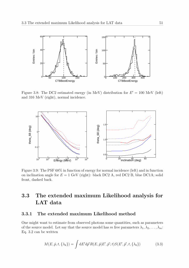
3.3 The extended maximum Likelihood analysis for LAT data 51
CTBBestEnergy
Ent
ries
/ bin
50 100 1500
20
40
60
CTBBestEnergy
Ent
ries
/ bin
0 100 200 300 4000
50
100
150
E0 = 1000, inc = 0 E0 = 3162, inc = 0
Figure 3.8: The DC2 estimated energy (in MeV) distribution for E ′ = 100 MeV (left)and 316 MeV (right), normal incidence.
Energy (MeV)
thet
a_68
(de
g)
101
102
103
104
105
106
0.1
1
10
normal incidence
inclination (deg)
thet
a_68
(de
g)
0 20 40 60
0.5
1.0
1.5
Figure 3.9: The PSF 68% in function of energy for normal incidence (left) and in functionon inclination angle for E = 1 GeV (right): black DC2 A, red DC2 B, blue DC1A; solidfront, dashed back.
3.3 The extended maximum Likelihood analysis for
LAT data
3.3.1 The extended maximum Likelihood method
One might want to estimate from observed photons some quantities, such as parametersof the source model. Let say that the source model has m free parameters λ1, λ2, . . . , λm:Eq. 3.2 can be written
M(E, p, t, λk) =
∫dE ′dp′R(E, p|E ′, p′; t)S(E ′, p′, t, λk) (3.3)
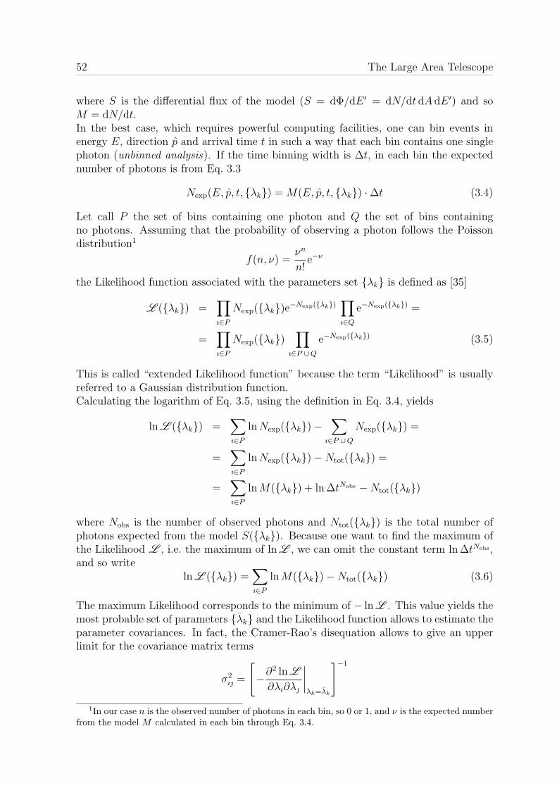
52 The Large Area Telescope
where S is the differential flux of the model (S = dΦ/dE ′ = dN/dt dA dE ′) and soM = dN/dt.In the best case, which requires powerful computing facilities, one can bin events inenergy E, direction p and arrival time t in such a way that each bin contains one singlephoton (unbinned analysis). If the time binning width is ∆t, in each bin the expectednumber of photons is from Eq. 3.3
Nexp(E, p, t, λk) = M(E, p, t, λk) ·∆t (3.4)
Let call P the set of bins containing one photon and Q the set of bins containingno photons. Assuming that the probability of observing a photon follows the Poissondistribution1
f(n, ν) =νn
n!e−ν
the Likelihood function associated with the parameters set λk is defined as [35]
L (λk) =∏ı∈P
Nexp(λk)e−Nexp(λk)∏ı∈Q
e−Nexp(λk) =
=∏ı∈P
Nexp(λk)∏
ı∈P ∪Q
e−Nexp(λk) (3.5)
This is called “extended Likelihood function” because the term “Likelihood” is usuallyreferred to a Gaussian distribution function.Calculating the logarithm of Eq. 3.5, using the definition in Eq. 3.4, yields
ln L (λk) =∑ı∈P
lnNexp(λk)−∑
ı∈P ∪Q
Nexp(λk) =
=∑ı∈P
lnNexp(λk)−Ntot(λk) =
=∑ı∈P
lnM(λk) + ln ∆tNobs −Ntot(λk)
where Nobs is the number of observed photons and Ntot(λk) is the total number ofphotons expected from the model S(λk). Because one want to find the maximum ofthe Likelihood L , i.e. the maximum of ln L , we can omit the constant term ln ∆tNobs ,and so write
ln L (λk) =∑ı∈P
lnM(λk)−Ntot(λk) (3.6)
The maximum Likelihood corresponds to the minimum of − ln L . This value yields themost probable set of parameters λk and the Likelihood function allows to estimate theparameter covariances. In fact, the Cramer-Rao’s disequation allows to give an upperlimit for the covariance matrix terms
σ2ı =
[−∂
2 ln L
∂λı∂λ
∣∣∣∣λk=λk
]−1
1In our case n is the observed number of photons in each bin, so 0 or 1, and ν is the expected numberfrom the model M calculated in each bin through Eq. 3.4.
3.3 The extended maximum Likelihood analysis for LAT data 53
The maximum Likelihood method allows also to compare different models. The mostpowerful criterion is the Likelihood ratio test. According to Wilk’s theorem, if weconsider a model M with m parameters and a second model M0 with a subset of h < mparameters the test statistic
TS = 2 (ln L − ln L0)
is distributed asymptotically as a χ2 with k = m− h degrees of freedom.
3.3.2 The unbinned analysis
The Likelihood method described above in 3.3.1 is used in the unbinned analysis pro-cedure for LAT data. Detailed information about LAT software is given in the UserWorkbook [4]. In this paragraph we summarize the main steps in the analysis proce-dure:
1. selecting events in a Region Of Interest (ROI);
2. calculating lifetimes in function of energy and cosine of inclination angle (ex-pCube);
3. developing a source model S(λk), which has to account for emission in a regionwider than the ROI to avoid systematics effects;
4. separately calculating the instrument exposure is required to avoid excessive timelosses, especially in the analysis of extended sources: the exposure E is defined as
E =
∫dt dE ′ dp′ T (t)A(E ′, p′)
in several time bins, logarithmic energy bins and cosine of incidence angle bins2;in each bin one can obtain the expected number of photons multiplying the modelflux for the corresponding exposure
Nexp = EdΦ
dE
5. fit the model parameters λk against the observed counts; as described in 3.3.1,first one convolves the source model S with the IRFs to obtain the expected distri-bution of observed photons M (Eq. 3.3), then calculates the Likelihood logarithm(Eq. 3.6) and maximize it to find the most probable set of parameters λk withtheir covariance matrix.
2The grid used for the exposure calculation is much wider than the one used to calculate theLikelihood.

54 The Large Area Telescope
3.3.3 The binned analysis
One might want to analyze data in a big region of the sky, not being particularlyinterested in reaching a very high precision in source location. This is the case ofextended sources, such as the diffuse emission presented in chapter 2. To avoid excessivecomputing times it might be suitable to use a binned Likelihood analysis, which is lessaccurate but absolutely faster than unbinned analysis presented in the previous 3.3.2.The main steps for a binned analysis are:
1. making a counts map binning data according to their direction and energy3;
2. as for the unbinned analysis, calculating lifetimes in function of energy and cosineof inclination angle (expCube);
3. as for the unbinned analysis, developing a source model S(λk);
4. calculating a binned exposure, which is the exposure
E =
∫dt dE ′ dp′ T (t)A(E ′, p′)
binned using the same intervals in space and energy as in the counts map;
5. making a source map, i.e. a map of the predicted counts in each bin convolvingthe source model with IRFs;
6. calculating the Likelihood L (λk) (the formula is different from that in Eq. 3.5,following the generic definition of the Likelihood function4 ) and fit the modelparameters to obtain the most probable values λk and their covariances.
3Energy bins are usually logarithmic because the spectrum is expected to have a power law likebehavior, according to the idea that the most common acceleration mechanism which leads to γ-rayproduction is the Fermi mechanism, see appendix A.
4In general, if one has a stochastic variable x distributed following a density probability f(x, λk)and a sample of observations x1, x2, . . . , xN , the Likelihood function associated with the set of param-eters λk is
L (λk) =N∏
ı=1
f(xı, λk)
55
Chapter 4
A model for analysis of gamma-rayemission from molecular clouds
This chapter is devoted to the development of an analysis model for γ-ray emissionfrom molecular clouds suitable for LAT data analysis and to its tests on simulated data.At first we simulated only the galactic diffuse emission, whereas in a second time, inthe next chapter, we will analyze a more realistic data sample, including the EGRB andpoint sources. In section 1 we present the GALPROP model our Montecarlo simulationsare based on and we describe the procedure adopted for LAT observation simulation. Insection 2 we investigate the effects of some approximations in our analysis model (thelocal power law spectrum and the isotropy for IC emission) and we try to understandif the uncertainties on the spectrum affect the determination of the emissivities, whichallow to trace the local CR abundance and to calibrate the X-ratio. In section 3 weapply our analysis model to reconstruct the emission spectrum of molecular clouds, and,in section 4, we compare our results with the original GALPROP model, giving a roughestimate of systematic errors involved.
4.1 The simulation
To develop an analysis model for the diffuse emission from molecular clouds suitablefor LAT data, we practiced using simulated data. We decided to analyze simulateddata in Monoceros, a region well known from EGRET data [22]. In this region thereare molecular clouds located in the outer Galaxy, leading theoretically to calibrate theX-ratio beyond the Solar circle.
4.1.1 The GALPROP model
The GALPROP model used in this work is based on the model 49 6002029RE, developedfor Milagro data analysis of the diffuse emission in Cygnus region [5], already introducedin 2.2.3. It is an optimized model tuned to describe diffuse γ-rays up to 100 TeV with ahalo radius of 20 kpc and height of 4 kpc. It uses a cylindrical symmetry in CR sourcedistribution and in solution of the transport equation.We modified this model to obtain γ-ray skymaps using GALPROP 50p. We used the upto date ISRF model by Porter [44] described in 2.2.1, and up to date isotopic abundances
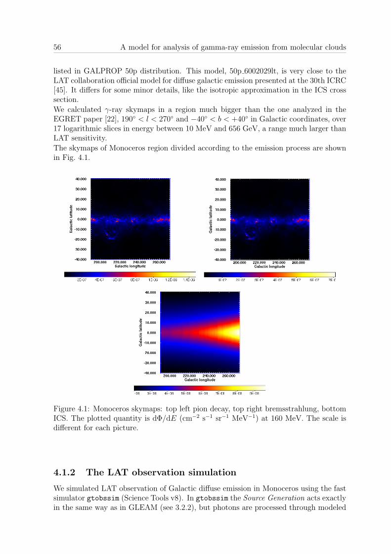
56 A model for analysis of gamma-ray emission from molecular clouds
listed in GALPROP 50p distribution. This model, 50p 6002029lt, is very close to theLAT collaboration official model for diffuse galactic emission presented at the 30th ICRC[45]. It differs for some minor details, like the isotropic approximation in the ICS crosssection.
We calculated γ-ray skymaps in a region much bigger than the one analyzed in theEGRET paper [22], 190 < l < 270 and −40 < b < +40 in Galactic coordinates, over17 logarithmic slices in energy between 10 MeV and 656 GeV, a range much larger thanLAT sensitivity.
The skymaps of Monoceros region divided according to the emission process are shownin Fig. 4.1.
Figure 4.1: Monoceros skymaps: top left pion decay, top right bremsstrahlung, bottomICS. The plotted quantity is dΦ/dE (cm−2 s−1 sr−1 MeV−1) at 160 MeV. The scale isdifferent for each picture.
4.1.2 The LAT observation simulation
We simulated LAT observation of Galactic diffuse emission in Monoceros using the fastsimulator gtobssim (Science Tools v8). In gtobssim the Source Generation acts exactlyin the same way as in GLEAM (see 3.2.2), but photons are processed through modeled

4.2 Tests at high energies 57
IRFs, and only tables containing a few estimated quantities (like energy, direction, . . . )are produced in output.The main simulation characteristics are:
• a whole year of LAT observation in survey mode1;
• acceptance cone of 35 centered on l = 230, b = 0;
• we used DC2 IRFs, all events class A+B (see 3.2.3);
Counts maps of our simulation are shown in Fig. 4.2.
Figure 4.2: Counts map of LAT observation simulation over the whole energy range 30MeV-200 GeV: left pion decay, center bremsstrahlung, right ICS. Cartesian projectioncentered on l = 230, b = 0 with an acceptance cone of 35.
4.2 Tests at high energies
We started analyzing data at high energies, between 1 GeV and 30 GeV, for two reasons:
• the spectral behavior at high energies is much simpler, close to a power law;
• the instrument performances are better: in particular the good PSF allows todiscriminate contributions from gas in different galactocentric annuli thanks totheir different spatial distribution.
We assume, as it was done in EGRET analysis (see 2.3.1), that the photon flux is locallyproportional to the gas column density in four galactocentric rings, which we describeusing the same naming scheme as in EGRET analysis2:
1The survey mode will be the standard observation mode in the first two years: the LAT will scanthe whole sky every two orbits rocking, i.e. moving up and down of 35 with respect to the telescopezenith.
2In our analysis these are just figurative names, because GALPROP does not take into accountstructures like Galaxy arms in CR propagation. It of course does for generation of γ-ray skymaps andradius ranges in analysis are the same as used by GALPROP (see 2.2.1).
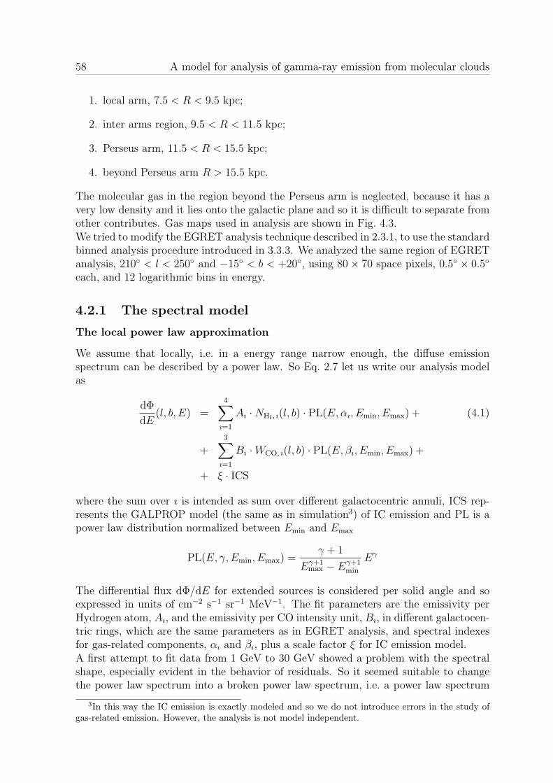
58 A model for analysis of gamma-ray emission from molecular clouds
1. local arm, 7.5 < R < 9.5 kpc;
2. inter arms region, 9.5 < R < 11.5 kpc;
3. Perseus arm, 11.5 < R < 15.5 kpc;
4. beyond Perseus arm R > 15.5 kpc.
The molecular gas in the region beyond the Perseus arm is neglected, because it has avery low density and it lies onto the galactic plane and so it is difficult to separate fromother contributes. Gas maps used in analysis are shown in Fig. 4.3.We tried to modify the EGRET analysis technique described in 2.3.1, to use the standardbinned analysis procedure introduced in 3.3.3. We analyzed the same region of EGRETanalysis, 210 < l < 250 and −15 < b < +20, using 80× 70 space pixels, 0.5 × 0.5
each, and 12 logarithmic bins in energy.
4.2.1 The spectral model
The local power law approximation
We assume that locally, i.e. in a energy range narrow enough, the diffuse emissionspectrum can be described by a power law. So Eq. 2.7 let us write our analysis modelas
dΦ
dE(l, b, E) =
4∑ı=1
Aı ·NHI, ı(l, b) · PL(E,αı, Emin, Emax) + (4.1)
+3∑
ı=1
Bı ·WCO, ı(l, b) · PL(E, βı, Emin, Emax) +
+ ξ · ICS
where the sum over ı is intended as sum over different galactocentric annuli, ICS rep-resents the GALPROP model (the same as in simulation3) of IC emission and PL is apower law distribution normalized between Emin and Emax
PL(E, γ, Emin, Emax) =γ + 1
Eγ+1max − Eγ+1
min
Eγ
The differential flux dΦ/dE for extended sources is considered per solid angle and soexpressed in units of cm−2 s−1 sr−1 MeV−1. The fit parameters are the emissivity perHydrogen atom, Aı, and the emissivity per CO intensity unit, Bı, in different galactocen-tric rings, which are the same parameters as in EGRET analysis, and spectral indexesfor gas-related components, αı and βı, plus a scale factor ξ for IC emission model.A first attempt to fit data from 1 GeV to 30 GeV showed a problem with the spectralshape, especially evident in the behavior of residuals. So it seemed suitable to changethe power law spectrum into a broken power law spectrum, i.e. a power law spectrum
3In this way the IC emission is exactly modeled and so we do not introduce errors in the study ofgas-related emission. However, the analysis is not model independent.
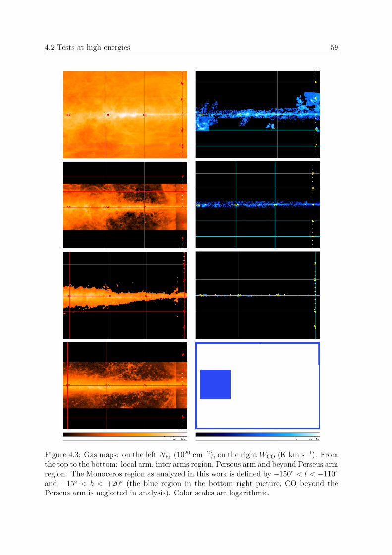
4.2 Tests at high energies 59
Figure 4.3: Gas maps: on the left NHI(1020 cm−2), on the right WCO (K km s−1). From
the top to the bottom: local arm, inter arms region, Perseus arm and beyond Perseus armregion. The Monoceros region as analyzed in this work is defined by −150 < l < −110
and −15 < b < +20 (the blue region in the bottom right picture, CO beyond thePerseus arm is neglected in analysis). Color scales are logarithmic.
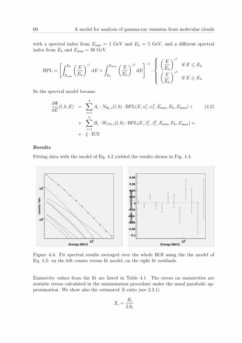
60 A model for analysis of gamma-ray emission from molecular clouds
with a spectral index from Emin = 1 GeV and Eb = 5 GeV, and a different spectralindex from Eb and Emax = 30 GeV
BPL =
[∫ Eb
Emin
(E
Eb
)γ1
dE +
∫ Emax
Eb
(E
Eb
)γ2
dE
]−1
·
(E
Eb
)γ1
if E ≤ Eb(E
Eb
)γ2
if E ≥ Eb
So the spectral model became
dΦ
dE(l, b, E) =
4∑ı=1
Aı ·NHI, ı(l, b) · BPL(E,α1ı , α
2ı , Emin, Eb, Emax) + (4.2)
+3∑
ı=1
Bı ·WCO, ı(l, b) · BPL(E, β1ı , β
2ı , Emin, Eb, Emax) +
+ ξ · ICS
Results
Fitting data with the model of Eq. 4.2 yielded the results shown in Fig. 4.4.
Energy (MeV)
410
cou
nts
/ b
in
310
410
Energy (MeV)
410
(co
un
ts -
mo
del
)/m
od
el
-0.1
-0.08
-0.06
-0.04
-0.02
0
0.02
0.04
0.06
0.08
Figure 4.4: Fit spectral results averaged over the whole ROI using the the model ofEq. 4.2: on the left counts versus fit model, on the right fit residuals.
Emissivity values from the fit are listed in Table 4.1. The errors on emissivities arestatistic errors calculated in the minimization procedure under the usual parabolic ap-proximation. We show also the estimated X-ratio (see 2.3.1)
Xı =Bı
2Aı
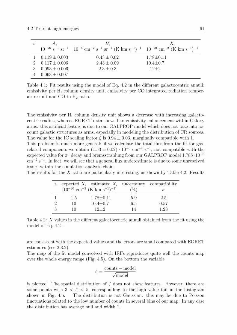
4.2 Tests at high energies 61
ı Aı Bı Xı
10−26 s−1 sr−1 10−6 cm−2 s−1 sr−1 (K km s−1)−1 10−20 cm−2 (K km s−1)−1
1 0.119± 0.003 0.43± 0.02 1.78±0.112 0.117± 0.006 2.43± 0.09 10.4±0.73 0.093± 0.006 2.3± 0.3 12±24 0.063± 0.007
Table 4.1: Fit results using the model of Eq. 4.2 in the different galactocentric annuli:emissivity per HI column density unit, emissivity per CO integrated radiation temper-ature unit and CO-to-H2 ratio.
The emissivity per HI column density unit shows a decrease with increasing galacto-centric radius, whereas EGRET data showed an emissivity enhancement within Galaxyarms: this artificial feature is due to our GALPROP model which does not take into ac-count galactic structures as arms, especially in modeling the distribution of CR sources.The value for the IC scaling factor ξ is 0.94± 0.03, marginally compatible with 1.This problem is much more general: if we calculate the total flux from the fit for gas-related components we obtain (1.53 ± 0.02) · 10−6 cm−2 s−1, not compatible with theexpected value for π0 decay and bremsstrahlung from our GALPROP model 1.785 ·10−6
cm−2 s−1. In fact, we will see that a general flux underestimate is due to some unresolvedissues within the simulation-analysis chain.The results for the X-ratio are particularly interesting, as shown by Table 4.2. Results
ı expected Xı estimated Xı uncertainty compatibility[10−20 cm−2 (K km s−1)−1] (%) σ
1 1.5 1.78±0.11 5.9 2.52 10 10.4±0.7 6.5 0.573 10 12±2 14 1.28
Table 4.2: X values in the different galactocentric annuli obtained from the fit using themodel of Eq. 4.2 .
are consistent with the expected values and the errors are small compared with EGRETestimates (see 2.3.2).The map of the fit model convolved with IRFs reproduces quite well the counts mapover the whole energy range (Fig. 4.5). On the bottom the variable
ζ =counts−model√
model
is plotted. The spatial distribution of ζ does not show features. However, there aresome points with 3 < ζ < 5, corresponding to the high value tail in the histogramshown in Fig. 4.6. The distribution is not Gaussian: this may be due to Poissonfluctuations related to the low number of counts in several bins of our map. In any casethe distribution has average null and width 1.

62 A model for analysis of gamma-ray emission from molecular clouds
Figure 4.5: On the top counts map (left) versus model map after the fit using the modelof Eq. 4.2 (right) over the whole energy range. On the bottom the ζ map.
h1Entries 5600Mean 0.0138± 0.0003929 RMS 0.009758± 1.033
/ ndf 2χ 180.4 / 34Constant 7.4± 445.2 Mean 0.0149± -0.0062 Sigma 0.0095± 0.9718
ζ-6 -4 -2 0 2 4 6
0
50
100
150
200
250
300
350
400
450
h1Entries 5600Mean 0.0138± 0.0003929 RMS 0.009758± 1.033
/ ndf 2χ 180.4 / 34Constant 7.4± 445.2 Mean 0.0149± -0.0062 Sigma 0.0095± 0.9718
histogramζ
Figure 4.6: Histogram of ζ values from the fit using the model in Eq. 4.2.

4.2 Tests at high energies 63
4.2.2 The spatial distribution of IC emission
The isotropic model
In EGRET analysis the IC emission was modeled using an isotropic term (see 2.3.1),but GALPROP models led to think that IC emission plays a more important role thanwhat was thought before [38]. So we want to understand if the isotropic approximationfor ICS can be used for LAT data analysis, considered the better PSF with respectto EGRET. We modeled IC emission using an isotropic term with a local power lawspectrum, so our fit model became
dΦ
dE(l, b, E) =
4∑ı=1
Aı ·NHI, ı(l, b) · BPL(E,α1ı , α
2ı , Emin, Eb, Emax) + (4.3)
+3∑
ı=1
Bı ·WCO, ı(l, b) · BPL(E, β1ı , β
2ı , Emin, Eb, Emax) +
+ C · BPL(E, γ1ı , γ
2ı , Emin, Eb, Emax)
Fit results
Fitting data with the model of Eq. 4.3 yielded the results shown in Fig. 4.7.
Energy (MeV)
410
cou
nts
/ b
in
310
410
Energy (MeV)
410
(co
un
ts -
mo
del
)/m
od
el
-0.1
-0.05
0
0.05
0.1
Figure 4.7: Fit spectral results averaged over the whole ROI using the the spectralmodel of Eq. 4.3: on the left counts versus fit model, on the right fit residuals.
Emissivity values from the fit are listed in Table 4.3. Results are all compatible withthe previous determination in Table 4.1. Also in this case we have a flux underestimate:the total estimated flux is (1.999 ± 0.008) · 10−6 cm−2 s−1 respect to a value from ourGALPROP model of 2.285 ·10−6 cm−2 s−1. The X-ratio estimate is still good, as shownby Table 4.4The isotropic approximation for the IC emission does not seem to introduce a significantbias: the model map well reproduces the counts map and also the distribution of residual
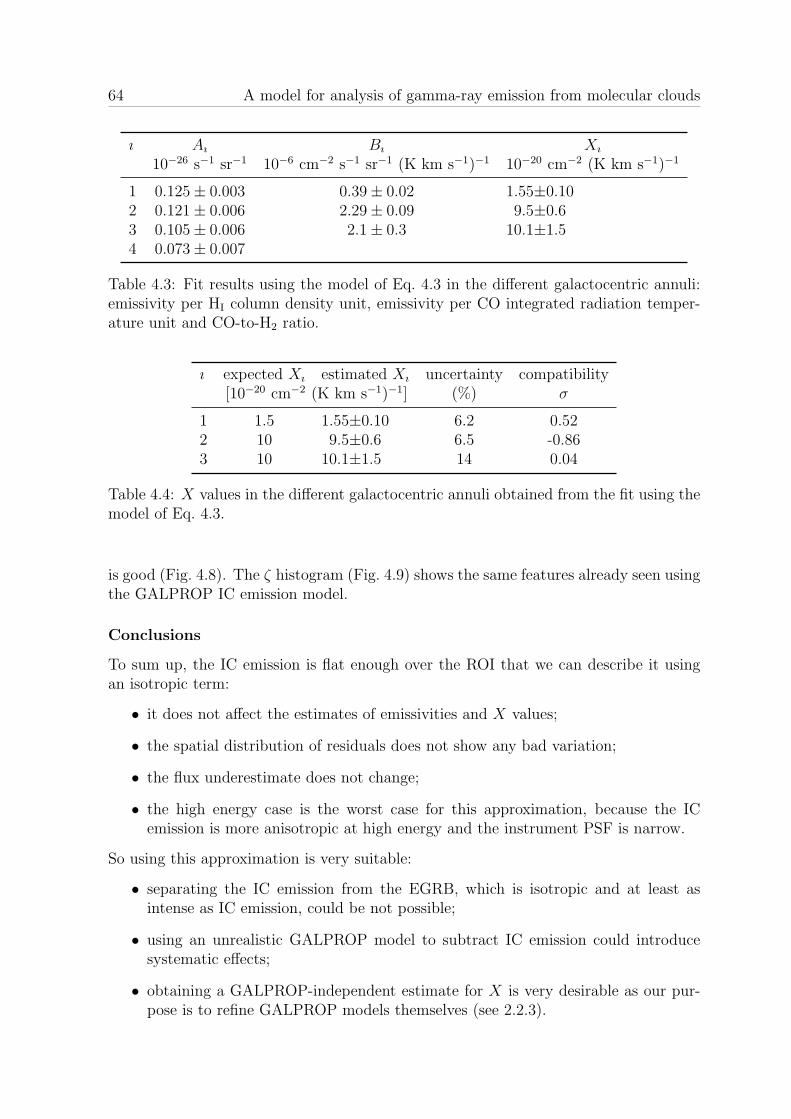
64 A model for analysis of gamma-ray emission from molecular clouds
ı Aı Bı Xı
10−26 s−1 sr−1 10−6 cm−2 s−1 sr−1 (K km s−1)−1 10−20 cm−2 (K km s−1)−1
1 0.125± 0.003 0.39± 0.02 1.55±0.102 0.121± 0.006 2.29± 0.09 9.5±0.63 0.105± 0.006 2.1± 0.3 10.1±1.54 0.073± 0.007
Table 4.3: Fit results using the model of Eq. 4.3 in the different galactocentric annuli:emissivity per HI column density unit, emissivity per CO integrated radiation temper-ature unit and CO-to-H2 ratio.
ı expected Xı estimated Xı uncertainty compatibility[10−20 cm−2 (K km s−1)−1] (%) σ
1 1.5 1.55±0.10 6.2 0.522 10 9.5±0.6 6.5 -0.863 10 10.1±1.5 14 0.04
Table 4.4: X values in the different galactocentric annuli obtained from the fit using themodel of Eq. 4.3.
is good (Fig. 4.8). The ζ histogram (Fig. 4.9) shows the same features already seen usingthe GALPROP IC emission model.
Conclusions
To sum up, the IC emission is flat enough over the ROI that we can describe it usingan isotropic term:
• it does not affect the estimates of emissivities and X values;
• the spatial distribution of residuals does not show any bad variation;
• the flux underestimate does not change;
• the high energy case is the worst case for this approximation, because the ICemission is more anisotropic at high energy and the instrument PSF is narrow.
So using this approximation is very suitable:
• separating the IC emission from the EGRB, which is isotropic and at least asintense as IC emission, could be not possible;
• using an unrealistic GALPROP model to subtract IC emission could introducesystematic effects;
• obtaining a GALPROP-independent estimate for X is very desirable as our pur-pose is to refine GALPROP models themselves (see 2.2.3).
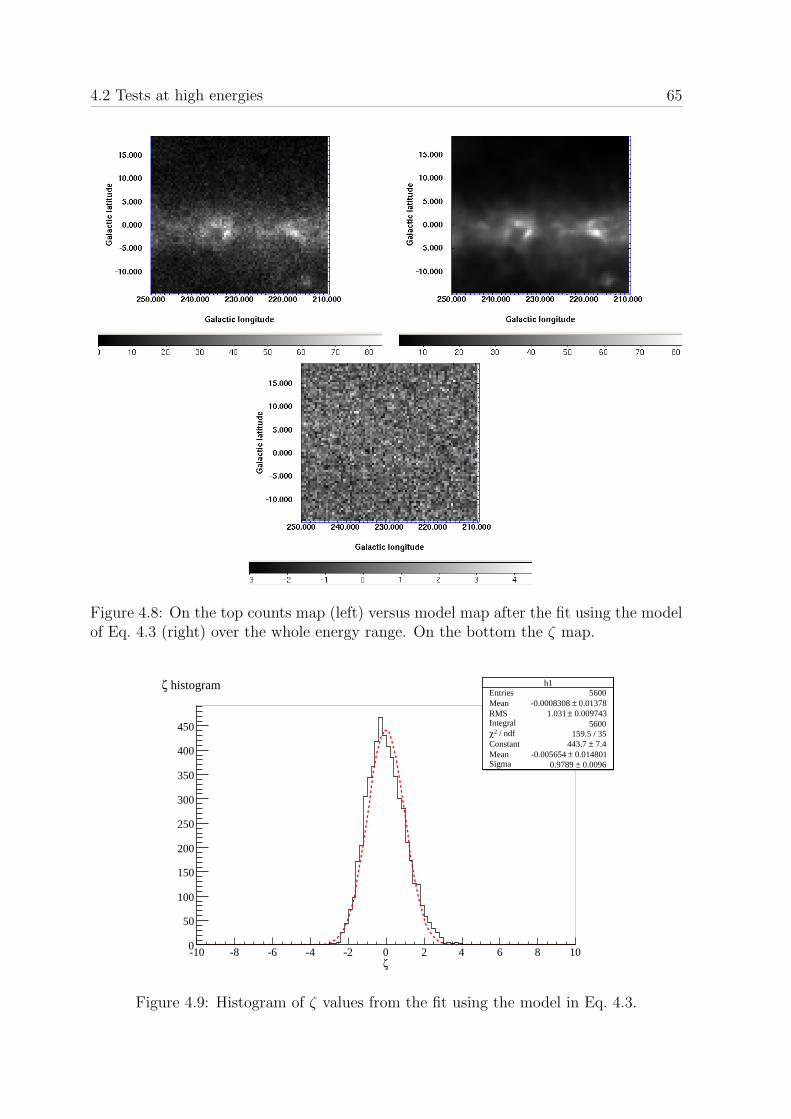
4.2 Tests at high energies 65
Figure 4.8: On the top counts map (left) versus model map after the fit using the modelof Eq. 4.3 (right) over the whole energy range. On the bottom the ζ map.
h1Entries 5600Mean 0.01378± -0.0008308 RMS 0.009743± 1.031 Integral 5600
/ ndf 2χ 159.5 / 35Constant 7.4± 443.7 Mean 0.014801± -0.005654 Sigma 0.0096± 0.9789
ζ-10 -8 -6 -4 -2 0 2 4 6 8 100
50
100
150
200
250
300
350
400
450
h1Entries 5600Mean 0.01378± -0.0008308 RMS 0.009743± 1.031 Integral 5600
/ ndf 2χ 159.5 / 35Constant 7.4± 443.7 Mean 0.014801± -0.005654 Sigma 0.0096± 0.9789
histogramζ
Figure 4.9: Histogram of ζ values from the fit using the model in Eq. 4.3.
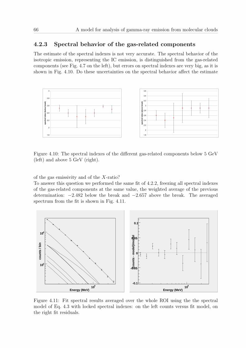
66 A model for analysis of gamma-ray emission from molecular clouds
4.2.3 Spectral behavior of the gas-related components
The estimate of the spectral indexes is not very accurate. The spectral behavior of theisotropic emission, representing the IC emission, is distinguished from the gas-relatedcomponents (see Fig. 4.7 on the left), but errors on spectral indexes are very big, as it isshown in Fig. 4.10. Do these uncertainties on the spectral behavior affect the estimate
1,8
2
2,2
2,4
2,6
2,8
3
spec
tral
inde
x (b
elow
bre
ak)
1,8
2
2,2
2,4
2,6
2,8
3
3,2
3,4
3,6
spec
tral
inde
x (a
bove
bre
ak)
Figure 4.10: The spectral indexes of the different gas-related components below 5 GeV(left) and above 5 GeV (right).
of the gas emissivity and of the X-ratio?To answer this question we performed the same fit of 4.2.2, freezing all spectral indexesof the gas-related components at the same value, the weighted average of the previousdetermination: −2.482 below the break and −2.657 above the break. The averagedspectrum from the fit is shown in Fig. 4.11.
Energy (MeV)
410
cou
nts
/ b
in
310
410
Energy (MeV)
410
(co
un
ts -
mo
del
)/m
od
el
-0.1
-0.05
0
0.05
0.1
Figure 4.11: Fit spectral results averaged over the whole ROI using the the spectralmodel of Eq. 4.3 with locked spectral indexes: on the left counts versus fit model, onthe right fit residuals.

4.3 Extension at low energies 67
The emissivities and the X values are not significantly altered by this position, as shownin Table 4.5 and Table 4.6.
ı Aı Bı Xı
10−26 s−1 sr−1 10−6 cm−2 s−1 sr−1 (K km s−1)−1 10−20 cm−2 (K km s−1)−1
1 0.125± 0.003 0.39± 0.02 1.55±0.102 0.121± 0.006 2.29± 0.09 9.5±0.63 0.105± 0.006 2.1± 0.3 10.1±1.54 0.073± 0.007
Table 4.5: Fit results using the model of Eq. 4.3 with frozen spectral indexes in thedifferent galactocentric annuli: emissivity per HI column density unit, emissivity perCO integrated radiation temperature unit and CO-to-H2 ratio.
ı expected Xı estimated Xı uncertainty compatibility[10−20 cm−2 (K km s−1)−1] (%) σ
1 1.5 1.55±0.10 6.2 0.482 10 9.5±0.7 6.5 -0.813 10 10.1±1.5 14 0.08
Table 4.6: X values in the different galactocentric annuli obtained from the fit using themodel of Eq. 4.3 with frozen spectral indexes.
Also the flux estimate is exactly the same as in the previous case, using free spectralindexes. So we can conclude that, although the determination of the spectral indexes isnot very precise, this issue does not affect the estimate of emissivities, and consequentlyof fluxes and X. The spatial distribution of fit residuals is very close to that shown inFig. 4.8 and Fig. 4.9.If we apply to our fit the Likelihood ratio test, described at 3.3.1, we find that
TS = 2 (ln L − ln L0) = 14.3
where the index 0 represents the model with locked spectral indexes. Since TS is dis-tributed as a χ2 with 16 degrees of freedom we cannot statistically distinguish the twomodels. Of course the results obtained without freezing all spectral indexes to a fixedvalue are preferable.
4.3 Extension at low energies
4.3.1 The multi-energy range analysis
Now we want to extend our analysis to a wider energy interval. Since the relevantphenomenon, to trace CRs and calibrate the X-ratio, is the emission related to gas wehave to consider only energies where this process is dominant. Considering

68 A model for analysis of gamma-ray emission from molecular clouds
• the dominance of IC emission at very low (. 100 MeV) and very high energies(& 50 GeV);
• the worse instrument performances at very low energies (E . 100 MeV)
• the low number of photons at high energies (& 10 GeV)
the possible energy range extends between ∼ 100 MeV and ∼ 50 GeV.To perform a Likelihood fit we need to use a spectral model based on a derivable function,but to use as fit parameters emissivities (and so obtain easily the X-ratio value) we alsoneed to use an integrable function. The only suitable function which has such propertiesis the power law4, or the broken power law, used in 4.2. To use a power law (or brokenpower law) spectrum we need to break the possible energy range in some subranges,because the galactic diffuse spectrum is very different from a simple power law, whichcan be used to approximate it just locally.In fact, separating the analysis in different energy ranges is the most common and themost suitable procedure in astrophysics for many reasons:
• it is the only way to perform a multiwavelength analysis over an energy range notcovered by a single instrument;
• also for data coming from the same instrument in different energy ranges measure-ments can be made using different procedures (for LAT for example the procedureused for the energy estimate depends strongly on the photon energy, see 3.5);
• moreover the background physical processes, which lead to photon production,are in general not well understood and so analysis models are phenomenological;separating analysis in different energy ranges and looking for differences is thesimplest way to obtain hints about the physics of the phenomenon.
This aspect of the analysis procedure is strictly connected with the other one presentedin 3.2.1, the use of IRFs to model the instrument performances.In our case the multi-energy range analysis is particularly suitable because it allowsto point out an energy dependence of the X-ratio, which might be connected with anincomplete penetration of CRs in the interior of molecular clouds (see 2.3.1).We decided to use in each energy range a broken power law spectrum, to be able tohave energy ranges wide enough to obtain reasonable errors on counts. To take intoaccount the instrument performances and the detection processes we decided to dividethe possible energy range for our analysis (100 MeV to 50 GeV) following the IRF binning(see 3.2.3). At high energies changes in the instrument behavior are not so dramaticand we have a few photons, so we adopted a binning based on the PSF, but coarser:between 1 GeV and 32 GeV we used a broken power law spectrum, with a spectral breakat 5.6 GeV (very close to the analysis in 4.2). At lower energies the instrument behavioris more complicated, so we adopted the effective area binning, much finer: between 562MeV and 1 GeV we used a broken power low with a spectral break at 750 GeV. Atenergies lower than 562 MeV our analysis technique did not work, i.e. the fits could notconverge.
4Of course other functions with such properties exist, but we need to keep the computing time, tocalculate derivatives and integrals, reasonably low.

4.3 Extension at low energies 69
This problem is due to the worse PSF, which does not allow to separate gas componentsusing their different spatial distribution. This issue could be overcome using a differentset of IRFs: DC2 IRFs are now dated because great improvements in instrument analysishave been achieved since DC2. Moreover dedicated sets of IRFs will be developed fordifferent scientific analysis topics: in particular an IRF set for the diffuse emission willprobably give better possibilities of using this technique at low energies.
4.3.2 Analysis between 1 GeV and 32 GeV
We applied the analysis procedure developed in 4.2, based on the model described byEq. 4.3, to data between 1 GeV and 32 GeV (setting the spectral break at 5.6 GeV).Results are shown in Fig. 4.12.
Energy (MeV)
410
cou
nts
/ b
in
310
410
Energy (MeV)
410
(co
un
ts -
mo
del
)/m
od
el
-0.08
-0.06
-0.04
-0.02
0
0.02
0.04
0.06
0.08
0.1
Figure 4.12: Fit spectral results averaged over the whole ROI between 1 GeV and 32GeV: on the left counts versus fit model, on the right fit residuals.
The emissivities are listed in Table 4.7 and the corresponding X-values in Table 4.8.
ı Aı Bı Xı
10−26 s−1 sr−1 10−6 cm−2 s−1 sr−1 (K km s−1)−1 10−20 cm−2 (K km s−1)−1
1 0.125± 0.003 0.35± 0.02 1.41±0.092 0.114± 0.005 2.26± 0.09 9.9±0.63 0.094± 0.005 1.9± 0.3 10.0±1.64 0.075± 0.007
Table 4.7: Fit results using the model of Eq. 4.3 in the different galactocentric an-nuli between 1 and 32 GeV: emissivity per HI column density unit, emissivity per COintegrated radiation temperature unit and CO-to-H2 ratio.
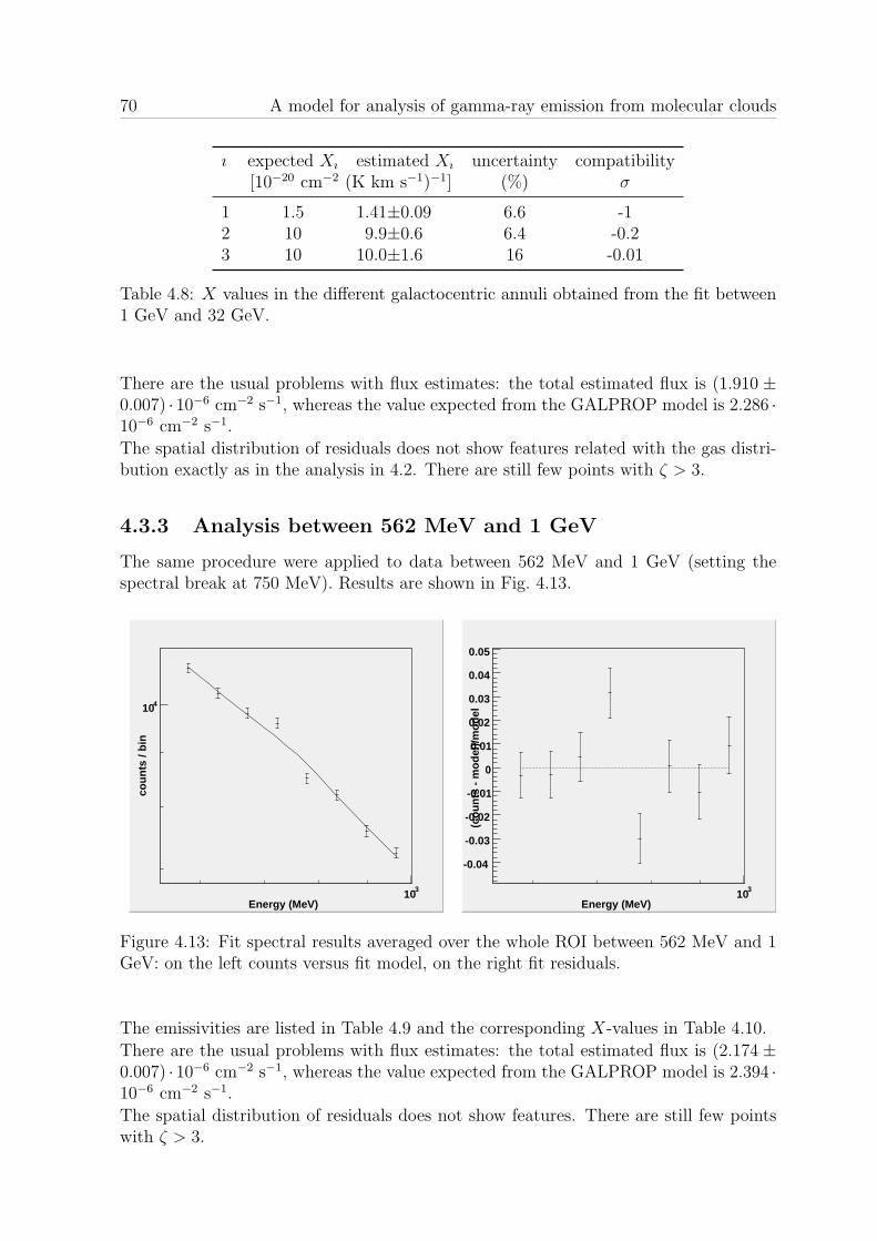
70 A model for analysis of gamma-ray emission from molecular clouds
ı expected Xı estimated Xı uncertainty compatibility[10−20 cm−2 (K km s−1)−1] (%) σ
1 1.5 1.41±0.09 6.6 -12 10 9.9±0.6 6.4 -0.23 10 10.0±1.6 16 -0.01
Table 4.8: X values in the different galactocentric annuli obtained from the fit between1 GeV and 32 GeV.
There are the usual problems with flux estimates: the total estimated flux is (1.910 ±0.007) · 10−6 cm−2 s−1, whereas the value expected from the GALPROP model is 2.286 ·10−6 cm−2 s−1.
The spatial distribution of residuals does not show features related with the gas distri-bution exactly as in the analysis in 4.2. There are still few points with ζ > 3.
4.3.3 Analysis between 562 MeV and 1 GeV
The same procedure were applied to data between 562 MeV and 1 GeV (setting thespectral break at 750 MeV). Results are shown in Fig. 4.13.
Energy (MeV)
310
cou
nts
/ b
in
410
Energy (MeV)
310
(co
un
ts -
mo
del
)/m
od
el
-0.04
-0.03
-0.02
-0.01
0
0.01
0.02
0.03
0.04
0.05
Figure 4.13: Fit spectral results averaged over the whole ROI between 562 MeV and 1GeV: on the left counts versus fit model, on the right fit residuals.
The emissivities are listed in Table 4.9 and the corresponding X-values in Table 4.10.
There are the usual problems with flux estimates: the total estimated flux is (2.174 ±0.007) · 10−6 cm−2 s−1, whereas the value expected from the GALPROP model is 2.394 ·10−6 cm−2 s−1.
The spatial distribution of residuals does not show features. There are still few pointswith ζ > 3.
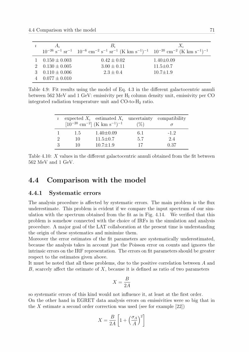
4.4 Comparison with the model 71
ı Aı Bı Xı
10−26 s−1 sr−1 10−6 cm−2 s−1 sr−1 (K km s−1)−1 10−20 cm−2 (K km s−1)−1
1 0.150± 0.003 0.42± 0.02 1.40±0.092 0.130± 0.005 3.00± 0.11 11.5±0.73 0.110± 0.006 2.3± 0.4 10.7±1.94 0.077± 0.010
Table 4.9: Fit results using the model of Eq. 4.3 in the different galactocentric annulibetween 562 MeV and 1 GeV: emissivity per HI column density unit, emissivity per COintegrated radiation temperature unit and CO-to-H2 ratio.
ı expected Xı estimated Xı uncertainty compatibility[10−20 cm−2] (K km s−1)−1 (%) σ
1 1.5 1.40±0.09 6.1 -1.22 10 11.5±0.7 5.7 2.43 10 10.7±1.9 17 0.37
Table 4.10: X values in the different galactocentric annuli obtained from the fit between562 MeV and 1 GeV.
4.4 Comparison with the model
4.4.1 Systematic errors
The analysis procedure is affected by systematic errors. The main problem is the fluxunderestimate. This problem is evident if we compare the input spectrum of our sim-ulation with the spectrum obtained from the fit as in Fig. 4.14. We verified that thisproblem is somehow connected with the choice of IRFs in the simulation and analysisprocedure. A major goal of the LAT collaboration at the present time is understandingthe origin of these systematics and minimize them.Moreover the error estimates of the fit parameters are systematically underestimated,because the analysis takes in account just the Poisson error on counts and ignores theintrinsic errors on the IRF representation. The errors on fit parameters should be greaterrespect to the estimates given above.It must be noted that all these problems, due to the positive correlation between A andB, scarcely affect the estimate of X, because it is defined as ratio of two parameters
X =B
2A
so systematic errors of this kind would not influence it, at least at the first order.On the other hand in EGRET data analysis errors on emissivities were so big that inthe X estimate a second order correction was used (see for example [22])
X =B
2A
[1 +
(σA
A
)2]
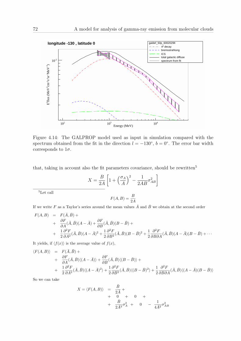
72 A model for analysis of gamma-ray emission from molecular clouds
Energy (MeV)210 310 410
)-1
MeV
-1sr
-1 s-2
cm2fl
ux (
MeV
2E
-210
galdef_50p_6002029lt decay0π
bremsstrahlung
ICStotal galactic diffusespectrum from fit
longitude -130 , latitude 0
Figure 4.14: The GALPROP model used as input in simulation compared with thespectrum obtained from the fit in the direction l = −130, b = 0. The error bar widthcorresponds to 1σ.
that, taking in account also the fit parameters covariance, should be rewritten5
X =B
2A
[1 +
(σA
A
)2
− 1
2ABσ2
AB
]5Let call
F (A,B) =B
2A
If we write F as a Taylor’s series around the mean values A and B we obtain at the second order
F (A,B) = F (A, B) +
+∂F
∂A(A, B)(A− A) +
∂F
∂B(A, B)(B − B) +
+12
∂2F
∂A2(A, B)(A− A)2 +
12
∂2F
∂B2(A, B)(B − B)2 +
12
∂2F
∂B∂A(A, B)(A− A)(B − B) + · · ·
It yields, if 〈f(x)〉 is the average value of f(x),
〈F (A,B)〉 = F (A, B) +
+∂F
∂A(A, B)〈(A− A)〉+
∂F
∂B(A, B)〈(B − B)〉+
+12
∂2F
∂A2(A, B)〈(A− A)2〉+
12
∂2F
∂B2(A, B)〈(B − B)2〉+
12
∂2F
∂B∂A(A, B)〈(A− A)(B − B)〉
So we can take
X = 〈F (A,B)〉 =B
2A+
+ 0 + 0 +
+B
2A3σ2
A + 0 − 14A2
σ2AB
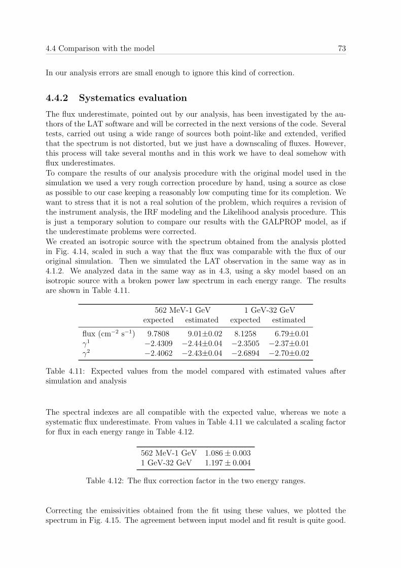
4.4 Comparison with the model 73
In our analysis errors are small enough to ignore this kind of correction.
4.4.2 Systematics evaluation
The flux underestimate, pointed out by our analysis, has been investigated by the au-thors of the LAT software and will be corrected in the next versions of the code. Severaltests, carried out using a wide range of sources both point-like and extended, verifiedthat the spectrum is not distorted, but we just have a downscaling of fluxes. However,this process will take several months and in this work we have to deal somehow withflux underestimates.
To compare the results of our analysis procedure with the original model used in thesimulation we used a very rough correction procedure by hand, using a source as closeas possible to our case keeping a reasonably low computing time for its completion. Wewant to stress that it is not a real solution of the problem, which requires a revision ofthe instrument analysis, the IRF modeling and the Likelihood analysis procedure. Thisis just a temporary solution to compare our results with the GALPROP model, as ifthe underestimate problems were corrected.
We created an isotropic source with the spectrum obtained from the analysis plottedin Fig. 4.14, scaled in such a way that the flux was comparable with the flux of ouroriginal simulation. Then we simulated the LAT observation in the same way as in4.1.2. We analyzed data in the same way as in 4.3, using a sky model based on anisotropic source with a broken power law spectrum in each energy range. The resultsare shown in Table 4.11.
562 MeV-1 GeV 1 GeV-32 GeVexpected estimated expected estimated
flux (cm−2 s−1) 9.7808 9.01±0.02 8.1258 6.79±0.01γ1 −2.4309 −2.44±0.04 −2.3505 −2.37±0.01γ2 −2.4062 −2.43±0.04 −2.6894 −2.70±0.02
Table 4.11: Expected values from the model compared with estimated values aftersimulation and analysis
The spectral indexes are all compatible with the expected value, whereas we note asystematic flux underestimate. From values in Table 4.11 we calculated a scaling factorfor flux in each energy range in Table 4.12.
562 MeV-1 GeV 1.086± 0.0031 GeV-32 GeV 1.197± 0.004
Table 4.12: The flux correction factor in the two energy ranges.
Correcting the emissivities obtained from the fit using these values, we plotted thespectrum in Fig. 4.15. The agreement between input model and fit result is quite good.
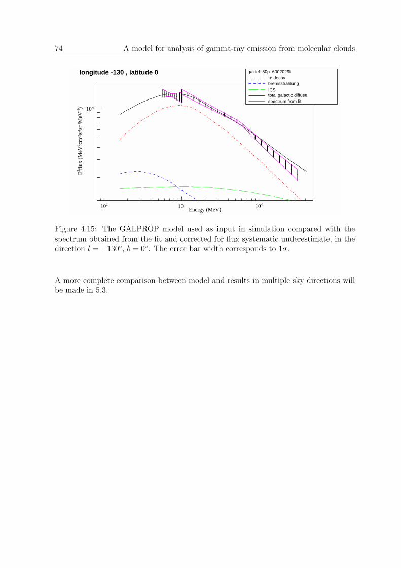
74 A model for analysis of gamma-ray emission from molecular clouds
Energy (MeV)210 310 410
)-1
MeV
-1sr
-1 s-2
cm2fl
ux (
MeV
2E
-210
galdef_50p_6002029lt decay0π
bremsstrahlung
ICStotal galactic diffusespectrum from fit
longitude -130 , latitude 0
Figure 4.15: The GALPROP model used as input in simulation compared with thespectrum obtained from the fit and corrected for flux systematic underestimate, in thedirection l = −130, b = 0. The error bar width corresponds to 1σ.
A more complete comparison between model and results in multiple sky directions willbe made in 5.3.

75
Chapter 5
Analysis of diffuse emission inMonoceros on simulated LAT data
In this chapter we analyze simulated LAT data for a “realistic” sky model of the Mono-ceros region. We start in section 1 with a sky model including the EGRB and pointsources detected by EGRET: we will see that accounting for EGRET point sources isnecessary to correctly estimate emissivities of the interstellar gas and successfully cali-brate the X-ratio. In section 2 we add to the sky model other hypothetical point sources,not detected by EGRET, but that could be seen by the LAT: we find that subtracting thesepoint sources is not strictly needed to study the diffuse emission, although we find someevidence of their presence. In section 3 we compare spectra obtained from our fit withthe GALPROP model used as input in simulation and we discuss the discrepancies, thenwe summarize our results for the X-ratio calibration. Section 4 gives the conclusions ofthis work, illustrating the open issues.
5.1 The EGRET sky model
5.1.1 EGRET sources
The EGRET catalog sources
With respect to the simple sky model used for simulation in chapter 4 we introduced allsources of the third EGRET catalog:
• the galactic diffuse emission modeled as described in 4.1.1;
• the point sources listed in the paper [22], using the DC2 sky model parameters(see Table 5.1);
• the EGRB, as obtained from EGRET data using the optimized GALPROP modelto subtract the galactic diffuse component [56] (see Table 5.2).
The simulation procedure is exactly the same described in 4.1.2.
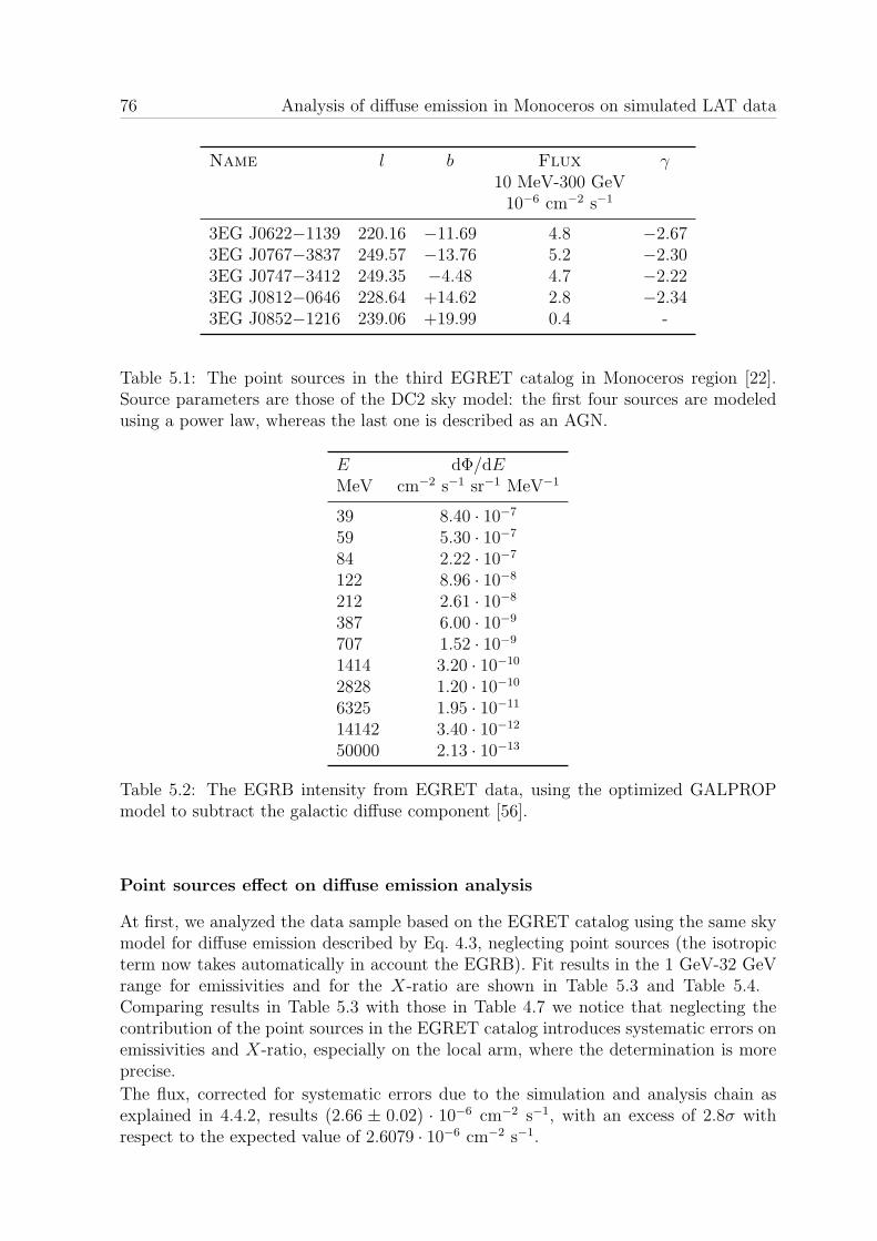
76 Analysis of diffuse emission in Monoceros on simulated LAT data
Name l b Flux γ10 MeV-300 GeV
10−6 cm−2 s−1
3EG J0622−1139 220.16 −11.69 4.8 −2.673EG J0767−3837 249.57 −13.76 5.2 −2.303EG J0747−3412 249.35 −4.48 4.7 −2.223EG J0812−0646 228.64 +14.62 2.8 −2.343EG J0852−1216 239.06 +19.99 0.4 -
Table 5.1: The point sources in the third EGRET catalog in Monoceros region [22].Source parameters are those of the DC2 sky model: the first four sources are modeledusing a power law, whereas the last one is described as an AGN.
E dΦ/dEMeV cm−2 s−1 sr−1 MeV−1
39 8.40 · 10−7
59 5.30 · 10−7
84 2.22 · 10−7
122 8.96 · 10−8
212 2.61 · 10−8
387 6.00 · 10−9
707 1.52 · 10−9
1414 3.20 · 10−10
2828 1.20 · 10−10
6325 1.95 · 10−11
14142 3.40 · 10−12
50000 2.13 · 10−13
Table 5.2: The EGRB intensity from EGRET data, using the optimized GALPROPmodel to subtract the galactic diffuse component [56].
Point sources effect on diffuse emission analysis
At first, we analyzed the data sample based on the EGRET catalog using the same skymodel for diffuse emission described by Eq. 4.3, neglecting point sources (the isotropicterm now takes automatically in account the EGRB). Fit results in the 1 GeV-32 GeVrange for emissivities and for the X-ratio are shown in Table 5.3 and Table 5.4.Comparing results in Table 5.3 with those in Table 4.7 we notice that neglecting thecontribution of the point sources in the EGRET catalog introduces systematic errors onemissivities and X-ratio, especially on the local arm, where the determination is moreprecise.
The flux, corrected for systematic errors due to the simulation and analysis chain asexplained in 4.4.2, results (2.66 ± 0.02) · 10−6 cm−2 s−1, with an excess of 2.8σ withrespect to the expected value of 2.6079 · 10−6 cm−2 s−1.
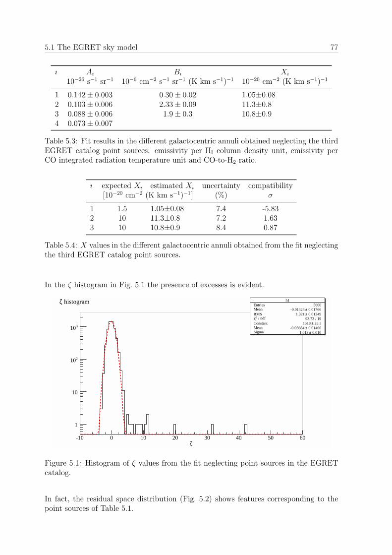
5.1 The EGRET sky model 77
ı Aı Bı Xı
10−26 s−1 sr−1 10−6 cm−2 s−1 sr−1 (K km s−1)−1 10−20 cm−2 (K km s−1)−1
1 0.142± 0.003 0.30± 0.02 1.05±0.082 0.103± 0.006 2.33± 0.09 11.3±0.83 0.088± 0.006 1.9± 0.3 10.8±0.94 0.073± 0.007
Table 5.3: Fit results in the different galactocentric annuli obtained neglecting the thirdEGRET catalog point sources: emissivity per HI column density unit, emissivity perCO integrated radiation temperature unit and CO-to-H2 ratio.
ı expected Xı estimated Xı uncertainty compatibility[10−20 cm−2 (K km s−1)−1] (%) σ
1 1.5 1.05±0.08 7.4 -5.832 10 11.3±0.8 7.2 1.633 10 10.8±0.9 8.4 0.87
Table 5.4: X values in the different galactocentric annuli obtained from the fit neglectingthe third EGRET catalog point sources.
In the ζ histogram in Fig. 5.1 the presence of excesses is evident.
h1Entries 5600Mean 0.01766± -0.01323 RMS 0.01249± 1.321
/ ndf 2χ 93.73 / 19Constant 25.3± 1518 Mean 0.01466± -0.05684 Sigma 0.010± 1.013
ζ-10 0 10 20 30 40 50 60
1
10
210
310
h1Entries 5600Mean 0.01766± -0.01323 RMS 0.01249± 1.321
/ ndf 2χ 93.73 / 19Constant 25.3± 1518 Mean 0.01466± -0.05684 Sigma 0.010± 1.013
histogramζ
Figure 5.1: Histogram of ζ values from the fit neglecting point sources in the EGRETcatalog.
In fact, the residual space distribution (Fig. 5.2) shows features corresponding to thepoint sources of Table 5.1.

78 Analysis of diffuse emission in Monoceros on simulated LAT data
Figure 5.2: On the top counts map (left) versus model map after the fit neglecting theEGRET point sources contribution (right) over the whole energy range. On the bottomthe ζ map: note the features corresponding to point sources in Table 5.1.
5.1.2 Point sources subtraction
After a year of observation we expect that the catalog group within the LAT collabora-tion will have provided a detailed description of all point sources in the LAT sensitivityrange. In this work we did not use the input model to subtract point sources to avoidunderestimates of the stochastic errors. We preferred a more detailed subtraction pro-cedure made by hand: we analyzed each point source on a square region of 3 × 3 inthe range 1 GeV-32 GeV and of 5 × 5 in the range 562 MeV-1 GeV. We modeled allpoint sources (including the AGN J0852−1216) using a power law. Diffuse emission wasdescribed using the EGRET map for the galactic component and an isotropic term forthe EGRB, both with a simple power law spectrum. Results are listed in Table 5.5.
We want to stress that in the real analysis the catalog group will provide a more accuratemodel for point sources, probably reducing the magnitude of errors.
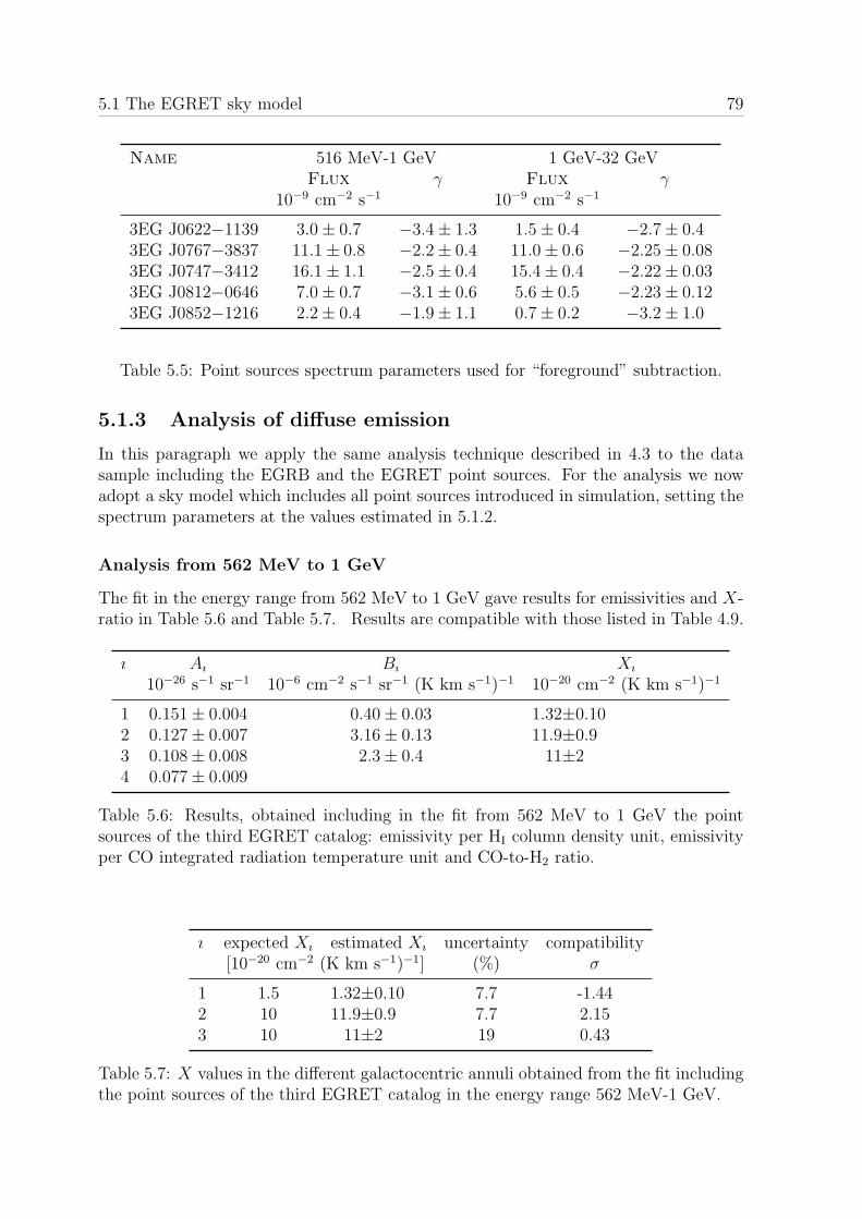
5.1 The EGRET sky model 79
Name 516 MeV-1 GeV 1 GeV-32 GeVFlux γ Flux γ
10−9 cm−2 s−1 10−9 cm−2 s−1
3EG J0622−1139 3.0± 0.7 −3.4± 1.3 1.5± 0.4 −2.7± 0.43EG J0767−3837 11.1± 0.8 −2.2± 0.4 11.0± 0.6 −2.25± 0.083EG J0747−3412 16.1± 1.1 −2.5± 0.4 15.4± 0.4 −2.22± 0.033EG J0812−0646 7.0± 0.7 −3.1± 0.6 5.6± 0.5 −2.23± 0.123EG J0852−1216 2.2± 0.4 −1.9± 1.1 0.7± 0.2 −3.2± 1.0
Table 5.5: Point sources spectrum parameters used for “foreground” subtraction.
5.1.3 Analysis of diffuse emission
In this paragraph we apply the same analysis technique described in 4.3 to the datasample including the EGRB and the EGRET point sources. For the analysis we nowadopt a sky model which includes all point sources introduced in simulation, setting thespectrum parameters at the values estimated in 5.1.2.
Analysis from 562 MeV to 1 GeV
The fit in the energy range from 562 MeV to 1 GeV gave results for emissivities and X-ratio in Table 5.6 and Table 5.7. Results are compatible with those listed in Table 4.9.
ı Aı Bı Xı
10−26 s−1 sr−1 10−6 cm−2 s−1 sr−1 (K km s−1)−1 10−20 cm−2 (K km s−1)−1
1 0.151± 0.004 0.40± 0.03 1.32±0.102 0.127± 0.007 3.16± 0.13 11.9±0.93 0.108± 0.008 2.3± 0.4 11±24 0.077± 0.009
Table 5.6: Results, obtained including in the fit from 562 MeV to 1 GeV the pointsources of the third EGRET catalog: emissivity per HI column density unit, emissivityper CO integrated radiation temperature unit and CO-to-H2 ratio.
ı expected Xı estimated Xı uncertainty compatibility[10−20 cm−2 (K km s−1)−1] (%) σ
1 1.5 1.32±0.10 7.7 -1.442 10 11.9±0.9 7.7 2.153 10 11±2 19 0.43
Table 5.7: X values in the different galactocentric annuli obtained from the fit includingthe point sources of the third EGRET catalog in the energy range 562 MeV-1 GeV.
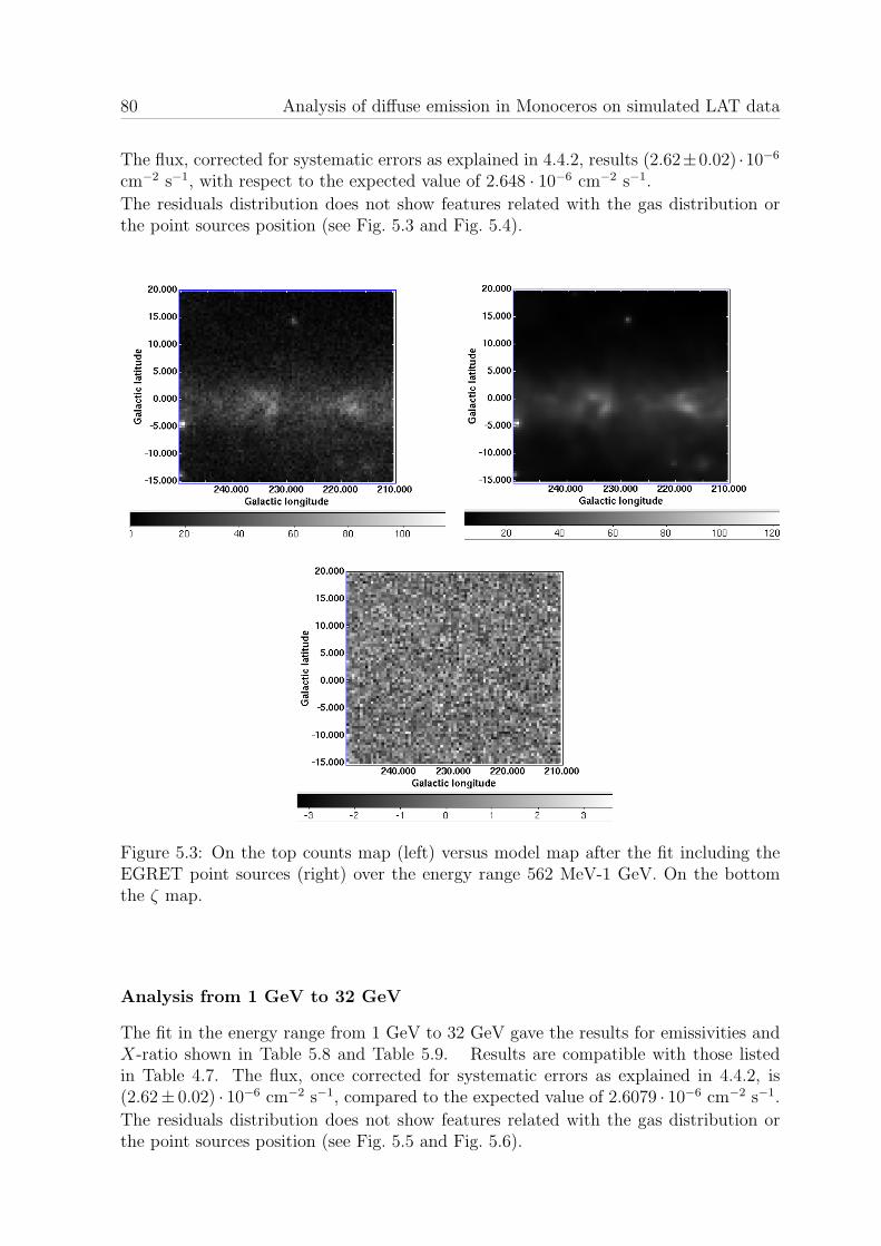
80 Analysis of diffuse emission in Monoceros on simulated LAT data
The flux, corrected for systematic errors as explained in 4.4.2, results (2.62±0.02) ·10−6
cm−2 s−1, with respect to the expected value of 2.648 · 10−6 cm−2 s−1.
The residuals distribution does not show features related with the gas distribution orthe point sources position (see Fig. 5.3 and Fig. 5.4).
Figure 5.3: On the top counts map (left) versus model map after the fit including theEGRET point sources (right) over the energy range 562 MeV-1 GeV. On the bottomthe ζ map.
Analysis from 1 GeV to 32 GeV
The fit in the energy range from 1 GeV to 32 GeV gave the results for emissivities andX-ratio shown in Table 5.8 and Table 5.9. Results are compatible with those listedin Table 4.7. The flux, once corrected for systematic errors as explained in 4.4.2, is(2.62± 0.02) · 10−6 cm−2 s−1, compared to the expected value of 2.6079 · 10−6 cm−2 s−1.
The residuals distribution does not show features related with the gas distribution orthe point sources position (see Fig. 5.5 and Fig. 5.6).
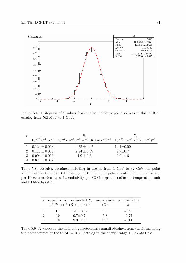
5.1 The EGRET sky model 81
h1Entries 5600Mean 0.01356± 0.00075 RMS 0.009591± 1.015
/ ndf 2χ 119.3 / 32Constant 7.4± 446.9 Mean 0.014400± 0.002164 Sigma 0.0095± 0.9793
ζ-6 -4 -2 0 2 4 6
0
50
100
150
200
250
300
350
400
450
h1Entries 5600Mean 0.01356± 0.00075 RMS 0.009591± 1.015
/ ndf 2χ 119.3 / 32Constant 7.4± 446.9 Mean 0.014400± 0.002164 Sigma 0.0095± 0.9793
histogramζ
Figure 5.4: Histogram of ζ values from the fit including point sources in the EGRETcatalog from 562 MeV to 1 GeV.
ı Aı Bı Xı
10−26 s−1 sr−1 10−6 cm−2 s−1 sr−1 (K km s−1)−1 10−20 cm−2 (K km s−1)−1
1 0.124± 0.003 0.35± 0.02 1.41±0.092 0.115± 0.006 2.24± 0.09 9.7±0.73 0.094± 0.006 1.9± 0.3 9.9±1.64 0.076± 0.007
Table 5.8: Results, obtained including in the fit from 1 GeV to 32 GeV the pointsources of the third EGRET catalog, in the different galactocentric annuli: emissivityper HI column density unit, emissivity per CO integrated radiation temperature unitand CO-to-H2 ratio.
ı expected Xı estimated Xı uncertainty compatibility[10−20 cm−2 (K km s−1)−1] (%) σ
1 1.5 1.41±0.09 6.6 -0.472 10 9.7±0.7 5.8 -0.753 10 9.9±1.6 16.7 -0.14
Table 5.9: X values in the different galactocentric annuli obtained from the fit includingthe point sources of the third EGRET catalog in the energy range 1 GeV-32 GeV.

82 Analysis of diffuse emission in Monoceros on simulated LAT data
Figure 5.5: On the top counts map (left) versus model map including EGRET pointsources (right) over the energy range 1 GeV-32 GeV. On the bottom the ζ map.
h1Entries 5600Mean 0.01374± 7.143e-05 RMS 0.009717± 1.028
/ ndf 2χ 136.5 / 34Constant 7.5± 447.6 Mean 0.01441± -0.00299 Sigma 0.0097± 0.9742
ζ-6 -4 -2 0 2 4 6
0
50
100
150
200
250
300
350
400
450
h1Entries 5600Mean 0.01374± 7.143e-05 RMS 0.009717± 1.028
/ ndf 2χ 136.5 / 34Constant 7.5± 447.6 Mean 0.01441± -0.00299 Sigma 0.0097± 0.9742
histogramζ
Figure 5.6: Histogram of ζ values from the fit including point sources in the EGRETcatalog from 1 GeV to 32 GeV.

5.2 The DC2 sky model 83
5.2 The DC2 sky model
5.2.1 DC2 sources
We continued our test including in the simulation sources not detected by EGRETbut which might be observed by the LAT. The DC2 sky model describes in Monocerosabout a hundred of point sources, part of a population of random generated AGNscalled Giommi blazars1. The less intense source of the EGRET catalog has a flux of0.4·10−6 cm−2 s−1 between 10 MeV and 300 GeV. The additional blazars have intensitiescomparable or lower than this one. We started including in the simulation the 12 mostintense AGNs, described in Table 5.10.
Name RA DEC Flux10 MeV-300 GeV
10−6 cm−2 s−1
Giommi blazar 044 124.80 −11.42 0.59Giommi blazar 049 121.72 +12.10 0.53Giommi blazar 095 116.14 −25.78 0.29Giommi blazar 148 104.10 −42.32 0.28Giommi blazar 163 105.24 −19.01 0.14Giommi blazar 184 119.56 −21.31 0.07Giommi blazar 193 109.47 −8.16 0.19Giommi blazar 208 101.05 −28.56 0.09Giommi blazar 211 126.96 −29.71 0.20Giommi blazar 234 122.82 +7.25 0.15Giommi blazar 235 137.91 −17.32 0.07Giommi blazar 247 96.65 −27.76 0.10
Table 5.10: The 12 most intense sources in Monoceros region in the DC2 sky model,excluding EGRET sources.
In this section we want to understand how much point sources below EGRET sensitivityinfluence the study of diffuse emission and the determination of emissivities and X-ratio.Therefore, we analyzed the data sample including all these sources using for analysis asky model which describes only diffuse emission and point sources in the EGRET catalog,i.e. additional blazars are neglected in analysis while being included in simulation.
5.2.2 Diffuse emission and point sources
Energy range 562 MeV-1 GeV
The fit in the energy range from 562 MeV to 1 GeV gave the results for emissivitiesand X-ratio in Table 5.11 and Table 5.12. Results are compatible with those listed inTable 4.9. The influence of the point sources neglected in the fit on emissivities is not
1Generated using a code developed by Paolo Giommi, Giommi blazars have isotropic spatial distri-bution and redshift and luminosity properties based on multiwavelength observations [25], [34].
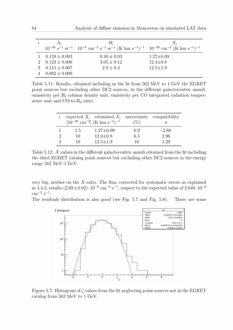
84 Analysis of diffuse emission in Monoceros on simulated LAT data
ı Aı Bı Xı
10−26 s−1 sr−1 10−6 cm−2 s−1 sr−1 (K km s−1)−1 10−20 cm−2 (K km s−1)−1
1 0.159± 0.003 0.40± 0.03 1.27±0.092 0.123± 0.006 3.05± 0.12 12.4±0.83 0.115± 0.007 2.9± 0.4 12.5±1.94 0.082± 0.009
Table 5.11: Results, obtained including in the fit from 562 MeV to 1 GeV the EGRETpoint sources but excluding other DC2 sources, in the different galactocentric annuli:emissivity per HI column density unit, emissivity per CO integrated radiation temper-ature unit and CO-to-H2 ratio.
ı expected Xı estimated Xı uncertainty compatibility[10−20 cm−2] (K km s−1)−1 (%) σ
1 1.5 1.27±0.09 6.9 -2.682 10 12.4±0.8 6.5 2.963 10 12.5±1.9 16 1.29
Table 5.12: X values in the different galactocentric annuli obtained from the fit includingthe third EGRET catalog point sources but excluding other DC2 sources in the energyrange 562 MeV-1 GeV.
very big, neither on the X-ratio. The flux, corrected for systematic errors as explainedin 4.4.2, results (2.69±0.02) ·10−6 cm−2 s−1, respect to the expected value of 2.648 ·10−6
cm−2 s−1.The residuals distribution is also good (see Fig. 5.7 and Fig. 5.8). There are some
h1Entries 5600Mean 0.01404± 0.003875 RMS 0.00993± 1.051 Prob 0Constant 25.1± 1541 Mean 0.0149279± 0.0009732 Sigma 0.0091± 0.9926
ζ-4 -2 0 2 4 6 8
1
10
210
310
h1Entries 5600Mean 0.01404± 0.003875 RMS 0.00993± 1.051 Prob 0Constant 25.1± 1541 Mean 0.0149279± 0.0009732 Sigma 0.0091± 0.9926
histogramζ
Figure 5.7: Histogram of ζ values from the fit neglecting point sources not in the EGRETcatalog from 562 MeV to 1 GeV.
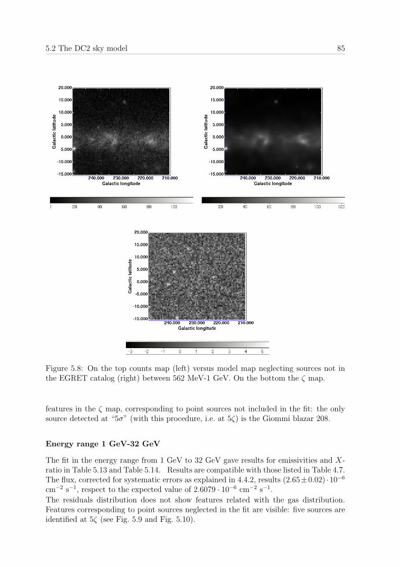
5.2 The DC2 sky model 85
Figure 5.8: On the top counts map (left) versus model map neglecting sources not inthe EGRET catalog (right) between 562 MeV-1 GeV. On the bottom the ζ map.
features in the ζ map, corresponding to point sources not included in the fit: the onlysource detected at “5σ” (with this procedure, i.e. at 5ζ) is the Giommi blazar 208.
Energy range 1 GeV-32 GeV
The fit in the energy range from 1 GeV to 32 GeV gave results for emissivities and X-ratio in Table 5.13 and Table 5.14. Results are compatible with those listed in Table 4.7.The flux, corrected for systematic errors as explained in 4.4.2, results (2.65±0.02) ·10−6
cm−2 s−1, respect to the expected value of 2.6079 · 10−6 cm−2 s−1.
The residuals distribution does not show features related with the gas distribution.Features corresponding to point sources neglected in the fit are visible: five sources areidentified at 5ζ (see Fig. 5.9 and Fig. 5.10).
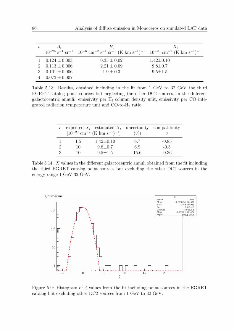
86 Analysis of diffuse emission in Monoceros on simulated LAT data
ı Aı Bı Xı
10−26 s−1 sr−1 10−6 cm−2 s−1 sr−1 (K km s−1)−1 10−20 cm−2 (K km s−1)−1
1 0.124± 0.003 0.35± 0.02 1.42±0.102 0.113± 0.006 2.21± 0.09 9.8±0.73 0.101± 0.006 1.9± 0.3 9.5±1.54 0.073± 0.007
Table 5.13: Results, obtained including in the fit from 1 GeV to 32 GeV the thirdEGRET catalog point sources but neglecting the other DC2 sources, in the differentgalactocentric annuli: emissivity per HI column density unit, emissivity per CO inte-grated radiation temperature unit and CO-to-H2 ratio.
ı expected Xı estimated Xı uncertainty compatibility[10−20 cm−2 (K km s−1)−1] (%) σ
1 1.5 1.42±0.10 6.7 -0.832 10 9.8±0.7 6.9 -0.33 10 9.5±1.5 15.6 -0.36
Table 5.14: X values in the different galactocentric annuli obtained from the fit includingthe third EGRET catalog point sources but excluding the other DC2 sources in theenergy range 1 GeV-32 GeV.
h1Entries 5600Mean 0.01535± -0.003625 RMS 0.01085± 1.148 Prob 2.512e-12Constant 25.1± 1507 Mean 0.01476± -0.02826 Sigma 0.010± 1.021
ζ-5 0 5 10 15 20
1
10
210
310
h1Entries 5600Mean 0.01535± -0.003625 RMS 0.01085± 1.148 Prob 2.512e-12Constant 25.1± 1507 Mean 0.01476± -0.02826 Sigma 0.010± 1.021
histogramζ
Figure 5.9: Histogram of ζ values from the fit including point sources in the EGRETcatalog but excluding other DC2 sources from 1 GeV to 32 GeV.

5.3 Comparison with the model 87
Figure 5.10: On the top counts map (left) versus model map after the fit includingthe EGRET point sources but neglecting the other DC2 sources (right) over the energyrange 1 GeV-32 GeV. On the bottom the ζ map.
Because neglecting in analysis sources detectable by LAT in two months do not influencethe study of the gas-related emission, we did not go ahead with a more accurate skymodel including sources detectable in one year.
5.3 Comparison with the model
5.3.1 The reconstructed spectrum
Now we want to compare the spectrum obtained from our fits with the GALPROPmodel used as input in simulation. Of course we cannot separate the EGRB from the
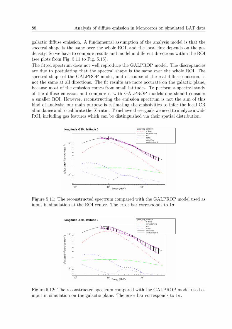
88 Analysis of diffuse emission in Monoceros on simulated LAT data
galactic diffuse emission. A fundamental assumption of the analysis model is that thespectral shape is the same over the whole ROI, and the local flux depends on the gasdensity. So we have to compare results and model in different directions within the ROI(see plots from Fig. 5.11 to Fig. 5.15).
The fitted spectrum does not well reproduce the GALPROP model. The discrepanciesare due to postulating that the spectral shape is the same over the whole ROI. Thespectral shape of the GALPROP model, and of course of the real diffuse emission, isnot the same at all directions. The fit results are more accurate on the galactic plane,because most of the emission comes from small latitudes. To perform a spectral studyof the diffuse emission and compare it with GALPROP models one should considera smaller ROI. However, reconstructing the emission spectrum is not the aim of thiskind of analysis: our main purpose is estimating the emissivities to infer the local CRabundance and to calibrate theX-ratio. To achieve these goals we need to analyze a wideROI, including gas features which can be distinguished via their spatial distribution.
Energy (MeV)210 310 410
)-1
MeV
-1sr
-1 s-2
cm2fl
ux (
MeV
2E -310
-210
galdef_50p_6002029lt decay0π
bremsstrahlungICSEGRBtotal diffusespectrum from fit
longitude -130 , latitude 0
Figure 5.11: The reconstructed spectrum compared with the GALPROP model used asinput in simulation at the ROI center. The error bar corresponds to 1σ.
Energy (MeV)210 310 410
)-1
MeV
-1sr
-1 s-2
cm2fl
ux (
MeV
2E
-310
-210
galdef_50p_6002029lt decay0π
bremsstrahlungICSEGRBtotal diffusespectrum from fit
longitude -120 , latitude 0
Figure 5.12: The reconstructed spectrum compared with the GALPROP model used asinput in simulation on the galactic plane. The error bar corresponds to 1σ.
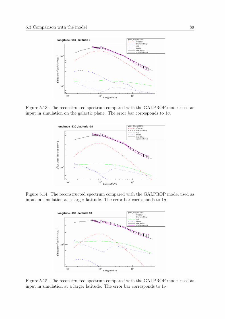
5.3 Comparison with the model 89
Energy (MeV)210 310 410
)-1
MeV
-1sr
-1 s-2
cm2fl
ux (
MeV
2E
-310
-210
galdef_50p_6002029lt decay0π
bremsstrahlungICSEGRBtotal diffusespectrum from fit
longitude -140 , latitude 0
Figure 5.13: The reconstructed spectrum compared with the GALPROP model used asinput in simulation on the galactic plane. The error bar corresponds to 1σ.
Energy (MeV)210 310 410
)-1
MeV
-1sr
-1 s-2
cm2fl
ux (
MeV
2E
-310
galdef_50p_6002029lt decay0π
bremsstrahlungICSEGRBtotal diffusespectrum from fit
longitude -130 , latitude -10
Figure 5.14: The reconstructed spectrum compared with the GALPROP model used asinput in simulation at a larger latitude. The error bar corresponds to 1σ.
Energy (MeV)210 310 410
)-1
MeV
-1sr
-1 s-2
cm2fl
ux (
MeV
2E
-310
galdef_50p_6002029lt decay0π
bremsstrahlungICSEGRBtotal diffusespectrum from fit
longitude -130 , latitude 10
Figure 5.15: The reconstructed spectrum compared with the GALPROP model used asinput in simulation at a larger latitude. The error bar corresponds to 1σ.
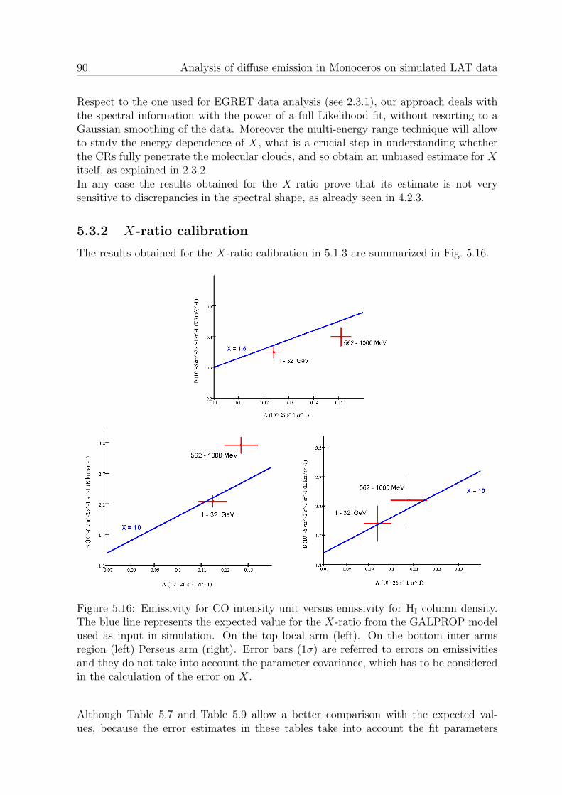
90 Analysis of diffuse emission in Monoceros on simulated LAT data
Respect to the one used for EGRET data analysis (see 2.3.1), our approach deals withthe spectral information with the power of a full Likelihood fit, without resorting to aGaussian smoothing of the data. Moreover the multi-energy range technique will allowto study the energy dependence of X, what is a crucial step in understanding whetherthe CRs fully penetrate the molecular clouds, and so obtain an unbiased estimate for Xitself, as explained in 2.3.2.In any case the results obtained for the X-ratio prove that its estimate is not verysensitive to discrepancies in the spectral shape, as already seen in 4.2.3.
5.3.2 X-ratio calibration
The results obtained for the X-ratio calibration in 5.1.3 are summarized in Fig. 5.16.
Figure 5.16: Emissivity for CO intensity unit versus emissivity for HI column density.The blue line represents the expected value for the X-ratio from the GALPROP modelused as input in simulation. On the top local arm (left). On the bottom inter armsregion (left) Perseus arm (right). Error bars (1σ) are referred to errors on emissivitiesand they do not take into account the parameter covariance, which has to be consideredin the calculation of the error on X.
Although Table 5.7 and Table 5.9 allow a better comparison with the expected val-ues, because the error estimates in these tables take into account the fit parameters
5.3 Comparison with the model 91
covariance, Fig. 5.16 leads to consider that the X-ratio has been successfully calibrated.Once hopefully extended the analysis at lower energies, this kind of plot will be fun-damental to understand if there is an energy dependence of the X estimate, hint ofan incomplete penetration of CRs into molecular clouds. This will allow an unbiasedconversion between CO emission intensity and H2 column density (see 2.3.1).
92 Analysis of diffuse emission in Monoceros on simulated LAT data
5.4 Conclusions
This thesis presents a procedure for LAT data analysis of diffuse γ-rays from molecularclouds. Thanks to the improved capabilities of the GLAST LAT with respect to theprevious γ-ray telescopes, this model lets us use a Likelihood fit to separate emissionfrom gas at different distances from the galactic center, leading to estimate the local γ-ray emissivity (and so qualitatively the local cosmic ray abundance) in different regionswith a ∼ 5% error. Moreover the emissivity values allow to experimentally calibrate theconversion factor X between the CO emission intensity in the radio domain and the H2
column density beyond the Solar circle with a . 20% error.
The analysis model has been tested on simulated LAT data:
• the isotropic approximation for IC emission can be used, without affecting ourresults, to avoid a model-dependent subtraction and use the results themselves torefine the diffuse emission models;
• intense point-like sources and the EGRB (the latter included into the isotropicterm which describes the IC emission as well) can be easily subtracted to studythe diffuse emission from the interstellar gas;
• fainter point sources, even if identified in the analysis procedure, scarcely affectthe determination of the emissivities;
• the local power law approximation in a multi-energy range analysis procedure al-lows to roughly reconstruct the emission spectrum and to compare it with physicalmodels;
• the uncertainties on the spectral behavior do not significantly affect the estimateof the emissivities and the X-ratio.
There are still some open issues:
• the use of IRFs in the analysis procedure is somehow connected with flux under-estimates; this systematic errors should be minimized through a revision of theinstrument analysis, the IRF modeling and the IRF convolution in the Likelihoodanalysis2;
• the analysis method is not effective at low energies (. 500 MeV) due to the worsePSF which does not allow to separate the emission from gas at different galacto-centric radii using its spatial distribution; the problem might be overcome using adedicated set of analysis cuts and IRFs for diffuse emission with an improved PSFat low energies;
• an accurate analysis should investigate effects of the choice of energy ranges to beused on the results;
2In fact the flux underestimate was mostly due to a bug in the simulation tool, corrected afterwriting this thesis.
5.4 Conclusions 93
• this work does not consider the charged background, which could affect this kindof analysis requiring long observations (at least of ∼1 year); due to computingdifficulties in simulating the charged background, a detailed comprehension of thephenomenon will be possible only when GLAST is on orbit.
Although there are still some open questions, perspectives for studying the diffuse emis-sion from molecular clouds on the GLAST LAT data are exciting. The CO-to-H2 con-version factor, once experimentally calibrated through this phenomenon, will be fixedwithin the diffuse γ-ray emission models. At this point the comparison between LATdata and models, together with the emissivity values estimated in molecular cloudsanalysis itself, will allow to greatly improve our knowledge of the cosmic ray sourcesdistribution and propagation mechanisms. Combining these results with observations ofγ-ray emission from CR acceleration sites will lead to a comprehension without prece-dent of the cosmic ray acceleration and propagation in the Galaxy.
94
Appendix A
Theoretical elements about cosmicray propagation and acceleration
This appendix contains some theoretical elements on CR acceleration and propagation.A complete review of this subject can be found in [30] and [50], in this appendix we willdiscuss some concepts useful to understand 2.2.1.Most of the non stellar matter in the Universe is ionized. An electrically neutral systemof charged and neutral particles interacting so much that their collective Lorentz forcesinfluence the properties of the medium considerably is referred to as a plasma. Plasmasin space, including CRs, can be considered collision-free. The collision frequency ν =vnσ for electrons can be calculated assuming that the cross section σ is given by theshortest distance allowed by Coulomb interaction taken in account the kinetic energy ofthe pair. It yields
νee =g
3ωpe
where ωpe is the electron plasma frequency (in Gauss units)
ωpe =
(4πe2ne
me
)2
and g = 1/Ns is the opposite of the number of charges electromagnetically interacting(not shielded by collective forces) in a Debye sphere
Ns =4π
3neλ
3De =
4π
3ne
(kBTe
4πnee2
)3/2
For the existence of a plasma there are two requirements: the physical dimensions ofthe system have to be larger than the Debye length λDe and Ns has to be very large, sog very small. Therefore
νee =g
3ωpe ωpe
The electron-ion and ion-ion collision frequencies are smaller than the electron-electronone, so we can conclude that the astrophysical plasma is essentially collisionless.The dynamics of a plasma is described by the Vlasov equation for the distributionfunction f of charged particles and Mawell’s equations for electromagnetic field ( ~E, ~B).No solution exists for this nonlinear problem: if we assume an equilibrium solution
CR propagation and acceleration 95
(f (0), ~E0, ~B0) we can linearize the system and look for solutions in term of perturbations
(δf, δ ~E, δ ~B).For a given charged particle distribution function, solutions for field equations are plasmawaves with the dispersion relation
k2c2
ω2=
(c
vA
)2Ωp
(Ωp − ω)
where vA is the Alfven velocity
vA =B0√
4π(mp +me)ne
and Ωp is the proton gyrofrequency
Ωp =eB0
mpc
which describes the rotation frequency of a proton in the background magnetic field.For small wavenumbers we have non dispersive Alfven waves
ω± ' ±vAk
whereas for large wavenumbers we have the ion cyclotron wave and the whistler wave
ω+ ' +Ωp ω− ' −(v2
Ak2
Ωp
+ Ωp
)For a given electromagnetic field the response of the charged particles can be describedagain in term of a plasma wave. Waves propagating along the magnetic field have thelargest growth rate, so we can assume as a first approximation that wave vectors offluctuations are all parallel to the background magnetic field (slab turbulence).The slab Alfven waves dominate the CR propagation: we can split the particle distri-bution function into its average in pitch angle respect to the magnetic field (let say the~x direction) and in an anisotropic part. The anisotropy is made up of two components,the first one related to the spatial gradient of the distribution function, the second oneto the momentum gradient. The anisotropy can be expanded into Legendre polyno-mials, defining the harmonics Al. At the second order the Vlasov equation yields thediffusion-convection transport equation
∂f
∂t− S(~r, ~p, t) = ∇ · (κxx
~∇f)−∇ ·[(
~U +1
4p2
∂
∂p(p2~vA1)
)f
]+
+1
p2
∂
∂p
(p2A2
∂f
∂p
)+
[p
3
∂~U
∂x+~v
4
]· ~∇A1
∂f
∂p(A.1)
where S is the source term, κxx the diffusion coefficient, ~v the particle speed and ~U isthe bulk speed of the plasma respect to the observer. In Eq. A.1 the first line gives thespatial diffusion and convection terms, the second one gives the momentum diffusionand convection terms, usually known as Fermi second order and Fermi first order term.
96 CR propagation and acceleration
The Fermi first order mechanism is the most likely CR acceleration mechanism. Intenuous astrophysical plasmas typical sounds speeds are considerably less than easilyobtainable bulk flows velocities, and shocks are expected to develop. Different calcula-tions show that a power law spectrum of particle momentum results from very generalproperties of collisionless shock acceleration (see for example [9]). The Fermi accelera-tion might take place in different sites, such as SNRs and XRBs (see 1.3).
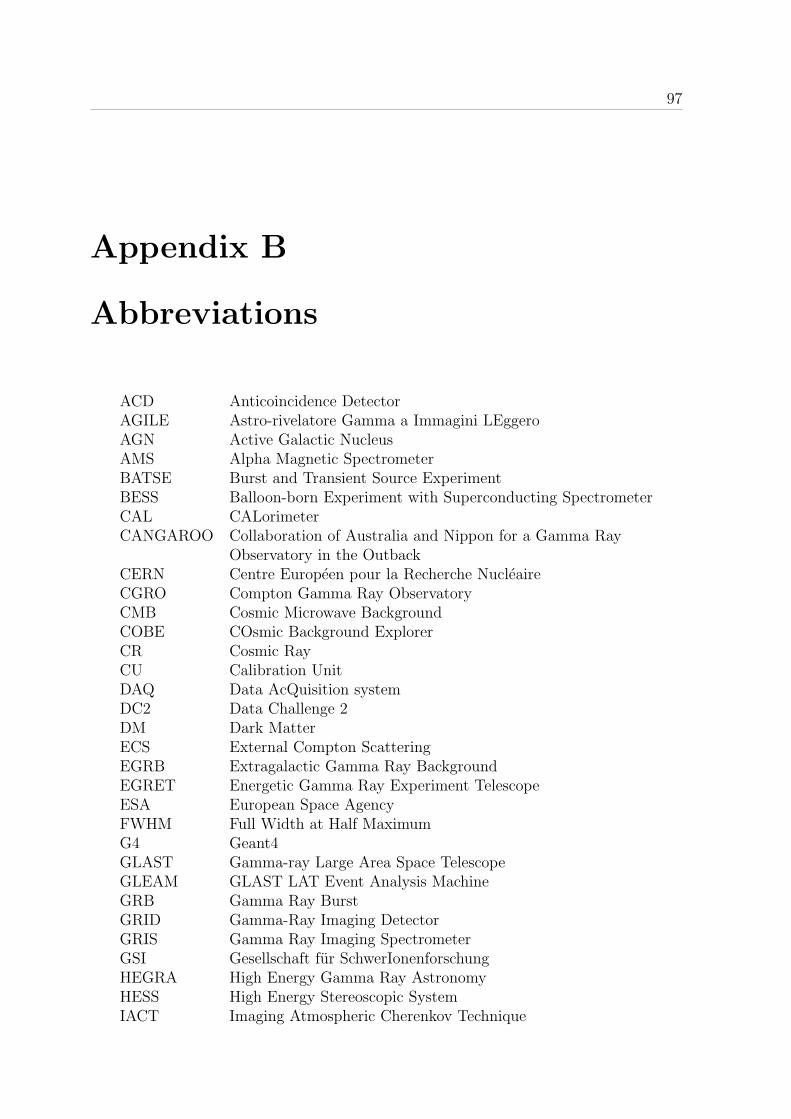
97
Appendix B
Abbreviations
ACD Anticoincidence DetectorAGILE Astro-rivelatore Gamma a Immagini LEggeroAGN Active Galactic NucleusAMS Alpha Magnetic SpectrometerBATSE Burst and Transient Source ExperimentBESS Balloon-born Experiment with Superconducting SpectrometerCAL CALorimeterCANGAROO Collaboration of Australia and Nippon for a Gamma Ray
Observatory in the OutbackCERN Centre Europeen pour la Recherche NucleaireCGRO Compton Gamma Ray ObservatoryCMB Cosmic Microwave BackgroundCOBE COsmic Background ExplorerCR Cosmic RayCU Calibration UnitDAQ Data AcQuisition systemDC2 Data Challenge 2DM Dark MatterECS External Compton ScatteringEGRB Extragalactic Gamma Ray BackgroundEGRET Energetic Gamma Ray Experiment TelescopeESA European Space AgencyFWHM Full Width at Half MaximumG4 Geant4GLAST Gamma-ray Large Area Space TelescopeGLEAM GLAST LAT Event Analysis MachineGRB Gamma Ray BurstGRID Gamma-Ray Imaging DetectorGRIS Gamma Ray Imaging SpectrometerGSI Gesellschaft fur SchwerIonenforschungHEGRA High Energy Gamma Ray AstronomyHESS High Energy Stereoscopic SystemIACT Imaging Atmospheric Cherenkov Technique

98 Abbreviations
IBIS Imager on Board of the INTEGRAL SatelliteIC Inverse ComptonICRC International Cosmic Ray ConferenceICS Inverse Compton ScatteringINTEGRAL INTErnational Gamma Ray Astrophysics LaboratoryIR InfraRedIRAS InfraRed Astronomical SatelliteIRF Instrument Response FunctionISM InterStellar MediumISRF InterStellar Radiation FieldL1T Level 1 TriggerL2T Level 2 TriggerL3T Level 3 TriggerLANL Los Alamos National LaboratoriesLAT Large Area TelescopeLHC Large Hadron ColliderLSP Lightest Super PartnerMAGIC Major Atmospheric Gamma Imaging CherenkovMIP Minimum Ionizing ParticleNASA National Aeronautics and Space AdministrationOSSE Oriented Scintillation-Spectrometer ExperimentPAMELA Payload for Antimatter Matter Exploration and Light nuclei
AstrophysicsPMT PhotoMultiplier TubePS Proton SynchrotronPSF Point Spread FunctionPSR PulSaRROI Region Of InterestSAA South Atlantic AnomalySIU Spacecraft Interface UnitSMM Solar-Maximum MissionSN SuperNovaSNR SuperNova RemnantSPI SPectrometer on IntegralSPS Super Proton SynchrotronSSC Synchrotron Self ComptonSSD Silicon Strip DetectorSSR Solid State RecorderSUSY SUperSYmmetric theoryTEM Tower Electronic ModulesTKR TracKeRUV UltraVioletVERITAS Very Energetic Radiation Imaging Telescope Array SystemWIMP Weakly Interacting Massive ParticleWSF Wavelength Shifting FibersXRB X-Ray Binary
99
Bibliography
[1] NASA GLAST official web site, http://glast.gsfc.nasa.gov/.
[2] Stanford GLAST web site, http://glast.stanford.edu/.
[3] GLAST at the Stanford Linear Accelerator Center,http://glast.slac.stanford.edu/.
[4] GLAST LAT software user workbook,http://glast-ground.slac.stanford.edu/workbook/.
[5] Aous A. Abdo et al., Discovery of TeV gamma-ray emission from the Cygnus regionof the Galaxy, The Astrophysical Journal, 658, L33, 2007.
[6] Carmen Baixeras et al., The MAGIC telescope, Nuclear Physics B, 114, 247, 2003.
[7] David L. Band et al., The statistics of the search for absorption lines in burstspectra, AIP Conference Proceedings, 384, 1996.
[8] Gianfranco Bertone et al., Particle Dark Matter: evidence, candidates and con-straints, hep-ph/0404175v2, 2004.
[9] Roger D. Blandford and James P. Ostriker, Particle acceleration by astrophysicalshocks, The Astrophysical Journal, 221, L29, 1978.
[10] J. B. G. M. Blomen et al., Gamma rays from atomic and molecular gas in the largecomplex of clouds in Orion and Monoceros, Astronomy and Astrophysics, 139, 37,1984.
[11] Praveen Boinee et al., GLEAM: the GLAST Large Area Telescope SimulationFramework, in Stefano Ciprini et al., Proceedings of Science with new generation ofhigh energy gamma-ray experiments, Perugia, 2003.
[12] Richard R. Burman, Flux conservation, Magnetohydrodynamic and force-free ap-proximations for relativistically streaming plasmas, Australian Journal of Physics,31, 523, 1978.
[13] Werner Collmar, Gamma-ray emission of active galaxies, A.A.V.V., The Universein gamma rays, Berlin Heidelberg, 2001.
[14] Werner Collmar, X-ray binaries as gamma-ray sources, A.A.V.V., The Universe ingamma rays, Berlin Heidelberg, 2001.
100 Bibliography
[15] James M. Cordes, The galactic distribution of free electrons, Nature, 354, 121,1991.
[16] James W. Cronin, Cosmic rays: the most energetic particles in the Universe, Re-views of Modern Physics, 71, 1999.
[17] Thomas M. Dame et al., The Milky Way in molecular clouds: a new complete COsurvey, The Astrophisical Journal, 547, 792, 2001.
[18] Robert L. Dickman, The ratio of Carbon monoxide to molecular Hydrogen in inter-stellar dark clouds, The Astrophysical Journal Supplement Series, 37, 407, 1978.
[19] Roland Diehl, Gamma-ray production and absorption processes, A.A.V.V., TheUniverse in gamma rays, Berlin Heidelberg, 2001.
[20] Seth W. Digel et al., EGRET observations of gamma-ray emission from the inter-stellar gas in Orion, The Astrophysical Journal, 441, 270, 1995.
[21] Seth W. Digel et al., Diffuse high-energy gamma-ray emission beyond the Solarcircle: the Cepheus and Polaris flares and the Perseus arm, The AstrophysicalJournal, 463, 609, 1996.
[22] Seth W. Digel et al., EGRET observations of Monoceros: diffuse gamma-ray emis-sion in the outer Galaxy, The Astrophysical Journal, 555, 12, 2001.
[23] Brenda L. Dingus, Milagro: a TeV gamma-ray monitor of the northern emispheresky, Proceedings of the 5th Compton Symposium, Portsmouth, 1999.
[24] Joseph A. Esposito et al., In-flight calibration of EGRET on the Compton GammaRay Observatory, Astrophysical Journal Supplement Series, 123, 203, 1999.
[25] Paolo Giommi et al., Blazar surveys with WMAP and Swift, in Steven Ritz etal., The first GLAST Symposium, AIP Conference Proceedings, 921, 32, Stanford,2007.
[26] Michael A. Gordon and William B. Burton, Carbon monoxide in the Galaxy. I -The radial distribution of CO, H2, and nucleons, The Astrophysical Journal, 208,346, 1976.
[27] Stanley D. Hunter et al. Gamma-ray observations of Ophiucus with EGRET: thediffuse emission and point sources, The Astrophysical Journal, 436, 216, 1994.
[28] Stanley D. Hunter et al., EGRET observations of the diffuse gamma-ray emissionfrom the galactic plane, The Astrophysical Journal, 481, 205, 1997.
[29] Anatoli Iyudin and Gottfried Kanbach, Continuum gamma ray emission from su-pernova remnants, A.A.V.V., The Universe in gamma rays, Berlin Heidelberg, 2001.
[30] Frank C. Jones and Donald C. Ellison, The Plasma Physics of shock acceleration,Space Science Review, 58, 259, 1991.
Bibliography 101
[31] Gottfried Kanbach, Gamma-ray pulsars, A.A.V.V., The Universe in gamma rays,Berlin Heidelberg, 2001.
[32] Marc L. Kutner and Chung Ming Leung, On the conversion of Carbon monoxideintensities to molecular Hydrogen abundances, The Astrophysical Journal, 291, 188,1985.
[33] Giselher Lichti and Robert Georgii, Instruments, A.A.V.V., The Universe in gammarays, Berlin Heidelberg, 2001.
[34] Enrico Massaro et al., A Multifrequency Blazar catalog, in The first GLAST Sym-posium, AIP Conference Proceedings, 921, 349, Stanford, 2007.
[35] James R. Mattox, The Likelihood Analysis of EGRET data, The AstrophysicalJournal, 461, 396, 1996.
[36] Julie E. McEnery et al., GLAST, understanding the high energy gamma-ray sky,astro-ph/0406250v1, 2003.
[37] Igor V. Moskalenko and Andrew W. Strong, Production and propagation of cosmic-ray positrons and electrons, The Astrophysical Journal, 493, 694, 1998.
[38] Igor V. Moskalenko and Andrew W. Strong, Anisotropic Inverse Compton Scatter-ing in the Galaxy, The Astrophysical Journal, 528, 357, 2000.
[39] Igor V. Moskalenko et al., Secondary antiprotons and propagation of cosmic rays inthe Galaxy and heliosphere, The Astrophysical Journal, 565, 280, 2002.
[40] Igor V. Moskalenko et al., Evaluation of production cross section of Li, Be, B inCR, astro-ph/0306367v1, 2003.
[41] Igor V. Moskalenko et al., Diffuse gamma rays: galactic and extragalactic diffuseemission, astro-ph/0402243v1, 2004.
[42] Igor V. Moskalenko and Andrew W. Strong, Diffuse gamma-ray emission: lessonsand perspectives, astro-ph/0509414v1, 2005.
[43] Igor V. Moskalenko and Troy A. Porter, Gamma-ray albedo from the Moon, astro-ph/07053856v1, 2007.
[44] Troy A. Porter and Andrew W. Strong, A new estimate of the Galactic interstellarradiation field between 0.1 µm and 1000 µm, Proceedings of the 29th InternationalCosmic Ray Conference, 00, 101, 2005.
[45] Troy A. Porter et al., The diffuse Galactic gamma-ray emission model for GLASTLAT, to be published in the Proceedings of the 30th International Cosmic RayConference, astro-ph/07060221v1, 2007.
[46] Riccardo Rando, The GLAST mission: assessing radiation hardness and perfor-mances of GLAST LAT tracker electronics, PhD thesis, Padova, 2004.
102 Bibliography
[47] Erich Riegel and Gerhard Rank, The Sun as a gamma-ray source, A.A.V.V., TheUniverse in gamma rays, Berlin Heidelberg, 2001.
[48] Marcus Samorski and William Stamm, Detection of 2·1015 to 2·1016 eV gamma-raysfrom Cygnus X-3, The Astrophysical Journal, 268, L17, 1984.
[49] Eun-Suk Seo and Vladimir S. Ptuskin, Stochastic reacceleration of cosmic rays inthe interstellar medium, The Astrophysical Journal, 431, 705, 1994.
[50] Reinhard Schlickeiser, Cosmic Ray Astrophysics, Berlin Heidelberg, 2002.
[51] Carmelo Sgro, Studio e caratterizzazione del tracciatore al Silicio del Large AreaTelescope di GLAST, M.A. thesis, Pisa, 2004.
[52] Andrew W. Strong and Igor V. Moskalenko, Propagation of cosmic-ray nucleons inthe Galaxy, The Astrophysical Journal, 509, 212, 1998.
[53] Andrew W. Strong et al., Diffuse continuum gamma rays from the Galaxy, TheAstrophysical Journal, 537, 2000.
[54] Andrew W. Strong et al., Diffuse galactic continuum gamma rays: a model compat-ible with EGRET data and cosmic-ray measurements, The Astrophysical Journal,613, 962, 2004.
[55] Andrew W. Strong et al., The distribution of cosmic ray sources in the Galaxy,γ-rays and the gradient in CO-to-H2 relation, Astronomy and Astrophysics, 422,L47, 2004.
[56] Andrew W. Strong et al., A new determination of the extragalactic diffuse gamma-ray background from EGRET data, The Astrophysical Journal, 613, 956, 2004.
[57] Andrew W. Strong and Igor V. Moskalenko, GALPROP C++ v.50: ExplanatorySupplement, http://galprop.stanford.edu/manuals/manual.pdf, 2006.
[58] David J. Thompson, Gamma ray pulsars multiwavelength observations, astro-ph/0312272v1, 2003.
[59] Megan Urry and Paolo Padovani, Unified schemes for radio-loud Active GalacticNuclei, Publications of the Astronomical Society of the Pacific, 107, 803, 1995.
[60] Jacques P. Vallee, Observations of the magnetic fields inside and outside the MilkyWay, starting with globules (∼1 parsec), filaments, clouds, superbubbles, spiralarms, galaxies, superclusters, and ending with the cosmological Universe’s back-ground surface (at ∼8 Teraparsecs), Fundamentals of Cosmic Physics, 19, 1, 1997.
[61] Martin Varendorff, Gamma-ray bursts, A.A.V.V., The Universe in gamma rays,Berlin Heidelberg, 2001.
[62] Richard J. Wainscoat et al., A model of the 8-25 micron point source infrared sky,The Astrophysical Journal Supplements, 83, 111, 1992.
103
Acknowledgments
And I become older always learning many things.
Solon, VI b.C.
First of all I am deeply indebted to Giovanni Busetto who introduced me to the GLASTmission, supervised me during my thesis work and always gives me precious suggestionsthanks to his great experience in Physics. I gratefully acknowledge Riccardo Rando:during the last two and a half years he guided me holding my hand through all difficultiesI had in my work and taught me to carry out research with humility and patience. Mythanks to Denis Bastieri for his helpful comments on my thesis and to all other peoplein the GLAST group of Padova. My acknowledgments to the guys of the electroniclaboratory who gave me hospitality until June: Serena, Jeff, Devis, Mario, Andrea andPiero.I acknowledge the great support from the Diffuse and Molecular Clouds Science group ofthe GLAST collaboration. Thanks to Troy Porter, the coordinator, for his suggestionsand the opportunity of presenting my work to the collaboration. My acknowledgmentsto Andrew Strong, Igor Moskalenko and all other people who contributed to the devel-opment of GALPROP, a masterpiece in Cosmic Ray Science. I especially thank SethDigel who carefully supervised me when I was at SLAC as a summer student and hasnever stopped helping me with my work.I am indebted to my teachers and my course-mates, especially Alessandro Venturini,who read my thesis and gave me interesting hints. I acknowledge the support that Ihave been receiving from all my friends for five years, in a special way the people I metin the Collegio don Mazza, my home here in Padova. My thanks to all my family andto my parents, for so much, my love.During the last five years I was given so much, not just as a physicist: I acknowledge allpeople I learnt something from (they are a lot and, of course, they are not all mentionedin this list) and I hope I will keep discovering something new everyday in my life.

104
Ringraziamenti
E invecchio sempre molte cose imparando.
Solone, VI a.C.
Innanzitutto ringrazio Giovanni Busetto che mi ha permesso di conoscere GLAST, miha fatto da relatore e mi da sempre preziosi consigli in virtu della sua grande esperienzacome fisico. Ringrazio con riconoscenza Riccardo Rando: durante gli ultimi due annie mezzo mi ha condotto per mano attraverso tutte le difficolta che ho incontrato nelmio lavoro e mi ha insegnato come si fa ricerca con umilta e pazienza. Grazie a DenisBastieri per i suoi utili commenti sulla mia tesi e a tutte le altre persone del gruppoGLAST di Padova. Grazie anche ai ragazzi del laboratorio di elettronica che mi hannodato ospitalita fino a Giugno: Serena, Jeff, Devis, Mario, Andrea e Piero.Ringrazio per il sostegno ricevuto il gruppo Diffuse and Molecular Clouds all’internodella collaborazione GLAST. Grazie al coordinatore Troy Porter per i suoi consigli e perla possibilita di presentare il mio lavoro alla collaborazione. La mia riconoscenza va adAndrew Strong, Igor Moskalenko e tutti gli altri che hanno contribuito allo sviluppo diGALPROP, un capolavoro nella scienza dei raggi cosmici. Ringrazio in particolare SethDigel che mi ha fatto con attenzione da supervisore nell’estate che ho trascorso a SLACe non ha mai smesso di aiutarmi nel mio lavoro.Ringrazio i miei insegnanti e i miei compagni di corso, in particolare Alessandro Ventu-rini, che ha letto la tesi e mi ha dato interessanti suggerimenti. La mia riconoscenza vaa tutti i miei amici per il sostegno ricevuto durante i cinque anni che ho impiegato perraggiungere la laurea, in modo particolare alle persone che ho incontrato nel Collegiodon Mazza, la mia casa qui a Padova. Un ringraziamento alla mia famiglia e ai mieigenitori, per avermi dato cosı tanto, tutto il mio affetto.Gli ultimi cinque anni mi hanno dato molto, non solo dal punto di vista della Fisica:ringrazio tutti quelli da cui ho imparato qualcosa (sono tanti e, ovviamente non sonotutti citati nella lista) sperando di continuare a scoprire qualcosa di nuovo ogni giornodella mia vita.