Simple computer code for estimating cosmic-ray shieldingby oddly shaped objects

Greg Balcoa,∗

a Berkeley Geochronology Center, 2455 Ridge Road, Berkeley CA 94709 USA

Abstract

This paper describes computer code for estimating the effect on cosmogenic-nuclideproduction rates of arbitrarily shaped obstructions that partially or completely attenuatethe cosmic ray flux incident on a sample site. This is potentially useful for cosmogenic-nuclide exposure dating of geometrically complex landforms. The code has been vali-dated against analytical formulae applicable to objects with regular geometries. It hasnot yet been validated against empirical measurements of cosmogenic-nuclide concen-trations in samples with the same exposure history but different shielding geometries.

Keywords: Cosmogenic nuclide geochemistry, Exposure-age dating, Monte Carlointegration, Precariously balanced rocks

1. Importance of geometric shielding of the cosmic-ray flux to exposure dating

Cosmogenic-nuclide exposure dating is a geochemical method used to determinethe age of geological events that modify the Earth’s surface, such as glacier advancesand retreats, landslides, earthquake surface ruptures, or instances of erosion or sedi-ment deposition. To determine the exposure age of a rock surface, one must i) measurethe concentration of a trace cosmic-ray-produced nuclide (e.g., 10Be, 26Al, 3He, etc.);and ii) use an independently calibrated nuclide production rate to interpret the concen-tration as an exposure age (see review in Dunai, 2010).

Typically (Dunai, 2010), estimating the production rate at a sample site employssimplifying assumptions that i) the sample is located on an infinite flat surface; ii) allcosmic rays responsible for nuclide production originate from the upper hemisphere;and ii) any topographic obstructions to the cosmic-ray flux can be represented as anapparent horizon below which cosmic rays are fully obstructed, and above which theyare fully admitted (the ‘opaque-horizon’ assumption). These assumptions are adequatefor a wide range of useful exposure-dating applications, but they fail for sample siteslocated on irregular surfaces with a roughness scale similar to the characteristic cosmicray attenuation length in rock (order 1 meter), or likewise for sample sites located onor near meter-scale boulders or other objects.

∗Corresponding author. Tel. 510.644.9200 Fax 510.644.9201Email address: balcs@bgc.org (Greg Balco )

Preprint submitted to Quaternary Geochronology December 23, 2013

The opaque-horizon assumption fails in these situations for two reasons. First, rockis denser than air. Attenuation of cosmic rays is proportional to the amount of massthey travel through. Thus, if cosmic rays must penetrate both the overlying atmosphereand also some additional thickness of rock (or any massive material, e.g., soil, sedi-ment, water, etc.) to reach a sample site, then the production rate at that site will beless than it would be in the reference case of an infinite flat surface (where cosmicrays only travel through air to reach the sample site). If the thickness of rock traversedis much longer than the cosmic-ray attenuation length (e.g., tens of meters or more),then the cosmic-ray flux from that direction is completely attenuated and the opaque-horizon assumption is adequate. However, if it is relatively short (order 1 meter) thenthe cosmic-ray flux is only partially attenuated and this assumption fails. This effectis referred to in this paper as ‘geometric shielding.’ The term ‘self-shielding’ is some-times used to describe this effect, although that term is somewhat misleading becauseboth the rock that is being sampled (‘self’) and other nearby objects could shield thesample site.

Second, a fraction of cosmogenic-nuclide production at a sample site near theEarth’s surface is due to secondary particles that originate in nuclear reactions rela-tively close to the sample site. Because the mean atomic weight of rock is greater thanthat of air, and also because air is less dense than rock so it is more likely that someparticles will decay before interacting, the yield of these secondary particles is greaterfrom rock that from air. Thus, when a sample is surrounded by more air, and less rock,than it would be if it was embedded in the reference infinite flat surface – for exampleif it lies on a steeply dipping surface, or within a relatively small boulder – then the fluxof these secondary particles, and therefore the production rate, is correspondingly less.This effect is referred to here as the ‘missing mass effect;’ Masarik and Wieler (2003)also called it the ‘shape effect.’

The magnitude of the geometric shielding effect can vary from negligible to com-plete attenuation depending on the arrangement and size of obstructions. The magni-tude of the missing mass effect is expected to be at most ∼10% of the production rate(i.e., for the extreme case in which a sample lies at the top of a tall, thin pillar; Masarikand Wieler, 2003). Thus, in many common geomorphic situations, geometric shieldingis expected to be significantly more important (a tens-of-percent-level effect on the pro-duction rate) than the missing mass effect (a percent-level effect). Geometric shieldingis also easier to calculate. The remainder of this paper describes computer code thatcomputes geometric shielding for arbitrary geometry of samples and obstructions; thiscalculation only requires determining the lengths of ray paths that pass through objectsand applying an exponential attenuation factor to each ray path. Computer code toimplement this is simple and fast enough to permit, for example, dynamic calculationof shielding factors in a model where the shielding geometry evolves during the ex-posure history of a sample. Previous attempts to quantify the missing mass effect, onthe other hand, have employed a complete simulation of the cascade of nuclear reac-tions in the atmosphere and rock that give rise to the particle flux at the sample site,using first-principles particle interaction codes such as MCNP or GEANT (Masarikand Beer, 1999, and references therein). These codes are slow, complex, and requireextensive computational resources. To summarize, because of the difference in thepotential magnitude of these two effects, there are likely to be many geomorphically

2

relevant situations involving samples with complicated shielding geometry in whichone can estimate production rates at useful (i.e., percent-level) accuracy using only therelatively simple geometric shielding calculation. The calculations in this paper con-sider only the geometric shielding effect and do not consider the missing mass effect.A valuable future contribution would be to develop a simplified method of approximat-ing the missing mass effect using only geometric considerations that would not requirecomplex particle physics simulation code.

Although both the geometric shielding effect and the missing mass effect followfrom well-established physical principles, there has been very little attempt to verifycalculations of these effects by measuring cosmogenic-nuclide concentrations in natu-ral situations where they are expected to be important. For example, simulations of themissing mass effect predict a relationship between boulder size, sample location on aboulder, and cosmogenic-nuclide concentration. Although some researchers have ar-gued that this relationship is or is not present in certain exposure-age data sets (Masarikand Wieler, 2003; Balco and Schaefer, 2006), the scatter in the data sets is similar inmagnitude to expected effects, so these results were ambiguous. Kubik and Reuther(2007) attempted to conduct a better constrained experiment by matching cosmogenic10Be concentrations measured on and beneath a cliff surface, where both geometricshielding and missing mass effects would be expected to be important, with model es-timates of these effects. However, they were not able to reconcile observations withpredictions at high confidence. One purpose of this paper is to facilitate future at-tempts to validate geometric shielding factor estimates by simplifying the calculationof shielding factor estimates for irregular shapes characteristic of natural outcrops orboulders.

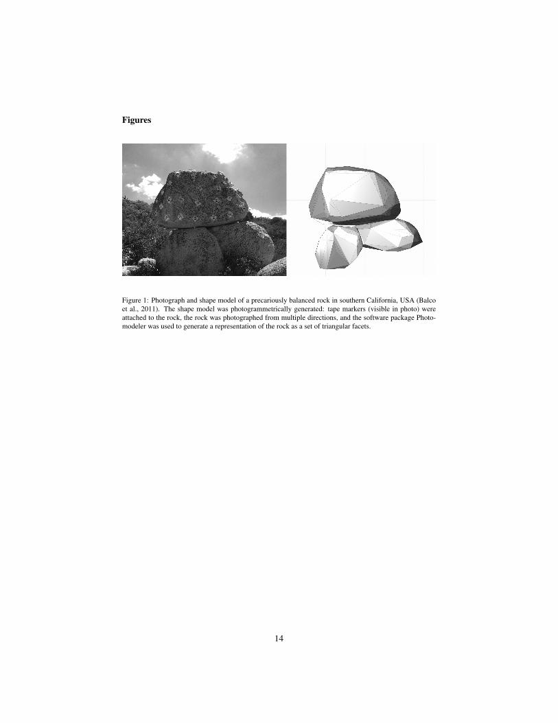
The computer code described in this paper was originally developed for exposure-dating of precariously balanced rocks used in seismic hazard estimation. These rocksare 1-2 meters in size and irregular in shape (e.g., Figure 1), so most sample locationsare partially shielded by the rocks themselves. To quantify these effects, in Balcoet al. (2011) we developed computer code to calculate geometric shielding factors forarbitrarily shaped objects. However, that paper did not include the code or describe itin detail. The present paper provides a complete description and includes the code assupplementary information. In addition, the code and accompanying documentationare available online at http://hess.ess.washington.edu/shielding.

2. Definition of geometric shielding; previous work

The treatment of geometric shielding in this paper follows that of Lal (1991), whichwas also adopted by Dunne et al. (1999), Lal and Chen (2005), and Mackey and Lamb(2013). Dunne et al. (1999) provide a complete and clear derivation of the followingequations. Cosmic ray intensity as a function of direction I(θ, φ), where θ is the zenithangle measured down from the vertical and φ is the azimuthal angle, is assumed to beconstant in azimuth but vary with zenith angle, such that:

I(θ, φ) = I0 cosm (θ) (1)I0 is the maximum intensity (in the vertical direction) and the value of m has been

estimated from cosmic-ray observations and is generally taken to be 2.3 (see Gosse and

3

Phillips, 2001, for additional discussion). The total flux Fre f that an object receives inthe reference case of full exposure to the entire upper hemisphere, that is, when asample site is located on an infinite, unshielded, flat surface, is:

Fre f = I0

∫ 2π

φ=0

∫ π/2

θ=0cosm (θ) sin (θ)dθdφ (2)

This can be evaluated analytically with the result that:

Fre f = I02π

m + 1(3)

Intensity I would typically have units of particles cm−2 sr−1 s−1. However, thepurpose of this work is to calculate a dimensionless shielding factor that is the ratio ofthe production rate at a shielded site to that at an identically located unshielded site, soneither the units nor the absolute value of I or Fre f are relevant.

Geometric shielding is here defined to be the integrated shielding effect of any ob-jects more dense than air that cosmic rays must traverse to reach a sample site. Thisdepends on the size and location of nearby objects relative to the sample. Geometricshielding of the cosmic-ray flux from a particular direction, incident on a particularsample location, can be represented as the mass thickness traversed by cosmic raysfrom that direction before they reach the sample. This mass thickness is ρr(x, y, z, θ, φ)and has units of g cm−2. ρ is the mean density of the material traversed by the cosmicrays (g cm−3). r(x, y, z, θ, φ) is the linear thickness (cm) of this material that a cosmicray arriving from zenith angle θ and azimuth φ must traverse to reach a sample sitewhose location is defined by Cartesian coordinates x, y, and z. Attenuation of cosmicrays traveling in a particular direction is then defined to be exponential in mass thick-ness with a constant attenuation length Λp, such that if the intensity of the incomingcosmic-ray flux in that direction is I0 and the intensity of the cosmic ray flux in thatdirection at the sample site is I, then I/I0 = exp(−ρr/Λp). Note that Λp, which rep-resents an attenuation length along a single incidence direction for cosmic rays withenergies appropriate for inducing spallation reactions in rock, differs from the appar-ent attenuation length for total spallogenic cosmic-ray production with depth below aninfinite flat surface, which is commonly used in exposure-dating calculations and isusually denoted as Λ. Dunne et al. (1999) showed that for constant Λp and m = 2.3,Λp ' 1.3 Λ.

Thus, the cosmic-ray flux at a sample location (x, y, z) subject to geometric shield-ing is:

F = I0

∫ 2π

φ=0

∫ π/2

θ=0cosm (θ) sin (θ)e−

ρr(x,y,z,θ,φ)Λp dθdφ (4)

The dimensionless shielding factor for that sample location relative to an unshieldedsample is then F/Fre f . Computing this requires evaluating the integral in Equation 4,which in turn requires computing the attenuation path length r(x, y, z, θ, φ) for arbitrarysample location and cosmic ray incidence direction.

This approach to computing geometric shielding is routinely used in nuclear physicsto compute fluxes of particles that are simply absorbed in exponential proportion to

4

mass traversed, for example in calculating x- or gamma-ray penetration in objects. Asdiscussed above, however, when applied to calculate shielding factors for high-energycosmic-ray spallation, it disregards the fact that cosmic ray interactions within rockmay yield secondary particles that themselves could contribute to nuclide production.In addition, the assumption of constant Λp is an important simplification. In reality, theattenuation length for cosmic rays depends on their energy. The energy spectrum ofcosmic rays varies with location in the Earth’s atmosphere and magnetic field as wellas with zenith angle, so Λp is also expected to be a function of these parameters. Inaddition, different nuclides of interest are produced by reactions with different thresh-old energies, so a single value of Λp is not expected to be appropriate for all nuclides.Although in this code we have disregarded these effects by assuming constant Λp, iftheoretical predictions of neutron energy spectra, their variation with zenith angle, andthe corresponding variations in effective attenuation length were available for a givensample location (presumably from a first-principles particle physics simulation), thecode could easily be modified to include variable Λp, or to integrate over an energyspectrum in addition to solid angle (the MATLAB code is commented to this effect inthe appropriate locations).

This code is not appropriate for describing attenuation of the cosmic-ray muon flux.However, the effective attenuation length for muons in rock is an order of magnitudeor more longer than that for high-energy neutrons, so the effect of meter-scale surfaceobstructions on production rates due to muons is expected to be negligible.

Several previous authors have computed shielding factors using the assumptionsand formulae described above for regular geometries where attenuation path lengthsr can be represented by analytical functions of x, y, z, φ, and θ. Dunne et al. (1999)computed shielding factors at and below flat and dipping surfaces subject to completeobstruction of the cosmic-ray flux from some fraction of the upper hemisphere. Lal andChen (2005) also computed shielding factors below dipping surfaces, and in additionfor the interior of spherical and cubic boulders. Mackey and Lamb (2013) consideredspheres. However, natural rock landforms that one might wish to exposure date arecommonly irregularly shaped, which requires a numerical integration method. Themethod described here uses Monte Carlo integration to evaluate the integral and a ray-tracing method, applied to a representation of the shielding objects as a set of triangularfacets, to compute the path lengths. This approach is similar to that used by Plug et al.(2007) to compute the cosmic-ray shielding effect of a forest.

3. Description of computer code

The computer code described in this paper is written in MATLAB, a high-levelprogramming language designed for mathematical computation and commonly used byEarth scientists. Several other computational tools for cosmogenic-nuclide productionrate calculations are also written in MATLAB (Balco et al., 2008; Goehring et al.,2010). The typical workflow for using this code would be as follows: First, generatea shape model for the objects of interest. Typically one would use a photogrammetricmethod or a laser scanning system to do this. Second, locate sample locations in thesame coordinate system as the shape model. Finally, use the code supplied here toestimate geometric shielding at the sample site by Monte Carlo integration.

5

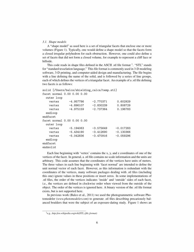
3.1. Shape modelsA “shape model” as used here is a set of triangular facets that enclose one or more

volumes (Figure 1). Typically, one would define a shape model so that the facets forma closed irregular polyhedron for each obstruction. However, one could also define aset of facets that did not form a closed volume, for example to represent a cliff face orhillside.

This code reads in shape files defined in the ASCII .stl file format 1. “STL” standsfor “standard tesselation language.” This file format is commonly used in 3-D modelingsoftware, 3-D printing, and computer-aided design and manufacturing. The file beginswith a line defining the name of the solid, and is followed by a series of line groups,each of which defines the vertices of a triangular facet. An example of a .stl file definingtwo facets is as follows:

solid [/Users/balcs/shielding_calcs/temp.stl]

facet normal 0.00 0.00 0.00

outer loop

vertex -4.957786 -2.770371 0.602929

vertex -4.896107 -2.830239 0.808729

vertex -4.975159 -2.737364 0.196783

endloop

endfacet

facet normal 0.00 0.00 0.00

outer loop

vertex -5.194063 -3.575649 -0.017283

vertex -5.434190 -3.412690 -0.130366

vertex -5.042836 -3.470916 -0.059296

endloop

endfacet

endsolid

Each line beginning with ‘vertex’ contains the x, y, and z coordinates of one of thevertices of the facet. In general, a .stl file contains no scale information and the units arearbitrary. This code assumes that the coordinates of the vertices have units of meters.The three values in each line beginning with ‘facet normal’ are intended to define theunit normal vector of each facet. However, as this information is redundant with thecoordinates of the vertices, many software packages dealing with .stl files (includingthis one) ignore values in these positions or insert zeros. In some implementations of.stl files, the order of the vertices indicates ‘inside’ and ‘outside’ sides of each facet,i.e., the vertices are defined in clockwise order when viewed from the outside of theobject. The order of the vertices is ignored here. A binary version of the .stl file formatexists, but is not supported here.

In previous work (Balco et al., 2011) we used the photogrammetric software Pho-tomodeler (www.photomodeler.com) to generate .stl files describing precariously bal-anced boulders that were the subject of an exposure-dating study. Figure 1 shows an

1e.g., http://en.wikipedia.org/wiki/STL (file format)

6

example. Many commercial and open-source software packages with similar capabili-ties exist.

3.2. Path length calculationA shape model is a collection of sets of three [x, y, z] triples, each set defining a

facet. Given this information and the coordinates of a sample location in the same co-ordinate system, the thickness of rock traversed by a cosmic ray with arbitrary directionis calculated using the following algorithm.

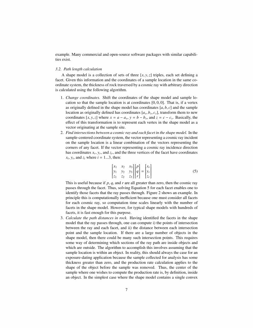
1. Change coordinates. Shift the coordinates of the shape model and sample lo-cation so that the sample location is at coordinates [0, 0, 0]. That is, if a vertexas originally defined in the shape model has coordinates [a, b, c] and the samplelocation as originally defined has coordinates [as, bs, cs], transform them to newcoordinates [x, y, z] where x = a − as, y = b − bs, and z = c − cs. Basically, theeffect of this transformation is to represent each vertex in the shape model as avector originating at the sample site.

2. Find intersections between a cosmic ray and each facet in the shape model. In thesample-centered coordinate system, the vector representing a cosmic ray incidenton the sample location is a linear combination of the vectors representing thecorners of any facet. If the vector representing a cosmic ray incidence directionhas coordinates xr, yr, and zr, and the three vertices of the facet have coordinatesxi, yi, and zi where i = 1...3, then:x1 x2 x3

y1 y2 y3z1 z2 z3

pqr

=

xr

yr

zr

(5)

This is useful because if p, q, and r are all greater than zero, then the cosmic raypasses through the facet. Thus, solving Equation 5 for each facet enables one toidentify those facets that the ray passes through. Figure 2 shows an example. Inprinciple this is computationally inefficient because one must consider all facetsfor each cosmic ray, so computation time scales linearly with the number offacets in the shape model. However, for typical shape models with hundreds offacets, it is fast enough for this purpose.

3. Calculate the path distances in rock. Having identified the facets in the shapemodel that the ray passes through, one can compute i) the points of intersectionbetween the ray and each facet, and ii) the distance between each intersectionpoint and the sample location. If there are a large number of objects in theshape model, then there could be many such intersection points. This requiressome way of determining which sections of the ray path are inside objects andwhich are outside. The algorithm to accomplish this involves assuming that thesample location is within an object. In reality, this should always the case for anexposure-dating application because the sample collected for analysis has somethickness greater than zero, and the production rate calculation applies to theshape of the object before the sample was removed. Thus, the center of thesample where one wishes to compute the production rate is, by definition, insidean object. In the simplest case where the shape model contains a single convex

7

object, then any cosmic ray can only intersect one facet, where it enters the objecton its way to the sample location. In a more complicated case including a singlenon-convex object or many objects, then the ray can enter or exit many differentobjects, or the same object multiple times, intersecting 2n + 1 facets where nis the number of additional objects intersected (or the number of crossings ofone complex object). Thus, one can determine which sections of the ray pathlie within rock by sorting the intersection points according to distance from thesample location and assuming that the pathlength between the sample and theclosest intersection is rock, the pathlength between the closest and second-closestintersections is air, the pathlength between the second-closest and third-closestintersections is rock, and so on. See Figure 2. Note that this algorithm assumesthat all objects are closed shapes, which implies that there will always be anodd number of intersections. An even number of intersections could only arisefrom a topological error in defining the objects in the shape model. However,in practice it might be potentially useful to define some non-closed shapes in ashape model to represent objects that are large enough to fully stop the cosmic-ray flux, e.g., cliff faces or hillsides. To accommodate this, the code provides anoption to assume that an even number of intersections signals total attenuationof a particular cosmic ray.

In applying this method to exposure dating of precariously balanced rocks in Balcoet al. (2011), we also allowed for the possibility that objects were embedded in soilwhose surface lay above the sample site. This can be accounted for by computingthe intersection between the cosmic ray and a horizontal soil surface, disregarding allcosmic ray-facet intersections that lie below the soil surface, and applying the algo-rithm in (3) above to the intersection with the soil surface and any remaining ray-facetintersections.

3.3. Monte Carlo integration

The algorithm described above applied to a shape model enables one to computer(x, y, z, θ, φ). This permits numerical integration of Equation 4 by Monte Carlo inte-gration. Monte Carlo integration is a method of estimating the integral of a functionover some region by generating a uniformly distributed random sample of points withinthe region and computing the value of the function at those points. In general, given afunction of two variables x and y to be integrated over a region 0 ≤ x ≤ a and 0 ≤ y ≤ b,

IMC =abN

N∑i=1

f (xi, yi) '∫ b

0

∫ a

0f (x, y) dx dy (6)

where IMC is the Monte Carlo estimate of the integral, N is the number of pointsin the sample, and the sample points are uniformly distributed in x and y and havecoordinates (xi, yi). Thus, the Monte Carlo estimate for the geometric shielding factorF/Fre f for a sample with coordinates (x, y, z) is:(

2πm + 1

)−1π2

N

N∑i=1

cosm (θi) sin (θi)e−ρr(x,y,z,θi ,φi )

Λp (7)

8

for N sample points (θi, φi) that are uniformly distributed in φ and θ.The number of sample points needed for an accurate Monte Carlo estimate of the

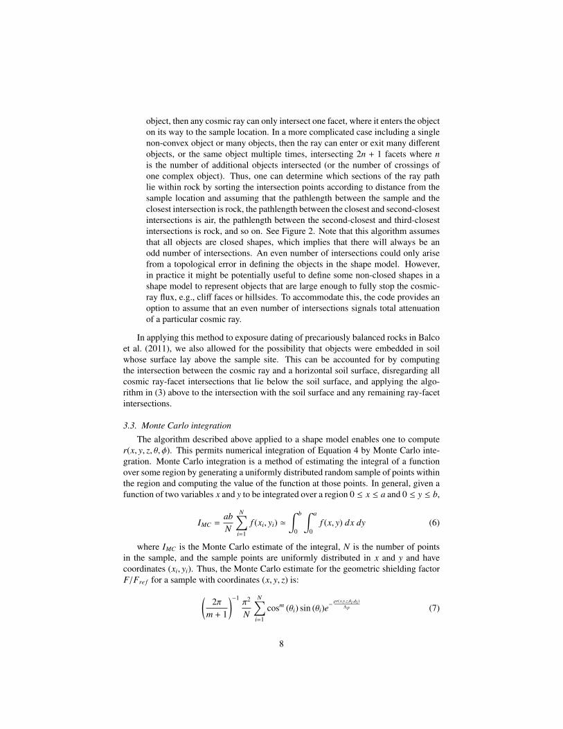
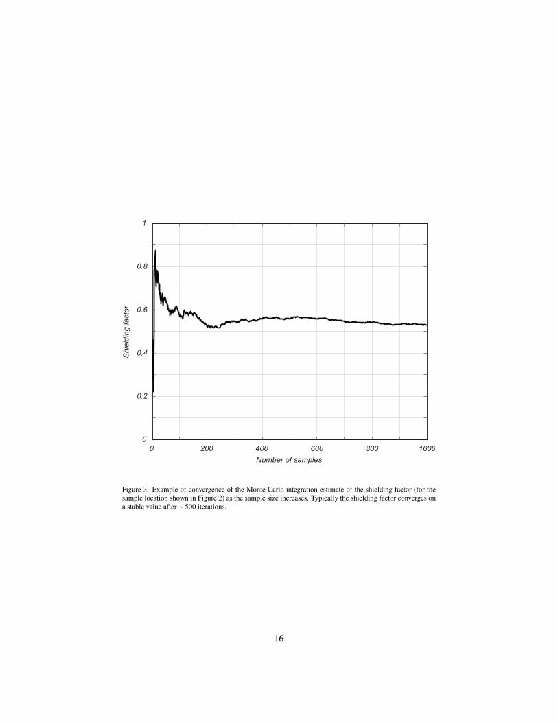
geometric shielding factor depends on the geometry. There exist formal methods ofestimating the uncertainty in a Monte Carlo integral based on the convergence of theresults, but they are not included in the present code. Note that because this calculationincludes systematic uncertainties that stem from the simplifying assumptions discussedabove, the formal uncertainty of the Monte Carlo estimate is not expected to accuratelyrepresent the true uncertainty in the shielding factor. One can informally estimatethe required sample size by successively increasing the number of sample points anddetermining when the resulting shielding factor converges on a stable and reproduciblevalue. Figure 3 shows an example. In the application to precariously balanced rocks,we found that N ' 500 was nearly always sufficient.

3.4. Validation against analytical results

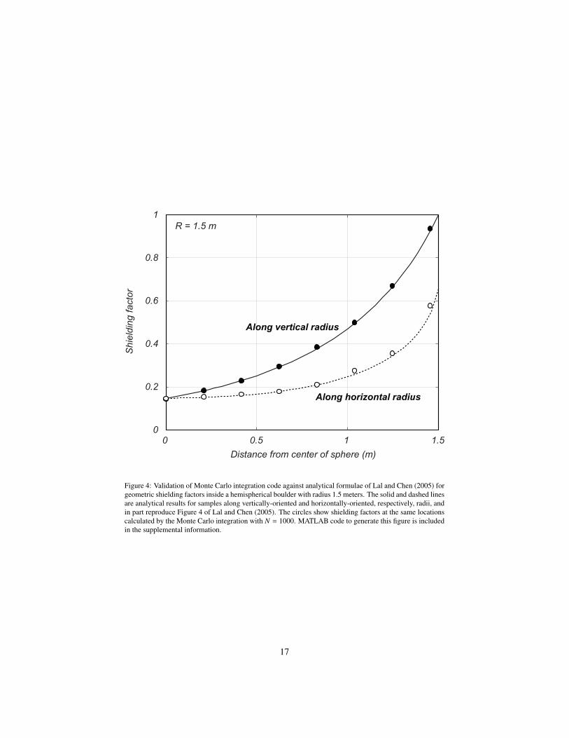
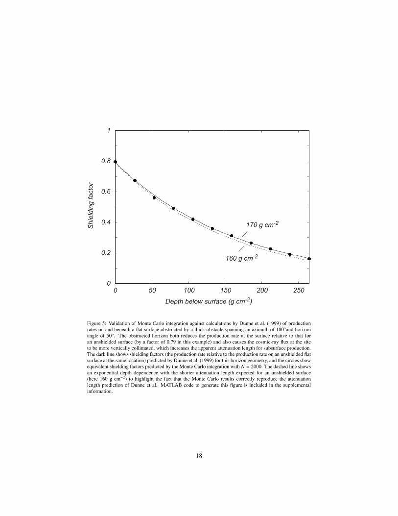
I attempted to validate this code by comparing it to analytical formulae, computedby other authors, for the integral in Equation 4 applied to simple geometries. First,Lal and Chen (2005) derived formulae for computing the geometric shielding factorat points within spherical boulders. In this situation, the cosmic-ray flux is partiallyattenuated by passing through the boulder itself. Figure 4 shows that the Monte Carlointegration yields the same results as their formulae. Second, Dunne et al. (1999)derived formulae for computing shielding due to complete obstruction of portions ofthe upper hemisphere. This case differs from the ones considered by Lal and Chen(2005) and Balco et al. (2011) because it does not involve partial attenuation of thecosmic-ray flux from certain directions, only total obstruction. However, the resultsof Dunne and others are a useful test of this code because they describe not only ashielding factor at the surface due to an obstructed horizon, but also the effect thatthe cosmic-ray flux is more vertically collimated when the horizon is obstructed thanwhen it is not, so the depth-dependence of the production rate varies between thesecases. The Monte Carlo integration can be used to simulate this effect, and Figure 5shows that it correctly reproduces the Dunne et al. results.

3.5. Validation against measurements

In principle, one could validate shielding factors estimated with this code by com-paring them to measured cosmogenic-nuclide concentrations in natural samples. Thiswould require i) an irregularly shaped object with meter-scale dimensions that wasemplaced with zero concentration of cosmic-ray-produced nuclides and subsequentlyexposed to the cosmic-ray flux without any change in its geometry, ii) a shape modelof the object, and iii) measurements of nuclide concentrations from multiple loca-tions on that object that have different degrees of geometric shielding. In this case thecosmogenic-nuclide concentrations will be directly proportional to the true shieldingfactors, allowing straightforward validation of shielding factor estimates. These con-ditions could be satisfied, for example, by sampling several locations on and/or withina glacially transported moraine boulder. However, because nearly all exposure-datingstudies seek to avoid complicated geometric shielding calculations by sampling onlyfrom the top of boulders or outcrops, I am not aware of any such data set.

9

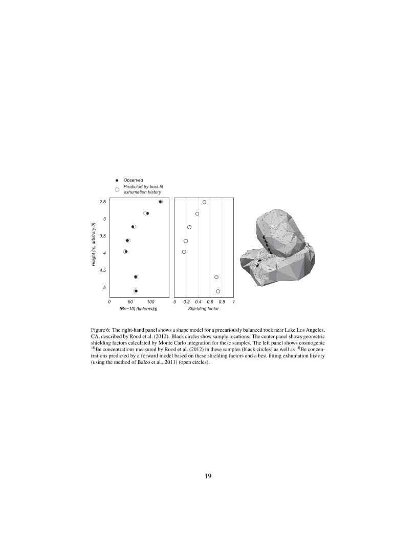
Studies of precariously balanced rocks in Balco et al. (2011) and other more re-cent research (e.g., Rood et al., 2012) collected data that meets some, but not all, ofthese requirements. These data include photogrammetric shape models of irregularlyshaped rocks with meter-scale dimensions, and multiple 10Be measurements at differ-ent locations on these rocks. However, it is not straightforward to use these data toevaluate the accuracy of shielding factor calculations because the rocks were exhumedby downwasting of regolith (and the exhumation history is not known independentlyof the 10Be measurements), so all the samples did not have the same exposure history,and the shielding geometry changed through time. However, these studies were able toclosely match measured 10Be concentrations with a model for 10Be production duringrock exhumation that was based on shielding factors computed using the Monte Carlointegration code described here. Figure 6 shows an example from Rood et al. (2012).Calculated shielding factors for samples from this rock vary by a factor of four (from0.2 to 0.8), and, as shown in Figure 6, variations in measured 10Be concentrations havesimilar pattern and magnitude. Thus, an exhumation history could be found (using themethod of Balco et al., 2011) that was consistent with geomorphic constraints, 10Beconcentrations, and shielding factor estimates.. Because the forward model includesadditional assumptions besides the shielding factor estimates, this comparison does notdirectly validate the shielding factor estimates. However, given the large variation inshielding factor among these samples, it would be difficult to match measured nuclideconcentrations if the shielding factor estimates were highly inaccurate. Again, a betterapproach to this would be to make similar measurements on a boulder with a simpleexposure history. This would be a valuable future contribution.

4. Example uses

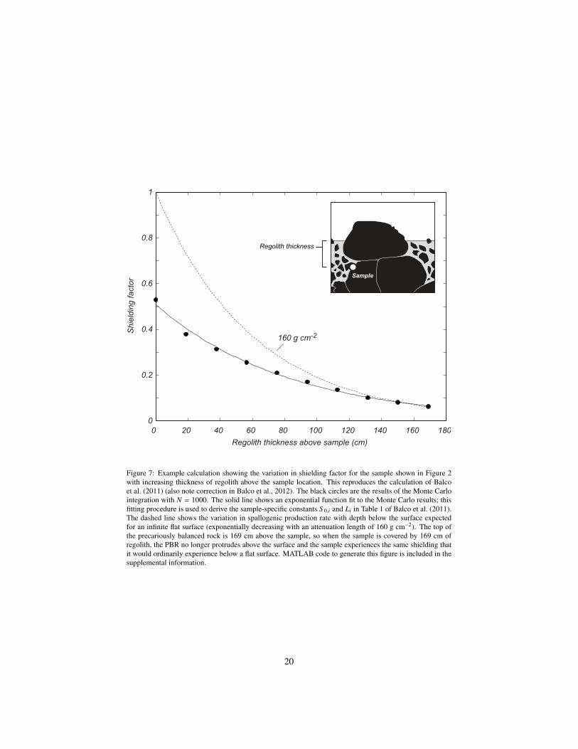
The general purpose of the Monte Carlo integration code is to permit exposure-dating of samples that are surrounded by meter-scale surface obstructions. In manycommon exposure-dating situations, for example exposure-dating of glacially trans-ported boulders, complex shielding calculations of this sort are, of course, mostly notnecessary because it is easier to select unshielded sample sites. The reason this codewas developed for reconstructing exhumation histories of precariously balanced rocksuseful in seismic hazard analysis is because sampling only unshielded parts of thesefeatures did not provide enough information to determine when they were formed. Thefact that the shielding geometry changes as the rocks are exhumed required a relativelysimple and quick method of estimating not only present geometric shielding factors butalso changes in the shielding factor over time. Figure 7 shows an example calculationfor this application, and MATLAB code to generate these results is included in thesupplemental material.

Other obvious applications include estimating erosion rates where soil erosion leadsto progressive exposure of rock features such as tors (e.g., Heimsath et al., 2000), orto estimate when features like arches or sea stacks were formed by cliff retreat. Morecomplex applications would include attempting to determine the frequency of boul-der transport by comparing measured cosmogenic-nuclide concentrations to presentshielding geometries (Mackey and Lamb, 2013); or, potentially, archeological applica-

10

tions aimed at verifying that sculpture or stonework has resided in its present geometricconfiguration since constructed.

5. Acknowledgements.

Dylan Rood provided the impetus for this work by telling me about precariouslybalanced rocks in the first place. This work was supported in part by the Ann andGordon Getty Foundation.

11

Balco, G., Purvance, M., Rood, D., 2011. Exposure dating of precariously balancedrocks. Quaternary Geochronology 6, 295–303.

Balco, G., Purvance, M., Rood, D., 2012. Corrigendum to “Exposure dating of precar-iously balanced rocks” [Quaternary Geochronology 6(2011) 295-303]. QuaternaryGeochronology 9, 86.

Balco, G., Schaefer, J., 2006. Cosmogenic-nuclide and varve chronologies for thedeglaciation of southern New England. Quaternary Geochronology 1, 15–28.

Balco, G., Stone, J., Lifton, N., Dunai, T., 2008. A complete and easily accessiblemeans of calculating surface exposure ages or erosion rates from 10Be and 26Al mea-surements. Quaternary Geochronology 3, 174–195.

Dunai, T., 2010. Cosmogenic Nuclides: Principles, Concepts, and Applications in theEarth Surface Sciences. Cambridge University Press: Cambridge, UK.

Dunne, J., Elmore, D., Muzikar, P., 1999. Scaling factors for the rates of productionof cosmogenic nuclides for geometric shielding and attenuation at depth on slopedsurfaces. Geomorphology 27, 3–12.

Goehring, B., Kurz, M., Balco, G., Schaefer, J., Licciardi, J., Lifton, N., 2010. A reeval-uation of in-situ cosmogenic He-3 production rates. Quaternary Geochronology 5,410–418.

Gosse, J. C., Phillips, F. M., 2001. Terrestrial in situ cosmogenic nuclides: theory andapplication. Quaternary Science Reviews 20, 1475–1560.

Heimsath, A., Chappell, J., Dietrich, W., Nishiizumi, K., Finkel, R., 2000. Soil produc-tion on a retreating escarpment in southeastern Australia. Geology 28 (9), 787–790.

Kubik, P., Reuther, A., 2007. Attenuation of cosmogenic 10Be production in the first20 cm below a rock surface. Nuclear Instruments and Methods in Physics ResearchB 259, 616–624.

Lal, D., 1991. Cosmic ray labeling of erosion surfaces: in situ nuclide production ratesand erosion models. Earth Planet. Sci. Lett. 104, 424–439.

Lal, D., Chen, J., 2005. Cosmic ray labeling of erosion surfaces II: Special cases ofexposure histories of boulders, soil, and beach terraces. Earth and Planetary ScienceLetters 236, 797–813.

Mackey, B., Lamb, M., 2013. Deciphering boulder mobility and erosion from cosmo-genic nuclide exposure dating. Journal of Geophysical Research - Earth Surface 118,184–197.

Masarik, J., Beer, J., 1999. Simulation of particle fluxes and cosmogenic nuclide pro-duction in Earth’s atmosphere. Journal of Geophysical Research 104, 12099–12111.

Masarik, J., Wieler, R., 2003. Production rates of cosmogenic nuclides in boulders.Earth and Planetary Science Letters 216, 201–208.

12

Plug, L., Gosse, J., McIntosh, J., Bigley, R., 2007. Attenuation of cosmic ray flux intemperate forest. Journal of Geophysical Research 112, F02022.

Rood, D., Anooshehpoor, R., Balco, G., Biasi, G., Brune, J., Brune, R., Grant Ludwig,L., Kendrick, K., Purvance, M., Saleeby, I., 2012. Testing seismic hazard modelswith be-10 exposure ages for precariously balanced rocks. American GeophysicalUnion 2012 Fall Meeting, San Francisco, CA. Abstract 1493571.

13

Figures

Figure 1: Photograph and shape model of a precariously balanced rock in southern California, USA (Balcoet al., 2011). The shape model was photogrammetrically generated: tape markers (visible in photo) wereattached to the rock, the rock was photographed from multiple directions, and the software package Photo-modeler was used to generate a representation of the rock as a set of triangular facets.

14

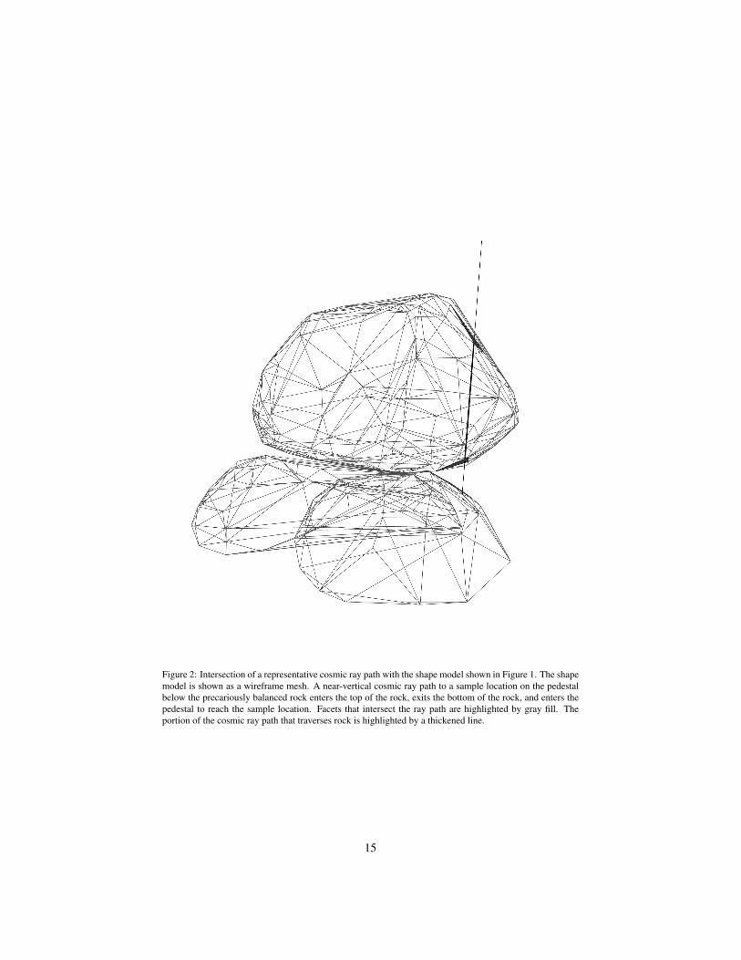
Figure 2: Intersection of a representative cosmic ray path with the shape model shown in Figure 1. The shapemodel is shown as a wireframe mesh. A near-vertical cosmic ray path to a sample location on the pedestalbelow the precariously balanced rock enters the top of the rock, exits the bottom of the rock, and enters thepedestal to reach the sample location. Facets that intersect the ray path are highlighted by gray fill. Theportion of the cosmic ray path that traverses rock is highlighted by a thickened line.

15

0 200 400 600 800 1000

0

0.2

0.4

0.6

0.8

1

Number of samples

Sh

ield

ing

fa

cto

r

Figure 3: Example of convergence of the Monte Carlo integration estimate of the shielding factor (for thesample location shown in Figure 2) as the sample size increases. Typically the shielding factor converges ona stable value after ∼ 500 iterations.

16

0 0.5 1 1.50

0.2

0.4

0.6

0.8

1

R = 1.5 m

Distance from center of sphere (m)

Sh

ield

ing

fa

cto

r

Along vertical radius

Along horizontal radius

Figure 4: Validation of Monte Carlo integration code against analytical formulae of Lal and Chen (2005) forgeometric shielding factors inside a hemispherical boulder with radius 1.5 meters. The solid and dashed linesare analytical results for samples along vertically-oriented and horizontally-oriented, respectively, radii, andin part reproduce Figure 4 of Lal and Chen (2005). The circles show shielding factors at the same locationscalculated by the Monte Carlo integration with N = 1000. MATLAB code to generate this figure is includedin the supplemental information.

17

0 50 100 150 200 2500

0.2

0.4

0.6

0.8

1

Sh

ield

ing

fa

cto

r

Depth below surface (g cm-2)

160 g cm-2

170 g cm-2

Figure 5: Validation of Monte Carlo integration against calculations by Dunne et al. (1999) of productionrates on and beneath a flat surface obstructed by a thick obstacle spanning an azimuth of 180°and horizonangle of 50°. The obstructed horizon both reduces the production rate at the surface relative to that foran unshielded surface (by a factor of 0.79 in this example) and also causes the cosmic-ray flux at the siteto be more vertically collimated, which increases the apparent attenuation length for subsurface production.The dark line shows shielding factors (the production rate relative to the production rate on an unshielded flatsurface at the same location) predicted by Dunne et al. (1999) for this horizon geometry, and the circles showequivalent shielding factors predicted by the Monte Carlo integration with N = 2000. The dashed line showsan exponential depth dependence with the shorter attenuation length expected for an unshielded surface(here 160 g cm−2) to highlight the fact that the Monte Carlo results correctly reproduce the attenuationlength prediction of Dunne et al. MATLAB code to generate this figure is included in the supplementalinformation.

18

0 50 100

[Be−10] (katoms/g)

2.5

3

3.5

4

4.5

5

He

igh

t (m

, a

rbitra

ry 0

)

Observed

Predicted by best-fit

exhumation history

0 0.80.60.40.2 1

Shielding factor

Figure 6: The right-hand panel shows a shape model for a precariously balanced rock near Lake Los Angeles,CA, described by Rood et al. (2012). Black circles show sample locations. The center panel shows geometricshielding factors calculated by Monte Carlo integration for these samples. The left panel shows cosmogenic10Be concentrations measured by Rood et al. (2012) in these samples (black circles) as well as 10Be concen-trations predicted by a forward model based on these shielding factors and a best-fitting exhumation history(using the method of Balco et al., 2011) (open circles).

19

0 20 40 60 80 100 120 140 160 180

0

0.2

0.4

0.6

0.8

1

Regolith thickness above sample (cm)

Sh

ield

ing

fa

cto

r

160 g cm-2

Sample

Regolith thickness

Figure 7: Example calculation showing the variation in shielding factor for the sample shown in Figure 2with increasing thickness of regolith above the sample location. This reproduces the calculation of Balcoet al. (2011) (also note correction in Balco et al., 2012). The black circles are the results of the Monte Carlointegration with N = 1000. The solid line shows an exponential function fit to the Monte Carlo results; thisfitting procedure is used to derive the sample-specific constants S 0,i and Li in Table 1 of Balco et al. (2011).The dashed line shows the variation in spallogenic production rate with depth below the surface expectedfor an infinite flat surface (exponentially decreasing with an attenuation length of 160 g cm−2). The top ofthe precariously balanced rock is 169 cm above the sample, so when the sample is covered by 169 cm ofregolith, the PBR no longer protrudes above the surface and the sample experiences the same shielding thatit would ordinarily experience below a flat surface. MATLAB code to generate this figure is included in thesupplemental information.

20