C H A P T E R 7 S I T E D I S P L A C E M E N T

Local Si te D i s p l a c e m e n t due t o Ocean Loading

Local site displacement is understood as an effect of (visco-) elastic deformation of the Earth in response to time-varying surface loads. The reference point of zero deformation is the Joint mass center of the solid Earth and the load, while the sites are attached to the solid Ear th . This Convention implies that the rigid body translation of the solid Earth that counterbalances the motion of the load's mass center is not contained in the local displacement model. This Convention follows strictly Farrell (1972).

Ocean Loading

Three dimensional site displacements due to ocean tide loading are computed using the following scheme. Let Ac denote a displacement component (radial, west, south) at a particular site and time t. Let W denote the tide generating potential (e.g. Tamura, 1987; Cartwright and Tayler, 1971; Cartwright and Edden, 1973),

W = g ^2 ^3PTi ( c o s ^ ) ^os(ujt + Xj + mjX), (1) i

where only degree two harmonics are retained. The Symbols designate colatitude ip, longitude A, tidal angular velocity Uj, amplitude Kj and the astronomical argument \j at t = 0h. Spherical harmonic order mj distinguishes the fundamental bands, i. e. long-period (m = 0), diurnal (m = 1) and semi-diurnal (ra = 2). The parameters Kj and Uj are used to obtain the most completely interpolated form

A c = ] C a°j cm^u;ii + Xi - <l>cj h (2) j

with \Ackcos$ck A e ,M - 1cos$ c ? f c+ 1 1

acj cos<j>cj = hj\ r. (1 - p) + jz p\, L &k Afc+l J

. \Ack$m$ck A c , f c + i s in$ c , f c + 1 acj sin (ßcj = hj\ y (1 - p) + — l - r ! P

/̂c+l

For each site, the amplitudes Ack and phases $CA:,1 < k < 11, are taken from Table 7.1. For clarity symbols written with bars overhead designate tidal potential quantities associated with the small set of partial tides represented in the table. These are the semi-diurnal waves M 2 , 5 2 , A^2,Ä'2? the diurnal waves K\,0\,P\,Q\, and the long-period waves Mj,Mm, and Ssa.

Interpolation is possible only within a fundamental band, i.e. we demand

mfc = m j = räfc+i. (3)

Then &j — U>fc

P = -= —, Uk < Uj < Lük+i. <*>*+l - Uk

If no ük or ük+\ can be found meeting (3), p is set to zero or one, respectively.

52

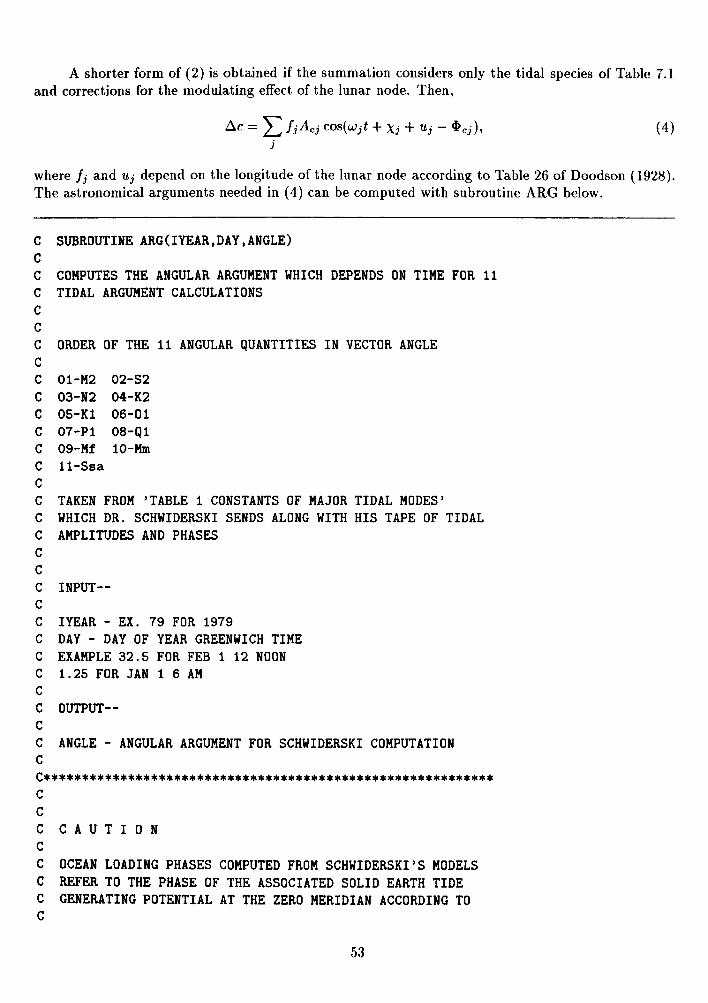
A shorter form of (2) is obtained if the summation considers only the tidal species of Table 7.1 and corrections for the modulating effect of the lunar node. Then,

Ac = J2 fjAcj cos(ujjt + Xj + Uj- $ c j ) , (4) j

where fj and Uj depend on the longitude of the lunar node according to Table 26 of Doodson (1928). The astronomical arguments needed in (4) can be computed with subroutine ARG below.

C SUBROUTINE ARG(IYEAR,DAY,ANGLE) C C COMPUTES THE ANGULAR ARGUMENT WHICH DEPENDS ON TIME FOR 11 C TIDAL ARGUMENT CALCULATIONS

C C C ORDER OF THE 11 ANGULAR qUANTITIES IN VECTOR ANGLE

C C 01-M2 02-S2 C 03-N2 04-K2 C 05-K1 06-01 C 07-P1 08-Q1 C 09-Mf 10-Mm C 11-Ssa C C TAKEN FROM 'TABLE 1 CONSTANTS OF MAJOR TIDAL MODES' C WHICH DR. SCHWIDERSKI SENDS ALONG WITH HIS TAPE OF TIDAL C AMPLITUDES AND PHASES

C C

C INPUT— C C IYEAR - EX. 79 FOR 1979 C DAY - DAY OF YEAR GREENWICH TIME

C EXAMPLE 32.5 FOR FEB 1 12 NOON C 1.25 FOR JAN 1 6 AM C C OUTPUT— C

C ANGLE - ANGULAR ARGUMENT FOR SCHWIDERSKI COMPUTATION C C***********************************************************

c

c

C C A U T I O N

C

C OCEAN LOADING PHASES COMPUTED FROM SCHWIDERSKI'S MODELS

C REFER TO THE PHASE OF THE ASSOCIATED SOLID EARTH TIDE C GENERATING POTENTIAL AT THE ZERO MERIDIAN ACCORDING TO C

53

C OLJ)R = OL_AMP X COS (SE_PHASE" - OL-PHASE) C C WHERE OL = OCEAN LOADING TIDE, C SE = SOLID EARTH TIDE GENERATING POTENTIAL.

C C IF THE HARMONIC TIDE DEVELOPMENT OF CARTWRIGHT, ET AL. C ( = CTE) (1971, 1973) IS USED, MAKE SURE THAT SE-PHASE" C TAKES INTO ACCOUNT

C C (1) THE SIGN OF SE_AMP IN THE TABLES OF CARTWRIGHT ET AL. C C (2) THAT CTE'S SE.PHASE REFERS TO A SINE RATHER THAN A C COSINE FUNCTION IF (N+M) = (DEGREE + ORDER) OF THE C TIDE SPHERICAL HARMONIC IS ODD. C

C I.E. SEJPHASE" = TAU(T) NI + S(T) N2 + H(T) N3 C + P(T) N4 + N'(T) N5 + PS(T) N6

C + PI IF CTE'S AMPLITUDE COEFFICIENT < 0 C + PI/2 IF (DEGREE + NI) IS ODD C C WHERE TAU ... PS = ASTRONOMICAL ARGUMENTS, C NI ... N6 - CTE'S ARGUMENT NUMBERS. C

C MOST TIDE GENERATING SOFTWARE COMPUTE SE_PHASE" (FOR

C USE WITH COSINES). C

C THIS SUBROUTINE IS VALID ONLY AFTER 1973. C C******************************************************************

SUBROUTINE ARG(IYEAR,DAY,ANGLE)

IMPLICIT DOUBLE PRECISION (A-H,0-Z) REAL ANGFAC(4,11) DIMENSION ANGLE(11),SPEED(11)

C C SPEED OF ALL TERMS IN RADIANS PER SEC C

EqUIVALENCE (SPEED(l),SIGM2),(SPEED(2),SIGS2),(SPEED(3).SIGN2)

EQUIVALENCE (SPEED(4),SIGK2),(SPEED(5).SIGK1),(SPEED(6).SIGOl) EQUIVALENCE (SPEED(7),SIGP1),(SPEED(8),SIGQ1),(SPEED(9),SIGMF) EqUIVALENCE (SPEED(10),SIGMM),(SPEED(ll).SIGSSA) DATA SIGM2/1.40519D-4/ DATA SIGS2/1.45444D-4/ DATA SIGN2/1.37880D-4/ DATA SIGK2/1.45842D-4/ DATA SIGK1/.72921D-4/ DATA SIGOl/.67598D-4/

DATA SIGP1/.72523D-4/ DATA SIGQ1/.64959D-4/

DATA SIGMF/.053234D-4/

54

DATA SIGMM/.026392D-4/ DATA SIGSSA/.003982D-4/ DATA ANGFAC/2.E0,-2.E0,0.E0,0.E0,4*0.E0, 2.E0,-3.E0,1.E0,0.E0,2.E0,3*0.E0, l.EO,2*O.EO,.25EO,l.E0,-2.EO,O.E0,-.25EO, -i.E0,2*0.E0,-.25E0,l.E0,-3.E0,l.E0,-.25E0, 0.E0,2.E0,2*0.E0,0.E0,1.E0,-1.E0,0.E0, 2.E0,3*0.E0/

DATA TWOPI/6.28318530718DO/ DATA DTR/.174532925199D-1/

C

C DAY OF YEAR C

ID=DAY C C FRACTIONAL PART OF DAY IN SECONDS C

FDAY=(DAY-ID)*86400.DO ICAPD=ID+365*(IYEAR-75)+((IYEAR-73)/4) CAPT*(27392.500528D0+1.000000035D0*ICAPD)/36525.DO

C

C MEAN LONGITUDE OF SUN AT BEGINNING OF DAY C

HO=(279.69668D0+(36000.768930485D0+3.03D-4*CAPT)*CAPT)*DTR C C MEAN LONGITUDE OF MOON AT BEGINNING OF DAY C

S0=(((1.9D-6+CAPT-.001133D0)*CAPT+481267.88314137D0)*CAPT . +270.434358D0)*DTR

C

C MEAN LONGITUDE OF LUNAR PERIGEE AT BEGINNING OF DAY C

P0=(((-1.2D-5*CAPT-.010325D0)*CAPT+4069.0340329577D0)*CAPT . +334.329653D0)*DTR DO 500 K-1,11

ANGLE(K)=SPEED(K)*FDAY+ANGFAC(1,K)*H0+ANGFAC(2,K)*S0 . +ANGFAC(3,K)*PO+ANGFAC(4,K)*TWOPI ANGLE(K)=DMOD(ANGLE(K).TWOPI) IF(ANGLE(K).LT.O.DO)ANGLE(K)=ANGLE(K)+TW0PI

500 CONTINUE RETURN END

Table 7.1 is available electronically by anonymous ftp to m a i a . u s n o . n a v y . m i l or f t p : / / g e r e . o s o . c h a l m e r s . s e / ~ p u b / h g s / o l o a d / R E A D M E . For sites not contained in the list the fol­lowing is recommended: If the distance to the nearest site contained in the table is less than ten km, its da ta can be substituted. In other cases, coefficients and/or Software can be requested from hgsf loso .chalmers . se (Hans-Georg Scherneck). The Tamura tide potential is available from the International Centre for Earth Tides, Observatoire Royal de Belgique, Bruxelles.

55

The coefficients of Table 7.1 have been computed according to Scherneck (1983,1991). Tangential displacements are to be taken positive in west and south directions. The ocean tide maps adopted are due to LeProvost et al. (1994), Schwiderski (1983), Schwiderski and Szeto (1981), and Fiather (1981). Refined coastlines have been derived from the topographic data sets E T 0 P 0 5 and Terrain Base (Row et ai, 1995) of the National Geophysical Data Center, Boulder, CO. Ocean tide mass budgets have been constrained using a uniform co-oscillating oceanic layer. Load convolution employed a disk-integrating Green's function method (Farrell, 1972; Zschau, 1983; Scherneck, 1990). An assessment of the accuracy of the loading model is given in Scherneck (1993). Adoption of more recent ocean tide results drawing from TOPEX/POSEIDON results is currently under consideration.

Table 7.1 Sample of ocean loading table file. Each site record shows a header with the site name, the CDP monument number, geographic coordinates and comments. First three rows of numbers designate amplitudes (meter), radial, west, south, followed by three lines with the corresponding phase values (degrees).

Columns designate partial tides M2,S2,N2, A ' 2 , K \ , 0 \ , P i , Q i , M f , M m , and Ss

$$ 0NSALA6O 7213

$$ $$ Computed by H.G. Scherneck, Uppsala U n i v e r s i t y , 1989 $$ ONSALA 7213

.00384 .00091

.00124

.00058 - 5 6 . 0

7 5 . 4 8 4 . 2

.00034

.00027 - 4 6 . 1

9 7 . 6 131 .3

l o n / l a t : 11.9263 57.3947 .00084 .00019 .00224 .00031 .00009 .00042 .00021 .00008 .00032

- 9 0 . 7 - 3 4 . 4 - 4 4 . 5 4 0 . 8 94 .8 119.0 77 .7 103.9 17 .2

.00120 .

.00041 .

.00017 .

-123.2 25.4 -55.0

.00071

.00015

.00009 -49.6

98.7 25.2

.00003

.00006

.00004 178.4

-14.1 -165.0

.00084

.00018

.00007 14.9

-177.0

173.3

.00063

.00010

.00001 37.3

-126.7 121.8

.00057

.00010

.00020 24.6

-175.8 91.3

Effects of t h e Solid Earth Tides

Site displacements caused by tides of sperical harmonic degree and order (nm) are characterized by the Love number hnm and the Shida number lnm. The effective values of these numbers depend on Station latitude and tidal frequency (Wahr, 1981). This dependence is a consequence of the ellipticity and rotation of the Earth, and includes a strong frequency dependence within the diurnal band due to the Nearly Diurnal Free Wobble resonance. A further frequency dependence, which is most pronounced in the long period tidal band, arises from mantle anelasticity which leads to corrections to the elastic Earth Love numbers; these corrections have a small imaginary part and cause the tidal displacements to lag slightly behind the tide generating potential. All these effects need to be taken into account when an accuracy of 1 mm is desired in determining Station positions.

In order to account for the latitude dependence of the effective Love and Shida numbers, the representation in terms of multiple h and / parameters employed by Mathews et al. (1995) is used. In this representation, parameters h^ and l^ play the roles of /^m and / 2 m , while the latitude dependence is expressed in terms of additional parameters h^2),hf and / ( 1 \ / ( 2 ) , / ' . These parameters are defined through their contributions to the site displacement as given by equations (5) below. Their numerical values as listed in Mathews et al. (1995) have since been revised, and the new values, presented in Table 7.2 are used here. These values pertain to the elastic Earth and anelasticity modeis referred to in Chapter 6.

56

The vector displacement due to a tidal term of frequency / is given in terms of the several parameters by the following expressions that result from evaluation of the defining equation (6) of Mathews et al. (1995):

For a long-period tide of frequency / :

Afj * , { [ « « ( ! * ' • - £ ) + , / £ » ' cos 0ff + 3/(0) sin <fr cos <ß cos 0j h

+ cos0 3 / ( 1 W < £ - * & ' V 5

sin 0j e \

(5a)

For a diurnal tide of frequency / :

Af/ = 24TT

HJ < /i(0)3 sin 0 cos 0 sin(0/ + A) r

+

+

3/(0) cos20 - 3 / ( 1 ) sin2 0 + J^-l' sin(9f + X)h

13/(0) - J^r-l') sin 0 - 3 / ( 1 ) sin 0 c o s 2 0 cos(fy + A)e

(56)

For a semidiurnal tide of frequency / :

A f ; = J — ///{[/?(0)3cos2 0cos (0 , + 2A)f - 6 s in0cos0 [ / (0 ) + / ( 1 ) ]cos(0 , + 2A)n

- 6cos0[ / (0) + / ( 1 ) sin2 0] sin(0/ 4- 2A) e).

(5c)

In the above expressions,

h{4>) = h{0) + /i ( 2 )[(3/2) sin2 0 - 1/2], /(0) = /<°> + / ( 2 )[(3/2) sin2 0 - 1/2],

Hj = amplitude (m) of the tidal term of frequency / ,

0 = geocentric latitude of Station,

A = east longitude of Station,

Oj = tide argument for tidal constituent with frequency / ,

57

(6)

e = unit vector in the east direction,

h = unit vector at right angles to f in the northward direction.

The Convention used in defining the tidal amplitude Hf is as in Cartwright and Tayler (1971). To convert amplitudes defined according to other Conventions tha t have been employed in recent more accurate tables, use the conversion factors given in Chapter 6, Table 6.4.

Equations (5) assume that the Love and Shida number parameters are all real. Generalization to the case of complex parameters (anelastic earth) is done simply by making the following replacements for the combinations Lcos(0j + mX) and Lsin(0f + mX), wherever they occur in those equations:

Lcos(0f + mX) -* LRcos(0f + raA) - L1 sin(0f + mX), (7a)

Lsh\(0f + mX) — LRsm(0f + raA) + L1 cos(0f + mA), (76)

where L is a generic symbol for ft(</>),ft',/(<£),/*x), and / \ and LR and L1 stand for their respective real and imaginary parts . Table 7.2 lists the values of the Love and Shida number parameters. The Earth model on which they are based is the 1 see PREM, modified by replacement of the ocean layer by solid (Dehant, 1987, Wang, 1994) and by adjustment of the fluid core ellipticity to make the FCN period = 430 sidereal days as inferred from the resonance in nutations. The tidal frequencies shown in the table are in cycles per sidereal day (epsd). Periods, in solar days, of the nutations associated with the diurnal tides are also shown.

Table 7.2. Displacement Love number parameters for degree 2 tides. Quantities with subscripts elas (anelas) are computed ignoring (including) anelasticity effects. Superscripts R and I identify the real and imaginary parts , respectively.

Name Period Frequency h.nm hn*lnm Äl * *„. ~ * elas anelas anelas

Semidiurnal -2 epsd .6026 .6078 -.0022

Ä<2>

.0006

Diurnal

Qi 145,545

Oi NOi

Pl 165,545

Ki 165,565

01 01

9.13 13.63 13.66 27.55

121.75 182.62

6798.38 infinity

-6798.38 -365.26 -182.62

-0.89080 -0.92685 -0.92700 -0.96381 -0.99181 -0.99454 -0.99985 -1.00000 -1.00015 -1.00273 -1.00546

.5971

.5964

.5964

.5941

.5813

.5753

.5214

.5166

.5112 1.0582

.6589

.6033

.6026

.6026

.6003

.5876

.5816

.5280

.5232

.5178 1.0534

.6644

-.0025 -.0025 -.0025 -.0025 -.0025 -.0025 -.0027 -.0027 -.0027 .0020 -.0022

.0006

.0006

.0006

.0006

.0007

.0007 -.0007 -.0008 -.0008 -.0001 -.0006

58

Long period 55,565

"sa Mm

Ms

75,565

Name

Semidiurnal

Diurnal

Qi 145,545

Oi Mi

Tl Pl

165,545

Ki 165,565

01 01

Long period

55,565

•-'so Mm

Mj 75,565

6798.38 182.62 27.55

13.66 13.63

.000015

.000546

.003619

.007300

.007315

Period Frequency

9.13

13.63

13.66 27.55

121.75 182.62

6798.38 infinity

-6798.38

-365.26 -182.62

6798.38 182.62

27.55 13.66

13.63

-2 epsd

-0.89080 -0.92685

-0.92700 -0.96381

-0.99181 -0.99454

-0.99985 -1.00000 -1.00015

-1.00273 -1.00546

.000015

.000546

.003619

.007300

.007315

.5998

.5998

.5998

.5998

.5998

.6344 -.0093 -.

.6182 -.0054 -.

.6126 -.0041 -.

.6109 -.0037 -.

.6109 -.0037 -.

,(0) ,(0)ß ,(0)/ elas anelas anelas

.0831

.0829

.0829

.0829

.0830

.0834

.0836

.0853

.0854

.0856

.0684

.0810

.0831

.0831

.0831

.0831

.0831

.0847 -.0007

.0848 -.0007

.0848 -.0007

.0848 -.0007

.0849 -.0007

.0853 -.0007

.0855 -.0007

.0871 -.0007

.0872 -.0007

.0874 -.0007

.0710 -.0010

.0829 -.0008

.0936 -.0028

.0886 -.0016

.0870 -.0012

.0864 -.0011

.0864 -.0011

IM

.0024

.0012

.0012

.0012

.0012

.0012

.0012

.0011

.0011

.0011

.0019

.0013

.0000

.0000

.0000

.0000

.0000

0006 .

0006 . 0006 .

0006 . 0006 .

t(2)

.0002

.0002

.0002

.0002

.0002

.0002

.0002

.0002

.0002

.0002

.0002

.0002

.0002

.0002

.0002

.0002

.0002

0001

0001 0001 0001 0001

/ '

-.0002

-.0002

-.0002 -.0002

-.0002 -.0002

-.0003 -.0003 -.0003

.0001 -.0002

Computation of the variations of Station coordinates due to solid Earth tides, like that of geopo­tential variations, is done most efficiently by the use of a two-step procedure. The evaluations in the first step use the expression in the time domain for the füll degree 2 tidal potential or for the parts that pertain to particular bands (m = 0 , 1 , or 2). Nominal values used for the Love and Shida numbers /*2m and 1.2m are common to all the tidal constituents involved in the potential and to all stations. They are chosen with reference to the values in Table 7.2 so as to minimize the computational effort needed in Step 2. Along with expressions for the dominant contributions from h^ and / ( 0 ) to the tidal displacements, relatively small contributions from some of the other parameters are included in Step 1 for reasons of computational efficiency. The displacements caused by the degree 3 tides are also computed in the first step, using constant values for h$ and 1%.

Corrections to the results of the first step are needed to take account of the frequency dependent deviations of the Love and Shida numbers from their respective nominal values, and also to compute

59

the out of phase contributions from the zonal tides. The scheme of computation is outlined in the chart below.

CORRECTIONS FOR THE STATION TIDAL DISPLACEMENTS

Step 1 : Corrections to be computed in the time domain

in phase for degree 2 and 3 Nominal values . for degree 2 — eq (8) h2 — h(4>) = fc(0) + /i (2 )[(3sin2 <t> - l ) / 2 ]

l2 -+ /(</>) = /(°) + /(2)[(3 sin2 <j> - l ) /2 ] elastic Ä<°> = 0.6026, h^ = -0 .0006; / ( 0 ) = 0.0831, /<2> = 0.0002 anelastic / i ( 0 ) = 0.6078, h{2) = -0 .0006; / ( 0 ) = 0.0847, / ( 2 ) = 0.0002

. for degree 3 - • eq (9) h3 = 0.292 and /3 = 0.015

out-of-phase for degree 2 only Nominal values . diurnal tides — eq (13) hl = -0 .0025 and ll = -0 .0007 . semi-diurnal tides -+ eq (14) h1 = -0.0022 and l1 = -0 .0007

contribution from latitude dependence Nominal values . diurnal tides -* eq (11) /W = 0.0012 . semi-diurnal tides — eq (12) / (1 ) = 0.0024

Step 2 : Corrections to be computed in the frequency domain and to be added to results of Step 1

in phase for degree 2 . diurnal tides —>• eqs (15) —* Sum over all the components of Table 7.3a . semi-diurnal tides negligible

in phase and out of phase for degree 2 . long-period tides —- eqs (16) —• Sum over all the components of Table 7.3b

Displacement due to degree 2 tides, with nominal values for h2m and l2m

The first stage of the S t ep 1 calculations employs real nominal values /12 and /2 common to all the degree 2 tides for the Love and Shida numbers. It is found to be computationally most economical to choose these to be the values for the semidiurnal tides (which have very little intraband Variation). For the same reason, the nominal values used when anelasticity is included are different from the elastic case. (Anelasticity contributions are at the one percent level, which is about 4 rara in the radial displacement due to the füll degree 2 tide.) The out of phase contributions due to anelasticity are dealt with separately below.

On using the nominal values, the vector displacement of the Station due to the degree 2 tides is given by

60

A f = E § ^ { h ^ ( h Ä r f ) 2 - l ) + 3h(RJ-mj-(k-r)f}^ (8)

where h22 and l22 of the semidiurnal tides are chosen as the nominal values h<i and /2 . These values depend on whether anelasticity is included in the computation or not, but no imaginary parts are included at this stage. In equation (8),

GMj = gravitational parameter for the Moon (j = 2) or the Sun (j = 3),

GM® = gravitational parameter for the Earth,

Rj, Rj = unit vector from the geocenter to Moon or Sun and the magnitude of that vector,

Re = Ear th 's equatorial radius,

f,r= unit vector from the geocenter to the Station and the magnitude of that vector,

/i2 = nominal degree 2 Love number,

1-2 = nominal degree 2 Shida number.

Note that the part proportional to /i2 gives the radial (not vertical) component of the tide-induced Station displacement, and the terms in I2 represent the vector displacement transverse to the radial direction (and not in the horizontal plane).

The computation just described may be generalized to include the latitude dependence arising through h^ by simply adding /^2 )[(3/2)sin2 <j) - (1/2)] to the constant nominal value given above, with h{2) = -0 .0006. The addition of a similar term (with / ( 2 ) = 0.0002) to the nominal value of l2

takes care of the corresponding contribution to the transverse displacement. The resulting incremental displacements are small, not exceeding 0.4 rara radially and 0.2 rara in the transverse direction.

Displacements due to degree 3 tides

The Love numbers of the degree 3 tides may be taken as real and constant in computations to the degree of accuracy aimed at here. The vector displacement due to these tides is then given by

^ - t ^ | M i ' * J - ' i , - l < * > - ' ) ) + ' > ( T ( * ' - " , - i ) ' * ' - ( * ' - " 4 , 9 )

Only the Moon's contribution (j = 2) need be computed, the term due to the Sun being quite ignorable. The transverse part of the displacement (9) does not exceed 0.2 rara, but the radial displacement can reach 1.7 rara.

61

Contributions to the transverse displacement due to the l^ term

The imaginary part of l^ (anelastic case) is completely ignorable, and so is the difference between the real part and the elastic Earth value, as well as the intra-band frequency dependence; and l^ is effectively zero in the zonal band.

In the expressions given below, and elsewhere in this Chapter,

$j — body fixed geocentric latitude of Moon or Sun, and

Xj — body fixed east longitude (from Greenwich) of Moon or Sun.

The following formulae may be employed when the use of Cartesian coordinates Xj, Yj, Zj of the body relative to the terrestrial reference frame is preferred:

P 2 °(s in$ j ) = - l Q z 2 - i Ä 2 ) , (10a)

9 V . 7 . QV.7. Pl (sin $,-) cos A, = —±^, P\ (sin * , ) sin A,- = -j^-, (106)

P 22 ( s in# j )cos2A j = ~^(X] - Yj), P 2

2 ( s in$ j ) s in2A j = -^XjYj. (10c)

Contribution from the diurnal band (with l^ = 0.0012):

bt= - / ( 1 ) s i n 0 V - — ^ - ^ P 21 ( s i n $ j ) [ s i n ^ c o s ( A - Xj) h - cos2<risin(A - Xj)e\. (11)

Pl GM®R3

Contribution from the semidiurnal band (with Z*1* = 0.0024):

1 CM- R* bt = - - / ( 1 ) s i n ^ c o s ^ V J J e P 2 ( s i n ^ ) [ c o s 2 ( A - A J ) n - h s i n < / > s i n 2 ( A - Aj)e]. (12)

f^2 ^M^Rj

The contributions of the Z(1* term to the transverse displacements caused by the diurnal and semidiurnal tides could be up to 0.8 mm and 1.0 rara respectively.

Out of phase contributions from the imaginary parts of h2^ and l2m

In the following, h1 and l1 stand for the imaginary parts of h2^ and l2^, which do not exist in the elastic case.

Contributions i r to radial and bt to transverse displacements from diurnal tides (with h1 = -0 .0025 , ll = -0 .0007) :

62

GMjRj

i=2 * r = ~ i f e f £ GM & s i n 2 ^ s i n 2 < ^ s i n ( A - Xj), (13a)

6t = - - l 1 ^ „ ' D3 sin2$?[cos2<ftsin(A- Aj)n + sin0cos(A - Xj)e\. (136) 2 ~ ^ CrMeit^

Contributions from semidiurnal tides (with ft7 = -0 .0022, l1 = -0 .0007) :

o 3 C1 M • R* br = --h1 V — — ^ c o s 2 $ ? c o s 2 < £ s i n 2 ( A - A?), (14a)

j = 2 w J

o 3 C1 M - R* 6t = ~ / 7 ^ J * cos2 $i[sin2</>sin2(A - A7)n - 2cos</>cos2(A - A^e].

4 f^GM^R) (146)

The out of phase contributions from the zonal tides has no closed expression in the time domain.

Computations of S t e p 2 are to take account of the intraband Variation of /r2J| and l2m. Variations of the imaginary parts (anelastic case) are ignorable except as stated below. For the zonal tides, however, the contributions from the imaginary part have to be computed in Step 2.

A FORTRAN program for Computing the various corrections is available at ftpserver.oma.be, subdirectory / pub /a s t ro /dehan t / IERS (anonymous-ftp system).

Correction for frequency dependence of the Love and Shida numbers

(a) Contributions from the diurnal band

Corrections to the radial and transverse Station displacements br and <üf due to a diurnal tidal term of frequency / are obtainable from equation (5b):

br = bRfsm2<t>sm(0f + A), (15a)

bt = bTf [sin (ßcos(0f + X)e + cos24>sm(0f + X)h], (156)

where

6Rf = - l \ H 6 h f H f a n d « r / = - 3 v ^ w ^ ' ( 1 5 c )

and

6hj = difference of h^ at frequency / from the nominal value of / i2 ,

61 j = difference of Z<0) at frequency / from the nominal value of /2 .

63

Values of ARj and A T / listed in Tables 7.3a and 7.3b are for the constituents tha t must be taken into account to ensure an accuracy of 1 rara. ARejl and ATf are for the elastic case, and ARajnel and ATjnel are for use when anelasticity effects are included. It should be noted that different nominal values are used for the two cases in order to minimize the number of terms for which corrections are needed.

(0)

/(0) Corrections to the out-of-phase parts , arising from Variation of the imaginary parts of h2l

f and l^i , are very small. The only one with an amplitude exceeding the cutoff of 0.05 rara used for the table is 0.06 rara in the vertical component due to the Ki tide. Its contribution to the displacement is 0.06sin2(j)co$(0g + TT + A) mm.

Table 7.3a. Corrections due to frequency Variation of Love and Shida numbers for diurnal tides. Units: rara. All terms with radial correction > 0.05 rara are shown. Nominal values are h = 0.6026 and / = 0.0831 for the elastic case, and hR = 0.6078 and lR = 0.0847 for the real parts in the anelastic case. Frequencies shown are in degrees per hour.

Name

Qi

Oj NOi f i Pi

Ki

01 01

• Frequency

13.39866 13.94083 13.94303 14.49669 14.91787 14.95893 15.03886 15.04107 15.04328 15.08214 15.12321

Doodson

135,655 145,545 145,555 155,655 162,556 163,555 165,545 165,555 165,565 166,554 167,555

T

1 1 1 1 1 1 1 1 1 1 1

s h

-2 0 -1 0 -1 0 0 0 1 -3 1 -2 1 0 1 0 1 0 1 1 1 2

P

1 0 0 1 0 0 0 0 0 0 0

N'ps

0 0 -1 0 0 0 0 0 0 1 0 0

-1 0 0 0 1 0 0 -1 0 0

l l' F D ü AR)1 <

1 0 2 0 2 0 0 2 0 1 0 0 2 0 2 1 0 0 0 0 0 1 2 - 2 2 0 0 2 - 2 2 0 0 0 0 - 1 0 0 0 0 0 0 0 0 0 1 0 - 1 0 0 0 0 0 -2 2 - 2

-0.11 -0.12 -0.63 0.07

-0.06 -1.29 -0.23 12.25

1.77 -0.51 -0.11

\Tf ARafnel ATpel

-0.01 -0.01 -0.04 0.00 0.00 0.05 0.01

-0.65 -0.09 0.03 0.01

-0.09 -0.10 -0.53 0.06

-0.05 -1.23 -0.22 12.04

1.74 -0.50 -0.11

0.00 0.00 0.02

-0.00 0.00 0.07 0.01

-0.72 -0.10 0.03 0.01

(b) Contributions from the long period band

Corrections 6r and 6t due to a zonal tidal term of frequency / include both in phase (ip) and out of phase (op) parts . ^From equations (5a) and (7) one finds that

6r= (^mi24>-^) (6R{fip)cos0f + 6R{

fop)sm0f), (16a)

and

where

*R{ip),

-<»p) {op) St = sin 20 (bT)lv' cos 0S + t>T)°V} sin Bj) n,

5 ShjHj and SR(op)f = -\]-^ShJHf,

ÖT(ip)f = lf^öl"Hf a n d 6T{op)f = " I ^ F " / * ' -

(166)

(16c)

(16d)

64

Table 7.3b. Corrections due to frequency Variation of Love and Shida numbers for zonal tides. Units: rara. All terms with radial correction > 0.05 rara are shown. Nominal values are h = 0.6026 and / = 0.0831 for the elastic case, and hR = 0.6078 and lR = 0.0847 for the real parts in the anelastic case. For each frequency, the in phase amplitudes ARj and ATj are shown on the first line, and

the out of phase amplitudes ARj and ATj on the second line. Frequencies shown are in degrees per hour.

Name Frequency Doodson r s h p N' ps t V F D Ü AR)las ATfas ARafnel ATfnel

0.00221 55,565 0 0 0 0 1 0 0 0 0 0 1 -0.05 0.00 0.47 0.23 0.16 0.07

Ssa 0.08214 57,555 0 0 2 0 0 0 0 0 - 2 2 - 2 0.05 0.00 -0.20 -0.12 -0.11 -0.05

Mm 0.54438 65,455 0 1 0 - 1 0 0 - 1 0 0 0 0 0.06 0.00 -0.11 -0.08 -0.09 -0.04

Mf 1.09804 75,555 0 2 0 0 0 0 0 0 - 2 0 -2 0.12 0.00 -0.13 -0.11 -0.15 -0.07

1.10024 75,565 0 2 0 0 1 0 0 0 - 2 0 - 1 0.05 0.00 -0.05 -0.05 -0.06 -0.03

Permanent deformation

The zonal part of the degree 2 potential contains a time-independent constituent of amplitude (-0.31460) ra. A permanent deformation due to this constituent forms a part of the site displacement computed from Equation (8) using the nominal values /i2 = 0.6026 and I2 = 0.0831 when ignoring anelasticity. The permanent part of radial displacement thus computed is

' — (0 .6026) ( -0 .31460) ( - s in 2 <£- - J = -0 .1196( - sin2 0 - - ] meters, (17a) 47r \ 2 2 / V 2 2 Ä

and the transverse component, which is in the northward direction, is

— (O.O831)(-O.3146O)3cos0sin0= -0 .0247s in20 meters. (176)

This permanent deformation must be removed from the displacement vector computed by the procedure described above in order to obtain the temporally varying part of the tide-induced site displacement. If the nominal values for the anelastic case (/*2 = 0.6078,12 = 0.0847) were used in the first step computation, one should have —0.1206 and —0.0252 respectively in the expressions for the radial and northward components (instead of —0.1196 and —0.0247).

If the / ^ - l a t i t u d e dependence of the Love numbers were accounted for in the first step, i.e. if the change h2 - h(<f>) = / i ( 0 ) + /i (2 )[(3sin2 <f> - l ) /2] and l2 -+ l(4>) = / ( 0 ) + / ( 2 )[(3sin2 0 - l ) /2 ] were made, the values will change accordingly.

The restitution of the indirect effect of the permanent tide is done to be consistent with the XVIII IAG General Assembly Resolution 16; but to get the permanent tide at the Station, one should

65

use the same formula (equations (17a) and (17b)) replacing the Love numbers by the fluid limit Love numbers which are / = 0 and h = 1 + k with k = 0.94.

Rotat iona l D e f o r m a t i o n D u e t o Polar M o t i o n

The Variation of Station coordinates caused by the pole tide is recommended to be taken into account. Let us choose x, y and z as a terrestrial system of reference. The z axis is oriented along the Earth 's mean rotation axis, the x axis is in the direction of the adopted origin of longitude and the y axis is orthogonal to the x and z axes and in the plane of the 90° E meridian.

The centrifugal potential caused by the Earth 's rotation is

V=l-[r*\ä\2-(r-Ü)% (18)

where ft = ü(m\x + ra2y + (1 + m$)z). SI is the mean angular velocity of rotation of the Ear th , ra; are small dimensionless parameters, rai, ra2 describing polar motion and m$ describing Variation in the rotation rate, r is the radial distance to the Station.

Neglecting the variations in m^ which induce displacements that are below the rara level, the m.\ and ?n2 terms give a first order perturbation in the potential V (Wahr, 1985)

ft2r2

AV(r,0, X) = — s in2^ ( r a i cos A + ra2 sin A). (19)

The radial displacement Sr and the horizontal displacements S# and S\ (positive upwards, south and east respectively in a horizon system at the Station) due to AV are obtained using the formulation of tidal Love numbers (Munk and MacDonald, 1960):

AV Sr = /i2 ,

9

Se = -d9AV, (20) 9

Sx = ^-^-dxAV. g sin#

In general, these computed displacements have a non-zero average over any given time span because m\ and ra2, used to find AV, have a non-zero average. Consequently, the use of these results will lead to a change in the estimated mean Station coordinates. When mean coordinates produced by different users are compared at the centimeter level, it is important to ensure tha t this effect has been handled consistently. It is recommended that m\ and irt2 used in Equation 9 be replaced by parameters defined to be zero for the Terrestrial Reference Frame discussed in Chapter 4.

Thus, define

xp = ni\ - räi, (21)

VP = - ( m 2 - ^ 2 ) ,

66

where rä\ and rn^ are the values of m\ and ra2 for the Terrestrial Reference Frame. Then, using Love number values appropriate to the pole tide (h = 0.6027, / = 0.0836) and r = a = 6.378 x 106m, one finds

Sr = —32 sin 20(xv cos A — yp sin A) mm,

Sß = —9 cos 20(xp cos X — yp sin A) mm, (22)

S\ = 9cos0(x v sin A + yp cos A) mm.

for xp and yp in seconds of are.

Taking into account that xp and yp vary, at most, 0.8 arcsec, the maximum radial displacement is approximately 25 rara, and the maximum horizontal displacement is about 7 mm.

If X, Y, and Z are Cartesian coordinates of a Station in a right-handed equatorial coordinate system, we have the displacements of coordinates

[dX,dY,dZ)T = RT[Se,Sx,Sr]T, (23)

where cos 0 cos A cos 0 sin A — sin 0

R = | — sin A cos A 0 sin 0 cos A sin 0 sin A cos 0

The deformation caused by the pole tide also leads to time dependent perturbations in the C2i and 52i geopotential coefficients (see Chapter 6).

A n t e n n a D e f o r m a t i o n

Changes in antenna height and axis offset due to temperature changes can be modeled simply.

Let V be the antenna height and A the axis offset. changes due to temperature, T, are then given by

dV = kV(T-To), and

dA = k'A(T -Tö),

where k and k1 are estimated constants and To is the reference temperature. Typically k and k' are of the order of 10 ~6 .

A t m o s p h e r i c Loading

Temporal variations in the geographic distribution of atmospheric mass load the Earth and deform its surface. Displacement variations are dominated by effects of synoptic pressure Systems; length scales of 1000-2000 km and periods of two weeks. Pressure loading effects are larger a t high latitudes due to the larger storms found there. Effects are smaller at low lati tude sites (35S to 35N) and at sites within 300 km of the sea or ocean. Theoretical studies by Rabbel and Zschau (1985), Rabbel and Schuh (1986), vanDam and Wahr (1987), and Manabe et al. (1991) demonstrate that vertical displacements of up to 25 rara are possible with horizontal effects of one-third this amount.

All pressure loading analyses make the assumption tha t the response of the ocean to changes in air pressure is inverse barometric. It is likely tha t the ocean responds to pressure as an inverted

67

barometer at periods of a few days to a few years. (See Chelton and Enfield (1986) or Ponte et al. (1991) for a summary of observational evidence for the inverted barometer response.) A local inverted barometer response is probably appropriate for periods as short as 3 or 4 days. On the other hand, the decidedly nonequilibrium diurnal ocean tides imply that the global response is certainly not an inverted barometer at periods close to a day.

There are many methods for Computing atmospheric loading corrections. In contrast to ocean tidal effects, analysis of the Situation in the atmospheric case does not benefit from the presence of a well-understood periodic driving force. Otherwise, estimation of atmospheric loading via Green's function techniques is analogous to methods used to calculate ocean loading effects. Rabbel and Schuh (1986) recommend a simplified form of the dependence of the vertical crustal displacement on pressure distribution. It involves only the instantaneous pressure at the site in question, and an average pressure over a circular region C with a 2000 km radius surrounding the site. The expression for the vertical displacement (rara) is

Ar= - 0 . 3 5 p - 0 . 5 5 p (15)

where p is the local pressure anomaly with respect to the Standard pressure of 101.3 kPA (equivalent to 1013 mbar) , and p the pressure anomaly within the 2000 km circular region mentioned above. Both quantities are in 10"1 kPA (equivalent to mbar) . Note that the reference point for this displacement is the site location at Standard pressure. Equation 15 permits one to estimate the seasonal displacement due to the large-scale atmospheric loading with an error less than ± 1 rara (Rabbel and Schuh, 1986).

An additional mechanism for characterizing p may be applied. The two-dimensional surface pressure distribution surrounding a site is described by

p(x,y) = A0 + Axx + A2y + A3x2 + A4xy + A5y

2,

where x and y are the local East and North distances of the point in question from the VLBI site. The pressure anomaly p may be evaluated by the simple Integration

_ _ J Jcdx dy p(x,y)

I Je dx dV

giving p= A0 + (A3 + Ab)R

2/4,

where R2 = (x2 + y2).

It remains the task of the data analyst to perform a quadratic fit to the available weather da ta to determine the coefficients A0-5.

van Dam and Wahr (1987) computed the displacements due to atmospheric loading by performing a convolution sum between barometric pressure data and the mass loading Green's Function. They found tha t the corrections based on Equation 15 are inadequate for stations close to the coast. For these coastal stations, Equation 15 can be improved by extending the regression equation.

A few investigators (Manabe et ai, 1991; MacMillan and Gipson, 1994; vanDam and Herring, 1994; vanDam et ai, 1994) have at tempted to calculate site dependent pressure responses by regressing local pressure changes with theoretical, VLBI or GPS height variations. For example vanDam and Herring (1994) find significant site displacements in some VLBI stations which can be modeled by a simple linear regression. Table 7.4 shows the relationship between variations in local atmospheric pressure and theoretical radial surface displacements for these sites as found in their analysis. This rate is available by anonymous ftp to g r a c i e . g r d l . n o a a . g o v .

68

Table 7.4. Regression Coefficients

Station Slope (mm/mbar ) GILC -0.45 ± .001 ONSA -0.32 ± .001 W E T T -0.46 ± .002 W E S T -0.43 ± .002 HATC -0.40 ± .002 NRAO -0.41 ± .002 KASH -0.04 ± .020 MOJA -0.42 ± .004 GRAS -0.55 ± .002 RICH -0.35 ± .002 KAUA -0.26 ± .005

Postg lac ia l R e b o u n d

The current state-of-the-art model of the global process of postglacial rebound is tha t described in Peltier (1994). The model consists of a history of the variations in ice thickness from the time of the last glacial maximum (LGM) until the present coupled with a radial profile of viscosity in the planetary mantle. The ice model, called ICE-4G, is a significant improvement over the previous model of Tushingham and Peltier (1991) called ICE-3G in that it has been constrained to fit the detailed history of relative sea level rise at Barbados that is derivative of dated coral sequences that extend from the LGM to the present.

The planet's response to the model deglaciation event is computed by first solving an integral equation to determine the site dependent Variation of ocean bathymetry since the LGM in order to en-sure that the ocean surface remains a gravitational equipotential. Time dependent, three dimensional displacement fields are then determined by spectral convolution of the visco-elastic impulse response Green function for the planet with the complete history of surface mass loading (with its distinct ice and ocean components). A succinct review of the complete theory for the three dimensional displace­ment calculation and a recent application to the computation of VLBI baseline variations will be found in Peltier (1995).

A file containing a listing of the radial and horizontal displacements for a number of sites is available by anonymous ftp. ftp to maia.usno.navy.mil. Change directories to Standards (cd Stan­dards). The file is called pgr.model. Any comments or corrections to this file should be directed to Prof. Richard Peltier (peltier@rainbow.physics.utoronto.ca).

References

Cartwright, D. E. and Tayler, R. J., 1971, "New Computations of the Tide-Generating Potential," Geophys. J. Roy. Astron. Soc, 2 3 , pp. 45-74.

Cartwright, D. E. and Edden, A. C , 1973, "Corrected Tables of Tidal Harmonics," Geophys. J. Roy. Astron. Soc., 3 3 , pp. 253-264.

Chelton, D. B. and Enfield, D. B., 1986, "Ocean Signals in Tide Gauge Records," J. Geophys., 9 1 , pp. 9081-9098.

69

Dehant, V., 1987, "Tidal parameters for an inelastic Earth," Phys. Earth Plan. Int., 49 , pp. 97-116.

Doodson, A. T., 1928, "The Analysis of Tidal Observations," Phil. Trans. Roy. Soc. Lond., 227, pp. 223-279.

Farrell, W. E., 1972, "Deformation of the Earth by Surface Loads," Rev. Geophys. Space Phys., 10, pp. 761-797.

Fiather, R. A., 1981, Proc. Norwegian Coastal Current Symp. Geilo, 1980, Saetre and Mork (eds), pp. 427-457.

Le Provost, C , Genco, M. L., Lyard, F. , Incent, P., and Canceil, P., 1994, "Spectroscopy of the world ocean tides from a finite element hydrological model," J. Geophys. Res., 99 , pp . 24777-24798.

MacMillan, D.S. and J.M. Gipson, 1994, "Atmospheric Pressure Loading Parameters from Very Long Baseline Interferometry Observations," J. Geophys. Res., 99 , pp. 18081-18088.

Manabe, S T . , T. Sato, S. Sakai, and K. Yokoyama, 1991, "Atmospheric Loading Effects on VLBI Observations," in Proceedings of the AGU Chapman Conference on Geodetic VLBI: Monitoring Global Change, NOAA Tech. Rep. NOS 137 NGS 49, pp. 111-122.

Mathews, P. M., Buffett, B. A., and Shapiro, I. L, 1995, "Love numbers for a rotating spheroidal Earth: New definitions and numerical values, Geophys. Res. Lett., 22, pp. 579-582.

Munk, W. H. and MacDonald, G. J. F. , 1960, The Rotation of the Earth, Cambridge Univ. Press, New York, pp. 24-25.

Peltier, W. R, 1994, "Ice Age Paleotopography," Science, 265, pp. 195-201.

Peltier, W.R., 1995, "VLBI baseline variations from the ICE-4G model of postglacial rebound," Geo­phys. Res. Lett, 22, pp. 465-468.

Ponte, R. M., Salstein, D. A., and Rosen, R. D., 1991, "Sea Level Response to Pressure Forcing in a Barotropic Numerical Model," J. Phys. Oceanogr., 2 1 , pp. 1043-1057.

Rabbel, W. and Schuh, H., 1986, "The Influence of Atmospheric Loading on VLBI Experiments," J. Geophys., 59, pp. 164-170.

Rabbel, W. and Zschau, J., 1985, "Statis Deformations and Gravity Changes at the Ear th 's Surface due to Atmospheric Loading, " J. Geophys., 56, pp. 81-99.

Row, L. W., Hastings, D. A., and Dunbar, P. K., 1995, "TerrainBase Worldwide Digital Terrain Data," NOAA, National Geophysical Data Center, Boulder CO.

Scherneck, H. G., 1983, Crustal Loading Affecting VLBI Sites, University of Uppsala, Insti tute of Geophysics, Dept. of Geodesy, Report No. 20, Uppsala, Sweden.

70

Scherneck, H. G., 1990, "Loading Green's functions for a continental shield with a Q-structure for the mantle and density constraints from the geoid," Bull. d'Inform. Maries Terr., 108, pp. 7757-7792.

Scherneck, H. G., 1991, "A Parameterized Solid Earth Tide Model and Ocean Tide Loading Effects for Global Geodetic Baseline Measurements," Geophys. J. Int., 106, pp. 677-694.

Scherneck, H. G., 1993, "Ocean Tide Loading: Propagation of Errors from the Ocean Tide into Loading Coefficients," Man. Geod., 18, pp. 59-71.

Schwiderski, E. W., 1983, "Atlas of Ocean Tidal Charts and Maps, Par t I: The Semidiurnal Principal Lunar Tide M2 ," Marine Geodesy, 6, pp. 219-256.

Schwiderski, E. W. and Szeto, L. T. , 1981, NSWC-TR 81-254, Naval Surface Weapons Center, Dahlgren Va., 19 pp.

Tamura, Y., 1987, "A harmonic development of the tide-generating potential," Bull. dTnform. Marees Terr., 99 , pp. 6813-6855.

Tushingham, A. M. and Peltier, W. R., 1991, "Ice-3G: A New Global Model of Late Pleistocene Deglaciation Based lipon Geophysical Predictions of Post-Glacial Relative Sea Level Change," J. Geophys. Res., 96 , pp. 4497-4523.

Tushingham, A. M. and Peltier, W. R., 1991, "Validation of the ICE-3G Model of Wurm-Wisconsin Deglaciation Using a Global Data Base of Relative Sea Level Histories," 3. Geophys. Res., 97 , pp. 3285-3304.

vanDam, T. M. and Wahr, J. M., 1987, "Displacements of the Earth 's Surface due to Atmospheric Loading: Effects on Gravity and Baseline Measurements," J. Geophys. Res., 92 , pp. 1281-1286.

vanDam, T. M. and Herring, T. A., 1994, "Detection of Atmospheric Pressure Loading Using Very Long Baseline Interferometry Measurements," J. Geophys. Res., 99 , pp. 4505-4517.

vanDam, T. M., Blewitt, G., and Heflin, M. B., 1994, "Atmospheric Pressure Loading Effects on Global Positioning System Coordinate Determinations," J. Geophys. Res., 99 , pp. 23,937-23,950.

Verheijen and Schrama, 1995, personal communication.

Wahr, J. M., 1981, "The Forced Nutations of an Elliptical, Rotating, Elastic, and Oceanless Earth," Geophys. J. Roy. Astron. Soc, 64 , pp. 705-727.

Wahr, J. M., 1985, "Deformation Induced by Polar Motion," J. Geophys. Res., 90 , pp. 9363-9368.

Wang, R., 1994, "Effect of rotation and ellipticity on earth tides," Geophys. J. Int., 117, pp. 562-565.

Zschau, J., 1983, "Rheology of the Earth 's mantle at tidal and Chandler Wobble periods," Proc. Ninth Int Symp. Earth Tides, New York, 1981, J. T. Kuo (ed), Schweizerbart'sehe Verlagabuchhand-lung, Stut tgart , pp. 605-630.

71