Load-path optimisation of funicular networks

A. Liew . D. Pagonakis . T. Van Mele . P. Block

Received: 14 February 2017 / Accepted: 17 June 2017

� Springer Science+Business Media B.V. 2017

Abstract This paper describes the use of load-path

optimisation for discrete, doubly curved, compres-

sion-only structures, represented by thrust networks.

The load-path of a thrust network is defined as the sum

of the internal forces in the edges multiplied by their

lengths. The presented approach allows for the finding

of the funicular solution for a network layout defined

in plan, that has the lowest volume for the given

boundary conditions. The compression-only thrust

networks are constructed with Thrust Network Anal-

ysis by assigning force densities to the network’s

independent edges. By defining a load-path function

and deriving its associated gradient and Hessian

functions, optimisation routines were used to find the

optimum independent force densities that minimised

the load-path function subject to compression-only

constraints. A selection of example cases showed a

dependence of the optimum load-path and force

distribution on the network topology. Appropriate

selection of the network pattern encouraged the flow

of compression forces by avoiding long network edges

with high force densities. A general, non-orthogonal

network example showed that structures of high

network indeterminacy can be investigated both

directly for weight minimisation, and for the under-

standing of efficient thrust network patterns within the

structure.

Keywords Load-path optimisation � Minimum

volume problem � Thrust Network Analysis �Structural optimisation � Thrust network topology

1 Introduction

This paper describes the use of load-path optimisation

for discrete, doubly curved, compression-only struc-

tures, represented by funicular thrust networks. The

load-path is the product of the force densities of the

network edges and their lengths, whose minimisation

is equivalent to minimising the volume of material for

a given stress. It is implemented through Thrust

Network Analysis (TNA), under a variety of assump-

tions: (1) fixed vertical loading, (2) coplanar fixed

boundary vertices, and (3) fixed horizontal distribution

of vertices. The goal is to compare the influence of the

topology of the network on the performance of the

structure measured in terms of minimal load-path,

which is related to the volume of material for a given

A. Liew (&) � T. Van Mele � P. BlockInstitute of Technology in Architecture, ETH Zurich,

8093 Zurich, Switzerland

e-mail: liew@arch.ethz.ch

T. Van Mele

e-mail: van.mele@arch.ethz.ch

P. Block

e-mail: block@arch.ethz.ch

D. Pagonakis

Department of Mathematics, MIT, Cambridge, MA, USA

e-mail: dimpag@mit.edu

123

Meccanica

DOI 10.1007/s11012-017-0714-1

stress. Self-weight is not considered, with loading

represented only by the fixed vertical loads.

The presented approach allows for the finding of the

funicular solution for a network layout defined in plan,

that is the minimal volume solution for the given

boundary conditions and given stress. The minimal

volume solution is found by optimising the statical

indeterminacy of the structure through a load-path

objective function. The solvers utilised in the optimi-

sation process are based on function and function and

gradient methods, with the Hessian also derived using

the analytical load-path function and its gradient. The

optimisation is constrained, because all force densities

must be positive for a compression-only solution, and

are further constrained to a given range or bounds.

To keep the horizontal projection of the network

fixed (i.e. the x and y coordinates of the given vertices)

only the independent edges are used as variables in the

optimisation routines,which greatly reduces the number

of degrees-of-freedom that are necessary for the opti-

misation process, and is therefore preferable to opti-

mising for the force densities of all edges. Furthermore,

by using only the independent edges, the predetermined

layout of forces in the form diagram stays fixed, without

needing further constraints on the optimisation process.

The structure of this paper is as follows. In Sect. 2, the

concept of load-path is introduced, along with its key

properties and the relationship to volumeminimisation. In

Sect. 3, the load-path function is expressed as a functionof

force densities, and a TNA load-path scale optimisation is

performed. InSect. 3.1, both continuous anddiscrete load-

path optimisations are applied in the funicular parabolic

arch as a validation of the discrete approach. In Sect. 3.2, a

refined version ofMaxwell’s load-path formula is derived

for TNA, and the desired fixed vertical projection load-

path optimisation is formulated. In Sect. 3.3, the compu-

tational and mathematical setup is illustrated, explaining

the constructed algorithms. In Sect. 4, several structural

test cases on load-path optimisation are showcased.

Finally, a discussion of the results in Sect. 5, demonstrat-

ing the potential and breadth of the presented approach in

least volume structures.

2 Introduction to load-paths

In this section, the theoretical framework for load-

paths is described. In using the term load-path, we are

describing the path that static external loads applied to

a structure find their way to the supports through a

truss or network-type structure. For a statically

indeterminate structure with given external loads and

support conditions, different internal load distribu-

tions can be found that lead to the structure being in

static equilibrium. These internal force distributions

are characterised with a load-path function, which is

defined as the sum of the internal forces multiplied by

the network’s edge lengths, providing a scalar quantity

that allows for the comparison of different force

distributions to optimise their performance with

respect to minimum weight.

Various research has been conducted in optimising

structures in the literature. Structural optimisation with

non-dimensional morphological indicators including

strength, stiffness and weight, can be found in [1] with

specific application to trusses in [2] and [3]. Also for

trusses, [4, 5] and [6] showed that optimising for the

minimal load-path results in the minimal volume

solution for a given stress r in all members, such that

minX

i

Vi ¼ minX

i

Ai li ¼ min1

r

X

i

jFij li ; ð1Þ

in which Vi, Ai, li and Fi are the volume, cross-

sectional area, length, tensile (negative) and compres-

sive (positive) axial forces of member i, respectively.

Inspired by the theorem of [5, 7] continued to show

that

X

i

jFij li ¼X

j

Pj~ � rj~ ; ð2Þ

where Pj!� rj! is the dot product of external forces and

the vectors defined by the loads’ application points.

The external contribution delivered by a force corre-

sponds to the dot product of the distance that the force

travels with the magnitude of the force along the

distance vector. This equation can further be split into

the following components:

XFl

� �

compressionþ

XFl

� �

tension¼

XP~ � r~

� �

loads

þX

P~ � r~� �

reactions; ð3Þ

in which the internal contributions from the compres-

sion and tension members and the external contribu-

tions from the applied loads and the reactions are the

Meccanica

123

left-hand-side and right-hand-side, respectively. Fur-

ther description and examples of the equations can be

found in [8].

3 Load-paths applied to discrete thrust networks

Maxwell’s formulae on load-paths can be generalised

to arbitrary (vertical) load cases, and to three-dimen-

sional networks of forces using the Thrust Network

Analysis (TNA) framework [9–13]. TNA is an equi-

librium method, which extends the Force Density

Method for the specific case of vertical loading and

networks with fixed horizontal projection. The method

uses reciprocal force diagrams, derived from concepts

based on graphic statics, to further control the

distribution of horizontal thrusts in the compressive

funicular solution. Thrust networks can be described

as discrete compressive force networks that are in

equilibrium with the applied loading.

Visualised in Fig. 1, TNA can be summarised as

follows:

• In plan, a formC and forceC� diagram are defined,

which represent the projected layout of the edges

and the proportional equilibrated distribution of

horizontal forces along the corresponding edges of

the compressive thrust network G.

• Form and force diagrams have a reciprocal relation

[7], which results in nodal equilibrium in the

former being represented by a closed polygon of

force vectors in the latter.

• When constrained to vertical loading cases only, a

free parameter is the overall scale 1 / r of the force

diagram C�.

3.1 Load-path scale optimisation

3.1.1 Internal load-path formulation

Introducing force densities q [14, 15], which are

defined as

q ¼ L�1f ; ð4Þ

where f and l are thrust forces and three-dimensional

lengths of the edges of thrust network G, and L is the

matrix obtained by diagonalising length vector l.

In matrix notation, the internal load-path objective

function in Equat. (1) can be rewritten as

fiðrÞ ¼ qTLTl; ð5Þ

as qTLT represents the force vector and l the edge

lengths vector. For simplicity, the notation a2 ¼ ATa

will be used in the rest of the paper, with A as the

diagonalised matrix of vector a. Therefore

fiðrÞ ¼ qTl2 : ð6Þ

As L�1f ¼ L�1H fH, the force densities q can be related

to the lengths of the corresponding edges in the form

and force diagrams, lH and l�H respectively, as

q ¼ 1

rL�1H l�H

� �: ð7Þ

As the interpretation of the reciprocal force diagram is

that

fH ¼ 1

rl�H ; ð8Þ

with fH the horizontal force components of f, and r the

scaling factor of the form and force diagrams.

Introducing the connectivity matrix C, and its sub-

matrices Ci and Cb corresponding to the ni internal

vertices and nb fixed boundary vertices, respectively,

for vertical loads pz, the vertical equilibrium of

vertices gives

P

G

ΓΓ*ζ

Fig. 1 Thrust Network Analysis: form diagram C, force

diagram C�, with given scale 1=r, the reciprocal relation

between one vertex in the form diagram and corresponding face

in the force diagram, and the thrust network G for given support

vertices zb and loading p

Meccanica

123

z ¼ zizb

� �¼ D�1

i pz � Dbzbð Þzb

� �; ð9Þ

with the ðni � niÞ matrix Di ¼ CTi QCi and the ðni �

nbÞ matrix Db ¼ CTi QCb. If all force densities q are

positive, then the resulting solution from Eq. (9) is

compressive, which is guaranteed when using Eq. (7).

From this solution, one can obtain the vertical

coordinate differences w ¼ Cz for each edge.

One can find different funicular solutions based on

different r values, so for instance with r ¼ 1 one

acquires the base solution z0 (and w0). The heights of

the different funicular solutions are, due to the

vertical-only loading constraint, inversely propor-

tional to the scale 1=r of the horizontal forces [16],

which is equivalent to the relationship between the

horizontal thrust and the rise of a funicular arch for

vertical loading cases (Fig. 2).

More specifically, from Eq. (7), z ¼ r z0, or

w ¼ rw0 : ð10Þ

Using l2 ¼ l2H þ w2 and Eqs. (7) and (10), Eq. (6) can

be rewritten as

fiðrÞ ¼ qTl2 ¼ ðL�1H l�HÞ

T 1

rlH

2 þ rw02�

ð11Þ

in which the scalar r is the only unknown.

The minimum of Eq. (11) is then directly obtained

by solving

dfiðrÞdr

¼ ðL�1H l�HÞ

T � 1

r2lH

2 þ w02�

¼ � 1

rqTl2H þ rqTw02 ¼ 0 ;

ð12Þ

from which the following is obtained

rmin ¼ �

ffiffiffiffiffiffiffiffiffiffiffiffiqTl2HqTw02

s

¼ �

ffiffiffiffiffiffiffiffiffiffiffiffiffiffiffiffiffiffiffiffiffiffiffiffiffiffiðl�HÞ

TlH

ðL�1H l�HÞ

Tw02

s

: ð13Þ

The minimal-volume solution for the given loading

and chosen form diagram (network layout defined in

plan) and force diagram (proportional distribution of

horizontal thrust) is then found using Equation (9)

with r ¼ rmin. The minimum scale rmin is useful for

generating starting points in the general thrust network

load-path optimisation. As a validation of the discrete

scale optimisation, a load-path scale optimisation is

demonstrated next in Sect. 3.1.2.

3.1.2 Validation: continuous and discrete parabolic

arch

Using Maxwell’s theorem (Eq. 2), it is possible to find

the optimal-volume height of a parabolic compression

arch. A parabola is the funicular shape for an applied

z3z2z1

H1H2 H3

H1H2

H3

z3z2z1

Fig. 2 The relation between

(horizontal) thrust and

funicular shape is similar for

two and three-dimensional

equilibrium structures. For

vertical loading, the scale of

the horizontal force diagram

is inversely proportional to

height [16]

Meccanica

123

load that is proportional to the horizontal projection,

that is, for the uniformly distributed load w in Fig. 3.

To validate the optimality of the scaling factor,

through a discretisation of the parabolic arch, we

perform load-path optimisation as a function of the

scale factor to find the optimal height to span ratio.

This ratio is then estimated using continuous load-path

optimisation.

The symmetrically discretised parabola in Fig. 3

has been constructed with graphic statics [16]. From

here, one can measure the following properties:

z0 ¼ ½1; 2:2; 2:6; 2:2; 1�T, w0 ¼ ½1; 1:2; 0:4;�0:4;

�1:2;�1�T; lH ¼ ½1; 2; 2; 2; 2; 1�T; and, because

RH ¼ 5, l�H ¼ ½5; 5; 5; 5; 5; 5�T. Using Equation (13),

rmin ¼ 53, and thus the ratio of the height h over the span

L is hL¼ 13

30�

ffiffi3

p

4.

Now to compare this result with continuous load-

paths, the same shape of the parabolic arch in a

continuous form is considered. The shape of the

parabola can be written as a function of its rise h and

span L:

y ¼ 4hx

L� x2

L2

� : ð14Þ

For a uniformly distributed load w, the vertical and

horizontal reactions are

RV ¼ wL

2; and RH ¼ wL2

8hð15Þ

As the compression arch does not have tension

members, Equation (3) can be reduced to

XFl

� �

compression¼

XP~ � r~

� �

loadsþ

XP~ � r~

� �

reactions:

ð16Þ

The right-hand side of Equation (16) is equivalent to

the continuous summations

XP~ � r~

� �

loads¼

Z L

0

�w4hx

L� x2

L2

� dx

¼ �4whx2

2L� x3

3L2

� jL0 ¼ � 2

3hwL;

ð17Þ

and

XP!� r!

� �

reactions¼ �RHL ¼ �wL3

8h: ð18Þ

The total load-pathP

Fl for the continuous parabolic

arch is thus:

V ¼P

Fl

r¼ wL

24rh3L2 þ 16h2� �

: ð19Þ

in which we note that for a parabolic arch, the external

contribution of the applied loads is the applied loadwL

times the average height of the arch 23h. This can in fact

be generalised for any height difference between the

fixed points of the parabolic arch, since the horizontal

reaction force remains the same, the equation of the

partial parabolic arch is again a skewed parabola and

thus the external work ðP

P~ � r~Þloads is still the appliedload times the average height of the arch.

The optimal height of the arch, i.e. the height at

which the arch’s volume in Eq. (19) is minimised, can

be found by taking the derivative of the volume with

respect to the height h:

dP

Fl

dh¼ �wL3

8h2þ 2wL

3¼ 0 ; ð20Þ

and we get the optimal height-to-span-ratio

Fig. 3 Parameters of a

parabolic arch under

uniformly distributed load

w: horizontal and vertical

reaction forces, RV and RH,

span L and rise h. The piece-

wise linear approximation of

the parabola was

constructed using graphic

statics

Meccanica

123

h

L¼ �

ffiffiffi3

p

4; ð21Þ

matching the discretised parabola result. The positive

and negative signs corresponds to the compressive and

the hanging parabola.

3.2 Discrete thrust-network force distribution

optimised

On a broader perspective, one can consider all force

densities q as parameters in the load-path optimisa-

tion, not just the overall scale of a chosen fixed force

diagram. This means that the horizontal force distri-

bution will no longer be kept fixed, but rather only the

horizontal projection of the thrust network, i.e. the

form diagram.

However for a fixed projection, these q values

cannot be chosen independently ([17, 18]):

q ¼ qdqid

� �¼ �A�1

d Aid

Ik

� �qid ¼ Kqid; ð22Þ

in which the (2ni � m� k) non-singular square matrix

Ad and the (2ni � k) matrixAid are the sub-matrices of

A corresponding to the dependent and independent

edges, with their respective force densities qd and qid,

and the identity matrix Ik of size k. Thus, for fixed

horizontal projection, we want to find the independent

edges’ force densities qid for which the total load-path

(and hence the total volume) is minimised, while

equilibrium still holds.

The concept of independent edges can be best

understood by inspecting the equilibrium of an

unloaded, self-stressed, perfectly orthogonal grid. As

the force in each of the sets of continuous edges is

entirely independent from the force in any other

continuous set, the state of equilibrium of the grid can

be described determinately by independently choosing

one force density per continuous set of edges. Clearly,

there are infinitely many solutions, however, if other

combinations of edge force densities are chosen, the

geometry of the grid has to change to find a new state

of equilibrium. This principle also applies to less

regular grids, but then the relationship between the

dependent and independent edges is less obvious.

Numerically, the independent edges of a form

diagram can be identified as the non-pivoting columns

of the reduced row echelon form (RREF) of the matrix

describing its unloaded, self-stressed, horizontal

equilibrium. The RREF of a matrix can be obtained

using Gauss Jordan Elimination. Note that if identi-

fication is not required, the number of independent

edges can be determined using rank analysis of the

equilibrium matrix using Singular Value Decomposi-

tion. Note that every choice of independent force

densities corresponds to a self-stressed state of the

form diagram, which is a state of equilibrium that

keeps the geometry of the diagram fixed. However, not

every choice of positive independent force densities

corresponds to a full set of positive force densities,

which is the requirement for a compression-only

solution.

Equilibrium is ensured by

Aq ¼ p; with A ¼ CTi U

CTi V

� �; ð23Þ

where U and V are the diagonal matrices of vectors u

and v, which are the coordinate differences in the x and

y directions for the vertices of each edge.

3.2.1 External load-path formulation

From Eq. (6), the internal load-path function was

given as

fiðqidÞ ¼ qTl2 ; ð24Þ

with variables the independent force densities qid. The

objective is to find the optimal qid set that minimises

the load-path function, subject to funicular (compres-

sion-only) constraints for all edges of the thrust

network.

ByMaxwell’s theoremEq. (3), the internal load-path

function is equivalent to the external load-path function.

The external load-path formulation avoids the third

order non-linearity of Eq. (24) by separating the load-

path function into the load-path of the reaction forces

and the load-path of the applied loads. The detailed

derivation of the external load-path now follows.

XFl

� �

compression¼

XP~ � r~

� �

loadsþ

XP~ � r~

� �

reactions

ð16Þ

TheP

P~ � r~� �

loadsterm is the inner product of all

applied vertical loads pz with the distance to any

coplanar point of reference. A critical assumption is

that all fixed vertices lie on a common plane. In this

case, the external load-path takes the form

Meccanica

123

XP~ � r~

� �

loads¼ pTz � zi; ð25Þ

as the only vector that survives the dot product is the

vertical distance zi. Additionally, note that ðP

P~ �r~Þreactions is the sum of the reaction forces on the base

dotted with the distance from each fixed vertex, nb.

From Eq. (23), the horizontal equilibrium takes the

form

px ¼ CTi QCx; ð26aÞ

py ¼ CTi QCy: ð26bÞ

Thus, the total horizontal reaction forces are

accordingly

CTbQCx þ CT

bQCy: ð27Þ

Note, that the vertical reaction forces dotted with the

distances is zero, since we assume the base points are

all at the same elevation. The distance vectors are xband yb and so the total distance vector is r~reactions ¼xb þ yb; and the reactions’ load-path is

XP~ � r~

� �

reactions¼ ðpx þ pyÞTðxb þ ybÞ

¼ ðCTbQCxþ CT

bQCyÞTðxb þ ybÞ¼ ðCT

bQCxÞTxb þ ðCTbQCxÞTyb:

ð28Þ

From Eqs. (25) and (28), the total load-path function is

fi ¼ feðqidÞ ¼ pTz zi þ ðCTbQCxÞTxb þ ðCT

bQCyÞTybð29Þ

From [17], the height of the internal vertices is given

by

zi ¼ D�1i ðpz � DbzbÞ: ð30Þ

Inserting Eq. (30) into Eq. (29), gives the external

load-path function

feðqidÞ ¼ pTzD�1i pz þ xTCTQCbxb

þ yTCTQCbyb � pTzD�1i Dbzb:

ð31Þ

3.3 Computational algorithm

The three dimensional load-path optimisation concep-

tually works as follows. The inputs are the applied

vertical loads pz, the planar coordinates of all vertices

x; y (fixed horizontal projection), and consequently

matricesCi andCb. The objective function is the load-

path function which is minimised subject to the

constraint qi 0, 8qi. From the optimal distribution

of force densities, one can compute zi, the vertical

heights of all free vertices that compose the least-

volume three-dimensional configuration of the

structure.

3.3.1 Mathematical formulation

In mathematical form, the optimisation can be written

as

minqid f ðqidÞs:t: qi 0 8 i 2 f1; 2; . . .mgð32Þ

Due to the nature of the load-path function, this is a

positive semi-definite programming problem. How-

ever, by smoothness (smoothness here implies the

existence of the second derivatives) of f ðqidÞ we knowthat CT

i QCi 0 (positive definite) at the solution, but

this does not ensure that all elements of q are positive.

As described previously, for an orthogonal grid there

exists always one independent edge along any grid

row or column. As a consequence, for any given

positive independent force density, all edges in that

continuous line must have positive force densities for

nodal equilibrium to be satisfied. This leads to the

ideal case that the dependent force densities will

always be positive for given positive independent

force densities, ensuring a compression-only solution.

For non-orthogonal networks this is not the case, as qidvalues may lead to negative q values in dependent

edges.

3.3.2 Computational approach

The numerical implementation of the load-path opti-

misation has been tested on both function based and

combined function and gradient based optimisation

solvers using the numerical and scientific NumPy [19]

and SciPy [20] packages for the Python programming

language [21]. The optimisation solvers that were

used, were (1) an implementation of the Differential

Evolution solver [22], which is a function only based

evolutionary algorithm, and (2) the SLSQP solver in

SciPy Optimise, which is a function and gradient

Meccanica

123

(numerical or analytical gradient) Sequential Least

SQuares Programming method. The algorithm pro-

ceeds as follows:

• For the SLSQP method an initial starting point

must be given. A randomly selected point within

the bounds of the qid domain may not necessarily

allow the solver to proceed efficiently or success-

fully, as it may for example start with many

negative force densities. An alternative selection

of starting point, is to use the Differential Evolu-

tion method to find a selection of good starting

candidates. The default SciPy SLSQP relative

convergence tolerance of 10�6 is used for the

requested accuracy parameter in the fmin_slsqp

function.

• When using the Differential Evolution algorithm,

agents in the population that have negative force

densities qneg are penalised with a penalty function

of f ¼ AþP

jqnegj to distinguish between poor

agents with many large negative q values and

better quality agents with one or only a few small

negative q values. The value of A should be

selected high enough to be sufficiently greater than

the expected load-path magnitude, so that agents

that contain compression-only solutions are

unaffected.

• For the networks studied in this research, it was

found that the Differential Evolution solver was

sometimes needed for between 100–500 genera-

tions to find a suitable starting point for the SLSQP

solver. It was not necessary for the starting point to

be exclusively a compression-only state, as a

compression only inequality constraint could still

be used to guide to the final state. But it was

observed that randomly selected SLSQP starting

points without some degree of pre-selection would

cause divergence during the optimisation.

• The Differential Evolution method was also used

on its own to reach the same optimum solution as

the DE ? SLSQP combination, although with

considerably greater computation time. So with

this observation the combination of the two

methods was preferred. The SLSQP solver was

chosen in preference to other function and gradient

based optimisation methods as it can easily include

bounds on qid, non-negativity inequalities for

q[ 0, and permits the use of the analytical

gradient or a local numerical approximation of

the gradient.

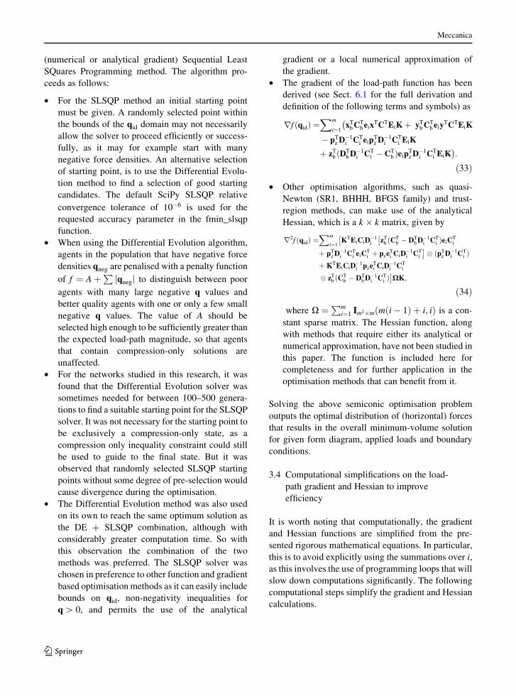
• The gradient of the load-path function has been

derived (see Sect. 6.1 for the full derivation and

definition of the following terms and symbols) as

rf ðqidÞ ¼Xm

i¼1xTbC

Tbeix

TCTEiKþ yTbCTbeiy

TCTEiK�

� pTzD�1i CT

i eipTzD

�1i CT

i EiK

þ zTb ðDTbD

�1i CT

i � CTb ÞeipTzD�1

i CTi EiK

�:

ð33Þ

• Other optimisation algorithms, such as quasi-

Newton (SR1, BHHH, BFGS family) and trust-

region methods, can make use of the analytical

Hessian, which is a k � k matrix, given by

r2f ðqidÞ ¼Xm

i¼1KTEiCiD

�1i zTb ðCT

b � DTbD

�1i CT

i ÞeiCTi

��

þ pTzD�1i CT

i eiCTi þ pze

Ti CiD

�1i CT

i

�� ðpTzD�1

i CTi Þ

þ KTEiCiD�1i pze

Ti CiD

�1i CT

i

� zTb ðCTb � DT

bD�1i CT

i Þ�XK;

ð34Þ

where X ¼Pm

i¼1 Im2�mðmði� 1Þ þ i; iÞ is a con-

stant sparse matrix. The Hessian function, along

with methods that require either its analytical or

numerical approximation, have not been studied in

this paper. The function is included here for

completeness and for further application in the

optimisation methods that can benefit from it.

Solving the above semiconic optimisation problem

outputs the optimal distribution of (horizontal) forces

that results in the overall minimum-volume solution

for given form diagram, applied loads and boundary

conditions.

3.4 Computational simplifications on the load-

path gradient and Hessian to improve

efficiency

It is worth noting that computationally, the gradient

and Hessian functions are simplified from the pre-

sented rigorous mathematical equations. In particular,

this is to avoid explicitly using the summations over i,

as this involves the use of programming loops that will

slow down computations significantly. The following

computational steps simplify the gradient and Hessian

calculations.

Meccanica

123

• If the summations are utilised and are programmed

as loop statements, it is recommended to use sparse

two-dimensional arrays where possible for the

sparsely populated matrices. This is especially true

for terms involving the multiplication of multiple

sparse matrices such as Db ¼ CTi QCb. For net-

works with higher numbers of elements, loop

statements may be time consuming to evaluate.

• Summation loops may be avoided by vectorising

the calculations. This may be performed by

recognising that the matrices used in the calcula-

tions are 2D of general size (a� b), and can be

stacked/tiled as slices into 3D arrays of size

(a� b� m) where m is the number of edges. For

the ei (m� 1) and Ei (m� m) arrays described

later in Sect. 6.1, these will be converted into

(m� 1� m) and (m� m� m) sized arrays,

respectively. The matrix calculations can then

proceed as normal with appropriate functions

supporting vectored input, with the summation

finally applied in a vectored manner to the final

arrays along the stacked dimension (third dimen-

sion in this case). Speed gains can be found with

larger arrays sizes with this vectorisation, but at the

cost of using arrays that consume more memory.

The X matrix for the Hessian can be pre-con-

structed and used in a similar manner.

• All of the terms that are independent of q, and so

do not vary with changes in qid, may be calculated

before the start of the optimisation process to avoid

spending time on recalculating arrays. This

includes individual vectors and matrices such as

x, C and pz, but also more complicated terms like

xTbCTbeix

TCTEiK.

4 Results

4.1 Grid comparisons

An orthogonal grid measuring ten by ten units and

with ten bays in each direction was studied. Unit point

loads were applied upwards at each vertex, with the

perimeter vertices fixed from translating in all direc-

tions and so forming the boundary vertices. There are

18 degrees-of-freedom in this network, one along each

row and column line of continuous edges. The

independent force densities were bounded in the range

(0, 10]. The calculated optimum solution with a load-

path of 449.4 is plotted in Fig. 4 and formed the base

solution for which to compare other solutions to. For

each of the example solutions presented in this section,

the number of function and gradient iterations for the

SLSQP solver is given in each figure caption, which

was used after 500 iterations of the differential

evolution solver to find a starting point.

The thrust network for the result in Fig. 4 is plotted

in Fig. 5, alongside the globally scaled (rmin) constant

force density solution. For the globally scaled uniform

force density case, the maximum rise of the thrust

network is 5.32, compared to 4.15 for the optimised

case. The comparison shows that the load-path, and

hence volume of the structure, was improved by 10%

Fig. 4 Form and force

diagrams for the resulting

optimised compression-only

force distribution for the

10 � 10 orthogonal grid,

with free vertices (white)

and boundary vertices

(blue). The thickness of the

red lines represents the area,

or magnitude of the internal

forces for given stress.

(Function evaluations: 1076,

Gradient evaluations: 52).

(Color figure online)

Meccanica

123

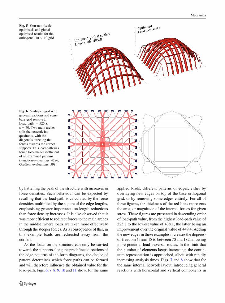
by flattening the peak of the structure with increases in

force densities. Such behaviour can be expected by

recalling that the load-path is calculated by the force

densities multiplied by the square of the edge lengths,

emphasising greater importance on length reductions

than force density increases. It is also observed that it

was more efficient to redirect forces to the main arches

in the middle, where loads are taken more effectively

through the steeper forces. As a consequence of this, in

this example loads are redirected away from the

corners.

As the loads on the structure can only be carried

towards the supports along the predefined directions of

the edge patterns of the form diagrams, the choice of

pattern determines which force paths can be formed

and will therefore influence the obtained value for the

load-path. Figs. 6, 7, 8, 9, 10 and 11 show, for the same

applied loads, different patterns of edges, either by

overlaying new edges on top of the base orthogonal

grid, or by removing some edges entirely. For all of

these figures, the thickness of the red lines represents

the area, or magnitude of the internal forces for given

stress. These figures are presented in descending order

of load-path value, from the highest load-path value of

525.8 to the lowest value of 438.1, the latter being an

improvement over the original value of 449.4. Adding

the new edges in these examples increases the degrees-

of-freedom k from 18 to between 70 and 182, allowing

more potential load traversal routes. In the limit that

the number of elements keeps increasing, the contin-

uum representation is approached, albeit with rapidly

increasing analysis times. Figs. 7 and 8 show that for

the same internal network layout, introducing general

reactions with horizontal and vertical components in

Fig. 5 Constant (scale

optimised) and global

optimised results for the

orthogonal 10 � 10 grid

Fig. 6 V-shaped grid with

general reactions and some

base grid removed:

Load-path ¼ 525:8,k ¼ 70. Two main arches

split the network into

quadrants, with the

diagonals directing the

forces towards the corner

supports. This load-path was

found to be the least efficient

of all examined patterns.

(Function evaluations: 4286,

Gradient evaluations: 59)

Meccanica

123

plan rather than just orthogonal reactions, can subtly

change the form and force diagrams for an improved

load-path.

4.2 General non-orthogonal network

The network in Fig. 12 possesses a general, non-

orthogonal form diagram and is relatively dense

with k ¼ 217. It consists of a triangulated network

supported along three boundary edges, and with

concentrated loading applied at the vertices based on

scaled area-weighted loads. The topology for this non-

orthogonal network was generated with a Delaunay

triangulation of a distribution of vertices along the

boundary and interior of the network. For analysis, a

combination of the Differential Evolution algorithm to

find a starting point was then followed by the function

and gradient SLSQP method. The allowable

force density range for the qid input was (0, 5], where

at the end of the analysis, the optimum load-path was

found to be 249.8 with a maximum independent

force density of 3.61. The main arching edge loops

can be seen spanning between the support lines, as

well as secondary main thrust lines forming within the

interior of the network. The associated thrust

network is plotted in Fig. 13, which took 13540

function evaluations and 215 gradient evaluations to

analyse.

Fig. 7 V-shaped grid with

orthogonal reactions:

Load-path ¼ 446:0,k ¼ 82. Diagonal edges

were overlaid onto the

orthogonal grid without any

edges removed, and showed

that an improvement in the

load-path could be found by

shedding some of the load

into a cross pattern at the

centre of the network.

(Function evaluations: 7020,

Gradient evaluations: 83)

Fig. 8 V-shaped grid with general reactions:

Load-path ¼ 445:4, k ¼ 118. By changing the supports in

Fig. 7 from taking only orthogonal reactions to general reactions

with components in both planar directions, a very slight

improvement was found. This can be attributed to allowing

thrusts coming at angles to the supports to be taken by the fixed

nodes and not from the orthogonal set of edges. (Function

evaluations: 7713, Gradient evaluations: 64)

Meccanica

123

5 Conclusions

This paper presented the derivation and implementa-

tion of a load-path optimisation method for discrete

thrust networks based on Thrust Network Analysis.

The internal and external load-path functions, which

are related to the volume and hence mass of the thrust

network elements, were derived for compression-only

structures. The geometry of these compression-only

thrust networks can be manipulated by assigning force

densities to the independent edges for a given set of

point loads and fixed boundary points on a common

plane.

The load-path concept was illustrated first with a

continuous and discrete parabolic arch example,

whereby the optimal height of the compression arch

was found by discrete scale optimisation. This method

determined the value of the scale factor of the form

and force diagrams that gave the minimum volume

solution for the discrete parabolic arch, mirroring the

analytical solution of the continuous case.

The external load-path function was laid out, along

with the associated gradient and Hessian functions for

use in optimisation solvers. A numerical implemen-

tation featuring the use of function and both function

and gradient-based solvers was used to determine the

general optimum load-path, so that spatial discretised

thrust networks could be tackled. A combination of

SLSQP and Differential Evolution solvers was used to

find the set of independent edge force densities that

Fig. 9 Diamond grid with general reactions:

Load-path ¼ 441:0, k ¼ 118. By changing the diagonal biased

networks of Figs. 7 and 8 into a diamond shaped network with

diagonals in both directions, a completely different pattern of

internal forces developed. Forces were found to move away

from the supports and form a larger diagonal shaped region in

the centre of the network. (Function evaluations: 9256, Gradient

evaluations: 75)

Fig. 10 Shifted diamond

grid with general reactions:

Load-path ¼ 440:5,k ¼ 118. By simply

translating the diamond

pattern of Fig. 9, a new force

distribution was found. This

can be seen as similar to the

pattern of Fig. 8, but with

additional diagonal

elements in the other

direction. (Function

evaluations: 9021, Gradient

evaluations: 74)

Meccanica

123

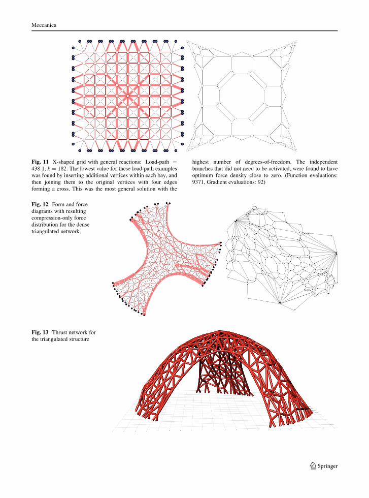
Fig. 11 X-shaped grid with general reactions: Load-path ¼438:1, k ¼ 182. The lowest value for these load-path examples

was found by inserting additional vertices within each bay, and

then joining them to the original vertices with four edges

forming a cross. This was the most general solution with the

highest number of degrees-of-freedom. The independent

branches that did not need to be activated, were found to have

optimum force density close to zero. (Function evaluations:

9371, Gradient evaluations: 92)

Fig. 12 Form and force

diagrams with resulting

compression-only force

distribution for the dense

triangulated network

Fig. 13 Thrust network for

the triangulated structure

Meccanica

123

minimised the load-path function subject to compres-

sion-only constraints.

A set of load-path optimised thrust networks were

compared that used the same loading state, with

differences in the pattern of additional overlaid edges

and whether the fixed vertex supports were orthogonal

or general. The comparisons showed that different

network topologies lead to different values of opti-

mised load-path function, with the efficiency depen-

dent on how well the network encourages the flow of

compression forces. The optimal solutions, when

compared with a discrete scaled uniform force density

solution, tended to have less overall rise and with

preference to shorter members rather than longer

members with higher force densities.

A further example demonstrating a general non-

orthogonal network showed that structures of high

network indeterminacy can be handled with the

current load-path implementation. The optimised

load-path method allows for the investigation of

efficient load carrying patterns for discrete networks,

so that they may be analysed for weight minimisation.

Acknowledgements The authors would like to acknowledge

William Baker for presenting the load-path concept to the

authors and for solving the optimal h / l ratio for the continuous

parabola.

Appendix

Gradient and Hessian derivation of the load-path

function

To calculate the gradient and Hessian of the external

load-path function in Eq. (31), the following common

matrix calculus properties are used, which follow [23]

Differential Calculus notation,

dAXB

dX¼BT � A ð35aÞ

dA�1

dA¼� ðA�T � A�1Þ; ð35bÞ

Note that this derivative is essentially a fourth-order

tensor, whose generic component represents the

derivative of the inverse of a matrix with respect to

its matrix. Let matrix functions f : Rn�k !Rm�pandg : Rn�k ! Rp�q then

df ðXÞ � gðXÞdX

¼ ðgðXÞT � ImÞf 0ðXÞ þ ðIq � f ðXÞÞg0ðXÞ;

ð35cÞ

where Im and Iq are the m� m; q� q identity matri-

ces, and� is the Kronecker matrix operator, defined as

the complete multiplication between two matrices i.e.

if A ðm� nÞ and B ðp� qÞ matrices, then A� B is an

ðmp� nqÞ matrix. Using the chain rule on the load-

path function, Equation (31) gives

df ðqidÞdqid

¼ df ðqidÞdQ

� dQdqid

ð36Þ

To find dQdqid

, notice that the diagonal matrix Q can

mathematically be written as a function of vector q

with

Q ¼Xm

i¼1

EiqeTi ; ð37Þ

where Ei is an m� m matrix with all its entries zero

except for identity in (i, i), and ei is an m� 1 vector

with identity on the ith element and zero everywhere

else. This derivative then becomes

dQ

dqid¼ d

Pmi¼1 Eiqe

Ti

dqid¼ d

Pmi¼1 EiKqide

Ti

dqid

¼Xm

1

ei � EiK

ð38Þ

¼Xm

1

Im2�mðmði� 1Þ þ i; iÞK ¼ XK; ð39Þ

where the matrix X is constructed by adding unity in

the aforementioned slots 8i, 1� i�m of the m2 � m

matrix I.

Now the derivativedf ðqidÞdQ of Eq. (36) is

df ðqidÞdQ

¼� ðpTz � pTz ÞðD�1i � D�1

i ÞðCTi � CT

i Þ

þ xTbCTb � xTCT þ yTbC

Tb � yTCT

� d pTzD�1i DbzbdQ

¼� pTzD�1i CT

i � pTzD�1i CT

i þ xTbCTb � xTCT

þ yTbCTb � yTCT � dpTzD

�1i DbzbdQ

ð40Þ

Meccanica

123

Note that the term D�1i Db is a function of qid if CiC

Ti

and is singular, i.e its spectral decomposition has a

diagonal matrix with at least one zero diagonal

element. The invariance of this term, in the case that

CiCTi is invertible, holds by

pTz ðCTi QCiÞ�1CT

i QCbzb

¼ pTz ðCTi QCiÞ�1CT

i QCiCTi ðCiC

Ti Þ

�1Cbzb

¼ pTzCTi ðCiC

Ti Þ

�1Cbzb:

ð41Þ

Assuming that CiCTi is not invertible, using Eq. (35c),

the derivative of pTzD�1i Dbzb is then

d½pTz ðCTi QCiÞ�1� � ðCT

i QCbzbÞdQ

¼ �ðzTbDTb � I1ÞðD�1

i CTi � pTzD

�1i CT

i Þþ ðI1 � pTzD

�1i ÞðzTbCT

b � CTi Þ

¼ �ðzTbDTbD

�1i CT

i Þ � ðpTzD�1i CT

i Þþ ðzTbCT

b Þ � ðpTzD�1i CT

i Þ¼ ½zTb ðCT

b � DTbD

�1i CT

i Þ� � ðpTzD�1i CT

i Þ:

ð42Þ

Thus,

df ðQÞdQ

¼� pTzD�1i CT

i � pTzD�1i CT

i þ xTbCTb � xTCT

þ yTbCTb � yTCT

� ½zTb ðCTb � DT

bD�1i CT

i Þ� � ðpTzD�1i CT

i Þ:ð43Þ

Inserting Eqs. (43) and (39) into (36) gives the 1� k

gradient of the load-path

rf ðqidÞ ¼df ðQÞdQ

� dQdqid

¼½�ðpTzD�1i CT

i � pTzD�1i CT

i Þ þ xTbCTb � xTCT

þ yTbCTb � yTCT

� ½zTb ðCTb � DT

bD�1i CT

i Þ� � ðpTzD�1i CT

i Þ� � XK¼Xm

i¼1xTbC

Tb eix

TCTEiKþ yTbCTb eiy

TCTEiK�

� pTzD�1i CT

i eipTzD

�1i CT

i EiK

þ zTb ðDTbD

�1i CT

i � CTb ÞeipTzD�1

i CTi EiK

�:

ð44Þ

In the same fashion, to determine the Hessian of the

function, the following chain rule is used

r2f ðqidÞ ¼drf

dQ� dQdqid

: ð45Þ

Note that one can temporarily ignore the sums of the

gradient, since dP

¼P

d, and consider them in the

final chain-rule calculation. The first two terms of

Equation (44) vanish in the Hessian, leaving only the

derivative

drf

dQ¼� d pTzD

�1i CT

i eipTzD

�1i CT

i EiK

dQ

þ d zTb ðDTbD

�1i CT

i � CTb ÞeipTzD�1

i CTi EiK

dQ:

ð46Þ

The first term of Eq. (46) by the multiplication rule is

equivalent to

dðpTzD�1i CT

i eiÞðpTzD�1i CT

i EiKÞdQ

ð47Þ

¼ �ðKTEiCiD�1i pz � I1Þ½eTi CiD

�1i CT

i � pTzD�1i CT

i �ð48Þ

� ðIk�k � pTzD�1i CT

i eiÞ½KTEiCiD�1i CT

i � pTzD�1i CT

i �ð49Þ

¼ � KTEiCiD�1i ðpzeTi CiD

�1i CT

i

�

þ pTzD�1i CT

i eiCTi Þ � pTzD

�1i CT

i

�:

ð50Þ

The second derivative of Eq. (46) is slightly more

complicated and is thus split in two parts

d zTbDTbD

�1i CT

i eipTzD

�1i CT

i EiK

dQð51Þ

d zTbCTbeip

TzD

�1i CT

i EiK

dQ: ð52Þ

Using Eqs. (35a) and (35b), the derivative (52)

becomes

�zTbCTbeiðKTEiCiD

�1i CT

i � pTzD�1i CT

i Þ: ð53Þ

Using the multiplication rule on Eq. (51) gives

dðzTbDTbD

�1i CT

i eiÞðpTzD�1i CT

i EiKÞdQ

ð54Þ

¼ ðKTEiCiD�1i pz � I1Þ½ðeTi CiD

�1i CT

i Þ� zTb ðCT

b � DTbD

�1i CT

i Þ�ð55Þ

Meccanica

123

� ðIk�k � zTbDTbD

�1i CT

i eiÞ½KTEiCiD�1i CT

i

� pTzD�1i CT

i � ð56Þ

¼ KTEiCiD�1i pze

Ti CiD

�1i CT

i � zTb ðCTb � DT

bD�1i CT

i Þð57Þ

� zTbDTbD

�1i CT

i eiðKTEiCiD�1i CT

i � pTzD�1i CT

i Þð58Þ

Putting (50), (58) and (53) together gives

drf

dQ¼Xm

i¼1KTEiCiD

�1i zTb ðCT

b � DTbD

�1i CT

i ÞeiCTi

��

þ pTzD�1i CT

i eiCTi þ pze

Ti CiD

�1i CT

i

�:

� ðpTzD�1i CT

i Þ þKTEiCiD�1i pze

Ti CiD

�1i CT

i

� zTb ðCTb � DT

bD�1i CT

i Þ�

ð59Þ

Finally, using Eq. (45) one gets the k � k Hessian

matrix of the load-path

r2f ðqidÞ ¼Xm

i¼1KTEiCiD

�1i zTb ðCT

b � DTbD

�1i CT

i ÞeiCTi

��

þ pTzD�1i CT

i eiCTi þ pze

Ti CiD

�1i CT

i �:� ðpTzD�1

i CTi Þ þKTEiCiD

�1i pze

Ti CiD

�1i CT

i

� zTb ðCTb � DT

bD�1i CT

i ��XK

¼Xm

j¼1

Xm

i¼1KTEiCiD

�1i zTb ðCT

b � DTbD

�1i CT

i ÞeiCTi

��

þ pTzD�1i CT

i eiCTi þ pze

Ti CiD

�1i CT

i

�ej:

�ðpTzD�1i CT

i EjKÞ þ ðKTEiCiD�1i pze

Ti CiD

�1i CT

i ejÞ� zTb ðCT

b � DTbD

�1i CT

i EiK�:

ð60Þ

All authors confirm/declare that they have no conflict

of interests with respect to the submitted research

project.

References

1. De Wilde WP (2006) Conceptual design of lightweight

structures: the role of morphological indicators and the

structural index. High Perform Struct Mater III WIT Trans

Built Environ 85:3–12

2. Vandenbergh T, De Wilde WP, Latteur P, Verbeeck B,

Ponsaert W, Van Steirteghem J (2006) Influence of stiffness

constraints on optimal design of trusses using morphologi-

cal indicators. High Performance Structures and Materials

III. WIT Trans Built Environ 85:31–40

3. Pyl L, Sitters CWM, De Wilde WP (2013) Design and

optimization of roof trusses using morphological indicators.

Adv Eng Softw 62–63:9–19

4. Mazurek A, Baker WF, Tort C (2011) Geometrical aspects

of optimum truss like structures. Struct Multidisciplinary

Optim 43(2):231–242

5. Baker WF, Beghini LL, Mazurek A, Carrion J, Beghini A

(2013) Maxwells reciprocal diagrams and discrete Michell

frames. Struct Multidisciplinary Optim 48(2):267–277

6. Beghini LL, Carrion J, Beghini A, Mazurek A, Baker WF

(2014) Structural optimization using graphic statics. Struct

Multidisciplinary Optim 49(3):351–366

7. Maxwell JC (1864) On reciprocal figures and diagrams of

forces. Philos Mag J Ser 4(27):250–261

8. Baker WF, Beghini A, Mazurek A (2012) Applications of

structural optimization in architectural design. In: 20th

analysis and computation speciality conference, pp 257–266

9. Block P, Ochsendorf J (2007) Thrust network analysis: a

new methodology for three-dimensional equilibrium. J Int

Assoc Shell Spat Struct 48(3):167–173

10. Block P (2009) Thrust network analysis: exploring three-

dimensional equilibrium. PhD dissertation, Massachusetts

Institute of Technology, Cambridge, USA

11. O’Dwyer DW (1999) Funicular analysis of masonry vaults.

Comput Struct 73:187–197

12. Fraternali F (2010) A thrust network approach to the equi-

librium problem of unreinforced masonry vaults via poly-

hedral stress functions. Mech Res Commun 37:198–204

13. Marmo F, Rosati L (2017) Reformulation and extension of

the thrust network analysis. Comput Struct 182:104–118

14. Linkwitz K, Schek HJ (1971) Einige Bemerkungen zur

Berechnung von vorgespannten Seilnetzkonstruktionen.

Ingenieur Archiv 40:145–158

15. Schek HJ (1974) The force density method for form finding

and computation of general networks. Comput Methods

Appl Mech Eng 3:115–134

16. Van Mele T, Rippmann M, Lachauer L, Block P (2012)

Geometry-based understanding of structures. J Int Assoc

Shell Spat Struct 53(2):285–295

17. Block P, Lachauer L (2014) Three-dimensional funicular

analysis of masonry vaults. Mech Res Commun 56:53–60

18. Van Mele T, Block P (2014) Algebraic graph statics.

Comput Aided Des 53:104–116

19. Van der Walt S, Colbert C, Varoquaux G (2011) The

NumPy array: a structure for efficient numerical computa-

tion. Comput Sci Eng 13:22–30

20. Jones E, Oliphant T, Peterson P, et al. (2001) SciPy: open

source scientific tools for Python, (Online; accessed

2017-02-13)

21. Python Software Foundation. Python Language Reference,

2016. Version 3.5

22. Storn R, Price K (1997) Differential evolution—a simple

and efficient heuristic for global optimization over contin-

uous spaces. J Glob Optim 11(4):341–359

23. Magnus JR, Neudecker H (1985) Matrix differential cal-

culus with applications to simple, hadamard, and kronecker

products. J Math Psychol 29(4):474–492

Meccanica

123