Linking Individual and Aggregate Price Changes*

Attila Rátfai†

Central European University

May 2003

Abstract

This paper develops an empirical model of price setting designed to capture the deviation

between the target and the actual price, and applies it to a unique panel data set of store level

retail prices. The aggregation of price deviations reveals that fluctuations in the shape of the

cross-sectional density of price deviations convey extra information on inflation dynamics.

Asymmetry in the density particularly matters. Idiosyncratic shocks alter the size but not the

direction of inflation fluctuations.

Key words: Inflation, (S,s) Pricing, Microeconomic Data, Simulated Maximum Likelihood

* For valuable discussions and suggestions at the early stage of this project I thank Matthew Shapiro. Robert Barsky, Susanto Basu, Ufuk Demiroglu, Gábor Körösi, Plutarchos Sakellaris, Todd Stinebrickner, and seminar participants at Bar-Ilan, Bocconi-IGIER, Ente Einaudi, Haifa, Hebrew U, Michigan, Southampton, Tel-Aviv, the 2002 Econometric Society European Meeting in Venice, the 2002 International Conference on Panel Data in Berlin, the 2002 ‘Summer at CEU’ Workshop in Budapest provided helpful insights to previous drafts. Ádám Reiff added excellent research assistance and useful comments. The usual caveat applies. † Department of Economics, Central European University, Nádor u. 9., Budapest 1051, Hungary, Email: ratfaia@ceu.hu

1

1 Introduction

Especially in countries having adopted inflation targeting as the focus of their monetary regime,

policymakers are seeking to possess advance knowledge of forthcoming price changes. Analysts

projecting the real returns on investment in financial assets are highly keen to learn about the

evolution of inflation rates. Despite its central importance for policy and business, however,

understanding the nature of short-term variation in inflation has been a daunting task for

economists for a long period of time.1

While a vast amount of research, mostly cast in univariate time-series models or Phillips

curve-type relationships has been amassed on the determinants of short-term inflation, recently

documented empirical regularities question the merit of existing approaches.2 First, for example,

in a review of standard macroeconomic indicators and forecasting techniques, Cecchetti (1995)

argues that forecasting relationships for aggregate inflation for the period 1982 to 1994 are

unstable and time varying. He concludes that the best, still highly imperfect predictor of inflation

appears to be its own past. Cecchetti and Groshen (2000) report on professional forecasters’

prediction of U.S. inflation rates: the standard deviation of the forecast error in one-year-ahead

forecast of inflation has been above 1 percent in the 1990s, while inflation averaged at about 3

percent. Atkison and Ohanian (2001) examine standard Phillips curve-based U.S. one-year ahead

inflation forecasts over the period of 1985 to 2000, and find that these models perform quite

poorly, even when compared to a simple random walk reference.

In principle, there are several ways to get around these disappointing developments. In

contrast to many related studies abstracting from microeconomic considerations and drawing on

aggregate (national or sector) level data, the present paper takes a step towards examining

inflation dynamics from a more structural, hitherto unexplored angle. In particular, it develops an

1 Short-term refers to horizons of one-month or one-quarter. 2 A detailed review of the traditional literature is beyond the scope of this study.

2

empirical model of pricing behavior that conforms to existing evidence on microeconomic

pricing patterns, and analyzes inflation through an explicit aggregation of store level price data.

By recognizing the importance of fixed price adjustment costs, the central object of the

analysis at the micro level is the price deviation, the postulated log difference between the actual

and the target price level.3,4 Potentially instrumental in related applications where lumpy and

heterogeneous microeconomic adjustment is relevant, the main insight of the paper in modeling

the price deviation is that a generalized two-sided (S,s) pricing policy naturally lends itself to a

trinomial latent variable interpretation of the microeconomic target price.5 Price deviations then

form price adjustment functions and cross-sectional price deviation densities, all of these objects

subsequently placed into an accounting framework to arrive at a measure of aggregate inflation.

Using the proposed machinery, three main issues of substance are investigated: the shape and the

intertemporal stability of adjustment functions and cross-sectional densities, the role of

fluctuations in price deviation densities in shaping inflation, and the importance of idiosyncratic

pricing shocks in inflation dynamics.

Besides the displeasing performance of existing methods, what motivates the specific

approach adopted in this study? First, direct store level evidence shows that nominal price

sequences exhibit relatively long periods of inaction followed by intermittent and discrete

adjustments. Lumpiness is coupled with a significant element of heterogeneity in the timing of

3 The target price is the optimal price when adjustment costs momentarily removed. Following the rest of the empirical (S,s) literature, the target is assumed to be proportional to the frictional price obtained as the solution to the optimal price setting problem with adjustment costs removed at all horizons. 4 What is dubbed price deviation here is often termed as relative or real price in related studies. The present terminology appears to better describe the behavioral concept at hand (cf. Caballero and Engel (1992)). 5 The non-smooth adjustment in nominal prices originates from fixed adjustment costs. See, for instance, Ball and Mankiw (1994) and (1995), Caballero and Engel (1992), Caplin and Leahy (1991), Dotsey et al (2000) and Tsiddon (1993).

3

price changes, especially across different stores.6 This description of the data in turn suggests

that two-sided (S,s) models are likely to serve as a particularly suitable framework for modeling

microeconomic pricing decisions.

Second, several recent studies have highlighted the importance of drawing on

microeconomic data in explaining the aggregate economy, when microeconomic behavior are

characterized by lumpiness and heterogeneity. For instance, Caballero, Engel and Haltiwanger

(1997) examine employment dynamics using a large microeconomic data set of firm-level data.

They find that changes in the cross-sectional density of the plant level deviation between actual

and target employment explains a sizeable portion of aggregate employment fluctuations in US

data. Drawing on the same data set, Caballero, Engel and Haltiwanger (1995) reach analogous

conclusions regarding capital demand and investment dynamics. Eberly (1994) shows that

simulated aggregate durable expenditures obtained from an explicit characterization of the cross-

section of heterogeneous and lumpy individual automobile purchase decisions are consistent

with the dynamics in aggregate durable expenditures in the United States in the early 1990s.

Overall, the upshot of this line of research is that it is vital to account for the degree of

coordination of lumpy and heterogeneous microeconomic actions in explaining the dynamics in

macroeconomic aggregates.

This paper is organized into five further sections. The retail price data set is introduced in

Section 2. The empirical model is developed in Section 3. The estimation procedure is outlined

in Section 4. Section 5 reports on the results and Section 6 concludes.

6 For a survey of the microeconomic evidence, see Wolman (2000). For more recent evidence, see Bils and Klenow (2002).

4

2 Data

Inferring the history of pricing shocks and their propagation through individual price sequences

to aggregate inflation requires a relatively long panel of microeconomic price data, ideally of

many homogenous products sold in several distinct stores. However, samples of prices that are

representative of finished goods markets at large or even of a specific sector of the economy are

rarely available in practice. Indeed, the shortage of appropriate store level price data may partly

explain the paucity of related research. To sidestep the data availability issue, this paper provides

a case study of a novel store level panel of retail prices.

The sample is a balanced panel of transaction prices of fourteen processed meat products

sold in eight different, geographically dispersed stores in Budapest, Hungary.7 Out of the eight

stores, five are larger department stores and three are smaller grocery stores, called Közért. All

stores sell many other products besides the ones considered here. Whenever a particular store is

visited, all the fourteen product prices are recorded. Observations in the sample are at the

monthly frequency, starting in January 1993 and ending in December 1996. Due to a five-month

intermission in data collection from April 1995 through September 1995, the sample is split into

two sub-periods covering 27 and 16 months. Throughout the sample period, there was no

government control of the product prices at hand.8

While having clear limitations in terms of its size and scope, the sample serves as an

excellent laboratory for the purposes of this study. First, the items are simple, well-defined,

important, homogeneous food products with essentially no variation in non-price, physical

characteristics such as quality. Second, the goods exhibit low degrees of processing; producing

them requires a single basic input component, the underlying raw material. Third, the items are

routinely purchased products with little variation in demand. Fourth, inference about stores’

7 The products are boneless chop, center chop, leg, back ribs, thin flank, round, roast, brisket, hot dog, sausage for boiling, shoulder, spare ribs, smoked loin-ham, fat bacon. 8 Appendix A provides further details of the sample. See also Rátfai (2003).

5

pricing policy is unlikely to be contaminated by major differences across production

technologies. Finally, although it is more volatile, the sample price index tracks movements in

the overall CPI, especially its food component. The partial correlation coefficient between the

sample average price level and the food component of the CPI in Hungary is 0.94. The time

series properties of the sample price index also closely match the properties of a similar sector

level index of processed meat product prices compiled by the Central Statistical Office, Hungary.

2.1 Descriptive Evidence

Rátfai (2003) provides a detailed non-parametric descriptive analysis of the data. To motivate the

empirical model of price setting, it is instructive to briefly highlight some basic findings therein.

First, nominal prices remain constant in 58 percent of the cases and the average duration of price

quotations is about three months with the longest spell being 17 months. With the exception of

months in the third quarter when the relevant raw material prices happen to spike, spells of

adjustment are spaced irregularly across stores. The duration of price changes within stores is

fairly dispersed over time, while contemporaneously it tends to be more synchronized.

The size of price changes is relatively homogenous across stores and products. The

average size of non-zero price changes is about 9 percent in the whole sample, with the largest

size being about 63 percent. The average size of positive changes is 10.85 percent in period 1

and 11.73 percent in period 2. Average negative changes are smaller: -8.24 percent in period 1

and -7.32 percent in period 2. These findings also suggest that price fixity can be well captured at

the monthly frequency.

6

3 The Empirical Model

The semi-structural model designed to capture the role of lumpiness and heterogeneity in

microeconomic pricing in inflation dynamics is developed in two stages. First, the

microeconomic model for the target price and the price deviation is specified. Then, an

aggregation framework is developed to organize price deviations into an inflation index9.

3.1 The Price Deviation

There exist a number of potential approaches to model the deviation between actual and

frictionless behavior. Caballero, Engel and Haltiwanger (1995), for instance, derive mandated

investment, the log deviation between actual and target capital as a function of firm-specific

variables that are individually highly persistent. They argue that an (S,s)-type decision rule

makes mandated investment mean-reverting, which in turn allows them to estimate the

parameters of mandated investment in a cointegrating framework. Alternatively, Caballero,

Engel and Haltiwanger (1997) identify the deviation between actual and target employment

through fluctuations in hours per worker, that they assume to be temporary. Finally, studies

examining the hypothesized correlation between the dispersion of cross-sectional price deviation

in microeconomic price data and inflation tend to proxy the target price with the cross-store

average of actual prices or the change in them (see Lach and Tsiddon (1992)). Besides the

absence of adequate theoretical foundations, the main concern with this ad hoc practice of

measurement is that identifying the target price with the product level average price hides the

distinction between idiosyncratic and aggregate pricing shocks.

The closest relative to the current approach are the ones explored in Bertola et al (2002)

and Sheshinski et al (1981). The differences between the current work and these other studies are

9 Throughout the analysis, aggregate inflation means the aggregate of price changes in the sample at hand.

7

still manifold. In short, Bertola et al (2002) implement one-sided (S,s) policies in estimating

microeconomic decision rules, abstract from the potential persistence in unobserved

heterogeneity, focus on a Tobit specification of decision rules and are mainly concerned with

microeconomic implications.10

The empirical framework developed in this paper markedly differs from previous

attempts to measure the deviation. It is based on the idea that fixed costs of changing prices

create an imbalance between actual and target behavior and make pricing policies state-

dependent. When shocks to the target price are symmetric, fixed adjustment costs result in a two-

sided (S,s) pricing rule with the price deviation, the log difference between the actual and the

target price typically differing from zero. Stores alter their nominal price and pay the fixed cost

only when the state variable, the price deviation is sufficiently large to exceed one of the

optimally determined threshold values. When shocks are unable to push the price deviation

outside the (S,s) band, the current nominal price coincides with the preceding one and no actual

pricing action takes place. That is, more formally, stores leave their nominal prices unaltered

until the price deviation in store i of product j at time t, zijt ≡ pij,t-1 - pijt*, passes one of the two

adjustment boundaries, S or s. If pricing shocks push zijt outside the band, stores will pay the

adjustment cost and alter their nominal price either upwards when zijt ≤ s or downwards when zijt

≥ S. The implied observation rule for the log nominal price level is then summarized as

*

, 1 , 1*

, 1 , 1*

, 1 , 1

ijt

p if p p Sij t ij t ijt

p p if s p p Sij t ij t ijt

p if p p sij t ij t ijt

< − > − − = < − < − − > − < − −

.

10 Sheshinski et al (1981) pursue a related latent variable approach in the pricing context.

8

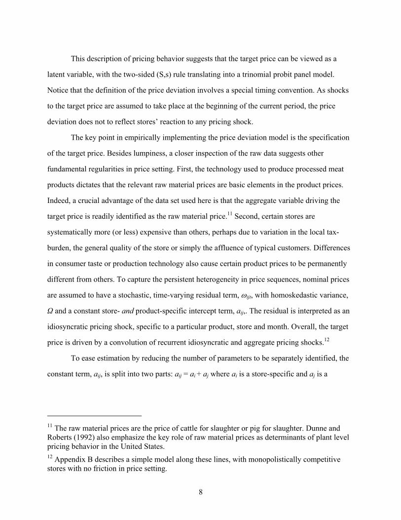
This description of pricing behavior suggests that the target price can be viewed as a

latent variable, with the two-sided (S,s) rule translating into a trinomial probit panel model.

Notice that the definition of the price deviation involves a special timing convention. As shocks

to the target price are assumed to take place at the beginning of the current period, the price

deviation does not to reflect stores’ reaction to any pricing shock.

The key point in empirically implementing the price deviation model is the specification

of the target price. Besides lumpiness, a closer inspection of the raw data suggests other

fundamental regularities in price setting. First, the technology used to produce processed meat

products dictates that the relevant raw material prices are basic elements in the product prices.

Indeed, a crucial advantage of the data set used here is that the aggregate variable driving the

target price is readily identified as the raw material price.11 Second, certain stores are

systematically more (or less) expensive than others, perhaps due to variation in the local tax-

burden, the general quality of the store or simply the affluence of typical customers. Differences

in consumer taste or production technology also cause certain product prices to be permanently

different from others. To capture the persistent heterogeneity in price sequences, nominal prices

are assumed to have a stochastic, time-varying residual term, ωijt, with homoskedastic variance,

Ω and a constant store- and product-specific intercept term, aij,. The residual is interpreted as an

idiosyncratic pricing shock, specific to a particular product, store and month. Overall, the target

price is driven by a convolution of recurrent idiosyncratic and aggregate pricing shocks.12

To ease estimation by reducing the number of parameters to be separately identified, the

constant term, aij, is split into two parts: aij = ai + aj where ai is a store-specific and aj is a

11 The raw material prices are the price of cattle for slaughter or pig for slaughter. Dunne and Roberts (1992) also emphasize the key role of raw material prices as determinants of plant level pricing behavior in the United States. 12 Appendix B describes a simple model along these lines, with monopolistically competitive stores with no friction in price setting.

9

product-specific component. Taken together, these considerations yield the following fixed effect

panel model for the log target price:

*ijt ij jt ijt i j jt ijtp a bm a a bmω ω= + + = + + + ,

where mjt denotes the log raw material price. Conforming to a model of optimal pricing decisions

in a monopolistically competitive market with no frictions, entry or exit, the economic

interpretation attached to this specification is one of markup over cost pricing. Overall, the

fundamental elements of the specification are flexible enough to encompass a large class of two-

sided (S,s) models.

3.2 State Dependence

The discrete choice decision rule associated with the latent variable framework exhibits both

what Heckman (1981a) calls true and spurious state-dependence. As the current realization of the

state variable is directly related to past actions, (S,s) type decision rules naturally give rise to true

state-dependence by the lagged control variable entering the decision rule via the censoring

thresholds. Spurious state dependence in general stems from the possibility that past realizations

of heterogeneous unobservables impact on current decision variables. This type of intertemporal

linkage appears here through serially correlated residuals, originating from persistent technology

or demand driven disturbances. To comply with this characterization of unobservables, the

residual term in the regression model is assumed to follow an AR(1) process, with a constant

auto-regressive parameter

ijttijijt ερωω += −1, ,

10

where εijt is N(0, σε2) i.i.d.. Overall, the resulting empirical model of the price deviation to be

estimated is a multi-period, trinomial, fixed effect panel Probit with serial correlation in the

residual.13

3.3 Aggregation

At the microeconomic level, aggregate and idiosyncratic pricing shocks are filtered through the

price deviation in a highly non-linear way. To capture the mechanism propagating

microeconomic pricing shocks to the aggregate level, an accounting framework defining a

measure of inflation as a weighted-average of the individual mean price changes with weights

given by the cross-sectional density of price deviations is introduced. Analogously to Caballero,

Engel and Haltiwanger (1995), (1997), omitting store- and product specific indices momentarily,

aggregate inflation is defined as

∫=Π tttttt dztzfzAz ),()( . (1)

The aggregation formula features two fundamental building blocks: the cross-sectional density of

price deviations, f(zt,t), and the price adjustment function, At(zt). The price adjustment function is

defined as the mean actual price change measured at particular realizations of price deviations

normalized by the corresponding price deviation. The main advantage of this particular

13 In general, the main advantage of a fixed over a random effect specification is that the former approach does not require the independence of latent heterogeneity and observed characteristics for consistent estimation. The main potential drawback of fixed effect specifications in many non-linear models is the incidental parameter problem: estimates of the individual effects are inconsistent for fixed T and this inconsistency is transmitted to other parameter estimates. Monte Carlo simulation results of a panel probit model in Heckman (1981b) indicate however that the bias is negligible in practice for N = 100 and T = 8; implying that inconsistency is unlikely to be a serious concern in the present application with N = 112, T = 27 or T = 16.

11

aggregation approach is that it allows for evaluating the role of fluctuations in price deviation

densities and adjustment functions in inflation dynamics. Potentially, it also permits to account

for the separate importance of idiosyncratic versus aggregate pricing shocks in inflation.14

4 Estimation

To motivate the estimation strategy, consider first the situation in which the residual in the model

for the price deviation developed above is identically and independently distributed. In the

absence of temporal dependence in the residual, the log-likelihood function can be simply

written as the product of the appropriate marginal probabilities

*

* *1

1,...,8 1,...,8 ( )1,..,14 1,...,14

ln ( ,..., ) ln ( )ijt ijt

ij ijT ijt i j jt ijti i p pj j

L prob p p f p a a bm dpτ= = =

= =

≡ = − − − =

∑ ∑ ∫

, 1 , 1

, 1

, 1 , 1

*

1,...,8 , 1 , 11,...,14

(1 ( )) ( )

ln( ( ) ( ( ))

ijt ij t ijt ij t

ijt ij t

ij t i j jt ij t i j jtp p p p

ijti ij t i j jt ij t i j jtj p p

F p s a a bm F p S a a bm

dpF p s a a bm F p S a a bm

− −

−

− −∞> <

= −∞ − −= =

− − − − − × − − − − ×

− − − − − − − − −

∏ ∏∑ ∫ ∏

where F(.) denotes the normal cumulative density function. Here standard quadrature based

Maximum Likelihood procedures serve as a straightforward solution method. Even if temporal

dependence in the error term is neglected when it is actually present, parameter estimates are

consistent.15

However, if the correlation structure is erroneously specified as i.i.d., and lagged

dependent variables enter the model as they do here via the censoring thresholds, the standard

14 The resulting weighted measure of inflation is plotted in Figure 1b. It is virtually identical to the unweighted index of aggregate price changes as shown in Figure 1a. The correlation coefficient is 0.998. 15 Nonetheless, parameter estimates and the estimated standard errors are biased.

12

ML estimation of the probit panel model leads to inconsistent parameter estimates (see Keane

(1993)). This concern is especially troubling in the present application as the estimated

parameters are used to form the cross-sectional density of price deviations and then aggregate

inflation. These considerations call for a more careful treatment of the serial correlation in the

residual. Once this is done, however, the log-likelihood function cannot be factored out in the

usual fashion as evaluating the joint likelihood of consecutive price observations requires the

computation of T (the number of time periods) dimensional integrals. Without imposing further

simplifying restrictions on the covariance structure of residuals, the computation of these high

dimensional integrals is numerically infeasible by standard procedures. Fortunately, simulation

estimation techniques offer a suitable remedy.

A simple approach to consistently estimate model parameters is the direct simulation of

choice sequence probabilities by the observed frequencies (Lerman and Manski (1981)). The

problem with the direct simulation approach is that obtaining reasonably precise estimates of the

possibly quite small probabilities entails a burdensome number of draws and thus excessive

computational efforts. In the absence of a large number of draws, the frequency simulator of the

joint choice probabilities is discontinuous in the estimated parameters.16

The Simulated Maximum Likelihood (SML) estimator drawing on the Geweke-

Hajivassiliou-Keane (GHK) simulator of importance sampling of univariate truncated normal

variates offers a viable alternative. A brief outline of the GHK procedure tailored to the present

context is as follows. The log-likelihood function to be maximized is

*

* *1

1,...,8 1,...,8 ( )1,..,14 1,...,14

ln ( ,..., ) ln ( )ijt ijt

ij ijT ijt i j jt ijti i p pj j

L prob p p f p a a bm dpτ= = =

= =

≡ = − − −

∑ ∑ ∫ .

16 Indeed, besides computational feasibility, smoothness (differentiability and continuousness) is a fundamental requirement to simulation estimators as it allows for applying standard hill-climbing or gradient methods in maximizing the log-likelihood function.

13

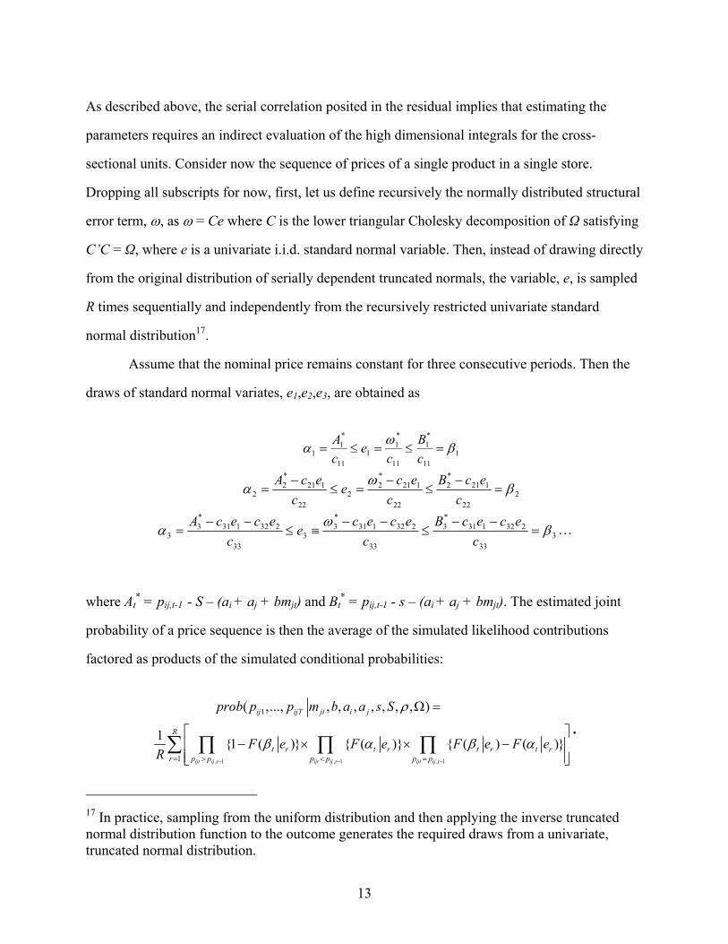
As described above, the serial correlation posited in the residual implies that estimating the

parameters requires an indirect evaluation of the high dimensional integrals for the cross-

sectional units. Consider now the sequence of prices of a single product in a single store.

Dropping all subscripts for now, first, let us define recursively the normally distributed structural

error term, ω, as ω = Ce where C is the lower triangular Cholesky decomposition of Ω satisfying

C’C = Ω, where e is a univariate i.i.d. standard normal variable. Then, instead of drawing directly

from the original distribution of serially dependent truncated normals, the variable, e, is sampled

R times sequentially and independently from the recursively restricted univariate standard

normal distribution17.

Assume that the nominal price remains constant for three consecutive periods. Then the

draws of standard normal variates, e1,e2,e3, are obtained as

111

*1

11

*1

111

*1

1 βωα =≤=≤=cB

ce

cA

222

121*2

22

121*2

222

121*2

2 βω

α =−

≤−

=≤−

=c

ecBc

ecec

ecA

333

232131*3

33

232131*3

333

232131*3

3 βω

α =−−

≤−−

≡≤−−

=c

ececBc

ececec

ececA …

where At* = pij,t-1 - S – (ai + aj + bmjt) and Bt

* = pij,t-1 - s – (ai + aj + bmjt). The estimated joint

probability of a price sequence is then the average of the simulated likelihood contributions

factored as products of the simulated conditional probabilities:

, 1 , 1 , 1

1

1

( ,..., , , , , , , , )

1 1 ( ) ( ) ( ) ( )ijt ij t ijt ij t ijt ij t

ij ijT jt i j

R

t r t r t r t rr p p p p p p

prob p p m b a a s S

F e F e F e F eR

ρ

β α β α− − −= > < =

Ω =

− × × −

∑ ∏ ∏ ∏

.

17 In practice, sampling from the uniform distribution and then applying the inverse truncated normal distribution function to the outcome generates the required draws from a univariate, truncated normal distribution.

14

The computationally burdensome stage of the estimation is the large number of simulations to

estimate the joint occurrence of a sequence of price realizations. Börsch-Supan and Hajivassiliou

(1993) report that relatively accurate likelihood estimates are obtained by employing a relatively

small number of repetitive draws; 20 or 30 draws are often sufficient with three to seven

alternative choices. In the current application, to use err at the conservative end, 50 sampling

draws are employed. Although estimates of the implied truncated residuals are in general biased,

the likelihood contribution is correctly simulated. Most importantly, the simulated log-likelihood

is an unbiased and smooth estimate of the true log-likelihood function.18

Identification of the intercept effects requires fixing at least one of the adjustment

boundary parameters. While its exact position being constrained, the size of the band is still

determined independently of this restriction. The initial values used in the simulation estimation

are obtained from estimating the model with no serial correlation in the residual.

Experimentation with alternative initial values confirms that the estimation results are robust to

reasonable departures from these particular values.

Separately for the two periods, the estimated parameters of interest are reported in Table

1.19 There are some notable points to highlight. First, the standard errors indicate that the

parameters are fairly tightly estimated. Second, the autocorrelation parameters are sizeable and

significantly different from zero, justifying the explicit account for the temporal dependence in

18 Extensive comparisons by Börsch-Supan and Hajivassiliou (1993) of the accuracy and bias in the various possible simulation estimators of multivariate truncated normal probabilities show that the GHK approach performs best among similar estimators. Besides accommodating various correlation structures, the SML estimator is continuous in the parameters, relatively quick in reaching convergence, and provides consistent and efficient estimates even in the presence of lagged endogenous variables. 19 The estimations are performed in Gauss. The routine draws on a code simulating multivariate normal probabilities in a multinomial probit model supplied by Vassilis Hajivassiliou via his anonymous ftp-site. The parameter for the upper boundary is set to S = 0.13 in both periods. The results are robust to including monthly dummies in the baseline specification.

15

the unobserved residual. Third, the slope estimates are somewhat larger than one indicating some

increasing returns at the micro level. Fourth, the implied total size of the band is about 35% and

26% in the two periods. Finally, with the exception of the band parameters, the important point

estimates in the two periods are about the same.

5 Results

5.1.1 The Cross-Sectional Density of Price Deviations

One of the fundamental implications of state dependent pricing models is that the impact of

pricing shocks on aggregate price changes depends on the cross-sectional distribution of price

deviations. In aggregating (S,s) pricing policies, Caplin and Spulber (1986) assume a uniform

time-invariant distribution of price deviations and conclude that expected monetary policy may

have no impact on aggregate output even when prices are sticky. Tsiddon (1993) demonstrates in

a two-sided (S,s) pricing model that a positive trend in the target price forces price deviations to

spend disproportionately more time closer to the lower adjustment band than to the upper one.

The pressure exerted by the positive trend thus implies that the stationary distribution of price

deviations has an asymmetric, in Tsiddon (1993) piece-wise exponential shape.

The sample of product prices used in this study appears to be ideal to learn more about

the shape of price deviation densities observed in the data. To generate the empirical densities,

one first needs to obtain an estimate of idiosyncratic shocks. While the exact realization of

idiosyncratic shocks is directly unobserved by construction, their density is readily available. To

obtain the probabilities defining the truncated densities, first, a discretized state space is defined

with a bin width of one percent for price deviations between –70 and 60 percents. The

conditional probabilities generating the truncated densities are evaluated at the middle-point of

the bin intervals. Given the truncation points of Aijt* = pij,t-1 - S – (ai + aj + bmjt) and Bijt

* = pij,t-1 -

16

s – (ai + aj + bmjt), the probabilities defining the truncated normal densities are then obtained as

the ratios of the probability of being in a particular bin interval and the probability of

experiencing a particular pricing action. Averaging then the resulting truncated densities in the

cross-section results in an empirical distribution of price deviations in each month.

Microeconomic price deviations are constructed by imposing a microeconomic decision

rule of the (S,s) type on the data. Is the shape of the resulting empirical densities consistent with

any of the possible approaches to aggregating microeconomic (S,s) pricing rules? First, summary

statistics show that the average standard deviation of price deviations in the sample is 15.23

percent, reflecting the fact that there is considerable cross-sectional heterogeneity in pricing both

across stores and products. The two panels in Figure 2 show the histogram of price deviations in

the two periods, pooled over time, stores and products20. The density appears to be highly non-

uniform and asymmetric, consistently with the presumption made in aggregating two-sided (S,s)

policies.

How does the shape of the empirical densities of price deviations evolve over time? To

ease visual interpretation, first, the quarterly frequency densities are displayed in Figure 3.

Simple eyeballing of the graphs indicates that the densities tend to have non-uniform, often

asymmetric shape. Histograms in the third quarter tend to feature leftward warped distributions

with many price deviations bunching towards the lower end of the density. This shape of the

distribution is consistent with the presence of strong inflationary pressures. Conversely, the

rightward bent second quarter histograms typically reflect the pressure on nominal price cuts.

Changes in the shape of the histograms are suggestive of the evolution of aggregate

inflation. A few interesting episodes indeed stand out. By many price deviations bunching in the

neighborhood of the lower adjustment boundary, the histograms in Figure 3 pick up the story of

accelerating inflation in early 1994 eventually terminated by the middle of 1995. Also, the

relatively large number of price deviations bunching on the right end of the densities at the

20 To facilitate visual inspection, a third degree polynomial is fitted to all empirical densities.

17

beginning of 1993 and 1996 witness deflationary pressures on meat product prices. In contrast, in

the first part of 1994, the histograms rather signal pressure on subsequent price increases.

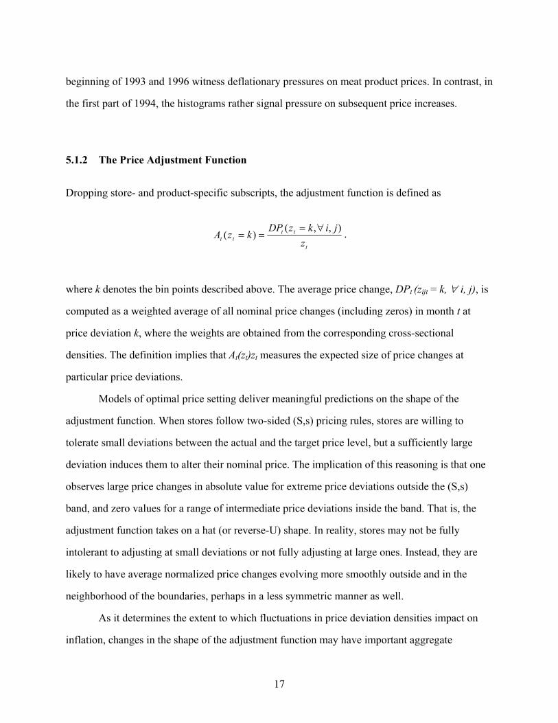
5.1.2 The Price Adjustment Function

Dropping store- and product-specific subscripts, the adjustment function is defined as

t

tttt z

jikzDPkzA

),,()(

∀=== .

where k denotes the bin points described above. The average price change, DPt (zijt = k, ∀ i, j), is

computed as a weighted average of all nominal price changes (including zeros) in month t at

price deviation k, where the weights are obtained from the corresponding cross-sectional

densities. The definition implies that At(zt)zt measures the expected size of price changes at

particular price deviations.

Models of optimal price setting deliver meaningful predictions on the shape of the

adjustment function. When stores follow two-sided (S,s) pricing rules, stores are willing to

tolerate small deviations between the actual and the target price level, but a sufficiently large

deviation induces them to alter their nominal price. The implication of this reasoning is that one

observes large price changes in absolute value for extreme price deviations outside the (S,s)

band, and zero values for a range of intermediate price deviations inside the band. That is, the

adjustment function takes on a hat (or reverse-U) shape. In reality, stores may not be fully

intolerant to adjusting at small deviations or not fully adjusting at large ones. Instead, they are

likely to have average normalized price changes evolving more smoothly outside and in the

neighborhood of the boundaries, perhaps in a less symmetric manner as well.

As it determines the extent to which fluctuations in price deviation densities impact on

inflation, changes in the shape of the adjustment function may have important aggregate

18

consequences. If the adjustment function is assumed to be an nth degree polynomial then

aggregate inflation depends on all the (n+1) moments of price deviations (see Caballero, Engel

and Haltiwanger (1995), (1997)). For instance, if adjustment costs were nonexistent or simply

convex, At(zt) would follow a smooth path and be virtually invariant to zt. Then higher moments

of the cross-sectional density of price deviations would be irrelevant to inflation.

Figure 4 portrays the total adjustment functions, separately for the two periods. The

functions are constructed by pooling all price deviations in the two parts of the sample. Visual

inspection of the graphs suggests that the shape of the adjustment functions is in general

consistent with the implication of two-sided (S,s) models, taking on a hat-shaped form and

reflecting the inaction region implied by the latent variable structure imposed on the data.21 It is

also apparent that the average adjustment functions are relatively stable across the quarters.

Figure 5 displays the same information separately for the fourteen quarters available.

Despite the noise in constructing the graphs, the pictures again indicate that adjustment functions

are remarkably stable over time and that they are broadly consistent with (S,s) theory motivating

their construction. The intertemporal stability of the adjustment function indicates that the

empirical specification imposed on the data captures well the underlying microeconomic

structure governing stores’ pricing behavior.

5.2 Aggregate Implications

With fixed price adjustment costs, histories of pricing shocks and the heterogeneous response of

stores to these shocks are summarized in the cross-sectional density of price deviations, implying

that the shape of these densities is likely to serve as an important determinant of aggregate price

dynamics. Drawing on sector level inflation data in the U.S., Ball and Mankiw (1995) indeed

21 The discontinuity is due to the assumption that the boundaries are fixed.

19

find that the higher moments of cross-sector relative inflation rate densities impact on inflation.

They conclude that inflation is primarily related to the asymmetry in the distribution.

The following analysis also asks how the shape of microeconomic price deviation

densities determines inflation dynamics. The main focus of analysis is on the dispersion and

asymmetry in the densities. Dispersion is captured by the standard deviation statistic. Measuring

asymmetry is less straightforward; it is not a priori obvious what statistic captures best the

fundamental concept of interest, the relative bunching of price deviations near to the adjustment

boundaries. In what follows two alternative measures of asymmetry are considered, the standard

skewness coefficient and the mean-median difference.

First, the three panels in Figure 6 show the time path of the dispersion and asymmetry

measures along with the corresponding aggregate inflation series. The graphs suggest that

inflation is positively correlated with all the three different measures of the shape of the density.

Table 2 displaying the unconditional correlation coefficient among the series confirms this

presumption. Moreover, the correlation is sizeable and significant for both asymmetry measures.

To assess the robustness of the simple correlation results, conforming to Ball and

Mankiw (1995), a set of horse-race regressions is run with aggregate inflation as the dependent

and the various measures of the shape of price deviation densities as independent variables.

While the specification is clearly simple, it highlights the role higher moments of price deviation

densities may play in inflation dynamics. The basic regression equation takes the form of

0 1 1 2 3( ) ( )t t t t tb b b StDev z b Asym z u−Π = + Π + + +

where StDev(z) denotes the standard deviation and Asym(z) denotes the asymmetry measure of

price deviation densities.

Six different specifications are considered. All of them include a constant, lagged

inflation and measures of the shape of price deviation densities as explanatory variables. The

findings are summarized in Table 3. Estimates from the benchmark AR(1) model reported in the

20

first column. The coefficient on the lagged inflation term points to the persistence in the inflation

process. The R2 statistic indicates a respectable fit. The second column shows results with a

model appended with the standard deviation in price deviations. Comparing the adjusted R2

statistics reported in the first two columns indicates that adding the standard deviation provides

no progress in goodness-of-fit and the standard deviation parameter is insignificant. The results

for the equation augmented solely by the skewness statistic are displayed in the third column.

This specification substantially improves goodness-of-fit when compared to the preceding ones.

In addition, the parameter estimates for skewness are statistically significant. The findings for the

model that includes both skewness and standard deviation as independent variables are in

column five. Having measures of both dispersion and skewness in the regression equation leaves

the standard deviation parameter insignificant and the fit of the model virtually unchanged. The

final two models use the alternative measure of asymmetry in the price deviation distribution, the

mean-median difference. The results show that the parameter estimates are of the expected sign,

the ones for the asymmetry measure are statistically significant. The models with or without the

standard deviation provide a better fit than either the AR(1) or the pure standard deviation model,

but a poorer fit then implied by the models with the skewness statistic.

It is instructive to examine how fluctuations in At(zt) and f(z,t) shape inflation dynamics

from yet another angle. The idea is to construct counterfactual aggregate inflation series by

replacing the actual monthly frequency cross-sectional distributions and adjustment functions

with their seasonal (i.e. quarterly) or overall average counterpart, and then compare the

proximity of these counterfactual series with the true one. For example, replacing the actual

adjustment function, At(zt) in the aggregating framework with the corresponding seasonal

average amounts to shutting down cyclical but retaining seasonal fluctuations in it. Following

Caballero, Engel and Haltiwanger (1997), the goodness-of-fit measure used to evaluate the

proximity of the resulting counterfactual and actual price dynamics is

21

)()(1(.) 2

2

t

tcftGΠ

Π−Π−=

σσ

where Πtcf (cf = s (seasonal), oa (overall average)) is the counterfactual, Πt is the actual aggregate

price change and σ2 denotes the time-series variance of the series. To the extent that it is not

constrained by zero from below, the statistic is different from the traditional goodness-of-fit

measure, R2.22

Table 4 displays the goodness-of-fit results. First, shutting down cyclical and keeping

only seasonal movements in f(z,t) distracts aggregate inflation from its true dynamics by a much

larger extent than playing down similar cyclical fluctuations in At(zt). In the former case,

reflecting again the intertemporal stability of the adjustment function, G(.) falls by 26 percent,

while in the latter case only by 10 percent. Entries in the top right and bottom left corner of the

table show the goodness-of-fit measures obtained by removing all (seasonal and non-seasonal)

fluctuations in the cross-sectional density or in the adjustment function, respectively. The results

indicate a dramatic deterioration in fit in the former case, G(.) falling to 0.37. In contrast, the

proximity of the two series is only moderately reduced with no time-series variation in the

adjustment function. The goodness-of-fit statistic is 0.79 here. Indeed, removing all fluctuations

in the adjustment function and keeping the original density results in a better fit than taking away

only cyclical and leaving seasonal fluctuations in the cross-sectional distributions.

The results overall indicate that swings in both the cross-sectional density and the

adjustment function are non-trivial ingredients of aggregate price dynamics. Seasonal and

cyclical fluctuations in the adjustment function contribute relatively little to aggregate price

dynamics, while fluctuations in the cross-sectional distribution are fundamental both at the

seasonal and the cyclical frequency.

22 The reason for this is that the residual part here is not necessarily uncorrelated with the predicted one.

22

5.3 Idiosyncratic Shocks

In a frictionless neoclassical economy the aggregate impact of idiosyncratic shocks cancels out

by relative price adjustment. Although they still average to zero by definition, the impact of

idiosyncratic shocks on pricing decisions is not neutral any more if there are fixed costs to price

adjustment. Many small idiosyncratic shocks in one direction may have no aggregate effect at

all, while only a few large ones in one direction actually does have.

How important idiosyncratic shocks are in shaping aggregate price dynamics? In

particular, what fraction of fluctuations in inflation can be attributed to idiosyncratic shocks,

after having them filtered through the cross-sectional density of price deviations?23 To address

this issue, first, idiosyncratic shocks are suppressed in computing the counterfactual price

deviation densities, f(y), under the maintained assumption that adjustment functions remain the

same as in the baseline case, A(a). Then the counterfactual inflation series are obtained as a

weighted average of price changes with weights provided by f(y).

Figure 7 displays the counterfactual series together with the actual one. A simple visual

inspection of the graph suggests that the series closely moves together. This impression is

confirmed by the partial correlation coefficient of 0.88. Figure 7 also suggests that idiosyncratic

shocks alter the size of inflation changes. Had idiosyncratic shocks not mitigated aggregate

surprises, for instance, inflation would have been higher by 3 to 9 percents between July and

October 1994. At the same time, during the first six months of 1993 idiosyncratic shocks seem to

have prevented an even more drastic deflation in processed meat product prices. The proximity

of the true and the counterfactual series is also assessed by the goodness-of-fit statistic

introduced earlier. The resulting figure of 0.62 indicates that eliminating all variation in

idiosyncratic disturbances fundamentally alters the size of inflation changes, though not their

23 Idiosyncratic shocks are identified with the residual obtained in the panel model. Eliminating idiosyncratic shocks means that the only source of heterogeneity in counterfactual price deviations stems from the time-invariant individual effects.

23

direction. Finally, Figure 8 displays the empirical density when price deviations are fully purged

from idiosyncratic shocks. The graph features a non-uniform distribution suggesting that it is not

the particular functional form imposed on the residual term that drives the basic shape of price

deviation densities.

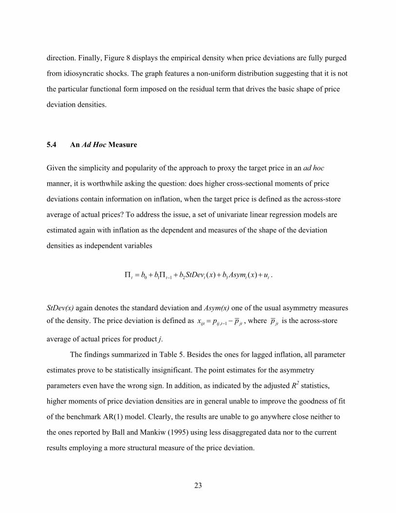
5.4 An Ad Hoc Measure

Given the simplicity and popularity of the approach to proxy the target price in an ad hoc

manner, it is worthwhile asking the question: does higher cross-sectional moments of price

deviations contain information on inflation, when the target price is defined as the across-store

average of actual prices? To address the issue, a set of univariate linear regression models are

estimated again with inflation as the dependent and measures of the shape of the deviation

densities as independent variables

0 1 1 2 3( ) ( )t t t t tb b b StDev x b Asym x u−Π = + Π + + + .

StDev(x) again denotes the standard deviation and Asym(x) one of the usual asymmetry measures of the density. The price deviation is defined as , 1ijt ij t jtx p p−= − , where jtp is the across-store

average of actual prices for product j.

The findings summarized in Table 5. Besides the ones for lagged inflation, all parameter

estimates prove to be statistically insignificant. The point estimates for the asymmetry

parameters even have the wrong sign. In addition, as indicated by the adjusted R2 statistics,

higher moments of price deviation densities are in general unable to improve the goodness of fit

of the benchmark AR(1) model. Clearly, the results are unable to go anywhere close neither to

the ones reported by Ball and Mankiw (1995) using less disaggregated data nor to the current

results employing a more structural measure of the price deviation.

24

6 Conclusions

Are (S,s) pricing models originally designed to provide behavioral foundations for business cycle

analysis able to carry implications for the understanding of inflation dynamics? By applying an

empirical technique rooted directly in (S,s) considerations to a unique, highly disaggregated

panel sample of consumer prices, the study gives an affirmative answer.

The empirical model is specifically aimed at recovering and quantifying information

potentially lost by merely taking averages of individual prices when modeling inflation

determination. What can one carry away from the analysis? The findings in general confirm the

argument that an explicit aggregation of intermittent and heterogeneous individual pricing

actions yields new insights for a more adequate understanding of aggregate price changes. More

in particular, first, the shape of the price adjustment function is relatively stable over time.

Second, fluctuations in the shape of the cross-sectional distribution of price deviations contribute

to aggregate inflation dynamics. Asymmetry in the cross-sectional density particularly matters.

Finally, though idiosyncratic shocks do not alter the direction of aggregate inflation dynamics,

they do determine the magnitude of fluctuations.

Provided that the appropriate microeconomic price data are available on a timely basis,

the analysis also has clear implications for monetary policy making. In formulating short-term

inflation forecasts, central banks currently rely on only histories of aggregate variables, often

mainly inflation itself. Prior evidence indicates however that the usual macroeconomic variables

are unable to reliably forecast short-term aggregate price changes. In contrast, the findings of this

study show that even when no particular pattern is observed in past average prices, the latent

pressure built up in directly unobservable price deviations can provide a useful signal for

forthcoming inflation. In practice, detecting the correct signal requires a careful specification of

25

the target price for the product prices at hand and a forecasting procedure that accounts for the

specific features of the timing of microeconomic data release.24

Finally, a clear limitation of the analysis is the specificity and the size of the sample.

Future research should also investigate a richer sample of prices with a broader set of product

categories and more stores involved.

24 Implications of the model for out-of-sample forecasting are the subject of ongoing research.

26

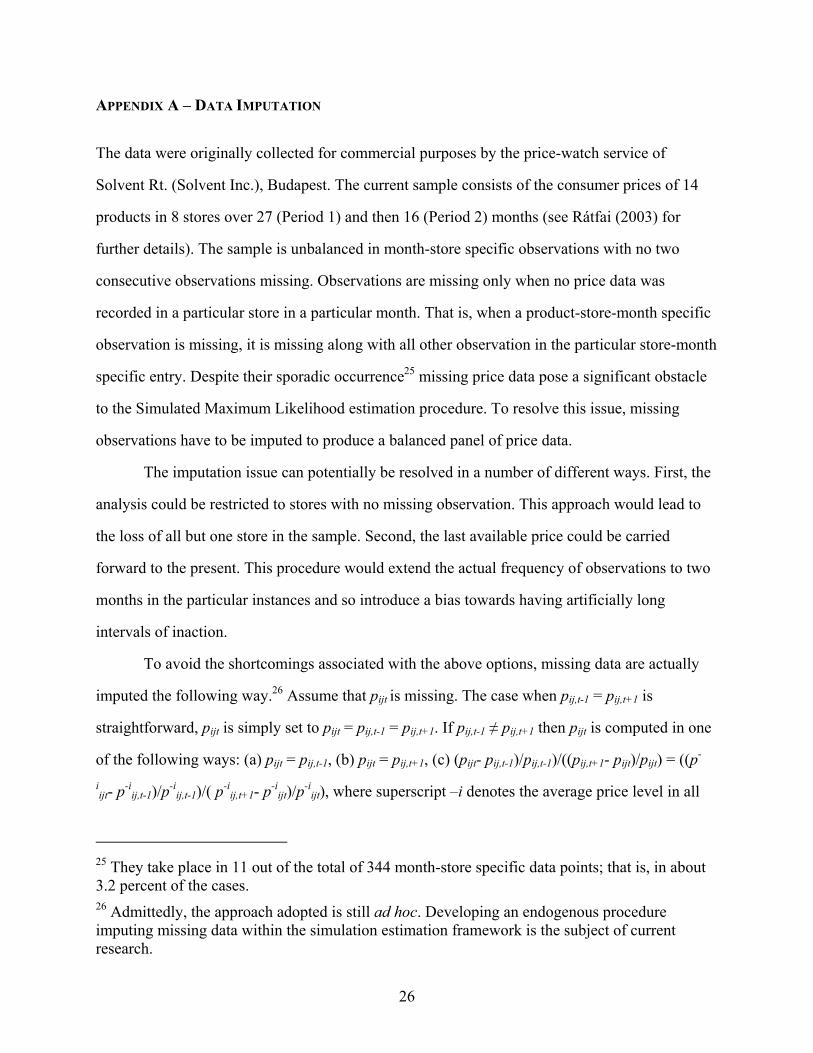
APPENDIX A – DATA IMPUTATION

The data were originally collected for commercial purposes by the price-watch service of

Solvent Rt. (Solvent Inc.), Budapest. The current sample consists of the consumer prices of 14

products in 8 stores over 27 (Period 1) and then 16 (Period 2) months (see Rátfai (2003) for

further details). The sample is unbalanced in month-store specific observations with no two

consecutive observations missing. Observations are missing only when no price data was

recorded in a particular store in a particular month. That is, when a product-store-month specific

observation is missing, it is missing along with all other observation in the particular store-month

specific entry. Despite their sporadic occurrence25 missing price data pose a significant obstacle

to the Simulated Maximum Likelihood estimation procedure. To resolve this issue, missing

observations have to be imputed to produce a balanced panel of price data.

The imputation issue can potentially be resolved in a number of different ways. First, the

analysis could be restricted to stores with no missing observation. This approach would lead to

the loss of all but one store in the sample. Second, the last available price could be carried

forward to the present. This procedure would extend the actual frequency of observations to two

months in the particular instances and so introduce a bias towards having artificially long

intervals of inaction.

To avoid the shortcomings associated with the above options, missing data are actually

imputed the following way.26 Assume that pijt is missing. The case when pij,t-1 = pij,t+1 is

straightforward, pijt is simply set to pijt = pij,t-1 = pij,t+1. If pij,t-1 ≠ pij,t+1 then pijt is computed in one

of the following ways: (a) pijt = pij,t-1, (b) pijt = pij,t+1, (c) (pijt- pij,t-1)/pij,t-1)/((pij,t+1- pijt)/pijt) = ((p-

iijt- p-i

ij,t-1)/p-iij,t-1)/( p-i

ij,t+1- p-iijt)/p-i

ijt), where superscript –i denotes the average price level in all

25 They take place in 11 out of the total of 344 month-store specific data points; that is, in about 3.2 percent of the cases. 26 Admittedly, the approach adopted is still ad hoc. Developing an endogenous procedure imputing missing data within the simulation estimation framework is the subject of current research.

27

the stores but store i. If the number of non-missing price changes between period t-1 and t and

between t and t+1 in all stores other than store i exceeds the number of unchanged prices in these

periods then option (c) is selected. This approach is based on the implicit assumption that the

ratio of the unobserved price changes between periods t-1 and t and periods t and t+1 in store i

corresponds to the similar ratio of the average of non-missing price changes.

If the number of non-missing price changes between period t-1 and t and between t and

t+1 does not exceed the number of unchanged prices then the choice is between the first options

(a) and (b). Option (a) is selected if the number of pairs of non-missing observations with price

fixity between month t-1 and t outnumbers the number of similar cases between month t and t+1.

Otherwise, option (b) is selected.

28

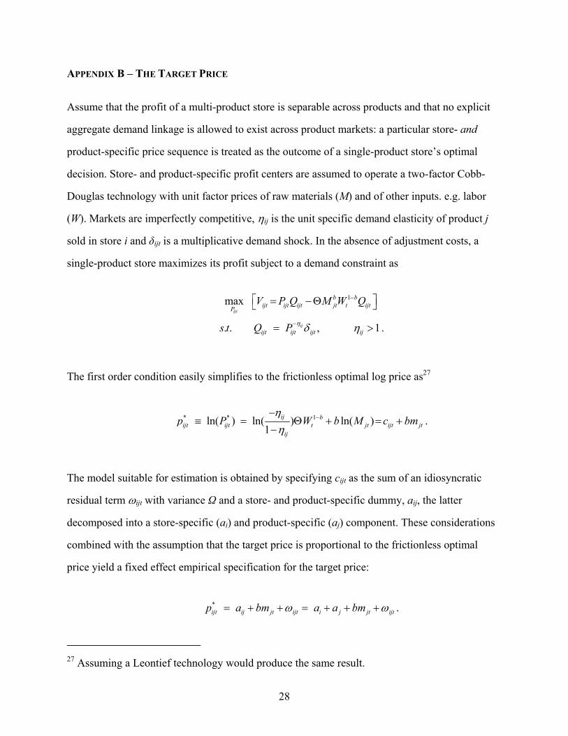
APPENDIX B – THE TARGET PRICE

Assume that the profit of a multi-product store is separable across products and that no explicit

aggregate demand linkage is allowed to exist across product markets: a particular store- and

product-specific price sequence is treated as the outcome of a single-product store’s optimal

decision. Store- and product-specific profit centers are assumed to operate a two-factor Cobb-

Douglas technology with unit factor prices of raw materials (M) and of other inputs. e.g. labor

(W). Markets are imperfectly competitive, ηij is the unit specific demand elasticity of product j

sold in store i and δijt is a multiplicative demand shock. In the absence of adjustment costs, a

single-product store maximizes its profit subject to a demand constraint as

1max

ijt

b bijt ijt ijt jt t ijtP

V P Q M W Q− = −Θ

. . , 1ijijt ijt ijt ijs t Q P η δ η−= > .

The first order condition easily simplifies to the frictionless optimal log price as27

* * 1ln( ) ln( ) ln( )

1ij b

ijt ijt t jt ijt jtij

p P W b M c bmηη

−−≡ = Θ + = +

−.

The model suitable for estimation is obtained by specifying cijt as the sum of an idiosyncratic

residual term ωijt with variance Ω and a store- and product-specific dummy, aij, the latter

decomposed into a store-specific (ai) and product-specific (aj) component. These considerations

combined with the assumption that the target price is proportional to the frictionless optimal

price yield a fixed effect empirical specification for the target price:

*ijt ij jt ijt i j jt ijtp a bm a a bmω ω= + + = + + + .

27 Assuming a Leontief technology would produce the same result.

29

References

Atkison, Andrew and Lee Ohanian (2001): Are Phillips Curves Useful for Forecasting Inflation?, Federal

Reserve Bank of Minneapolis Quarterly Review, pp. 2-11

Ball, Laurence and N. Gregory Mankiw (1994): Asymmetric Price Adjustment and Economic

Fluctuations, Economic Journal, pp. 247-261

Ball, Laurence and N. Gregory Mankiw (1995): Relative Price Changes as Aggregate Supply Shocks,

Quarterly Journal of Economics, pp. 161-193

Bertola, Giuseppe, Luigi Guiso and Luigi Pistaferri (2002): Uncertainty and Consumer Durables

Adjustment, manuscript

Bils, Mark and Peter J. Klenow (2002): Some Evidence on the Importance of Sticky Prices,

manuscript

Börsch-Supan, Axel and Hajivassiliou, Vassilis A. (1993): Smooth Unbiased Multivariate Probability

Simulators for Maximum Likelihood Estimation of Limited Dependent Variable Models, Journal

of Econometrics, pp. 347-368

Caballero, Ricardo J. and Eduardo M. R. A. Engel (1992): Price Rigidities, Asymmetries and Output

Fluctuations, NBER Working Paper #4091

Caballero, Ricardo J., Eduardo M. R. A. Engel and John C. Haltiwanger (1995): Plant Level Adjustment

and Aggregate Dynamics, Brookings Papers on Economic Activity, pp. 1-39

Caballero, Ricardo J., Eduardo M. R. A. Engel and John C. Haltiwanger (1997): Aggregate Employment

Dynamics: Building from Microeconomic Evidence, American Economic Review, pp. 115-137

Cecchetti, Stephen G. (1995): Inflation Indicators and Inflation Policy, NBER Macroeconomics Annual,

pp. 189-219

Cecchetti, Stephen G. and Erica L. Groshen (2000): Understanding Inflation: Implications for Monetary

Policy, NBER Working Paper #7482

Caplin, Andrew S. and John Leahy (1991): State-Dependent Pricing and the Dynamics of Money and

Output, Quarterly Journal of Economics, pp. 683-708

Dotsey, Michael, Robert G. King and Alexander L. Wolman (2000): State-Dependent Pricing and the

General Equilibrium Dynamics of Money and Output, Quarterly Journal of Economics, pp. 655-

690

Dunne, Timothy and Mark J. Roberts (1992): Costs, Demand, and Imperfect Competition as

Determinants of Plant-Level Output Prices, CES Working Paper, U.S. Bureau of the Census, 92-5

Eberly, Janice C. (1994): Adjustment in Consumers’ Durables Stocks: Evidence from Automobile

Purchases, Journal of Political Economy, pp. 403-437

30

Hajivassiliou, Vassilis A. and Daniel L. McFadden (1990): The Method of Simulated Scores for the

Estimation of LDV Models with an Application to External Debt Crises, manuscript

Heckman, James J. (1981a): Statistical Models for Discrete Panel Data, in C. Manski and D. McFadden

(eds.): Structural Analysis of Discrete Data with Econometric Applications, MTI Press, pp. 114-

177

Heckman, James J. (1981a): The Incidental Parameters Problem and the Problem of Initial Conditions in

Estimating a Discrete Time – Discrete Data Stochastic Process, in C. Manski and D. McFadden

(eds.): Structural Analysis of Discrete Data with Econometric Applications, MTI Press, pp. 179-

195

Keane, Michael P. (1993): Simulation Estimation for Panel Data Models with Limited Dependent

Variables, in Handbook of Statistics, Vol. 11, G. S. Maddala, C. R. Rao and H. D. Vinod (eds.),

Elsevier Science Publishers, pp. 545-571

Lach, Saul and Daniel Tsiddon (1992): The Behavior of Prices and Inflation: An Empirical Analysis of

Disaggregated Data, Journal of Political Economy, pp. 349-389

Lerman, S. and Charles Manski (1981): On the Use of Simulated Frequencies to Approximate Choice

Probabilities, in C. Manski and D. McFadden (eds.): Structural Analysis of Discrete Data with

Econometric Applications, MTI Press, pp. 305-319

Rátfai, Attila (2003): The Frequency and Size of Price Adjustment: Microeconomic Evidence,

Managerial and Decision Economics, forthcoming

Sheshinski, Eytan, Asher Tishler and Yoram Weiss (1981): Inflation, Costs of Adjustment, and the

Amplitude of Real Price Changes, in M. J. Flanders and A. Razin (eds.):,Developments in an

Inflationary World, Academic Press, pp. 195-207

Tsiddon, Daniel (1993): The (Mis)Behavior of the Aggregate Price Level, Review of Economic Studies,

pp. 889-902

Wolman, Alexander L. (2000): The Frequency and Costs of Individual Price Adjustment, Federal

Reserve Bank of Richmond, Economic Quarterly, pp. 1-22

Table 1Estimation Results

PERIOD 1 PERIOD 2

AR(0) AR(1) AR(0) AR(1)

sigma 0.216 0.161 0.155 0.120

(0.011) (0.009) (0.009) (0.007)

b 1.211 1.124 1.185 1.081

(0.025) (0.024) (0.043) (0.049)

S 0.349 0.248 0.213 0.151

(0.023) (0.02) (0.017) (0.015)

rho - 0.340 - 0.332

- (0.025) - (0.031)

lnL -87.930 -84.649 -89.729 -86.342

Notes: 1. Trinomial Probit panel regressions with actual nominal prices as dependent and raw material prices as explanatory variables.2. The AR(0) model is estimated by ML, the AR(1) by SML.3. sigma: standard deviation of residual, rho: autocerrelation parameter, b: slope parameter, s: lower adjusment boundary, lnL: mean log-likelihood.4. The lower adjustment boundary is fixed at s = -0.11.5. Estimations are carried out in Gauss. Standard errors are in parenthesis.

Table 2Partial Correlation

Π mm(z) stdev(z) skew(z)Π 1.000

mm(z) 0.352 1.000stdev(z) 0.219 -0.106 1.000skew(z) 0.336 0.689 0.036 1.000

Note: Π denotes inflation, stdev(z) denotes standard deviation, skew(z) denotes skewness, mm(z) denotes the mean-median difference in price deviation densities.

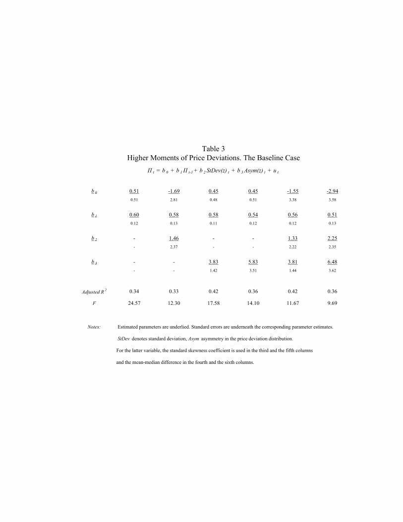
Table 3Higher Moments of Price Deviations. The Baseline Case

Π t = b 0 + b 1Π t-1 + b 2 StDev(z) t + b 3 Asym(z) t + u t

b 0 0.51 -1.69 0.45 0.45 -1.55 -2.940.51 2.81 0.48 0.51 3.38 3.58

b 1 0.60 0.58 0.58 0.54 0.56 0.510.12 0.13 0.11 0.12 0.12 0.13

b 2 - 1.46 - - 1.33 2.25- 2.37 - - 2.22 2.35

b 3 - - 3.83 5.83 3.81 6.48- - 1.42 3.51 1.44 3.62

Adjusted R 2 0.34 0.33 0.42 0.36 0.42 0.36

F 24.57 12.30 17.58 14.10 11.67 9.69

Notes: Estimated parameters are underlied. Standard errors are underneath the corresponding parameter estimates.

StDev denotes standard deviation, Asym asymmetry in the price deviation distribution.

For the latter variable, the standard skewness coefficient is used in the third and the fifth columns

and the mean-median difference in the fourth and the sixth columns.

Table 4Counterfactual Inflation with Time Variation in f(.) and A(.) Suppressed

G(.) A(oa) A(s) A(a)

f(oa) 0.00 0.32 0.37

f(s) 0.50 0.69 0.74

f(a) 0.79 0.90 1.00

Note: a denotes actual, s seasonal average, oa overall average

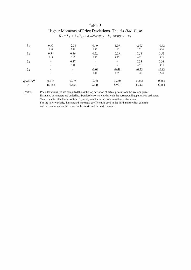
Table 5Higher Moments of Price Deviations. The Ad Hoc Case

Π t = b 0 + b 1Π t-1 + b 2 StDev(x) t + b 3 Asym(x) t + u t

b 0 0.37 -2.36 0.49 1.59 -2.05 -0.420.38 2.58 0.43 5.93 2.73 6.20

b 1 0.54 0.56 0.52 0.53 0.54 0.550.13 0.13 0.13 0.13 0.13 0.13

b 2 - 0.37 - - 0.33 0.38- 0.34 - - 0.35 0.35

b 3 - - -0.09 -0.49 -0.55 -0.83- - 0.14 2.39 1.40 2.40

Adjusted R 2 0.276 0.278 0.266 0.260 0.262 0.263F 18.155 9.684 9.148 8.901 6.313 6.364

Notes: Price deviations (x ) are computed the as the log deviation of actual prices from the average price.Estimated parameters are underlied. Standard errors are underneath the corresponding parameter estimates.StDev denotes standard deviation, Asym asymmetry in the price deviation distribution. For the latter variable, the standard skewness coefficient is used in the third and the fifth columnsand the mean-median difference in the fourth and the sixth columns.

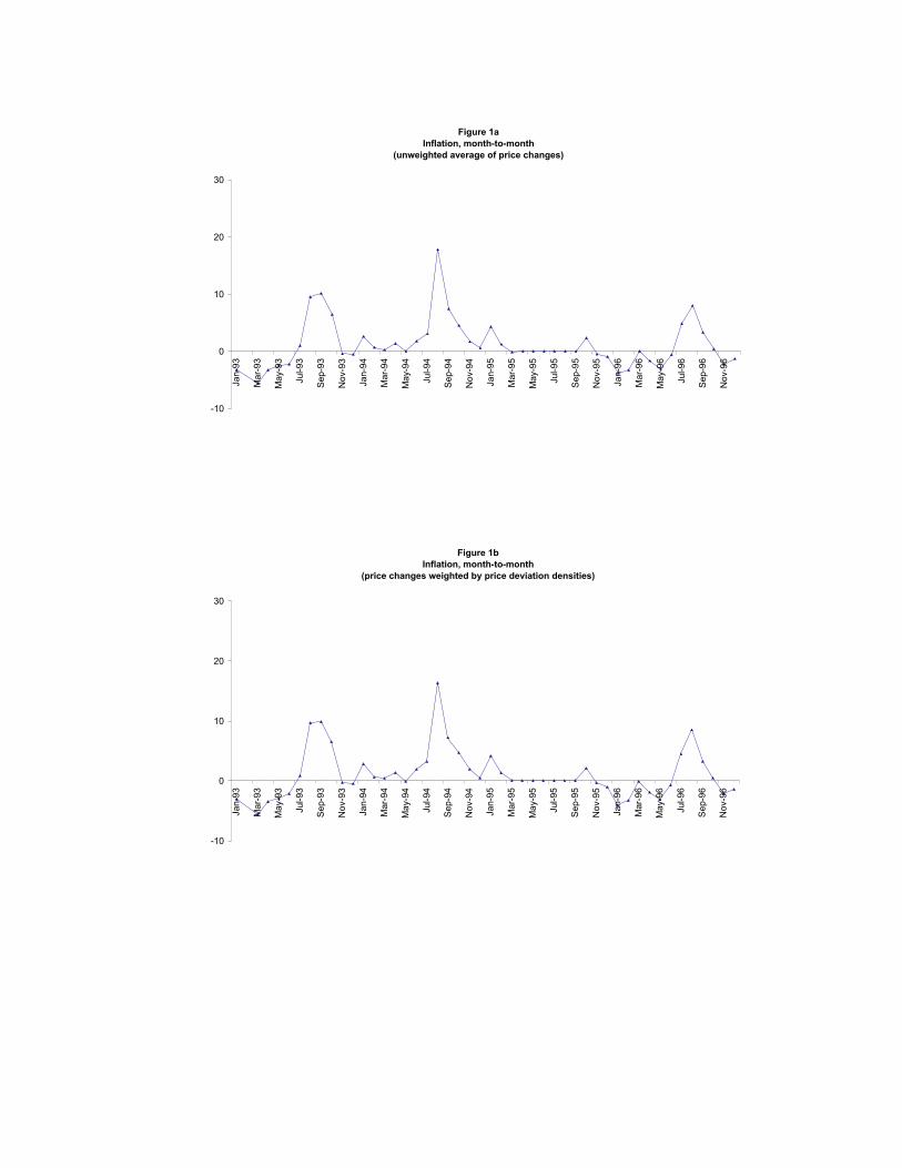
Figure 1aInflation, month-to-month

(unweighted average of price changes)

-10

0

10

20

30

Jan-93

Mar-93

May-93

Jul-93

Sep-93

Nov-93

Jan-94

Mar-94

May-94

Jul-94

Sep-94

Nov-94

Jan-95

Mar-95

May-95

Jul-95

Sep-95

Nov-95

Jan-96

Mar-96

May-96

Jul-96

Sep-96

Nov-96

Figure 1bInflation, month-to-month

(price changes weighted by price deviation densities)

-10

0

10

20

30

Jan-93

Mar-93

May-93

Jul-93

Sep-93

Nov-93

Jan-94

Mar-94

May-94

Jul-94

Sep-94

Nov-94

Jan-95

Mar-95

May-95

Jul-95

Sep-95

Nov-95

Jan-96

Mar-96

May-96

Jul-96

Sep-96

Nov-96

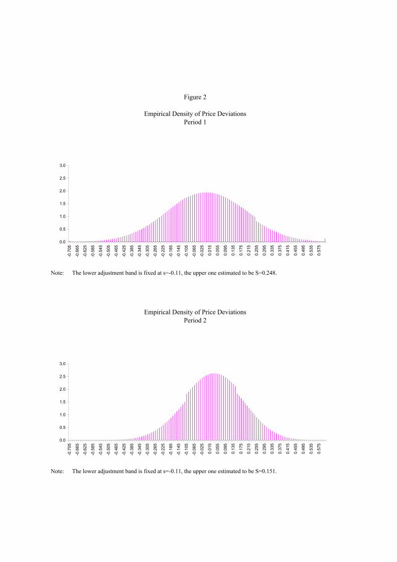
Note: The lower adjustment band is fixed at s=-0.11, the upper one estimated to be S=0.248.

Note: The lower adjustment band is fixed at s=-0.11, the upper one estimated to be S=0.151.

Figure 2

Empirical Density of Price DeviationsPeriod 1

0.0

0.5

1.0

1.5

2.0

2.5

3.0

-0.705

-0.665

-0.625

-0.585

-0.545

-0.505

-0.465

-0.425

-0.385

-0.345

-0.305

-0.265

-0.225

-0.185

-0.145

-0.105

-0.065

-0.025

0.015

0.055

0.095

0.135

0.175

0.215

0.255

0.295

0.335

0.375

0.415

0.455

0.495

0.535

0.575

Empirical Density of Price DeviationsPeriod 2

0.0

0.5

1.0

1.5

2.0

2.5

3.0

-0.705

-0.665

-0.625

-0.585

-0.545

-0.505

-0.465

-0.425

-0.385

-0.345

-0.305

-0.265

-0.225

-0.185

-0.145

-0.105

-0.065

-0.025

0.015

0.055

0.095

0.135

0.175

0.215

0.255

0.295

0.335

0.375

0.415

0.455

0.495

0.535

0.575

Figure 3Empirical Densities of Price Deviations - Quarterly

1993 1994 1995 1996Q1 Q5 Q9 Q13

Q2 Q6 Q10 Q14

Q3 Q7 Q11 Q15

Q4 Q8 Q12 Q16

NotesThe solid lines are third degree polynomials fitted to the empirical densities.Data from Q10 and Q11 are missing. The lower adjustment bands are fixed at s=-0.11.

01234

-0.705

-0.535

-0.365

-0.195

-0.025

0.145

0.315

0.485

01234

-0.705

-0.535

-0.365

-0.195

-0.025

0.145

0.315

0.485

0

1234

-0.705

-0.535

-0.365

-0.195

-0.025

0.145

0.315

0.485

01234

-0.705

-0.535

-0.365

-0.195

-0.025

0.145

0.315

0.485

01234

-0.705

-0.535

-0.365

-0.195

-0.025

0.145

0.315

0.485

01234

-0.705

-0.555

-0.405

-0.255

-0.105

0.045

0.195

0.345

0.495

01234

-0.705

-0.555

-0.405

-0.255

-0.105

0.045

0.195

0.345

0.495

01234

-0.705

-0.555

-0.405

-0.255

-0.105

0.045

0.195

0.345

0.495

01234

-0.705

-0.555

-0.405

-0.255

-0.105

0.045

0.195

0.345

0.495

01234

-0.705

-0.555

-0.405

-0.255

-0.105

0.045

0.195

0.345

0.495

0

1234

-0.705

-0.555

-0.405

-0.255

-0.105

0.045

0.195

0.345

0.495

01234

-0.705

-0.555

-0.405

-0.255

-0.105

0.045

0.195

0.345

0.495

01234

-0.705

-0.555

-0.405

-0.255

-0.105

0.045

0.195

0.345

0.495

01234

-0.705

-0.555

-0.405

-0.255

-0.105

0.045

0.195

0.345

0.495

Note: The lower adjustment band is fixed at s=-0.11, the upper one estimated to be S=0.248.

Note: The lower adjustment band is fixed at s=-0.11, the upper one estimated to be S=0.151.

Figure 4

Adjustment FunctionPeriod 1

-60

-50

-40

-30

-20

-10

0

-0.705

-0.665

-0.625

-0.585

-0.545

-0.505

-0.465

-0.425

-0.385

-0.345

-0.305

-0.265

-0.225

-0.185

-0.145

-0.105

-0.065

-0.025

0.015

0.055

0.095

0.135

0.175

0.215

0.255

0.295

0.335

0.375

0.415

0.455

0.495

0.535

0.575

Adjustment FunctionPeriod 2

-60

-50

-40

-30

-20

-10

0

-0.705

-0.665

-0.625

-0.585

-0.545

-0.505

-0.465

-0.425

-0.385

-0.345

-0.305

-0.265

-0.225

-0.185

-0.145

-0.105

-0.065

-0.025

0.015

0.055

0.095

0.135

0.175

0.215

0.255

0.295

0.335

0.375

0.415

0.455

0.495

0.535

0.575

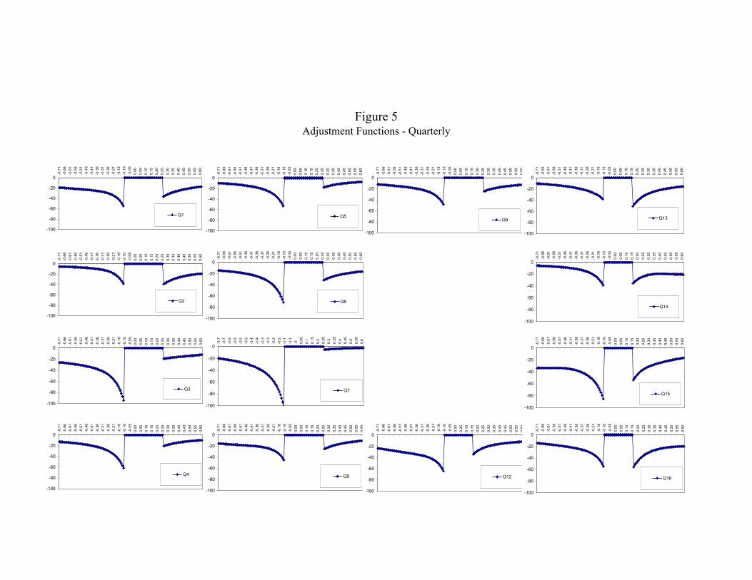
Figure 5Adjustment Functions - Quarterly

-100

-80

-60

-40

-20

0

-0.71

-0.66

-0.61

-0.56

-0.51

-0.46

-0.41

-0.36

-0.31

-0.26

-0.21

-0.16

-0.10

-0.05

0.00

0.05

0.10

0.15

0.20

0.25

0.30

0.35

0.40

0.45

0.50

0.55

0.60

Q1

-100

-80

-60

-40

-20

0

-0.71

-0.66

-0.61

-0.56

-0.51

-0.46

-0.41

-0.36

-0.31

-0.26

-0.21

-0.16

-0.10

-0.05

0.00

0.05

0.10

0.15

0.20

0.25

0.30

0.35

0.40

0.45

0.50

0.55

0.60

Q2

-100

-80

-60

-40

-20

0

-0.71

-0.66

-0.61

-0.56

-0.51

-0.46

-0.41

-0.36

-0.31

-0.26

-0.21

-0.16

-0.10

-0.05

0.00

0.05

0.10

0.15

0.20

0.25

0.30

0.35

0.40

0.45

0.50

0.55

0.60

Q3

-100

-80

-60

-40

-20

0

-0.71

-0.66

-0.61

-0.56

-0.51

-0.46

-0.41

-0.36

-0.31

-0.26

-0.21

-0.16

-0.10

-0.05

0.00

0.05

0.10

0.15

0.20

0.25

0.30

0.35

0.40

0.45

0.50

0.55

0.60

Q4

-100

-80

-60

-40

-20

0

-0.71

-0.66

-0.61

-0.56

-0.51

-0.46

-0.41

-0.36

-0.31

-0.26

-0.21

-0.16

-0.10

-0.05

0.00

0.05

0.10

0.15

0.20

0.25

0.30

0.35

0.40

0.45

0.50

0.55

0.60

Q5

-100

-80

-60

-40

-20

0

-0.71

-0.66

-0.61

-0.56

-0.51

-0.46

-0.41

-0.36

-0.31

-0.26

-0.21

-0.16

-0.10

-0.05

0.00

0.05

0.10

0.15

0.20

0.25

0.30

0.35

0.40

0.45

0.50

0.55

0.60

Q6

-100

-80

-60

-40

-20

0

-0.7

-0.7

-0.6

-0.6

-0.5

-0.5

-0.4

-0.4

-0.3

-0.3

-0.2

-0.2

-0.1

-0.1

-0 0.05

0.1

0.15

0.2

0.25

0.3

0.35

0.4

0.45

0.5

0.55

0.6

Q7

-100

-80

-60

-40

-20

0

-0.71

-0.66

-0.61

-0.56

-0.51

-0.46

-0.41

-0.36

-0.31

-0.26

-0.21

-0.16

-0.10

-0.05

0.00

0.05

0.10

0.15

0.20

0.25

0.30

0.35

0.40

0.45

0.50

0.55

0.60

Q8

-100

-80

-60

-40

-20

0

-0.71

-0.66

-0.61

-0.56

-0.51

-0.46

-0.41

-0.36

-0.31

-0.26

-0.21

-0.16

-0.10

-0.05

0.00

0.05

0.10

0.15

0.20

0.25

0.30

0.35

0.40

0.45

0.50

0.55

0.60

Q9

-100

-80

-60

-40

-20

0

-0.71

-0.66

-0.61

-0.56

-0.51

-0.46

-0.41

-0.36

-0.31

-0.26

-0.21

-0.16

-0.10

-0.05

0.00

0.05

0.10

0.15

0.20

0.25

0.30

0.35

0.40

0.45

0.50

0.55

0.60

Q12

-100

-80

-60

-40

-20

0

-0.71

-0.66

-0.61

-0.56

-0.51

-0.46

-0.41

-0.36

-0.31

-0.26

-0.21

-0.16

-0.10

-0.05

0.00

0.05

0.10

0.15

0.20

0.25

0.30

0.35

0.40

0.45

0.50

0.55

0.60

Q13

-100

-80

-60

-40

-20

0

-0.71

-0.66

-0.61

-0.56

-0.51

-0.46

-0.41

-0.36

-0.31

-0.26

-0.21

-0.16

-0.10

-0.05

0.00

0.05

0.10

0.15

0.20

0.25

0.30

0.35

0.40

0.45

0.50

0.55

0.60

Q14

-100

-80

-60

-40

-20

0

-0.71

-0.66

-0.61

-0.56

-0.51

-0.46

-0.41

-0.36

-0.31

-0.26

-0.21

-0.16

-0.10

-0.05

0.00

0.05

0.10

0.15

0.20

0.25

0.30

0.35

0.40

0.45

0.50

0.55

0.60

Q15

-100

-80

-60

-40

-20

0

-0.71

-0.66

-0.61

-0.56

-0.51

-0.46

-0.41

-0.36

-0.31

-0.26

-0.21

-0.16

-0.10

-0.05

0.00

0.05

0.10

0.15

0.20

0.25

0.30

0.35

0.40

0.45

0.50

0.55

0.60

Q16

Dispersion, Asymmetry and Aggregate Inflation

Notes: Inflation, month-to-month (DP-m) is measured on the left axes, other variables on the right ones. "stdev(z)" and "skew(z)" denote the standard deviation and the skewness of the distribution of price deviations, respectively. "mm(z)" denotes the mean-median difference in the distribution of price deviations.

Figure 6

-6-30369121518

Jan-93

May-93

Aug-93

Nov-93

Feb-94

May-94

Aug-94

Nov-94

Feb-95

May-95

Aug-95

Nov-95

Feb-96

May-96

Aug-96

Nov-96

0.10

0.12

0.14

0.16

0.18

0.20

DP-mStDev(z)

-6-30369121518

Jan-93

May-93

Aug-93

Nov-93

Feb-94

May-94

Aug-94

Nov-94

Feb-95

May-95

Aug-95

Nov-95

Feb-96

May-96

Aug-96

Nov-96

-1.0

-0.6

-0.2

0.2

0.6

1.0

DP-mSkew(z)

-6-30369121518

Jan-93

May-93

Aug-93

Nov-93

Feb-94

May-94

Aug-94

Nov-94

Feb-95

May-95

Aug-95

Nov-95

Feb-96

May-96

Aug-96

Nov-96

-0.03-0.02-0.010.000.010.020.030.04

DP-mmm(z)

Figure 7True vs. Counterfactual Aggregate Inflation

Note : The dashed line is the true aggregate inflation series, the solid line is the counterfactual one. The counterfactual is constructed by replacing the

benchmark cross-sectional density of price deviations with the one computed by suppressing idiosyncratic shocks.

-10

-5

0

5

10

15

20

Jan-93

May-93

Aug-93

Nov-93

Feb-94

May-94

Aug-94

Nov-94

Feb-95

May-95

Aug-95

Nov-95

Feb-96

May-96

Aug-96

Nov-96

Figure 8

Empirical Density of Price Deviations - Full Sample, Idiosyncratic shocks suppressed

0.0

0.5

1.0

1.5

2.0

2.5

3.0

3.5

4.0

4.5

5.0

-0.705

-0.675

-0.645

-0.615

-0.585

-0.555

-0.525

-0.495

-0.465

-0.435

-0.405

-0.375

-0.345

-0.315

-0.285

-0.255

-0.225

-0.195

-0.165

-0.135

-0.105

-0.075

-0.045

-0.015

0.015

0.045

0.075

0.105

0.135

0.165

0.195

0.225

0.255

0.285

0.315

0.345

0.375

0.405

0.435

0.465

0.495

0.525

0.555

0.585