From Aggregate Betting Data

to Individual Risk Preferences∗

Pierre-Andre Chiappori† Bernard Salanie‡ Francois Salanie§

Amit Gandhi¶

May 4, 2017

Abstract

We show that even in the absence of data on individual decisions, the distribution

of individual attitudes towards risk can be identified from the aggregate conditions that

characterize equilibrium on markets for risky assets. Taking horse races as a textbook

model of contingent markets, we allow for heterogeneous bettors with very general risk

preferences, including non-expected utility. Under a standard single-crossing condition

on preferences, testable implications can be derived, and parimutuel data allow us to

uniquely identify the distribution of preferences among the population of bettors. We

estimate the model on data from US races. Specifications based on expected utility fit

the data very poorly. Our results stress the crucial importance of nonlinear probability

weighting. They also suggest that several dimensions of heterogeneity may be at work.

∗This paper was first circulated and presented under the title “What you are is what you bet: elicitingrisk attitudes from horse races.” We thank the editor, four referees, and many seminar audiences for theircomments. We are especially grateful to Jeffrey Racine for advice on nonparametric and semiparametricapproaches, and to Simon Wood for help with his R package mgcv. Bernard Salanie received financialsupport from the European Research Council under the European Community’s Seventh Framework ProgramFP7/2007-2013 grant agreement No. 295298. Pierre-Andre Chiappori gratefully acknowledges financialsupport from NSF (Award 1124277.)†Columbia University. Email: pc2167@columbia.edu‡Columbia University. Email: bsalanie@columbia.edu§Toulouse School of Economics, University of Toulouse Capitole, INRA, Toulouse, France. Email: fran-

cois.salanie@inra.fr¶University of Wisconsin-Madison. Email: agandhi@ssc.wisc.edu

1

Introduction

The literature devoted to the empirical estimation of individual attitudes to risk is by now

quite large1 To quote but a few recent examples, Barsky et al. (1997) use survey questions

and observations of actual behavior to measure relative risk aversion. Results indicate that

this parameter varies between 2 (for the first decile) and 25 (for the last decile), and that

this heterogeneity is poorly explained by demographic variables. Guiso and Paiella (2006)

report similar findings, and use the term “massive unexplained heterogeneity”. Chiappori

and Paiella (2011) observe the financial choices of a sample of households across time, and use

these panel data to show that while a model with constant relative risk aversion well explains

each household’s choices, the corresponding coefficient is highly variable across households

(its mean is 4.2, for a median of 1.7.) Distributions of risk aversions have also been estimated

using data on television games (Beetsma and Schotman, 2001), insurance markets (Cohen

and Einav, 2007; Barseghyan et al., 2013, 2016) or risk sharing within closed communities

(Bonhomme et al., 2012; Chiappori et al. 2012).

These papers and many others all rely on data on individual behavior. Indeed, a widely

shared view posits that microdata are indispensable to analyze attitudes to risk, particularly

in the presence of observed or unobserved heterogeneity. The present paper challenges this

claim. It argues that, in many contexts, the distribution of risk attitudes can be nonpara-

metrically identified, even in the absence of data on individual decisions; we only need to use

the aggregate conditions that characterize an equilibrium, provided that these equilibria can

be observed on a large set of different “markets”. While a related approach has often been

used in other fields (e.g., empirical industrial organization), to the best of our knowledge,

it has never been applied to the estimation of a distribution of individual attitudes towards

risk.

The main intuition underlying our approach can be summarized as follows. In any

model that involves equilibrium under uncertainty, the relationship between the payoffs of

risky choices and the equilibrium prices plays a crucial role. In financial economics for

instance, the risky payoffs are the asset returns, and this relationship is summed up in

a pricing kernel. If all agents are risk neutral, then the relationship between prices and

stochastic processes is very simple: the price of an asset exclusively reflects the expected

value of its returns. No higher-order moment is relevant; neither is the distribution of the

1Among earlier attempts to measure the dispersion of risk aversion, one may mention for instance Bin-swanger (1980), Hey and Orme (1994), and the references in Wik et al. (2004). We thank an anonymousreferee for suggesting some of these references.

2

returns of other assets. Any deviation from the risk neutrality benchmark leads to a more

complex relationship, especially if it allows for heterogeneous attitudes towards risk among

investors. The crux of our argument is that one can reverse-engineer this relationship: the

observed mapping between stochastic processes and equilibrium prices reveals information

about the distribution of risk attitudes within the population under consideration. Our first

contribution is to show that one may not need to observe individual choices: knowing the

pricing kernel may be sufficient.

In practice, applying this general strategy to financial markets raises several challenging

difficulties. For instance, a crucial problem is the nature of the individual decision under

scrutiny: portfolio choice is a complex problem, requiring multidimensional optimization on

continuous variables. In addition, the exact nature of the stochastic processes involved is

also very complex, and it is fair to say that there are diverging views about the best ways

to model them. Finally, financial decisions involve dynamic issues that are far from obvious.

While ultimately modeling such phenomena remains on our research agenda, we start in this

paper with a much simpler context. We focus on “win bets” placed in horse races that use

parimutuel betting. Bettors choose which horse to bet on, and those who bet on the winning

horse share the total amount wagered in the race (minus the organizer’s take.) This has

several attractive properties for our purposes. First, a win bet is simply a state-contingent

asset. Second, observing the odds of a horse—the rate of return if it wins—is equivalent to

observing its market share. Large samples of races are readily available. Finally, the decision

we model is essentially discrete (which horse to bet on), and the nature of the stochastic

process is very simple.

In such horse bets, the intuition described above has a very simple translation. For any

given race, we can simultaneously observe or at least recover both the odds and the winning

probability of each horse. In the risk neutral benchmark, odds would be directly proportional

to winning probabilities. In general, the variation in odds (or market shares) from race to

race as a function of winning probabilities conveys information on how bettors react to given

lotteries. If we observe a large enough number of races with enough variation in odds and

winning probabilities, then under the assumption that the population of bettors has the

same distribution of preferences in all races we can learn its characteristics by observing the

mapping from race odds to probabilities.

We analyze two sets of questions. The first one is testability: can one derive, from some

general, theoretical representation of individual decision under uncertainty, testable restric-

tions on equilibrium patterns—as summarized by the relationship between probabilities and

3

odds? The second issue relates to identifiability: under which conditions is it possible to

recover, from the same equilibrium patterns, the structure of the underlying model—i.e., the

distribution of individual preferences? In both cases, our goal is to minimize the restrictions

we a priori impose on the distribution of preferences. A large fraction of the related lit-

erature assumes homogeneous preferences, expected utility maximization, or both; at best,

estimates of heterogeneous distributions or non-expected utility specifications rely on a very

strict parametrization of both preferences and unobserved heterogeneity. On the contrary,

our aim is to remain very flexible on two dimensions.

While additional restrictions are obviously necessary to reach this goal, we show that

they are surprisingly mild. Essentially, three assumptions are needed. One is that, when

choosing between lotteries, agents only consider their direct outcomes: the utility derived

from choosing one of them (here, betting on a horse with a given winning probability) does

not depend on the characteristics of the others. While this assumption does rule out a few

existing frameworks (e.g., those based on regret theory), it remains compatible with the

vast majority of models of decision-making under uncertainty. Secondly, we assume that

agents’ decisions regarding bets are based on the true distribution of winning probabilities.

An assumption of this kind is indispensable in our context, as any observed pattern can be

rationalized by a well chosen distribution of individual beliefs. Note however that we do

not assume that valuations are linear in probabilities; on the contrary, we allow for the type

of probability weighting emphasized by modern decision theory, starting with Yaari’s dual

model or Kahneman and Tversky’s cumulative prospect theory. Finally, we assume that

heterogeneity of preferences is one-dimensional, and satisfies a standard single-crossing con-

dition. Note that the corresponding heterogeneity may affect utility, probability weighting,

or both; in that sense, our framework is compatible with a wide range of theoretical under-

pinnings. Also, our methods can be extended to at least some forms of multi-dimensional

heterogeneity; while we address this briefly, we leave a more general treatment for future

research.

Our main theoretical result states that, under these three conditions, an equilibrium

always exists, is unique, and that the answer to both previous questions is positive. We derive

strong testable restrictions on equilibrium patterns. When these restrictions are fulfilled, we

can identify the distribution of preferences in the population of bettors; in particular, we

can compare various classes of preferences and distributions.

We then provide an empirical application of these results. In our setting, the concept of

normalized fear of ruin (NF) provides the most adequate representation of the risk/return

4

trade off. Normalized fear of ruin directly generalizes the fear of ruin index introduced in an

expected utility setting by Aumann and Kurz (1977). Bettors value returns (odds) as well

as the probability of winning. The NF simply measures the elasticity of required return with

respect to probability along an indifference curve in this space. As such, it can be defined

under expected utility maximization, in which case it does not depend on probabilities; but

also in more general frameworks, with probability weightings or various non-separabilities.

We show that the identification problem boils down to recovering the NF index as a function

of odds, probabilities and a one-dimensional heterogeneity parameter. We provide a set of

necessary and sufficient conditions for a given function to be an NF; these provide the testable

restrictions mentioned above. We also show that under these conditions, the distribution of

NF is non parametrically identified. In addition, we extend these results to the case when

bettors decide which races they will bet on. For reasons discussed below, we do not explicitly

consider that decision in our empirical exercise.

Finally, we estimate our model on a sample of more than 25,000 races involving some

200,000 horses. Since the populations in the various “markets” must, in our approach,

have similar distributions of preferences, we focus on races taking place during weekdays,

on urban racetracks. Since we observe market shares, the single-crossing assumption allows

us to characterize the one-dimensional index of each marginal bettor (i.e., the rank of the

bettor indifferent between two horses). We specify a very general value function that depends

on the winning probability, the corresponding return, and this index, based on orthogonal

polynomials. We use the indifference conditions to estimate the winning probabilities and

parameters by a simple log-likelihood maximization. The advantage of such a strategy is that

it allows for non parametric estimation of both a general model (involving unrestricted non

expected utility with general one-dimensional heterogeneity) and several nested submodels

(including homogeneous and heterogenous versions of expected utility maximization, Yaari’s

dual model and rank-dependent expected utility).

Our empirical conclusions are quite striking. First, the type of preferences that are

routinely used in the applied literature (e.g., constant relative or absolute risk aversion)

are incompatible with the data. They imply restrictive conditions on the shape of the NF

functions that our estimates clearly reject.2 This suggests that the parametric approaches

adopted in much applied work should be handled with care, at least when applied to the

type of data considered here, as they may imply unduly restrictive assumptions.

2For instance, under such commonly used representations as CARA or CRRA preferences, any givenindividual is either always risk-averse or always risk-loving. However, under our preferred specification agiven bettor may be risk averse for some bets and risk loving for others.

5

Secondly, models relying on an expected utility (EU) framework do not perform well;

their fit is quite poor, even for heterogeneous versions of the model. Moreover, single-

crossing restrictions are violated for approximately half of our sample, thus casting a doubt

on whether a one-dimensional index is enough to capture the impact of heterogeneity. In fact,

our preferred models are relatively parsimonious versions of homogeneous rank-dependent

expected utility (RDEU) preferences, and of homogeneous NEU preferences. In both cases,

the main role is played by distortions of probabilities.3 Introducing heterogeneity within

the NEU framework further improves the fit, but only slightly; this last conclusion must be

taken with a pinch of salt, since we may be reaching the limits of what our data can robustly

say.

Related Literature

The notion that testable restrictions may be generated regarding the form of the equi-

librium manifold is not new, and can be traced back to Brown and Matzkin (1996) and

Chiappori et al. (2002, 2004); the latter, in addition, introduce the idea of recovering in-

dividual preferences from the structure of the manifold. But to the best of our knowledge,

these papers have not led to empirical applications. Our contributions here are most closely

related to the literature on estimating and evaluating theories of individual risk preferences,

and also to the literature on identification of random utility models. There is now a large

literature that tests and measures theories of individual risk preference using laboratory

methods (see e.g. Camerer and Kunreuther, 1989; Harless and Camerer, 1994; and Bruhin

et al., 2010). There is also a sizable literature that directly elicits individual risk preferences

through survey questions (see e.g., Barsky et al., 1997; Bonin et al., 2007; Dohmen et al.,

2011) and correlates these measures with other economic behaviors. The literature that

studies risk preferences as revealed by market transactions is much more limited. Most of

it has focused on insurance choices (see e.g., Cohen and Einav, 2007; Sydnor, 2010; and

Barseghyan et al., 2013 and 2016) and gambling behavior (see e.g., Andrikogiannopoulou

and Papakonstantinou, 2016). However all of these studies fundamentally exploit individual

level demand data to estimate risk preferences and document heterogeneity.

The literature on estimating risk preferences from market level data has almost exclu-

sively used a representative agent paradigm. Starting with Weitzman (1965), betting markets

have served as a natural source of data for representative agent studies of risk preferences

3See Barberis (2013) for a recent analysis of probability weighting,

6

due to the textbook nature of the gambles that are offered. In the context of racetrack bet-

ting, Jullien and Salanie (2000) and Snowberg and Wolfers (2010) provide evidence showing

that a representative agent with non-linear probability weighting better explains the pat-

tern of prices at the racetrack as compared to an expected utility maximizing representative

agent. Aruoba and Kearney (2011) present similar findings using cross sectional prices and

quantities from state lotteries. These representative agent studies of betting markets stand

in contrast to a strand of research that has emphasized belief heterogeneity as an impor-

tant determinant of equilibrium in security markets. Ottaviani and Sorensen (2010) and

Gandhi and Serrano-Padial (2014) argue that heterogeneity of beliefs and/or information

of risk neutral agents can explain the well-known favorite-longshot bias that characterizes

many betting markets. Gandhi and Serrano-Padial furthermore estimate the degree of belief

heterogeneity revealed by equilibrium patterns. In contrast, our aim here is to fully explore

the consequences of heterogeneity in preferences. Our paper is the only one to date that

nonparametrically identifies and estimates heterogeneous risk preferences from market level

data. Furthermore, while our theoretical framework excludes heterogeneity in beliefs, it

allows for heterogeneity in probability weighting across agents; and our nonparametric ap-

proach allows us to compare this and other theories (such as heterogeneity in risk preferences

in an expected utility framework.)

Finally, our paper makes a contribution to the identification of random utility models of

demand. Random utility models have become a popular way to model market demand for

differentiated products following Bresnahan (1987), Berry (1994), and Berry et al. (1995).

A lingering question in this literature is whether preference heterogeneity can indeed be

identified from market level observations alone. Along with Chiappori, Gandhi, Salanie

and Salanie (2009), our paper shows that a non-parametric model of vertically differen-

tiated demand can be identified from standard variation in the set of products available

across markets. In particular we exploit a one dimensional source of preference heterogene-

ity that satisfies a standard single crossing condition consistent with vertically differentiated

demand. We show that the identification of inverse demand from the data allows us to

non-parametrically recover this class of preferences. This stands in contrast to the work

by Berry and Haile (2016), who use full-support variation in a “special regressor” to show

that an arbitrary random utility model can be recovered from inverse demand4. We instead

show identification of random utility without a special regressor by exploiting the additional

4See also Gautier and Kitamura (2013) on the binary choice model and Kitamura and Stoye (2016) forthe Random Utility Model.

7

restriction that random utility satisfies the single crossing structure.

We present the institution, assumptions, and the structure of market equilibrium in sec-

tion 1. In section 2, we explain the testable restrictions on observed demand behavior implied

by the model, and we show that these restrictions are sufficient to identify preferences. Sec-

tion 3 describes the data, while Section 4 discusses the estimation strategy. We describe our

results in Section 5, and we end with some concluding remarks. Appendix A gathers the

proofs of our results, while Appendix B details our estimation results.

1 Theoretical framework

Parimutuel We start with the institutional organization of parimutuel betting. Consider

a race with horses i = 1, . . . , n. We focus on “win bets”, i.e. bets on the winning horse: each

dollar bet on horse i pays a net return of Ri dollars if horse i wins, and is lost otherwise. Ri

is called the odds of horse i, and in parimutuel races it is determined by the following rule:

all money wagered by bettors constitutes a pool that is redistributed to those who bet on the

winning horse, apart from a share t corresponding to taxes and a “house take”. Accordingly,

if si is the share of the pool corresponding to the sums wagered on horse i, the payment to

a winning bet of $1 is

Ri + 1 =1− tsi

(1)

Hence odds are not set by bookmakers; instead they are determined by the distribution (s1,

. . . , sn) of bets among horses. Odds are mechanically low for those horses on which many

bettors laid money (favorites), and they are high for longshots5. Since market shares sum to

one, these equations together imply

1

1− t=∑i

1

Ri + 1(2)

Hence knowing the odds (R1, . . . , Rn) allows to compute both the take t and the shares in

the pool (s1, . . . , sn).

5According to this formula odds can even be negative, if si is above (1− t); it never happens in our data.

8

Probabilities We now define a n-horse race (p, t) by a vector of positive probabilities p =

(p1, . . . , pn) in the n-dimensional simplex, and a take t ∈ (0, 1). Note that pi is the objective

probability that horse i wins the race. Our setting is thus compatible with traditional models

of decision under uncertainty, in which all agents agree on the probabilities of the various

states of the world, and these probabilities are correct. This framework singles out preferences

as the driving determinant of odds; it accords well with empirical work that shows how odds

reflect most relevant information about winning probabilities6. It is also consistent with the

familiar rational expectations hypothesis; in fact, we will show that a rational expectations

equilibrium exists and is unique in our setting. It is important to stress, however, that our

framework is also compatible with more general models of decision-making. In particular,

it allows for the type of probability weighting that characterizes many non-expected utility

functionals, whereby the actual decision process may involve arbitrary increasing functions

of the probabilities. Moreover, these probability weights may be agent-specific, as we shall

see. In other words, our general framework encompasses both “traditional” models, in which

agents always refer to objective probability and heterogeneity only affects preferences, and

more general versions in which different agents weigh probabilities differently. The only

strong restriction we will impose bears on the dimension of the heterogeneity, not on its

nature.

Following the literature to date7, we endow each bettor with a standardized bet amount

that he allocates to his most preferred horse in the race. In particular, we do not allow

participants to bet heterogeneous amounts. Therefore the shares (si) in the pool defined

above can be identified to market shares. Any bettor looks on a bet on horse i as a lottery

that pays returns Ri with probability pi, and pays returns (−1) with probability (1−pi). We

denote this lottery by (Ri, pi), and call it a gamble. By convention, throughout the paper we

index horses by decreasing probabilities (p1 > · · · > pn > 0), so that horse 1 is the favorite.

Risk neutral bettors As a benchmark, consider the case when bettors are risk-neutral,

and thus only consider the expected gain associated to any specific bet8. Equilibrium then

6See Sung and Johnson (2008) and Ziemba (2008) for recent surveys on the informational efficiency ofbetting markets.

7See Weitzman (1965), Jullien and Salanie (2000), Snowberg and Wolfers (2010), among others.8Clearly, a risk neutral player will not take a bet with a negative expected value unless she derives some

fixed utility from gambling. The assumption we maintain in this paper is that the “utility of gambling”(Conlisk, 1993) which explains why such people gamble to start with does not depend on the particularhorse on which the bet is placed: conditional on betting, bettors still select the horse that generates thehighest expected gain.

9

requires expected values to be equalized across horses. Since bets (net of the take) are

redistributed, this yields:

piRi − (1− pi) = −t

which, together with (2), gives probabilities equal to

pni (R1, . . . , Rn) =

1

Ri + 1∑j

1

Rj + 1

=1− t

1 +Ri

= si. (3)

By extension, for any set of odds (R1, . . . , Rn) we will call the above probabilities pni risk-

neutral probabilities. These probabilities are exactly equal to the shares si in the betting pool,

as defined in (1) and (2). Many stylized facts (for instance, the celebrated favourite-longshot

bias) can easily be represented by comparing the “true” probabilities with the risk-neutral

ones—more on this below.

1.1 Preferences over gambles

We consider a continuum of bettors, indexed by a parameter θ. In our setting, a gamble

(a horse) is defined by two numbers: the odds R and the winning probability p. To model

individual choices, we assume that each bettor θ is characterized by a valuation function

(R, p) → V (R, p, θ), defined over the set of all possible gambles. In a given race, θ bets on

the horse i that gives the highest value to V (Ri, pi, θ). As usual, V (·, ·, θ) is only defined

ordinally, i.e. up to an increasing transform. We consequently normalize to zero the value

V (−1, p, θ) ≡ 0 of losing 1 with certainty.

Note that each V (·, ·, θ) is a utility function defined on the space of gambles. As such,

it is compatible with expected utility, but also with most non expected utility frameworks;

one goal of this paper is precisely to compare the respective performances of these various

models on our data. Finally, the main restriction implicit in our assumption is that the utility

derived from betting on a given horse does not depend on the other horses in the race; we

thus rule out models based for instance on regret theory9, and generally any framework in

which the valuation of a bet depends not only on the characteristics of the bet but also on

the whole set of bets available.

We will impose several assumptions on V . We start with very weak ones:

9See e.g. Gollier and Salanie (2006).

10

Assumption 1 For each θ, (R, p)→ V (R, p, θ) is continuously differentiable almost every-

where; and it is increasing with R and p.

Differentiability is not crucial; its only role is to simplify some of the equations. Our

framework allows for a kink at some reference point for instance, as implied by prospect

theory. The second part of the assumption reflects first-order stochastic dominance: bettors

prefer bets that are more likely to win, or that have higher returns when they do.

We now introduce another technical requirement, which we will use when proving the

existence of a rational expectations equilibrium:

Assumption 2 For any θ, R, p > 0:

• for any p′ > 0, there exists R′ such that V (R, p, θ) < V (R′, p′, θ);

• for any R′, there exists p′ > 0 such that V (R, p, θ) > V (R′, p′, θ).

Assumption 2 is very weak: it only requires that any higher return can be compensated

by a lower probability of winning, and vice versa.

The Normalized Fear of Ruin (NF) The trade-off between risk and return is crucial in

decision-making under uncertainty; and we aim to quantify it using observed choices. This

trade-off can be described in several ways. One is the marginal rate of substitution10 w:

w(R, p, θ) ≡ VpVR

(R, p, θ) > 0

Since each utility function V (·, ·, θ) is only defined up to an increasing transform, the proper-

ties of w fully determine the bettors’ choices among gambles. We chose to focus on a slightly

different index, that we call the normalized fear-of-ruin (NF):

NF (R, p, θ) ≡ p

R + 1

VpVR

(R, p, θ) =p

R + 1w(R, p, θ) > 0

Using NF rather than more traditional measures of risk-aversion has several advantages.

It is unit-free, as it is the elasticity of required return with respect to probability on an

indifference curve:

NF = − ∂ log(R + 1)

∂ log p

∣∣∣∣V

.

10Throughout the paper subscripts to functions indicate partial derivatives.

11

As such, it measures the local trade off between risk and return. Moreover, it has a “global”

interpretation for the type of binomial lotteries we are dealing with. The NF index of a

risk-neutral agent is identically equal to one. An index above one indicates that the agent

is willing to accept a lower expected return p(R + 1)− 1 in exchange for an increase in the

probability p. Conversely, if an agent with an index below one is indifferent between betting

on a favorite (p, R) and a longshot (p′ < p, R′ > R), then it must be that the expected return

on the longshot is below that on the favorite. For instance, in a representative agent context,

the favorite-longshot bias can be explained by the representative agent having a NF index

below one. However, our approach allows for heterogeneous bettors and can accommodate

the existence of bettors with different NF indices.

The expected utility case In an expected utility framework, the NF index has a simple

expression. With a zero utility u(−1, θ) = 0 from losing the bet, we have that:

V (R, p, θ) = pu (R, θ)

and therefore

NF (R, p, θ) =1

R + 1

u

uR(R, θ)

so that the NF index is independent from the probability p. The ratio u/uR was called

the fear of ruin index by Aumann and Kurz (1977). Assume homogeneous preferences for

notational simplicity. Geometrically, NF (R) is the ratio of two slopes on the graph of the

utility function: that of the chord linking the points (−1, 0) (losing the bet) and (R, u (R))

(winning it), and that of the tangent to the utility graph at (R, u (R)) (see Figure 1.)

The properties of the NF index in the expected utility case are well-known (see Foncel

and Treich, 2005). A sufficient condition for an agent to have a higher NF index than another

agent at all values of R is that the former be more risk-averse than the latter11. Consequently,

if the agent is risk averse, then his NF index is larger than 1; if he is risk-loving, it is smaller

than 1.

While the NF index need not be monotonic in R, specific functional forms generate

additional properties. For example, an agent with constant absolute risk-aversion is either

risk-averse (her NF(R) is above 1 and increasing) or risk-loving (and then her NF is below 1

11Recall that u is more risk-averse than v if there exists an increasing and concave function k such thatu = k(v). Given our normalization u(0) = v(0) = 0, this implies that k is such that k(x)/x decreases withx. This property is equivalent to u having a higher NF index than v at any value of R (Foncel and Treich,2005).

12

Figure 1: The fear of ruin

-1 0 R

u(R)/(1+R)

u’(R)

u(R)

13

and decreasing). The same “fanning out” holds with constant relative risk-aversion. These

are testable predictions; and as we shall see, our more flexible estimates show NF indices

that tend to fan in rather than fan out, and sometimes cross the NF = 1 line.

1.2 Single crossing assumption

Our next assumption imposes a single-crossing property that drives our approach to

identification.

Assumption 3 (single-crossing)

1. the heterogeneity parameter θ is a scalar.

2. consider two gambles (R, p) and (R′, p′), with p′ < p. If for some θ we have

V (R, p, θ) ≤ V (R′, p′, θ)

then for all θ′ > θ

V (R, p, θ′) < V (R′, p′, θ′).

Given first-order stochastic dominance as per Assumption 1, if θ prefers the gamble with

the lowest winning probability (p′ < p) then it must be that its odds are higher (R′ > R), so

that the gamble (R′, p′) is riskier. Assumption 3 states that if θ prefers the riskier gamble,

any agent θ′ above θ will too. The single-crossing assumption thus imposes that agents can

be sorted according to their “taste for risk”: higher θ’s prefer longshots, while lower θ’s

prefer favorites.

Assumption 3 has a well-known differential characterization, which we state without

proof:12

Lemma 1 Suppose that V is differentiable everywhere on some open set O. Then Assump-

tion 3 holds on O if and only if, for any (R, p, θ) in O, the marginal rate of substitution

w(R, p, θ), or equivalently the normalized fear-of-ruin index NF(R, p, θ), is decreasing in θ.

Since Assumption 3 only refers to an ordering of θ, without loss of generality we normalize

θ to be uniformly distributed on the interval [[0, 1]. This essentially makes θ a quantile of

12See for instance Athey (2001, 2002).

14

the distribution of “preference for riskier bets.” The precise scope of the single-crossing

condition can be better seen on a few examples.

1. Expected utility: As above, we normalize to zero the utility of losing the bet, so that

V (R, p, θ) = pu(R, θ).

Single-crossing holds if and only if the normalized fear-of-ruin is decreasing in θ. A sufficient

condition is that lower θ’s be more risk-averse at any value of R. For instance, in the CARA

case, consider a population of bettors indexed by their absolute risk-aversion λ:

u(R, λ) =exp(λ)− exp(−λR)

λ

where λ has a c.d.f. Fλ. Then

NF(R, p, λ) =1

R + 1

u

uR=

exp (λ (1 +R))− 1

λ(1 +R)

increases with λ. If we define θ = 1−Fλ(λ), then by construction θ is uniformly distributed

on [0, 1] and NF decreases in θ, so that Assumption 3 holds. Note also that NF is in fact

an increasing function of λ(R + 1), so that the normalized fear of ruin “fans out”: for any

given λ (or θ) it moves away from the risk-neutral level of 1 as odds increase.

A similar result holds for CRRA functions, with an additional twist. If W > 1 denotes

the agent’s wealth, then easy calculations give

NF (R, p, γ,W ) =W +R

1− γ

(1−

(W − 1

W +R

)1−γ)

which is increasing in the relative risk-aversion index γ. Again, Assumption 3 holds if we

define θ as 1− Fγ(γ) where Fγ is the cdf of γ. However, an agent’s choice now also depends

on the agent’s wealth. The latter can be seen as either an alternative or an additional source

of heterogeneity. That is, we can model a population of bettors with identical relative

risk aversion γ but different initial wealth W and define θ = FW (W ); since NF(R, p, γ,W )

is also increasing in W , the model will still satisfy the single crossing assumption. More

ambitiously, we could move beyond Assumption 3 and consider agents who differ in both

wealth and risk aversion, generating bidimensional heterogeneity; we will return to this issue

15

in section 2.4.2.

This point is more general: in the absence of individual data, we cannot possibly distin-

guish between heterogeneity in “preferences”, in wealth, and in background risk for instance;

we can only estimate the resulting heterogeneity in attitudes towards lotteries.

2. Rank-Dependent Expected Utility Theory: RDEU enriches the previous frame-

work by allowing for a nonlinear weighting of probabilities: the utility V can be written

V (R, p, θ) = G (p, θ)u(R, θ).

For Assumption 1 to hold, the probability weighting function G must increase in p and the

utility function u must increase in R. In general, both functions may vary with θ.

Now remember that V is only defined up to an increasing transformation: we can only

hope to identify its indifference curves, whose slope is NF. In the RDEU case, the NF index

is a product of two terms:

NF (R, p, θ) =p

R + 1

VpVR

=1

R + 1

u

uR

pGp

G. (4)

The first term is the NF index for an expected utility maximizer with utility u, which is

the elasticity of u(R, θ) with respect to the gross return (R + 1). The second term is the

elasticity of G(p, θ) with respect to the probability p of a win. It is the NF index that would

obtain if u were linear in R for all θ, as in the “dual expected utility” model of Yaari (1987):

V (p,R, θ) = G(p, θ)(R + 1).

For Yaari-like preferences, the NF index is independent of R; and single-crossing requires

that Gp/G, which is positive, be decreasing in θ. In words, this means that larger θ’s put

more weight on small probabilities. Again, this allows us to account for some heterogeneity

in beliefs.

Note that since Yaari’s model sets the elasticity of u to one, we can identify the elasticity

of G and its variations with θ in this more restricted model. More generally, our empirical

approach will allow us to elucidate the heterogeneity in both terms of (4).

16

3. Extensions and limitations Many other families of preferences, such as cumulative

prospect theory, also fit within our setting—although the single-crossing condition becomes

more complicated. Others may only be accommodated under some restrictions. For instance,

the reference-dependent theory of choice under risk of Koszegi and Rabin (2007) yields a

choice functional that fits our framework as long as it respects stochastic dominance. We

can also incorporate ambiguity-aversion in the “exponential tilting” form introduced by

Hansen and Sargent (e.g. in their 2007 book, or Hansen, 2007); but in our very simple

choice problems with static decision-making it is observationally equivalent to increased

risk-aversion13.

Our approach has two main limitations. First, we require that agents only pay attention

to realized consequences. Some models of decision under uncertainty relax this assumption;

regret theory and disappointment aversion for instance are only compatible with our setting

in restricted cases. Second, we only allow for one dimension of heterogeneity. Our approach

is only compatible with models involving heterogeneity in both preferences and beliefs if

these two dimensions are governed by the same parameter. Multidimensional nonparametric

heterogeneity is a very difficult problem, which is left for future work; for the time being, we

shall simply provide a short discussion of a possible approach (see Section 2.4.2).

1.3 Market Shares and Equilibrium

The winning probabilities p and the take t are assumed exogenous and characterize a

race. In contrast, the odds are endogenous: the bettors’ behavior determines market shares,

which in turn determine odds through the parimutuel rule (1). In this setting, it is natural

to rely on the concept of rational expectations equilibria: agents determine their behavior

given their anticipations on odds, and these anticipations are fulfilled in equilibrium. We

now show that for our framework, a rational expectations equilibrium exists. Moreover, our

characterization of the equilibrium condition in terms of the single crossing assumption will

provide the key to the identification of preferences.

Focus on a given race with n horses, and assume that the win probabilities p and odds

R are given, and known to all agents. Each agent then optimizes on which horse to bet on.

As a simple consequence of the single crossing condition, the choices bettors make partition

13If we let ambiguity-aversion depend on observables (for instance, it may be more prominent in raceswith younger horses), then we could distinguish it from risk-aversion. Gandhi and Serrano-Padial (2014)made use of a related strategy.

17

them into a sequence of intervals (see Appendix A for proofs):

Lemma 2 Suppose that p and R are such that all market shares are positive: si > 0 for all

i = 1, . . . , n. Then under Assumptions 1, 2, and 3, there exists a family (θj)j=0,...,n, with

θ0 = 0 < θ1 < · · · < θn−1 < θn = 1, such that:

• for all i = 1, . . . , n, if θi−1 < θ < θi then bettor θ strictly prefers to bet on horse i than

on any other horse;

• for all i < n we have

V (pi, Ri, θi) = V (pi+1, Ri+1, θi). (5)

Lemma 2 states that if we rank horses by increasing odds in a race, bettors will self-

select into n intervals; in each interval, all bettors bet for the same horse. The bounds of the

intervals are defined by an indifference condition: for i = 1, . . . , n−1, there exists a marginal

bettor θi who is indifferent between betting on horses i and i+ 1.

As a simple corollary and since we normalized the distribution of θ to be uniform, the

market shares si of horse i = 1, . . . , n is

si = θi − θi−1

which yields

θi =i∑

j=1

sj.

Recall that odds are determined from market shares as in (1) and (2); theerefore in

equilibrium one must have θi = θi(R), where

θi(R) ≡∑

j≤i1

Rj+1∑j

1Rj+1

i = 1, . . . , n. (6)

At a rational expectations market equilibrium, bettors must choose optimally given odds

and probabilities, as expressed in (5); and odds must result from market shares, which is

what the equalities θi = θi(R) impose. This motivates the following definition:

18

Definition 1 Consider a race (p, t). R = (R1, . . . , Rn) is a family of equilibrium odds if

and only if (2) holds and

∀ i < n V (pi, Ri, θi(R)) = V (pi+1, Ri+1, θi(R)) (7)

We then prove existence and uniqueness. The result is a particular instance of a more

general result in Gandhi (2006), but its proof in our setting is quite direct:

Proposition 1 Under Assumptions 1, 2, and 3, for any race (p, t), there exists a unique

family −t < R1 ≤ . . . ≤ Rn of equilibrium odds.

Hence to each race one can associate a unique rational expectations equilibrium, with

positive market shares. This result gives a foundation to our assumption that bettors share

common, correct beliefs. From an empirical viewpoint, however, only the odds are directly

observable; probabilities have to be estimated. Fortunately, probabilities can be uniquely

recovered from odds:

Proposition 2 Let Assumptions 1, 2, and 3 hold. For any R ranked in increasing odds

(−1 < R1 < · · · < Rn), there exists a unique (p, t) such that R is a family of equilibrium

odds for (p, t).

As already observed, the rules of parimutuel betting allow us to infer the value of the

track take t from odds, using (2). On the other hand, the relationship between odds and

probabilities results from preferences. The function p(R) = (p1(R), . . . , pn(R)) implicitly

defined in Proposition 2 thus conveys some information on the underlying preferences of

bettors. Since choices are fully determined by the marginal rates of substitution w = VR/Vp,

we shall say hereafter that p(R) characterizes market equilibria associated to the w, or

equivalently to the normalized fear of ruin NF. Finally, Propositions 1 and 2 extend in a

straightforward manner to the homogeneous case in which bettors are identical: each bettor

must then be indifferent among all horses, in the spirit of Jullien and Salanie (2000).

2 Testable implications and identifiability

Assume for the moment that we observe the same population of bettors faced with a

large number of races (p, t); we will consider endogenous participation in subsection 2.4.1

19

In each race, individual betting behavior leads to equilibrium odds R and market shares s,

which are observable; we also observe the identity of the winning horse for each race. We

also assume that the relationship between winning probabilities and equilibrium odds p(R)

is known. In fact, this relationship could be estimated very flexibly from a rich enough data

set; but our actual estimation strategy, which we expose in section 4, will not rely on such

a direct estimation of probabilities.

We focus here on the empirical content of our general framework. Specifically, we con-

sider two questions. One is testability: does our setting generate testable predictions about

observed behavior? In other words, does the theory impose testable restrictions on the form

of the function p(R)? The second issue relates to identifiability: given p(R), is it possible to

uniquely recover the distribution of individual preferences, i.e. in our setting the normalized

fear-of-ruin NF (R, p, θ)? We shall now see that the answer to both questions is positive.

2.1 Testable implications

We start with testability. Since V increases in p, we can define Γ as the inverse of V with

respect to p:

∀ R, p, θ Γ(V (R, p, θ), R, θ) = p

One can then define a function G as

G (R, p,R′, θ) = Γ(V (R, p, θ), R′, θ) (8)

In words, G (R, p,R′, θ) is the winning probability p′ that would make a gamble (R′, p′)

equivalent, for bettor θ, to the gamble (R, p). Now we can rewrite the equilibrium conditions

in Definition 1 as

∀ i < n pi+1(R) = G(Ri, pi(R), Ri+1, θi(R)) (9)

where θi(R) was defined in (6). We immediately obtain several properties of G:

Proposition 3 Let Assumptions 1, 2, and 3 hold. If p(R) characterizes market equilibria

associated to some family V , then there exists a function G(R, p,R′, θ) such that

i) G is continuously differentiable, increasing with R and p, decreasing with θ if R′ > R,

and decreasing with R′;

20

ii) Gp/GR is independent of R′;

iii) G(R, p,R, θ) = p;

iv) (9) holds for any family R1 < R2 < · · · < Rn.

Of the four properties in Proposition 3, (ii) and (iv) are the main restrictions that our

theory imposes on observed odds and probabilities. Property (iv) states that the winning

probability pi+1(R), which could depend on the whole family of odds (R1, . . . , Rn), can be

computed from only four numbers: the pair of odds Ri and Ri+1, the index of the marginal

consumer θi(R) (which can be directly inferred from market shares, as argued above), and

the probability pi(R) of the horse ranked by bettors just above (i + 1). Hence pi(R) and

θi(R) are sufficient statistics for the (n− 2) odds that are missing from this list. Moreover,

G does not depend on the index i, on the number of horses n, nor on the take t. Finally,

property (ii) dramatically restricts the variation in G. These and the other two properties

of G listed in Proposition 3 will provide directly testable predictions of our model.14

2.2 Exhaustiveness and identification

Take some function p(R) that satisfies the conditions we just derived. Pick a particular

i (say, i = 1); then by Proposition 3, for each race and each horse i, pi+1(R) can only

depend on the four variables (Ri, pi(R), Ri+1, θi(R)). The corresponding relationship non

parametrically identifies the function G and generates a first set of testable restrictions; a

second set follows from the fact that the resulting G does not depend on the choice of i.

We now show that the four properties in Proposition 3 are sufficient. From any p(R) ass-

sociated to a G function that satisfies all four properties we can recover a function NF(R, p, θ)

such that p(R) characterizes the market equilibria associated to any risk preferences V whose

normalized fear-of-ruin is NF. In turn, recovering the normalized fear of ruin NF allows to

nonparametrically identify preferences, i.e. to ordinally identify the function V . Specifically:

Proposition 4 Suppose that the function p(R) satisfies the restrictions in (9) for some

function G. Let S4 be the domain over which (9) defines G, and assumes that properties

(i)-(iii) in Proposition 3 hold for G over S4. Define S3 to be the set of (R, p, θ) such that

(R, p,R′, θ) belongs to S4 for some R′ > R.

14In the homogenous case in which bettors are identical, the results extend directly, with the only changethat G does not depend on θ anymore. Similar statements are valid for the following results.

21

Then there exists a unique (up to increasing transforms) function V (p,R, θ) defined on

S3 such that p(R) characterizes the market equilibria associated to V .

Moreover, V verifies the single-crossing property, and its normalized fear-of-ruin NF is

NF (R, p, θ) =p

R + 1

Gp

GR

(R, p,R′, θ).

From an empirical viewpoint, Proposition 4 proves two results. First, the properties

i)-iv) stated in Proposition 3 are in fact sufficient: since they are strong enough to ensure

the existence of a family V satisfying our assumptions, no other testable implications can be

found. Second, the MRS function w is uniquely identified. Indeed for (8) to hold, it must

be that

VpVR

(R, p, θ) =Gp

GR

(R, p,R′, θ) for all R′,

which property (ii) of Proposition 3 makes possible. This defines w (and NF) uniquely,

and consequently the family V is identified up to an increasing function of θ. Hence under

our assumptions, aggregate data are enough to recover heterogeneous individual preferences

without any parametric assumption.

Proposition 4 qualifies this conclusion in one respect: identification only holds on the

support S3 of the random variables that we defined. This has an important consequence

in our setting. Assume that no race has more than n horses. The favorite in each race,

by definition, has the largest market share, and so we will always observe θ1 > 1/n. Since

identification relies on boundary conditions in the θi’s, it follows that we cannot hope to

recover the family of functions V (·, ·, θ) for θ < 1/n. (More formally, the set S3 contains no

point (R, p, θ) with θ < 1/n.)

2.3 The case of expected utility

The analysis can be specialized to the case when V is a family of expected utility func-

tionals. Normalizing again the utility of losing a bet to be zero:

V (R, p, θ) = pu(R, θ), (10)

22

the indifference condition in Definition 1 becomes

pi+1(R) = pi(R)u(Ri, θi(R))

u(Ri+1, θi(R))

and a new testable implication obtains:

Proposition 5 If V is of the expected utility form (10), then G(R, p,R′, θ) is linear in p.

Reciprocally, if (i)-(iv) hold in Proposition 3, then linearity in p implies:

G(R, p,R′, θ) = pg(R,R′, θ)

From ii) we obtain∂

∂R′

(gRg

)= 0,

or equivalently

g(R,R′, θ) = A(R, θ)u(R′, θ)

for some functions A and u. From iii), A(R, θ)u(R, θ) = 1, therefore:

G(R, p,R′, θ) = pu(R, θ)

u(R′, θ)

and thus p′u(R′, θ) = pu(R, θ), so that u is the required von Neumann-Morgenstern utility

function. Once more, this function is uniquely identified (up to a multiplicative constant)

from the knowledge of G.

In fact, say that we normalize u(Rm, θ) ≡ 1 for some Rm. Then it is easy to see that

the whole family of vNM functions can be recovered by the simple (but not very practical)

formula

u(R, θ) = E

(pi+1(R)

pi(R)|Ri = R,Ri+1 = Rm, θi(R) = θ

).

2.4 Extensions

2.4.1 Endogenous participation

Throughout the previous argument, we have maintained the assumption of a fixed pop-

ulation of bettors. We now consider the case where individuals belonging to the same

23

population of potential bettors decide whether or not to participate in a given race. This

decision may involve horses’ odds and probabilities of winning, but also psychological factors

such as the thrill of gambling15. We propose here a fairly general analysis, and provide some

identification results.

Recall that the space of possible preferences V is indexed by a parameter θ ∈ Θ ≡[0, 1]; we now let the uniform distribution characterize the population of potential not

actual bettors. Suppose that a race is organized, and that potential bettors know the horses’

probabilities p and odds R. We represent participation decisions in a very flexible way: they

result in a distribution of actual bettors characterized by some cumulative density function

F (.|R,p) defined on Θ. Assume that F is continuous and strictly increasing with θ.

While F results from the demand side only, the odds R are equilibrium prices that are

endogenously determined. Proceeding as in the case with fixed participation, the market

shares s1, . . . , sn can still be recovered from the odds using the properties of the parimutuel

system:1

1− t=∑j

1

Rj + 1and si(R) =

1− tRi + 1

. (11)

Hence market shares only depend on the family of odds R, and we can also define the

cumulative market share

Si(R) =∑j≤i

sj(R).

Under single-crossing, bettors can be partitioned into intervals of types, exactly as in

Lemma 3. Types in [θi−1, θi] bet on horse i, and the indifference condition still holds:

V (Ri, pi, θi) = V (Ri+1, pi+1, θi) i = 1 . . . n− 1.

The single-crossing assumption allows us to rewrite this condition as

θi = H(Ri, pi, Ri+1, pi+1) i = 1 . . . n− 1

where H(R, p,R′, p′) is increasing with its first two arguments and decreasing with its last

two arguments.

The only change introduced by endogeneous participation is that the marginal type is no

15See Conlisk (1993).

24

longer equal to the market share. Instead we have

Si(R) = F (H(Ri, pi, Ri+1, pi+1)|R,p) i = 1 . . . n− 1. (12)

Given this definition of equilibrium odds, our next task is to ensure that one can uniquely

recover probabilities from odds. This requires an assumption on how participation depends

on both odds and probabilities:

Assumption 4 Consider two races (R,p) and (R,p′) with the same odds, and a horse

i = 1 . . . (n− 1) such that

pi+1 > p′i+1 and ∀j ≤ i, pj ≤ p′j.

If θ is the highest type that bets on a horse j ≤ i in race (R,p), then

F (θ|R,p) ≤ F (θ|R,p′).

This assumption requires that there are proportionally more low types that decide to bet

in a race in which favorites have higher probabilities of winning. This is in the spirit of our

single-crossing condition on actual bettors, which states that lower types are more likely to

be attracted by favorites. Assumption 4 is powerful enough to imply the following result:

Lemma 3 Under Assumptions 1-4, to each family of odds R, one can associate a unique

race (p, t).

This result ensures that theoretically at least, we can estimate p(R) from a large enough

database. This allows us to abuse notation slightly, by setting F (·|R) ≡ F (·|R,p(R)). Our

equilibrium conditions then reduce to

Si(R) = F (H(Ri, pi(R), Ri+1, pi+1(R)) | R) i = 1 . . . n− 1.

Now we want to recover information about both preferences (as captured by H) and about

participation (in F ) from a database of odds R, for which the functions p(R) and S(R)

are known. Unfortunately, one can interpret the above equilibrium conditions as defining

F−1(.|R), given any function H. If for each race the H term is increasing with the index i of

the horse, then F verifies all relevant properties of a cdf, and one cannot identify H, nor F .

Therefore, we have to restrict the class of F we allow for. Let us assume for instance that

25

Assumption 5 There is a known function A(θ|α), monotonic in a scalar α, such that for

all θ and R

F (θ|R) = A(θ|α(R)).

Then the equilibrium conditions become

Si(R) = A(H(Ri, pi(R), Ri+1, pi+1(R))|α(R)) i = 1 . . . n− 1. (13)

Proposition 6 Under Assumptions 1-5, the functions H and α are identified up to a con-

stant.

Hence our setting can accommodate varying participation. The simplest illustration of

Proposition 6 has bettor θ participate in a race with odds R if and only if θ is above a

threshold α(R). In this case A(θ|α) = θ/(1 − α)11(θ ≥ α) and the equilibrium conditions

reduce to

1− Si+1

1− Si=

1−Hi+1

1−Hi

i = 1 . . . n− 2 (14)

and

α(R) =H (R1, p1(R), R2, p2(R))− S1(R)

1− S1(R).

The first series of equations identifies the function H, up to a positive constant: if H

is a solution, then for any strictly positive constant γ the function 1 − γ(1 − H) is also a

solution. Note that the preferences V are still uniquely identified, since the marginal rate

of substitution VR/Vp = HR/Hp does not depend on γ. The last equation identifies the

threshold α(R), once more up to the same γ. It is easy to see that relative participations

across races as measured by the ratio

1− α(R)

1− α(R′),

are fully identified.

Under Assumption 5, it would be natural to use the data to test intuitions about the

determinants of the threshold α. We will not pursue this further in this paper, as this would

take our application to a higher level of complexity.

26

2.4.2 Multidimensional heterogeneity

We assumed so far that heterogeneity was one-dimensional, and could be described by a

single parameter θ. As already mentioned in section 1.2, we might want to go beyond this

and allow for more dimensions of heterogeneity. We sketch here how it can be done in two

dimensions.

Assume that agents differ in two characteristics, described by scalar parameters θ and η.

Without loss of generality, we normalize the marginal distributions of θ and η to be uniform

over [0, 1], and we assume that they are independent16.

Now consider two gambles (R, p) and (R′, p′) such that p′ < p (therefore R′ > R). We

impose the single crossing property in each of the two dimensions. That is, if for some (θ, η)

we have

V (R, p, θ, η) < V (R′, p′, θ, η)

then for all θ′ > θ

V (R, p, θ, η) < V (R′, p′, θ′, η)

and for all η′ > η

V (R, p, θ, η) < V (R′, p′, θ, η′)

The interpretation is as before: for any given η, higher θ’s prefer longer shots; and similarly,

for any given θ, higher η’s prefer longer shots. These conditions imply that the equation for

the marginal bettor(s) (θ, η)

V (R, p, θ, η) = V (R′, p′, θ, η)

implicitly defines a function

η = φ (θ;R, p,R′, p′)

that can be represented by a decreasing curve in the (θ, η) plane. Figure 2 shows how bettors

select horses in the plane for a three-horse race R1 < R2 < R3.

The main difficulty is that the total market share of horse i = 2, . . . , n−1 is given by the

area between two isolevel curves of the function φ, so that for i < n, the cumulative market

16This can be done by applying the quantile transforms θ′ = Fθ(θ) and η′ = Fη|θ(η|θ) so that the newvariables θ′ and η′ are independent U [0, 1].

27

shares are

Si =i∑

j=1

sj =

∫ 1

0

φ (θ;Ri, pi, Ri+1, pi+1) dθ

and we can only identify (and in fact overidentify) the function

Φ(R, p,R′, p′) ≡∫ 1

0

φ(θ;R, p,R′, p′)dθ.

This contrasts with the one-dimensional case: if θ is irrelevant then these isolevel curves are

horizontal lines and market shares directly identify the relevant structure of the distribution

of preferences.

Figure 2: Market shares with two-dimensional heterogeneity (n = 3)

θ

η

φ(θ;R1, p1, R2, p2)s1

φ(θ;R2, p2, R3, p3)s2

s3

Identification is still possible under specific assumptions regarding the form of the hete-

rogeneity. Assume for instance that

V (R, p, θ, η) = p exp(θa(R, p) + ηb(R, p)),

or, equivalently (since any increasing transformation can be applied to V ):

V (R, p, θ, η) = log p+ θa(R, p) + ηb(R, p),

This quasi-linear representation, while restrictive, is standard in industrial organization and

in contract theory. It is easy to see that if the functions a and b are increasing in R and do

not vary too much in p (deviations from expected utility are small), then higher θ and η bet

28

on longer shots. Moreover the function φ is affine:

φ (θ;R, p,R′, p′) = − 1

b(R′, p′)− b(R, p)

(θ (a (R′, p′)− a (R, p)) + log

p

p′

).

and we can write

Si = − 1

b(Ri+1, pi+1)− b(Ri, pi)

∫ 1

0

(θ (a (Ri+1, pi+1)− a (Ri, pi)) + log

pipi+1

)dθ

= − 1

b(Ri+1, pi+1)− b(Ri, pi)

(1

2(a (Ri+1, pi+1)− a (Ri, pi)) + log

pipi+1

).

It is easy to see that this identifies (in fact overidentifies) the functions a and b up to a

constant.17

3 Data

Our entire analysis up to now has assumed a stable family of preferences V (R, p, θ) across

the races in the data. This family of preferences can change with observable covariates X,

and thus we should interpret the analysis up to now as being done conditional on X. In

collecting the data, we are thus interested in getting information on relevant covariates at a

race that could shift the distribution of tastes.

First we collected the race data, which consist of a large sample of thoroughbred races

(the dominant form of organized horse racing worldwide) in the United States, spanning

the years 2001 through 2004. The data were collected by professional handicappers from

the racing portal paceadvantage.com, and a selection of the race variables that they collect

were shared with us. In particular, for each horse race in the data, we have the date of the

race, the track name, the race number in the day, the number of horses in the race, the final

odds for each horse, and finishing position for each horse that ran. Excluded from the data

are variables that the handicappers use for their own competitive purpose, such as various

measures of the racing history of each horse.

For the present analysis we focus on the data from year 2001. For this year we have races

from 77 tracks spread over 33 states. There were 100 races in which at least one horse was

“purse only” meaning that it ran but was not bet upon and hence was not assigned betting

odds. In 461 races two horses were declared winners; and in 3 races there was no winner.

17A proof is available on demand from the authors.

29

Figure 3: Frequency of the number of horses per race

Fre

quen

cy

5 10 15

0.00

0.05

0.10

0.15

0.20

After eliminating these three small subsamples, we had 447,166 horses in 54,169 races, an

average of about 8.3 horses per race.

Figure 3 shows that almost all races have 5 to 12 horses. We eliminated the other 606

races. We also dropped 44 races in which one horse has odds larger than 200—a very rare

occurrence. That leaves us with a sample of 442,636 horses in 53,523 races.

Table 1: Characteristics of the sample

Number of horses in race Odds θ

Min 5 0.05 0.145P25 7 3.70 0.623P50 8 8.10 0.851P75 10 18.80 0.964Max 12 200.00 1.000

Table 1 gives some descriptive statistics. The betting odds over horses in the data range

30

Figure 4: Distribution of odds, R ≤ 100

0 20 40 60 80 100

010

0020

0030

0040

00

R

Num

ber

of h

orse

s

from extreme favorites (odds equaling 0.05, i.e., horses paying 5 cents on the dollar), to

extreme longshots (odds equaling 200, i.e., horses paying 200 dollars on the dollar). The

mean and median odds on a horse are 15.23 and 8.10 respectively: the distribution of odds

is highly skewed to the right. In our sample, 18.3% of horses have R ≥ 25 (odds of 20 or

more), 6.2% of horses have R ≥ 50, but only 0.7% have R ≥ 100. Also, the race take (t

in our notation) is heavily concentrated around 0.18: the 10th and 90th percentile of its

distribution are 0.165 and 0.209.

Figure 4 plots the raw distribution of odds up to R = 100. It seems fairly regular, with a

mode at odds of R = 2.5; but this is slightly misleading. Unlike market shares, odds are not a

continuously distributed variable: they are rounded at the track. We illustrate the rounding

mechanism on Figure 5: for odds below 4, odds are sometimes quoted in twentieths but

tenths are much more likely (e.g. R = 2.1 and R = 2.2 are much more likely than R = 2.15).

For longer odds the spacing of odds becomes coarser, but the same pattern still obtains (e.g.

R = 26.25 is much less likely than R = 26.0 or R = 26.5.) This is of no consequence for the

econometric methods we use in this paper.

31

Figure 5: Distribution of odds, R ≤ 5

0 1 2 3 4 5

010

0020

0030

0040

00

R

Num

ber

of h

orse

s

32

Table 2: Number of horses in each subsample

Weekday Weekend

Rural 42, 027 31, 663

Urban 216, 802 152, 144

We used two 0-1 covariates to see whether our results differed across subsamples. The

first covariate uses the date at which a race was run to separate weekday and weekend

races. To build our second covariate, we hand-collected the zip code of each racetrack, and

we used it to classify each track on an urban/rural scale, thanks to the 2000 Rural-Urban

Commuting Area Codes classification of the Census Bureau. Thus our two main covariates

for a race are Weekend/Weekday and Urban/Rural. Table 2 shows that most races are run

in an urban setting, and slightly more on weekdays than on weekends. In order to focus

on a relatively homogeneous sample, the results we report in the rest of this paper were

obtained on the largest subsample: the 26,525 races run on weekdays in an urban setting,

with 216,802 horses.

4 Estimation Strategy

The fundamental equation of our model can be seen as determining all win probabilities

recursively in any given race:

∀ i < n pi+1(R) = G(Ri, pi(R), Ri+1, θi(R)). (15)

In this relationship, the odds R and interval limits θ are directly recovered from the data.

Our empirical strategy aims at estimating both the probabilities p and the function G.

If the value function V is known (possibly up to some parameters), then the function

G can be derived from (8). Then for each race the system of equations (15), along with

the adding up constraint∑n

i=1 pi = 1, allow us to compute the winning probabilities and

therefore the likelihood of the event that the observed winner has indeed won the race.

Maximizing the likelihood over all races then yields estimates of the relevant parameters.

Note that this approach is a direct generalization of Jullien and Salanie (2000), in two

33

directions: we consider heterogeneous preferences, instead of assuming homogeneous bettors;

and we represent preferences in a much more flexible manner than that paper, who focused

on specific classes of EU (CARA, HARA) and non-EU (RDEU, CPT) functions.

The flexible form we use for the function V is based on orthogonal polynomials. To

motivate it, let us start with the benchmark of risk neutrality. Then V coincides with the

expected gain, up to normalization. We choose again to normalize the utility of losing the

bet to zero, and we normalize the utility of winning to be one when odds are RM = 6, which

is close to the median odds for the marginal bettors in the sample. Then risk neutrality

would give

V (R, p, θ) = pR + 1

RM + 1

This suggests that a flexible generalization could use the following form:

V (R, p, θ) = pR + 1

RM + 1exp(K (R, p, θ))

with the specification

K(R, p, θ) =∑k,m≥0

αkmAk(R)Bm(p) +∑

k,l≥1;m≥0

βklmPk(Rθ)Ql(θ)Bm(p). (16)

The first sum corresponds to the homogenous case for which all types share the same utility

functions. In this formula, (Ak) is a family of polynomials chosen to be orthogonal over the

distribution of R; we normalize them so that Ak(RM) = 0 for all degrees k ≥ 0. Departures

from the expected utility case are captured by the family (Bm) of polynomials, which we

chose to be orthogonal over the distribution of the risk-neutral probabilities given by (3).

The heterogeneous case requires a third argument θ, which appears in the second sum.

Here utilities depend directly on θ through the family (Ql) of orthogonal polynomials over

the distribution of marginal bettors’ types (θ). Since higher θ’s tend to bet on horses

with higher odds R, we center and standardize the distribution on odds for each value of

θ. That is, we define the variable Rθ = (R − E(R|θ))/√V (R|θ) and instead of using the

3-tuple (R, p, θ) we use (Rθ, p, θ) as argument of the specification18. We chose a family of

polynomials (Pk) to be orthogonal over the distribution of Rθ, and once more polynomials

are normalized so as to equal zero when R = RM . As in the homogeneous case, departures

18We estimate the conditional expectation and dispersion over the sample (θi, Ri), (θi, Ri+1), excludingthe longest shot i = n in each race.

34

from the expected utility case are captured by the family (Bm) of orthogonal polynomials.

These are very flexible specifications, that could approximate any continuous value func-

tion to any degree of precision. Even in an expected utility context, we do not impose that

the von Neuman-Morgenstern utility be either always concave or always convex; and the

normalized fear or ruin may cross the threshold of 1 and fan in or fan out. This turns out

to be quite important; we shall see that our estimates exhibit features that are not com-

patible with these restrictions, which the literature almost always imposes by way of CARA

or CRRA specifications. The price to pay for flexibility is that the monotonicity condi-

tions on V cannot be directly imposed on this form, and will have therefore to be tested ex

post on the estimated models. Specifically, V must be increasing in p (which requires that

1 + pKp ≥ 0) and in R (which requires 1 + (R + 1)KR ≥ 0). Similarly, our single crossing

assumption cannot be translated into simple restrictions on the parameters; rather, we shall

check the empirical relevance of the assumption on our preferred estimates. The normalized

fear-of-ruin is

NF(R, p, θ) =1 + pKp(R, p, θ)

1 + (R + 1)KR(R, p, θ)

and Assumption 3 requires that it decrease in θ. We will check this condition on all horses

i < n in each race. Finally, the indifference conditions are, in each race and for i < n:

log(pi) + log(Ri + 1) +K(Ri, pi, θi) = log(pi+1) + log(Ri+1 + 1) +K(Ri+1, pi+1, θi) (17)

which we need to solve for the probabilities pi. Define

Xi =1

Ri + 1exp

(∑j<i

(K(Rj, pj, θj)−K(Rj+1, pj+1, θj))

)

with the usual convention∑∅ = 0. Since probabilities must sum to one in each race, we get

pi =Xi∑nj=1Xj

. (18)

Under EU, this explicitly gives probabilities, since K and therefore the X terms do

not depend on p. Under NEU, the system of equations has to be solved numerically for

each race.19 Recovering the probabilities allows to compute the likelihood function for each

race, therefore for the total sample; maximizing this likelihood provides estimates of the

19We used the R package nleqslv for that purpose.

35

coefficients α and β.

5 Results

We estimate six classes of models, all of which are nested in the general specification given

above. Four classes are defined by the distinction between expected utility models and non-

expected utility models, and the distinction between homogeneous preferences (whereby all

agents have the same attitude toward risk) and heterogeneous preferences (for which we will

have to check ex-post the validity of the single-crossing assumption). We also introduce two

subclasses in the non-expected utility homogeneous class, corresponding to the Yaari (1987)

dual model and to the rank-dependent expected utility model (Quiggin, 1982; Abdellaoui,

2002). In each class, we still face multiple degrees of freedom, as we can freely vary the

number and degrees of the various polynomials. Since many of these models are nested, we

shall use of the Bayesian information criterion (BIC) to select the best model in each class,

and to compare the performances of these models across classes.20

Table 3: An overview of models’ fit

Family BIC Number of parameters 2 logLRisk-neutral −92124.3 0 −92124.3EU homogeneous +49.7 2 +70.3EU heterogeneous +51.6 4 +92.3Yaari homogeneous +29.7 2 +50.1RDEU homogeneous +61.2 2 +81.6NEU homogeneous +73.3 1 +83.3NEU heterogeneous idem idem idem

Table 3 provides an overview of our results. We multiplied the value of the log-likelihood

by 2 in order to facilitate χ2 tests. The first line summarizes the benchmark of risk-neutrality,

for which the expected return is the same for each horse in any given race. This specification

is parameter-free of course. Each of the following lines describes the best model (as selected

by BIC) in a given class. For each class we list the gain in the value of BIC relative to the

20We could have used the Akaike information criterion (AIC) instead. These two criteria mainly differ inparsimony. The AIC criterion subtracts twice the number of parameters from the log-likelihood, whereasthe BIC criterion penalizes it by the logarithm of the number of observations. With our 26,525 races, thisamounts to 10.2 rather than 2 times the number of parameters. Our experience with AIC is that the numberof parameters in the selected models becomes unwieldy, leading to estimates that are sometimes wiggly anddo not seem very robust. Estimates and tests under AIC are available on demand.

36

risk-neutral benchmark, the number of parameters, and the gain in (twice the) likelihood,

compared to the risk-neutral benchmark. It is clear that all selected models perform signif-

icantly better in terms of likelihood than the risk-neutral model. What matters, though, is

how they perform once the number of parameters they use is taken into account.

This table suggests some surprising conclusions. First, heterogeneity does not seem to

play a major role. Indeed, the BIC criterion indicates that, in the comparison between

homogeneous EU and heterogeneous EU or between homogeneous NEU and heterogeneous

NEU, adding heterogeneity helps little or not at all. Second, non-expected utility seems

to matter much more, when compared to expected utility. This is all the more remarkable

that while we were able to estimate thousands of models under EU, we only estimated a few

hundreds under NEU. From a computational point of view each NEU model is much more

costly to estimate than a EU model since we need to solve a nonlinear system of equations for

each race. As a result, Table 3 underestimates how much NEU overperforms over EU. Third

and finally, two homogeneous models are selected: an homogeneous RDEU model with two

parameters, and a general homogeneous NEU specification with only one parameter. The

next subsections give more information about the estimated shape of preferences in each

class. They also discuss whether our preferred models satisfy our theoretical requirements,

and in particular the single-crossing condition.

5.1 Homogenous Expected Utility

We start with the simplest specification, in which all bettors are expected utility max-

imizers with the same attitude toward risk.This can be compared with the “representative

agent” model in Jullien and Salanie (2000). The only restriction we have to check ex-post is

whether utilities are indeed increasing with respect to odds and probabilities. This turns out

to be always the case, for all estimated models. For brevity, we relegate to Appendix B the

values and standard errors of the parameter estimates (Table 5). The estimated parameters

are significantly different from zero at a 5% confidence level; the risk-neutral benchmark is

thus clearly rejected. The same remark holds for all estimated models.

Figure 6 plots the normalized fear-of-ruin as a function of odds, along with a 95% confi-

dence band. Remember that NF above one reflects risk-aversion. The representative agent

appears to be first risk-loving, then slightly risk-averse, then risk-loving again. These esti-

mates are quite different from those reported in Jullien and Salanie (2000). The explanation

for this discrepancy lies in their parametric approach; they only considered HARA pref-

37

Figure 6: Normalized fear-of-ruin in the homogenous expected utility case

0 5 10 15 20 25 30

0.6

0.7

0.8

0.9

1.0

1.1

1.2

1.3

Odds

Nor

mal

ized

fear

of r

uin

●●●●●●●●

●●●●●●●●●●●●●●●●●●●●●●

●●●●●●

●●●●●●●●

●●●●●●●●●●●●

●●●

●●

●●

●

●

●

●

●

●

●

●

●

●

●

●

●

●●

●●

● ● ●●

●

●

●

●

●

●

●

● ●

38

erences, and they found that within that class a risk-loving CARA function fit their data

best. Our flexible approach shows that assuming a specific functional form is dangerous.

For instance, HARA preferences imply a “fanning out” patterns for the fear-of-ruin: it in-

creases with the odds if and only if it is larger than 1. But our estimated fear-of-ruin is non

monotonic and crosses the value 1: the data clearly rejects the HARA framework.

These preferences indicate that when comparing horses with odds around 6 the represen-

tative agent basically only cares about the expected return; while for other comparisons he

behaves in a more risk-loving way, thereby giving a risk premium to relative outsiders. This

is consistent with the pattern of expected returns. Figure 9 plots various estimates of the

expected return p(R + 1)− 1 on each horse as a function of its odds R only. The reference

“non-parametric” curve is computed from the raw data on odds and on the identity of the

winners. The other curves use the estimated probabilities from our preferred model in each

class, instead of the observed frequency of winning. The general picture conforms to the

well-known favorite-longshot bias: bettors choose longshots too frequently, so that favorites

offer a better expected return. But the nonparametric curve appears to flatten for odds

between 5 and 10; this helps explain why the NF index of our “representative agent”goes

slightly above 1 on this interval.21

5.2 Heterogeneous Expected Utility

We now turn to heterogeneous expected utility models. Since preferences are now indexed

by θ, it is important to examine first the distribution of θi, i.e. of the types of the bettors

who are indifferent between a horse and the next one in a race. The quantiles of θi are

collected in Table 4. As Figure 7 makes clear, the distribution of θi in our sample is much

more skewed to the right than the distribution of θ among bettors, which is normalized to

be uniform over [0, 1]. There are very few small θi’s: in fact, since none of our races has

more than 12 horses, we cannot observe any θi below 1/12. More generally, our observations

correspond to the edges of “market share” intervals; and there are many more for outsiders,

whose market share by definition is smallest.

The preferred model according to BIC only has four parameters22. Figure 8 plots the

21In an experimental study that examines individual choices between binomial lotteries, Chark et alii(2016) observe that the favorite-longshot bias is reversed for small probabilities when the expected returnis high enough. We do not observe this reversal from NF< 1 to NF> 1; this may be because the expectedreturn in horse races is low, and even negative, while they only proposed lotteries with positive expectedreturns.

22We refer the reader to Table 6 in Appendix B for more information about parameters.

39

Table 4: Quantiles of the marginal bettors’ types θi

Quantile Value of θ

P10 0.375

P25 0.600

P50 0.821

P75 0.938

P90 0.976

Figure 7: Density of the marginal bettors’ types θi

0.0 0.2 0.4 0.6 0.8 1.0

01

23

4

θ

Den

sity

40

Figure 8: Normalized fear-of-ruin in the heterogenous expected utility case

0 5 10 15 20 25 30

0.6

0.7

0.8

0.9

1.0

1.1

1.2

1.3

Odds

Nor

mal

ized

fear

of r

uin

HomogeneousHeterogeneous: P10Heterogeneous: P25Heterogeneous: P50Heterogeneous: P75Heterogeneous: P90

estimated normalized fear of ruin.The five Pxx solid curves plot NF(R, θ) as a function of R

for the heterogenous EU preferences that correspond to the quantiles given in Table 4. The

“homogeneous” curve plots the values of NF we found in the homogeneous case.

Figure 6 showed that the estimated preferences under homogeneity were quite complex.

Under heterogeneity, these preferences appear as the aggregation of heterogeneous prefer-

ences of bettors whose attitude towards risk leads them to self-select into different betting

patterns. The individual preferences now are simpler: in particular, for each type the fear-

of-ruin is monotonic with the odds. On the other hand, the fear-of-ruin index often crosses

the value 1 that separates risk-aversion from risk-loving. The rejection of HARA preferences

seems to be a robust finding, even after we account for aggregation and self-selection.

Heterogeneity of preferences also modifies the analysis of the favorite-longshot bias il-

lustrated on Figure 9. Since those bettors who bet on a particular range of horses set the

relative price (i.e., the relative odds) for these horses only, allowing for heterogeneity leads

to a better fit to the observed expected return. Still, the range 4–8 for odds appears to be

41

Figure 9: The Favorite-Longshot Bias

−0.35

−0.30

−0.25

−0.20

−0.15

0 10 20 30Odds

Expe

cted

Gai

n

ModelEU HETERO BIC

EU HOMO BIC

NEU HOMO BIC

Non−parametric

RDEU HOMO BIC

Yaari HOMO BIC

special.

An important caveat in our analysis is that the single-crossing property is not always

satisfied. This can be seen directly on Figure 8, since some of the curves intersect each other,

or are even ranked in the “wrong” order. This is especially true for high types and high odds.

We computed analytically the derivative of NF with respect to θ for our preferred estimates.

Normalized fear of ruin increases significantly in θ for more than half of marginal bettors

θi, which indicates a robust violation of our single-crossing assumption. Figure 10 gives

some information on how these violations depend on θi and on the risk-neutral probability

(which is a decreasing function of odds). The color of the dots on Figure 10 represent

the magnitude of the violation, and their size represents their statistcial significance. The

violations appear to be concentrated in two areas. The first one is the diagonal line, which

corresponds to bettors indifferent between the favorite and the second favorite in a race.

The second problem region is the right corner, where betting is on longshots. One natural

interpretation is that the expected utility assumption is simply not supported by our data,

leading to spurious violations of the single-crossing assumption. An alternative explanation

is that a more complex, multidimensional form of heterogeneity is required to adequately

42

Figure 10: Derivative of NF with respect to θ in the heterogenous expected utility case

0.0

0.2

0.4

0.6

0.2 0.4 0.6 0.8 1.0Theta

pNeu

tral

Value of derivative(−10,−6]

(−6,−2]

(−2,2]

(2,6]

(6,10]

Absolute Student2.5

5.0

7.5

model betting patterns; this calls for further work.

5.3 Homogeneous Non-Expected Utility

In the NEU case, the results in Table 3 also support the view that heterogeneity plays

at best a minor role. This is why we focus in this part on the homogeneous case.

5.3.1 Yaari’s dual model

Yaari’s (1987) model is a natural entry point into the very rich class of non-expected

utility models. Comparing the nonlinearity in odds V (p,R) = pu(R) of expected utility to

nonlinearity in probabilities V (p,R) = G(p)(R + 1) as in the dual theory nicely frames the

question posed by Snowberg and Wolfers (2010): what matters most, preferences or percep-

tions? By comparing choice patterns across types of bets, they found that a representative

“dual” bettor explained the data better than a representative expected-utility bettor. Relat-

edly, Gandhi and Serrano–Padial (2014) assume that bettors are risk-neutral but in contrast

43

to our rational expectations equilibrium, they allow for heterogeneous beliefs. They estimate

a model in which roughly 70% of the agents have correct beliefs, while beliefs are noisier for

the remaining bettors. Note however that they do not impose as much structure as we do,

through our single-crossing assumption.

In our richer framework, we can benchmark these two theories using only win bets. As

shown in Table 3, under homogeneity expected utility fits the data better than the dual

model, although the estimated model allows for quite complex distortions23. In a sense,

preferences thus seem to matter more than probability distortions in this comparison of

opposite models; but we will see that further estimates will lead us to qualify this statement.

We can study these distortions through the lens of the normalized fear-of-ruin index.

With a functional V (p,R) = G(p)(R+1), the indifference equations V (pi, Ri) = V (pi+1, Ri+1)

identify G up to a multiplicative constant. In principle, this constant could be recovered

by imposing G(1) = 1; but this point is too far out of the range of observed (risk-neutral)

probabilities to be meaningful. This should be kept in mind when looking at Figure 11,

which plots G(p) as obtained from our preferred model. The Figure does suggest that higher

probabilities are more likely to be underweighted; this is in accordance with the favorite-

longshot bias, and with numerous empirical and experimental observations (see e.g., Wakker,

2010).

5.3.2 The RDEU model

The RDEU model allows for nonlinearities in both the probability distortion function

and the utility from a gain:

V (R, p) = G(p)u(R)

where as usual u is normalized to have u(−1) = 0. It clearly offers much more latitude

than expected utility; but it still incorporates much more structure than the general NEU

specification we shall discuss next. As explained in section 1.2, both functions G and u

jointly determine the normalized fear of ruin index:

NF(R, p) =pG′(p)

G(p)

u(R)

(R + 1)u′(R);

23See Table 7 in Appendix B. Here V is the product of p(R + 1) and the exponential of a polynomial ofdegree 3 in p.

44

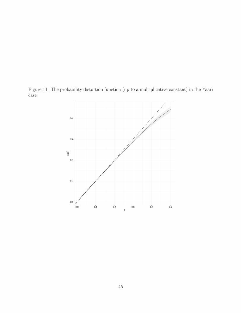
Figure 11: The probability distortion function (up to a multiplicative constant) in the Yaaricase

0.0

0.1

0.2

0.3

0.4

0.0 0.1 0.2 0.3 0.4 0.5p

G(p

)

45

Figure 12: The elasticity of the probability distortion function (up to a multiplicative con-stant in the RDEU case)

RDEU BIC Yaari BIC

0.5

0.6

0.7

0.8

0.9

1.0

0.0 0.1 0.2 0.3 0.4 0.5 0.0 0.1 0.2 0.3 0.4 0.5p

elas

ticity

of G

(p)

and in the above product, both terms (the elasticity of G with respect to p, and the fear of

ruin index associated to an expected utility maximizer) are only identified up to a common

positive constant. Figure 12 draws this elasticity as a function of the winning probability

on our preferred Yaari and RDEU homogeneous estimates. In the Yaari specification, this

elasticity is uniquely identified; in the RDEU specifications, we can only draw conclusions

on its variations. In both cases, the elasticity is rather flat at first, and then decreases for

probabilities above 0.3.

5.3.3 The general NEU model

Table 3 also shows that a general, homogeneous NEU model performs better than an ho-

mogeneous RDEU model. The former model also requires only one parameter, which makes

it especially parsimonious. This should be contrasted to the findings in Barseghyan, Moli-

nari, and O’Donoghue (2013) and many other works, who argue that probability distortions

are sufficient to explain the choices of deductible in car or auto insurance. These new esti-

46

Figure 13: Normalized fear-of-ruin for RDEU homogeneous

0.0 0.1 0.2 0.3 0.4 0.5

0.6

0.8

1.0

1.2

1.4

Probability

NF

●

●

●●●●●●●●

●●●●●●●

●●

●

● ●●●●●●●●●●●●●●●●

●

● ●●●●●●●●●●●●●●●●●●

●●●●●●●●●●●●●●●●●●●

●●●●●●●●●●●●●●●●●●●

●●●●●●●●●●●●●●●●●●●

●●●●●●●●●●●●●●●●●●●

R=1R=2R=4R=6R=10R=15R=20

mates may point to directions for which the RDEU model is too demanding. Unfortunately,

they are difficult to summarize, and we could not find a general feature that would make the

NEU model appear superior based on arguments other than statistical fit.24

A simple way to contrast the patterns predicted by the different NEU models is to plot

normalized fear of ruin NF(R, p) as a function of p for several fixed values of R. This is done

in Figures 13 and 14 for the RDEU and NEU homogeneous specifications. In both cases,

we plotted p → NF(R, p) for five values of R that range from large favorites to longshots.

The dashed vertical lines represent the corresponding risk-neutral probabilities, which give a

rough indication of where the simulated probabilities lie for given R. Notice the similarity of

the patterns: for each R, NF appears to be either a constant, either an increasing function of

p. Compared to the RDEU graph, NEU seems to allow for less departure from risk-neutrality,

thus giving the main role to probability distortions.

24Here is a curious illustration of this similarity. Recall from (16) that all models are the product ofp(R+ 1) and of the exponential of a polynomial K in (R, p). For the RDEU model, K is a linear polynomialin R, plus a quadratic polynomial in p (Table 8 in Appendix B); while for the NEU model, K is a polynomialin R, times a quadratic polynomial in p (Table 9). This shows both the power of our estimation strategyand the difficulty of understanding analytically the different effects.

47

Figure 14: Normalized fear-of-ruin for NEU homogeneous

0.0 0.1 0.2 0.3 0.4 0.5

0.6

0.8

1.0

1.2

1.4

Probability

NF

●

●

●●●

●●●●●●●●

●●●●●

●

● ● ●●●●●●●●●●●●●●●●●● ●●●●●●●●●●●●●●●●●●●●●●●●●●●●●●●●●●●●●

●●●●●●●●●●●●●●●●●●●

●●●●●●●●●●●●●●●●●●●

●●●●●●●●●●●●●●●●●●●

R=1R=2R=4R=6R=10R=15R=20

48

Figure 15: Isoquants of the normalized fear-of-ruin in the non-expected utility case

●

●

●

●

●

●

●

●

●

●

●

●

●

●

●

●

●

●

●

●

●

●

●

●

●

●

●

●

●

●

●

●

●

●

●

●

●

●

●

●

●

●

●

●

●

●

●

●

●

●

●

●

●

●

●

●

●

●

●

●

●

●

●

●

●

●

●

●

●

●

●●

●

●

●

●

●

●

●

●

●

●

●

●

●

●

●

●

●

●

●

●

●

●

●

●

●

●

●●

●

●

●

●

●

●

●

●

●

●

●

●

●

●

●

●

●

●

●

●

●

●

●

●

●

●

●

●●●

●

●

●

●

●

●

●

●

●

●

●

●

●

●

●

●

●

●

●

●

●●

●

●

●

●

●

●

●

●

●

●

●●

●

●

●

●

●

●

●

●

●

●

●

●

●

●

●

●

●

●

●

●

●

●

●

●

●

●●

●

●

●

●

●

●

●

●

●

●

●

●

●

●

●

●

●

●

●

●

●

●

●

●●

●

●●

●

●

●

●

●

●

●

●

●

●

●

●

●

●

●

●

●

●

●

●

●

●

●

●

●

●

●

●

●

●

●

●

●●

●

●

●

●

●●

●

●

●

●

●

●

●

●

●●

●

●

●

●

●

●

●

●

●

●

●

●

●

●

●

●

●

●

●

●

●

●

●

●

●

●

●

●

●

●

●

●

●

●

●

●

●

●

●

●

●

●

●

●

●

●

●

●

●

●

●

●

●

●

●●

●

●

●

●

●

●

●

●

●

●

●

●

●

●

●

●

●

●

●

●

●

●

●

●

●

●

●

●

●

●

●

●

●●

●

●

●

●

●

●

●

●

●●

●

●

●

●

●

●

●

●●

●●

●

●

●

●

●

●

●

●

●

●

●●

●

●

●

●●

●

●

●

●

●

●

●

●

●

●

●

●

●

●

●

●

●

●

●

●

●

●

●

●

●

●

●

●

●

●

●●

●

●

●

●

●

●

●

●

●

●●

●

●

●

●

●

●

●

●

● ●

●

●

●

●

●

●

●

●●

●

●

●

●

●

●

●

●

●

●

●

●

●

●

●

●

●

●

●●

●

●

●

●

●

●

●

●●

●

●

●

●

●

●

●

●

●

●

●

●

●

●

●

●

●

●

●

●

●

● ●

●

●

● ●

●

●

●

●

●

●

●

●

●

●

●

●

●

●

●

●

●

●

●

●

●

●

●

●

●

●

●

●

●

●

●

●

●

●●

●

●

●

●

●

●

●

●

●

●

●

●

●

●

●

●

●

●

●

●

●

●

●

●

●

●

●

●

●

●

●

●

●

●

●

●

●

●

●

●

●

●

●

●

●

●

●●

●

●

●

●

●●

●

●

●

●

●

●

●

●

●

●●

●

●

●

●

●

●

●

●

●

●

●

●

●

●

●

●

●

●

●

●

●

●

●

●

●

●

●

●

●

●

●

●

●

●

●

●

●

●

●

●

●

●

●

●

●

●

●

●

●

●

●

●

●

●

●

●

●

●

●

●

●

●

●

●●

●

●

●

●

●

●●

●

●

●●

●

●

●

●

●

●

●

●

●

●

●

●

●

●

●

●

●

●

●

●

●

●

●

●

●

●

●

●

●

●

●

●

●

●

●

●

●

●

●

●

●

●

●

●

●

●

●

●

●

●

●

●

●

●

●

●

●

●

●

●

●

●

●

●

●

●

●

●

●

●

●

●

●

●

●

●

●

●

●●

●

●●●

●

●

●

●

●

●

●●

●

●

●

●

●

●

●

●

●

●

●

●

●

●

●

●

●

●

●

●

●

●●

●

●

●

●

●

●

●

●

●

●

●

●

●

●

●

●

●

●

●

●●

●

●●

●

●

●

●●

●

●

●

●

●

●

●

●

●

●

●

●

●

●

●

●

●

●

●

●

●●

●

●

●●

●

●

●

●

●

●

●●

●

●

●

●

●

●

●

●

●

●

●

●

●

●

●

●

●

●

●

●

●

●

●

●

●

●

●

●

●

●

●

●

●

●

●

●

●

●

●

●

●

●

●

●

●

●

●

●●

●

●

●

●

●

●

●

●

●

●

●

●

●

●

●

●

●●

●

●

●

●

●

●

●

●

●

●

●

●

●

●

●

●

●

●

●

●

●

●

●

●

●

●

●

●

●

●

●

●

●

●

●

●

●

●

●

●

●

●

●

●

●

●

●

●

●

●

●

●

●

●

●

●

●

●

●

●

●

●

●

●

●

●

●

●

●

●

●

●

●

●

●

●

●

●

●

●

●

●

●

●

●

●

●

●●

●

●

●

●

●

●

●

●

●●

●

●

●

●

●

●

●

●

●

●

●

●

●●

●

●

●

●

●●

●

●●

●

●

●

●

●

●

●

●

●

●

●

●

●

●

●

●

●

●

●

●

●

●

●

●

●

●

●

●

●

●

●

●

●

●●

●

●

●

●

●

●

●

●

●

●

●

●

●

●

●

●

●

●

●

●

●

●

●

●●

●

●

●

●

●

●

●

●

●

●●

●

●

●

●●

●

●

●

●

●

●

●

●

●

●

●

●

●

●

●

●

●

●

●

●

●

●

●

●

●

●

●

●

●

●

●

●

●

●

●

●

●

●

●

●

●

●

●

●

●

●

●

●

●●

●

●

●

●

●

●

●

●

●

●

●

●●

●●

●●

●

●

●

●

●

●

●

●

●

●

●

●●

●

●

●

●

●

●

●

●

●

●

●

●

●

●

●

●

●

●

●

●

●

●

●

●

●

●

●

●

●

●

●

●

●

●

●

●

●

●

●

●

●

●

●

●

●

●

●

●

●

●

●

●

●

●

●

●

●●

●

●

●

●

●

●

●

●

●

●

●

●

●●

●

●

●●

●

●

●

●

●

●

●

●

●

●

●

●

●

●

●

●

●

●

●

●

●

●

●

●

●

●

●●

●

●

●

●

●

●

●

●

●

●

●

●

●

●

●

●

●

●

●

●

●

●

●

●

●

●

●

●

●

●●

●

●●●

●

●

●●

●

●

●

●

●

●

●

●

●

●

●

●

●

●

●

●

●

●

●

●

●

●

●

●

●

●

●

●

●

●

●

●

●

●●

●

●

●●

●

●

●

●

●

●

●

●

●

●

●

●

●

●

●

●

●

●

●

●

●

●

●

●

●

●

●

●

●

●

●

●

●

●

●

●

●

●

●

●●

●

●

●

●

●

●

●

●

●

●

●

●

●

●

●

●

●

●

●

●

●

●

● ●●

●

●

●

●

●

●

●

●

●

●

●

●

●

●

●

●●

●

●

●

●

●

●

●

●

●

●

●

●

●

●

●

●

●

●

●

●

●

●

●

●

●

●

●

●

●

●

●

●

●

●

●

●

●

●

●

●

●

●

●

●

●

●

●

●

●

●

●

●

●

●

●

●

●

●

●

●

●

●

●

●

●

●

●

●

●

●

●

●

●

●●

●

●

●

●

●

●

●●

●

●

●

●

●

●

●

●

●

●

●

●

●

●

●

●

●

●

●

●

●

●

●

●

●

●●

●

●

●

●

●

●

●

●

●

●

●

●

●●

●

●

●

●

●

●

●

●

●

●

●

●

●

●

●

●

●

●

●

●

●

●

●

●

●

●●

●

●

●

●

●

●

●

●

●

●

●

●

●●

●

●

●

●

●

●

●

●

●

●●

●

●

●

●●

●

●

●

●

●

●

● ●

●

●

●

●

●

●

●

●

●

●

●

●

●●

●

●

●

●

●

●

●

●

●

●

●

●

●

●

●

●

●

●

●

●

●

●

●

●

●

●

●

●

●

●

●

●●

●

●

●

●

●

●

●

●

●●

●

● ●

●

●

●

●

●

●

●

●

●

●●

●

●●

●

●

●

●

●

● ●

●

●●

●

●

●

●

●

●

●

●

●

●

●

●

●

●

●

●

●

●

●

●

●

●

●

●●

●

●●

●

●

●

●

●

●

●

●

●

●

●

●

●

●

●

●

●

●

●

●

●

●

●

●

●

●

●

●

●

●

●●

●

●

●

●

●

●

●●

●

●

●

●

●

●

●

●

●

●

●

●

●

●

●

●

●

●

●●

●

●

●

●

●

●

●

●

●

●

●

●

●

●

●

●

●

●●

●

●

●

●

●

●

●

●

●

●

●

●●

●

●

●

●

●

●●

●

●

●

●

●

●

●

●

●

●

●

●

●

●

●

●

●

●

●

●●

●

●

●

●

●

●

●

●

●

●

●

●

●

●

●

●

●

●

●

●

●

●

●

●

●

●

●

●

●

●

●

●

●

●

●

●

●

●

●

●

●

●

●

●

●

●

●

●

●

●

●

●

●

●

●

●

●

●

●

●

●

●

●

●

●●

●

●

●

●

●

●

●

●

●

●

●

●

●

●

●

●

●

●

●

●

●

●

●

●

●

●

●

●

●

●

●

● ●

●

●

●

●

●●

●

●

●

●

●●

●

●

●

●

●

●

●

●

●

●

●

●

●

●

●

●

●

● ●

●

●

●

●

●

●

●

●

●

●

●

●

●

●

●

●

●●

●

●●

●

●

●

●

●

●

●

●

●

●

●

●

●

●

●

●●

●

● ●

●

●

●

●

●

●

●

●

●

●

●

●

●

●

●

●

●

●

●

●

●

●

●

●

●

●

●

●

●

●

●

●

●

●

●

●

●

●

●

●

●●

●

●

●

●

●

●

●

●

●

●

●

●

●

●

●

●●

●

●

●

●

●

●

●

●

●

●

●

●

●

●

●

●

●

●

●

●

●

●

●

●●

●

●

●●

●

●

●

●

●

●

●

●

●

●

●

●

●

●

●

●

●

●

●

●

●

●

●

●

●

●

●

●

●

●

●

●

●

●

●

●

●

●

●

●

●

●

●

●

●

●

●

●

●

●

●

●

●

●

●

●

●

●

●

●

●

●

●

●

●

●

●

●●

●

●

●

●

●●

●

●

●●

●

●

●

●

●

●

●

●

●●

●

●

●

●

●

●

●

●

●

●

●

●

●

●

●

●

●

●

●

●

●

●

●

●

●

●

●

●

●

●

●

●

●

●

●

●

●

●

●

●

●

●

●

●

●

●

●

●

●●

●

●

●

●

●

●

●

●

●

●

●

●

●

●

●

●

●

●

●

●

●

●

●

●

●

●

●

●

●

●

●

●

●

●

●

●

●

●

●

●

●

●

●

●

●

●

●

●

●

●

●

●●

●

●

●

●

●●

●

●

●

●

●

●

●

●

●

●

●

●

●

●

●

●

●

●

●

●

●●

●

●

●

●

●

●●

●

●

●

●

●

●

●

●

●

●

●

●

●

●

●

●

●

●

●

●

●

●

●

●

●

●

●

●

●

●

●

●

●

●

●●

●

●

●

●

●

●

●

●

●

●

●

●

●

●

●

●

●

●

●

●

●

●

●

●

●

●

●

●

●

●

●

●

●

●

●

●

●

●

●● ●

●

●

●

●

●●

●

●

●

●

●

●

●

●

●

●

●

●●

●

●

●

●

●

●

●

●

●

●

●

●

●

●●

●

●

●

●●

●

●

●

●

●

●

●

●●

●

●

●●

●

●

●

●

●

●

●

●●

●

●

●

●

●

●

●

●

●

●

●

●

●

●

●

●●

●

●

●

●

●

●

●●

●

●

●

●

●

●

●

●

●

●

●

●

●

●

●

●

●

●

●

●

●

●

●

●

●

●

●

●

●

●

●

●

●

●

●

●

●

●

●

●

●

●

●

●

●

●

●

●

●

●●

●

●

●

●

●

●

●

●

●

●

●

●

●

●

●

●

●

●

●

●

●

●

●

●

●

●

●

●

●

●

● ●

●

●

●

●

●

●

●

●

●

●

●

●

●

●

●

●

●

●

●

●

●

●●

●

●

●

●●●

●

●

●

●

●

●

●

●

●

●

●

●

●

●

●

●

●

●

●

●

●

●

●

●

●

●●

●

●

●

●

●

●

●

●

●

●

●

●

●

●

●

●

●

●

●

●

●

●

●

●

●●

●

●

●

●

●

●

●

●●

●●

●

●

●

●

●

●●

●

●

●

●

●

●

●

●

●

●

●

●

●

●

●

●

●

●

●

●

● ●●

●

●

●

●

●

●

●

●

●

●

●

●

●

●

●

●

●

●

●

●

●

●

●

●

●

●●

●

●

●

●

●

●

●

●

●

●

●●

●

●

●

●

●

●

●

●

●

●

●

●

●

●

●

●

●

●

●

●

●

●

●

●

●

●

●

●

●

●

●

●

●●

●

●

●

●

●

●

●

●

●●

●

●

●

●

●

●

●

●

●

●

●

●

●

●

●

●

●

●

●

●

●

●●

●

●

●

●

●

●

●

●●

●

●

●

●●

●

●

●●

●

●

●

●

●

●

●

●

●

●

●

●

●

●

●

●

●

●

●

●●

●

●

●

●

●

●

●

●

●

●

●

●

●

●

●

●

●

●

●

●

●

●

●●

●

●

●

●

●

●●

●

●

●

●

●

●

●

●

●

●

●

●

●

●

●

●●●

●

●

●

●

●

●

●

●

●

●

●

●

●

●

●●

●

●

●

●

●

●

●

●

●

●

●

●

●

●

●

●

●

●

●

●

●

●

●

●

●

●

●

●

●

●

●

●

●

●

●

●●

●

●

●

●

●

●

●

●

●

●

●

●

●

●

●

●

●

●

●

●

●

●

●

●

●

●

●

●

●

●

●

●

●

●

●

●

●

●

●

●

●

●

●

●

●

●

●

●

●

●

●

●

●

●

●

●

●

●

●

●

●

●

●

●

●

●

●

●

●

●

●

●

●●

●

●

●

●

●

●

●

●

●

●

●

●

●

●

●

●

●

●

●

●

●

●

●

●

●

●

●

●

●

●

●

●

●

●

●

●

●

●

●

●

●

●

●

●

●

●

●

●

●

● ●●

●●

●

●

●

●

●

●

●

●

●

●

●

●

●

●

●

●

●

●

●

●

●

●

●

●

●

●

●

●

●

●

●

●

●

●

●

●

●

●

●●

●

●

●

●

●

●

●

●

●

●

●

●

●

●

●

●

●

●

●

●

●

●

●

●

●

●

●

●

●

●

●

●

●

●

●

●

●

●

●

●

●●

●

●

●

●

●

●

●

● ●

●

●

●

●

●

●

●

●

●

●

●

●

●

●●

●

●

●

●

●

●

●

●

●

●

●

●

●

●

●●

●

●

●

●

●

●

●

●

●

●

●

●

●

●

●

●

●

●

●

●

●

●

●

●

●

●

●

●

●

●

●

●

●

●

●

●

●

●

●

●

●

●

●

●

●

●

●

●●

●

●

●

●

●

●

●

●

●

●

●

●●

●

●

●

●

●

●

●

●

●

●●

●

● ●

●●

●

●

●

●

●

●

●

●

●

●

●

●

●

●

●

●

●

●

●

●

●

●

●

●

●

●

●

●

●

●

●●

●

●

●

●

●

●

●

●

●

●

●

●

●

●●

●

●

●

●

●

●

●

●

●

●

●

●

●

●

●

●

●

●

●

●

●

●

●

●

●

●

●

●

●

●

●

●

●

●●

●

●

●

●●

●

●

●

●

●

●

●

●

●

●

●

●

●

●

●

●

●

●

●

●

●

●

●

●

●

●

●

●

●

●

●

●

●

●●

●

●

●

●

●

●

●

●

●

●

●

●

●

●●

●

●

●

●

●

●

●

●

●

●

●

●

●

●

●

●

●

●

●

●

●

●

●

●

●

●

●

●

●

●

●

●

●

●●

●

●

●

●

●

●

●

●

●

●

●

●

●●

●

●

●●●

●

●

●

●

●

●

●

●

●

●

●

●

●

●

●

●

●

●

●

●

●

●

●

●

●

●

●

●

●

●

●

●

●

●

●

●

●

●

●

●

●

●

●

●

●

●

●

●

●

●

●

●

●

●

●

●

●

●

●

●

●

●

●

●●

●●

●

●

●

●

●

●

●

● ●

●

●

●

●

●

●

●

●

●

●

●

●

●

●

●

●

●

●

●

●

●

●

●

●●

●

●

●●

●

●

●

●

●

●

●

●

●

●

●

●●

●

●

●

●

●

●

●

●

●

●

●

●

●

●

●

●

●

●

●

●

●

●

●

●

●

●

●

●

●

●

●

●

●

●

●

●

●

●●

●

●

●

●

●

●

●

●

●

●

●

●

●●

●

●

●

●

●●

●

●

●

●

●

●

●

●

●

●

●●

●

●●

●

●●

●

●

●

●

●

●

●

●

●●

●

●

●

●

●

●

●●

●

●

●

●

●

●

●

● ●

●

●

●

●

●

●●

●

●

●

●

●

●

●

●

●

●

●

●

●

●

●

●

●

●

●

●

●

●

●

●

●

●

●

●

●

●

●

●

●

●

●

●

●

●

●

●

●

●

●

●

●

●

●

●

●

●

●

●

●

●

●

●

●

●

●

●

●

●

●

●

●

●

●

●

●

●

●

●

●

●

●

●

●

●

●

●

●

●

●

●

●

●

●

●

●

●

●

●

●

●

●

●

●

●

●

●

●●●

●

●

●

●

●

●

●

●

●

●

●

●

●

●

●●

●

●

●

●

●

●●

●

●

●

●

●●●

●

●

●

●

●

●

●

●

●

●

●

●

●

●

●●

●

●

●

●

●

●

●

●

●

●

●

●

●

●

●

●

●●

●

●

●

●

●●

● ●

●

●

●

●

●

●

●

●

●

●

●

●

●●

●

●

●

●

●

●

●

●

●

●

●

●

●●

●

●

●

●

●

●

●●

●

●

●

●

●

●

●

●

●

●

●

●

●

●

●

●

●

●

●

●

●

●

●

●

●●

●

●

●

●

●

●

● ●

●

●

●

●

●

●

●

●

●

●

●

●

●

●

●

●

●

●

●

●●

●

●

●

●

●

●

●

●

●

●

●

●

●

●

●

●

●

●

●

●

●

●

●

●

●

●

●

●

●

●

●

●

●

●

●

●

●

●●

●

●

●

●

●

●

●

●

●

●

●

●

●

●●

●

●

●

●

●

●

●

●

●

●

●

●

●

●

●

●

●

●

●

●●

●

●

●

●

●

●

●

●

●

●

●

●

●

●

●

●

●

●

●

●

●

●

●

●

●

●

●

●

●

●

●

●

●

●

●●

●

●

●

●

●

●

●●

●

●

●

●

●

●

●

●

●

●

●

●●

●

●

●

●

●

●

●

●

●

●

●

●

●

●

●

●

●

●

●

●

●

●

●

●

●

●

●

●

●

●●

●

●

●

●

●

●

●

●

●

●

●

●

●●

●

●

●

●

●

●

●

●

●

●

●

●

●

●

●

●

●

●

●

●

●

●

●

●

●

●

●

●

●

●

●

●

●

●

●

●

●

●

●

●

●

●

●

●

●

●

●

●

●

●

●

●

●

●

●

●

●

●

●

●

●

●

●

●

●

●

●

●

●

●

●●

●

●

●

●

●

●

●

●

●

●

●

●

●

●

●

●

●

●

●

●

●

●

●

●

●

●

●

●

● ●

●

●●

●

●

●

●

●

●

●

●

●●

●

●

●

●

●

●

●

●

●

●

●

●

●

●

●

●

●

●

●

●

●

●

●

●

●

●

●

●

●

●

●

●

●

●●●●

●

●

●

●

●

●

●

●

●

●

●

●

●

●●

●

●

●

●

●

●

●

●

●

●

●

●

●

●

●

●

●

●

●

●

●

●

●

●

●

●

●

●

●

●

●

●

●

●

●

●

●

●●

●

●

●

●

●

●

●

●

●

●

●

●●

●

●

●

●●

●

●

●

●●

●

●

●

●

●

●

●

●

●

●

●

●

●

●

●

●

●

●

●

●

●

●

●

●

●

●

●

●

●

●●

●

●

●

●

●

●

●

●

●

●

●

●

●

●

●

●

●

●

●

●

●

●

●

●

●

●

●

●

●

●

●

●

●

●

●

●

●

●

●

●

●

●

●

●

●

●

●

●

●

●

●

●

●

●

●

●

●

●

●

●

●

●

●

●

●

●

●

●●●

●●

●

●

●

●

●

●

●●

●

●

●

●

●

●

●

●

●

●

●

●

●

●

●

●●

●

●

●

●

●

●

●

●

●

●

●

●

●

●

●

●

●

●

●

●

●

●

●●

●

●

●

●

●

●

●

●

●

●

●

●

●

●

●●

●

●

●

●●

●

●●

●

●

●

●

●

●

●

●

●

●

●

●

●

●

●

●

●

●●

●

●

●

●

●

●

●

●

●●

●

●

●

●

●●

●

●

●

●

●

●

●

●●

●

●

●●

●

●

●

●

●

●●

●

●

●

●

●●

●

●

●●

●

●●

●

●

●

●

●

●

●

●

●

●

●

●●

●

●

●

●

●

●

●

●

●

●

●

●

●

●

●

●

●

●

●

●

●

●

●

●

●

●

●

●

●

●

●

●

●

●

●

●

●

●

●

●

●

●

●

●

●

●

●

●

●

●

●

●

●

●●

●

●

●

●

●

●

●

●

●

●

●

●

●

●

●

●

●

●

●

●

●●

●

●

●

●

●

●

●●

●

●

●

●

●

●

●●

●

●

●

●

●

●

●●

●

●

●

●

●

●

●

●

●●

●

●

●●

●

●

●

●

●

●

●

●

●

●

●

●

●

●

●

●

●

●

●

●

●●

●

●●

●

●

●

●

●

●

●

●●

●

●●

●

●

●●

●

●●

●

●

●

●

●

●

●

●

●

●

●

●

●

●

●

●

●

●

●

●

●

●

●●

●

●

●

●

●

●

●

●●

●

●

●

●

●

●

●

●

●

●

●

●

●●

●

●

●

●

●

●

●

●

●●

●

●

●

●

●

●

●

●

●

●●

●

●

●

●

●

●

●

●

●

●

●

●

●

● ● ●

●

●

●

●

●

●

●

●

●

●

●

●

●

●

●

●

●

●

●

●

●

●

●●

●

●●

●

●

●

●

●

●

●

● ●

●

●

●

●

●

●

●

●

●

●●

●

●

●

●

●

●

●

●

●

●

●

●

●

●

●

●

●

●

●●

●

●

●

●

●

●

●

●

●

●

●

●

●

●

●

●

●

●

●

●

●

●

●

●

●

●

●

●

●●

●

●

●

●

●

●

●

●

●

●

●

● ●

●

●

●

●

●

●

●

●

●

●

●

●

●

●

●

●

●

●

●

●●

●

●

●

●

●

●

●

●

●

●

●

●

●●

●

●

●

●

●

●●

●

●

●

●

●

●

●

●

●

●

●

●●

●

●

●

●

●

●

●●

●

●

●

●

●

●

●

●

●

●●

●

●

●

●

●●

●

●

●

●

●

●

●

●

●

●

●

●

●

●

●

●

●

●

●

●

●

●

●

●

●

●

●

●

●

●

●

●

●

●

●

●

●

●

●

●

●

●

●

●●

●

●

●

●

●

●

●

●

●

●

●

●

●

●

●

●

●

●

●

●

●

●

●

●

●

●

●

●

●

●

●●

●

●

●●

●

●

●

●

●

●

●

●

●●

●

●

●●

●●

●

●

●

●

●

●

●●

●

●

●

●

●

●

●

●

●

●

●

●

●

●

●

●

●

●

●

●

●

●

●

●

●

●

●

●

●

●●

●

●

●●

●

●●

●

●

●

●

●

●

●

●

●

●

●

●

●

●

●

●

●

●

●

●

●●

●

●

●

●

●

●

●

●

●

●

●

●

●

●

●

●

●

●

●

●

●

●

●

●

●

●

●●

●

●

●

●

●

●●

●

●

●

●

●

●

●

●

●

●●

●

●

●

●

●

●

●

●

●

●

●

●

●

●

●

●

●

●

●

●●

●

●

●

●

●

●

●

●

●

●

●

●

●

●

●

●

●

●

●

●

●

●

●

●●

●

●

●

●

●

●

●

●

●

●

●

●

●

●

●

●

●

●

●

●

●

●●

●

●

●

●

●

●

●

●

●

●

●

●

●

●

●

●

●

●

●

●

●

●

●

●

●

●

●

●

●

●

●

●

●

●

●

●

●

●

●

●●

●

●

●

●

●

●

●

●

●

●

●

●

●

●

●

●

●

●

●

●

●

●

●

●

●

●

●

●

●

●

●

●

●

●

●

●

●

●

●

●

●

●

●●

●

●

●

●●

●

●

●

●●

●

●

●

●

●

●

●

●

●

●

●

●

●

●

●

●

●

●

●

●

●

●

●

●

●●

●

●●

●

●

●

●

●●

●

●

●

●

●

●

●

●

●

●

●

●

●

●

●

●

●●

●

●

●

●●

●

●

●

●

●

●

●

●

●

●

●

●

●

●

●●

●

● ●●

●

●

●

●

●

●

●

●

●

●

●

●

●

●

●

●

●

●

●

●

●

●

●

●

●

●

●

●

●

●

●

●

●

●

●

●

●

●

●

●

●

●

●

●

●

●

●

●

●●

●

●

●

●

●●

●

●

●

●

●

●

●

●

●

●

●

●

●

●

●

●

●

●●

●

●

●●

●

●

●

●

●

●●

●

●

●

●

●

●

●

●

●

●

●

●

●

●

●

●

●

●

●

●

●

●

●

●

●

●

●

●

●

●

●●

●

●

●

●

●

●

●

●

●

●

●

●

●

●

●

●

●

●

●

●

●

●

●

●

●

●

●

●

●

●

●

●

●

●

●

●

●

●

●

●

●

●

●

●

●●

●

●●

●

●

●

●

●

●

●

●

●

●

●

●

●

●

●

●

●

●

●

●

●

●

●

●

●

●

●

●

●

●

●●

●

●

●

●

●

●

●

●

●

●

●

●

●●

●

●

●

●

●

●

●

●

●

●

●

●

●

●

●

●

●

●

●

●

●

●

●

●

●

●●

●

●

●

●

●

●●

●

●●●

●

●

●

●

●

●

●

●

●

●

●

●

●

●

●

●

●

●

●

●

●

●●

●

●

●

●

●

●

●

●

●

●

●

●

●

●

●

●

●

●

●

●

●●●

●

●

●

●

●

●

●

●

●

●

●

●

●

●

●

●

●

●

●

●

●

●

●

●

●

●

●

●

●

●

●

●

●

●

●

●

●

●

●

●

●

●

●

●

●

●

●

●

●

●

●

●

●

●

●

●

●

●●

●

●

●

●

●

●

●

●

●

●●

●●

●

●

●

●

●

●

●

●●

●

●●

●

●

●

●

●

●

●

●

●

●

●

●

●

●

●

●

●

●

●

●

●

●

●

●

●

●

●

●

●

●

●

●

●

●

●

●

●●

●

●

●

●

●

●

●

●

●

●

●

●

●

●

●

●

●

●

●

●

●

●

●

●

●

●

●

●

●

●

●

●

●

●

●

●

●

●

●

●

●

●

●

●

●

●

●

●●

●

●

●

●

●

●

●

●

●

●

●

●

●

●

●

●

●

●

●

●

●

●

●

●

●

●

●

●

●

●

●●

●

●

●

●●●

●

●

●

●

●

●

●

●

● ●

●

●

●

●

●

●

● ●

●

●

●

●

●

●

●

●

●

●

●

●

●

●

●

●

●●

●

●●

●

●

●

●

●

●

●

●

●

●

●

●

●

●

●

●

●

●

●

●

●

●

●

●●

●●

●

●

●

●

●

●

●

●

●

●

●

●

●

●

●

●

●

●

●

●

●

●

●

●

●●

●

●

●

●

●

●

●

●

●

●

●

●

●

●

●

●

●

●

●

●

●

●

●

●

●

●

●

●

●

●

●

●

●●

●

●

●●

●

●

●

●

●

●

● ●

●

●

●

●

●

●

●

●

●

●

●

●

●

●

●

●

●

●

●

●

●

●

●

●

●

●

●

●

●

●●

●

●

●

●

●

●

●

●

●

●

●

●

●

●

●

●

●

●

●

●

●

●

● ●

●

●

●

●

●

●

● ●

●

●

●

●

●

●

●

●

●

●●

●

●

●

●

●

●

●

●

●

●●

●

●

●

●

●

●

●

●

●

●

●

●

●

●

●

●

●

●

●

●

●

●

●

●

●

●

●

●

●

●

●

●

●

●

●

●

●

●

●●

●

●

●

●

●

●

●

●●

●●

●

●

●

●

●

●

●

●

●

●

●

●

●

●

●

●

●

●

●

●

●

●

●

●

●

●

●

●

●

●

●

●

●

●

●

●

●

●

●

●

●

●●

●

●

●

●

●

●

●

●

●

●

●

●

●

●

●

●

●

●

●

●

●

●

●

●

●

●

●

●

●

●

●

●

●

●

●

●

●

●

●

●

●

●

●

●

●

●

●

●●

●

●

●

●

●

●

●

●

●

●

●

●

●●

●

●

●

●

●

●

●

●

●

●

● ●

●

●

●

●

●

●

●

●

●

●

●

●

●

●

●

●

●

●

●

●

●

●

●

●

●

●

●

●

●

●

●

●

●

●

●

●

●

●

●

●●

●

●

●

●

●

●

●

●

●

●

●

●

●●

●

●

●

●

●●

●

●

●

●

●

●

●

●

●

●

●

●

●

●

●

●

●

●

●

●

●

●

●

●

●

●

●

●

●

●

●

●

●

●

●●

●

●

●

●

●

●

●

●

●

●

●

●

●

●

●

●

●

●

●

●

●

●

●

●

●

●

●

●

●

●

●

●

●

●

●

●

●

●●

●

●

●●

●

●

●

●

●

●

●

●

●

●

●

●

●●

●

●

●

●

●

●

●

●

●

●

●

●

●

●

●

●

●

●

●

●

●

●

●

●

●

●

●●

●

●

●

●

●

●

●

●

●

●

●

●

●

●●

●

●

●

●

●

●

●

●

●

●

●

●

●

●●

●

●

●

●

●

●

●

●●

●

●

●

●

●

●

●

●

●

●

●●

●

●

●

●

●

●

●

●

●

●

●

●

●

●

●

●

●

●

●

●

●

●

●

●

●

●

●

●●

●

●

●

●

●

●

●

●

●

●

●

●

●

●

●●

●

●

●

●

●

●

●

●

●

●

●

●

●

●

●

●

●

●

●

●

●

●

●

●●

●

●

●

●

●

●

●

●

●

●

●

●

●

●

●

●

●

●

●

●

●

●

●

●

●

●

●

●

●

●

●

●

●

●

●

●

●

●

●

●

●

●

●

●

●

●

●

●

●●

●

●●

●

●●

●

●

●

●

●

●

●

●

●

●

●

●

●

●

●

●

●

●

●

●

●

● ●

●

●

●

●

●

●

●

●

●

●

●

●

●

●

●

●

●

●

●

●

●

●●

●

●

●●

●

●

●

●●

●

●

●

●

●

●

●

●

●

●

●

●

●

●

●

●

●

●

●

●

●

●

●

●

●

●

●

●

●

●

●

●

●

●

●

●

●

●

●

●

●

●

●

●

●●

●

●

●●

●●

●

●

●

●

●

●

●

●

●

●

●

●

●

●

●●

●

●

●

●

●

●

●

●

●

●

●

●

●

●

●

●

●

●

●

●

●

●

●

●

●

●●

●

●

●

●

●

●

●

●●

●

●

●

●

●

●

●

●

●

●

●

●

●●

●

●

●

●

●

●

●

●

●

●

●

●

●

●

●

●●

●

●

●

●

●

●

●

●

●

●

●

●

●

●

●

●

●

●

●

●

●

●

●

●

●

●

●

●

●

●

●●

●

●

●

●

●

●

●

●

●

●

●

●

●

●

●

●

●

●

●

●

●

●

●

●●

●●

●●

●

●

●

●

●

●

●

●●

●

●●

●

●

●

●

●

●

●

●

●

●

●

●

●

●

●

●

●

●●

●

●

●

●

●

●

●

●

●

●

●

●

●●

●

●

●

●

●

●

●

●

●

●

●

●

●

●

●

●

●

●

●●

●

●

●

●

●

●

●

●

●

●

●

●●

●

●

●

●●

●

●

●

●

●

●

●

●

●

●

●

●

●

●

●

●●

●

●

●

●

●

●

●

●

●

●

●

●

●

●

●●

●

●

●●

●

●

●

●

●

●

●

●

●

●

●

●

●●

●●

●

●

●

●

●

●

●

●●

●

●

●

●

●

●

●

●

●

●

●

●

●

●

●

●

●

●

●

●

●

●

●

●

●

●

●

●

●

●

●

●

●

●

●●

●

●●

●

●

●

●

●

●

●

●

●

●

●

●

●

●

●

●●

●

●

●

●

●

●

●

●

●

●

●

●

●

●

●

●

●

●

●

●

●

●

●

●

●

●

●

●

●

●

●

●

●●

●

●

●

●

●

●

●

●

●

●

●

●

●

●●

●●

●

●

●

●

●

●

●

●

●

●

●

●●

●

●

●

●

●

●

●

●

●

●

●

●

●

●

●

●

●

●

●

●

●

●●

●

●

●

●

●

●

●

●

●

●

●

●

●

●

●

●

●

●

●

●

●

●

●

●

●

●

●

●

●

●

●

●●

●

●

●

●

●

●

●

●

●

●

●

●

●

●

●●

●

●

●

●

●

●

●

●

●

●

●

●

●

●

●

●

●

●

●

●

●

●

●

●

●

●

●

●●

●

●

●

●

●

●

●

●

●

●

●

●

●

●

●

●

●

●

●

●

●

●

●

●

●

●

●

●

●

●

●

●

●

●

●

●

●

●

●

●

●

●

●

●

●

●

●

●

●

●

●

●

●

●

●

●

●

●

●

● ●

●

●

●

●●

●

●

●

●● ●

●●

●●

●

●

●

●

●

●

●

●

●

●

●

●

●

●

●

●

●

●

●

●

●

●

●

●

●

●

●

●

●

●

●

●

●

●

●

●

●

●

●

●

●

●

●

●

●

●

●

●

●

●

●

●

●

●

●

●

●

●

●

●

●

●

●

●

●

●

●

●

●

●

●

●

●

●

●

●

●

●

●●

●

●

●

●

●

●

●

●

●

●

●

●

●

●

●

●

●

●

●

●

●

●

●

●

●

●

●

●

●

●

●

●

●

●

●

●

●

●

●

●

●

●

●

●

●

●

●

●

●

●

●

●

●

●

●

●●

●

●

●

●

●

●

●

●

●

●

●

●

●

●

●●

●

●

●

●

●

●

●

●

●

●

●

●

●

●

●●

●

●

●

●

●

●

●

●

●

●

●

●

●

●

●

●

●

●

●

●

●

●

●

●

●

●

●

●

●

●

●

●

●

●

●

●

●

●

●

●

●

●

●

●

●

●

●

●

●

●

●

●

●

●

●

●

●

● ●●

●

●

●

●●

●

● ●

●

●

●●

●

●

●

●

●

●

●

●

●

●

●

●

●

●

●

●●

●

●

●

●

●

●

●

●

●

●

●

●

●

●

●

●●

●

●

●

●

●

●●

●●

●

●

●

●

●

●

●

●

●

●

●

●

●

●

●

●

●● ●

●

●

●

●

●

●

●

●

●

●

●●

●

●●

●

●

●

●

●

●

●

● ●

●

●

●

●

●

●

●

●

●

●

●

●

●

●

●

●

●

●

●●

●

●

●●

●

●

●

●

●

● ●●

●

●

●

●

●

●

●

●

●

●

●

●

●

●

●

● ●

●

● ●

●

●

●

●

●

●

●

●

●

●

●

●

●●

●

●

●

●

●

●

●

●

●

●

●

●●

●

●

●

●

●

●

●

●

●

●

●

●

●

●

●●

●

●

●

●

●

●

●

●

●

●

●

●

●

●

●

●

●

●

●

●

●

●

●

●

●

●

●

●

●

●

●

●

●

●

●

●

●●

●

●

●

●●

●

●

●

●

●

●

●

●

●

●

●

●

●

●

●

●

●

●

●

●

●

●

●

●

●

●

●

●

●●

●

●

●

●

●

●

●

●

●

●

●

●

●

●

●

●

●

●

●

●

●

●

●

●

●

●

●

●

●

●

●

●

●

●

●

●

●

●

●

●

●

●

●

●

●

●

●

●

●

●

●

●

●

●

●

●

●

●

●

●

●

●

●

●

●

●

●

●

●

●

●

●●

●

●

●●

●

●

●●

●

●

●

●

●

●

●

●

●

●

●

●

●●

●

●

●

●

●

●

●

●

●

●

●

●

●

●

●

●

●

●

●

●

●

●

●

●

●

●

●

●

●

●

●

●

●

●

●

●

●

●

●

●

●

●

●

●

●

●

●

●

●

●

●

●

●

●

●

●

●

●

●

●

●

●

●

●

●

●

●●

●

●

●

●

●

●

●

●

●

●

●

●

●

●

●

●

●

●

●

●

●

●

●

●

●

●

●

●

●

●

●

●

●●

●

●

●

●

●

●

●

●

●

●

●

●

●

●

●

●

●

●

●●

●

●

●

●

●

●

●

●

●

●

●

●

●

●

●

●

●

●

●

●

●

●

●

●

●

●●

●

●

●

●

●

●

●

●

●

●

●

●

●

●

●

●

●

●

●

●

●

●

●

●

●

●

●

●

●

●

●

●

●

●

●

●

●●

●

●

●

●

●

●

●

●

●

●

●

●

●●

●

●

●

●

●

●

●

●

●

●

●

●●

●

●

●

●

●

●

●

●

●

●●

●

●

●

●●

●

●

●

●

●

●

●

●

●

●

●

●

●

●

●

●●

●

●

●

●

●

●

●

●

●

●

●

●

●

●

●

●

●

●

●

● ●

●

●

●

●

●

●

●

●

●

●

●

●

●

●

●

●

●

●

●

●

●

●

●

●

●

●

●

●

●

●

●

●

●

●

●

●

●

●

●

●

●●

●

●●

●

●

●

●

0.8 0.80.9 0.9 0.91 1 1●

●

●

●

●

●

●

●

●

●

●

●

●

●●

●

●

●

●

●

●

●

●

●

●

●

●

●

●

●

●

●

●

●

●

●

●

●

●

●

●

●

●

●

●

●

●

●

●

●

●

●

●

●

●

●

●

●

●

●

●

●

●

●

●

●

●

●

●

●

●

●

●

●

●

●

●

●

●

●

●

●

●

●●

●

●

●

●

● ●

●

●

●

●

●

●

●

●●

●

●

●

●

●

●

●

●

●

●

●

●

●

●

●

●

●

●

●

●

●

●

●

●

●

●

●

●

●

●

●

●

●

●

●

●

●

●

●●

●

●

●

●

●

●●

●

●

●

●

●

●●

●

●

●

●

●

●

●

●●

●

●

●

●

●

●

●

●

●

●

●

●

●

●

●

●

●●

●

●

●

●

●

●

●

●

●

●

●

●

●

●●

●

●

●

●

●

●

●

●

●

●

●

●

●

●●

●

●

●

●

●

●

●

●

●

●

●

●

●

●

●

●

●

●

●

●

●

●

●

●

●

●

●

●

●

●

●

●

●

●

●●

●

● ●

●

●

●

●

●

●

●

●

●

●

●

●

●

●

●

●

●

●

●

●

●

●

●

●

●

●

●

●

●

●

●

●

●

●●

●

●

●●

●

●

●

●

●●

●

●

●

●

●

●

●

●

●

●

●

●

●

●●

●

●

●

●

●

●

●

●

●

●

●

●

●

●

●

●

●

●

●

●

●

●

●

●

●

●

●

●

●

●

●

●

●

●

●

●

●●

●

●

●

●

●

●

●

●

●

●

●

●

●

●

●

●

●

●

●

●

●

●

●

●

●

●

●

●

●

●

●

●

●

●

●

●●

●

●

●

●

●

●

●

●

●

●

●●

●

●

●

●

●

●

●

●

●

●

●

●

●

●

●

●

●

●

●

●●

●

●

●

●

●

●

●

●

●

●

●

●

●

●

●

●

●

●

●

●

●

●

●

●

●

●

●

●

●

●

●●

●

●

●

●

●

●

●

●

●

●

●

●●

●

●

●

●

●

●

●

●

● ●

●●

●

●

●

●●●

●

●

●

●●

●

●

●

●●

●

●

●

●

●

●

●

●

●

●

●●

●

●

●

●

●

●

●

●

●

●

●●

●

●

●

●

●

●

●

●

●

●

●

●

●

●

●

●

●

●

●●

●

●

●

●

●

●

●

●

●

●

●

●

●

●

●

●

●

●

●

●

●

●

●

●

●

●

●

●

●

●

●

●

●

●

●

●

●

●

●

●●

●

●

●

●

●●

●

●

●

●

●

●

●

●

●

●

●

●

●

●

●

●

●

●

●

●

●

●

●

●

●

●

●

●

●

●

●

●

●

●

●

●

●

●

●

●

●

●

●

●

●

●

●

●

●

●

●

●

●

●

●

●

●●

●

●

●

●

●

●

●

●

●

●

●

●

●

●

●

●

●

●

●

●

●

●

●

●

●

●

●

●

●

●

●●

●

●

●

●

●●

●

●

●

●

●

●

●

●

●

●

●

●

●

●

●●

●

●●

●

●

●

●

●

●●

●

●

●

●

●

●

●

●

●

●

●

●

●

●

●

●

●

●

●

●

●●●

●

●

●●

●

●

●●

●●

●

●

●

●

●

●

●

● ●

●

●

●

●

●

●

●

●

●

●

●

●

●

●

●●

●

●

●

●

●

●

●

●

●

●

●

●

●

●

●

●

●

●

●

●

●

●

●

●

●

●

●

●

●

●

●●

●

●

●

●

●

●●

●

●

●

●

●

●

●

●

●

●

●

●●

●

●

●

●

●

●●

●●

●

●

●

●

●

●

●

●

●

●

●

●

●

●

●

●

●

●

●

●

●

●

●

●

●

●

●

●

●

●

●

●

●

●

●

●

●

●

●

●

●

●

●

●

●

●

●

●

●

●

●

●

●

●

●●

●

●

●

●

●

●

●

●

●

●

●

●

●

●

●

●

●

●

●

●

●

●

●

●

●

●

●

●

●

●

●

●

●

●

●

●

●

●

●

●

●

●

●

●

●

●

●

●

●

●

●

●

●

●

●

●

●

●

●

●

●

●

●●

●

●

●●

●

●

●

●

●

●

●

●

●

●

●

●

●

●

●

●●

●

●

●

●

●

●

●

●

●

●

●

●

●

●

●

●

●

●

●

●

●

●●

●

●

●

●●

●

●

●

●

●

●●

●

●

●

●

●

●

●

●

●

●

●

●

●

●

●

●●

●

●

●

●●

●

●

●

●

●

●●

●

●

●

●

●

●

●●

●

●

●

●

●

●

●

●

●

●●

●

●

●

●

●

●

●

●

●

●

●

●

●

●

●

●

●

●

●

●

●

●

●

●

●

●

●

●●

●

●

●

●

●●

●

●

●

●

●

●

●

●

●

●

●

●

●

●

●

●

●

●

●

●

●

●

●

●

●

●

●

●

●

●

●

●

●

●

●●

●

●

●

●

●

●

●

●

●

●

●

●

●

●

●

●

●

●

●

●

●●

●

●

●

●

●

●

●

●

●

●

●

●

●

●

●

●

●

●

●

●

●

●

●

●

●

●

●

● ●

●

●

●

●

●●

●

●

●

●

●

●

●

●

●

●

●

●

●

●

●

●

●

●

●

●

●

●

●

●

●

●

●

●

●

●

●

●

●

●

●

●

●

●

●

●●

●

●

●

●

●

●

●

●

●

●

●

●●

●

●

●

●

●

●

●

●

●

●

●●

●●

●

●

●

●

●

●

●

●

●

●

●

●

●

●

●

●

●

●

●

●

●●

●

●

●●

●

●

●

●

●

●

●

●

●

●

●

●

●

●

●

●

●

●

●

●

●

●

●

●

●

●

●

●●

●●

●

●

●

●

●

●

●

●

●

●

●●

●

●

●

●

●

●

●

●

●

●

●● ●

●

●

●

●●

●

●

●

●

●

●

●●

●

●

●

●

●

●

●

●

●

●

●

● ●

●

●

●

●

●

●

●

●

●

●

●

●

●

●

●

●

●

●

●

●

●

●

●

●

●

●

●

●

●●

●

●

●

●

●

●

●

●

●

●

●

●

●

●

●

●

●

●

●

●

●

●

●

●

●

●

●

●

●

●

●

●

●

●

●

●

●

●

●

●

●

●

●

●

●

●

●

●

●

●

●

●

●

●

●

●

●

●

●

●

●

●

●

●

●

●

●

●

●

●

●

●

● ●

●

●

●

●

●

●

●

●

●

●

●

●

●

●

●

●

●

●

●

●

●

●

●

●

●

●

●

●●

●

●●

●

●

●

●

●● ●

●

●

●

●

●

●

●

●

●

●

●

●

●

●

●

●

●

●

●

●●

●

●

●

●

●

●

●

●

●

●

●

●

●

●

●

●

●

●

●

●

●

●

●

●

●

●●

●

●

●

●

●

●

●

●

●

●

●

●

●

●

●

●

●●

●

●●

●

●

●

●

●

●

●

●

●

●

● ●

●

●

●

●

●

●

●●

●

●

●

●

●

●

●

●

●

●

●

●

●

●

●

●

●

●

●

●

●

●

●

●●

●

●

●

●

●

●

●

●

●

●

●

●

●

●

●

●

●

●

●

●

●

●

●●●

●

●

●

●

●

●

●

●

●

●

●

●

●

●

●

●

●

●

●

●

●

●

●

●

●

●

●

●

●

●

●

●

●

●

●

●

●

●

●

●

●

●

●

●

●

●

●

●

●

●

●

●

●

●●

●

●

●

●

●

●

●●

●

●

●

●

●

●

●

●

●

●

●●

●●

●●

●

●

●

●

●

●

●

●

●

●

●

●

●

●

●

●

●

●

●

●

●●

●

●●

●

●

●

●

●

●

●

●

●

●

●

●

● ● ●●

●

●

●

●

●

●

●

●

●

●

●

●

●

●

●

●

●

●

●

●

●

●

●

●

●

●

●

●

●

●

●

●

●

●

●

●

●

●

●

●

●

●●

●

●

●

●

●

●

●●

●

●

●

●

●

●

●

●

●

●

●

●

●

●

●

●

●

●

●

●

●●

●

●

●

●

●

●

●

●

●

●

●

●

●

●

●

●

●

●

●

●

●

●

●

●

●

●

●

●

●

●

●

●

●

●

●

●

●

●

●

●

●

●

●

●

●

●

●

●

●●

●

●

●

●

●

●

●

●

●

●

●

●

●

●

●

●

●●

●●

●

●●

●

●

●

●

●

●

●

●

●

●

●

●

●

●

●

●

●

●

●

●

●

●

●

●

●

●

●

●

●

●

●

●

●

●

●

●

●

●

●

●

●

●

●

●

●

●

●

●

●

●

●

●

●

●

●

●

●

●

●

●

●

●

●

●

●●

●

●

●

●

●

●

●

●

●

●

●

●

●

●

●

●

●

●

●●

●

●

●

●

●

●

●

●

●

●

●

●

●

●

●

●

●

●

●

●

●

●

●

●

●

●

●

●

●

●

●

●

●

●

●

●

●

●

●

●

●●

●

●

●

●

●

●

●

●

●

●

●

●

●

●

●

●

●

●

●

●

●

●

●

●

●

●

●

●

●

●

●

●

●

●

●

●

●

●

●

●

●

●

●

●

●

●

●

●

●

●

●

●

●

●●

●

●

●

●

●

●●

●

●●

● ●

●

●●

●

●

●

●

●

●

●

●

●

●

●

●

●

●●

●

●

●

●

●

●●

●

●

●

●

●

●

●

●

●

●

●

●

●

●

●

●

●

●

●

●

●

●

●

●

●

●

●

●

●

●●

●

●

●

●

●

●

●

●

●

●

●

●

●

●

●

●

●

●

●

●

●

●

●

●

●

●

●

●

●

●

●

●

●

●

●

●

●

●

●

●

●

●

●

●

●

●

●

● ●

●●

●

●

●

●

●

●

●

●

●

●

●

●

●

●

●

●

●

●

●

●

●

●

●

●

●

●

●

●

●

●

●

●

●

●

●

●

●●

●

●●

●

●

●

●

●

●

●

●

●

●

●

●

●

●

●

●

●

●

●

●

●

●

●

●

●

●

●

●

●

●

●

●

●

●

●

●

●

●●

●

●

●

●

●●

●

●

●

●

●

●

●

●

●●

●

●

●

●

●

●

●

●

●

●

●

●

●

●

●

●

●

●

●

●

● ●

●

●

●

●

●

●●

●

●

●

●

●

●

●

●

●

●

●

●

●

●

●

●

●

●

●

●

●

●

●

●

●●

●

●

●

●

●

●

●

●

●

●

●

●

●

●

●

●

●

●

●

●

●

●●

●

●

●

●

●

●

●

●

●

●

●

●●

●

●●

●

●

●

●

●

●

●

●

●

●●

●

●

●

●

●

●

●

●

●

●

●

●

●

●

●

●

●

●

●

●

●

●

●

● ●

●

●

●

●

●

●

●●

●

●

●

●

●

●

●

●

●

●

●

●

●

●

●

●

●

●

●

●

●

●

●

●

●

●

●

●

●●

●

●

●●

●

●

●

●

●

●

●

●

●

●

●

● ●

●

●

●

●

●

●

●

●

● ●

●

●

●

●●

●

●

●●

●

●

●

●

●●

●

●

●

●

●

●

●

●

●

●

●

●

●

●

●

●

●

●

●●

●

●● ●

●

●

●

●

●

●

●

●

●

●

●●

●●

●

●

●

●

●

●

●

●

●

●

●

●

●

●

●

●

●

●

●

●

●

●

●

●

●

●

●

●

●

●

●●

●

●

●

●

●

●

●

●

●

●

●

●

●

●

●

●

●

●

●

●

●

●

●

●

●

●

●

●

●

●

●

●●

●

●

●

●

●

●●●

●

●

●

●

●

●

●

●

●

●

●

●

●

●

●

●

●

●

●

●

●

●

●

●

●

●

●

●

●

●

●

●

●

●

●

●

●

●

●

●

●

●

●

●

●

●

●

●

●

●

●

●

●

●

●

●

●

●

●

●

●

●

●

●

●

●

●●

●

●

●

● ●

●

●

●

●

●

●

●

●

●

●

●

●

●

●

●●

●

●

●

●

●

●

●

●

●

●

●

●

●

●

●

●

●

●

●

●

●

●

●

●

●

●

●

●

●

●

●

●

●

●

●

●

●

●

●

●

●

●

●

●

●

●

●

●

●

●

●

●

●

●

●

●

●

●

●

●

●

●

●

●

●

●

●

●

●

●

●

●

●

●

●

●

●

●

●

●

●

●●

●

●

●

●

●

●●

●●

●

●

●

●

●

●

●●

●

●

●

●

●

●

●●

●

●

●

●

●

●

●

●

●

●●

●

●

●●

●

●

●

●

●

●

● ●

●

●

●

●

●

●

●

●

●

●

●

●

●

●

●

●

●

● ●

●

●

●

●

●

●●

●

●

●

●

●

●

●

●

●

●

●●

●

●

●

●

●

●

●

●

●

●

●

●

●

●

●

●●

●

●

●

●

●

●

●

●

●

●

●

●

●

●

●

●

●

●

●

●

●

●

●

●

●

●

●

●

●

●

●

●

●

●

●●

●

●

●

●

●

●

●

●

●

●

●

●

●

●

●

●

●

●

●

●

●

●

●

●

●

●

●

●

●

●

●

●

●

●

●

●

●

●

●

●

●

●

●

●

●

●

●

●

●

●

●

●

●

●●

●

●

●

●

●

●

●

●

●

●

●

●

●

●

●

●

●

●

●

●

●

●

●

●●

●

●

●

●

●●

●

●

●

●

●

●

●●

●

●

●

●

●

● ●

●

●

●

●

●

●

●

●

●

●

●

●

●

●

●

●

●

●

●

●

●

●

●

●

●

●

●

●

●●

●

●

●

●

●

●

●

●

●

●

●

●

●

●

●

●

●

●

●

●●

●

●

●

●

●

●

●

●

●

● ●

●

●

●

●

●

●

●

●

●

●

●

●

●

●

●

●●

●

●

●

●

●

●

●

●

●

●

●

●

●

●

● ●

●

●

●

●●

●

●

●

●

●

●

●●

●

●

●

●

●

●

●

●

●

●

●

●

●

●

●

●

●

●

●

●

●

●

●

●

●

●

●

●

●●

●

●

●

●

●

●

●

●

●

●

●

●

●

●

●

●

●

●

●

●

●

●

●

●

●

●

●

●

●

●

●

●

●

●

●

●

●

●

●

●

●

●

●

●

●

●

●●

●

●

●

●

●

●

●

●

●

●

●

●

●

●

●

●

●

●

●

●

●

●

●

●

●

●

●

●

●

●

●

●

●

●

●

●

●

●

●

●

●

●

●

●

●

●

●

●

●

●

●

●

●

●

●

●

●

●

●

●

●

●

●

●

●

●

●

●

●

●

●

●

●

●

●

●

●

●

●

●

●

●

●

●

●

●

●

●

●

●

●

●

●

●

●

●

●

●

●●

●

●

●

●

●

●

●

●

●

●

●

●

●

●●

●

●

●

●

●

●

●●

●

●

●●

●

●

●

●

●

●●

●●

●

●

●

●

●

●

●

●

●

●

●

●

●

●

●

●

●

●

●

●

●●

●

●

●

●

●

●●

●

●

●

●

●

●

●●●

●

●

●●

●

●

●

●

●●

●

●

●

●

●

●

●

●

●

●

●

●

●

●

●

●

●

●

●

●

●

●

●

●

●

●

●

●

●

●

●

●

●

●

●

●

●

●

● ●

●

●

●

●

●

●

●

●

●

●

●●

●

●

●

●

●

●

●

●

●

●

●

●

●

●

●

●

●

●

●

●

●

●

●

●

●

●

●

●

●

●

●

●

●

●

●

●

●

●

●

●

●

●

●

●

●

●

●

●

●

●

●

●

●

●

●

●

●

●

●

●

●

●

●

●

●

●

●

●

●

●

●

●

●

●

●

●●

●

●

●

●

●

●

●●

●

●

●

●

●

●

●

●

●

●

●

●

●

●

●

●

●

●

●

●

●

●

●

●

●

●

●

●

●

●

●

●

●●

●

●

●

●

●●

●

●

●●

●

●

●

●

●

●

●

●

●

●

●

●●

●

●

●

●

●

●

●

●

●

●

●

●

●

●

●

●

●

●

●

●

●

●

●

●

●

●

●

●

●

●

●

●

●

●

●

●

●

●

●

●

●

●

●

●

●

●

●

●

●

●

●

●

●

●

●

●

●

●

●

●

●

●

●

●

●

●

●

●

●

●

●

●

●

●

●●

●

●

●

●

●

●

●

●

●

●

●

●

●

●●

●

●

●

●

●

●

●

●

●

●

●

●

●

●

●

●

●

●●

●

●

●

●

●

●

●

●

●

●

●

●

●

●

●

●

●

●

●

●

●

● ●

●

●

●

●

●

●

●

●

●

●

●●

●

●

●

●

●

●

●

●

●

●

●

●

●

●

●

●

●

●

●

●

●

●

●

●

● ●

●

●

●

●

●

●

●

●

●

●

●

●

●

●

●

●●●

●

●

●

●

●

●

●

●●

●

●

●

●●

●

●

●

●

●

●

●

●

●●

●

●

●

●

●

●

●

●

●

●●

●

●

●

●

●

●

●

●

●

●●

●

●

●

●

●

●

●

●

●

●

●

●

●

●

●

●

●

●

●

●

●

●

●

●

●

●

●

●

●

●

●●

●

●

●

●

●

●

●

●●

●

●

●

●

●

●

●

●

●

●

●

●

●

●

●

●

● ●

●

●●

●

●

●

●●

●

●

● ●

●

●

●

●

●

●

●

●

●

●

●●

●

●

●

●

●

●

●

●

●

●

●

●

●

●

●

●

●●

●

●

●

●

●

●

●

●●

●

●●

●

●

●

●

●

●

●

●

●

●

●

●

●

●

●

●

●

●

●

●

●

●

●

●

●

●

●

●

●

●

●

●

●

●

●

●

●●

●

●

●

●

●●

●

●

●

●

●

●

●

●

●

●

●

●

●

●

●

●●

●

●

●

●

●●

●

●

●

●

●

●

●

●●

●

●

●

●

●

●

●

●

●

●

●

●

●

●

●

●

●

●

●

●

●

●

●

●

●

●

●

●

●

●

●

●

●

●

●

●

●

●

●

●

●

●

●

●

●

●

●

●

●

●

●

●

●

●

●

●

●

●

●

●

●

●

●

●

●

●

●

●

●

●

●

●

●

●

●

●

●

●

●

●

●

●

●

●

●

●

●

●

●

●

●

●

●

●

●

●

●

●

●

●

●

●

●

●

●

●

●

●●

●

●

●

●

●

●

●

●

●

●

●

●●

●

●

●

●

●

●

●

●●

●

●

●

●

●●

●

●

●

●

●

●

●

●

●

●●

●

●

●

●

●

●

●

●

●

●

●

●

●

●

●

●

●

●

●

●

●

●

●

●

●

●

●

●

●

●

●●

●

●

●

●

●

●

●

●

●

●

●

●

●

●

●

●

●

●

●●

●

●

●●

●

●●

●

●

●

●

●●

●

●

●

●

●

●

● ● ●●

●

●

●

●

●

●

●

●

●

●

●

●

●●

●

●

●

●

●

●

●

●

●

●

●

●

●

●

●

●

●

●

●

●

●

●

●

●

●

●

●

●

●

●

●

●

●

●

●

●

●●

●●

●

●

●●

●

●

●

●

●

●

●

●

●

●

●

●

●

●

●

●

●

●

●

●

●

●

●

●

●

●

●

●

●

●

●

●

●

●●●

●

●

●

●

●

●

●

●

●●

●

●●

●

●

●

●

●

●

●

●

●

●

●

●

●

●

●

●

●

●

●

●

●

●

●

●

●

●

●

●●

●

●

●

●

●●

●

●

●

●

●●

●

●

●

●●

●

●

●

●

●

●

●

●

●

●

●

●

●

●●

●

●

●

●

●

●

●

●

●

●

●

●●

●

●

●

●

●

●

●

●

●

●

●

●

●

●●

●

●

●

●

●

●

●

●

●

●

●

●

● ●

●

●

●

●

●

●

●

●

●●

●

●

●

●

●

●

●

●

●

●

● ● ●●

●

●

●

●

●

●●

●

●

●●

●

●

●

●

●

●

●

●

●

●

●

●

●

●

●

●

●

●

●

●

●

●

●

●

●

●

●

●

●

●

●

●

● ●

●

●

●

●

●

●●

●

●

●

●

●

●

●

●

●

●

●

●

●

●

●

●

●

●

●

●

●

● ●

●

●

●

●

●

●

●

●

●

●

●

●

●

●

●

●

●

●

●

●

●

●

●

●

●

● ●●

●

●

●

●

●

●

●

●●

●

●

●

●

●

●

●

●

●

●

●●

●

●

●

●

●

●

●

●

●

●

●

●

●

●

●

●

●

●

●

●

●

●

●

●

●

●

●

●

●

●

●●

●

●

●

●

●

●

●

●

●

●

●

●

●

●

●

●

●

●●

●●

●

●

●

●

●

●

●

●

●

●

●

●

●

●

●

●

●

●

●

●

●

●

●●●

●

●

●

●

●

●

●

●

●

●

●

●

●

●

●

●

●●

●

●

●

●

●

●

●

●

●

●

●

●

●

●

●

●●

●

●

●

●

●

●

●

●

●

●

●

●

●

●

●

●

●

●

●

●

●

●

●

●

●

●

●

●

●

●

●

●

●

●

●

●

●

●

●

● ●

●

●

●

●

●

●

●

●

●

●

●

●

●

●

●

●

●

●

●

●

●

●●

●

●

●

● ●

●

●

●

●

●

●●

●

●

●

●

●

●

●

●

●

●

●

●

●

●

●

●

●

●

●●

●●

●

●

●

●

●●

●●

●

●

●

●

●

●

●

●

●

●

●

●

●

●

●

●

●

●

●●

●

●

●

●

●●

●

●

●

●

●

●

●

●

●

●

●

●

●

●

●

●

●

●

●

●

●●

●

●

●

●

●

●

●

●

●

●

●

●

●

●●

●

●

●

●

●

●

●

●

●●

●

●

●

●

●

●

●

●

●

●

●

●

●●

●

●

●

●

●

●●

●

●

●

●

●

●

●

●

●

●

●

● ●

●

●●

●

●

●

●●

●

●

●

●

●

●●

●

●

●

●

●

●

●

●

●

●

●

●

●

●

●

●

●

●

●

●

●

●

●

●

●

●

●●

●

●

●

●●

●

●

●

●

●●

●

●

●

●

●

●

●

●

●

●

●

●

●

●

●

●

●

●

●

●

●

●

●

●

●

●●

●

●

●

●

●

●

●

●

●

●

●

●

●

●

●

●

●

●

●

●

●

●

●

●

●

●

●

●

●

●

●

●

●

●

●

●●

●

●●

●

●

●

●

●

●

●

●

●

●

●●

●

●

●

●

●

●

●

●

●

●

●

●

●

●

●

●

●

●

●

●

●

●

●●

●

●

●

●

●

●

●

●

●

●

●

●

●●

●

●

●

●

●

●

●

●

●

●

●

●

●

●

●

●

●

●

●

●

●

●

●

●

●

●

●

●

●

●

●

●

●

●

●

●

●

●

●

●

●●

●

●

●

●

●●

●

●

●

●

●

●

●

●

●

●

●

●

●

●

●

●

●

●

●

●

●

●

●

●

●

●

●

●

●

●

●

●

●

●

●●

●

●

●

●

●

●

●

●

●

●

●

●

●

●

●

●

●

●

●

●

●

●

●

●

●

●

●

●

●

●

●

●

●

●

●

●

●

●

●

●

●

●

●

● ●

●

●

●

●

●●

●

●

●

●

●

●

●

●

●

●

●

●

●

●

●

●

●

●●

●

●

●

●

●

●

●

●

●

●

●

●

●

●

●

●

●

●

●

●

●●●

●

●

●

●

●

●

●

●

●

●

●●

●●●

●

●

●

●

●●

●

●

●●

●

●

●

●

●

●

●

●

●

●

●

●

●

●

●●●

●

●

●

●

●

●

●

●

●

● ●●

●

●

●

●●

●

●

●

●●

●

●

●

●

●

●

●

●

●

●

●

●

●

●

●

●

●

●

●

●

●

●

●

●

●

●

●

●

●

●

●

●●

●

●

●

●

●

●

●

●

●

●

●

●

●

●

●

●

●

●

●

●

●

●

●

●

●

●

●

●

●

●

●

●

●

●

●

●

●●

●

●

●

●

●

●

●

●

●

●

●

●●

●

●

●

●

●●

●

●

●

●●

●●●

●

●

●

●

●

●

●

●

●

●

●

●

●

●

●

●

●

●

●

●

●

●

●

●

●

●

●

●

●

●

●

●●

●

●

●

●

●

●

●

●

● ●

●

●

●

●

●

●

●

●

●

●

●

●

●

●

●

●

●

●

●

●

●

●

●

●

●

●

●

●

●

●

●

●

●

●●

●

●

●

●

●

●

●

●

●●

●

●

●●

●

●●

●●

●

●

●

●

●●

●

●

●

●

●

●

●

●

●

●

●

●

●

●

●

●

●

●

●

●

●

●

●

●

●

●

●

●

●

●

●

●

●

●

●

●

●

●

●

●

●●

●

●

●

●

●

●

●

●

●

●

●

●

●

●

●

●

●

●

●

●

●

●

●

●

●

●●

●

●

●

●

●

●

●

●

●

●

●

●

●

●●

●

●

●

●

●

●●

●

●

●

●

●

●

●

●

●

●

●

●

●

●

●

●

●

●

●

●

●

●

●

●

●

●

●

●

●

●

●

●

●

●

●

●

●

●

●

●

●

●

●●

●

●

●

●

●

●

●

●

●

●

●

●

●

●

●

●

●

●

●

●

●

●

●

●

●

●

●

●

●

●●

●

●

● ●

●

●

●

●

●●

●

●

●

●

●

●

●

●

●

●

●

●

●

●

●

●

●

●

●

●

●

●

●

●

●

●

●

●

●

●

●

●●

●

●

●

●

●

●●

●

●

●

●

●

●

●

●

●

●

●

●

●

●

●

●

●●

●

●

●

●

●

●

●

●

● ●

●

●

●

●

●

●

●

●

●

●

●

●

●

●

●

●

●

●

●

●

●

●

●

●

●

●

●

●

●

●

●

●

●

●

●

●

●

●

●

●

●

●

●

●

●

●

●●

●

●

●

●

●

●

●

●

●

●

●

●

●

●

●

●

●

●

●

●

●

●

●

●

●

●

●

●

●●

●

●

●

●

●

●

●

●

●

●

●

●

●

●

●

●

●

●

●

●

●

●

●

●

●

●

●

●●

●

●

●

●

●

●

●

●

●

●

●

●

●

●

●

●

●

●

●

●

●

●

●

●

●

●

●

● ●

●

●

●●

●

●

●

●●

●

●

●

●

●

●

●

●

●

●

●

●

●

●

●

●

●

●

●

●

●

●

●

●

●

●

●

●

●

●

●

●

●

●

●

●

●

●

●

●

●

●

●

●

●

●

●●

●

●

●

●

●

●

●●

●●

●

●

●

●

●

●

●

●

●

●

●●

●

●

●

●

●

●

●

●

●

●

●

●

●

●

●

●

●

●

●

●

●●

●

●●

●

●

●

●

●

●

●

●

●

●

●

●

●

●●

●

●

●

●

●

●

●

●●

●

●

●

●

●

●

●

●

●

●

●

●●

●

●

●

●

●

●

●

●

●

●

●

●

●

●

●

●

● ●

●

●

●

●

●

●

●

●

●

●

●

●

●

●

●

●

●

●

●

●

●

●

●

●

●

●

●

●

●●

●

●

●

●●

●

●

●

●

●

●

●

●

●

●

●

●

●

●

●

●●

●

●

●

●●

●

●

●

●

●

●

●

●

●

●

●

●

●

●●

●

●

●

●●

●

●

●

●

●

●

●

●

●

●

●

●●

●

●

●

●

●

●

●

●

●

●

●

●

●

●

●

●

●

●

●●

●

●

●

●

●

●

●

●

●

●

●

●●●

●

●

●

●

●

●

●●

●

●

●

●●

●

●

●

●

●

●

●

●

●

●●

●

●

●

●

●

●

●

●

●

●

●

●

●

●

●

●

●

●

●

●

●

●

●

●

●

●

●

●

●

●

●

●

●

●

●

●

●

●

●

●●

●

●

●

●

●

●

●

●

●

●

●

●

●

●

●

●

●

●

●

●

●

●

●

●

●

●

●

●

●

●

●

●

●

●

●●

●

●

●

●

●

●

●

●

●

●

●

●

●

●

●

●

●

●

●

●

●●

●

●

●

●

●

●

●

●

●

●

●

●

●

●

●

●

●

●

●

●

●

●●

●

●

●

●

●

●

●

●

●

●

●

●●

●

●

●

●●

●

●

●

●

●

●

●

●

●

●

●

●

●

●

●

●

●

●

●

●

●

●

●

●

●

●

●

●

●

●

●

●

●●

●

●

●

●

●

●

●

●

●

●

●

●

●

●

●

●

●●

●

●

●

●

●

●

●

●

●

●

●

●

●

●

●

●

●

●

●

●

●

●

●

●

●

●

●

●

●

●

●

●

●

●

●

●

●

●

●

●

●

●

●

●

●

●

●

●

●

●

●●

●

●

●

●

●●

●●

●

●

●●

●

●

●●

●

●

●

●

●

●

●

●

●

●

●

●●

●

●

●

●

●

●

●

●

●

●

●

●

●

●

●

●

●●

●

●

●

●

●

●●

●

●

●

●

●

●

●

●

●

●

●

●

●

●

●

●

●

●

●

●

●

●

●

●

●

●

●

●

●

●

●

●

●

●

●

●

●

●

●

●

●

●

●

●

●●

●

●

●

●

●

●

●

●

● ●

●

●

●

●

●

●

●

●

●

●

●

●

●●

●

●

●

●

●

●

●

●

●

●

●

●

●

●

●

●

●

●

●

●

●

●

●

●

●●

●

●

●

●

●

●

●

●

●●●

●

●

●

●

●

●

●

●

●

● ●●●

●

●

●

●

●

●

●

●

●

●

●

●●

●

●

●

●

●

●

●

●

●

●

●

●

●

●

●

●●

●

●

●

●●●

●

●

●

●

●

●

●

●

●

●

●

●

●

●

●

●

●

●

●

●

●

●

●

●●

●

●

●

●

●

●●

●

●

●

●

●

●

●●

●

●

●

●

●

●

●

●

●

●

●

●

●

●

●

●

●

●

●

●

●

●

●

●

●

●

● ●

●

●

●

●

●

●●

●

●

●

●

●

●

●

●

●

●

●

●

●

●●

●

●

●

●

●

●

●

●

●

●●

●

●

●● ●

●

●

●

●

●

●

●

●

●

●

●

●

●

●

●

●

●

●

●

●

●

●

●

●

●

●

●

●

●

●

●

●

●

●

●

●

●

●

●

●

●

●

●

●

●

●

●

●

●

●

●

●

●

●

●

●

●

●

●

●

●

●

●

●

●

●

●

●

●

●●

●

●

●

●

●●

●

●

●

●

●

●

●

●

●

●

●

●

●

●

●

●

●●

●

●

●

●

●

●

●

●

●

●

●

●

●

●

●

●

●

●

●

●

●

●

●

●

●

●

●

●

●

●

●

●

●

●

●

●

●

●●

●

●

●

●

●

●●

●

●

●

●

●

●

●

●

●

●

●

●

●

●

●

●

●

●

● ●

●

●

●

●

●

●

●

●

●

●

●

●

●

●

●●

●

●

●

●

●

●

●

●

●

●

●

●

●

●

●

●

●

●

●

●

●

●

●

●

●

●

●

●

●

●

●

●

●

● ●

●

●

●

●

●

●

●

●

●

●

●

●

●

●

●●

●

●

●

●

●

●

●

●

●

●

●

●

●

●

●

●

●

●

●

●

●

●

●

●

●

●

●

●

●

●

●

●

●●

●

●

●

●

●

●

●

●

●

●

●

●

●

●

●

●

●

●

●

●

●

●

●

●

●

●

●

●

●

●

●●

●

●

●

●

●

●

●

●

●

●

●

●

●

●

●

●

●

●

●

●●●

●

●

●

●

●

●

●

●

●

●

●

●

●

●

●

●

●

●

●

●

●

●

●

●●

●

● ●

●

●

●

●

●

●

●

●

●

●

●

●

●

●

●

●

●

●

●

●

●

●

●

●

●

●

●

●

●

●

●

●

●

●

●●●

●

●

●

●

●

●

●

●

●

●

●

●

●

●

●

●

●

●

●

●

●

●

●●

●

●

●

●

●

●

●

●

●

●

●

●

●

●

●

●

●

●

●

●

●

●

●

●

● ●

●

●

●

●

●

●

●

●

●

●

●

●

●

●

●

●

●

●

●

●

●

●●

●

●

●

●

●

●

●

●

●

●

●

●

●

●

●

●

●

●

●

●

●●

●

●

●

●

●

●

●

●

●

●

●●●

●

●

●

●

●

●

●

●

●

●

●

●

●

●

●

●

●

●

●

●

●

●

●

●

●

●

●

●

●

●●

●

●

●

●

●

●

●

●●

●

●

●

●

●

●

●

●

●

●

●

●

●

●

●

●

●

●

●

●

●

●

●

●

●

●

●

●

●

●

●

●

●

●

●

●

●●

●

●

●

●

●

●

●

●●

●

●

●

●

●

●

●●

●●●

●

●

●

●

●

●

●

●

●

●

●

●●

●

●

●

●

●●

●

●

●

●

●

●

●

●

●

●

●

●

●

●

●

●

●

●

●

●

●

●

●

●

●

●

●

●

●

●

●

●

●

●

●

●

●

●

●

●

●

● ●

●

●

●●

●

●

●

●

●

●

●

●

●

●

●

●

●

●

●

●●

●

●

●

●

●

●

●

●

●

●

●

●

●

●

●

●

●

●

●

●

●

●

●

●

●

●

●

●

●

●

●

●

●

●

●

●

●

●

●

●

●

●

●

●●

●

●

●

●

●

●

●

●

●

●

●

●

●

●

●

●

●

●

●

●

●

●

●

●

●

●

●

●

●

●

●

●

●

●

●

●●

●

●

●

●

●

●

●

●

●

●

●

●

●

●

●

●

●

●

●

●

●

● ●

●

●

●

●

●

●

●

●

●

●

●

●

●

●

●

●

●

●

●

●

●

●

●

●

●

●

●

●

●

●

●

●

●

●

●

●

●

●

●

●

●

●

●●

●

●

●

●●

●

●

●

●

●

●

●

●

●

●

●

●

●

●

●

●

●

●

●

●

●●

●

●

●

●

●

●

●

●

●

●

●

●

●

●

●

●

●

●

●

●

●

●

●

●

●

●

●

●

●

●

●

●

●

●

●

●

●

●

●

●

●

●

●

●

●

●

●

●

●

●

●

●

●

●

●●

●

●●

●

●

●

●

●

●

●

●

●

●

●

●

●

●

●

●

●

●

●

●

●

●

●

●

●

●

●

●

●

●

●

●

●

●

●

●

●

●

●●

●

●

●

●

●

●

●

●

●

●

●

●

●

●

●

●●

●●

●

●

●

●

●

●

●

●

●

●

●

●

●

●

●

●

●

●

●

●

●

●

●

●

●

●

●

●

●

●

●

●

● ●●

●

●

●

●

●

●

●

●

●

●

●

●

●

●

●

●

●●

●

●

●

●

●

●

●

●

●

●

●

●

●

●

●

●

●

●

●

●

●

●

●

●●

●

●

●

●

●●

●

●

●

●

●

●

●

●

●

●

●

●

●

●

●

●

●

●

●

●

●

●

●

●

●

●

●

●

●

●

●

●

●

●

●

●●

●

●

●

●

●

●

●

●

●

●

●

●

●

●

●

●

●

●

●

●

●

●

●

●

●

●

●

●

●

●●

●

●

●

●

●

●

●

●

●

●

●●

●

●

●

●

●

●

●

●

●

●

●

●

●

●

●

●

●

●

●

●

●

●

●

●

●

●

●

●

●

●

●

●

●

●

●

●

●

●

●

●

●

●

●

●

●

●

●

●

●

●

●

●

●

●

●

●

●

●

●

●

●

●

●

●

●

●

●

●

●

●

●

●

●

●

●

●

●

●

●

●

●

●

●

● ●●

●

●

●

●

●

●

●

●●

●

●

●

●

●

●

●

●

●

●

●

●

●

●

●

●●

●

●

●

●

●

●

●

●

●

●

●

●

●

●

●

●

●

●

●

●

●

●

●

●

●

●

●

●

●

●

●

●

●

●

●

●

●

●

●

●

●

●

●

●

●

●

●

●

●

●

●

●

●

●

●

●

●

●

●

●

●

●

●

●

●

●

●

●●

●

●

●

●

●

●

●

●

●●

●

●

●

●

●

●

●

●

●

●

●

●

●

●

●

●

●

●

●

●

●

●

●

●

●

●

●

●

●

●

●

●

●

●

●

●

●

●

●

●

●

●

●

●

●

●

●

●

●

●

●●

● ●

●

●

●

●

●

●

●

●

●

●

●

●

●

●

●

●

●

●

●

●

●

●

●

●

●

●

●

●

●

●

●

●

●

●

●

●

●●

●

●

●

● ●

●

●●

●

●

● ●

●

●

●

●

●

●

●●

●

●

●

●

●

●

●

●

●

●

●

●

●

●

●

●

●

●

●

●

●

●

●

●

●

●

●

●

●

●

●●

●

●

●

●

●

●

●

●

●

●

●

●

●

●

●

●

●

●

●

●

●

●

●

●

●

●

●

●

●

●

●

●

●

●●

●

●

●

●

●

●

●

●

●

●●

●

●

●

●

●

●

●

●

●

●

●

●

●

●

●

●

●

●

●

●

●●

●

●

●

●

●

●

●

●

●

●

●

●

●

●●

●

●

●

●

●

●

●

●●●

●

●

●

●

●

●

●

●

●

● ●

●

●

●

●

●

●

●

●

●

●

●

●

●

●

●

●

●

●

●

●

●

●

●

●

●

●

●

●

●

●

●

●

●

●

●

●

●

●

●

●

●

●

●

●

●

●

●

0.70.8

0.9

●

●

●

●

●

●

●

●

●

●

●

●

●

●

●

●

●

●

●

●

●●

●

●

●

●

●

●

●

●

●

●●

●●

●

●

●

●

●

●

●

●

●

●

●

●

●

●

●

●

●

●

●

●

●

●

●

●

●

●

●

●

●

●

●

●

●

●

●

●

●

●

●

●

●

●

●

●

●●

●

●

●

●

●

●

●

●●

●

●

●

●

●

●

●

●

●

●

●

●

●

●

●

●

●

●

●●

●

●

●

●●

●

●

●

●

●

●

●

●

●

●

●

●

●

●

●

●

●

●

●

●

●

●

●

●

●

●

●

●

●●

●

●

●

●

●

●●

●

●

●

●

●

●

●

●

●

●

●

●●

●

●

●

●

●

●

●

●

●

●

●

●

●

●

●

●

●

●

●

●

●

●

●

●

●

●●

●

●

●

●

●

●

●

●

●

●

●

●

●

●

●

●

●

●●

●

●

●

●

●

●

●

●

●

●

●

●

●

●

●

●

●

●

●

●

●●

●

●

●

●

●

●

●

●

●

●

●

●

●

●

●

●

●

●

●

●

●

●

●

●

●

●●

●

●

●

●

●

●

●

●

●

●

●

●

●

●

●

●

●

●

●●

●●

●●

●

●

●

●

●

●

●

●

●

●

●

●

●

●

●

●

●

● ●

●

●

●

●

●

●

●

●

●

●

●

●

●

●

●

●

●

●

●

●●

●

●

●

●

●

●

●

●

●●

●

●●

●

●

●

●

●

●

●

●

●

●

●

● ●

●

●

●

●

●

●

●

●

●

●

●

●

●

●

●

●

●

●

●

●●

●

●

●

●

●

●

●●

●

●

●

●●

●

●

● ●

●

●

●

●●

●

●●

●

●

●

●

●●

●●

●

●

●

●

●

●

●

●

●

●

●●

●

●

●

●

●

●

●

●

●

●

●

●

●

●

●

●

●

●●

●

●

●

●

●

●

●

●

●

●

●

●

●

●

●

●

●

●

●

●

●

●

●

●

●●

●

●

●

●

●

●

●

●

●

●

●

●

●

●

●

●

●

●

●●

●

●

●●

●

●

●

●●

●

●

●

●

●

●

●

●

●

●

●

●

●

●●

●

●

●

●

●

●

●

●

●

●

●

●

●

●

●

●

●

●

●

●

●

●

●

●

●

●

●

●

●

●

●

●

●

●

●

●

●

●

●

●

●

●

●

●

●

●

●

●

●

●

●

●

●

●

●

●

●

●

●

●

●

●

●

●

●

●

●

●

●

●

●

●

●

●●

●

●

●

●

●

●

●

●

●

●

●

●

●

●

●

●

●

●

●

●

●

●

●

●

●●

●

●

●

●

●

●

●●

●●

●

●

●

●

●

●

●

●

●

●

●

●

●

●

●

●

●

●

●

●

●

●

●

●

●

●●

●

●

●

●

●

●

●

●

●

●

●

●

●

●

●

●

●●

●

●

●

●

●●

●

●

●

●

●

●

●

●

●

●

●

●

●

●

●

●

●

●

●

●

●

●

●

●

●

●

●

●

●

●

●

●

●

●

●

●

●

●

●

●

●

●●

●

●

●

●

●

●

●

●

●

●

●

●

●

●

●

●

●

●

●

●

●

●

●

●

●

●

●

●

●

●

●

●

●

●

●

●

●

●

●

●

●

●

●

●

●

●

●

●

●

●

●

●

●

●

●

●

●

●

●

●

●

●

●

●

●

●

●

●

●●

●

●

●

●

●

●

●

●

●

●

●

●

●

●

●

●

●

●

●

●

●

●

●

●

●

●

●

●

●

●

●

●

●

●

●

●●

●

●

●

●●

●

●

●

●

●

●

●

●

●

●

●

●

●

●

●

●

●

●

●●

●

●

●

●

●

●

●

●

●

●

●

●

●

●

●

●

●

●

●

●

●

●

●

●

●

●

●

●

● ●

●

●

●

●

●

●

●

●

●

●

●

●

●

●

●

●

●

●

●

●

●

●

●

●

●

●

●

●

●

●

●●

●

●

●

●

●

●

●

●

●

●●

●

●

●

●

●

●

●

●

●

●●

●

●

●

●

●

●

●

●

●

●

●

●

●

●

●

●

●

●

●

●

●

●

●

●

●

●

●

●

●

●

●●

●

●

●

●

●

●

●

●

●

●

●

●

●

●

●

●

●

●

●

●

●

●

●

●

●

●

●

●

●

●

●

●

●

●

●

●

●

●

●

●

●

●

●

●

●

●

●

●

●

●

●

●

●

●

●

●

●

●

●

●

●

●

●

●●

●

●

●

●

●

●

●

●

●

●

●

●

●

●

●

●

●

●

●

●

●

●

●

●

●

●

●

●

●

●

●

● ●

●

●

●

●

●

●

●

●

●●

●

●

●

●

●

●

●

●

●

●

●

●

●

●

●

●

●

●

●

●

●

●

●

●

●

●

●

●

●

●

●

●●

●

●

●●

●●

●

●

●

●

●

●

●

●

●

●

●

●

●

●

●

●

●

●

●

●

●

●

●

●●

●

●

●

●

●

●

●●●

●●

●

●●

●

●

●

●

●

●

●

●

●

●

●

●

●

●

●

●

●

●

●

●

●

●

●

●

●

●

●

●

●

●

●

●

●

●

●

●

●

●

●

●

●

●

●

●

●

●

●

●

●

●

●

●

●

●

●

●●

●

●

● ●●

●

●

●

●

●

●

●

●

●

●

●

●

●

●

●

●

●

●

●

●●

●

●

●

●

●

●

●

●● ●

●

●

●

●

●

●

●

●

●

●

●

●

●

●

●

●

● ●

●

●

●●

●

●

●

●

●

●

●

●

●

●

●

●

●

●

●

●

●

●

●

●

●

●

●

●

●

●

●

●

●

●

●

●

●

●

●

●

●

●

●

●

●

●

●

●

●

●

●

●

●

●

●

●

●

●●●

●

●

●

●

●

●

●

●

●

●

●

●

●

●

●

●

●●

●

●

●

●

●

●

●

●

●

●

●

●

●●

●

●●

●

●

●

●

●

●

●

●●

●

●

●

●

●

●●

●

●

●●

●

●

●

●

●

●

●

●

●

●

●

●

●

●●

●

●

●

●

●

●

●

●

●

●

●

●

● ●

●

●

●

●

●

●

●

●

●

●●

●

●

●●

●

●

●

●

●

●

●

●

●

●

●

●

●

●

●

●

●

●

●

●

●

●

●

●

●

●

●

●

●●

●

●

●

●

●

●●

●

●

●

●

●

●

●

●

●

●

●

●

●

●

●

●

●

●

●

●

●

●

●

●

●●

●

●

●

●

●

●

●

●

●

●

●

●

●

●

●

●

●

●

●

●

●

●

●

●

●

●

●

●

●

●

●

●

●

●

●

●

●

●

●

●

●

●

●

●

●

●

●●

●

●

●

●

●

●

●

●

●

●

●

●

●

●

●

●

●

●

●

●

●

●

●

●

●●

●

●

●●

●

●

●

●

●

●

●●

●

●

●

●

●

●

●●

●

●

●

●

●

●

●

●

●

●

●

●

●

●

●

●

●

●

●

●

●

●

●

●

●

●

●

●

●

●

●

●

●

●

●

●

●

●●

●

●

●

●

●

●

●

●

●

●

●

●●

●

●

●

●

●

●

●●

●

●

●

●

●

●

●

●

●

●

●

●

●

●

●

●

●

●

●

●

●

●

●

●

●●

●

●

●

●

●

●

●

●

●

●

●

●

●

●

●

●

●

●

●

●

●

●

●●

●

●

●

●

●●

●

●

●

●

●

●

●

●

●

●

●

●

●

●

●

●●

●

●

●

●

●●

●

●

●

●

●

●

●

●

●

●

●

●

●

●

●

●

●●

●

●

●

●

●

●

●

●

●

●

●

●

●

●

●

●

●

●

●

●

●

●

●

●

●

●

●

●

●

●

●

●

●

●

●

●

●

●

●

●

●

●●

●

●

●

●●

●

●

●

●

●

●

●

●●

●

●

●

●

●

●

●

●

●

●

●

●

●

●

●

●

●

●

●

●

●

●

●

●

●

●

●

●

●

●●

●

●

●

●

●

● ●●

●

●

●

●

●

●

●

●

●

●

●

●

●

●

●

●

●

●

●●

●

●

●

●

●

●

●

●

●

●

●

●

●

●

●

●

●

●

●

●

●

●

●

●

● ●

●

●

●

●●

●●

●

●

●

●

●

●

●

●

●

●

● ●●

●

●

●

●

●

●

●

●

●

●

●

●

●

●

●

●

●

●

●●

●

●

●

●

●

●

●

●

●

●

●

●

●

●

●

●

● ●

●

●

●

●

●

●

●

●

●

●

●

●

●

●

●

●

●

●●

●

●

●

●

●

●●

●

●

●●

●

●

●

●

●

●

●

●

●

●

●

●

●●

●

●●

●

●

●

●

●

●

●

●

●

●

●

●

●

●

●

●●

●●

●

●

●

●

●

●

●

●

●

●

●

●

●

●

●

●

●

●

●

●

●

●

●

●

●

●

●

●

●●

●

●

●

●

●

●

●

●

●●

●

●

●

●

●

●

●

●

●

●

●

●

●

●

●

●

●

●

●

●

●

●

●

●

●

●

●

●

●

●

●

●

●

●

●

●

●

●

● ●

●

●

●

●

●

●

●

●

●

●

●

●

●

●

●

●

●●

●

●

●

●

●

●

●

●

●

●

●●

●

●

●●

●

●

●

●

●●

●

●

●

●

●

●

●

●

●

●

●

●

●

●

●

●

●

●

●

●

●

●

●

●

●

●

●

●

●

●

●

●

●

●

●

●

●

●

●

●

●

●

●

●

●

●

●

●

●

●

●

●

●

●

●

●

●

●

●

●

●

●

●

●

●

●

●

●

●

●

●

●

●

●

●

●

●

●

●

●

●

●

●

●

●

●

●

●

●

●

●

●

●

●

●

●

●

●

●

●●

●

●

●

●

●

●

●

●

●

●

●

●

●

●

●

●

●

●●

●

●

●

●

●

●

●

●

●

●●

●

●

●

●●

●

●

●

●

●

●

●

●

●

●

●

●

●

●

●

●

●

●●

●

●

●

●

●●

●

●

●

●

●

●

●

●

●

●

●

●

●

●●

●

●

●

●

●●●

●

●

●

●

●

●

●

●●

●

●

●

●●

●

●

●

●

●

●

●

●

●

●

●●

●

●

●

●

●

●

●

●

●

●●

●

●

●

●

●

●

●

●

●

●

●

●

●

●

●

●

●

●

●

●

●

●

●

●

●

●

●

●

●

●

●

●

●

●●●

●

●

●

●

●

● ●

●

●

●

●

●

●

●

●●

●

●

●

●

●

●

●

●

●

●

●

●

●

●

●

●

●●

●

●

●

●

●

●

●

●

●

●●

●

●

●

●

●

●

●

●

●

●

●

●

●

●

●

●

●

●

●

●

●

●

●

●

●

●

●

●

●

●

●

●

●

● ●

●

●

●

●

●

●

●

●

● ●

●

●

●

●

●

●

●

●

●

●

●

●

●

●

●

●

●

●

●

●●

●

●

●

●

●

●

●

●●

●

●

●

●

●

●●●

●

●

●

●●

●

●

●

●

●

●

●

●

●

●

●

●

●

●

●

●

●●

●

●

●

●

●

●

●

●

●

●

●

●

●

●

●

●

●

●

●

●

●

●

●●

●

●

●

●

●

●

●

●●

●

●

●

●

●

●

●

● ●

●

●

●

●

●

●

●

●

●

●

●

●

●

●

●

●

●

●

●

●

●

●

●

●

●●

●

●

●

●

●

●

●

●

●

●

●

●

●

●

●

●

●

●

●

●

●

●

●

●

●

●

●

●

●●

●

●

●

●

●

●

●

●

●

●

●

●

●

●

●

●

●

●

●

●

●

●

●

●

●

●

●

●

●

●

● ●

●

●

●

●

●

●

●

●

●

●

●

●

●

●

●

●

●

●

●

●

●

●

●

●

●

●

●

●

●

●

●

●

●

●

●

●

●

●

●

●

●

●

●

●

●

●

●

●

●

●

●

●

●

●

●●

●●

●

●

●

●

●

●

●

●

●

●

●●

● ●

●

●

●

●

●

●

●

●

●

●

●

●

●

●

●

●

●

●

●

●

●

●

●

●

●

●

●

●

●

●

●

●

●

●

●

●

●

●●

●

●

●

●

●

●

●

●

●

●

●

●

●

●

●●

●

●

●

●

●

●

●

●

●

●

●

●

●

●

●

●

●

●

●

●

●

●

●

●

●

●

●

●

●

●

●●

●

●●

●

●

●

●

●

●

●

●

●

●

●

●

●

●

●

●

●

●

●

●● ●

●

●

●

●

●

●

●

●

●

●

●

●

●

●

● ●

●

●

●

●

●

●

●

●

●

●

●

●

●

●

●

●

●

●

●

●

●

●

●

● ●

●

●●

●

●

●

●

●

●

●

●

●

●

●

●

●

●

●

●

●

●

●

●

●

●

●

●

●

●

●

●

●

●

●

●

●

●

●

●

●

●

●

●

●

●

●

●

●

●

●

●

●

●

●

●

●

●

●

●

●

●

●

●

●

●

●

●

●

●

●

●

●

●

●●

●

●

●

●

●

●

●

●●

●

●

●

● ●

●

●

●

●

●

●

●

●

●

●

●

●

●

●

●

●

●●

●

●

●

●

●

●

●

●

●

●

●

●

●

●

●

●

●

●

●

●

●

●

●

●

●

●

●

●

●●

●

●

●

●

●

●

●

●

●

●

●

●

●

●●

●●

●●

●

●

●

●

●

●

●

●

●

●

●

●

●

●

●●

●

●

●

●

●

●

●

●

●

●

●

●

●

●●

●

●

●

●

●●

●●

●

●

●

●

●

●

●

●

●

●

●

●

●

● ●

●

●

●

●

●

●

●

● ●

●

●

●

●

●

●

●

●

● ●

●

●

●

●

●

●

●

●

●

●

●

●

●

●

●

●

●

●●

●

●

●

●

●

●

●

●●

●

●

●

●●

●

●

●

●

●

●

●

●●

●

●

●

●

●

●

●

●

●

●

●

●

●

●

●

●

●

●

●

●

●●

●

●

●

●

●

●

●

●

●

●

●

●

●

●

●

●

●

●

●

●

●

●

●

●

●

●

●

●

●

●

●

●

●

●

●

●●

●

●

●

●

●

●

●

●

●

●

●

●

●●

●

●

●●

●●

●

● ●●

●

●

●

●

●

●

●

●

●●

●

●

●

●

●

●

●

●

●

●

●

●

●

●

●

●

●

●

●

●

●

●

●

●

●

●

●

●

●

●

●

●

●

●

●

●●

●

●

●

●

●

●

●●

●

●

●

●

●

●

●

●

●

●

●

●

●

●

●

●

●

●

●

●●

●

●

●

●

●

●

●

●

●

●

●

●

●

●

●

●

●

●

●

●

●

●

●

●

●

●

●

●

●

●

●

●

●

●

●

●

●

●

●

●

●

●

●

●

●

●

●

●

●

●●

●

●

●

●

●

●

●

●

●

●

●

●

●

●●

●

●

●

●

●

●

●

●

●

●

●

●

●

●

●

●

●

●

●

●

●

●

●

●

●

●

●

●

●

●

●

●

●

●

●

●

●

●

●

●

●

●

●

●

●

●

●

●

●

●

●

●

●●

●

●

●

●

●

●

●

●

●

●

●

●●

●

●

●

●

●

●

●

●

●

●

●

●

●

●

●

●

●

●

●

●

●●

●

●

●

●

●

●

●

●

●

●

●

●

●

●

●●

●

●

●

●

●

●

●

●

●

●

●

●

●●

●

●

●

●

●

●

●●

●

●●

●

●

●●

●

●

●

●

●

●

●

●

●

●

●

●

●

●

●

●

●

●

●

●

●

●

●

●

●

●

●

●

●

●

●

●

●

●

●

●

●

●

●

●

●

●

●

●

●

●

●

●

●

●

●

●●

●

●

●

●

●

●

●

●

●

●

●

●

●

●

●

●

●

●

●

●

●

●

●

●

●

●

●

●

●

●●

●

●

●

●

●

●

●

●

●

●

●

●

●

●

●

●

●

●

●

●

●

●●

●

●

●

●

●

●

●

●

●

●

●

●

●

●

●

●

●

●

●

●

●

●

●

●

●

●

●

●

●

●

●●

●

●

●

●

●●

●

●●

●

●●

●

● ●

●

●

●

●

●

●

●

●

●

●

●

●

●

●

●

●

●

●

●

●

●

●

●

●

●

●

●

●

●

●

●

●

●

●

●

●

●● ●

●

●

●

●

●

●●

●

●

●

●

●

●

●

●

●

●

●

●

●

●

●

●

●

●

●

●

●

●●

●

●

●

●

●

●

●

●

●

●

●

●

●

●

●

●

●

●

●

●

●

●

●

●

●

●

●

●

●

●

●

●

●

●

●

●

●

●

●

●

●

●

●

●

●

●

●

●

●

●

●

●

●

●

●

●

●

●

●

●

●

●

●

●

●

●

●

●

●

●

●

●

●

●

●

●

●

●

●

●

●

●

●

●

●

●

●

●

●

●

●

●

●●

●

●

●

●

●

●

●

●

●

●

●

●

●

●

●

●

●

●●

●

●

●

●

●

●

●

●

●

●

●

●

●

●

●

●

●

●

●

●

●

●

●

●

●

●

●

●

●

●

●

●

●

●

●

●

●

●●

●

●

●

●

●

●

●

●

●

●

●

●

●

●

●

●

●

●

●

●

●

●

●

●

●

●

●●

●

●

●

●

●

●

●●

●●

●

●

●

●

●

●

●

●

●

●

●

●

●

●

●

●

●

●

●

●●

●

●

●

●

●

●

●

●

●

●

●

●

●

●

●

●

●

●

●

●

●

●

●

●

●

●

●

●

●

●

●

●

●

●

●

●

●

●

●

●

●

●

●

●

●

●

●

●

●

●

●

●

●

●

●

●

●

●●

●

●

●

●

●

●

●

●

●

●●

●

●●

●

●

●

●●

●

●

●

●

●

●

●

●

●

●

●

●

●

●

●

●

●

●●

●

●

●

●

●

●

●

●

●

●

●

●

●

●

●

●

●

●

●

●

●

●

●

●

●

●

●

●

●

●

●

●

●

●

●

●

●

●

●

●

●

●●

●

●

●

●

●

●

●●

●

●

●

●

●

●

●

●

●

●

●

●

●

●

●

●●

●

●

●

●

●

●

●

●

●

●

●

●

●

●

●

●

●

●

●●

●

●

●

●

●

●

●

●

●●●

●

●

●

●●

●

●

●

●

●

●

●

●

●

●

●

●

●

●

●

●

●

●

●

●

●

●●

●

●

●

●

●

●

●

●

●●

●

●

●

●

●

●

●

●

●

●

●

●

●

●

●

●

●

●

●

●

●

●

●

●

●

●

●

●

●

●

●

●

●

●

●

●

●

●

●

●

● ●

●

●

●

●

●

●

●

●

●

●

●

●

●

●

●

●

●

●

●

●

●

●

●

●

●

●●

●

●

●

●

●

●

●

●

●

●

●

● ●

●

●

●

●

●

●

●

●

●

●

●

●

●

● ●

●

●

●

●

●

●

●

●

●

●

●●●

●

●

●

●

●

●

●

●

●

●

●

●

●

●

●

●

●

●

●

●

●

●

●

●

●

●

●

●

●

●

●

●

●

●

●

●

●

●

●

●

●

●

●

●

●

●

●

●

●

●

●

●

●

●

●

●

●

●

●

●

●

●

●

●

●

●

●

●

●●

●

●

●

●

●

●

●

●

●

●

●

●

●

●

●

●

●

●

●

●

●

●

●

●

●

●

●

●

●

●

●

●

●

●

●

●

●

●

●

●

●

●

●

●

●

●

●

●

●

●

●

●

●

●

●

●

●

●

●

●

●

●

●

●

●

●

● ●●●

●

●

●

●

●

●

●

●

●

●

●

●

●

●

●

●

●

●

●

●

●

●

●

●

●

●

●

●

●

●

●

●●

●

●

●

●

●

●

●

●

●

●●

●

●●

●

●

●

●●

●

●

●

●

●

●

●

●

●

●

●

●

●

●

●

●

●

●

●

●

●

●

●

●

●

●

●

●

●

●

●

●

●

●

●

●

●

●

●

●

●

●

●

●●

●

●●

●

●

●

●

●

●

●

●

●

●

●

●

●

●

●

●

●

●

●

●

●

●

●

●

●

●

●

●

●

●

●

●

●

●

●

●

●

●

●

●

●

●

●

●

●

●

●

●●

●

●

●

●●

●

●

●

●

●

●

●

●

●

●

●

●

●

●

●

●

●

●

●●

●

●

●

●

●

●

●●

●

●

●

●

●

●

●

●

●

●

●

●

●

●

●

●

●

●

●

●

●

●

●

●●

●

●

●

●

●

●

●

●

●

●

●

●

●

●

●

●

●

●

●

●●

●

●

●

●

●

●

●

●●

●

●

●

●

●

●

●

●

●

●

●

●

●

●

●●

●

●

●

●

●

●

●

●

●

●

●●

●

●

●

●

●

●

●

●

●

●

●

●

●

●

●

●

●

●

●

●

●

●

●

●

●●

●

●

●

●

●

●

●

●

●

●

●

●

●

●

●

●

●

● ●

●

●

●

●

●●●

●

●

●●

●

●

●

●

●

●

●

●

●

●

●

●

●

●

●

●

●

●

●

●

●

●

●

●●

●

●

●

●

●

●

●

●

●

●

●●

●

●

●

●

●

●

●●

●

●

●

●

●

●

●

●●

●

●

●

●

●

●

●

●

●

●

●

●

●

●

●

●

●

●

●

●●

●

●

●

●

●●

●

●

●

●

●

●

●

●

●

●

●

●

●

●

●

●

●

●

●

●

●

●

●

●

●

●

●

●

●

●

●

●

●

●

●

●

●

●

●

●

●

●

●

●

●

●

●

●

●

●

●

●

●

●

●

●

●

●

●

●

●

●

●●

●

●

●●

●

●

●

●

●

●

●

●

●

●

●

●

●

●

●

●

●

●

●

●

●

●

●

●

●

●

●

●

●

●

●

●

●

●

●

●

●

●

●

●

●

●

●

●

●

●

●

●

●

●

●

●

●

●

●

●

●

●

●

●

●

●

●

●

●

●

●

●

●

●

●

●●

●

●

●

●

●

●

●

●

●

●

●

●

●

●

●

●

●

●

●

●

●

●

●

●

●

●

●

●

●

●

●

●

●

●

●

●

●

●

●

●

●

●

●

●

●

●

●

●

●

●

●

●

●

●

●

●

●●

●

●

●

●

●

●

●

●

●

●

●

●●

●

●

●

●●

●

●

●

●

●

●

●

●●

●

●

●

● ●

●

●

●

●

●

●

●

●

●

●

●

●

●

●

●

●

●

●

●

●

●

●

●

●

●●

●●

●●

●

●

●

●

●

●

●

●

●

●

●

●

●

●

●

●

●

●

●

●

●

●

●

●

●

●

●

●

●

●

●

●

●

●

●

●

●

●

●

●

●

●

●●

●

●

●

●

●

●

●●

●

●

●

●

●

●

●

●

●

●

●

●

●

●

●

●

●

●

●

●

●

●

●

●

●●

●

●

●

●

●

●

●

●

●

●

●

●

●

●

●

●

●

●

●

●

●

●

●

●

●

●

●

●

●

●

●

●

●

●

●

●

●

●

●

●

●

●

●

●

●

●●

●

●

●

●

●●

●

● ●

●●

●

●

●

●

●●

●

●

●

● ●

●

●

●

●

●

●

●

●

●

●

●

●

●

●

●

●

●

●

●

●

●

●

●

●

●

●

●

●

●

●

●

● ●

●

●

●

●

●

●

●

●

●

●

●

●

●

●

●

●

●

●

●

●

●

●

●

●

●

●●

●

●

●

●

● ●

●

●

●

●

●

●

●

●

●

●

●

●

●

●

●

●

●

●

●

●

●

●

●●

●●●

●

●

●

●

●

●

●

●

●

●

●

●

●

●

●

●

●

●

●

●

●●

●

●

●

●

●

●

●

●

●

●

●

●

●

●

●●

●

●

●

●

●

●●

●

●

●

●

●●

●

●

●

●

●

●

●

●

●

●

●

●

●

●

●

●

●

●

●

●

●

●

●

●

●

●

●

●

●

●

●

●

●

●

●

●

●●

●

●

●

●

●

●

●

●

●

●

●

●

●

●

●

●●

●

●

●

●

●

●

●

●

●

●

●

●

●

●

●

●

●

●

●

●

●

●

●

●

●

●

●

●

●

●

●

●

●

●

●

●

●

●

●

●

●

●

●

●

●

●

●

●

●

●

●

●

●

●

●

●

●

●

●

● ●

●

●

●

●

●●

●

●

●

●

●

●

●

●

●

●

●

●

●

●

●

●

●

●

●

●

●

●

●

●

●

●

●●

●

●

●

●

●

●

●

●●

●

●

●

●

●

●

●

●

●

●

●

●

●

●

●

●

●

●

●

●

●

●

●

●

●

●

●

●

●

●

●

●

●

●

●

●

●

●

●

●

●

●

●

●

●

●

●

●

●●●

●

●

●

●

●

●

●

●

●

●

●

●

●

●

●

●

● ●

●

●

●

●

●

●

●

●

●

●

●

●

●

●

●

●

●●

●

●

●

●

●

●

●

●

●

●

●

●

●

●

●

●

●

●

●

●

●

●

●

●

●

●

●

●

●

●

●

●

●

●

●

●

●

●

●

●

●

●

●

●

●

●

●●

●

●

●

●

●

●●

●

●

●●

●

●

●

●

●

●

●

●

●

●

●

●

●

●

●

●

●

●

●

●

●

●

●

●

●

●

●

●

●

●

●

●

●

●

●

●

●

●

●

● ●●

●

●

●

●

●

●

●

●

●

●

●

●

●

●

●

●

●

●

●

●

●

●

●

●

●

●

●

●

●

●

●

●

●

●

●

●

●

●

●

●

●

●

●

●

●●

●

●

●

●

●

●

●

●

●

●

●

●

●

●

●

●

●

●

●

●

●

●

●

●

●

●

●

●

●

●

●

●

●

●

●

●

●

●

●

●

●

●

●

●

●

●

●

●

●

●

●

●

●

●

●

●

●

●

●●

●

●

●

●

●

●

●

●

●

●

●

●

●

●

●

●

●

●

●

●

●

●

●

●

●

●

●

●

●

●

●

●

●●

●

●

●

●

●

●

●

●

●●●

●

●

●

●

●

●

●

●●

●

●

●

●

●

●

●

●

●

●

●

●

●

●

●

●

●

●●

●

●

●

●

●

●

●

●

●

●

●

●

●

●

●

●

●

●

●

●

●

●

●

●

●

●

●

●

●

●

●

●

●

●

●

●

●●

●

●

●

●

●

●

●

●

●●

●

●

●

●

●

●

●

●

●●

●

●

●

●

●

●

●

●

●

●

●

●

●

●

●●

●

●

●

●

●

●

●

●●

●

●

●

●

●

●

●

●

●

●

●

●

●

●

●

●

●●

●

●

●

●

●

●

●

●

●

●

●

●

●

●

●

●

●

●

●

●

●

●

●

●

●

●●●

●

●

●

●●

●

●

●

●

●

●●

●

●

●

●

●

●

●

●

●●

●

●

●

●●●

●

●●

●

●

●●

●

●

●●

●

●

●

●

●

●

●

●

●

●

●

●

●

●

●

●

●

●

●

●

●

●

●

●

●

●

●●

●

●

●

●

●

●

●

●

●

●

●

●

●

●

●

●

●

●

●

●

●

●

●

●

●

●

●

●

●

●

●

●

●

●

●

●

●

●

●

●

●

●

●

●

●

●

●

●

●

●

●

●

●●

●●

●

●

●

●

●

●

● ●

●

●

●

●

●

●

●

●

●

●

●

●

●

●

●

●

●

●

●

●

●●

●

●

●

●

●

●

●

●

●

●

●

●

●

●

●

●

●

●

●●

●

●●

●

● ●

●

●

●

●

●

●

●

●

●●

●●

●

●

●

●

●

●

●

●

●

●

●

●

●

●

●

●●

●

●

●

●

●

●

●

●

●

●

●

●

●

●

●

●

●

●

●●●

●

●

●

●●

●

●

●

●

●

●

●

●

●

●

●

●

●

●

●

●

●

●

●

●

●

●

●

●

●●

●

●

●

●

●

●

●

●

●

●

●

●

●

●

●

●

●

●

●

●

●

●

●

●●

●

●

●

●

●

●

●●

●

●

●

●

●

●

●

●

●

●

●

●

●

●

●

●

●

●

●

●

●●

●

●

●

●

●●

●

●

●

●

●

●

●

●

●

●

●

●

●

●

●

●

●

●●

●

●

●

●

●

●

●

●●

●

●

●

●

●●

●

●

●●

●

●

●

●

●

●

●

●

●●

●

●

●

●

●

●

●

●

●

●

●

●

●

●

●●

●

●

●

●

●

●

●

●

●

●

●

●

●

●

●

●

●●

●

●

●

●

●

●

●

●

●

●

●

●

●●

●●

●

●

●

●

●

●

●

●

●

●●

●

●●

●

●

●

●

●

●

●

●●

●

●

●

●

●

●

●

●

●

●

●●

●

●

●

●

●

●

●

●

●●

●

●

●

●

●

●

●

●

●

●

●

●

●

●

●

●

●

●

●

●●

●

●

●

●

●

●

●

●

●

●

●

●

●

●

●

●

●

●

●

●

●

●

●●

●

●

●

●

●

●

●

●

●

●

●

●

●

●

●

●

●

●

●

●

●

●

●

●

●

●

●

●

●

●

●

●

●

●

●

●

●

●

●

●

●

●

●

●●

●

●

●

●

●

●

●

●

●

●

●

●

●

●●

●

●

●

●

●

●

●

●

●

●

●

●

●

●●

●

●

●

●

●●

●

●

●

●

●

●

●

●

●

●

● ●

●●

●

●●

●

●

●

●

●

●

●

●●

●

●

●

●

●

●

●

●

●

●

●

●

●

●

●

●

●

●

●

●

●

●

●

●●

●

●

●

●

●●

●

●

●

●

●

●

●

●

●

●

●

●

●

●

●

●

●

●

●

●

●

●

●●

●

●

●

●

●

●

●

●

●

●

●

●

●

●

●

●

●

●

●

●

●●

●

●

●

●

●

●

●

●

●

●

●

●

●

●

●

●

●

●

●

●

●

●

●

●

●

●

●

●

●

●

●

●

●

●

●

●

●

●

●

●

●

●●

●

●

●

●

●

●

●

●

●

●

●

●

●

●

●

●

●

●

●

●

●

●

●

●

●

●

●

●

●

●

●

●

●

●

●

●

●

●

●

●

●

●

●

●

●

●

●

●

●

●

●

●

●

●

●●

●

●

●

●

●

●

●

●

●

●

●

●

●

●

●

●

●

●

●

●

●

●

●

●

●

●

●●

●

●

●

●

●

●

●●

●

●

●

●

●

●

●

●

●

●

●

●

●

●

●

●

●●

●

●

●

●

●

●

●

●

●

●

●

●

●

●

●

●

●●

●●

●

●

●

●

●

●

●

●●

●

●

●

●

●

●

●

●

●

●

●

●

●

●●

●

●

●

●

●

●

●●●

●

●

●

●

●

●

●

●

●

●

●

●●

●●

●

●

●

●

●

●

●

●

●

●

●●

●

●

●

●

●●

●

●

●

●

●

●

●

●●

●

●

●

●●

●

●

●

●

●

●

●

●

●

●

●

●

●

●

●

●

●

●

●

●

●

●

●

●

●

●

●

●

●

●

● ● ●

●

●

●

●

●

●

●

●

●

●●

●

●

●

●

●

●

●

●

●

●

●

●

●

●

●

●

●

● ●●

●

●

●

●

●

● ●

●

●

●

●

●

●

●

●

●

●

●

●

●

●

●

●

●

●

●

●

●

●

●

●

●

●●

●

●

●

●

●

●

●

●

●

●

●

●

●

●

●

●

●

●

●

●

●

●

●

●

●

●

●●

●

●

●

●

●

●

●

●

●

●

●

●

●

●

●

●

●

●

●

●

●

●

●

●

●

●●

●

●

●

●

●

●

●

●●

●

●

●

●

●

●

●

●

●

●

●

●

●●

●

●

●

●

●

●

●

●

●

●

●

●

●

●

●

●

●

●

●

●

●

●

●

●

●

●

●

●

●

●

●

●

●

●

●

●

●

●

●

●●

●

●

●

●

●

●

●

●

●

●

●

●

●

●

●

●

●

●

●

●

●

●

●

●

●

●

●

●

●

●

●

●

●

●

●

●

●

●

●

●

●●

●

●

●

●

●

●

●

●

●

●

●

●

●

●

●

●

●

●

●

●

●

●

●

●

●

●

●

●

●

●

●

●

●

●

●

●

●

●

●

●

●

●

●

●

●

●

●

●

●

●

●

●

●

●

●

●

●

●●

●

●

●

●

● ●

●

●

●

●

●

●

●

●

●

●

●

●

●

●●

●

●

●

●

●

●

●

●

●

●

●

●

●

●

●

●

●

●

●

●

●●

●

●

●

●

●

●

●

●

●

●

●

●

●

●

●

●

●

●

●

●

●

●

●

●

●

●

●

●

●

●

●

●

●

●

●

●

●

●

●

●

●

●

●

●

●

●

●

●

●

●

●

●

●

●

●

●

●

●

●

●

●

●

●

●

●

●

●

●

●

●

●

●

●

●

●

●

●

●

●

●

●

●

●

●

●

●

●

●

●

●

●

●

●

●●

●

●

●

●

●

●

●

●

●

●

●

●

●

●●

●

●

●

●

●

●

●

●

●

●

●

●

●

●

●

●

●●

●

●

●

●

●

●

●●

●

●

●

●

●

●

●

●

● ●

●

●

●

●

●●

●

●

●

●

●

●

●

●

●

●

●

●

●

●

●

●

●

●

●

●

●

●

●

●

●

●

●

●

●

●

●●

●

●

●●

●

●

●●

●

●

●

● ●

●

●

●

●

●

●

●

●

●

●

●

●

●

●

●

●

●

●

●

●

●

●

●

●

●

●

●

●

●

●●

●

●

●

●

●

●

●

●

●

●

●

●

●

●

●

●

●

●

●

●

●

●

●

●

●

●

●

●

●

●

●

●

●

●

●

●

●

●

●

●

●

●

●

●

●

●

●

●

●

●

●

●

●

●

●

●

●

●

●

●

●●

●

●

●

●

●

●

●

●

●

●

●

●

●

●

●

●

●

●

●

●

●●

●

●●

●

●

●

●

●

●

●

●

●

●

●

●

●

●

●

●

●

●

●

●

●

●

●●

●

●

●

●

●

●

●●

●

●

●

●

●

●

●

●

●

●

●

●

●

●

●

●

●●

●

●

●

●

●

●

●

●

●

●

●

●

●

●

●

●

●

●

●

●

●

●

●

●

●

●

●

●

●

●●

●

●

●

●

●

●

●

●

●

●

●

●

●

●

●

●

●

●●

●

●

●

●

●

●

●

●

●

●●

●

●

●●

●

●

●

●●

●

●

●

●

●

●

●

●

●

●

●

●

●

●

●

●

●

●

●

●

●

●

●

●

●

●

●

●

●

●

●

●

●

●

●

●

●

●

●

●

●

●

●

●

●

●

●

●

●

●

●

●

● ●

●

●

●

●

●

●

●

●●

●

●

●

●

●

●

●

●

●

●

●

●

●●

●

●

●

●●

●

●

●

●

●

●

●

●

●

●

●

●

●

●

●

●

●

●

●

●

●

●

●●

●

●

●

●

●

●

●

●

●

●

●

●

●

●

●

●

●

●

●

●

●●

●

●

●

●

●

●

●

●

●

●

●

●

●

●

●

●

●

●

●

●

●

●

●

●

●

●

●

●

●

●

●

●

●

●

●

●

●

●

●

●

●

●

●

●

●

●

●

●

●

●

●

●●

●

●

●

●

●

●

●

●

●

●

●

●

●

●

●

●

●

●

●

●

●

●

●

●

● ●

●

●

●

●

●

●

●

●●

●

●

●

●

●

●

●

●

●

●

●

●

●

●

●

●

●

●

●

●

●

●

●

●●

●

●

●

●

●

●

●

●

●

●

●

●

●

●

●

●

●

●

●

●

●

●

●

●

●

●

●

●

●

●

●

●

●

●

●

●

●

●

●

●

●

●●

●

●

●

●

●

●

●

●

●

●

●

●

●

●

●

●

●

●

●

●

●

●

●

●

●

●

●

●

●

●

●

●

●●

●

●

●●

●

●

●

●

●

●

●

● ●

●

●

●

●

●

●

●

●

●

●

●

●

●●

●

●

●

●

●

●

●

●

●

●

●

●

●

● ●

●

●

●

●

●

●

●

●

●

●

●

●

●

●●

●

●

●

●

●

●●

●

●

●

●

●

●

●●

●

●

●

●

●

●

●

●

●

●

●

●

●

●●

●

●

●

●●

●

●●

●●

●

●

●

●

●

●

●

●

●

●

●

●

●

●

●

●

●

●

●

●

●

●

●

●

●

●

●●

●

●

●●

●

●

●

●

●

●

●

●

●

●

●

●

●

●

●

●●

●

●

●

●

●

●

●

●●

●

●

●

●

●

●

●●

●

●

●

●

●

●

●

●

●

●

●

●

●

●

●

●

●

●

●●

●

●

●

●

●

●

●

●

●

●

●

● ●

●

●

●

●

● ●

●

●

●

●

●

●

●

●

●

●

●

●

●

●

●

●●

●

●●

●

●

●

●

●

●

●

●

●

●

●

●

●

●

●

●

●

●

●

●

●

●

●

●

●

●

●

●●

●

●

●

●

●

●

●

●

●

●

●

●

●●

●

●

●

●●

●

●

●

●

●●●

●

●

●

●

●

●

●

●

●

●●

●

●

●

●

●

●

●

●

●

●

●

●

●

●

●●

●

●

●

●

●

●

●

●

●

●

0.6

0.7

0.8

0.91●

●●●

●

●

●

●

●

●

●

●

●

●

●

●

●

●

●

●

●●

●

●

●

●

●

●

●●

●

●

●

●

●

●

●

●

●

●

●

●

●

●

●

●

●

●

●

●

●

●

●

●

●

●

●

●

●

●

●

●

●

●

●●

●

●

●

●

●

●

●

●

●

●

●

●

●

●

●

●

●

●

●

●

●

● ●

●

●

●

●

●

●

●

●

●

●

●

●

●

●●

●

●

●

●

●

●

●

●

●

●

●

●

●

●

●

●

●

●

●

●

●

●

●

●

●

●

●

●

●

●

●

●

●

●

●

●

●

●

●

●

●

●

●

●

●

●

●

●

●

●

●

●

●●

●

●

●

●

●

●

●

●

●

●

●

●

●

●●

●

●●

●

●

●

●

●

●

●

●

●●

●

●

●

●

●

●

●

●

●

●

●

●

●

●

●

●

●

●

●

●

●

●

●

●

●

●

●

●●

●

●

●

●

●

●

●

●

●

●

●

●

●

●

●●●

●

●

●

●

●

●

●

●●

●

●

●

●●

●

●

●

●

●

●

●

●

●

●

●

●

●

●

●

●

●

●

●

●

●

●

●

●

●

●

●●

●

●

●

●

●

●

●

●

●

●

●

●

●

●

●

●

●

●

●●

● ●

●

●

●

●

●●

●

●

●

●

●

●

●

●

●

●

●

●

●

●●

●

●

●

●

●

●

●

●

●

●

●

●

●

●

●

●

●

●

●

●

● ●

●

●

●

●

●

●●

●

●

●

●

●

●

●

●

●

●

●

●

●

●

●

●

●

●

●

●

●

●

●

●

●

●

●●

●

●

●

●

●

●

●

●

●●

●

●

●

●

●

●

●

●

●

●

●

●

●

●

●

●

●

●

●

●

●

●

●

●

●

●

●

●

●

●

●

●

●

●

●●

●

●

●

●

●

●

●

●

●

●

●

●

●

●●

●

●

●

●

●

●

●

●

●

●

●

●

●

●

●

●

●

●

●

●

●

●

●

●

●

●

●

●

● ●

●

●

●

● ●

●

●

●

●

●

●

●

●

●

●

●

●

●

●

●

●

●

●

●

●

●

●

●

●

●

●

●

●

●

●

●

●

●

●

●

●●

●●

●

●

●

●

●

●

●

●

●

●

●

●

●

●

●

●

●

●

●

●

●

●

●

●

●

●

●

●

●

●

●

●

●

●

●

●

●

●

●

●

●

●

●

●

●

●

● ●

●

●

●

●

●

●

●

●

●

●

●

●

●

●

●

●

●

●

●

●

●

●●

●

●

●

●

●

●

●

●

●

●

●

●

●

●●

●

●●

●

●

●

●

●●

●●

●

●

●

●

●

●

● ●●●●

●

●

●

●

●

●

●

●

●

●

●

●

●

●

●

●

●

●

●

●

●

●

●

●

●

●

●

●

●

●

●

●

●

●

●

●

●

●

●

●

●

●●

●

●

●

●

●

●

●

●

●

●

●

●

●

●

●

●

●

●

●

●

●

●

●

●

●

●

●

●

●●

●

●

●

●

●

●

●

●

●

●

●

●

●

●

●

●

●

●

●

●●

●

●

●

●

●

●

●●

●

●●

●

●

●●

●

●

●

●

●

●

●

●

●

●

●

●

●

●

●

●

●

●

●

●

●

●

●

●

●

●●

●

●

● ●

●

●

●

●

●

●

●

●

●

● ●●

●

●

●

●

●

●

●

●●

●

●

●●

●●

●

●

●

●

●

●

●

●

●

●

●

●

●

●

●

●

●

●

●

●

●

●

●

●

●

●

●

●

●

●

●

●

●

●

●

●

●

●

●●

●

●

●

●

●●

●

●

●

●

●

●●

●

●

●

●

●

●

●

●

●

●

●

●

●

●

●

●

●

●

● ●

●

●

●

●

●

●

●

●

●

●

●

●

●

●

●●

●

●

●

●

●

●

●

●

●

●

●

●

●

●

●

●

●

●

●

●

●

●

●

●

●

●

●

●

●

●

●

●

●

●

●●

●

●

●

●

●

●

●

●

●

●

●

●

●

●

●

●

●

●

●

●

●

●

●

●

●

●

●

●

●

●

●

●

●

●

●

●

●

●

●

●

●

●●

●

●

●●

●

●

●

●

●

●

●●

●

●

●

●

●

●

●

●

●

●

●

●●

●

●

●

●

●

●

● ●

●

●

●

●

●

●

●

●

●

●

●

●

●

●

●

●

●

●

●

●

●●

●

●

●

●

●

●

●

●

●

●

●

●

●

● ●

●

●

●

●

●

●

●

●

●

●

●

●

●

●

●

●

●

●

●

●

●

●

●

●

●

●

●

●

●

●

●

●

●

●

●

●

●

●

●

●

●●

●

●

●

●

●

●

●

●

●

●

●

●

●

●●

●

●

●

●

●

●

●

●

●

●

●

●

●

●

●

●

●

●

●

●

● ●

●●●

●

●

●

●

●

●

●

●

●●

●

●

●

●

●

●

●

●

●●

●

●

●

●

●

●

●

●●

●

●

●

●

●

●

●

●

●

●

●

●

●

●

●

●

●

●

●

●

●

●

●

●

●

●

●

●

●

●

●

●

●

●

●

●

●

●

●

●

●

●

●

●

●

●

●

●

●

●

●

●

●

●

●

●

●

●

●

●

●

●

●

●●

●

●

●

●

●

●

●

●

●

●

●

●

●

●

●

●●

●

●

●

●

●●

●

●

●

●

●●

●

●

●

●

●

●

●

●

●

●

●

●

●

●

●

●

●

●

●

●

●

●

●

●

●

●

●

●

●●

●

●

●

●

●

●

●

●

●

●

●

●

●

●

●

●

●

●

●

●

●

●

●

●

●

●

●●●

●

●

●

●

●●●

●

●

●

●

●

●

●

●●

●

●

●

●

●

●

●

●

●

●●

●

●

●

●

●

●

●

●

●

●

●

●

●

●

●

●

●

●●

●

●

●

●

●

●

●

●

●

●

●

● ●●

●

●

●

●

●

●

●

●

●

●

●

●

●

●

●

●●

●

●

●

●

●

●

●

●

●

●

●

●

●

●

●

●

●

●

●

●

●

●

●

●

●

●

●

●●

●

●

●

●

●

●

●

●

●

●

●

●

●

●

●●

●

●

●

●

●

●●

●

●

●

● ●

●

●

●

●

●

●

●

●

●

●

●

●

●

●

●

●

●

●

●●

●

●

●

●

●

●

●

●

●

●

●

●

●

●

●●

●

●●

●

●

●

●

●

●

●

●

●

●

●●

●

●

●

●

●

●

●

●

●

●

●

●

●

●

●

●

●

●

●

●

●

●

●

●

●

●

●

●

●

●

●

●

●

●

●

●

●

●

●

●

●

●

●

●

●

●●

●

●

●

●

●

●

●

●

●

●

●

●

●

●

●

●

●

●

●

●

●

●

●

●

●

●

●

●

●

●

●

●

●●

●

●

●

●

●

●

●

●

●

●

●

●

●

●

●

●

●

●

●

●

●

●

●

●

●

●

●●

●

●

●

●

●

●

●

●

●

●

●

●

●

●

●

●

●

●

●

●

●

●

●

●

●

●

●

●

●

●

●

●

●

●

●

●

●

●●

●

●

●

●

●

●

●

●

●

●

●

●

●

●

●

●

●

●

●

●

●

●

●

●

●

●

●

●

●●

●

●

●

●

●

●

●

●

●

●

●

●

●

●

●

●

●

●●

●

●●

●●

●

●

●

●

●

●

●

●

●

●

●

●

●

●

●

●

●

●

●

●

●

●

●

●

● ●

●

●

●

●

●

●

●

●

●

●

●

●

●

●

●

●

●

●

●

●

●

●●

●●●

●

●

●

●

●

●

●

●

●

●

●

●

●

●

●

●

●

●

●

●

●

●

●

●

●

●

●

●

●

●

●

●

●

●

●

●

●

●

●

●

●

●

●

●

●

●

●●

●

●

●

●

●

●

●

●

●

●

●

●

●

●

●

●

●

●

●

●

●

●

●●

●

●

●

●●

●

●

●

●

●

●

●

●

●

●

●

●

●

●

●

●

●

●

●

●

●

●

●

●

●

●

●

●●

●

●

●

●

●

●

●

●

●

●

●

●

●

●

●

●

●

●

●

●

●

●

●

●

●

●

●

●

●

●

●

●●

●

●

●

●

●

●

●

●

●

●

●

●

●

●

●

●

●

●●

●

●

●

●

●

●

●

● ●

●

●

●

●

●

●

●

●

●

●

●

●

●

●

●

●

●

●

● ●

●

●

●

●●

●

●

●

●

●

●

●

●

●

●

●●

●

●

●

●

●

●

●

●

●

●

●

●●

●

●

●

●

●

●

●

●

●

●

●

●●

●

●

●

●

●

●

●

●

●

●

●

●

●

●

●

●

●

●

●

●

●

●

●

●

●

●

●

●

●

●

●

●

●

●

●

●

●

●

●

●

●●

●

●

●

●

●

●

●

●

●

●

●

●

●

●

●

●

●

●

●

●

●

●

●

●

●

●

●

●●

●

●

●●

●

●

●

●

●

●

●

●

●

●

●

●

●

●

●

●

●

●

●

●

●

●

●

●

●

●

●

●

●

●

●

●

●

●

●

●

●

●

●

●

●

●

●

●

●

●

●

●

●

●

●

●

●

●

●

●

●

●

●

●

●

● ●

●

●●

●

●

●

●

●

●

●

●

●

●● ●

●

●

●

●

●

●

●

●

●

●

●

● ●

●

●

●

●

●

●

●

●

●

●

●

●

●

●

●

●

●

●

●

●

●

●●●

●

●

●

●

●

●●

●

●●

●

●

●

●

●

●

●

●

●

●

●

●

●

●●

●

●

●

●

●

●

●

●

●

●

●

●●

●

●

●

●

●

●

●

●

●

●

●

●

●

●

●

●

●

●

●

●

●

●

●

●

●

●

●

●

●

●

●

●

●

●

●

●

●

●

●

●

●

●

●●

●

●

●

●

●

●

●

●

●

●

●

●

●

●

●

●

●

●

●

●●

●

●

●

●

●

●

●

●

●

●

●

●

●

●

●

●

● ●

●

●

●●

●

●

●

●

●

●

●

●

●

●

●

●

●

●

●

●

●

●

●

●

●

●

●

●

●

●

●

●

●

●

●

●

●

●

●

●

●

●

●

●

●

●

●

●

●

●

●●

●

●

●

●

●

●

●

●

●

●

●

●●

●

●●

●

●

●

●

●

●

●

●

●

●●

●

●

●

●

●

●

●

●

●

●

●

●

●

●

●

●

●

●

●

●

●

●

●

●

●

●

●

●●

●

●

●

●

●●

●

●

●

●

●

●

●

●

●

●

●

●

●

●

●

●

●

●

●●

●

●

●

●

●

●

●

●

●●

●

●

●

●

●

●

●

●

●

●

●

●

●

●

●

●

●

●

●

●●

●

●

●

●

●

●

●

●●

●

●

●

●

●

●

●

●●

●

●

●

●

●

●

●

●

●

●

●

● ●

●

●

●

●

●

●

●

●

●

●

●

●

●

●

●

●

●

●

●

●

●

●

●

●

●

●

●

●●

●

●

● ●

●●

●

●

●

●

●

●

●

●

●

●

●

●

●●

●

●

●

●

●

●

●

●

●

●

●

●

●

●

●

●

●

●

●

●

●

●

●

●

●

●●

●

●

●

●

●

●

●

●

●●●

●

●

●

●

●

●

●

●

●

●

●

●

●

●

●

●

●

●

●

●

●

●

●

●

●

●

●

●

●

●

●

●

●

●

●

●

●

●

●

●

●

●

●

●

●

●

●

●

●

●

●

●

●

●

●

●

●

●

●

●

●

●

●

●●

●

●

●

●

● ●

●

●

●

●

●

●

●

●

●

●

●

●

●

●

●

●

●

●

●

●

●

●

●●

●

●

●

●

●

●

●

●

●

●●

●

●

●

●

●

●

●

●

●

●

● ●

●

●

●

●

●

●

●

●

●

●

●

●

●●

●●

●

●

●

●●

●

●

●

●

●

●

●

●

●

●

●

●

● ●

●

●

●

●

●

●

●

●●

●

●●

●

●

●

●

●

●

●

●

●

●

●

●

●

●

●

●

●

●

●

●

●

●

●●

●

●

●

●

●

●

●●

●

●

●

●

●

●

●

●

●

●

●

●

●

●

●

●

●

●

●

●

●

●

●

●

●●

●

●

●

●

●

●

●

●

●

●

●

●

●

● ●

●

●

●

●

●

●

●

●

●

●

●

●●

●

●

●●

●

●

●

●

●

●

●

●

●

●

●

●

●

●

●

●

●

●

●

●

●

●

●●

●

●

●

●

●

●

●

●

●

●

●

●

●

●

●

●

●

●

●

●

●

●

●

●

●

●

●

●

●

●

●

●

●

●

●

●

●

●

●

●

●

●

●

●

●

●

●

●

●

●

●

●

●

●

●

●

●

●

●

●

●

●

●

●

●

●

●

●

●

●

●

●

●

●

●

●

●

●

●

●●

●

●

●

●

●

●

●

●

●

●

●

●

●

●

●

●

●

●

●

●

●

●

●●

●

●●

●

●

●

●

●

●

●

●

●

●

●

●

● ●

●

●

●

●

●

●

●

●

●

●

●

●

●

● ●

●

●

●

●

●

●●

●

●

●

●

●

●

●

●

●

●

●

●

●

●

●

●

●

●

●

●

●●

●

●

●

●

●

●

●

●

●●

●

●

●

●

●

●

●

●

●

●

●

●

●

●

●

●

●

●

●

●

●

●

●

●

●

● ●●●

●

●

●

●

●

●

●

●

●

●

●

●

●

●

●

●

●

●

●

●

●

●

●

●

●

●

●

●

●

●

●

●

●

●

●

●

●

●

●●

●

●

●●

●●

●●

●

●

●

●

●

●

●

●

●

●

●

●

●

●

●

●

●

●

●

●

●

●

●

●

●

●

●

●

●

●

●

●

●

●

●

●

●

●

●

●

●

●

●

●

●

●

●●

●

●

●

●

●

●

●

●

●

●

●

●

●

●

●

●

●

●

●

●

●

●

●

●

●

●

●

●

●

●●

●

●

●

●

●

●

●

●

●

●

●

●

●

●

●

●

●

●

●

●

●

●

●

●

●

●

●

●

●

●

●

● ●

●

●

●

●

●

●

●

●

●

●

●

●

●

●

●

●

●

●

●

●

●

●

●

●

●

●

● ●

●●

●

●

●

●

●

●

●●

●

●

●

●

●

●

●

●

●

●●

●

●

●

●

●

●

●

●

●

●

●

●

●

●

●

●

●

●

●

●

●

●

●

●

●

●

●

●

●

●

●

●

● ●

●

●

●

●

●

●

●

●

●

●

●

●

●

●

●

●

●

●

●

●

●

●

●

●

●

●

●

●

●

●

●

●

●

●

●

●

●

●

●

●●

●

●

●

●

●

●

●

●

●

●

●

●

●

●

●

●

●

●

●

●

●

●

●

●

●

●●

●

●

●

●

●

●

●●

●

●

●

●

●

●

●

●

●

●

●

●

●

●

●

●

●

●

●

●

●

●

●

●

●

●

●

●

●

●

●

●

●

●

●

●

●

●

●

●

●

●

●

●

●

●

●

●

●

●

●

●

●

●

●

●

●

●

●

●

●

●

●

●

●

●

●

●

●

●

●

●

●

●

●

●

●

●

●

●

●

●

●

●

●

●

●

●

●

●

●

●

●

●

●

●

●

●

●

●

●

●

●

●

●

●

●

●

●

●

●

●

●

●

●

●

●

●

●

●

●

●

●

●

●

●

●

●

●

●●●

●

●

●

●

●

●

●

●

●

●

●

●

●

●

●●

●

●

●

●

●●

●●

●

●

●

●

●

●

●

●

●

●

●

●

●

●

●

●

●

●

●

●

●

●

●

●

●

●

●

●

●

●

●

●

●

●

●

● ●

●

●●

●

●

●●

●

●

●

●

●

●

●

●

●

●

●

●

●

●

●

●

●

●

●

●

●

●

●

●●

●

●

●

●

●

●

●

●

●

●

●

●

●

●

●

●

●

●

●

●

●

●●

●

●

●

●

●

●

●

●

●

●

●

●

●

●

●

●

●

●

●

●

●

●

●

●

●

●●

●

●

●

●

●

●

●

●

●

●

●

●

●

●

●

●

●

●

●

●

● ●

●

●

●●

●●

●

●

●

●

●

●

●

●

●

●

●

●

●

●

●

●

●

●

●

●

●

●

●

●

●

●

●

●

●

●

●

●

●

●

●

●

●

●

●

●

●

●

●

●

●

●

●

●

●

●

●

● ●

●

●

●

●

●

●●

●

●

●

●

●

●

●

●

●

●

●

●

●

●

●

●

●

●

●

●

●

●

●

●

●

●

●

●

●

●

●

●

●

●

● ●●

●

●

●

●

●

●●

●

●

●

●

●

●

●

●

●

●

●

●

●●

●

●

●

●

●

●

●

●

●

●

●

●

●

●

●

●

●

●

●

●

●

●

●

●

●

●

●

●

●

●

●

●

●

●

●

●

●●

●

●

●●

●

●

●

●

●

●

●

●

●●

●

●

●

●●

●

●

● ●

●

●

●

●

●

●

●

●

●

●

●

●

●

●

●

● ●

●

●

●

●

●

●●

●

●

●

●

●

●

●

●

●

●

●

●

●

● ●

●

●

●

●

●

●

●

●

●

●●

●

●

●

●

●

●

●

●●

●

●

●

●

●

●

●

●

●

●

●

●

●

●

●

●

●

●

●

●

●● ●

●

●

●

●

●

●

●

●

●

●●

●

●

●

●

●

●

●

●

●●

●

●

●

●

●

●

●

●

●

●

●

●

●

●

●

●

●

●

●

●

● ●

●

●

●

●

●

●

●

●

●

●

●●

●

●

●

●

●

●

●

●

●

●

●

●

●

●

●

●

●

●

●

●

●

●

●

●

●

●

●

●

●●

●

●

●

●

●

●

●

●

●

●

●

●

●

●

●

●

●

●

●

●

●

● ●

●

●

●

●

●

●

●

●

●

●

●

●

●●

●

●●

●

●

●

●

●

●

●

●

●

●

●

●

●

●

●

●

●

●

●

●

●

●

●

●

●

●

●

●●

●

●

●●

●

●

●

●

●

●

●

●

●

●

●

●

●

●

●

●

●

●

●

●●

●

●

●

●

●

●●

●

●

●

●

●

●

●

●

●

●

●

●

●

●

●

●

●

●

●

●

●

●

●●

●

●

●

●

●

●

●

●

●

●

●

●

●

●

●

●

●

●

●

●

●

●

●

●

●

●

●

●

●

●

●

●

●

●

●

●

●

●

●

●

●●

●

●

●

●

●

●

●

●

●

●

●

●●

●

●

●

●

●

●

●

●

●

●

●

●

●

●

●

●

●

●

●

●

●

●

●

●

●

●

●

●

●

●

●

●

●

●

●

●

●

●

●

●

●

●

●●

●

●●

●

●

●

●

●

●

●

●

●

●

●

●

●

●

●

●

●

●

●

●

●

●

●

●

●

●

●

●

●

●

●

●

●

●●

●

●●

●

●

●

●

●

●

●●

●

●

●

●

●

●

●

●

●

●

●

●

●

●●

●

●

●

●

●

●

●

●

●

●

●

●

●

●

●

●

●

●

●

●

●

●

●

●

●

●

●

●

●

●

●

●

●

●

●

●

●●

●

●

●

●

●

●

●

●●

●

●

●

●

●

●

●

●

●

●

●

●

●

●

●

●

●

●

●

●

●

●

●●

●

●●

●

●

●●

●

●

●

●

●

●

●

●

●

●

●

●

●

●

●

●

●

●

●●

●

●

●

●

●

●

●

●

●

●

●

●

●

●

●

●●

● ●

●

●

●

●●

●

● ●

●

●

●

●

●

●

●

●

●

●

●

●

●

●

●

●

●

●

●

●

●

●

●

●

●

●

●●

●

●

●

●

●

●

●

●

●

●

●

●

●

●

●

●●

●

●

●

●

●

●

●

●

●

●

●

●

●

●

●

●

●

●

●

●

●

●

●

●

●

●

●

●●

●

●

●●

●

●

●

●●

●

●

●●

●

●

●

●

●

●

●

●

●

●

●

●

●●

●

●

●

●

●

●

●

●

●

●

●

●

●●

●

●

●

●

●

●

● ●

●

●

●

●

●

●

●

●

●

●

●

●

●

●

●

● ●

●

●

●

●

●

●

●●

●

●

●

●

●

●

●

●

●

●

●

●

●

●

●●

●

●

●

●

●

●

●

●

●

●

●

●

●

●

●

●

●

●

●

●

●

●

●

●

●

●

●

●

●

●

●

●

●

●

●

●

●

●

●

●

●

●

●

●

●

●

●

●

●

●

●

●

●

●

●

●

●

●

●

●

●

●

●

●

●

●

●

●

●

●

●

●

●

●

●

●

●

●

●

●

●

●

●

●

●●

●

●

●

●

●

●

●

●

●

●

●

●

●

●●

●

●

●

●

●

●

●

●

●

●

●●

●

●●

●

●

●●

●

●

●

●

●

●

●

●

●

●

●

●

●

●

●

●

●

●

●

●

●

●

●

●

●

●

●

●

●

●

●

●●

●

●

●

●●

●

●

●

●●

●

●

●

●

●

●

●

●

●

●

●

●

●●

●

●

●

●

●

●

●

●

●

●

●

●

●

●

●

●

●

●

●

●

●●

●

●

●

●●

●

●

●

●

●

●

●

●

●

●

●

●

●

●

●

●

●

●

●

●●

●

●

●

●

●

●

●

●●

●

●

●

●

●

●

●

● ●

●

●

●

●

●

●

●

●

●

●

●

●

●●

●

●●

●●

●

●

●●

●

●

●

●

●

●

●

●

●

●

●

●

●

●

●

●

●

●

●

●

●

●

●

●

●

●

●

●

●

●

●

●

●

●

●

●

●

●

●

●

●

●

●

●

●

●

●

●

●

●

●

●

●

●

●

●

●

●

●

●

●

●

●

●

●

●

●

●

●

●

●

●

●

●

●

●

●

●

●

●

●●

●

●

●

●

●

●

●

●

●

●

●

●

●

●

●

●

●

●

●

●●

●

●

●

●

●

● ●

●

●

●

●

●

●

●

●

●

●

●

●

●

●

●

●

●

●

●

●

●

●

●

●

●

●

●

●

●

●

●

●

●

●

●

●

●

●

●

●

●

●

●

●

●

●

●

●

●

●

●

●

●

●

●

●

●

●

●

●

●

●

●

●

●

●

●

●

●

●

●

●

●

●

●

●

●

●●

●

●

●

●●

●

●

●

●

●

●

● ●

●

●

●●

●●

●

●

●

●

●

●

●

●●

●

●

●

●

●

●

●

●

●

●

●

● ●

●

●

●

●

●

●

●

●

●

●

●

●

●

●

●

●

●

●

●

●

●

●●

●

●

●

●

●

●

●

●

●

●

●

●

●

●

●●

●

●

●

●

●

●

●

●

●

●

●

●

●

●●

●

●

●

●

●

●

●

●

●

●

●

●

●

●

●

●●

●

●

●

●

●

●

●

●

●

●

●

●

●

●

●

●

●

●

●

●

●

●

●

●

●●

●

●

●

●

●

●

●

●

●

●

●

●

●

●

●

● ●

●

●

●

●

●

●

●

●

●

●

●

●

●

●

●

●●

●

●

●

●

●

●

●

●

●

●

●

●

●●

●

●

●

●

●

●

●

●

●

●●

●

●

●

●

●

●

●

●

●

●

●

●

●

●

●

●

●

●

●

●

●

●

●

●

●

●

●

●

●

●

●

●

●

●

●

●

●

●

●

●

●

●

●

●

●

●

●

●

●

●

●

●

●

●

●

●

●●

●

●

●

●

●

●

●

●●

●

●

●

●

●

●

●

●

●

●●

●

●

●

●

●

●

●

●

●

●

●

●

●

●

●

●

●

●

●

●

●

●

●

●

●

●

●

●

●●

●

●

●

●

●

●

●

●

●

●

●

●

●

●

●

●

●

●

●

●

●

●

●

●

●

●

●

●

●

●

●

●

●

●

●

●

●

●

●

●

●

●●

●

●

●●

●

●

●

●

●

●

●

●

●

●

●

●

●

●

●

●

●

●

●

●

●

●

●

●

●

●●

●

●

●

●

●●

●

●

●

●

●

●

●

●

●

●

●

●

●

●

●

●

●

●

●

●

●

●

●

●

●

●

●

●

●

●

●

●

●

●

●

●

●

●

●

●

●

●

●

●

●

●

●

●

●

●

●

●

●

●

●

●

●

●

●

●

●

●

●

●

●

●

●

●

●

●

●

●●

●

●

●

●

●

●

●

●

●

●

●

●

●

●

●

●

●

●

●

●

●

●

●

●

●

●●

●

●

●

●

●

●

●

●

●

●

●

●

●

●

●

●

●

●

●

●

●

●

●

●

●

●

●

●

●

●

●

●

●

●

●

●

●

●

●

●

●

●

●

●

●

●

●

●

●

●

●

●

●

●

●

●

●

●

●

●

●

●

●

●

●

●

●

●

●

●

●

●

● ●

●

●

●

●

●

●

●

●

●

●●

●

●

●

●

●

●

●

●

●

●

●

●

●

●

●

●●

●

●

●

●

●

●

●●

●

●

●

●

●

●

●

●

●

●

●

●

●

●

●

●

●

●

●

●

●

●

●

●

●

●

●

●

●

●

●

●

●

●

●

●●●

●

●

●

●

●

●

●

●●

●

●

●

●

●●

●

●

●

●

●

●

●

●●

●

●

●

●

●●

●

●

●

●

●

●

●

●

●

●

●

●●●

●

●

●

●

●

●

●

●

●

●

●

●

●

●

●

●

●

●

●

●

●●

●

●

●

●

●

●

●

●

●

●

●

●

●

●

●

●

●

●

●

●

●

●

●

●

●

●

●

●

●

●

●

●

●

●

●

●

●

●

●

●

●

●

●

●

●

●

●

●

●

●

●

●

●

●

●

●

●

●

●

●

●

●

●

●

●

●

●

●

●

●

●

●

●

●

●

●

●

●●

●

●

●

●

●

●

●

●

●

●

●

●

●

●

●

●

●

●

●

●

●

●

●

●

●

●

●

●

●

●

●

●

●

●

●

●

●

●

●

●

●

●

●●

●

●

●●

●

●

●

●

●

●

●

●

●

●

●

●

●

●

●

●

●

●

●

●

●

●

●

●

●●

●

●

●

●

●

●

●●

●

●

●●

●

●●

●

●

● ●

●

●●

●

●● ●

●

●

●

●

●

●

●

●

●

●

●

●

●

●

●

●

●

●

●

●●

●

●

●

●

●●

●

●

●

●

●

●

●

●

●

●

●

●

●

●

●

●

●

●

●

●

●

●●

●

●

●

●

●

●

●

●

●

●

●

●

●

●

●

●

●

●

●

●

●●

●

●

●

●

●

●●

●

●

●

●

●

●

●

●

●

●

●

●

●

●

●

●

●

●

●

●

●

●

●

●

●

●

●

●

●

●

●●

●

●

●

●

●

●●

●

●

●

●

●

●

●

●●

●

●

●

●

●

●

●

●

●

●

●

●

●

●

●

●

●

●

●

●

●

● ●

●

●

●

●

●

●

●

●

●

●

●

●

●

●

●

●

●

●

●

●

●

●

●

●

●

●

●

●

●

●

●

●

●

●

●

●

●

●

●

●

●

●

●

●●

●

●

●

●●

●

●

●

●

●

●

●

●

●

●

●

●●

●

●

●●

●

●

●

●

●

●●

●

●

●

●

●

●

●

●

●

●●

●

●

●

●

●

●

●

●

●

●

●

●

●

●

●

●

●

●

●

●

●

●

●

●

●

●

●

●

●

●

●

●

●

●

●

●

●

●

●

●

●

●

●

●

●

●

●

●

●

●

●●

●

●

●

●

●

●

●●

●

●

●

●●

●

●

●

●

●

●

●

●

●

●

●

●

●

●

●

●

●

●

●

●

●

●

●

●

●

●

●

●

●

●

●

●

●

●●

●●

●

●

●

●

●

●

●

●

●

●

●

●

●

●

●

●

●

●

●

●

●

●

●

●

●

●

●

●

●

●

●

●

●

●

●

●

●

●●

●

●

●

●

●

●

●

●

●

●

●●

●

●

●

●

●

●

●

●

●●

●

●

●

●

●

●

●

●

●

●

●

●

●●

●

●

●

●

●

●

●

●

●

●

●

●

●

●●

●

●

●

●

●

●

●

●

●

●

●

●

●

●

●

●

●

●●

●

●

●

●

●

●

●

●

●

●

●

●

●●

● ●●

●

●

●

●

●

●

●

●

●

●

●

●

●

●

●

●●

●

●

●

●

●

●

●

●

●

●

●

●

●

●

●

●

●

●

●

●

●

●

●

●

●

●

●

●

●

●

●

●

●

●

●

●

●

●

●

●

●

●

●

●

●

●

●

●

●

●

●

●

●

●

●

●

●

●●

●

●

●

●

●

●

●

●

●

●

●

●

●

●

●

●

●

●

●

●

●

●

●

●

●

●

●

●

●

●

●

●

●

●

●

●

●

●

●

●

●

●

●

●

● ●

●

●

●

●

●

●

●

●

●

●

●

●

●

●

●

●

●

●

●

●

●

●

●

●

●

●

●

●

●

●

●

●

●

●

●

●

●●

●

●

●

●

●

●●

●

●

●●

●

●

●

●●

●

●

●

●

●

●

●

●

●

●●

●

●

●

●

●

●

●

●

●

●

●

●

●

●●

●

●

●

●

●

●

●

●

●

●

●

●●

●

●

●

●

●

●

●

●

●

●

●●

●

●

●

●

●

●

●

●

●●

●

●

●

●

●

●

●

●

●

●

●

●

●

●

●

●

●

●

●

●

●

●

●

●

●

●

●

●

●

● ●

●

●

●

●

●

●

●

●

●

●

●●

●

●

●

●

●

●

●

●●

●

●

●●

●

●

●

●

●

●

●

●

●

●

●

●●

●

●

●

●

●

●

●

●

●

●

●

●

●●

●

●

●

●

●

●

●●

●

●

●

●

●

●

●

●

●

●

●

●

●

●

●

●

●●

●

●

●

●

●

●

●

●

●

●●

●

●

●

●

●

●

●●

●

●

●

●

●

●

●

●

●

●

●

●●

●

●

●

●●●

●●

●

●

●

●

●

●

●

●

●

●

●

●

●

●

●

●

●

●

●●

●

●

●

●

●

●

●

●

●

●

●

●

●

●

●

●

●

●

●

●

●

●

●

●

●

●

●

●

●

●

●

●

●

●

●

●

●

●

●

●

●

●

●

●

●

●

●

●

●●

●

●●

●

●

●

●

●

●

●

●

●

●

●

●

●

●

●

●

●

●

●

●

●

●

●

●

●

●

●

●

●

●

●

●

●

●

●

●

●

●

●

●

●

●

●

●

●●

●●

●

●

●

●

●

●

●●●

●

●

●

●

●

●

●

●

●

●

●

●

●

●

●

●

●

●

●

●

●

●

●

●

●

●

●

●

●

●

●

●

●

●

●

●

●

●

●

●

●

●

●

●

●

●

●

●

●

●

●

●

●

●

● ●

●

●

●

●

●

●

●

●

●

●

●

●

●

●

●

●

●

●

●

●

●

●

●

●

●

●

●

●

●

●

●

●

●

●

●

●

●

●

●

●

●

●

●

●

●

●●

●●

●

●

●

●

●

●

●

●

●

●

●

●

●

●

●

●

●

●

●

●

●●

●

●

●

●

●

●

●

●

●

●

●

●

●

●

●

●

●

●

●

●

●

●

●

●

●

●

●

●●

●

●

●

●

●

●

●

●

●

●

●

●

●

●

●

●

●

●

●

●

●

●

●

●

●

●

●

●

●

●

●

●

●

●

●

●

●

●

●

●●

●

●

●

●

●

●

●

●

●

●

●●

●

●

●●

●

●

●

●

●

●

●

●

●

●

●

●

●

●

●

●

●

●

●

●

●

●

●

●

●

●

●

●

●

●

●

●

●

●

●

●●

●

●

●

●

●

●

●

●

●

●

●

●

●

●

●

●

●

●

●

●

●

●

●

●

●

●

●

●

●

●

●

●

●

●

●

●

●

●

●

●

●

●

●

●

●

●

●

●

●

●

●

●

●

●

●

●

●

●

●

●●

●

●

●

●

●

●

●●

●

●

●

●

●

●

●

●

●

●

●

●

●

●

●

●

●

●

●

●

●

●

●

●

●

●

●

●

●

●

●

●

●

●

●

●

●

●

●

●

●

●

●

●

●

●

●

●

●

●

●

●

●

●

●

●

●

●

●

●

●

● ●

●

●

●

●●

●

●

●

●

●

●

●

●

●

●

●

●

●

●

●

●

●

●

●

●

●

●

●

●

●

●

●

●

●

●

●

●

●

●

●

●

●

●

●

●●

●

●

●

●

●

●

●

●

●

●

●

●

●

●

●

●

●

●

●

●

●

●

●

●

●

●●

●

●

●

●

●

●

●

●

●

●

●

●

●

●

●

●

●

●

●

●

●

●

●

●

●

●

●

●

●

●

●●

●

●

●

●

●

●

●

●

●

●

●

●

●

●

●

●

●

●

● ●

●

●

●

●

●

●●

●

●

●

●

●

●

●

●

●

●

●

●

●

●

●

●

●

●

●

●

●

●

●

●

●

●

●

●

●

● ●

●

●

●

●

●

●

●

●●

●

●

●

●

●

●

●

●

●

●

●

●

●

●

●

●●

●

●

●

●

●●

●

●

●

● ●

●

●

●

●

●

●

●

● ●

●

●

●

●

●

●

●

●

●

●

●

●

●

●

●

●

●●

●

●

●

●●

●

●

●

●

●

●

●

●

●

●

●

●

●

●

●

●

●

●

●●

●

●

●

●

●

●

●

●

●

●

●

●

●

●

●

●

●

●

●

●

●

●

●

●

●

●

●

●

●

●

●

●

●

●

●

●

●

●

●

●

●

●

●

●

●

●

●

●●

●

●

●

●

●

●

●

●

●

●

●

●

●

●

●

●

●

●

●

●

●

●

●

●

●

●

●

●

●

●

●

●

●

●

●

●

●

●

●

●

●

●

●

● ●

●

●

●

●

●

●

●

●

●

●

●

●

●

●

●

●●

●

●

●

●

●

●●

●

●

●

●

●

●

●

●

●

●

●

●

●

●

●

●

●

●

●

●

●●

●

●

●

●

●

●●

●

●

●

●

●

●

●

●

●

●

●

●

●

●

●

●

●

●

●

●

●●

●

●

●

●

●

●

●

●

●

●

●

●

●

●

●

●

●

●

●

●

●

●

●

●

●●

●

●

●

●

●

●

●

●

●

●●

●

●

●

●●

●

●

●

●

●

●

●

●

●

●

●

●

●

●

●

●

●

●

●

●

●

●

●

●

●

●

●

●●

●

●

●

●

●

●

●

●

●

●

●

●

●

●

●

●●

●

●

●

●

●

●

●

●

●●

●

●

●

●

●

●

●

●●

●

●

●

●

●

●

●

●

●

●

●

●

●

●

●

●

●

●

●

●

●

●

●

●

●

●

●

●●

●

●●

●

●

●

●

●

●

●

●

●

●

●

●

●

●●

●

●

●

●

●

●

●

●

●

●

●

●

●

●

●

●

●

●

●

●

●

●

●

●

●

●

●

●

●

●●

●

●

●

●

●

●●

●

●

●

●

●

●

●

●

●

●

●

●

●

●

●

●

●

●

●

●

●●

●

●

●

●

●

●

●

●

●

●●

●

●

●●

●

●

●

●

●

● ●

●

●

●

●

●

●

●●

●

●

●

●

●

●

●

●

●

●

●

●

●

●

●

●

●

●

●

●

●

●

●

●

●●

●

●

●

●

●

●

●●

●

●

●

●

●

●

●

●

●

●

●

●

●

●

●

●

●

●

●

●

●

●

●

●

●

●

●

●

●

●

●

●

●

●

●

●

●

●

●

●

●

●

●

●

●

●

●

●

●

●

●

●

● ●

●

●

●

●

●

●

●

●

●

●

●

●

●

●

●●

●

●

●

●

●

●

●

●

●

●

●

●

●

●

●

●

●

●●

●

●

●

●

●

●

●

●

●

●

●

●

●

●

●●

●

●

●

●●

●

●

●

●

●

●

●

●

●

●

●

●

●

●

●

●

●

●

●

●

●

●●

●

●

●

●

●

●

●

●

●

●

●

●

●

●

●

●

●●

●

●

●

●

●

●

●

●

●

●

●

●

●

●

●

●

●

●

●

●

●

●

●

●

●

●

●

●

●

●

●

●

●

●

●

●

●

●

●

●

●

●

●

●

●

●

●

●

●

●

●

●

●

●

●

●

●

●

●

●

●

●

●

●

●

●

●

●

●

●

●

●

● ●

●

●

●

●

●

●

●

●

●

●

●

●

●

●

●

●

●

●

●

●

●

●

●

●

●

●

●

●

●

●

●

●

●

●

●

●

●

●

●

●

●

●

●

●

●

●

●

●

●

●

●

●

●

●

●

●

●

●

●

●

●

●

●

●

●

●

●

●

●

●

●

●

●

●

●●

●

●

●

●

●

●

●

●●

●

●

●

●

●

●

●

●

●●

●

●

●

●

●

●

●

●

●

●

●

●

●

●

●●

●

●●

●

●

●

●

●

●●

●

●●

●

●

●

●

●

●●

●

●

●

●

●

●

●

●

●

●

●

●

●

●

●

●

●

●

●

●

●

●

●

●

●

●

●

●

●

●

●

●

●

●

●

●

●

●

●

●

●

●

●

●

●●

●

●

●

●

●

●

●

●

●

●

●

●

●●

●

●

●

●

●●

●

●

●

●

●

●

●●

●

●

●

●

●

●

●

●

●

●

●

●

●

●

●

●

●

●

●

●

●

●

●●

●

●

●

●

●

●●

●

●

●

●

●

●

●

●

●

●

●

●

●

●

●

●

●

●

●

●●

●

●

●

●

●

●

●

●

●

●●

0.6

1.31.41.51.61.7

1.80.70.8

0.9

0.91

11.11.2

1. EU 2. Yaari

3. RDEU 4. NEU

0.0

0.1

0.2

0.3

0.4

0.5

0.0

0.1

0.2

0.3

0.4

0.5

0 10 20 30 0 10 20 30R

p

Figure 15 adopts a different approach by drawing the isoquants of NF in the (R, p) plane.

They are straight vertical lines in the EU case, and straight horizontal lines in the Yaari case.

The black cloud indicate where our observations lie, according to the model under study.

The main difference between RDEU and NEU seems to come from the favorite horses, which

have low odds and high probabilities: as already observed, the NEU estimates allow for

higher NFs in this region, closer to risk-neutrality.

At that point, our impression is that it is difficult to identify a pattern when comparing

these two estimated models. A natural extension would be to test for popular specifications

like cumulative prospect theory:

V (p,R, θ) = G+(p, θ)u+(R, θ) +G−(1− p, θ)u−(θ);

but this is not easy without recurring to parametric specifications, which we have tried to

avoid in this paper. Nonparametric estimations of three different functions indeed appear

out of reach, for numerical reasons.

49

Concluding remarks

We have argued here that it is possible to recover information on the distribution of

individual preferences from the sole structure of the equilibrium relationship between prices

(in our case odds) and economic fundamentals (here probabilities), even in the absence of

micro data about individual behavior. We only used three assumptions: agents only care

about direct outcomes; they evaluate them using the true probabilities (possibly up to agent-

dependent systematic deformations); and a standard single crossing restriction applies. Then

an equilibrium always exists and is unique. Moreover, one can derive testable restrictions on

equilibrium patterns, and one can non parametrically identify the distribution of preferences

in the population. Similar ideas have been suggested in several theoretical contributions; but

to our knowledge they have rarely been taken to data. We provide an empirical investigation

of a textbook example, namely horse races. We think however that our findings can be gen-

eralized to more complex frameworks, including insurance and financial markets—although

much remains to be done in this direction.

The following three points give a concise summary of our empirical findings:

• It is possible to provide a pretty good description of observed behavior using parsi-

monious models. While the functional forms we use are highly flexible, the models

selected by the BIC criterion rely on a very small number of parameters.

• However, obtaining a good empirical fit requires departing not only from standard

functional forms such as CARA and CRRA, but from the expected utility framework

altogether.

• A simple RDEU model performs as well as the most general NEU specifications. On

the other hand, the Yaari dual model is clearly dominated.

Finally, a distinctive feature of our approach is that we consider heterogeneous models as

well as homogenous ones. Our conclusions are mixed on this point. From a methodological

standpoint, we show that one-dimensional heterogeneous models of this type can be identified

from the data. However, the single-crossing restriction that underlies our approach is not

always satisfied by our estimates. Moreover, heterogeneous models do not perform much

better than homogeneous ones. It remains to be seen whether this conclusion is linked to

the restrictions we impose, most notably the one-dimensionality of heterogeneity. We believe

that models involving multidimensional heterogeneity can in principle be estimated, using

50

strategies that directly generalize the current approach; but very little is known on this

difficult topic, and we leave it for future research.

References

M. Abdellaoui (2002), “A genuine rank-dependent generalization of the Von Neumann-

Morgenstern expected utility theorem”, Econometrica, Vol.70 No.2, March, 717-736.

A. Andrikogiannopoulou and F. Papakonstantinou (2016), “Heterogeneity in Risk

Preferences: Evidence from a Real-World Betting Market”, Swiss Finance Institute Research

Paper No. 13-53.

S.B. Aruoba and M.S. Kearney (2011), “Do lottery gamblers love risk or overweight

small odds?”, University of Maryland working paper.

S. Athey (2001), “Single Crossing Properties and the Existence of Pure Strategy Equilibria

in Games of Incomplete Information”, Econometrica, Vol. 69, No. 4, 861-889.

S. Athey (2002), “Monotone comparative statics under uncertainty”, Quarterly Journal

of Economics, 117(1): 187-223.

R.J. Aumann and M. Kurz (1977), “Power and taxes”, Econometrica, vol. 45, 1137-

1161.

N. Barberis (2013), “The Psychology of Tail Events: Progress and Challenges”, American

Economic Review: Papers & Proceedings, 103(3): 611616.

Barseghyan, L., F. Molinari, T. O’Donoghue, and J. Teitelbaum (2013), “The

nature of risk preferences: Evidence from insurance choices”, American Economic Review

103, 2499–2529.

Barseghyan, L., F. Molinari, and J. Teitelbaum (2016), “Inference under stability of

risk preferences” Quantitative Economics, 7-2, August, 367–409.

R. B. Barsky, F. T. Juster, M. S. Kimball and M. D. Shapiro (1997), “Preference

Parameters and Behavioral Heterogeneity: An Experimental Approach in the Health and

Retirement Study”, Quarterly Journal of Economics, Vol. 112, No. 2, May, 537–579.

R.M.W.J. Beetsma and P.C. Schotman (2001), “Measuring Risk Attitudes in a Nat-

ural Experiment: Data from the Television Game Show Lingo”, Economic Journal, 111,

821–848.

51

S. Berry (1994), “Estimating Discrete Choice Models of Product Differentiation”, RAND

Journal of Economics, 25, 242–262.

S. Berry, J. Levinsohn and A. Pakes (1995), “Automobile Prices in Market Equilib-

rium”, Econometrica, 60, 889–917. Reprinted in Empirical Industrial Organization, vol. I,

P. Joskow and M. Waterson, eds., Edward Elgar Press, 2004.

S. Berry and P. Haile (2016), “Identification in Differentiated Product Markets”, Annual

Review of Economics, 8, pp. 27-52 (see also Cowles FoundationDiscussion Paper No. 2019).

H.P. Binswanger (1980), “Attitudes toward risk: experimental measurement in rural

India”, American Journal of Agricultural Economics, Vol. 62 n3, August, 395-407.

S. Bonhomme, P.-A. Chiappori, H. Yamada and R. Townsend (2012), “Sharing

Wage Risk”, mimeo, MIT.

H. Bonin, T. Dohmen, A. Falk, D. Huffman and U. Sunde (2007), “Cross-Sectional

Earnings Risk and Occupational Sorting: The Role of Risk Attitudes”, Labour Economics,

14, 926–937.

T. Bresnahan (1987), “Competition and Collusion in the American Automobile Market:

The 1955 Price War, Journal of Industrial Economics, vol. XXXV (no. 4, June–special

issue) pp. 457-482.

D.J. Brown and R.L. Matzkin (1996), “Testable restrictions on the equilibrium mani-

fold”, Econometrica, 64, 1249–1262.

A. Bruhin, H. Fehr-Duda, and T. Epper (2010), “Risk and Rationality: Uncovering

Heterogeneity in Probability Distortion”, Econometrica, 78, 1375–1412.

C.F. Camerer and H. K. Kunreuther (1989), “Experimental Markets for Insurance”,

Journal of Risk and Uncertainty, 2, 265-300.

R. Chark, Soo Hong Chew, Songfa Zhong (2016), “Individual Longshot Preferences”,

working paper available at http://zhongsongfa.weebly.com/research.html

P.-A. Chiappori, I. Ekeland, F. Kubler and H. Polemarchakis (2002), “The Iden-

tification of Preferences from Equilibrium Prices under Uncertainty”, Journal of Economic

Theory, 102, 403–420.

P.-A. Chiappori, I. Ekeland, F. Kubler and H. Polemarchakis (2004), “Testable

Implications of General Equilibrium Theory: A Differentiable Approach”, Journal of Math-

ematical Economics, Special issue in honor of Werner Hildenbrand, 40, 105–119.

52

P.-A. Chiappori, A. Gandhi, B. Salanie and F. Salanie (2009), “Identifying Prefer-

ences under Risk from Discrete Choices”, American Economic Review, Papers & Proceedings,

99, 356–362.

P.-A. Chiappori and M. Paiella (2011), “Relative Risk-Aversion is constant: evidence

from panel data”, Journal of the European Economic Association, 9, 1021–1052.

P.-A. Chiappori, K. Samphantharak, S. Schulhofer-Wohl and R. M. Townsend

(2012), “Heterogeneity and Risk Sharing in Thai Villages”, mimeo, MIT.

J. Conlisk (1993), “The Utility of Gambling”, Journal of Risk and Uncertainty, 6, 255–275.

A. Cohen and L. Einav (2007), “Estimating risk preferences from deductible choice”,

American Economic Review, vol. 97, 745–788.

T. Dohmen, A. Falk, D. Huffman, U. Sunde, J. Schupp, and G. Wagner (2011),

“Individual Risk Attitudes: Measurement, Determinants and Behavioral Consequences”,

Journal of the European Economic Association, 9, 522–550.

J. Foncel and N. Treich (2005), “Fear of ruin”, Journal of Risk and Uncertainty 31,

289-300.

A. Gandhi (2006), “Rational Expectations at the Racetrack: Testing Expected Utility

Using Prediction Market Prices”, Chicago University working paper.

A. Gandhi and R. Serrano-Padial (2014), “Does Belief Heterogeneity Explain Asset

Prices: The Case of the Longshot Bias”, forthcoming at Review of Economic Studies.

E. Gautier and Y. Kitamura (2013), “Nonparametric Estimation in Random Coeffi-

cients Binary Choice Models”, Econometrica 81, 581-607.

C. Gollier and B. Salanie (2006), “Individual decisions under risk, risk sharing and asset

prices with regret”, mimeo.

L. Guiso and M. Paiella (2006), “The Role of Risk-aversion in Predicting Individual

Behavior”, in Competitive Failures in Insurance Markets: Theory and Policy Implications,

P.-A. Chiappori and C. Gollier eds, MIT Press and CESifo, 213–250.

L.P. Hansen (2007), “Beliefs, Doubts and Learning: Valuing Macroeconomic Risk”, Amer-

ican Economic Association Papers and Proceedings, 97, 1-30.

L.P. Hansen and T. Sargent (2007), Robustness, Princeton University Press.

D. Harless and C.F. Camerer (1994), “The Predictive Utility of Generalized Expected

Utility Theories”, Econometrica, 62, 1251-90.

53

J. Hey and C. Orme (1994), “Investigating generalizations of expected utility theory

using experimental data”, Econometrica vol. 62, issue 6, 1291-1326.

B. Jullien and B. Salanie (2000), “Estimating Preferences under Risk: The Case of

Racetrack Bettors”, Journal of Political Economy, 108, 503–530.

Y. KItamura and J. Stoye (2016), “Nonparametric Analysis of Random Utility Models”,

mimeo Yale.

B. Koszegi and M. Rabin (2007), “Reference-dependent Risk-Attitudes”, American

Economic Review, 97, 1047–1073.

M. Ottaviani and P. Sorensen (2010), “Noise, Information and the Favorite-Longshot

Bias in Parimutuel Predictions”,American Economic Journal: Microeconomics, 2, 58-85.

J. Quiggin (1982), “A theory of anticipated utility”, Journal of Economic Behavior and

Organization 3, pp. 323343.

E. Snowberg and J. Wolfers (2010), “Explaining the Favorite-Longshot Bias: Is It

Risk-Love or Misperceptions?”, Journal of Political Economy, 118, 723-746.

M. Sung and J, Johnson (2008), “Semi-Strong From Efficiency in Horse Race Betting”,

in Handbook of Sports and Lottery Markets, D. Hausch and W. Ziemba eds, North Holland.

J. Sydnor (2010), “(Over)Insuring Modest Risks”, American Economic Journal: Applied

Economics, 2, 177–199.

P. Wakker (2010), Prospect Theory: For Risk and Ambiguity, Cambridge University Press.

M. Weitzman (1965), “Utility Analysis and Group Behavior: An Empirical Study”, Jour-

nal of Political Economy 73, 18–26.

M. Wik, T.A. Kebede, O. Bergland and S.T. Holden (2004), “On the measurement

of risk aversion from experimental data”, Applied Economics, Vol. 36 n21, 2443-2451.

M. Yaari (1987), “The dual theory of choice under risk”, Econometrica, 55, 95-115.

W. Ziemba (2008), “Efficiency of Betting Markets”, in Handbook of Sports and Lottery

Markets, D. Hausch and W. Ziemba eds, North Holland.

54

A Proofs

Proof of Lemma 2: from the single-crossing assumption, the set of agents that strictly

prefer horse i to horse j > i is an interval containing 0. Similarly, the set of agents that

strictly prefer horse i to horse j < i is an interval containing 1. Therefore the set of agents

that strictly prefer horse i to all other horses is an interval. The single-crossing assumption

also implies that these intervals are ranked by increasing i; and that the set of agents indif-

ferent between horse i and horse (i+ 1) is a singleton. Q.E.D.

Proof of Proposition 1: from Definition 1, given a race (p, t) we have to find a family R

such that, for all i < n,

V

(pi, Ri, (1− t)

∑j≤i

1

Rj + 1

)= V

(pi+1, Ri+1, (1− t)

∑j≤i

1

Rj + 1

)

From the first-order stochastic dominance assumption, the right-hand-side is increasing

with Ri+1, and is strictly below the left-hand-side at Ri+1 = Ri. Moreover Assumption 2 im-

plies that the right-hand-side is strictly above the left-hand-side for Ri+1 high enough. Thus

this equality defines a unique Ri+1, such that Ri+1 > Ri. The single-crossing assumption then

ensures that the difference between the right-hand-side and the left-hand-side is growing in θ

at the right of (1−t)∑

j≤i1

Rj+1. Since in addition VR > 0, this proves that Ri+1 is an increas-

ing function of Ri, and a non-decreasing function of each Rj, j < i. Iterating this remark, we

get that each Ri+1 is an increasing function of R1. Replacing in (2), we get an equation in

R1 which has at most one solution. Existence follows from the fact that (R1, . . . , Rn) forms

an increasing sequence, so that by setting R1 high enough we get 1/(1− t) >∑

j 1/(1 +Rj);

and from the fact that when R1 goes to −t we get 1/(1− t) <∑

j 1/(1 +Rj). Q.E.D.

Proof of Proposition 2: If we know the odds, then we know the take and the market

shares, from (1) and (2); and we also know the indexes θi(R) of marginal bettors, from (6).

There only remains to find a family p solution to the system

∀ i < n V (Ri, pi, θi) = V (Ri+1, pi+1, θi)

Let us focus on positive probabilities. From the first-order stochastic dominance assumption,

the right-hand-side is increasing with pi+1, and is strictly above the left-hand-side at pi+1 =

55

pi. From Assumption 1, it is also strictly below the left-hand-side when pi+1 goes to zero:

therefore pi+1 is uniquely defined, and pi+1 < pi. Moreover pi+1 is an increasing function of

pi, and thus of p1. Finally p1 is uniquely determined by p1 +∑

i<n pi+1 = 1 (existence follows

from checking the cases p1 → 0 and p1 = 1). Q.E.D.

Proof of Proposition 3: Property iv) holds, as a simple rewriting of (7). Properties i-ii-iii

follow directly from Assumptions 1-3 and the definition of G in (8). For example, recall that

the single-crossing assumption states that for all R < R′ and θ < θ′,

V (R, p, θ) ≤ V (R′, p′, θ) ⇒ V (R, p, θ′) < V (R′, p′, θ′)

This is equivalent to

p′ ≥ G(R, p,R′, θ) ⇒ p′ > G(R, p,R′, θ′)

and thus G must be decreasing with θ, as required in property i).

Proof of Proposition 4: Using property (ii) of Proposition 3, we can define a function w

by

w(R, p, θ) =Gp

GR

(R, p,R′, θ)

which is positive by property i) in Proposition 3. Now, choose some V whose marginal rate

of substitution Vp/VR is equal to w. We can impose VR > 0 and Vp > 0. Since

VpVR

(R, p, θ) =Gp

GR

(R, p,R′, θ)

there must exists a function G such that

G(R, p,R′, θ) = G(V (R, p, θ), R′, θ)

Then i) implies that G is increasing with V . Moreover, from iii) it must be the case that

G is the inverse of V with respect to p. Let us now prove that V verifies the single-crossing

assumption. Assume that V (R, p, θ) ≤ V (R′, p′, θ), for R < R′. Since G is the inverse of V ,

we get

G(V (R, p, θ), R′, θ) = G(R, p,R′, θ) ≤ p′

56

Since from property i) G is decreasing with θ when R < R′, we obtain that for θ′ > θ

G(V (R, p, θ′), R′) = G(R, p,R′, θ′) < p′

Since G is the inverse of V we get

V (R, p, θ′) < V (R′, p′, θ′)

so that V verifies the single-crossing assumption, as announced. Finally, since G is the

inverse of V property iv) can be rewritten as

∀ i < n V (Ri, pi(R), θi(R)) = V (Ri+1, pi+1(R), θi(R))

which is exactly the set of equilibrium conditions in Definition 1. Thus p(R) characterizes

the market equilibria associated to V .

Proof of Lemma 3: note that the take t is uniquely defined by the odds R, thanks to

(11). Now let us proceed by contradiction. Consider two races (R,p) and (R,p′) with the

same odds, but different probabilities. Without loss of generality, assume p1 ≤ p′1. Since

p 6= p′, there must exist a horse i < n such that the first condition in Assumption A holds.

The type θ defined in the second condition is H(Ri, pi, Ri+1, pi+1), so we get

F (H(Ri, pi, Ri+1, pi+1))|R,p) ≤ F (H(Ri, pi, Ri+1, pi+1)|R,p′)

Also, because H is increasing with pi and decreasing with pi+1, we have

H(Ri, pi, Ri+1, pi+1) < H(Ri, p′i, Ri+1, p

′i+1)

and therefore

F (H(Ri, pi, Ri+1, pi+1))|R,p) < F (H(Ri, p′i, Ri+1, p

′i+1)|R,p′)

or equivalently Si(R) < Si(R) from (12), a contradiction.

Proof of Proposition 6: Here is a short, constructive proof. Let x stand for a 4-tuple

(R, p,R′, p′). Choose a particular x0, and fix the value H(x0). For all races in which a horse

displays the characteristics x0, we know the values of H and S for this horse, and since A is

57

monotonic with respect to α we can deduce the value of α for every such race. From this,

using the same equilibrium condition we deduce the values of H for all other horses in these

races; and we can iterate the process. Under the (weak) assumption that this process ends

up encompassing all horses, we thus have identified H and A, up to the constant A(x0).

B Detailed Estimation Results

In the tables below, the column labelled “Degrees” refers to the degrees of polynomials

whose product is a single term in the sums in (16); e.g., for the homogeneous case (1, 0, 2)

means the product of a polynomial in R of degree 1, times a polynomial in p of degree 2. For

the heterogeneous case, (4, 1, 2) means a product of a polynomial in Rθ of degree 4, times a

polynomial in θ of degree 1, times a polynomial in p of degree 2.

Table 5: Parameter estimates for homogeneous EU

Degrees Estimates Standard errors Student

1 (1, 0, 0) 0.160 0.017 9.2072 (12, 0, 0) −0.051 0.008 6.127

Table 6: Parameter estimates for heterogeneous EU

Degrees Estimates Standard errors Student

1 (1, 0, 0) 0.137 0.019 7.3662 (2, 1, 0) 0.024 0.005 5.1883 (3, 1, 0) −0.016 0.004 4.2914 (1, 2, 0) 0.013 0.005 2.364

Table 7: Parameter estimates for homogeneous Yaari

Degrees Estimates Standard errors Student

1 (0, 0, 1) −0.031 0.005 6.72 (0, 0, 3) −0.008 0.002 −3.9

58

Table 8: Parameter estimates for homogeneous RDEU

Degrees Estimates Standard errors Student

1 (1, 0, 0) 0.119 0.017 6.92 (0, 0, 2) −0.019 0.003 −6.0

Table 9: Parameter estimates for homogeneous (and heterogeneous) NEU

Degrees Estimates Standard errors Student

1 (1, 0, 2) 0.098 0.008 11.7

59