LAND USE PATTERNS AND POLLUTION IN THE UPPER NEUSE RIVER

Mary iItasoy1, Raymond B. ~ a l m ~ u i s t ' , and Daniel J. phaneuf2

Department of ~conomics ' College of Management

and Department of Agricultural and Resource ~ c o n o m i c s ~

College of Agriculture and Life Sciences North Carolina State University

Raleigh, NC 27695

The research on which this report is based was funded through the N.C. Water Quality Workgroup Initiative created and funded by the N.C. General Assembly in Session Law 1999- 237 and administered by the Water Resources Research Institute of The University of North Carolina. Contents of this publication do not necessarily reflect the views and policies of the Water Resources Research Institute or the State of North Carolina nor does mention of trade names or commercial products constitute their endorsement.

WRRJ Project No. 503 17 December 2003

One hundred thirty copies of this report were printed at a cost of $800.30 or $6.16 per copy.

Many individuals provided guidance and data in designing and implementing this project. Our collaborators at the Division of Water Quality of the N. C. Department of Environment and Natural Resources were instrumental. They included Chris Roessler, Betsy Albright, and Andrew H. McDaniel, Jr. with the ModelingiTMDL Unit. Chns Roessler was especially helpful to us in obtaining crucial data. We were assisted in obtaining ambient water quality data by Jay Sauber and Zi-Qiang Chen, and Trish McPherson. Jeanne Phillips provided the wastewater discharge data. The real estate data from the Wake County Revenue Department was made available by Emmett D. Curl and his staff. Charles Fulcher, a Ph.D. student at N. C .State, was crucial because of his deep understanding of these data. Funding for this project was provided by the N.C. General Assembly through the Water Quality Workgroup Initiative created and funded in House Bill 168 (Session Law 1999- 237).

ABSTRACT

This research studies the factors that influence where urban development takes place and the effect this has on water quality in Wake County, North Carolina. Discrete choice and duration models are used to determine the factors that influence the location and timing of land development. Then the effect of this development on ambient water quality with respect to total phosphorous, total nitrogen, and total suspended solids is determined. A spatial econonletric model is used to account for spatial and temporal autocorrelation. Ambient pollution levels are shown to depend on a variety of factors including wastewater discharge and within stream transport. For the purposes of this study, the most important results are that both total development and new construction have a significant impact on water quality although in different ways. The results are useful in forecasting the effect that development will have on water quality in specific locations and in designing policies to mitigate those effects.

KEYWORDS: Water Quality, Urban Development, Spatial Econometrics, Discrete Choice Models, Duration Models

TABLE OF CONTENTS

... ................................................................................................................ ACKNOWLEGMENTS ill

.................................................................................................................................... ABSTRACT v .............................................................................................................. TABLE OF CONTENTS vii ...

..................................................................................................................... LIST OF FIGURES vlii

......................................................................................................................... LIST OF TABLES ix ............................................................................................ SUMMARY AND CONCLUSIONS xi ...

............................................................................................................. RECOMMENDATIONS x111

.......................................................................................................................... INTRODUCTION 1 ................................................................................. MODELING LAND USE CONVERSION 3

........................................................................................ THEORETICAL DEVELOPMENT 3 ............................................................................................................ EMPIRICAL MODELS 7

......................................... SPECIFICATION CHALLENGES AND DATA FORMATTING 10 ........................................................................................................ ESTIMATION RESULTS 15

............................... MODELING AND ESTIMATING THE EFFECTS OF DEVELOPMENT 19 .............................................. WATER QUALITY IN THE UPPER NEUSE RIVER BASIN 19

.............................. MEASURES OF WATER QUALITY AND URBAN DEVELOPMENT 22 ....................................................... GENERAL SPATIAL MODEL OF WATER QUALITY 23

.............................................................................................. DESCRIPTION OF THE DATA 26 ECONOMETRIC RESULTS .................................................................................................. 42

SUMMARY AND CONCLUSIONS ........................................................................................... 46

LIST OF FIGURES

Figure 1 Regions in Wake County used in predicting development ........................................... 12 Figure 2 Upper Teuse River Subbasins located in Wake County .............................................. 21

........................................... Figure 3 Sampling sites in Wake County in the Neuse River Basin 27 ...................................................... Figure 4 Wake County delineated into 24 Hydrologic Units 27

... V l l l

LIST OF TABLES

............................... Table 1 Summary of Residential Parcels by Year and Development Status 13 ............................................................ Table 2 Descriptive Statistics for Parcel Characteristicsa 13

Table 3 Logit Analysis (1x1 cell) ............................................................................................... 13 ................................................................................................ Table 4 Logit Analysis (2x2 cell) 14

........................................................................... Table 5 Proportional Hazard model ( lx 1 cell)a 13

........................................................................... Table 6 Proportional Hazard model (2x2 cell)a 14 .................................................................... Table 7 Hydrologic Areas and Monitoring Stations 29

Table 8 Annual Averages for Total Suspended Solids by Hydrologic Unit (n~g/L) ................... 30 ........................... Table 9 Annual Averages for Total Phosphorous by Hydrologic Unit (mg/L) 31

Table 10 Annual Averages for Total Nitrogen by Hydrologic Unit (mg/L) ................................ 32 Table 1 1 Summary Statistics for Total Suspended Solids by Hydrologic Unit (mglL) .............. 33 Table 12 Summary Statistics for Total Phosphorous by Hydrologic Unit (mg1L) ...................... 34 Table 1 3 Summary Statistics for Total Nitrogen by Hydrologic Unit (ing1L) ............................ 35

........................... Table 14 Annual Averages for Change in Development by Hydrologic Unita 37 Table 15 Annual Averages for Total Development by Hydrologic unitb ................................ 38 Table 16 Summary Statistics for the Change in Development by Hydrologic Unita .................. 39 Table 17 Summary Statistics for Total Residential Development by Hydrologic unitb ............. 40 Table 18 Variable Definitions and Summary Statistics ............................................................... 41 Table 19 General Spatial Model Estimates ................................................................................. 43 Table 20 Pollutant elasticities with respect to explanatory variables .......................................... 45

SUMMARY AND CONCLUSIONS

This study provides strong evidence of the effects of urban residential construction and land use on water quality and the factors that influence where that land use change takes place.

Where and when urban development takes place has been studied using an optimal stopping model involving a series of discrete binary choices and alternatively using a proportional hazard model. Each model has identified a number of factors that significantly influence when a parcel is developed. Among these we find that the surrounding residential activity, particularly contemporaneous development activity, is important in explaining why an individual parcel is developed in a given year. Related to this, incorporation into a municipality signals that development of a parcel is more likely, due in part to the increased availability of sewer and other services. Interpolating from these two findings suggests that, all else being equal, development follows development as a critical mass of existing residential density and development activity increases the attractiveness of vacant plots for residential use. The development likelihood is further augmented if the parcel has good access to employment centers such as RTP. From this we can speculate that improved infrastructure for commuting to employment (and perhaps amenity and service) areas increases the attractiveness of a parcel for residential use. Thus we would expect greater future development in areas with improved transportation infrastructure.

The effects of this development on water quality have been studied using a unique data set and spatial econometric techniques. The upper Neuse River basin in Wake County, North Carolina, was delineated into drainage zones such that water quality in each zone was consistently monitored for total phosphorous (TP), total nitrogen (TN), and total suspended solids (TSS) between 1995 and 1999. Data on when each residential parcel was developed were used to develop measures of the residential development and change in development for each zone. Measures of discharges from wastewater treatment plants above each monitor were developed. In-stream transport of pollutants was measured, as well as other variables. These data were then used in a spatially autoregressive model. The results indicate that both total residential development and changes in that development have statistically significant positive effects on TP and TN, while only new construction affects TSS. The other variables perform as expected. The impacts of changes in the residential variables have proportionally much larger effects than changes in point-source discharges.

xii

This study has demonstrated that careful statistical analysis of water quality issues at a disaggregated geographical scale can be informati~~e in numerous dimensions. In particular, we are able to isolate the impact that residential land use and new residential development have on ambient water quality measures. Because these variables are found to negatively impact water quality, we conclude that urban water quality regulation needs to consider the impact of the location and timing of residential land use and land development. We caution, however, that residential land use is far from the only factor influencing urban water quality, suggesting that water quality policy should not focus on land use regulation to the exclusion of other sources.

Our findings suggest a few paths for additional investigation to refine and corroborate our conclusions. This study has used two commonly monitored chemical measures and one physical measure to represent the potential water quality effects of urban development. It would be interesting to do similar research with other pollutants and other measures of river basin health ( e g , benthic macroinvertibrates). It would also be interesting to reduce the geographic scale still further, allowing investigation of water quality impacts at the neighborhood rather than hydrological unit level. Finally, studying the effects of development on water quality in areas with different soil types, etc. would be useful. All these research efforts will depend on more extensive water quality monitoring, particularly in areas predicted by our development model to see increasing development activity.

This development model could be used in addressing a variety of policy issues linking water quality and land use. These policies may be designed to influence the location of development, the nature of development, or the mitigating steps taken during development. With additional refinements, it may be possible to predict changes in water quality resulting from proposed policies.

Further improvements in the estimation are possible. For example, simultaneous estimation of the equations for the three pollutants would allow for correlated errors across equations. With spatial autocorrelation this is still possible, although it is more complex than the usual seemingly unrelated regression model. Refining the models of the development decision will allow better forecasts for urban growth so that ecological vulnerability can be considered and policies designed. An important step will be to incorporate spatially and temporally correlated unobserved factors.

. . . X l l l

INTRODUCTION

Water pollution is among the most important issues in North Carolina today, with the problems in the Neuse River being of particular prominence in the minds of policy makers and the public alike. Pollutants entering the river comes from a variety of sources, including agricultural operations, sewage treatment plants, and urban runoff among others. The relative importance of the various sources differs in the upper and lower stretches of the river. In the Neuse Basin in Wake County and upstream, the rapid urban development likely accounts for much of the pollution that winds up in the upper stretches of the river and its tributaries. Supporting this conjecture, in a study of water quality in rivers Hunsaker and Levine (1995) state that ". . .land use change may be the single greatest factor affecting ecological resources." In North Carolina, a substantial con~ponent of the debate and research on the Neuse has centered on land-use regulations (in the form of best management practices and animal waste management) for agricultural operations in the lower stretches of the river. There has been less research on the relationship between the growth-driven changes in land use on the upper part of the Neuse and water quality. In this project we study the land use/water quality relationship by developing spatial and economic models of land use and water quality. Our specific goals for the research are twofold. First, we try to understand the factors that influence the location and timing of residential development in Wake County. Second, we examine the impact that aggregate decisions on land development have on water quality in the county.

Our research is intended to provide a better understanding to policy makers of factors that drive land use decisions, which in turn will allow better prediction of the impact on development of land use planning and conservation policies. Furthermore, the research provides an understanding of how the spatial and temporal evolution of development impacts water quality. When considered together, our research provides an initial sense of how land use policies and planning can potentially be used to regulate and improve water quality. This has taken on added importance of late with attention in water quality management focusing on the design and implementation of Total Maximum Daily Loads (TMDLs) throughout the state. TMDL regulation requires that all sources of pollutants in a watershed be identified and allocated a contribution to an aggregate daily pollutant load. This load is based on an agreed upon implementation of the state water quality criterion for chlorophyll in the Neuse River estuary. In urban areas, contributions to nutrient pollutant levels from residential and commercial areas are to be included in the load calculation. Thus, quantification of the impact on water quality of total residential area, as well as the impact of changes in residential land use, are a necessary input to the design of daily loads. Furthermore, understanding the relative contribution of land use and land use change is necessary for the design of an efficient nutrient reduction implementation strategy.

Our efforts in this research have been divided into two branches based on the two specific goals identified above. In the first branch we employ recent developments in the economic literature on the spatial interaction of decision-makers to examine factors driving observed spatial and temporal patterns of residential development in the county. Specifically, we employ techniques pioneered by Bockstael (1 996) and a number of her graduate students to estimate empirical models describing factors that influence the likelihood of individual land parcels in the county being developed. From this exercise we are able to assess how observable characteristics of

individual parcels in the county increase or decrease the attractiveness for residential use and hence the likelihood that they will be developed.

In the second branch of our study we employ recent developments in spatial econometric techniques pioneered by Anselin (1 988) to examine the aggregate relationship between the land use decisions and observable measures of water quality in the county. In particular, we estimate a fully specified linear spatial model relating water quality measures taken in the county across time and space, and measures of land use and changes in land use observed across time and space. From this we are able to infer the impact on water quality measures of changes in residential density and ongoing residential use.

The organization of the report follows these two branches, with each branch being self-contained so the reader can focus on a specific area of interest. In the second section we discuss the economic model of residential development. We provide a brief overview of the decision theory motivating our empirical analysis, discussion of available empirical models, description of available data, estimation results, and findings from this branch of the project.

Our third section presents the analysis of water quality and land use. We begin with an overview of water quality in the upper Neuse River basin and possible links to urban development. Then the econometric techniques used in the general spatial model are described. The data are described, and the results are presented. Finally, examples of the use of the results are presented.

MODELING LAND USE CONVERSION

Land serves a variety of purposes. For example, it may be used as an agricultural input, as a residential or commercial location, or as preserved open space. The range and extent of observed land use primarily reflects private conversion decisions made by economic agents reacting optimally to market conditions. In this report we adopt the assumption that the decision to convert an area of land into a particular use is motivated by the value of land in each of its alternative uses. The observed use reflects the service for which land has the greatest value, taking into consideration present and future economic conditions. This basic assumption forms the framework around which we base our theoretical and empirical analysis.

THEORETICAL DEVELOPMENT

Early efforts aimed at modeling urban spatial development focused largely on the role of transportation costs on development patterns (Alonso (1 964), Mills (1 967), and Muth (1 969)). This methodology stems from patterns of development that occurred prior to the availability of mass transit and extensive road networks and continue to persist in the literature due to its simplicity. At this time, transportation costs greatly constrained the typical household, a situation which promoted monocentric pattems of development. Monocentric city models in their most basic form assume a bid rent function for the household that is decreasing in distance from the central business district due to higher travel cost. Anas, Arnott, and Small (1998) provide a review of these models and discuss the role of transportation technology on early patterns of development. Models of this genre predict residential development to occur just outside of the central business district where land values and transportation costs are relatively lower. The development of improved transportation and communication technologies caused transportation costs to decrease dramatically, which, in turn, decreased the ability of these models to provide an accurate portrayal of observed patterns of development in urban areas.

With transportation and communication costs decreasing dramatically, multiple clusters of development began to characterize urban areas. In response to these changes a strand of literature emerged that models urban spatial pattems as resulting from interacting forces between economic agents within a geographical region (see, for example, Anas (1992), Anas and Kim (1 996), Papageorgiou and Smith (1 983), White (1 976), White (1 988), and Wieand (1 987)). While the analyses differ in their approach towards explaining development patterns, they provide insight into why one might observe polycentric development. White (1976) presents one of the earlier works of polycentric development. She models in a partial equilibrium setting the emergence of multiple sub-centers as a result of spatial heterogeneity. Papageorgiou and Smith (1983) investigate under what circumstances uniform pattems of development would become unstable. The authors show how spatial externalities could lead to clustered development. Anas and Kim (1996) present a general equilibrium model of urban land use. In their analyses, the benefit of agglomeration interacts with the cost of congestion and drives the emergence of multiple centers of development within a region. Each study attempts to explain changes in patterns of development as a result of interacting forces.

More recent works by Bockstael (1 996), Irwin and Bockstael (2002) and Irwin and Bell (2002) build on the analyses discussed above and the model presented in Amott and Lewis (1979). The

authors take a spatially explicit approach that views aggregate patterns of developn~ent as resulting from the sum of individual decisions made by spatially distributed land owners. Bockstael (1996) initiated this line of empirical research by suggesting a model of land conversion in which land owners choose between a discrete number of land uses as a function of expected revenue streams and conversion costs for each land type. Specifically, let RGII, denote the present value of the future stream of returns to an area of land j in state i at time t given its current state a. Similarly, let C/lrlo denote the cost of converting an area of land in state a to state j at time t. An area of land will be converted from use a to use i if

In other words, in a given time period the land owner will convert to a new land use if the net present value of all future returns is larger than is provided by all other uses. The present value of all future returns to land in each of its uses drives the conversion decision.

Modeling land conversion in this manner focuses on explaining the choice of land use from a set of alternatives. Instead, one could ask a different but related question. Suppose an individual owns an undeveloped parcel of land, for which the use is clearly highest in residential form, as is the case in many rapidly developing urban areas. The potential developer must decide whether to expend the resources required to develop the land today or wait to develop the land in some future period. The opportunity cost of development today is that returns may be larger in the future. The relevant question concerns how developers choose the optimal period of development with uncertain future prices in a spatially and temporally changing landscape. The Bockstael (1996) model of land conversion is limited in its ability to explain the timing of development for parcels for which use has previously been determined and around which the physical and economic landscape is evolving. In this project we therefore adopt the general framework presented in Irwin and Bockstael(2002), adding to the conceptual focus the role of option value in the development process. Capozza and Helsley (1 990) show that the optimal development strategy in the presence of irreversibility and uncertainty is to postpone development until the return equals the sum of the value of land in the best alternate use, the cost of conversion, and the value of retaining the development option. We focus specifically on residential development, and consider the developer's optimal development timing problem after the choice of land use has already been made.

Let development be defined by the presence of a house. At any specific point in time, we observe developed and undeveloped parcels of land within a region. Suppose that the set of parcels under observation consists entirely of residential parcels that have no significant alternative use. This type of setting would be appropriate for urban areas where one observes phenomena such as huge discrepancies existing between the land's residential value and its worth in alternative uses and/or the absence of agricultural activity coupled with highly restricted industrial development and predetermined levels of preserved open space. In this framework, land owners choose the optimal period of development rather than the optimal use. In order to explain the evolution of development, we examine how developers make optimal timing decisions.

While land yields a stream of state contingent benefits to landowners, developers typically receive a one-time return for development. With perfect foresight developers would select the period to develop by maximizing the present value of their net retum. Let R(x,) denote the net retum to developing a parcel in period t, where x, represents factors that affect gross retums, such as location and amenity measures, as well as factors affecting the cost of development. Using this notation, the present value of the net return to development at time t is

where &ll( l+r) is the discount factor, and r is the discount rate. The developer chooses T, the optimal period to develop, to maximize (2). In this model, changing spatial and economic characteristics and higherllower conversion costs explain why some parcels become developed and other parcels remain in their undeveloped state over any given span of time.

The discussion up to this point has focused on the landowner's perspective. Development involves consumers as well as producers. Fluctuating prices directly affect future retums to development and are a principle problem faced by an individual owning an undeveloped parcel of land. Developers must take into consideration consumer willingness to pay for residential property in both present and future time periods. Thus, interactions of demand and supply for residential land determine the net benefit function and optimal period of development. The influence of consumer behavior on the timing decision is reflected in the characteristics that determine a parcel's net retum. Presumably, spatial characteristics would influence consumer demand for residential property.

In the case of perfect foresight the solution to the development decision is trivial. Developers simply maximize over t, choosing the period that yields the greatest present value of development. In reality, uncertainties concerning consumer behavior and evolving patterns of development arise. Developers cannot fully observe future net returns due to fluctuating prices, nor can they perfectly predict future changes in spatial patterns or zoning restrictions. Instead, they must utilize the imperfect information they have to form expectations concerning future price, growth, and spatial evolution of the landscape. These expectations play a prominent role in determining the optimal timing of development.

More formally, denote the developer's future stochastic returns by R(x[,E[), where E, is a random variable representing the uncertainty in period t . Since developers cannot exactly determine benefits until the end of the period when the value of E, is realized and hence, development would have already occurred, uncertainty forces the developer to form subjective opinions concerning the likelihood of receiving benefits within varying ranges. The expected retum of development is given by the following expression:

wherefiq) is the probability density function associated with E,. Equation (3) represents the expected retum for a single period. Developers form a time series of expected returns using available information. The temporal dimension highlights the importance of information in the

development decision. Pindyck (1991) and Fisher (2000) suggest that economic agents place a positive value on the option to postpone an investment decision. If these properties hold empirically in a land conversion type setting, then incorporating uncertainty in the development decision would raise the cost of developing a parcel today. Cete~is paribus, one would expect uncertainty to increase the incentive to postpone development.

Work by Pindyck (1991) and Dixit and Pindyck (1994) suggests that when an action is irreversible, future returns of that action are uncertain, and the decision maker has freedom to choose the timing of the action, the theory of option value is relevant. The intuition underlying the application of option value theory to the developer's problem is that the developer values the option to develop and thus development involves opportunity costs associated with foregoing the ability to develop in a later period. Consequently, the simple net-present-value rule no longer fully characterizes development decisions made by optimizing agents. The value of the option needs to be included as a cost of developing the parcel in any period. In order for development to be optimal, the developer must receive in excess to the normal rate of return an amount equal to the value of retaining the option. Otherwise, retaining the opportunity would be the optimal action.

Under uncertainty, the developer must choose at the beginning of each period whether to develop in the current period or postpone development. Viewed from this perspective, development is an optimal stopping problem consisting of a series of binary choices. Using the notation from above, and further defining V, as the choice associated with the greatest net present value at time t , the maximization problem is given by

u

where V,+,6 is the present value of retaining the development option. The developer recursively compares the expected benefits for all relevant time periods to the current return and makes the decision to develop today or wait to develop. If the option is retained, then the developer is faced with the same problem in the following period. Postponing development is optimal as long as the value of the option is greater than the current return, V,+I&V,. The developer would exercise the option when current returns exceed the expected returns in any future period, V,+, %V,. Under this scenario, current returns exceed the value of retaining the option. This implication of the model is in accordance with Capozza and Helsley (1990) where in the presence of uncertainty and irreversibility, the price of land is shown to include a growth and irreversibility premium. A developer's reservation price therefore reflects his expectation concerning the value of retaining the option to develop and, hence, future market conditions and patterns of development.

The above model is a variant of the model presented in Thomson (1992) in which the author investigates the optimal timing of forest harvests. Earlier stochastic models in the forest harvesting literature include Norstrom (1 975) and Brazee and Mendelsohn (1 988). Plantinga (1998), and Insley (2002) have considered the issue more recently. Development is similar to the single rotation problem faced by forest harvesters whose principle challenge deals with how

to make optimal timing decisions when faced with uncertain t i~nber prices. A series of studies by Bockstael and several of her graduate students (e.g., Bockstael, 1996; Invin and Bell, 20011; Irwin and Bockstael, 2001; Irwin and Bockstael, 2002) address the optimal timing issue of residential development. The following section introduces two empirical models of development, a discrete choice model and a semi-parametric duration model.

EMPIRICAL MODELS

The theoretical work outlined above suggests our empirical task is to examine the spatially and temporally varying factors that influence the optimal timing of development. We examine two empirical approaches for this purpose. The first approach employs a discrete choice model that views development as an optimal stopping problem involving a series of discrete binary choices where the developer decides each period whether to develop or wait to develop a parcel of land. The second approach evaluates the development decision using a proportional hazard model that explicitly recognizes the censoring implied by undeveloped parcels. We discuss each model in turn.

The discrete choice model begins by assuming a specific form for the net benefit function and then adds an idiosyncratic error term representing factors unobservable to the researcher.' Define the net benefits (NB) of development and no development for parcel i in period t as:

where superscripts D and N denote development and not developing, respectively, XI, is a vector of observable characteristics for the parcel at time t , P is a vector of coefficients to be estimated, and the E,*'s are random components. Net benefits consist of two portions, a deterministic component and a random component. From the researcher's perspective, the above formulation is in probabilistic terms. Denoting development of parcel i in period T by DIT=l, the conditional probability of observing development in period T, given the parcel remains undeveloped through T- 1, can be expressed as

Correspondingly, given by

the conditional probability that the parcel remains undeveloped in period T is

Finally, the unconditional probability of observing development at time T is

See Hoynes (2000) and Campolieti (2000) for further discussion and applications of the discrete duration model in labor economics.

These probability expressions have convenient closed forms if it is assumed that all error terms are distributed independent, identical type I extreme value. Under this assumption, the unconditional probability in equation (8) is given by

suggesting the development decision is modeled as a sequence of independent binary logit probabilities. Estimation of the parameter vector P is accomplished by matching the observed outcomes for each parcel in the sample to the appropriate form of the probability in (9), and using maximum likelihood estimation. The parameter estimates can be interpreted either as reflecting the impact of the variables on the net benefits of development, or equivalently, as impacting the conditional probability of development. Thus, if an element of P is found to be positive, the associated variable positively influences the attractiveness of the parcel for development, and large values for this variable lead to a higher likelihood of development in a given period.

The discrete choice analysis stresses only indirectly the duration nature of the problem. More explicitly in the language of duration analysis, one can think about the time that the parcel remains undeveloped as "sun~ival" time and the time that the parcel becomes developed as the "failure" time. Under this interpretation we are interested in modeling directly the continuous distribution for survival time as a function of explanatory variable^.^ Cox's proportional hazard model (see Kiefer (1988) for an overview) is specifically designed for duration analysis of this type and represents an alternative approach to the discrete choice model. Applied to the developer's problem, the hazard function represents the rate at which a parcel's duration in the undeveloped state ends after period T given that the parcel survived at least until period T. The hazard function is given by the expression

where F(t) is the cumulative probability distribution function for the random variable T, defined as survival time, and t is a realization of T. The proportional hazard model assumes that the hazard rate takes a specific form such that it is proportional to a baseline hazard Ao(t):

where Xi[ is a vector of explanatory variables for parcel i at time t and 13 represents a vector of parameters to be estimated. Cox (1 972, 1975) applies a partial likelihood approach to the proportional hazard model, formulating the model in such a way that the estimation of p does not

See Irwin and Bockstael(2002) for an application of the continuous duration model to the timing of development problem.

require a parametric specification of the baseline hazard or underlying error distribution. Let the ordered set of possible durations in the sample be denoted by (tl<tZ<. . .<to), assuming for illustration that there are no ties and no time-varying covariates. Cox defines theconditional probability for a single subject i exiting at time tl, given that any subject could have completed the duration at time t i , by

Equation (12) is the rario of the hazard for an individual parcel with duration tl divided by the sum of the hazards for the parcels with durations greater than tl. This expression represents the shortest duration parcel's contribution to the likelihood function. Plugging (1 1) into (1 2) yields

the specific functional form for this contribution. Each additional contribution is computed as the ratio of the individual hazard to the sum of hazards for the parcels still undeveloped.

The partial likelihood approach assumes a parametric form for the effect of the explanatory variables but does not specify an explicit form for the baseline hazard. The model accounts for censored observations by allowing these observations to contribute to the likelihood function only through the denominator of the ratio in equation (1 3). Estimation proceeds by using maximum likelihood techniques to recover parameter estimates. The parameters in the Cox model are interpreted slightly differently from those in the discrete duration model. The proportional hazard model estimates how the explanatory variables cause deviation from the average, or baseline hazard. Thus, if an element in P is estimated to be positive, increases in the associated variable will tend to increase the likelihood that development occurs in the current period relative to the average, or baseline, rate of development in that period.

The discrete and continuous empirical approaches differ primarily in what is assumed about time in the development problem. The discrete time model assumes the events of interest can occur only within a finite number of discrete intervals, while the continue time model assumes the events can occur anywhere in a continuum. This has both theoretical and practical implications. Theoretically the choice reflects the researcher's belief about how the data are generated. Practically the choice implies different methods are used for allowing time varying covariates and resolving times. In the continuous case ties are theoretically not possible, so observed ties are treated as resulting from imperfect measurement of the time outcome. In the discrete case multiple events can legitimately happen at the same time. Because our data provides information only on the year of development we have a slight preference for the discrete time version. However, in what follows we present results from both types of models.

SPECIFICATION CHALLENGES AND DATA FORMATTING

Land is a differentiated market good whose price reflects bundles of land attributes (Palmquist, 1989) and is an indicator of how market conditions value a parcel of land in its highest valued use. In an ideal setting, one would observe a complete set of market prices and characteristics for all parcels across all time periods, making it possible to fully explain developers' optimal timing decisions using either source of information. In reality, however, the amount of information at the researcher's disposal is limited. Typically, one can observe only a limited cross section of land sales and only a subset of characteristics that influence a parcel's attractiveness in residential use. Given this lack of perfect information, market prices and parcel characteristics serve as alternate sources of information.

From the researcher's perspective the price of a parcel of land i at time t is related to its attributes and may be expressed by the following price function:

where Xi, = (x,!, , ..., xly) represents a vector of observable characteristics for parcel i, t denotes the

time period, and Vir is a random variable. Movements in prices over time and space reflect the effects of all factors, both observable and the unobservable characteristics (such as the value the developer place on retaining the development option). This formulation makes explicit the relationship between a parcel's value in development at time t as reflected by the influence of parcel characteristics on the market price, and the fact that observable characteristics do not completely explain a parcel's development value. It also highlights the fact that differences in observable characteristics, through their impact on the price, can at least in part explain temporally and spatially evolving patterns of development in the landscape.

Equation (14) suggests two strategies for specification of the empirical models. The first is to use sale prices of parcels as the relevant explanatory variable, since the prices completely reflect the value the market places on the resource at the time of the sale. There are two problems with this approach. The first is that few sales of vacant land occur relative to the number of parcels under analysis. Thus, the vast majority of data points would not be included in the analysis. The second challenge is that sales need not occur at the time of development. Thus, the information reflected in the price is relevant for the time of sale, but may be inaccurate as an explanation for development decisions that occur subsequently. For these reasons we focus on the second strategy, which is to specify the empirical models as functions of the observable characteristics of the parcels. This allows all parcels in the sample to be used and provides the ability to match characteristics year by year to the analysis. Also, policy with respect to development focuses on observable characteristics. Thus, using parcel characteristics as our explanatory variables is consistent with the policy goals of the project.

Our empirical strategy requires data on factors reflecting a parcel's attractiveness in residential use. Land use information collected by the Wake County Tax Assessor's office serves as the base to which all other variables of interest will be added. The empirical analysis focuses on residential development between 1992 and 1999 and utilizes a sub-sample of the universe of

parcels in Wake County. This sub-sample consists of residentially zoned parcels that had not been developed prior to 1992. Table 1 presents a summary of the observations for which information on parcel characteristics will be added. Note that our sample consists of 92,5 16 parcels, of which nearly half were developed during our analysis period. Development activity is clustered in the mid- to late nineties but occurs at a substantial volume throughout the period.

Data construction primarily involved attaching individual characteristics, some varying through time, to each of the parcels in the sample. ARCVIEW, a commercial Geographical Information System (GIs) package was used to match each parcel included in Table 1 with the data collected from other sources. The variables constructed and matched to each parcel include: access to employment; access to sewer lines; an indicator variable for soil slope; regional dummy variables; and two measures of surrounding residential development.

Distance to Research Triangle Park (RTP), the major employment center for the area, is used to capture a parcel's attractiveness in terms of access to employment opportunities. We define this variable as RTPDIST. The variable is measured as the distance in miles from the parcel to the center of RTP. All else equal, we expect that distance to RTP will negatively impact the likelihood of developn~ent. A parcel's access to sewer lines reflects both an amenity and cost of construction. Having sewer access may not only decrease the cost of construction but is also needed for development to occur in some cases. Since we were unable to obtain a detailed history of the installation of main sewer lines in the county, we use a proxy measure for this variable in which a parcel is assumed to gain sewer access at the time of annexation to an incorporated area. We define the indicator variable SEWER that takes the value of one when the parcel is annexed, and zero otherwise. We expect this variable will positively influence the likelihood of development. The level of difficulty associated with construction (and hence the cost of construction) is reflected in soil slope and the slope of the parcel. Thus, steeper slopes are expected to decrease the probability of development. Data on Wake County's soil types were obtained through the Wake County GIs department. The data were originally constructed by the North Carolina Center for Geographic Information and Analysis (NCCGIA). In their classification, Wake County is separated into areas of various soil and slope combinations. We define the indicator variable SLOPE that takes the value of one for parcels whose slope interval contains 15 percent slopes or higher, and zero otherwise. We expect this variable will negatively influence the likelihood of development. Regional indicator variables were included to capture regional differences that may exist in the data and are unaccounted for by our other variables. Indicator variables NW and S W were constructed, taking the value one for parcels located in the northwest and southwest portions of the county, respectively, and zero otherwise. These zones roughly correspond to the north Raleigh and Cary area real estate sub-markets, respectively. Figure 1 provides a map of the three resulting regions. We do not have a priori expectations for the impact of these variables on the likelihood of development.

Two additional variables were defined to capture the effect of development activities on neighboring parcels on the likelihood of development of the current parcel. Wake County was delineated into a collection of grids of varying cell size. We focused on two dimensions for the grid sizes, 2 miles by 2 miles and 1 mile by 1 mile, in order to evaluate the robustness of results to the choice of grid size. The cell containing the parcel is assumed to characterize the relevant

surrounding neighborhood for that parcel. We define the variable DEVTOTAL to represent the percentage of residentially developed parcels in a parcel's neighborhood that were in a

Figure 1 Regions in Wake County used in predicting development

developed state in the year prior to the development decision. Mechanically, DEVTOTAL is constructed as the total number of residentially developed parcels in the previous period divided by the total number of residential parcels in the cell multiplied by 100. This variable is included to capture the effect of the density of surrounding residential land use on the parcel's development probability. We define a second measure, DEVCH, to represent for each neighborhood the percentage of parcels that were developed in the year prior to the conversion decision. Again, this variable is constructed as the percent of parcels developed in the prior year, divided by the total number of parcels in the cell and multiplied by 100. This variable is intended to capture the effect of the previous period surrounding development activity on the parcel's development probability. Note that by construction, these variables will change through time for a given parcel. Although we have no a priori expectations on the signs of these variables, they do allow us to partially test competing theories for explaining aggregate development patterns. On one hand, we may expect that a higher level of residential development will attract more development, indicating that DEVTOTAL and DEVCH will positively impact development. On the other hand, it has been suggested that one explanation for spatially dispersed residential landscapes is a tendency for consumers to view parcels away from existing residential areas as more attractive. This would suggest DEVTOTAL and DEVCH are negative. We return to this below in discussion of our estimation results.

Table 2 provides summary statistics for the explanatory variables defined above. For the case of the time varying explanatory variables, we present summaries for the year 1997. Parcels in our sample are on average 16 miles from Research Triangle Park. According to our proxy measure, in 1997 approximately 68% of parcels have access to sewer lines, and 17% qualify as highly

Table 1 Summary of Residential Parcels by Year and Development Status

Year 1992 1993 1994 1995 1996 1997 1998 1999 Total

Developed 4,27 1 4,88 1 6,108 6,046 6,397 7,235 7,494 2,322

44.754

Table 2 Descriptive Statistics for Parcel Characteristicsa

Undeveloped

Variable R TPDIST SEWER SLOPE SW N lV DEVTOTAL (1x1) DE VTOTAL (2x2) DEVCH (1x1)

Mean 16.2 1 0.68 0.17 0.40 0.17

45.07 5 1.53 4.04

Median Standard Error 16.91 6.04

DE VCH (2x2) 4.04 3.28 3.34 aSummary statistics for time varying variables computed using values from 1997

Table 3 Logit Analysis (1x1 cell)

Variable Intercept

RTPDIST SW NW

SLOPE SEWER

DEVTOTAL

Parameter Estimate -3.59 -0.0 1 0.05

-0.02 -0.06 0.37 0.01

DEVCH 0.12 146.20 McFadden R ~ : 0.09

Table 4 Logit Analysis (2x2 cell)

Varia ble Parameter Estimate T-Statistic Intercept

RTPDIST SW NW

SLOPE SEWER

DEVTOTAL DEVCH

McFadden R ~ : 0.06 Log-likelihood: - 148,53 1

Table 5 Proportional Hazard model (1x1 cell)a

Variable Parameter Estimate Chi-square RTPDIST -0.014 1 13.73

SW 0.068 18.12 NW -0.048 7.70

SLOPE -0.057 20.5 8 SEWER 0.41 5 1 040.3 7

DEVTOTAL 0.010 278 1.39 DEVCH 0.092 27504.7 1

Table 6 Proportional Hazard model (2x2 cell)a

Variable Parameter Estimate Chi-square RTPDIST -0.012 90.4 1

SW 0.035 4.82 NW -0.07 1 16.2 1

SLOPE -0.053 17.68 SEWER 0.389 91 1.06

DEVTOTAL 0.010 2328.1 1 DEVCH 0.120 15 154.00

sloped, and therefore are more costly to develop. Finally, there is substantial variability in our measures of surrounding density and surrounding development activity, with mean and standard errors similar for the two cell sizes. For the 2x2 cell we find for 1997 that just over 50% of surrounding parcels are developed, and that 4% were developed in the previous year.

ESTIMATION RESULTS

Parameter estimates for the discrete choice model of development using parcel characteristics are presented in tables 3 and 4, with table 3 containing results using the smaller grid size, and table 4 the larger grid size. Except for the regional dummy variables the parameters are all strongly statistically significant, and all have intuitive signs. For example, the distance to RTP and slope, have the expected negative impacts on the conditional probability of development, while the sewer variable has the expected positive impact. In both models we find the surrounding development variables positively impact the conditional probability of development. This suggests that proximity to denser residential areas increases the likelihood that a vacant parcel will be developed, and that higher levels of development activity in the previous period increases the likelihood that a vacant parcel will be developed in the current period.

The parameter estimates are similar across the two cell sizes. Nearly identical results are found for RTPDIST, SLOPE, SEWER, and DE VTOTAL, and qualitatively similar results for DE VCH. The findings for the two regional dummy variables vary slightly across the models in that NW is insignificant in the 1x1 model, and S W is only marginally significant in the 2x2 model. Thus we conclude, however, that for the variables of primary interests our model results are robust to the choice of cell size for characterizing surrounding development activity.

To better gauge the relative importance of the variables in explaining development patterns, marginal effects (i.e. the impact of small changes in the explanatory variables on the conditional probability of development) were also computed. The marginal effect of a unit change in a continuous explanatory variable was calculated using the mean value of the parcel-level marginal effects computed using the individual parcel explanatory variables. The parcel-level marginal effect for continuous variable j is given by P,Pro(l-PrD), where P, is the coefficient estimate on the jth variable and PrD is the conditional probability of development for the parcel. To calculate the marginal effect for binary independent variables, the discrete change in the implied cumulative distribution functions evaluated at the data means were used.

We use the results from table 3 to calculate marginal effects. The estimated coefficient for the effect of surrounding total residential land use (DEVTOTAL) on the development probability suggests that a 1 % increase in the percentage of developed parcels causes the probability of development to increase on average by 0.0008. This implies an elasticity (which measures the percentage increase in the probability from a percentage increase in the explanatory variable) of 0.40, suggesting the probability is inelastic to changes in this variable. The parameter estimate for the effect of surrounding development activity (DEVCH) suggests that increasing the percent of parcels that were developed in the previous period by 1% causes the development probability to increase on average 0.008, a substantially higher magnitude than for DEVTOTAL. In interpreting this result recall from table 2 that a 1 % increase in DEVCH is a large change compared to a 1 % increase in DEVTOTAL. A more accurate comparison of the importance of

the variables is given by the elasticities. The elasticity measure for DEVCH is 0.32, suggesting that changes in the density of existing residential land use and current period development activity have similar impacts on the probability of development.

As noted, parcels located at greater distances from RTP are less likely to become developed. In particular, the estimated coefficient indicates that increasing distance by 1 mile lowers the probability of development on average by approxin~ately 0.0007. The associated elasticity measure of 0.15 suggests this is relatively less important than the surrounding neighborhood effects in explaining the probability of development. The estimated SLOPE parameter indicates that the probability of development is lowered by approximately 0.004 when the slope becomes greater. As parcels gain access to sewer lines, the probability of development increases by 0.02, holding all other factors constant. This suggests that, between the qualitative variables SEWER and SLOPE, sewer access is a more important determinant of the likelihood of development.

Tables 5 and 6 present estimation results for the Cox proportional hazard models using the small and larger cell sizes, respectively.3 Because the Cox models provide qualitatively similar findings as the discrete choice models and support the interpretations given above, we present only a brief summary of the results. We again find that as the distance to RTP increases the likelihood of development in a given period falls. Importantly, we again show that total residential density and the change in residential density on neighboring parcels has a positive effect on the likelihood of development. Finally the SEWER, SLOPE, NW, and SWvariables have similar signs and significance levels as in the discrete model and suggest the same direction of impact. We conclude from this that the Cox model corroborates the important findings from the discrete choice model.

A few general conclusions are possible. Most obviously, we conclude that there are systematic and identifiable factors that drive the observed spatial and temporal evolution of the residential landscape in Wake County over the decade of the nineties. Among these we find that the surrounding residential activity, particularly contemporaneous development activity, is particularly important in explaining why an individual parcel is developed in a given year. Related to this, incorporation into a municipality signals that development of a parcel is more likely, due in part to the increased availability of sewer and other services. Interpolating from these two findings suggests that, all else being equal, development follows development as a critical mass of existing residential density and development activity increases the attractiveness of vacant plots for residential use.

The development likelihood is further augmented if the parcel has good access to employment centers such as RTP. From this we can speculate that improved infrastructure for commuting to employment (and perhaps amenity and service) areas increases the attractiveness of a parcel for

- - -

The partial likelihood approach to the proportional hazard model is based on the property that one event happens at a single point in time. Applied to development, multiple ties would arise due to the time scale in which development is observed. The Efron method (1977) was used to handle the ties in the sample. This method is an approximation to the exact method developed by Delong, Guirguis and So (1994) which computes the exact conditional probability assuming that the set of observed ties occurs before all censored times with the same or larger values.

residential use. Thus we would expect greater future development in areas with improved transportation infrastructure.

These observations have relevance for the objectives of the study. As we show in the next section, the overall density and current period change in residential development have identifiable irnpacts on local water quality. Thus, the observable characteristics found to impact the likelihood of an individual parcel being developed can equivalently be used to roughly assess where local water quality issues can be expected to develop as growth in the county occurs. We develop this more specifically in the following section.

MODELING AND ESTIMATING THE EFFECTS OF DEVELOPMENT ON WATER QUALITY

The water quality in our streams and rivers is influenced by a variety of factors. Point sources of pollutants can be important, but in many areas non-point sources are a larger and more intractable problem. There have been significant research efforts to understand the link between agricultural practices and water pollution. Less research has been done with other types of land use. Often all nonagricultural land uses are aggregated (e.g., Smith, et al., 1997). In addition, most of the modeling efforts have been on a larger geographic scale. This study, on the other hand, focuses on a much smaller geographic scale in an area where agriculture plays a much smaller role and the urban pressures predominate. In North Carolina the upper Neuse River and its tributaries, particularly in Wake County, flow through developed and soon to be developed urban land. This can increase pollutant loadings in a variety of ways. The impermeable surfaces can cause pollutants to enter streams directly rather than filtering through soils. The pollutants available, such as fertilizer runoff, can increase. In a rapidly growing area such as Wake County, the runoff from construction sites can be significant. Finally, of course, point sources of pollutants can be important in an urban area. This study concentrates on the effects of residential land use and land conversion on water quality while controlling for point sources and upstream loadings.

This study uses spatial and temporal data and spatial econometric techniques to explain ambient pollutant levels in the waterways using information on the density of the surrounding urban land use, the amount of land conversion, and other factors affecting pollutant level^.^ To our knowledge this is the first use of spatial econometric techniques to analyze water quality and land use at this scale. The advantage of our approach is that it explicitly allows us to control for spatial lags and autorcorrelation in the water quality data, providing more precise estimates of the effects of interest. Given the relatively small sample sizes available at the spatial resolution of our model our efforts to improve estimation efficiency via the use of spatial techniques are important. Details of the data sources are provided below, but a brief summary is provided here. The water quality data are derived fiom stations in the North Carolina ambient monitoring system and the stations maintained by the Lower Neuse Basin Association. Data from 1992 to 1999 were used, although data coverage was more extensive for 1995-1 999, so this period was emphasized. Data fiom the Wake County Assessor's Office from the same period were available for determining the dates when individual land parcels were developed. Data on point source discharges came from the Basinwide Information Management System maintained by the N.C. Division of Water Quality (DWQ). Instream loadings were derived from upstream monitoring stations. A geographical information system (GIs) was used to generate the spatial relationships among all the data and to delineate the drainage areas feeding into each monitoring station.

WATER QUALITY IN THE UPPER NEUSE RIVER BASIN

Two river basins are located in Wake County, the Neuse River basin and the Cape Fear River basin. The analysis focuses on the portion of the Upper Neuse River basin that is located in the county. The Neuse River basin is comprised of 14 DWQ-defined subbasins out of which six are

Examples of other studies relating pollution to urban land use include Chiew and McMahon (1999) and Wang and Yin (1997).

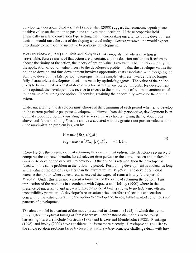
located in the sample area. Figure 2 shows the geographical relationships and a list of the major rivers/streams/creeks located in each subbasin.

Upon inspection of the data, subbasins NEU2 and NEU3 contain the areas that either have the most urbanized areas andlor have experienced rapid growth in residential development during the sample period. As published in the most recent Basinwide Assessment report by the DWQ, these subbasins are also experiencing some water quality concerns. Benthos data collected in

Figure 2 Upper Neuse River Subbasins located in Wake County

--1

Subbasin Major Rivers/Streams/Creeks

NEU 1 Ledge Cr, Beaverdam Cr, Neuse R, New light Cr, Upper Barton Cr, Lower Barton Cr

Neuse R, CrabTree Cr, Walnut Cr, Swift Cr, Smith Cr

NEU3 Middle Cr

NEU4 Black Cr

NEU6 Buffalo Cr, Little R

NEU7 Moccasin Cr

NEU2 indicate severe water quality problems. Crabtree and Swift creeks are located in this subbasin and have been reported as having elevated turbidity levels. While Smith Creek is experiencing a decline in water quality, water quality appears to be stable in this subbasin. Walnut Creek and parts of the Neuse River have shown some improvements in water quality. Elevated turbidity levels have been found in Middle Creek where the greatest development in NEU3 has occurred.

The remaining subbasins5 NEUl, NEU6, and NEU7, have experienced relatively stable water quality since the DWQ's last basinwide report. Exceptions within NEUl include New Light Creek and Upper Barton Creek. Both creeks are reported as having experienced an increase in problems f ~ o m sediments. Benthos data collected from Upper Barton Creek suggest a long-term water quality decline since 1991. The portion of Buffalo Creek located in NEU6 has also shown a decline in water quality. This decline has been attributed to the occurrence of hurricanes in the past several years. Subbasin NEU7 is reported as having excellent water quality.

MEASURES OF WATER QUALITY AND W A N DEVELOPMENT

Different sources of information can be used to assess water quality6. Data collected on physical and chemical measures, changes in benthos and fish communities, and examinations of fish tissue are all primary sources of information. To evaluate the effect of development on water quality, this analysis uses physical and chemical measures known as ambient water quality measures. Specifically, the analysis uses a single physical measure, total suspended solids (TSS) and two chemical measures, total phosphorous (TP) and total nitrogen (TN) to link development to water quality. Each pollutant is discussed in turn.

Increases in the amount of sediment entering a watershed is likely to occur as an area grows and land is moved from an undeveloped to a developed state. Erosion from construction is a harmful pollutant, clogging stream channels and water intakes. The presence of sediment increases turbidity reducing the amount of light penetration, retards photosynthesis, and hence, may lead to decreases in the food supply available to aquatic life. Sediment also interferes with the spawning of fish and may even cause respiratory organ damage. TSS is therefore thought to be a good indicator of the potential adverse effects of land conversion on water quality.

Not only do sediments directly degrade water quality, they also provide an avenue through which nutrients may enter a body of water. The absorptive properties of fine sediments coupled with the tendency of phosphorous to bind to particles makes total phosphorous another good indicator of the potential effects of development on water quality. An excess of nutrients in a body of water encourages eutrophication, which further degrades the health of the ecosystem. Phosphorous is present in streams in three different forms: (1) as soluble phosphates, (2) phosphorous bound to sediments, and (3) phosphates occurring in living organisms. Total phosphorous includes all forms of phosphorous including particulate forms and is therefore the measure used in the quantitative analysis.

Total nitrogen is the final measure used to assess the detrimental effects of land conversion on water quality. Development may cause increased levels of nitrogen in rivers and streams as sediments transport organic nitrogen into water systems. Residential development may also bring about increased fertilizer use that in turn would lead to increased levels of nitrogen from lawn runoff. Excessive levels of nitrogen encourage eutrophication and hence, damage the health of the ecosystem. Two measures of nitrogen are routinely collected by agencies interested in water quality. These measures are (1) total Kjeldahl Nitrogen (TKN) which is the sum of

5 N~ infomation is pror.ided for the poition of NEW located in Wake CountJ'. vesiland, Pierce, and Weiner (1 990) provide an excellent sumav of ~ a t ~ ~ ~ ~ / / ~ ~ j ~ ~ vavhg wdys jfl

pollution may be measured.

' ~ c h

organic nitrogen and ammonia, and (2) Nitrite + Nitrate (N+N), a form that is very mobile and easily moves with water in the soil. Organic nitrogen turns into ammonia via a process referred to as ammonification. Ammonia is a form of inorganic nitrogen that oxidizes into nitrite. Nitrite is highly unstable and quickly turns into nitrate. Thus, nitrogen is present in many different forms and is continually changing molecular form and geographical location. For this reason, a cornbined measure, total nitrogen, was used for the analysis.

GENERAL SPATIAL MODEL OF WATER QUALITY

The goal of the water quality analysis is to evaluate the effect of residential development on ambient water quality measures discussed in the previous section. In order to accomplish this goal, residential development measures must be related to pollutant readings taken at a particular point in space at a particular point in time. This task is complicated by spatial and temporal patterns in water quality that lead to space-time dependencies. For example, flow characteristics create functional relationships between what is happening upstream from a monitoring station and what is happening at the station. This type of dependency suggests the need to include a lag operator that would relate a pollutant reading taken at one point in space-time to another pollutant reading taken upstream at the immediately preceding point in time. There also are unobservable factors that affect pollutant levels. The estimated equations must include disturbance terms to account for this. These disturbance terms are likely to be correlated across space and time, which means they possess a spatial-temporal autoregressive structure. For example, county-le\~el rainfall data would not capture the differences in rainfall within the county. These unobserved differences might create correlations in the residuals between neighboring stations. As another example, the unique location of a monitoring station may affect readings, but the reasons may be unobserved. Thus, there might be correlation in the residuals at a particular station over time.

In an ideal setting, all the classical regression assumptions would hold and the linear regression model could be used:

where x denotes a vector of explanatory variables, P represents a vector of parameters to be estimated, E[u]=O, EbIx]=n-P, and u -N(o,&). For the purpose of water quality analyses, space- time dependencies exist making the above formulation inappropriate because parameter estimates would be biased as well as inefficient. Upstream neighbors are thought to influence downstream neighbors directly due to flow properties. The nature of flow implies the need to include spatially lagged dependent variables in the regression analysis. For illustration, consider a pure first order spatial autoregressive process:

where L is a spatial weights matrix for spatial lags whose elements are nonzero only for upstream neighbors, p is a spatial autoregressive coefficient, and u is an independent and identically distributed error term. Denoting Ly by yr, the OLS estimate for p is given by:

The third term in expression ( 1 5) contains a quadratic term in the errors and therefore has a nonzero expected value. This expression illustrates the bias of the OLS estimate of p in this type of setting.

An alternative fo rn of dependency may arise in the residuals. Consider the effects of an autocorrelated error term. This scenario implies Cov(uil,ujs) # 0, so again the assumptions of the classical regression model are not fulfilled. The general form of the model is given by:

where W is a spatial-temporal weights matrix that may contain nonzero elements for both spatial and temporal correlations, A is an autoregressive error coefficient, EIEil]=O, and ~ a r [ & , , ] = d . The bias of the OLS parameter estimate of p is:

Thus, OLS parameter estimates retain consistency in the presence of autocorrelated errors. Parameter estimates are, however, inefficient. The variance of POLS is:

which does not equal d ( x f x ) - * and hence, parameter estimates do not achieve minimum variance.

Employing the method of maximum likelihood to the general spatial model yields parameter estimates that exhibit consistency, asymptotic efficiency, and asymptotic normality under certain conditions. Anselin ( 1 988) discusses the conditions under which these properties hold. The conditions include: existence of a continuously differentiable log likelihood function for the parameter values under consideration; bounded partial derivatives; and a positive definite covariance matrix. The model is assumed to take the following form:

where the variables are defined as before and E - N(0,R). For ease of illustration, define A=(I- pL) and B= (I-h R'). Substituting these expressions into (16) yields:

Making the final substitution we have a model given by:

The probability distribution o fy is given by

P, (y) = det

where

det $ 1 = det 1 an1

is the Jacobian of transformation. The distribution assumption for E allows the log likelihood function to be written as:

where n is the number of observations. Expression (19) is maximized to obtain parameter estimates in a maximum likelihood framework. The first order conditions used to obtain the maximum likelihood estimates are:

These equations are nonlinear and must be solved using numerical methods.

DESCRIPTION OF THE DATA

The water quality data come from several sources. Most of the data were obtained through the North Carolina Division of Water Quality (NCDWQ). These data include observations collected directly by the NCDWQ and data provided to NCDWQ by the Lower Neuse Basin Association (LNBA). Additional data were obtained through the USGS to provide coverage for areas that were not represented by other sources. The analysis uses information on ambient water quality measures taken in Wake County and the surrounding counties. The data include total phosphorous (TP), total suspended solids (TSS), nitrite + nitrate (N+N), and total Kjeldahl nitrogen (TKN). The sample period used covers January 1995 through December 1999. Figure 3 shows the spatial location of each monitoring station. The stations in Figure 3 had at least eight months of coverage per year or when combined with another geographically close station had at least eight months of coverage.

The relationship between water quality and land use is complex. The first step in establishing a link between residential development and environmental quality is to subdivide Wake County so that each monitoring station is associated with the area of land whose drainage enters upstream from that station and below any upstream stations. Thus, flows from that land will directly affect that station's readings. A GIs hydrography data set based on the USGS 1 :24,000 scale was created by the North Carolina Center for Geographic Information and Analysis (NCCGIA) in cooperation with the North Carolina Division of Water Quality. Figure 3 contains a map of this data set. While the data set contains hydrologic areas referred to as 14-digit HUC's, these geographical units did not allow the optimal use of the data available. Some geographic units would not be represented by a monitoring station with adequate data coverage. Conversely, several hydrologic units would contain multiple stations with sufficient coverage.

Wake County was manually delineated in order to uniquely link land areas to a single monitoring station. Spatial division of Wake County was completed with the use of BASINS, a software package created and provided by the U.S.Environrnenta1 Protection Agency. BASINS 3.0 includes a manual delineation tool that allows users to subdivide watersheds into smaller hydrologically connected units. Four GIs maps were used to obtain separate land areas that could be uniquely linked to a monitoring station based on sampling coverage and the hydrologic characteristics of the area. The maps include a map of the 8-digit cataloging units located in the Neuse River Basin, a map of Wake County, the NCGIA hydrologic unit map discussed above, and a map of the major reaches in the area. All of the maps excluding the NCGIA hydrologic unit map are provided as part of BASINS.

The map of the cataloging units serves as the base map to which all boundaries were added. Two cataloging units comprising part of the Neuse River Basin are located in Wake County. These units are referred to as the Upper Neuse cataloging unit and the Contentnea cataloging unit with digit codes 03020201 and 03020203. The units were segmented into smaller watersheds using the map of Wake County, the NCCGIA hydrologic unit map, and the map of the major reaches. The map of Wake County was used to isolate the area of interest for the analysis. The NCCGIA map was used to identify smaller watersheds contained in the basin. Once these

Figure 3 Sampling sites in Wake County in the Neuse River Basin

Darker lines represent major reaches. Dots represent monitoring stations. Hydrographic delineations are based on USGS 1 :24,000 scale.

Figure 4 Wake County delineated into 24 Hydrologic Units

Darker lines represent major reaches. Dots represent monitoring stations. delineations created by manually delineating the county.

Hydrographic

boundaries were superimposed on the map containing the boundaries of the cataloging units, the land areas were either further segmented or combined with other hydrologic units based on the areas contributing to flow in a stream and sampling coverage. The map of the major reaches in the area was used to help identify these areas. By delineating in the direction of the watershed's pour point and working downstream, the map contained in Figure 4 was created. Figure 4 shows the resulting boundaries of each hydrologic unit created along with their geographical relationships to the major reaches and monitoring stations located in the area.

Comparing Figure 3 to Figure 4 one can see that the delineation process allows better use of the monitoring data by uniquely linking monitors to land areas. Table 7 provides the link between the land areas and the station numbers and locations. Along the Neuse River, areas were combined to create hydrologic units W2 and W 17. In the northeast portion of the county hydrologic unit W3 was created by combining areas represented by separate hydrologic units in Figure 3. The NCCGIA map defined one hydrologic unit to represent a large portion of the area located along Crabtree Creek. This area was divided into five separate hydrologic units: W16, W 1 1, W 14, W 13, and W 12. Hydrologic units located along Swift Creek were combined to create a larger watershed, W22. Hydrologic units located in the vicinity of Middle Creek were divided to create four hydrologic units, W7, W8, W9, and W10. Only four of the twenty-four resulting hydrologic units contained in Figure 4 are not represented by a monitoring station 7.

Tables 8-1 0 provide annual means of the ambient pollution measures for 1995 through 1999. The monitoring stations with the highest and lowest mean values for each year are in bold. Tables 1 1-1 3 aggregate over the five years and present summary statistics for each station.

Spatially delineating Wake County allowed each hydrologic unit to be linked to an exclusive area which, in turn, allowed the construction of variables intended to capture the development activity surrounding each monitoring station at the time the water quality sample was taken. Land use information collected by the Wake County Tax Assessor's office and information on housing starts provided by the U.S. Department of Commerce were used to construct a measure of development and a measure of the change in development. Total completed residential development (TOTALRES) represents the total housing stock up to the year corresponding with the year of the water quality sampling date. The housing stock was normalized by the size of the hydrologic unit measured in square kilometers.

The change in development measures the number of houses constructed in a period. The amount of development was normalized by the size of the hydrologic unit measured in square kilometers. The monthly housing starts data were used to allocate the annual development measure into monthly values. Tables 14 and 15 present the annual means for total development and change in development for each hydrologic unit. Tables 16 and 17 aggregate the years and present summary statistics for total development and change in development by hydrologic unit.

A monitoring station located directly downstream from the hydrologic unit W24 represents the unit.

28

Table 7 Hydrologic Areas and Monitoring Stations

Hydrologic Unit Monitoring Stntiorz Major River/Strenm/Creek W1 J189000 Neuse River W2 52330000 Neuse River W3 J5620000 Little River W4 52230000 Smith Creek W5 Not represented Black Creek W6 53970000 Walnut Creek W7 546 10000 Middle Creek W8 54690000 Middle Creek W9 J4870000 Middle Creek

W10 J4980000 Middle Creek W11 J32 10000 Crabtree Creek W12 53470000 Crabtree Creek W13 J3300000 Pigeon House Creek W14 J3270000,J3290000 Crabtree Creek W15 J2850000 Crabtree Creek W16 J2860000,J3000000 Crabtree Creek W17 52360000 Neuse River W18 54050000 Neuse River W19 54080000 Poplar Creek W20 Not represented Marks Creek W2 1 Not represented Buffalo Creek W22 2087580,J4414000 Swift Creek W23 Not represented Whiteoak Creek W24 56500000 Moccasin Creek

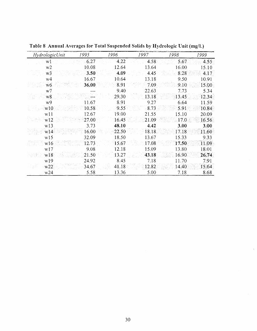
Table 8 Annual Averages for Total Suspended Solids by Hydrologic Unit (mg/L) -

Hvdroloaic Un it 1995 1996 1997 1998 1999

w l l 12.67 19.00 21.55 15.10 20.09 w12 27.00 16. w13 3.73 48.10 4.42 3.00 3.00

Table 9 Annual Averages for Total Phosphorous by Hydrologic Unit (mglL)

w l l 0.29 0.23 0.23 0.06 0.09

Table 10 Annual Averages for Total Nitrogen by Hydrologic Unit (mg/L)

Hydrologic Unit 1995 1996 1997 1998 1999 wl 0.61 0.59 0.5 1 0.42 ---

w l l 3.25 1.87 1.03 0.63 1.08 .02

Table 1 1 Summary Statistics for Total Suspended Solids by Hydrologic Unit (mg/L)

Hydrologic C h it N Mean media^^ Std Dev Min 12.lr,,x

W1 55 5.0910 5 .OO 2.8692 1.00 13.00 W2 55 13.3842 1 1 .OO 9.6374 0.06 46.00 W3 57 4.8607 4.00 4.72 13 0.01 28.00 W4 55 12.3 100 7.00 16.4927 0.01 79.00 W6 55 15.7104 5.00 30.481 1 0.01 177.00 W7 44 11.1839 5.50 22.0552 0 146.00 W8 44 16.6825 8.50 27.7625 0.01 164.00 W9 57 9.6854 6.00 10.8323 0.01 54.00

W10 57 9.1763 7.00 8.1912 0.01 41.00 W11 55 17.6369 12.00 23.6767 0.01 135.00 W12 55 19.8033 12.00 28.8642 0.02 150.00 14713 56 11 SO00 2.00 57.1082 0 430.00 W14 48 17.6667 10.00 19.8294 1.00 100.00 W15 57 17.5088 15 .OO 13.0864 1.00 67.00 W16 56 14.91 07 7.00 19.9018 1.00 96.00 W17 55 13.5476 10.00 12.5863 0.05 62.00 W18 55 24.40 16 11 .OO 52.9327 0.04 380.00 W19 55 12.2733 6.00 21.8413 0.01 147.00 W22 55 24.1098 7.00 53.201 1 0.01 339.00 W24 57 7.93 18 5.00 13.3376 0.01 97.00 Wake 1083 13 .9060 7.00 27.5215 0 430.00

Table 12 Summary Statistics for Total Phosphorous by Hydrologic Unit (mg/L)

Hydvo/ogic Unit N Median Std Dev Min A lux W1 W2 W3 W4 W6 W7 W8 W9

W10 W11 W12 W13 W13 W15 W16 W17 W18 W19 W22 W24 Wake

Table 13 Summary Statistics for Total Nitrogen by Hydrologic Unit (mg/L)

Hydrologic N hfea 71 Median Std Dev Ilfilz M a x U?lit w 1 W2 W3 W4 W6 W7 W 8 W9 Llr 10 W11 W12 W13 W14 W15 W16 W17 W18 W19 W22 W24 Wake

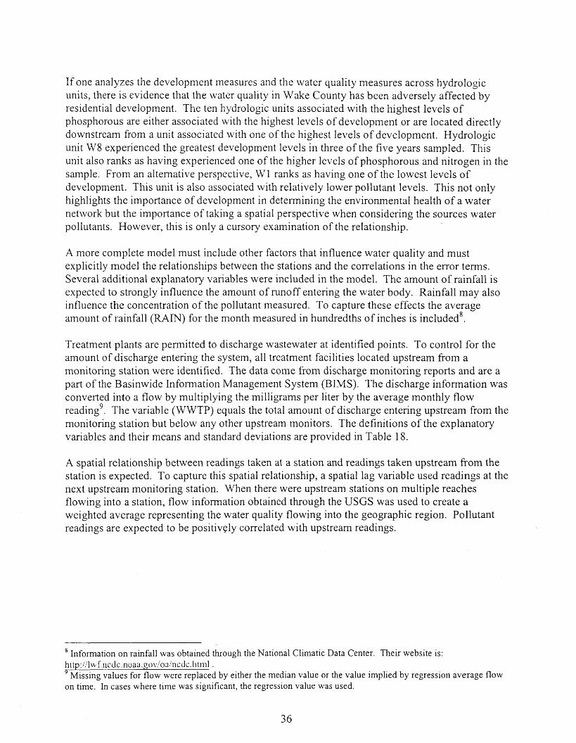
If one analyzes the development measures and the water quality measures across hydrologic units, there is evidence that the water quality in Wake County has been adversely affected by residential development. The ten hydrologic units associated with the highest levels of phosphorous are either associated with the highest levels of development or are located directly downstream from a unit associated with one of the highest levels of development. Hydrologic unit W8 experienced the greatest development levels in three of the five years sampled. This unit also ranks as having experienced one of the higher levels of phosphorous and nitrogen in the sample. From an alternative perspective, W 1 ranks as having one of the lowest levels of development. This unit is also associated with relatively lower pollutant levels. This not only highlights the importance of development in determining the environmental health of a water network but the importance of taking a spatial perspective when considering the sources water pollutants. However, this is only a cursory examination of the relationship.

A more complete model must include other factors that influence water quality and must explicitly model the relationships between the stations and the correlations in the error terms. Several additional explanatory variables were included in the model. The amount of rainfall is expected to strongly influence the amount of runoff entering the water body. Rainfall may also influence the concentration of the pollutant measured. To capture these effects the average amount of rainfall (RAIN) for the month measured in hundredths of inches is included8.

Treatment plants are permitted to discharge wastewater at identified points. To control for the amount of discharge entering the system, all treatment facilities located upstream from a monitoring station were identified. The data come from discharge monitoring reports and are a part of the Basinwide Information Management System (BIMS). The discharge information was converted into a flow by multiplying the milligrams per liter by the average monthly flow reading9. The variable (WWTP) equals the total amount of discharge entering upstream from the monitoring station but below any other upstream monitors. The definitions of the explanatory variables and their means and standard deviations are provided in Table 18.

A spatial relationship between readings taken at a station and readings taken upstream from the station is expected. To capture this spatial relationship, a spatial lag variable used readings at the next upstream monitoring station. When there were upstream stations on multiple reaches flowing into a station, flow information obtained through the USGS was used to create a weighted average representing the water quality flowing into the geographic region. Pollutant readings are expected to be positively correlated with upstream readings.

Information on rainfall was obtained through the National Climatic Data Center. Their website is: h ~ t p : ~ / l ~ ~ f . ~ ~ c d c . n o a a . g ~ ~ ~ ~ ~ ~ ~ ~ n ~ d ~ . l : t ~ ~ ~ l .

Missing values for flow were replaced by either the median value or the value implied by regression average flow on time. In cases where time was significant, the regression value was used.

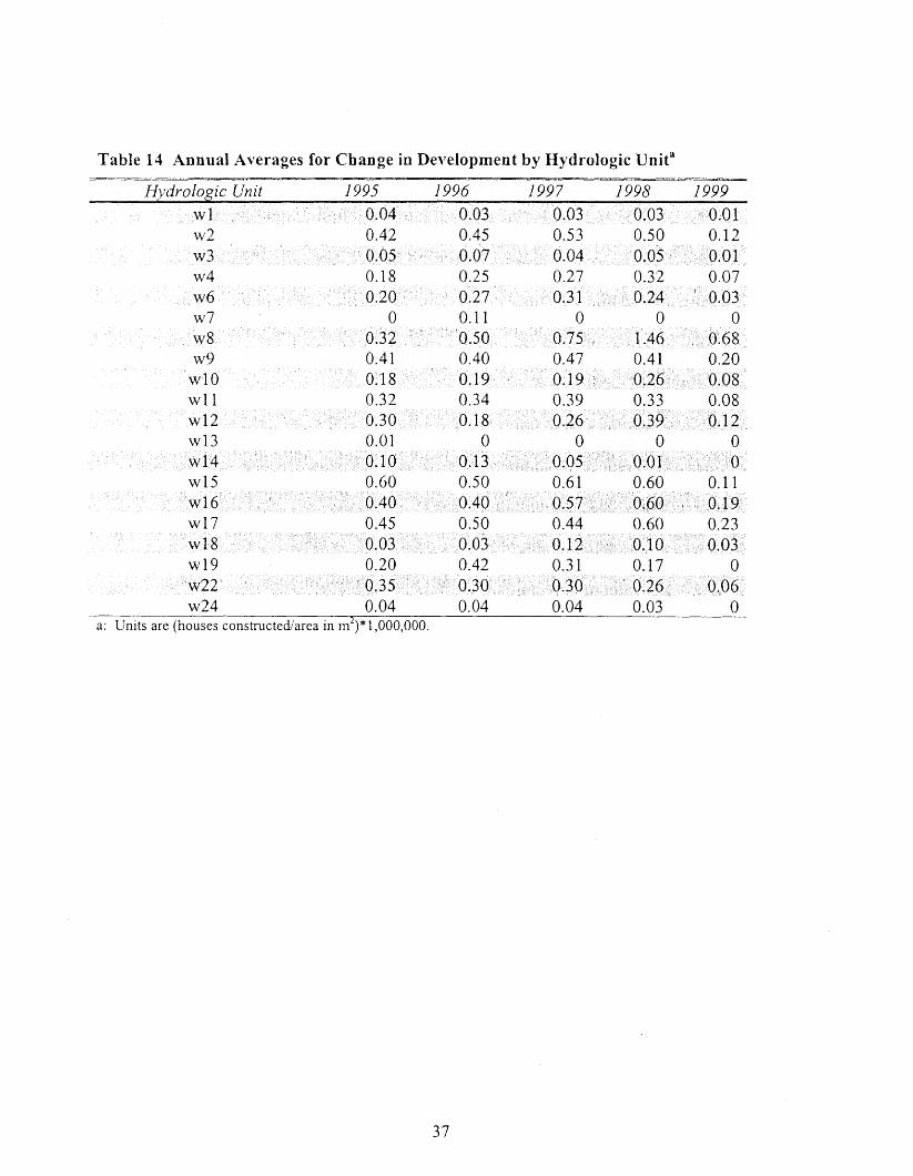
Table 14 Annual Ayerages for Change in Development by Hydrologic Unita

Hydrologic Unit 1995 1996 1997 1998 1999 w l 0.04 0 -03 0.03 0.03 0.0 1

w6 0.20 0.27 0.3 1 0.24 0.03

w10 0.18 0.19 0.19 0.26 0.08

w24 0.04 0.04 0.03 0 a: Units are (houses constructed/area in m2)* 1,000,000.

Table 15 Annual Averages for Total Development by Hydrologic unitb

Hydrologic UII it 1995 1996 1997 1998 1999 w l 2.3 2.7 3.1 3.4 3.7

w l l 228.1 236.4 240.6 243.5

62.4 63.7 73.9 80.1 85.7

w24 16.3 16.8 17.3 17.8 18.0 b: Units are (total housing stocWarea in m2)* 1,000,000.

Table 16 Summary Statistics for the Change in Development by Hydrologic Unita --- - -

~ j ) d & l ogic unit N Meal-1 Median Std Dev Min Max

I

a: Units are (houses constructed/area in m2)* 1,000,000.

W1 W2 UT3 W4 W5 W6 W7 W8 W9

W10 W11 W12 W13 W14 W15 W16 W17 W18 W19 W20 W2 1 W22 W23 W24 Wake

Table 17 Summary Statistics for Total Residential Development by Hydrologic unitb

Hydrologic Unit N Mean Median Std Dev Min M& W l W2 W3 W4 W5 W6 LV 7 W8 W9

W10 W l 1 W12 W13 W14 W15 W16 W17 W18 W19 W20 W2 1 W22 W23 W24 Wake

b: Units are (total housing stocWarea in mZ)* 1,000,000.

Table 18 Variable Definitions and Summary Statistics

Variable Definition Mean Std. Dev.

TOTALRES Total housing stock per square kilometer 92.53 85.20

DEV

RAIN

Monthly change in the total housing stock 0.25 0.24 per square kilometer

Average amount of monthly rainfall in 407.54 302.44 hundredths of inches

WWTP - TN Point-source discharge of TN 0.13 0.40 entering upstream from a monitoring station (measured in (mg/L)*mgd)

WWTP-TP Point-source discharge of TP 0.0 1 entering upstream from a monitoring station (measured in (mg/L)*mgd)

WWTP - TSS Point-source discharge of TSS 1.18 4.23 entering upstream from a monitoring station (measured in (mg/L)*mgd)

ECONOMETRIC RESULTS

The general spatial model allowing for spatial lags and correlated errors was run for each of the three pollutants. Results are reported in Table 19. The model appears to explain approximately 39% of the variation in the log of total nitrogen (TN), 39% of the variation in the log of total phosphorous (TP), and 15% of the variation in the log of total suspended solids (TSS). As expected, residential construction appears to adversely affect water quality with respect to each of the pollutants. The estimates are positive and statistically significant in all cases. New development appears to have a larger effect on TP than TN. This finding is expected given the tendency of phosphorous to bind to particles. Construction would directly increase the amount of sediment entering a body of water and consequently increase the avenues through which phosphorous may enter the system. The density of housing also has a positive and significant effect on TP and TN. While the parameter estimate for the effect of housing density on TSS is negative, the estimate is not statistically significant. This is to be expected. While runoff from construction sites would affect TSS, once the lots are developed there is probably less impact on that pollutant.

As expected, the amount of wastewater entering upstream from a station appears to be positively correlated with pollutant readings taken at a station. Results for the spatial relationships are given by RHO and LAMBDA. Spatial effects appear to be strongly significant. RHO is the parameter estimate for the spatially lagged dependent variable. The lagged dependent variable equals the sum of the upstream pollutant readings when neighboring stations exist and 0 ~ t h e n v i s e ' ~ . Each reading in the sum is weighted by its relative flow. The estimate of RHO indicates that pollutant readings are positively correlated with upstream readings. The relationship is less than unity, as would be expected because of in-stream loss. LAMBDA is the autoregressive error coefficient. This parameter captures the temporal correlation in the errors. Observations taken in period T are related to observations taken in period T-1 and T+l for the same station. The results indicate that the errors are positively correlated with readings taken in preceding and subsequent time periods.

One can use the coefficients on TOTALRES and DEV to determine the impact of urban residential development on water quality within Wake County. In spite of the maximum likelihood estimation of the spatial econometric specification, the interpretation of the coefficients is closely related to the interpretation in semi-logarithmic regressions. The natural logarithm of the pollutant reading (TN, for example) is explained by the levels of the explanatory variables:

Taking the anti-log of both sides of the equation implies that the pollutant reading equals the exponential of the estimated equation:

'O It seemed appropriate to assign zero for stations that had no upstream station because they are typically near the headwaters and the associated hydrologic unit includes most of the sources of pollution affecting that station.

Table 19 General Spatial Iklodel Estimates - - -

TN Parameter TP Parameter Variable

TSS Param eter Estimates Estimates Esfit~~ates

Intercept

TOTALRES

DEV

WWTP

RHO

LAMBDA

N 1036 1036 1043 Rbar-Square 0.3936 0.3938 0.1522

Dependent Variable: ln(pol1utant); T-statistics are in parentheses.

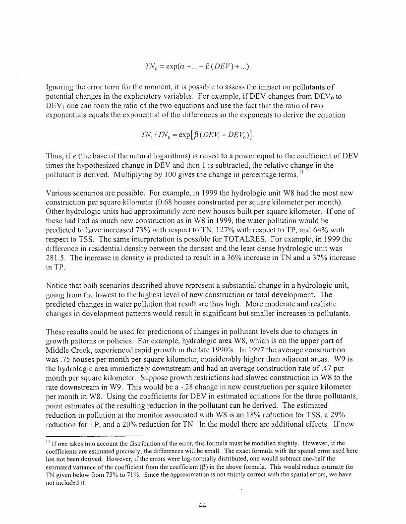
TNo = exp(a +... + p (DEV) +...)

Ignoring the error term for the moment, it is possible to assess the impact on pollutants of potential changes in the explanatory variables. For example, if DEV changes from DEVo to DEV, one can form the ratio of the two equations and use the fact that the ratio of two exponentials equals the exponential of the differences in the exponents to derive the equation

TN, / TN, = exp [ P (DE V, - DE L~~)].

Thus, if e (the base of the natural logarithms) is raised to a power equal to the coefficient of DEV times the hypothesized change in DEV and then 1 is subtracted, the relative change in the pollutant is derived. Multiplying by 100 gives the change in percentage terms."

Various scenarios are possible. For example, in 1999 the hydrologic unit W8 had the most new construction per square kilometer (0.68 houses constructed per square kilometer per month). Other hydrologic units had approximately zero new houses built per square kilometer. If one of these had had as much new construction as in W8 in 1999, the water pollution would be predicted to have increased 73% with respect to TN, 127% with respect to TP, and 64% with respect to TSS. The same interpretation is possible for TOTALRES. For example, in 1999 the difference in residential density between the densest and the least dense hydrologic unit was 281.5. The increase in density is predicted to result in a 36% increase in TN and a 37% increase in TP.

Notice that both scenarios described above represent a substantial change in a hydrologic unit, going from the lowest to the highest level of new construction or total development. The predicted changes in water pollution that result are thus high. More moderate and realistic changes in development patterns would result in significant but smaller increases in pollutants.

These results could be used for predictions of changes in pollutant levels due to changes in growth patterns or policies. For example, hydrologic area W8, which is on the upper part of Middle Creek, experienced rapid growth in the late 1990's. In 1997 the average construction was .75 houses per month per square kilometer, considerably higher than adjacent areas. W9 is the hydrologic area immediately downstream and had an average construction rate of .47 per month per square kilometer. Suppose growth restrictions had slowed construction in W8 to the rate downstream in W9. This would be a -.28 change in new construction per square kilometer per month in W8. Using the coefficients for DEV in estimated equations for the three pollutants, point estimates of the resulting reduction in the pollutant can be derived. The estimated reduction in pollution at the monitor associated with W8 is an 18% reduction for TSS, a 29% reduction for TP, and a 20% reduction for TN. In the model there are additional effects. If new

" If one takes into account the distribution of the error, this formula must be modified slightly. However, if the coefficients are estimated precisely, the differences will be small. The exact formula with the spatial error used here has not been derived. However, if the errors were log-normally distributed, one would subtract one-half the estimated variance of the coefficient from the coefficient (0) in the above formula. This would reduce estimate for TN given below from 73% to 71%. Since the approximation is not strictly correct with the spatial errors, we have not included it.

construction is reduced this year, the housi~lg stock is reduced next year. However, a reduction in new construction by .28 per month would only result in a decrease in TOTALRES next year by about 3-113 units per square kilometer. The impact of such a change on the pollutant in subsequent years would be less than a 1% reduction in any of the pollutants. However, reducing pollutants from construction in W8 also influences pollution downstream. Using the coefficient on the spatial lag, W9 could be predicted to experience about a 6% reduction in TSS and TN and a 2.3% reduction in TP. Stations further downstream would also experience reductions, but the effects would decay fairly rapidly with distance

It is possible to compare the estimated impacts of changes in urban residential development and use on water quality to the impacts from changes in discharges from point-source wastewater treatment facilities. For this comparison to be meaningful, the impacts must be expressed in comparable terms. Once again, elasticities are useful here. Elasticities can be thought of as the percentage change in the pollutant measure divided by the percentage change in the variable affecting the pollutant. An alternative way of thinking about an elasticity is the percentage change in the pollutant resulting from a one percent change in the variable affecting the pollutant. With the specification in the general spatial model estimated here, this elasticity is calculated as the product of the estimated coefficient and the value of the explanatory variable. Thus it depends on the specific value of the explanatory variable that is used. Table 20 gives the elasticities calculated at the mean of the explanatory variable. If total existing residential development were one-percent higher, the expected increase in TN and TP would be about one- tenth of a percent. If new construction were one-percent higher, the expected increase in the each of the pollutants ranges from just under two-tenths of a percent (TSS) to just over three- tenths of a percent (TP). On the other hand, a one-percent increase in wastewater treatment plant discharges would result in much smaller increases, ranging from 2 one-thousandths of a percent for TSS to 3 one-hundredths for TN. This result seems surprising at first glance. However, controls on point sources have been in place for years and have realized substantial reductions. A one-percent increase in effluents from point sources will have a smaller impact on water quality than a one-percent increase from nonpoint sources if the nonpoint sources account for a larger fraction of the pollutants entering the waterway. In designing policies to deal with these types of water pollutants, urban residential development and use are important factors. A one- percent change in these factors would have about ten times the impact on pollution when compared to a one-percent change in point-source pollution.

Table 20 Pollutant elasticities with respect to explanatory variables

Variable TN TP TSS

TOTALRES 0.102 0.102 ---

DEV 0.201 0.303 0.183

WWTP 0.030 0.015 0.002

This analysis of hypothetical changes in urban development illustrates the power of the spatially dynamic models that can be estimated. However, the results are only illustrative and should not be interpreted as evidence of the need to limit urban growth. Rather, they illustrate the importance of developing ways to reduce urban runoff. Limiting development is only one method and is perhaps not the most desirable.

SUMMARY AND CONCLUSIONS

This study provides strong evidence of the effects of urban residential construction and land use on water quality and the factors that influence here that land use change takes place.

\+%ere and when urban development takes place has been studied using an optimal stopping model involving a series of discrete binary choices and alternatively using a proportional hazard model. Each model has identified a number of factors that significantly influence when a parcel is developed. Among these we find that the surrounding residential activity, particularly contemporaneous development activity, is important in explaining why an individual parcel is developed in a given year. Related to this, incorporation into a n~unicipality signals that development of a parcel is more likely, due in part to the increased availability of sewer and other services. Interpolating from these two findings suggests that, all else being equal, development follows development as a critical mass of existing residential density and development activity increases the attractiveness of vacant plots for residential use. The development likelihood is further augmented if the parcel has good access to employment centers such as RTP. From this we can speculate that improved infrastructure for commuting to e~nployment (and perhaps amenity and service) areas increases the attractiveness of a parcel for residential use. Thus we would expect greater future development in areas with improved transportation infrastructure.

The effects of this development on water quality have been studied using a unique data set and spatial econometric techniques. The upper Neuse h v e r basin in Wake County, North Carolina was delineated into drainage zones such that water quality in each zone was consistently monitored for total phosphorous (TP), total nitrogen (TN), and total suspended solids (TSS) between 1995 and 1999. Data on when each residential parcel was developed were used to develop measures of the residential development and change in development for each zone. Measures of discharges from wastewater treatment plants upstream from each monitor were developed. In-stream transport of pollutants was measured, as well as other variables. These data were then used in a spatially autoregressive model. The ~esul ts indicate that both total residential development and changes in that development have statistically significant positive effects on TP and TN, while only new construction affects TSS. The other variables perform as expected. The impacts of changes in the residential variables have proportionally much larger effects than changes in point-source discharges.

This study has demonstrated that careful statistical analysis of water quality issues at a disaggregated geographical scale can be informative in numerous dimensions. In particular, we are able to isolate the impact that residential land use and new residential development have on ambient water quality measures. Because these variables are found to negatively impact water quality, we conclude that urban water quality regulation needs to consider the impact of the location and timing of residential land use and land development. We caution, however, that residential land use is far from the only factor influencing urban water quality, suggesting that water quality policy should not focus on land use regulation to the exclusion of other sources.

Our findings suggest a few paths for additional investigation to refine and corroborate our conclusions. This study has used two commonly monitored chemical measures and one physical

measure to represent the potential water quality effects of urban development. It would be interesting to do similar research with other pollutants and other measures of river basin health (e.g., benthic macroinvertibrates). It would also be interesting to reduce the geographic scale still further, allowing investigation of water quality impacts at the neighborhood rather than hydrological unit level. Finally, studying the effects of development on water quality in areas with different soil types, etc. would be useful. All these research efforts will depend on more extensive water quality n~onitoring, particularly in areas predicted by our development model to see increasing development activity.

This development model could be used in addressing a variety of policy issues linking water quality and land use. These policies may be designed to influence the location of development, the nature of development, or the mitigating steps taken during development. With additional refinements, it may be possible to predict changes in water quality resulting from proposed policies.

Further improvements in the estimation are possible. For example, simultaneous estimation of the equations for the three pollutants would allow for correlated errors across equations. With spatial autocorrelation this is still possible, although it is more complex that the usual seemingly unrelated regression model. Refining the models of the development decision will allow better forecasts for urban growth so that ecological vulnerability can be considered and policies designed. An important step will be to incorporate spatially and temporally correlated unobserved factors.

REFERENCES

Alonso, W, 1964 Location and Land Use. Cambridge, M A : Harvard University Press.

h a s , A., 1992. On the birth and growth of cities: Laissez-Faire and Planning Compared. Regional Science Urban Economics. 3 1 : 164- 1 SO.

Anas, A., R. Arnott, and K. Small, 1998. Urban Spatial Structure. Journal ofEconomic Literature. 36: 1426-1 464.

Anas, A., and I. Kim, 1996. General equilibrium models of polycentric urban land use with endogenous congestion and job agglomeration. Journal of Urban Economics. 40:232- 256.

Anselin, L. and R. J. Florax, 1995. eds. New Directions in Spatial Econometrics. New York: Springer Verlag, 1995.

Anselin, L., 1988. Spatial Econometrics: Methods and Models, Dorddrecht: Kluwer Academic Publishers.

Arnott, R., and F. Lewis, 1979. The transition of land to urban use. Journal ofPolitica1 Econorny. 87: 161-169.

Arrow, K.J., and A. C. Fisher, 1974. Environmental preservation, uncertainty, and Irreversibility. Quarterly Journal of Economics. 88:3 12-3 1 9.

Brazee, R., and R. Mendelsohn, 1988. Timber harvesting with fluctuating prices. Forest Science. 34:359-372.

Bockstael, N.E., 1996. Modeling economics and ecology: the importance of a spatial Perspective. American Journal of Agricultural Economics. 78: 1 168- 1 1 80.

Campolieti, M. 2000. Bayesian estimation and smoothing of the baseline hazard in discrete time duration models, Review ofEconomics and Statistics. 82:685-701.

Capozza, D. and R. Helsley, 1989. The Fundamentals of land prices and urban growth. Journal of Urban Economics. 26:295-306.

Capozza, D. and R. Helsley, 1 990. The Stochastic city. Journal of Urban Economics. 28: 1 87- 203.

Capozza, D. and Y. Li, 2002. Optimal land development decisions. Journal o furban Economics. 5 1 : 123-142.

Chiew F.H.S. and R.A. McMahon. Modeling runoff and diffuse pollution loads in urban areas. Water Science and Technology. 39:241-248.

Cox, D., 1972. Regression models and life-tables (with discussion). Journal of the Royal Statistical Society, Series B. 34: 187-220.

Cox, D., 1975. Partial Likelihood. Biometrika, 62, 269-276.

DeLong, D., G. Guirguis, and 1'. So, (1 994). Efficient computation of subset selection probabilities with application to Cox regression. Biometrika. 8 1 :607-611.

Division of Water Quality, 2001. Businwide ..lssess?nent Report: Neuse River Basin. North Carolina Department of Environment and Natural Resources.

Dixit, A. and R. Pindyck, 1994. Investment Under Uncertainty. Princeton, NJ: Princeton University Press.

Dubin, R., 1995. "Estimating logit models with spatial dependence", in Anselin, L., and Florax, R.J., New Directions in Spatial Econometrics, New York: Springer Verlag.

Efron, B, (1977). The efficiency of Cox's likelihood function for censored data. Journal of the American Statistical Associution. 7237-565 .

Fisher, A.C., 2000. Investment under uncertainty and option value in environmental economics. Resource and Energy Economics. 22: 197-204.

Goovaerts, P., 1997. Geostatistics for natural resources evaluation. New York: Oxford University Press.

Gumpertz, M.L., C. T. Wu, and J. M. Pye, 2000. Logistic regression for southern pine beetle outbreaks with spatial and temporal autocorrelation. Forest Science. 46:95-107.

Hoynes, H., 2000. Local labor markets and welfare spells: Do demand conditions matter? Review of Economics and Statistics. 82:35 1-368.

Henry, C., 1974. Investment decisions under uncertainty: the irreversibility effect. American Economic Review. 64: 1006-101 2.

Hunsaker, C.T., and Levine, D.A., 1995. Heirarchical approaches to the study of water in rivers. Bioscience 45 : 193-203.

Insley, M., 2002. A real options approach to the valuation of forestry investment. Journal of Environmental Economics and Management. 44:426-447.

Irwin, E., and K. Bell, 2002. "Modeling and managing urban growth at the rural urban fringe evidence from residential land use change in central Maryland",forthcoming in Bell, K., Boyle, K., Plantiga, A., Rubin, J., and Tersil, M., The Economies ofLand Use Change, Ashgate Press.

Irwin, E., and N. E. Bockstael, 2002. Interacting agents, spatial externalities, and the edogenous of residential land use patterns. Journul ofEco~ornicGeogrupl?y. 2:3 1-54.

Irwin, E., and N. E. Bockstael, 2001. The problem of identifying land use spillovers: measuring the effects of open space on residential property values. Forthcoming in American Journal ofAgricultural Econonlics.

Kahn, A.E., 1966. The Tyranny of small decisions: Market failures, imperfections, and the limits of economics. KYKLOS. 19:23-45.

Keifer, N., 1988. Econon~ic duration data and hazard functions. Journal of EconomicLiterature. 26:646-679.

Keifer, N., S. Lundberg, and G. Neumann, 1985 How long is a spell of unemployment? Illusions and biases in the use of CPS data. Journal ofBusiness & Economic Statistics. 3: 118-128.

Lancaster, T., 1990. The Econometric Analysis of Transition Data. New York: Cambridge University Press.

Mills, E., 1967. An aggregative model of resource allocation in a metropolitan area. American Economic Review: 57: 197-2 10.

Moulton, B.R., 1990. An illustration of a pitfall in estimating the effects of aggregate on micro units. Review ofEconomics and Statistics, 72:334-338.

Muth, R., 1969. Cities and Housing. Chicago: The University of Chicago Press.

Norstrom, C.J., 1975. A stochastic model for the growth period decision in forestry. Swedish Journal of Economics. 77:329-337.

Palmquist, R.B., 1989. Land as a differentiated factor of production: A hedonic model and its implications for welfare measurement. Land Economics 65, 23-28.

Papageorgiou, Y., and T. Smith, 1983. Agglomeration as local instability in spatially uniform steady-states. Econometrics. 5 1 : 1 109- 1 1 19.

Pindyck, R.S., 1991. Irreversibility, uncertainty, and investment. Journal ofEconomic Literature. 29: 1 1 10- 1 152.

*

Plantinga, A.J., 1998. The optimal timber rotation: an option value approach. Forest Science. 44: 192-202.

Rosen, R., 1974. Hedonic prices and implicit markets: product differentiation in pure competition. Journal of Political Economy. 8 2 % - 5 5 .

Smith, R.A., G. E. Schwarz, and R. B. Alexander, 1997. Regional interpretation of water quality monitoring data. Water Resources Research. 33 :278 1-2798.

Thornson, T.A., 1992. Optimal forest rotation when stumpage prices follow a diffusion process. La~td Economics. 68:329-342.

Vesilind, P.A., J. J. Peirce, and R. F. Weiner, 1990. Environmental Pollution and Control, Butterworth-Heinemann.

Wang, X. and 2. Ying, 1997. Using GIs to assess the relationship between land use and water quality at a watershed level. Environmental International. 23 : 103- 1 14.

White, M., 1976. Firm suburbanization and urban subcenters. Journal of Urban Economics. 3:323-343.

White, M., 1988. Location choice and commuting behavior in cities with decentralized employment. Journal of Urban Economics. 24: 129- 152.

Wieand, K., 1987. An extension of the monocentric urban spatial equilibrium model to a multicenter setting: The case of the two-center city. Journal of Urban Economics. 2 1 :259-27 1.