LAMINAR LIQUID-LIQUID DISPERSION IN SMX STATIC MIXER · In this research, liquid-liquid dispersion...
90
LAMINAR LIQUID-LIQUID DISPERSION IN SMX STATIC MIXER
Transcript of LAMINAR LIQUID-LIQUID DISPERSION IN SMX STATIC MIXER · In this research, liquid-liquid dispersion...

LAMINAR LIQUID-LIQUID DISPERSION IN SMX STATIC MIXER

STUDY OF LIQUID-LIQUID DISPERSION OF HIGH VISCOSITY FLUIDS IN SMX
STATIC MIXER IN THE LAMINAR REGIME
By
MAINAK DAS, B.Sc. Eng.
A Thesis
Submitted to the School of Graduate Studies
in Partial Fulfillment of the Requirements
for the Degree
Master of Applied Science
McMaster University
©Copyright by Mainak Das, September 2011

ii
MASTER OF APPLIED SCIENCE (2011) McMaster University
(Chemical Engineering) Hamilton, Ontario
TITLE: Study of Liquid-Liquid Dispersion of High Viscosity
Fluids in SMX Static Mixer in the Laminar Regime
AUTHOR: Mainak Das, B.Sc.Eng. (University of Alberta)
SUPERVISORS: Dr. Andrew N. Hrymak and Dr. Malcolm H.I. Baird
NUMBER OF PAGES: xiii, 67, A4, B3

iii
Abstract
In this research, liquid-liquid dispersion of viscous fluids was studied in an
SMX static mixer in the laminar regime. Backlighting technique was used for
flow visualization, and the Hough transform for circle detection was used in
OpenCV to automatically detect and measure drop diameters for obtaining the
size distribution. Silicone oil and an aqueous solution of high fructose corn syrup
were used for dispersed and continuous phases respectively, and sodium
dodecyl sulfate was used as the surfactant to modify the interfacial tension.
Experiments were conducted at varying viscosity ratios and flow rates-each at
zero, low (~200 ppm) and high (~1000 ppm) surfactant concentrations. The
effect of holdup was explored only for a few cases, but it was found to have a
minimal effect on the weighted average diameter D43.
It was found that the superficial velocity and the continuous phase
viscosity had a dominant effect on D43. The tail at the higher end of the droplet
size distribution decreased with increasing superficial velocity and continuous
phase viscosities. It was also found that D43 decreased with lowering of the
interfacial tension. Furthermore, the effect of the dispersed phase viscosity was
significant only at non zero surfactant concentrations.
An approximate model has been proposed that relates D43 to the capillary
number. It is based on an energy analysis of the work done by the viscous and

iv
surface forces on a drop of an initial diameter that is largely determined by the
gap distance between the cross bars in the element.

v
Acknowledgements
I would like to sincerely express my gratitude to Dr. Hrymak and Dr. Baird
for giving me this learning opportunity and guiding me throughout this project.
Their commitment to the success of this research and innovative problem solving
approaches has been truly inspirational.
I would like to thank Paul Gatt and Dan Wright for helping with
equipment setup and troubleshooting. Their on-demand help made it possible
to finish this project on time. I would also like to thank Justyna Derkach for
providing guidance and assistance with lab safety.
My sincere thanks goes to Dr. Pelton`s group (especially Yuguo Cui) for
providing access to their equipments. Also, I would like to thank my colleagues
and friends for exchanging valuable information.
I would also like to acknowledge the financial support from the
Department of Chemical Engineering and School of Graduate Studies by
providing scholarships and teaching assistantships. I am also grateful to Proctor
& Gamble for funding this project.
Lastly, I would like to thank my parents and other family members for
their encouragement and constant support.

vi
Table of Contents
Abstract iii
Acknowledgements v
Table of Contents vi
List of Figures viii
List of Tables xi
Nomenclature xii
1. Introduction 1
2. Literature Review 5
2.1 Drop breakup 5
2.2 Correlations in the laminar regime 11
2.3 Correlations in the turbulent regime 15
2.4 Automated droplet detection 19
3. Experimental 25
3.1 Fluids used 25
3.2 Experimental rig and procedure 26
3.3 Flow visualization setup and image capture 31

vii
3.4 Image processing and circle detection 32
3.5 Note on measurement errors 38
4. Results and Discussion 40
4.1 D43 trends 40
4.2 Dmax trends 47
4.3 Droplet size distribution trends 49
4.4 Qualitative Images 55
5. Conclusion 62
5.1 Summary 62
5.2 Recommendations for future work 64
References 65
Appendix A A1
Appendix B B1

viii
List of Figures
Figure 1. Stability curves relating critical capillary number
with the viscosity ratio 6
Figure 2. Critical Capillary number as a function of viscosity ratio for three
different values of 8
Figure 3. Drop breakup modes in shear flow 9
Figure 4. Break up modes 10
Figure 5. Effective shear rate for SMX and Kenics mixe 13
Figure 6. 3D parameter space in standard Hough Transform for
circle detection 21
Figure 7. Two stage Hough transform illustration 22
Figure 8. Voting window 23
Figure 9. Process flow diagram with instrumentation 28
Figure 10. Entry configurations for continuous and dispersed phases 30
Figure 11. Flow visualization setup 32
Figure 12. Flow chart for image processing code 33
Figure 13. Sample raw image 34
Figure 14. Image after Bilateral Smoothing 35
Figure 15. Binary image after Canny Edge detection 36
Figure 16. Identified droplets 37

ix
Figure 17. Log-log plot to show the effect of interfacial tension
and viscosity ratio on D43 for c ~25 mPaS 41
Figure 18. Log-log plot to show the effect of interfacial tension
and viscosity ratio on D43 for c ~70mPaS 42
Figure 19. Log-log plot to show the effect of interfacial tension
and viscosity ratio on D43 for c ~200 mPaS 42
Figure 20. Log-log plot to show the effect of viscosity ratio on D43 at zero
surfactant concentration 44
Figure 21. Log-log plot to show the effect of viscosity ratio on D43 at low
surfactant concentration 45
Figure 22. Log-log plot to show the effect of viscosity ratio on D43 at high
surfactant concentration 45
Figure 23. Effect of number of elements on D43 46
Figure 24. Effect of interfacial tension and viscosity ratio on Dmax
for c ~25 mPaS 47
Figure 25. Effect of interfacial tension and viscosity ratio on Dmax
for c ~70 mPaS 48
Figure 26. Effect of interfacial tension and viscosity ratio on Dmax
for c ~200 mPaS 48
Figure 27. Image showing the breakup of a dispersed phase stream into drops as
it is passes through the gap between the cross bars 56

x
Figure 28. Image sequence showing drop breakup from impact with cross-points
of the packing 56
Figure 29. Image sequence showing a single drop breakup at cross-point 57
Figure 30. Model assessment by correlating D43 with capillary number 60

xi
List of Tables
Table 1. Correlations for droplet diameter in static mixers
in the turbulent regime 18
Table 2. Properties of fluids used in experiments 25
Table 3. Relative errors of measured and calculated values 38
Table 4. Droplet size distribution trends at zero surfactant concentration 50
Table 5. Droplet Size Distribution Trends at High Surfactant Concentration 53

xii
Nomenclature
Ca capillary number
Cacrit critical capillary number
CoV coefficient of variation
D mixer diameter, m
D0 drop primary diameter, m
D16 diameter below which 16% of the droplets lie in a distribution, m
D32 sauter mean diameter, m
D43 volume mean diameter, m
D84 diameter below which 84% of the droplets lie in a distribution, m
D90 diameter below which 90% of the droplets lie in a distribution, m
Df final droplet diameter after breakup of a primary drop, m
Di diameter of an individual drop in a distribution, m
Dmax maximum diameter, m
E overall energy, J
LT large turbulence scale, m
N number of droplets formed after break
n number of mixing elements
N0 number of droplets with an initial diameter D0
p viscosity ratio (dispersed to continuous phase)
Q volumetric flow rate, m3/s
r drop radius, m

xiii
Re Reynolds number
u superficial velocity, m/s
Vi viscosity group
Volmixer mixer volume, m3
We Weber number
P pressure drop across the mixer, Pa
Greek Letters
shear rate, s-1
flow parameter
power dissipation per unit mass, m2/s3
dispersed phase volume fraction
Kolmogorov scale, m
viscosity, Pa.S
density, kg/m3
interfacial tension, N/m
shear stress, Pa
Subscripts
c continuous phase
d dispersed phase
e emulsion
h hydraulic
p pore

M.A.Sc. Thesis - M. Das McMaster - Chemical Engineering
1
1. Introduction
Motionless mixers or static mixers have been in use since the 1970’s (Thakur
et al., 2003), and with time they have evolved to the point where they are now
found in a wide array of industries. These range from grain processing,
pharmaceuticals and cosmetics to petrochemicals, refining, and specialty
chemicals. They are used in continuous processes in both distributive and
dispersive mixing applications. In general static mixers are more energy efficient,
and among other applications, they are used instead of continuous stirred tanks
with rotating impellers for systems with relatively short residence times, plug
flow conditions and for blending or dispersing fluids that are sensitive to high
shear. They also become a more cost effective option for high pressure services.
These benefits are realized because of a static mixer’s mechanical simplicity and
compactness.
A typical static mixer contains a series of mechanical inserts- the number,
type and sequence of which are chosen to suit a particular application and to
optimize the mixing performance. These inserts can be broadly categorized to
have twisted- ribbon, plate and structured geometries. The twisted-ribbon type
is the earliest of static mixer internals, and is ideal for distributive mixing of low
viscosity fluids (such as gas-liquid dispersions) under turbulent conditions. Plate
type mixers are also used for applications in the turbulent flow regime, as these

M.A.Sc. Thesis - M. Das McMaster - Chemical Engineering
2
designs create vortices. Structured packings have more complex geometry and
are often placed such that each cartridge is oriented 900 relative to its
neighbours. The most versatile in this category are the SMX (Sulzer, USA) and
SMXL, which have geometries with cross bars angled at 450 and 300 for SMX and
SMXL respectively. SMX- which is the subject of study in this thesis-is regarded
to be the best design choice for plug flow in tubular reactors, and for blending
and dispersing high viscosity fluids in the laminar flow regime (Paul et al., 2004,
p. 428).
In order to scale up static mixers reliably in liquid-liquid dispersion
applications, it is of prime importance to develop correlations or fundamental
models to predict key characteristics such as pressure drop, mean droplet size
and size distributions. The latter two are applicable to multi phase flow, which
complicates fluid dynamic studies because of fluid properties of multiple phases,
which includes interfacial tension. Such correlations and fundamental insights
also help to optimize the packing geometry for better performance. In liquid-
liquid dispersions with SMX packing for example, there is a strong drive from the
industry to eliminate the occurrence of oversized droplets in order to produce a
more uniform or narrower droplet size distribution. An appreciable amount of
numerical and experimental work has been done in this area, since the
fundamental contribution by Grace (1982). For example, Rauliene et al. (1998)
have done numerical investigations to characterize the extent of elongation flow

M.A.Sc. Thesis - M. Das McMaster - Chemical Engineering
3
in various static mixers. Liu (2005) has done numerical and experimental studies
to study flow fields inside an SMX mixer. He also conducted numerical
simulations and experimental validations for single drop breakup in the laminar
regime (Liu et al., 2005). Direct investigations of droplet size distribution in SMX
mixers have been done by Legnard et al.(2001), Rao et al. (2007), Fradette et
al.(2007), Theron et al.(2010) and Das et al.(2005). Legnard and Felice studied
droplet dispersion in the turbulent regime and have based their correlations on
the classical Kolmogorov theory, whereas Fradette , Das and Rao have studied it
in the laminar regime. In all these studies, a major limiting factor was the
measurement of droplet size distribution. In most cases the measurement was
done using the micro encapsulation technique where the droplets were
hardened at the surface by means of interfacial polymerization. Rao et al. (2007)
and Fradette et al. (2007) used image/video capture and then manually counted
and measured the droplets to obtain a distribution. The latter technique,
because of the detailed measurements involved, imposes serious limitations on
the amount of data that can be acquired. Automating this process with computer
vision algorithms would have certainly helped the experimenters to conduct
more runs under different conditions, and come up with better correlations.
The research objective in this thesis is therefore is twofold. The first part will
be to leverage computer vision algorithms for automation and explore their
merits for rapid measurement of Droplet Size Distribution (DSD). The second

M.A.Sc. Thesis - M. Das McMaster - Chemical Engineering
4
part will be to collect substantial data with the SMX elements in the laminar
regime under varying viscosity ratios, holdups and most importantly under
varying interfacial tension. Finally, this data will be used to study Droplet Size
Distribution (DSD) trends and to develop a model for correlating the variables
involved.

M.A.Sc. Thesis - M. Das McMaster - Chemical Engineering
5
2. Literature Review
2.1 Drop breakup
In order to understand liquid-liquid dispersions in a mixer it is important
to understand the physics of drop breakup. Different breakup mechanisms
under different conditions can affect the maximum drop size and the nature of
the size distribution in a dispersion. The corollary of this fact is that the
identification of different size distributions (such as Gaussian, Log-normal,
bimodal etc) in a relatively less understood equipment can give an insight into
the flow conditions or breakup modes inside it.
A drop can break up as a result of the hydrodynamic forces around the
drop and/or as a result of collision with the internals of the mixer. When it
breaks up because of the hydrodynamic forces, the viscous shear stress from the
continuous phase exceeds the drop’s internal viscous and surface stresses.
Grace (1982) has done fundamental work in this regard with single drop breakup
experiments in steady simple shear and 2D extensional flow. He was able to
describe the breakup in terms of two dimensionless terms namely the capillary
number and the viscosity ratio. The capillary number in this case is defined as
(1)

M.A.Sc. Thesis - M. Das McMaster - Chemical Engineering
6
where is the shear rate and r is the radius of the drop. This definition is also
synonymous with reduced shear rate (dimensionless shear rate). The viscosity
ratio is defined as the ratio of the dispersed phase viscosity to the continuous
phase viscosity and is given as
(2)
Figure 1 shows the relationship between the critical capillary number and
viscosity ratio
Figure 1. Stability curves relating critical capillary number with the viscosity ratio (data from Grace, 1982)
The drops break up when the capillary number exceeds a critical value. It
can be seen that for extensional flow the critical values are far lower than those
of simple shear, thus signifying that extensional flow is more efficient in breaking

M.A.Sc. Thesis - M. Das McMaster - Chemical Engineering
7
drops. Depending on the mixer geometry, any degree of simple shear to
elongation flow is realizable. This is quantified by a flow parameter which is
defined as the ratio of the deformation (strain rate) to the rotational (vorticity)
component of the flow field and is given as
(3)
=0 for simple shear and =1 for purely extensional flow. Bentley and Leal
(1986) have used a computer controlled four roll mill to generate different types
of two dimensional flow. By being able to control the direction and speed of the
four rollers, they were able to set a desired ratio of the strain rate to the vorticity
components of the flow field in between the rollers, thereby producing
intermediary values of between zero and one). Figure 2 shows the critical
capillary curves for values of purely extensional), simple shear)

M.A.Sc. Thesis - M. Das McMaster - Chemical Engineering
8
Figure 2. Critical Capillary number as a function of viscosity ratio for three different values of (after data Bentley and Leal ,1986)
It is also important to consider the effects of breakup in transient conditions.
Rauline et.al (1998) has shown with his numerical investigation that the flow
parameter changes along the length of a SMX static mixer. Hence a drop
experiences a transient flow field inside the mixer. Stone and Leal (1989) studied
the effects of transient conditions and found that by combining and altering the
flow types the drop can break at capillary numbers which are lower than the
critical values at steady conditions.
The modes of drop breakup depend on the viscosity ratio, surfactant
concentration, capillary number and flow conditions. The four typical modes are
necking, tip streaming, end-pinching and capillary instability. Figure 3 shows
where some of these modes occur in a simple shear flow

M.A.Sc. Thesis - M. Das McMaster - Chemical Engineering
9
Figure 3. Drop breakup modes in shear flow (from Tucker and Moldenaers, 2003)
When the viscosity ratio, p is ≈1, the drop narrows at the center, assumes a
dumbbell shape and ultimately breaks into two mother drops with a few
daughters in between. Tip streaming occurs when p<1, and daughter droplets
are released from the tips. This type of breakup typically gives rise to a log-
normal distribution. When the capillary number far exceeds the critical value the
drop stretches, orients itself in the direction of the flow and breaks up because
of capillary wave instability. The effect of surfactant concentration on breakup
modes has been mentioned in Jansen (1997) and is shown in Figure 4. At low
surfactant concentrations, necking is predominant whereas tip streaming occurs
with higher surfactant concentration. This is because interfacial tension
gradients develop that cause unequal distribution of surface forces (de Bruijin,
1993).

M.A.Sc. Thesis - M. Das McMaster - Chemical Engineering
10
Figure 4. Break up modes-a)narrowing waist breakup (no surfactant) b) one sided elongation (low-moderate surfactant conc.) c) narrowing waist with tip streaming (low surfactant conc.) d) highly-
asymmetric narrowing waist breakup (high surfactant conc.) (from Jansen, 1997)
Correlations of drop sizes in a liquid-liquid dispersion are usually done in
terms of the Sauter mean diameter, and is particularly useful when interfacial
mass transfer is being considered. The Sauter diameter is the ratio of the third
to second moment of the distribution and is given by
(4)
The measure D43 is also used in some correlations. It is the ratio of the fourth to
the third moments, and is referred to as the mass mean diameter. It is given by
(5)

M.A.Sc. Thesis - M. Das McMaster - Chemical Engineering
11
D43 places more emphasis on the larger drop sizes in the distribution. There are
also other measures such as D90, which is the diameter greater than 90% of the
droplets in a sample.
Other correlations are given in terms of coefficient of variation or CoV. It
is defined as the ratio of standard deviation to the mean of a sample size. It
gives an indication of the spread of the DSD. For a Gaussian distribution, which
can be inferred from a straight line in a cumulative frequency plot (Paul et al.
2004, pg. 677), the CoV is given as
(6)
where D84, D16 and D50 are defined similarly as D90.
2.2 Correlations in the laminar regime
There have been a few experimental studies in dispersion with SMX static
mixer in the laminar regime. Streiff (1997) has obtained correlations to predict
maximum diameter (dmax) for viscosity ratio, p<1, in the laminar regime. He
correlated the critical capillary number with the relation-
(7)
Dmax can then be estimated from the definition of the capillary number-

M.A.Sc. Thesis - M. Das McMaster - Chemical Engineering
12
(8)
The above equation is valid when the drop residence time in the mixer is twenty
times greater than the critical burst time obtained by Grace (1982) in 2D
extensional flow. The critical burst time is the minimum time that is needed to
sustain the critical shear rate (calculated using Cacrit from Fig. 1) for drop
breakup.
Fradette (2007) has done systematic experiments to study the effects of
dispersed phase concentration, number of elements and the energy input on the
average diameter. It was found –albeit with limited data-that the average drop
size varied exponentially as , and with the viscosity ratio with the
relation , where Davg is the mean of the distribution when plotted
with logarithm of the diameter as the random variable. The viscosity ratio
ranged between 5-200, and the dispersed phase concentration (or holdup) -
defined as
(9)
ranged from 5-25%. Furthermore, to characterize the performance of SMX
mixer, the effective shear rate -given as

M.A.Sc. Thesis - M. Das McMaster - Chemical Engineering
13
(10)
-was compared (shown in Figure 5) and was found to be higher than that of
Kenics mixer for a given overall energy (Karbstein and Schubert, 2005)given by
(11)
where P is the pressure drop in the mixer and Vmixer is the total volume of the
mixer. The critical capillary number, Cacrit, in Eq (10) is assumed to be constant
and is obtained from the chart for extensional flow given in Figure 2. It was
assumed constant because flow within SMX was largely assumed to be of the
extensional type. This assumption is however, not accurate as shown by
experiments in Liu (2005).
Figure 5. Effective shear rate for SMX and Kenics mixer (from Fradette, 2007)

M.A.Sc. Thesis - M. Das McMaster - Chemical Engineering
14
The approach of Das et al. (2004) was to treat elements of the mixer as a
bundle of narrow pores. The drop breakage was assumed to occur in the
boundary layer within the pore with a strain rate of
(12)
where up is the average velocity in the pore and Dp is the pore diameter. With
appropriate choice of Dp and up, and with an assumed critical capillary number,
the droplet diameter (maximum stable diameter) could be estimated using non-
dimensionless terms :
(13)
where Vip is the pore viscosity number defined as
(14)
The emulsion viscosity (e) is considered here instead of the continuous phase
viscosity, and is a function of the dispersed phase fraction. The change in
apparent viscosity of the continuous phase has also been observed by Fradette
(2007). With a similar approach, another equation was derived for intermediate
Reynolds number(20<Rep<350) by considering the inertial forces that-unlike in
laminar creeping flow- were assumed to have dominance over the viscous shear
forces The relation in this case was derived as-

M.A.Sc. Thesis - M. Das McMaster - Chemical Engineering
15
(15)
where Wep is the pore Weber number. Experimental data collected to validate
the above models were limited , showed some scatter , and also deviated from
values as predicted by the models.
Rao et.al (2004) derived a model assuming that a small drop would collide
and attach to the packing and grow until the drag forces from the continuous
phase would become large enough to detach it. The model is shown in the
equation below-
(16)
where kd is a constant. The inertial and surface forces were considered to be
negligible. The model might be of relevance in a situation where the dispersed
phase wets the packing material.
2.3 Correlations in the turbulent regime
Many droplet size correlations have been developed for the turbulent
regime in SMX static mixers. They are based on Kolmogorov theory of isotropic
turbulence. A droplet is assumed to breakup in eddies with length scales smaller
than the droplet diameter. These scales are somewhere in between the large
(primary) turbulence scale and the Kolmogorov microscale (Paul et al., 2004, pg.
657), given by

M.A.Sc. Thesis - M. Das McMaster - Chemical Engineering
16
(17)
where is the power dissipation per unit mass. The energy spectrum density in
this range is given by
(18)
The shear stress to break up the drop is given by
(19)
for low dispersed phase viscosities, this result translates to the following relation
(20)
where,
(21)
The above relation is equivalent to
(22)
where We is the Weber number-a dimensionless number, which is a ratio of the
inertial to surface forces. Most correlations in the turbulent regime are based on
Eq (22), and have been modified to account for dispersed phase viscosity, friction
factor (Middleman, 1974), number of elements etc. These correlations have

M.A.Sc. Thesis - M. Das McMaster - Chemical Engineering
17
been summarized for Kenics and SMX mixers in Table 1. Middleman (1974),
Berkman and Calabrese (1988), and Theron et al. (2010), have used the
superficial velocity, and hence the Weber number in their correlations is given
as-
(23)
Streiff et al. (1997) used a hydraulic diameter and interstitial velocity instead of
the mixer diameter and superficial velocity. Legnard et al. (2001) used a pore
diameter and pore superficial velocity, by considering the mixer elements as a
bundle of cylindrical pores. Both the hydraulic and pore diameters are
dependent on the type of the mixer. The Weber numbers Weh and Wec, are
defined analogously to Eq (23). Furthermore, to take into account the dispersed
phase viscosity d, Berkman and Calabrese (1988) have introduced the viscosity
group given as
(24)

M.A.Sc. Thesis - M. Das McMaster - Chemical Engineering
18
Table 1. Correlations for droplet diameter in static mixers in the turbulent regime
Author Mixer Type
Correlation Dispersed phase vol. fraction range
Middleman (1974) Kenics
Streiff et al. (1977) SMV
Berkman and Calabrese (1988) Kenics
Legnard et al. (2001) SMX
Theron et al. (2010) SMX
,
is the number of elements

M.A.Sc. Thesis - M. Das McMaster - Chemical Engineering
19
2.4 Automated droplet detection and measurement
There are two classes of algorithms for pattern recognition in an image:
local and global processing methods. Local processing algorithms look for
patterns in a specified area of an image, whereas in global approaches, the entire
image is considered at a time to detect shapes or patterns. In one type of local
processing algorithm for example, an edge pixel (discontinuity in brightness
intensity) in a binary image is linked with adjacent pixels with pre-defined
criteria. Such a method was used by Kim and Lee (1990) to detect and measure
droplets from a spray nozzle. Pixels were grouped together based on rules, and
classified (based on simple patterns) either as potential drops or foreign objects.
The group of connected pixels were then measured for the diameter. One major
drawback of their algorithm is that it is incapable of detecting overlapping drops,
and is very sensitive to noise-in the binary image.
The Hough Transform (Bradski and Kaehler, 2008, pg. 153) is a global
processing algorithm, which has been gaining popularity for line and circle
detection applications. It has been used in disciplines ranging from
oceanography to microbiology, and is also used for pupil/iris detection and
tracking. It has an advantage over other algorithms because it can detect and
measure circles simultaneously, is capable of detecting overlapping circles and is
more robust for noisy images. In essence, it is a voting algorithm whereby an
edge pixel in a binary image is used to vote for all possible circles or lines that it

M.A.Sc. Thesis - M. Das McMaster - Chemical Engineering
20
could belong to. To illustrate this, we consider a circle represented by the
equation
(25)
where the coordinates of the centre (a,b) and the radius r, are parameters that
completely define the circle. An edge pixel can therefore be used to compute all
possible (a,b,r) values in the parameter space, and vote for these parameter
triplets in a 3D accumulator array. A ``vote`` is typically implemented by
incrementing the value in the cell of the array by one. From a geometrical
standpoint, the standard Hough transform algorithm votes for all the points on a
right circular cone that emanates from the edge pixel. The concept is
schematically shown in Figure 6. If a set of edge pixels are indeed a part of a
circle, then the parameters (a,b,r) corresponding to that circle will receive more
votes than its neighbouring points in the 3D accumulator array. The final step in
the algorithm is therefore to find local maxima in the accumulator array and
mark detected circles.

M.A.Sc. Thesis - M. Das McMaster - Chemical Engineering
21
Figure 6. 3D parameter space in standard Hough Transform for circle detection (from Yuen et al. 1990)
This standard Hough transform algorithm has an inherent disadvantage because
the 3D accumulator array demands more memory and also computational time
for searching for local peaks within it. Furthermore, the accumulator grows only
larger as the range of radii increases.
Many optimized versions of this algorithm have been developed to
increase the computational efficiency. Yuen et al. (1990) did a comparative
study on different variants of the algorithm, and concluded that the Gerig Hough
Transform with gradient (GHTG) and 2 stage Hough transform (2HT) have the
best combination of accuracy and efficiency. 2HT has been adopted in standard
freely available libraries such as OpenCV. In the first stage of 2HT, the voting is
done only along the direction of the edge gradient. This requires only a 2D
accumulator array, and because the centre of a circle lies along the direction of
the gradient, the centres are found by finding the local maxima in the

M.A.Sc. Thesis - M. Das McMaster - Chemical Engineering
22
accumulator array. In the second stage, for each centre found, distances to edge
pixels within a specified radius are computed. A radius histogram is then
constructed for that candidate centre, wherein a peak would identify the most
probable radius . The pictorial representation of 2 HT is shown in figure 7.
Figure 7 a) first stage 2D accumulator array to find centres b) histogram for a given candidate centre to find the radius in the second stage (from Yuen et al. 1990)
The Hough transform has been used very recently by Bras et al. (2009) to
automate DSD measurement for liquid-liquid dispersions in a stirred
mixer/settler device. To reduce the number of noise votes, the edge gradient
information was also used to vote in only two sections of the right circular cone
in the 3D accumulator. This is shown in Figure 8.

M.A.Sc. Thesis - M. Das McMaster - Chemical Engineering
23
Figure 8 Voting window (Bras et al., 2009)
Brás et al. (2009) also found that the algorithm is susceptible to detecting false
droplets when the image quality is poor. This is because poor quality images can
cause more noisy edges (erroneously detected edges), which results in more
noise votes. It also leads to erroneous computations of edge gradient directions.
Therefore, to quantify the performance of the algorithm they used two metrics,
which are defined as follows-
(26)
(27)
where TP, FP and FN stand for true positives, false positive and false negatives
respectively. In an ideal case both recall and precision should be 100 %.
However, in a typical case there is a trade off between these two metrics. Bras
et al. (2009), saw their recall and precision varying from 90% to 50 % , depending

M.A.Sc. Thesis - M. Das McMaster - Chemical Engineering
24
on the quality of the image. Hence, while using this algorithm it is imperative
that the drops in the image be in sharp focus with minimal motion blur.
M.A.Sc. Thesis - M. Das McMaster - Chemical Engineering
25
3. Experimental
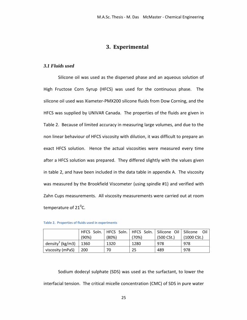
3.1 Fluids used
Silicone oil was used as the dispersed phase and an aqueous solution of
High Fructose Corn Syrup (HFCS) was used for the continuous phase. The
silicone oil used was Xiameter-PMX200 silicone fluids from Dow Corning, and the
HFCS was supplied by UNIVAR Canada. The properties of the fluids are given in
Table 2. Because of limited accuracy in measuring large volumes, and due to the
non linear behaviour of HFCS viscosity with dilution, it was difficult to prepare an
exact HFCS solution. Hence the actual viscosities were measured every time
after a HFCS solution was prepared. They differed slightly with the values given
in table 2, and have been included in the data table in appendix A. The viscosity
was measured by the Brookfield Viscometer (using spindle #1) and verified with
Zahn Cups measurements. All viscosity measurements were carried out at room
temperature of 210C.
Table 2. Properties of fluids used in experiments
HFCS Soln. (90%)
HFCS Soln. (80%)
HFCS Soln. (70%)
Silicone Oil (500 CSt.)
Silicone Oil (1000 CSt.)
density3 (kg/m3) 1360 1320 1280 978 978
viscosity (mPaS) 200 70 25 489 978
Sodium dodecyl sulphate (SDS) was used as the surfactant, to lower the
interfacial tension. The critical micelle concentration (CMC) of SDS in pure water

M.A.Sc. Thesis - M. Das McMaster - Chemical Engineering
26
at 250C is 0.0082 M (Mukherjee and Mysels, 1971), which corresponds to 2365
ppm. The experiments were carried out below this concentration-starting from
zero, low (~200 ppm), and then finally at high (~ 1000 ppm) concentration levels.
The interfacial tensions corresponding to these three levels were 40, 20 and 12
mN/m respectively. A fresh batch of HFCS solution was made between each
surfactant concentration level. The actual interfacial tension was measured for
every batch after surfactant addition to ensure that it was close to the
aforementioned values.
The interfacial tension measurements were done using the pendant drop
method with the DSA10 unit from Kruss, Germany. This device is typically used
to measure the surface tension at the liquid-air interface. However, in this case
the interfacial tension at the liquid-liquid interface was measured using a
transparent acrylic cuvette, which was filled with silicone oil. The heavier HFCS
solution was used for the drop phase, and the drop was created inside the
surrounding silicone oil. Since the cuvette was transparent, the drops were
imaged and the interfacial tension values were reported by the software based
on the analysis of the drop shape.
3.2 Experimental rig and procedure
A schematic of the experimental rig with relevant instrumentation is
shown in figure 9. The static mixer used is made of acrylic, and is surrounded by

M.A.Sc. Thesis - M. Das McMaster - Chemical Engineering
27
a mineral-oil filled light box to correct for the refractive distortion caused by the
curvature of the inner cylindrical surface. The mixer’s inner diameter is 41.18
mm and its height is 92 cm. A smaller mixer with a diameter of 15.75 mm was
also used, but because of time constraints only limited runs were obtained.
Plastic shims support the SMX inserts which fit snugly inside the column. These
SMX elements are made of titanium and have the same geometry as described in
Rao et. al (2007). They have a L/D ratio of one with a void fraction of 0.892, and
are arranged in the conventional form with each element oriented 90o with
respect to its adjacent ones.

M.A.Sc. Thesis - M. Das McMaster - Chemical Engineering
28
Figure 9. Process flow diagram with instrumentation
CW HEX
SMX Static
Mixer
Continuous
Phase Tank Dispersed
Phase Tank
Receiving
Tank
Separating
Tank
CW HEX
FTTG
FT TGPG PG
2 HP Gear
Pump
2 HP Gear
Pump
VFD VFD
I/O
card
PC with
control
software

M.A.Sc. Thesis - M. Das McMaster - Chemical Engineering
29
A 15 gallon (57 L) tank was used for the continuous phase to allow for
enough run time to capture images at flow rates of up to 10 L/min. Flowserve
rotary gear pumps (model no: 2GA) were used for both continuous and
dispersed phase sides. These were run by 2 HP AC motors, which were
controlled by a Variable Frequency Drive (VFD) that received frequency as an
input from the PC. Omega positive displacement flowmeters (FPD1002B-A)
were used to measure the volumetric flow rates. The flow rates were displayed
on the monitor, and were manually controlled by changing the input frequency
to the VFD, which ultimately changed the RPM of the motor. Recirculation lines
were used to relieve system of backpressure, to homogenize the continuous
phase after dilution and to clean the system. Heat exchangers were used only
with high viscosity fluids and at high flow rates to maintain the operating
temperature of 21o C. For most runs they were on standby as the temperature
on the thermometer did not show signs of temperature rise due to viscous
dissipation. As shown in figure 10, two entry configurations were used for the
static mixer. Continuous phase entered from the bottom centre of the mixer
when it was at high viscosity (~200 mPaS) to allow the development for fully
developed laminar flow. For the other two viscosity levels (70 and 25 mPaS),
the continuous phase entered from the side through an L-shaped tube while the
dispersed phase entered from the bottom.

M.A.Sc. Thesis - M. Das McMaster - Chemical Engineering
30
In a typical run, the continuous phase pump would first be started and
brought to a desired flow rate. The dispersed phase pump would then be
started for a set flow rate that would achieve a desired holdup . The dispersion
would then be captured by the flow visualization setup (described below). The
liquids would separate in the separating tank, with the heavier cont. phase
settling at the bottom. The continuous phase would then be drained and
transported manually to the continuous phase tank for reuse. Since the silicone
oil was bought in bulk and was the minor phase, it was seldom reused.
Especially, for the low and high surfactant concentration levels, silicone oil was
never used for more than one pass through the system. Surfactant build-up in
the silicone oil phase was therefore avoided.
Figure 10. Entry configurations for continuous and dispersed phase:a) continuous phase (70 and 25 mPaS) entering from the side and dispersed phase entering from the bottom, b) continuous phase (200 mPaS)
entering from the bottom and dispersed phase entering from the side (from Rao et al.,2007)

M.A.Sc. Thesis - M. Das McMaster - Chemical Engineering
31
3.3 Flow visualization setup and image capture
Simple backlighting technique was selected for flow visualization (shown
in figure 11). The light source was a 2000 lumens fluorescent white light bulb
with a diffuser attached to the exterior of the mixer at the light end. At the
other end, a Navitar 4X zoom lens was used with a Pixelfly QE camera, which is
capable of capturing 1280x1024 images at 12 frames per second. The camera
and the lens were placed on a manually controlled x-y-z positioner to precisely
control the field of view and the focal plane. The plane closest to the wall was
selected as the focal plane in order to minimize the possibility of out of focus
droplets at the front of the plane obscuring the ones in it. The depth of field for
the lens was determined to be 3 mm, and hence only the droplets within the first
3mm from the inner wall of the mixer were captured. The field of view was set
about four inches from the top element.
For a typical run, a sample of 200 images was taken. This was
determined to be sufficient as the number of droplets captured was enough for
the mean and standard deviation to converge. The images were taken at a
frequency such that the time period exceeded the time taken for a drop to pass
through the field of view. PCO camware software was used to trigger the image
capture and to handle the sequence of images. A 0.001 s exposure time was
used for all images.

M.A.Sc. Thesis - M. Das McMaster - Chemical Engineering
32
Figure 11. Flow Visualization Setup
3.4 Image processing and circle detection
The flowchart in figure 12 summarizes the code-in appendix B- that was
used for image processing and circle detection. It was coded in C++ , with the
OpenCV library of functions, which were used for each of the blocks in the flow
chart. The functionality and the parameters of these functions are documented
in Bradski & Kaehler (2008).

M.A.Sc. Thesis - M. Das McMaster - Chemical Engineering
33
Figure 12. Flow chart for image processing code
In the pre-processsing steps an image first goes through bilateral smoothing.
This is an edge preserving smoothing technique that is used to filter the high
frequency noise in the image. It is akin to Gaussian smoothing, except in this
case an additional parameter is used to specify the variance of the Gaussian filter
in the colour domain. It then goes through Canny edge detection routine
(described in Bradski & Kaehler (2008), pg. 151), where a gradient threshold is
used as a parameter to ignore the edges that are less prominent. These edges
would correspond to out of focus drops. The gradient threshold, therefore, is a
key parameter that determines the tolerance to out of focus drops that lie
outside the focal plane. Figures 13-15 illustrate the effect of these pre-
processing steps for a sample raw image.

M.A.Sc. Thesis - M. Das McMaster - Chemical Engineering
34
Figure 13. Sample raw image

M.A.Sc. Thesis - M. Das McMaster - Chemical Engineering
35
Figure 14. Effect of Bilateral Smoothing (edge preserving algorithm)-image is blurred except at the edges, which are still preserved
The binary image from the Canny edge detection routine is then used for the
Hough circle algorithm that uses the 21-HT version (as described in literature
review) of the algorithm. The source code for this function was slightly modified
to improve the edge gradient direction calculated from Sobel derivatives. An
important parameter in the Hough circle routine is the

M.A.Sc. Thesis - M. Das McMaster - Chemical Engineering
36
Figure 15. Binary image after Canny Edge detection
accumulator threshold, which determines the minimum number of votes that is
required in order to be included in the local maxima detection in the 2D-array.
Since the number of votes is directly proportional to the radius of the circle, the
function has to be called multiple times depending on the range of radii. This is
because for large radii range, the accumulator threshold either becomes too low
for large radii, or too high for small radii, which in turn respectively increases the
propensity of exclusion of smaller droplets or false detection of large droplets. In
this case, the function was called upon separately each for two groups of radii,
and the optimum threshold was determined on a trial an error basis. Figure 16

M.A.Sc. Thesis - M. Das McMaster - Chemical Engineering
37
shows the circles detected by the Hough circle routine for the sample raw image.
The recall and precision for this sample image are both 100%.
Figure 16. Identified Droplets
There are a few salient points on the overall performance of the
algorithm that were seen during the entire course of experimentation. They are
as follows-
-Droplets less than 40 pixels in diameter were difficult to detect. This is because
the edges for small droplets (especially at high magnification) were not
prominent. Furthermore, the accumulator threshold for the group of small radii,
was set higher for radii < 20 pixels to qualify for local maxima detection

M.A.Sc. Thesis - M. Das McMaster - Chemical Engineering
38
- The performance of the algorithm is sensitive to the quality of the images. At
high flow rates, the images taken were affected by motion blur and were not as
sharp as the sample image shown above. In these cases, the algorithm had
higher rates of false positives for radii ranging between 80-90 pixels. This
affected the distribution by introducing false peaks, and also affected D43 by
adding a small negative bias.
-The key parameters such as Canny edge threshold and the accumulator
threshold parameters had to be fine tuned for different image qualities. The
algorithm therefore cannot be considered as a plug and play function that would
work in all scenarios.
3.5 Note on measurement errors
Table 3 gives the relative errors of measured and calculated values.
Except for mass, volume and viscosity, the relative errors of other directly
measured quantities are based on observation.
Table 3. Relative errors of measured and calculated values
Quantity Relative error
volume, V ±5%
mass, m ±1%
density, ±6%
interfacial tension, ±10%
viscosity, ±1%
flow rate, Q ±5%
superficial velocity, u ±5%
capillary number, Ca ±16%
reynolds number, Re ±12%

M.A.Sc. Thesis - M. Das McMaster - Chemical Engineering
39
Error estimate on D43 measurement can only be obtained by comparing
the true value to the measured values for a large number of data points.
Because a true value can only be obtained by manually measuring the drops,
such an exercise is infeasible given the scope of the research. We can however,
identify the sources of random and systematic errors. Sources of systematic
errors are-sampling near the wall of the mixer, limited resolution of the
algorithm to detect small droplets and the algorithm`s sensitivity to image
quality-which can cause a negative bias from false positives for poor quality
images. Random errors can be attributed to drops passing behind and in front of
the focal plane, which can cause changes in light intensity and visibility of drops
in the focal plane. These errors should be small when compared to the
systematic errors. Furthermore, because the algorithm process ~200 images
(~1000 droplets) to obtain a single D43 measurement, we obtain less variability in
measurement, and hence we can say that the algorithm is not significant source
of random error.

M.A.Sc. Thesis - M. Das McMaster - Chemical Engineering
40
4. Results and Discussion
Appendix A contains the experimental data in tabulated form. The data were
mainly collected using the 41.18 mm diameter mixer. It was originally planned
to collect similar data with a smaller 15.75 mm diameter mixer, however due to
time constraints only a very limited number of runs was obtained.
It is to be noted that the effect of holdup (dispersed phase fraction) was
studied only for the case of no added surfactant, and only with continuous phase
viscosities of 25 and 70 mPa.S, and at certain flow rates. Since the effect was
minor, these points appear as clusters in the figures that follow. The rest of the
data sets were obtained at a constant holdup of 10%, while varying the
superficial velocity.
4.1 D43 trends
The D43 measure has been used instead of the Sauter mean diameter
(D32) because it places more emphasis on the larger size droplets and is therefore
better in this case as distributions from SMX mixers exhibit a significant tail.
Moreover, it is less sensitive to exclusion of smaller diameter droplets, and
hence is even more appropriate with the measurement system used, which has a
limited recall for smaller diameters.

M.A.Sc. Thesis - M. Das McMaster - Chemical Engineering
41
Figures 17, 18 and 19 show the effect of interfacial tension on D43 for
continuous phase viscosities of 25, 70 and 200 mPaS respectively. The values of
D43 have been plotted against superficial velocity to simultaneously demonstrate
the effect of interfacial tension. Low (~200 ppm) and high (~1000 ppm)
surfactant concentrations correspond to interfacial tensions of 20 and 12 mN/m
respectively, and are represented by slashes and crosses on the markers
respectively.
Figure 17. Log-log plot to show the effect of interfacial tension and viscosity ratio on D43 for c ~25 mPaS (low and high surfactant conc. correspond to 200 and 1000 ppm respectively)

M.A.Sc. Thesis - M. Das McMaster - Chemical Engineering
42
Figure 18. Log-log plot to show the effect of interfacial tension and viscosity ratio on D43 for c ~70mPaS
Figure 19. Log-log plot to show the effect of interfacial tension and viscosity ratio on D43 for c ~200 mPaS

M.A.Sc. Thesis - M. Das McMaster - Chemical Engineering
43
From the plots above, it can be seen that D43 decreases by lowering the
interfacial tension. However, the effect is less apparent at low surfactant
concentration. It is known that surfactants have diffusion kinetics (Zhang et al.,
1999), and one can speculate that this discrepancy could arise because the
interfacial concentration at a moving surface is less than the equilibrium value,
which would result in interfacial tension being larger than the measured value.
Furthermore, it can be seen in Fig. 17 &18 that except for the zero surfactant
case, the D43s are higher for the high dispersed phase viscosity (1000 cst. oil) for
a specific paring with continuous phase viscosity. These observations, combined
with the clear effect of the superficial velocity, suggest that the drop breakup is a
function of the capillary number (Ca=cucd/) and the drop viscosity, which is
conventionally taken into account with the viscosity ratio.
Figures 20, 21 and 22 show the effect of viscosity ratio on D43 at different
surfactant concentration levels. The data is the same for the plots above, except
that they have been regrouped to illustrate the effects of viscosity ratio.

M.A.Sc. Thesis - M. Das McMaster - Chemical Engineering
44
Figure 20. Log-log plot to show the effect of viscosity ratio on D43 at zero surfactant concentration (viscosity ratios arranged with respect to continuous phase viscosities- from 25 mPaS (squares) to 200 mPaS (triangle); black fill represents pairing with 1000 Cst. oil whereas no fill represents pairing with 500 Cst. oil)
0.3
3
0.01 0.10
D43
(mm
)
Superficial Velocity, ucd (m/sec)
Effect of viscosity ratio on D43 at zero surfactant concentration
p=19.6
p=36.22
p=7.0
p=12.5
p=4.3

M.A.Sc. Thesis - M. Das McMaster - Chemical Engineering
45
Figure 21. Log-log plot to show the effect of viscosity ratio on D43 at low surfactant concentration
Figure 22. Log-log plot to show the effect of viscosity ratio on D43 at high surfactant concentration

M.A.Sc. Thesis - M. Das McMaster - Chemical Engineering
46
From Figures 20-22, we see that D43 has a stronger correlation with the
continuous phase viscosity- more so than the viscosity ratio. The trend is very
consistent across all surfactant concentration levels, in that we see that D43
decreases with increasing continuous phase viscosity. However, for a specific
continuous phase viscosity, D43s are higher when paired with the 1000 cst. oil
than paired with the 500 cst. oil. Again the results indicate that hydrodynamic
and surface forces are at play here.
Figure 23 shows the effect of the number of elements on D43. The
numbers were varied between six and ten.
Figure 23. Effect of number of elements on D43

M.A.Sc. Thesis - M. Das McMaster - Chemical Engineering
47
The values of D43 are consistently higher with six elements. Since the system is
dilute (), this observation cannot be attributed to drop coalescence. As
mentioned in Fradette et al. (2007), in addition to the nature of the flow field,
the residence time inside the mixer elements is very important. If the mean
residence time is less than the time required to break the drop then size
reduction may not be achieved. This phenomenon can also be modelled by the
equation given by Middleman (1974).
4.2 Dmax trends
Figures 24, 25 and 26 show the effect of Interfacial tension and superficial
velocity on Dmax, which is the maximum droplet size found in the distribution.
Figure 24. Effect of interfacial tension and viscosity ratio on Dmax for c ~25 mPaS

M.A.Sc. Thesis - M. Das McMaster - Chemical Engineering
48
Figure 25. Effect of interfacial tension and viscosity ratio on Dmax for c ~70 mPaS
Figure 26. Effect of interfacial tension and viscosity ratio on Dmax for c ~200 mPaS

M.A.Sc. Thesis - M. Das McMaster - Chemical Engineering
49
It can be seen that for low continuous phase viscosity and zero surfactant
concentration, Dmax is in the vicinity of 5 mm. Very limited data was also
obtained with a mixer diameter of 15.75 mm. Dmax values for these three runs
were approximately 1.5 mm. These two values are very close to the measured
gaps (5 mm and 1.5 mm respectively) between the cross bars for 41.18 and
15.75 mm diameter mixer elements. This observation suggests that there is
effectively a slicing action of the crossbars to determine the initial drop size. If
these drops are not broken any further, due to inadequate hydrodynamic forces
or residence times further up the mixer, then they appear as oversize drops in
the distribution. This “slicing” action is also shown in the section Qualitative
Images below.
4.3 Droplet size distribution trends
Table 4 compares the droplet size distributions at low and high superficial
velocities and at different viscosity ratios-all obtained at zero surfactant
concentration. The low values range from 1.5-2 L/min, whereas the high values
range from 6-8 L/min (Please see Appendix A for specific values for the given run
numbers).

M.A.Sc. Thesis - M. Das McMaster - Chemical Engineering
50
Table 4. Droplet size distribution trends at zero surfactant concentration
Superficial Velocity
Low High
p=36.2
(c=27 mPaS,
d=978 mPaS)
p=19.6
(c=27 mPaS,
d=489 mPaS)
0%
2%
4%
6%
8%
10%
12%
14%
0 1 2 3 4 5 6
Fre
qu
en
cy
Diameter (mm)
DSD Run 41
0%
2%
4%
6%
8%
10%
12%
14%
0 1 2 3 4 5 6
Fre
qu
en
cy
Diameter (mm)
DSD Run 23

M.A.Sc. Thesis - M. Das McMaster - Chemical Engineering
51
Superficial Velocity
Low High
p=12.5
(c=78 mPaS,
d=978 mPaS)
p=4.3
(c=230 mPaS,
d=489 mPaS)
0%
2%
4%
6%
8%
10%
12%
14%
16%
0 1 2 3 4 5 6
Fre
qu
en
cy
Diameter (mm)
DSD Run 36
0%
2%
4%
6%
8%
10%
12%
14%
0 1 2 3 4 5 6
Fre
qu
en
cy
Diameter (mm)
DSD Run 27
0%
2%
4%
6%
8%
10%
12%
14%
16%
0 1 2 3 4 5 6
Fre
qu
en
cy
Diameter (mm)
DSD Run 29

M.A.Sc. Thesis - M. Das McMaster - Chemical Engineering
52
The general trend for these distributions is that the frequency of occurrence is
more or less the same (i.e. we see a plateau) in a specific diameter range. This is
followed by a tail that becomes smaller and narrower with increasing continuous
phase viscosity and superficial velocity. As explained in the previous section, it
can be inferred that for a given residence time inside the mixer, size reduction is
achieved as the hydrodynamic forces increase in relation to the interfacial forces.
For some runs-as in Run 38 for example-the distributions show a sharp cutoff in
the droplet size. This however, is a result of the Hough circle detection
algorithm’s propensity to detect false positives within a range (which in this case
is 2 mm) when the image quality is poor.
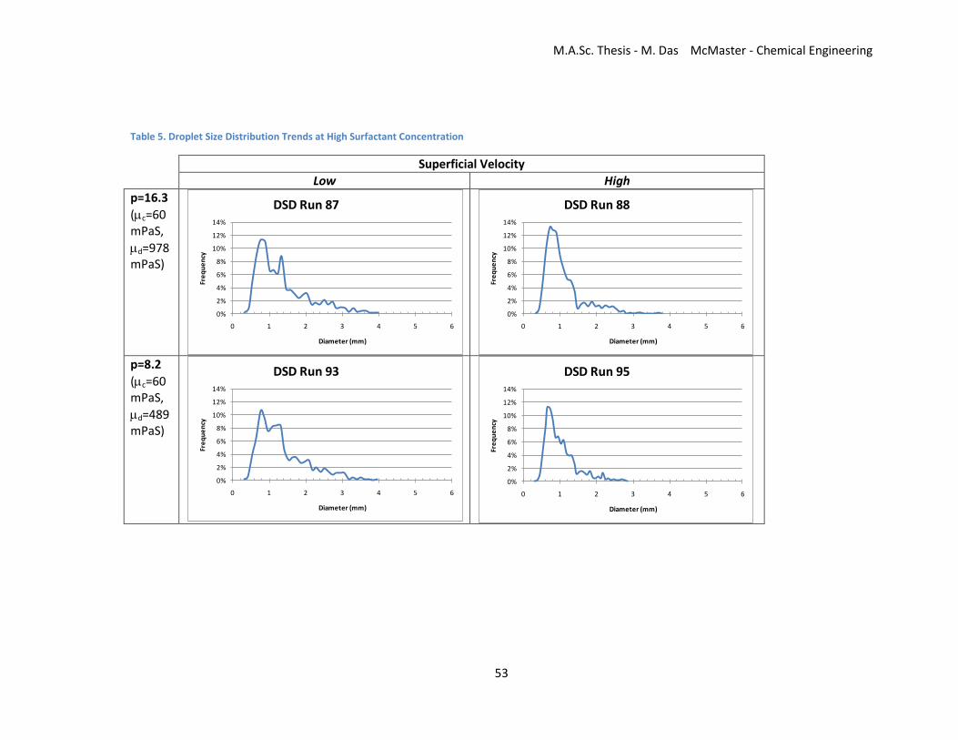
Table 5 compares the same, but at high surfactant concentration (~1000
ppm).
M.A.Sc. Thesis - M. Das McMaster - Chemical Engineering
53
Table 5. Droplet Size Distribution Trends at High Surfactant Concentration
Superficial Velocity
Low High
p=16.3
(c=60 mPaS,
d=978 mPaS)
p=8.2
(c=60 mPaS,
d=489 mPaS)
0%
2%
4%
6%
8%
10%
12%
14%
0 1 2 3 4 5 6
Fre
qu
en
cy
Diameter (mm)
DSD Run 87
0%
2%
4%
6%
8%
10%
12%
14%
0 1 2 3 4 5 6
Fre
qu
en
cy
Diameter (mm)
DSD Run 88
0%
2%
4%
6%
8%
10%
12%
14%
0 1 2 3 4 5 6
Fre
qu
en
cy
Diameter (mm)
DSD Run 93
0%
2%
4%
6%
8%
10%
12%
14%
0 1 2 3 4 5 6Fr
eq
ue
ncy
Diameter (mm)
DSD Run 95
M.A.Sc. Thesis - M. Das McMaster - Chemical Engineering
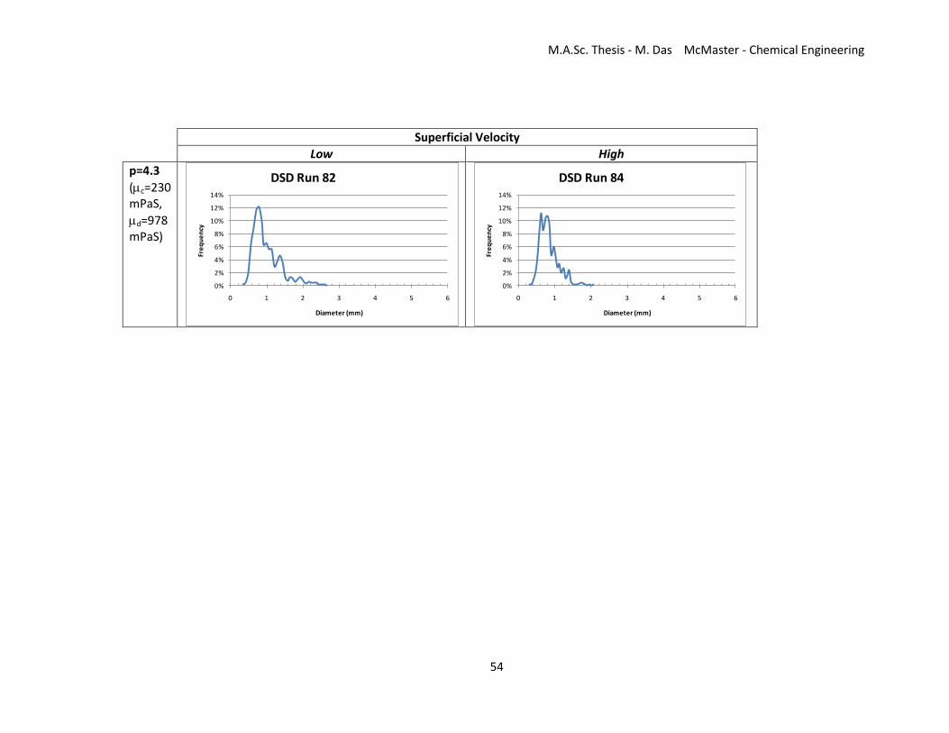
54
Superficial Velocity
Low High
p=4.3
(c=230 mPaS,
d=978 mPaS)
0%
2%
4%
6%
8%
10%
12%
14%
0 1 2 3 4 5 6
Fre
qu
en
cy
Diameter (mm)
DSD Run 82
0%
2%
4%
6%
8%
10%
12%
14%
0 1 2 3 4 5 6
Fre
qu
en
cy
Diameter (mm)
DSD Run 84

M.A.Sc. Thesis - M. Das McMaster - Chemical Engineering
55
We see that at high surfactant concentration the distributions tend to resemble
a log-normal distribution. It tends towards becoming a Gaussian (as in the case
with run 84), with increasing superficial velocity and continuous phase viscosity.
This could be because of a change in breakup mechanism as a result of the
addition of surfactant. A possible candidate for a dominant mechanism could be
tip streaming, since the breakup of a large number of daughter droplets from the
tip of a large mother droplet gives rise to a log-normal distribution. This
conjecture is further supported by Janssen (1997), wherein tip streaming has
been described as being more favourable with moderate surfactant
concentration.
4.4 Qualitative Images
Images were also taken inside the third element (from the bottom) of the
mixer. The purpose of this was to get a qualitative view of the drop breakup
mechanism inside the mixer. Figure 27 shows the breakup of a stream as it
passes through the gap between the crossbars. In figure 28, an image sequence
is shown that demonstrates the drop breakup from collision with cross -points as
described in Liu (2005) and shown in Figure 29.

M.A.Sc. Thesis - M. Das McMaster - Chemical Engineering
56
Figure 27. A frame from an image sequence showing the breakup of a dispersed phase stream into drops as it is passes through the gap between the cross bars
Figure 28. Image sequence showing drop breakup from impact with cross-points of the packing

M.A.Sc. Thesis - M. Das McMaster - Chemical Engineering
57
Figure 29. Image sequence showing a single drop breakup at cross-point (Liu, 2005)
From the images above, we can conclude that there are multiple breakup
mechanisms occurring inside the mixer. Furthermore, as seen in fig. 27, the
slicing mechanism is seen wherein the dispersed phase stream is stretched as it
passes through the gap between the cross bars, and ultimately breaks due the
extensional and compression regions in the surrounding three dimensional flow
field.
4.5 Proposed Model
An observation-based model has been proposed by Dr. Baird. A drop can
be said to breakup in a 2-stage process-
-The first stage is the initial formation of primary drops (with diameter D0), which
forms with the interaction with the packing. The diameter D0 is of the same
order of magnitude as the gap between the adjacent plates in the packing.

M.A.Sc. Thesis - M. Das McMaster - Chemical Engineering
58
-Secondary drops with diameter, D<D0 are formed by a mechanism of viscous
shear as described in Janssen et al. (1997) and Christini et al. (2003). The final
distribution contains a few relatively large drops and a much larger number of
smaller ones.
We equate the work done by viscous shear with the increase in surface
energy owing to the size reduction from D0->Df. Consider a large number of N0
drops of diameter D0 undergoing breakup to diameter Df (<D0). Then by
continunity the number of drops N is given by
(28)
and the relative increase in surface area is given by
(29)
from eq (28) and (29), the above simplifies to
(30)
Therefore the increase in suface energy per single drop is given by
(31)

M.A.Sc. Thesis - M. Das McMaster - Chemical Engineering
59
where is the interfacial tension.
Work done on the initial drop by viscous shear is proportional to
(32)
By assuming a shear rate of
, the proportionality above can be written as
(33)
Since the increase in surface energy is proportional to work done for
breakup we get,
(34)
which simplifies to
(35)
where Ca is the capillary number. Therefore D0, Df and Ca can be related by the
equation
(36)

M.A.Sc. Thesis - M. Das McMaster - Chemical Engineering
60
where k is an unknown proportionality constant. However, we now have a basis
to plot the data. If we assume Df≈D43, then we can plot 1/D43 Vs Ca, where the
intercept would be 1/D0.
In Figure 29, 1/D43 has been plotted against where p is the
viscosity ratio . Since the dispersed phase viscosity has not been considered in
the above energy analysis, the capillary number has been multiplied by the
viscosity ratio to the nth power. The value of the exponent n that gives the best
linear fit has to be determined. Furthermore, since we suspect that the actual
interfacial tension is higher than the measured interfacial tension because of
diffusion kinetics, a reduction factor is used. It is the fraction of reduction of the
Figure 30. Model assessment by correlating D43 with capillary number
R² = 0.8784
0.00
0.50
1.00
1.50
2.00
2.50
0.00 0.05 0.10 0.15 0.20 0.25 0.30 0.35 0.40 0.45
D4
3-1
(mm
-1)
Ca*pn
Model assessment: correlation with capillary number and viscosity ratio
data with 41.18 mm dia.
data with 15.75 mm dia.

M.A.Sc. Thesis - M. Das McMaster - Chemical Engineering
61
interfacial tension from zero surfactant to low or high surfactant concentration.
From Excel solver, the best values of n and the reduction factor were determined
to be -0.66 and 0.98 respectively. This gives a reasonably good fit with a R^2
value of 0.88. The trend line (for 41.18 mm dia.) intercepts the vertical axis at
approximately 0.25, which corresponds to D43 ≈4 mm. Although, the data set for
the 15.75 mm dia. is not large enough to substantiate any claim, however, it
does seem to intercept the y-axis at ~0.6 mm, which corresponds to a D43≈ 1.7
mm. Since both 4 mm and 1.7 mm are values that we might expect for D0, we
can say that the model is a good starting point. It might be improved by
considering the effect of internal resistance of the drop phase viscosity in the
energy analysis.

M.A.Sc. Thesis - M. Das McMaster - Chemical Engineering
62
5. Conclusion
5.1 Summary
In this research, liquid-liquid dispersion of viscous fluids was studied in an
SMX static mixer in the laminar regime. Backlighting technique was used for
flow visualization, and Hough transform for circle detection was used in OpenCV
to automatically detect and measure drops for obtaining the size distribution.
Silicone oil and an aqueous solution of high fructose corn syrup were used for
dispersed and continuous phases respectively, and sodium dodecyl sulfate was
used as the surfactant to lower the interfacial tension. Experiments were
conducted at varying viscosity ratios and flow rates-each at zero, low and high
surfactant concentrations. The effect of holdup was explored only at specific
viscosity ratios and at certain flow rates, and it was found to have a minimal
effect on D43. Further observations made were the following-
Superficial velocity and continuous phase viscosity seemed to have a
dominant effect on D43. The effect of dispersed phase viscosity was
significant only at low and high surfactant concentrations.
There was a measurable decrease in D43 at low surfactant concentration,
and a significant decrease at high surfactant concentration. This
confirmed that there is an effect of interfacial tension.

M.A.Sc. Thesis - M. Das McMaster - Chemical Engineering
63
Droplet size distributions typically were found to have a long and wide
tail, which became narrower and shorter with higher superficial
velocities, higher continuous phase viscosities, and lower interfacial
tension. For the lowest interfacial tension (high surfactant
concentration), the size distribution was log-normal.
The gap between cross bars (or adjacent plates) in the packing seemed to
determine a primary diameter, which appeared as Dmax in the absence
of major dispersion further up in the packing. This observation is
consistent with Catalfamo et al. (2003), whereby size reduction during
scale up was maintained by keeping the surface area to void volume ratio
of the elements constant. This was done by addition of more cross bars
for larger diameter elements.
Finally, a simple model relating D43 to capillary number was proposed (by Dr.
Baird). The model is based on equating the work done in breaking a primary
drop by hydrodynamic forces to the increase in surface energy of the drops. It
was found to fit the data reasonably well, and it could prove to be a promising
starting point for more detailed analysis that would take into account the effect
of dispersed phase viscosity and holdup. The model was qualitatively supported
by limited data from a smaller SMX cartridge (15.75 mm diameter)

M.A.Sc. Thesis - M. Das McMaster - Chemical Engineering
64
5.2 Recommendations for future work
Based on the experience from conducting the experiments, the following
suggestions are made to improve the experimental apparatus and the flow
visualization/image acquisition system-
Use of high speed cameras and large aperture zoom lens to get high
quality images (without motion blur) with crisp images at high flow rates.
This will aid in increasing the recall and precision of the algorithm in these
cases
Inclusion of a recycling line (by means of a 3-way valve) from the
separating tank for the continuous phase to avoid manual reloading of
the continuous phase tank
Recommendations for further studies are as follows-
Identification of droplet breakup mechanisms further up the packing-by
taking images of its interiors- for different viscosity ratios and surfactant
concentrations
Validations of the influence of the gaps between adjacent plates in the
packing, by possibly altering the number of cross bars in its geometry, or
by carrying out detailed experiments with different sizes of SMX
cartridge.

M.A.Sc. Thesis - M. Das McMaster - Chemical Engineering
65
References
Bentley, B.J., & Leal, L.G. (1986). An experimental investigation of drop
deformation and breakup in steady two-dimensional linear flow. Journal
of Fluid Mechanics, 167, 241–283.
Berkman, P.D., & Calabrese, R.V. (1988). Dispersion of viscous liquids by
turbulent flow in a static mixer. A.I.Ch.E. Journal, 34, 602–609.
Brás, L.M.R., Gomes, E.F., Ribeiro, M.M.M., & Guimarães, M.M.L.(2009). Drop Distribution Determination in a Liquid-Liquid Dispersion by
Image Processing. International Journal of Chemical Engineering,
746439 -746439.
Bradski, G., & Kaehler, A. (2008). Learning OpenCV: Computer Vision with the
OpenCV. Sebastopol, CA: O’Reilly Media Inc.
Catalfamo, V., Blum, G.L., & Jaffer, S.A. (2003). US Patent No. 6,550,960.
Washington, D.C.: U.S. Patent and Trademark Office
Christini, V., Guido, S., Alfani, A., Blawzdziewicz, J., & Lowenberg, M. (2003).
Drop breakup and fragment size distribution in shear flow. Journal of
Rheology, 47, 1283-1298.
Das, P. K., Legrand, J., Morançais, P., & Carnelle, G. (2005). Drop breakage
model in static mixers at low and intermediate Reynolds number.
Chemical Engineering Science, 60, 231-238.
De Bruijn, R.A. (1993). Tipstreaming of drops in simple shear flows. Chemical
Engineering Science, 48, 277-284.
Fradette, L., Tanguy, P., Li, H.Z., & Choplin, L. (2007). Liquid/Liquid Viscous
Dispersions with a SMX Static Mixer. Chemical Engineering Research
and Design, 85, 395-405.
Grace, H.P. (1982). Dispersion phenomena in high viscosity immiscible fluid
systems and application of static mixers as dispersion devices in such
systems. Chemical Engineering Communications, 14, 225–277.
Janssen, J.J.M., Boon, A., & Agterof, W.G.W. (1997). Influence of dynamic
interfacial properties on droplet breakup in plane hyperbolic flow.
A.I.Ch.E. Journal, 43, 1436–1447.

M.A.Sc. Thesis - M. Das McMaster - Chemical Engineering
66
Karbstein, H., & Schubert, H. (1995). Developments in the continuous
mechanical production of oil-in-water macro-emulsions. Chem.Eng. Proc,
34: 205–211
Kim, I.G., & Lee, S.Y. (1990). Simple technique for sizing and counting spray
drops using digital image processing. Experimental Thermal and Fluid
Science, 3, 214-221.
Legrand, J., Morançais, P., & Carnelle, G. (2001). Liquid–liquid dispersion in a
SMX-Sulzer static mixer. Chemical Engineering Research & Design, 79,
949–956.
Liu, S. (2005). Ph.D. Thesis: Laminar mixing in an SMX static mixer. Hamilton,
ON: McMaster University.
Liu, S.J., Hrymak, A.N., & Wood, P.E. (2005). Drop breakup in an SMX mixer
in laminar flow. Canadian Journal of Chemical Engineering, 83, 793–
807.
Middleman, S. (1974). Drop size distributions produced by turbulent pipe flow of
immiscible fluids through a static mixer. I&EC Process Design and
Developments, 13(1), 78–83.
Paul, E.L., Atiemo-Obeng, V., & Kresta, S.M. (2004). Handbook of industrial
mixing: Science and Practice. Hoboken, NJ: John Wiley & Sons Inc.
Mukherjee, P. & Mysels K.J. (1971). Critical micelle concentration of aqueous
surfactant systems. NSRDS-NBS 36. Washington, D.C.: Office of
Standards Reference Data
Rama Rao, N. V., Baird, M. H. I., Hrymak, A. N., & Wood, P. E. (2007).
Dispersion of high-viscosity liquid-liquid systems by flow through SMX
static mixer elements. Chemical Engineering Science, 62, 6885-6896.
Rauline, D., Tanguy, P.A., Le Blevec, J.-M., & Bousquet, J. (1998). Numerical
investigation of performance of several static mixers. Candian Journal of
Chemical Engineering, 76, 527–535.
Streiff, F. (1977). In-line dispersion and mass transfer using static mixing
equipment. Sulzer Technol, 108.
Streiff, F., Mathys, P., & Fischer, T.U. (1997). New fundamentals for liquid–
liquid dispersion using static mixers. Recents Progrés en Genie des
Procedés, 11(51), 307–314.

M.A.Sc. Thesis - M. Das McMaster - Chemical Engineering
67
Stone, H.A., & Leal, L.G. (1989). Relaxation and breakup of an initially extended
drop in an otherwise quiescent fluid. Journal of Fluid Mechanics, 198,
399-427.
Thakur, R. K., Vial, C., Nigam, K. D. P., & Nauman, E. B., Djelveh, G. (2003).
Static mixers in the process industries: A review. Chemical Engineering
Research and Design, 81, 787-826.
Theron, F., Le Sauze, N., & Ricard, A. (2010). Turbulent Liquid-Liquid
Dispersion in Sulzer SMX Mixer. Ind. Eng. Chem. Res., 49, 623–632.
Yuen, H.K., Princen, J., Illingworth, J., & Kittler, J. (1990). Comparitive study
of Hough Transform methods for circle finding. Image and vision
computing, 8, 71 -7.
Zhang, J., & Pelton, R. (1999). Application of polymer adsorption models to
dynamic surface tension. Langmuir, 15, 5662-5669.

Appendix A Tabulated Experimental Data

A1
Note: The tabulated data below was used in the Result and Discussion section
Capillary number defined as
Run #
Cell
Diameter
(m)
No.
Elements
c
(Pa.S)
d
(Pa.S) p
(N/m)
qc
(m3/sec)
qd
(m3/sec)
ucd
(m/sec) h RecdCa
D43
(mm)
Dmax
(mm)
1 4.12E-02 10 7.00E-02 4.89E-01 7.0 4.00E-02 1.02E-05 5.00E-06 1.14E-02 0.33 8.66 1.99E-02 3.39 5.44
2 4.12E-02 10 7.00E-02 4.89E-01 7.0 4.00E-02 3.55E-05 6.50E-06 3.15E-02 0.15 23.98 5.52E-02 2.95 5.23
3 4.12E-02 10 7.00E-02 4.89E-01 7.0 4.00E-02 6.83E-05 1.77E-05 6.46E-02 0.21 49.11 1.13E-01 2.36 1.89
4 4.12E-02 10 7.00E-02 4.89E-01 7.0 4.00E-02 1.20E-04 1.30E-05 9.97E-02 0.10 75.85 1.75E-01 1.89 5.58
5 4.12E-02 10 7.00E-02 4.89E-01 7.0 4.00E-02 1.46E-04 3.07E-05 1.33E-01 0.17 100.98 2.32E-01 1.43 4.86
6 1.58E-02 10 7.00E-02 4.89E-01 7.0 4.00E-02 1.03E-05 1.67E-06 6.16E-02 0.14 17.92 1.08E-01 0.99 4.86
7 1.58E-02 10 7.00E-02 4.89E-01 7.0 4.00E-02 1.72E-05 2.33E-06 1.00E-01 0.12 29.11 1.75E-01 0.77 4.86
8 1.58E-02 10 7.00E-02 4.89E-01 7.0 4.00E-02 1.58E-05 2.33E-06 9.32E-02 0.13 27.12 1.63E-01 0.72 4.86
9 4.12E-02 6 7.80E-02 4.89E-01 6.3 4.00E-02 1.13E-05 4.50E-06 1.19E-02 0.28 8.11 2.32E-02 3.85 4.86
10 4.12E-02 6 7.80E-02 4.89E-01 6.3 4.00E-02 3.65E-05 6.50E-06 3.23E-02 0.15 22.04 6.30E-02 3.47 5.44
11 4.12E-02 6 7.80E-02 4.89E-01 6.3 4.00E-02 6.92E-05 1.77E-05 6.52E-02 0.20 44.50 1.27E-01 2.94 5.26
12 4.12E-02 6 7.80E-02 4.89E-01 6.3 4.00E-02 1.22E-04 1.30E-05 1.01E-01 0.10 69.01 1.97E-01 2.43 4.46
13 4.12E-02 6 7.80E-02 4.89E-01 6.3 4.00E-02 1.75E-04 7.83E-06 1.38E-01 0.04 93.87 2.68E-01 2.15 3.82
14 4.12E-02 6 2.50E-02 4.89E-01 19.6 4.00E-02 3.87E-05 1.73E-05 4.20E-02 0.31 89.40 2.62E-02 3.52 5.53
15 4.12E-02 6 2.50E-02 4.89E-01 19.6 4.00E-02 6.32E-05 1.33E-05 5.74E-02 0.17 122.31 3.59E-02 3.50 5.49
16 4.12E-02 6 2.50E-02 4.89E-01 19.6 4.00E-02 8.67E-05 2.33E-05 8.25E-02 0.21 175.74 5.16E-02 3.13 5.25
17 4.12E-02 6 2.50E-02 4.89E-01 19.6 4.00E-02 1.13E-04 1.43E-05 9.59E-02 0.11 204.12 5.99E-02 3.12 4.77
18 4.12E-02 6 2.50E-02 4.89E-01 19.6 4.00E-02 1.42E-04 7.42E-06 1.12E-01 0.05 239.43 7.03E-02 2.89 4.79
19 4.12E-02 10 2.50E-02 4.89E-01 19.6 4.00E-02 3.65E-05 1.77E-05 4.07E-02 0.33 86.61 2.54E-02 3.14 5.23
20 4.12E-02 10 2.50E-02 4.89E-01 19.6 4.00E-02 6.60E-05 1.30E-05 5.93E-02 0.16 126.31 3.71E-02 3.14 5.95
21 4.12E-02 10 2.50E-02 4.89E-01 19.6 4.00E-02 7.30E-05 2.30E-05 7.21E-02 0.24 153.49 4.50E-02 2.89 4.65

A2
Run #
Cell
Diameter
(m)
No.
Elements
c
(Pa.S)
d
(Pa.S) p
(N/m)
qc
(m3/sec)
qd
(m3/sec)
ucd
(m/sec) h Recd Ca
D43
(mm)
Dmax
(mm)
22 4.12E-02 10 2.50E-02 4.89E-01 19.6 4.00E-02 1.43E-04 7.67E-06 1.13E-01 0.05 241.43 7.09E-02 2.62 4.11
23 4.12E-02 10 2.50E-02 4.89E-01 19.6 4.00E-02 1.10E-04 1.43E-05 9.34E-02 0.12 198.79 5.83E-02 2.39 4.47
24 4.12E-02 10 2.45E-01 4.89E-01 2.0 4.00E-02 4.74E-05 1.16E-05 4.43E-02 0.20 9.63 2.71E-01 0.89 1.82
25 4.12E-02 10 2.45E-01 4.89E-01 2.0 4.00E-02 4.96E-05 8.25E-06 4.34E-02 0.14 9.44 2.66E-01 0.90 1.75
26 4.12E-02 10 2.45E-01 4.89E-01 2.0 4.00E-02 5.58E-05 3.50E-06 4.45E-02 0.06 9.68 2.73E-01 1.02 1.66
27 4.12E-02 10 2.30E-01 9.78E-01 4.3 4.00E-02 4.57E-05 4.50E-06 3.77E-02 0.09 8.72 2.17E-01 2.07 3.67
28 4.12E-02 10 2.30E-01 9.78E-01 4.3 4.00E-02 6.67E-05 7.83E-06 5.59E-02 0.11 12.95 3.22E-01 1.46 2.80
29 4.12E-02 10 2.30E-01 9.78E-01 4.3 4.00E-02 9.33E-05 1.03E-05 7.78E-02 0.10 18.02 4.48E-01 0.94 1.89
31 4.12E-02 10 2.30E-01 9.78E-01 4.3 4.00E-02 1.18E-04 1.16E-05 9.70E-02 0.09 22.46 5.58E-01 0.69 1.31
32 4.12E-02 10 7.80E-02 9.78E-01 12.5 4.00E-02 8.23E-05 3.83E-06 6.47E-02 0.04 44.16 1.26E-01 2.52 4.23
33 4.12E-02 10 7.80E-02 9.78E-01 12.5 4.00E-02 7.50E-05 8.33E-06 6.26E-02 0.10 42.71 1.22E-01 2.41 4.03
34 4.12E-02 10 7.80E-02 9.78E-01 12.5 4.00E-02 7.30E-05 1.30E-05 6.46E-02 0.15 44.07 1.26E-01 2.25 4.30
35 4.12E-02 10 7.80E-02 9.78E-01 12.5 4.00E-02 6.92E-05 1.63E-05 6.42E-02 0.19 43.82 1.25E-01 2.25 3.53
36 4.12E-02 10 7.80E-02 9.78E-01 12.5 4.00E-02 1.04E-04 1.10E-05 8.61E-02 0.10 58.76 1.68E-01 2.10 3.94
37 4.12E-02 10 7.80E-02 9.78E-01 12.5 4.00E-02 1.36E-04 1.43E-05 1.13E-01 0.10 76.91 2.20E-01 1.73 3.44
38 4.12E-02 10 7.80E-02 9.78E-01 12.5 4.00E-02 3.67E-05 3.83E-06 3.04E-02 0.09 20.75 5.93E-02 3.20 5.55
39 4.12E-02 10 2.70E-02 9.78E-01 36.2 4.00E-02 5.33E-05 6.50E-06 4.49E-02 0.11 88.58 3.03E-02 3.63 5.58
40 4.12E-02 10 2.70E-02 9.78E-01 36.2 4.00E-02 7.77E-05 8.83E-06 6.49E-02 0.10 128.06 4.38E-02 3.30 5.38
41 4.12E-02 10 2.70E-02 9.78E-01 36.2 4.00E-02 1.02E-04 1.20E-05 8.53E-02 0.11 168.28 5.76E-02 3.06 4.61
42 4.12E-02 10 2.70E-02 9.78E-01 36.2 4.00E-02 1.30E-04 1.48E-05 1.09E-01 0.10 214.42 7.34E-02 2.65 4.20
43 4.12E-02 10 2.70E-02 9.78E-01 36.2 4.00E-02 6.67E-05 1.77E-05 6.33E-02 0.21 124.85 4.27E-02 3.20 5.58
44 4.12E-02 10 2.70E-02 9.78E-01 36.2 2.30E-02 5.67E-05 6.50E-06 4.74E-02 0.10 93.51 5.57E-02 3.39 4.84
45 4.12E-02 10 2.70E-02 9.78E-01 36.2 2.30E-02 9.58E-05 8.83E-06 7.86E-02 0.08 154.95 9.23E-02 2.90 4.28

A3
Run #
Cell
Diameter
(m)
No.
Elements
c
(Pa.S)
d
(Pa.S) p
(N/m)
qc
(m3/sec)
qd
(m3/sec)
ucd
(m/sec) h Recd Ca
D43
(mm)
Dmax
(mm)
46 4.12E-02 10 2.70E-02 9.78E-01 36.2 2.30E-02 1.15E-04 1.15E-05 9.50E-02 0.09 187.28 1.11E-01 2.60 4.87
47 4.12E-02 10 2.70E-02 9.78E-01 36.2 2.30E-02 1.41E-04 1.50E-05 1.17E-01 0.10 230.70 1.37E-01 2.30 4.41
48 4.12E-02 10 2.70E-02 9.78E-01 36.2 2.30E-02 6.13E-05 6.50E-06 5.09E-02 0.10 100.42 5.98E-02 3.19 4.72
49 4.12E-02 10 2.70E-02 9.78E-01 36.2 2.30E-02 2.50E-05 6.50E-06 2.37E-02 0.21 46.63 2.78E-02 3.37 4.86
53 4.12E-02 10 2.70E-02 4.89E-01 18.1 2.30E-02 2.50E-05 5.00E-06 2.25E-02 0.17 44.41 2.64E-02 3.41 5.09
54 4.12E-02 10 2.70E-02 4.89E-01 18.1 2.30E-02 1.13E-04 1.30E-05 9.49E-02 0.10 187.03 1.11E-01 2.18 4.13
55 4.12E-02 10 2.70E-02 4.89E-01 18.1 2.30E-02 8.50E-05 8.83E-06 7.05E-02 0.09 138.91 8.27E-02 2.60 4.41
56 4.12E-02 10 2.70E-02 4.89E-01 18.1 2.30E-02 1.48E-04 1.63E-05 1.24E-01 0.10 243.78 1.45E-01 1.88 3.57
57 4.12E-02 10 2.70E-02 4.89E-01 18.1 2.30E-02 5.83E-05 6.50E-06 4.87E-02 0.10 95.98 5.71E-02 2.92 5.09
58 4.12E-02 10 2.70E-02 4.89E-01 18.1 2.30E-02 9.00E-05 4.17E-06 7.07E-02 0.04 139.41 8.30E-02 2.38 4.31
59 4.12E-02 10 2.70E-02 4.89E-01 18.1 2.30E-02 7.67E-05 1.50E-05 6.88E-02 0.16 135.71 8.08E-02 2.70 4.72
60 4.12E-02 10 7.40E-02 4.89E-01 6.6 2.30E-02 6.68E-05 6.50E-06 5.51E-02 0.09 39.61 1.77E-01 2.12 3.88
61 4.12E-02 10 7.40E-02 4.89E-01 6.6 2.30E-02 3.05E-05 3.33E-06 2.54E-02 0.10 18.28 8.17E-02 2.57 4.53
62 4.12E-02 10 7.40E-02 4.89E-01 6.6 2.30E-02 1.02E-04 1.00E-05 8.38E-02 0.09 60.32 2.70E-01 1.54 3.18
64 4.12E-02 10 7.40E-02 4.89E-01 6.6 2.30E-02 1.43E-04 1.53E-05 1.19E-01 0.10 85.71 3.83E-01 1.12 2.33
65 4.12E-02 6 7.40E-02 4.89E-01 6.6 2.30E-02 1.02E-04 1.12E-05 8.47E-02 0.10 60.95 2.73E-01 1.89 3.29
66 4.12E-02 6 7.40E-02 4.89E-01 6.6 2.30E-02 1.37E-04 1.50E-05 1.14E-01 0.10 81.92 3.66E-01 1.46 3.01
67 4.12E-02 6 7.40E-02 4.89E-01 6.6 2.30E-02 6.00E-05 7.67E-06 5.08E-02 0.11 36.55 1.63E-01 2.85 4.97
68 4.12E-02 6 7.40E-02 4.89E-01 6.6 2.30E-02 2.83E-05 3.33E-06 2.38E-02 0.11 17.11 7.65E-02 3.41 5.21
69 4.12E-02 6 7.40E-02 4.89E-01 6.6 2.30E-02 7.75E-05 8.33E-06 6.44E-02 0.10 46.36 2.07E-01 2.65 4.66
71 4.12E-02 10 7.40E-02 9.78E-01 13.2 2.30E-02 3.28E-05 3.58E-06 2.73E-02 0.10 19.67 8.80E-02 3.21 5.37
72 4.12E-02 10 7.40E-02 9.78E-01 13.2 2.30E-02 6.27E-05 7.42E-06 5.26E-02 0.11 37.86 1.69E-01 2.67 4.78
73 4.12E-02 10 7.40E-02 9.78E-01 13.2 2.30E-02 8.03E-05 8.67E-06 6.68E-02 0.10 48.07 2.15E-01 2.52 4.32

A4
Run #
Cell
Diameter
(m)
No.
Elements
c
(Pa.S)
d
(Pa.S) p
(N/m)
qc
(m3/sec)
qd
(m3/sec)
ucd
(m/sec) h RecdCa
D43
(mm)
Dmax
(mm)
74 4.12E-02 10 7.40E-02 9.78E-01 13.2 2.30E-02 1.49E-04 1.43E-05 1.23E-01 0.09 88.32 3.95E-01 2.18 4.08
75 4.12E-02 10 7.40E-02 9.78E-01 13.2 2.30E-02 1.03E-04 1.30E-05 8.68E-02 0.11 62.48 2.79E-01 2.27 4.11
76 4.12E-02 10 7.40E-02 9.78E-01 13.2 2.30E-02 1.34E-04 1.38E-05 1.11E-01 0.09 79.58 3.56E-01 2.27 4.06
77 4.12E-02 10 2.30E-01 9.78E-01 4.3 2.30E-02 4.57E-05 4.50E-06 3.77E-02 0.09 8.72 3.77E-01 1.78 3.30
78 4.12E-02 10 2.30E-01 9.78E-01 4.3 2.30E-02 7.30E-05 7.67E-06 6.06E-02 0.10 14.02 6.06E-01 1.16 2.29
79 4.12E-02 10 2.30E-01 9.78E-01 4.3 2.30E-02 9.69E-05 1.00E-05 8.03E-02 0.09 18.58 8.03E-01 0.82 1.86
80 4.12E-02 10 2.30E-01 9.78E-01 4.3 2.30E-02 1.14E-04 1.30E-05 9.52E-02 0.10 22.04 9.52E-01 0.61 1.44
81 4.12E-02 10 2.30E-01 9.78E-01 4.3 2.30E-02 2.83E-05 3.33E-06 2.38E-02 0.11 5.50 2.38E-01 1.97 3.55
82 4.12E-02 10 2.30E-01 9.78E-01 4.3 1.30E-02 2.89E-05 3.58E-06 2.44E-02 0.11 5.65 4.32E-01 1.55 3.17
83 4.12E-02 10 2.30E-01 9.78E-01 4.3 1.30E-02 4.83E-05 5.00E-06 4.00E-02 0.09 9.27 7.08E-01 1.27 2.42
84 4.12E-02 10 2.30E-01 9.78E-01 4.3 1.30E-02 7.00E-05 7.17E-06 5.79E-02 0.09 13.41 1.03E+00 0.76 1.47
85 4.12E-02 10 2.30E-01 9.78E-01 4.3 1.30E-02 9.50E-05 6.50E-06 7.62E-02 0.06 17.64 1.35E+00 0.44 0.85
87 4.12E-02 10 6.00E-02 9.78E-01 16.3 1.30E-02 2.17E-05 3.33E-06 1.88E-02 0.13 16.65 8.66E-02 2.45 4.10
88 4.12E-02 10 6.00E-02 9.78E-01 16.3 1.30E-02 7.11E-05 8.83E-06 6.00E-02 0.11 53.24 2.77E-01 2.00 3.89
89 4.12E-02 10 6.00E-02 9.78E-01 16.3 1.30E-02 4.87E-05 5.00E-06 4.03E-02 0.09 35.75 1.86E-01 2.20 3.85
91 4.12E-02 10 6.00E-02 9.78E-01 16.3 1.30E-02 1.01E-04 1.15E-05 8.41E-02 0.10 74.61 3.88E-01 1.97 3.74
92 4.12E-02 10 6.00E-02 9.78E-01 16.3 1.30E-02 1.27E-04 1.43E-05 1.06E-01 0.10 93.93 4.89E-01 1.37 2.65
93 4.12E-02 10 6.00E-02 4.89E-01 8.2 1.30E-02 2.50E-05 3.58E-06 2.15E-02 0.13 19.04 9.91E-02 2.33 4.06
94 4.12E-02 10 6.00E-02 4.89E-01 8.2 1.30E-02 4.99E-05 7.17E-06 4.29E-02 0.13 38.03 1.98E-01 1.87 3.47
95 4.12E-02 10 6.00E-02 4.89E-01 8.2 1.30E-02 7.17E-05 7.08E-06 5.91E-02 0.09 52.46 2.73E-01 1.67 2.90
96 4.12E-02 10 6.00E-02 4.89E-01 8.2 1.30E-02 1.01E-04 1.16E-05 8.42E-02 0.10 74.67 3.88E-01 1.50 2.55

Appendix B Code in Visual C++ with OpenCV library

B1
//The following code was used for image processing and has been
explained in the experimental section (section 3.4)
#include "stdafx.h"
#include <cv.h>
#include <cxcore.h>
#include <highgui.h>
#include <math.h>
#include <sstream>
#include <iostream>
#include <fstream>
#include <stdio.h>
#include <stdlib.h>
using namespace std;
cvHoughCircles_2( CvArr* src_image, void* circle_storage,
int method, double dp, double min_dist,
double param1, double param2,
int min_radius, int max_radius, int circles_max );
int _tmain(int argc, _TCHAR* argv[])
{
IplImage *image,*e,*contour;
const char *c_filename, *c_filename_output;
string filename, filename_output;
string
string1="run87/run87_0",string2="_output",string3="run87/run87_000
",string4="run87/run87_00";
int frame;
string s;
stringstream out;
ofstream myfile;
//output file for radius vector
myfile.open("run87/output_run87.txt");
for(frame=1; frame<=200; frame++)
{
out<<frame;
s=out.str();
if(frame<10){
filename=string3+s+".bmp";
}
else if(frame<=99){
filename=string4+s+".bmp";
}
else {
filename=string1+s+".bmp";

B2
}
c_filename=filename.c_str();
image =
cvLoadImage(c_filename,CV_LOAD_IMAGE_GRAYSCALE);
e = cvCloneImage(image);
//bilateral smoothing
cvSmooth(image,e,CV_BILATERAL,11,11,100,5);
cvWaitKey(0);
CvMemStorage* storage = cvCreateMemStorage(0);
//Hough transform for small radii
CvSeq* results1 = cvHoughCircles_2(e,
storage,
CV_HOUGH_GRADIENT,
2,
100,
22,
150,
18,
99,
12);//threshold was 75//Canny for big mixer was 40//
//Hough transform for large radii
CvSeq* results2 = cvHoughCircles_2(e,
storage,
CV_HOUGH_GRADIENT,
2,
150,
22,
220,
100,
310,
10);//thershold was 160//Canny for big mixer was 50*/
//output results in the text file and mark indentifed
circles
for( int i = 0; i < results1->total; i++ ) {
float* p = (float*) cvGetSeqElem( results1, i );
CvPoint pt = cvPoint( cvRound( p[0] ), cvRound(
p[1] ) );
myfile<<cvRound(p[2])<<"\n";
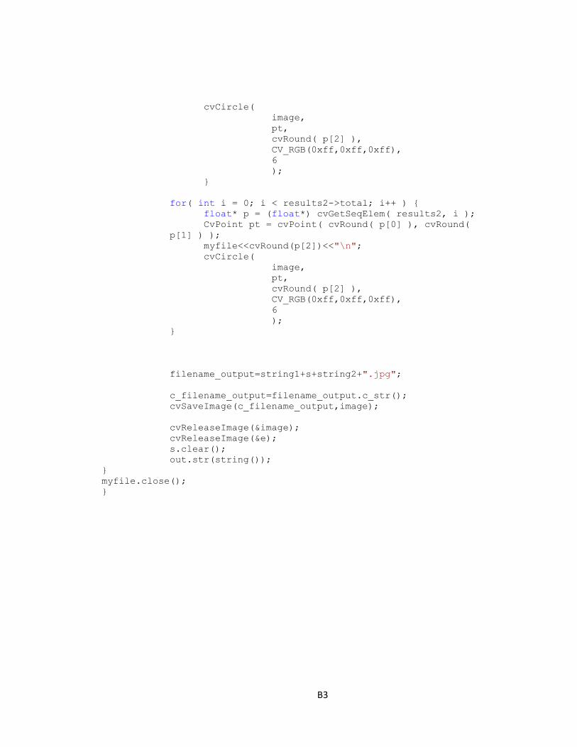
B3
cvCircle(
image,
pt,
cvRound( p[2] ),
CV_RGB(0xff,0xff,0xff),
6
);
}
for( int i = 0; i < results2->total; i++ ) {
float* p = (float*) cvGetSeqElem( results2, i );
CvPoint pt = cvPoint( cvRound( p[0] ), cvRound(
p[1] ) );
myfile<<cvRound(p[2])<<"\n";
cvCircle(
image,
pt,
cvRound( p[2] ),
CV_RGB(0xff,0xff,0xff),
6
);
}
filename_output=string1+s+string2+".jpg";
c_filename_output=filename_output.c_str();
cvSaveImage(c_filename_output,image);
cvReleaseImage(&image);
cvReleaseImage(&e);
s.clear();
out.str(string());
}
myfile.close();
}