LABYRINTH SEAL LEAKAGE ANALYSIS - Texas...
137
LABYRINTH SEAL LEAKAGE ANALYSIS A Thesis by GAURAV CHAUDHARY Submitted to the Office of Graduate Studies of Texas A&M University in partial fulfillment of the requirements for the degree of MASTER OF SCIENCE August 2011 Major Subject: Mechanical Engineering
Transcript of LABYRINTH SEAL LEAKAGE ANALYSIS - Texas...
LABYRINTH SEAL LEAKAGE ANALYSIS
A Thesis
by
GAURAV CHAUDHARY
Submitted to the Office of Graduate Studies of
Texas A&M University
in partial fulfillment of the requirements for the degree of
MASTER OF SCIENCE
August 2011
Major Subject: Mechanical Engineering
LABYRINTH SEAL LEAKAGE ANALYSIS
A Thesis
by
GAURAV CHAUDHARY
Submitted to the Office of Graduate Studies of
Texas A&M University
in partial fulfillment of the requirements for the degree of
MASTER OF SCIENCE
Approved by:
Chair of Committee,
Committee Members,
Head of Department,
August 2011
Major Subject: Mechanical Engineering
Gerald Morrison
J.C. Han
H.C. Chen
Dennis O‟Neal
iii
ABSTRACT
Labyrinth Seal Leakage Analysis.
(August 2011)
Gaurav Chaudhary, B.E., Panjab University
Chair of Advisory Committee: Dr. Gerald L. Morrison
Seals are basic mechanical devices used in machinery to avoid undesired flow
losses of working fluids. Particularly Annular seals are one of the most widely used in
rotating machinery comprising turbines, compressors and pumps. Among all annular
seals straight through rectangular labyrinth seals are the most commonly used ones.
These seals provide resistance to the fluid flow through tortuous path comprising of
series of cavities and clearances. The sharp tooth converts the pressure energy to the
kinetic which is dissipated through turbulence viscosity interaction in the cavity. To
understand the accurate amount of leakage the flow a matrix of fluid flow simulations
carried out using commercially available CFD software Fluent® where all parameters
effecting the flow field has been studied.
The carry over coefficient is found to be a function of the geometry and non-
dimensional flow parameters of the labyrinth seal tooth configuration. Carry over
coefficient increases with tooth clearance, tooth width and Reynolds Number. The
variation with shaft speed does not follow a certain pattern always and varies with shaft
speed.
iv
The discharge coefficient of the first tooth has been found to be lower and
varying in a different manner as compared to a tooth from a multiple cavity seal. The
discharge coefficient of is found to be increasing with increasing tooth width. Rest of the
variation is similar to carry over coefficient variation.
Further the compressibility factor has been defined to incorporate the deviation
of the performance of seals with compressible fluid to that with the incompressible flow.
Its dependence upon pressure ratio and shaft speed has also been established. Using all
the above the mentioned relations it would be easy decide upon the tooth configuration
for a given rotating machinery or understand the behavior of the seal currently in use.

v
DEDICATION
To Spiritual Leader Asaram Bapuji
vi
ACKNOWLEDGEMENTS
I would like to express my sincere thanks to my committee chair, Dr. Gerald L.
Morrison, for the wonderful opportunity of working under his guidance. His exhaustive
knowledge and insight in the field of seals has been a constant source of inspiration and
has provided invaluable assistance during the course of research. I would also like to
express my gratitude to Dr. J. C. Han and Dr. H.C. Chen for being on my thesis
committee and their support.
Special thanks to the Turbo Machinery Research Consortium for partially
funding this research. I am proud to be a part of the Turbo Machinery Laboratory at
Texas A&M University and would like to extend my warm regards to the faculty, staff
and fellow researchers of the Turbo lab.
I thank my parents, sister and uncle for their unfettered support and
encouragement during the entire course of my study. Individual thanks to the department
faculty for making my time at Texas A&M University a wonderful experience.
I‟ve also been fortunate to have a great group of friends at Texas A&M. This
includes my office mates, Anand, Milind, Orcun, Ekene, Vamshi, Shankar, Abhay and
Pranitha. Special thanks go to my many other friends, Vishal, Mohit, Navjit, Ankush,
Aashish, Manish, Narottam and Praveen.
vii
NOMENCLATURE
A - Clearance area, πDc
c - Radial clearance, m
C d - Discharge coefficient for a given tooth
C d1tooth -
Discharge coefficient for first tooth
D – Shaft diameter, m
h – Tooth height, m
L - Axial length of the seal, m
m - Mass flow rate of leakage flow (kg/s)
Pi – Tooth inlet pressure, Pa
Pe - Tooth exit pressure, Pa
Pr – Pressure ratio, pe/pi
Re – Reynolds number based on clearance, m
s - Tooth pitch
w - Tooth width
x - Axial distance along seal, m
α - Flow coefficient
– Divergence angle of jet, radians
γ - Kinetic energy carry over coefficient
– Dissipation of turbulent kinetic energy
viii
– Turbulent kinetic energy
– Dynamic viscosity, Pa/s
ρi – Fluid density at seal inlet, kg/m
3
ρ – Fluid density at tooth inlet, kg/m
3
χ- Percentage of kinetic energy carried over
ψ - Expansion factor
ix
TABLE OF CONTENTS
Page
ABSTRACT ....................................................................................................................... iii
DEDICATION .................................................................................................................... v
ACKNOWLEDGEMENTS ............................................................................................... vi
NOMENCLATURE .......................................................................................................... vii
TABLE OF CONTENTS ................................................................................................... ix
LIST OF FIGURES............................................................................................................xi LIST OF TABLES ............................................................................................................ xv
1. INTRODUCTION ........................................................................................................... 1
2. REVIEW OF CURRENTLY EXISTING LEAKAGE MODELS ................................. 9
3. COMPUTATIONAL FLUID DYNAMICS ................................................................. 16
3.1 Computational Method ........................................................................................... 16 3.2 Governing Equations of Fluid Mechanics .............................................................. 17
3.3 Statistical Turbulence Models ................................................................................ 19 3.3.1 K-ε Turbulence Model ................................................................................ 21
4. RESEARCH OBJECTIVES ......................................................................................... 24
5. COMPUTATIONAL METHOD .................................................................................. 26
6. CARRY OVER COEFFICIENT ................................................................................... 30
6.1 Introduction ............................................................................................................. 30
6.2 Effect of Flow Parameters ....................................................................................... 32 6.2.1 Reynolds Number Variation Effect on the Carry over Coefficient ............... 33
6.3 Effect of Geometrical Parameters on Carry over Coefficient ................................ 36 6.3.1 Effect of Clearance on Carry over Coefficient .................................... 36 6.3.2 Effect of Tooth Width on the Carry over Coefficient .......................... 37
6.3.3 Effect of Pitch on the Carry over Coefficient ...................................... 41 6.3.4 Effect of Shaft Speed Variation on Carry over Coefficient ................. 42
6.4 Cumulative Effect of Changing Various Factors on Carry over Coefficient ......... 52
x
Page
7. DISCHARGE COEFFICIENT ..................................................................................... 58
7.1 First Tooth ............................................................................................................. ..61 7.1.1 Effect of Reynolds Number on Coefficient of Discharge .................... 61 7.1.2 Effect of the Clearance Ratio on Coefficient of Discharge ................. 62 7.1.3 Effect of Tooth Width on Coefficient of Discharge ............................ 63 7.1.4 Effect of Shaft Rotation on Coefficient of Discharge .......................... 66
7.2 Intermediate Tooth of a Multiple Tooth Labyrinth Seal ........................................ 68 7.2.1 Effect of Reynolds Number on Coefficient of Discharge .................... 68
7.2.2 Effect of the Clearance Ratio on Coefficient of Discharge ................ 69 7.2.3 Effect of Tooth Width on Discharge Coefficient ................................. 71 7.2.4 Effect of Shaft Rotation on Discharge Coefficient .............................. 72
7.3 Discharge Coefficient Dependence upon Tooth Position,
W/S, C/S, Ta and Re...............................................................................................75
8. COMPRESSIBILITY FACTOR .................................................................................. .79
8.1 Effect of Position of Tooth on the Compressibility Factor .................................... 81 8.2 Effect of Flow Parameters on Compressibility Factor ........................................... 82 8.3 Effect of Clearance on Compressibility Factor ...................................................... 84 8.4 Effect of Tooth Width on Compressibility Factor ................................................. 85 8.5 Effect of Shaft Rotation on Compressibility Factor ............................................... 86
8.6 Contours of Compressibility Factor ....................................................................... 87
9. SUMMARY........ .......................................................................................................... 97
9.1 Carry over Coefficient ............................................................................................ 97 9.2 Discharge Coefficient ............................................................................................. 97 9.3 Compressibility Factor ........................................................................................... 98
9.4 Suggestible Tooth Configuration ........................................................................... 98
10. RECOMMENDED FUTURE WORK AND CONCLUSION.................................. 100
REFERENCES ................................................................................................................ 102
APPENDIX ..................................................................................................................... 105
VITA...................... ......................................................................................................... 122
xi
LIST OF FIGURES
Page
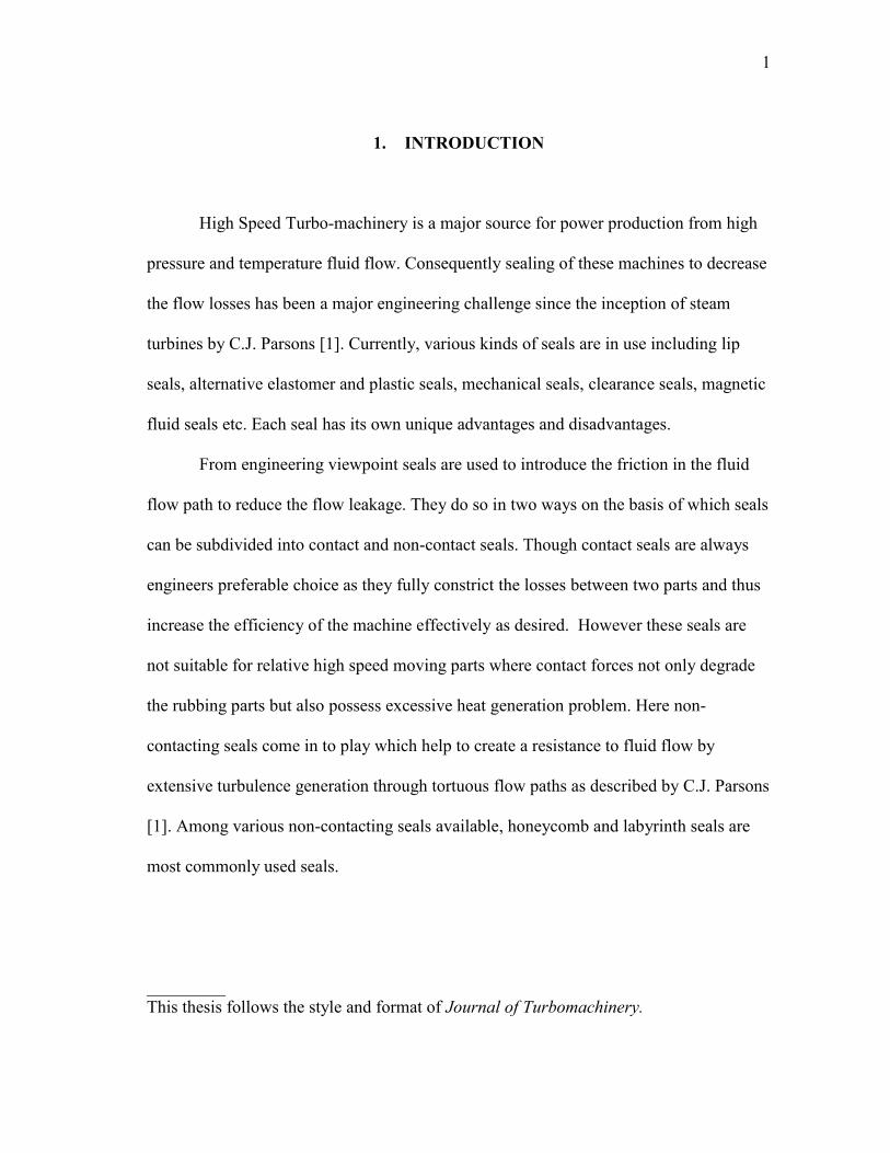
Fig 1.1 Labyrinth seal with tooth on rotor ........................................................................ 2
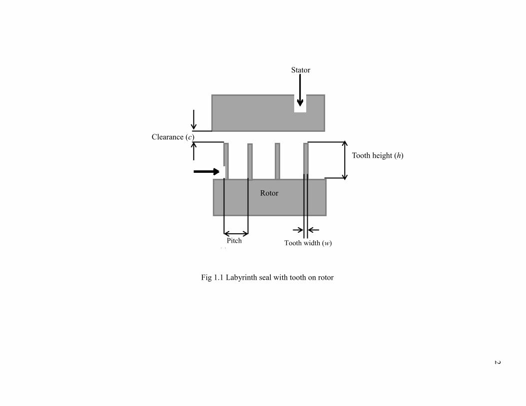
Fig 1.2 Figure sowing energy conversion of energy in labyrinth seal .............................. 3
Fig 1.3 Flow pattern in a labyrinth seal cavity .................................................................. 6
Fig 1.4 Figure showing the relationship between γ and χ ................................................. 7
Fig 5.1 Meshed labyrinth seal geometry ......................................................................... 27
Fig 5.2 Convergence of the simulation with decreasing pressure gradient ..................... 29
Fig 6.1 Streamlines for case with high (Ta/Re) ratio ...................................................... 31
Fig 6.2 Streamlines for case with low (Ta/Re) ratio ....................................................... 31
Fig 6.3 Variation of γ with Re for G4 (Wsh =0, water) ................................................... 33
Fig 6.4 Water case with Re=1000 (G2, Wsh =0) ............................................................. 34
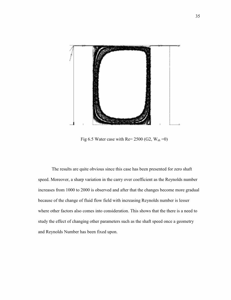
Fig 6.5 Water case with Re= 2500 (G2, Wsh =0) ............................................................ 35
Fig 6.6 Variation of γ with Re for different c/s ratios, water .......................................... 38
Fig 6.7 Variation of γ with Re for different w/s ratios, water ......................................... 40
Fig 6.8 Forces on the fluid in the cavity along the radial direction, First cavity............. 43
Fig 6.9 Variation of γ for cavity 1 with shaft surface speed at Re=1000 ......................... 44
Fig 6.10 Variation of γ for cavity 1 with shaft surface speed at Re=1500 ....................... 45
Fig 6.11 Variation of γ for cavity 1 with shaft surface speed at Re=2000 ....................... 45
Fig 6.12 Variation of γ for cavity 1 with shaft surface speed at Re=2300 ....................... 46
Fig 6.13 Variation of γ for cavity 1 with shaft surface speed at Re=2500 ....................... 46
Fig 6.14 Pressure difference variation with shaft speed (G1& Re=1000) ....................... 47
xii
Page
Fig 6.15 Variation of forces with shaft speed (Not to scale) ............................................ 48
Fig 6.16 Variation of γ for cavity 1 with shaft surface speed for G4 ............................... 49
Fig 6.17 Variation of γ for cavity 1 with shaft surface speed for G4 ............................... 50
Fig 6.18 Variation of γ for cavity 1 with shaft surface speed for G4 ............................... 50
Fig 6.19 Variation of γ for cavity 1 with shaft surface speed for G4 ............................... 51
Fig 6.20 Variation of γ for cavity 1 with shaft surface speed for G4 ............................... 51
Fig 6.21 γ changes with Ta, Re and C/S for W/S =0.25 (G2, G3 & G5) ......................... 53
Fig 6.22 γ changes with Ta, Re and C/S for W/S =0.0075 (G1 & G4) ............................ 54
Fig 6.23 Mean flow streamlines for Re=10000 at Wsh =0 for G4 .................................... 55
Fig 6.24 Mean flow streamlines for Re=10000 at Wsh =350m/s for G4 .......................... 56
Fig 7.1 Carry over coefficient calculation points ............................................................ 59
Fig 7.2 Variation of Cd with tooth (Water, G4, Re=2000,Wsh =0) ................................. 60
Fig 7.3 Variation of Cd1tooth
with Re (Water, G3, 0 RPM) .............................................. 61
Fig 7.4 Variation of coefficient of discharge with Re for different c/s ratio ................... 62
Fig 7.5 Variation of coefficient of discharge with Re for different w/s ratio.................. 64
Fig 7.6 Streamlines for G1 ( Wsh =0 & Re=2000) .......................................................... 65
Fig 7.7 Streamlines for G2 ( Wsh =0 & Re=2000) .......................................................... 65
Fig 7.8 Variation coefficient of discharge for different shaft surface speeds ................. 66
Fig 7.9 Streamlines upstream of first tooth for Wsh =0 for G2 and Re=2000 ................. 67
Fig 7.10 Streamlines upstream of first tooth for Wsh =350 for G2 and Re=2000 ............ 67
Fig 7.11 Variation of Cd with Re, G3 (tooth2, water) ...................................................... 68
xiii
Page
Fig 7.12 Variation of Cd with Re for different c/s ratio (tooth2, water) ........................... 70
Fig 7.13 Variation of Cd with Re for different w/s ratio (tooth2, water) ......................... 72
Fig 7.14 Variation Cd for different shaft speed, G2 (tooth2, water, Re=2000) ................ 73
Fig 7.15 Mean flow streamlines for Re=2000 at Wsh =0 for G2, tooth 2......................... 74
Fig 7.16 Mean flow streamlines for Re=2000 at Wsh =350m/s for G2, tooth 2 ............... 74
Fig 7.17 Cd changes for Ta, Re and C/S for W/S =0.25 (G2, G3 & G5) ......................... 76
Fig 7.18 Cd changes for Ta, Re and C/S for W/S =0.0075 (G1 & G4) ............................ 77
Fig 8.1 Variation of discharge coefficients at different pressure ratios .......................... 80
Fig 8.2 Variation of compressibility factor with tooth position ...................................... 82
Fig 8.3 Variation of compressibility factor with pressure ratio ...................................... 83
Fig 8.4 Variation of compressibility factor with c/s ratio ............................................... 84
Fig 8.5 Effect of compressibility factor with w/s ratio ................................................... 85
Fig 8.6 Effect on compressibility factor with shaft speed ............................................... 86
Fig 8.7 Contour of ψ for Re=1000, G1 ........................................................................... 87
Fig 8.8 Contour of ψ for Re=1500, G1 ........................................................................... 88
Fig 8.9 Contour of ψ for Re=2000, G1 ........................................................................... 88
Fig 8.10 Contour of ψ for Re=500, G2 ............................................................................ 89
Fig 8.11 Contour of ψ for Re=1000, G2 .......................................................................... 89
Fig 8.12 Contour of ψ for Re=1500, G2 .......................................................................... 90
Fig 8.13 Contour of ψ for Re=1000, G3 .......................................................................... 90
Fig 8.14 Contour of ψ for Re=2000, G3 .......................................................................... 91
xiv
Page
Fig 8.15 Contour of ψ for Re=1000, G4 .......................................................................... 91
Fig 8.16 Contour of ψ for Re=2000, G4 .......................................................................... 92
Fig 8.17 Contour of ψ for Re=5000, G4 .......................................................................... 92
Fig 8.18 Contour of ψ for Re=1000, G5 .......................................................................... 93
Fig 8.19 Contour of ψ for Re=2000, G5 .......................................................................... 93
Fig 8.20 Contour of ψ for Re=5000, G5 .......................................................................... 94
Fig A.1 γ changes with Ta, Re and C/S for W/S =0.25 (G2, G3 & G5) ....................... 105
Fig A.2 γ changes with Ta, Re and C/S for W/S =0.0075 (G1 & G4) .......................... 106
Fig A.3 γ changes with Ta, Re and C/S for W/S =0.25 (G2, G3 & G5) ....................... 107
Fig A.4 γ changes with Ta, Re and C/S for W/S =0.0075 (G1 & G4) .......................... 108
Fig A.5 Cd changes for Ta, Re and C/S for W/S =0.25 (G2, G3 & G5) ....................... 109
Fig A.6 Cd changes for Ta, Re and C/S for W/S =0.0075 (G1 & G4) .......................... 110
Fig A.7 Cd changes for Ta, Re and C/S for W/S =0.25 (G2, G3 & G5) ....................... 111
Fig A.8 Cd changes for Ta, Re and C/S for W/S =0.0075 (G1 & G4) .......................... 112
Fig A.9 Cd changes for Ta, Re and C/S for W/S =0.25 (G2, G3 & G5) ....................... 113
Fig A.10 Cd changes for Ta, Re and C/S for W/S =0.0075 (G1 & G4) ......................... 114
Fig A.11 Variation of pressure ratio across seal ............................................................ 118
Fig A.12 Variation of pressure ratio across seal ............................................................ 119
Fig A.13 Large teeth geometry ...................................................................................... 120
Fig A.14 Small teeth geometry ...................................................................................... 120
xv
LIST OF TABLES
Page
Table 1 Variation of Cavity Forces .................................................................................. 43
Table 2 Effect of Tooth Width and c/s on Carry over Coefficient ................................... 56
Table 3 Reynolds Number and Shaft RPM used for simulation ...................................... 57
Table 4 γ variation with C/S and tooth width ................................................................... 78
Table 5 Cd and γ variation with c/s ratio .......................................................................... 99
Table 6 Seal geometries used for simulation ................................................................. 115
Table 7 ∆P ( Pascal) variation with shaft surface speed Wsh (m/s) ............................... 116
1
1. INTRODUCTION
High Speed Turbo-machinery is a major source for power production from high
pressure and temperature fluid flow. Consequently sealing of these machines to decrease
the flow losses has been a major engineering challenge since the inception of steam
turbines by C.J. Parsons [1]. Currently, various kinds of seals are in use including lip
seals, alternative elastomer and plastic seals, mechanical seals, clearance seals, magnetic
fluid seals etc. Each seal has its own unique advantages and disadvantages.
From engineering viewpoint seals are used to introduce the friction in the fluid
flow path to reduce the flow leakage. They do so in two ways on the basis of which seals
can be subdivided into contact and non-contact seals. Though contact seals are always
engineers preferable choice as they fully constrict the losses between two parts and thus
increase the efficiency of the machine effectively as desired. However these seals are
not suitable for relative high speed moving parts where contact forces not only degrade
the rubbing parts but also possess excessive heat generation problem. Here non-
contacting seals come in to play which help to create a resistance to fluid flow by
extensive turbulence generation through tortuous flow paths as described by C.J. Parsons
[1]. Among various non-contacting seals available, honeycomb and labyrinth seals are
most commonly used seals.
_________
This thesis follows the style and format of Journal of Turbomachinery.
2
Rotor
Stator
Clearance (c)
Tooth
Pitch
(s)
Tooth height (h)
Tooth width (w)
Fig 1.1 Labyrinth seal with tooth on rotor
3
Upstream pressure
converted to velocity.
Final expansion
to exit pressure.
Upstream
Tooth
The jet causes recirculating flow in
the intervening cavity which
dissipates energy.
Downstream Tooth
Axis of Rotation
Jet Created by
constriction expands into
intervening cavity.
Portion of jet gets “carried
over” to next throttling.
PEXIT
< PO
PO
Fig 1.2 Figure sowing energy conversion of energy in labyrinth seal
4
Further labyrinth seals could be subdivided in to straight, stepped and staggered
seals. On the basis of the tooth profile another sub-division could be done. Among all the
above discussed seals straight through rectangular tooth labyrinth seals are the most
popular type due to the ease manufacturing and effective sealing properties. These seals
consist of a series of rectangular teeth over the length of a span of turbine blades or on
the rotating shaft with cavities in between to dissipate the energy of fluid flow leakage as
is shown in Figure 1.1. The sharp tooth clearance in geometry helps to increase the
kinetic energy of the fluid flow by throttling and converting pressure energy to kinetic
energy. Additionally it also create losses by generation of eddies and vena contracta
effect. Further in the cavities fluid dissipate kinetic energy through turbulence-viscosity
interaction. This has been shown in Figure 1.2. Thus effectively a labyrinth creates 3-D
vortices in each chamber between two constrictions going all around the circumference
of the rotating machinery.
Mathematically for the steady state operation of a Turbine (fixed RPM) the
governing equations produce an elliptic problem with the governing equations described
by basic conservation laws from thermal and fluid flow sciences. Due to this nature of
the problem, various factors (geometry, flow and operating conditions) which constitute
the boundary conditions need to be studied to determine the effect of each on the fluid
flow leakage. The geometry of the labyrinth seal flow being one of those prominent
parameters. Among various other factors affecting the labyrinth seal leakage are the
fluid flow boundary conditions and the relative movement of the shaft.
5
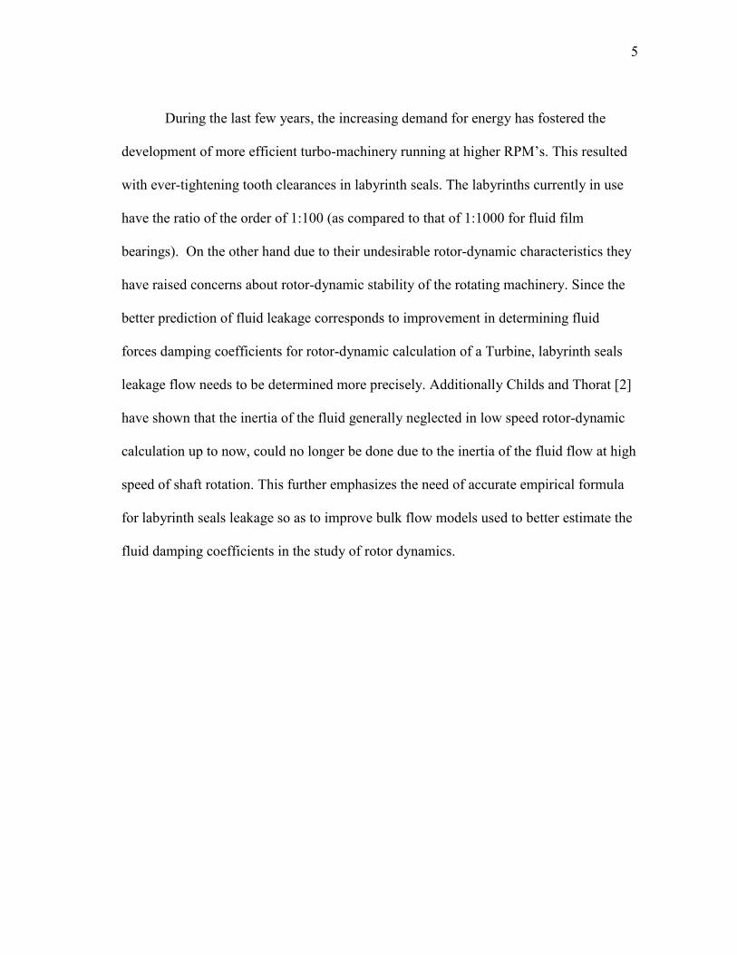
During the last few years, the increasing demand for energy has fostered the
development of more efficient turbo-machinery running at higher RPM‟s. This resulted
with ever-tightening tooth clearances in labyrinth seals. The labyrinths currently in use
have the ratio of the order of 1:100 (as compared to that of 1:1000 for fluid film
bearings). On the other hand due to their undesirable rotor-dynamic characteristics they
have raised concerns about rotor-dynamic stability of the rotating machinery. Since the
better prediction of fluid leakage corresponds to improvement in determining fluid
forces damping coefficients for rotor-dynamic calculation of a Turbine, labyrinth seals
leakage flow needs to be determined more precisely. Additionally Childs and Thorat [2]
have shown that the inertia of the fluid generally neglected in low speed rotor-dynamic
calculation up to now, could no longer be done due to the inertia of the fluid flow at high
speed of shaft rotation. This further emphasizes the need of accurate empirical formula
for labyrinth seals leakage so as to improve bulk flow models used to better estimate the
fluid damping coefficients in the study of rotor dynamics.
6
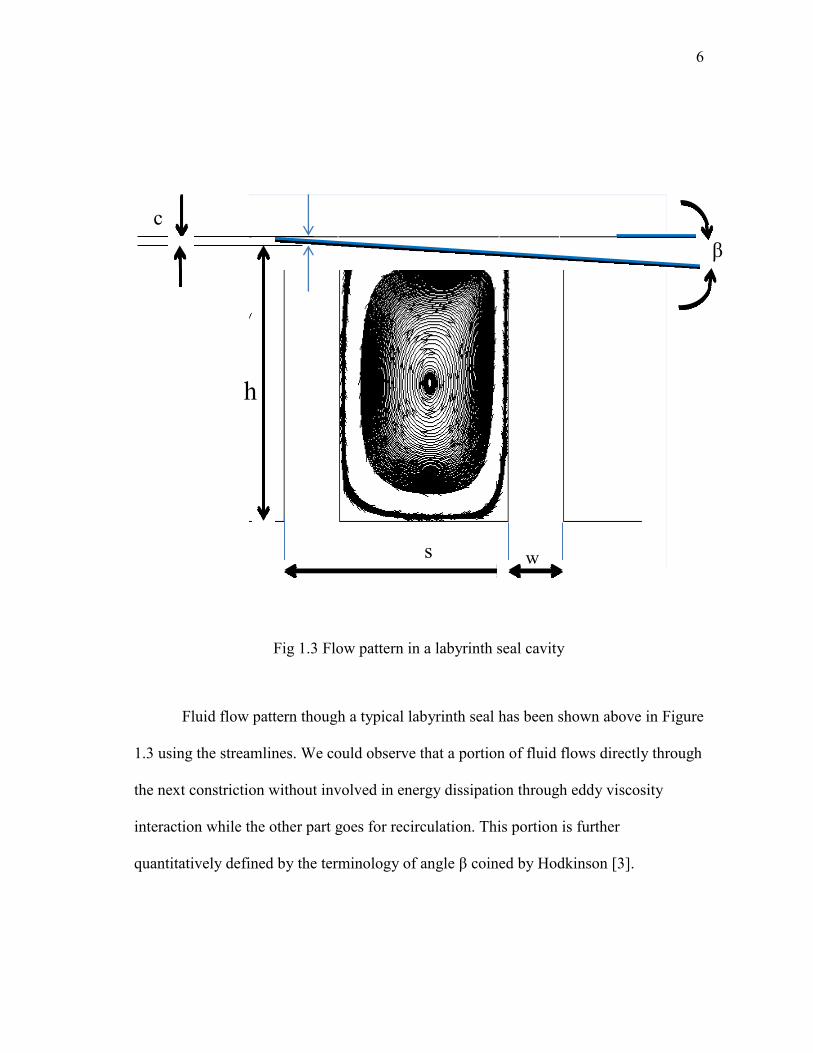
Fig 1.3 Flow pattern in a labyrinth seal cavity
Fluid flow pattern though a typical labyrinth seal has been shown above in Figure
1.3 using the streamlines. We could observe that a portion of fluid flows directly through
the next constriction without involved in energy dissipation through eddy viscosity
interaction while the other part goes for recirculation. This portion is further
quantitatively defined by the terminology of angle β coined by Hodkinson [3].
β
h
c
s w
7
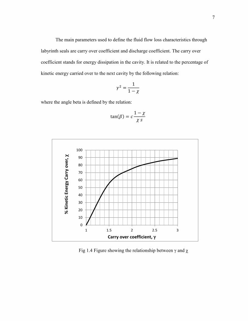
The main parameters used to define the fluid flow loss characteristics through
labyrinth seals are carry over coefficient and discharge coefficient. The carry over
coefficient stands for energy dissipation in the cavity. It is related to the percentage of
kinetic energy carried over to the next cavity by the following relation:
where the angle beta is defined by the relation:
( )
Fig 1.4 Figure showing the relationship between γ and χ
0
10
20
30
40
50
60
70
80
90
100
1 1.5 2 2.5 3
% K
inet
ic E
ner
gy C
arry
ove
r, χ
Carry over coefficient, γ
8
From the Figure 1.4 it is clear that the ideal value of carry over coefficient should
be 1 which denoted the complete dissipation of the energy in the cavity. As the value of
the angle beta goes higher than lesser is the dissipation of the energy. The discharge
coefficient as usually denoted defines the flow losses through each constriction. It is
somehow similar to the flow losses through the orifice plate but not exactly same due to
the flow conditions being much different.
9
2. REVIEW OF CURRENTLY EXISTING LEAKAGE MODELS
The first paper to describe the labyrinth fluid flow was by Becker [4]. He
modeled the fluid flow through labyrinth seals as Poiseuille flow with an attempt to find
a coefficient of friction as to treat the flow as a simple annular flow. He observed that
smaller decrease in clearance has a greater effect rather than changing the fluid flow path
by varying tooth and cavity geometry.
Shortly after Becker [4] in another pioneering paper in 1908, Martin [5] proposed
to treat the problem in an entirely different manner by considering labyrinth seals as a
series of throttling process similar to the flow through a series of orifices. His approach
was purely analytical with various false assumptions. He treated the pressure drop to be
linearly varying and flow to be isothermal. Additionally he assumed the pressure across
each constriction (tooth) to be very small or treated that the flow was always in sub-
critical state throughout the labyrinth seal. He did not compare his equations against any
experimental data. In the subsequent papers mostly all authors tried to address the wrong
assumptions made by Martin [5] and improved his formulae.
Stodola [6] in his book on steam and gas turbines considered flow leakage
through staggered and radial seals. He presented two separate equations to calculate flow
leakage one each for subsonic and sonic respectively. He presented the experimental
results on interlocking seals with clearances varying from 0.14 mm to 0.38 mm and
pressure ranging from 43 to 143 psi. He carried out his experiments with a non-rotating
shaft and thus neglected effects of shaft rotation on fluid flow leakage. He also assumed
10
that kinetic energy gets completely dissipated in the cavity and neglected the kinetic
energy carry over coefficient. This leaded to a variation of about 14% in his formulas for
calculating flow leakages. Additionally he also developed a graphical method for
analyzing seals with varying areas those found in radial labyrinths.
Dollin and Brown [7] derived the Martin [5] analytical formulae for calculating
the flow through labyrinth seals. They assumed the thermodynamic path function to be
polytrophic (pvk
= constant) rather than isothermal and derived more general formula for
fluid flow leakage. Martin leakage equation was a special case of their formula with k=1
and for the incompressible flow its value reduced to be k=∞. They also neglected the
kinetic energy carry over coefficient.
Gercke [8] derived his equation by considering the variable area. He gave
importance to kinetic energy carry over between throttling. He assumed that the flow
through flow through each throttling was adiabatic and that through each cavity is
isothermal with constant pressure process. He also took into consideration the
occurrence of vena contracta and defined discharge coefficient but neglected the shaft
rotation.
Elgi [9] made another major contribution to the fluid flow through labyrinth seals
through his paper on labyrinth seals in 1935. He examined both staggered and see-
through configuration of labyrinth seals theoretically and experimentally. His
experiments included study for clearances in range of 15 to 40 mils. He used the same
formula as stated by Martin [5] but used took in to consideration the occurrence of vena
contract as the fluid goes through tooth clearances. He also considered the kinetic energy
11
carry over coefficient by defining a “carry-over” factor which he determined
experimentally. Through experimental results and analytical study he also noticed that
kinetic energy carry over coefficient decreases with increasing pitch between
constrictions or by decreasing clearances. This effect could be attributed to the increases
in the expansion of the jet emerging from tooth clearance in the subsequent cavity due to
the above two factors. In non-dimensional he mentioned the result as a ratio clearance–
to-pitch ratio. The variation of discharge coefficient with the variation of pressure ratio
was also observed.
Keller [10] through his experiments analyzed the leakage quantitatively. He did
experiments on flow of water and air through labyrinth seals. His results showed how the
interlocking blade configuration has much better sealing properties as compared to see
through seals. He neglected the effect of shaft rotation on the fluid flow and conducted
tests in a non-rotating test rig having rectangular and rounded shape blades with
clearances in the form of long rectangular strips rather than annuli.
Hodkinson [3] analyzed the leakage problem analytically rather than
experimentally. He stated that a portion of jet leaving the clearances was intercepted by
the next clearance without any energy loss. He defined this portion of fluid by using a
parameter beta (β). He took this effect in to consideration in the Stodola equation for
orifice coefficient. He also discussed the effects of eccentricity and rotational speed on
seal leakage. From the results of his experiments he showed that eccentricity is more
pronounces in laminar flow than in case of turbulent flow where flow could increase up
to 2.5 times. His study included low RPM (not true for modern turbo machinery realm
12
where shaft speed could go up to supersonic) of machines where he showed that rotating
shaft has nominal difference on leakage of fluid as compared to a stationary shaft from
viewpoint of labyrinth seal leakage.
Bell and Bergin [11] assumed that the labyrinth seal constrictions to follow the
flow field as through annular orifices. They mentioned few interesting observations
made during experiments done on orifice meter. They mainly divided the fluid flow in
two main categories based on the Reynolds number. For the lower Reynolds molecular
viscosity is the main cause of losses for fluid flow. While for the high Reynolds number
turbulent viscosity is the major factor to be considered responsible for fluid flow losses.
An equation to take into consideration the eccentricity of the shaft is also mentioned by
them. It was also observed that undesirable recovery of kinetic energy to pressure energy
(reverse of throttling process) occurs for turbulent flow through thicker orifices but it
does not occur smooth orifices. Further for higher Reynolds number flow wall friction
factor also comes into play for thick orifices or wider tooth of labyrinth constriction.
From the experimental readings for high Reynolds number it was claimed that
undesirable pressure recovery due to the occurence of vena contracta starts from
thickness-to-clearance (w/c) ratio of 1 and increases up to 6. Further increasing thickness
makes wall friction to be more dominant and which reduces the flow leakage by creating
pressure losses through shear stress losses at the boundaries of labyrinth tooth clearance
flow field. Contrastingly for low Re flow pressure recovery does and occurs and only
wall helps to create a pressure loss.
13
Kearton and Keh [12] performed experiments on single orifice with zero initial
velocity. They determined the effects of pressure ratios on discharge coefficient. They
also accounted for the compressibility of the fluid flow and used that in the correction
for the for the leakage flow developed by Martin. However they neglected the kinetic
energy carry over coefficients and avoided the rotation effect of the shaft on the fluid
flow leakage. They did performed tests on a 14 throttle staggered labyrinth seals where
their analytical formulae performed predicted flow leakage with a fair accuracy.
Zabriskie and Sternlicht [13] performed investigation on straight tooth labyrinth
seals. They did not perform any experiments but used data gathered from previous
studies. Their basic approach was to determine a friction factor and later correlate it with
the seal geometry, mass flow rate and pressure ratio.
Heffener [14] use the formula given by Martin [5] and found the value of
empirical data for Coefficient of discharge to take in to consideration the effects of wall
losses and flow contraction at the throttling of the constriction. His neglected the kinetic
energy carry over coefficient and the rotation effect of the shaft.
Komotri and Mori [15] treated the flow through constriction as adiabatic and
entire leakage as isoenthalpic. They had n equations for n constrictions. These equations
were solved together for finding the final function which is a function of carryover
coefficient, number of teeth and thermodynamic process coefficient.
Rao and Narayanamurthi [16] took in to account the rotation of the shaft in their
study of labyrinth seals. They performed experiments on two geometries: (1) 40 teeth
seal with a pitch of 5 mm, (2) 20 teeth seal with pitch of 10 mm on a see through
14
labyrinth seals. The results from their experiments indicated that for a pressure ration in
the range of 0.15 to 0.6 the leakage increases till the speed of 1100 rpm and decreases
afterwards. This increment in the leakage was 4% for the 40 teeth as compared to the 10%
increase for 20 teeth geometry.
From his investigations on labyrinth seals Stocker revealed the following facts
about labyrinth seals. The data from his studies indicate that leakage decreased up to
certain limit of surface roughness further roughness would tend to increase the flow
leakage. Also he noticed that rotation of the shaft could affect the leakage up to 10%.
Further he concluded that somewhere in between 50 to 70 degrees tooth angle leakage
was minimum and pitch decreases for minimum leakage decreases with increasing tooth
angle.
Deych [17] studied seals for steam turbine turbines. He conducted two
experimental studies. In the first study he calculated leakage through seals as a function
of pressure ratio and quality of steam. He did not consider the carry over coefficient for
kinetic energy and for the kinetic energy carried over the next cavity.
Vermes [18] covered all the issues that were either missing or lacking in the
previous papers discussed above. Martin‟s formula was adjusted for non-isothermal fluid
flow with flow coefficients adopted from Bell and Berglein [11]. A further major
correction was derived by considering boundary layer theory of Schiliting [19] in the
kinetic energy carry over coefficient. His flow coefficient is a function of pitch, tooth
width and clearance. His equations varied from experimental results by 5%.
15
Ahmed Gamal [20] further analyzed the above mentioned models and showed
the variation of kinetic energy carry over coefficient. These results showed the
fundamental dependence of the leakage problem upon factors other than geometry of
labyrinth seals as expected from the elliptic nature of the governing equations for steady
state flow.
Saikishan [21] discussed in his thesis how the variations of flow defining
parameters are related to changing fluid flow characteristics. He did not consider the
tooth on the rotating shaft seal nor the effect of that on the kinetic energy carry over
coefficient.
16
3. COMPUTATIONAL FLUID DYNAMICS
3.1 Computational Method
The current research work is done using CFD simulations of fluid flow through
labyrinth seals. The effect of rotation of shaft on the flow pattern through seals is studied
by varying the shaft surface velocity from zero to slightly above Mach 1. Apart from this
the effect of geometric shapes of the labyrinth seal geometry is also being studied while
keeping tooth height to pitch ratio as 1 and varying another geometrical parameters.
There are few assumptions made which have helped to reduce the computational effort
in terms of time for the current research. These assumptions are:
1) The flow is axisymmetric which have helped to reduce the flow from three
dimensional to two dimensional.
2) The variations in the shapes of the geometry of metal (due to thermal and fatigue
stress) defining the fluid flow path is negligible compared to the length of the tooth
clearances.
3) Fluid Surface interaction (FSI) has not been taken in to consideration to take into
account the surface roughness of the seal geometry. Also impact of lateral surface
vibrations due to dynamics of rotating shaft have not been considered to do negligible
contribution to fluid turbulence intensity.
For the current turbulent flow simulations commercial solver FLUENT® has
been employed to solve the fundamental governing equations of thermo-fluid sciences.
The partial differential equation have been discretized using Finite-Volume Method and

17
turbulence flow modeled using standard k-ε turbulence model along with enhanced wall
function in the near wall region flow to resolve viscous sub-layer without additional
effort in terms of more refined mesh. The choices of current turbulence model to
simulate the current fluid flow have been verified by Morrison and Al-Ghasem [22] by
comparison with experimental LDA data by Morrison and Johnson [23]. More
mathematical details about these models and wall function could be found in the
following subsections.
Grid independence study was performed was using refined mesh till the outlet
pressure difference value across the seal value stabilizes with increasing grid resolution
for a given mass inlet flow rate and pressure at the inlet. Adaption of grid was based on
pressure gradient set to a maximum value of 1 and Y+ set as 5.
3.2 Governing Equations of Fluid Mechanics
The governing equations of fluid mechanics include the conservation laws for
mass, momentum, and energy, which are usually, expressed using the Eulerian
description. Mechanical and thermodynamic property constitutive equations are needed
to close the close these system of equations. The momentum conservation law for
Newtonian fluids is also known as the Navier–Stokes equations, where the stress tensor
T is given by:
(p
)
18
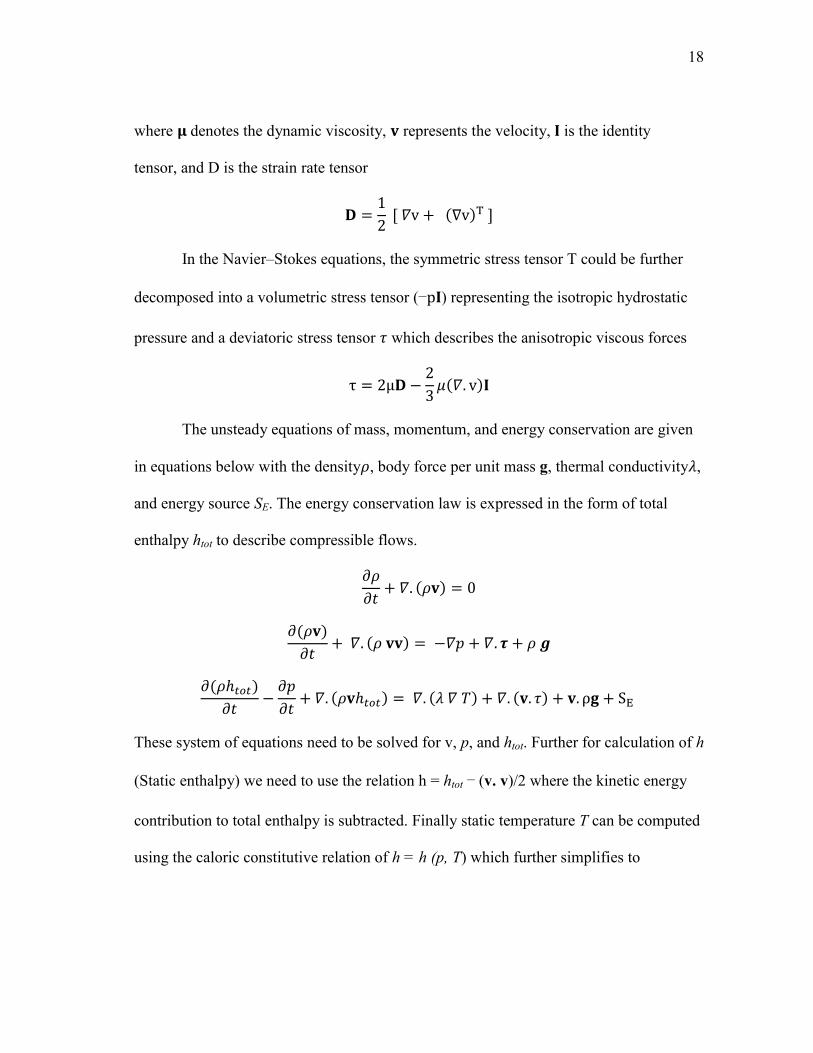
where denotes the dynamic viscosity, represents the velocity, is the identity
tensor, and D is the strain rate tensor
( )
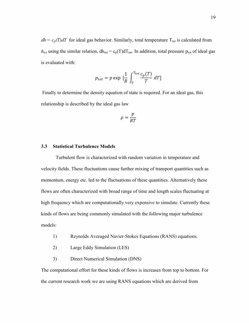
In the Navier–Stokes equations, the symmetric stress tensor T could be further
decomposed into a volumetric stress tensor (−p ) representing the isotropic hydrostatic
pressure and a deviatoric stress tensor which describes the anisotropic viscous forces
( )
The unsteady equations of mass, momentum, and energy conservation are given
in equations below with the density , body force per unit mass g, thermal conductivity ,
and energy source SE. The energy conservation law is expressed in the form of total
enthalpy htot to describe compressible flows.
( )
( )
( )
( )
( ) ( ) ( ) ρ
These system of equations need to be solved for v, p, and htot. Further for calculation of h
(Static enthalpy) we need to use the relation h = htot − (v. v)/2 where the kinetic energy
contribution to total enthalpy is subtracted. Finally static temperature T can be computed
using the caloric constitutive relation of h = h (p, T) which further simplifies to
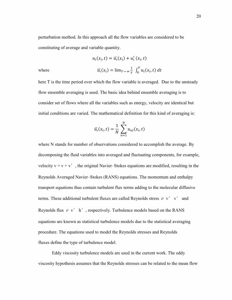
19
dh = cp(T)dT for ideal gas behavior. Similarly, total temperature Ttot is calculated from
htot using the similar relation, dhtot = cp(T)dTtot. In addition, total pressure ptot of ideal gas
is evaluated with:
p
∫
( )
Finally to determine the density equation of state is required. For an ideal gas, this
relationship is described by the ideal gas law
3.3 Statistical Turbulence Models
Turbulent flow is characterized with random variation in temperature and
velocity fields. These fluctuations cause further mixing of transport quantities such as
momentum, energy etc. led to the fluctuations of these quantities. Alternatively these
flows are often characterized with broad range of time and length scales fluctuating at
high frequency which are computationally very expensive to simulate. Currently these
kinds of flows are being commonly simulated with the following major turbulence
models:
1) Reynolds Averaged Navier-Stokes Equations (RANS) equations.
2) Large Eddy Simulation (LES)
3) Direct Numerical Simulation (DNS)
The computational effort for these kinds of flows is increases from top to bottom. For
the current research work we are using RANS equations which are derived from
20
perturbation method. In this approach all the flow variables are considered to be
constituting of average and variable quantity.
( ) ( ) ( )
where ( ) im
∫ ( )
here T is the time period over which the flow variable is averaged. Due to the unsteady
flow ensemble averaging is used. The basic idea behind ensemble averaging is to
consider set of flows where all the variables such as energy, velocity are identical but
initial conditions are varied. The mathematical definition for this kind of averaging is:
( )
∑ ( )
where N stands for number of observations considered to accomplish the average. By
decomposing the fluid variables into averaged and fluctuating components, for example,
velocity v = v + v′, the original Navier–Stokes equations are modified, resulting in the
Reynolds Averaged Navier–Stokes (RANS) equations. The momentum and enthalpy
transport equations thus contain turbulent flux terms adding to the molecular diffusive
terms. These additional turbulent fluxes are called Reynolds stress ρ v′ v′ and
Reynolds flux ρ v′ h′, respectively. Turbulence models based on the RANS
equations are known as statistical turbulence models due to the statistical averaging
procedure. The equations used to model the Reynolds stresses and Reynolds
fluxes define the type of turbulence model.
Eddy viscosity turbulence models are used in the current work. The eddy
viscosity hypothesis assumes that the Reynolds stresses can be related to the mean flow

21
and turbulent viscosity µt in a manner analogous to molecular viscosity µ in laminar
flows. In other words, the turbulent effect can be represented as an increased viscosity
with the effective viscosity µeff = µ+µt.
3.3.1 K-ε Turbulence Model
It is a type of eddy viscosity model based on analogy between laminar and
turbulent flows based on Boussinesq hypothesis. The central idea of this model is that
turbulent flow stresses behave similar to laminar fluid stresses which follow stokes law.
Mathematically it could be written as:
{
(
)
{
(
)
Here:
1) = Turbulent Viscosity
2) k = Turbulent Kinetic Energy
3) kt = Turbulent conduction effect
22
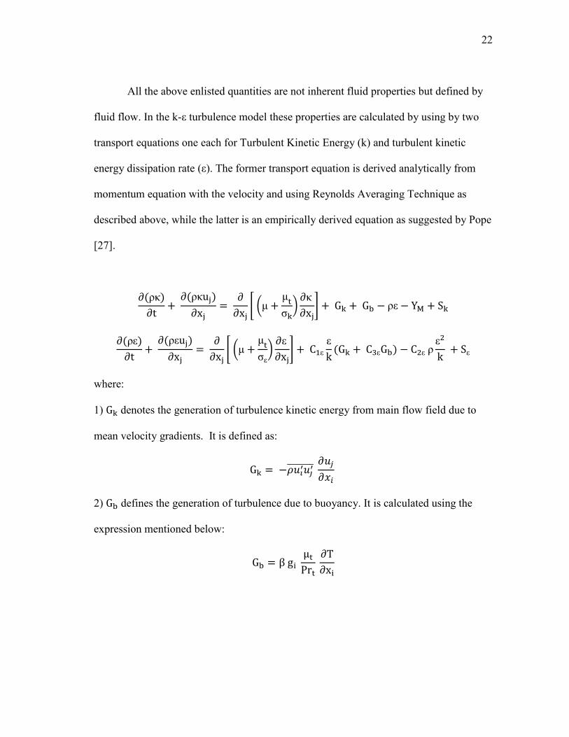
All the above enlisted quantities are not inherent fluid properties but defined by
fluid flow. In the k-ε turbulence model these properties are calculated by using by two
transport equations one each for Turbulent Kinetic Energy (k) and turbulent kinetic
energy dissipation rate (ε). The former transport equation is derived analytically from
momentum equation with the velocity and using Reynolds Averaging Technique as
described above, while the latter is an empirically derived equation as suggested by Pope
[27].
( )
( )
* (
)
+ ε
( ε)
( ε )
* (
ε)
ε
+ ε
ε
( ε ) ε
ε
ε
where:
1) denotes the generation of turbulence kinetic energy from main flow field due to
mean velocity gradients. It is defined as:
2) defines the generation of turbulence due to buoyancy. It is calculated using the
expression mentioned below:
i
P
i
23
3) represents the contribution by dilation to the overall dissipation rate in
compressible fluid flow. It is calculated using the expression below:
ρ
4) ς and ς are the turbulent Prandtl numbers for and , and have default values of 1.0
and 1.3 respectively. and are constants with default values of 1.44 and 1.92. For
this research these default values have been used.
24
4. RESEARCH OBJECTIVES
This work is aimed at understanding the effect of different parameters on the
fluid flow leakage through labyrinth seals with the tooth mounted on the rotor. As
mentioned earlier in this study we will explore the labyrinth tooth rectangular in shape
and mounted on rotor. This study deals with exploring the effect of all the variables
(including the flow parameters, geometry dimensions and moving boundaries) suspected
to determine the carry over coefficients and discharge coefficients of a given labyrinth
seal under consideration. Broadly it could be said that it comprises of the following main
three tasks.
Firstly effect of flow parameters on the carry over coefficient was studied. This is
done in a procedural manner starting from the effect of non-dimensional flow field
parameter i.e. Reynolds Number. It is calculated for the current research study using the
formulae mentioned below.
Further from this relation we conclude that, for a give shaft diameter
Also since
So from using the above mentioned two equations we deduce that:
or
25
To explore the effect of Reynolds number same geometry (at a given shaft RPM)
is considered at different Reynolds Numbers. After that, the effect of geometrical
parameters including the tooth clearance to the pitch (c/s) ratio and the effect of tooth
width to pitch (w/s) is studied. Both these calculations are achieved by choosing
different cases with same geometrical lengths (except clearances and tooth width) are
studied for different Reynolds Numbers. Finally, effect of shaft RPM on the carry over
coefficient was studied by varying the shaft speed for fixed Reynolds number and
geometry.
Secondly, the effect of various parameters on discharge coefficient was evaluated
using the same procedure as above. Here, the study mainly bifurcated into two different
cases 1) for the first tooth of labyrinth seal 2) for the tooth having cavity prior to them.
This division was done after considering the difference in the discharge coefficient of
first teeth from the rest of the labyrinth seal tooth.
The third task comprised of determining the effect of various conditions
considered above on the expansion factor. This factor is introduced to predict the
deviation in the behavior of seals with compressible fluid as compared to the one with
incompressible fluids.
26
5. COMPUTATIONAL METHOD
The current research work has chosen the path of CFD methodology to study the
Labyrinth seal fluid flow. Further, in the present study the flow field has been simplified
from three dimensional to axisymmetric two dimensional. This replication of 3D leakage
characteristics from 2D turbulent flow within acceptable accuracy has been proven by
various other research studies including that by Stoff [24] on labyrinth seals. This saves
considerable time and effort required for expensive experimental methods. These
simulations are used primarily to study the factors affecting kinetic energy carry over
coefficient and discharge coefficient for the fluid flow leakage through labyrinth seals.
Furthermore, various others factors have been studied to show their variance with the
changing geometrical and fluid conditions.
Fluent® is finite volume discretization based CFD solver used lot solve the
Navier Stokes simulation. For this study, standard k-ε turbulence model has been used to
solve the turbulent fluid flow field. The applicability of this model to accurately simulate
the flow field has been studied by Morrison and Al-Ghasem [22]. The study mentions
the similarity between labyrinth seal flow patterns obtained using k-ε modeling and the
experimental data from Laser Doppler Anemometry (LDA) performed by Morrison and
Johnson [23]. More details about the turbulence modeling have been mentioned in the
previous section.
Gambit has been used as a preprocessor to generate the meshes required for the
current simulations. Rectangular grid cells have been used for the current flow field as
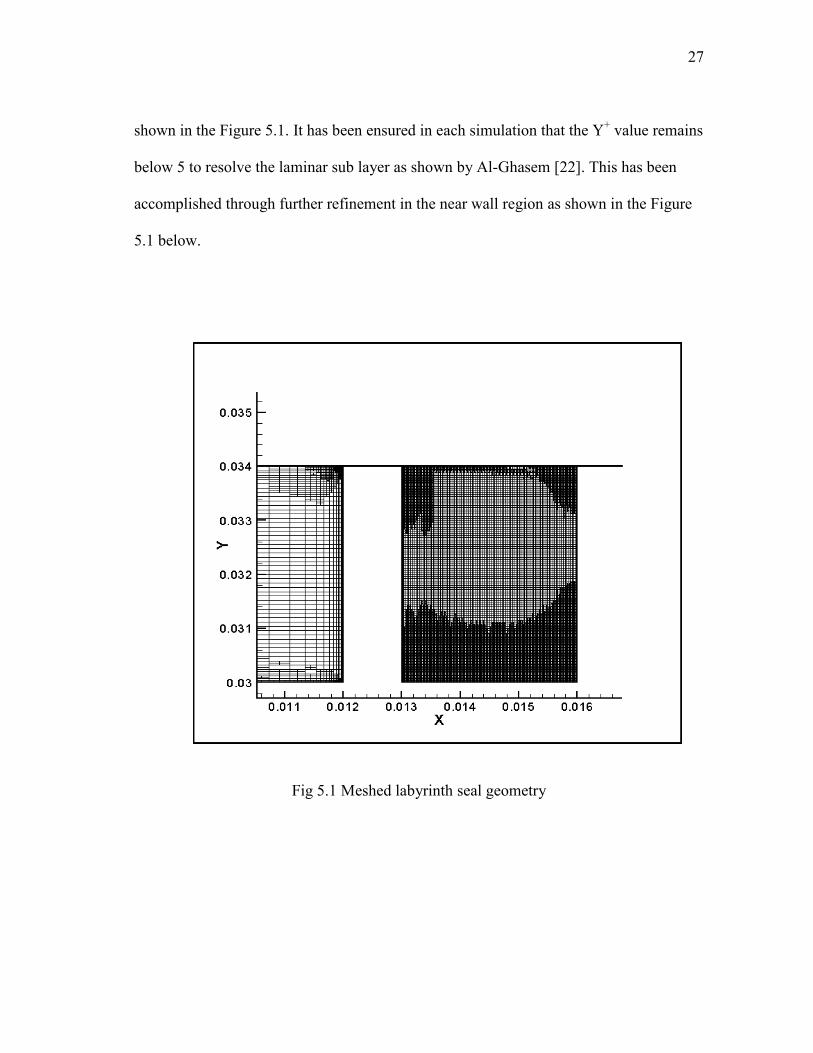
27
shown in the Figure 5.1. It has been ensured in each simulation that the Y+ value remains
below 5 to resolve the laminar sub layer as shown by Al-Ghasem [22]. This has been
accomplished through further refinement in the near wall region as shown in the Figure
5.1 below.
Fig 5.1 Meshed labyrinth seal geometry
28
Regarding the modeling in the near wall region in conjugation with k-ε model
(which has been developed for free turbulence) a separate model needs to be defined.
The standard wall function does not sufficiently resolve the viscous sub-layer, and is not
very effective when the wall is moving rapidly or when there are high pressure gradient
effects. Ideally the wall Y+ values should be below 1. Furthermore it has been suggested
by Morrison-Al Ghasem [22] to use enhanced wall treatment in conjugation with
standard k-ε model to accurately simulate the boundary layer flow with pressure
gradients into consideration. The enhanced wall treatment is necessary to capture flow
characteristics accurately in the viscous sub-layer next to the wall with lesser grid nodes.
For this model Fluent allows wall y+ values as large as 5 given the first layer of the
mesh lie in the viscous sub-layer.
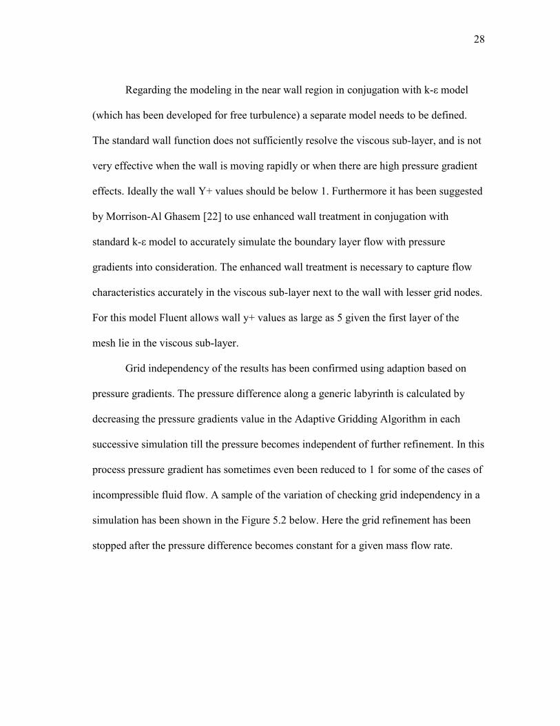
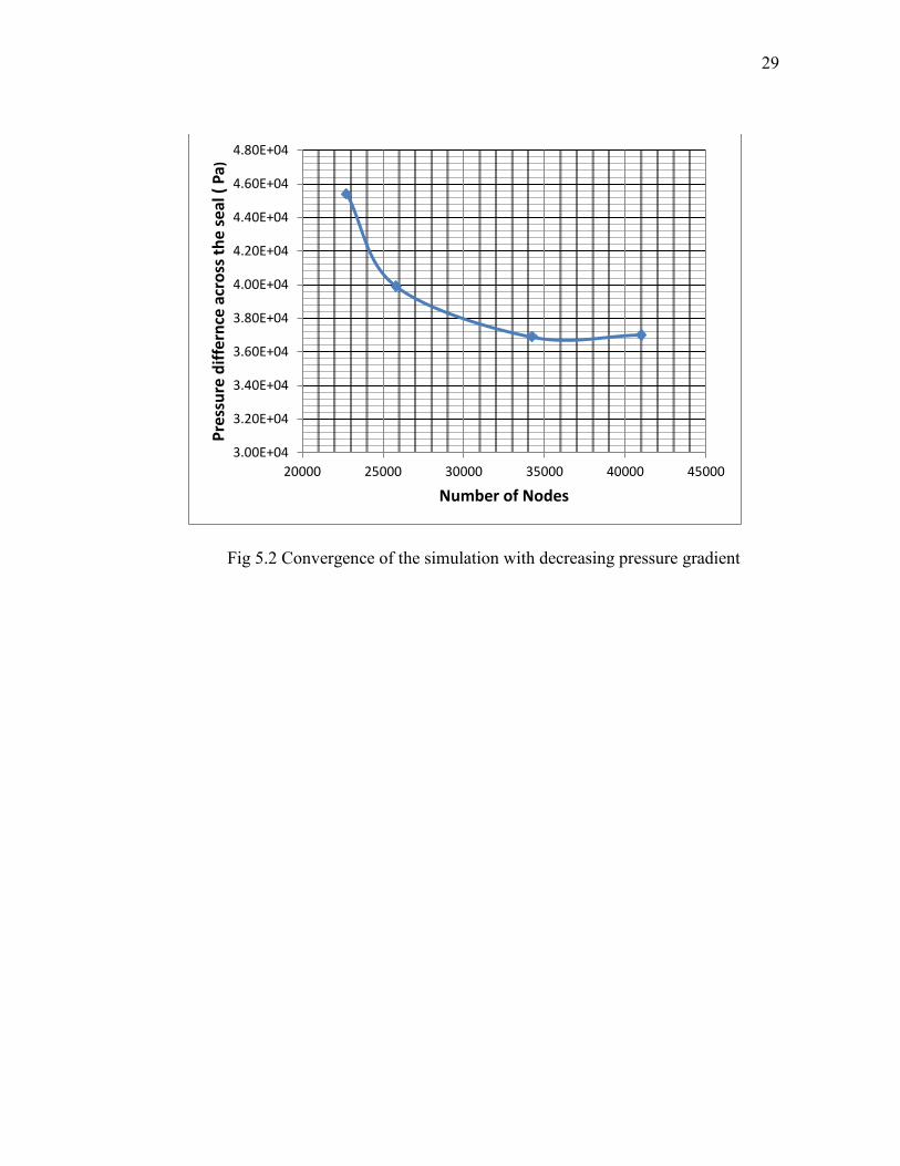
Grid independency of the results has been confirmed using adaption based on
pressure gradients. The pressure difference along a generic labyrinth is calculated by
decreasing the pressure gradients value in the Adaptive Gridding Algorithm in each
successive simulation till the pressure becomes independent of further refinement. In this
process pressure gradient has sometimes even been reduced to 1 for some of the cases of
incompressible fluid flow. A sample of the variation of checking grid independency in a
simulation has been shown in the Figure 5.2 below. Here the grid refinement has been
stopped after the pressure difference becomes constant for a given mass flow rate.
29
Fig 5.2 Convergence of the simulation with decreasing pressure gradient
3.00E+04
3.20E+04
3.40E+04
3.60E+04
3.80E+04
4.00E+04
4.20E+04
4.40E+04
4.60E+04
4.80E+04
20000 25000 30000 35000 40000 45000
Pre
ssu
re d
iffe
rnce
acr
oss
th
e se
al (
Pa
)
Number of Nodes
30
6. CARRY OVER COEFFICIENT
6.1 Introduction
The carry over coefficient is used to measure the effectiveness of the cavity in
terms of flow losses. This factor is used to measure how much of the actual amount of
the kinetic energy before the start of the cavity is actually dissipated through turbulence
dissipation. The lower the carry over coefficient is the more effective is the seal. Ideally
the desired value of the coefficient is one but it cannot be achieved due to the presence
of the energy spectrum in of turbulent flow field. More details about this can be studied
in a book on turbulent flow. The current work uses the definition proposed by
Hodkinson [3] to calculate the carry over coefficient. The relationships provided are as
mentioned below:
( )
The angle beta (β) is used to define the mean streamline separating the
recirculation zone from the fluid that passes over directly to the next clearance. In other
words, this streamline is virtually acting as mass and energy transfer boundary between
the recirculation zone and the mean flow field. This angle is calculated in the study using
the post processing software Tec plot 360®. The required point is found by examining
the point of zero velocity inside the cavity on the downstream tooth. However, in cases
where the Taylor number to Reynolds number ratio is large, it is relatively hard the find
31
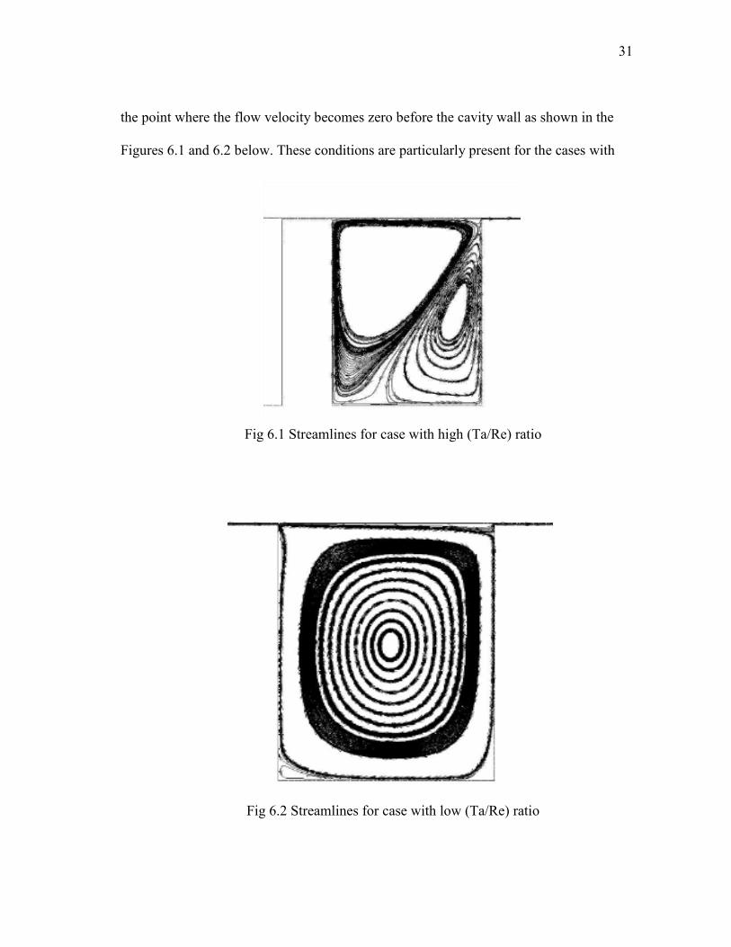
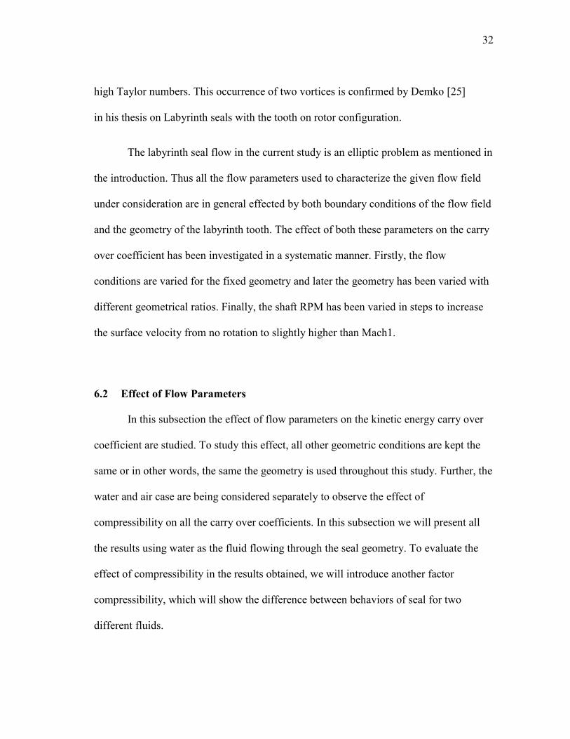
the point where the flow velocity becomes zero before the cavity wall as shown in the
Figures 6.1 and 6.2 below. These conditions are particularly present for the cases with
Fig 6.1 Streamlines for case with high (Ta/Re) ratio
Fig 6.2 Streamlines for case with low (Ta/Re) ratio
32
high Taylor numbers. This occurrence of two vortices is confirmed by Demko [25]
in his thesis on Labyrinth seals with the tooth on rotor configuration.
The labyrinth seal flow in the current study is an elliptic problem as mentioned in
the introduction. Thus all the flow parameters used to characterize the given flow field
under consideration are in general effected by both boundary conditions of the flow field
and the geometry of the labyrinth tooth. The effect of both these parameters on the carry
over coefficient has been investigated in a systematic manner. Firstly, the flow
conditions are varied for the fixed geometry and later the geometry has been varied with
different geometrical ratios. Finally, the shaft RPM has been varied in steps to increase
the surface velocity from no rotation to slightly higher than Mach1.
6.2 Effect of Flow Parameters
In this subsection the effect of flow parameters on the kinetic energy carry over
coefficient are studied. To study this effect, all other geometric conditions are kept the
same or in other words, the same the geometry is used throughout this study. Further, the
water and air case are being considered separately to observe the effect of
compressibility on all the carry over coefficients. In this subsection we will present all
the results using water as the fluid flowing through the seal geometry. To evaluate the
effect of compressibility in the results obtained, we will introduce another factor
compressibility, which will show the difference between behaviors of seal for two
different fluids.
33
6.2.1 Reynolds Number Variation Effect on the Carry over Coefficient
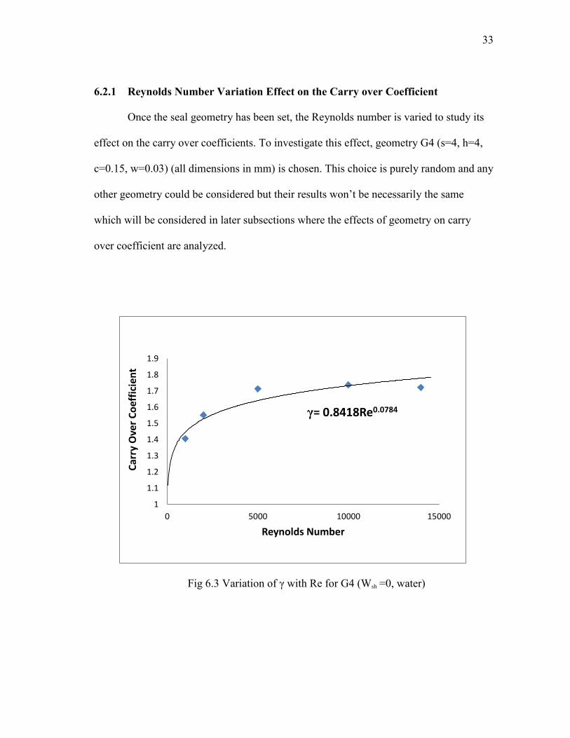
Once the seal geometry has been set, the Reynolds number is varied to study its
effect on the carry over coefficients. To investigate this effect, geometry G4 (s=4, h=4,
c=0.15, w=0.03) (all dimensions in mm) is chosen. This choice is purely random and any
other geometry could be considered but their results won‟t be necessarily the same
which will be considered in later subsections where the effects of geometry on carry
over coefficient are analyzed.
Fig 6.3 Variation of γ with Re for G4 (Wsh =0, water)
γ= 0.8418Re0.0784
1
1.1
1.2
1.3
1.4
1.5
1.6
1.7
1.8
1.9
0 5000 10000 15000
Car
ry O
ver
Co
effi
cien
t
Reynolds Number
34
From the Figure 6.3, it is observed that the variation of the carry over coefficient
varies with the value of Reynolds number. This result confirms that the carry over
coefficient is a function of Reynolds Number (which was neglected in many previous
studies on labyrinth seals, including that of Hodkinson [3] and Gamal [20]). Additionally,
this variation seems to be similar to the case of tooth on stator as studied by Saikishan
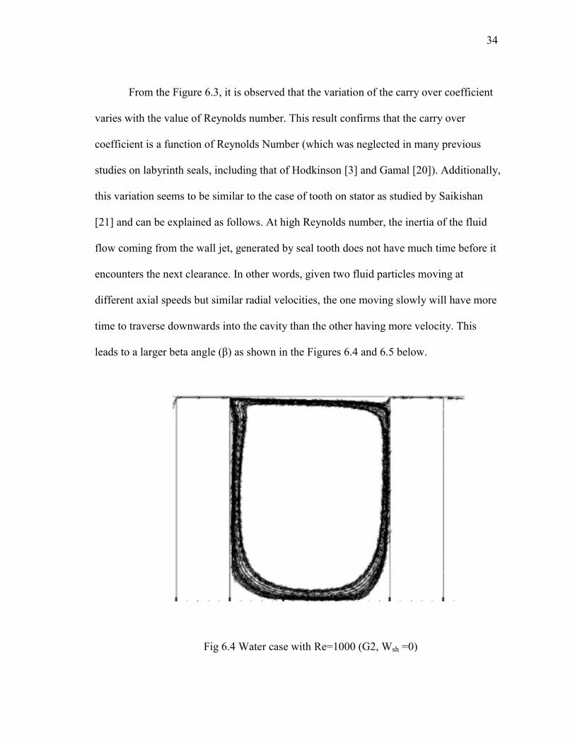
[21] and can be explained as follows. At high Reynolds number, the inertia of the fluid
flow coming from the wall jet, generated by seal tooth does not have much time before it
encounters the next clearance. In other words, given two fluid particles moving at
different axial speeds but similar radial velocities, the one moving slowly will have more
time to traverse downwards into the cavity than the other having more velocity. This
leads to a larger beta angle (β) as shown in the Figures 6.4 and 6.5 below.
Fig 6.4 Water case with Re=1000 (G2, Wsh =0)
35
Fig 6.5 Water case with Re= 2500 (G2, Wsh =0)
The results are quite obvious since this case has been presented for zero shaft
speed. Moreover, a sharp variation in the carry over coefficient as the Reynolds number
increases from 1000 to 2000 is observed and after that the changes become more gradual
because of the change of fluid flow field with increasing Reynolds number is lesser
where other factors also comes into consideration. This shows that the there is a need to
study the effect of changing other parameters such as the shaft speed once a geometry
and Reynolds Number has been fixed upon.
36
6.3 Effect of Geometrical Parameters on the Carry over Coefficient
6.3.1 Effect of Clearance on Carry over Coefficient
From the literature review it has been established that clearance has a major
effect on the labyrinth seal leakage. Since Hodkinson [3], Saikishan [21] and Gamal [20]
had used the non- dimensional form of this clearance as c/s to analyze its effect, the
same parameter will be used in the current research work Furthermore, this non-
dimensional parameter makes it easier to compare and evaluate the results. In this study,
we will compare different seals with the same pitch but different clearances.
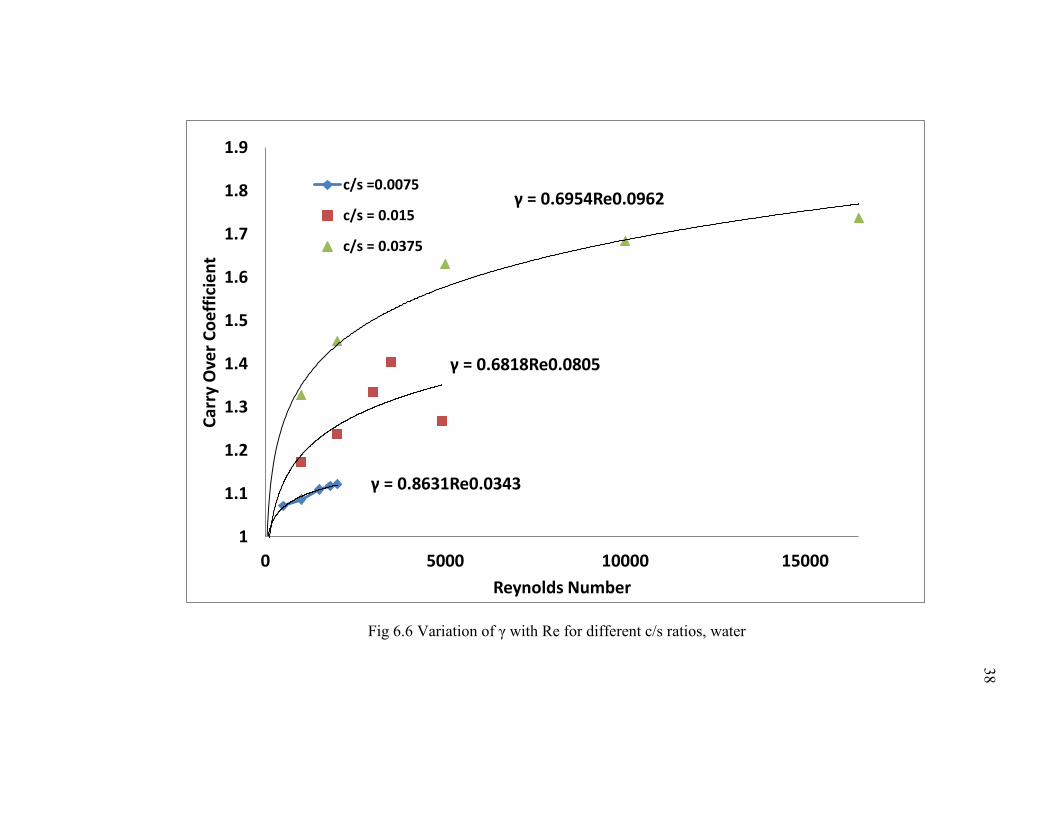
The results of the comparison can be seen in the Figure 6.6. A power law has
been generated in the Figure 6.6 for each set of the different clearance to pitch ratios.
From the Figure 6.6 it is can be seen that there is a great jump in the carry over
coefficient with the corresponding changes in the clearances. The carry over coefficient
reduces 1.6 times (from 1.8 to 1.1) by decreasing the clearance to pitch ratio by 80%
(from c/s = 0.0375 to c/s = 0.0075) at a Reynolds number of 16000. Further, this
decrease in carry over coefficient is fully dependent on the Reynolds number as is seen
from graph. The value of γ increases by 21% by increasing the value of clearance by a
factor of 2.5 at the Reynolds number of 15000. The observation of increasing carry over
coefficient with increasing c/s ratio can also be explained from the hypothesis of
Hodkinson [3]. In his theory, Hodkinson [3] has stated “For a given divergence angle a
higher value of pitch results in a higher impingement point of the jet on the downstream
tooth”. This results in a small portion of fluid flowing to the next clearance resulting in
37
decrease of γ. Therefore an increase of c increases γ or in other words increment in c/s
ratio increases the carry over coefficient. Note that as γ increases, the amount of kinetic
energy dissipated in the seal cavity decreases indicating a seal design that is less
effective at reducing leakage. It has to be noted that, in order to make physical
significance the carry over coefficient should approach 1 as Re approaches 0. This has
been further confirmed by the Figure 6.6.
6.3.2 Effect of Tooth Width on the Carry over Coefficient
In the earlier subsections, the variation of the carry over coefficient with the
clearance to pitch ratio and Reynolds Number for incompressible flow was examined.
However, the other geometrical constants including the tooth width had been fixed. This
is not always true in the real applications of the labyrinth seals. Here the effect of this
parameter on the carry over coefficient will be analyzed which will provide a better
insight in the variation of flow field while changing tooth width. The current study
38
Fig 6.6 Variation of γ with Re for different c/s ratios, water
γ = 0.8631Re0.0343
γ = 0.6818Re0.0805
γ = 0.6954Re0.0962
1
1.1
1.2
1.3
1.4
1.5
1.6
1.7
1.8
1.9
0 5000 10000 15000
Car
ry O
ver
Co
effi
cie
nt
Reynolds Number
c/s =0.0075
c/s = 0.015
c/s = 0.0375
39
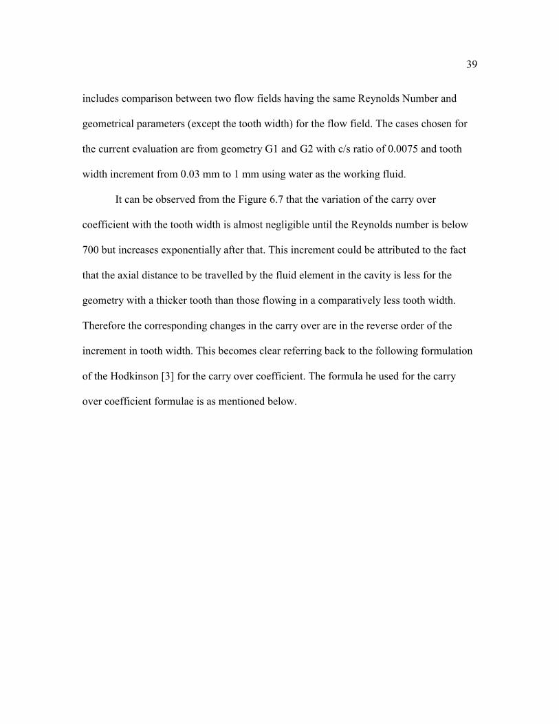
includes comparison between two flow fields having the same Reynolds Number and
geometrical parameters (except the tooth width) for the flow field. The cases chosen for
the current evaluation are from geometry G1 and G2 with c/s ratio of 0.0075 and tooth
width increment from 0.03 mm to 1 mm using water as the working fluid.
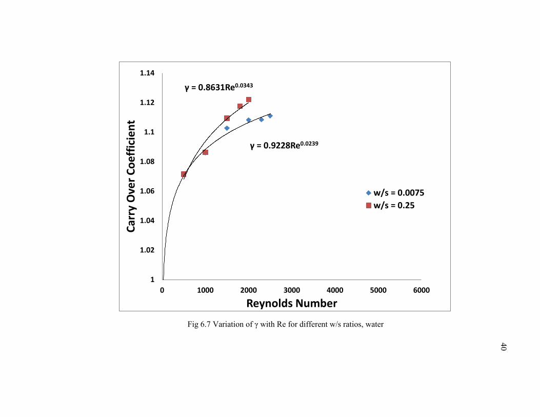
It can be observed from the Figure 6.7 that the variation of the carry over
coefficient with the tooth width is almost negligible until the Reynolds number is below
700 but increases exponentially after that. This increment could be attributed to the fact
that the axial distance to be travelled by the fluid element in the cavity is less for the
geometry with a thicker tooth than those flowing in a comparatively less tooth width.
Therefore the corresponding changes in the carry over are in the reverse order of the
increment in tooth width. This becomes clear referring back to the following formulation
of the Hodkinson [3] for the carry over coefficient. The formula he used for the carry
over coefficient formulae is as mentioned below.
40
Fig 6.7 Variation of γ with Re for different w/s ratios, water
γ = 0.9228Re0.0239
γ = 0.8631Re0.0343
1
1.02
1.04
1.06
1.08
1.1
1.12
1.14
0 1000 2000 3000 4000 5000 6000
Car
ry O
ver
Co
eff
icie
nt
Reynolds Number
w/s = 0.0075
w/s = 0.25
41
√( ( ) (
)
( ) ( )
)
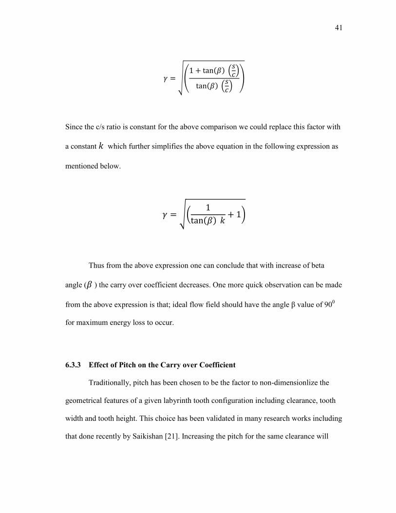
Since the c/s ratio is constant for the above comparison we could replace this factor with
a constant which further simplifies the above equation in the following expression as
mentioned below.
√(
( ) )
Thus from the above expression one can conclude that with increase of beta
angle ( ) the carry over coefficient decreases. One more quick observation can be made
from the above expression is that; ideal flow field should have the angle β value of 900
for maximum energy loss to occur.
6.3.3 Effect of Pitch on the Carry over Coefficient
Traditionally, pitch has been chosen to be the factor to non-dimensionlize the
geometrical features of a given labyrinth tooth configuration including clearance, tooth
width and tooth height. This choice has been validated in many research works including
that done recently by Saikishan [21]. Increasing the pitch for the same clearance will
42
decrease the carry over coefficient. This result should be opposite for increasing of
clearance with fixed pitch. Also this change should be more prominent at high Reynolds
numbers. The same effect is expected to be observed with the tooth width. The carry
over coefficient value should decrease with the increase in the tooth width and this effect
should also be more prominent with higher Reynolds number.
6.3.4 Effect of Shaft Speed Variation on Carry over Coefficient
Completing the analysis of observing the effect of flow parameters (i.e. Reynolds
Number) and geometrical parameters (non-dimensional) parameters on carry over
coefficient we study variation of carry over coefficient with changing speed of rotating
boundary condition.
The rotation of shaft creates an additional introduction of swirl velocity. This
makes it important to study effect of shaft speed on carry over coefficient. The effect of
swirl velocity on the instability of the flow field is also defined by Taylor Number. To
compare the effects of shaft speed, the forces involved in the variation of carry over
coefficient must be considered.
43
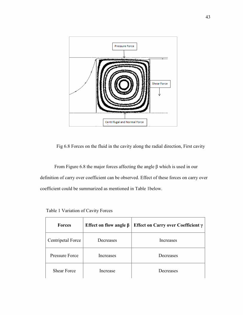
Fig 6.8 Forces on the fluid in the cavity along the radial direction, First cavity
From Figure 6.8 the major forces affecting the angle β which is used in our
definition of carry over coefficient can be observed. Effect of these forces on carry over
coefficient could be summarized as mentioned in Table 1below.
Table 1 Variation of Cavity Forces
Forces Effect on flow angle β Effect on Carry over Coefficient γ
Centripetal Force Decreases Increases
Pressure Force Increases Decreases
Shear Force Increase Decreases
44
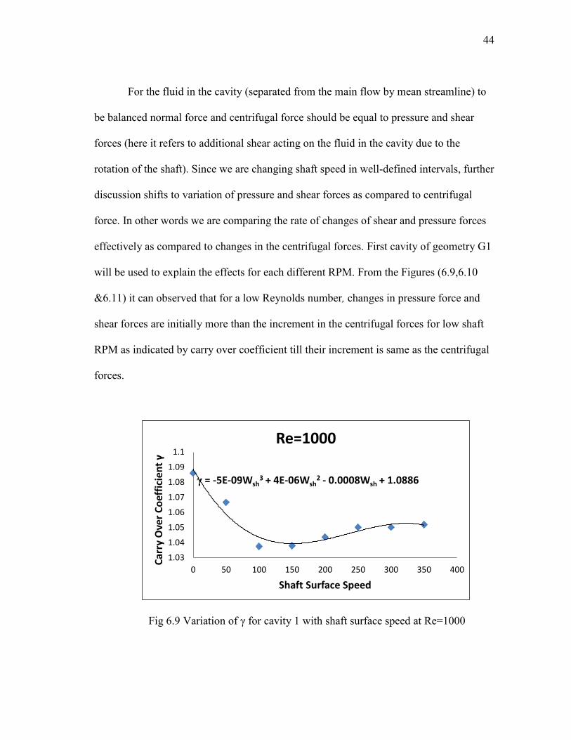
For the fluid in the cavity (separated from the main flow by mean streamline) to
be balanced normal force and centrifugal force should be equal to pressure and shear
forces (here it refers to additional shear acting on the fluid in the cavity due to the
rotation of the shaft). Since we are changing shaft speed in well-defined intervals, further
discussion shifts to variation of pressure and shear forces as compared to centrifugal
force. In other words we are comparing the rate of changes of shear and pressure forces
effectively as compared to changes in the centrifugal forces. First cavity of geometry G1
will be used to explain the effects for each different RPM. From the Figures (6.9,6.10
&6.11) it can observed that for a low Reynolds number, changes in pressure force and
shear forces are initially more than the increment in the centrifugal forces for low shaft
RPM as indicated by carry over coefficient till their increment is same as the centrifugal
forces.
Fig 6.9 Variation of γ for cavity 1 with shaft surface speed at Re=1000
γ = -5E-09Wsh3 + 4E-06Wsh
2 - 0.0008Wsh + 1.0886
1.03
1.04
1.05
1.06
1.07
1.08
1.09
1.1
0 50 100 150 200 250 300 350 400
Car
ry O
ver
Co
effi
cien
t γ
Shaft Surface Speed
Re=1000
45
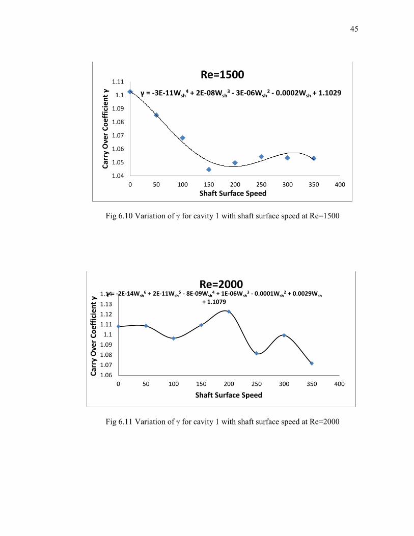
Fig 6.10 Variation of γ for cavity 1 with shaft surface speed at Re=1500
Fig 6.11 Variation of γ for cavity 1 with shaft surface speed at Re=2000
γ = -3E-11Wsh4 + 2E-08Wsh
3 - 3E-06Wsh2 - 0.0002Wsh + 1.1029
1.04
1.05
1.06
1.07
1.08
1.09
1.1
1.11
0 50 100 150 200 250 300 350 400
Car
ry O
ver
Co
effi
cien
t γ
Shaft Surface Speed
Re=1500
γ = -2E-14Wsh6 + 2E-11Wsh
5 - 8E-09Wsh4 + 1E-06Wsh
3 - 0.0001Wsh2 + 0.0029Wsh
+ 1.1079
1.06
1.07
1.08
1.09
1.1
1.11
1.12
1.13
1.14
0 50 100 150 200 250 300 350 400
Car
ry O
ver
Co
effi
cien
t γ
Shaft Surface Speed
Re=2000
46
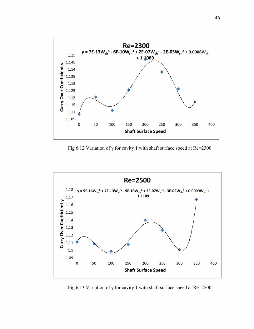
Fig 6.12 Variation of γ for cavity 1 with shaft surface speed at Re=2300
Fig 6.13 Variation of γ for cavity 1 with shaft surface speed at Re=2500
γ = 7E-13Wsh5 - 6E-10Wsh
4 + 2E-07Wsh3 - 2E-05Wsh
2 + 0.0008Wsh + 1.1089
1.105
1.11
1.115
1.12
1.125
1.13
1.135
1.14
1.145
1.15
0 50 100 150 200 250 300 350 400
Car
ry O
ver
Co
effi
cien
t γ
Shaft Surface Speed
Re=2300
γ = 9E-16Wsh6 + 7E-13Wsh
5 - 9E-10Wsh4 + 3E-07Wsh
3 - 3E-05Wsh2 + 0.0009Wsh +
1.1109
1.09
1.1
1.11
1.12
1.13
1.14
1.15
1.16
1.17
1.18
0 50 100 150 200 250 300 350 400
Car
ry O
ver
Co
effi
cien
t γ
Shaft Surface Speed
Re=2500
47
Same is observed for Figures (6.12 & 6.13) This trend is observed in both the
case with Re=1000 & Re=1500. For Re=2000 the increment is same till the shaft surface
speed reaches 50 m/s. After that the increment in pressure force and shear forces is less
than in centrifugal forces and this continues till shaft surface speed reaches 200m/s
above which it becomes same as for low Re.
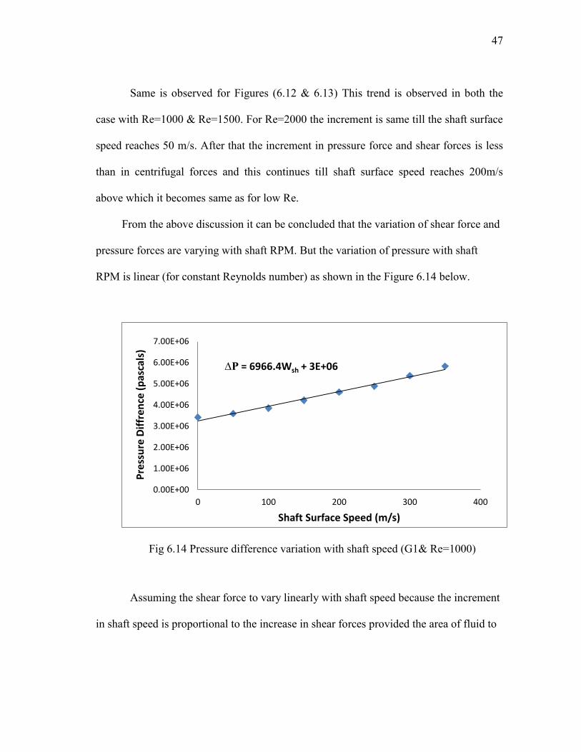
From the above discussion it can be concluded that the variation of shear force and
pressure forces are varying with shaft RPM. But the variation of pressure with shaft
RPM is linear (for constant Reynolds number) as shown in the Figure 6.14 below.
Fig 6.14 Pressure difference variation with shaft speed (G1& Re=1000)
Assuming the shear force to vary linearly with shaft speed because the increment
in shaft speed is proportional to the increase in shear forces provided the area of fluid to
∆P = 6966.4Wsh + 3E+06
0.00E+00
1.00E+06
2.00E+06
3.00E+06
4.00E+06
5.00E+06
6.00E+06
7.00E+06
0 100 200 300 400
Pre
ssu
re D
iffr
ence
(p
asca
ls)
Shaft Surface Speed (m/s)
48
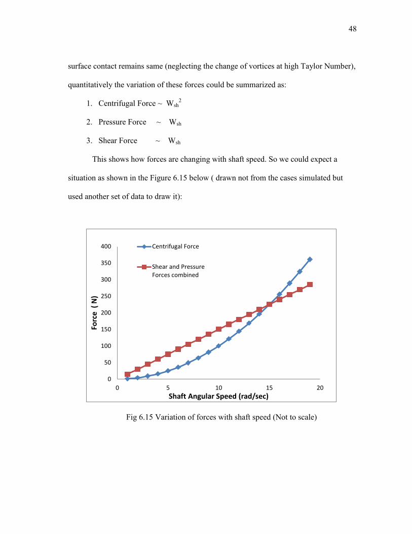
surface contact remains same (neglecting the change of vortices at high Taylor Number),
quantitatively the variation of these forces could be summarized as:
1. Centrifugal Force ~ Wsh2
2. Pressure Force ~ Wsh
3. Shear Force ~ Wsh
This shows how forces are changing with shaft speed. So we could expect a
situation as shown in the Figure 6.15 below ( drawn not from the cases simulated but
used another set of data to draw it):
Fig 6.15 Variation of forces with shaft speed (Not to scale)
0
50
100
150
200
250
300
350
400
0 5 10 15 20
Forc
e (
N)
Shaft Angular Speed (rad/sec)
Centrifugal Force
Shear and PressureForces combined
49
From here, understanding of the variation of carry over coefficient for different cases is
achieved. It may be explained as, for different Reynolds number the slope of the
pressure force and shear force will be different from centrifugal forces which change the
crossing points of two graphs. Also if we further consider the variation of vortex
formation in cavity at high Taylor Number there can be more variation in this graph by
changing the slope of straight line at different shaft speed. This will lead to more points
of intersections which correspond to ups and downs in the carry over coefficient graph
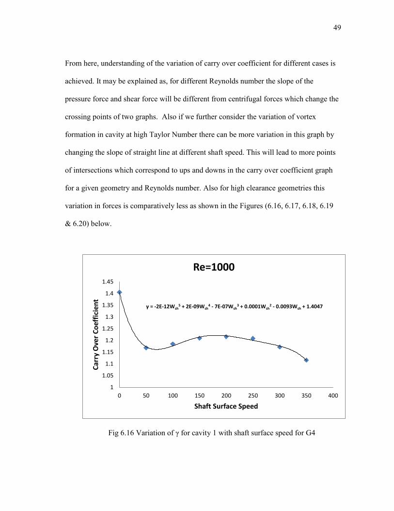
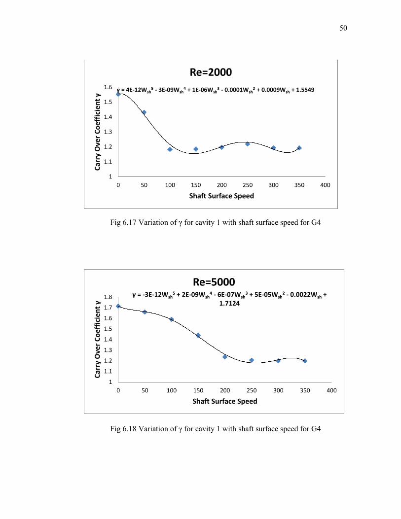
for a given geometry and Reynolds number. Also for high clearance geometries this
variation in forces is comparatively less as shown in the Figures (6.16, 6.17, 6.18, 6.19
& 6.20) below.
Fig 6.16 Variation of γ for cavity 1 with shaft surface speed for G4
γ = -2E-12Wsh5 + 2E-09Wsh
4 - 7E-07Wsh3 + 0.0001Wsh
2 - 0.0093Wsh + 1.4047
1
1.05
1.1
1.15
1.2
1.25
1.3
1.35
1.4
1.45
0 50 100 150 200 250 300 350 400
Car
ry O
ver
Co
effi
cien
t
Shaft Surface Speed
Re=1000
50
Fig 6.17 Variation of γ for cavity 1 with shaft surface speed for G4
Fig 6.18 Variation of γ for cavity 1 with shaft surface speed for G4
γ = 4E-12Wsh5 - 3E-09Wsh
4 + 1E-06Wsh3 - 0.0001Wsh
2 + 0.0009Wsh + 1.5549
1
1.1
1.2
1.3
1.4
1.5
1.6
0 50 100 150 200 250 300 350 400
Car
ry O
ver
Co
effi
cien
t γ
Shaft Surface Speed
Re=2000
γ = -3E-12Wsh5 + 2E-09Wsh
4 - 6E-07Wsh3 + 5E-05Wsh
2 - 0.0022Wsh + 1.7124
1
1.1
1.2
1.3
1.4
1.5
1.6
1.7
1.8
0 50 100 150 200 250 300 350 400
Car
ry O
ver
Co
effi
cien
t γ
Shaft Surface Speed
Re=5000
51
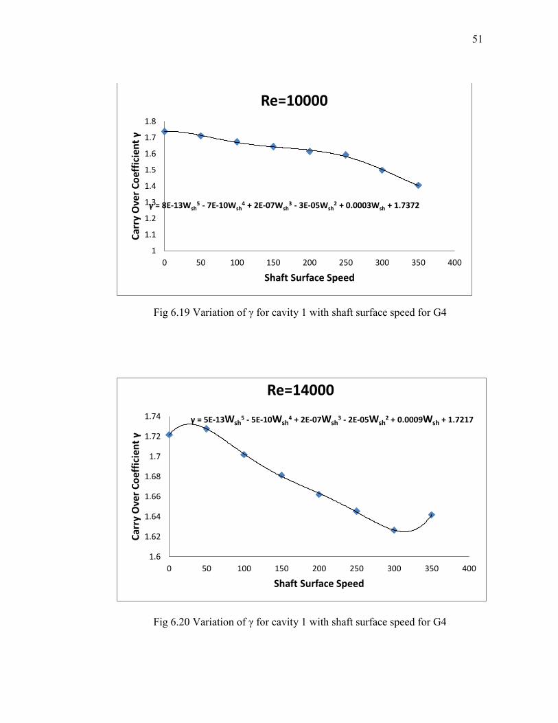
Fig 6.19 Variation of γ for cavity 1 with shaft surface speed for G4
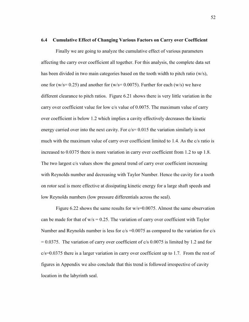
Fig 6.20 Variation of γ for cavity 1 with shaft surface speed for G4
γ = 8E-13Wsh5 - 7E-10Wsh
4 + 2E-07Wsh3 - 3E-05Wsh
2 + 0.0003Wsh + 1.7372
1
1.1
1.2
1.3
1.4
1.5
1.6
1.7
1.8
0 50 100 150 200 250 300 350 400
Car
ry O
ver
Co
effi
cien
t γ
Shaft Surface Speed
Re=10000
γ = 5E-13Wsh5 - 5E-10Wsh
4 + 2E-07Wsh3 - 2E-05Wsh
2 + 0.0009Wsh + 1.7217
1.6
1.62
1.64
1.66
1.68
1.7
1.72
1.74
0 50 100 150 200 250 300 350 400
Car
ry O
ver
Co
effi
cien
t γ
Shaft Surface Speed
Re=14000
52
6.4 Cumulative Effect of Changing Various Factors on Carry over Coefficient
Finally we are going to analyze the cumulative effect of various parameters
affecting the carry over coefficient all together. For this analysis, the complete data set
has been divided in two main categories based on the tooth width to pitch ratio (w/s),
one for (w/s= 0.25) and another for (w/s= 0.0075). Further for each (w/s) we have
different clearance to pitch ratios. Figure 6.21 shows there is very little variation in the
carry over coefficient value for low c/s value of 0.0075. The maximum value of carry
over coefficient is below 1.2 which implies a cavity effectively decreases the kinetic
energy carried over into the next cavity. For c/s= 0.015 the variation similarly is not
much with the maximum value of carry over coefficient limited to 1.4. As the c/s ratio is
increased to 0.0375 there is more variation in carry over coefficient from 1.2 to up 1.8.
The two largest c/s values show the general trend of carry over coefficient increasing
with Reynolds number and decreasing with Taylor Number. Hence the cavity for a tooth
on rotor seal is more effective at dissipating kinetic energy for a large shaft speeds and
low Reynolds numbers (low pressure differentials across the seal).
Figure 6.22 shows the same results for w/s=0.0075. Almost the same observation
can be made for that of w/s = 0.25. The variation of carry over coefficient with Taylor
Number and Reynolds number is less for c/s =0.0075 as compared to the variation for c/s
= 0.0375. The variation of carry over coefficient of c/s 0.0075 is limited by 1.2 and for
c/s=0.0375 there is a larger variation in carry over coefficient up to 1.7. From the rest of
figures in Appendix we also conclude that this trend is followed irrespective of cavity
location in the labyrinth seal.
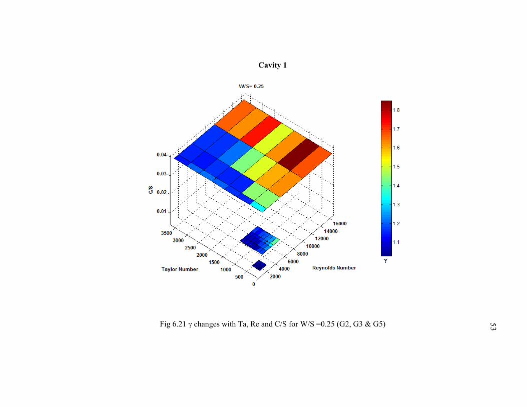
53
Cavity 1
Fig 6.21 γ changes with Ta, Re and C/S for W/S =0.25 (G2, G3 & G5)
53
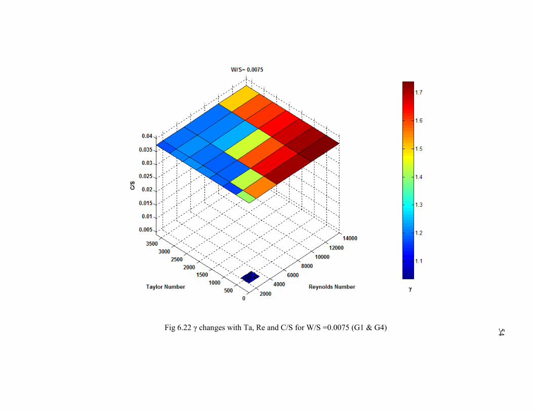
54
Fig 6.22 γ changes with Ta, Re and C/S for W/S =0.0075 (G1 & G4) 54
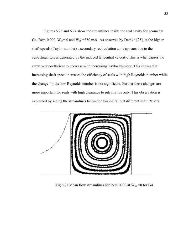
55
Figures 6.23 and 6.24 show the streamlines inside the seal cavity for geometry
G4, Re=10,000, Wsh= 0 and Wsh =350 m/s. As observed by Demko [25], at the higher
shaft speeds (Taylor number) a secondary recirculation zone appears due to the
centrifugal forces generated by the induced tangential velocity. This is what causes the
carry over coefficient to decrease with increasing Taylor Number. This shows that
increasing shaft speed increases the efficiency of seals with high Reynolds number while
the change for the low Reynolds number is not significant. Further these changes are
more important for seals with high clearance to pitch ratios only. This observation is
explained by seeing the streamlines below for low c/s ratio at different shaft RPM‟s.
Fig 6.23 Mean flow streamlines for Re=10000 at Wsh =0 for G4
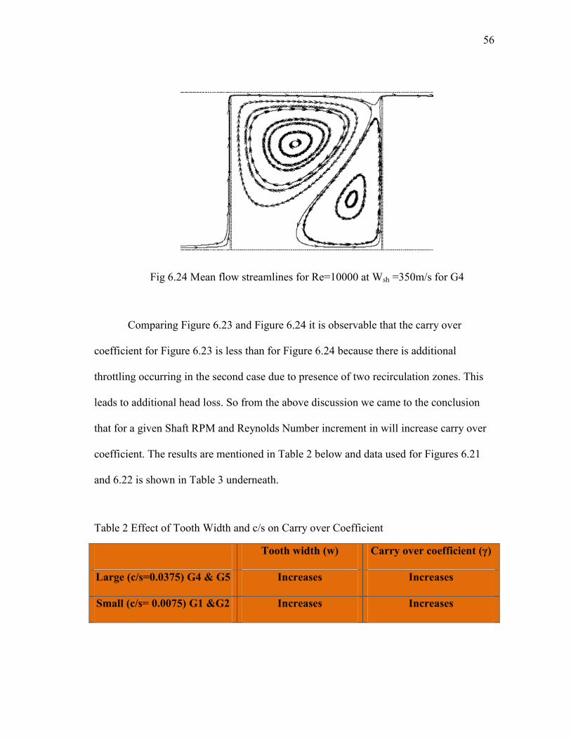
56
Fig 6.24 Mean flow streamlines for Re=10000 at Wsh =350m/s for G4
Comparing Figure 6.23 and Figure 6.24 it is observable that the carry over
coefficient for Figure 6.23 is less than for Figure 6.24 because there is additional
throttling occurring in the second case due to presence of two recirculation zones. This
leads to additional head loss. So from the above discussion we came to the conclusion
that for a given Shaft RPM and Reynolds Number increment in will increase carry over
coefficient. The results are mentioned in Table 2 below and data used for Figures 6.21
and 6.22 is shown in Table 3 underneath.
Table 2 Effect of Tooth Width and c/s on Carry over Coefficient
Tooth width (w) Carry over coefficient (γ)
Large (c/s=0.0375) G4 & G5 Increases Increases
Small (c/s= 0.0075) G1 &G2 Increases Increases
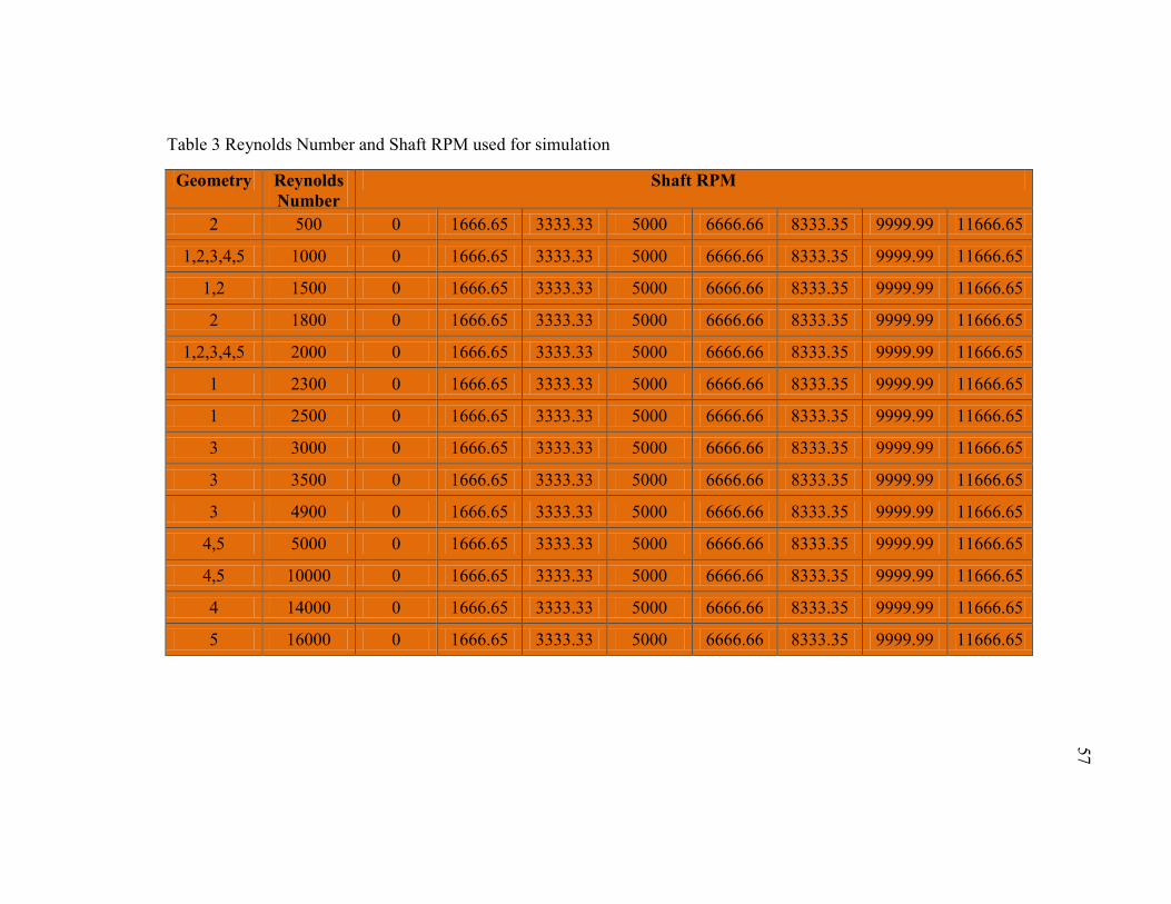
57
Table 3 Reynolds Number and Shaft RPM used for simulation
Geometry Reynolds
Number
Shaft RPM
2 500 0 1666.65 3333.33 5000 6666.66 8333.35 9999.99 11666.65
1,2,3,4,5 1000 0 1666.65 3333.33 5000 6666.66 8333.35 9999.99 11666.65
1,2 1500 0 1666.65 3333.33 5000 6666.66 8333.35 9999.99 11666.65
2 1800 0 1666.65 3333.33 5000 6666.66 8333.35 9999.99 11666.65
1,2,3,4,5 2000 0 1666.65 3333.33 5000 6666.66 8333.35 9999.99 11666.65
1 2300 0 1666.65 3333.33 5000 6666.66 8333.35 9999.99 11666.65
1 2500 0 1666.65 3333.33 5000 6666.66 8333.35 9999.99 11666.65
3 3000 0 1666.65 3333.33 5000 6666.66 8333.35 9999.99 11666.65
3 3500 0 1666.65 3333.33 5000 6666.66 8333.35 9999.99 11666.65
3 4900 0 1666.65 3333.33 5000 6666.66 8333.35 9999.99 11666.65
4,5 5000 0 1666.65 3333.33 5000 6666.66 8333.35 9999.99 11666.65
4,5 10000 0 1666.65 3333.33 5000 6666.66 8333.35 9999.99 11666.65
4 14000 0 1666.65 3333.33 5000 6666.66 8333.35 9999.99 11666.65
5 16000 0 1666.65 3333.33 5000 6666.66 8333.35 9999.99 11666.65
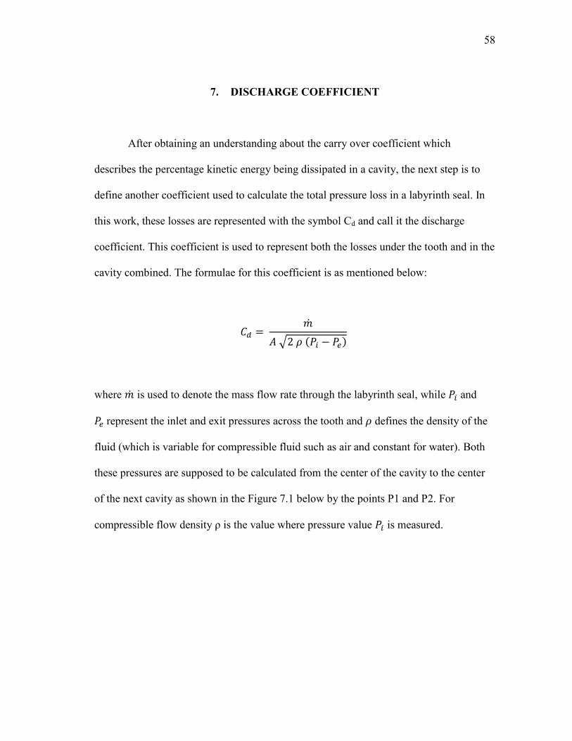
58
7. DISCHARGE COEFFICIENT
After obtaining an understanding about the carry over coefficient which
describes the percentage kinetic energy being dissipated in a cavity, the next step is to
define another coefficient used to calculate the total pressure loss in a labyrinth seal. In
this work, these losses are represented with the symbol Cd and call it the discharge
coefficient. This coefficient is used to represent both the losses under the tooth and in the
cavity combined. The formulae for this coefficient is as mentioned below:
√ ( )
where is used to denote the mass flow rate through the labyrinth seal, while and
represent the inlet and exit pressures across the tooth and defines the density of the
fluid (which is variable for compressible fluid such as air and constant for water). Both
these pressures are supposed to be calculated from the center of the cavity to the center
of the next cavity as shown in the Figure 7.1 below by the points P1 and P2. For
compressible flow density is the value where pressure value is measured.
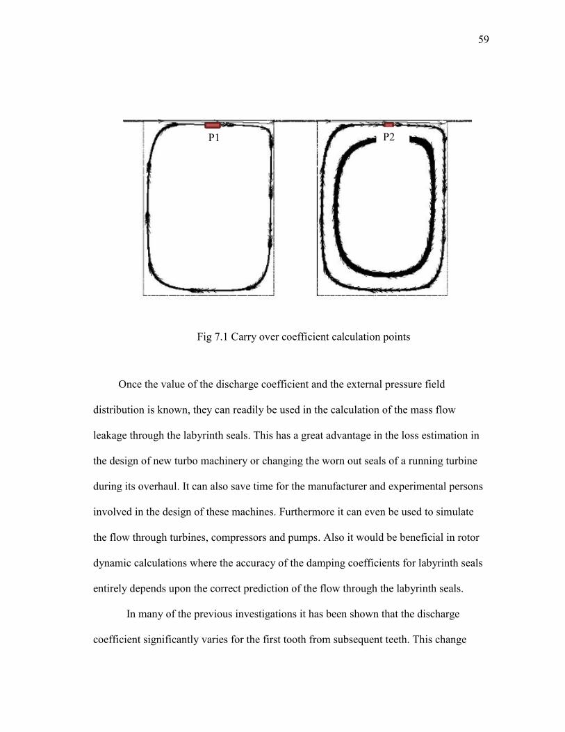
59
Fig 7.1 Carry over coefficient calculation points
Once the value of the discharge coefficient and the external pressure field
distribution is known, they can readily be used in the calculation of the mass flow
leakage through the labyrinth seals. This has a great advantage in the loss estimation in
the design of new turbo machinery or changing the worn out seals of a running turbine
during its overhaul. It can also save time for the manufacturer and experimental persons
involved in the design of these machines. Furthermore it can even be used to simulate
the flow through turbines, compressors and pumps. Also it would be beneficial in rotor
dynamic calculations where the accuracy of the damping coefficients for labyrinth seals
entirely depends upon the correct prediction of the flow through the labyrinth seals.
In many of the previous investigations it has been shown that the discharge
coefficient significantly varies for the first tooth from subsequent teeth. This change
P1 P2
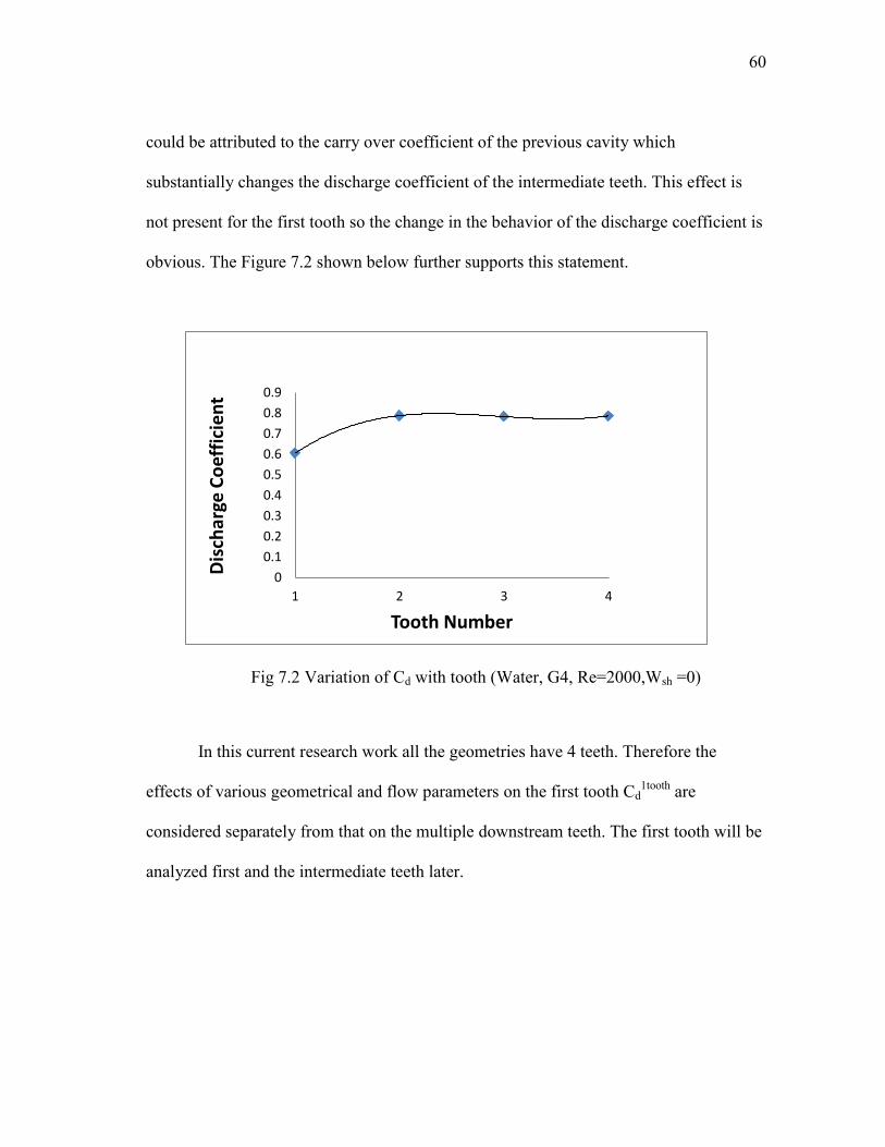
60
could be attributed to the carry over coefficient of the previous cavity which
substantially changes the discharge coefficient of the intermediate teeth. This effect is
not present for the first tooth so the change in the behavior of the discharge coefficient is
obvious. The Figure 7.2 shown below further supports this statement.
Fig 7.2 Variation of Cd with tooth (Water, G4, Re=2000,Wsh =0)
In this current research work all the geometries have 4 teeth. Therefore the
effects of various geometrical and flow parameters on the first tooth Cd1tooth
are
considered separately from that on the multiple downstream teeth. The first tooth will be
analyzed first and the intermediate teeth later.
0
0.1
0.2
0.3
0.4
0.5
0.6
0.7
0.8
0.9
1 2 3 4
Dis
char
ge C
oef
fici
en
t
Tooth Number
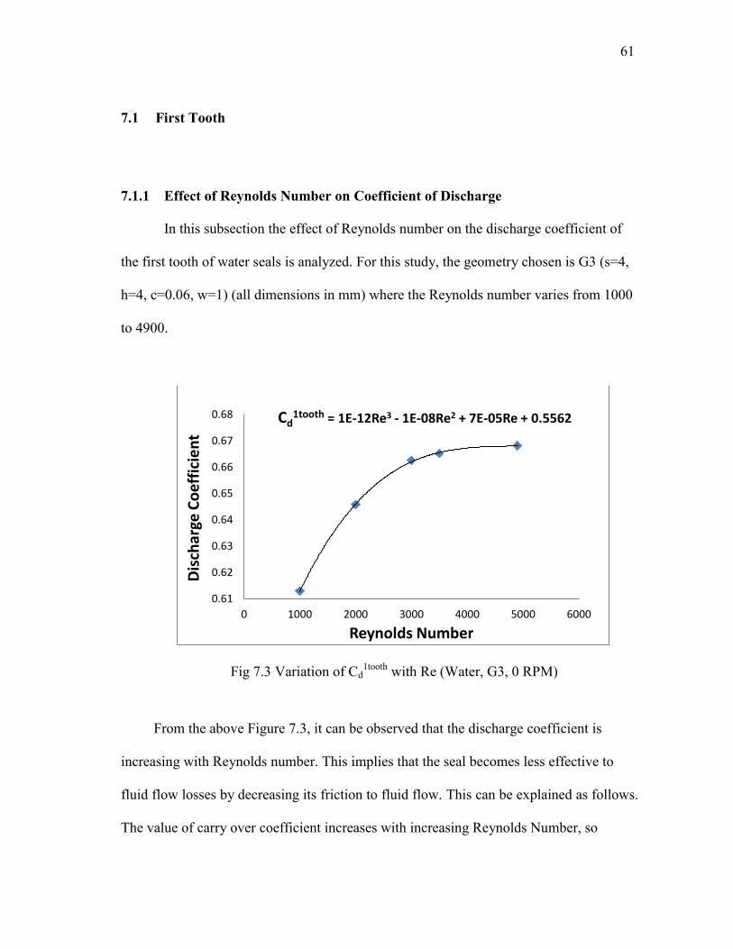
61
7.1 First Tooth
7.1.1 Effect of Reynolds Number on Coefficient of Discharge
In this subsection the effect of Reynolds number on the discharge coefficient of
the first tooth of water seals is analyzed. For this study, the geometry chosen is G3 (s=4,
h=4, c=0.06, w=1) (all dimensions in mm) where the Reynolds number varies from 1000
to 4900.
Fig 7.3 Variation of Cd1tooth
with Re (Water, G3, 0 RPM)
From the above Figure 7.3, it can be observed that the discharge coefficient is
increasing with Reynolds number. This implies that the seal becomes less effective to
fluid flow losses by decreasing its friction to fluid flow. This can be explained as follows.
The value of carry over coefficient increases with increasing Reynolds Number, so
Cd1tooth = 1E-12Re3 - 1E-08Re2 + 7E-05Re + 0.5562
0.61
0.62
0.63
0.64
0.65
0.66
0.67
0.68
0 1000 2000 3000 4000 5000 6000
Dis
char
ge C
oef
fici
en
t
Reynolds Number
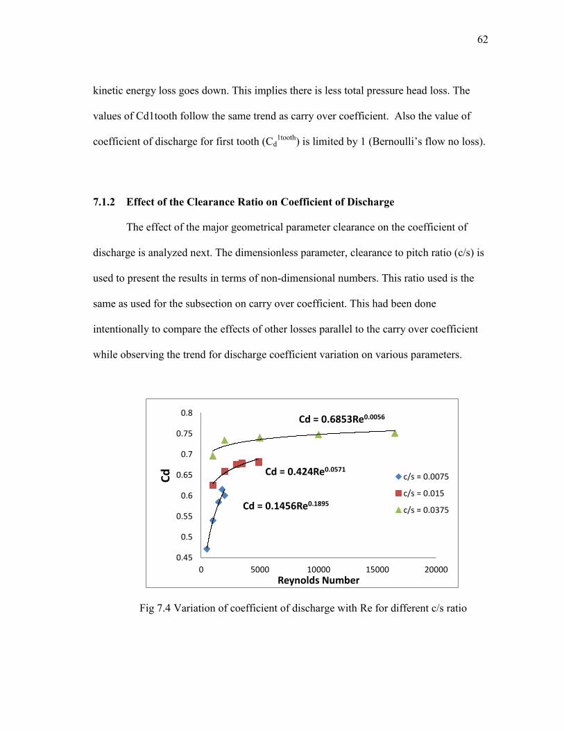
62
kinetic energy loss goes down. This implies there is less total pressure head loss. The
values of Cd1tooth follow the same trend as carry over coefficient. Also the value of
coefficient of discharge for first tooth (Cd1tooth
) is limited by 1 (Bernoulli‟s flow no loss).
7.1.2 Effect of the Clearance Ratio on Coefficient of Discharge
The effect of the major geometrical parameter clearance on the coefficient of
discharge is analyzed next. The dimensionless parameter, clearance to pitch ratio (c/s) is
used to present the results in terms of non-dimensional numbers. This ratio used is the
same as used for the subsection on carry over coefficient. This had been done
intentionally to compare the effects of other losses parallel to the carry over coefficient
while observing the trend for discharge coefficient variation on various parameters.
Fig 7.4 Variation of coefficient of discharge with Re for different c/s ratio
Cd = 0.1456Re0.1895
Cd = 0.424Re0.0571
Cd = 0.6853Re0.0056
0.45
0.5
0.55
0.6
0.65
0.7
0.75
0.8
0 5000 10000 15000 20000
Cd
Reynolds Number
c/s = 0.0075
c/s = 0.015
c/s = 0.0375
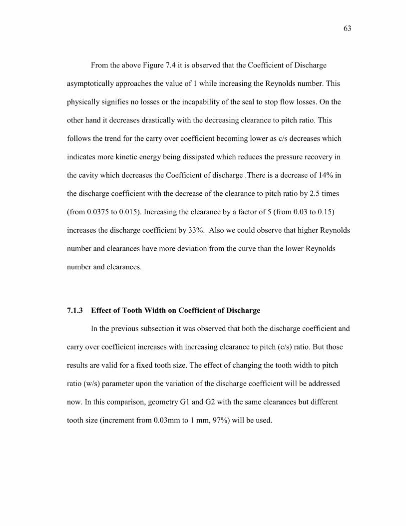
63
From the above Figure 7.4 it is observed that the Coefficient of Discharge
asymptotically approaches the value of 1 while increasing the Reynolds number. This
physically signifies no losses or the incapability of the seal to stop flow losses. On the
other hand it decreases drastically with the decreasing clearance to pitch ratio. This
follows the trend for the carry over coefficient becoming lower as c/s decreases which
indicates more kinetic energy being dissipated which reduces the pressure recovery in
the cavity which decreases the Coefficient of discharge .There is a decrease of 14% in
the discharge coefficient with the decrease of the clearance to pitch ratio by 2.5 times
(from 0.0375 to 0.015). Increasing the clearance by a factor of 5 (from 0.03 to 0.15)
increases the discharge coefficient by 33%. Also we could observe that higher Reynolds
number and clearances have more deviation from the curve than the lower Reynolds
number and clearances.
7.1.3 Effect of Tooth Width on Coefficient of Discharge
In the previous subsection it was observed that both the discharge coefficient and
carry over coefficient increases with increasing clearance to pitch (c/s) ratio. But those
results are valid for a fixed tooth size. The effect of changing the tooth width to pitch
ratio (w/s) parameter upon the variation of the discharge coefficient will be addressed
now. In this comparison, geometry G1 and G2 with the same clearances but different
tooth size (increment from 0.03mm to 1 mm, 97%) will be used.
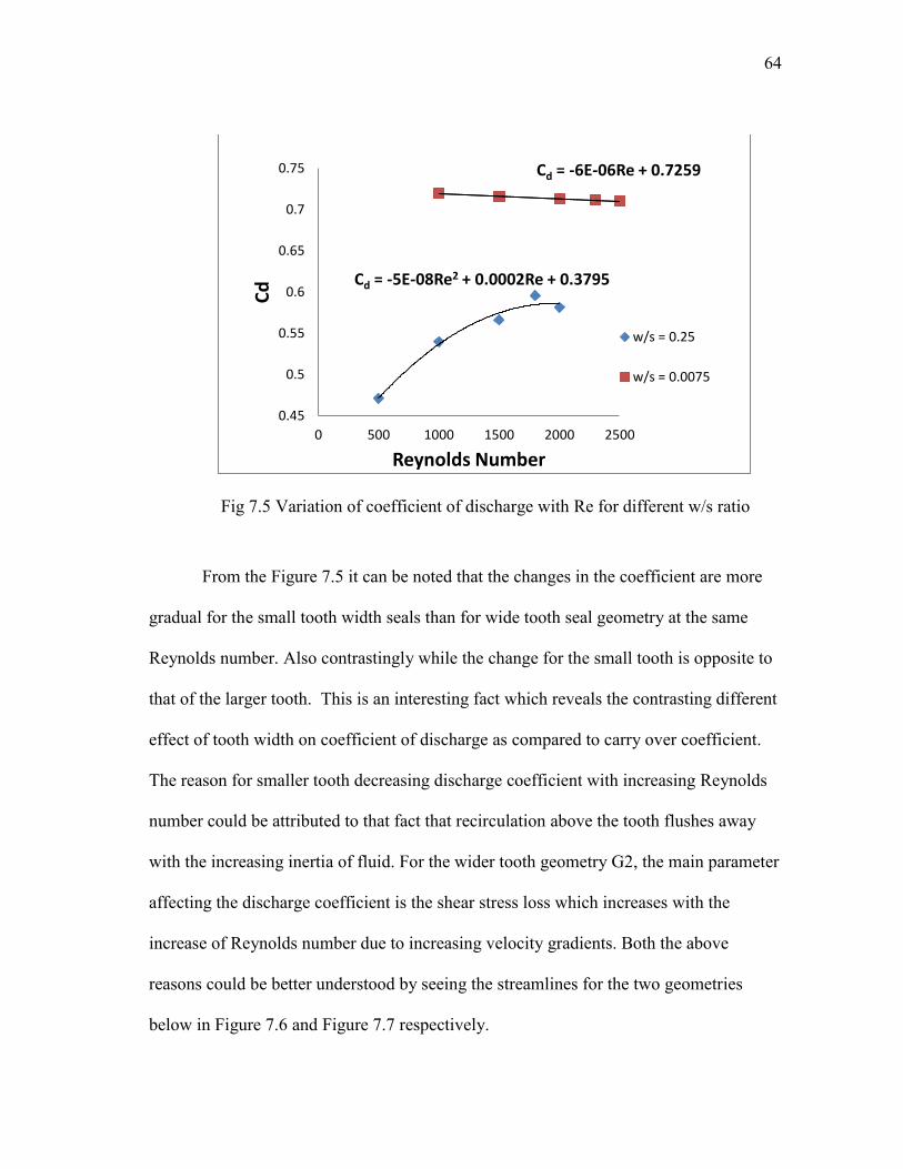
64
Fig 7.5 Variation of coefficient of discharge with Re for different w/s ratio
From the Figure 7.5 it can be noted that the changes in the coefficient are more
gradual for the small tooth width seals than for wide tooth seal geometry at the same
Reynolds number. Also contrastingly while the change for the small tooth is opposite to
that of the larger tooth. This is an interesting fact which reveals the contrasting different
effect of tooth width on coefficient of discharge as compared to carry over coefficient.
The reason for smaller tooth decreasing discharge coefficient with increasing Reynolds
number could be attributed to that fact that recirculation above the tooth flushes away
with the increasing inertia of fluid. For the wider tooth geometry G2, the main parameter
affecting the discharge coefficient is the shear stress loss which increases with the
increase of Reynolds number due to increasing velocity gradients. Both the above
reasons could be better understood by seeing the streamlines for the two geometries
below in Figure 7.6 and Figure 7.7 respectively.
Cd = -5E-08Re2 + 0.0002Re + 0.3795
Cd = -6E-06Re + 0.7259
0.45
0.5
0.55
0.6
0.65
0.7
0.75
0 500 1000 1500 2000 2500
Cd
Reynolds Number
w/s = 0.25
w/s = 0.0075
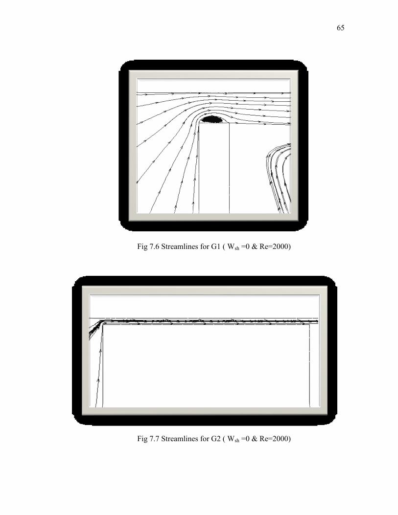
65
Fig 7.6 Streamlines for G1 ( Wsh =0 & Re=2000)
Fig 7.7 Streamlines for G2 ( Wsh =0 & Re=2000)
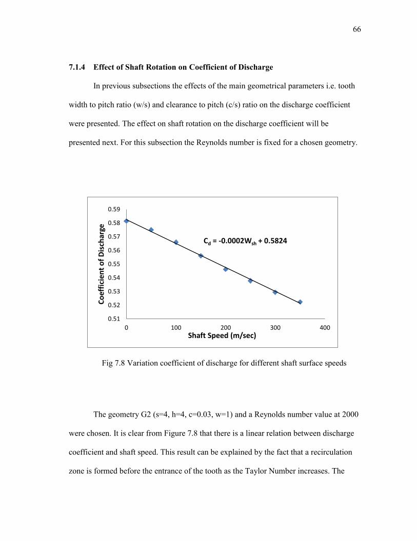
66
7.1.4 Effect of Shaft Rotation on Coefficient of Discharge
In previous subsections the effects of the main geometrical parameters i.e. tooth
width to pitch ratio (w/s) and clearance to pitch (c/s) ratio on the discharge coefficient
were presented. The effect on shaft rotation on the discharge coefficient will be
presented next. For this subsection the Reynolds number is fixed for a chosen geometry.
Fig 7.8 Variation coefficient of discharge for different shaft surface speeds
The geometry G2 (s=4, h=4, c=0.03, w=1) and a Reynolds number value at 2000
were chosen. It is clear from Figure 7.8 that there is a linear relation between discharge
coefficient and shaft speed. This result can be explained by the fact that a recirculation
zone is formed before the entrance of the tooth as the Taylor Number increases. The
Cd = -0.0002Wsh + 0.5824
0.51
0.52
0.53
0.54
0.55
0.56
0.57
0.58
0.59
0 100 200 300 400
Co
effi
cien
t o
f D
isch
arge
Shaft Speed (m/sec)
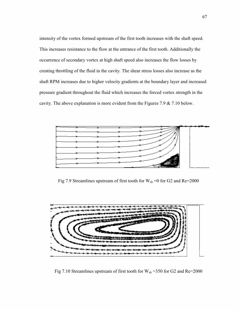
67
intensity of the vortex formed upstream of the first tooth increases with the shaft speed.
This increases resistance to the flow at the entrance of the first tooth. Additionally the
occurrence of secondary vortex at high shaft speed also increases the flow losses by
creating throttling of the fluid in the cavity. The shear stress losses also increase as the
shaft RPM increases due to higher velocity gradients at the boundary layer and increased
pressure gradient throughout the fluid which increases the forced vortex strength in the
cavity. The above explanation is more evident from the Figures 7.9 & 7.10 below.
Fig 7.9 Streamlines upstream of first tooth for Wsh =0 for G2 and Re=2000
Fig 7.10 Streamlines upstream of first tooth for Wsh =350 for G2 and Re=2000
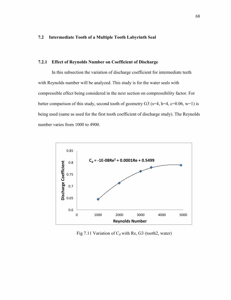
68
7.2 Intermediate Tooth of a Multiple Tooth Labyrinth Seal
7.2.1 Effect of Reynolds Number on Coefficient of Discharge
In this subsection the variation of discharge coefficient for intermediate teeth
with Reynolds number will be analyzed. This study is for the water seals with
compressible effect being considered in the next section on compressibility factor. For
better comparison of this study, second tooth of geometry G3 (s=4, h=4, c=0.06, w=1) is
being used (same as used for the first tooth coefficient of discharge study). The Reynolds
number varies from 1000 to 4900.
Fig 7.11 Variation of Cd with Re, G3 (tooth2, water)
Cd = -1E-08Re2 + 0.0001Re + 0.5499
0.6
0.65
0.7
0.75
0.8
0.85
0 1000 2000 3000 4000 5000
Dis
char
ge C
oef
fici
ent
Reynolds Number
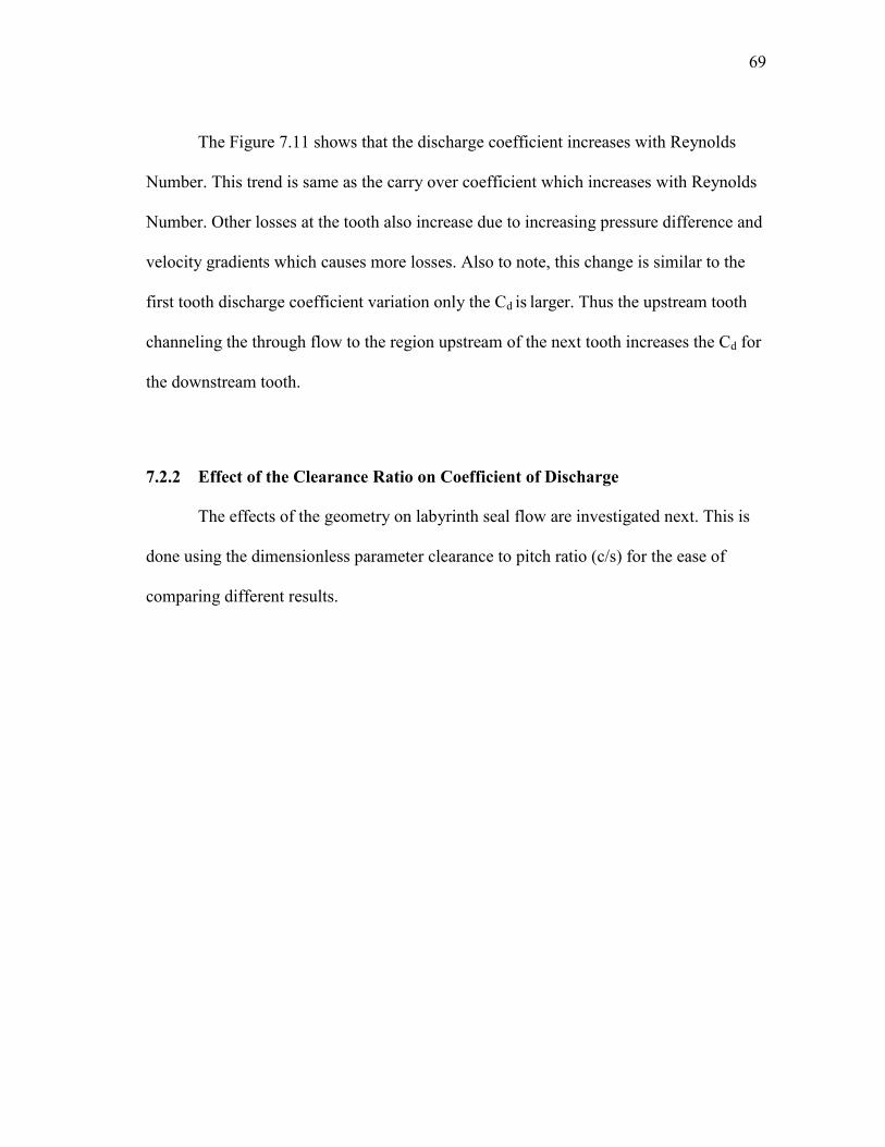
69
The Figure 7.11 shows that the discharge coefficient increases with Reynolds
Number. This trend is same as the carry over coefficient which increases with Reynolds
Number. Other losses at the tooth also increase due to increasing pressure difference and
velocity gradients which causes more losses. Also to note, this change is similar to the
first tooth discharge coefficient variation only the Cd is larger. Thus the upstream tooth
channeling the through flow to the region upstream of the next tooth increases the Cd for
the downstream tooth.
7.2.2 Effect of the Clearance Ratio on Coefficient of Discharge
The effects of the geometry on labyrinth seal flow are investigated next. This is
done using the dimensionless parameter clearance to pitch ratio (c/s) for the ease of
comparing different results.
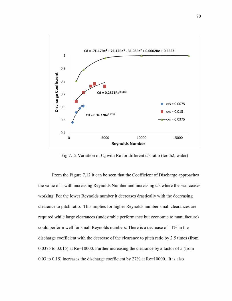
70
Fig 7.12 Variation of Cd with Re for different c/s ratio (tooth2, water)
From the Figure 7.12 it can be seen that the Coefficient of Discharge approaches
the value of 1 with increasing Reynolds Number and increasing c/s where the seal ceases
working. For the lower Reynolds number it decreases drastically with the decreasing
clearance to pitch ratio. This implies for higher Reynolds number small clearances are
required while large clearances (undesirable performance but economic to manufacture)
could perform well for small Reynolds numbers. There is a decrease of 11% in the
discharge coefficient with the decrease of the clearance to pitch ratio by 2.5 times (from
0.0375 to 0.015) at Re=10000. Further increasing the clearance by a factor of 5 (from
0.03 to 0.15) increases the discharge coefficient by 27% at Re=10000. It is also
Cd = 0.1677Re0.1714
Cd = 0.2871Re0.1193
Cd = -7E-17Re4 + 2E-12Re3 - 3E-08Re2 + 0.0002Re + 0.6662
0.4
0.5
0.6
0.7
0.8
0.9
1
0 5000 10000 15000
Dis
char
ge C
oef
fici
ent
Reynolds Number
c/s = 0.0075
c/s = 0.015
c/s = 0.0375
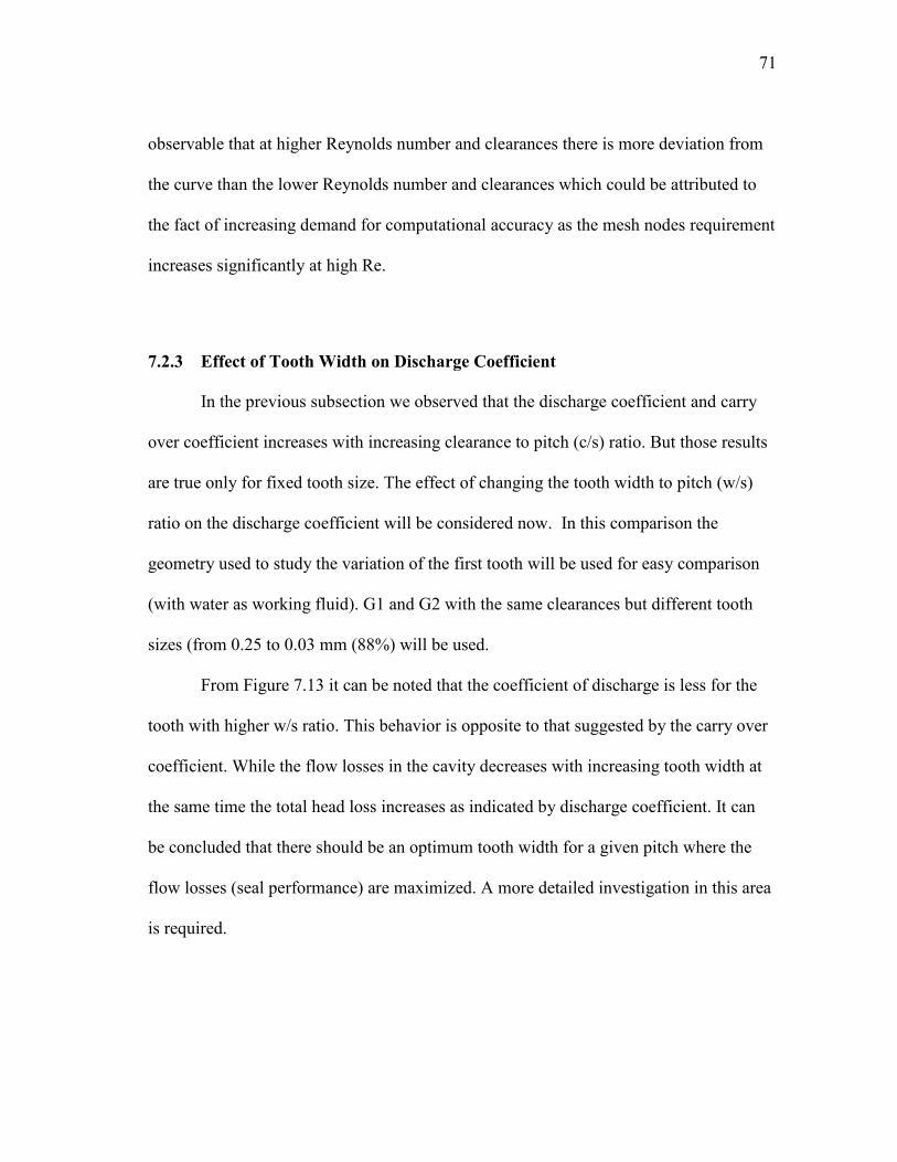
71
observable that at higher Reynolds number and clearances there is more deviation from
the curve than the lower Reynolds number and clearances which could be attributed to
the fact of increasing demand for computational accuracy as the mesh nodes requirement
increases significantly at high Re.
7.2.3 Effect of Tooth Width on Discharge Coefficient
In the previous subsection we observed that the discharge coefficient and carry
over coefficient increases with increasing clearance to pitch (c/s) ratio. But those results
are true only for fixed tooth size. The effect of changing the tooth width to pitch (w/s)
ratio on the discharge coefficient will be considered now. In this comparison the
geometry used to study the variation of the first tooth will be used for easy comparison
(with water as working fluid). G1 and G2 with the same clearances but different tooth
sizes (from 0.25 to 0.03 mm (88%) will be used.
From Figure 7.13 it can be noted that the coefficient of discharge is less for the
tooth with higher w/s ratio. This behavior is opposite to that suggested by the carry over
coefficient. While the flow losses in the cavity decreases with increasing tooth width at
the same time the total head loss increases as indicated by discharge coefficient. It can
be concluded that there should be an optimum tooth width for a given pitch where the
flow losses (seal performance) are maximized. A more detailed investigation in this area
is required.
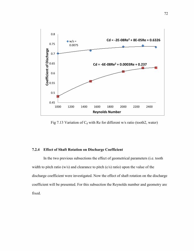
72
Fig 7.13 Variation of Cd with Re for different w/s ratio (tooth2, water)
7.2.4 Effect of Shaft Rotation on Discharge Coefficient
In the two previous subsections the effect of geometrical parameters (i.e. tooth
width to pitch ratio (w/s) and clearance to pitch (c/s) ratio) upon the value of the
discharge coefficient were investigated. Now the effect of shaft rotation on the discharge
coefficient will be presented. For this subsection the Reynolds number and geometry are
fixed.
Cd = -2E-08Re2 + 8E-05Re + 0.6326
Cd = -6E-08Re2 + 0.0003Re + 0.237
0.45
0.5
0.55
0.6
0.65
0.7
0.75
0.8
1000 1200 1400 1600 1800 2000 2200 2400
Co
effi
cien
t o
f D
isch
arge
Reynolds Number
w/s =0.0075
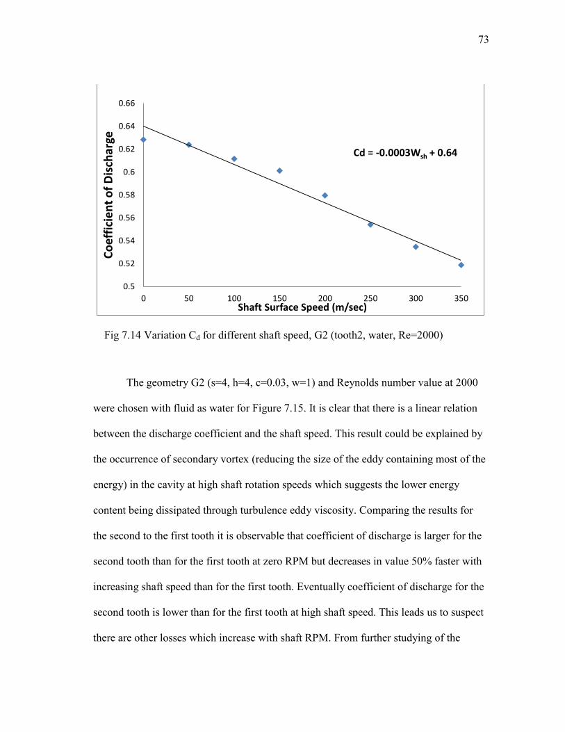
73
Fig 7.14 Variation Cd for different shaft speed, G2 (tooth2, water, Re=2000)
The geometry G2 (s=4, h=4, c=0.03, w=1) and Reynolds number value at 2000
were chosen with fluid as water for Figure 7.15. It is clear that there is a linear relation
between the discharge coefficient and the shaft speed. This result could be explained by
the occurrence of secondary vortex (reducing the size of the eddy containing most of the
energy) in the cavity at high shaft rotation speeds which suggests the lower energy
content being dissipated through turbulence eddy viscosity. Comparing the results for
the second to the first tooth it is observable that coefficient of discharge is larger for the
second tooth than for the first tooth at zero RPM but decreases in value 50% faster with
increasing shaft speed than for the first tooth. Eventually coefficient of discharge for the
second tooth is lower than for the first tooth at high shaft speed. This leads us to suspect
there are other losses which increase with shaft RPM. From further studying of the
Cd = -0.0003Wsh + 0.64
0.5
0.52
0.54
0.56
0.58
0.6
0.62
0.64
0.66
0 50 100 150 200 250 300 350
Co
effi
cie
nt
of
Dis
char
ge
Shaft Surface Speed (m/sec)
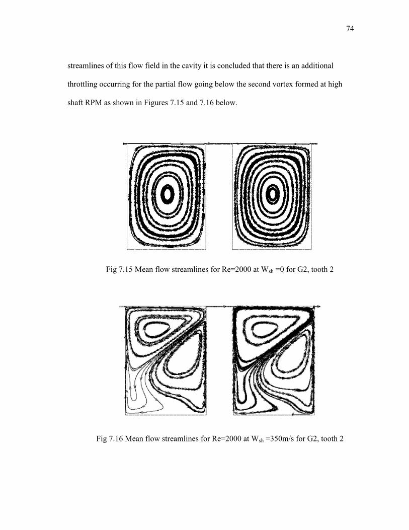
74
streamlines of this flow field in the cavity it is concluded that there is an additional
throttling occurring for the partial flow going below the second vortex formed at high
shaft RPM as shown in Figures 7.15 and 7.16 below.
Fig 7.15 Mean flow streamlines for Re=2000 at Wsh =0 for G2, tooth 2
Fig 7.16 Mean flow streamlines for Re=2000 at Wsh =350m/s for G2, tooth 2
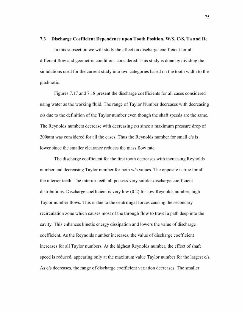
75
7.3 Discharge Coefficient Dependence upon Tooth Position, W/S, C/S, Ta and Re
In this subsection we will study the effect on discharge coefficient for all
different flow and geometric conditions considered. This study is done by dividing the
simulations used for the current study into two categories based on the tooth width to the
pitch ratio.
Figures 7.17 and 7.18 present the discharge coefficients for all cases considered
using water as the working fluid. The range of Taylor Number decreases with decreasing
c/s due to the definition of the Taylor number even though the shaft speeds are the same.
The Reynolds numbers decrease with decreasing c/s since a maximum pressure drop of
200atm was considered for all the cases. Thus the Reynolds number for small c/s is
lower since the smaller clearance reduces the mass flow rate.
The discharge coefficient for the first tooth decreases with increasing Reynolds
number and decreasing Taylor number for both w/s values. The opposite is true for all
the interior teeth. The interior teeth all possess very similar discharge coefficient
distributions. Discharge coefficient is very low (0.2) for low Reynolds number, high
Taylor number flows. This is due to the centrifugal forces causing the secondary
recirculation zone which causes most of the through flow to travel a path deep into the
cavity. This enhances kinetic energy dissipation and lowers the value of discharge
coefficient. As the Reynolds number increases, the value of discharge coefficient
increases for all Taylor numbers. At the highest Reynolds number, the effect of shaft
speed is reduced, appearing only at the maximum value Taylor number for the largest c/s.
As c/s decreases, the range of discharge coefficient variation decreases. The smaller
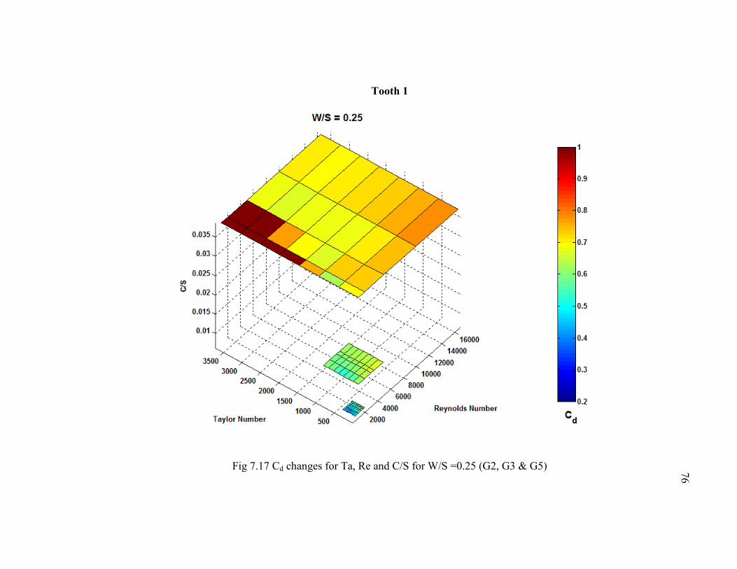
76
Tooth 1
Fig 7.17 Cd changes for Ta, Re and C/S for W/S =0.25 (G2, G3 & G5)
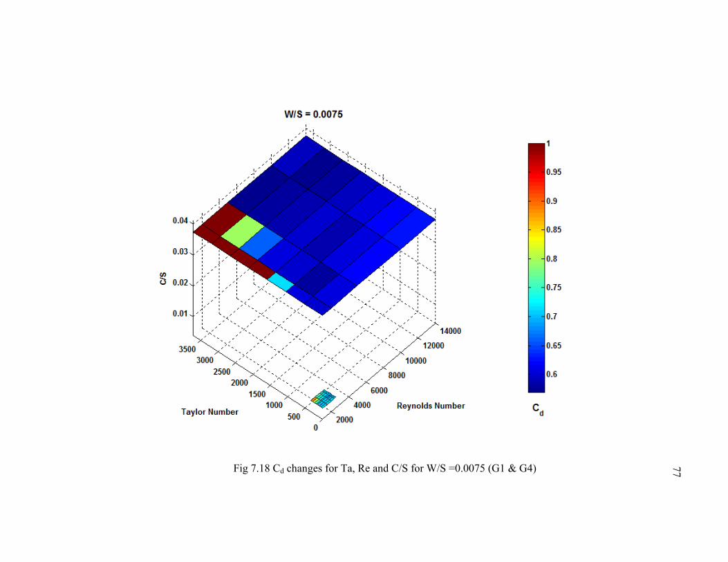
77
Fig 7.18 Cd changes for Ta, Re and C/S for W/S =0.0075 (G1 & G4)
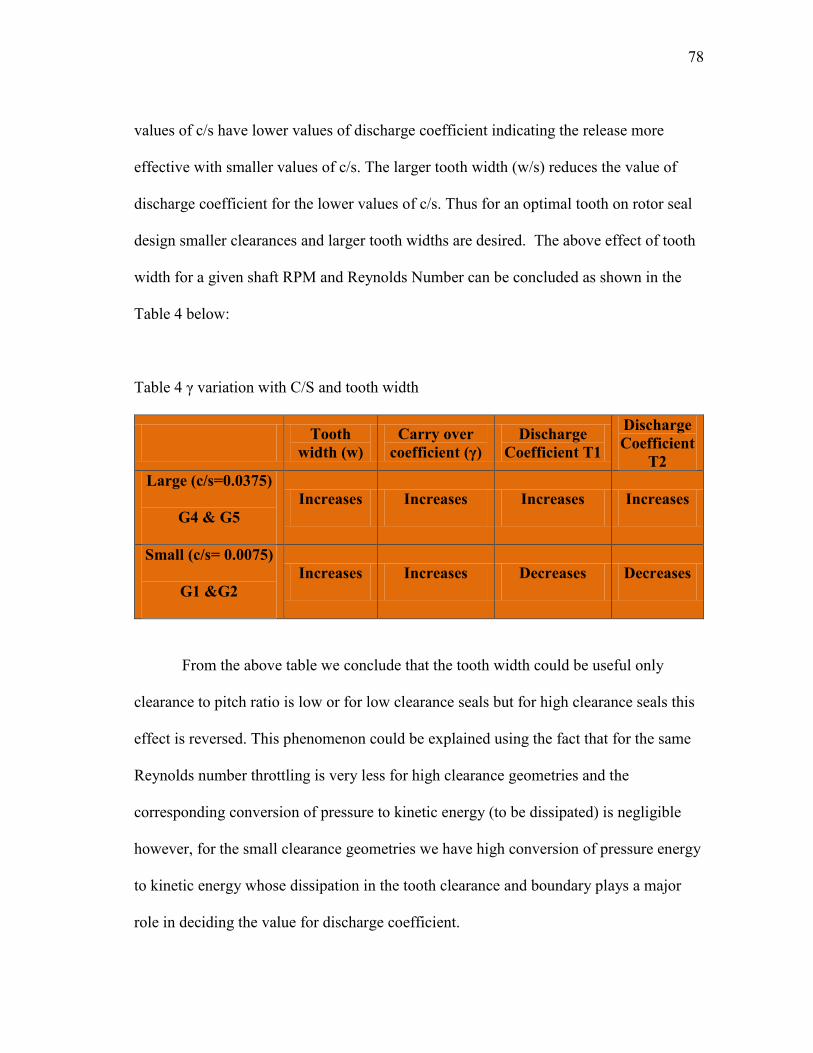
78
values of c/s have lower values of discharge coefficient indicating the release more
effective with smaller values of c/s. The larger tooth width (w/s) reduces the value of
discharge coefficient for the lower values of c/s. Thus for an optimal tooth on rotor seal
design smaller clearances and larger tooth widths are desired. The above effect of tooth
width for a given shaft RPM and Reynolds Number can be concluded as shown in the
Table 4 below:
Table 4 γ variation with C/S and tooth width
Tooth
width (w)
Carry over
coefficient (γ)
Discharge
Coefficient T1
Discharge
Coefficient
T2
Large (c/s=0.0375)
G4 & G5
Increases Increases Increases Increases
Small (c/s= 0.0075)
G1 &G2
Increases Increases Decreases Decreases
From the above table we conclude that the tooth width could be useful only
clearance to pitch ratio is low or for low clearance seals but for high clearance seals this
effect is reversed. This phenomenon could be explained using the fact that for the same
Reynolds number throttling is very less for high clearance geometries and the
corresponding conversion of pressure to kinetic energy (to be dissipated) is negligible
however, for the small clearance geometries we have high conversion of pressure energy
to kinetic energy whose dissipation in the tooth clearance and boundary plays a major
role in deciding the value for discharge coefficient.
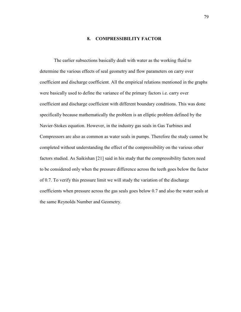
79
8. COMPRESSIBILITY FACTOR
The earlier subsections basically dealt with water as the working fluid to
determine the various effects of seal geometry and flow parameters on carry over
coefficient and discharge coefficient. All the empirical relations mentioned in the graphs
were basically used to define the variance of the primary factors i.e. carry over
coefficient and discharge coefficient with different boundary conditions. This was done
specifically because mathematically the problem is an elliptic problem defined by the
Navier-Stokes equation. However, in the industry gas seals in Gas Turbines and
Compressors are also as common as water seals in pumps. Therefore the study cannot be
completed without understanding the effect of the compressibility on the various other
factors studied. As Saikishan [21] said in his study that the compressibility factors need
to be considered only when the pressure difference across the teeth goes below the factor
of 0.7. To verify this pressure limit we will study the variation of the discharge
coefficients when pressure across the gas seals goes below 0.7 and also the water seals at
the same Reynolds Number and Geometry.
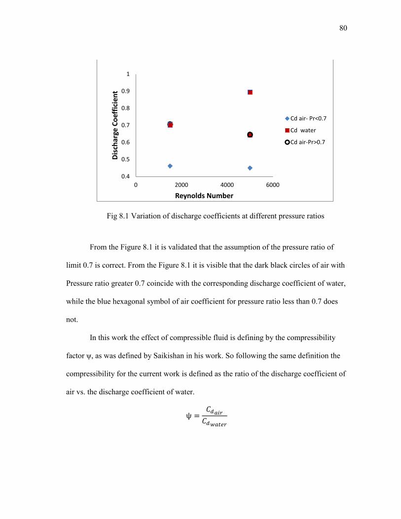
80
Fig 8.1 Variation of discharge coefficients at different pressure ratios
From the Figure 8.1 it is validated that the assumption of the pressure ratio of
limit 0.7 is correct. From the Figure 8.1 it is visible that the dark black circles of air with
Pressure ratio greater 0.7 coincide with the corresponding discharge coefficient of water,
while the blue hexagonal symbol of air coefficient for pressure ratio less than 0.7 does
not.
In this work the effect of compressible fluid is defining by the compressibility
factor ψ, as was defined by Saikishan in his work. So following the same definition the
compressibility for the current work is defined as the ratio of the discharge coefficient of
air vs. the discharge coefficient of water.
ψ
0.4
0.5
0.6
0.7
0.8
0.9
1
0 2000 4000 6000
Dis
char
ge C
oef
fici
ent
Reynolds Number
Cd air- Pr<0.7
Cd water
Cd air-Pr>0.7
81
This definition by itself considers the effect on compressibility on carry over
coefficient because we have included that in the definition of the discharge coefficient.
In many other previous works we do find the definition of compressibility following the
same trend as including here by Hodkinson [3], Vermes [18]. All the people who used
the Martin‟s basic equation added different coefficients to determine the compressibility
factor either empirically or on the basis of some hypothesis. Truly none of them
accurately defined the compressibility factor earlier because either the assumptions made
were wrong and also the disability to correctly solve the turbulent flow regime whose
accuracy cannot be more than the CFD solver code used to solve them. Further we are
going to analyze the effects of various non- dimensional fluid and geometrical
parameters on the compressibility factor as we did for the carry over and discharge
coefficients earlier.
8.1 Effect of Position of Tooth on the Compressibility Factor
Figure 8.2 shows the effect of compressibility for both the first tooth and the
second tooth. The need for this study arises after coming across the difference in the
value of the discharge coefficient. Also, as the absolute pressure in each seal cavity
decreases in the downstream direction, the pressure ratio increases. The minimum value
usually occurs at the last tooth where the flow may be choked.
.
82
Fig 8.2 Variation of compressibility factor with tooth position
From the above Figure 8.2 it is clearly visible that the compressibility factor
variation is negligible with the tooth position so it becomes valid that the relations that
would be found between flow parameters and geometrical parameters on compressibility
will be valid for the entire teeth series similarly. So this eliminates the need to separately
analyze the first tooth from the other teeth on the labyrinth seals for all the parameters
suspected to change it.
8.2 Effect of Flow Parameters on Compressibility Factor
As stated in all the earlier studies, compressibility has been shown to be a major
function of pressure ratio (here we refer to the absolute pressure ratio across the tooth
rather than across the whole seal).
0
0.2
0.4
0.6
0.8
1
1.2
0 0.2 0.4 0.6 0.8 1
Co
mp
ress
ibili
ty F
acto
r
Pressure Ratio
Inner Tooth
First Tooth
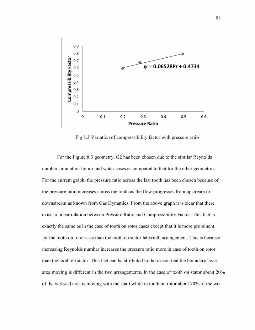
83
Fig 8.3 Variation of compressibility factor with pressure ratio
For the Figure 8.3 geometry, G2 has been chosen due to the similar Reynolds
number simulation for air and water cases as compared to that for the other geometries.
For the current graph, the pressure ratio across the last tooth has been chosen because of
the pressure ratio increases across the tooth as the flow progresses from upstream to
downstream as known from Gas Dynamics. From the above graph it is clear that there
exists a linear relation between Pressure Ratio and Compressibility Factor. This fact is
exactly the same as in the case of tooth on rotor cases except that it is more prominent
for the tooth on rotor case than the tooth on stator labyrinth arrangement. This is because
increasing Reynolds number increases the pressure ratio more in case of tooth on rotor
than the tooth on stator. This fact can be attributed to the reason that the boundary layer
area moving is different in the two arrangements. In the case of tooth on stator about 20%
of the wet seal area is moving with the shaft while in tooth on rotor about 70% of the wet
ψ = 0.06528Pr + 0.4734
0
0.1
0.2
0.3
0.4
0.5
0.6
0.7
0.8
0.9
0 0.1 0.2 0.3 0.4 0.5 0.6
Co
mp
ress
ibili
ty F
acto
r
Pressure Ratio
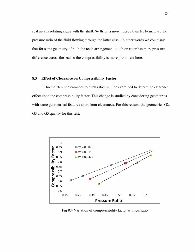
84
seal area is rotating along with the shaft. So there is more energy transfer to increase the
pressure ratio of the fluid flowing through the latter case. In other words we could say
that for same geometry of both the teeth arrangement, tooth on rotor has more pressure
difference across the seal so the compressibility is more prominent here.
8.3 Effect of Clearance on Compressibility Factor
Three different clearances to pitch ratios will be examined to determine clearance
effect upon the compressibility factor. This change is studied by considering geometries
with same geometrical features apart from clearances. For this reason, the geometries G2,
G3 and G5 qualify for this test.
Fig 8.4 Variation of compressibility factor with c/s ratio
0.5
0.55
0.6
0.65
0.7
0.75
0.8
0.85
0.9
0.95
1
0.15 0.25 0.35 0.45 0.55 0.65 0.75
Co
mp
ress
ibili
ty F
acto
r
Pressure Ratio
c/s = 0.0075
c/s = 0.015
c/s = 0.0375
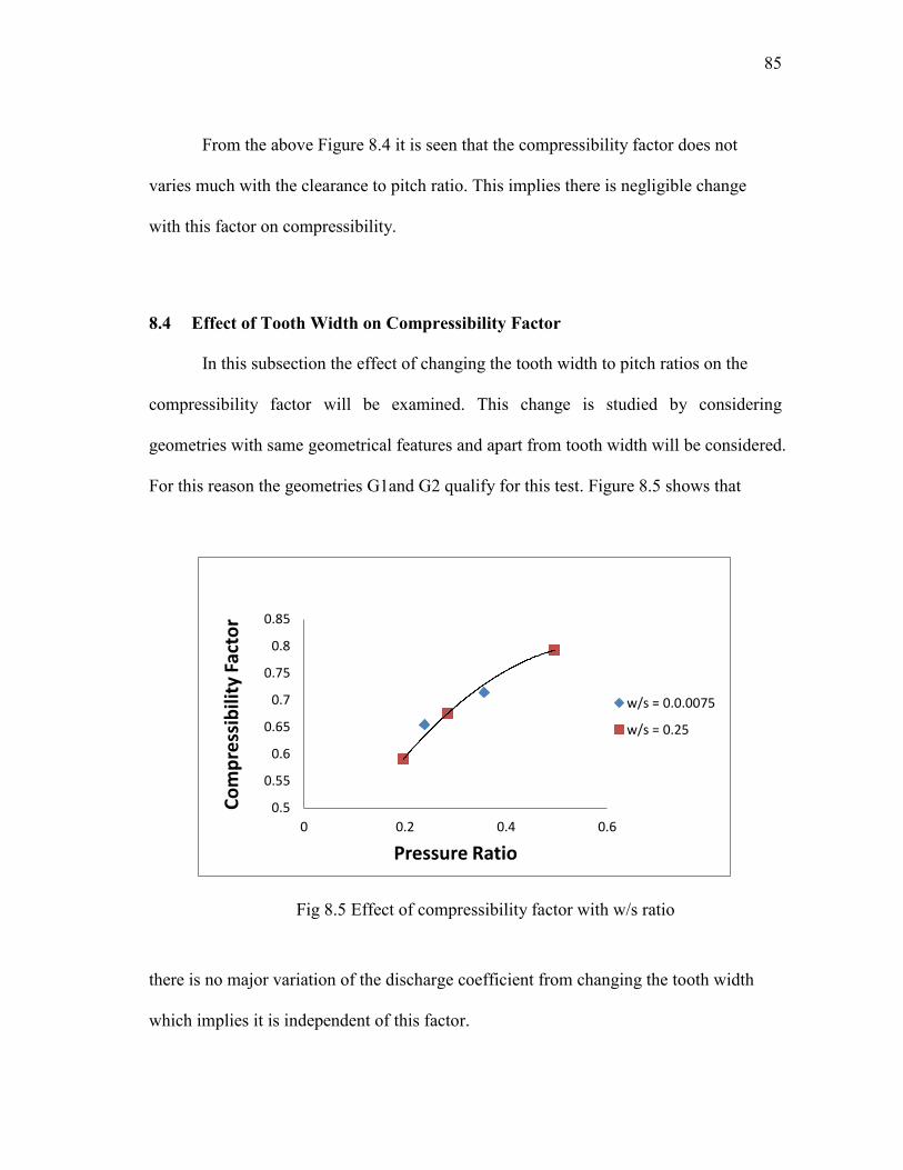
85
From the above Figure 8.4 it is seen that the compressibility factor does not
varies much with the clearance to pitch ratio. This implies there is negligible change
with this factor on compressibility.
8.4 Effect of Tooth Width on Compressibility Factor
In this subsection the effect of changing the tooth width to pitch ratios on the
compressibility factor will be examined. This change is studied by considering
geometries with same geometrical features and apart from tooth width will be considered.
For this reason the geometries G1and G2 qualify for this test. Figure 8.5 shows that
Fig 8.5 Effect of compressibility factor with w/s ratio
there is no major variation of the discharge coefficient from changing the tooth width
which implies it is independent of this factor.
0.5
0.55
0.6
0.65
0.7
0.75
0.8
0.85
0 0.2 0.4 0.6
Co
mp
ress
ibili
ty F
acto
r
Pressure Ratio
w/s = 0.0.0075
w/s = 0.25
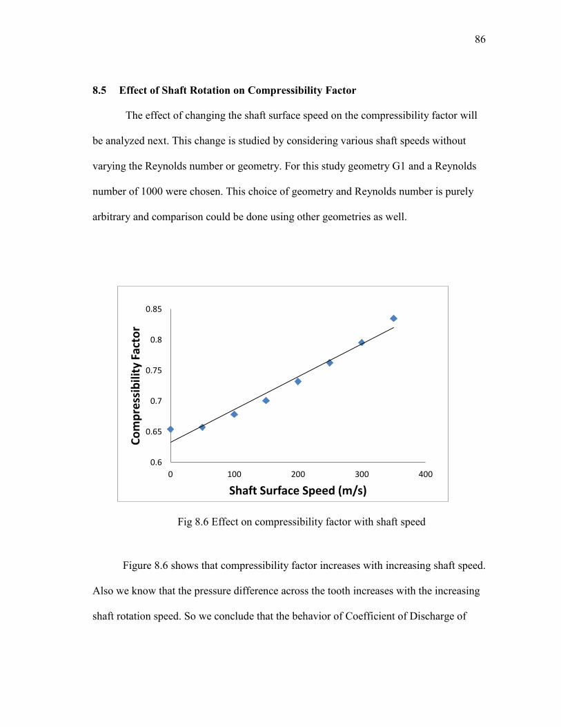
86
8.5 Effect of Shaft Rotation on Compressibility Factor
The effect of changing the shaft surface speed on the compressibility factor will
be analyzed next. This change is studied by considering various shaft speeds without
varying the Reynolds number or geometry. For this study geometry G1 and a Reynolds
number of 1000 were chosen. This choice of geometry and Reynolds number is purely
arbitrary and comparison could be done using other geometries as well.
Fig 8.6 Effect on compressibility factor with shaft speed
Figure 8.6 shows that compressibility factor increases with increasing shaft speed.
Also we know that the pressure difference across the tooth increases with the increasing
shaft rotation speed. So we conclude that the behavior of Coefficient of Discharge of
0.6
0.65
0.7
0.75
0.8
0.85
0 100 200 300 400
Co
mp
ress
ibili
ty F
acto
r
Shaft Surface Speed (m/s)
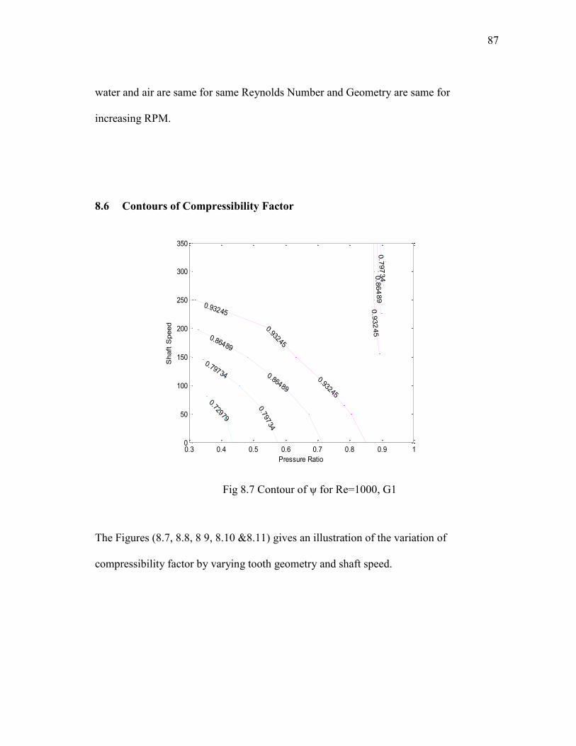
87
water and air are same for same Reynolds Number and Geometry are same for
increasing RPM.
8.6 Contours of Compressibility Factor
Fig 8.7 Contour of ψ for Re=1000, G1
The Figures (8.7, 8.8, 8 9, 8.10 &8.11) gives an illustration of the variation of
compressibility factor by varying tooth geometry and shaft speed.
0.72979
0.7
97
34
0.7
9734
0.79734
0.8
64
89
0.86489
0.86489
0.9
32
45
0.93245
0.93245
0.93245
Pressure Ratio
Shaft
Speed
0.3 0.4 0.5 0.6 0.7 0.8 0.9 10
50
100
150
200
250
300
350
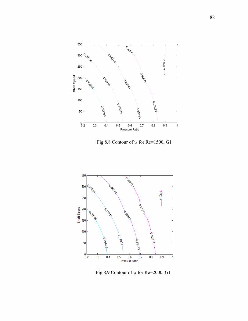
88
Fig 8.8 Contour of ψ for Re=1500, G1
Fig 8.9 Contour of ψ for Re=2000, G1
0.7
06
85
0.70685
0.7
80
14
0.78014
0.78014
0.85343
0.85343
0.8
53
43
0.9
26
71
0.9
26
71
0.9
2671
0.92671
Pressure Ratio
Shaft
Speed
0.2 0.3 0.4 0.5 0.6 0.7 0.8 0.9 10
50
100
150
200
250
300
350
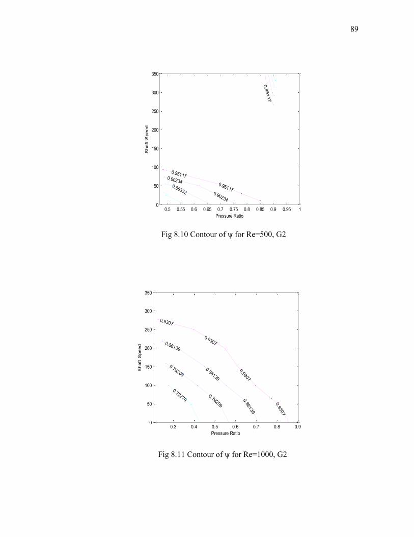
89
Fig 8.10 Contour of ψ for Re=500, G2
Fig 8.11 Contour of ψ for Re=1000, G2
0.85352 0.90234
0.90234
0.9
51
17
0.95117
0.95117
Pressure Ratio
Shaft
Speed
0.5 0.55 0.6 0.65 0.7 0.75 0.8 0.85 0.9 0.95 10
50
100
150
200
250
300
350
0.722790.79209
0.79209
0.86139
0.86139
0.86139
0.9
307
0.9307
0.9307
0.9307
Pressure Ratio
Shaft
Speed
0.3 0.4 0.5 0.6 0.7 0.8 0.90
50
100
150
200
250
300
350
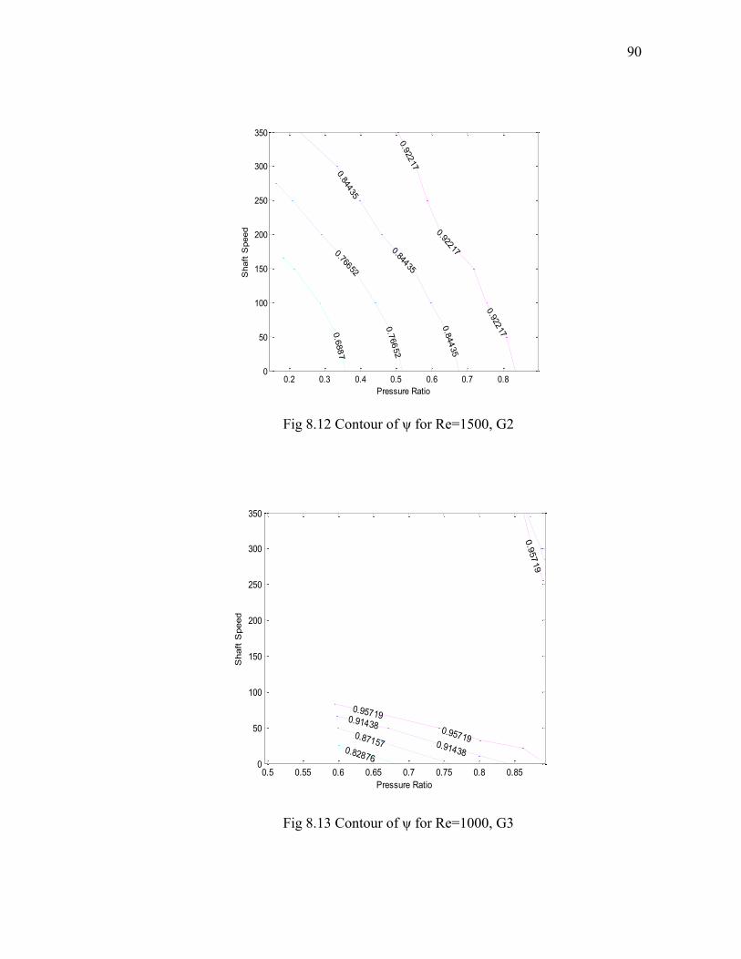
90
Fig 8.12 Contour of ψ for Re=1500, G2
Fig 8.13 Contour of ψ for Re=1000, G3
0.6
88
7
0.7
66
52
0.76652
0.84435
0.84435
0.8
44
35
0.9
2217
0.92217
0.9
2217
Pressure Ratio
Shaft
Speed
0.2 0.3 0.4 0.5 0.6 0.7 0.80
50
100
150
200
250
300
350
0.82876
0.87157 0.91438
0.91438
0.9
57
19
0.95719
0.95719
Pressure Ratio
Shaft
Speed
0.5 0.55 0.6 0.65 0.7 0.75 0.8 0.850
50
100
150
200
250
300
350
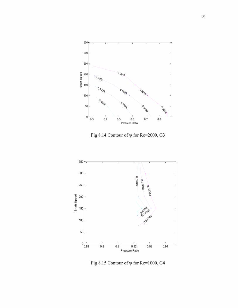
91
Fig 8.14 Contour of ψ for Re=2000, G3
Fig 8.15 Contour of ψ for Re=1000, G4
0.69840.7738
0.7738
0.8492
0.8492
0.84920.924
6
0.9246
0.9246
Pressure Ratio
Shaft
Speed
0.3 0.4 0.5 0.6 0.7 0.80
50
100
150
200
250
300
350
0.6
20
3
0.62
03
0.7
46
87
0.74687
0.8
73
43
0.87
343
Pressure Ratio
Shaft
Speed
0.89 0.9 0.91 0.92 0.93 0.940
50
100
150
200
250
300
350
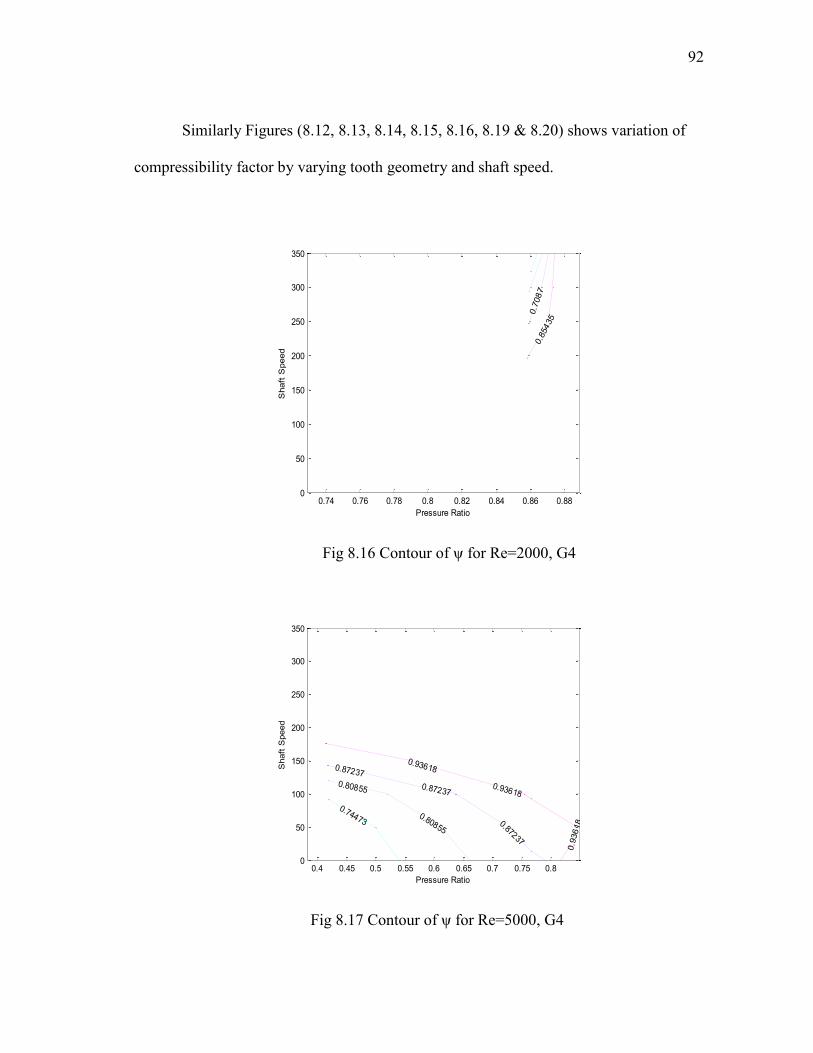
92
Similarly Figures (8.12, 8.13, 8.14, 8.15, 8.16, 8.19 & 8.20) shows variation of
compressibility factor by varying tooth geometry and shaft speed.
Fig 8.16 Contour of ψ for Re=2000, G4
Fig 8.17 Contour of ψ for Re=5000, G4
0.7
08
70.8
5435
Pressure Ratio
Shaft
Speed
0.74 0.76 0.78 0.8 0.82 0.84 0.86 0.880
50
100
150
200
250
300
350
0.744730.80855
0.80855
0.87237
0.87237
0.87237
0.9
36
18
0.93618
0.93618
Pressure Ratio
Shaft
Speed
0.4 0.45 0.5 0.55 0.6 0.65 0.7 0.75 0.80
50
100
150
200
250
300
350
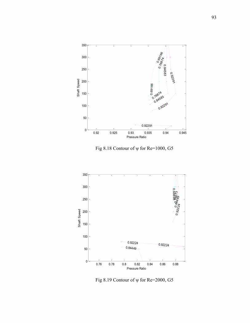
93
Fig 8.18 Contour of ψ for Re=1000, G5
Fig 8.19 Contour of ψ for Re=2000, G5
0.6
91
66
0.6
91
66
0.7
68
74
0.76874
0.8
45
83
0.84583
0.9
22
91
0.92291
0.92291
Pressure Ratio
Shaft
Speed
0.92 0.925 0.93 0.935 0.94 0.9450
50
100
150
200
250
300
350
0.6
88
98
0.7
66
73
0.8
44
49
0.84449
0.9
22
24
0.922240.92224
Pressure Ratio
Shaft
Speed
0.76 0.78 0.8 0.82 0.84 0.86 0.880
50
100
150
200
250
300
350
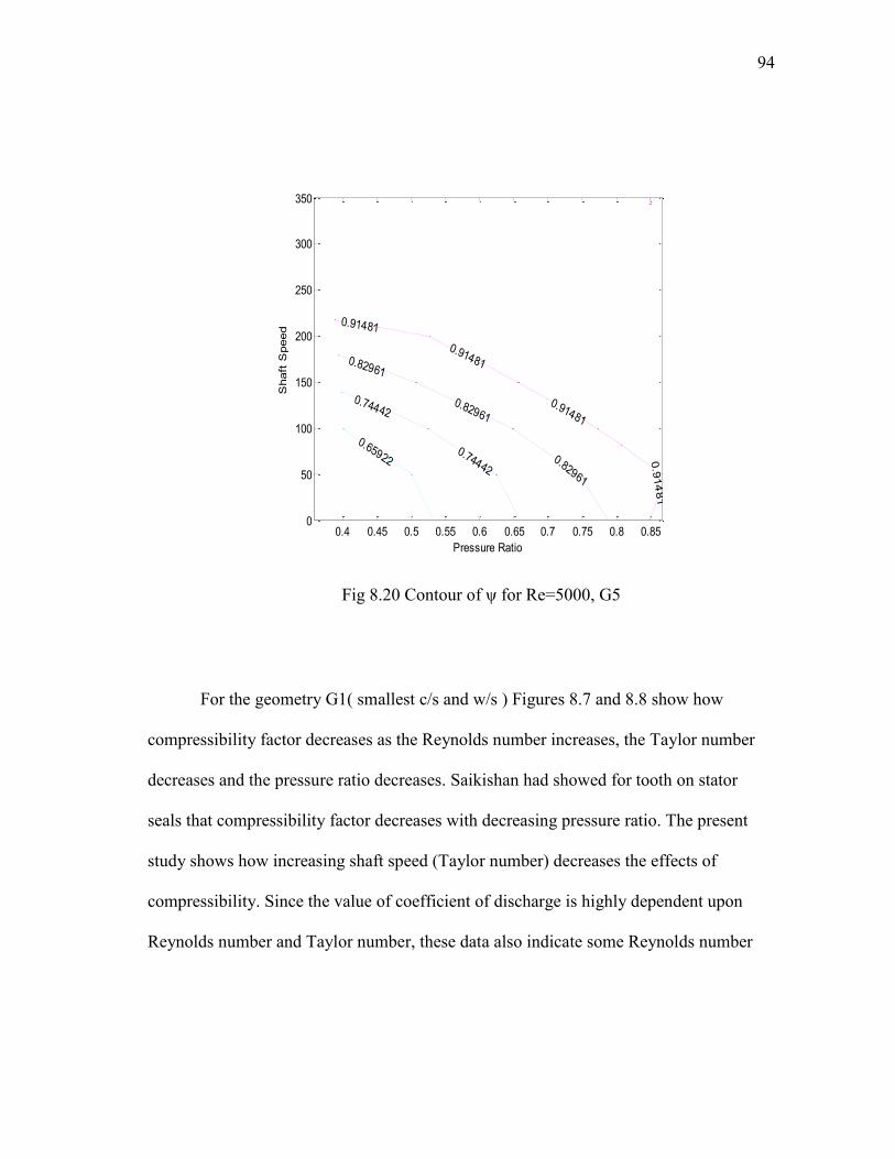
94
Fig 8.20 Contour of ψ for Re=5000, G5
For the geometry G1( smallest c/s and w/s ) Figures 8.7 and 8.8 show how
compressibility factor decreases as the Reynolds number increases, the Taylor number
decreases and the pressure ratio decreases. Saikishan had showed for tooth on stator
seals that compressibility factor decreases with decreasing pressure ratio. The present
study shows how increasing shaft speed (Taylor number) decreases the effects of
compressibility. Since the value of coefficient of discharge is highly dependent upon
Reynolds number and Taylor number, these data also indicate some Reynolds number
0.659220.74442
0.74442
0.82961
0.82961
0.82961
0.9
14
81
0.91481
0.91481
0.91481
Pressure Ratio
Shaft
Speed
0.4 0.45 0.5 0.55 0.6 0.65 0.7 0.75 0.8 0.850
50
100
150
200
250
300
350
95
dependence. This is due to the changing nature of the recirculation zone with the value
of Reynolds number and Taylor number.
Increasing the tooth width to pitch ratio to 0.25 (G2, Figures 8.10 to 8.12) at
same pressure ratio does not change the effects of compressibility (larger compressibility
factor values) tremendously. The effect of Taylor Number is also decreased with this
much wider tooth width. There is still a significant increase in compressibility factor as
Reynolds number increases. This further confirms that the pressure ratio is the only
governing factor which changes the compressibility.
Maintaining the large tooth width and increasing the seal clearance to pitch ratio
(G3, w/s =0.25 and c/s=0.015) compressibility factors is decreases slightly. This implies
an increment in compressibility. Taylor number dependence is further reduced.
The two geometries with largest clearance to pitch ratio cases G4 (w/s =0.0075
and c/s=0.0375) and G5 (w/s =0.25 and c/s=0.0375) had minimized data obtained at
lower Reynolds numbers as indicated by the small regions of contours. The
compressibility factor is also changing at a comparatively slower pace than that from the
geometries with smaller clearance to pitch ratio cases G1 (w/s =0.0075 and c/s=0.0075)
and G2 (w/s =0.25 and c/s=0.0075). Also to note that the effect of changing clearance to
pitch (c/s) is more pronounced than by changing tooth width to pitch (w/s) as visible
from Figures 8.7 and 8.15 for G1and G4 for Re=1000.
From the above discussions we conclude that compressibility is only a function
of pressure ratio which change by varying Taylor Number and Reynolds Number for a
flow field. Any change in geometry and boundary condition keeping pressure ratio
96
constant across tooth will not change the compressibility factor. This agrees well with
definition of compressibility factor which has been defined to take care of changing fluid
density (only a function of pressure and temperature for a given ideal working fluid.
Further it has been also confirmed that density ratios and pressure ratios across a tooth
are fairly same. This further supports the results obtained.
97
9. SUMMARY
9.1 Carry over Coefficient
The carry over coefficient was calculated using the divergence angle of the seal.
The definition given by Hodkinson was used to calculate the carry over coefficient. It
was found that it depends upon flow conditions, geometry of the seal and the changing
boundary conditions. It was found that for cases with water as working fluid carry over
coefficient does increase with Reynolds number. This increase is same in nature for the
case on stator arrangement. The tooth clearance to pitch (c/s) was determined to be the
major geometrical parameter to determine the carry over coefficient. It was observed that
the tooth width to pitch ratio (w/s) cannot be neglected at higher Reynolds number flow
where its effect is a major consideration. Shaft RPM effect was very complex which
suggests to study about the changing shear forces with changing flow field in the cavity
from one vortex to the complete generation of secondary vortex at high Taylor number.
By comparing all the factors it was concluded that Taylor number decreases at higher
carry over coefficient.
9.2 Discharge Coefficient
It is defined to calculate the total pressure loss in a labyrinth seal. This coefficient
was found to vary with the position of the teeth on the shaft. While the first tooth was
found to have more losses than the intermediate teeth as was for the teeth on stator
98
configuration. The discharge coefficient was found to increase with the Reynolds
number for a given geometry and shaft speed. Among the geometrical factors relation of
discharge coefficient with tooth clearance to pitch (c/s) was found at lower Reynolds
number which dies away with the increasing flow inertia. Tooth width to pitch ratio (w/s)
was also found to change discharge coefficient at low Reynolds number. Taylor number
increment also found to change discharge coefficient in the opposite direction.
9.3 Compressibility Factor
This factor is defined to correlate the flow losses of compressible fluid to
incompressible flow. It is calculated using the ratio of discharge coefficient for air to that
of water at the same Reynolds number for a given geometry and tooth. It was found to
be mainly dependent on shaft RPM and pressure ratio. While for the tooth width to
clearance ratio (w/s) and tooth width to clearance ratio (w/c) affects the compressibility
factor negligibly less. It is also found that tooth position also does not effect this value
but increases linearly with the shaft RPM.
9.4 Suggestible Tooth Configuration
So from this study we conclude that the most efficient tooth geometry is decided
by the shaft RPM in the following way. For stationary shaft we need to have small c/s
and low Reynolds Number. Further it could be divided into two cases using the Table 5
below:
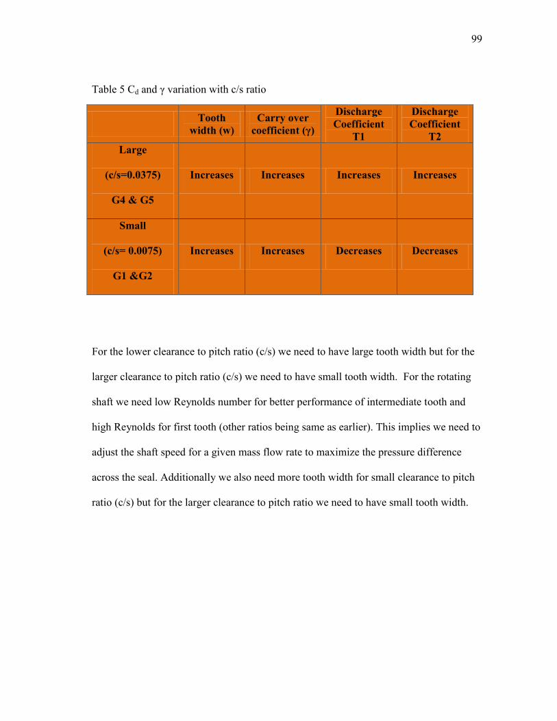
99
Table 5 Cd and γ variation with c/s ratio
Tooth
width (w)
Carry over
coefficient (γ)
Discharge
Coefficient
T1
Discharge
Coefficient
T2
Large
(c/s=0.0375)
G4 & G5
Increases Increases Increases Increases
Small
(c/s= 0.0075)
G1 &G2
Increases Increases Decreases Decreases
For the lower clearance to pitch ratio (c/s) we need to have large tooth width but for the
larger clearance to pitch ratio (c/s) we need to have small tooth width. For the rotating
shaft we need low Reynolds number for better performance of intermediate tooth and
high Reynolds for first tooth (other ratios being same as earlier). This implies we need to
adjust the shaft speed for a given mass flow rate to maximize the pressure difference
across the seal. Additionally we also need more tooth width for small clearance to pitch
ratio (c/s) but for the larger clearance to pitch ratio we need to have small tooth width.
100
10. RECOMMENDED FUTURE WORK AND CONCLUSION
The current research work has been done within few limitations and
simplifications. So there is a need of study the effects of these additional factors on the
flow field defining so that we could have a more versatile formulae for the application.
1. This study involves the study of tooth on the same shaft diameter. So we need to
further study the effect of changing the shaft diameter for the configuration of tooth on
rotor.
2. The current work involves the study of various teeth with different flow and geometric
limitations. So there is a need to explore the same effect with the increasing tooth
clearances and tooth width. This would help to understand more about the different seals
used in the industry which are not limited by the geometric and flow criteria of this study.
3. The current study uses ideal air as the compressible fluid for the study so we need to
explore the effect of the different real gases on the losses through the seals. This should
be incorporated with real gas equation where more accurate leakage results could be
derived for the real gas in application in various turbines and the compressors.
4. This study is limited to the straight through rectangular tooth on rotor. So there is a
need to explore the seals with different tooth geometries and different arrangements.
This includes staggered and stepped seals.
5. Different papers have done the fluid analysis work using various CFD turbulence
models. So there is a need to explore the changes in the results made by these different
101
turbulence models and compare them with the experimental results where shaft speed
goes higher than Mach 1. This might suggest a change in turbulence models with the
increasing shaft speed.
6. The viscosity of the fluid under high pressures such as 200 atm for water has been
considered to be constant. So an effort could also be made to see the variance in the
mass flow leakages with the variation of the fluid viscosity.
102
REFERENCES
[1] “The Labyrinth Packing” Engineer Vol. 165, 4280, Jan21, 1938, pp. 23-84.
[2] Manish, T., 2009, “Impact of Rotor Surface Velocity, Leakage Models and Real
Gas Properties on Rotor dynamic Force Predictions of Gas Labyrinth Seals,” M.S.
dissertation. Texas A&M University, College Station.
[3] Hodkinson, B., 1939, “Estimation of the Leakage Through a Labyrinth Gland,”
Proceedings of the Institution of Mechanical Engineers 141, pp. 283–288
[4] Becker, E. “Stromungsvergange in Ringformigen Spalten,” V.D.I., 51, 1907,
pp.1133-1141.
[5] Martin, H.M., Jan 19, 1908 , “Labyrinth Packings,”Engineering, pp 35-36.
[6] Stodola, A., 1927, Steam and Gas Turbines, 6th
ed., The McGraw-Hill Book
Company, New York.
[7] Dollin, F. and Brown, W.S., „Flow of Fluids Through Opening in Series,”
Engineer, 164, 4259, Aug 27, 1937, pp. 223-224.
[8] Gercke, M., 1934, “Flow Through Labyrinth Packing,” Mechanical Engineer, 56,
pp. 678-680.
[9] Elgi, A., 1935, “The Leakage of Steam Through Labyrinth Seals,” Trans. ASME,
57, pp. 115-122.
[10] Keller, C., 1937, “Flow Through Labyrinth Glands”, Power Plant Engineering, 41,
4, pp 243-245.
[11] Bell, K. J. and Bergelin, O.P., 1957(April), “Flow Through Annular Orifices,”
ASME Transactions, 79, 3, pp 593-601
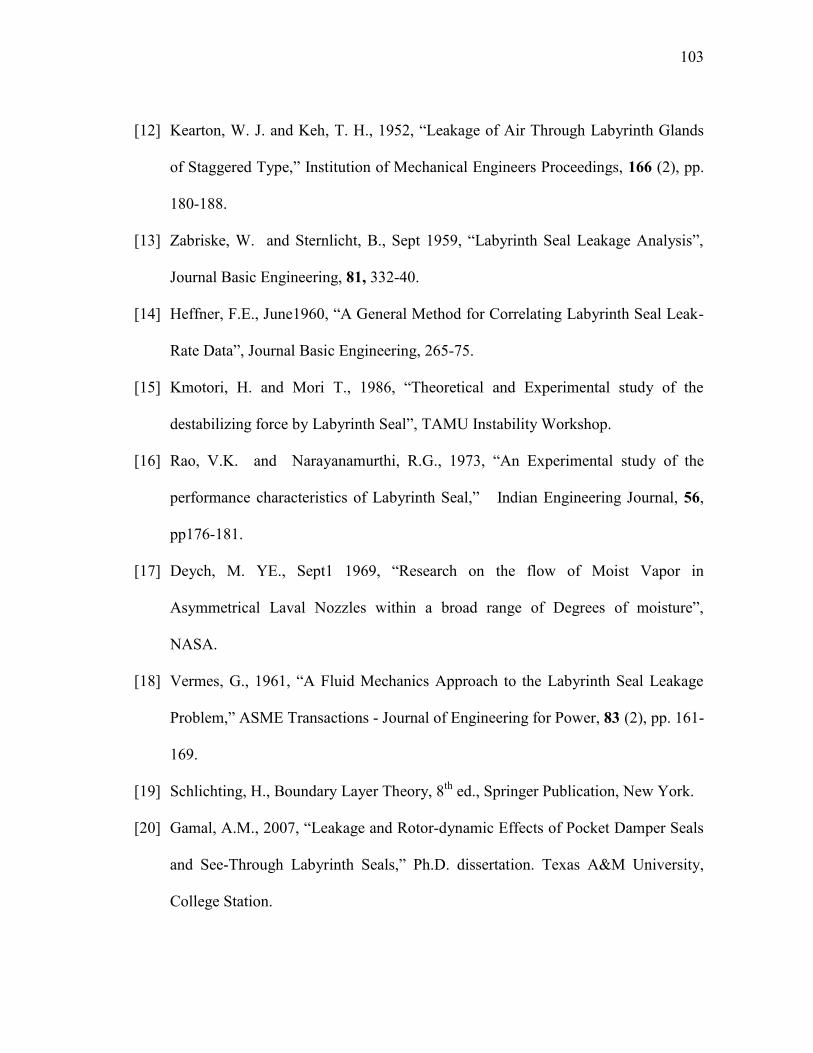
103
[12] Kearton, W. J. and Keh, T. H., 1952, “Leakage of Air Through Labyrinth Glands
of Staggered Type,” Institution of Mechanical Engineers Proceedings, 166 (2), pp.
180-188.
[13] Zabriske, W. and Sternlicht, B., Sept 1959, “Labyrinth Seal Leakage Analysis”,
Journal Basic Engineering, 81, 332-40.
[14] Heffner, F.E., June1960, “A General Method for Correlating Labyrinth Seal Leak-
Rate Data”, Journal Basic Engineering, 265-75.
[15] Kmotori, H. and Mori T., 1986, “Theoretical and Experimental study of the
destabilizing force by Labyrinth Seal”, TAMU Instability Workshop.
[16] Rao, V.K. and Narayanamurthi, R.G., 1973, “An Experimental study of the
performance characteristics of Labyrinth Seal,” Indian Engineering Journal, 56,
pp176-181.
[17] Deych, M. YE., Sept1 1969, “Research on the flow of Moist Vapor in
Asymmetrical Laval Nozzles within a broad range of Degrees of moisture”,
NASA.
[18] Vermes, G., 1961, “A Fluid Mechanics Approach to the Labyrinth Seal Leakage
Problem,” ASME Transactions - Journal of Engineering for Power, 83 (2), pp. 161-
169.
[19] Schlichting, H., Boundary Layer Theory, 8th
ed., Springer Publication, New York.
[20] Gamal, A.M., 2007, “Leakage and Rotor-dynamic Effects of Pocket Damper Seals
and See-Through Labyrinth Seals,” Ph.D. dissertation. Texas A&M University,
College Station.
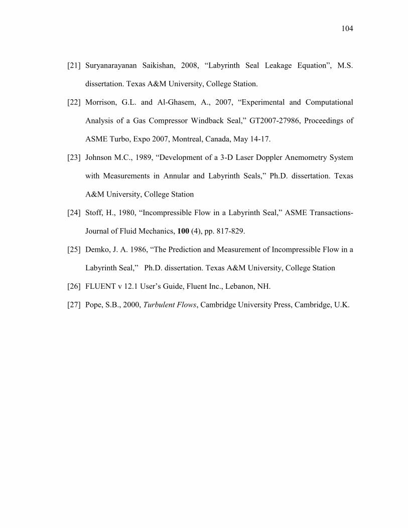
104
[21] Suryanarayanan Saikishan, 2008, “Labyrinth Seal Leakage Equation”, M.S.
dissertation. Texas A&M University, College Station.
[22] Morrison, G.L. and Al-Ghasem, A., 2007, “Experimental and Computational
Analysis of a Gas Compressor Windback Seal,” GT2007-27986, Proceedings of
ASME Turbo, Expo 2007, Montreal, Canada, May 14-17.
[23] Johnson M.C., 1989, “Development of a 3-D Laser Doppler Anemometry System
with Measurements in Annular and Labyrinth Seals,” Ph.D. dissertation. Texas
A&M University, College Station
[24] Stoff, H., 1980, “Incompressible Flow in a Labyrinth Seal,” ASME Transactions-
Journal of Fluid Mechanics, 100 (4), pp. 817-829.
[25] Demko, J. A. 1986, “The Prediction and Measurement of Incompressible Flow in a
Labyrinth Seal,” Ph.D. dissertation. Texas A&M University, College Station
[26] FLUENT v 12.1 User‟s Guide, Fluent Inc., Lebanon, NH.
[27] Pope, S.B., 2000, Turbulent Flows, Cambridge University Press, Cambridge, U.K.
105
APPENDIX
Cavity 2
Fig A.1 γ changes with Ta, Re and C/S for W/S =0.25 (G2, G3 & G5)
106
Fig A.2 γ changes with Ta, Re and C/S for W/S =0.0075 (G1 & G4)
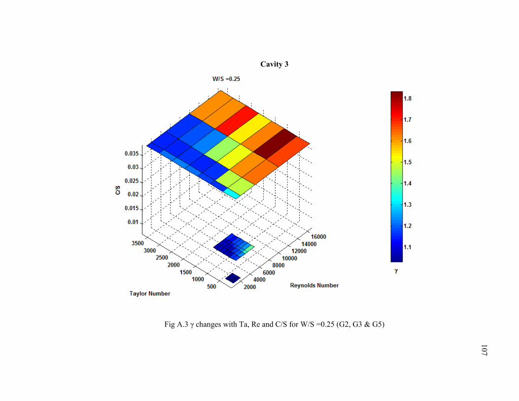
107
Cavity 3
Fig A.3 γ changes with Ta, Re and C/S for W/S =0.25 (G2, G3 & G5)
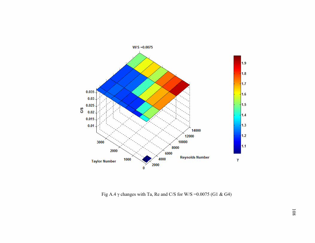
108
Fig A.4 γ changes with Ta, Re and C/S for W/S =0.0075 (G1 & G4)
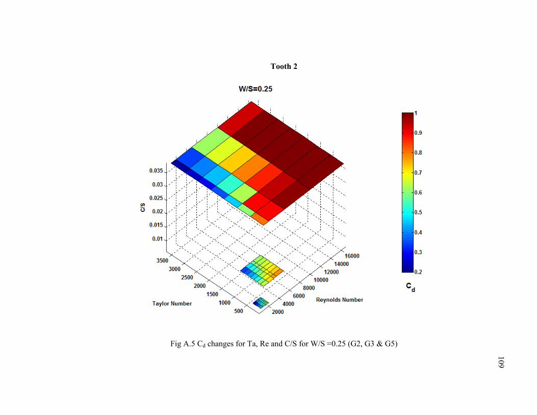
109
Tooth 2
Fig A.5 Cd changes for Ta, Re and C/S for W/S =0.25 (G2, G3 & G5)
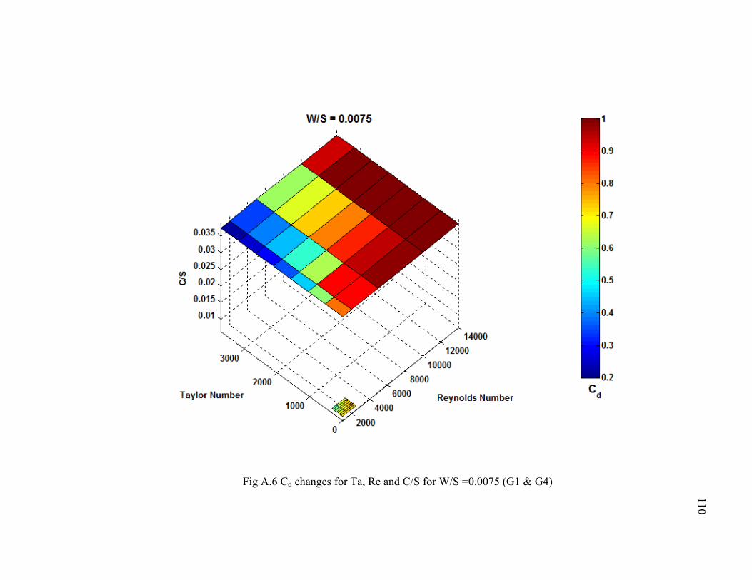
110
Fig A.6 Cd changes for Ta, Re and C/S for W/S =0.0075 (G1 & G4)
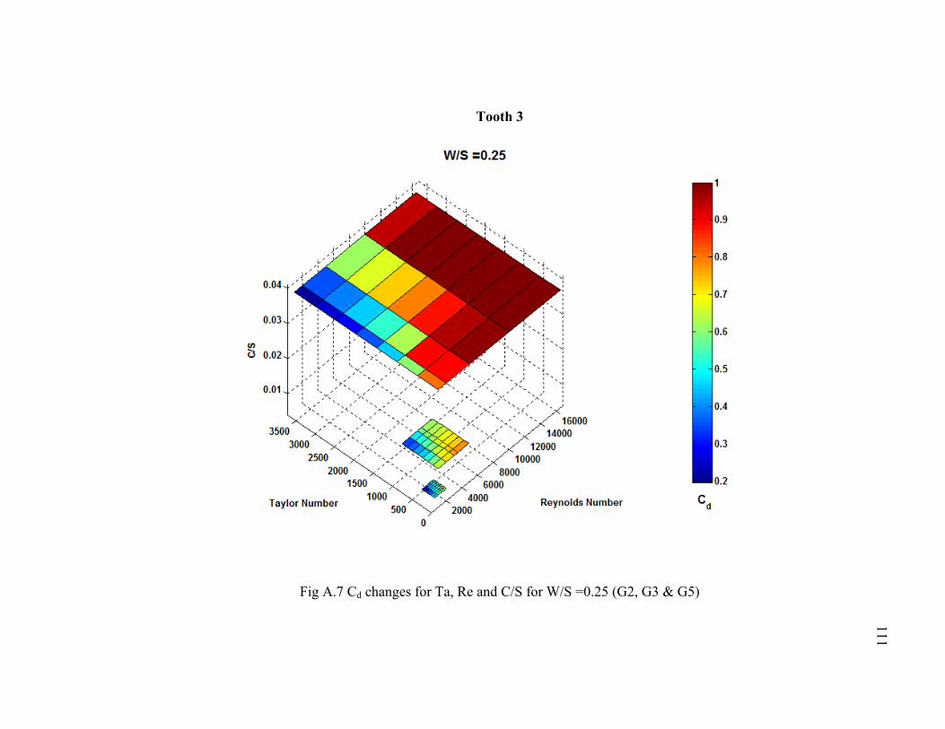
111
Tooth 3
Fig A.7 Cd changes for Ta, Re and C/S for W/S =0.25 (G2, G3 & G5)
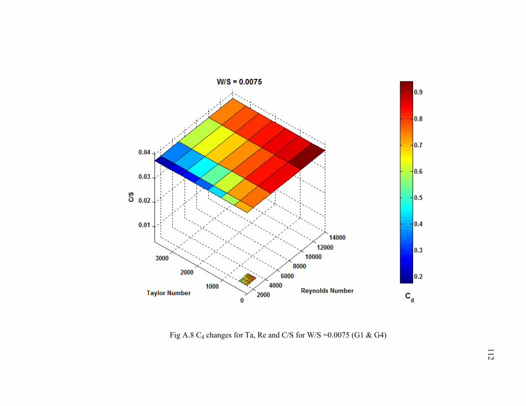
112
Fig A.8 Cd changes for Ta, Re and C/S for W/S =0.0075 (G1 & G4)
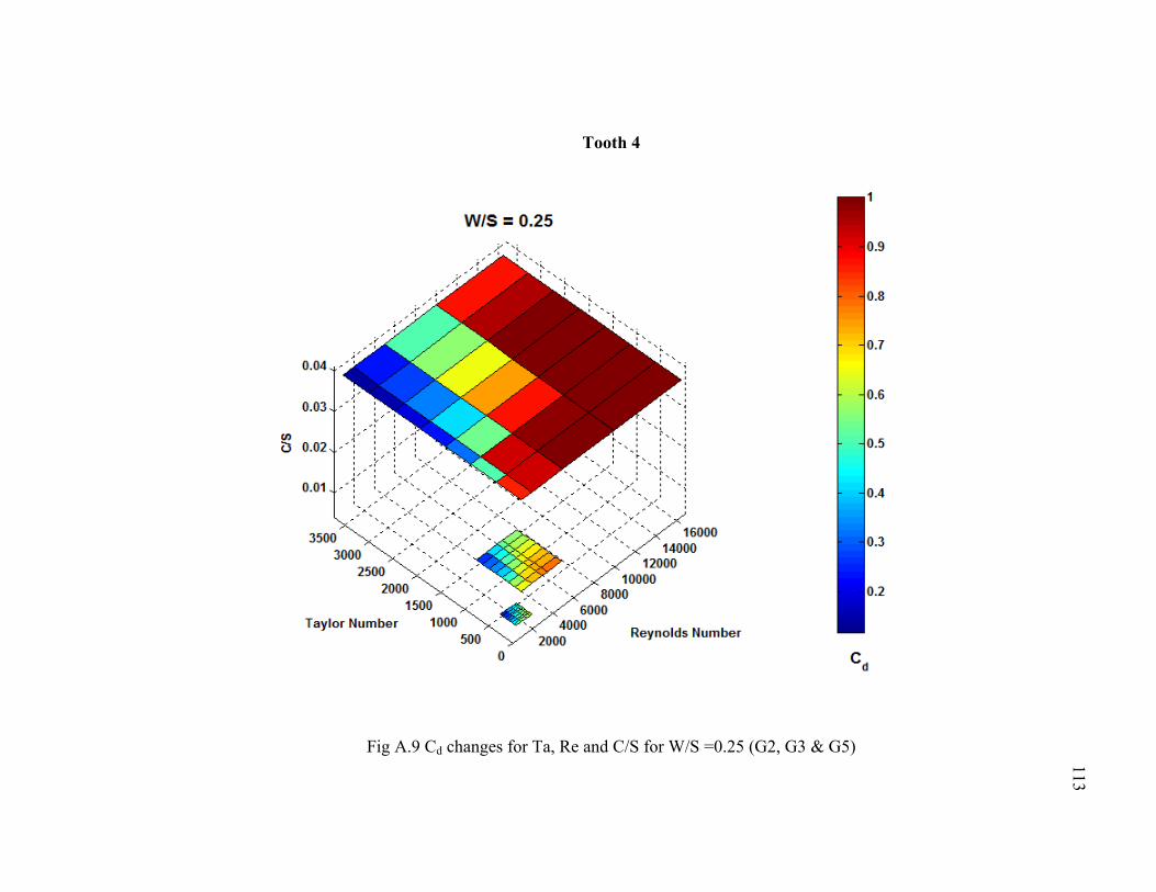
113
Tooth 4
Fig A.9 Cd changes for Ta, Re and C/S for W/S =0.25 (G2, G3 & G5)
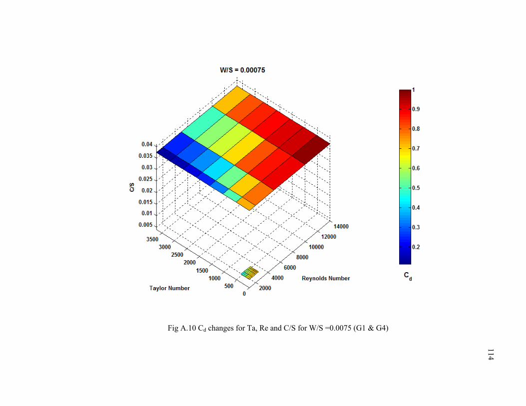
114
Fig A.10 Cd changes for Ta, Re and C/S for W/S =0.0075 (G1 & G4)
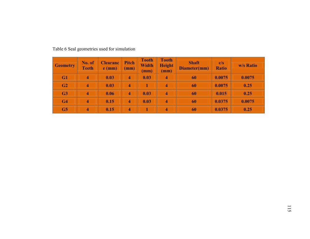
115
Table 6 Seal geometries used for simulation
Geometry No. of
Teeth
Clearanc
e (mm)
Pitch
(mm)
Tooth
Width
(mm)
Tooth
Height
(mm)
Shaft
Diameter(mm)
c/s
Ratio w/s Ratio
G1 4 0.03 4 0.03 4 60 0.0075 0.0075
G2 4 0.03 4 1 4 60 0.0075 0.25
G3 4 0.06 4 0.03 4 60 0.015 0.25
G4 4 0.15 4 0.03 4 60 0.0375 0.0075
G5 4 0.15 4 1 4 60 0.0375 0.25
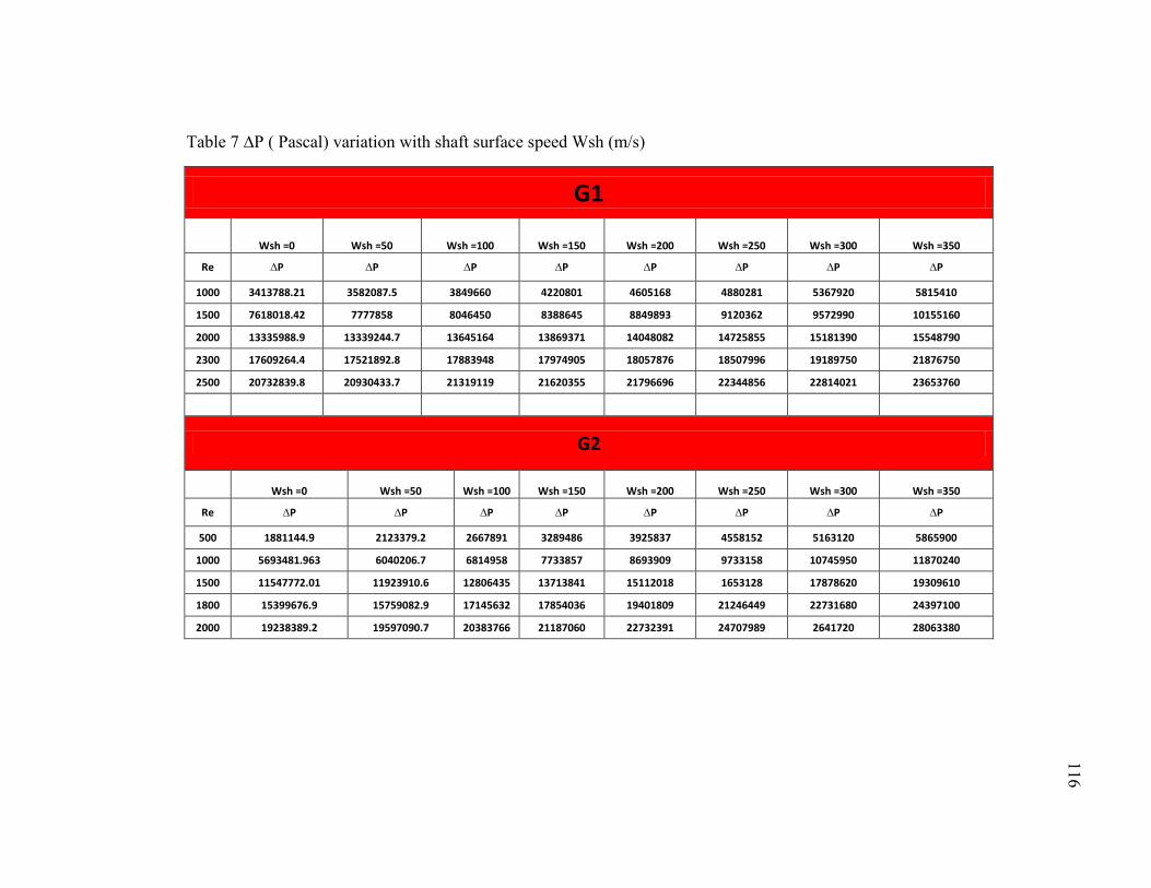
116
Table 7 ∆P ( Pascal) variation with shaft surface speed Wsh (m/s)
G1
Wsh =0 Wsh =50 Wsh =100 Wsh =150 Wsh =200 Wsh =250 Wsh =300 Wsh =350
Re ∆P ∆P ∆P ∆P ∆P ∆P ∆P ∆P
1000 3413788.21 3582087.5 3849660 4220801 4605168 4880281 5367920 5815410
1500 7618018.42 7777858 8046450 8388645 8849893 9120362 9572990 10155160
2000 13335988.9 13339244.7 13645164 13869371 14048082 14725855 15181390 15548790
2300 17609264.4 17521892.8 17883948 17974905 18057876 18507996 19189750 21876750
2500 20732839.8 20930433.7 21319119 21620355 21796696 22344856 22814021 23653760
G2
Wsh =0 Wsh =50 Wsh =100 Wsh =150 Wsh =200 Wsh =250 Wsh =300 Wsh =350
Re ∆P ∆P ∆P ∆P ∆P ∆P ∆P ∆P
500 1881144.9 2123379.2 2667891 3289486 3925837 4558152 5163120 5865900
1000 5693481.963 6040206.7 6814958 7733857 8693909 9733158 10745950 11870240
1500 11547772.01 11923910.6 12806435 13713841 15112018 1653128 17878620 19309610
1800 15399676.9 15759082.9 17145632 17854036 19401809 21246449 22731680 24397100
2000 19238389.2 19597090.7 20383766 21187060 22732391 24707989 2641720 28063380
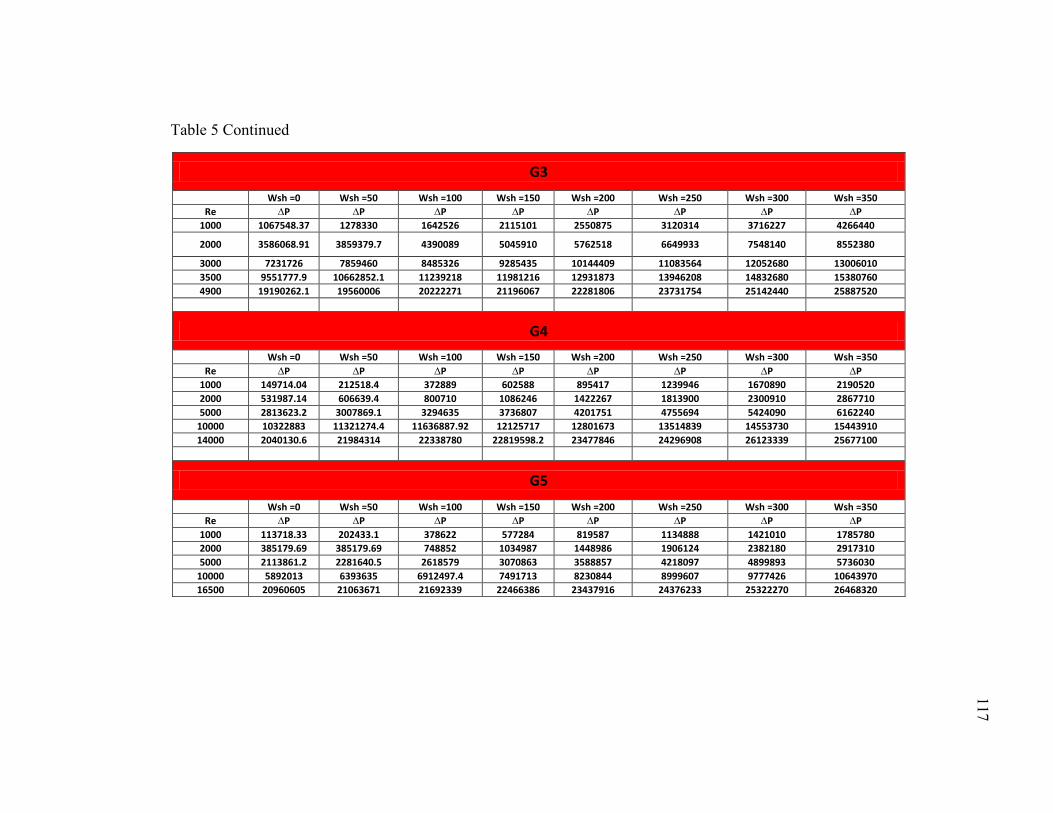
117
Table 5 Continued
G3
Wsh =0 Wsh =50 Wsh =100 Wsh =150 Wsh =200 Wsh =250 Wsh =300 Wsh =350
Re ∆P ∆P ∆P ∆P ∆P ∆P ∆P ∆P
1000 1067548.37 1278330 1642526 2115101 2550875 3120314 3716227 4266440
2000 3586068.91 3859379.7 4390089 5045910 5762518 6649933 7548140 8552380
3000 7231726 7859460 8485326 9285435 10144409 11083564 12052680 13006010
3500 9551777.9 10662852.1 11239218 11981216 12931873 13946208 14832680 15380760
4900 19190262.1 19560006 20222271 21196067 22281806 23731754 25142440 25887520
G4
Wsh =0 Wsh =50 Wsh =100 Wsh =150 Wsh =200 Wsh =250 Wsh =300 Wsh =350
Re ∆P ∆P ∆P ∆P ∆P ∆P ∆P ∆P
1000 149714.04 212518.4 372889 602588 895417 1239946 1670890 2190520
2000 531987.14 606639.4 800710 1086246 1422267 1813900 2300910 2867710
5000 2813623.2 3007869.1 3294635 3736807 4201751 4755694 5424090 6162240
10000 10322883 11321274.4 11636887.92 12125717 12801673 13514839 14553730 15443910
14000 2040130.6 21984314 22338780 22819598.2 23477846 24296908 26123339 25677100
G5
Wsh =0 Wsh =50 Wsh =100 Wsh =150 Wsh =200 Wsh =250 Wsh =300 Wsh =350
Re ∆P ∆P ∆P ∆P ∆P ∆P ∆P ∆P
1000 113718.33 202433.1 378622 577284 819587 1134888 1421010 1785780
2000 385179.69 385179.69 748852 1034987 1448986 1906124 2382180 2917310
5000 2113861.2 2281640.5 2618579 3070863 3588857 4218097 4899893 5736030
10000 5892013 6393635 6912497.4 7491713 8230844 8999607 9777426 10643970
16500 20960605 21063671 21692339 22466386 23437916 24376233 25322270 26468320
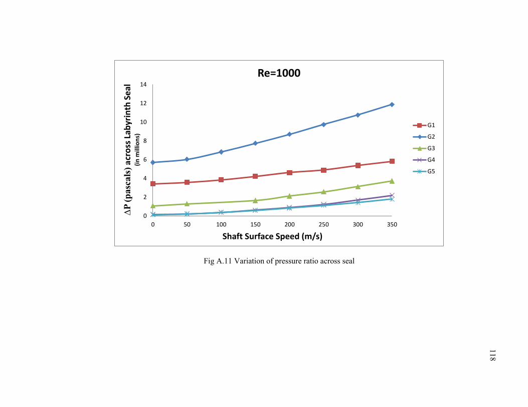
118
Fig A.11 Variation of pressure ratio across seal
0
2
4
6
8
10
12
14
0 50 100 150 200 250 300 350
∆P
(p
asc
als
) a
cro
ss L
abyr
inth
Se
al
(in
mill
ion
s)
Shaft Surface Speed (m/s)
Re=1000
G1
G2
G3
G4
G5
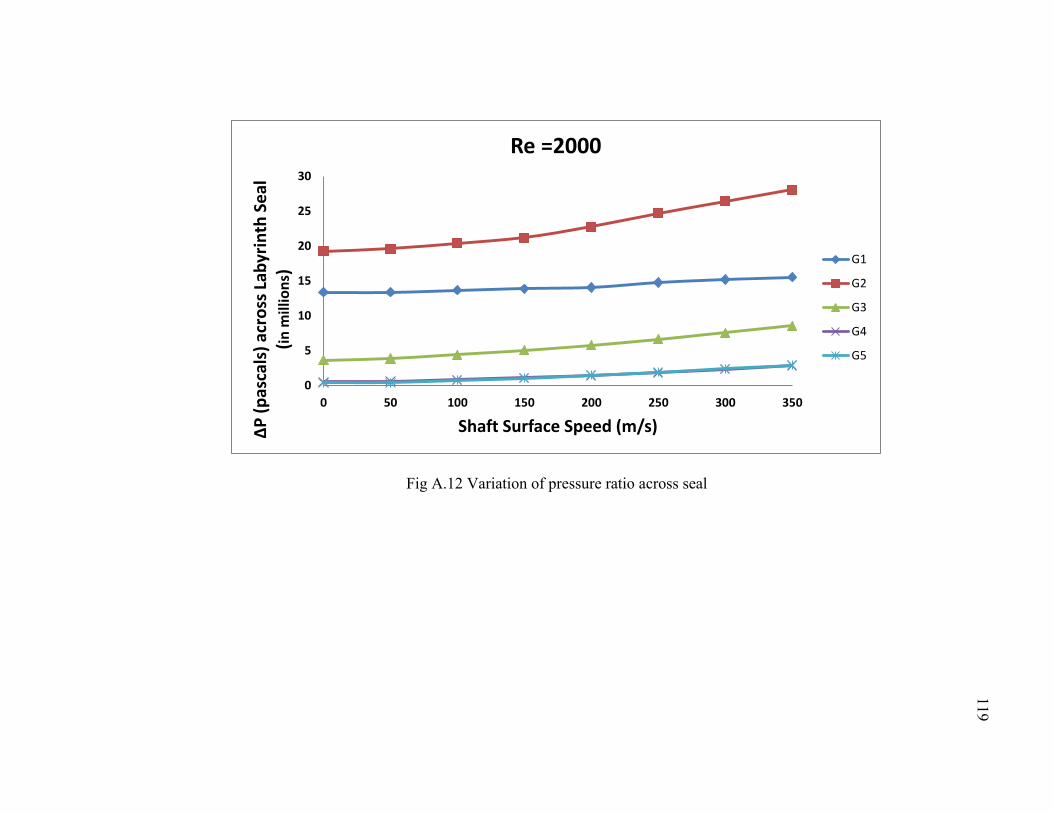
119
Fig A.12 Variation of pressure ratio across seal
0
5
10
15
20
25
30
0 50 100 150 200 250 300 350
∆P
(p
asca
ls)
acro
ss L
abyr
inth
Se
al
(in
mill
ion
s)
Shaft Surface Speed (m/s)
Re =2000
G1
G2
G3
G4
G5

120
Fig A.13 Large teeth geometry
Fig A.14 Small teeth geometry
121
The above Figure (A.13 & A.14) shows the variation pressure ratios across
different geometries for same Reynolds number/ mass flow rate. We could conclude
from the Figure 12.1 that seals with small clearances and larger tooth width (G2) are
performing better than the seals with lesser clearance and lower tooth width (G1).
Further to notify from Geometries G4 & G5 (same clearance different tooth width) we
note that the effect of tooth width is diminishing with increasing clearance where
throttling process is not so effective. Figure 12.2 also shows the same result with more
diminishing effect of tooth width with Reynolds number increasing where the pressure
difference is coinciding each other. Another aspect to be noted is that pressure difference
is increasing with shaft speed and the slope of increment does not matter change much
with increasing shaft surface speed.
122
VITA
Gaurav Chaudhary was born in Chitorgarh, India. He completed his high school
at BVB‟s Vidyasharm School, Jaipur, India. In 2004 he entered Panjab University,
Chandigarh, India. There, he completed his Bachelor Degree in mechanical engineering
with Honors in 2008. In August he entered the graduate school at Texas A&M
University and graduated August 2011.
Gaurav Chaudhary may be contacted through Texas A&M University‟s
Department of Mechanical Engineering at the following address:
Texas A&M University
Department of Mechanical Engineering
C/O Dr. Gerald Morrison
3123 TAMU
College Station, TX 77843 – 3123
USA.
Email address: [email protected]