
INVESTIGATION OF FIREFLY ALGORITHM AND CHAOS FIREFLY...
68
INVESTIGATION OF FIREFLY ALGORITHM AND CHAOS FIREFLY ALGORITHM FOR LOAD FREQUENCY CONTROL ZAID BIN NAJID FACULTY OF ENGINEERING UNIVERSITY OF MALAYA KUALA LUMPUR 2015
Transcript of INVESTIGATION OF FIREFLY ALGORITHM AND CHAOS FIREFLY...
INVESTIGATION OF FIREFLY ALGORITHM
AND CHAOS FIREFLY ALGORITHM FOR LOAD
FREQUENCY CONTROL
ZAID BIN NAJID
FACULTY OF ENGINEERING
UNIVERSITY OF MALAYA
KUALA LUMPUR
2015

INVESTIGATION OF FIREFLY ALGORITHM AND CHAOS FIREFLY
ALGORITHM FOR LOAD FREQUENCY CONTROL
ZAID BIN NAJID
RESEARCH REPORT SUBMITTED IN PARTIAL FULFILLMENT OF THE
REQUIREMENTS FOR THE DEGREE OF MASTER OF ENGINEERING
FACULTY OF ENGINEERING
UNIVERSITY OF MALAYA
KUALA LUMPUR
2015

UNIVERSITI MALAYA
ORIGINAL LITERARY WORK DECLARATION
Name of Candidate: ZAID BIN NAJID
Registration/Matric No : KMA110003
Name of Degree : Master of Engineering (Power System)
Title Research Report (“this
Work”)
: INVESTIGATION OF FIREFLY
ALGORITM AND CHAOS FIREFLY
ALGORITHM FOR LOAD FREQUENCY
CONTROL
Field of Study : Power System
I do solemnly and sincerely declare that:
(1) I am the sole author/writer of this Work;
(2) This Work is original;
(3) Any use of any work in which copyright exists was done by way of fair
dealing and for permitted purposes and any excerpt or extract from, or
reference to or reproduction of any copyright work has been disclosed
expressly and sufficiently and the title of the work and its authorship have
been acknowledged in this Work;
(4) I do not have any actual knowledge nor do I ought reasonably to know that
the making of this work constitutes an infringement of any copyright work;
(5) I hereby assign all and every rights in the copyright to this Work to the
University of Malaya (“UM”), who henceforth shall be owner of the
copyright in this Work and that any reproduction or use in any form or by
any means whatsoever is prohibited without the written consent of UM
having been first had and obtained;
(6) I am fully aware that if in the course of making this Work I have infringed
any copyright whether intentionally or otherwise, I may be subject to legal
action or any other action as may be determined by UM.
……………………………………………
Candidate’s Signature Date:……………..
Subscribed and solemnly declared before,
……………………………………………
Witness’s Signature Date:……………..
Name:…………………………………….
Designation:……………………………...

i
ABSTRACT
The changes of the structure of the power system, size, and complexity have increased
the important of LFC. For this reason, this research studies the controller aspect of LFC
by using the Fractional Order Integral-Derivative (FOID) controller or IλD
µ Controller.
In order to obtain the best controller parameter values for LFC, Firefly Algorithm (FA)
and Chaos Firefly Algorithm (CFA) are used. This project analyzes the performance of
the algorithms based LFC in three power system area. The primary objectives of LFC
are to maintain frequency and minimize power interchanges with neighboring control
areas. These objectives are met by measuring a control error signal called the area
control error (ACE), which calculates the real power difference between generation and
load. In this project, the integral of time multiply squared error (ITSE) as the objective
function is used on the ACE. The model of the system is designed using Matlab
software to carry out simulation studies. Step input load deviation is injected to the
system at designated location and the optimization of ramp rate, speed regulation and
the IλD
µ parameters are carried out. The frequency deviation and tie line power changes
characteristics are analyzed to observe the system performance. The maximum
overshoot, settling time and ITSE value is also recorded and compared. Result shows
that the CFA is the best optimization method due to its robustness and consistency. The
project can be further improved by tuning the controller using other optimization
techniques and including other physical constraints.

ii
ABSTRAK
Perubahan stuktur pada sistem kuasa elektrik, saiz, dan kerumitanya meninggikan lagi
keperluan untuk menaik taraf LFC. Oleh sebab itu, laporan ini menyiasat perbezaan
antara teknik pampasan yang digunapakai iaitu algoritma api-api (FA) dan algoritma
“Chaos” FA (CFA) meggunakan “Fractional Order Integral-Derivative” (FOID) atau
IλD
µ di dalam LFC untuk mendapatkan parameter yang optimum. Projek ini
menganalisa prestasi algoritma-algoritma tersebut yang digunapakai di dalam LFC
untuk sistem kuasa tiga kawasan kawalan. Objektif utama LFC adalah untuk
mengekalkan frekuensi dan mengurangkan pertukaran kuasa dengan kawasan kawalan
yang bersebelahan. Objektif utama ini dapat dicapai dengan mengukur isyarat ralat
kawalan ataupun dipanggil Ralat Kawasan Kawalan (ACE), yang mengira perbezaan
kuasa sebenar antara penjanaan dan beban. Di dalam projek ini, “Integral Time
weighted Squared Error (ITSE)” yang dilaksanakan di dalam ACE. Model bayangan
menyerupai yang sebenar dibina menggunakan perisian Matalab untuk mensimulasi
system tersebut. Input “step” beban sisihan disuntik kepada tempat-tempat terpilih
dengan pengoptimuman parameter “ramp rate, speed regulation dan IλD
µ. Kemudian
tindak balas lajakan frekuensi dan perubahan kuasa pada pusat talian dianalisis. Nilai
lonjakan maksima, masa selesai dan ITSE direkodkan dan dibandingkan. Keputusan
menunjukkan CFA cara pengoptimuman yang terbaik kerana kestabilannya dan
kekonsistansinya. Projek ini dapat ditambah baik dengan meggunakan cara
pengoptimuman yang lain dan menambah kekangan fizikal yang lain.

iii
ACKNOWLEDGEMENTS
In the name of Allah, The Most Gracious, Most Merciful and Him alone worthy of all
praises.
First and foremost, I would like to express my gratitude to my supervisor, Assoc. Prof.
Dr. Hazlie bin Mokhlis for his knowledge, time, guidance and support in guiding me to
complete this research report. Appreciation is also extended to Mr. Kanendra, Mr.
Nazmi Zulkifli and Department of Electrical Engineering, Faculty Engineering for their
advice and support in completing this research report.
Thanks also to my parents ‘Mek’ and ‘Ayah’ and my family whom being so supportive
throughout my postgraduate studies and completing this research report. May Allah
reward them the best of gift. Not to be forgotten, I would like to thank my lovely wife
Murni for her support and patience for me. To my daughter, ‘Atikah, you are my
inspiration.
Last but not least, many thanks to those who have directly or indirectly have helped me
throughout completing this course. Your kindness and consideration are greatly
appreciated.

iv
TABLE OF CONTENTS
ABSTRACT i
ABSTRAK ii
ACKNOWLEDGEMENTS iii
TABLE OF CONTENTS iv
LIST OF FIGURES vii
LIST OF TABLES viii
LIST OF SYMBOLS AND ABBREVIATIONS ix
1.0 INTRODUCTION 1
1.1 Overview 1
1.2 Problem Statement 2
1.3 Objectives of Research 2
1.4 Project Methodology 2
1.5 Research Report Organization 4
2.0 LITERATURE REVIEW 5
2.1 Background 5
2.2 Basic Generator Control Loop 5
2.3 Automatic Generation Control (AGC) 6
2.4 Load Frequency Control (LFC) 9
2.5 Area Control Area (ACE) 10
2.6 Load Frequency Control Technique 11
v
2.6.1 Classical Control Technique 11
2.6.2 Optimal Control 12
2.6.3 Adaptive and Self Tuning 12
2.6.4 Robust Control 13
2.6.5 Fractional Order of ID (IλD
µ) Controller 13
2.7 Self Computing / Artificial Intelligent Technique 15
2.7.1 Fuzzy Logic 15
2.7.2 Artificial Neural Network 16
2.7.3 Firefly Algorithm 16
3.0 METHODOLOGY 19
3.1 Background 19
3.2 LFC and AGC Modeling 19
3.3 Three Area System AGC 20
3.4 Modeling of ACE 21
3.5 Optimization of Firefly Algorithm 22
3.6 Optimization of Chaos Firefly Algorithm 24
4.0 RESULTS & DISCUSSION 25
4.1 Introduction 25
4.2 System Parameter 25
4.3 System Testing 26
4.4 Results and Discussion 27
4.4.1 Case 1 Simultaneous Loading in All Areas 27
4.4.2 Case 2 Different Load Demand Injected at Each Area 29

vi
4.4.3 Case 3 Optimization of Ramp Rate 31
4.4.4 Case 4 Optimization of Speed Regulation 34
4.4.5 Case 5 Optimization of Ramp Rate and Speed Regulation 37
4.4.6 Comparison for All Cases 39
5.0 CONCLUSION AND FUTURE WORKS 41
5.1 Conclusion 41
5.2 Further Work 42
REFERENCE 43
APPENDIX – MATHLAB CODE 47

vii
LIST OF FIGURES
Figure 1.1 General Overview of Project Block Diagram 3
Figure 2.1 Schematic diagram of LFC and AVR of a synchronous generator 6
Figure 2.2 Single Area Power System 8
Figure 2.3 Three Area Power System 8
Figure 2.4 Firefly Algorithm General Pseudo Code 16
Figure 3.1 Single Area Power System Model 19
Figure 3.2: Single Area Power System with Two Generators Model 20
Figure 3.3 Three Area Power System Model with Two Generators 21
Figure 3.4 Close Up ITSE Block Diagram 22
Figure 3.5 Flow Chart for FA 23
Figure 4.1 Frequency Deviation Step Response Comparison for Case 1 28
Figure 4.2: Tie line power changes for Case 1 28
Figure 4.3: Frequency Deviation Step Response Comparison for Case 2 30
Figure 4.4: Tie line power changes for Case 2 31
Figure 4.5: Frequency Deviation Step Response Comparison for Case 3 32
Figure 4.6: Tie line power changes for Case 3 33
Figure 4.7: Frequency Deviation Step Response Comparison for Case 4 35
Figure 4.8: Tie line power changes for Case 4 36
Figure 4.9: Frequency Deviation Step Response Comparison for Case 5 38
Figure 4.10: Tie line power changes for Case 5 38

viii
LIST OF TABLES
Table 4.1 System Parameters for Three Area Power System 25
Table 4.2 System Test Configuration 26
Table 4.3 System Performance for Case 1 27
Table 4.4 Optimal FOID parameters Case 1 29
Table 4.5 System Performance for Case 2 29
Table 4.6 Optimal FOID parameters for Case2 31
Table 4.7 System Performance for Case 3 32
Table 4.8 Optimal Ramp Rate and FOID parameters for Scenario 3 34
Table 4.9 System Performance for Case 4 34
Table 4.10 Optimal FOID parameters and Speed Regulation for Scenario 4 36
Table 4.11 System Performance for Case 5 37
Table 4:12 Optimal PID parameters and system performance for Scenario 5 39
Table 4.13 System Performance for All Cases 40

ix
LIST OF SYMBOLS AND ABBREVIATIONS
AC Alternating Current
ACE Area Control Error
AGC Automatic Generation Control
AVR Automatic Voltage Regulator
CFA Chaos Firefly Algorithm
FA Firefly Algorithm
FOID Fractional Order Integral-Derivative
FOPID Fractional Order Proportional-Integral-Derivative
ID Integral-Derivative
ITSE Integral of Time Multiply Squared Srror
kW kilo-Watts
LFC Load Frequency Control
PID Proportional Integral Derivative

1
CHAPTER 1
INTRODUCTION
1.1 Overview
A power system is a non-linear and large-scale multi input multi output
(MIMO) dynamic system with huge numbers of variable together with the protection
devices, control loops with different dynamic responses and characteristic. Multiple
numbers of generators will supply power into the interconnected system to be
transmitted which will then be distributed to loads. However a successful operation of
interconnected power system requires a balance of the total generation with the load
demand with its losses. At any given time, the power system is possible to experience
fault or sudden changes that may yield to undesirable effects.
In power system generation, it is important to consider the active and reactive
power load demand. The power system controller should effectively compensate the
load requirement as it is constantly changing. Two most important network parameters
which are the voltage and frequency should be maintained at its specified limits
because any deviation to both of it may compromise the system security and stability.
The changes in active power will affect the frequency while changes in the
reactive power will affect the voltage. Thus both voltage and frequency are controlled
separately. Load Frequency Control (LFC) is a mechanism to control frequency which
will be reflected to the active power. Meanwhile, Automatic Voltage Regulator (AVR)
is to control voltage and the reactive power.

2
1.2 Problem Statement
In the past, research work has been conducted which compares a new controller,
named fractional order controller, IλD
µ with classical integer order (IO) such as I, PI,
and PID controllers (Sanjoy Debbarma, Lalit Chandra Saikia, Nidul Sinha, 2013). The
obtained results shown that IλD
µ controller provide improved dynamic response and
outperform the classical IO controller. Thus for this research, IλD
µ controller is used.
However to obtain the optimum parameters for IλD
µ controller is more tedious and time
consuming because there are four parameters to be determined; I, D, λ and µ
(fractional gains). Due to this complexity, meta-heuristic methods called Firefly
Algorithm (FA) and Chaos Firefly Algorithm (CFA) are applied to get the optimum
combination of the IλD
µ controller gains, to be used for the LFC in the interconnected
reheat thermal power system.
1.3 Objectives of Research
The main objectives of this project are:
a) To model LFC for three area non-reheat thermal with multiple generator power
system using Simulink function in Mathlab simulation software.
b) To integrate Firefly Algorithm (FA) and Chaos Firefly Algorithm (CFA) in the
LFC model.
c) To compare the performance of FA and CFA in determining optimum
combination of the IλD
µ controller gains.
1.4 Project Methodology
In order to achieve the above-mentioned objectives, these steps will be carried out:
a) Review of LFC, Automatic Generation Control (AGC), IλD
µ controller and FA
optimization method.

3
b) From the review, suitable LFC and AGC model will be selected. For the
system controller, two optimization techniques will be selected namely FA and
Chaos Firefly Algorithm (CFA). Both FA based controller is investigated for
this project.
c) Modeling of a three area interconnected thermal power system with multiple
generators in LFC with AGC by using Simulink in Matlab.
d) Build the programming code for the proposed algorithm using Matlab.
e) Test proposed algorithm by a set of step input load injection at designated
location and optimization of some physical constraints.
Figure 1.1 : General Overview of Project Block Diagram
The general overview of the project block diagram is shown in Figure 1.1. Real
power demand as unit step function is the input of the system. The controller is a IλD
µ
controller utilizing FA based optimization technique. The controller will perform
calculation and compensate the plant in accordance to the error signal. The error signal
is the difference of input signal with respect to the feedback of the plant. The plant is
represented using transfer function which corresponds to the plant generation model
and the time constants of the generator. The output of the system is the frequency
deviation of the system. It also acts as the feedback of the system.

4
1.5 Research Report Organization
This research report is structured into five main chapters:
Chapter One includes the overview, problem statement, objective and research report
organization.
Chapter Two discusses the literature review regarding generator control loop as a
whole, LFC model, Automatic Generation Control (AGC), Feedback Control System
method, the optimization algorithm which consists of the firefly algorithm and the
fractional order controller.
Chapter Three discusses on the methodology of this research. LFC and AGC of three
area system are modeled in this section.
Chapter Four shows the results obtained from Matlab simulation using FA based
controller on LFC. All results are highlighted here.
Chapter Five covers the conclusion of this research and emphasizes the future work that
can be extended.

5
CHAPTER 2
LITERATURE REVIEW
2.1 Background
This research focuses on the investigation of FA based for LFC using IλD
µ
controller. A literature review regarding this topic had been performed and presented in
this chapter. All theoretical and conceptual frameworks are explained in this chapter to
ensure the understanding of this project aligns with the objectives. This chapter
describes the necessary models and algorithms used for the simulation.
2.2 Basic Generator Control Loop
Changes in real power affect mainly the system frequency while reactive power
is less sensitive to changes in frequency and is mainly dependent on changes in voltage
magnitude. Thus real power and reactive power are controlled separately. LFC controls
the real power and Automatic Voltage Regulator (AVR) regulates the reactive power
and voltage magnitude.
In any generation either an isolated or interconnected power system, LFC and
automatic voltage regulator (AVR) equipment are installed at each generator. The
schematic diagram of the LFC and AVR loops is represent in Figure 2.1. The controller
is set of particular operating condition that has input of small changes in load demand
to maintain the frequency and voltage magnitude within the specified limit. The
excitation system time constant is much smaller than the prime mover time constant
and its transient decay much faster and does not affect the LFC dynamic. Thus, the
cross coupling between the LFC and AVR loops is negligible. The load frequency and
excitation voltage control are also analyzed separately.

6
Figure 2.1: Schematic diagram of LFC and AVR of a synchronous generator (Hadi
Saadat, 2004)
From the figure, which is assumed to be a steam turbine, LFC controls the valve
opening which controls the steam amount. Then the steam will enter into the turbine to
rotate it. AVR controls the excitation system voltage of the generator by supplying DC
voltage to the rotor field winding.
2.3 Automatic Generation Control (AGC)
Generation scheduling and control is an important component of daily power
system operation. The overall objective of AGC is to control the electrical output of
generators while to regulate with the continuous changing load in an economical
manner. AGC is a program containing much of the associated function. Power system
Turbine G
AVR
Voltage sensor
Gen. Field
Steam
Valve Control
Mechanism
LFC Frequency
Sensor
Excitation System

7
operator or the dispatcher which buy power from Generation Company (GENCO) will
sell it to consumer whom will interact most of the time with AGC to monitor its result
and give input as to improvise current condition. In order to effectively maintain
generation control within the power system, the AGC scheme is guided by the Area
Control Error (ACE).
AGC can be defined as a system that represents the mechanism or the action
that is taken to ensure maximum economy and optimum power flow in an
interconnected power system network that comprises of generation, transmission and
distribution. The objectives of AGC (Thomas M. Athay 1987):
a) Matching total system generation to total system load
b) Regulating system electrical frequency error to zero
c) Distributing system generation among control areas so that net area tie flows
match net area tie flow scheduled
d) Distributing area generation among area generation sources so that area
operating cost are minimized
AGC as it known can be analyzed for a single area system or multi areas
system. The main objective of AGC in a single area system or an isolated system is to
restore the system frequency to the nominal value because there are no other areas for
power to flow. Figure 2.2 below shows the block diagram of an AGC for a single area
or an isolated power system.

8
Control Area 3
Figure 2.2: Single Area Power System
Figure 2.2 shows the basic diagram for an isolated system. The generator and the
system load are connected to a series of connection in which the speed regulator plays a
role in maintaining the system frequency.
While for multi area system AGC, the generators are closely looped or coupled
together. This group of generators needs to be synchronized or exhibit coherent
properties. This will enable the group generators to be termed or referred to as a control
area. Figure 2.3 shows the diagram of three area control system. The interconnected
system can contain two or more control areas.
Figure 2.3: Three Area Power System
Load
Load
Load
Control Area 1
Control Area 2

9
Each control area in Figure 2.3 shall capable of supplying to its own area at the
first place. Meanwhile, power flows between the control areas through the tie-lines.
This means, there is an effect to the entire system even there is changes at any point in
the system.
2.4 Load Frequency Control (LFC)
It is still a common practice throughout the world especially on developing
countries to practice monopoly in electricity business. It means generation,
transmission and distribution of electricity are under control of a single body or entity.
Thus, for an isolated power system, within monopoly strategy, imbalance of power and
changes in loads does not a serious issue. Hence, referring to Figure 2.1, LFC task is
limited to restore the system frequency to the specified nominal value. There are
following possible ways to share the change in the load to maintain frequency:
i. Either of generating units caters the change in load (Flat Frequency
Regulation).
ii. All units share the change in load (Parallel Frequency Regulation).
Within real system, generating units are large in numbers, with introduction of
some Independent Power Producers (IPP) into the system, loads are more diverse
through the transmitting lines and the system surely is more complex. In controlling
this issue, frequently used technique is to divide the whole system into some relative
controllable smaller systems which been called control areas or multi area control.
Therefore, LFC that located in each of the control area within this multi area control
need to regulate area frequency plus to control the supplementary power at scheduled
values.

10
On the other hand, for region that practices the electricity industry deregulation,
the operational of the power system structure itself do add the byzantine in controlling
it. Before that, deregulation of electricity industry is reducing direct government
involvement in, and to increase the economic efficiency through a change in the
electricity industry. Deregulation do divides generation, transmission and distribution
commonly called GENCO, TRANSCO and DISCO accordingly to end the monopoly
whilst increase competition and maximizing profit.
Through this deregulated regime, the operational of the LFC is different such as
Free LFC, Charged LFC, Bilateral LFC, Tender Market LFC, Auction Market LFC and
Real Time Balancing LFC. All these type of LFC operations in deregulated regime are
not been discussed here but it is to highlight the importance of performance of LFC.
2.5 Area Control Error (ACE)
The deviation of interchanged power flow and frequency in the multi area
system is the derivation from ACE. F. Daneshfar et al. (2009), ACE is determined from
main system parameters such as frequency deviation, power flow deviation and prime
mover control. Hence, ACE is a quantity that represents the power mismatch between
the generation and the load by taking into account the above mentioned system
parameters. Transient analysis of the system provides valuable information on the
stability of the system and the ACE has to be regulated to zero. But, to regulate ACE to
zero is tough because load is always fluctuating. Thus, tie-line power and frequency
shall always be maintained to its scheduled value. Formula for deviation of tie-line
power flow and the frequency deviation is obtained from below (M.R.I Sheikh et. Al.
2009):

11
(2.1)
- is the tie-line power flow
- is frequency bias factor of the area
- is frequency deviation
Frequency Bias Factor
The frequency bias factor of an area is given as:
(2.2)
- is the load damping constant which is the percentage change in
load
- is the governor speed regulation
2.6 LFC Control Techniques
2.6.1 Classical Control Technique
Classically, AGC frequency deviation is minimized using flywheel type of
governor of synchronous machine. But the LFC objective control is not achieved. Bode
and Nyquist are the pioneering control engineers whom established links between the
frequency response of a control system and its closed-loop transient performance in the
time domain. However the response resulted into relatively large overshoot and
transient frequency deviation. In addition, the settling time of the system frequency
deviation of comparatively long and is of the order of 10s to 20s (D.R. Chaudury,2005).
Based on P. Kundur (1994) most of conventional LFC uses proportional integral
controller. But the disadvantage is the integral gain limit the system performance.
Increasing the gain will cause large oscillations thus taking long time to settle and

12
create instability to the system. Hence desirable transient recovery and low overshoot in
the dynamic response of the overall system shall be compromised from the integral
gain setting. But then using this PI controller with the enlargement and improvement of
modern power system risking the system oscillation propagate into wider area that can
cause total black out. Therefore advanced control method were introduced in LFC such
as optimal control, adaptive control and robust control.
2.6.2 Optimal Control
Modern optimal control theory which is one of the LFC regulator design
techniques enable electric power engineers to design an optimal control system with
respect to given performance criterion. Optimal control theory does create a new
direction to solve large multivariable control problems in a simplified version. The state
variable representation of the model is been considered in optimal control. Elgerd and
Fosha who are the first addressed optimal control concept in LFC by using a state
variable model and regulator problem of optimal control theory to develop new
feedback control law for interconnected power system (Fosha and Olle, 1970).
2.6.3 Adaptive and Self-Tuning
The controller performance in a system may not be optimal as the operating
point of a power system will keep changing throughout the day. Better approach to
ensure the system performance at it optimum state is to track the operating point and
using the updated parameters to compute the control. Perfect model following condition
or explicit parameters identification are usually required by adaptive control. The
objective of the adaptive control is to make the process under control less sensitive to
changes in plant parameters and to un-modeled plant dynamics (H. Shayeghi et
al.,2009).

13
2.6.4 Robust Control
In any power system control area, the uncertainties and disturbances are
differing to one another. This is due to load variation, changing system parameters and
characteristics, modeling error and environmental conditions. As per explain, randomly
changes in load daily makes the operating points of the power system keep changing.
That is the reason an optimal LFC based on nominal system is not suitable for LFC and
may create inadequate to provide the desired system functioning. Hence later design of
LFC controllers is using robust approach with the objectives to design load frequency
controllers which guarantee robust stability and robust performance even though the
parameters change verily (Wang Y, Zhou R, Wen C, 1993). In addition, robust
approach design is capable to use the physical constraints of power system and
considering the system uncertainties for the synthesis procedure. Nevertheless, the
larger the model, the connection between subsystems will be uncertain, parameter
variation will be broader, and the organizational structure of power systems will be
elaborate bigger.
2.6.5 Fractional Order ID (IλD
µ) Controller
In total, there are numerous techniques available in LFC but varying of
parameters and rejection of disturbance always being the problem statement. Recently
development of LFC is going to the direction of the fractional order controller’s
formulation. Based on the literature review on hand, fractional order controller is
known to have an exceptional ability in handling varying parameters, in rejection of
disturbance, robust to high frequency noise and reducing steady state errors while
improving stability for nonlinear systems. All this characteristic of fractional order
controller makes it flexible and desirable for control strategy.

14
Before we proceed, the term ‘Fractional’ or ‘Fractional Order’ is inaccurate and
instead more accurate term is ‘non-integer-order’ since the order itself can be irrational.
The reason is fractional order calculus is like a derivative or integral but with non-
integer order. For example, the expressions of
are usually found. But for
fractional order, it can be any real number or it is a fractional of a derivative or integral
like
.
For a start, the commonly used definition for fractional differential-integral by
Reimann-Liouville (R-L) is explained.
The R-L definition for fractional derivative is given
(2.3)
- , n is an integer
- is the Euler’s gamma function.
The R-L definition for fractional integral is given
(2.4)
- is the fractional operator
The Laplace transformation of Riemann-Liouville definition for the fractional
derivative of equation (2.3) is given by
(2.5)
-
- is the normal Laplace transformation
15
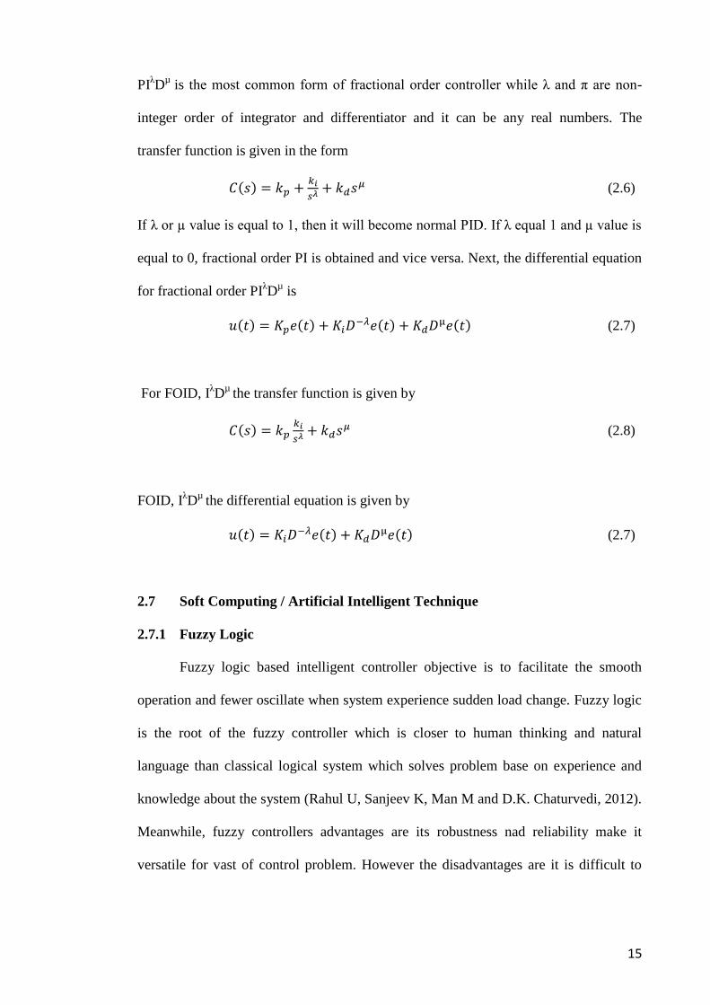
PIλD
µ is the most common form of fractional order controller while λ and π are non-
integer order of integrator and differentiator and it can be any real numbers. The
transfer function is given in the form
(2.6)
If λ or µ value is equal to 1, then it will become normal PID. If λ equal 1 and µ value is
equal to 0, fractional order PI is obtained and vice versa. Next, the differential equation
for fractional order PIλD
µ is
(2.7)
For FOID, IλD
µ the transfer function is given by
(2.8)
FOID, IλD
µ the differential equation is given by
(2.7)
2.7 Soft Computing / Artificial Intelligent Technique
2.7.1 Fuzzy Logic
Fuzzy logic based intelligent controller objective is to facilitate the smooth
operation and fewer oscillate when system experience sudden load change. Fuzzy logic
is the root of the fuzzy controller which is closer to human thinking and natural
language than classical logical system which solves problem base on experience and
knowledge about the system (Rahul U, Sanjeev K, Man M and D.K. Chaturvedi, 2012).
Meanwhile, fuzzy controllers advantages are its robustness nad reliability make it
versatile for vast of control problem. However the disadvantages are it is difficult to

16
acquire knowledge and there no adaptability and hence for dynamic time varying
system, it is unable to perform well due to change in system.
2.7.2 Artificial Neural Network (ANN)
ANN is unlike fuzzy controller. ANN does not require knowledge (Rule) but it
will find and identify patterns given appropriate design and training. ANN is like a
black box which compares non-linear connection between input and output. It is
inspired from our brain which contains hundreds of billions of neurons that connect
each other.
2.7.3 Firefly Algorithm
The Firefly Algorithm has been discovered by Xin-She Yang in 2007 which is
inspired from the firefly behavior.
Figure 2.4 : Firefly Algorithm General Pseudo Code

17
The main objective for a firefly to flash its light is to create a signal system to
draw other firefly. The FA is formulated by these three assumptions:
i. All fireflies are unisex, thus one firefly will be attracted by other firefly
ii. Attractiveness is proportional to their brightness, and for any two fireflies,
the less bright one will be attracted by and move closer to the brighter one;
however, the brightness can decrease as their distance increases;
iii. The firefly will move randomly if there are no fireflies brighter than a given
firefly.
In FA, there are two vital features to be considered:
i. the variation of light intensity.
ii. formulation of attractiveness.
The relationship between light intensity and distance denotes by:
(2.9)
where I is the intensity, is the original light intensity and is the light absorption
coefficient. For this research, the value of is 1.
If the light of a firefly is more intense, the brighter it is. Thus light density is
proportional to brightness. Brightness can be defines as
(2.10)
- is a constant that denote the present attractiveness at r=0
For this research, the value of is 0.2. The distance of any two fireflies i and j at xi
and xj, can be defined as the Cartesian distance
(2.11)

18
The movement of a firefly i is attracted towards more attractive (brighter) firefly j can
be calculated by
(2.12)
- is the randomization parameter
- is a vector of random numbers which drawn from Gaussian
distribution
(2.13)
From Equation 2.19, two limiting cases will occur which is γ small and large. When γ
is close to zero, a firefly can easily be seen by all other fireflies because the
attractiveness and brightness become constant. But when γ is very large, the
attractiveness (brightness) decreases dramatically, which maybe the environment the
fireflies fly are in thick foggy where they cannot see each other or maybe the fireflies
are short sighted; this means all fireflies move almost randomly, which corresponds to a
random search technique. Thus, the firefly algorithm correlates to the situation between
these two maximum.

19
CHAPTER 3
METHODOLOGY
3.1 Background
This chapter describes the methodology used in modeling the test system using
Mathlab software. The modeling of overall generation system and the parameter feed in
the model are explained. The method of the study was divided into four stages:
a. Study on knowledge related to LFC and AGC.
b. Model the system.
c. Capture all data required.
d. Analyze best data gathered.
3.2 LFC and AGC Modelling
Each LFC model consists of the generator model, load model, prime mover
model, governor model and physical constraints (time delay and dead band). All these
sub models is build and connected together to create the simulation block as shown in
Figure 3.1:
Figure 3.1 : Single Area Power System Model

20
Figure 3.1 shows a close loop of sinlge area LFC system. For generating the
most accurate model as compared to real, some physical constraints have been included
which are the time delay and ramping rate. In LFC system, any signal processing and
filtering introduces delays that should be considered. Typical filters on tie-line metering
and ACE signal (with the response characteristics of generator units) uses about 2
seconds or more for the data acquisition and decision cycles of the LFC systems.
However the introduction of this time delay will reduce the effectiveness of the LFC
performance.
For this project, two generators were included in each control area. Another one
set of generator model were inserted as per Figure 3.2 below.
Figure 3.2 : Single Area Power System Model with Two Generators
3.3 Three Area System AGC
Single area control block diagram then is combined to form three area power
system as shown in Figure 3.3. From this model, interconnected thermal power system
with multiple generators is analyzed and implemented.

21
Figure 3.3 : Three Area Power System Model with 2 Generators
3.4 Modelling of ACE
Integral Time Weighted Squared Error (ITSE) is used as the objective function
to calculate the system performance. The mathematical equation is as below.
(3.1)
Thus for this project, three area power system is used. Hence, sum operator is added
(3.2)
22
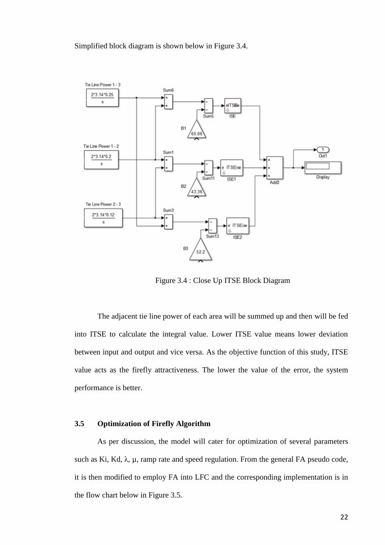
Simplified block diagram is shown below in Figure 3.4.
Figure 3.4 : Close Up ITSE Block Diagram
The adjacent tie line power of each area will be summed up and then will be fed
into ITSE to calculate the integral value. Lower ITSE value means lower deviation
between input and output and vice versa. As the objective function of this study, ITSE
value acts as the firefly attractiveness. The lower the value of the error, the system
performance is better.
3.5 Optimization of Firefly Algorithm
As per discussion, the model will cater for optimization of several parameters
such as Ki, Kd, λ, µ, ramp rate and speed regulation. From the general FA pseudo code,
it is then modified to employ FA into LFC and the corresponding implementation is in
the flow chart below in Figure 3.5.

23
Figure 3.5 : Flow Chart for FA
YES
NO
Start
Initialize and scale
Generate initial population of firefly
While
(k < Maximum Iteration)
for i = 1:no_of_fireflies
for j = 1:no_of_fireflies Calculate distance rij
Fireflies are ranked and the best solution
is updated, end while
End
Objective function of fireflies
is evaluated f(x) based on error
criterion
Light intensity Ii at xi is
determined based on f(xi)
Fireflies are ranked based on
their light intensity and the
best solution (firefly and its
light intensity) is stored
if (Ij > Ii)
Move firefly i towards j
Determine attractiveness β(r)
using chaos and movement of
fireflies end if
Evaluate new solutions and the
corresponding light intensity
end j, end i
YES
NO

24
3.6 Optimization of Chaos Firefly Algorithm
Chaos is introduced to existing FA by modifying the β. In this CFA algorithm,
Chebyshev map (A.H. Gandomi, 2012) is being investigated. The difference between
FA and CFA is the usage of Chebyshev map for movement of the new generated
firefly. The equation is shown below:
(3.3)
From the basic equation of FA
(3.4)
Hence, replacing Equation 3.3 into Equation 3.4 for the firefly attractiveness,
(3.4)
25
CHAPTER 4
RESULTS AND DISCUSSION
4.1 Background
After the firefly based algorithm had been integrated in the fractional order
controller for the three area power system using Simulink as per explained in previous
chapter, the results obtained will be presented and analyzed in this chapter. Both FA
and CFA had been tested and been compared.
The objective function of each case of the simulation is to get the lowest Area
Control Error. The fractional order controller parameters achieved to get the best result
are extracted as the output of the program.
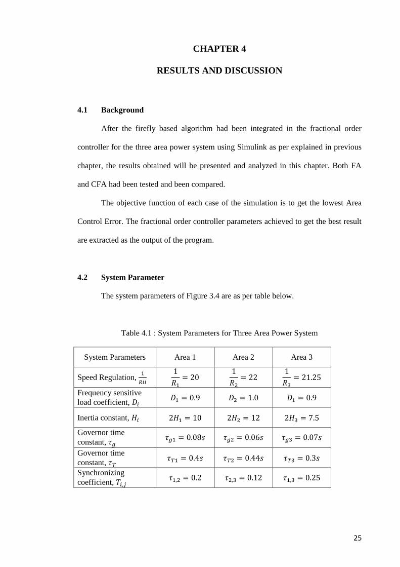
4.2 System Parameter
The system parameters of Figure 3.4 are as per table below.
Table 4.1 : System Parameters for Three Area Power System
System Parameters Area 1 Area 2 Area 3
Speed Regulation,
Frequency sensitive
load coefficient,
Inertia constant,
Governor time
constant,
Governor time
constant,
Synchronizing
coefficient,

26
4.3 System Testing
The system has been tested for five cases. Table 4.2 below describes the
configuration of each cases.
Table 4.2: System Test Configuration
Case Load Demand
Variation
Ramp Rate
Optimization
Speed Regulation
Optimization
1
∆PL1=0.1 p.u.
∆PL2=0.1 p.u.
∆PL3=0.1 p.u.
- -
2
∆PL1=0.3 p.u.
∆PL2=0.2 p.u.
∆PL3=0.1 p.u.
- -
3
∆PL1=0.1 p.u.
∆PL2=0.1 p.u.
∆PL3=0.1 p.u.
4
∆PL1=0.1 p.u.
∆PL2=0.1 p.u.
∆PL3=0.1 p.u..
-
5
∆PL1=0.1 p.u.
∆PL2=0.1 p.u.
∆PL3=0.1 p.u.
The first case has been conducted to test the system when all parameters are set
constant with the condition that nominal load demand of 0.1 p.u. had been injected at
each area. The second case has been conducted to analyze the performance of the
system when the simultaneously injected load demand is varied at each area. For the
third case, the system has been conducted to optimize the Ramp Rate gain while the
forth case has been tested to optimize the Speed Regulation gain. Lastly, the fifth case,
the system has been tested with both optimization of Ramp Rate and Speed Regulation.
The investigation of the system includes the following criteria:
i. Integral Time Weighted Squared Error, ITSE
ii. Settling Time (s) – Time required for the output to settle with respect to the
step input.

27
iii. Peak Frequency Overshoot (%) – The peak value of the frequency overshoot
value (in percentage) with respect to the nominal frequency.
4.4 Result and Discussion
4.4.1 Case 1 Simultaneous Loading in All Areas
Table 4.3 shows the result of the system performance when it is being tested for
the Case 1. The objective for this case is to investigate the performance of both FA and
CFA under all parameters are set constant.
Table 4.3: System Performance for Case 1
Method
Area 1 Area 2 Area 3
ITSE Settling
Time (s)
Peak
∆f
(Hz)
Settling
Time (s)
Peak
∆f
(Hz)
Settling
Time (s)
Peak
∆f
(Hz)
FA 13.7987 3.66% 16.5518 5.34% 14.5119 3.72% 0.2414
CFA 14.0805 3.91% 12.9642 4.71% 14.2734 4.76% 0.2411
Figure 4.1 shows the frequency deviation step response comparison for FA and CFA.
While Figure 4.2 shows tie line power changes.
(a) Frequency deviations in Area 1 (b) Frequency deviations in Area 2
0 5 10 15 20 25 30 35 40 45-4
-3.5
-3
-2.5
-2
-1.5
-1
-0.5
0
0.5
1x 10
-3
fre
q. d
ev
iati
on
(H
z)
time (sec)
FA
CFA
0 5 10 15 20 25 30 35 40 45-4
-3.5
-3
-2.5
-2
-1.5
-1
-0.5
0
0.5
1x 10
-3
fre
q. d
ev
iati
on
(H
z)
time (sec)
FA
CFA

28
(c) Frequency deviations in Area 3
Figure 4.1: Frequency Deviation Step Response Comparison for Case 1
(a) Tie line power changes in Area 1 (b)Tie line power changes in Area 2
(c) Tie line power changes in Area 3
Figure 4.2: Tie line power changes for Case 1
0 5 10 15 20 25 30 35 40 45-4
-3.5
-3
-2.5
-2
-1.5
-1
-0.5
0
0.5
1x 10
-3
fre
q. d
ev
iati
on
(H
z)
time (sec)
FA
CFA
0 10 20 30 40 50 60 70 80 90 100-2.5
-2
-1.5
-1
-0.5
0x 10
-3
tie
-lin
e p
ow
er
(p.u
.MW
)
time (sec)
FA
CFA
0 10 20 30 40 50 60 70 80 90 100-0.5
0
0.5
1
1.5
2
2.5
3x 10
-3
tie
-lin
e p
ow
er
(p.u
.MW
)
time (sec)
FA
CFA
0 10 20 30 40 50 60 70 80 90 100-12
-10
-8
-6
-4
-2
0
2
4
6x 10
-4
tie
-lin
e p
ow
er
(p.u
.MW
)
time (sec)
FA
CFA

29
A nominal load demand of 0.1 p.u. had been injected simultaneously for this
case at each area. For Area 1 and Area 3, CFA showed the highest frequency overshoot,
while for Area 2, the FA frequency overshoot is higher. However for settling time, for
Area 1 and Area 3, FA settled faster while for Area 2, CFA settled faster. From Figure
4.2, after 100 seconds, tie-line power of CFA is closer to zero for Area 1 and Area 3.
Comparing the ITSE value, CFA give better value than FA. Table 4.4 indicate the
optimal FOID parameters for Case 1.
Table 4.4: Optimal FOID parameters Case 1
FOID parameters
Method Area Ki Kd λ μ
Area 1 0.2415 0.1782 0.9800 0.0908
FA Area 2 0.4076 0.3325 0.9142 0.4031
Area 3 0.3144 0.0953 0.9002 0.3790
Area 1 0.2852 0.1356 0.9176 0.2988
CFA Area 2 0.3683 0.2786 0.9352 0.2617
Area 3 0.3234 0.1619 0.9127 0.3898
4.4.2 Case 2 Different Load Demand Injected at Each Area
For Case 2, the simultaneously load demand applied at Area 1, Area 2 and Area
3 are 0.3 p.u., 0.2 p.u. and 0.1 p.u. accordingly. Table 4.5 shows the result of the system
performance.
Table 4.5: System Performance for Case 2
Method
Area 1 Area 2 Area 3
ITSE Settling
Time (s)
Peak
∆f
(Hz)
Settling
Time (s)
Peak
∆f
(Hz)
Settling
Time (s)
Peak
∆f
(Hz)
FA 13.7271 1.79% 20.9272 1.24% 41.6626 6.82% 1.4147
CFA 11.9939 1.47% 16.4823 8.69% 38.9543 3.44% 1.3248
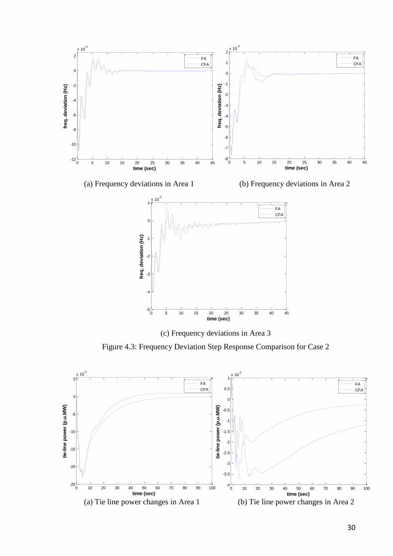
Figure 4.3 shows the frequency deviation step response comparison for FA and CFA
while Figure 4.4 shows tie line power changes.
30
(a) Frequency deviations in Area 1 (b) Frequency deviations in Area 2
(c) Frequency deviations in Area 3
Figure 4.3: Frequency Deviation Step Response Comparison for Case 2
(a) Tie line power changes in Area 1 (b) Tie line power changes in Area 2
0 5 10 15 20 25 30 35 40 45-5
-4
-3
-2
-1
0
1x 10
-3
fre
q. d
ev
iati
on
(H
z)
time (sec)
FA
CFA
0 5 10 15 20 25 30 35 40 45-12
-10
-8
-6
-4
-2
0
2
x 10-3
fre
q. d
ev
iati
on
(H
z)
time (sec)
FA
CFA
0 5 10 15 20 25 30 35 40 45-8
-7
-6
-5
-4
-3
-2
-1
0
1
2x 10
-3
fre
q. d
ev
iati
on
(H
z)
time (sec)
FA
CFA
0 10 20 30 40 50 60 70 80 90 100-25
-20
-15
-10
-5
0
5
x 10-3
tie
-lin
e p
ow
er
(p.u
.MW
)
time (sec)
FA
CFA
0 10 20 30 40 50 60 70 80 90 100-4
-3.5
-3
-2.5
-2
-1.5
-1
-0.5
0
0.5
1x 10
-3
tie
-lin
e p
ow
er
(p.u
.MW
)
time (sec)
FA
CFA

31
(c) Tie line power changes in Area 3
Figure 4.4: Tie line power changes for Case 2
For Area 1 and Area 3, FA illustrated higher frequency maximum overshoot,
while for Area 2, the CFA frequency overshoot is higher. However for settling time,
CFA settled faster at all three area. From Figure 4.4, tie-line power of CFA is closer to
zero for all three area. Comparing the ITSE value, CFA give better value than FA.
Table 4.6 indicate the optimal FOID parameters for Case 2.
Table 4.6 : Optimal FOID parameters for Case2
FOID parameters
Method Area Ki Kd λ μ
Area 1 0.3063 0.1485 0.8983 0.3946
FA Area 2 0.4890 0.1662 0.7866 0.6064
Area 3 0.5138 0.2029 0.7531 0.7360
Area 1 0.2742 0.1058 0.9266 0.1831
CFA Area 2 0.3628 0.1217 0.8983 0.3386
Area 3 0.3596 0.1758 0.8648 0.3529
4.4.3 Case 3 Optimization of Ramp Rate
For Case 3, the simultaneously load demand applied at all area is same which is
0.1 p.u. However for this case, the optimization is not only on the FOID parameters, but
also on the Ramp Rate gain. Table 4.7 shows the result of the system performance.
0 10 20 30 40 50 60 70 80 90 1000
0.005
0.01
0.015
0.02
0.025
tie
-lin
e p
ow
er
(p.u
.MW
)
time (sec)
FA
CFA

32
Table 4.7: System Performance for Case 3
Method
Area 1 Area 2 Area 3
ITSE Settling
Time (s)
Peak
∆f
(Hz)
Settling
Time (s)
Peak
∆f
(Hz)
Settling
Time (s)
Peak
∆f
(Hz)
FA 17.1185 4.34% 15.2491 4.18% 14.4002 5.38% 0.2646
CFA 15.6414 4.07% 15.1290 3.70% 14.1772 4.19% 0.2492
Figure 4.5 shows the frequency deviation step response comparison for FA and CFA.
While Figure 4.6 shows tie line power changes.
(a) Frequency deviations in Area 1 (b) Frequency deviations in Area 2
Frequency deviations in Area 3
Figure 4.5: Frequency Deviation Step Response Comparison for Case 3
0 5 10 15 20 25 30 35 40 45-4
-3.5
-3
-2.5
-2
-1.5
-1
-0.5
0
0.5
1x 10
-3
fre
q. d
ev
iati
on
(H
z)
time (sec)
FA
CFA
0 5 10 15 20 25 30 35 40 45-4
-3.5
-3
-2.5
-2
-1.5
-1
-0.5
0
0.5
x 10-3
fre
q. d
ev
iati
on
(H
z)
time (sec)
FA
CFA
0 5 10 15 20 25 30 35 40 45-4
-3.5
-3
-2.5
-2
-1.5
-1
-0.5
0
0.5
x 10-3
fre
q. d
ev
iati
on
(H
z)
time (sec)
FA
CFA

33
(a) Tie line power changes in Area 1 (b) Tie line power changes in Area 2
(c) Tie line power changes in Area 3
Figure 4.6: Tie line power changes for Case 3
FA display higher frequency maximum overshoot at all area. Hence CFA settled
faster at all area. From Figure 4.6, tie-line power of CFA is closer to zero for all three
area. However for this Case 3, the different between CFA and FA is significant.
Comparing the ITSE value, CFA give better value than FA. Table 4.8 indicates the
optimal FOID parameters and Ramp Rate for Case 3.
0 10 20 30 40 50 60 70 80 90 100-8
-6
-4
-2
0
2
4
6
8
10
12x 10
-4
tie
-lin
e p
ow
er
(p.u
.MW
)
time (sec)
FA
CFA
0 10 20 30 40 50 60 70 80 90 100-0.5
0
0.5
1
1.5
2
2.5x 10
-3ti
e-l
ine
po
we
r (p
.u.M
W)
time (sec)
FA
CFA
0 10 20 30 40 50 60 70 80 90 100-20
-15
-10
-5
0
5x 10
-4
tie
-lin
e p
ow
er
(p.u
.MW
)
time (sec)
FA
CFA
34
Table 4.8 : Optimal Ramp Rate and FOID parameters for Scenario 3
FOID parameters
Method Area Ki Kd λ μ αgen1 αgen2
Area 1 0.6712 0.3538 0.9139 0.4857 0.2480 0.1604
FA Area 2 0.7923 0.3361 0.8718 0.5459 0.3250 0.1857
Area 3 0.3369 0.1215 0.8963 0.2737 0.7109 0.3125
Area 1 0.2994 0.1481 0.9163 0.3531 0.5803 0.3737
CFA Area 2 0.4521 0.2070 0.8858 0.4903 0.3953 0.4580
Area 3 0.5144 0.2712 0.9419 0.1827 0.3683 0.2115
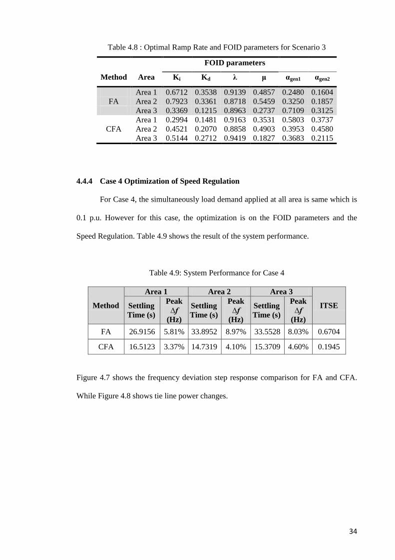
4.4.4 Case 4 Optimization of Speed Regulation
For Case 4, the simultaneously load demand applied at all area is same which is
0.1 p.u. However for this case, the optimization is on the FOID parameters and the
Speed Regulation. Table 4.9 shows the result of the system performance.
Table 4.9: System Performance for Case 4
Method
Area 1 Area 2 Area 3
ITSE Settling
Time (s)
Peak
∆f
(Hz)
Settling
Time (s)
Peak
∆f
(Hz)
Settling
Time (s)
Peak
∆f
(Hz)
FA 26.9156 5.81% 33.8952 8.97% 33.5528 8.03% 0.6704
CFA 16.5123 3.37% 14.7319 4.10% 15.3709 4.60% 0.1945
Figure 4.7 shows the frequency deviation step response comparison for FA and CFA.
While Figure 4.8 shows tie line power changes.

35
(a) Frequency deviations in Area 1 (b) Frequency deviations in Area 2
Frequency deviations in Area 3
Figure 4.7: Frequency Deviation Step Response Comparison for Case 4
(a) Tie line power changes in Area 1 (b) Tie line power changes in Area 2
0 5 10 15 20 25 30 35 40 45 50-5
-4
-3
-2
-1
0
1x 10
-3
fre
q. d
ev
iati
on
(H
z)
time (sec)
FA
CFA
0 5 10 15 20 25 30 35 40 45 50-5
-4
-3
-2
-1
0
1x 10
-3
fre
q. d
ev
iati
on
(H
z)
time (sec)
FA
CFA
0 5 10 15 20 25 30 35 40 45 50-5
-4
-3
-2
-1
0
1x 10
-3
fre
q. d
ev
iati
on
(H
z)
time (sec)
FA
CFA
0 10 20 30 40 50 60 70 80 90 100-2
-1
0
1
2
3
4
5
6
7x 10
-3
tie
-lin
e p
ow
er
(p.u
.MW
)
time (sec)
FA
CFA
0 10 20 30 40 50 60 70 80 90 100-2.5
-2
-1.5
-1
-0.5
0
0.5
1x 10
-3
tie
-lin
e p
ow
er
(p.u
.MW
)
time (sec)
FA
CFA
36
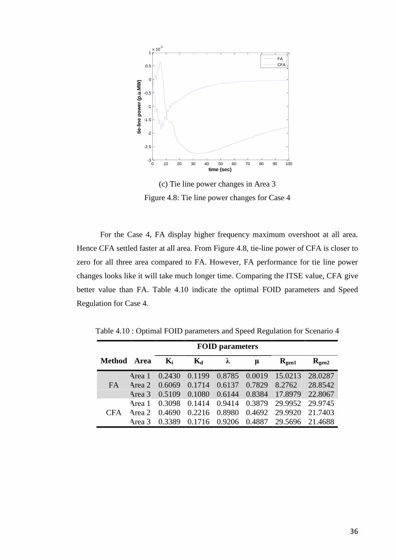
(c) Tie line power changes in Area 3
Figure 4.8: Tie line power changes for Case 4
For the Case 4, FA display higher frequency maximum overshoot at all area.
Hence CFA settled faster at all area. From Figure 4.8, tie-line power of CFA is closer to
zero for all three area compared to FA. However, FA performance for tie line power
changes looks like it will take much longer time. Comparing the ITSE value, CFA give
better value than FA. Table 4.10 indicate the optimal FOID parameters and Speed
Regulation for Case 4.
Table 4.10 : Optimal FOID parameters and Speed Regulation for Scenario 4
FOID parameters
Method Area Ki Kd λ μ Rgen1 Rgen2
Area 1 0.2430 0.1199 0.8785 0.0019 15.0213 28.0287
FA Area 2 0.6069 0.1714 0.6137 0.7829 8.2762 28.8542
Area 3 0.5109 0.1080 0.6144 0.8384 17.8979 22.8067
Area 1 0.3098 0.1414 0.9414 0.3879 29.9952 29.9745
CFA Area 2 0.4690 0.2216 0.8980 0.4692 29.9920 21.7403
Area 3 0.3389 0.1716 0.9206 0.4887 29.5696 21.4688
0 10 20 30 40 50 60 70 80 90 100-3
-2.5
-2
-1.5
-1
-0.5
0
0.5
1x 10
-3
tie
-lin
e p
ow
er
(p.u
.MW
)
time (sec)
FA
CFA

37
4.4.5 Case 5 Optimization of Ramp Rate and Speed Regulation
For Case 5, the simultaneously load demand applied at all area is same which is
0.1 p.u. However for this case, the optimization are on the FOID parameters, the Ramp
Rate and the Speed Regulation. Table 4.11 shows the result of the system performance.
Table 4.11: System Performance for Case 5
Method
Area 1 Area 2 Area 3
ITSE Settling
Time (s)
Peak
∆f
(Hz)
Settling
Time (s)
Peak
∆f
(Hz)
Settling
Time (s)
Peak
∆f
(Hz)
FA 20.8527 6.04% 16.1305 5.62% 14.4070 3.92% 0.2543
CFA 16.8636 3.42% 16.3315 3.92% 17.0528 4.57% 0.2306
Figure 4.9 shows the frequency deviation step response comparison for FA and CFA.
While Figure 4.10 shows tie line power changes.
(a) Frequency deviations in Area 1 (b) Frequency deviations in Area 2
0 5 10 15 20 25 30 35 40 45 50-4
-3.5
-3
-2.5
-2
-1.5
-1
-0.5
0
0.5
1x 10
-3
fre
q. d
ev
iati
on
(H
z)
time (sec)
FA
CFA
0 5 10 15 20 25 30 35 40 45 50-4
-3.5
-3
-2.5
-2
-1.5
-1
-0.5
0
0.5
1x 10
-3
fre
q. d
ev
iati
on
(H
z)
time (sec)
FA
CFA

38
Frequency deviations in Area 3
Figure 4.9: Frequency Deviation Step Response Comparison for Case 5
(a) Tie line power changes in Area 1 (b) Tie line power changes in Area 2
(c) Tie line power changes in Area 3
Figure 4.10: Tie line power changes for Case 5
0 5 10 15 20 25 30 35 40 45 50-4
-3.5
-3
-2.5
-2
-1.5
-1
-0.5
0
0.5
x 10-3
fre
q. d
ev
iati
on
(H
z)
time (sec)
FA
CFA
0 10 20 30 40 50 60 70 80 90 100-4
-3
-2
-1
0
1
2x 10
-3
tie
-lin
e p
ow
er
(p.u
.MW
)
time (sec)
FA
CFA
0 10 20 30 40 50 60 70 80 90 100-1
0
1
2
3
4
5
6x 10
-3
tie
-lin
e p
ow
er
(p.u
.MW
)
time (sec)
FA
CFA
0 10 20 30 40 50 60 70 80 90 100-3.5
-3
-2.5
-2
-1.5
-1
-0.5
0
0.5x 10
-3
tie
-lin
e p
ow
er
(p.u
.MW
)
time (sec)
FA
CFA

39
Finally, for Case 5, FA display higher frequency maximum overshoot at Area 1
and Area 2. At Area 3, CFA frequency overshoot is higher. For the settling time, at
Area 1 and Area 2, CFA settled faster while at Area 3, FA settled faster. From Figure
4.10, tie-line power of CFA is closer to zero for all three area compared to FA.
Comparing the ITSE value, CFA give better value than FA. Table 4.10 indicate the
optimal FOID parameters, Ramp Rate and Speed Regulation for Case 4.
Table 4:12 : Optimal FOID parameters and system performance for Scenario 5
FOID parameters
Method Area Ki Kd λ μ Rgen1 Rgen2 αgen1 αgen2
Area 1 0.5704 0.2217 0.8442 0.4030 25.4801 29.7432 0.3830 0.3029
FA Area 2 0.5397 0.2456 0.8399 0.8844 16.3297 27.1575 0.3891 0.4164
Area 3 0.4293 0.2966 0.9837 0.4079 28.2332 22.3602 0.1956 0.4397
Area 1 0.2897 0.1199 0.9036 0.5234 29.5721 24.8882 0.4659 0.5781
CFA Area 2 0.4859 0.2807 0.9003 0.5900 24.8167 22.3897 0.4747 0.3544
Area 3 0.8781 0.4418 0.9222 0.6481 20.8010 30.0000 0.2188 0.1485
4.4.5 Comparison of All Cases
Looking on overall for all cases, CFA give a smaller value for ITSE for all
cases. For Area 1, CFA frequency overshoot is lower at all cases except for Case 1. For
Area 2, CFA frequency overshoot is lower at all cases. For Area 3, CFA overshoot is
lower for Case 2, 3 and 4. For Area 1, the CFA settling time is shorter for all cases
except than Case 1. For Area 2, the CFA settling time is shorter for all cases except
than Case 5. For Area 3, CFA settling time is shorter for all cases except than Case 5
also. Table 4.13 below is detailed out the performance for every case.

40
Table 4:13: System Performance for All Cases
Case Method
Area 1 Area 2 Area 3
ITSE Settling
Time (s)
Peak ∆f
(Hz)
Settling
Time (s)
Peak ∆f
(Hz)
Settling
Time (s)
Peak ∆f
(Hz)
1
FA 13.7987 3.66% 16.5518 5.34% 14.5119 3.72% 0.2414
CFA 14.0805 3.91% 12.9642 4.71% 14.2734 4.76% 0.2411
2
FA 13.7271 1.79% 20.9272 1.24% 41.6626 6.82% 1.4147
CFA 11.9939 1.47% 16.4823 8.69% 38.9543 3.44% 1.3248
3
FA 17.1185 4.34% 15.2491 4.18% 14.4002 5.38% 0.2646
CFA 15.6414 4.07% 15.1290 3.70% 14.1772 4.19% 0.2492
4
FA 26.9156 5.81% 33.8952 8.97% 33.5528 8.03% 0.6704
CFA 16.5123 3.37% 14.7319 4.10% 15.3709 4.60% 0.1945
5
FA 20.8527 6.04% 16.1305 5.62% 14.4070 3.92% 0.2543
CFA 16.8636 3.42% 16.3315 3.92% 17.0528 4.57% 0.2306

41
CHAPTER 5
CONCLUSIONS AND FUTURE WORKS
5.1 Conclusion
Interconnected three area non-reheat thermal power system with multiple
generators of LFC has been modeled using Matlab Simulink. To achieve that, the sub-
systems such as the generator, governor, non-reheat steam turbine, load model and
physical constraint have been reviewed. Fractional Order Integral-Derivative (FOID) or
IλD
µ controller has been implemented into the LFC model. Fractional order concept has
been explained in Section 2.6.5. Self computing methods which include artificial
intelligent techniques have been looked into including the Firefly Algorithm which has
been chosen as the basis for the LFC optimization. In getting the optimum
configuration of IλD
µ controller, FA and CFA have been integrated into the LFC model.
Investigation of the performance of the CFA and FA based LFC controller have
been conducted. Simultaneous load demand has been injected at each area with
different value. Despite of the optimization on getting the optimum of IλD
µ controller
parameter, optimizations on the ramp rate and speed regulation gain have also been
conducted. ITSE has been selected as the objective function of this study which is used
as the performance indicator for the LFC.
From the result shown in Section 4.4, CFA based controller outperform FA
based controller in LFC non-reheat thermal power system with multiple generators.
CFA based controller shown lower ITSE value for the entire test and having better
settling time in most of the test. Tie-line power changes for CFA controller are all

42
settled to zero. All in all, both FA and CFA can be used as LFC controller optimization
method for IλD
µ controller with system remains stable.
5.2 Future Work
Some improvements can be done in order to achieve better performance LFC :
1. To include other physical constraints such as Governor Rate Constraints (GRC)
and uncertainties.
2. To investigate and apply IλD
µ controller into hyro-thermal generation model.
3. To increase the initial value of firefly and increase the iteration.
4. To vary the and value in the simulation.

43
REFERENCES
Bakken B. H., & Grande O. S. (November 1998). Automatic Generation Control in a
Deregulated Power System. IEEE Transactions on Power Systems, Vol. 13, No.
4, November 1998.
Cam E., & Kocaarsalan I. (2004). Load frequency control in two area power system
using fuzzy logic controller. Energy Conversion and Management 45 (2005)
233-243.
Chang C. S., & Fu W. (1998). Load frequency control using genetic-algorithm based
fuzzy gain scheduling of PI controllers. Electric Machines and Power System
Research (1998) 26:39-52.
Chang C. S., & Fu W. (1997). Area load frequency control using fuzzy gain scheduling
of PI controllers. Electric Power System Research 42 (1997). 145-152.
Concepcion Alicia Monje, YangQuan Chen, Blas Manueal Vinagre, Dingyu Xue,
Vicente Feliu. (2010). Fractional Order Systems and Controls. Springer
Demiroren, Zeynelgil H. L, & Sengor N. S. (September 2001). The Application of
ANN Technique to Load-frequency Control For Three-area Power System.
2001 IEEE Porto Power Tech Conference. 66
Dong L., Member, IEEE, & Zhang Y. (June 2010). On Design of a Robust Load
Frequency Controller for Interconnected Power Systems. American Control
Conference Marriott Waterfront, Baltimore, MD, USA

44
Douglas L. D., Green T. A., & Kramer R. A. (1993). New Approaches to the AGC
non- conforming load problem. IEEE Transaction on Power System.
Dy Liacco T. E. (1967). The Adaptive Reliability Control System. IEEE Transactions
On Power Apparatus And Systems Vol. Pas-86, No. 5 May 1967
F. Daneshfar, & H. Bevrani (2009). Load–frequency control: A GA-based multi-agent
reinforcement learning. IET Generation Transmission Distribution, 2010, Vol.
4, Iss. 1, pp. 13–26. doi: 10.1049/iet-gtd.2009.0168
Farahani S. M., Abshouri A. A., Nasiri B., & Meybodi M. R. (2011). A Gaussian
Firefly Algorithm. International Journal of Machine Learning and Computing,
Vol. 1, No. 5, December 2011. 67
Farook S., P. Sangameswara, Raju. (2012). Feasible AGC Controllers to Optimize LFC
Regulation in Deregulated Power System Using Evolutionary Hybrid Genetic
Firefly Algoroithm. J. Electrical System 8-4 (2012) 459-471
Farook S., & Sangameswara Raju P. (2012). Feasible AGC Controllers to Optimize
LFC Regulation in Deregulated Power System Using Evolutionary Hybrid
Genetic Firefly Algorithm. Regular paper - Journal of Electrical Systems 8-4
(2012): 459- 471.
Farahani M., Ganjefar S., & Alizadeh M. (2012). PID Controller Adjustment Using
Chaotic Optimization Algorithm For Multi-Area Load Frequency Control. IET
Control Theory and Applications (2012).

45
Gandomi A. H., Yang X. S., Talatahari S., & Alavi A. H. (2012). Firefly Algorithm
With Chaos. 2012 Elsevier Commun Nonlinear Sci Numer Simulat 18 (2013)
89–98.
H. Shayeghi, H.A. Shayanfar, A. Jalili. (Nov 2008). Load Frequency Control
Strategies: A State-of-the-Art Survey for the Researcher. Energy Conversion
and Management 50 (2009) 344-353
Hassan Bevrani (2009). Robust Power System Frequency Control, Springer.
Hadi Saadat (2004). Power System Analysis. McGraw-Hill, Inc.
Kanendra. N., Hazlie. M., & Abdul .Halim. A. B. (2013). Application Of Firefly
Algorithm (FA) Based Optimization In Load Frequency Control For
Interconnected Reheat Thermal Power System. 2013 IEEE Jordan Conference
on Applied Electrical Engineering and Computing Technologies (AEECT).
Kundur P. (1994). Power System Stability and Control. McGraw-Hill,Inc. 68
Lukasik S., & Zak S. (2009). Firefly Algorithm for Continuous Constrained
Optimization Tasks. Springer-Verlag Berlin Heidelberg 2009.
Sanjoy Debbarma, Lalit Chandra Saikia, Nidul Sinha. (Oct 2013). Solution to
Automatic Generation Control Prolem Using Firefly Algorith Optimized IλD
µ
Controller. ISA Transactions 53 (2014) 358-366

46
Sheikh M. R. I, Muyeen S. M., Member IEEE, Takahashi R., Member IEEE, Muraa T.,
& Tamura J., Senior Member IEEE (2009). Application of Self Tuning FPIC to
AGC for Load Frequency Control in Multi Area Power System. IEEE
Bucharest Power Tech Conference.
Sachin k. Jain, S. Chakrabarti, S. N. Singh. (2013). Review of Load Frequency Control
Methods. 2013 International Conference on COntrol, Automation, Robotics and
EMbedded Systems (CARE)
Shashi kant Pandeu, Soumya R. Mohanty, Nand Kishor. (Apr 2013). A Literature
Survey on Load-Frequency Control for Conventional and Distribution
Generation Power System. Renewable and Sustainable Energy Reviews 25
(2013) 318-334.
Swati Sondhi, Yogesh V. Hote. (June 2014). Fractional Order PID Controller for Load
Frequency Control. Energy Conversion and Management 85 (2014) 343-353
Thomas M. Athay. (Dec 1987). Generation Scheduling and Control. Proceedings of the
IEEE, VOl. 75, No. 12.
Yen J, Senior Member, IEEE (January/February 1999). Fuzzy Logic - A Modern
Perspective. IEEE Transactions On Knowledge And Data Engineering, Vol. 11,
No. [1]
Yang X. S. Firefly Algorithm, Stochastic Test Functions and Design Optimization.
Yang X. S (2010). Nature-Inspired Metaheuristic Algorithms. Luniver Press. 72

47
APPENDIX
MATHLAB CODE
FIREFLY ALGORITHM (FA)
%FireflyPID % clear all
no_fireflies = 20; MaxGeneration = 100; D=9; %/*The number of parameters of the problem to be
optimized*/ ub=1 ; %/*lower bounds of the parameters. */ lb=0.2; %/*upper bound of the parameters.*/ Range = ub-lb;
D2 = 6; ub2 = 1; lb2 = 0.001; Range2 = ub2-lb2;
% ------------------------------------------------
gamma=1.0; % Absorption coefficient delta=0.97; % Randomness reduction (similar to an annealing
schedule) alpha = 0.8; % Randomness 0--1 (highly random) betamin = 0.2;
% ------------------------------------------------
%Initialization runtime = 1;
runner = 1; for r=1:runtime
firefly = rand(no_fireflies,D) .* Range + lb; firefly2 = rand(no_fireflies,D2) .* Range2 + lb2; firefly = [firefly firefly2]; ObjVal = FFtracklsq89(firefly, no_fireflies)'; Fitness = calculateFitness(ObjVal);
for k=1:MaxGeneration %%%%% start iterations k
%------------------------------------------------- % This line of reducing alpha is optional % alpha=alpha_new(alpha,MaxGeneration); % alpha_n=alpha_0(1-delta)^NGen=10^(-4); % alpha_0=0.9
delta=1-(10^(-4)/0.9)^(1/MaxGeneration); alpha=(1-delta)*alpha;

48
%-------------------------------------------------
% Evaluate new solutions (for all n fireflies) for i=1:no_fireflies %ObjVal(i) = (firefly(i).^2+firefly(i)).*cos(firefly(i)); ObjVal(i) = FFtracklsq89(firefly(i,:), 1)'; Lightn(i)=ObjVal(i); end
% Ranking fireflies by their light intensity/objectives [Lightn,Index]=sort(ObjVal); ns_tmp=firefly; for i=1:no_fireflies firefly(i,:)=ns_tmp(Index(i),:); end
% Find the current best fireflyo=firefly; Lighto=Lightn; Firelfybest=firefly(1,:); Lightbest=Lightn(1);
% For output only fbest(k,:)=Lightbest;
% Scaling of the system scale = abs(ub - lb); scale2 = abs(ub2 - lb2);
fireflyc = firefly; firefly = firefly(:,1:9); fireflyo1 = firefly(:,1:9); % Updating fireflies for i=1:no_fireflies % The attractiveness parameter beta=exp(-gamma*r) for j=1:no_fireflies r=sqrt(sum((firefly(i,:)-firefly(j,:)).^2)); % Update moves if Lightn(i)>Lighto(j), % Brighter and more attractive beta0=1; beta=(beta0-betamin)*exp(-gamma*r.^2)+betamin; tmpf=alpha.*(rand(1,D)-0.5).*scale; firefly(i,:)=firefly(i,:).*(1-
beta)+fireflyo1(j,:).*beta+tmpf; end end % end for j end % end for i
firefly2 = fireflyc(:,10:15); fireflyo2 = fireflyc(:,10:15); for i=1:no_fireflies % The attractiveness parameter beta=exp(-gamma*r) for j=1:no_fireflies r=sqrt(sum((firefly2(i,:)-firefly2(j,:)).^2)); % Update moves if Lightn(i)>Lighto(j), % Brighter and more attractive beta0=1; beta=(beta0-betamin)*exp(-gamma*r.^2)+betamin; tmpf2=alpha.*(rand(1,D2)-0.5).*scale2;

49
firefly2(i,:)=firefly2(i,:).*(1-
beta)+fireflyo2(j,:).*beta+tmpf2; end end % end for j end % end for i
fireflyb = [firefly firefly2]; firefly = fireflyb;
%Limits
for i2=1:no_fireflies
if (firefly(i2,1)<lb) firefly(i2,1) = lb; end if (firefly(i2,2)<lb) firefly(i2,2) = lb; end if (firefly(i2,3)<lb) firefly(i2,3) = lb; end if (firefly(i2,4)<lb) firefly(i2,4) = lb; end if (firefly(i2,5)<lb) firefly(i2,5) = lb; end if (firefly(i2,6)<lb) firefly(i2,6) = lb; end if (firefly(i2,7)<lb) firefly(i2,7) = lb; end if (firefly(i2,8)<lb) firefly(i2,8) = lb; end if (firefly(i2,9)<lb) firefly(i2,9) = lb; end
if (firefly(i2,10)<lb2) firefly(i2,10) = lb2; end if (firefly(i2,11)<lb2) firefly(i2,11) = lb2; end if (firefly(i2,12)<lb2) firefly(i2,12) = lb2; end if (firefly(i2,13)<lb2) firefly(i2,13) = lb2; end if (firefly(i2,14)<lb2) firefly(i2,14) = lb2; end if (firefly(i2,15)<lb2) firefly(i2,15) = lb2;

50
end
if (firefly(i2,1)>ub) firefly(i2,1) = ub; end if (firefly(i2,2)>ub) firefly(i2,2) = ub; end if (firefly(i2,3)>ub) firefly(i2,3) = ub; end if (firefly(i2,4)>ub) firefly(i2,4) = ub; end if (firefly(i2,5)>ub) firefly(i2,5) = ub; end if (firefly(i2,6)>ub) firefly(i2,6) = ub; end if (firefly(i2,7)>ub) firefly(i2,7) = ub; end if (firefly(i2,8)>ub) firefly(i2,8) = ub; end if (firefly(i2,9)>ub) firefly(i2,9) = ub; end
if (firefly(i2,10)>ub2) firefly(i2,10) = ub2; end if (firefly(i2,11)>ub2) firefly(i2,11) = ub2; end if (firefly(i2,12)>ub2) firefly(i2,12) = ub2; end if (firefly(i2,13)>ub2) firefly(i2,13) = ub2; end if (firefly(i2,14)>ub2) firefly(i2,14) = ub2; end if (firefly(i2,15)>ub2) firefly(i2,15) = ub2; end
end
pp(k,:) = Lightbest; % cc(k,:) = firefly; % cc2(k,:) = firefly2; Lightbest end
GlobalParams = Firelfybest; GlobalMin = Lightbest; Kp = GlobalParams(:,1) Ki = Kp/GlobalParams(:,2)

51
Kd = Kp*GlobalParams(:,3)
Kp2 = GlobalParams(:,4) Ki2 = Kp2/GlobalParams(:,5) Kd2 = Kp2*GlobalParams(:,6)
Kp3 = GlobalParams(:,7) Ki3 = Kp3/GlobalParams(:,8) Kd3 = Kp3*GlobalParams(:,9)
lambda = GlobalParams(:,10) mu = GlobalParams(:,11)
lambda2 = GlobalParams(:,12) mu2 = GlobalParams(:,13)
lambda3 = GlobalParams(:,14) mu3 = GlobalParams(:,15)
list(runner,:) = [Kp Ki Kd Kp2 Ki2 Kd2 Kp3 Ki3 Kd3 lambda mu lambda2
mu2 lambda3 mu3 GlobalMin]
end lambda_a = lambda; mu_a = mu; sim('FOC8') sysval1 = stepinfo(b1.signals.values,b1.time); sysper1 = [sysval1.SettlingTime sysval1.SettlingMin
sysval1.SettlingMax] sysval2 = stepinfo(b2.signals.values,b2.time); sysper2 = [sysval2.SettlingTime sysval2.SettlingMin
sysval2.SettlingMax] sysval3 = stepinfo(b3.signals.values,b3.time); sysper3 = [sysval3.SettlingTime sysval3.SettlingMin
sysval3.SettlingMax]
pastez = [list; sysper1 sysper2 sysper3 zeros(1,7)]
ddd = polxxx

52
CHAOS FIREFLY ALGORITHM (CFA)
%FireflyPID clear all
no_fireflies = 40; MaxGeneration = 150; D=9; %/*The number of parameters of the problem to be
optimized*/ ub=1 ; %/*lower bounds of the parameters. */ lb=0.2; %/*upper bound of the parameters.*/ Range = ub-lb;
D2 = 6; ub2 = 1; lb2 = 0.001; Range2 = ub2-lb2;
% ------------------------------------------------
gamma=1.0; % Absorption coefficient delta=0.97; % Randomness reduction (similar to an annealing
schedule) alpha = 0.8; % Randomness 0--1 (highly random) betamin = 0.2;
% ------------------------------------------------
%Initialization runtime = 1;
runner = 1; for r=1:runtime
firefly = rand(no_fireflies,D) .* Range + lb; firefly2 = rand(no_fireflies,D2) .* Range2 + lb2; firefly = [firefly firefly2]; ObjVal = FFtracklsq89(firefly, no_fireflies)'; Fitness = calculateFitness(ObjVal);
for k=1:MaxGeneration %%%%% start iterations k
%------------------------------------------------- % This line of reducing alpha is optional % alpha=alpha_new(alpha,MaxGeneration); % alpha_n=alpha_0(1-delta)^NGen=10^(-4); % alpha_0=0.9
delta=1-(10^(-4)/0.9)^(1/MaxGeneration); alpha=(1-delta)*alpha;
%-------------------------------------------------
% Evaluate new solutions (for all n fireflies) for i=1:no_fireflies

53
%ObjVal(i) = (firefly(i).^2+firefly(i)).*cos(firefly(i)); ObjVal(i) = FFtracklsq89(firefly(i,:), 1)'; Lightn(i)=ObjVal(i); end
% Ranking fireflies by their light intensity/objectives [Lightn,Index]=sort(ObjVal); ns_tmp=firefly; for i=1:no_fireflies firefly(i,:)=ns_tmp(Index(i),:); end
% Find the current best fireflyo=firefly; Lighto=Lightn; Firelfybest=firefly(1,:); Lightbest=Lightn(1);
% For output only fbest(k,:)=Lightbest;
% Scaling of the system scale = abs(ub - lb); scale2 = abs(ub2 - lb2);
fireflyc = firefly; firefly = firefly(:,1:9); fireflyo1 = firefly(:,1:9); % Updating fireflies for i=1:no_fireflies % The attractiveness parameter beta=exp(-gamma*r) for j=1:no_fireflies r=sqrt(sum((firefly(i,:)-firefly(j,:)).^2)); % Update moves if Lightn(i)>Lighto(j), % Brighter and more attractive beta0=1;
tmpf=alpha.*(rand(1,D)-0.5).*scale;
beta = abs(cos(j*abs(acosd(firefly(j,:))))); firefly(i,:)=firefly(i,:).*(1-
beta)+fireflyo1(j,:).*beta+tmpf; end end % end for j end % end for i
firefly2 = fireflyc(:,10:15); fireflyo2 = fireflyc(:,10:15); for i=1:no_fireflies % The attractiveness parameter beta=exp(-gamma*r) for j=1:no_fireflies r=sqrt(sum((firefly2(i,:)-firefly2(j,:)).^2)); % Update moves if Lightn(i)>Lighto(j), % Brighter and more attractive beta0=1;
tmpf2=alpha.*(rand(1,D2)-0.5).*scale2; beta2 = abs(cos(j*abs(acosd(firefly2(j,:))))); firefly2(i,:)=firefly2(i,:).*(1-
beta2)+fireflyo2(j,:).*beta2+tmpf2; end

54
end % end for j end % end for i
fireflyb = [firefly firefly2]; firefly = fireflyb;
%Limits
for i2=1:no_fireflies
if (firefly(i2,1)<lb) firefly(i2,1) = lb; end if (firefly(i2,2)<lb) firefly(i2,2) = lb; end if (firefly(i2,3)<lb) firefly(i2,3) = lb; end if (firefly(i2,4)<lb) firefly(i2,4) = lb; end if (firefly(i2,5)<lb) firefly(i2,5) = lb; end if (firefly(i2,6)<lb) firefly(i2,6) = lb; end if (firefly(i2,7)<lb) firefly(i2,7) = lb; end if (firefly(i2,8)<lb) firefly(i2,8) = lb; end if (firefly(i2,9)<lb) firefly(i2,9) = lb; end
if (firefly(i2,10)<lb2) firefly(i2,10) = lb2; end if (firefly(i2,11)<lb2) firefly(i2,11) = lb2; end if (firefly(i2,12)<lb2) firefly(i2,12) = lb2; end if (firefly(i2,13)<lb2) firefly(i2,13) = lb2; end if (firefly(i2,14)<lb2) firefly(i2,14) = lb2; end if (firefly(i2,15)<lb2) firefly(i2,15) = lb2; end
55
if (firefly(i2,1)>ub) firefly(i2,1) = ub; end if (firefly(i2,2)>ub) firefly(i2,2) = ub; end if (firefly(i2,3)>ub) firefly(i2,3) = ub; end if (firefly(i2,4)>ub) firefly(i2,4) = ub; end if (firefly(i2,5)>ub) firefly(i2,5) = ub; end if (firefly(i2,6)>ub) firefly(i2,6) = ub; end if (firefly(i2,7)>ub) firefly(i2,7) = ub; end if (firefly(i2,8)>ub) firefly(i2,8) = ub; end if (firefly(i2,9)>ub) firefly(i2,9) = ub; end
if (firefly(i2,10)>ub2) firefly(i2,10) = ub2; end if (firefly(i2,11)>ub2) firefly(i2,11) = ub2; end if (firefly(i2,12)>ub2) firefly(i2,12) = ub2; end if (firefly(i2,13)>ub2) firefly(i2,13) = ub2; end if (firefly(i2,14)>ub2) firefly(i2,14) = ub2; end if (firefly(i2,15)>ub2) firefly(i2,15) = ub2; end
end
pp(k,:) = Lightbest; % cc(k,:) = firefly; % cc2(k,:) = firefly2; Lightbest end
GlobalParams = Firelfybest; GlobalMin = Lightbest; Kp = GlobalParams(:,1) Ki = Kp/GlobalParams(:,2)

56
Kd = Kp*GlobalParams(:,3)
Kp2 = GlobalParams(:,4) Ki2 = Kp2/GlobalParams(:,5) Kd2 = Kp2*GlobalParams(:,6)
Kp3 = GlobalParams(:,7) Ki3 = Kp3/GlobalParams(:,8) Kd3 = Kp3*GlobalParams(:,9)
lambda = GlobalParams(:,10) mu = GlobalParams(:,11)
lambda2 = GlobalParams(:,12) mu2 = GlobalParams(:,13)
lambda3 = GlobalParams(:,14) mu3 = GlobalParams(:,15)
list(runner,:) = [Kp Ki Kd Kp2 Ki2 Kd2 Kp3 Ki3 Kd3 lambda mu lambda2
mu2 lambda3 mu3 GlobalMin]
end lambda_a = lambda; mu_a = mu; sim('FOC8') sysval1 = stepinfo(b1.signals.values,b1.time); sysper1 = [sysval1.SettlingTime sysval1.SettlingMin
sysval1.SettlingMax] sysval2 = stepinfo(b2.signals.values,b2.time); sysper2 = [sysval2.SettlingTime sysval2.SettlingMin
sysval2.SettlingMax] sysval3 = stepinfo(b3.signals.values,b3.time); sysper3 = [sysval3.SettlingTime sysval3.SettlingMin
sysval3.SettlingMax]
pastez = [list; sysper1 sysper2 sysper3 zeros(1,7)]
ddd = polxxx