Gustavo da Silva Stefano - Colégio Catarinense
221
UNISINOS UNIVERSITY PRODUCTION AND SYSTEMS ENGINEERING GRADUATE PROGRAM MASTER OF SCIENCE DEGREE GUSTAVO DA SILVA STEFANO DOES THE THEORY OF CONSTRAINTS IN SUPPLY CHAIN MANAGEMENT REALLY MATTER? An Assessment of the Impacts of the TOC in the Redesign of a Supply Chain São Leopoldo 2020
Transcript of Gustavo da Silva Stefano - Colégio Catarinense
UNISINOS UNIVERSITY
PRODUCTION AND SYSTEMS ENGINEERING GRADUATE PROGRAM
MASTER OF SCIENCE DEGREE
GUSTAVO DA SILVA STEFANO
DOES THE THEORY OF CONSTRAINTS IN SUPPLY CHAIN MANAGEMENT
REALLY MATTER? An Assessment of the Impacts of the TOC in the Redesign
of a Supply Chain
São Leopoldo
2020
GUSTAVO DA SILVA STEFANO
DOES THE THEORY OF CONSTRAINTS IN SUPPLY CHAIN MANAGEMENT
REALLY MATTER? An Assessment of the Impacts of the TOC in the Redesign
of a Supply Chain
Dissertation presented to the UNISINOS University in partial fulfillment of the requirements for the Degree of Master of Science in Production and Systems Engineering
Advisor: Prof. Daniel Pacheco Lacerda, D. Sc.
Co-Advisor: Profa. Dra. Maria Isabel W. M. Morandi
São Leopoldo
2020
Catalogação na Publicação (CIP): Bibliotecário Alessandro Dietrich - CRB 10/2338
S816d Stefano, Gustavo da Silva. Does the theory of constraints in supply chain management really matter? An assessment of the impacts of the TOC in the redesign of a supply chain / by Gustavo da Silva Stefano. – 2020.
219 f. : il. ; 30 cm. Dissertation (master of science degree) — UNISINOS
University, Production and Systems Engineering Graduate Program, São Leopoldo, RS, 2020.
Advisor: Daniel Pacheco Lacerda, D. Sc. Co-Advisor: Dra. Maria Isabel W. M. Morandi.
1. Theory of constraints. 2. Supply chain management. 3. System dynamics modeling. 4. Causal impact. 5. Supply chain replenishment system. I. Título.
CDU: 658.5
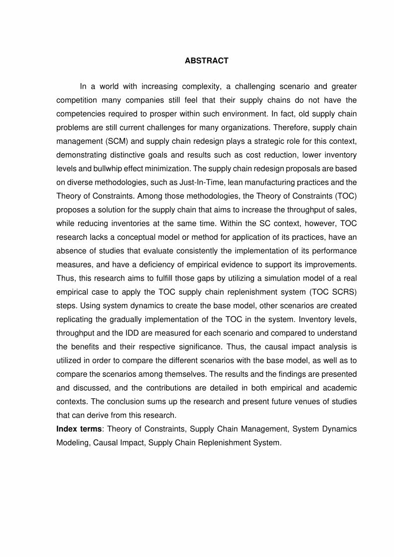
ABSTRACT
In a world with increasing complexity, a challenging scenario and greater
competition many companies still feel that their supply chains do not have the
competencies required to prosper within such environment. In fact, old supply chain
problems are still current challenges for many organizations. Therefore, supply chain
management (SCM) and supply chain redesign plays a strategic role for this context,
demonstrating distinctive goals and results such as cost reduction, lower inventory
levels and bullwhip effect minimization. The supply chain redesign proposals are based
on diverse methodologies, such as Just-In-Time, lean manufacturing practices and the
Theory of Constraints. Among those methodologies, the Theory of Constraints (TOC)
proposes a solution for the supply chain that aims to increase the throughput of sales,
while reducing inventories at the same time. Within the SC context, however, TOC
research lacks a conceptual model or method for application of its practices, have an
absence of studies that evaluate consistently the implementation of its performance
measures, and have a deficiency of empirical evidence to support its improvements.
Thus, this research aims to fulfill those gaps by utilizing a simulation model of a real
empirical case to apply the TOC supply chain replenishment system (TOC SCRS)
steps. Using system dynamics to create the base model, other scenarios are created
replicating the gradually implementation of the TOC in the system. Inventory levels,
throughput and the IDD are measured for each scenario and compared to understand
the benefits and their respective significance. Thus, the causal impact analysis is
utilized in order to compare the different scenarios with the base model, as well as to
compare the scenarios among themselves. The results and the findings are presented
and discussed, and the contributions are detailed in both empirical and academic
contexts. The conclusion sums up the research and present future venues of studies
that can derive from this research.
Index terms: Theory of Constraints, Supply Chain Management, System Dynamics
Modeling, Causal Impact, Supply Chain Replenishment System.
RESUMO
Em um mundo com uma complexidade crescente, um cenário desafiador e o
aumento da competitividade, muitas empresas sentem que suas cadeias de
suprimentos não possuem as competências necessárias para prosperar em tal
ambiente. Antigos problemas das cadeias de suprimentos, ainda, são desafios atuais
para em diversas organizações. Assim, a gestão da cadeia de suprimentos e o
redesenho dessas cadeias possuem um papel estratégico, demonstrando distintos
objetivos e resultados, tais como a redução de custos, menores níveis de inventário e
a redução do efeito chicote. As propostas de redesenho das cadeias se baseiam em
diversas metodologias, como o Just-In-Time, a produção enxuta e a Teoria das
Restrições (TOC). Dentre tais metodologias, a TOC propõe uma solução para a cadeia
que visa o aumento do ganho ao mesmo tempo que os estoques são reduzidos.
Dentro do contexto das cadeias de suprimentos, entretanto, as pesquisas de TOC
apresentam lacunas tais como: a falta de um modelo conceitual ou método para
aplicação de suas práticas; a falta de estudos que avaliem a implementação das suas
métricas de performance; e a deficiência de evidência empírica para suportar seus
benefícios. Assim, essa pesquisa objetiva sanar tais lacunas utilizando-se de uma
modelo de simulação baseado em um caso empírico real para aplicar a solução de
reabastecimento da cadeia de suprimentos da TOC. A modelagem de dinâmica de
sistemas é utilizada para a criação do modelo base e os outros cenários que simulam
a aplicação gradual de cada um dos passos da teoria. São mensurados os níveis de
inventário, o ganho, o inventário-dólar-dia (IDD) e a frequência de reabastecimento
são mensurados para cada cenário e comparados para melhor compreensão os
benefícios, assim como suas respectivas significâncias. A análise do impacto causal
é usada para comparar esses diferentes cenários com o modelo base, assim como
comparar os cenários entre si. Os resultados e as descobertas são apresentados e
discutidas, e as contribuições são detalhadas empiricamente e academicamente. A
conclusão resume a pesquisa e apresenta possíveis pesquisas futuras que podem
derivar do presente estudo.
Palavras-chave: Teoria das Restrições, Gestão da Cadeia de Suprimentos,
Modelagem de Dinâmica de Sistemas, Impacto Causal, Sistema de Reabastecimento
da Cadeia de Suprimentos.

LIST OF CHARTS
Chart 1 – Total number of publications by year ......................................................... 41
Chart 2 – Number of TOC and supply chain publications by journal ......................... 42
Chart 3 – Case’s consumption time series ................................................................ 72
LIST OF FIGURES
Figure 1 – Key enablers for SC operational improvements ....................................... 15
Figure 2 – Conflict between local and global optimum in the supply chain. ............... 19
Figure 3 – Mathematical effect of aggregation .......................................................... 20
Figure 4 – Selection method of the studies ............................................................... 27
Figure 5 – Schematic of the Theory of Constraints ................................................... 35
Figure 6 – The five-focusing steps and the continuous improvement process .......... 36
Figure 7 – TOC framework ........................................................................................ 38
Figure 8 – Thinking process application tools............................................................ 40
Figure 9 – TOC and SCM co-authorship network about TOC in SCM ...................... 44
Figure 10 – TOC in SCM co-authorship density map ................................................ 45
Figure 11 – Network of terms in TOC SC publications through time ......................... 47
Figure 12 – Aggregation at the PWH/CHW ............................................................... 57
Figure 13 – Replenishment schematic within the TOC supply chain ......................... 58
Figure 14 – Buffer penetration schematic for the supply chain .................................. 62
Figure 15 – Virtual buffer penetration example.......................................................... 64
Figure 16 – Pendulum for carrying out scientific research ......................................... 66
Figure 17 – Work methodology comparison .............................................................. 69
Figure 18 – Work Method .......................................................................................... 70
Figure 19 – Sales & Operations team and its connections ........................................ 73
Figure 20 – Forecast and planning cycle ................................................................... 74
Figure 21 – Rich picture of the analyzed supply chain. ............................................. 75
Figure 22 – Data analysis process flowchart ............................................................. 82
Figure 23 – Raw material forecast schematic............................................................ 87
Figure 24 – Internal supply chain for the RIG unit ..................................................... 94
Figure 25 – Basic supply chain model ....................................................................... 96
Figure 26 – Raw material exposure model representation ........................................ 99
Figure 27 – Re-ordering model representation ........................................................ 100
Figure 28 – Ordering raw material and seaport processing ..................................... 102
Figure 29 – Lead times module ............................................................................... 102
Figure 30 – Incoming purchases ............................................................................. 103
Figure 31 – Stock aggregation variable ................................................................... 104
Figure 32 – Internal supply chain with transfer orders ............................................. 105
6
Figure 33 – Buffer penetration modeling ................................................................. 107
Figure 34 – TOC planning module .......................................................................... 110
Figure 35 – Measures module ................................................................................. 112
Figure 36 – Base model and scenario 1 distributions comparison .......................... 126
Figure 37 – TDD causal impact plot between the base model and scenario 1 ........ 128
Figure 38 - Causal impact plot for IDD in scenario 1 ............................................... 130
Figure 39 – Causal impact plot for inventory in scenario 1 ...................................... 131
Figure 40 – Purchase frequency causal plot for scenario 1 ..................................... 133
Figure 41 - Base model and scenario 2 distributions comparison ........................... 137
Figure 42 – Causal impacts plots for scenario 2 ...................................................... 138
Figure 43 – Base model and scenario 3 distributions comparison .......................... 138
Figure 44 – Causal impacts plots for scenario 3 ...................................................... 139
Figure 45 – Base model and scenario 4 distributions comparison .......................... 140
Figure 46 – Causal impacts plots for scenario 4 ...................................................... 141
Figure 47 – Base model and scenario 5 distributions comparison .......................... 142
Figure 48 - Causal impacts plots for scenario 5 ...................................................... 143
Figure 49 – Base model and scenario 6 distributions comparison .......................... 144
Figure 50 – Causal impact plots for scenario 6 ....................................................... 145
Figure 51 – Scenarios 1 and 2 distributions comparison ......................................... 148
Figure 52 - Scenarios 2 and 3 distributions comparison .......................................... 149
Figure 53 – Scenarios 3 and 4 distributions comparison ......................................... 150
Figure 54 – Scenarios 4 and 5 distributions comparison ......................................... 151
Figure 55 - Scenarios 4 and 6 distributions comparison .......................................... 152
Figure 56 – Metrics module ..................................................................................... 182
Figure 57 – System Dynamics Model ...................................................................... 191
Figure 58 – Average total inventory confidence intervals ........................................ 192
Figure 59 – confidence invervals for KCL GR ......................................................... 192
Figure 60 – Confidence intervals for SAM GR......................................................... 193
Figure 61 – Confidence intervals for TSP GR ......................................................... 193
Figure 62 – Confidence intervals for UREIA GR ..................................................... 194
Figure 63 – Confidence intervals for YMILA 16 16 16 ............................................. 194
Figure 64 – Confidence intervals for YBELA AXAN ................................................ 195
Figure 65 – TDD impact for scenario 2 compared to the base model ..................... 196
Figure 66 – IDD impact for scenario 2 compared to the base model1 ..................... 196
7
Figure 67 – Total inventory impact for scenario 2 compared to the base model ..... 197
Figure 68 – Purchase frequency impact for scenario 2 compared to the base model
................................................................................................................................ 197
Figure 69 – TDD impact for scenario 3 compared to the base model ..................... 198
Figure 70 – IDD impact for scenario 3 compared to the base model ....................... 198
Figure 71 – Total inventory impact for scenario 3 compared to the base model ..... 199
Figure 72 – Purchase frequency impact for scenario 3 compared to the base model
................................................................................................................................ 199
Figure 73 – TDD impact for scenario 4 compared to the base model ..................... 200
Figure 74 – IDD impact for scenario 4 compared to the base model ....................... 200
Figure 75 – Total inventory impact for scenario 4 compared to the base model ..... 201
Figure 76 – Purchase frequency impact for scenario 4 compared to the base model
................................................................................................................................ 201
Figure 77 – TDD impact for scenario 5 compared to scenario the base model ....... 202
Figure 78 – IDD impact for scenario 5 compared to the base model ....................... 202
Figure 79 – Total inventory impact for scenario 5 compared to the base model ..... 203
Figure 80 – Purchase frequency impact for scenario 5 compared to the base model
................................................................................................................................ 203
Figure 81 – TDD impact for scenario 6 compared to scenario the base model ....... 204
Figure 82 – IDD impact for scenario 6 compared to scenario the base model ........ 204
Figure 83 – Total inventory impact for scenario 6 compared to the base model ..... 205
Figure 84 – Purchase frequency impact for scenario 6 compared to the base model
................................................................................................................................ 205
Figure 85 – TDD impact for scenario 2 compared to scenario 1 ............................. 206
Figure 86 – IDD impact for scenario 2 compared to scenario 1............................... 206
Figure 87 – Total inventory impact for scenario 2 compared to scenario 1 ............. 207
Figure 88 – Purchase frequency impact for scenario 2 compared to scenario 1 ..... 207
Figure 89 – TDD impact for scenario 3 compared to scenario 2 ............................. 208
Figure 90 – IDD impact for scenario 3 compared to scenario 2............................... 208
Figure 91 – Total inventory impact for scenario 3 compared to scenario 2 ............. 209
Figure 92 – Purchase frequency impact for scenario 3 compared to scenario 2 ..... 209
Figure 93 – TDD impact for scenario 4 compared to scenario 3 ............................. 210
Figure 94 – IDD impact for scenario 4 compared to scenario 3............................... 210
Figure 95 – Total inventory impact for scenario 4 compared to scenario 3 ............. 211
8
Figure 96 – Purchase frequency impact for scenario 4 compared to scenario 3 ..... 211
Figure 97 – TDD causal impact for scenario 5 compared to scenario 4 .................. 212
Figure 98 – IDD impact for scenario 5 compared to scenario 4............................... 212
Figure 99 – Total inventory impact for scenario 5 compared to scenario 4 ............. 213
Figure 100 – Purchase frequency impact for scenario 5 compared to scenario 4 ... 213
Figure 101 – TDD impact for scenario 6 compared to scenario 4 ........................... 214
Figure 102 – IDD impact for scenario 6 compared to scenario 4............................. 214
Figure 103 – Total inventory impact for scenario 6 compared to scenario 4 ........... 215
Figure 104 – Purchase frequency impact for scenario 6 compared to scenario 4 ... 215
LIST OF FRAMES
Frame 1 – Search of terms in the databases............................................................. 26
Frame 2 - TOC performance measures .................................................................... 37
Frame 3 – Content analysis categories ..................................................................... 48
Frame 4 – TOC supply chain / distribution solution steps ......................................... 49
Frame 5 – TOC SC concepts definitions ................................................................... 51
Frame 6 – Company’s specialists consulted ............................................................. 77
Frame 7 – Collected variables and sources .............................................................. 79
Frame 8 – Simulation scenarios and model variables ............................................... 84
Frame 9 – Raw material supply premise ................................................................... 89
Frame 10 – Comparison of the results .................................................................... 152
Frame 11 – TOC solution findings ........................................................................... 157
Frame 12 – Systematic review protocol .................................................................. 171
Frame 13 - Thesaurus of terms ............................................................................... 172
LIST OF TABLES
Table 1 – Improvements from TOC application ......................................................... 30
Table 2 – Yearly publications of TOC in supply chain by journal ............................... 43
Table 3 – Co-authorship clusters details ................................................................... 46
Table 4 – Document types and approaches .............................................................. 53
Table 5 – Studies’ type and approach distribution ..................................................... 54
Table 6 – Content analysis of TOC-SC solution steps .............................................. 55
Table 7 – Material origin premise and transit time ..................................................... 90
Table 8 – Port processing time .................................................................................. 91
Table 9 – Safety factor and batch premise ................................................................ 93
Table 10 – Inventory position (in thousand tons) for model verification ..................... 97
Table 11 – Forecast variable example ...................................................................... 98
Table 12 – Observations and purchase volumes by raw material ........................... 113
Table 13 – Model validation results ......................................................................... 114
Table 14 – Base model descriptive statistics ........................................................... 116
Table 15 – Shapiro-Wilk results for the results ........................................................ 116
Table 16 – Scenarios descriptive analysis for TDD and IDD ................................... 117
Table 17 – Scenarios descriptive analysis for inventory .......................................... 119
Table 18 – Descriptive analysis for purchase frequency ......................................... 120
Table 19 – Kruskal-Wallis test for the interest variables .......................................... 121
Table 20 – TDD multiple comparison test results .................................................... 121
Table 21 – IDD multiple comparison test results ..................................................... 122
Table 22 – Total inventory multiple comparison test results .................................... 123
Table 23 – Purchase frequency multiple comparison test results............................ 124
Table 24 – Causal impact results for TDD in scenario 1 ......................................... 129
Table 25 - Causal Impact results for IDD in scenario 1 ........................................... 130
Table 26 – Causal impact results for inventory in scenario 1 .................................. 132
Table 27 – Purchase frequency causal impact results in scenario 1 ....................... 133
Table 28 – Causal impact results ............................................................................ 135
Table 29 – Incremental causal impact ..................................................................... 147
Table 30 – Months and model time units ................................................................. 181
Table 31 – Schematic for time units and their relation with the forecast month ....... 183
Table 32 – Order probability distribution .................................................................. 186

11
Table 33 – Transit time probabilities ........................................................................ 187
Table 34 – Seaport processing probabilities ........................................................... 189
ACRONYMS LIST
CRT Current Reality Tree
DBM Dynamic Buffer Management
DBR Drum-Buffer-Rope
EC Evaporating Clouds
ECE Effect-Cause-Effect
FRT Future Reality Tree
I Investment
IDD Inventory-Dollar-Days
IT Information Technology
JIT Just-in-time
MRP Materials Resource Planning
OE Operational Expense
PRT Prerequisite Tree
SC Supply Chain
SCM Supply Chain Management
SD System Dynamics
S.D. Standard Deviation
SLR Systematic Literature Review
T Throughput
TDD Throughput-Dollar-Days
TOC Theory of Constraints
TOCRS Theory of Constraints Replenishment System
TT Transition Tree
INDEX
1 INTRODUCTION .................................................................................................... 15
1.1 RESEARCH AIM AND PROBLEM DEFINITION ................................................. 18
1.2 OBJECTIVES ...................................................................................................... 24
1.2.1 General Objective ........................................................................................... 24
1.2.2 Specific Objectives ........................................................................................ 25
1.3 JUSTIFICATION .................................................................................................. 25
1.4 DELIMITATIONS ................................................................................................. 32
1.5 WORK STRUCTURE .......................................................................................... 32
2 THEORETICAL BACKGROUND ........................................................................... 34
2.1 THEORY OF CONSTRAINTS ............................................................................. 34
2.2 TOC AND SUPPLY CHAIN MANAGEMENT ...................................................... 40
2.2.1 Descriptive Analysis ...................................................................................... 41
2.2.2 Content Analysis ............................................................................................ 47
3 METHODOLOGICAL PROCEDURES ................................................................... 66
3.1 RESEARCH METHODOLOGY ........................................................................... 66
3.2 WORK METHODOLOGY .................................................................................... 68
3.3 CASE OVERVIEW .............................................................................................. 71
3.4 DATA COLLECTION ........................................................................................... 76
3.5 DATA ANALYSIS ................................................................................................ 80
4 MODEL CONSTRUCTION ..................................................................................... 86
4.1 SYSTEM CONCEPTUALIZATION ...................................................................... 86
4.2 THE INTERNAL SUPPLY CHAIN MODULE ....................................................... 93
4.3 PLANNING AND REPLENISHMENT MODULE .................................................. 98
4.4 MODELING THE TOC STEPS .......................................................................... 104
4.4.1 Aggregating Stocks...................................................................................... 104
4.4.2 Determining Buffer Sizes Based on Demand, Supply, and The
Replenishment Lead ............................................................................................. 106
4.4.3 Managing Inventory Using Buffer Penetration .......................................... 107
4.4.4 Using Dynamic Buffers ................................................................................ 108
4.4.5 Creating a Hybrid Solution Utilizing Buffers and Forecast ....................... 109
4.4.6 Performance Measures ................................................................................ 111
4.5 MODEL VALIDATION ....................................................................................... 112
14
5 ANALYSIS OF THE RESULTS ........................................................................... 115
5.1 BASE MODEL RESULTS AND DESCRIPTIVE ANALYSIS .............................. 115
5.2 SCENARIO COMPARISON .............................................................................. 117
5.3 CAUSAL IMPACTS OF TOC STEPS APPLICATION ....................................... 124
5.3.1 Impacts with Regards to the Base Model ................................................... 125
5.3.2 Incremental Step Application Impacts Comparison .................................. 145
6 DISCUSSION OF THE RESULTS ....................................................................... 154
6.1 EMPIRICAL CONTRIBUTIONS WITHIN THE COMPANY CONTEXT.............. 154
6.2 ACADEMIC CONTRIBUTIONS ......................................................................... 156
7 CONCLUSION ..................................................................................................... 159
REFERENCES ........................................................................................................ 162
APPENDIX A – RESEARCH PROTOCOL ............................................................. 171
APPENDIX B – THESAURUS OF TERMS ............................................................. 172
APPENDIX C – MODEL TIME UNITS TABLE ....................................................... 181
APPENDIX D – METRICS MODULE ...................................................................... 182
APPENDIX E – FORECAST CALENDAR REPRESENTATION ............................ 183
APPENDIX F – ORDER TIME PROBABILITY FUNCTION .................................... 186
APPENDIX G – TRANSIT TIME PROBABILITY FUNCTION ................................. 187
APPENDIX H – SEAPORT PROCESSING PROBABILITY FUNCTION ................ 189
APPENDIX I – SYSTEM DYNAMICS MODEL OVERVIEW ................................... 191
APPENDIX J – CONFIDENCE INTERVALS OF RESULTS................................... 192
APPENDIX K – CAUSAL IMPACT PLOTS ............................................................ 196
APPENDIX L – CAUSAL IMPACT RESULTS ........................................................ 216
15
1 INTRODUCTION
A supply chain can be defined as a group of entities that manufacture, distribute
and/or sell goods within a flow created for an finished product that extends from its raw
materials up to the end customer delivery (BLACKSTONE, 2001). Supply chains are
integrated systems of ever-increasing complexity levels, therefore, innovative methods
for its integrated management are necessary (PONTE et al., 2016). Additionally, the
current challenges imposed by a global economy – such as rapid disruptive rates of
change and emergence of new innovative competitors – increase the need for effective
supply chain management (STEVENS; JOHNSON, 2016). The increased competition,
in this context, results in more customization possibilities to end customers, quality
improvements and greater demand responsiveness while at the same time aiming for
reduced production costs, lead-times and inventory levels, in order ensure profitability
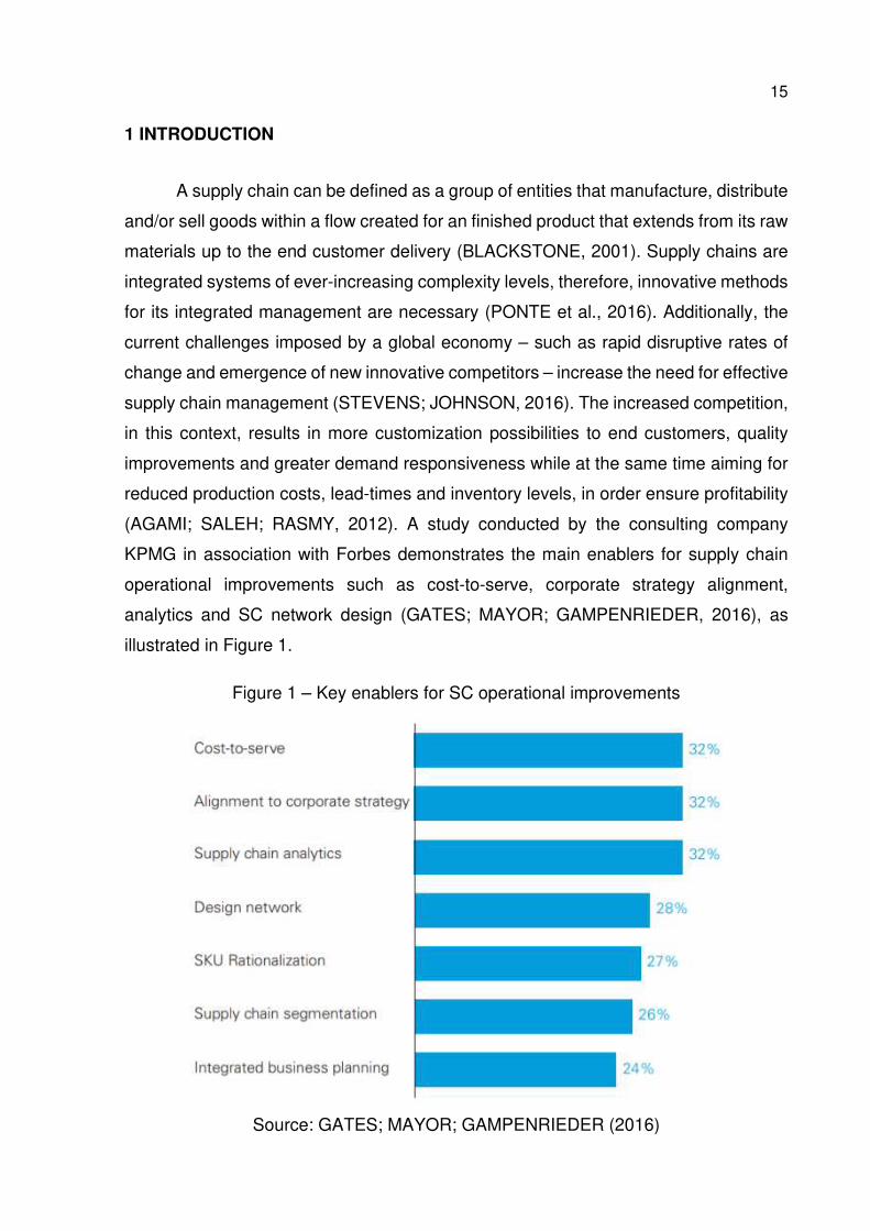
(AGAMI; SALEH; RASMY, 2012). A study conducted by the consulting company
KPMG in association with Forbes demonstrates the main enablers for supply chain
operational improvements such as cost-to-serve, corporate strategy alignment,
analytics and SC network design (GATES; MAYOR; GAMPENRIEDER, 2016), as
illustrated in Figure 1.
Figure 1 – Key enablers for SC operational improvements
Source: GATES; MAYOR; GAMPENRIEDER (2016)
16
With increasing complexity, a challenging scenario and greater competition
many companies feel that their supply chains do not have the competencies required
to prosper within this environment. In fact, old supply chain problems are still current
challenges for many companies. As demonstrated by a survey conducted in 17
different countries and 623 supply chain professionals, the top objectives of the supply
chains are to ensure deliveries on time and improve product availability or delivery
(GEODIS, 2017).
Within this context, supply chain redesign becomes a strategic decision for the
supply chain management (SCM) context (PIRARD; IASSINOVSKI; RIANE, 2008),
demonstrating distinctive goals and results such as cost reduction (MARTINS et al.,
2017), lower inventory levels (BERRY; NAIM, 1996) and bullwhip effect minimization
(NAIM; DISNEY; EVANS, 2002). The supply chain redesign proposals are based on
diverse methodologies, such as Just-In-Time (HUNT et al., 2009), lean manufacturing
practices (BUIL; PIERA; LASERNA, 2011) and the Theory of Constraints (WALKER,
2002). Among those methodologies, the Theory of Constraints (TOC) proposes a
solution for the supply chain that aims to increase the throughput of sales, while
reducing inventories at the same time. Basically, this is accomplished by aggregating
stocks at the SC highest point and utilizing buffers to manage the supply chain
replenishment (GUPTA; ANDERSEN, 2018; IKEZIRI et al., 2019). Thus, the TOC
practices pose as a interesting and beneficial topic of discussion for supply chain
management and consequently is defined as the subject of interest of this present
work.
According to Tulasi and Rao (2012), the TOC was derived from the OPT – a
system for production synchronization and planning – and has its origins in the ’70s,
just as the Just-In-Time (JIT) and the Material Resources Planning (MRP). The TOC
is a general approach for managing an organization (GOLDRATT, 1988). Rahman
(1998) claims that the TOC is based on two key points: a) every system has at least
one constraint; and b) the existence of a constraint represents an improvement
opportunity for the system. A constraint, as defined by Goldratt (1988), is anything that
limits a system from attaining its goal.
Basically, the TOC is composed of three main areas: logical thinking,
performance measurement, and logistics (TULASI; RAO, 2012). The logical thinking
aims at solving the problems of a system constraint through the application of the five-
17
step-focusing and the thinking process. According to Goldratt and Cox (2004), TOC’s
five focusing steps to ensure continuous improvement are:
a) Identify the system’s constraint;
b) Explore the constraint;
c) Subordinate the whole system to the constraint;
d) Elevate the constraint;
e) If the constraint is “broken” go back to the first step to avoid inertia stopping
the continuous improvement process.
Regarding its performance measures, the Theory of Constraints bases them on
the assumption that the goal of the organization is to make money now and in the
future (RAHMAN, 1998). Rahman (1998) explains that the TOC’s performance
measures can be separated in global measures and operational measures. According
to the author global measures include Net Profit (NP), Return Over Investment (ROI)
and Cash Flow (CF); operational measures are Throughput (T), Inventory (I) and
Operational Expenses (OE).
Related to logistics is the Drum-Buffer-Rope (DBR) method, which is a pull-
oriented strategy utilized to effectively manage the bottleneck of the system through
appropriate synchronization (PONTE et al., 2016; PUCHE et al., 2016). The drum is
the constraint or bottleneck, the component with the least capacity that limits the
throughput of the whole system (WATSON; POLITO, 2003). The rope acts like a
signaling mechanism that ties the constraint to material release (BLACKSTONE,
2001). Lastly, the buffer is a stock of materials that protect the constraint from the rest
of the system (BLACKSTONE, 2001)
Being initially applied in production planning, TOC has had its application
extended to many other areas such as performance measurement, marketing, sales
and supply chain management (BLACKSTONE, 2001). In the supply chain context,
the Theory of Constraints challenges the premise that the best way to manage a
distribution system is to refill inventory based on sales forecasting (BERNARDI DE
SOUZA; PIRES, 2010). The TOC supply chain solution aims to solve common
problems as low inventory turnovers, high investment on stocks, lack of finished
products that cause missing sales and inventory excess at the same time, stock
obsolescence and many others (SCHRAGENHEIM, 2010). According to
Scharagenheim (2010), the TOC solution purpose is to answer what, where and when
18
to stock, based upon the frequent replenishment of the consumed inventories through
strategically placed buffers.
The benefits of implementing TOC’s distribution system in the supply chain are
demonstrated equally through the theory’s performance measures and other more
commonly known measures: in a case study Modi, Lowalekar and Bhatta (2018) report
up to 40% of product inventory reduction, 75% decrease of lead-time, three times
increase in stock turnover e 33% increase in throughput; Watson e Polito (2003)
simulate a real case and compare TOC to the current way the organization was
managed, presenting increases in profit, return over investment and cash flow; Ponte
et al. (2016) apply TOC in the widely known Beer Game and find a 63% increase in
net profit, throughput increase, and operational expenses reduction, when compared
to the base model.
Given the presented scenario, this work defines its theme as the application of
the Theory of Constraints’ policies in the context of the supply chains. Going forward
with the introduction, the next section presents the research aims and problem
definition.
1.1 RESEARCH AIM AND PROBLEM DEFINITION
Bernardi de Souza and Pires (2010) state that TOC questions some basic
premises academically widespread in SCM and logistics concepts, citing problems with
the current context of the supply chains. Thus, the methodologies for supply chain
performance measurement fail when they assume that the maximization of individual
performances of each link results in benefits to the whole chain (BERNARDI DE
SOUZA; PIRES, 2010). Additionally, they claim that a typical problem in SCM is the
performance optimization of isolated processes. Watson e Polito (2003) share the
same view, affirming that the attempt to maximize the individual performance of the
links of the chain with their own individual metric systems may cause dysfunctional
behavior. The TOC approach suggests, then, that the payment to the downstream links
of the supply chain should only be realized when an effective sale to the final customer
is made, reinforcing the collaboration to eliminate lost sales while keeping inventory
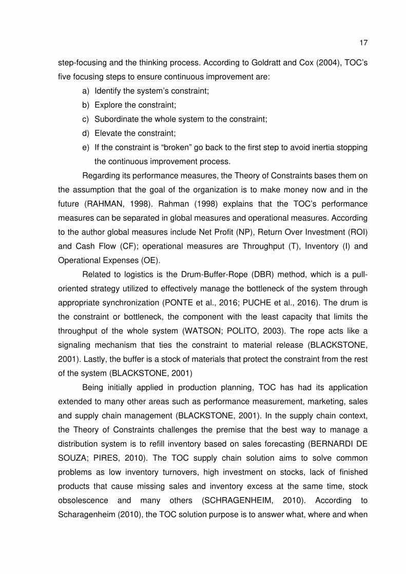
levels to as low as possible (SIMATUPANG; WRIGHT; SRIDHARAN, 2004). Figure 2
demonstrates the basic conflict caused by local and global optimum in the supply
chain.
19
Figure 2 – Conflict between local and global optimum in the supply chain.
Source: Bernardi de Souza and Pires (2010).
According to Schragenheim (2010) the majority of the supply chains are based
on push systems where an entity in a central position (such as manufacturing plant)
make the replenishment decisions and supplies goods to regional warehouses or final
customers. Such configuration depends heavily on forecasting models to predict what,
when and where to stock the necessary goods or productions at specific inventory
locations (shops) (SCHRAGENHEIM, 2010). As stated by Bernardi de Souza e Pires
(2010), if a sale is realized when the transfer of goods to the next link of the chain
occurs, it is created a tendency where each link will try to push inventory to the next
upstream entity of the SC. Smith and Ptak (2010) mention that is known that forecasts
are always wrong and their inaccuracy tends to increase as the more detailed they are
and the longer they look into the future. Scharagenheim (2010) thus presents four
fallacies regarding forecasting, being them: i) the fallacy of disaggregation; ii) the
fallacy of the mean; iii) the fallacy of the variance; and iv) the fallacy of sudden
changes.
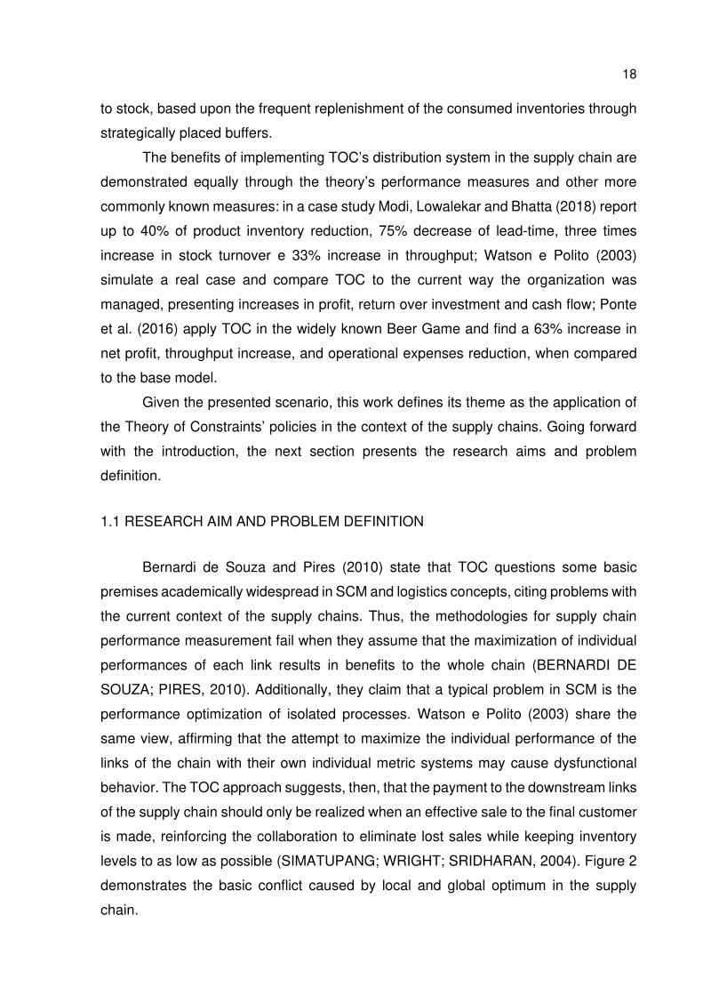
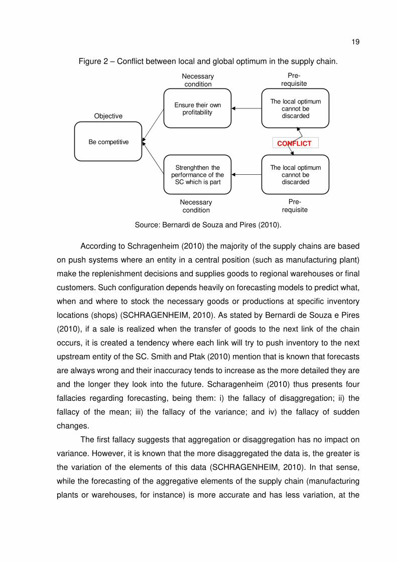
The first fallacy suggests that aggregation or disaggregation has no impact on
variance. However, it is known that the more disaggregated the data is, the greater is
the variation of the elements of this data (SCHRAGENHEIM, 2010). In that sense,
while the forecasting of the aggregative elements of the supply chain (manufacturing
plants or warehouses, for instance) is more accurate and has less variation, at the
CONFLICTBe competitive
Ensure their own profitability
The local optimum cannot be discarded
The local optimum cannot be discarded
Strenghthen the performance of the
SC which is part
Necessarycondition
Necessarycondition
Pre-requisite
Pre-requisite
Objective
20
disaggregated points the effect is the opposite. Figure 3 demonstrates the
mathematical effects of this behavior.
Figure 3 – Mathematical effect of aggregation
Source: Adapted from Scharagenheim (2010).
The second fallacy regards the wrong interpretation of forecasting data.
Schragenheim (2010) states that basic statistical knowledge (mean) is not sufficient
for a full comprehension of the forecasting models and that the lack of a deeper
understanding of those methods may result in huge mistakes. Thus, only a limited
number of people can really understand the concept of variance – the third fallacy –
and standard deviation to determine without a computer their impacts on sales. The
last problem regarding the forecasting methods is related to the sudden changes of
demand: the more sudden the change is the worst the forecast will be
(SCHRAGENHEIM, 2010). The TOC solution for the distribution explores the fact that
forecast accuracy is dependent on the stage (retailers, central warehouses, distribution
centers, manufacturing plants, etc.) of the distribution system (YUAN; CHANG; LI,
2003).
Goldratt (2009) provided the initial concepts about the TOC solution for the
supply chain. The main points proposed by the author are the following: i) the retailers
or shops must keep only the necessary inventory to meet a few days of demand while
21
the rest of the inventory should be kept in a warehouse; ii) the replenishment orders
must be based on actual daily sales in order to avoid shortages of products; iii) the
stock inventory must be kept at and managed by central warehouses, aggregating
demand from shops or retailers, reducing purchase and delivery lead times and the
risk of shortages at the retailers; and iv) the increase inventory turn by purchasing
smaller lots of the same items and selling quickly in order to avoid investing money in
inventory for longer periods. This main concepts and ideas would serve as a base for
the TOC distribution solution. Schragenheim (2010), for instance, provides a few more
insights at the solution, proposing a six-steps method::
a) Stock aggregation at the highest level in the supply chain: the plant/central
warehouse (PWH/CWH);
b) Stock buffer sizes determination for all locations of the chain based on
demand, supply, and replenishment lead time;
c) Increase of the replenishment frequency;
d) Manage the flow of inventories through buffers and buffer penetration;
e) Dynamics Buffer Management (DBM) utilization;
f) Set manufacturing priorities in accordance with the urgency in the plant stock
buffers.
However, even though those steps of the TOC distribution solution aim to solve
many problems related to supply chain management, there are still major gaps to be
addressed by its literature. At the early stages of TOC in the supply chain context,
Perez (1997) claimed that the theory was limited to manufacturing and lacking
extrapolation of its concepts and practices within the SCM theme. Similarly, Blackstone
(2001) affirmed that there is no adequate literature addressing the management of the
supply chain through the Theory of Constraints. Although there is a growing number
of more recent studies discussing the subject, the supply chain and distribution is
where the TOC has been least explored (BERNARDI DE SOUZA; PIRES, 2010).
Likewise, Kaijun and Wang Yuxia (2010) state that while the usage of TOC’s
replenishment system has been growing in companies, the model has not been
described in the literature.
The empirical application of the TOC’s proposed method to validate the
improvements is also a concern. According to Watson and Polito (2003), there is a lack
of formal research to reveal the improvements in the supply chain with the utilization
of TOC’s techniques. Yuan, Chang, and Li (2003) say that there is not a rigorous
22
method to apply the theory practices in real-world applications. Costas et al. (2015)
state that is uncommon to find real supply chain with TOC practices implemented and
therefore more practical examples are needed (FILHO et al., 2016).
Gupta and Snyder (2009) summarize the problems of TOC within SCM claiming
that even though being a methodology that effectively competes with other production
management techniques, TOC’s studies are inconclusive given the lack of: i) realistic
examples; ii) deepness in the considered characteristics; iii) rigor in the applied
methods; and iv) deep statistical analyses. Sharing the author’s view, Tsou (2013)
states that the lack of a rational framework and empirical studies when applied to real
cases refrains the support of TOC in real-world applications. The TOC, however, has
within its literature good examples of: successful applications (KIM; MABIN; DAVIES,
2008; MABIN; BALDERSTONE, 2003), principle dissemination and promotion
(GOLDRATT, 1994, 1997, 2009; GOLDRATT; COX, 2004), and directions for its
implementation (SCHRAGENHEIM, 2010; SCHRAGENHEIM; DETTMER;
PATTERSON, 2009; SMITH; PTAK, 2010). Therefore, it seems that its unacceptance
among the academic community (GUPTA; BOYD, 2008; WATSON; BLACKSTONE;
GARDINER, 2007) is due to the fact that the link between theory and practice is still
absent.
According to Slack, Lewis, and Bates (2004) it is necessary, in operations
management, to reconcile research and practice so that is possible to conceptualize
practice and operationalize theory. Gupta and Boyd (2008) and Naor, Bernardes, and
Coman (2013) affirm that although the TOC is a good theory for the operations
management (OM) context it has not yet been accepted by the OM community. Gupta
and Boyd (2008) claim that is necessary to empirically test the theory behind the TOC
and to analyze the implications and impacts of the theory in the factory and its other
functional areas, such as marketing and accounting. According to Naor, Bernardes,
and Coman (2013), TOC meets the virtues of a good theory: uniqueness, parsimony,
conservation, generalizability, fecundity, internal consistency, empirical riskiness, and
abstraction. Also, problems with the theory reflect the scientific process as expected,
researchers uncover situations where the theory fails and consequently update,
scrutinize, and improve it contributing to the body of knowledge (NAOR; BERNARDES;
COMAN, 2013). In that sense, a claim is made for engagement from the scholars to
debate the TOC, examine empirically its principles, and uncover the domains where
TOC may not hold yet and explain the reasons why it may or may not hold.
23
Another common problem in supply chain management is related to its
measurement systems. Usually, they tend to optimize performance of the individual
processes thus, the goals and the measures to control performance are focused in the
next downstream node of the SC rather than the customer (WATSON; POLITO, 2003).
According to the TOC perspective tough the goal of the whole supply chain is to make
money now and in the future (COSTAS et al., 2015). To achieve the goal, TOC
proposes its operational (T, I, and OE) and global measures (NP, ROI, and CF)
(GOLDRATT; COX, 2004). Within the supply chain context, Goldratt; Schragenheim;
and Ptak (2000) would later include the measures of throughput-dollar-days (TDD) and
inventory-dollar-days (IDD). Those are collaborative performance measures that
guarantee that each node of the SC is doing what is supposed to do to reach the goal
of the system (SIMATUPANG; WRIGHT; SRIDHARAN, 2004). However, the literature
on the TDD and IDD is sparse and inconclusive (GUPTA; ANDERSEN, 2012).
According to Gupta and Andersen (2018) empirical studies and studies that
incorporate TOC implementations and performance measures is still a gap in scientific
research.
Therefore, from the aforementioned studies, three main gaps can be identified:
the lack of a conceptual model or method to apply the TOC’s practices in supply chains
(TSOU, 2013), lack of studies that evaluate consistently the TOC implementation in
supply chains with TOC’s performance measures (GUPTA; ANDERSEN, 2018), and,
consequently, the absence of empirical evidence to support the improvements brought
by the application of theory (GUPTA; BOYD, 2008). More specifically, the TOC supply
chain studies: a) do not measure the contribution of the TOC SC steps, in a holistic or
step-wise manner; b) do not point the causal effects of TOC’s intervention in the supply
chain; c) do not assess systematically the impacts of the TOC in an empirical study;
and d) do not assess the supply chain either in aggregated terms or at each individual
link.
This work uses a real case to address its research problems and fill the gaps
within the TOC supply chain literature. The case is the supply chain of a large-sized
multinational chemical industry that provides goods for the agricultural sector. The
case studies an internal supply chain in the Rio Grande do Sul Brazilian state. The
company is multinational organization with headquarters in Europe, but highly active
in Brazil. The country’s potential is of strategic interest for the organization as,
currently, one third of the company’s global revenue comes from Brazil. The company
24
possesses four production units located in the Brazilian states of Rio Grande do Sul,
Paraná and São Paulo and two central administrative offices. Additionally, the
company has also other 24 mixing units that receive manufactured products from the
production units. The mixing units are spreadly located among eleven Brazilian states.
Many of the raw materials come from Europe from other company’s production units
and international suppliers. Due to the long lead times of the imported raw materials,
the company relies on forecasting to plan production, inventory levels and sales. The
accuracy of forecasting, however, is low – around 60%. This inaccuracy leads to high
inventory values, low inventory turnover, losses to obsolescence, frequent delay in
deliveries and even loss of sales –30 million dollars as estimated by the company. The
application of the TOC concepts in the supply chain aim to solve many of those related
problems (GOLDRATT, 2009; SMITH; PTAK, 2010) therefore, posing itself as an
opportunity to the studied case.
From the clarification of the TOC distribution solution, an overall
contextualization of the theory within the supply chain, and the presented problems
that arise with the theme, the research question that guides this research is defined
as: what are the impacts in supply chain performance when applying TOC practices
for supply chain management?
Having defined the research question, the next sections will present the
research objectives, followed by its academic justification, which aims to enlighten the
relevance of the present work.
1.2 OBJECTIVES
In this section, the general and specific objectives that compose the research are
described.
1.2.1 General Objective
The current work aims to evaluate the impacts of the application of the Theory
of Constraints practices in an MTO supply chain of a chemical industry.

25
1.2.2 Specific Objectives
a) Create and validate a system dynamics model of the current case’s supply
chain with the actual implemented stock and replenishment policies to serve
as the base model;
b) Apply the TOC’s distribution/replenishment solution steps in the base model,
being capable of measuring the impacts of each of the steps in the system
as a whole;
c) Utilize TOC’s performance measures to measure the supply chain redesign
necessary to apply TOC’s supply chain policies;
d) Measure the causal impacts of the TOC’s supply chain polices at each step
application;
1.3 JUSTIFICATION
This section covers the justification of the study considering two different
contexts. The first one, presented in the next sub-section provides its academic
justification, while the second part elaborates its relevance within the enterprise
context. In order to justify the present work in the academic sense, a systematic
literature review was conducted to validate the relevance criteria of the research.
According to Seuring and Gold (2012), the systematic review allows the reviewer to
find relevant information from a growing volume of publications, that might be either
similar or contradictory. The decisions that are made from a series of relevant studies
are more appropriate than those made from a limited set of studies (MORANDI;
CAMARGO, 2015). The relevance, in its turn, can be comprehended as a relation
among two entities, being them: i) a document, part of a document (title, abstract, etc.)
or information; and ii) a problem, information need, request or query – representation
of an information as a system’s language (MIZARRO, 1997). In the current study, the
relevance can be understood as the relation of this research with the problem or gap
to be fulfilled.
The systematic literature review method was applied as suggested by Morandi
e Camargo (2015) and unfolded from the research protocol, presented in Appendix A.
The terms search was made in the EBSCO, ProQuest and Scopus databases and its
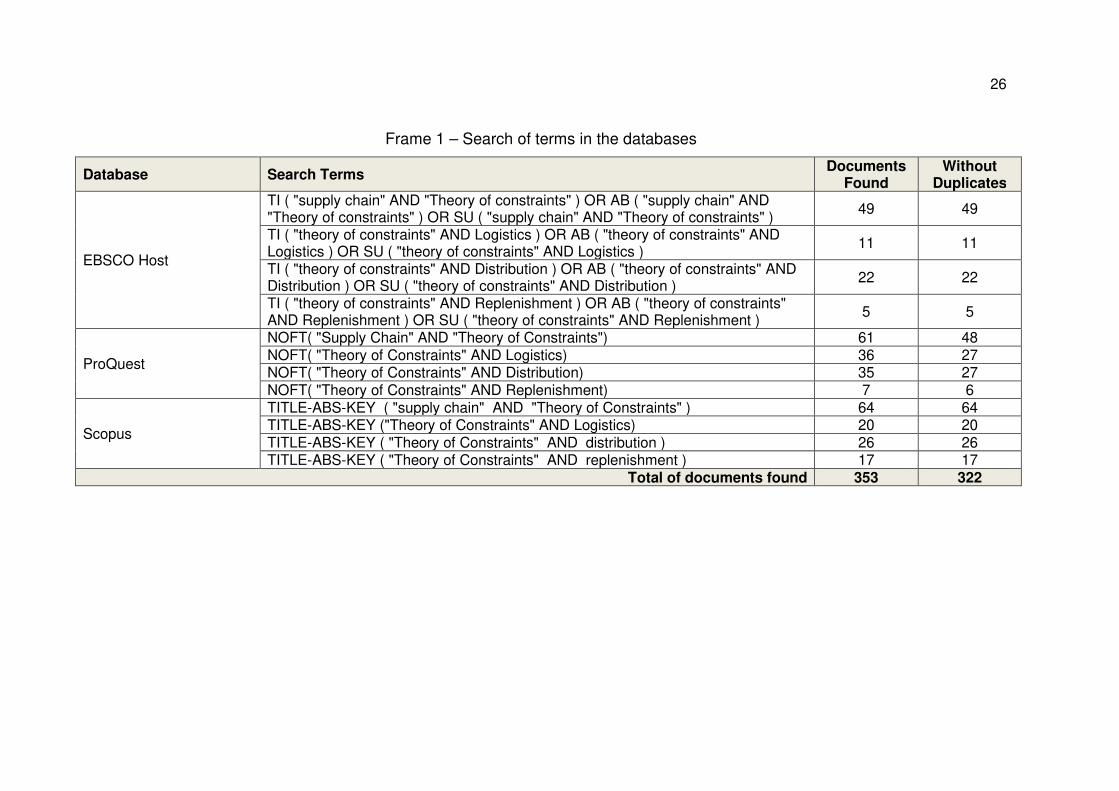
results are presented in Frame 1.
26
Frame 1 – Search of terms in the databases
Database Search Terms Documents
Found Without
Duplicates
EBSCO Host
TI ( "supply chain" AND "Theory of constraints" ) OR AB ( "supply chain" AND "Theory of constraints" ) OR SU ( "supply chain" AND "Theory of constraints" ) 49 49
TI ( "theory of constraints" AND Logistics ) OR AB ( "theory of constraints" AND Logistics ) OR SU ( "theory of constraints" AND Logistics ) 11 11
TI ( "theory of constraints" AND Distribution ) OR AB ( "theory of constraints" AND Distribution ) OR SU ( "theory of constraints" AND Distribution ) 22 22
TI ( "theory of constraints" AND Replenishment ) OR AB ( "theory of constraints" AND Replenishment ) OR SU ( "theory of constraints" AND Replenishment ) 5 5
ProQuest
NOFT( "Supply Chain" AND "Theory of Constraints") 61 48 NOFT( "Theory of Constraints" AND Logistics) 36 27 NOFT( "Theory of Constraints" AND Distribution) 35 27 NOFT( "Theory of Constraints" AND Replenishment) 7 6
Scopus
TITLE-ABS-KEY ( "supply chain" AND "Theory of Constraints" ) 64 64 TITLE-ABS-KEY ("Theory of Constraints" AND Logistics) 20 20 TITLE-ABS-KEY ( "Theory of Constraints" AND distribution ) 26 26 TITLE-ABS-KEY ( "Theory of Constraints" AND replenishment ) 17 17
Total of documents found 353 322
27
In EBSCO host, the terms were searched in the Academic Search Complete,
Business Source Complete and Academic Search Premier databases looking for
matches in titles, abstracts or subjects, being represented by the strings TI, AB and
SU respectively. In ProQuest the terms were searched at any other part of the text with
exception of the text body, this is represented by the search string NOFT. In Scopus,
the searches were conducted by the titles, abstracts or keywords, represented by the
string TITLE-ABS-KEY. Additionally, in all databases the searches were limited to
peer-reviewed academic journals and, in Scopus, an additional limitation to the area
of interest was imposed, limiting the searches to the following areas: i) Business,
Management and Accounting; ii) Engineering; iii) Decision Science; iv) Computer
Science; v) Economics, Econometrics, and Finance; vi) Mathematics; vii) Chemical
Engineering; viii) Energy; ix) Chemistry; and x) Materials Science. In order to get a full
spectrum of the publications, no time restriction was imposed. A total of 353 documents
were of which 31 duplicates were removed, resulting in a total of 322 documents. The
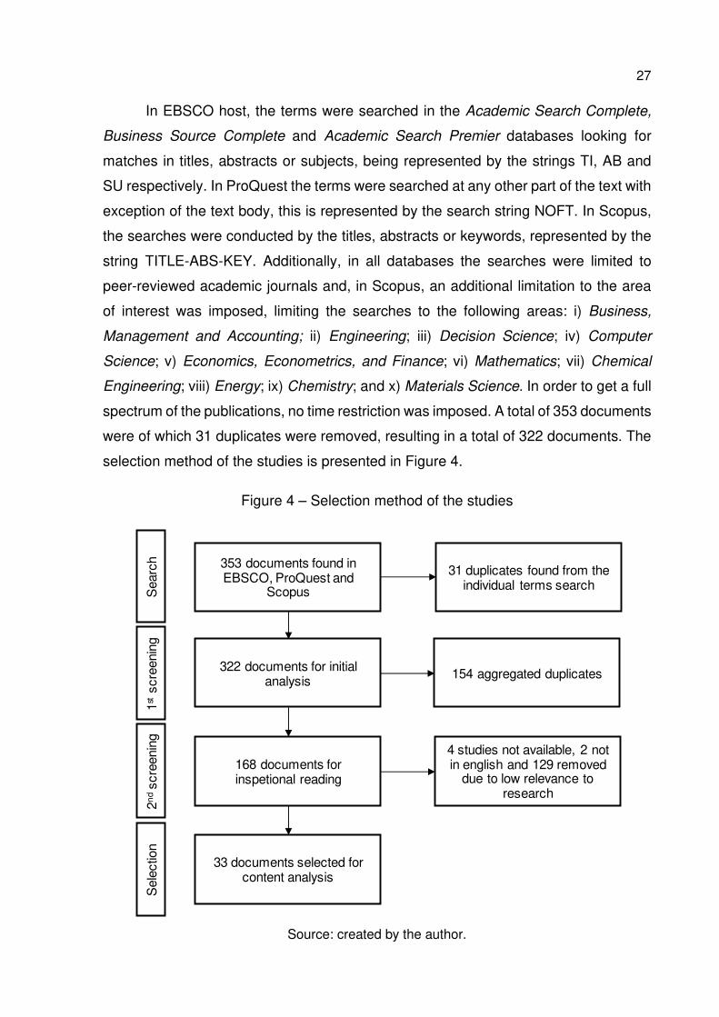
selection method of the studies is presented in Figure 4.
Figure 4 – Selection method of the studies
Source: created by the author.
353 documents found in EBSCO, ProQuest and
Scopus
31 duplicates found from theindividual terms search
322 documents for initial analysis 154 aggregated duplicates
168 documents forinspetional reading
4 studies not available, 2 not in english and 129 removed
due to low relevance to research
33 documents selected for content analysis
Sea
rch
1stsc
reen
ing
2nd
scre
enin
gS
elec
tion
28
After the searches in the databases, the 322 documents found were analyzed
and grouped, and more duplicates were found. The screening resulted in 168 studies
for evaluation of the titles and abstracts. Four studies presented availability limitations,
one study was in Chinese and another one in Spanish, those were removed along with
129 other ones which were excluded due to the low relevance for this study. Those
studies were found to be not relevant for not being related to the focus of this present
research, which included, but are not limited to social themes, governmental/policy
studies, related to healthcare, sustainability focus or other unrelated aspects of the
supply chains.
Those 33 documents were selected for full reading in order to create a literature
overview and identify the current gaps within it. Content analysis is also conducted in
those documents in order to categorize the papers, identify variables and define the
main terms of the theme, providing an overall structure of the literature. Seuring and
Gold (2012) conduct a content analysis in SCM literature and affirm that the structured
and rule-governed procedures of qualitative content analysis compose a powerful tool
to generate valid and reliable results from the literature. Similarly, Jain et al. (2010)
claim that content analysis allows the researcher to define the nature of the content,
find patterns, and estimate relationships among the analyzed literature. The content
analysis is explored in section 2.
Regarding the supply chain, given its complexity, the utilization of simulation
techniques to propose the supply chain redesign is usual (BUIL; PIERA; LASERNA,
2011; ER; MACCARTHY, 2006; FU-REN LIN; YU-HUA PAI, 2000; MARTINS et al.,
2017). Towill (1993a, 1993b) suggests system dynamics as a tool for business
processes redesign; Karagiannaki, Doukidis, and Pramatari (2014) make use of
discrete event simulation (DES) to redesign a supply chain with RFID implementation;
Ponte et al. (2016) utilize Agent-Based Modeling (ABS) to supply chain redesign in
order to reduce the bullwhip effect.
The utilization of TOC and simulation though is more recent: Kaijun, Wang and
Yuxia (2010) simulate the TOC’s buffer management practices for inventory control;
Wu Huang and Jenc (2012) study the replenishment frequency within the Theory of
Constraints context; Costas et al. (2015) apply TOC’s practices in the known Beer
Game case; Gupta and Andersen (2018) utilize DES to apply TOC’s performance
indicators of TDD (throughput-dollar-days) and IDD (inventory-dollar-days) and
analyzed their impacts on the SC. However, this model focus on the TDD and IDD
29
performance measures and actions taken are at the manufacturing level of the supply
chain, not the SC design or structure. Thus, this model does not apply the TOC supply
chain solution, focusing instead in issues such as set-up times, maintenance planning,
and production capacity. The application of the TOC in the supply chain is still limited
though (COSTAS et al., 2015), with a clear gap regarding empirical studies to support
the theory’s practices (TSOU, 2013; WATSON; POLITO, 2003). This study then
provides an empirical study from a real case by the utilization of computational
simulation, defining System Dynamics (SD) as its modeling and simulation tool.
System Dynamics is chosen for this study for being known as a tool that
observes systems from a macro level and is utilized for strategic decision making
(LAW, 2014). According to Sterman (2000), the system dynamics (SD) is concerned
with the behavior of complex systems and requires more than just technical tools for
the creation of mathematical models. Pidd (2003) affirms that the SD is a set of tools
and a simulation approach thought initially for the industrial environment. With one of
its operation methods, the system dynamics makes use of its structural functionalities
to develop a computer simulation model that utilizes quantitative data (PIDD, 2003).
From the system dynamics modeling and the current state of the case will derive the
validation of the model itself and from the validated model new models will be created
to simulate the individual application of the steps of the TOC distribution/replenishment
solution. At the end, once all steps have been applied, it will be able to evaluate the
overall impacts of the whole TOC solution in the supply chain based on traditional
financial measures as well as the TOC’s performance measures. The gradual
application of the steps will allow to assess individually each one of the TOC’s policies,
comparing them and measuring their contribution to the overall impact in the supply
chain as whole.
In order to apply the TOC’s steps it is necessary to change the SC design. This
study aims to define what are the necessary changes in order to fully apply the TOC
model and how long it takes to see the impacts in the supply chain. Also, to better
understand all the impacts caused by this changes the CausalImpact technique is
utilized. According to Brodersen et al. (2015) This technique allows to measure the
causal impacts caused by an intervention in a temporal series, allowing to understand
and compare the application of the TOC steps and the non-application of them.
Therefore, the causal impacts to the supply chain caused by the changes required by
the TOC solution is of interest as well, contributing to fill the gaps of empirical
30
researches (GUPTA; BOYD, 2008; TSOU, 2013) and of evidences of the TOC solution
application (IKEZIRI et al., 2019).
In a general sense, this study also aims to contribute to fulfill the gap of empirical
studies of the TOC literature within the supply chain context as well as contribute with
the application of the distribution/replenishment solution and the analysis of its impacts
in the system as a whole. This study aims also to contribute and to be relevant to the
enterprise context. The current global environment of the supply chains presents great
challenges for the enterprises. Higher levels of productivity, responsiveness, quality
and reliability combined with reduced costs have become the norm to ensure the
survival of companies in an environment containing increases in demand, variability,
and competition (MISHRA et al., 2012). However, many companies still face problems
in their supply chains, such as lost sales, unavailability of many products, stocked
products that are hard to sell, high investment on inventories with low turnover, and
slow response time to changes in demand (MARGARETHA; BUDIASTUTI; SAHRONI,
2017).
To overcome the supply chain challenges many practices, tools, and techniques
were developed in recent times, such as Just-in-Time, MRP and TOC (GUPTA;
SNYDER, 2009). The TOC specifically has covered many problems in the enterprise
context demonstrating proven empirical results such as increased levels of production
while at the same time reducing inventory investment and cycle times (WATSON;
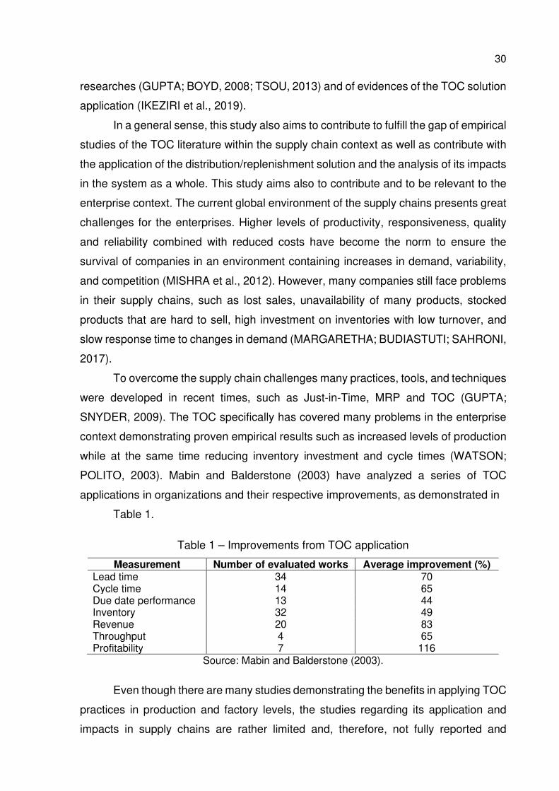
POLITO, 2003). Mabin and Balderstone (2003) have analyzed a series of TOC
applications in organizations and their respective improvements, as demonstrated in
Table 1.
Table 1 – Improvements from TOC application
Measurement Number of evaluated works Average improvement (%) Lead time 34 70 Cycle time 14 65 Due date performance 13 44 Inventory 32 49 Revenue 20 83 Throughput 4 65 Profitability 7 116
Source: Mabin and Balderstone (2003).
Even though there are many studies demonstrating the benefits in applying TOC
practices in production and factory levels, the studies regarding its application and
impacts in supply chains are rather limited and, therefore, not fully reported and
31
comprehended (COSTAS et al., 2015; GUPTA; SNYDER, 2009; IKEZIRI et al., 2019).
Therefore, the relevance of this study within the enterprise context is to validate the
aforementioned improvements of the application of TOC in the supply chain
performance, providing guidance for its implementation and clarifying the expected
results derived from it, based on a real case example. It also extends the TOC supply
chain solution beyond the its initial context – retail and distribution (IKEZIRI et al., 2019)
– to another strategic sector. The case’s business market is at an strategic position in
Brazil, representing 4,36% of the country’s GDP in 2018 (WORLD BANK GROUP,
c2019). This should also contribute to the development and adoption of the theory in
real-world applications, further enhancing the supply chain management performance
of enterprises.
TOC research within the SC perspective have been very specific, focusing on
parts of the replenishment solution such as manufacturing level operations (GUPTA;
ANDERSEN, 2018; TELLES et al., 2019), inventory impacts and improvements
(CHANG; CHANG; HUANG, 2014; CHANG; CHANG; SUN, 2015), buffer management
(TSOU, 2013), and replenishment frequency (WU et al., 2012; WU; LEE; TSAI, 2014).
This research advances the studies of TOC in SCM, by providing a holistic view of its
impacts in the supply chain and its links, analyzing not only its inventory levels, but
also how well positioned are those inventories – using the IDD – and the SC throughput
performance – the TDD. Those measurements are applied at each incremental step of
the solution, being able to: a) assess them individually and synergistically; b) assess
their causal effects probabilities and results at the overall system as well as at its
components; and c) the time it takes from the application of the solution to the observed
effects in the system.
Additionally, this work contributes to the company’s case informing what impacts
and results can be achieved through the TOC method, what is necessary to change in
terms of supply chain design to apply the proposed policies and how long it would take
to perceive the benefits of implementation. It can also contribute to other supply chain
managers, providing a solid and empirical TOC-SCRS study, covering its
implementation, the challenges, the difficulties and especially the expected
improvements. Within the supply chain redesign, it aims to assert TOC’s SC policies
as a sound alternative to be considered in SC redesigns that aim for increased
performance, just other know practices such as lean and JIT.
32
Having presented the academic justification of the research, the next section
covers this study delimitations.
1.4 DELIMITATIONS
Once defined the aim to create a system dynamics model based on the studied
case the delimitation to guide the work should be clarified as well. First, is not the intent
of the work to create a generic model for future studies, in that sense, the proposed
model will relate only to the defined case. Similarly, given the case complexity and its
operations scale, this study will focus on the internal supply chain of the organization
considering all the units located in Rio Grande do Sul state, but not including suppliers
or any other external stakeholders. In that sense, it is also worth mentioning that the
system comprises of an internal supply chain, meaning that all chain links are from the
same organization, which might differ from the general supply chain. However, those
supply chain links are all locally managed with independent and local KPI’s as well,
meaning that the SC behavior is comparable to a common supply chain structure of
independent organizations.
Regarding the Theory of Constraints policies, this research focuses on the
supply chain distribution/replenishment solution steps as proposed by Schragenheim
(2010). It does not include in the system, the manufacturing steps proposed in the
solution, as it is not part of the model. It is not its intent to analyze or apply any other
of the theory’s techniques that are not strictly included in the distribution solution, such
as the thinking process, the critical chain project management, the focusing steps etc.
Having defined the current delimitations, the next section will cover the work structure.
1.5 WORK STRUCTURE
This work is divided into three chapters: Introduction, Theoretical Background,
and Methodological Procedures. In the Introduction, already presented, the initial
discussion regarding the theme is conducted, the research aim and problem definition
are clarified, the specific and general objectives are defined, and the study’s
delimitation is described. In the next section, the Theoretical Background is explored,
where the main terms and concepts are defined, the relevant literature about the theme
is studied through bibliometric and content analyses. Lastly, the section that covers the

33
methodological procedures is presented derived from the goals, objectives, and
delimitations of the research.
34
2 THEORETICAL BACKGROUND
This section presents the main theoretical concepts that ground this study. First,
an overall perspective of the Theory of Constraints is elaborated. Later, focus is given
into the study’s main theme TOC within the supply chain. In order to explore the
subject, both bibliometric analysis and content analysis are conducted. In the
bibliometric analysis, it is possible to observe the evolution of the publications
throughout time, the main journals and terms for those publications, and co-authorship
and cluster analysis. In the content analysis, the selected studies derived from the
systematic literature review are deeply analyzed, defining the main theoretical
concepts, the types and categories of these studies and proving a comprehensive
framework for TOC’s application in the Supply Chain.
2.1 THEORY OF CONSTRAINTS
The Theory of Constraints is a management philosophy which asserts that
constraints determine the performance of a system and that those constraints are
opportunities for continuous improvement of the system (BLACKSTONE, 2001;
PONTE et al., 2016; RAHMAN, 1998). TOC was originated from the Optimized
Production Timetables (OPT) – a software for production schedule – in the late ’70s
(GUPTA, 2003). Since then, the theory has evolved being applied to many aspects of
management in both strategic and operational levels (BASHIRI; TABRIZI, 2010) and
in a wide range of fields as production operations, finance, project management,
supply chain, marketing, among others (BLACKSTONE, 2001).
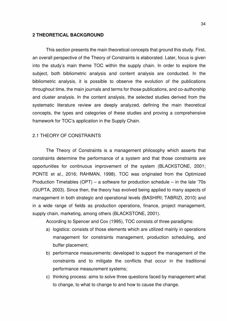
According to Spencer and Cox (1995), TOC consists of three paradigms:
a) logistics: consists of those elements which are utilized mainly in operations
management for constraints management, production scheduling, and
buffer placement;
b) performance measurements: developed to support the management of the
constraints and to mitigate the conflicts that occur in the traditional
performance measurement systems;
c) thinking process: aims to solve three questions faced by management what
to change, to what to change to and how to cause the change.
35
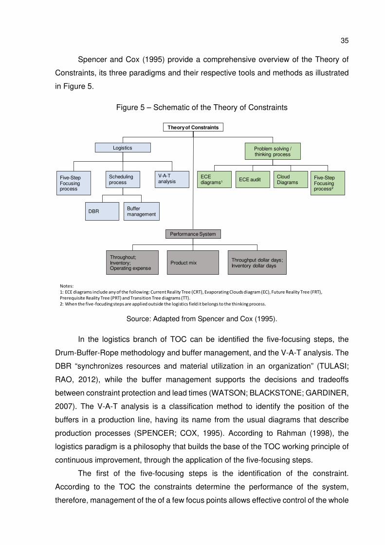
Spencer and Cox (1995) provide a comprehensive overview of the Theory of
Constraints, its three paradigms and their respective tools and methods as illustrated
in Figure 5.
Figure 5 – Schematic of the Theory of Constraints
Source: Adapted from Spencer and Cox (1995).
In the logistics branch of TOC can be identified the five-focusing steps, the
Drum-Buffer-Rope methodology and buffer management, and the V-A-T analysis. The
DBR “synchronizes resources and material utilization in an organization” (TULASI;
RAO, 2012), while the buffer management supports the decisions and tradeoffs
between constraint protection and lead times (WATSON; BLACKSTONE; GARDINER,
2007). The V-A-T analysis is a classification method to identify the position of the
buffers in a production line, having its name from the usual diagrams that describe
production processes (SPENCER; COX, 1995). According to Rahman (1998), the
logistics paradigm is a philosophy that builds the base of the TOC working principle of
continuous improvement, through the application of the five-focusing steps.
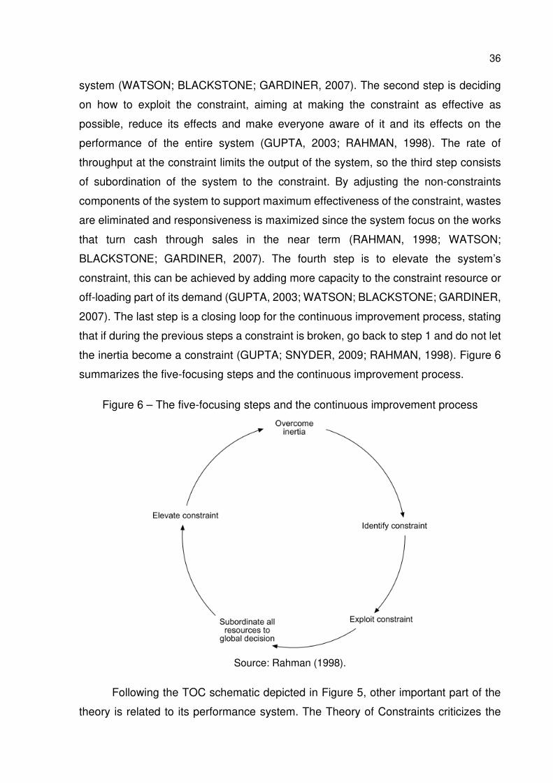
The first of the five-focusing steps is the identification of the constraint.
According to the TOC the constraints determine the performance of the system,
therefore, management of the of a few focus points allows effective control of the whole
Theory of Constraints
Logistics
Performance System
Five-Step Focusing process
Scheduling process
V-A-Tanalysis
DBR Buffer management
Problem solving / thinking process
ECE diagrams¹ ECE audit Cloud
DiagramsFive-Step Focusing process²
Throughout;Inventory;Operating expense
Product mix Throughput dollar days;Inventory dollar days
Notes:
1: ECE diagrams include any of the following: Current Reality Tree (CRT), Evaporating Clouds diagram (EC), Future Reality Tree (FRT),
Prerequisite Reality Tree (PRT) and Transition Tree diagrams (TT).
2: When the five-focuding steps are applied outside the logistics field it belongs to the thinking process.
36
system (WATSON; BLACKSTONE; GARDINER, 2007). The second step is deciding
on how to exploit the constraint, aiming at making the constraint as effective as
possible, reduce its effects and make everyone aware of it and its effects on the
performance of the entire system (GUPTA, 2003; RAHMAN, 1998). The rate of
throughput at the constraint limits the output of the system, so the third step consists
of subordination of the system to the constraint. By adjusting the non-constraints
components of the system to support maximum effectiveness of the constraint, wastes
are eliminated and responsiveness is maximized since the system focus on the works
that turn cash through sales in the near term (RAHMAN, 1998; WATSON;
BLACKSTONE; GARDINER, 2007). The fourth step is to elevate the system’s
constraint, this can be achieved by adding more capacity to the constraint resource or
off-loading part of its demand (GUPTA, 2003; WATSON; BLACKSTONE; GARDINER,
2007). The last step is a closing loop for the continuous improvement process, stating
that if during the previous steps a constraint is broken, go back to step 1 and do not let
the inertia become a constraint (GUPTA; SNYDER, 2009; RAHMAN, 1998). Figure 6
summarizes the five-focusing steps and the continuous improvement process.
Figure 6 – The five-focusing steps and the continuous improvement process
Source: Rahman (1998).
Following the TOC schematic depicted in Figure 5, other important part of the
theory is related to its performance system. The Theory of Constraints criticizes the
37
traditional accounting claiming that this method is obsessed by the need to reduce
operational expense, or as TOC refers to, the cost world thinking (COLWYN JONES;
DUGDALE, 1998). While traditional accounting focuses on cost reduction, the TOC,
on the other hand, focuses on making money now and in the future (WATSON;
BLACKSTONE; GARDINER, 2007). In that sense, the TOC proposes its own
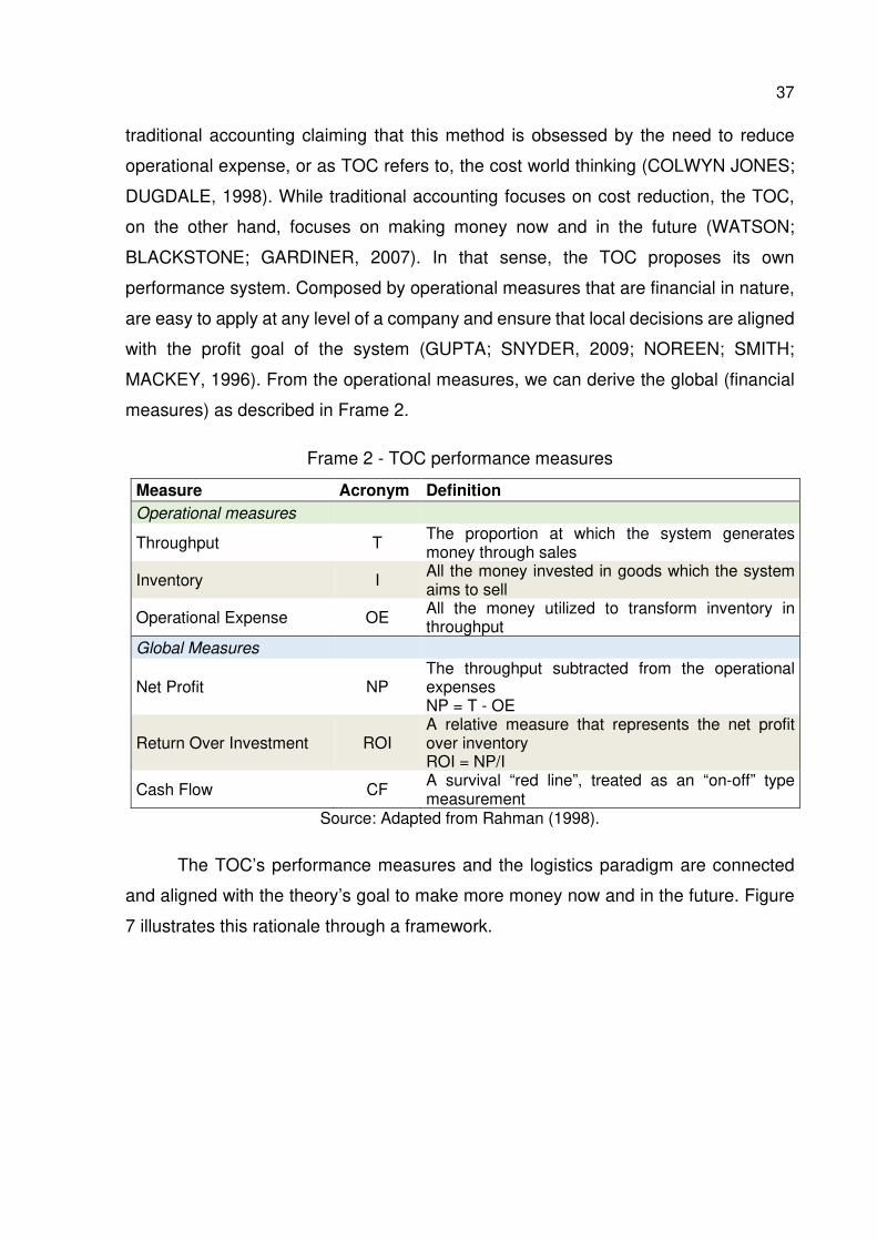
performance system. Composed by operational measures that are financial in nature,
are easy to apply at any level of a company and ensure that local decisions are aligned
with the profit goal of the system (GUPTA; SNYDER, 2009; NOREEN; SMITH;
MACKEY, 1996). From the operational measures, we can derive the global (financial
measures) as described in Frame 2.
Frame 2 - TOC performance measures
Measure Acronym Definition
Operational measures
Throughput T The proportion at which the system generates money through sales
Inventory I All the money invested in goods which the system aims to sell
Operational Expense OE All the money utilized to transform inventory in throughput
Global Measures
Net Profit NP The throughput subtracted from the operational expenses NP = T - OE
Return Over Investment ROI A relative measure that represents the net profit over inventory ROI = NP/I
Cash Flow CF A survival “red line”, treated as an “on-off” type measurement
Source: Adapted from Rahman (1998).
The TOC’s performance measures and the logistics paradigm are connected
and aligned with the theory’s goal to make more money now and in the future. Figure
7 illustrates this rationale through a framework.
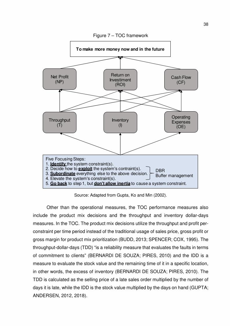
38
Figure 7 – TOC framework
Source: Adapted from Gupta, Ko and Min (2002).
Other than the operational measures, the TOC performance measures also
include the product mix decisions and the throughput and inventory dollar-days
measures. In the TOC. The product mix decisions utilize the throughput and profit per-
constraint per time period instead of the traditional usage of sales price, gross profit or
gross margin for product mix prioritization (BUDD, 2013; SPENCER; COX, 1995). The
throughput-dollar-days (TDD) “is a reliability measure that evaluates the faults in terms
of commitment to clients” (BERNARDI DE SOUZA; PIRES, 2010) and the IDD is a
measure to evaluate the stock value and the remaining time of it in a specific location,
in other words, the excess of inventory (BERNARDI DE SOUZA; PIRES, 2010). The
TDD is calculated as the selling price of a late sales order multiplied by the number of
days it is late, while the IDD is the stock value multiplied by the days on hand (GUPTA;
ANDERSEN, 2012, 2018).
Five Focusing Steps:1. Identify the system constraint(s).2. Decide how to exploit the system's contraint(s).3. Subordinate everything else to the above decision.4. Elevate the system's constraint(s).5. Go back to step 1, but don't allow inertia to cause a system constraint.
DBRBuffer management
Throughput(T)
Inventory (I)
Operating Expenses
(OE)
Cash Flow(CF)
Return on Investiment
(ROI)
Net Profit (NP)
To make more money now and in the future
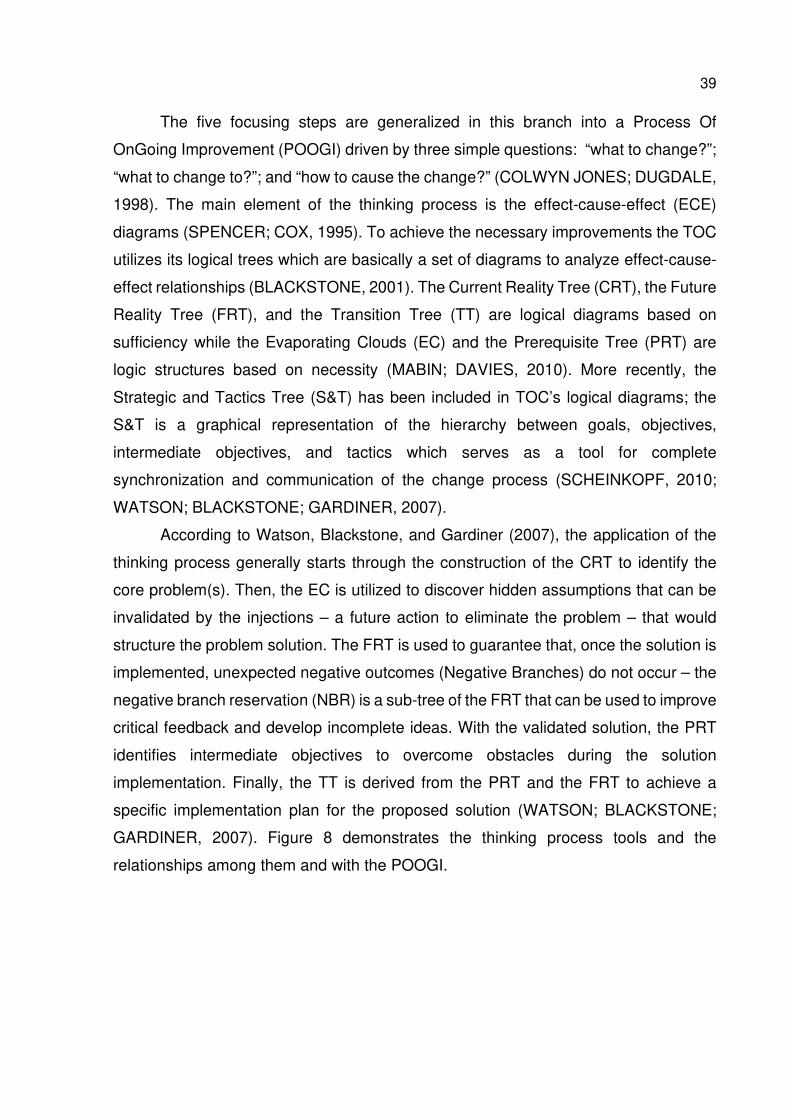
39
The five focusing steps are generalized in this branch into a Process Of
OnGoing Improvement (POOGI) driven by three simple questions: “what to change?”;
“what to change to?”; and “how to cause the change?” (COLWYN JONES; DUGDALE,
1998). The main element of the thinking process is the effect-cause-effect (ECE)
diagrams (SPENCER; COX, 1995). To achieve the necessary improvements the TOC
utilizes its logical trees which are basically a set of diagrams to analyze effect-cause-
effect relationships (BLACKSTONE, 2001). The Current Reality Tree (CRT), the Future
Reality Tree (FRT), and the Transition Tree (TT) are logical diagrams based on
sufficiency while the Evaporating Clouds (EC) and the Prerequisite Tree (PRT) are
logic structures based on necessity (MABIN; DAVIES, 2010). More recently, the
Strategic and Tactics Tree (S&T) has been included in TOC’s logical diagrams; the
S&T is a graphical representation of the hierarchy between goals, objectives,
intermediate objectives, and tactics which serves as a tool for complete
synchronization and communication of the change process (SCHEINKOPF, 2010;
WATSON; BLACKSTONE; GARDINER, 2007).
According to Watson, Blackstone, and Gardiner (2007), the application of the
thinking process generally starts through the construction of the CRT to identify the
core problem(s). Then, the EC is utilized to discover hidden assumptions that can be
invalidated by the injections – a future action to eliminate the problem – that would
structure the problem solution. The FRT is used to guarantee that, once the solution is
implemented, unexpected negative outcomes (Negative Branches) do not occur – the
negative branch reservation (NBR) is a sub-tree of the FRT that can be used to improve
critical feedback and develop incomplete ideas. With the validated solution, the PRT
identifies intermediate objectives to overcome obstacles during the solution
implementation. Finally, the TT is derived from the PRT and the FRT to achieve a
specific implementation plan for the proposed solution (WATSON; BLACKSTONE;
GARDINER, 2007). Figure 8 demonstrates the thinking process tools and the
relationships among them and with the POOGI.
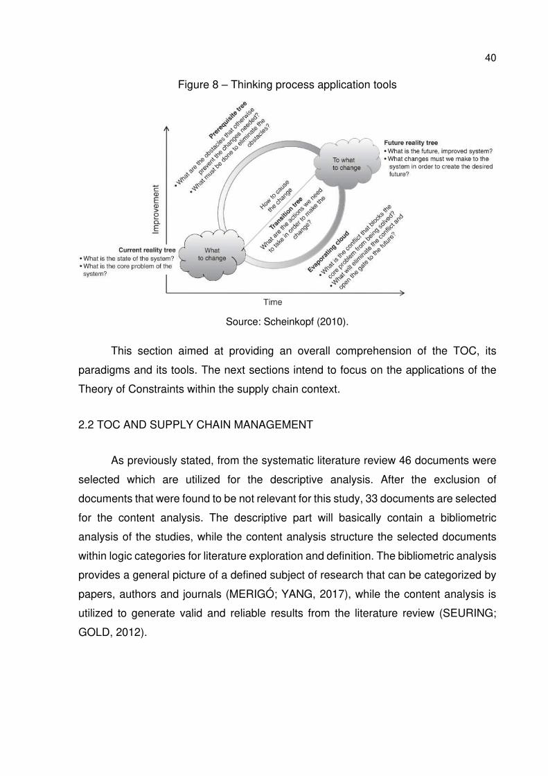
40
Figure 8 – Thinking process application tools
Source: Scheinkopf (2010).
This section aimed at providing an overall comprehension of the TOC, its
paradigms and its tools. The next sections intend to focus on the applications of the
Theory of Constraints within the supply chain context.
2.2 TOC AND SUPPLY CHAIN MANAGEMENT
As previously stated, from the systematic literature review 46 documents were
selected which are utilized for the descriptive analysis. After the exclusion of
documents that were found to be not relevant for this study, 33 documents are selected
for the content analysis. The descriptive part will basically contain a bibliometric
analysis of the studies, while the content analysis structure the selected documents
within logic categories for literature exploration and definition. The bibliometric analysis
provides a general picture of a defined subject of research that can be categorized by
papers, authors and journals (MERIGÓ; YANG, 2017), while the content analysis is
utilized to generate valid and reliable results from the literature review (SEURING;
GOLD, 2012).
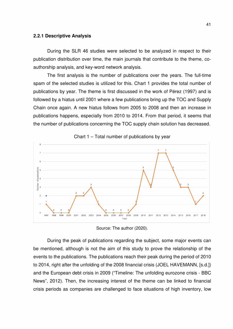
41
2.2.1 Descriptive Analysis
During the SLR 46 studies were selected to be analyzed in respect to their
publication distribution over time, the main journals that contribute to the theme, co-
authorship analysis, and key-word network analysis.
The first analysis is the number of publications over the years. The full-time
spam of the selected studies is utilized for this. Chart 1 provides the total number of
publications by year. The theme is first discussed in the work of Pérez (1997) and is
followed by a hiatus until 2001 where a few publications bring up the TOC and Supply
Chain once again. A new hiatus follows from 2005 to 2008 and then an increase in
publications happens, especially from 2010 to 2014. From that period, it seems that
the number of publications concerning the TOC supply chain solution has decreased.
Chart 1 – Total number of publications by year
Source: The author (2020).
During the peak of publications regarding the subject, some major events can
be mentioned, although is not the aim of this study to prove the relationship of the
events to the publications. The publications reach their peak during the period of 2010
to 2014, right after the unfolding of the 2008 financial crisis (JOEL HAVEMANN, [s.d.])
and the European debt crisis in 2009 (“Timeline: The unfolding eurozone crisis - BBC
News”, 2012). Then, the increasing interest of the theme can be linked to financial
crisis periods as companies are challenged to face situations of high inventory, low
42
turnover, and sudden demand changes (TSOU, 2013) and consequently themes such
as Supply Chain Management become strategically important (COSTAS et al., 2015).
Regarding the periodicals that most contributed to the TOC Supply Chain
Replenishment Solution, Chart 2 presents the number of publications by journals. In
the chart, the journals with one publication only were aggregated in the label “Others”.
It is possible to notice that the International Journal of Production Research is the one
who has more publications, which represents approximately 22% of the publications.
However, the relevant publications of the theme are also widely spread, as 54% of the
journals had published only one paper concerning the subject.
Chart 2 – Number of TOC and supply chain publications by journal
Source: The author (2020).
The main contributor, the International Journal of Production Research is
published since 1961. It is an established, successful and leading journal with
publications related to manufacturing, production, and operations management
research. Currently, the journal has an impact factor of 3,199 according to the Journal
Citation Index.
Going into further detail regarding the most relevant journals it is possible to
double-cross with the distribution of those periodicals throughout the time, which is
presented in Table 2. From the data it is possible to observe that in the period where
most of the publications are concentrated – from 2010 to 2014 – is where most
publications are spread in the “Other” journals categories, meaning that the main
periodicals were not the ones to have more publications. In the mentioned period other
10
3
2
2
2
2
25
0 5 10 15 20 25 30
International Journal of ProductionResearch
Expert Systems with Applications
Journal of Testing and Evaluation
Applied Mechanics and Materials
Computers & Industrial Engineering
Production Planning and Control
Other
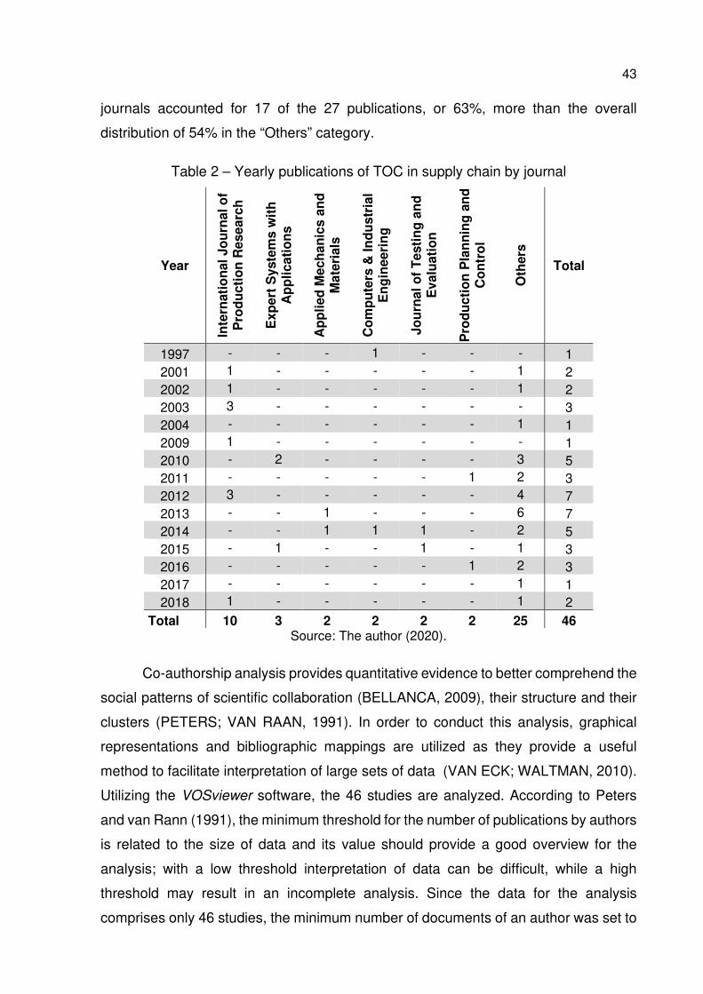
43
journals accounted for 17 of the 27 publications, or 63%, more than the overall
distribution of 54% in the “Others” category.
Table 2 – Yearly publications of TOC in supply chain by journal
Year
Inte
rnati
on
al
Jo
urn
al o
f P
rod
ucti
on
Researc
h
Exp
ert
Syste
ms w
ith
A
pp
licati
on
s
Ap
pli
ed
Mech
an
ics a
nd
M
ate
rials
Co
mp
ute
rs &
In
du
str
ial
En
gin
eeri
ng
Jo
urn
al
of
Testi
ng
an
d
Evalu
ati
on
Pro
du
cti
on
Pla
nn
ing
an
d
Co
ntr
ol
Oth
ers
Total
1997 - - - 1 - - - 1 2001 1 - - - - - 1 2 2002 1 - - - - - 1 2 2003 3 - - - - - - 3 2004 - - - - - - 1 1 2009 1 - - - - - - 1 2010 - 2 - - - - 3 5 2011 - - - - - 1 2 3 2012 3 - - - - - 4 7 2013 - - 1 - - - 6 7 2014 - - 1 1 1 - 2 5 2015 - 1 - - 1 - 1 3 2016 - - - - - 1 2 3 2017 - - - - - - 1 1 2018 1 - - - - - 1 2
Total 10 3 2 2 2 2 25 46 Source: The author (2020).
Co-authorship analysis provides quantitative evidence to better comprehend the
social patterns of scientific collaboration (BELLANCA, 2009), their structure and their
clusters (PETERS; VAN RAAN, 1991). In order to conduct this analysis, graphical
representations and bibliographic mappings are utilized as they provide a useful
method to facilitate interpretation of large sets of data (VAN ECK; WALTMAN, 2010).
Utilizing the VOSviewer software, the 46 studies are analyzed. According to Peters
and van Rann (1991), the minimum threshold for the number of publications by authors
is related to the size of data and its value should provide a good overview for the
analysis; with a low threshold interpretation of data can be difficult, while a high
threshold may result in an incomplete analysis. Since the data for the analysis
comprises only 46 studies, the minimum number of documents of an author was set to
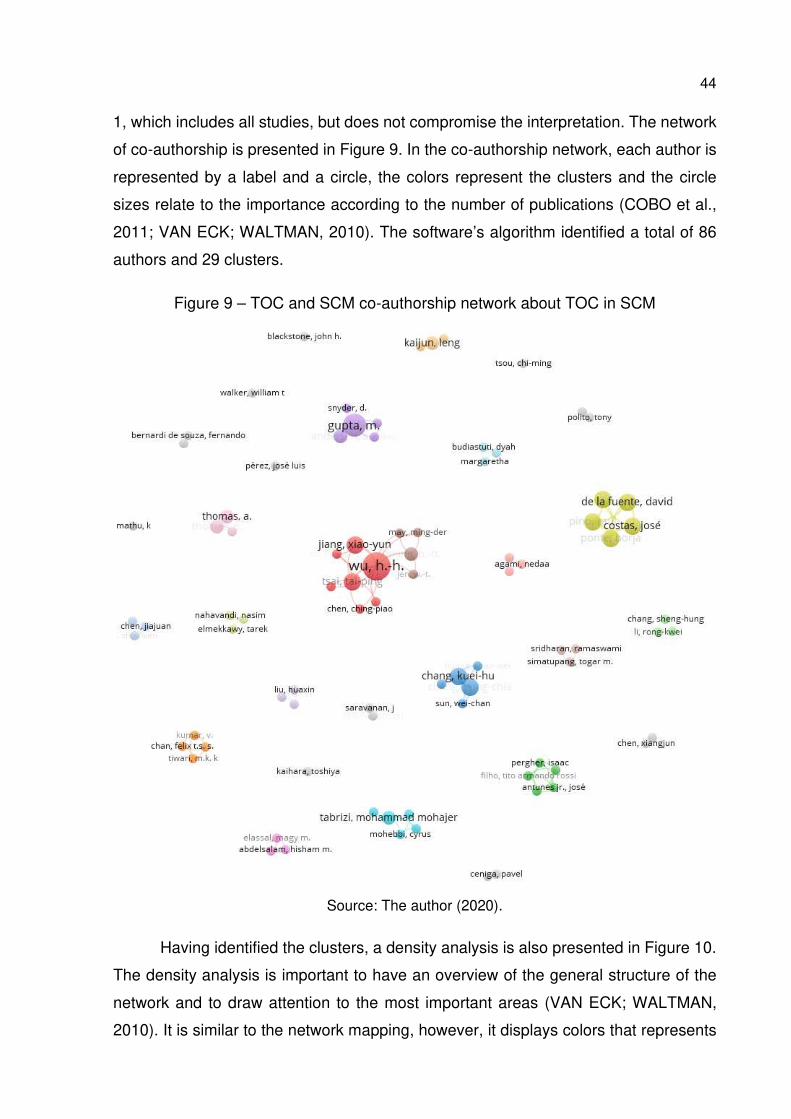
44
1, which includes all studies, but does not compromise the interpretation. The network
of co-authorship is presented in Figure 9. In the co-authorship network, each author is
represented by a label and a circle, the colors represent the clusters and the circle
sizes relate to the importance according to the number of publications (COBO et al.,
2011; VAN ECK; WALTMAN, 2010). The software’s algorithm identified a total of 86
authors and 29 clusters.
Figure 9 – TOC and SCM co-authorship network about TOC in SCM
Source: The author (2020).
Having identified the clusters, a density analysis is also presented in Figure 10.
The density analysis is important to have an overview of the general structure of the
network and to draw attention to the most important areas (VAN ECK; WALTMAN,
2010). It is similar to the network mapping, however, it displays colors that represents
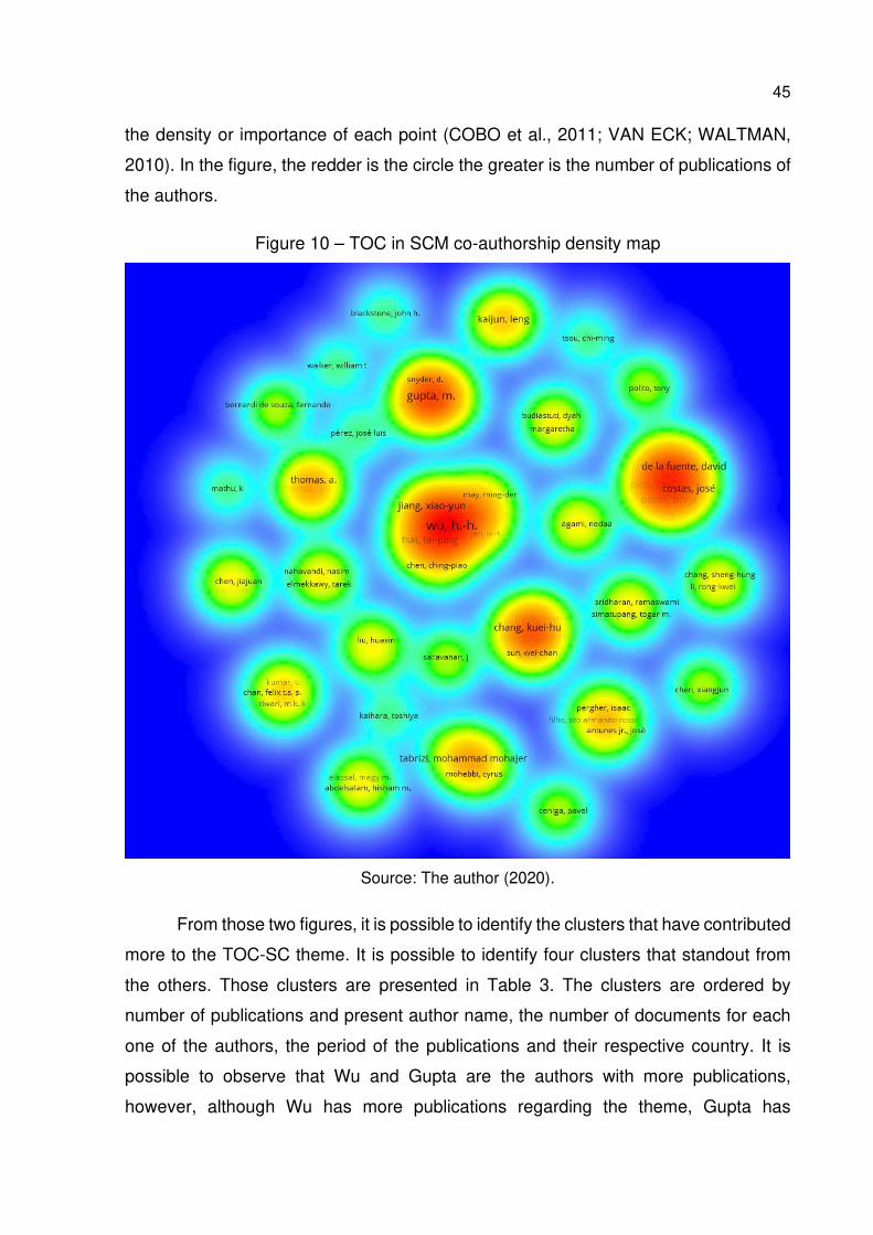
45
the density or importance of each point (COBO et al., 2011; VAN ECK; WALTMAN,
2010). In the figure, the redder is the circle the greater is the number of publications of
the authors.
Figure 10 – TOC in SCM co-authorship density map
Source: The author (2020).
From those two figures, it is possible to identify the clusters that have contributed
more to the TOC-SC theme. It is possible to identify four clusters that standout from
the others. Those clusters are presented in Table 3. The clusters are ordered by
number of publications and present author name, the number of documents for each
one of the authors, the period of the publications and their respective country. It is
possible to observe that Wu and Gupta are the authors with more publications,
however, although Wu has more publications regarding the theme, Gupta has
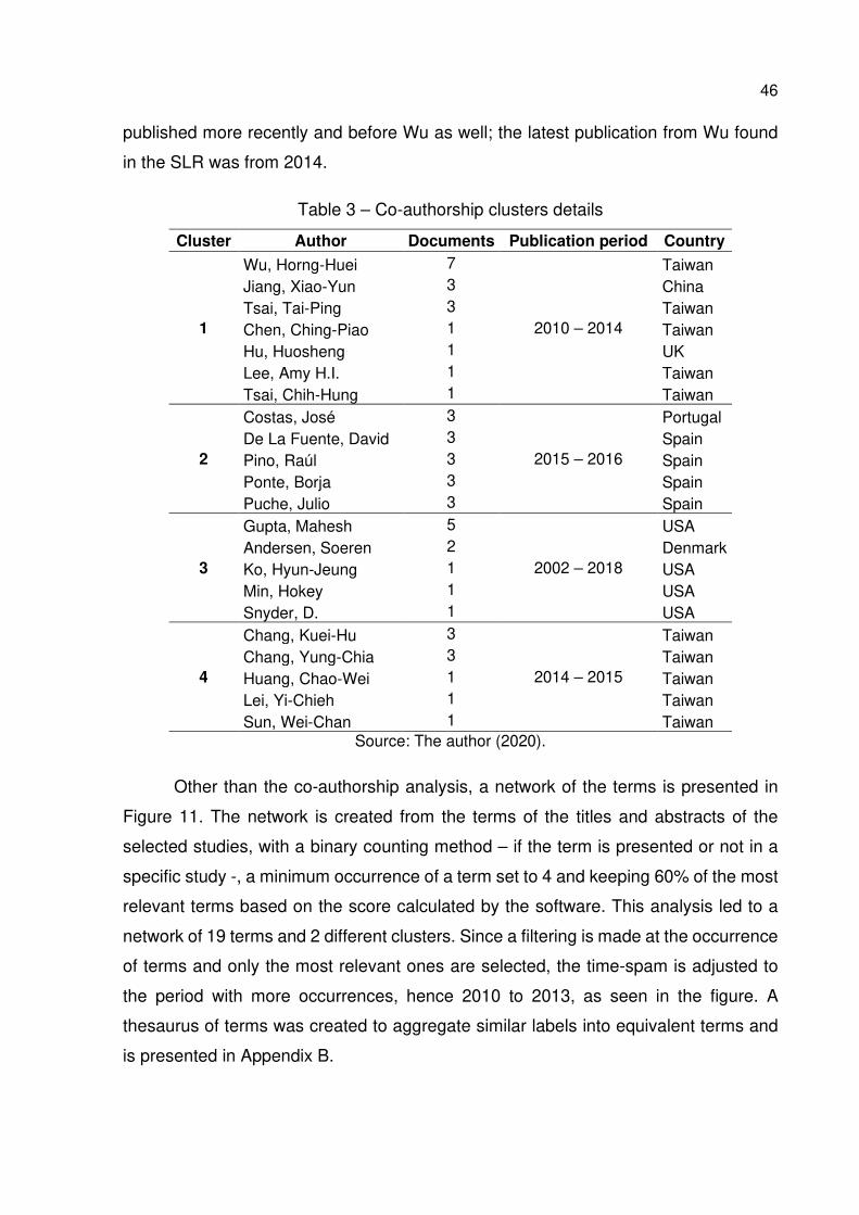
46
published more recently and before Wu as well; the latest publication from Wu found
in the SLR was from 2014.
Table 3 – Co-authorship clusters details
Cluster Author Documents Publication period Country
1
Wu, Horng-Huei 7
2010 – 2014
Taiwan Jiang, Xiao-Yun 3 China Tsai, Tai-Ping 3 Taiwan Chen, Ching-Piao 1 Taiwan Hu, Huosheng 1 UK Lee, Amy H.I. 1 Taiwan Tsai, Chih-Hung 1 Taiwan
2
Costas, José 3
2015 – 2016
Portugal De La Fuente, David 3 Spain Pino, Raúl 3 Spain Ponte, Borja 3 Spain Puche, Julio 3 Spain
3
Gupta, Mahesh 5
2002 – 2018
USA Andersen, Soeren 2 Denmark Ko, Hyun-Jeung 1 USA Min, Hokey 1 USA Snyder, D. 1 USA
4
Chang, Kuei-Hu 3
2014 – 2015
Taiwan Chang, Yung-Chia 3 Taiwan Huang, Chao-Wei 1 Taiwan Lei, Yi-Chieh 1 Taiwan Sun, Wei-Chan 1 Taiwan
Source: The author (2020).
Other than the co-authorship analysis, a network of the terms is presented in
Figure 11. The network is created from the terms of the titles and abstracts of the
selected studies, with a binary counting method – if the term is presented or not in a
specific study -, a minimum occurrence of a term set to 4 and keeping 60% of the most
relevant terms based on the score calculated by the software. This analysis led to a
network of 19 terms and 2 different clusters. Since a filtering is made at the occurrence
of terms and only the most relevant ones are selected, the time-spam is adjusted to
the period with more occurrences, hence 2010 to 2013, as seen in the figure. A
thesaurus of terms was created to aggregate similar labels into equivalent terms and
is presented in Appendix B.
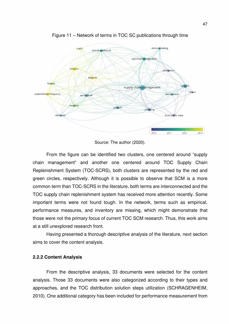
47
Figure 11 – Network of terms in TOC SC publications through time
Source: The author (2020).
From the figure can be identified two clusters, one centered around “supply
chain management” and another one centered around TOC Supply Chain
Replenishment System (TOC-SCRS), both clusters are represented by the red and
green circles, respectively. Although it is possible to observe that SCM is a more
common term than TOC-SCRS in the literature, both terms are interconnected and the
TOC supply chain replenishment system has received more attention recently. Some
important terms were not found tough. In the network, terms such as empirical,
performance measures, and inventory are missing, which might demonstrate that
those were not the primary focus of current TOC SCM research. Thus, this work aims
at a still unexplored research front.
Having presented a thorough descriptive analysis of the literature, next section
aims to cover the content analysis.
2.2.2 Content Analysis
From the descriptive analysis, 33 documents were selected for the content
analysis. Those 33 documents were also categorized according to their types and
approaches, and the TOC distribution solution steps utilization (SCHRAGENHEIM,
2010). One additional category has been included for performance measurement from
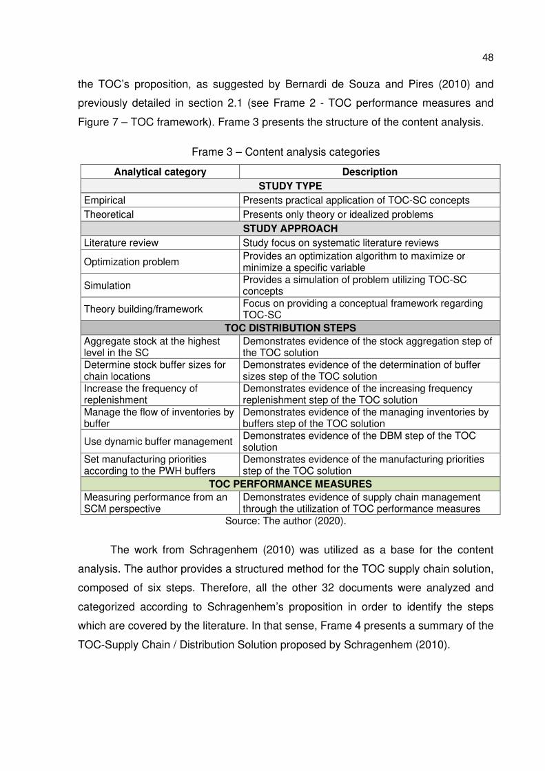
48
the TOC’s proposition, as suggested by Bernardi de Souza and Pires (2010) and
previously detailed in section 2.1 (see Frame 2 - TOC performance measures and
Figure 7 – TOC framework). Frame 3 presents the structure of the content analysis.
Frame 3 – Content analysis categories
Analytical category Description
STUDY TYPE
Empirical Presents practical application of TOC-SC concepts Theoretical Presents only theory or idealized problems
STUDY APPROACH
Literature review Study focus on systematic literature reviews
Optimization problem Provides an optimization algorithm to maximize or minimize a specific variable
Simulation Provides a simulation of problem utilizing TOC-SC concepts
Theory building/framework Focus on providing a conceptual framework regarding TOC-SC
TOC DISTRIBUTION STEPS
Aggregate stock at the highest level in the SC
Demonstrates evidence of the stock aggregation step of the TOC solution
Determine stock buffer sizes for chain locations
Demonstrates evidence of the determination of buffer sizes step of the TOC solution
Increase the frequency of replenishment
Demonstrates evidence of the increasing frequency replenishment step of the TOC solution
Manage the flow of inventories by buffer
Demonstrates evidence of the managing inventories by buffers step of the TOC solution
Use dynamic buffer management Demonstrates evidence of the DBM step of the TOC solution
Set manufacturing priorities according to the PWH buffers
Demonstrates evidence of the manufacturing priorities step of the TOC solution
TOC PERFORMANCE MEASURES
Measuring performance from an SCM perspective
Demonstrates evidence of supply chain management through the utilization of TOC performance measures
Source: The author (2020).
The work from Schragenhem (2010) was utilized as a base for the content
analysis. The author provides a structured method for the TOC supply chain solution,
composed of six steps. Therefore, all the other 32 documents were analyzed and
categorized according to Schragenhem’s proposition in order to identify the steps
which are covered by the literature. In that sense, Frame 4 presents a summary of the
TOC-Supply Chain / Distribution Solution proposed by Schragenhem (2010).
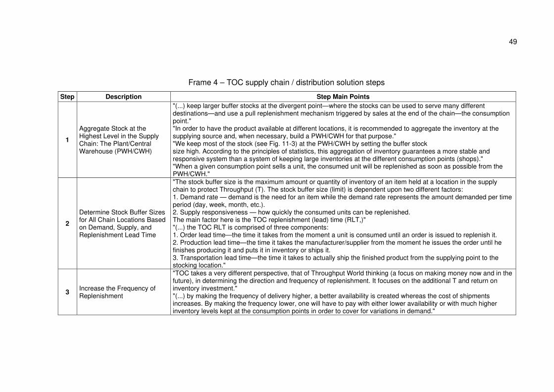
49
Frame 4 – TOC supply chain / distribution solution steps
Step Description Step Main Points
1
Aggregate Stock at the Highest Level in the Supply Chain: The Plant/Central Warehouse (PWH/CWH)
"(...) keep larger buffer stocks at the divergent point—where the stocks can be used to serve many different destinations—and use a pull replenishment mechanism triggered by sales at the end of the chain—the consumption point." "In order to have the product available at different locations, it is recommended to aggregate the inventory at the supplying source and, when necessary, build a PWH/CWH for that purpose." "We keep most of the stock (see Fig. 11-3) at the PWH/CWH by setting the buffer stock size high. According to the principles of statistics, this aggregation of inventory guarantees a more stable and responsive system than a system of keeping large inventories at the different consumption points (shops)." "When a given consumption point sells a unit, the consumed unit will be replenished as soon as possible from the PWH/CWH."
2
Determine Stock Buffer Sizes for All Chain Locations Based on Demand, Supply, and Replenishment Lead Time
"The stock buffer size is the maximum amount or quantity of inventory of an item held at a location in the supply chain to protect Throughput (T). The stock buffer size (limit) is dependent upon two different factors: 1. Demand rate — demand is the need for an item while the demand rate represents the amount demanded per time period (day, week, month, etc.). 2. Supply responsiveness — how quickly the consumed units can be replenished. The main factor here is the TOC replenishment (lead) time (RLT,)" "(...) the TOC RLT is comprised of three components: 1. Order lead time—the time it takes from the moment a unit is consumed until an order is issued to replenish it. 2. Production lead time—the time it takes the manufacturer/supplier from the moment he issues the order until he finishes producing it and puts it in inventory or ships it. 3. Transportation lead time—the time it takes to actually ship the finished product from the supplying point to the stocking location."
3 Increase the Frequency of Replenishment
"TOC takes a very different perspective, that of Throughput World thinking (a focus on making money now and in the future), in determining the direction and frequency of replenishment. It focuses on the additional T and return on inventory investment." "(...) by making the frequency of delivery higher, a better availability is created whereas the cost of shipments increases. By making the frequency lower, one will have to pay with either lower availability or with much higher inventory levels kept at the consumption points in order to cover for variations in demand."
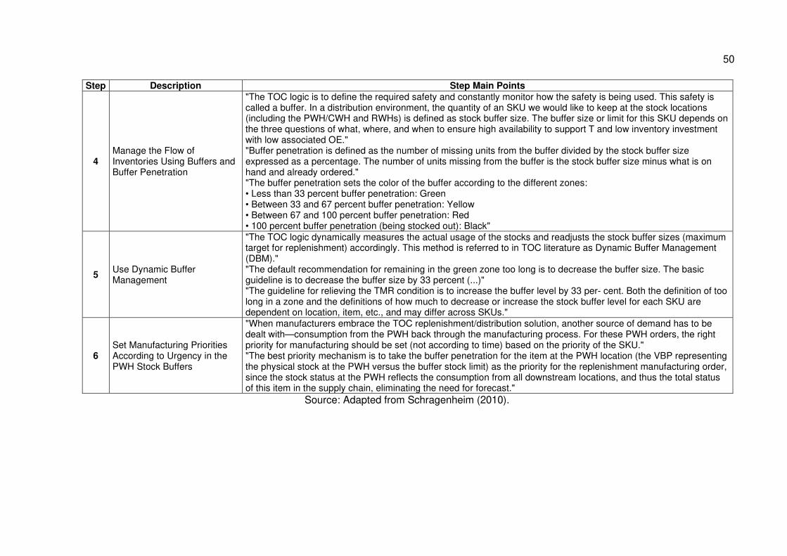
50
Step Description Step Main Points
4 Manage the Flow of Inventories Using Buffers and Buffer Penetration
"The TOC logic is to define the required safety and constantly monitor how the safety is being used. This safety is called a buffer. In a distribution environment, the quantity of an SKU we would like to keep at the stock locations (including the PWH/CWH and RWHs) is defined as stock buffer size. The buffer size or limit for this SKU depends on the three questions of what, where, and when to ensure high availability to support T and low inventory investment with low associated OE." "Buffer penetration is defined as the number of missing units from the buffer divided by the stock buffer size expressed as a percentage. The number of units missing from the buffer is the stock buffer size minus what is on hand and already ordered." "The buffer penetration sets the color of the buffer according to the different zones: • Less than 33 percent buffer penetration: Green • Between 33 and 67 percent buffer penetration: Yellow • Between 67 and 100 percent buffer penetration: Red • 100 percent buffer penetration (being stocked out): Black"
5 Use Dynamic Buffer Management
"The TOC logic dynamically measures the actual usage of the stocks and readjusts the stock buffer sizes (maximum target for replenishment) accordingly. This method is referred to in TOC literature as Dynamic Buffer Management (DBM)." "The default recommendation for remaining in the green zone too long is to decrease the buffer size. The basic guideline is to decrease the buffer size by 33 percent (...)" "The guideline for relieving the TMR condition is to increase the buffer level by 33 per- cent. Both the definition of too long in a zone and the definitions of how much to decrease or increase the stock buffer level for each SKU are dependent on location, item, etc., and may differ across SKUs."
6 Set Manufacturing Priorities According to Urgency in the PWH Stock Buffers
"When manufacturers embrace the TOC replenishment/distribution solution, another source of demand has to be dealt with—consumption from the PWH back through the manufacturing process. For these PWH orders, the right priority for manufacturing should be set (not according to time) based on the priority of the SKU." "The best priority mechanism is to take the buffer penetration for the item at the PWH location (the VBP representing the physical stock at the PWH versus the buffer stock limit) as the priority for the replenishment manufacturing order, since the stock status at the PWH reflects the consumption from all downstream locations, and thus the total status of this item in the supply chain, eliminating the need for forecast."
Source: Adapted from Schragenheim (2010).
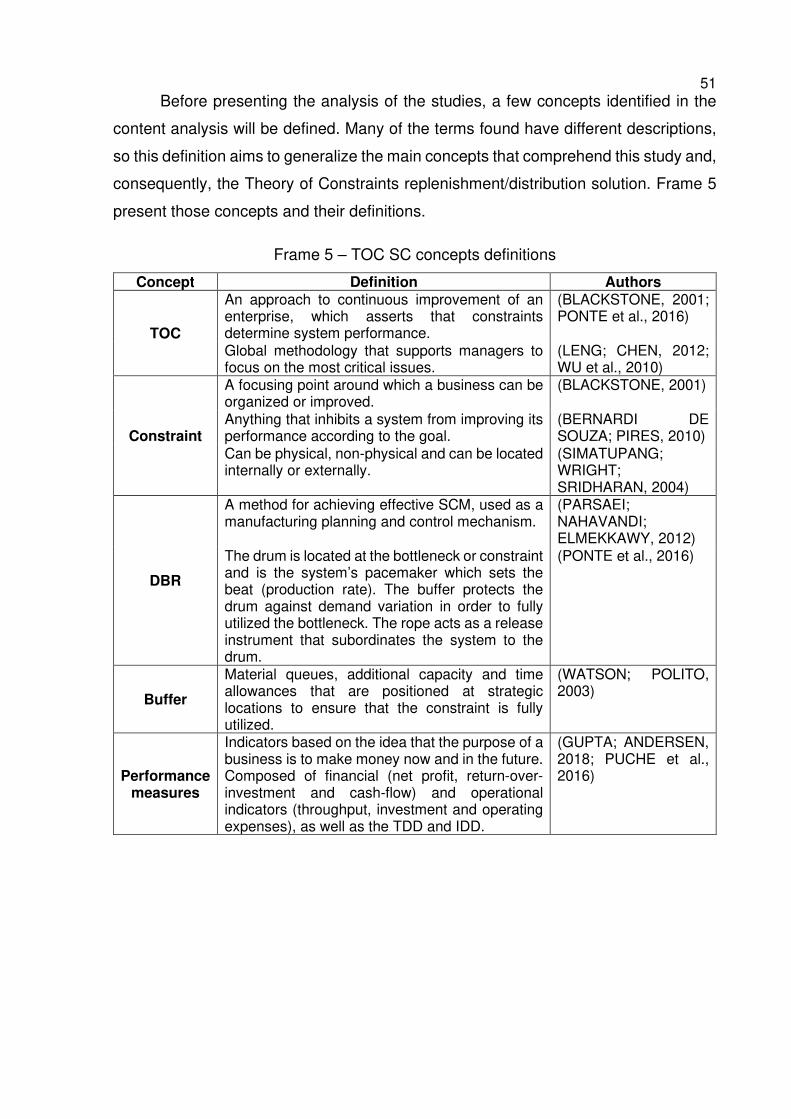
51 Before presenting the analysis of the studies, a few concepts identified in the
content analysis will be defined. Many of the terms found have different descriptions,
so this definition aims to generalize the main concepts that comprehend this study and,
consequently, the Theory of Constraints replenishment/distribution solution. Frame 5
present those concepts and their definitions.
Frame 5 – TOC SC concepts definitions
Concept Definition Authors
TOC
An approach to continuous improvement of an enterprise, which asserts that constraints determine system performance.
(BLACKSTONE, 2001; PONTE et al., 2016)
Global methodology that supports managers to focus on the most critical issues.
(LENG; CHEN, 2012; WU et al., 2010)
Constraint
A focusing point around which a business can be organized or improved.
(BLACKSTONE, 2001)
Anything that inhibits a system from improving its performance according to the goal.
(BERNARDI DE SOUZA; PIRES, 2010)
Can be physical, non-physical and can be located internally or externally.
(SIMATUPANG; WRIGHT; SRIDHARAN, 2004)
DBR
A method for achieving effective SCM, used as a manufacturing planning and control mechanism.
(PARSAEI; NAHAVANDI; ELMEKKAWY, 2012)
The drum is located at the bottleneck or constraint and is the system’s pacemaker which sets the beat (production rate). The buffer protects the drum against demand variation in order to fully utilized the bottleneck. The rope acts as a release instrument that subordinates the system to the drum.
(PONTE et al., 2016)
Buffer
Material queues, additional capacity and time allowances that are positioned at strategic locations to ensure that the constraint is fully utilized.
(WATSON; POLITO, 2003)
Performance measures
Indicators based on the idea that the purpose of a business is to make money now and in the future. Composed of financial (net profit, return-over-investment and cash-flow) and operational indicators (throughput, investment and operating expenses), as well as the TDD and IDD.
(GUPTA; ANDERSEN, 2018; PUCHE et al., 2016)
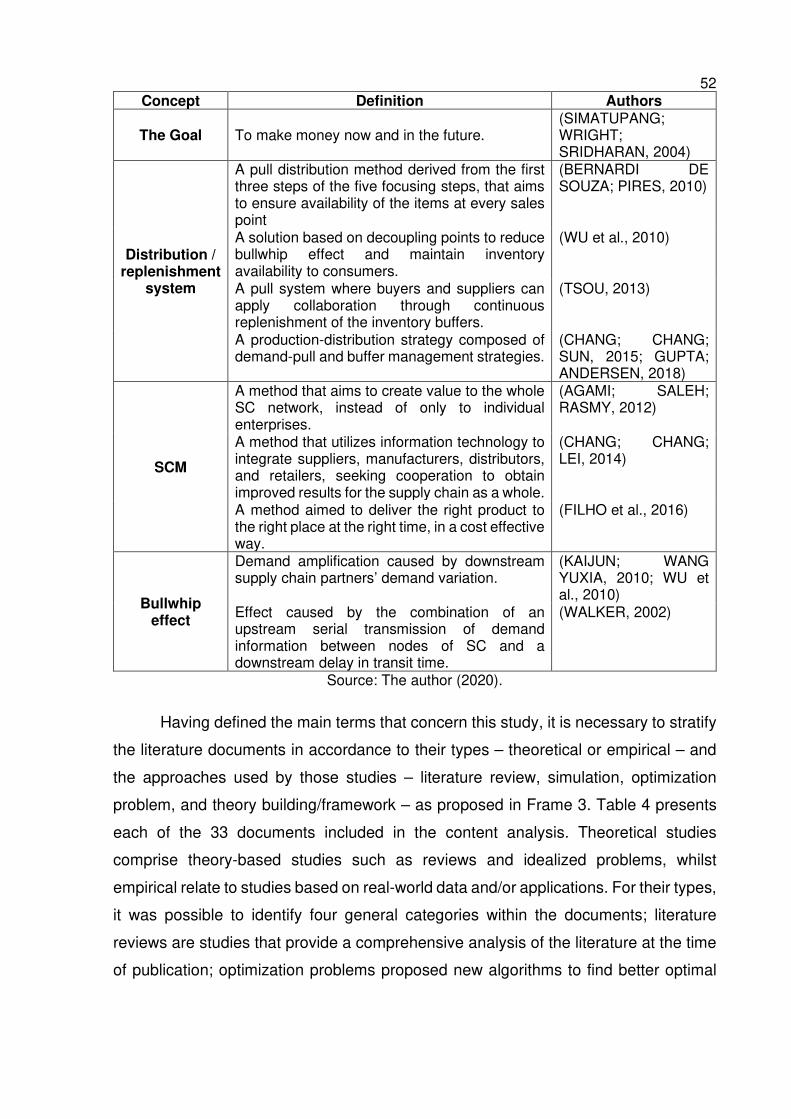
52 Concept Definition Authors
The Goal To make money now and in the future. (SIMATUPANG; WRIGHT; SRIDHARAN, 2004)
Distribution / replenishment
system
A pull distribution method derived from the first three steps of the five focusing steps, that aims to ensure availability of the items at every sales point
(BERNARDI DE SOUZA; PIRES, 2010)
A solution based on decoupling points to reduce bullwhip effect and maintain inventory availability to consumers.
(WU et al., 2010)
A pull system where buyers and suppliers can apply collaboration through continuous replenishment of the inventory buffers.
(TSOU, 2013)
A production-distribution strategy composed of demand-pull and buffer management strategies.
(CHANG; CHANG; SUN, 2015; GUPTA; ANDERSEN, 2018)
SCM
A method that aims to create value to the whole SC network, instead of only to individual enterprises.
(AGAMI; SALEH; RASMY, 2012)
A method that utilizes information technology to integrate suppliers, manufacturers, distributors, and retailers, seeking cooperation to obtain improved results for the supply chain as a whole.
(CHANG; CHANG; LEI, 2014)
A method aimed to deliver the right product to the right place at the right time, in a cost effective way.
(FILHO et al., 2016)
Bullwhip effect
Demand amplification caused by downstream supply chain partners’ demand variation.
(KAIJUN; WANG YUXIA, 2010; WU et al., 2010)
Effect caused by the combination of an upstream serial transmission of demand information between nodes of SC and a downstream delay in transit time.
(WALKER, 2002)
Source: The author (2020).
Having defined the main terms that concern this study, it is necessary to stratify
the literature documents in accordance to their types – theoretical or empirical – and
the approaches used by those studies – literature review, simulation, optimization
problem, and theory building/framework – as proposed in Frame 3. Table 4 presents
each of the 33 documents included in the content analysis. Theoretical studies
comprise theory-based studies such as reviews and idealized problems, whilst
empirical relate to studies based on real-world data and/or applications. For their types,
it was possible to identify four general categories within the documents; literature
reviews are studies that provide a comprehensive analysis of the literature at the time
of publication; optimization problems proposed new algorithms to find better optimal
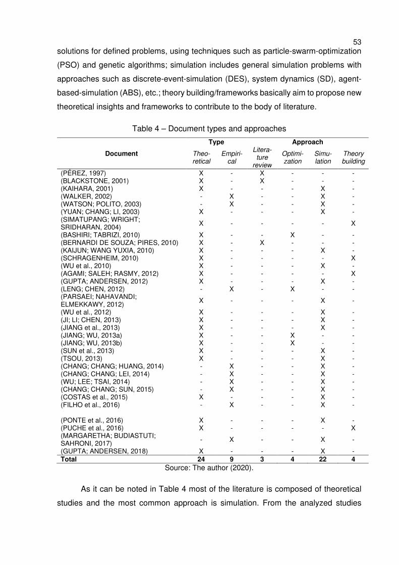
53 solutions for defined problems, using techniques such as particle-swarm-optimization
(PSO) and genetic algorithms; simulation includes general simulation problems with
approaches such as discrete-event-simulation (DES), system dynamics (SD), agent-
based-simulation (ABS), etc.; theory building/frameworks basically aim to propose new
theoretical insights and frameworks to contribute to the body of literature.
Table 4 – Document types and approaches
Document
Type Approach
Theo-retical
Empiri-cal
Litera-ture
review
Optimi-zation
Simu-lation
Theory building
(PÉREZ, 1997) X - X - - - (BLACKSTONE, 2001) X - X - - - (KAIHARA, 2001) X - - - X - (WALKER, 2002) - X - - X - (WATSON; POLITO, 2003) - X - - X - (YUAN; CHANG; LI, 2003) X - - - X - (SIMATUPANG; WRIGHT; SRIDHARAN, 2004) X - - - - X
(BASHIRI; TABRIZI, 2010) X - - X - - (BERNARDI DE SOUZA; PIRES, 2010) X - X - - - (KAIJUN; WANG YUXIA, 2010) X - - - X - (SCHRAGENHEIM, 2010) X - - - - X (WU et al., 2010) X - - - X - (AGAMI; SALEH; RASMY, 2012) X - - - - X (GUPTA; ANDERSEN, 2012) X - - - X - (LENG; CHEN, 2012) - X - X - - (PARSAEI; NAHAVANDI; ELMEKKAWY, 2012) X - - - X -
(WU et al., 2012) X - - - X - (JI; LI; CHEN, 2013) X - - - X - (JIANG et al., 2013) X - - - X - (JIANG; WU, 2013a) X - - X - - (JIANG; WU, 2013b) X - - X - - (SUN et al., 2013) X - - - X - (TSOU, 2013) X - - - X - (CHANG; CHANG; HUANG, 2014) - X - - X - (CHANG; CHANG; LEI, 2014) - X - - X - (WU; LEE; TSAI, 2014) - X - - X - (CHANG; CHANG; SUN, 2015) - X - - X - (COSTAS et al., 2015) X - - - X - (FILHO et al., 2016) - X - - X - (PONTE et al., 2016) X - - - X - (PUCHE et al., 2016) X - - - - X (MARGARETHA; BUDIASTUTI; SAHRONI, 2017) - X - - X -
(GUPTA; ANDERSEN, 2018) X - - - X - Total 24 9 3 4 22 4
Source: The author (2020).
As it can be noted in Table 4 most of the literature is composed of theoretical
studies and the most common approach is simulation. From the analyzed studies
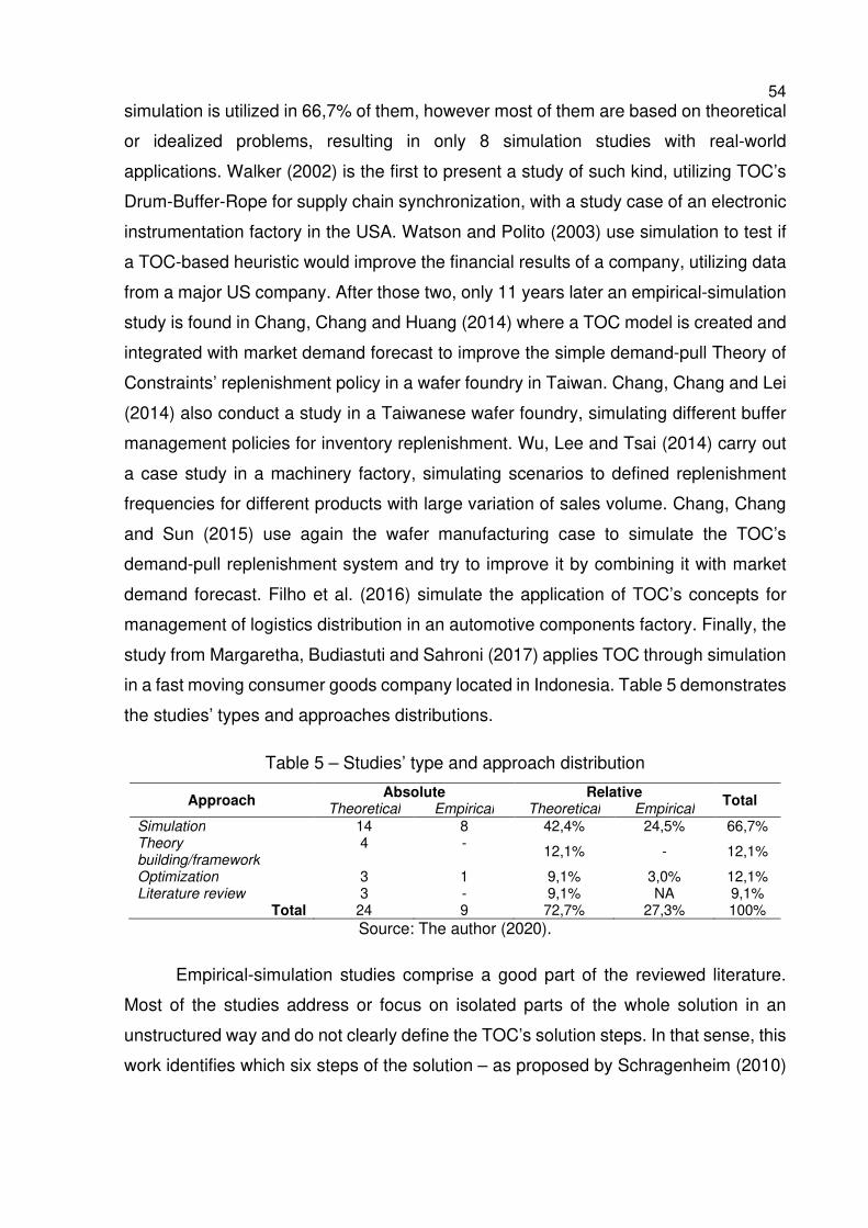
54 simulation is utilized in 66,7% of them, however most of them are based on theoretical
or idealized problems, resulting in only 8 simulation studies with real-world
applications. Walker (2002) is the first to present a study of such kind, utilizing TOC’s
Drum-Buffer-Rope for supply chain synchronization, with a study case of an electronic
instrumentation factory in the USA. Watson and Polito (2003) use simulation to test if
a TOC-based heuristic would improve the financial results of a company, utilizing data
from a major US company. After those two, only 11 years later an empirical-simulation
study is found in Chang, Chang and Huang (2014) where a TOC model is created and
integrated with market demand forecast to improve the simple demand-pull Theory of
Constraints’ replenishment policy in a wafer foundry in Taiwan. Chang, Chang and Lei
(2014) also conduct a study in a Taiwanese wafer foundry, simulating different buffer
management policies for inventory replenishment. Wu, Lee and Tsai (2014) carry out
a case study in a machinery factory, simulating scenarios to defined replenishment
frequencies for different products with large variation of sales volume. Chang, Chang
and Sun (2015) use again the wafer manufacturing case to simulate the TOC’s
demand-pull replenishment system and try to improve it by combining it with market
demand forecast. Filho et al. (2016) simulate the application of TOC’s concepts for
management of logistics distribution in an automotive components factory. Finally, the
study from Margaretha, Budiastuti and Sahroni (2017) applies TOC through simulation
in a fast moving consumer goods company located in Indonesia. Table 5 demonstrates
the studies’ types and approaches distributions.
Table 5 – Studies’ type and approach distribution
Approach Absolute Relative Total
Theoretical Empirical Theoretical Empirical
Simulation 14 8 42,4% 24,5% 66,7% Theory building/framework
4 - 12,1% - 12,1%
Optimization 3 1 9,1% 3,0% 12,1% Literature review 3 - 9,1% NA 9,1%
Total 24 9 72,7% 27,3% 100% Source: The author (2020).
Empirical-simulation studies comprise a good part of the reviewed literature.
Most of the studies address or focus on isolated parts of the whole solution in an
unstructured way and do not clearly define the TOC’s solution steps. In that sense, this
work identifies which six steps of the solution – as proposed by Schragenheim (2010)
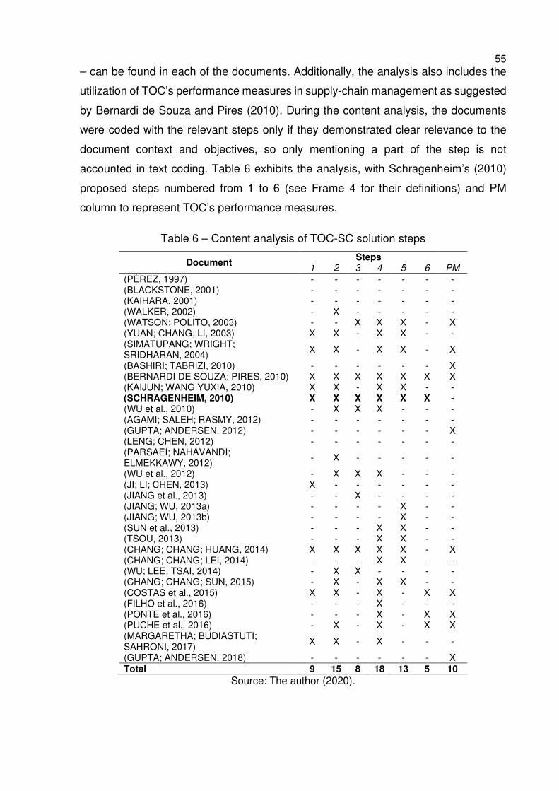
55 – can be found in each of the documents. Additionally, the analysis also includes the
utilization of TOC’s performance measures in supply-chain management as suggested
by Bernardi de Souza and Pires (2010). During the content analysis, the documents
were coded with the relevant steps only if they demonstrated clear relevance to the
document context and objectives, so only mentioning a part of the step is not
accounted in text coding. Table 6 exhibits the analysis, with Schragenheim’s (2010)
proposed steps numbered from 1 to 6 (see Frame 4 for their definitions) and PM
column to represent TOC’s performance measures.
Table 6 – Content analysis of TOC-SC solution steps
Document Steps
1 2 3 4 5 6 PM
(PÉREZ, 1997) - - - - - - - (BLACKSTONE, 2001) - - - - - - - (KAIHARA, 2001) - - - - - - - (WALKER, 2002) - X - - - - - (WATSON; POLITO, 2003) - - X X X - X (YUAN; CHANG; LI, 2003) X X - X X - - (SIMATUPANG; WRIGHT; SRIDHARAN, 2004) X X - X X - X
(BASHIRI; TABRIZI, 2010) - - - - - - X (BERNARDI DE SOUZA; PIRES, 2010) X X X X X X X (KAIJUN; WANG YUXIA, 2010) X X - X X - - (SCHRAGENHEIM, 2010) X X X X X X - (WU et al., 2010) - X X X - - - (AGAMI; SALEH; RASMY, 2012) - - - - - - - (GUPTA; ANDERSEN, 2012) - - - - - - X (LENG; CHEN, 2012) - - - - - - - (PARSAEI; NAHAVANDI; ELMEKKAWY, 2012) - X - - - - -
(WU et al., 2012) - X X X - - - (JI; LI; CHEN, 2013) X - - - - - - (JIANG et al., 2013) - - X - - - - (JIANG; WU, 2013a) - - - - X - - (JIANG; WU, 2013b) - - - - X - - (SUN et al., 2013) - - - X X - - (TSOU, 2013) - - - X X - - (CHANG; CHANG; HUANG, 2014) X X X X X - X (CHANG; CHANG; LEI, 2014) - - - X X - - (WU; LEE; TSAI, 2014) - X X - - - - (CHANG; CHANG; SUN, 2015) - X - X X - - (COSTAS et al., 2015) X X - X - X X (FILHO et al., 2016) - - - X - - - (PONTE et al., 2016) - - - X - X X (PUCHE et al., 2016) - X - X - X X (MARGARETHA; BUDIASTUTI; SAHRONI, 2017) X X - X - - -
(GUPTA; ANDERSEN, 2018) - - - - - - X Total 9 15 8 18 13 5 10
Source: The author (2020).
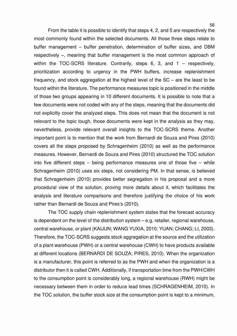
56 From the table it is possible to identify that steps 4, 2, and 5 are respectively the
most commonly found within the selected documents. All those three steps relate to
buffer management – buffer penetration, determination of buffer sizes, and DBM
respectively –, meaning that buffer management is the most common approach of
within the TOC-SCRS literature. Contrarily, steps 6, 3, and 1 – respectively,
prioritization according to urgency in the PWH buffers, increase replenishment
frequency, and stock aggregation at the highest level of the SC – are the least to be
found within the literature. The performance measures topic is positioned in the middle
of those two groups appearing in 10 different documents. It is possible to note that a
few documents were not coded with any of the steps, meaning that the documents did
not explicitly cover the analyzed steps. This does not mean that the document is not
relevant to the topic tough, those documents were kept in the analysis as they may,
nevertheless, provide relevant overall insights to the TOC-SCRS theme. Another
important point is to mention that the work from Bernardi de Souza and Pires (2010)
covers all the steps proposed by Schragenheim (2010) as well as the performance
measures. However, Bernardi de Souza and Pires (2010) structured the TOC solution
into five different steps – being performance measures one of those five – while
Schragenheim (2010) uses six steps, not considering PM. In that sense, is believed
that Schragenheim (2010) provides better segregation in his proposal and a more
procedural view of the solution, proving more details about it, which facilitates the
analysis and literature comparisons and therefore justifying the choice of his work
rather than Bernardi de Souza and Pires’s (2010).
The TOC supply chain replenishment system states that the forecast accuracy
is dependent on the level of the distribution system – e.g. retailer, regional warehouse,
central warehouse, or plant (KAIJUN; WANG YUXIA, 2010; YUAN; CHANG; LI, 2003).
Therefore, the TOC-SCRS suggests stock aggregation at the source and the utilization
of a plant warehouse (PWH) or a central warehouse (CWH) to have products available
at different locations (BERNARDI DE SOUZA; PIRES, 2010). When the organization
is a manufacturer, this point is referred to as the PWH and when the organization is a
distributor then it is called CWH. Additionally, if transportation time from the PWH/CWH
to the consumption point is considerably long, a regional warehouse (RWH) might be
necessary between them in order to reduce lead times (SCHRAGENHEIM, 2010). In
the TOC solution, the buffer stock size at the consumption point is kept to a minimum,
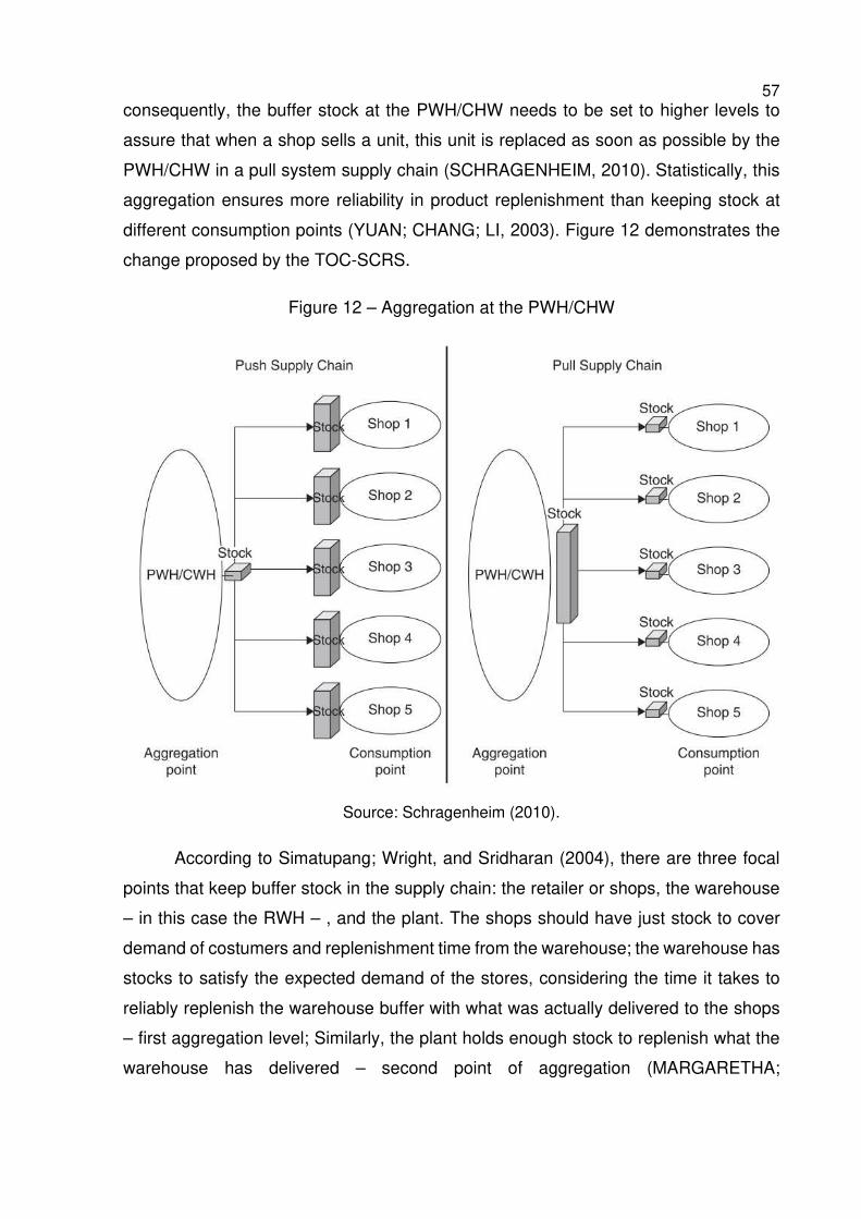
57 consequently, the buffer stock at the PWH/CHW needs to be set to higher levels to
assure that when a shop sells a unit, this unit is replaced as soon as possible by the
PWH/CHW in a pull system supply chain (SCHRAGENHEIM, 2010). Statistically, this
aggregation ensures more reliability in product replenishment than keeping stock at
different consumption points (YUAN; CHANG; LI, 2003). Figure 12 demonstrates the
change proposed by the TOC-SCRS.
Figure 12 – Aggregation at the PWH/CHW
Source: Schragenheim (2010).
According to Simatupang; Wright, and Sridharan (2004), there are three focal
points that keep buffer stock in the supply chain: the retailer or shops, the warehouse
– in this case the RWH – , and the plant. The shops should have just stock to cover
demand of costumers and replenishment time from the warehouse; the warehouse has
stocks to satisfy the expected demand of the stores, considering the time it takes to
reliably replenish the warehouse buffer with what was actually delivered to the shops
– first aggregation level; Similarly, the plant holds enough stock to replenish what the
warehouse has delivered – second point of aggregation (MARGARETHA;
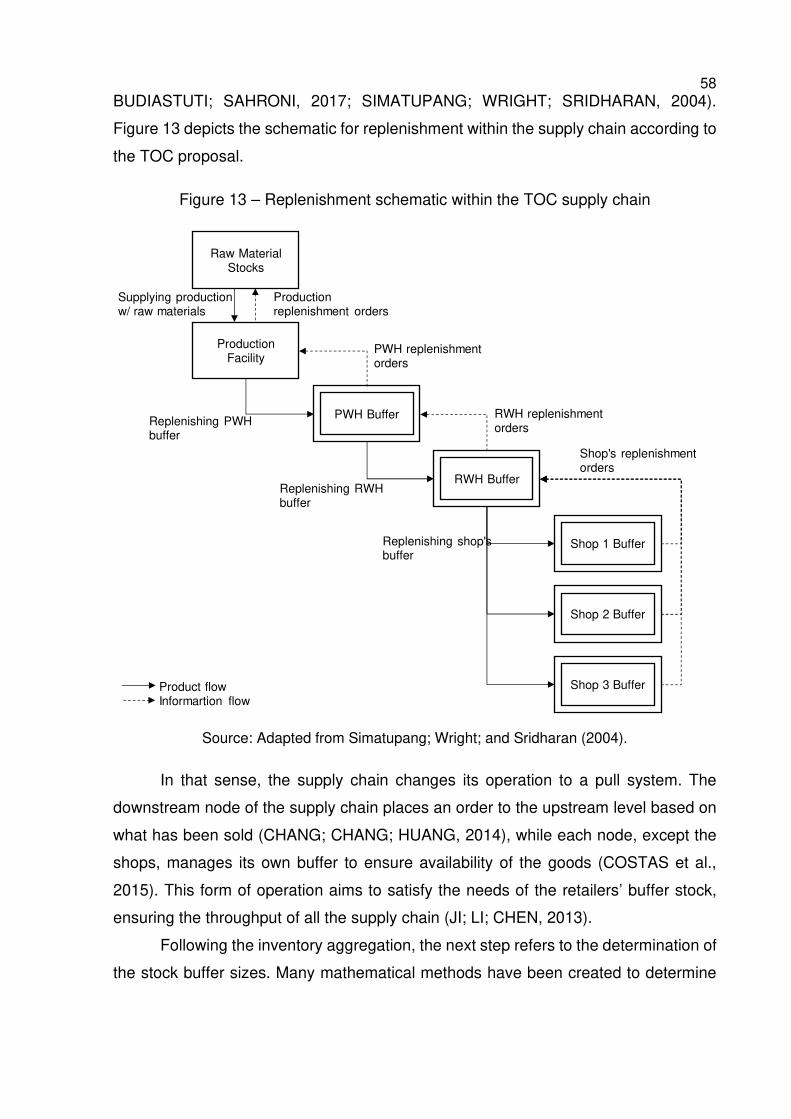
58 BUDIASTUTI; SAHRONI, 2017; SIMATUPANG; WRIGHT; SRIDHARAN, 2004).
Figure 13 depicts the schematic for replenishment within the supply chain according to
the TOC proposal.
Figure 13 – Replenishment schematic within the TOC supply chain
Source: Adapted from Simatupang; Wright; and Sridharan (2004).
In that sense, the supply chain changes its operation to a pull system. The
downstream node of the supply chain places an order to the upstream level based on
what has been sold (CHANG; CHANG; HUANG, 2014), while each node, except the
shops, manages its own buffer to ensure availability of the goods (COSTAS et al.,
2015). This form of operation aims to satisfy the needs of the retailers’ buffer stock,
ensuring the throughput of all the supply chain (JI; LI; CHEN, 2013).
Following the inventory aggregation, the next step refers to the determination of
the stock buffer sizes. Many mathematical methods have been created to determine
Production replenishment orders
Supplying production w/ raw materials
Raw Material Stocks
Production Facility
PWH Buffer
RWH Buffer
Shop 1 Buffer
Shop 2 Buffer
Shop 3 Buffer
Replenishing PWH buffer
PWH replenishment orders
Replenishing RWH buffer
RWH replenishmentorders
Replenishing shop's buffer
Shop's replenishment orders
Product flowInformartion flow
59 the buffer sizes in the supply chain locations (KAIJUN; WANG YUXIA, 2010; YUAN;
CHANG; LI, 2003), however, in TOC setting the exact buffer size is not an relevant
issue as long as the buffer is monitored in a timely manner (YUAN; CHANG; LI, 2003).
Basically, the buffer size is the maximum quantity of stock of an item, kept at each
point of the supply chain to protect the throughput or, in other words, ensure that every
potential customer will have its demand met (BERNARDI DE SOUZA; PIRES, 2010;
CHANG; CHANG; HUANG, 2014; SCHRAGENHEIM, 2010).
According to Schragenheim (2010), the maximum stock buffer size is dependent
on demand rate and supply responsiveness. The demand rate is the demand of an
item per period (day, week, month, etc.). Supply responsiveness refers to how quickly
consumed units can be replenished, represent by the replenishment lead time (RLT).
Parsaei; Nahavandi; and Elmekkawy (2012), Simatupang; Wright; and Sridharan
(2004), and Yuan; Chang; and Li (2003), add a safety factor to be considered to provide
additional protection for unexpected demand and allowing buffer replenishment in time,
without losing throughput. Additionally, Bernardi de Souza and Pires (2010) mention a
few other variables may be considered in the buffer size determination, such as:
average demand within replenishment time, fluctuations of demand, fluctuations of
replenishment time, customer tolerance time, among others.
The replenishment lead time (RLT) has a major role in the buffer size
determination. The TOC RLT has three components: order lead time (OLT), production
lead time (PLT) and transportation lead time (TLT) (BERNARDI DE SOUZA; PIRES,
2010; SCHRAGENHEIM, 2010). The OLT refers to the time it takes to issue an order
of an item from the moment of its consumption; the PLT is the time between the order
issuing until its production has been finished; and the TLT is the time from actually
shipping the item from the supplying point to the stocking location. The TOC solution
aims to reduce the RLT to a minimum in order to generate desired effects such as
reduction of stock required to cover demand during lead time at consumption points,
less fluctuations in supply time, more accurate forecasts due to the reduced time
interval needed, and increase overall responsiveness of the supply chain (BERNARDI
DE SOUZA; PIRES, 2010; SCHRAGENHEIM, 2010). Although important, the RLT has
not been much discussed within the literature. Many studies aim to create
mathematical methods for buffer size determination and only consider RLT as part of
the model, even though, as previously stated, this is not a critical point to the TOC
60 solution. Such studies are those of Chang, Chang, and Sun (2015), Walker (2002), Wu
et al. (2010), Wu, Huang, and Jen (2012), and Wu, Lee, and Tsai (2014).
TOC-SCRS states that items should be replenished based on actual
consumption rather than forecasting. In order to do so, it is necessary to use
replenishment policies based on either daily or the smallest economically feasible
order period (WATSON; POLITO, 2003). The PWH is an important factor to accomplish
this, as it allows the factory to cover replenishment orders directly from its stock without
having to produce this specific item even when that item is available in other client’s
inventory (BERNARDI DE SOUZA; PIRES, 2010).
Increasing the replenishment frequency may be a challenge as suppliers are
accustomed to supply large lot sizes and to pursue high usage of production capacity
(CHANG; CHANG; HUANG, 2014). According to Schragenheim (2010), differently
than the traditional perspective based on economies of scale, the TOC proposal
focuses on the additional throughput (T) and the return over investment (ROI). The
author claims that there is a tradeoff between the additional costs of increasing the
frequency of shipments and the cost of having lower availability. Also, in many cases
the frequent transportation will not cost more than the large-sized shipments as instead
of having large quantities of few products one can have small quantities of many
products. In most cases, the additional revenue obtained will compensate the incurred
extra cost.
The benefits from increasing the replenishment frequency can be seen in the
studies of Jiang et al. (2013) and Wu, Lee, and Tsai (2014). They propose to increase
the replenishment frequency of high demand products and simulate the results. Jiang
et al. (2013) utilizes an optimization algorithm to shorten the replenishment frequency
based on each product demand, while Wu, Lee, and Tsai (2014) simulate an empirical
case applying similar rules. Both report reduction of inventories and economic benefits
while meeting demand requirements and considering capacity constraints,
demonstrating the benefits of increasing the replenishment frequency. Concluded the
discussion on the replenishment frequency, next TOC SC step refers to the inventory
management and buffer penetration.
Buffer size reflects the pattern of the stock consumption level, therefore, buffer
monitoring needs be constant at all time in order to make the decisions about the timing
of production and replenishment (TSOU, 2013). In that sense, monitoring the buffer
61 constantly should ensure that the flow of inventory within the supply chain is moved
accordingly so that each SKU is replenished on time at the consumption points
(PONTE et al., 2016; PUCHE et al., 2016). Thus, the buffer monitoring is a constant
state of progression of the contents of the buffer (WATSON; POLITO, 2003).
Buffer monitoring is realized through the buffer penetration, which is the
percentage relation between the missing units from the buffer and the stock buffer size
(SCHRAGENHEIM, 2010). Usually, the buffers are divided into three distinct zones
containing one third of the stock buffer size and colored differently as green, yellow
and red (CHANG; CHANG; SUN, 2015; CHANG; CHANG; LEI, 2014; SIMATUPANG;
WRIGHT; SRIDHARAN, 2004; YUAN; CHANG; LI, 2003). The colors are set according
to the buffer penetration level: green is for less than 33%, yellow is when it is between
33 and 67%, and red when it is greater than 67% (SCHRAGENHEIM, 2010; YUAN;
CHANG; LI, 2003). This color schematic serves as an indication of replenishment
urgency (BERNARDI DE SOUZA; PIRES, 2010) and its model within the supply chain
is depicted in Figure 14:
a) Green: means that the on-hand inventory is almost up its theoretical
maximum;
b) Yellow: represents the intermediate level, where the normal on-hand
inventory should remain
c) Red: indicates that there is a risk of not meeting the entire demand.
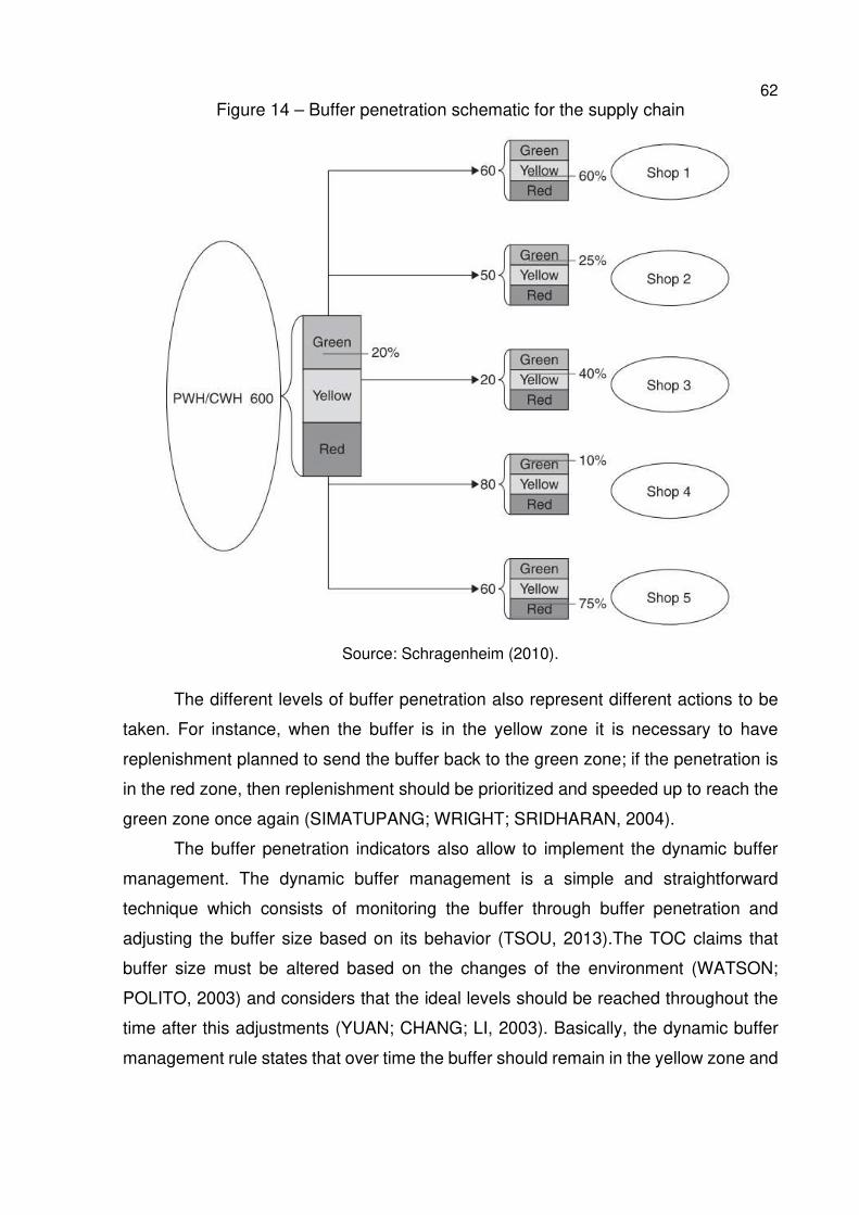
62 Figure 14 – Buffer penetration schematic for the supply chain
Source: Schragenheim (2010).
The different levels of buffer penetration also represent different actions to be
taken. For instance, when the buffer is in the yellow zone it is necessary to have
replenishment planned to send the buffer back to the green zone; if the penetration is
in the red zone, then replenishment should be prioritized and speeded up to reach the
green zone once again (SIMATUPANG; WRIGHT; SRIDHARAN, 2004).
The buffer penetration indicators also allow to implement the dynamic buffer
management. The dynamic buffer management is a simple and straightforward
technique which consists of monitoring the buffer through buffer penetration and
adjusting the buffer size based on its behavior (TSOU, 2013).The TOC claims that
buffer size must be altered based on the changes of the environment (WATSON;
POLITO, 2003) and considers that the ideal levels should be reached throughout the
time after this adjustments (YUAN; CHANG; LI, 2003). Basically, the dynamic buffer
management rule states that over time the buffer should remain in the yellow zone and
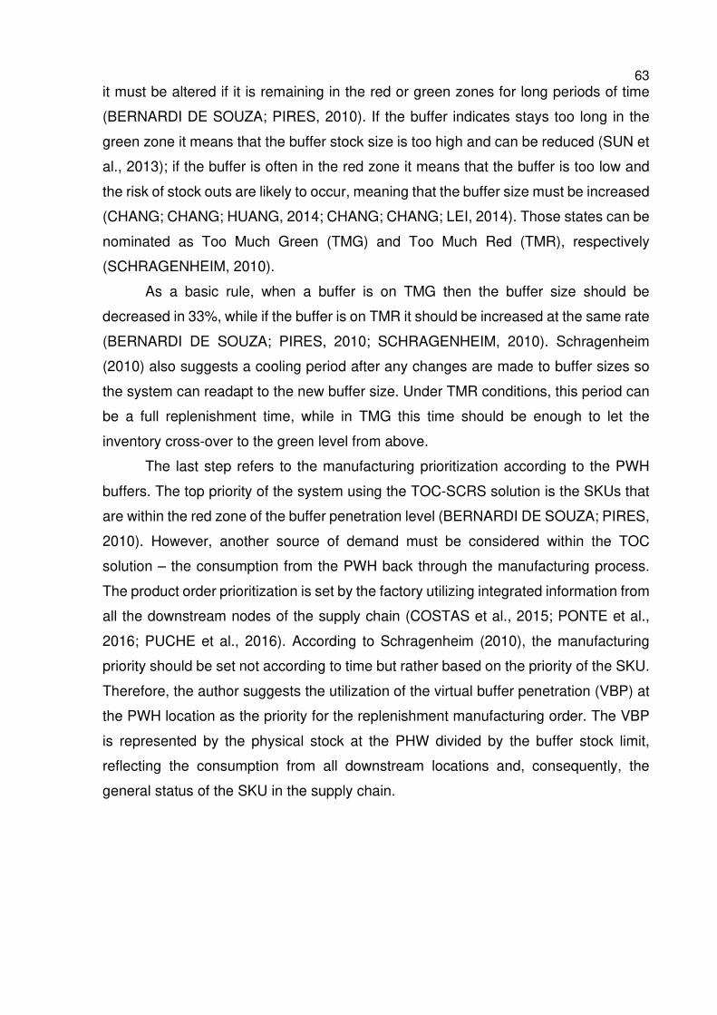
63 it must be altered if it is remaining in the red or green zones for long periods of time
(BERNARDI DE SOUZA; PIRES, 2010). If the buffer indicates stays too long in the
green zone it means that the buffer stock size is too high and can be reduced (SUN et
al., 2013); if the buffer is often in the red zone it means that the buffer is too low and
the risk of stock outs are likely to occur, meaning that the buffer size must be increased
(CHANG; CHANG; HUANG, 2014; CHANG; CHANG; LEI, 2014). Those states can be
nominated as Too Much Green (TMG) and Too Much Red (TMR), respectively
(SCHRAGENHEIM, 2010).
As a basic rule, when a buffer is on TMG then the buffer size should be
decreased in 33%, while if the buffer is on TMR it should be increased at the same rate
(BERNARDI DE SOUZA; PIRES, 2010; SCHRAGENHEIM, 2010). Schragenheim
(2010) also suggests a cooling period after any changes are made to buffer sizes so
the system can readapt to the new buffer size. Under TMR conditions, this period can
be a full replenishment time, while in TMG this time should be enough to let the
inventory cross-over to the green level from above.
The last step refers to the manufacturing prioritization according to the PWH
buffers. The top priority of the system using the TOC-SCRS solution is the SKUs that
are within the red zone of the buffer penetration level (BERNARDI DE SOUZA; PIRES,
2010). However, another source of demand must be considered within the TOC
solution – the consumption from the PWH back through the manufacturing process.
The product order prioritization is set by the factory utilizing integrated information from
all the downstream nodes of the supply chain (COSTAS et al., 2015; PONTE et al.,
2016; PUCHE et al., 2016). According to Schragenheim (2010), the manufacturing
priority should be set not according to time but rather based on the priority of the SKU.
Therefore, the author suggests the utilization of the virtual buffer penetration (VBP) at
the PWH location as the priority for the replenishment manufacturing order. The VBP
is represented by the physical stock at the PHW divided by the buffer stock limit,
reflecting the consumption from all downstream locations and, consequently, the
general status of the SKU in the supply chain.
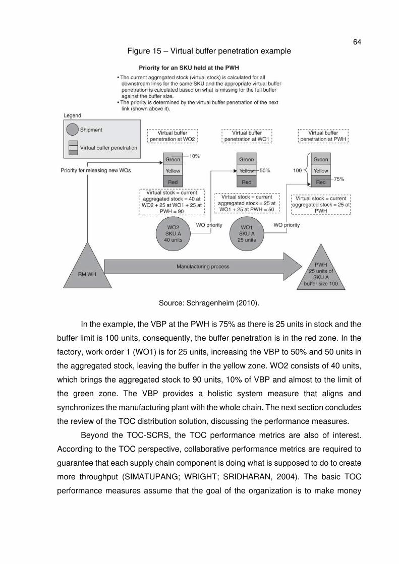
64 Figure 15 – Virtual buffer penetration example
Source: Schragenheim (2010).
In the example, the VBP at the PWH is 75% as there is 25 units in stock and the
buffer limit is 100 units, consequently, the buffer penetration is in the red zone. In the
factory, work order 1 (WO1) is for 25 units, increasing the VBP to 50% and 50 units in
the aggregated stock, leaving the buffer in the yellow zone. WO2 consists of 40 units,
which brings the aggregated stock to 90 units, 10% of VBP and almost to the limit of
the green zone. The VBP provides a holistic system measure that aligns and
synchronizes the manufacturing plant with the whole chain. The next section concludes
the review of the TOC distribution solution, discussing the performance measures.
Beyond the TOC-SCRS, the TOC performance metrics are also of interest.
According to the TOC perspective, collaborative performance metrics are required to
guarantee that each supply chain component is doing what is supposed to do to create
more throughput (SIMATUPANG; WRIGHT; SRIDHARAN, 2004). The basic TOC
performance measures assume that the goal of the organization is to make money
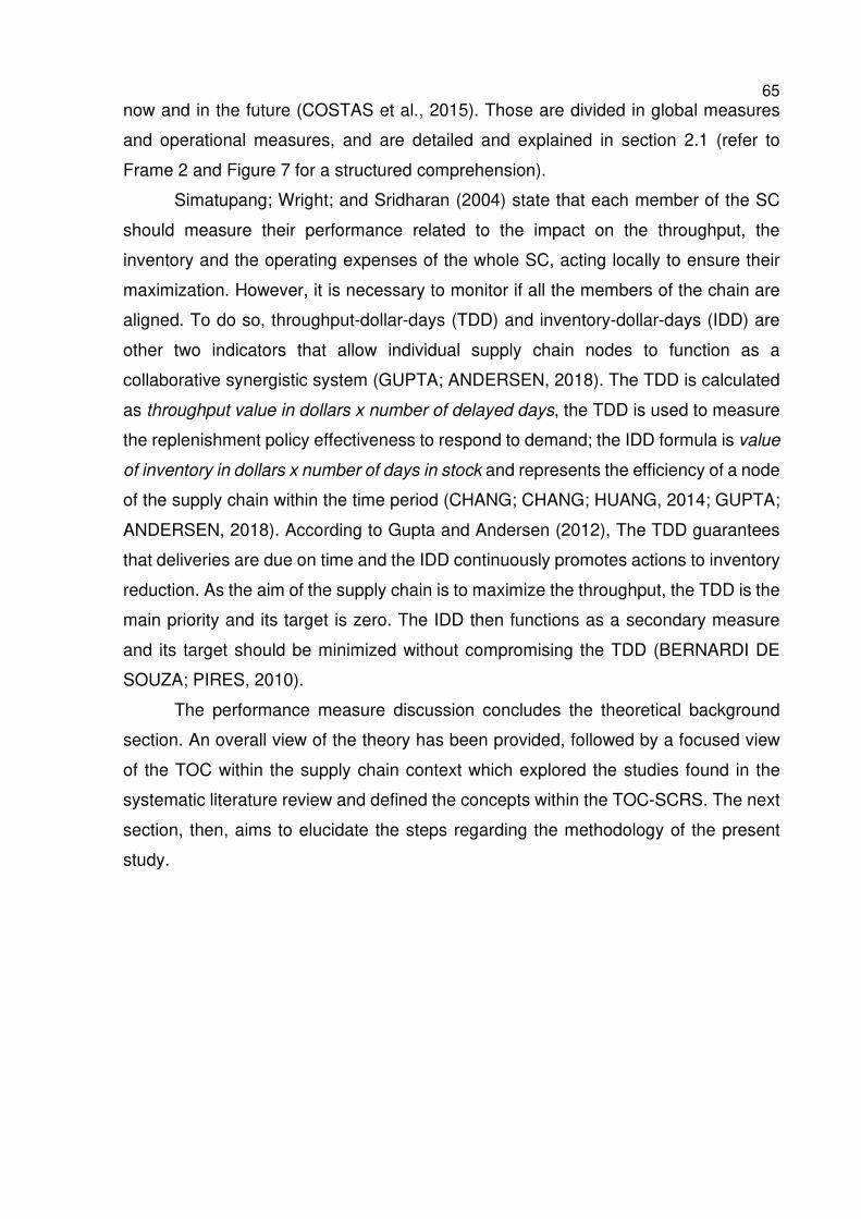
65 now and in the future (COSTAS et al., 2015). Those are divided in global measures
and operational measures, and are detailed and explained in section 2.1 (refer to
Frame 2 and Figure 7 for a structured comprehension).
Simatupang; Wright; and Sridharan (2004) state that each member of the SC
should measure their performance related to the impact on the throughput, the
inventory and the operating expenses of the whole SC, acting locally to ensure their
maximization. However, it is necessary to monitor if all the members of the chain are
aligned. To do so, throughput-dollar-days (TDD) and inventory-dollar-days (IDD) are
other two indicators that allow individual supply chain nodes to function as a
collaborative synergistic system (GUPTA; ANDERSEN, 2018). The TDD is calculated
as throughput value in dollars x number of delayed days, the TDD is used to measure
the replenishment policy effectiveness to respond to demand; the IDD formula is value
of inventory in dollars x number of days in stock and represents the efficiency of a node
of the supply chain within the time period (CHANG; CHANG; HUANG, 2014; GUPTA;
ANDERSEN, 2018). According to Gupta and Andersen (2012), The TDD guarantees
that deliveries are due on time and the IDD continuously promotes actions to inventory
reduction. As the aim of the supply chain is to maximize the throughput, the TDD is the
main priority and its target is zero. The IDD then functions as a secondary measure
and its target should be minimized without compromising the TDD (BERNARDI DE
SOUZA; PIRES, 2010).
The performance measure discussion concludes the theoretical background
section. An overall view of the theory has been provided, followed by a focused view
of the TOC within the supply chain context which explored the studies found in the
systematic literature review and defined the concepts within the TOC-SCRS. The next
section, then, aims to elucidate the steps regarding the methodology of the present
study.
66 3 METHODOLOGICAL PROCEDURES
There are two factors that are essential in conducting successful research: rigor
and relevance (DRESCH; LACERDA; ANTUNES JR., 2015). In that sense, the
introduction section aimed to present the theme and the current scenario of the
research clarifying its relevance. Consecutively, the Methodology section aims to
delineate the research’s rigor defining both research and work methodologies.
Therefore, this section is unfolded in the Research Methodology and Work
Methodology sub-sections.
3.1 RESEARCH METHODOLOGY
In order to ensure the reliability of the results of a research work, especially
scientific research, the researcher must follow a defined procedure or sequence of
steps (DRESCH; LACERDA; ANTUNES JR., 2015). Therefore, to illustrate those steps
and its interdependencies Dresch, Lacerda and Antunes Jr. (2015) represent scientific
research steps through the Newtown’s Pendulum, as can be seen in Figure 16
Figure 16 – Pendulum for carrying out scientific research
Source: Dresch, Lacerda and Antunes Jr. (2015).
67 Having defined the reasons behind this study and its objectives, as presented
in the Introduction Section, it is necessary to define its scientific methods. According to
Saunders; Lewis and Thornhill (2012), there are three main research approaches:
deductive, inductive and abductive. The laws and theories that form scientific
knowledge are derived by induction based on experiments and observation
(CHALMERS, 2013). Once this general knowledge is available it can be utilized to
create predictions and explanation to certain phenomena, which constitutes the
deductive process (CHALMERS, 2013). Lastly, the abduction process makes usage of
data to explore a phenomenon and create a new or alter an existing theory, being
tested subsequently based on new data collection (SAUNDERS; LEWIS; THORNHILL,
2012a). Therefore, this work utilizes mainly the deductive and abductive methods. The
deductive process appears in the construction of the conceptual model and in the
application of the TOC premises in the studied case. Meanwhile, the abductive process
is shown from the exploration of the different proposed scenarios by the case and by
the theory to be tested.
Following the steps to carry out scientific research, after the scientific method
delineation the next step comprises the research methods. According to Dresch,
Lacerda and Antunes Jr. (2015), it is important to define and justify the research
method to ensure that the investigation provides a reasonable answer to the defined
problem. The proper utilization of a research method supports the recognition of the
study by the scientific community, providing evidence that the work is reliable and valid
for the body of knowledge (DRESCH; LACERDA; ANTUNES, 2015). Given the aim of
this work and the complex scenario of the studied case, modeling presents itself as a
sound research method as it allows for better comprehension of complex problems
(PIDD, 2003). Additionally, through computational simulation it is possible to address,
in an exploratory way, complex problem situations where frequent transformation
occurs (PIDD, 2003). Pidd (2003), also points out that computational simulation allows
to find reasonable answers quickly and relative low costs when compared to real world
experimentation. Systems dynamics is then proposed as a simulation tool for the
representation of complex systems, which allows to find better ways to operate this
defined system and comprehend the consequences of the changes (PIDD, 2003).
The quantitative modeling serves as a base for Operational Research
(BERTRAND; FRANSOO, 2002). According to Bertrand and Fransoo (2002), within
68 the OR universe, quantitative modeling research can be classified as empirical or
axiomatic and as descriptive or normative. The axiomatic research aims to find
solutions that provide insights about the problem structure, while the empirical
research intends to find adequacy among between the observations and actions
applied in the real world and the ones applied in the model. Additionally, the normative
research has its interests in developing policies, strategies and actions that improve
the results found in the literature, while the descriptive research analyzes a model that
leads to the comprehension and explanation of the characteristics of the model itself
(BERTRAND; FRANSOO, 2002). In that sense, this research can be classified as
empirical-normative. Having delineated the research method, next section presents
and explains the work methodology.
3.2 WORK METHODOLOGY
The work method, presented in a logical and structured format, is important to
ensure the replicability of the study (MENTZER; FLINT, 1997). The work method
should be constituted by a sequence of logical steps to reach the research’s goals,
ensuring clarity and transparency throughout the process (DRESCH; LACERDA;
ANTUNES JR., 2015). The proposed work method for this work is based on the studies
of Mitroff et al. (1974) and Towill (1993a). Both methods are similar and are presented
comparatively in Figure 17.
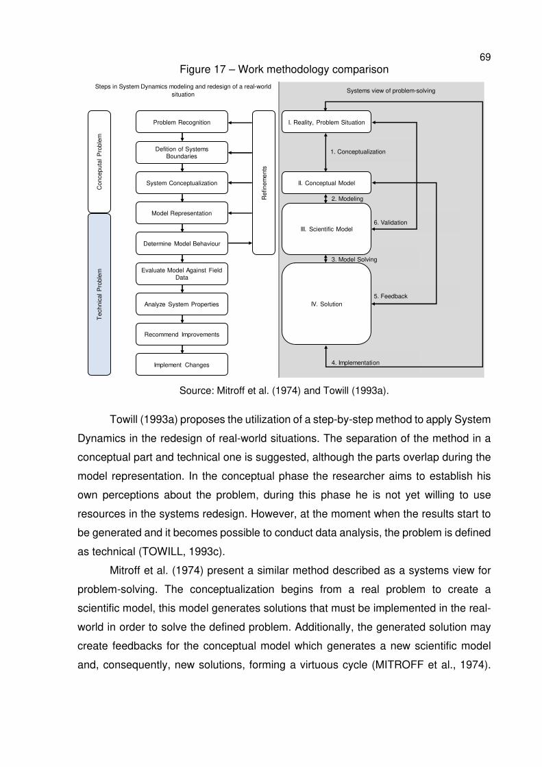
69 Figure 17 – Work methodology comparison
Source: Mitroff et al. (1974) and Towill (1993a).
Towill (1993a) proposes the utilization of a step-by-step method to apply System
Dynamics in the redesign of real-world situations. The separation of the method in a
conceptual part and technical one is suggested, although the parts overlap during the
model representation. In the conceptual phase the researcher aims to establish his
own perceptions about the problem, during this phase he is not yet willing to use
resources in the systems redesign. However, at the moment when the results start to
be generated and it becomes possible to conduct data analysis, the problem is defined
as technical (TOWILL, 1993c).
Mitroff et al. (1974) present a similar method described as a systems view for
problem-solving. The conceptualization begins from a real problem to create a
scientific model, this model generates solutions that must be implemented in the real-
world in order to solve the defined problem. Additionally, the generated solution may
create feedbacks for the conceptual model which generates a new scientific model
and, consequently, new solutions, forming a virtuous cycle (MITROFF et al., 1974).
Steps in System Dynamics modeling and redesign of a real-world situation
Systems view of problem-solving
6. Validation
5. Feedback
4. Implementation
3. Model Solving
2. Modeling
Evaluate Model Against Field Data
Problem Recognition
Defition of Systems Boundaries
System Conceptualization
Determine Model Behaviour
Analyze System Properties
Recommend Improvements
Model Representation
Implement Changes
Ref
inem
ents
Con
cepu
tal
Pro
blem
Tec
hnic
al P
robl
em
I. Reality, Problem Situation
II. Conceptual Model
1. Conceptualization
III. Scientific Model
IV. Solution
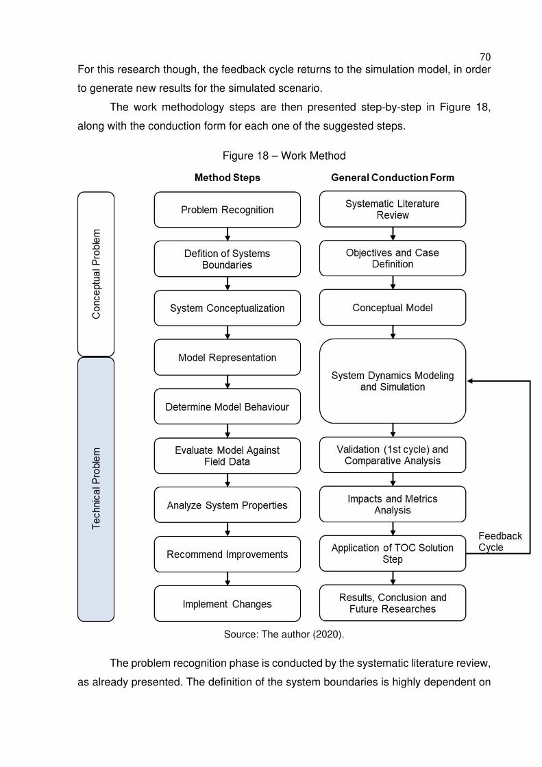
70 For this research though, the feedback cycle returns to the simulation model, in order
to generate new results for the simulated scenario.
The work methodology steps are then presented step-by-step in Figure 18,
along with the conduction form for each one of the suggested steps.
Figure 18 – Work Method
Source: The author (2020).
The problem recognition phase is conducted by the systematic literature review,
as already presented. The definition of the system boundaries is highly dependent on
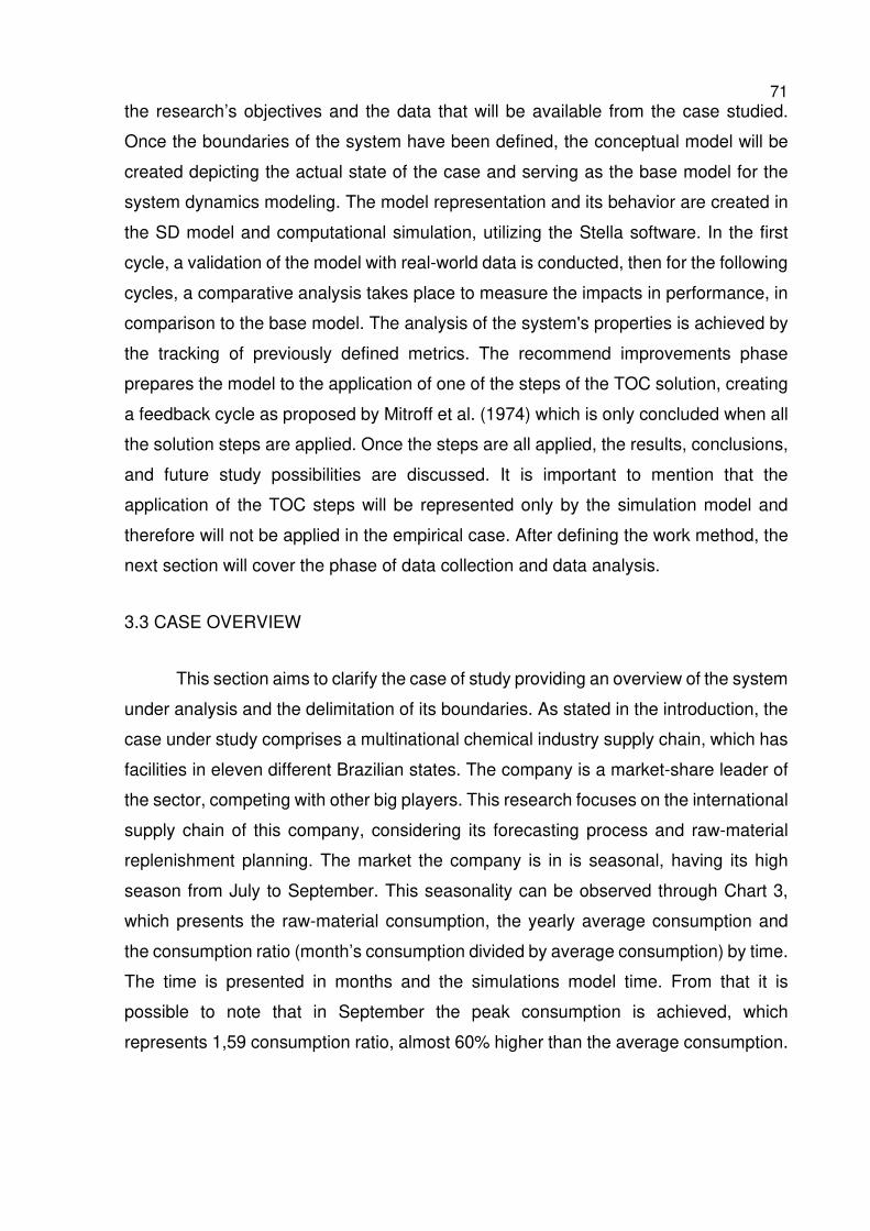
71 the research’s objectives and the data that will be available from the case studied.
Once the boundaries of the system have been defined, the conceptual model will be
created depicting the actual state of the case and serving as the base model for the
system dynamics modeling. The model representation and its behavior are created in
the SD model and computational simulation, utilizing the Stella software. In the first
cycle, a validation of the model with real-world data is conducted, then for the following
cycles, a comparative analysis takes place to measure the impacts in performance, in
comparison to the base model. The analysis of the system's properties is achieved by
the tracking of previously defined metrics. The recommend improvements phase
prepares the model to the application of one of the steps of the TOC solution, creating
a feedback cycle as proposed by Mitroff et al. (1974) which is only concluded when all
the solution steps are applied. Once the steps are all applied, the results, conclusions,
and future study possibilities are discussed. It is important to mention that the
application of the TOC steps will be represented only by the simulation model and
therefore will not be applied in the empirical case. After defining the work method, the
next section will cover the phase of data collection and data analysis.
3.3 CASE OVERVIEW
This section aims to clarify the case of study providing an overview of the system
under analysis and the delimitation of its boundaries. As stated in the introduction, the
case under study comprises a multinational chemical industry supply chain, which has
facilities in eleven different Brazilian states. The company is a market-share leader of
the sector, competing with other big players. This research focuses on the international
supply chain of this company, considering its forecasting process and raw-material
replenishment planning. The market the company is in is seasonal, having its high
season from July to September. This seasonality can be observed through Chart 3,
which presents the raw-material consumption, the yearly average consumption and
the consumption ratio (month’s consumption divided by average consumption) by time.
The time is presented in months and the simulations model time. From that it is
possible to note that in September the peak consumption is achieved, which
represents 1,59 consumption ratio, almost 60% higher than the average consumption.
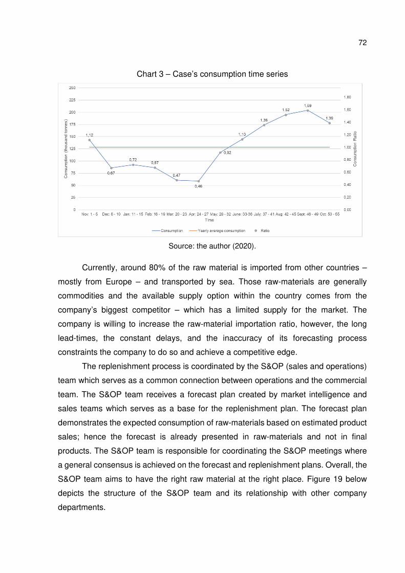
72
Chart 3 – Case’s consumption time series
Source: the author (2020).
Currently, around 80% of the raw material is imported from other countries –
mostly from Europe – and transported by sea. Those raw-materials are generally
commodities and the available supply option within the country comes from the
company’s biggest competitor – which has a limited supply for the market. The
company is willing to increase the raw-material importation ratio, however, the long
lead-times, the constant delays, and the inaccuracy of its forecasting process
constraints the company to do so and achieve a competitive edge.
The replenishment process is coordinated by the S&OP (sales and operations)
team which serves as a common connection between operations and the commercial
team. The S&OP team receives a forecast plan created by market intelligence and
sales teams which serves as a base for the replenishment plan. The forecast plan
demonstrates the expected consumption of raw-materials based on estimated product
sales; hence the forecast is already presented in raw-materials and not in final
products. The S&OP team is responsible for coordinating the S&OP meetings where
a general consensus is achieved on the forecast and replenishment plans. Overall, the
S&OP team aims to have the right raw material at the right place. Figure 19 below
depicts the structure of the S&OP team and its relationship with other company
departments.
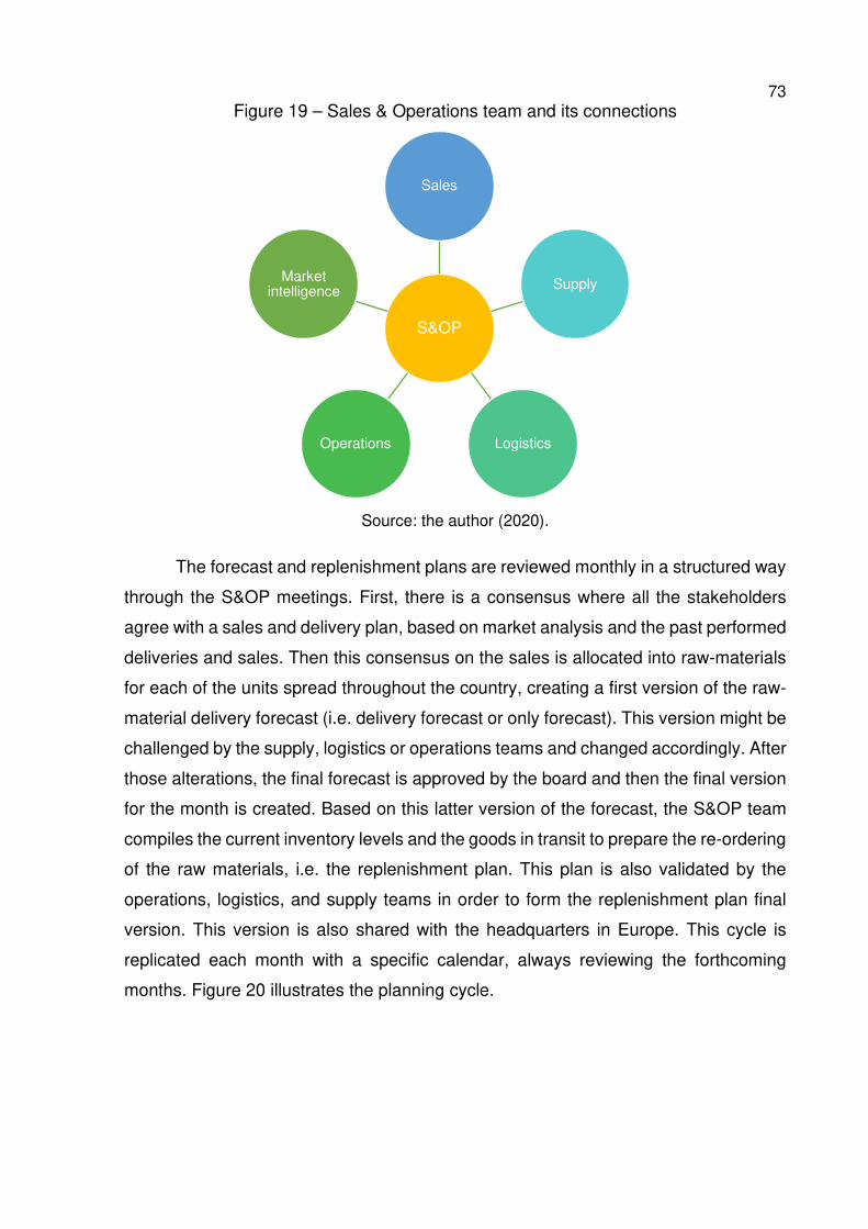
73 Figure 19 – Sales & Operations team and its connections
Source: the author (2020).
The forecast and replenishment plans are reviewed monthly in a structured way
through the S&OP meetings. First, there is a consensus where all the stakeholders
agree with a sales and delivery plan, based on market analysis and the past performed
deliveries and sales. Then this consensus on the sales is allocated into raw-materials
for each of the units spread throughout the country, creating a first version of the raw-
material delivery forecast (i.e. delivery forecast or only forecast). This version might be
challenged by the supply, logistics or operations teams and changed accordingly. After
those alterations, the final forecast is approved by the board and then the final version
for the month is created. Based on this latter version of the forecast, the S&OP team
compiles the current inventory levels and the goods in transit to prepare the re-ordering
of the raw materials, i.e. the replenishment plan. This plan is also validated by the
operations, logistics, and supply teams in order to form the replenishment plan final
version. This version is also shared with the headquarters in Europe. This cycle is
replicated each month with a specific calendar, always reviewing the forthcoming
months. Figure 20 illustrates the planning cycle.
S&OP
Sales
Supply
LogisticsOperations
Market intelligence
74 Figure 20 – Forecast and planning cycle
Source: the author (2020).
The forecast and replenishment plan are conducted for all the units in the
country. The unit's management is divided between production (total of five) and mixing
units (total of 24). The mixing units are then divided again into three other management
structures according to their regional location. For this research, the focus will be on
the Rio Grande do Sul state units given its representativeness in sales for the whole
company. The state is the company’s most representative state, accounting for 28%
of the total sales volume, while the second greatest state has approximately 17%, the
third 15%, and other 9 states the remaining 39%. There are four units in the state
located in four different cities, being one of them a production unit with its own seaport
– referred as RIG – and the other three being mixing units – referred as CAN, CZB,
and POA. Usually, the seaport unit transfers raw materials to the mixing units, although
depending on the material, some mixing units might receive the material directly from
a supplier and transfer to any other requesting unit. During a one-year period, around
780 thousands of tonnes were transferred between those four units. Figure 21 provides
an overall view of the described system that aids in the understanding of the case’s
supply chain.
Overall consensus
Allocation of raw materials by unit
Forecast first draft
Forecast changes
Board approval
Raw material forecast
Data compilation
Replenishment plan validation
Replenishment plan
International headquarters
report
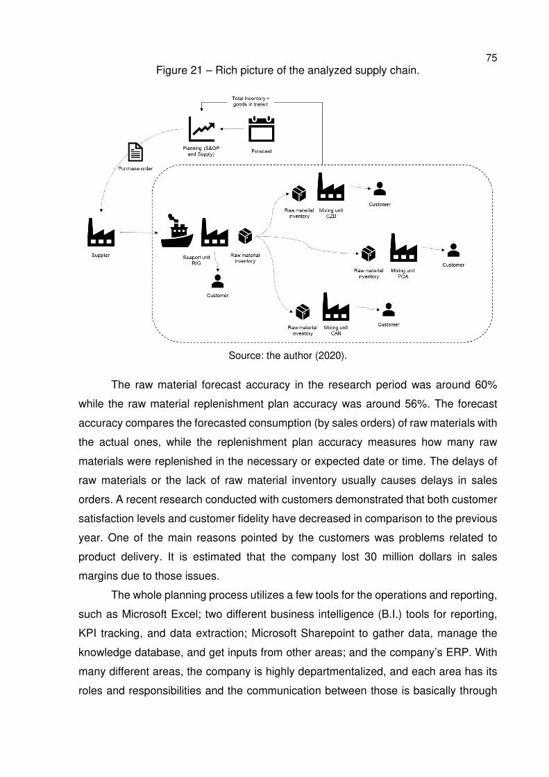
75 Figure 21 – Rich picture of the analyzed supply chain.
Source: the author (2020).
The raw material forecast accuracy in the research period was around 60%
while the raw material replenishment plan accuracy was around 56%. The forecast
accuracy compares the forecasted consumption (by sales orders) of raw materials with
the actual ones, while the replenishment plan accuracy measures how many raw
materials were replenished in the necessary or expected date or time. The delays of
raw materials or the lack of raw material inventory usually causes delays in sales
orders. A recent research conducted with customers demonstrated that both customer
satisfaction levels and customer fidelity have decreased in comparison to the previous
year. One of the main reasons pointed by the customers was problems related to
product delivery. It is estimated that the company lost 30 million dollars in sales
margins due to those issues.
The whole planning process utilizes a few tools for the operations and reporting,
such as Microsoft Excel; two different business intelligence (B.I.) tools for reporting,
KPI tracking, and data extraction; Microsoft Sharepoint to gather data, manage the
knowledge database, and get inputs from other areas; and the company’s ERP. With
many different areas, the company is highly departmentalized, and each area has its
roles and responsibilities and the communication between those is basically through
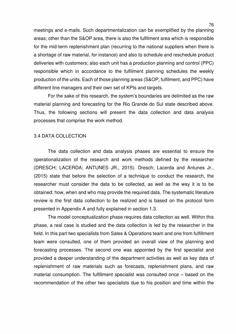
76 meetings and e-mails. Such departmentalization can be exemplified by the planning
areas; other than the S&OP area, there is also the fulfilment area which is responsible
for the mid-term replenishment plan (recurring to the national suppliers when there is
a shortage of raw material, for instance) and also to schedule and reschedule product
deliveries with customers; also each unit has a production planning and control (PPC)
responsible which in accordance to the fulfilment planning schedules the weekly
production of the units. Each of those planning areas (S&OP, fulfilment, and PPC) have
different line managers and their own set of KPIs and targets.
For the sake of this research, the system’s boundaries are delimited as the raw
material planning and forecasting for the Rio Grande do Sul state described above.
Thus, the following sections will present the data collection and data analysis
processes that comprise the work method.
3.4 DATA COLLECTION
The data collection and data analysis phases are essential to ensure the
operationalization of the research and work methods defined by the researcher
(DRESCH; LACERDA; ANTUNES JR., 2015). Dresch; Lacerda and Antunes Jr.,
(2015) state that before the selection of a technique to conduct the research, the
researcher must consider the data to be collected, as well as the way it is to be
obtained: how, when and who may provide the required data. The systematic literature
review is the first data collection to be realized and is based on the protocol form
presented in Appendix A and fully explained in section 1.3.
The model conceptualization phase requires data collection as well. Within this
phase, a real case is studied and the data collection is led by the researcher in the
field. In this part two specialists from Sales & Operations team and one from fulfillment
team were consulted, one of them provided an overall view of the planning and
forecasting processes. The second one was appointed by the first specialist and
provided a deeper understanding of the department activities as well as key data of
replenishment of raw materials such as forecasts, replenishment plans, and raw
material consumption. The fulfillment specialist was consulted once – based on the
recommendation of the other two specialists due to his position and time within the
77 company – in order to provide data on the sales order deliveries and delays. The
consulted specialists and their profiles are presented in the frame below.
Frame 6 – Company’s specialists consulted
Position Company
time Education background
Senior S&OP coordinator 9 years Business administration at Unisinos University
S&OP coordinator 10 years Production engineering at Federal University of Rio
Grande do Sul
Fulfillment coordinator 9 years Chemical engineering at Federal University of Rio
Grande
Source: the author (2020).
Ideally, all the data from production and raw material planning would be
supported by sales data and the delays would be accounted in the sales orders.
However, during data collection it was noted that the company does not have a good
record of the sales orders delays. Two problems emerged regarding the sales orders
dates of delivery. The first one is that the initial date at the sales order is commonly not
relevant as the customer does not yet have a specific date to receive the products. The
sales orders can be created even six months prior to the delivery date; therefore, the
sales teams usually provide an irrelevant delivery date. Later, the fulfillment team
contacts the customers to agree on an expected delivery date. As raw materials delays
occur consequently changing to the sales orders delivery plan the fulfillment team
contacts the costumer again to negotiate a new delivery date. All those changes in
delivery date are not registered, the only record kept is the most recent delivery date
meaning that at each interaction the former delivery date is lost. Therefore, the initial
delivery date inputted in the system is not accurate and all the further changes to those
delivery dates are lost, so delivery delays are difficult to track. In that sense the data
collection and the model limit itself to consider only the raw material supply and
replenishment systems, not accounting the sales operations.
The sources of data are varied. The second specialist provided various
spreadsheets from the S&OP, supply, and logistics teams, access to those teams’
knowledge databases – company’s teams websites found in the intranet – and their
business intelligence (B.I.) pages. Additionally, the company’s ERP was also
consulted. Therefore, data sources are the company’s ERP database, logistics, S&OP,
78 and supply department data, as well as the direct observation of the researcher. This
information was then compiled and followed by another two interviews with the
company’s S&OP specialists to come to a consensus of the structured data and the
conceptual model validation. The data collection is then composed of five different
techniques, respectively bibliographic, documentary, direct observation, and
interviews (SAUNDERS; LEWIS; THORNHILL, 2012b). The frame below presents the
variables collected, a brief description of them and their sources.
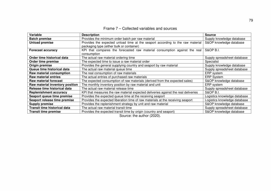
79
Frame 7 – Collected variables and sources
Variable Description Source Batch premise Provides the minimum order batch per raw material Supply knowledge database Unload premise Provides the expected unload time at the seaport according to the raw material
packaging type (either bulk or container) S&OP knowledge database
Forecast accuracy KPI that compares the forecasted raw material consumption against the real consumption
S&OP B.I.
Order time historical data The actual raw material ordering time Supply spreadsheet database Order time premise The expected time to issue a raw material order Specialist Origin premise Provides the general supplying country and seaport by raw material Supply knowledge database Queue time historical data The actual raw material queue time Supply spreadsheet database Raw material consumption The real consumption of raw materials ERP system Raw material entries The actual entries of purchased raw materials ERP System Raw material forecast The expected consumption of raw materials (derived from the expected sales) S&OP knowledge database Raw material inventory position The monthly inventory position by raw material and unit ERP system Release time historical data The actual raw material release time Supply spreadsheet database Replenishment accuracy KPI that measures the raw material expected deliveries against the real deliveries S&OP B.I. Seaport queue time premise Provides the expected queue time at the receiving seaport Logistics knowledge database Seaport release time premise Provides the expected liberation time of raw materials at the receiving seaport Logistics knowledge database Supply premise Provides the replenishment strategy by unit and raw material S&OP knowledge database Transit time historical data The actual raw material transit time Supply spreadsheet database Transit time premise Provides the expected transit time by origin (country and seaport) S&OP knowledge database
Source: the author (2020).
80 The variables above are used in order to construct the system dynamics model.
All the time-varying variables (raw material forecast, consumption, inventory positions,
and time historical data) had a dataset of one year, ranging from the 1st of November
2018 to 31st October 2019. As stated, this research aims to simulate four plants of the
mentioned company, therefore all the data collected regarded only those plants. The
seaport unit is referred to as RIG, while the other three mixing units can be referred to
as CAN, POA, and CZB. A total of 29 different raw materials are imported for those
units and 28 will be part of this research1. Having detailed the data collection, the next
section covers the data analysis of the research.
3.5 DATA ANALYSIS
The data analysis can be defined as the phase where the researcher interprets
the collected data to find the results of the study (DRESCH; LACERDA; ANTUNES
JR., 2015). In the problem recognition and the definition of the system boundaries
content analysis is utilized derived from the systematic literature review. From the data
generated from the documents, observations and the interviews follow a content
analysis of those, in order to conceptualize the system, represent the model and define
its behaviors. This data is then inputted in a conceptual model without randomness for
the verification phase. The verification is suggested by Sterman (2000) and aims to
verify if the model behaves as the real system does. Next, randomness is added in the
model by the cumulative probability distributions derived from the real data of the lead
times – please refer to Appendices F, G, and H for those distributions. Those
distributions are coded directly in Stella built-in functions. For the model validation,
confidence intervals of the average inventory position are defined using Stella’s
sensitivity analysis with multiple runs and compared with the real data found in the data
collection. For those a significance level of 5% is used and the maximum error allowed
is set to 10% based on the real case values. A t test is conducted to verify that the
number of runs in the sensitivity analysis is enough. The validation process is detailed
later in the model section.
1 One specific raw material had to be excluded from the analysis as a suggestion of the S&OP specialist due to reporting inconsistencies between the forecast data, the ERP consumption information, and the supply data.
81 Once the model is validated, the TOC solution steps are applied in a logical
sequence and the results are recorded for each one of those iterations. In order to
evaluate the results from the TOC application the total inventory, inventory at the
mixing units, inventory at the seaport unit, the throughput-dollar-days (TDD), and the
inventory-dollar-days (IDD) are monitored. Regarding the unit of measurement, both
TDD and IDD are in dollars and the inventories in tonnes.
As specified in the data collection section, since there is no accurate control of
the sales orders delays, a proxy variable is utilized to account for the TDD. A proxy is
a variable that is used to replace an unmeasurable or unobservable variable, although
not a direct measure of the desired variable, a good proxy is strongly related to the
variable of interest (LEWIS-BECK; BRYMAN; FUTING LIAO, 2004). Based on the
specialists a good proxy for the sales orders delays is the raw material delays. Since
the company has a make-to-order production system, any unexpected delay of raw
materials can cause a direct delay in sales.
In order to evaluate the impacts of the TOC, at each iteration of the application
of the distribution solution steps the results of the mentioned variables are be computed
and compared to the previous result and the base model. The interest variables are
defined as the throughput-dollar-days (TDD), the inventory-dollar-days (IDD), the
inventory levels (at the CWH, at the shops, and at the whole SC). With the model
results first, descriptive statistics are presented, both for the base model and the
implementation of the steps. Then, a Shapiro-Wilk test (SHAPIRO; WILK, 1965) is
conducted to check for data normality. The results show non-normal distributions.
Therefore, the Kruskal-Wallis test is realized to check if there is any significative
change between the scenarios. Since the Kruskal-Wallis test only informs that at least
one of the scenarios is different, not indicating which are the different ones, the
analysis is complemented with the Hochberg test (HOCHBERG, 1988). This test is
utilized for multiple scenario comparison, providing the pairwise significances at each
combination between the observed groups. Those groups are represented in the case
by the base model and the created scenarios that apply the TOC’s steps.
Finally, causal impact analysis – as proposed by (BRODERSEN et al., 2015) –
is utilized to analyze the system properties and recommend improvements. According
to Brodersen et al (2015), a causal inference may be understood as intervention or
data treatment realized in a temporal series. The causal impact is the difference
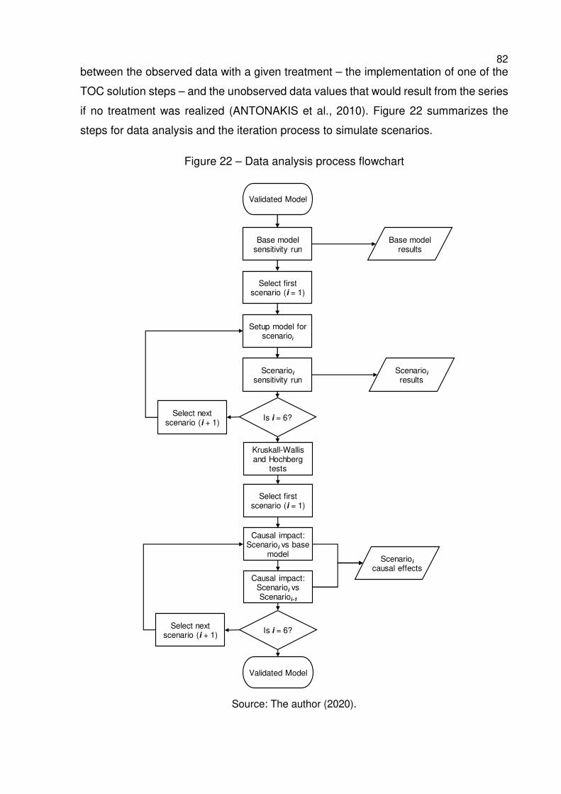
82 between the observed data with a given treatment – the implementation of one of the
TOC solution steps – and the unobserved data values that would result from the series
if no treatment was realized (ANTONAKIS et al., 2010). Figure 22 summarizes the
steps for data analysis and the iteration process to simulate scenarios.
Figure 22 – Data analysis process flowchart
Source: The author (2020).
Validated Model
Base model sensitivity run
Base model results
Setup model for scenarioi
Scenarioi
sensitivity runScenarioi
results
Kruskall-Wallisand Hochberg
tests
Is i = 6?Select next scenario (i + 1)
Select first scenario (i = 1)
Causal impact: Scenarioi vs base
model
Causal impact: Scenarioi vs Scenarioi-1
Select first scenario (i = 1)
Is i = 6?Select next scenario (i + 1)
Scenarioi
causal effects
Validated Model
83 The scenarios defined for the analyses are shown in Frame 8. From the frame,
it is possible to note which TOC steps are being applied, which model variables are
used or not, and whether the buffer if based on the forecast (FB) or not (not FB). The
buffer determination and the replenishment lead time are separated as individual
variables. For those scenarios, the sensitivity runs are conducted with 30 multiple runs
per simulation, resulting in a total of 210 simulation runs. The results for each scenario
were exported to an Excel file and R was used in order to organize, summarize, and
structure the results data for analysis.
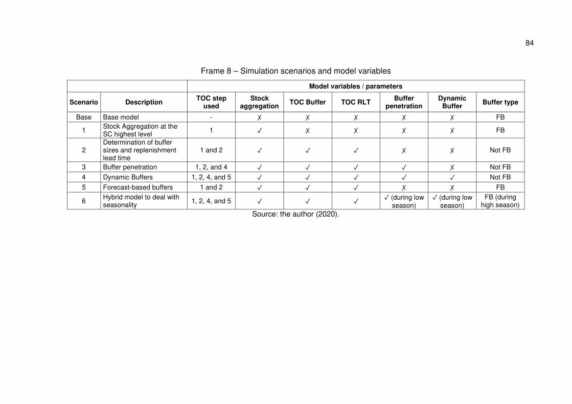
84
Frame 8 – Simulation scenarios and model variables
Model variables / parameters
Scenario Description TOC step
used Stock
aggregation TOC Buffer TOC RLT
Buffer penetration
Dynamic Buffer
Buffer type
Base Base model - ✗ ✗ ✗ ✗ ✗ FB
1 Stock Aggregation at the SC highest level 1 ✓ ✗ ✗ ✗ ✗ FB
2 Determination of buffer sizes and replenishment lead time
1 and 2 ✓ ✓ ✓ ✗ ✗ Not FB
3 Buffer penetration 1, 2, and 4 ✓ ✓ ✓ ✓ ✗ Not FB
4 Dynamic Buffers 1, 2, 4, and 5 ✓ ✓ ✓ ✓ ✓ Not FB
5 Forecast-based buffers 1 and 2 ✓ ✓ ✓ ✗ ✗ FB
6 Hybrid model to deal with seasonality 1, 2, 4, and 5 ✓ ✓ ✓
✓ (during low season)
✓ (during low season)
FB (during high season)
Source: the author (2020).
85
Also, it is important to mention that there was no expected disturbance on the
demand, capacity expansion, significative technological improvement, or any other
impactful initiative during the data colletion. The data analysis concludes the
methodological procedures. The next section describes and details the model
construction.
86 4 MODEL CONSTRUCTION
In this section, the construction process of the system dynamics model is
described. For the model construction, the four units are created as well as the
variables such as the raw material replenishment, the raw material consumption, and
the transfers between the units. Initially, all the data collected serves as a direct input
to the model, so no randomness is yet set. This step is conducted to verify the model
behavior, which is done by comparing the final inventory position of the raw materials
in the systems against the real data found in the company’s ERP. Later, the planning
process module of the system is created, which aims to simulate the forecasting and
replenishment process of the company. During this phase, variation is added to the
model through the lead times, based on the cumulative distribution function of the
historical supply data, thus creating the base model. Finally, the base model is
validated in Stella utilizing the confidence intervals of the average inventory of raw
materials and comparing those to the real data.
The TOC steps application are created in the model as parameters, therefore in
order to run a simulation with or without a specific TOC step is just a matter of adjusting
the respective parameters. Therefore, the same model is utilized for the base model
and all of the necessary scenarios are simulated by adjusting the respective
parameters, assuring replicability of the base values or any required scenario at any
moment.
The next section covers the conceptualization of system, the creation of the
internal supply chain module and the initial model verification.
4.1 SYSTEM CONCEPTUALIZATION
As previously stated, the model will simulate the planning and replenishment of
raw material of four units. The biggest unit is a production unit that has its own seaport,
while the other ones are mixing units. The seaport unit is referred to as RIG, while the
other three mixing units can be referred to as CAN, POA, and CZB. The raw material
forecast starts the whole planning process. This forecast demonstrates the expected
consumptions in tonnes for at least the next six months and is detailed by raw material
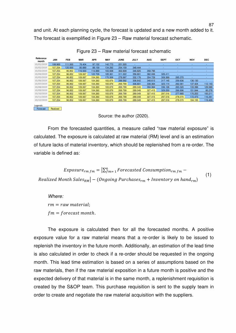
87 and unit. At each planning cycle, the forecast is updated and a new month added to it.
The forecast is exemplified in Figure 23 – Raw material forecast schematic.
Figure 23 – Raw material forecast schematic
Source: the author (2020).
From the forecasted quantities, a measure called “raw material exposure” is
calculated. The exposure is calculated at raw material (RM) level and is an estimation
of future lacks of material inventory, which should be replenished from a re-order. The
variable is defined as:
�������� � = �∑ ���������� ����������� ���� � −
�������� ���ℎ "����#$� − (&�'���' (���ℎ���� + *�+�����, �� ℎ���) (1)
Where:
�� = ��- ��������;
/� = /������� ����ℎ.
The exposure is calculated then for all the forecasted months. A positive
exposure value for a raw material means that a re-order is likely to be issued to
replenish the inventory in the future month. Additionally, an estimation of the lead time
is also calculated in order to check if a re-order should be requested in the ongoing
month. This lead time estimation is based on a series of assumptions based on the
raw materials, then if the raw material exposition in a future month is positive and the
expected delivery of that material is in the same month, a replenishment requisition is
created by the S&OP team. This purchase requisition is sent to the supply team in
order to create and negotiate the raw material acquisition with the suppliers.
Reference
monthJAN FEB MAR APR MAY JUNE JULY AUG SEPT OCT NOV DEC
01/01/2019 108.900 111.500 76.404 97.132 142.773 221.520 - - - - - -01/02/2019 107.254 120.500 80.889 88.159 134.292 254.159 348.444 - - - - -01/03/2019 107.254 96.852 116.500 114.889 183.938 302.609 346.825 358.795 - - - -01/04/2019 107.254 96.852 109.067 122.726 185.361 311.022 356.801 382.006 326.411 - - -01/05/2019 107.254 96.852 109.067 104.260 170.306 278.997 332.176 354.729 309.369 265.370 - -01/06/2019 107.254 96.852 109.067 104.260 183.879 288.592 306.642 348.613 317.145 259.836 136.130 -01/07/2019 107.254 96.852 109.067 104.260 183.879 269.799 306.801 338.364 323.114 262.061 137.424 112.143 01/08/2019 107.254 96.852 109.067 104.260 183.879 269.799 289.049 350.364 336.126 263.320 133.396 129.589 01/09/2019 107.254 96.852 109.067 104.260 183.879 269.799 289.049 327.415 329.250 266.896 151.844 85.278 01/10/2019 107.254 96.852 109.067 104.260 183.879 269.799 289.049 327.415 297.516 277.665 170.253 100.211 01/11/2019 107.254 96.852 109.067 104.260 183.879 269.799 289.049 327.415 297.516 278.070 172.473 116.261 01/12/2019 107.254 96.852 109.067 104.260 183.879 269.799 289.049 327.415 297.516 278.070 184.195 119.409
Legends:
Forecast Realized
88 The first premise to calculate the expected lead time is the supply premise. This
premise defines for each raw material its supplying unit, i.e. the unit that is responsible
for supplying that material to other units when necessary. Since RIG has its own
seaport and is the biggest unit of the region, most materials are supplied through this
unit. However, other plants can be suppliers of a few materials as well, even though
they necessarily need to arrive first at the RIG seaport. Thus, the plants that are
supplied by the supplying unit need to issue a replenishment order to have the material
transferred and available to them. Since the plants are all within the same state the
transfer lead time is of one week, with little variation as long as the supplying plant has
the inventory in hand. The replenishment frequency does not follow a predefined rule,
and it varies according to the units and the materials, they can be daily depending on
the demand or more sparse. Usually, all units keep extra inventory in their possession.
Summing up, the supply premise defines which unit aggregates the inventory of that
specific raw material. Frame 9 lists the raw materials and how they are supplied. It
shows, for instance, that the raw material DAP GR is supplied by an external supplier
at the RIG unit and then the RIG unit supplies that raw material for the other units.
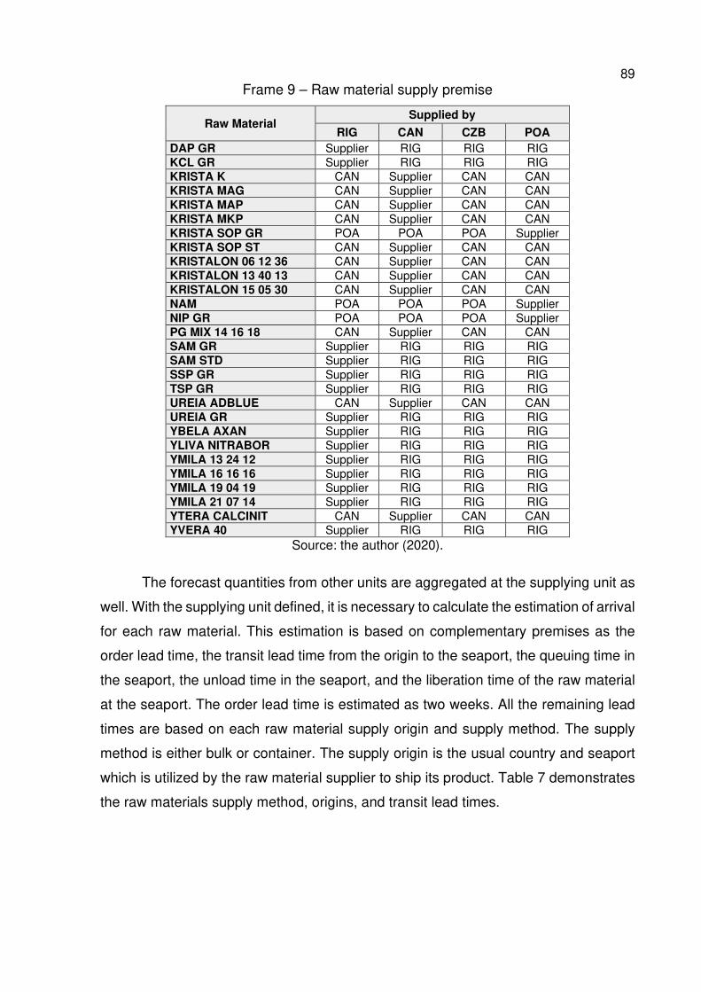
89 Frame 9 – Raw material supply premise
Raw Material Supplied by
RIG CAN CZB POA
DAP GR Supplier RIG RIG RIG KCL GR Supplier RIG RIG RIG KRISTA K CAN Supplier CAN CAN KRISTA MAG CAN Supplier CAN CAN KRISTA MAP CAN Supplier CAN CAN KRISTA MKP CAN Supplier CAN CAN KRISTA SOP GR POA POA POA Supplier KRISTA SOP ST CAN Supplier CAN CAN KRISTALON 06 12 36 CAN Supplier CAN CAN KRISTALON 13 40 13 CAN Supplier CAN CAN KRISTALON 15 05 30 CAN Supplier CAN CAN NAM POA POA POA Supplier NIP GR POA POA POA Supplier PG MIX 14 16 18 CAN Supplier CAN CAN SAM GR Supplier RIG RIG RIG SAM STD Supplier RIG RIG RIG SSP GR Supplier RIG RIG RIG TSP GR Supplier RIG RIG RIG UREIA ADBLUE CAN Supplier CAN CAN UREIA GR Supplier RIG RIG RIG YBELA AXAN Supplier RIG RIG RIG YLIVA NITRABOR Supplier RIG RIG RIG YMILA 13 24 12 Supplier RIG RIG RIG YMILA 16 16 16 Supplier RIG RIG RIG YMILA 19 04 19 Supplier RIG RIG RIG YMILA 21 07 14 Supplier RIG RIG RIG YTERA CALCINIT CAN Supplier CAN CAN YVERA 40 Supplier RIG RIG RIG
Source: the author (2020).
The forecast quantities from other units are aggregated at the supplying unit as
well. With the supplying unit defined, it is necessary to calculate the estimation of arrival
for each raw material. This estimation is based on complementary premises as the
order lead time, the transit lead time from the origin to the seaport, the queuing time in
the seaport, the unload time in the seaport, and the liberation time of the raw material
at the seaport. The order lead time is estimated as two weeks. All the remaining lead
times are based on each raw material supply origin and supply method. The supply
method is either bulk or container. The supply origin is the usual country and seaport
which is utilized by the raw material supplier to ship its product. Table 7 demonstrates
the raw materials supply method, origins, and transit lead times.
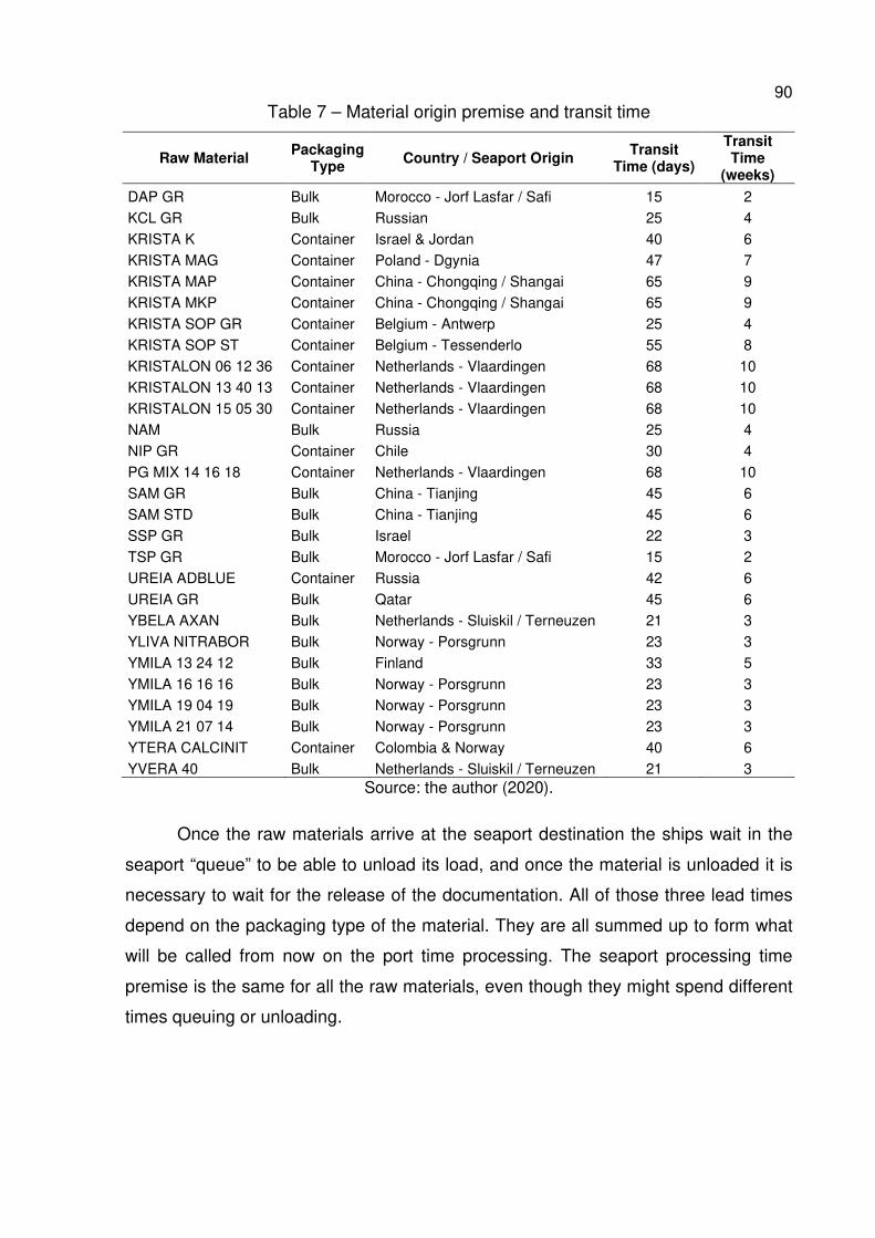
90 Table 7 – Material origin premise and transit time
Raw Material Packaging
Type Country / Seaport Origin
Transit Time (days)
Transit Time
(weeks)
DAP GR Bulk Morocco - Jorf Lasfar / Safi 15 2 KCL GR Bulk Russian 25 4 KRISTA K Container Israel & Jordan 40 6 KRISTA MAG Container Poland - Dgynia 47 7 KRISTA MAP Container China - Chongqing / Shangai 65 9 KRISTA MKP Container China - Chongqing / Shangai 65 9 KRISTA SOP GR Container Belgium - Antwerp 25 4 KRISTA SOP ST Container Belgium - Tessenderlo 55 8 KRISTALON 06 12 36 Container Netherlands - Vlaardingen 68 10 KRISTALON 13 40 13 Container Netherlands - Vlaardingen 68 10 KRISTALON 15 05 30 Container Netherlands - Vlaardingen 68 10 NAM Bulk Russia 25 4 NIP GR Container Chile 30 4 PG MIX 14 16 18 Container Netherlands - Vlaardingen 68 10 SAM GR Bulk China - Tianjing 45 6 SAM STD Bulk China - Tianjing 45 6 SSP GR Bulk Israel 22 3 TSP GR Bulk Morocco - Jorf Lasfar / Safi 15 2 UREIA ADBLUE Container Russia 42 6 UREIA GR Bulk Qatar 45 6 YBELA AXAN Bulk Netherlands - Sluiskil / Terneuzen 21 3 YLIVA NITRABOR Bulk Norway - Porsgrunn 23 3 YMILA 13 24 12 Bulk Finland 33 5 YMILA 16 16 16 Bulk Norway - Porsgrunn 23 3 YMILA 19 04 19 Bulk Norway - Porsgrunn 23 3 YMILA 21 07 14 Bulk Norway - Porsgrunn 23 3 YTERA CALCINIT Container Colombia & Norway 40 6 YVERA 40 Bulk Netherlands - Sluiskil / Terneuzen 21 3
Source: the author (2020).
Once the raw materials arrive at the seaport destination the ships wait in the
seaport “queue” to be able to unload its load, and once the material is unloaded it is
necessary to wait for the release of the documentation. All of those three lead times
depend on the packaging type of the material. They are all summed up to form what
will be called from now on the port time processing. The seaport processing time
premise is the same for all the raw materials, even though they might spend different
times queuing or unloading.
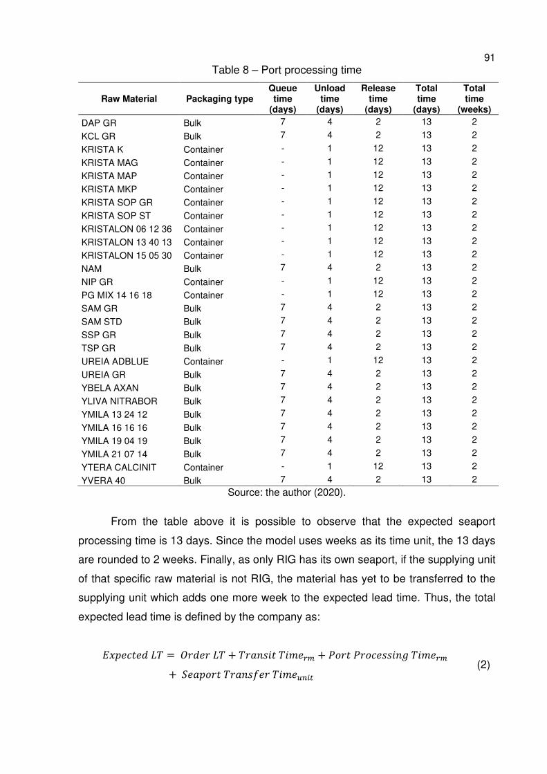
91 Table 8 – Port processing time
Raw Material Packaging type Queue time
(days)
Unload time
(days)
Release time
(days)
Total time
(days)
Total time
(weeks)
DAP GR Bulk 7 4 2 13 2
KCL GR Bulk 7 4 2 13 2
KRISTA K Container - 1 12 13 2
KRISTA MAG Container - 1 12 13 2
KRISTA MAP Container - 1 12 13 2
KRISTA MKP Container - 1 12 13 2
KRISTA SOP GR Container - 1 12 13 2
KRISTA SOP ST Container - 1 12 13 2
KRISTALON 06 12 36 Container - 1 12 13 2
KRISTALON 13 40 13 Container - 1 12 13 2
KRISTALON 15 05 30 Container - 1 12 13 2
NAM Bulk 7 4 2 13 2
NIP GR Container - 1 12 13 2
PG MIX 14 16 18 Container - 1 12 13 2
SAM GR Bulk 7 4 2 13 2
SAM STD Bulk 7 4 2 13 2
SSP GR Bulk 7 4 2 13 2
TSP GR Bulk 7 4 2 13 2
UREIA ADBLUE Container - 1 12 13 2
UREIA GR Bulk 7 4 2 13 2
YBELA AXAN Bulk 7 4 2 13 2
YLIVA NITRABOR Bulk 7 4 2 13 2
YMILA 13 24 12 Bulk 7 4 2 13 2
YMILA 16 16 16 Bulk 7 4 2 13 2
YMILA 19 04 19 Bulk 7 4 2 13 2
YMILA 21 07 14 Bulk 7 4 2 13 2
YTERA CALCINIT Container - 1 12 13 2
YVERA 40 Bulk 7 4 2 13 2 Source: the author (2020).
From the table above it is possible to observe that the expected seaport
processing time is 13 days. Since the model uses weeks as its time unit, the 13 days
are rounded to 2 weeks. Finally, as only RIG has its own seaport, if the supplying unit
of that specific raw material is not RIG, the material has yet to be transferred to the
supplying unit which adds one more week to the expected lead time. Thus, the total
expected lead time is defined by the company as:
�������� 01 = &���� 01 + 1������ 1��� + (��� (��������' 1���
+ "������ 1����/�� 1���2345 (2)
92
Where:
�� = ��- �������� �� ���;
���� = ����������� ����.
Then, as stated previously if the expected lead time is equal to or less than raw
material exposure in the forecasted month a purchase requisition is created for that
material. All those requisitions form the replenishment plan. However, the requisition
quantity is not the same as the raw material exposure, besides the raw material
exposures, it is also necessary to account for the supplying batch sizes as well as an
additional measure of safety. Both are defined for each raw material, while the order
batch is defined by the suppliers – which also affect the minimum batch, as at least
one batch must be procured – the safety measures are defined by the S&OP and
supply teams. The safety measure basically relates to the criticality of the material –
e.g. if it can be found within the country market, how easily it can be replaced, for which
products it is used, etc. – and it consists of three levels. Each level defines an extra
quantity to be purchased for each raw material at each re-order. Level 1 will consider
the forecasted exposure plus the next month’s forecast after the exposure for that
material; level 2 will considerer the exposure plus the next two forecasted months after
the exposure; and level 3, the exposure plus the next three months forecasted
quantities after exposure. A material without the safety factor will only consider the raw
exposure. Even though those levels are generally defined, they may change
depending on the current situation or through time. Table 9 presents the safety factors
and the batch premises (in thousands of tonnes) for each raw material.
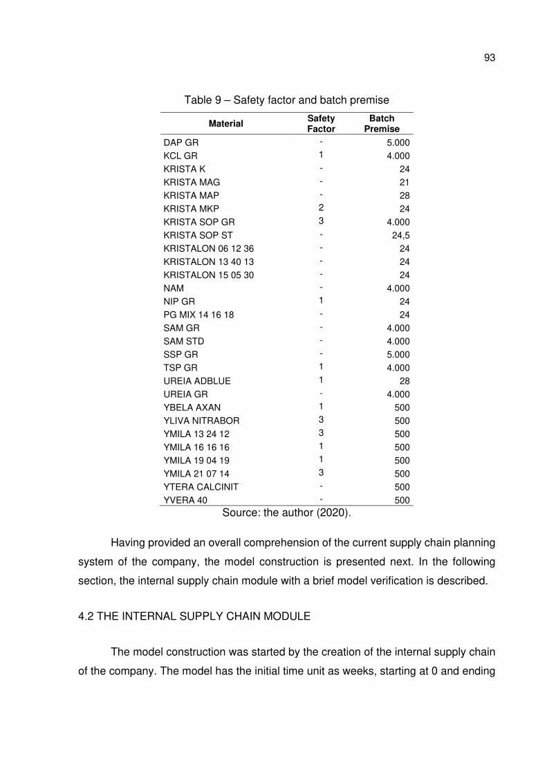
93
Table 9 – Safety factor and batch premise
Material Safety Factor
Batch Premise
DAP GR - 5.000 KCL GR 1 4.000 KRISTA K - 24 KRISTA MAG - 21 KRISTA MAP - 28 KRISTA MKP 2 24 KRISTA SOP GR 3 4.000 KRISTA SOP ST - 24,5 KRISTALON 06 12 36 - 24 KRISTALON 13 40 13 - 24 KRISTALON 15 05 30 - 24 NAM - 4.000 NIP GR 1 24 PG MIX 14 16 18 - 24 SAM GR - 4.000 SAM STD - 4.000 SSP GR - 5.000 TSP GR 1 4.000 UREIA ADBLUE 1 28 UREIA GR - 4.000 YBELA AXAN 1 500 YLIVA NITRABOR 3 500 YMILA 13 24 12 3 500 YMILA 16 16 16 1 500 YMILA 19 04 19 1 500 YMILA 21 07 14 3 500 YTERA CALCINIT - 500 YVERA 40 - 500
Source: the author (2020).
Having provided an overall comprehension of the current supply chain planning
system of the company, the model construction is presented next. In the following
section, the internal supply chain module with a brief model verification is described.
4.2 THE INTERNAL SUPPLY CHAIN MODULE
The model construction was started by the creation of the internal supply chain
of the company. The model has the initial time unit as weeks, starting at 0 and ending
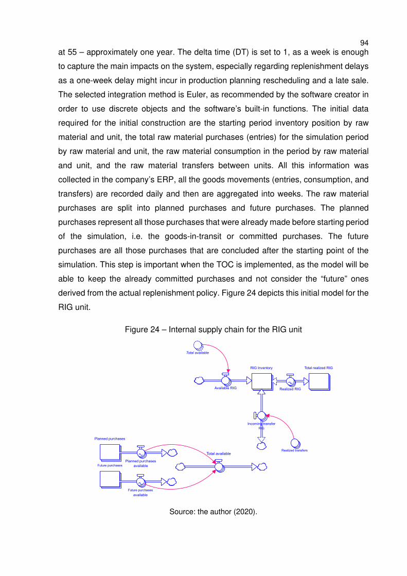
94 at 55 – approximately one year. The delta time (DT) is set to 1, as a week is enough
to capture the main impacts on the system, especially regarding replenishment delays
as a one-week delay might incur in production planning rescheduling and a late sale.
The selected integration method is Euler, as recommended by the software creator in
order to use discrete objects and the software’s built-in functions. The initial data
required for the initial construction are the starting period inventory position by raw
material and unit, the total raw material purchases (entries) for the simulation period
by raw material and unit, the raw material consumption in the period by raw material
and unit, and the raw material transfers between units. All this information was
collected in the company’s ERP, all the goods movements (entries, consumption, and
transfers) are recorded daily and then are aggregated into weeks. The raw material
purchases are split into planned purchases and future purchases. The planned
purchases represent all those purchases that were already made before starting period
of the simulation, i.e. the goods-in-transit or committed purchases. The future
purchases are all those purchases that are concluded after the starting point of the
simulation. This step is important when the TOC is implemented, as the model will be
able to keep the already committed purchases and not consider the “future” ones
derived from the actual replenishment policy. Figure 24 depicts this initial model for the
RIG unit.
Figure 24 – Internal supply chain for the RIG unit
Source: the author (2020).
Total realized RIGRIG Inventory
Future purchases
Planned purchases
Incoming transfer
RIG
Realized RIGAvailable RIG
Realized transfersTotal available
Future purchases
available
Planned purchases
available
Total available
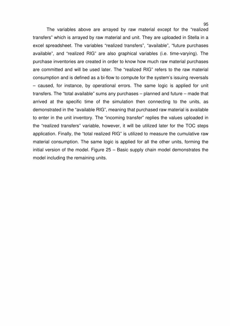
95 The variables above are arrayed by raw material except for the “realized
transfers” which is arrayed by raw material and unit. They are uploaded in Stella in a
excel spreadsheet. The variables “realized transfers”, “available”, “future purchases
available”, and “realized RIG” are also graphical variables (i.e. time-varying). The
purchase inventories are created in order to know how much raw material purchases
are committed and will be used later. The “realized RIG” refers to the raw material
consumption and is defined as a bi-flow to compute for the system’s issuing reversals
– caused, for instance, by operational errors. The same logic is applied for unit
transfers. The “total available” sums any purchases – planned and future – made that
arrived at the specific time of the simulation then connecting to the units, as
demonstrated in the “available RIG”, meaning that purchased raw material is available
to enter in the unit inventory. The “incoming transfer” replies the values uploaded in
the “realized transfers” variable, however, it will be utilized later for the TOC steps
application. Finally, the “total realized RIG” is utilized to measure the cumulative raw
material consumption. The same logic is applied for all the other units, forming the
initial version of the model. Figure 25 – Basic supply chain model demonstrates the
model including the remaining units.
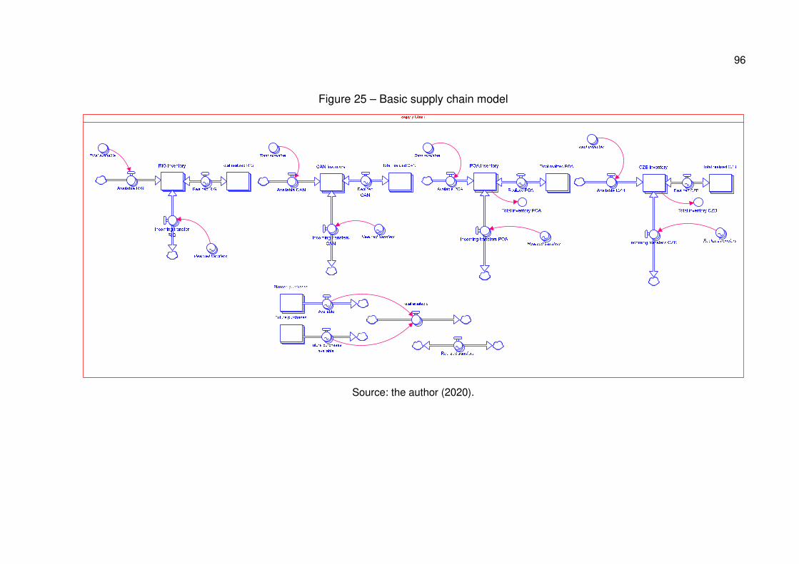
96
Figure 25 – Basic supply chain model
Source: the author (2020).
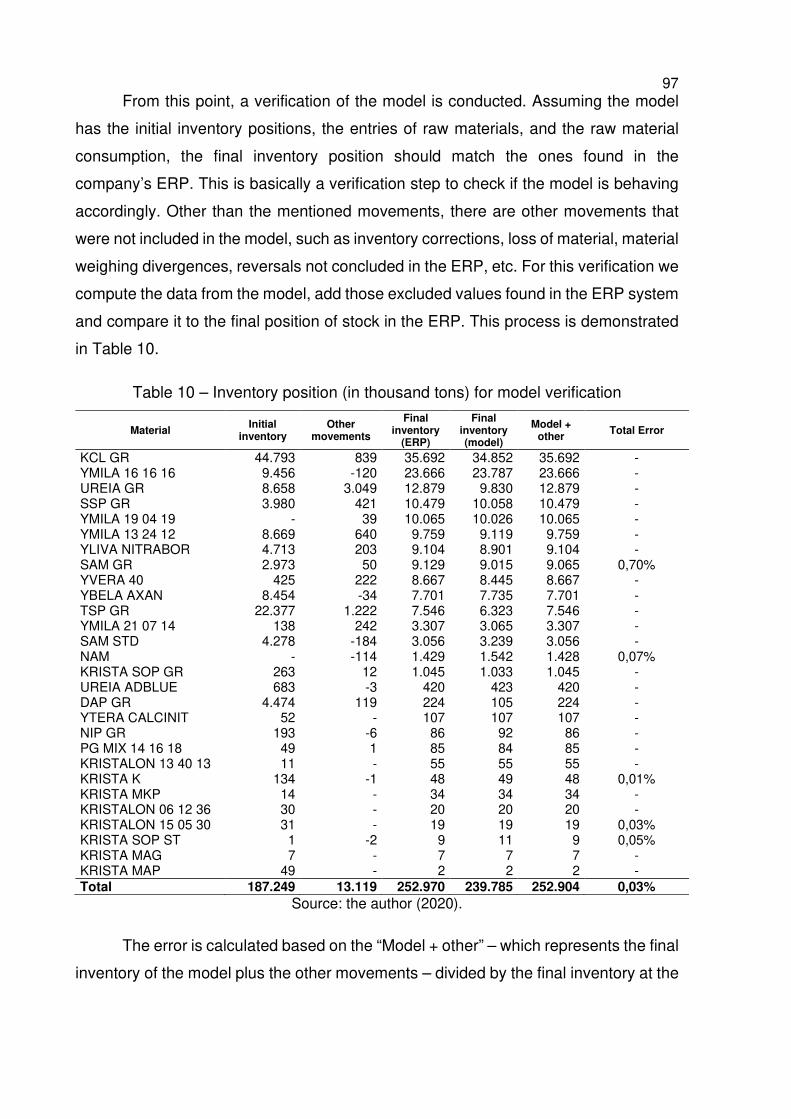
97 From this point, a verification of the model is conducted. Assuming the model
has the initial inventory positions, the entries of raw materials, and the raw material
consumption, the final inventory position should match the ones found in the
company’s ERP. This is basically a verification step to check if the model is behaving
accordingly. Other than the mentioned movements, there are other movements that
were not included in the model, such as inventory corrections, loss of material, material
weighing divergences, reversals not concluded in the ERP, etc. For this verification we
compute the data from the model, add those excluded values found in the ERP system
and compare it to the final position of stock in the ERP. This process is demonstrated
in Table 10.
Table 10 – Inventory position (in thousand tons) for model verification
Material Initial
inventory Other
movements
Final inventory
(ERP)
Final inventory (model)
Model + other
Total Error
KCL GR 44.793 839 35.692 34.852 35.692 - YMILA 16 16 16 9.456 -120 23.666 23.787 23.666 - UREIA GR 8.658 3.049 12.879 9.830 12.879 - SSP GR 3.980 421 10.479 10.058 10.479 - YMILA 19 04 19 - 39 10.065 10.026 10.065 - YMILA 13 24 12 8.669 640 9.759 9.119 9.759 - YLIVA NITRABOR 4.713 203 9.104 8.901 9.104 - SAM GR 2.973 50 9.129 9.015 9.065 0,70% YVERA 40 425 222 8.667 8.445 8.667 - YBELA AXAN 8.454 -34 7.701 7.735 7.701 - TSP GR 22.377 1.222 7.546 6.323 7.546 - YMILA 21 07 14 138 242 3.307 3.065 3.307 - SAM STD 4.278 -184 3.056 3.239 3.056 - NAM - -114 1.429 1.542 1.428 0,07% KRISTA SOP GR 263 12 1.045 1.033 1.045 - UREIA ADBLUE 683 -3 420 423 420 - DAP GR 4.474 119 224 105 224 - YTERA CALCINIT 52 - 107 107 107 - NIP GR 193 -6 86 92 86 - PG MIX 14 16 18 49 1 85 84 85 - KRISTALON 13 40 13 11 - 55 55 55 - KRISTA K 134 -1 48 49 48 0,01% KRISTA MKP 14 - 34 34 34 - KRISTALON 06 12 36 30 - 20 20 20 - KRISTALON 15 05 30 31 - 19 19 19 0,03% KRISTA SOP ST 1 -2 9 11 9 0,05% KRISTA MAG 7 - 7 7 7 - KRISTA MAP 49 - 2 2 2 - Total 187.249 13.119 252.970 239.785 252.904 0,03%
Source: the author (2020).
The error is calculated based on the “Model + other” – which represents the final
inventory of the model plus the other movements – divided by the final inventory at the
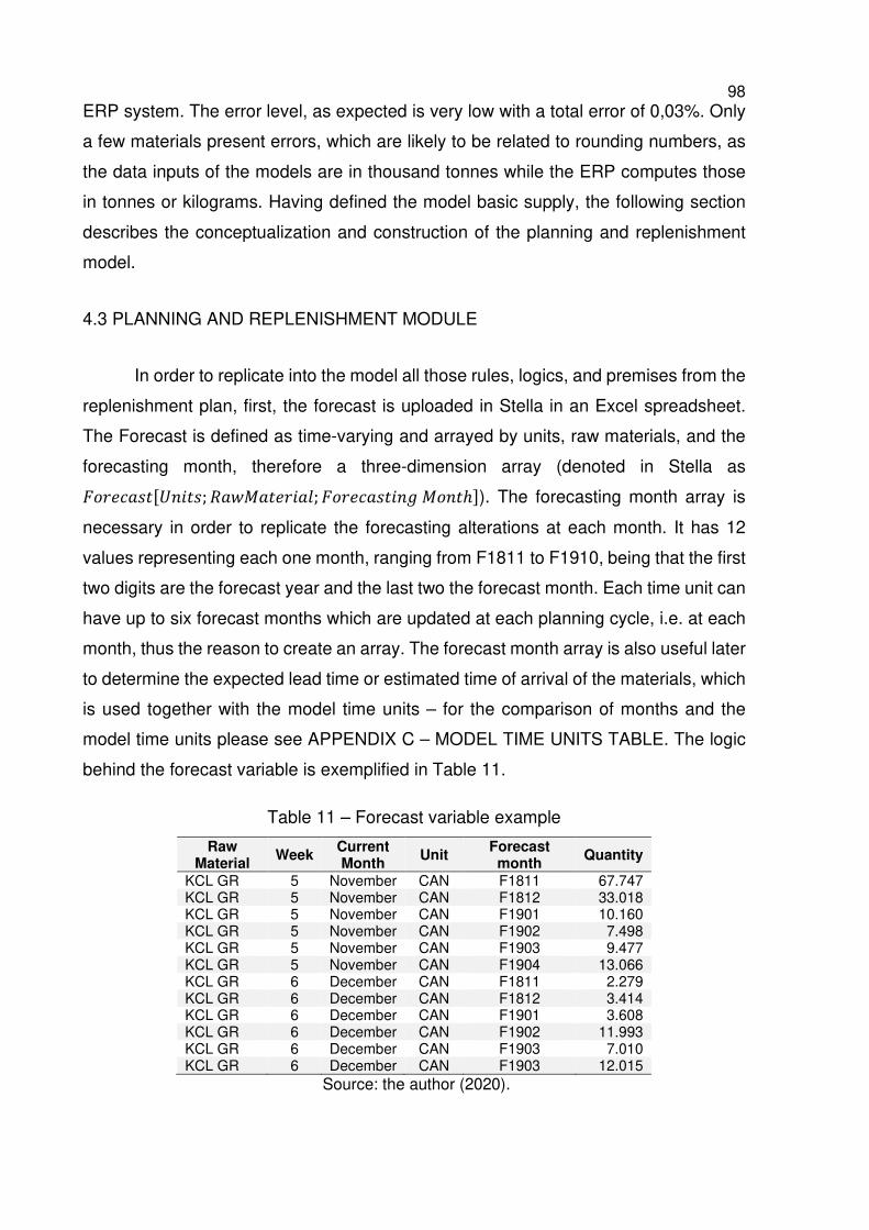
98 ERP system. The error level, as expected is very low with a total error of 0,03%. Only
a few materials present errors, which are likely to be related to rounding numbers, as
the data inputs of the models are in thousand tonnes while the ERP computes those
in tonnes or kilograms. Having defined the model basic supply, the following section
describes the conceptualization and construction of the planning and replenishment
model.
4.3 PLANNING AND REPLENISHMENT MODULE
In order to replicate into the model all those rules, logics, and premises from the
replenishment plan, first, the forecast is uploaded in Stella in an Excel spreadsheet.
The Forecast is defined as time-varying and arrayed by units, raw materials, and the
forecasting month, therefore a three-dimension array (denoted in Stella as
��������78����; ��- �������; ����������' ���ℎ9). The forecasting month array is
necessary in order to replicate the forecasting alterations at each month. It has 12
values representing each one month, ranging from F1811 to F1910, being that the first
two digits are the forecast year and the last two the forecast month. Each time unit can
have up to six forecast months which are updated at each planning cycle, i.e. at each
month, thus the reason to create an array. The forecast month array is also useful later
to determine the expected lead time or estimated time of arrival of the materials, which
is used together with the model time units – for the comparison of months and the
model time units please see APPENDIX C – MODEL TIME UNITS TABLE. The logic
behind the forecast variable is exemplified in Table 11.
Table 11 – Forecast variable example
Raw Material
Week Current Month
Unit Forecast month
Quantity
KCL GR 5 November CAN F1811 67.747 KCL GR 5 November CAN F1812 33.018 KCL GR 5 November CAN F1901 10.160 KCL GR 5 November CAN F1902 7.498 KCL GR 5 November CAN F1903 9.477 KCL GR 5 November CAN F1904 13.066 KCL GR 6 December CAN F1811 2.279 KCL GR 6 December CAN F1812 3.414 KCL GR 6 December CAN F1901 3.608 KCL GR 6 December CAN F1902 11.993 KCL GR 6 December CAN F1903 7.010 KCL GR 6 December CAN F1903 12.015
Source: the author (2020).
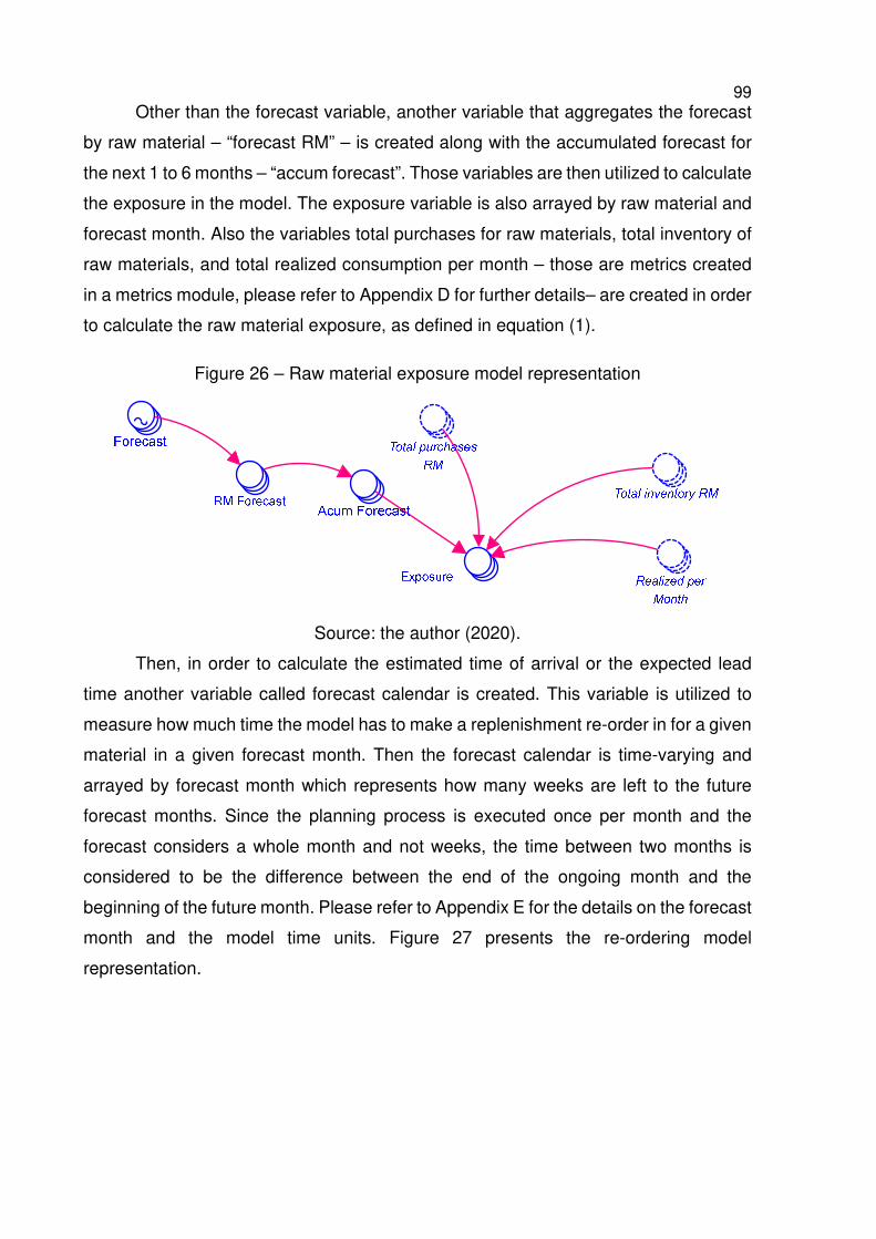
99 Other than the forecast variable, another variable that aggregates the forecast
by raw material – “forecast RM” – is created along with the accumulated forecast for
the next 1 to 6 months – “accum forecast”. Those variables are then utilized to calculate
the exposure in the model. The exposure variable is also arrayed by raw material and
forecast month. Also the variables total purchases for raw materials, total inventory of
raw materials, and total realized consumption per month – those are metrics created
in a metrics module, please refer to Appendix D for further details– are created in order
to calculate the raw material exposure, as defined in equation (1).
Figure 26 – Raw material exposure model representation
Source: the author (2020).
Then, in order to calculate the estimated time of arrival or the expected lead
time another variable called forecast calendar is created. This variable is utilized to
measure how much time the model has to make a replenishment re-order in for a given
material in a given forecast month. Then the forecast calendar is time-varying and
arrayed by forecast month which represents how many weeks are left to the future
forecast months. Since the planning process is executed once per month and the
forecast considers a whole month and not weeks, the time between two months is
considered to be the difference between the end of the ongoing month and the
beginning of the future month. Please refer to Appendix E for the details on the forecast
month and the model time units. Figure 27 presents the re-ordering model
representation.
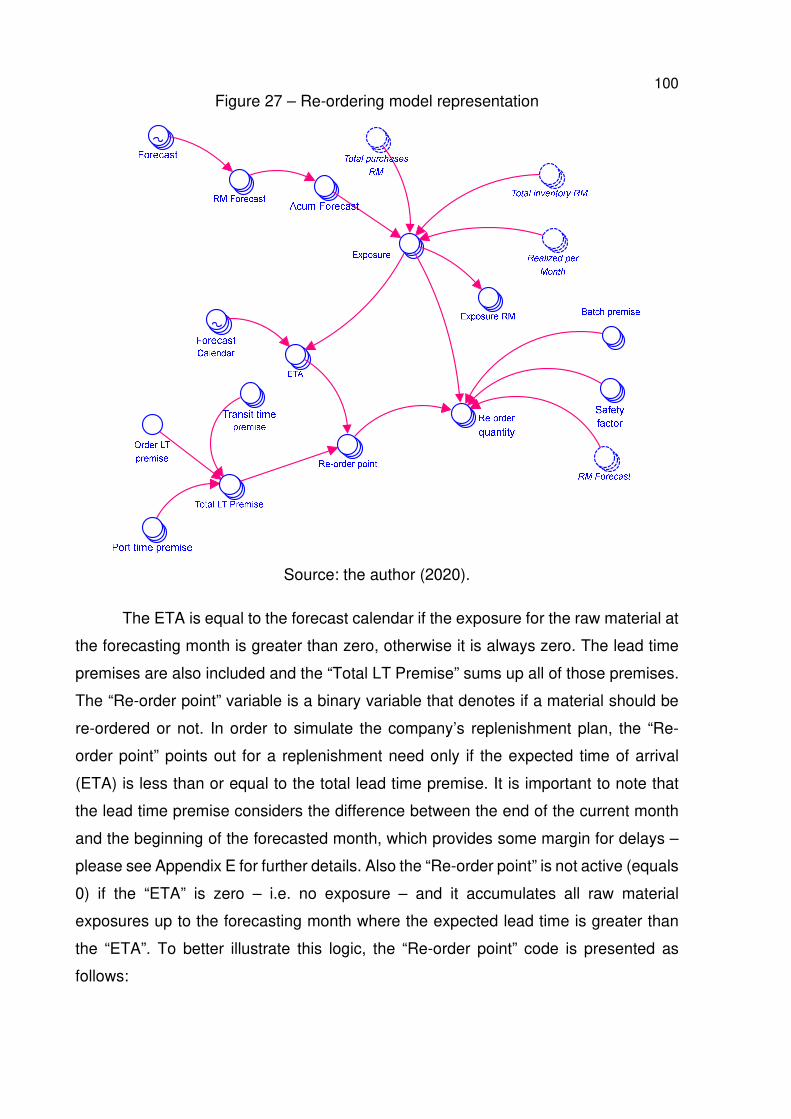
100 Figure 27 – Re-ordering model representation
Source: the author (2020).
The ETA is equal to the forecast calendar if the exposure for the raw material at
the forecasting month is greater than zero, otherwise it is always zero. The lead time
premises are also included and the “Total LT Premise” sums up all of those premises.
The “Re-order point” variable is a binary variable that denotes if a material should be
re-ordered or not. In order to simulate the company’s replenishment plan, the “Re-
order point” points out for a replenishment need only if the expected time of arrival
(ETA) is less than or equal to the total lead time premise. It is important to note that
the lead time premise considers the difference between the end of the current month
and the beginning of the forecasted month, which provides some margin for delays –
please see Appendix E for further details. Also the “Re-order point” is not active (equals
0) if the “ETA” is zero – i.e. no exposure – and it accumulates all raw material
exposures up to the forecasting month where the expected lead time is greater than
the “ETA”. To better illustrate this logic, the “Re-order point” code is presented as
follows:
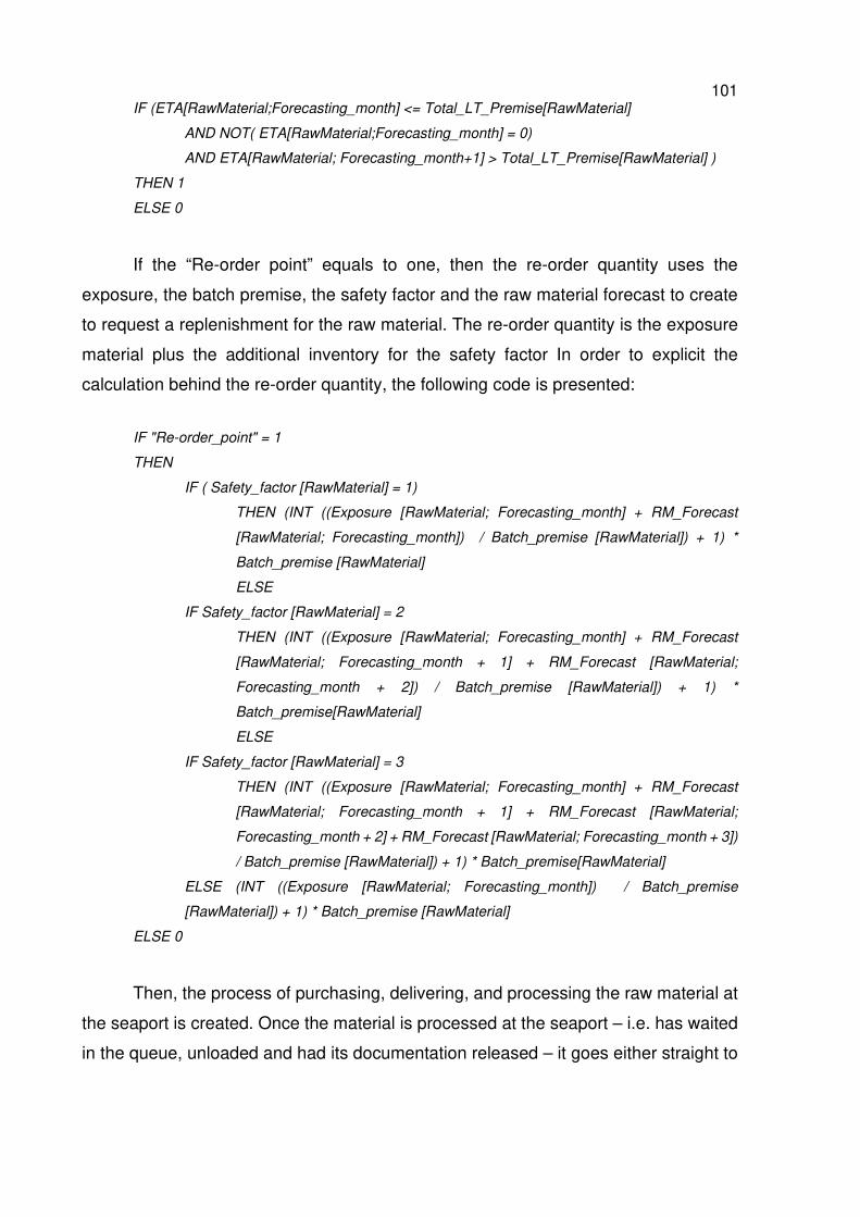
101 IF (ETA[RawMaterial;Forecasting_month] <= Total_LT_Premise[RawMaterial]
AND NOT( ETA[RawMaterial;Forecasting_month] = 0)
AND ETA[RawMaterial; Forecasting_month+1] > Total_LT_Premise[RawMaterial] )
THEN 1
ELSE 0
If the “Re-order point” equals to one, then the re-order quantity uses the
exposure, the batch premise, the safety factor and the raw material forecast to create
to request a replenishment for the raw material. The re-order quantity is the exposure
material plus the additional inventory for the safety factor In order to explicit the
calculation behind the re-order quantity, the following code is presented:
IF "Re-order_point" = 1
THEN
IF ( Safety_factor [RawMaterial] = 1)
THEN (INT ((Exposure [RawMaterial; Forecasting_month] + RM_Forecast
[RawMaterial; Forecasting_month]) / Batch_premise [RawMaterial]) + 1) *
Batch_premise [RawMaterial]
ELSE
IF Safety_factor [RawMaterial] = 2
THEN (INT ((Exposure [RawMaterial; Forecasting_month] + RM_Forecast
[RawMaterial; Forecasting_month + 1] + RM_Forecast [RawMaterial;
Forecasting_month + 2]) / Batch_premise [RawMaterial]) + 1) *
Batch_premise[RawMaterial]
ELSE
IF Safety_factor [RawMaterial] = 3
THEN (INT ((Exposure [RawMaterial; Forecasting_month] + RM_Forecast
[RawMaterial; Forecasting_month + 1] + RM_Forecast [RawMaterial;
Forecasting_month + 2] + RM_Forecast [RawMaterial; Forecasting_month + 3])
/ Batch_premise [RawMaterial]) + 1) * Batch_premise[RawMaterial]
ELSE (INT ((Exposure [RawMaterial; Forecasting_month]) / Batch_premise
[RawMaterial]) + 1) * Batch_premise [RawMaterial]
ELSE 0
Then, the process of purchasing, delivering, and processing the raw material at
the seaport is created. Once the material is processed at the seaport – i.e. has waited
in the queue, unloaded and had its documentation released – it goes either straight to
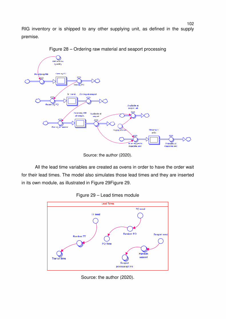
102 RIG inventory or is shipped to any other supplying unit, as defined in the supply
premise.
Figure 28 – Ordering raw material and seaport processing
Source: the author (2020).
All the lead time variables are created as ovens in order to have the order wait
for their lead times. The model also simulates those lead times and they are inserted
in its own module, as illustrated in Figure 29Figure 29.
Figure 29 – Lead times module
Source: the author (2020).
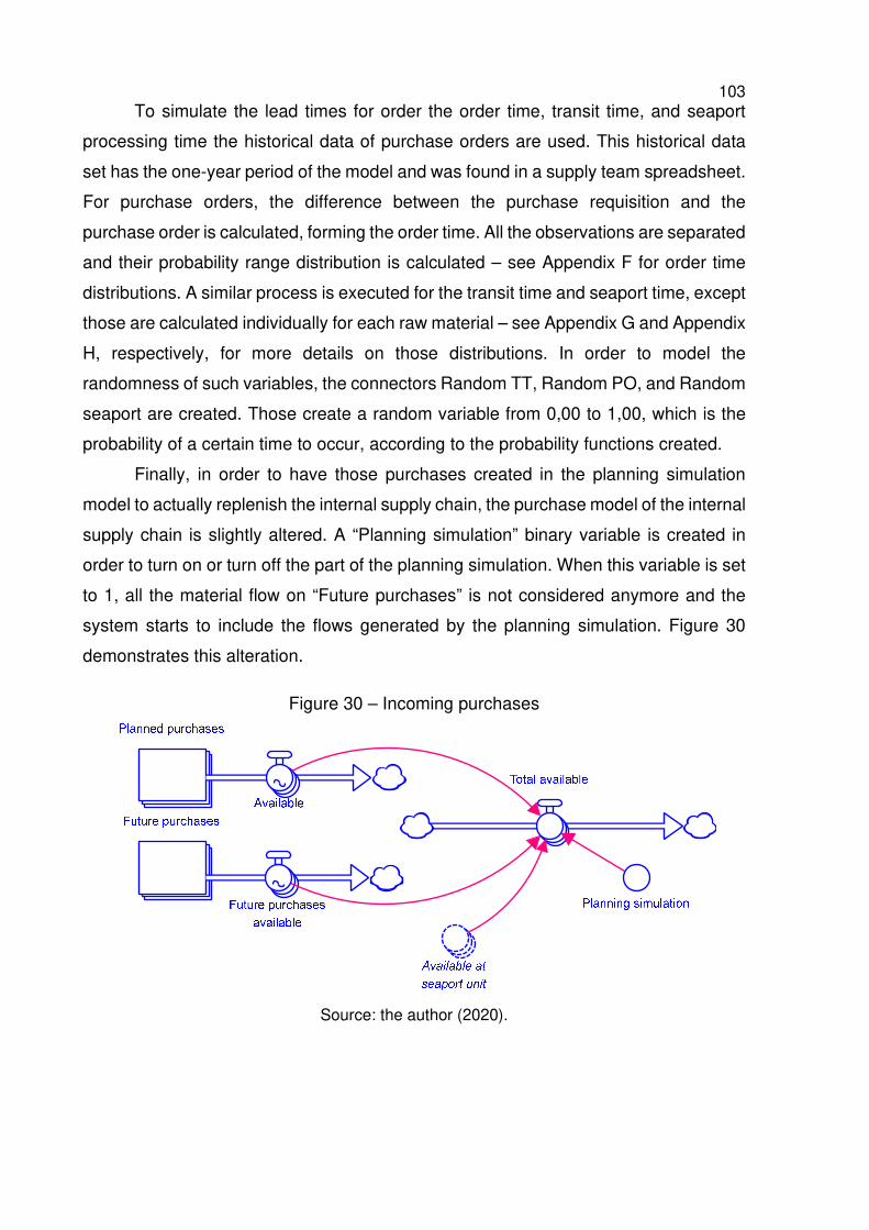
103 To simulate the lead times for order the order time, transit time, and seaport
processing time the historical data of purchase orders are used. This historical data
set has the one-year period of the model and was found in a supply team spreadsheet.
For purchase orders, the difference between the purchase requisition and the
purchase order is calculated, forming the order time. All the observations are separated
and their probability range distribution is calculated – see Appendix F for order time
distributions. A similar process is executed for the transit time and seaport time, except
those are calculated individually for each raw material – see Appendix G and Appendix
H, respectively, for more details on those distributions. In order to model the
randomness of such variables, the connectors Random TT, Random PO, and Random
seaport are created. Those create a random variable from 0,00 to 1,00, which is the
probability of a certain time to occur, according to the probability functions created.
Finally, in order to have those purchases created in the planning simulation
model to actually replenish the internal supply chain, the purchase model of the internal
supply chain is slightly altered. A “Planning simulation” binary variable is created in
order to turn on or turn off the part of the planning simulation. When this variable is set
to 1, all the material flow on “Future purchases” is not considered anymore and the
system starts to include the flows generated by the planning simulation. Figure 30
demonstrates this alteration.
Figure 30 – Incoming purchases
Source: the author (2020).
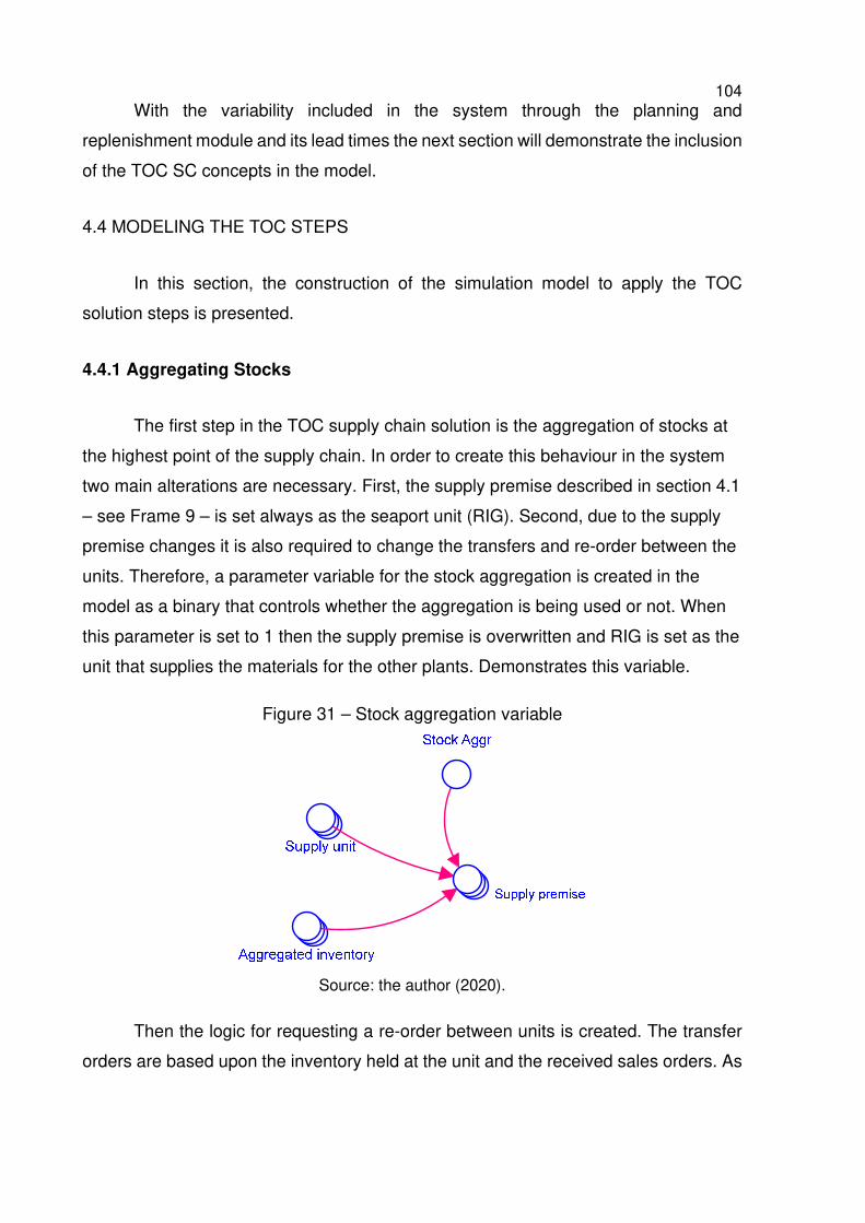
104 With the variability included in the system through the planning and
replenishment module and its lead times the next section will demonstrate the inclusion
of the TOC SC concepts in the model.
4.4 MODELING THE TOC STEPS
In this section, the construction of the simulation model to apply the TOC
solution steps is presented.
4.4.1 Aggregating Stocks
The first step in the TOC supply chain solution is the aggregation of stocks at
the highest point of the supply chain. In order to create this behaviour in the system
two main alterations are necessary. First, the supply premise described in section 4.1
– see Frame 9 – is set always as the seaport unit (RIG). Second, due to the supply
premise changes it is also required to change the transfers and re-order between the
units. Therefore, a parameter variable for the stock aggregation is created in the
model as a binary that controls whether the aggregation is being used or not. When
this parameter is set to 1 then the supply premise is overwritten and RIG is set as the
unit that supplies the materials for the other plants. Demonstrates this variable.
Figure 31 – Stock aggregation variable
Source: the author (2020).
Then the logic for requesting a re-order between units is created. The transfer
orders are based upon the inventory held at the unit and the received sales orders. As
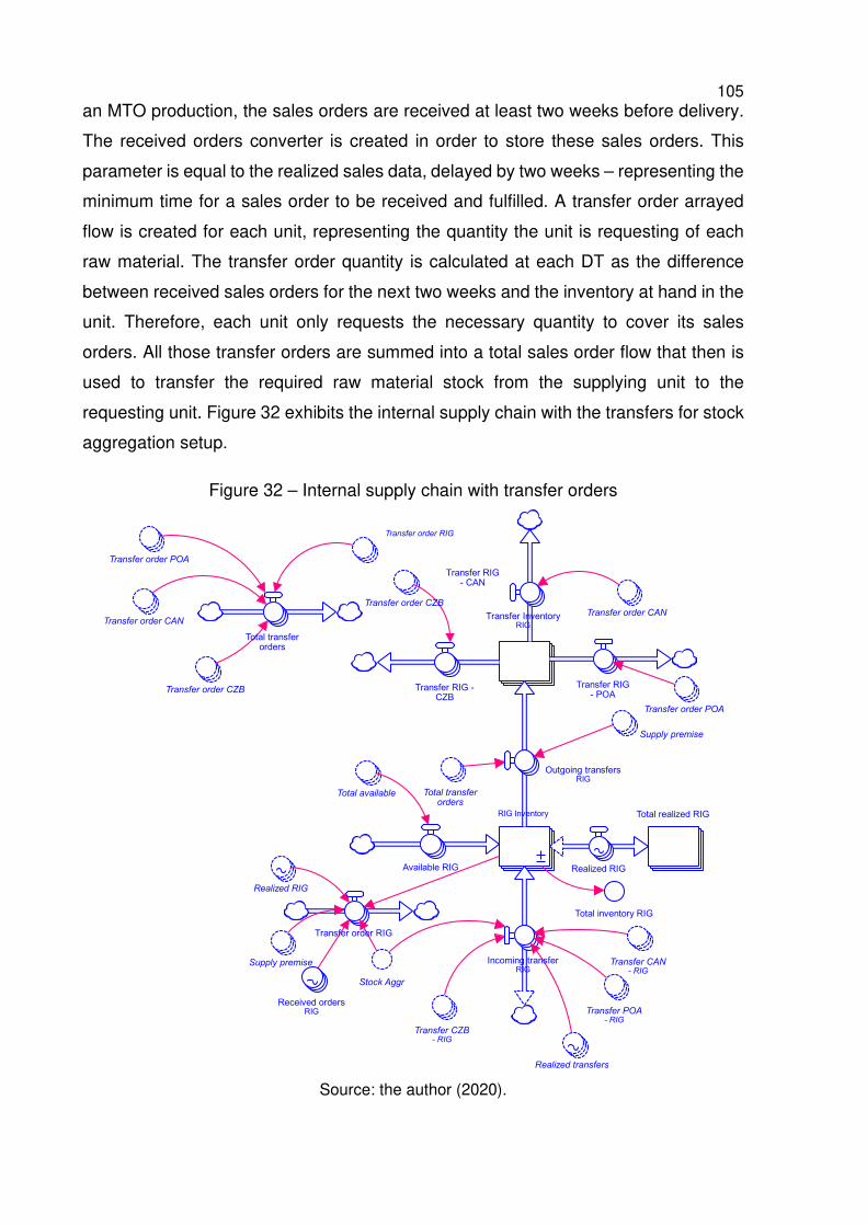
105 an MTO production, the sales orders are received at least two weeks before delivery.
The received orders converter is created in order to store these sales orders. This
parameter is equal to the realized sales data, delayed by two weeks – representing the
minimum time for a sales order to be received and fulfilled. A transfer order arrayed
flow is created for each unit, representing the quantity the unit is requesting of each
raw material. The transfer order quantity is calculated at each DT as the difference
between received sales orders for the next two weeks and the inventory at hand in the
unit. Therefore, each unit only requests the necessary quantity to cover its sales
orders. All those transfer orders are summed into a total sales order flow that then is
used to transfer the required raw material stock from the supplying unit to the
requesting unit. Figure 32 exhibits the internal supply chain with the transfers for stock
aggregation setup.
Figure 32 – Internal supply chain with transfer orders
Source: the author (2020).
Transfer InventoryRIG
Total realized RIGRIG Inventory
Incoming transferRIG
Total transferorders
Received ordersRIG
Total inventory RIG
Supply premise
Realized transfers
Stock Aggr
Supply premise
Realized RIG
Transfer order CAN
Transfer CZB- RIG
Transfer order RIG
Total transferorders
Transfer POA- RIG
Transfer CAN- RIG
Total available
Transfer order POA
Transfer order CZB
Transfer order POA
Transfer order CANTransfer order CZB
Transfer RIG- POA
Transfer RIG -CZB
Transfer order RIG
Transfer RIG- CAN
Available RIG
Outgoing transfersRIG
Realized RIG
106 The outgoing transfer flow is created to simulate an outgoing material from the
supplying unit inventory to the transfer inventory. From the transfer inventory then the
raw materials are “send” to the requesting unit – represented the transfer flows for each
unit – and available in the incoming transfer flow of the respective unit. In that sense,
the transfer orders are available one week after the request, which is the real lead time
for such transfers. The next section covers the modeling of buffer sizes and the TOC
RLT and described.
4.4.2 Determining Buffer Sizes Based on Demand, Supply, and The
Replenishment Lead
To create the remaining steps of the TOC another module needs to be created
and some alterations are to be made in the planning module. A few binary parameters
are created in order to control the TOC steps application. For this step specifically the
parameters created are the TOC buffer and the TOC RLT. The TOC size is defined as
proposed by Youngman (2009):
:�//�� ���� = ������ �� − ����� ���� ∗ �+���'� �����������
+ ������� �/ ��/��, (3)
The measure of safety is usually defined as 50%. The maximum time is
calculated based on the historical supply data, while the weekly average consumption
of the raw materials. Both variables are uploaded in the model by raw material in an
excel spreadsheet. Then to simulate the replenishment lead time reduction proposed
by the TOC, when the TOC RLT parameter is set to 1 there is no time from the
identification of replenishment and the creation of the re-order; therefore, the RLT is 0
and the re-order is set directly to in transit, meaning that the supplier is already
processing that order. It is important to note that, in this step, the model still uses the
forecast to know when to issue a re-order. It only uses the buffer size in order to
determine the re-order quantity. Having described the buffer sizing, the management
of inventory using buffer penetration is presented next.
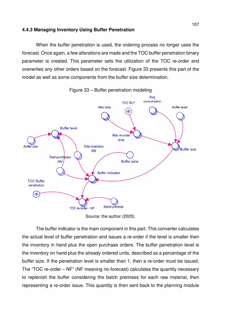
107 4.4.3 Managing Inventory Using Buffer Penetration
When the buffer penetration is used, the ordering process no longer uses the
forecast. Once again, a few alterations are made and the TOC buffer penetration binary
parameter is created. This parameter sets the utilization of the TOC re-order and
overwrites any other orders based on the forecast. Figure 33 presents this part of the
model as well as some components from the buffer size determination.
Figure 33 – Buffer penetration modeling
Source: the author (2020).
The buffer indicator is the main component in this part. This converter calculates
the actual level of buffer penetration and issues a re-order if the level is smaller then
the inventory in hand plus the open purchase orders. The buffer penetration level is
the inventory on hand plus the already ordered units, described as a percentage of the
buffer size. If the penetration level is smaller than 1, then a re-order must be issued.
The “TOC re-order – NF” (NF meaning no-forecast) calculates the quantity necessary
to replenish the buffer considering the batch premises for each raw material, then
representing a re-order issue. This quantity is then sent back to the planning module
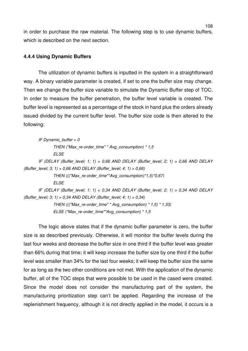
108 in order to purchase the raw material. The following step is to use dynamic buffers,
which is described on the next section.
4.4.4 Using Dynamic Buffers
The utilization of dynamic buffers is inputted in the system in a straightforward
way. A binary variable parameter is created, if set to one the buffer size may change.
Then we change the buffer size variable to simulate the Dynamic Buffer step of TOC.
In order to measure the buffer penetration, the buffer level variable is created. The
buffer level is represented as a percentage of the stock in hand plus the orders already
issued divided by the current buffer level. The buffer size code is then altered to the
following:
IF Dynamic_buffer = 0
THEN ("Max_re-order_time" * Avg_consumption) * 1,5
ELSE
IF (DELAY (Buffer_level; 1; 1) > 0,66 AND DELAY (Buffer_level; 2; 1) > 0,66 AND DELAY
(Buffer_level; 3; 1) > 0,66 AND DELAY (Buffer_level; 4; 1) > 0,66)
THEN ((("Max_re-order_time"*Avg_consumption)*1,5)*0,67)
ELSE
IF (DELAY (Buffer_level; 1; 1) < 0,34 AND DELAY (Buffer_level; 2; 1) > 0,34 AND DELAY
(Buffer_level; 3; 1) > 0,34 AND DELAY (Buffer_level; 4; 1) > 0,34)
THEN ((("Max_re-order_time" * Avg_consumption) * 1,5) * 1,33)
ELSE ("Max_re-order_time"*Avg_consumption) * 1,5
The logic above states that if the dynamic buffer parameter is zero, the buffer
size is as described previously. Otherwise, it will monitor the buffer levels during the
last four weeks and decrease the buffer size in one third if the buffer level was greater
than 66% during that time; it will keep increase the buffer size by one third if the buffer
level was smaller than 34% for the last four weeks; it will keep the buffer size the same
for as long as the two other conditions are not met. With the application of the dynamic
buffer, all of the TOC steps that were possible to be used in the cased were created.
Since the model does not consider the manufacturing part of the system, the
manufacturing prioritization step can’t be applied. Regarding the increase of the
replenishment frequency, although it is not directly applied in the model, it occurs is a
109 consequence of the aggregation of stocks and the utilization of the TOC buffers. The
replenishment frequency will be covered in detail in the data analysis section. In the
next section, a hybrid solution considering the case specificities and the TOC solution
is described and modeled.
4.4.5 Creating a Hybrid Solution Utilizing Buffers and Forecast
A hybrid model that uses the TOC buffer management and some information
from the forecast is also proposed. This model is created to measure if it is possible to
use the forecast information in conjunction with the TOC solution to achieve better
results than the proposed steps and to deal with seasonality from the case.
Schragenheim (2010) affirms that TOC’s DBM does not handle well seasonality in
demand and even proposes a few techniques to improve the method. This method is
rather simplistic tough, consisting of disabling the dynamic buffer and stocking up prior
to high seasons and the opposite to deal with sudden decreases of demand. In order
to foresee seasonality patterns then, the forecast is still used. The current model
creates a hybrid solution utilizing TOC solution steps and drawing information from the
forecast.
The main change regards the buffer size and the re-ordering point. To do so a
“buffer size FB” (forecast-based) is created. This buffer size is set according to the
accumulated forecast of the forecast month and only replenished if the estimated time
of arrival is smaller than or equal to the remaining time to that specific month. This re-
order point is quite similar to the one that is utilized in the model currently. The buffer
size is defined as:
:�//�� ���� �: = �∑ ���������� ����������� ���� � −
�������� ���ℎ "����#$ � ∗ 1,5 (4)
Then if the buffer size is smaller than the inventory in hand and the raw material
already ordered must be issued to replenish the buffer. In the model, the TOC re-order
based on the forecast is calculated based on the quantity necessary to replenish the
buffer plus the estimated time of arrival of the material for that future month. This
follows the same logic as in the planning module and is with the TOC as well. Along
110 with the other TOC steps described, this part composes the TOC planning module, as
shown in Figure 34.
Figure 34 – TOC planning module
Source: the author (2020).
The presentation of the TOC planning module concludes all the modeling logic
created. An additional module, however, is necessary in order to have the TOC
performance measure, as well as many other indicators of inventory and consumption.
Then, the performance measures module is presented next.
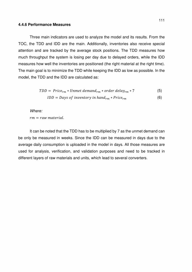
111 4.4.6 Performance Measures
Three main indicators are used to analyze the model and its results. From the
TOC, the TDD and IDD are the main. Additionally, inventories also receive special
attention and are tracked by the average stock positions. The TDD measures how
much throughput the system is losing per day due to delayed orders, while the IDD
measures how well the inventories are positioned (the right material at the right time).
The main goal is to minimize the TDD while keeping the IDD as low as possible. In the
model, the TDD and the IDD are calculated as:
1?? = (���� ∗ 8���� ������ ∗ ����� ����, ∗ 7 (5)
*?? = ?�,� �/ ��+�����, �� ℎ��� ∗ (���� (6)
Where:
�� = ��- ��������.
It can be noted that the TDD has to be multiplied by 7 as the unmet demand can
be only be measured in weeks. Since the IDD can be measured in days due to the
average daily consumption is uploaded in the model in days. All those measures are
used for analysis, verification, and validation purposes and need to be tracked in
different layers of raw materials and units, which lead to several converters.
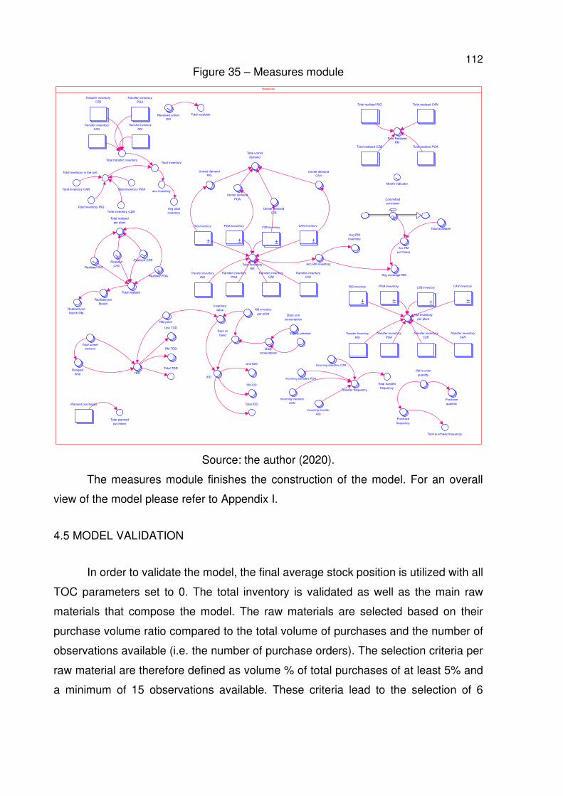
112 Figure 35 – Measures module
Source: the author (2020).
The measures module finishes the construction of the model. For an overall
view of the model please refer to Appendix I.
4.5 MODEL VALIDATION
In order to validate the model, the final average stock position is utilized with all
TOC parameters set to 0. The total inventory is validated as well as the main raw
materials that compose the model. The raw materials are selected based on their
purchase volume ratio compared to the total volume of purchases and the number of
observations available (i.e. the number of purchase orders). The selection criteria per
raw material are therefore defined as volume % of total purchases of at least 5% and
a minimum of 15 observations available. These criteria lead to the selection of 6
Measures
Transfer inventory
CZB
Transfer inventory
CAN
Transfer inventory
POA
Transfer inventory
CZB
POA Inventory CAN Inventory
Transfer inventory
CZB
Total realized CAN
Transfer inventory
POA
CAN InventoryPOA Inventory
Transfer inventory
POA
Total realized RIG
Transfer Inventory
RIG
CZB InventoryRIG Inventory
Planned purchases
Transfer Inventory
RIG
Transfer inventory
CAN
Transfer inventory
CAN
Total realized POA
Transfer Inventory
RIG
Total realized CZB
CZB InventoryRIG Inventory
Total recebido
Total realized
Unmet demand
POA
Unmet demand
RIG
Unmet demand
CZB
Unmet demand
CANTotal inventory in the unit
Total InventoryTotal transfer Inventory
Total inventory
RM
Total unmet
demand
Total Realized
RM
Realized per
Month
Month Indicator
Realized per
Month RM
Incoming transfer
RIG
Incoming transfers
CAN
Incoming transfers POA
Incoming transfers CZB
Total inventory CZB
Acc RM inventory
Total inventory POAacc inventory
Avg total
inventory
Total inventory RIG
Avg RM
inventory
Total available
Realized
CAN
Avg coverage RM
Acc RM
purchases
Realized CZB
Supply premise
Total inventory CAN
Realized RIG
Realized POA
RM price
IDD
TDDDelayed
time
RM TDD
Unit TDD
Total TDD
RM Inventory
per plant
Total realized
per plant
Inventory
value
Daily unit
consumption
Days on
hand
Received orders
RIG
RM IDD
Unit IDD
Total IDD
Daily
consumption
Purchase
frequency
Purchase
quantity
Total purchase frequency
Transfer frequency
Total transfer
frequency
Total planned
purchases
Total unmet
demand
RM Inventory
per plant
RM re-order
quantity
Committed
purchases
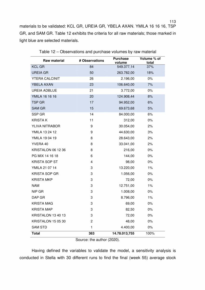
113 materials to be validated: KCL GR, UREIA GR, YBELA AXAN. YMILA 16 16 16, TSP
GR, and SAM GR. Table 12 exhibits the criteria for all raw materials; those marked in
light blue are selected materials.
Table 12 – Observations and purchase volumes by raw material
Raw material # Observations Purchase volume
Volume % of total
KCL GR 84 549.377,14 37%
UREIA GR 50 263.782,00 18%
YTERA CALCINIT 26 2.196,00 0%
YBELA AXAN 23 106.640,00 7%
UREIA ADBLUE 21 3.772,00 0%
YMILA 16 16 16 20 124.908,44 8%
TSP GR 17 94.952,00 6%
SAM GR 15 69.673,68 5%
SSP GR 14 84.000,00 6%
KRISTA K 11 312,00 0%
YLIVA NITRABOR 9 30.054,00 2%
YMILA 13 24 12 9 44.630,00 3%
YMILA 19 04 19 8 28.643,00 2%
YVERA 40 8 33.041,00 2%
KRISTALON 06 12 36 8 216,00 0%
PG MIX 14 16 18 6 144,00 0%
KRISTA SOP ST 4 98,00 0%
YMILA 21 07 14 3 13.220,00 1%
KRISTA SOP GR 3 1.056,00 0%
KRISTA MKP 3 72,00 0%
NAM 3 12.751,00 1%
NIP GR 3 1.008,00 0%
DAP GR 3 8.796,00 1%
KRISTA MAG 3 69,00 0%
KRISTA MAP 3 82,50 0%
KRISTALON 13 40 13 3 72,00 0%
KRISTALON 15 05 30 2 48,00 0%
SAM STD 1 4.400,00 0%
Total 363 14.78.013,755 100%
Source: the author (2020).
Having defined the variables to validate the model, a sensitivity analysis is
conducted in Stella with 30 different runs to find the final (week 55) average stock
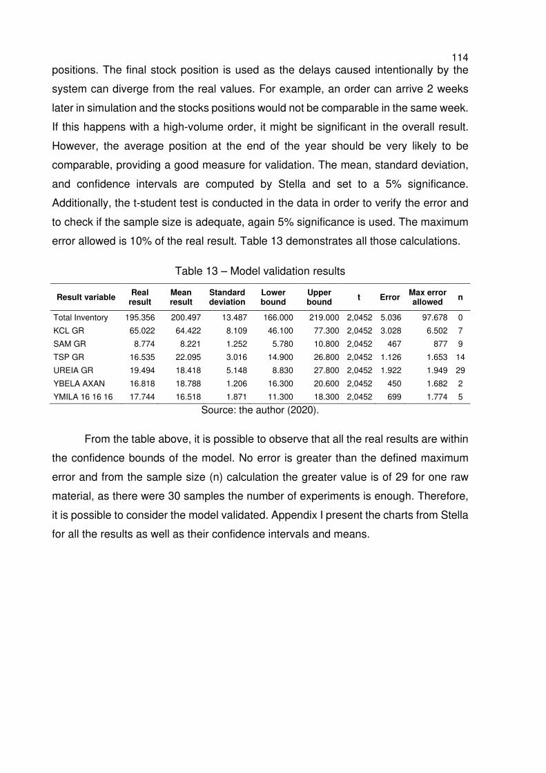
114 positions. The final stock position is used as the delays caused intentionally by the
system can diverge from the real values. For example, an order can arrive 2 weeks
later in simulation and the stocks positions would not be comparable in the same week.
If this happens with a high-volume order, it might be significant in the overall result.
However, the average position at the end of the year should be very likely to be
comparable, providing a good measure for validation. The mean, standard deviation,
and confidence intervals are computed by Stella and set to a 5% significance.
Additionally, the t-student test is conducted in the data in order to verify the error and
to check if the sample size is adequate, again 5% significance is used. The maximum
error allowed is 10% of the real result. Table 13 demonstrates all those calculations.
Table 13 – Model validation results
Result variable Real
result Mean result
Standard deviation
Lower bound
Upper bound
t Error Max error allowed
n
Total Inventory 195.356 200.497 13.487 166.000 219.000 2,0452 5.036 97.678 0
KCL GR 65.022 64.422 8.109 46.100 77.300 2,0452 3.028 6.502 7
SAM GR 8.774 8.221 1.252 5.780 10.800 2,0452 467 877 9
TSP GR 16.535 22.095 3.016 14.900 26.800 2,0452 1.126 1.653 14
UREIA GR 19.494 18.418 5.148 8.830 27.800 2,0452 1.922 1.949 29
YBELA AXAN 16.818 18.788 1.206 16.300 20.600 2,0452 450 1.682 2
YMILA 16 16 16 17.744 16.518 1.871 11.300 18.300 2,0452 699 1.774 5
Source: the author (2020).
From the table above, it is possible to observe that all the real results are within
the confidence bounds of the model. No error is greater than the defined maximum
error and from the sample size (n) calculation the greater value is of 29 for one raw
material, as there were 30 samples the number of experiments is enough. Therefore,
it is possible to consider the model validated. Appendix I present the charts from Stella
for all the results as well as their confidence intervals and means.
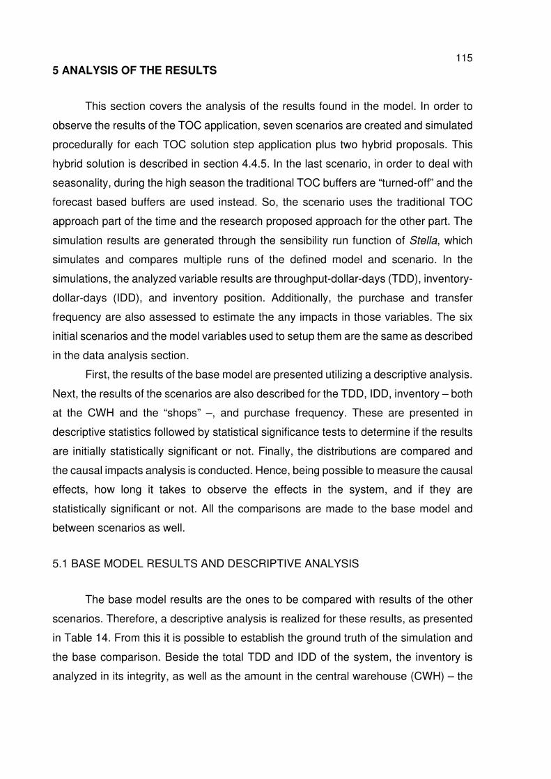
115 5 ANALYSIS OF THE RESULTS
This section covers the analysis of the results found in the model. In order to
observe the results of the TOC application, seven scenarios are created and simulated
procedurally for each TOC solution step application plus two hybrid proposals. This
hybrid solution is described in section 4.4.5. In the last scenario, in order to deal with
seasonality, during the high season the traditional TOC buffers are “turned-off” and the
forecast based buffers are used instead. So, the scenario uses the traditional TOC
approach part of the time and the research proposed approach for the other part. The
simulation results are generated through the sensibility run function of Stella, which
simulates and compares multiple runs of the defined model and scenario. In the
simulations, the analyzed variable results are throughput-dollar-days (TDD), inventory-
dollar-days (IDD), and inventory position. Additionally, the purchase and transfer
frequency are also assessed to estimate the any impacts in those variables. The six
initial scenarios and the model variables used to setup them are the same as described
in the data analysis section.
First, the results of the base model are presented utilizing a descriptive analysis.
Next, the results of the scenarios are also described for the TDD, IDD, inventory – both
at the CWH and the “shops” –, and purchase frequency. These are presented in
descriptive statistics followed by statistical significance tests to determine if the results
are initially statistically significant or not. Finally, the distributions are compared and
the causal impacts analysis is conducted. Hence, being possible to measure the causal
effects, how long it takes to observe the effects in the system, and if they are
statistically significant or not. All the comparisons are made to the base model and
between scenarios as well.
5.1 BASE MODEL RESULTS AND DESCRIPTIVE ANALYSIS
The base model results are the ones to be compared with results of the other
scenarios. Therefore, a descriptive analysis is realized for these results, as presented
in Table 14. From this it is possible to establish the ground truth of the simulation and
the base comparison. Beside the total TDD and IDD of the system, the inventory is
analyzed in its integrity, as well as the amount in the central warehouse (CWH) – the
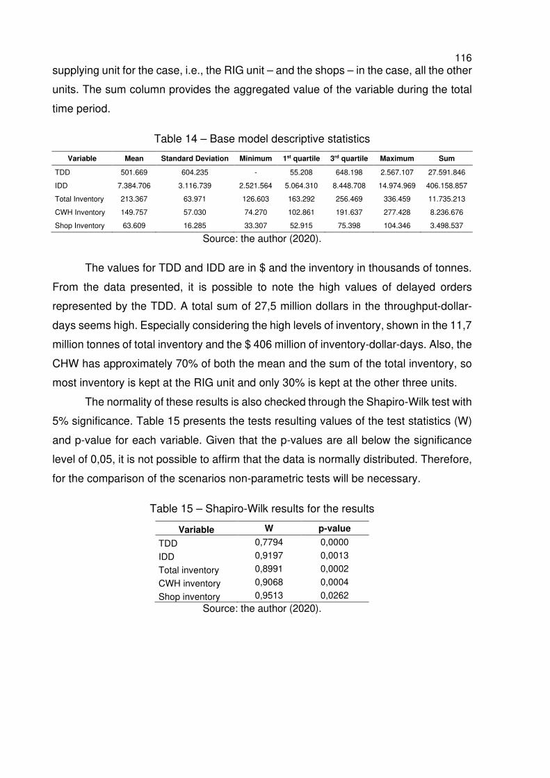
116 supplying unit for the case, i.e., the RIG unit – and the shops – in the case, all the other
units. The sum column provides the aggregated value of the variable during the total
time period.
Table 14 – Base model descriptive statistics
Variable Mean Standard Deviation Minimum 1st quartile 3rd quartile Maximum Sum
TDD 501.669 604.235 - 55.208 648.198 2.567.107 27.591.846
IDD 7.384.706 3.116.739 2.521.564 5.064.310 8.448.708 14.974.969 406.158.857
Total Inventory 213.367 63.971 126.603 163.292 256.469 336.459 11.735.213
CWH Inventory 149.757 57.030 74.270 102.861 191.637 277.428 8.236.676
Shop Inventory 63.609 16.285 33.307 52.915 75.398 104.346 3.498.537
Source: the author (2020).
The values for TDD and IDD are in $ and the inventory in thousands of tonnes.
From the data presented, it is possible to note the high values of delayed orders
represented by the TDD. A total sum of 27,5 million dollars in the throughput-dollar-
days seems high. Especially considering the high levels of inventory, shown in the 11,7
million tonnes of total inventory and the $ 406 million of inventory-dollar-days. Also, the
CHW has approximately 70% of both the mean and the sum of the total inventory, so
most inventory is kept at the RIG unit and only 30% is kept at the other three units.
The normality of these results is also checked through the Shapiro-Wilk test with
5% significance. Table 15 presents the tests resulting values of the test statistics (W)
and p-value for each variable. Given that the p-values are all below the significance
level of 0,05, it is not possible to affirm that the data is normally distributed. Therefore,
for the comparison of the scenarios non-parametric tests will be necessary.
Table 15 – Shapiro-Wilk results for the results
Variable W p-value
TDD 0,7794 0,0000
IDD 0,9197 0,0013
Total inventory 0,8991 0,0002
CWH inventory 0,9068 0,0004
Shop inventory 0,9513 0,0262 Source: the author (2020).
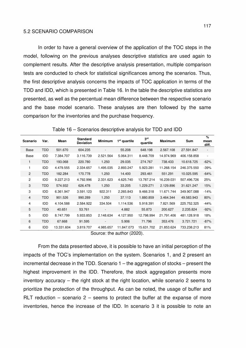
117 5.2 SCENARIO COMPARISON
In order to have a general overview of the application of the TOC steps in the
model, following on the previous analyses descriptive statistics are used again to
complement results. After the descriptive analysis presentation, multiple comparison
tests are conducted to check for statistical significances among the scenarios. Thus,
the first descriptive analysis concerns the impacts of TOC application in terms of the
TDD and IDD, which is presented in Table 16. In the table the descriptive statistics are
presented, as well as the percentual mean difference between the respective scenario
and the base model scenario. These analyses are then followed by the same
comparison for the inventories and the purchase frequency.
Table 16 – Scenarios descriptive analysis for TDD and IDD
Scenario Var. Mean Standard Deviation
Minimum 1st quartile 3rd
quartile Maximum Sum
% mean diff.
Base TDD 501.670 604.235 - 55.208 648.198 2.567.108 27.591.847 -
Base IDD 7.384.707 3.116.739 2.521.564 5.064.311 8.448.709 14.974.969 406.158.858 -
1 TDD 193.068 220.780 1.250 29.035 274.767 738.433 10.618.725 -62%
1 IDD 4.479.555 2.334.657 1.495.035 2.893.247 5.923.281 11.268.154 246.375.550 -39%
2 TDD 182.284 170.778 1.250 14.400 293.461 551.291 10.025.595 -64%
2 IDD 9.227.213 4.792.996 2.331.623 4.625.740 13.787.214 16.239.031 507.496.726 25%
3 TDD 574.932 626.478 1.250 33.205 1.229.271 2.129.896 31.621.247 15%
3 IDD 6.361.947 3.591.123 922.311 2.265.843 9.466.318 11.671.744 349.907.088 -14%
4 TDD 901.526 990.289 1.250 37.113 1.880.859 3.464.344 49.583.943 80%
4 IDD 4.104.588 2.584.922 334.504 1.114.536 5.918.391 7.821.569 225.752.325 -44%
5 TDD 40.651 53.761 - 4.882 55.873 200.627 2.235.824 -92%
5 IDD 8.747.799 5.933.853 2.148.634 4.127.950 12.798.994 21.791.406 481.128.918 18%
6 TDD 67.668 91.595 - 5.906 71.796 353.476 3.721.721 -87%
6 IDD 13.331.604 3.819.707 4.985.657 11.847.073 15.631.702 21.853.624 733.238.213 81%
Source: the author (2020).
From the data presented above, it is possible to have an initial perception of the
impacts of the TOC’s implementation on the system. Scenarios 1, and 2 present an
incremental decrease in the TDD. Scenario 1 – the aggregation of stocks – present the
highest improvement in the IDD. Therefore, the stock aggregation presents more
inventory accuracy – the right stock at the right location, while scenario 2 seems to
prioritize the protection of the throughput. As can be noted, the usage of buffer and
RLT reduction – scenario 2 – seems to protect the buffer at the expanse of more
inventories, hence the increase of the IDD. In scenario 3 it is possible to note an
118 improvement in the IDD along with an TDD increase. For scenario 4 – dynamic buffer
management – the TDD is worse than in scenario 3, even though the IDD is improved.
For scenarios 5 and 6, which combine forecasting models with the TOC solution it is
possible to observe that the IDD is better than the previous scenarios. The difference
between the two is the IDD, which is better in scenario 5, even though it is higher than
the base model.
Continuing the analysis, the inventories are also assessed and presented in
Table 17. From the aggregation of stocks, the “shops” – i.e. the mixing units –
inventories are improved and stays the same throughout the following scenarios, while
the total inventories seem to increase. This is expected as the TOC steps are
sequentially implemented in the model. Once the aggregation of stocks is applied to
the model, the requesting units – i.e. the shops – issue transfers orders only with the
consumption or sales quantities (as an MTO, the consumption is known for at least two
weeks). However, as the shops hold less inventory, the inventories at the CWH
increase. The inventories increase gradually in scenarios 1, 2, and 3 and decrease
from the application of the dynamic buffer management. When compared to the base
model, only with the usage of the dynamic buffer management is that the total inventory
is reduced. Scenarios 5 and 6 also increase the total inventories, but 6 presents the
highest inventory levels among all scenarios.
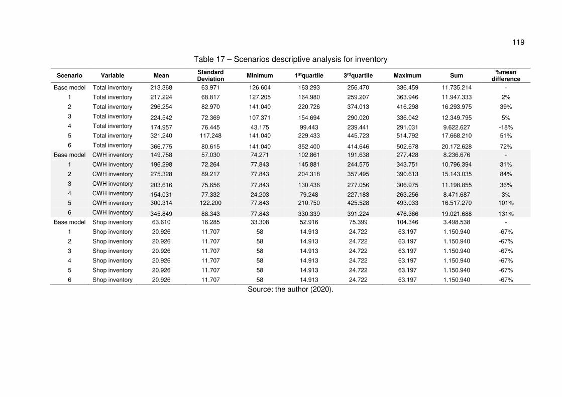
119
Table 17 – Scenarios descriptive analysis for inventory
Scenario Variable Mean Standard Deviation
Minimum 1stquartile 3rdquartile Maximum Sum %mean
difference
Base model Total inventory 213.368 63.971 126.604 163.293 256.470 336.459 11.735.214 -
1 Total inventory 217.224 68.817 127.205 164.980 259.207 363.946 11.947.333 2%
2 Total inventory 296.254 82.970 141.040 220.726 374.013 416.298 16.293.975 39%
3 Total inventory 224.542 72.369 107.371 154.694 290.020 336.042 12.349.795 5% 4 Total inventory 174.957 76.445 43.175 99.443 239.441 291.031 9.622.627 -18% 5 Total inventory 321.240 117.248 141.040 229.433 445.723 514.792 17.668.210 51%
6 Total inventory 366.775 80.615 141.040 352.400 414.646 502.678 20.172.628 72% Base model CWH inventory 149.758 57.030 74.271 102.861 191.638 277.428 8.236.676 -
1 CWH inventory 196.298 72.264 77.843 145.881 244.575 343.751 10.796.394 31%
2 CWH inventory 275.328 89.217 77.843 204.318 357.495 390.613 15.143.035 84%
3 CWH inventory 203.616 75.656 77.843 130.436 277.056 306.975 11.198.855 36% 4 CWH inventory 154.031 77.332 24.203 79.248 227.183 263.256 8.471.687 3% 5 CWH inventory 300.314 122.200 77.843 210.750 425.528 493.033 16.517.270 101%
6 CWH inventory 345.849 88.343 77.843 330.339 391.224 476.366 19.021.688 131% Base model Shop inventory 63.610 16.285 33.308 52.916 75.399 104.346 3.498.538 -
1 Shop inventory 20.926 11.707 58 14.913 24.722 63.197 1.150.940 -67%
2 Shop inventory 20.926 11.707 58 14.913 24.722 63.197 1.150.940 -67%
3 Shop inventory 20.926 11.707 58 14.913 24.722 63.197 1.150.940 -67%
4 Shop inventory 20.926 11.707 58 14.913 24.722 63.197 1.150.940 -67%
5 Shop inventory 20.926 11.707 58 14.913 24.722 63.197 1.150.940 -67%
6 Shop inventory 20.926 11.707 58 14.913 24.722 63.197 1.150.940 -67%
Source: the author (2020).
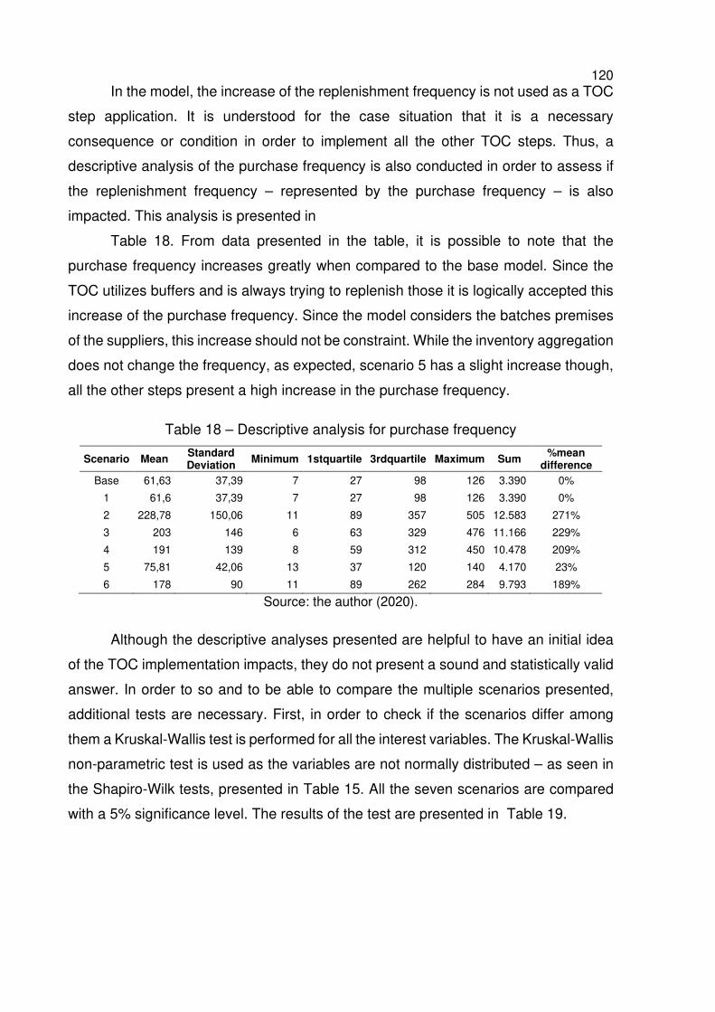
120 In the model, the increase of the replenishment frequency is not used as a TOC
step application. It is understood for the case situation that it is a necessary
consequence or condition in order to implement all the other TOC steps. Thus, a
descriptive analysis of the purchase frequency is also conducted in order to assess if
the replenishment frequency – represented by the purchase frequency – is also
impacted. This analysis is presented in
Table 18. From data presented in the table, it is possible to note that the
purchase frequency increases greatly when compared to the base model. Since the
TOC utilizes buffers and is always trying to replenish those it is logically accepted this
increase of the purchase frequency. Since the model considers the batches premises
of the suppliers, this increase should not be constraint. While the inventory aggregation
does not change the frequency, as expected, scenario 5 has a slight increase though,
all the other steps present a high increase in the purchase frequency.
Table 18 – Descriptive analysis for purchase frequency
Scenario Mean Standard Deviation
Minimum 1stquartile 3rdquartile Maximum Sum %mean
difference
Base 61,63 37,39 7 27 98 126 3.390 0%
1 61,6 37,39 7 27 98 126 3.390 0%
2 228,78 150,06 11 89 357 505 12.583 271%
3 203 146 6 63 329 476 11.166 229%
4 191 139 8 59 312 450 10.478 209%
5 75,81 42,06 13 37 120 140 4.170 23%
6 178 90 11 89 262 284 9.793 189%
Source: the author (2020).
Although the descriptive analyses presented are helpful to have an initial idea
of the TOC implementation impacts, they do not present a sound and statistically valid
answer. In order to so and to be able to compare the multiple scenarios presented,
additional tests are necessary. First, in order to check if the scenarios differ among
them a Kruskal-Wallis test is performed for all the interest variables. The Kruskal-Wallis
non-parametric test is used as the variables are not normally distributed – as seen in
the Shapiro-Wilk tests, presented in Table 15. All the seven scenarios are compared
with a 5% significance level. The results of the test are presented in Table 19.
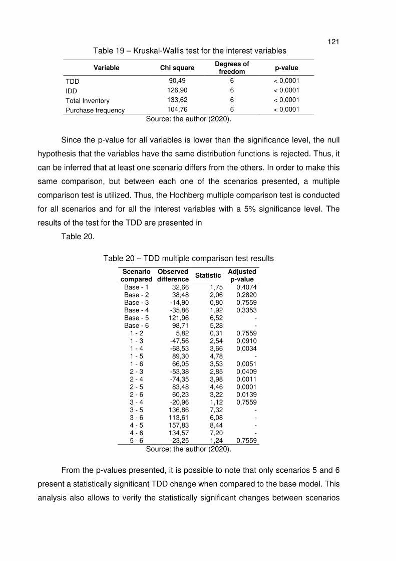
121 Table 19 – Kruskal-Wallis test for the interest variables
Variable Chi square Degrees of
freedom p-value
TDD 90,49 6 < 0,0001
IDD 126,90 6 < 0,0001
Total Inventory 133,62 6 < 0,0001
Purchase frequency 104,76 6 < 0,0001
Source: the author (2020).
Since the p-value for all variables is lower than the significance level, the null
hypothesis that the variables have the same distribution functions is rejected. Thus, it
can be inferred that at least one scenario differs from the others. In order to make this
same comparison, but between each one of the scenarios presented, a multiple
comparison test is utilized. Thus, the Hochberg multiple comparison test is conducted
for all scenarios and for all the interest variables with a 5% significance level. The
results of the test for the TDD are presented in
Table 20.
Table 20 – TDD multiple comparison test results
Scenario compared
Observed difference
Statistic Adjusted p-value
Base - 1 32,66 1,75 0,4074 Base - 2 38,48 2,06 0,2820 Base - 3 -14,90 0,80 0,7559 Base - 4 -35,86 1,92 0,3353 Base - 5 121,96 6,52 - Base - 6 98,71 5,28 -
1 - 2 5,82 0,31 0,7559 1 - 3 -47,56 2,54 0,0910 1 - 4 -68,53 3,66 0,0034 1 - 5 89,30 4,78 - 1 - 6 66,05 3,53 0,0051 2 - 3 -53,38 2,85 0,0409 2 - 4 -74,35 3,98 0,0011 2 - 5 83,48 4,46 0,0001 2 - 6 60,23 3,22 0,0139 3 - 4 -20,96 1,12 0,7559 3 - 5 136,86 7,32 - 3 - 6 113,61 6,08 - 4 - 5 157,83 8,44 - 4 - 6 134,57 7,20 - 5 - 6 -23,25 1,24 0,7559
Source: the author (2020).
From the p-values presented, it is possible to note that only scenarios 5 and 6
present a statistically significant TDD change when compared to the base model. This
analysis also allows to verify the statistically significant changes between scenarios
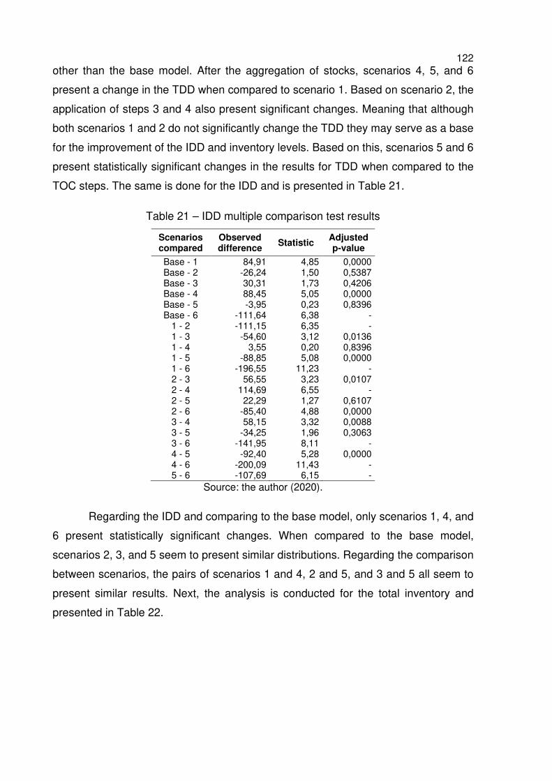
122 other than the base model. After the aggregation of stocks, scenarios 4, 5, and 6
present a change in the TDD when compared to scenario 1. Based on scenario 2, the
application of steps 3 and 4 also present significant changes. Meaning that although
both scenarios 1 and 2 do not significantly change the TDD they may serve as a base
for the improvement of the IDD and inventory levels. Based on this, scenarios 5 and 6
present statistically significant changes in the results for TDD when compared to the
TOC steps. The same is done for the IDD and is presented in Table 21.
Table 21 – IDD multiple comparison test results
Scenarios compared
Observed difference
Statistic Adjusted p-value
Base - 1 84,91 4,85 0,0000 Base - 2 -26,24 1,50 0,5387 Base - 3 30,31 1,73 0,4206 Base - 4 88,45 5,05 0,0000 Base - 5 -3,95 0,23 0,8396 Base - 6 -111,64 6,38 -
1 - 2 -111,15 6,35 - 1 - 3 -54,60 3,12 0,0136 1 - 4 3,55 0,20 0,8396 1 - 5 -88,85 5,08 0,0000 1 - 6 -196,55 11,23 - 2 - 3 56,55 3,23 0,0107 2 - 4 114,69 6,55 - 2 - 5 22,29 1,27 0,6107 2 - 6 -85,40 4,88 0,0000 3 - 4 58,15 3,32 0,0088 3 - 5 -34,25 1,96 0,3063 3 - 6 -141,95 8,11 - 4 - 5 -92,40 5,28 0,0000 4 - 6 -200,09 11,43 - 5 - 6 -107,69 6,15 -
Source: the author (2020).
Regarding the IDD and comparing to the base model, only scenarios 1, 4, and
6 present statistically significant changes. When compared to the base model,
scenarios 2, 3, and 5 seem to present similar distributions. Regarding the comparison
between scenarios, the pairs of scenarios 1 and 4, 2 and 5, and 3 and 5 all seem to
present similar results. Next, the analysis is conducted for the total inventory and
presented in Table 22.
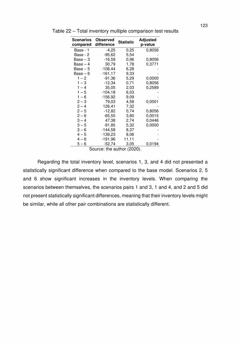
123 Table 22 – Total inventory multiple comparison test results
Scenarios compared
Observed difference
Statistic Adjusted p-value
Base - 1 -4,25 0,25 0,8056 Base - 2 -95,62 5,54 - Base – 3 -16,59 0,96 0,8056 Base – 4 30,79 1,78 0,3771 Base – 5 -108,44 6,28 - Base – 6 -161,17 9,33 -
1 – 2 -91,36 5,29 0,0000 1 – 3 -12,34 0,71 0,8056 1 – 4 35,05 2,03 0,2589 1 – 5 -104,18 6,03 - 1 – 6 -156,92 9,09 - 2 – 3 79,03 4,58 0,0001 2 – 4 126,41 7,32 - 2 – 5 -12,82 0,74 0,8056 2 – 6 -65,55 3,80 0,0015 3 – 4 47,38 2,74 0,0446 3 – 5 -91,85 5,32 0,0000 3 – 6 -144,58 8,37 - 4 – 5 -139,23 8,06 - 4 – 6 -191,96 11,11 - 5 – 6 -52,74 3,05 0,0194
Source: the author (2020).
Regarding the total inventory level, scenarios 1, 3, and 4 did not presented a
statistically significant difference when compared to the base model. Scenarios 2, 5
and 6 show significant increases in the inventory levels. When comparing the
scenarios between themselves, the scenarios pairs 1 and 3, 1 and 4, and 2 and 5 did
not present statistically significant differences, meaning that their inventory levels might
be similar, while all other pair combinations are statistically different.
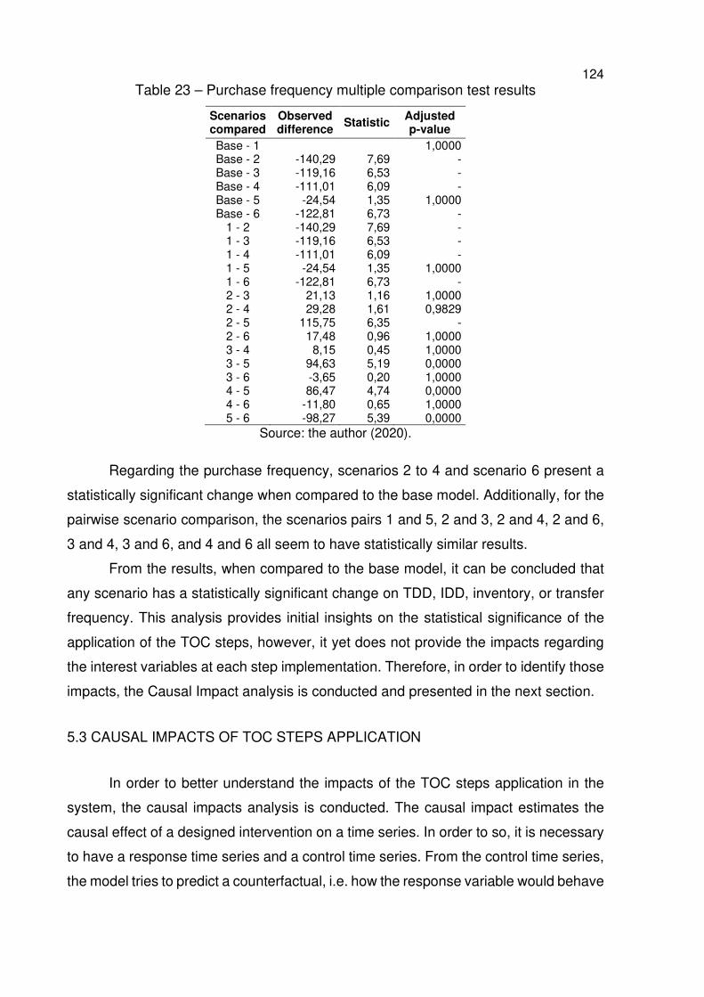
124 Table 23 – Purchase frequency multiple comparison test results
Scenarios compared
Observed difference
Statistic Adjusted p-value
Base - 1 1,0000 Base - 2 -140,29 7,69 - Base - 3 -119,16 6,53 - Base - 4 -111,01 6,09 - Base - 5 -24,54 1,35 1,0000 Base - 6 -122,81 6,73 -
1 - 2 -140,29 7,69 - 1 - 3 -119,16 6,53 - 1 - 4 -111,01 6,09 - 1 - 5 -24,54 1,35 1,0000 1 - 6 -122,81 6,73 - 2 - 3 21,13 1,16 1,0000 2 - 4 29,28 1,61 0,9829 2 - 5 115,75 6,35 - 2 - 6 17,48 0,96 1,0000 3 - 4 8,15 0,45 1,0000 3 - 5 94,63 5,19 0,0000 3 - 6 -3,65 0,20 1,0000 4 - 5 86,47 4,74 0,0000 4 - 6 -11,80 0,65 1,0000 5 - 6 -98,27 5,39 0,0000
Source: the author (2020).
Regarding the purchase frequency, scenarios 2 to 4 and scenario 6 present a
statistically significant change when compared to the base model. Additionally, for the
pairwise scenario comparison, the scenarios pairs 1 and 5, 2 and 3, 2 and 4, 2 and 6,
3 and 4, 3 and 6, and 4 and 6 all seem to have statistically similar results.
From the results, when compared to the base model, it can be concluded that
any scenario has a statistically significant change on TDD, IDD, inventory, or transfer
frequency. This analysis provides initial insights on the statistical significance of the
application of the TOC steps, however, it yet does not provide the impacts regarding
the interest variables at each step implementation. Therefore, in order to identify those
impacts, the Causal Impact analysis is conducted and presented in the next section.
5.3 CAUSAL IMPACTS OF TOC STEPS APPLICATION
In order to better understand the impacts of the TOC steps application in the
system, the causal impacts analysis is conducted. The causal impact estimates the
causal effect of a designed intervention on a time series. In order to so, it is necessary
to have a response time series and a control time series. From the control time series,
the model tries to predict a counterfactual, i.e. how the response variable would behave
125 if the intervention had not occurred. Also, it is important to know when the intervention
takes place, delimiting the pre intervention and the post intervention period. The first
analysis observes the impacts comparing the scenarios to the base model.
5.3.1 Impacts with Regards to the Base Model
The first scenario to be analyzed is the stock aggregation. Therefore, the
interest variables averages through time are compared. Figure 36 presents the
comparison between the base model and scenario 1. The figure presents the results
for TDD in a), IDD in b), total inventory in c), and purchase frequency in d). The solid
blue line represents the time where the intervention takes place in the system, which
is at time 55. Thus, before the blue line are the results of the base model – from time
1 to 55 – and after the line are the results found in the respective scenario – from time
56 to 110. From the figure, it is possible to note the positive impact in both TDD and
IDD from the application of the inventory aggregation. The total inventory no noticeable
changes, and the purchase frequency stays the same, as expected.
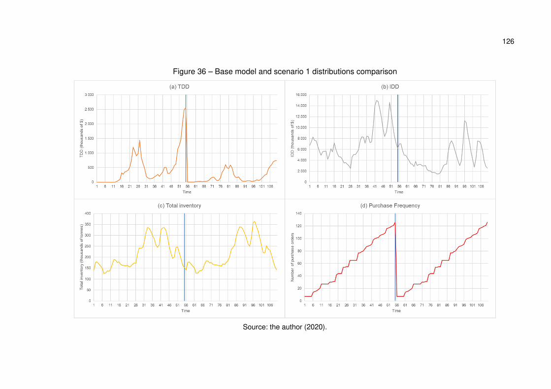
126
Figure 36 – Base model and scenario 1 distributions comparison
Source: the author (2020).
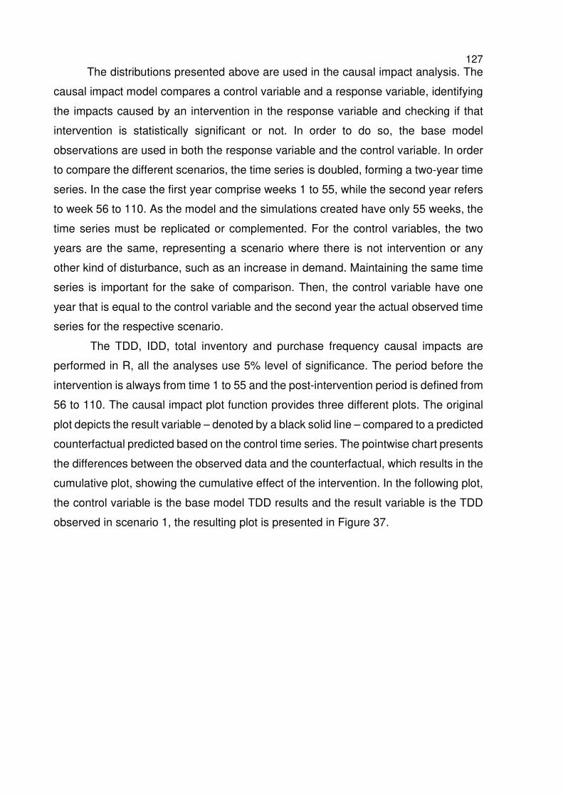
127 The distributions presented above are used in the causal impact analysis. The
causal impact model compares a control variable and a response variable, identifying
the impacts caused by an intervention in the response variable and checking if that
intervention is statistically significant or not. In order to do so, the base model
observations are used in both the response variable and the control variable. In order
to compare the different scenarios, the time series is doubled, forming a two-year time
series. In the case the first year comprise weeks 1 to 55, while the second year refers
to week 56 to 110. As the model and the simulations created have only 55 weeks, the
time series must be replicated or complemented. For the control variables, the two
years are the same, representing a scenario where there is not intervention or any
other kind of disturbance, such as an increase in demand. Maintaining the same time
series is important for the sake of comparison. Then, the control variable have one
year that is equal to the control variable and the second year the actual observed time
series for the respective scenario.
The TDD, IDD, total inventory and purchase frequency causal impacts are
performed in R, all the analyses use 5% level of significance. The period before the
intervention is always from time 1 to 55 and the post-intervention period is defined from
56 to 110. The causal impact plot function provides three different plots. The original
plot depicts the result variable – denoted by a black solid line – compared to a predicted
counterfactual predicted based on the control time series. The pointwise chart presents
the differences between the observed data and the counterfactual, which results in the
cumulative plot, showing the cumulative effect of the intervention. In the following plot,
the control variable is the base model TDD results and the result variable is the TDD
observed in scenario 1, the resulting plot is presented in Figure 37.
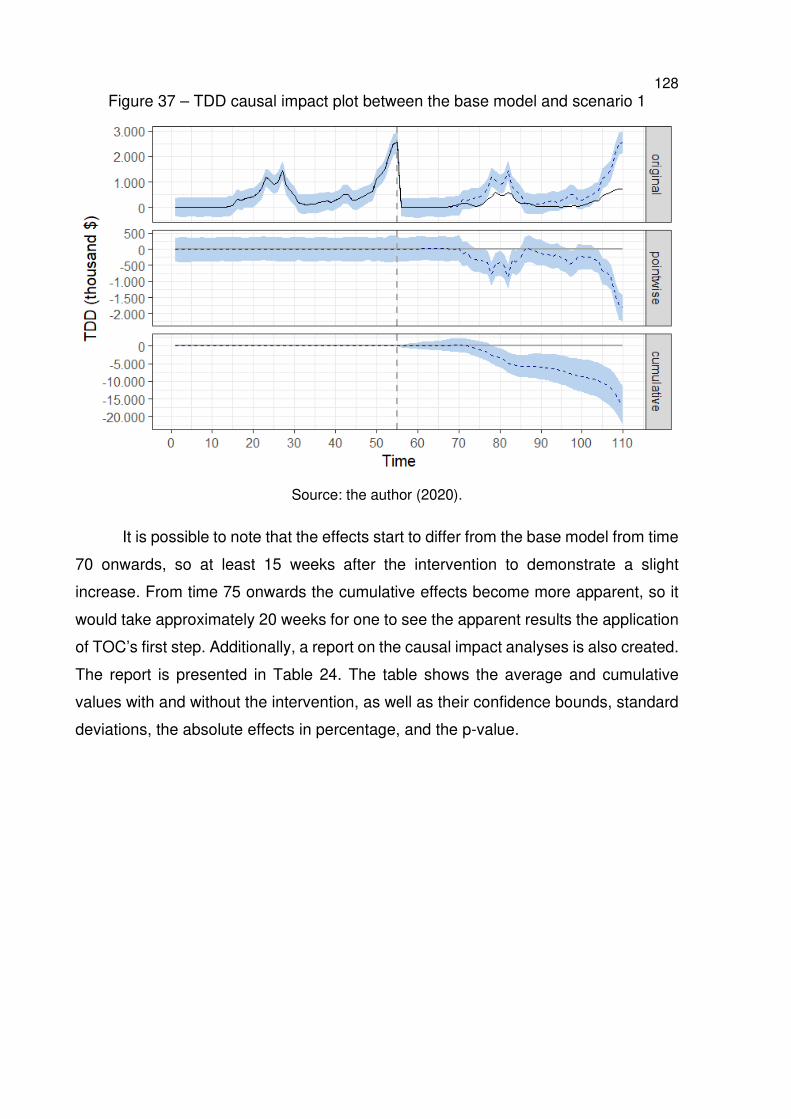
128 Figure 37 – TDD causal impact plot between the base model and scenario 1
Source: the author (2020).
It is possible to note that the effects start to differ from the base model from time
70 onwards, so at least 15 weeks after the intervention to demonstrate a slight
increase. From time 75 onwards the cumulative effects become more apparent, so it
would take approximately 20 weeks for one to see the apparent results the application
of TOC’s first step. Additionally, a report on the causal impact analyses is also created.
The report is presented in Table 24. The table shows the average and cumulative
values with and without the intervention, as well as their confidence bounds, standard
deviations, the absolute effects in percentage, and the p-value.
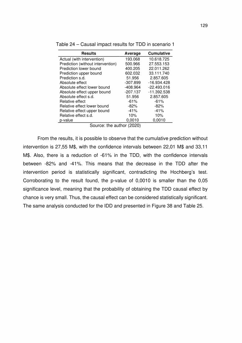
129
Table 24 – Causal impact results for TDD in scenario 1
Results Average Cumulative
Actual (with intervention) 193.068 10.618.725 Prediction (without intervention) 500.966 27.553.153 Prediction lower bound 400.205 22.011.262 Prediction upper bound 602.032 33.111.740 Prediction s.d. 51.956 2.857.605 Absolute effect -307.899 -16.934.428 Absolute effect lower bound -408.964 -22.493.016 Absolute effect upper bound -207.137 -11.392.538 Absolute effect s.d. 51.956 2.857.605 Relative effect -61% -61% Relative effect lower bound -82% -82% Relative effect upper bound -41% -41% Relative effect s.d. 10% 10% p-value 0,0010 0,0010
Source: the author (2020)
From the results, it is possible to observe that the cumulative prediction without
intervention is 27,55 M$, with the confidence intervals between 22,01 M$ and 33,11
M$. Also, there is a reduction of -61% in the TDD, with the confidence intervals
between -82% and -41%. This means that the decrease in the TDD after the
intervention period is statistically significant, contradicting the Hochberg’s test.
Corroborating to the result found, the p-value of 0,0010 is smaller than the 0,05
significance level, meaning that the probability of obtaining the TDD causal effect by
chance is very small. Thus, the causal effect can be considered statistically significant.
The same analysis conducted for the IDD and presented in Figure 38 and Table 25.
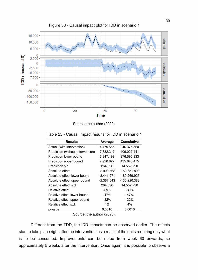
130 Figure 38 - Causal impact plot for IDD in scenario 1
Source: the author (2020).
Table 25 - Causal Impact results for IDD in scenario 1
Results Average Cumulative
Actual (with intervention) 4.479.555 246.375.550 Prediction (without intervention) 7.382.317 406.027.441 Prediction lower bound 6.847.199 376.595.933 Prediction upper bound 7.920.827 435.645.475 Prediction s.d. 264.596 14.552.790 Absolute effect -2.902.762 -159.651.892 Absolute effect lower bound -3.441.271 -189.269.925 Absolute effect upper bound -2.367.643 -130.220.383 Absolute effect s.d. 264.596 14.552.790 Relative effect -39% -39% Relative effect lower bound -47% -47% Relative effect upper bound -32% -32% Relative effect s.d. 4% 4%
p-value 0,0010 0,0010
Source: the author (2020).
Different from the TDD, the IDD impacts can be observed earlier. The effects
start to take place right after the intervention, as a result of the units requiring only what
is to be consumed. Improvements can be noted from week 60 onwards, so
approximately 5 weeks after the intervention. Once again, it is possible to observe a
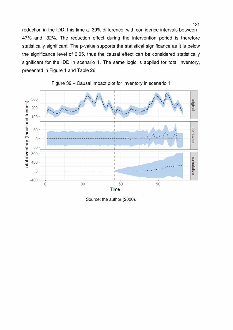
131 reduction in the IDD, this time a -39% difference, with confidence intervals between -
47% and -32%. The reduction effect during the intervention period is therefore
statistically significant. The p-value supports the statistical significance as it is below
the significance level of 0,05, thus the causal effect can be considered statistically
significant for the IDD in scenario 1. The same logic is applied for total inventory,
presented in Figure 1 and Table 26.
Figure 39 – Causal impact plot for inventory in scenario 1
Source: the author (2020).
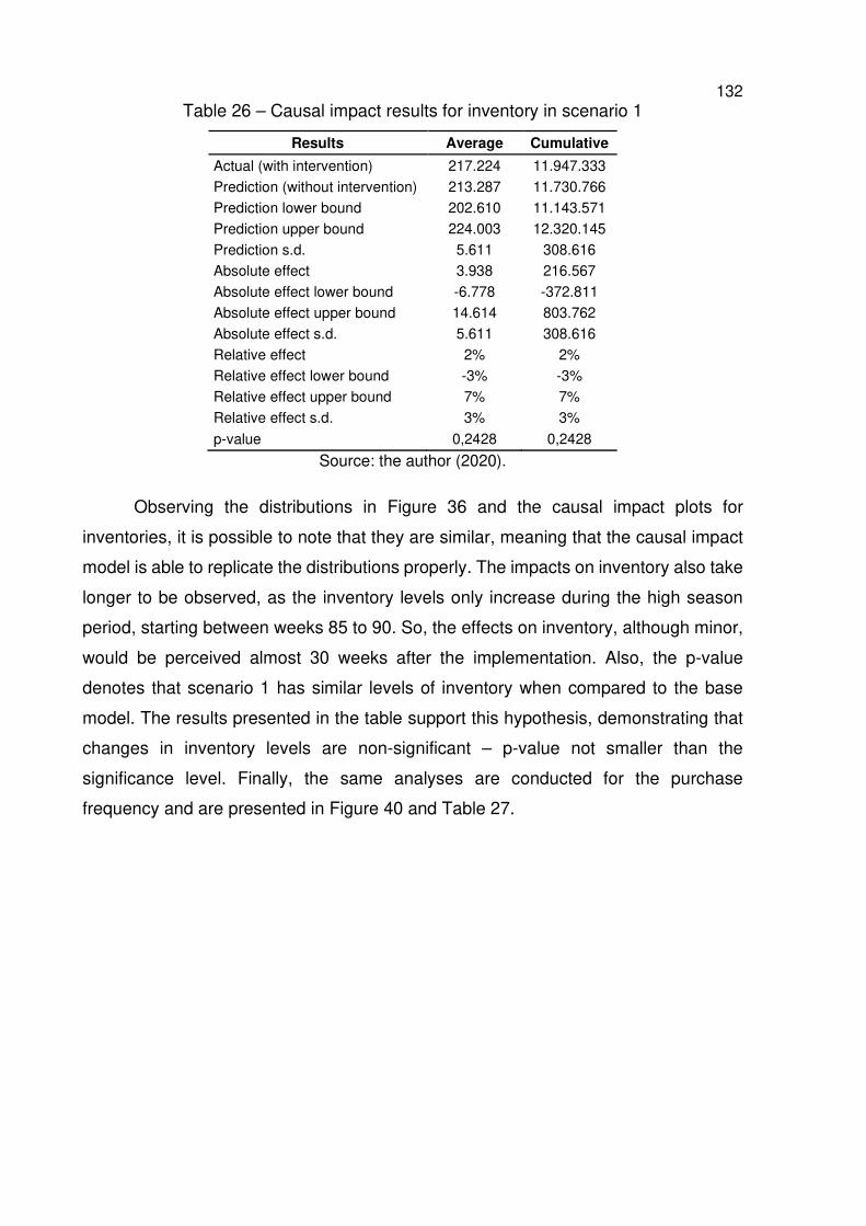
132 Table 26 – Causal impact results for inventory in scenario 1
Results Average Cumulative
Actual (with intervention) 217.224 11.947.333 Prediction (without intervention) 213.287 11.730.766 Prediction lower bound 202.610 11.143.571 Prediction upper bound 224.003 12.320.145 Prediction s.d. 5.611 308.616 Absolute effect 3.938 216.567 Absolute effect lower bound -6.778 -372.811 Absolute effect upper bound 14.614 803.762 Absolute effect s.d. 5.611 308.616 Relative effect 2% 2% Relative effect lower bound -3% -3% Relative effect upper bound 7% 7% Relative effect s.d. 3% 3%
p-value 0,2428 0,2428
Source: the author (2020).
Observing the distributions in Figure 36 and the causal impact plots for
inventories, it is possible to note that they are similar, meaning that the causal impact
model is able to replicate the distributions properly. The impacts on inventory also take
longer to be observed, as the inventory levels only increase during the high season
period, starting between weeks 85 to 90. So, the effects on inventory, although minor,
would be perceived almost 30 weeks after the implementation. Also, the p-value
denotes that scenario 1 has similar levels of inventory when compared to the base
model. The results presented in the table support this hypothesis, demonstrating that
changes in inventory levels are non-significant – p-value not smaller than the
significance level. Finally, the same analyses are conducted for the purchase
frequency and are presented in Figure 40 and Table 27.
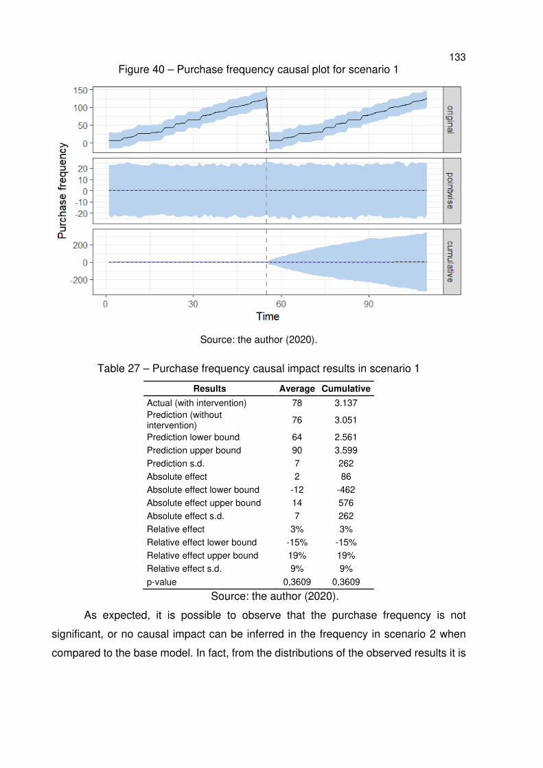
133 Figure 40 – Purchase frequency causal plot for scenario 1
Source: the author (2020).
Table 27 – Purchase frequency causal impact results in scenario 1
Results Average Cumulative
Actual (with intervention) 78 3.137 Prediction (without intervention) 76 3.051
Prediction lower bound 64 2.561 Prediction upper bound 90 3.599 Prediction s.d. 7 262 Absolute effect 2 86 Absolute effect lower bound -12 -462 Absolute effect upper bound 14 576 Absolute effect s.d. 7 262 Relative effect 3% 3% Relative effect lower bound -15% -15% Relative effect upper bound 19% 19% Relative effect s.d. 9% 9%
p-value 0,3609 0,3609
Source: the author (2020).
As expected, it is possible to observe that the purchase frequency is not
significant, or no causal impact can be inferred in the frequency in scenario 2 when
compared to the base model. In fact, from the distributions of the observed results it is
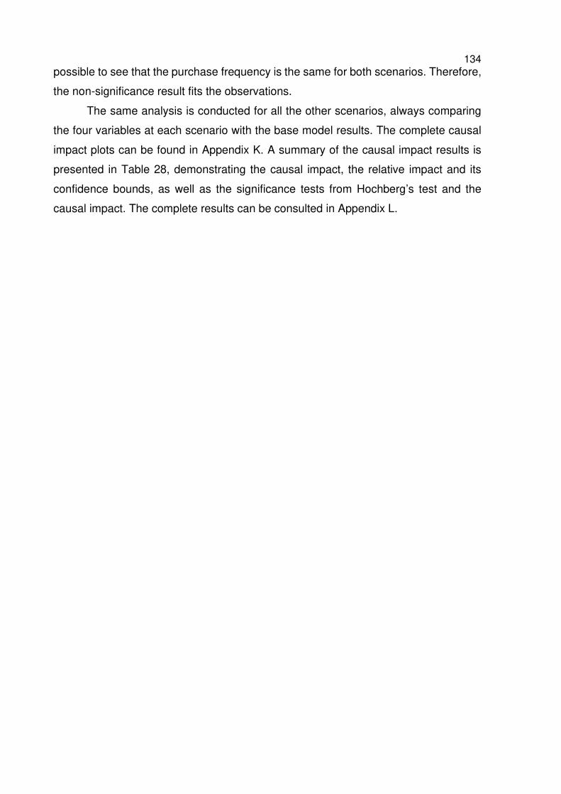
134 possible to see that the purchase frequency is the same for both scenarios. Therefore,
the non-significance result fits the observations.
The same analysis is conducted for all the other scenarios, always comparing
the four variables at each scenario with the base model results. The complete causal
impact plots can be found in Appendix K. A summary of the causal impact results is
presented in Table 28, demonstrating the causal impact, the relative impact and its
confidence bounds, as well as the significance tests from Hochberg’s test and the
causal impact. The complete results can be consulted in Appendix L.
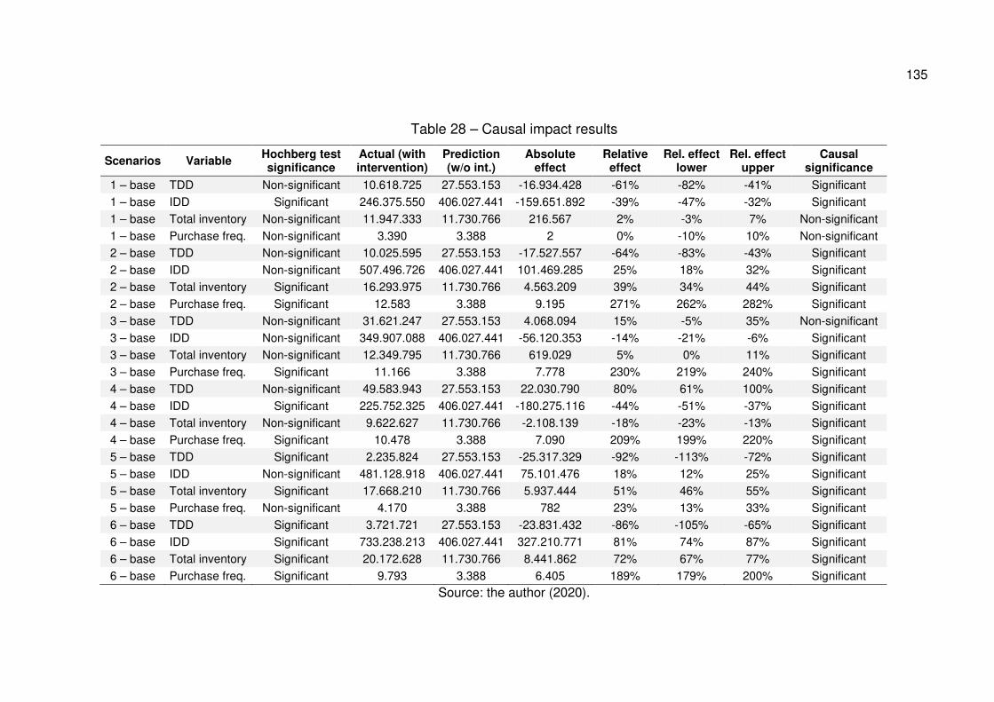
135
Table 28 – Causal impact results
Scenarios Variable Hochberg test significance
Actual (with intervention)
Prediction (w/o int.)
Absolute effect
Relative effect
Rel. effect lower
Rel. effect upper
Causal significance
1 – base TDD Non-significant 10.618.725 27.553.153 -16.934.428 -61% -82% -41% Significant 1 – base IDD Significant 246.375.550 406.027.441 -159.651.892 -39% -47% -32% Significant 1 – base Total inventory Non-significant 11.947.333 11.730.766 216.567 2% -3% 7% Non-significant 1 – base Purchase freq. Non-significant 3.390 3.388 2 0% -10% 10% Non-significant 2 – base TDD Non-significant 10.025.595 27.553.153 -17.527.557 -64% -83% -43% Significant 2 – base IDD Non-significant 507.496.726 406.027.441 101.469.285 25% 18% 32% Significant 2 – base Total inventory Significant 16.293.975 11.730.766 4.563.209 39% 34% 44% Significant 2 – base Purchase freq. Significant 12.583 3.388 9.195 271% 262% 282% Significant 3 – base TDD Non-significant 31.621.247 27.553.153 4.068.094 15% -5% 35% Non-significant 3 – base IDD Non-significant 349.907.088 406.027.441 -56.120.353 -14% -21% -6% Significant 3 – base Total inventory Non-significant 12.349.795 11.730.766 619.029 5% 0% 11% Significant 3 – base Purchase freq. Significant 11.166 3.388 7.778 230% 219% 240% Significant 4 – base TDD Non-significant 49.583.943 27.553.153 22.030.790 80% 61% 100% Significant 4 – base IDD Significant 225.752.325 406.027.441 -180.275.116 -44% -51% -37% Significant 4 – base Total inventory Non-significant 9.622.627 11.730.766 -2.108.139 -18% -23% -13% Significant 4 – base Purchase freq. Significant 10.478 3.388 7.090 209% 199% 220% Significant 5 – base TDD Significant 2.235.824 27.553.153 -25.317.329 -92% -113% -72% Significant 5 – base IDD Non-significant 481.128.918 406.027.441 75.101.476 18% 12% 25% Significant 5 – base Total inventory Significant 17.668.210 11.730.766 5.937.444 51% 46% 55% Significant 5 – base Purchase freq. Non-significant 4.170 3.388 782 23% 13% 33% Significant 6 – base TDD Significant 3.721.721 27.553.153 -23.831.432 -86% -105% -65% Significant 6 – base IDD Significant 733.238.213 406.027.441 327.210.771 81% 74% 87% Significant 6 – base Total inventory Significant 20.172.628 11.730.766 8.441.862 72% 67% 77% Significant 6 – base Purchase freq. Significant 9.793 3.388 6.405 189% 179% 200% Significant
Source: the author (2020).
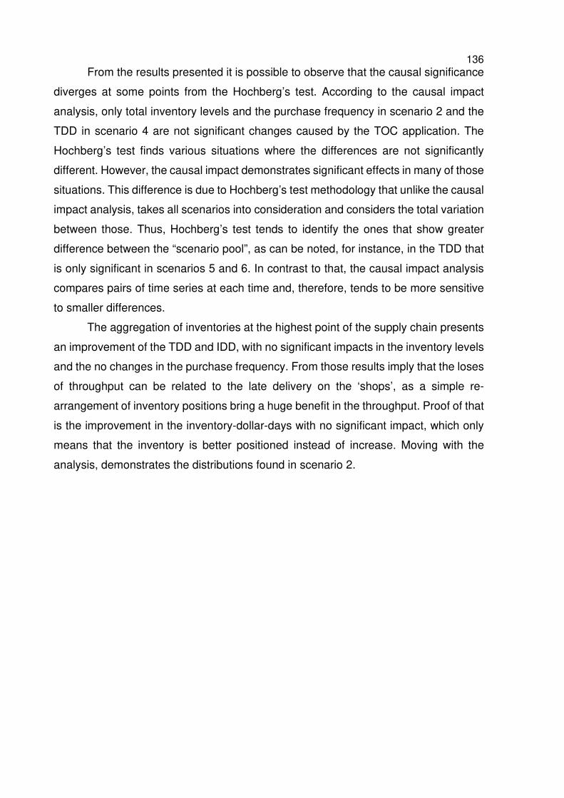
136 From the results presented it is possible to observe that the causal significance
diverges at some points from the Hochberg’s test. According to the causal impact
analysis, only total inventory levels and the purchase frequency in scenario 2 and the
TDD in scenario 4 are not significant changes caused by the TOC application. The
Hochberg’s test finds various situations where the differences are not significantly
different. However, the causal impact demonstrates significant effects in many of those
situations. This difference is due to Hochberg’s test methodology that unlike the causal
impact analysis, takes all scenarios into consideration and considers the total variation
between those. Thus, Hochberg’s test tends to identify the ones that show greater
difference between the “scenario pool”, as can be noted, for instance, in the TDD that
is only significant in scenarios 5 and 6. In contrast to that, the causal impact analysis
compares pairs of time series at each time and, therefore, tends to be more sensitive
to smaller differences.
The aggregation of inventories at the highest point of the supply chain presents
an improvement of the TDD and IDD, with no significant impacts in the inventory levels
and the no changes in the purchase frequency. From those results imply that the loses
of throughput can be related to the late delivery on the ‘shops’, as a simple re-
arrangement of inventory positions bring a huge benefit in the throughput. Proof of that
is the improvement in the inventory-dollar-days with no significant impact, which only
means that the inventory is better positioned instead of increase. Moving with the
analysis, demonstrates the distributions found in scenario 2.
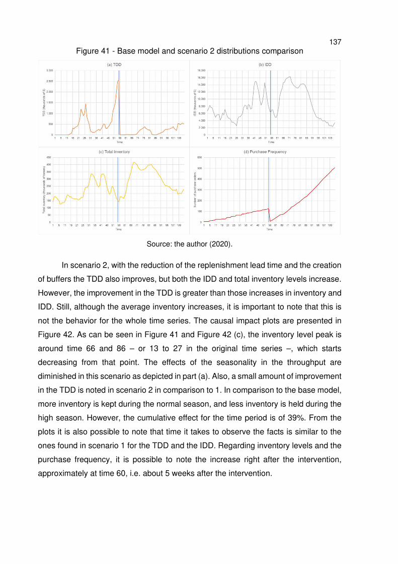
137 Figure 41 - Base model and scenario 2 distributions comparison
Source: the author (2020).
In scenario 2, with the reduction of the replenishment lead time and the creation
of buffers the TDD also improves, but both the IDD and total inventory levels increase.
However, the improvement in the TDD is greater than those increases in inventory and
IDD. Still, although the average inventory increases, it is important to note that this is
not the behavior for the whole time series. The causal impact plots are presented in
Figure 42. As can be seen in Figure 41 and Figure 42 (c), the inventory level peak is
around time 66 and 86 – or 13 to 27 in the original time series –, which starts
decreasing from that point. The effects of the seasonality in the throughput are
diminished in this scenario as depicted in part (a). Also, a small amount of improvement
in the TDD is noted in scenario 2 in comparison to 1. In comparison to the base model,
more inventory is kept during the normal season, and less inventory is held during the
high season. However, the cumulative effect for the time period is of 39%. From the
plots it is also possible to note that time it takes to observe the facts is similar to the
ones found in scenario 1 for the TDD and the IDD. Regarding inventory levels and the
purchase frequency, it is possible to note the increase right after the intervention,
approximately at time 60, i.e. about 5 weeks after the intervention.
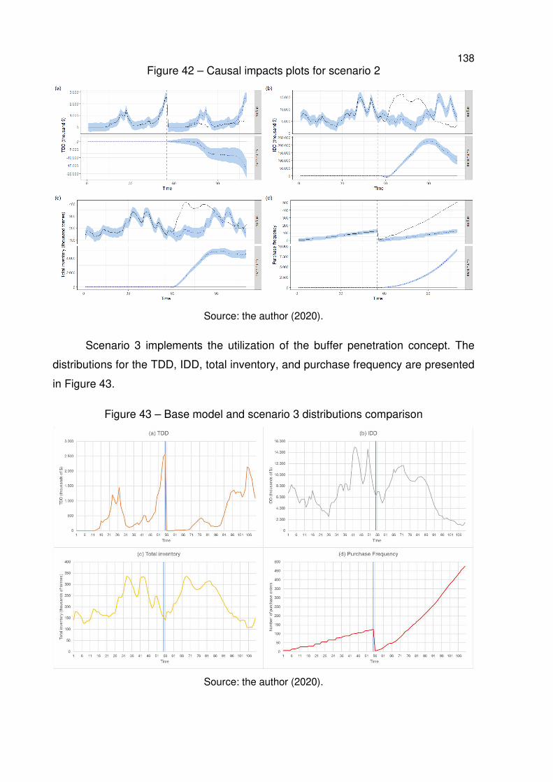
138 Figure 42 – Causal impacts plots for scenario 2
Source: the author (2020).
Scenario 3 implements the utilization of the buffer penetration concept. The
distributions for the TDD, IDD, total inventory, and purchase frequency are presented
in Figure 43.
Figure 43 – Base model and scenario 3 distributions comparison
Source: the author (2020).
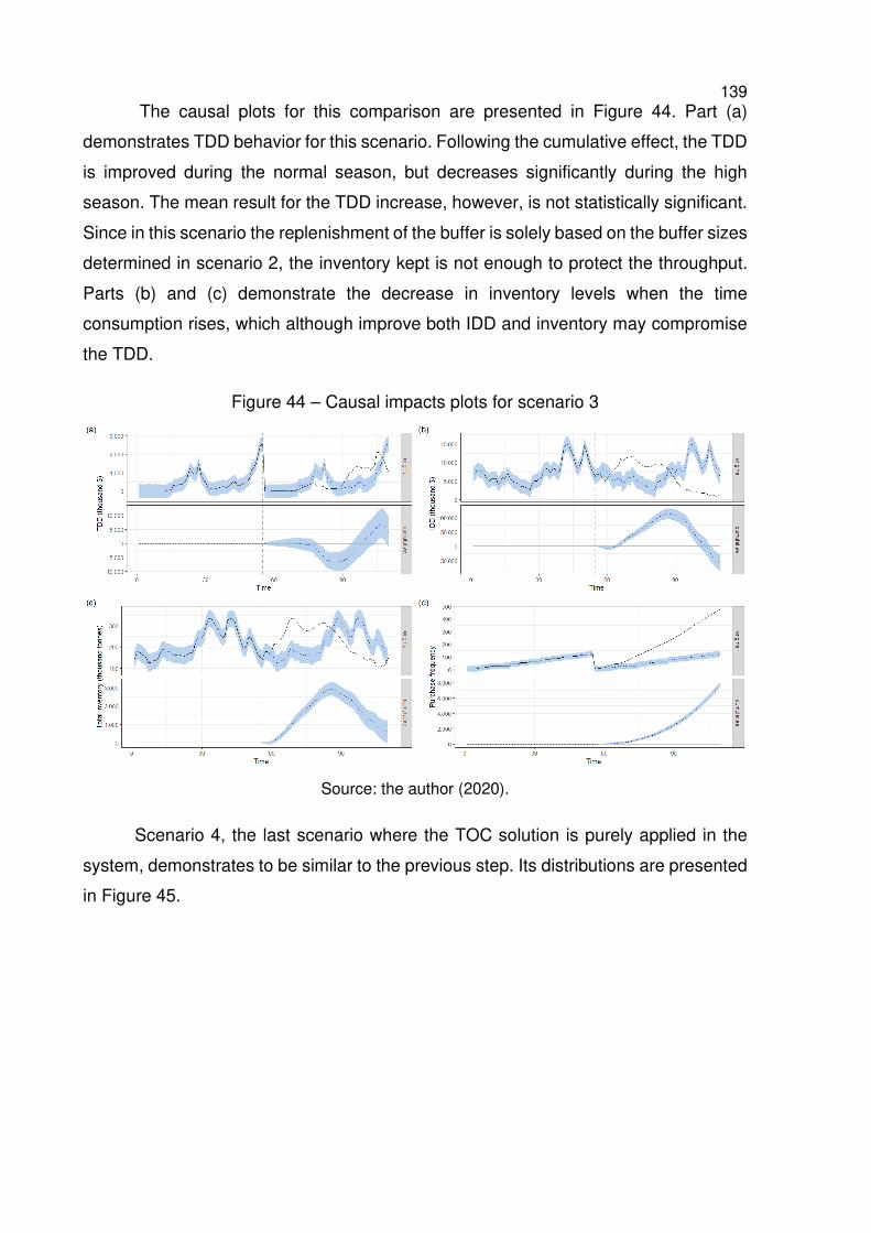
139 The causal plots for this comparison are presented in Figure 44. Part (a)
demonstrates TDD behavior for this scenario. Following the cumulative effect, the TDD
is improved during the normal season, but decreases significantly during the high
season. The mean result for the TDD increase, however, is not statistically significant.
Since in this scenario the replenishment of the buffer is solely based on the buffer sizes
determined in scenario 2, the inventory kept is not enough to protect the throughput.
Parts (b) and (c) demonstrate the decrease in inventory levels when the time
consumption rises, which although improve both IDD and inventory may compromise
the TDD.
Figure 44 – Causal impacts plots for scenario 3
Source: the author (2020).
Scenario 4, the last scenario where the TOC solution is purely applied in the
system, demonstrates to be similar to the previous step. Its distributions are presented
in Figure 45.
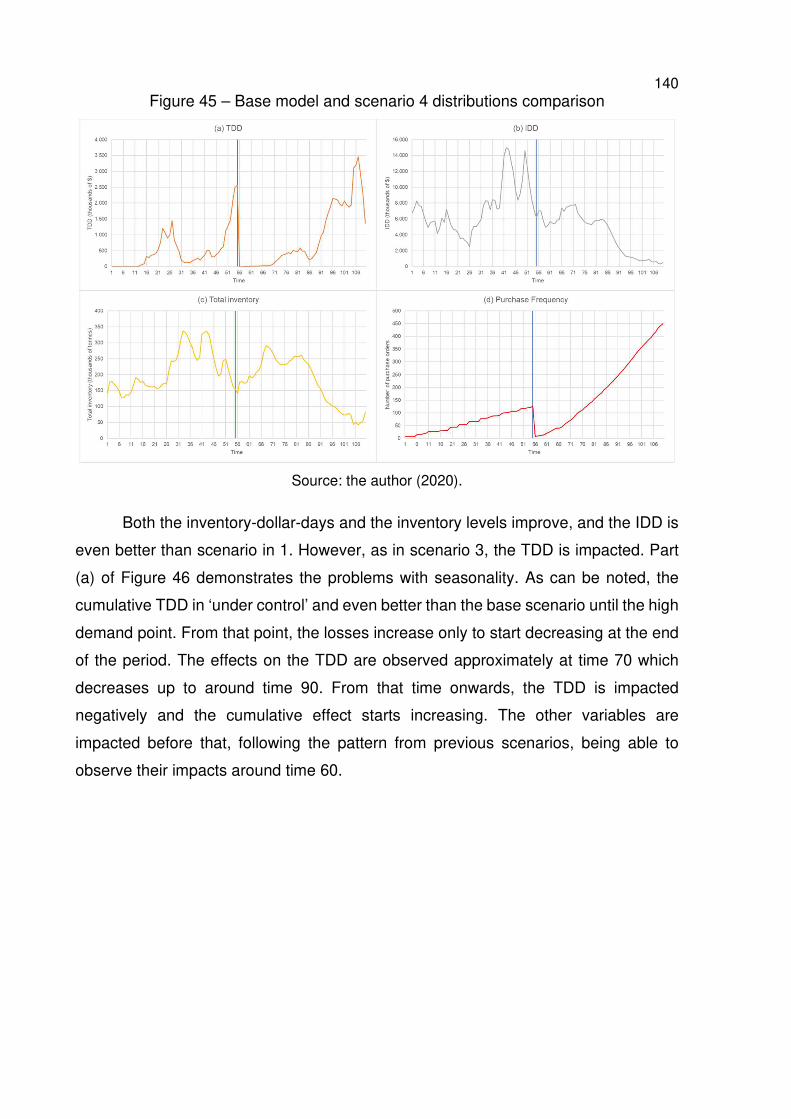
140 Figure 45 – Base model and scenario 4 distributions comparison
Source: the author (2020).
Both the inventory-dollar-days and the inventory levels improve, and the IDD is
even better than scenario in 1. However, as in scenario 3, the TDD is impacted. Part
(a) of Figure 46 demonstrates the problems with seasonality. As can be noted, the
cumulative TDD in ‘under control’ and even better than the base scenario until the high
demand point. From that point, the losses increase only to start decreasing at the end
of the period. The effects on the TDD are observed approximately at time 70 which
decreases up to around time 90. From that time onwards, the TDD is impacted
negatively and the cumulative effect starts increasing. The other variables are
impacted before that, following the pattern from previous scenarios, being able to
observe their impacts around time 60.
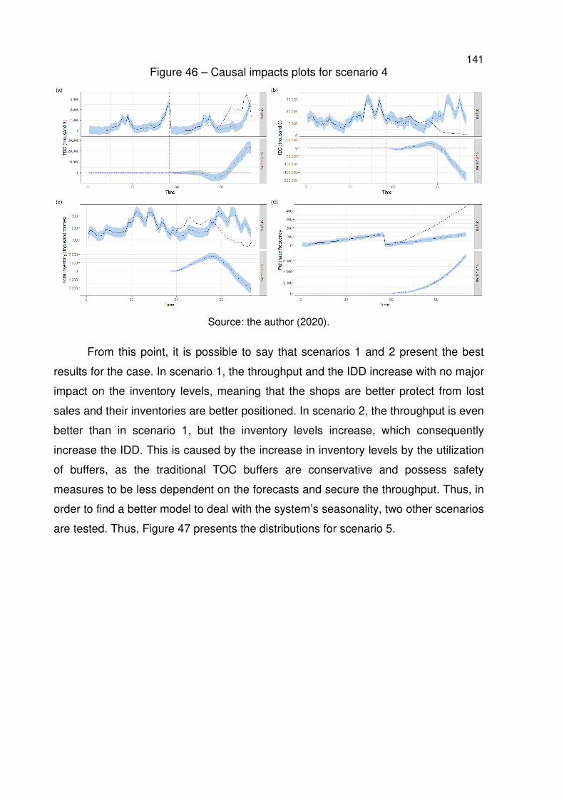
141 Figure 46 – Causal impacts plots for scenario 4
Source: the author (2020).
From this point, it is possible to say that scenarios 1 and 2 present the best
results for the case. In scenario 1, the throughput and the IDD increase with no major
impact on the inventory levels, meaning that the shops are better protect from lost
sales and their inventories are better positioned. In scenario 2, the throughput is even
better than in scenario 1, but the inventory levels increase, which consequently
increase the IDD. This is caused by the increase in inventory levels by the utilization
of buffers, as the traditional TOC buffers are conservative and possess safety
measures to be less dependent on the forecasts and secure the throughput. Thus, in
order to find a better model to deal with the system’s seasonality, two other scenarios
are tested. Thus, Figure 47 presents the distributions for scenario 5.
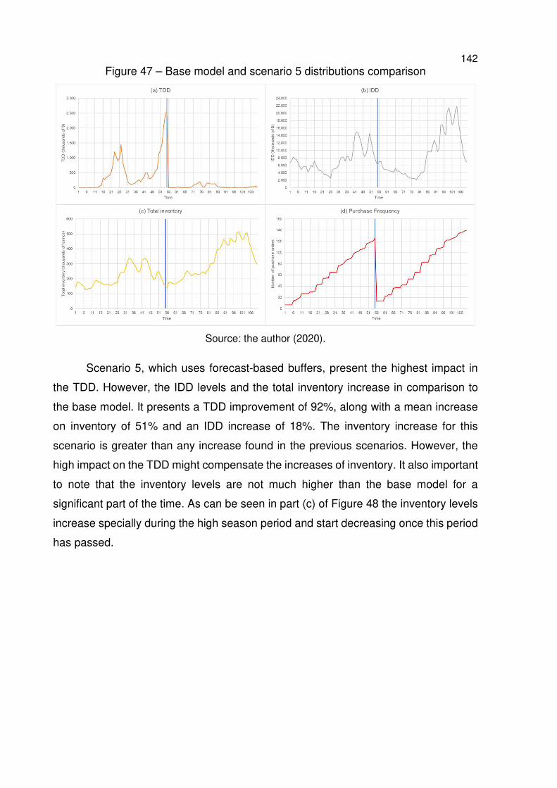
142 Figure 47 – Base model and scenario 5 distributions comparison
Source: the author (2020).
Scenario 5, which uses forecast-based buffers, present the highest impact in
the TDD. However, the IDD levels and the total inventory increase in comparison to
the base model. It presents a TDD improvement of 92%, along with a mean increase
on inventory of 51% and an IDD increase of 18%. The inventory increase for this
scenario is greater than any increase found in the previous scenarios. However, the
high impact on the TDD might compensate the increases of inventory. It also important
to note that the inventory levels are not much higher than the base model for a
significant part of the time. As can be seen in part (c) of Figure 48 the inventory levels
increase specially during the high season period and start decreasing once this period
has passed.
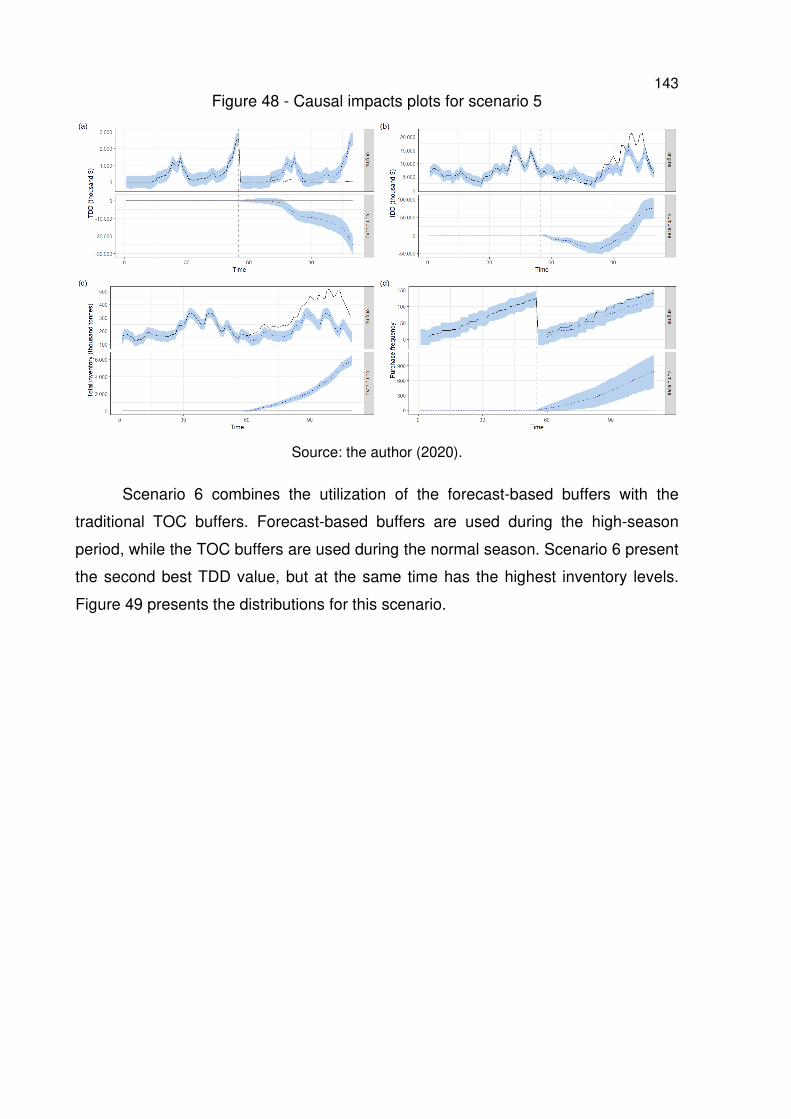
143 Figure 48 - Causal impacts plots for scenario 5
Source: the author (2020).
Scenario 6 combines the utilization of the forecast-based buffers with the
traditional TOC buffers. Forecast-based buffers are used during the high-season
period, while the TOC buffers are used during the normal season. Scenario 6 present
the second best TDD value, but at the same time has the highest inventory levels.
Figure 49 presents the distributions for this scenario.
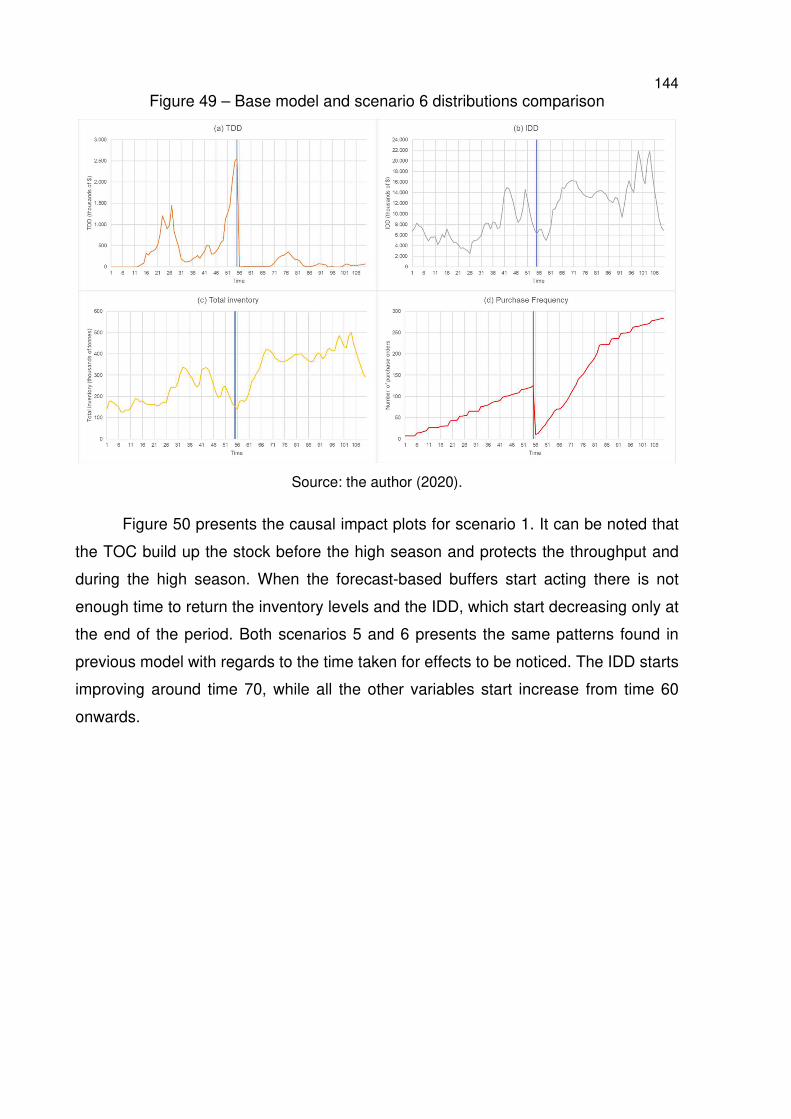
144 Figure 49 – Base model and scenario 6 distributions comparison
Source: the author (2020).
Figure 50 presents the causal impact plots for scenario 1. It can be noted that
the TOC build up the stock before the high season and protects the throughput and
during the high season. When the forecast-based buffers start acting there is not
enough time to return the inventory levels and the IDD, which start decreasing only at
the end of the period. Both scenarios 5 and 6 presents the same patterns found in
previous model with regards to the time taken for effects to be noticed. The IDD starts
improving around time 70, while all the other variables start increase from time 60
onwards.
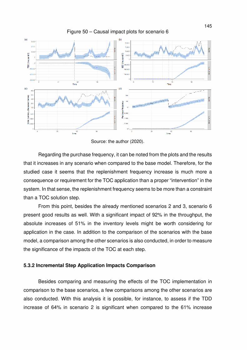
145 Figure 50 – Causal impact plots for scenario 6
Source: the author (2020).
Regarding the purchase frequency, it can be noted from the plots and the results
that it increases in any scenario when compared to the base model. Therefore, for the
studied case it seems that the replenishment frequency increase is much more a
consequence or requirement for the TOC application than a proper “intervention” in the
system. In that sense, the replenishment frequency seems to be more than a constraint
than a TOC solution step.
From this point, besides the already mentioned scenarios 2 and 3, scenario 6
present good results as well. With a significant impact of 92% in the throughput, the
absolute increases of 51% in the inventory levels might be worth considering for
application in the case. In addition to the comparison of the scenarios with the base
model, a comparison among the other scenarios is also conducted, in order to measure
the significance of the impacts of the TOC at each step.
5.3.2 Incremental Step Application Impacts Comparison
Besides comparing and measuring the effects of the TOC implementation in
comparison to the base scenarios, a few comparisons among the other scenarios are
also conducted. With this analysis it is possible, for instance, to assess if the TDD
increase of 64% in scenario 2 is significant when compared to the 61% increase

146 achieved during scenario 1. The aim is to assess each incremental step of the TOC
application, thus the causal impacts between scenarios 1 and 2, 2 and 3, and 3 and 4
will be measured. Additionally, scenarios 5 and 6 are both compared to scenario 4,
which represents the application of the last TOC step. A summary of the results from
the analysis are presented in Table 29. The complete results can be found in Appendix
L. Additionally, the causal plots can be consulted in Appendix K.
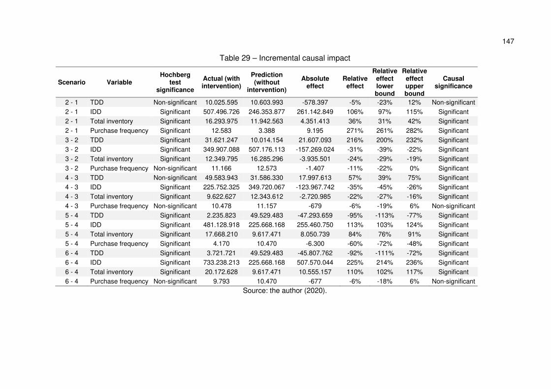
147
Table 29 – Incremental causal impact
Scenario Variable Hochberg
test significance
Actual (with intervention)
Prediction (without
intervention)
Absolute effect
Relative effect
Relative effect lower bound
Relative effect upper bound
Causal significance
2 - 1 TDD Non-significant 10.025.595 10.603.993 -578.397 -5% -23% 12% Non-significant 2 - 1 IDD Significant 507.496.726 246.353.877 261.142.849 106% 97% 115% Significant 2 - 1 Total inventory Significant 16.293.975 11.942.563 4.351.413 36% 31% 42% Significant 2 - 1 Purchase frequency Significant 12.583 3.388 9.195 271% 261% 282% Significant 3 - 2 TDD Significant 31.621.247 10.014.154 21.607.093 216% 200% 232% Significant 3 - 2 IDD Significant 349.907.088 507.176.113 -157.269.024 -31% -39% -22% Significant 3 - 2 Total inventory Significant 12.349.795 16.285.296 -3.935.501 -24% -29% -19% Significant 3 - 2 Purchase frequency Non-significant 11.166 12.573 -1.407 -11% -22% 0% Significant 4 - 3 TDD Non-significant 49.583.943 31.586.330 17.997.613 57% 39% 75% Significant 4 - 3 IDD Significant 225.752.325 349.720.067 -123.967.742 -35% -45% -26% Significant 4 - 3 Total inventory Significant 9.622.627 12.343.612 -2.720.985 -22% -27% -16% Significant 4 - 3 Purchase frequency Non-significant 10.478 11.157 -679 -6% -19% 6% Non-significant 5 - 4 TDD Significant 2.235.823 49.529.483 -47.293.659 -95% -113% -77% Significant 5 - 4 IDD Significant 481.128.918 225.668.168 255.460.750 113% 103% 124% Significant 5 - 4 Total inventory Significant 17.668.210 9.617.471 8.050.739 84% 76% 91% Significant 5 - 4 Purchase frequency Significant 4.170 10.470 -6.300 -60% -72% -48% Significant 6 - 4 TDD Significant 3.721.721 49.529.483 -45.807.762 -92% -111% -72% Significant 6 - 4 IDD Significant 733.238.213 225.668.168 507.570.044 225% 214% 236% Significant 6 - 4 Total inventory Significant 20.172.628 9.617.471 10.555.157 110% 102% 117% Significant 6 - 4 Purchase frequency Non-significant 9.793 10.470 -677 -6% -18% 6% Non-significant
Source: the author (2020).
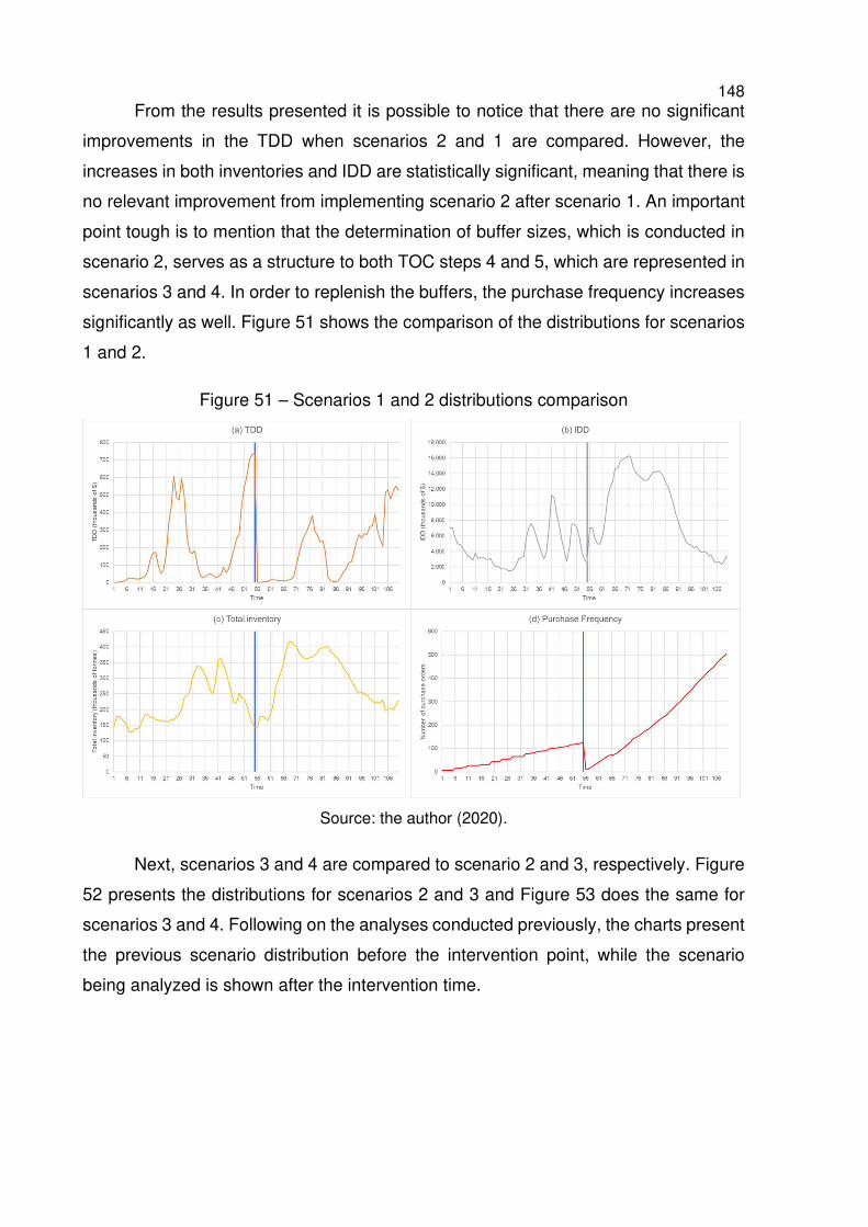
148 From the results presented it is possible to notice that there are no significant
improvements in the TDD when scenarios 2 and 1 are compared. However, the
increases in both inventories and IDD are statistically significant, meaning that there is
no relevant improvement from implementing scenario 2 after scenario 1. An important
point tough is to mention that the determination of buffer sizes, which is conducted in
scenario 2, serves as a structure to both TOC steps 4 and 5, which are represented in
scenarios 3 and 4. In order to replenish the buffers, the purchase frequency increases
significantly as well. Figure 51 shows the comparison of the distributions for scenarios
1 and 2.
Figure 51 – Scenarios 1 and 2 distributions comparison
Source: the author (2020).
Next, scenarios 3 and 4 are compared to scenario 2 and 3, respectively. Figure
52 presents the distributions for scenarios 2 and 3 and Figure 53 does the same for
scenarios 3 and 4. Following on the analyses conducted previously, the charts present
the previous scenario distribution before the intervention point, while the scenario
being analyzed is shown after the intervention time.
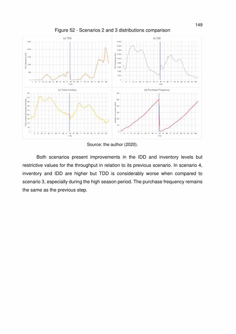
149 Figure 52 - Scenarios 2 and 3 distributions comparison
Source: the author (2020).
Both scenarios present improvements in the IDD and inventory levels but
restrictive values for the throughput in relation to its previous scenario. In scenario 4,
inventory and IDD are higher but TDD is considerably worse when compared to
scenario 3, especially during the high season period. The purchase frequency remains
the same as the previous step.
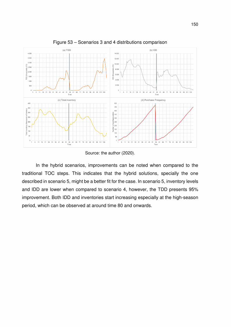
150
Figure 53 – Scenarios 3 and 4 distributions comparison
Source: the author (2020).
In the hybrid scenarios, improvements can be noted when compared to the
traditional TOC steps. This indicates that the hybrid solutions, specially the one
described in scenario 5, might be a better fit for the case. In scenario 5, inventory levels
and IDD are lower when compared to scenario 4, however, the TDD presents 95%
improvement. Both IDD and inventories start increasing especially at the high-season
period, which can be observed at around time 80 and onwards.
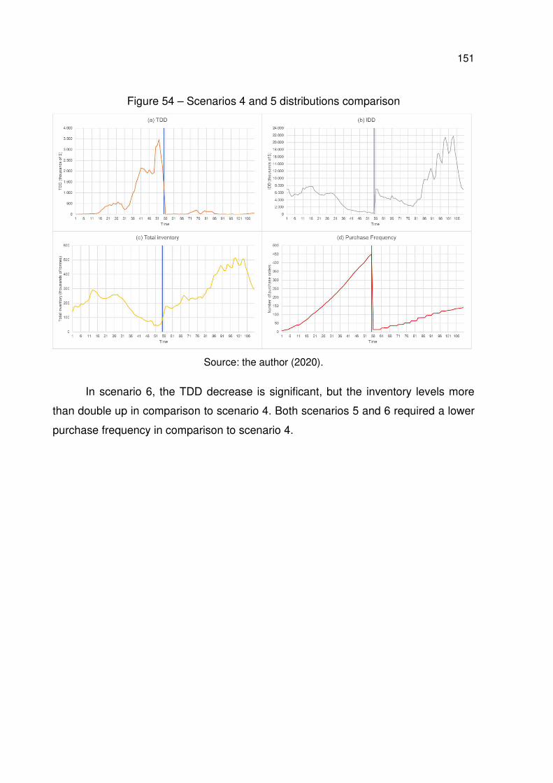
151
Figure 54 – Scenarios 4 and 5 distributions comparison
Source: the author (2020).
In scenario 6, the TDD decrease is significant, but the inventory levels more
than double up in comparison to scenario 4. Both scenarios 5 and 6 required a lower
purchase frequency in comparison to scenario 4.
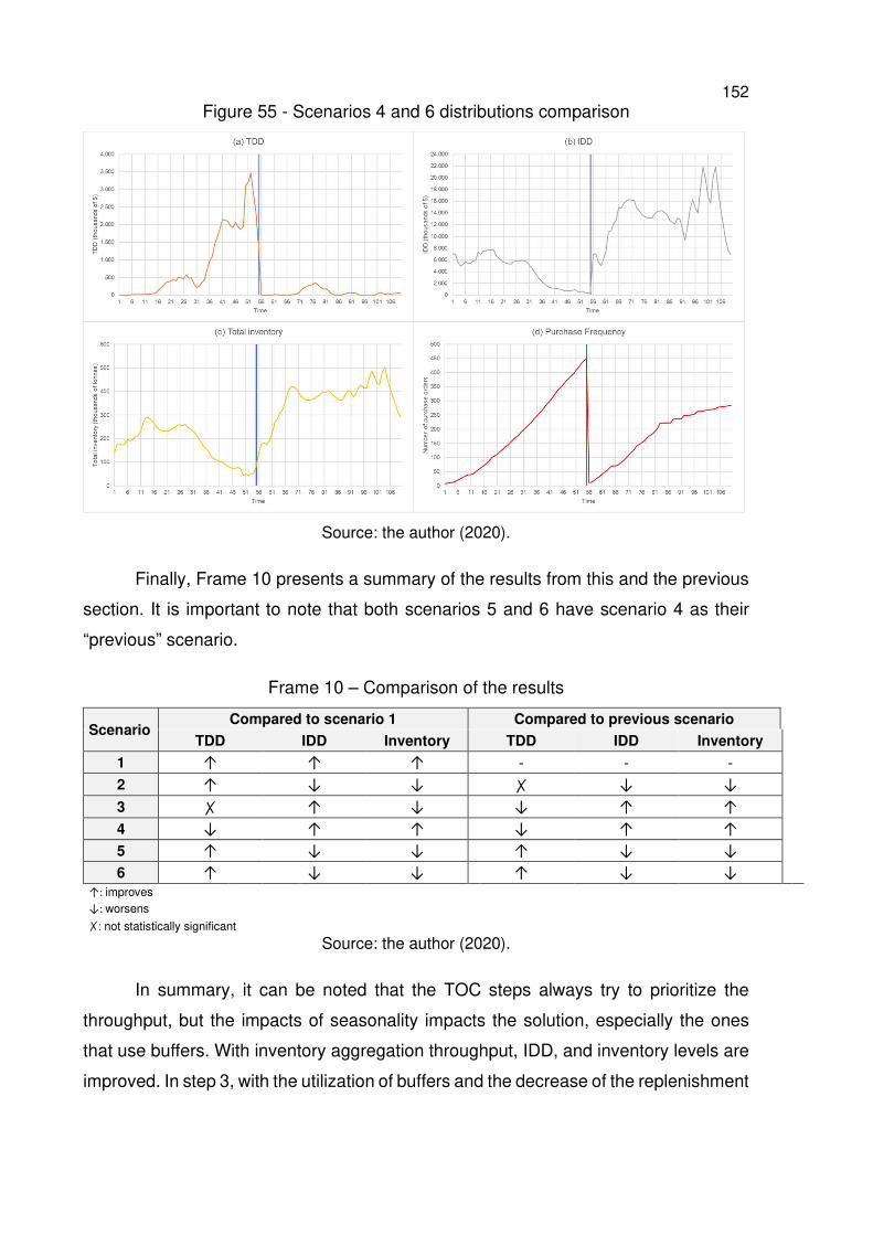
152 Figure 55 - Scenarios 4 and 6 distributions comparison
Source: the author (2020).
Finally, Frame 10 presents a summary of the results from this and the previous
section. It is important to note that both scenarios 5 and 6 have scenario 4 as their
“previous” scenario.
Frame 10 – Comparison of the results
Scenario Compared to scenario 1 Compared to previous scenario
TDD IDD Inventory TDD IDD Inventory
1 ↑ ↑ ↑ - - -
2 ↑ ↓ ↓ ✗ ↓ ↓
3 ✗ ↑ ↓ ↓ ↑ ↑
4 ↓ ↑ ↑ ↓ ↑ ↑
5 ↑ ↓ ↓ ↑ ↓ ↓
6 ↑ ↓ ↓ ↑ ↓ ↓
↑: improves
↓: worsens
✗: not statistically significant
Source: the author (2020).
In summary, it can be noted that the TOC steps always try to prioritize the
throughput, but the impacts of seasonality impacts the solution, especially the ones
that use buffers. With inventory aggregation throughput, IDD, and inventory levels are
improved. In step 3, with the utilization of buffers and the decrease of the replenishment
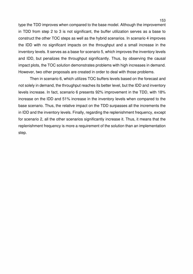
153 type the TDD improves when compared to the base model. Although the improvement
in TDD from step 2 to 3 is not significant, the buffer utilization serves as a base to
construct the other TOC steps as well as the hybrid scenarios. In scenario 4 improves
the IDD with no significant impacts on the throughput and a small increase in the
inventory levels. It serves as a base for scenario 5, which improves the inventory levels
and IDD, but penalizes the throughput significantly. Thus, by observing the causal
impact plots, the TOC solution demonstrates problems with high increases in demand.
However, two other proposals are created in order to deal with those problems.
Then in scenario 6, which utilizes TOC buffers levels based on the forecast and
not solely in demand, the throughput reaches its better level, but the IDD and inventory
levels increase. In fact, scenario 6 presents 92% improvement in the TDD, with 18%
increase on the IDD and 51% increase in the inventory levels when compared to the
base scenario. Thus, the relative impact on the TDD surpasses all the increments the
in IDD and the inventory levels. Finally, regarding the replenishment frequency, except
for scenario 2, all the other scenarios significantly increase it. Thus, it means that the
replenishment frequency is more a requirement of the solution than an implementation
step.
154 6 DISCUSSION OF THE RESULTS
This section aims to discuss the contributions of this research to the empirical
and academical aspects. Regarding the empirical impacts, a discussion of the impacts
to real case is conducted, clarifying the impacts for the company and its managers. In
the academic aspect, contributions aim to expand the Theory of Constraints literature
within the supply chain management context.
6.1 EMPIRICAL CONTRIBUTIONS WITHIN THE COMPANY CONTEXT
With long lead times, delays in replenishment, lost sales, and fierce competition
the studied case presented a huge opportunity for supply chain performance
improvement. As a big multinational company and with many foreign suppliers
composing its supply chain, those operational improvements can take time and often
are costly and risky. In that sense, simulation and modeling presents itself as a good
tool for more assertive, cheaper and safer decisions with regards to supply chain
redesign. Regarding the improvements necessary to elevate supply chain operations
the Theory of Constraints can offer a good guideline of practices and management
principles.
As detailed in the analysis of the results, better levels of throughput can and
must be achieved, directly and positively impacting the 30 million dollars of estimated
sales margin losses. At first, the implementation of the aggregated inventories at the
highest level of supply chain demonstrates an excellent increase in the throughput with
no statistically significant increases in the inventory levels. On the contrary, what is
perceived is a huge reduction of the inventories at the shop, in other words the
requesting units. If the throughput and the sales margin losses estimated by the
company could be related and directly connected, one could say that the 61% TDD
impact of the aggregation could represent a 18,3 million dollars improvement.
However, the connection between the throughput and sales margin loss is not part of
the scope of this research. Besides the high impact on the sales, a 61% decrease of
inventory in the 3 smaller plants is attractive as well for the business.
The utilization of buffers can also contribute to improve the results of the
company’s supply chain. The application of forecast-based buffers also show that
155 better results can be achieved through the application of TOC concepts, achieving up
to 92% improvement in the TDD. Drawing once again from the sales margin analogy,
the improvements found in this scenario would result in a 27,6 million dollars benefit,
directly impacting EBITDA. The sales margin loss would reduce to as low as 2,4 million
dollars. However, in order to achieve this impact an increase of inventories would be
necessary. Then, two valuable options derive from this research as suggestions of
impactful improvements for the company. One with significant impacts on the
throughput and no increase in the total inventory levels – but a significant decrease at
the lowest points of the supply chain – and other that maximizes the throughput and,
consequently, increases the inventories at the SC. A thoughtful comparison was
presented in this research, which can support manager’s decision for whichever path
is chosen, be it the maximum prioritization of the throughput, or a middle-term solution
that won’t impact the overall inventory level.
It is also important to mention that all TOC steps presented a significant impact
in at least one of the key variables. But it also presented some of the theory’s flaws,
especially when dealing with abrupt changes in demand. However, the solutions
presented in scenarios 6 and 7 demonstrate that the theory can be adapted and refined
to suit best the needs of the supply chains. Also, some limitations of the model have
to be considered, as the model do not aim to assess other supply chain related
impacts, such as logistics costs, manufacturing level components, production capacity,
storage limitations, etc.
Additionally, the model simulates only one part of the complete supply chain of
the organization. As previously stated, the state represents almost 30% of the total
supply chain. In that sense, other 70% remains as opportunities for the benefits here
described. Thus, the state could, for instance, serve as a pilot for the TOC
implementation in the company’s supply chain and be extended to the states as well.
Not only that, but the improvements and practices herein could be extended to the
international levels as well. In that sense, as Brazil represents 30% of the global
revenues of the company, there would be still other 70% in operations of other
countries that could benefits from the practices discussed. Demonstrating, huge
opportunities for improvement.
One final contribution regards the company’s data. The data structure of one of
the core and most important activities of the company is still very poorly managed. Lots
156 of manual work in conduct by both managers and analysts in order to have the raw-
material purchase requisitions and calculate the replenishment quantities. With a
yearly raw material spend that surpasses a billion dollars it is concerning to know that
there is no investment in software to support supply chain and planning decisions.
Additionally, it is odd that the company does not control the data of its own sales order.
As researched with the specialists there is no accurate and reliable method to have
historical data on sales delays and losses, for instance. This, however, is being studied
by the company in the implementation of a shared services center that will support
sales operations with improved data and track records. For the supply, planning and
replenishment tough, no initiative of such kind is planned. Thus, methods to improve
data analytics and technology for supply chain operations should be of the highest
importance.
6.2 ACADEMIC CONTRIBUTIONS
The research provides an empirical research of the Theory of Constraints within
the supply chain context. The causal impact analysis allows for a better understanding
of the TOC steps impacts and goals. It also demonstrates some problems especially
with regards to the buffer management proposals. It was noted that the buffers
performance are negatively impacted when sudden abrupt changes in demand occur,
just as claimed by Schragenheim (2010). The suggestion of turning TOC buffers ‘on’
and ‘off’ according to those expected changes was also tested. The solution –
presented in scenario 7 – affected positively the system’s throughput, but negatively
impacted the inventories and the IDD. Suggesting that Schragenheim’s (2010)
proposition might not be effective as expected. Nevertheless, drawing from the TOC
replenishment solution, a middle term approach is proposed in the research and the
positive effects of its application are demonstrated.
In a general sense, the research also aims to shed light into each one of the
TOC steps solutions that are directly linked to supply chain management. Other than
providing the causal impacts of the TOC implementation in a empirical supply chain,
some general findings regarding the objectives of each TOC solution step. It is
important to note though, that those findings might not apply to all cases, but might be
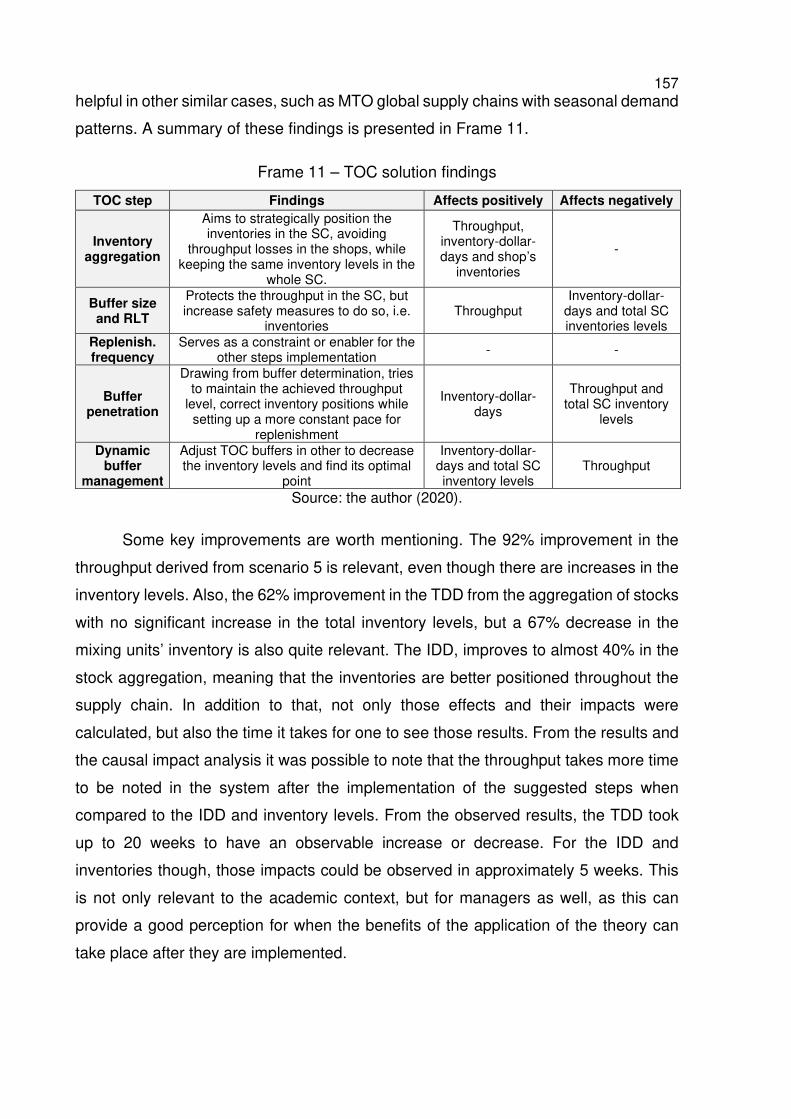
157 helpful in other similar cases, such as MTO global supply chains with seasonal demand
patterns. A summary of these findings is presented in Frame 11.
Frame 11 – TOC solution findings
TOC step Findings Affects positively Affects negatively
Inventory aggregation
Aims to strategically position the inventories in the SC, avoiding
throughput losses in the shops, while keeping the same inventory levels in the
whole SC.
Throughput, inventory-dollar-days and shop’s
inventories
-
Buffer size and RLT
Protects the throughput in the SC, but increase safety measures to do so, i.e.
inventories Throughput
Inventory-dollar-days and total SC inventories levels
Replenish. frequency
Serves as a constraint or enabler for the other steps implementation - -
Buffer penetration
Drawing from buffer determination, tries to maintain the achieved throughput
level, correct inventory positions while setting up a more constant pace for
replenishment
Inventory-dollar-days
Throughput and total SC inventory
levels
Dynamic buffer
management
Adjust TOC buffers in other to decrease the inventory levels and find its optimal
point
Inventory-dollar-days and total SC inventory levels
Throughput
Source: the author (2020).
Some key improvements are worth mentioning. The 92% improvement in the
throughput derived from scenario 5 is relevant, even though there are increases in the
inventory levels. Also, the 62% improvement in the TDD from the aggregation of stocks
with no significant increase in the total inventory levels, but a 67% decrease in the
mixing units’ inventory is also quite relevant. The IDD, improves to almost 40% in the
stock aggregation, meaning that the inventories are better positioned throughout the
supply chain. In addition to that, not only those effects and their impacts were
calculated, but also the time it takes for one to see those results. From the results and
the causal impact analysis it was possible to note that the throughput takes more time
to be noted in the system after the implementation of the suggested steps when
compared to the IDD and inventory levels. From the observed results, the TDD took
up to 20 weeks to have an observable increase or decrease. For the IDD and
inventories though, those impacts could be observed in approximately 5 weeks. This
is not only relevant to the academic context, but for managers as well, as this can
provide a good perception for when the benefits of the application of the theory can
take place after they are implemented.
158 An important point worth mentioning is regarding the increase of the
replenishment frequency, which can go up as 271% when the buffers are being used.
From the results and findings of this research, it seems that the replenishment
frequency acts more as a consequence, an enabler, or a constraint to the theory’s
implementation than a proper step to achieve determined benefits. It seems unlikely
that without the constant replenishment of the buffers, initiatives such as buffer
penetration and dynamic buffer management could occur. In that sense, it seems to
function like a reality check or a pre-requisite to move into those other initiatives.
Having concluded the discussions regarding the academic contributions of this
research, the next section presents the conclusion. Thus, a summary of the whole
research is demonstrated, pointing out its major contributions as well as future venues
of study.
159 7 CONCLUSION
Through this section, the research objectives are explored again and the
findings in relation to those are discussed. Additionally, some potential studies to
continue the research are suggested, as well as the limitations of the research and the
proposed model.
In the introduction, a contextualization of the current supply chain problems is
presented, while defining the research’s aim. The complexity of the global supply
chains and the fierce competition still pose as significant challenges to supply chain
management. Thus, supply chain redesign is a constant theme of discussion regarding
the operational improvement that can be achieved from it. The Theory of Constraints
presents itself as a solution for many of the problems faced by those supply chains.
Although not fully explored and somehow yet limited both academically and
empirically, the TOC proposes guidelines for supply chain management, especially
from the solution outlined and detailed by Schragenheim (2010). Deriving from the
theory’s inherent simplicity, the TOC supply chain solution aims to rely less on
forecasts, while being able to increase sales and reduce inventory levels. Although a
sound theory, not many studies detail the improvements achieved in supply chain by
the application of TOC supply chain solution. Therefore, observing this gap within the
literature this research proposes to asses each one of those steps and evaluate its
impacts.
In order to do so, a simulation study is proposed, based on an empirical case.
The case under study is the supply chain of an international company with operations
in Brazil. The company is active in more than 160 countries and is the segment market
leader in Brazil. Possessing 5 production units, 24 mixing units, the case of study focus
on the Rio Grande do Sul state – the most representative state for the company in the
country –, comprising of one production unit and three mixing units. Then, a system
dynamics model is proposed, by simulating the actual scenario of the company and
other scenarios that simulate the application of the TOC solution step by step. By this
procedural application of the steps an detailed understanding of its impacts and effects
are expected to be achieved.
Also, in order to sustain and create the knowledge background, a systematic
literature review was conducted. Within the SLR, 46 studies were analyzed completely
160 in order to create the basic theory’s foundation. Within this, a descriptive analysis of
the literature is presented, as well a content analysis exploring the TOC’s supply chain
solution and its performance measures.
Then the work methodology is streamlined. The data collection is conducted on
the field by the researcher with the support of relevant specialists, access to the
company’s database and its ERP system. In the data analysis, multivariate statistics
are used in order to test the significance of the results. Additionally, the causal impact
technique is utilized to measure TOC’s impact in the supply chain. The causal impact
provides good visuals resources to assess those impacts, as well as meaningful data
to support the negative and positive effects of the interventions on the system.
In the model construction, the base model is the initial step. After its verification
and validation, the model seems to be a good representation of the real-world scenario
and can be modified to assess the impacts of the TOC. Therefore, the creation of a
good simulation model is defined as a specific objective. With the validated model, it is
possible to simulate the TOC steps in the model. Also, TOC’s performance measures
are modelled in order to have the evaluation of its implementation. The model is
detailed in the model construction section, as well as each one of its modules. After
that the simulations are conducted and presented in the analysis of the results section.
The TOC steps are modeled, simulated and measured in comparison to the
base scenarios as well as with each previous step. From the causal impact analysis, it
is possible to note improvements in the system’s throughput of up to 92% and up to
62% decrease in inventories, depending on the scenario. The inventories at the shop
decrease up to 67% and the throughput results improve at the same time. Additionally,
two other scenarios are proposed in order to deal with the inherent seasonality found
in the system.
Although positive impacts are found, some negative effects are also discovered
and discussed. The difficulties to deal with high seasons of demand presented by the
buffer are analyzed and the TOC SC suggestion to deal with those is also tested.
However, as explained, the results are satisfactory and other scenarios tend to present
better results. Nevertheless, some insightful considerations, contributions and options
are made to the company that might help improve supply chain operations. Regarding
the academic aspect, a detailed empirical research is presented, and each TOC step
solution is detailed, as well as the outcomes and effects from that implementation.
161 Also, some limitations of the model must be considered. Since there is no actual
data for sales orders delays or missing sales due to those delays, the model uses the
raw-material consumption to calculate throughput losses. However, as a MTO
company, the raw material consumption can be defined as a good proxy for delayed
or lost sales orders. Also, the model does not consider logistics costs, other external
supply chain related issues, or the manufacturing level of operations. Thus, the last
step of the TOC solution, the virtual buffers and its prioritization, cannot be assessed.
For future venues of study, many scenarios can be suggested. Within the
company context, the of TOC’s application could be expanded to the whole country.
Also, the practical implementation of a pilot could be accompanied by a researcher to
test the results derived from this research. As an international company and supply
chain another subject that is rarely explored in the TOC context is the intercompany
trades and the complex dynamics involving the transfer prices. From the academic
perspective, the study could be replied in other similar scenarios – MTO, high level of
international suppliers, etc. – to refute or corroborate with the results derived from this
study. Moreover, any other empirical applications of TOC with quantitative measures
of its impacts are welcome and could be used for comparison and improvement of the
theory.
Overall, this research has presented some insightful concepts for the academic
and empirical contexts. It provided sound actions to improve the case’s supply chain
operations levels and options to support mangers decisions. In the academic context,
it explored a not yet fully scrutinized theme, that can be improved to gather more
adepts in the industry and more academic relevance.
162
REFERENCES
AGAMI, N.; SALEH, M.; RASMY, M. A hybrid dynamic framework for supply
chain performance improvement. IEEE Systems Journal, v. 6, n. 3, p. 469–478, 2012.
BASHIRI, M.; TABRIZI, M. M. Supply chain design: A holistic approach. Expert
Systems with Applications, v. 37, n. 1, p. 688–693, jan. 2010.
BELLANCA, L. Measuring interdisciplinary research: Analysis of co-authorship
for research staff at the University of York. Bioscience Horizons, v. 2, n. 2, p. 99–
112, 2009.
BERNARDI DE SOUZA, F.; PIRES, S. R. I. Theory of constraints contributions
to outbound logistics. Management Research Review, v. 33, n. 7, p. 683–700, 18 jun.
2010.
BERRY, D.; NAIM, M. M. Quantifying the relative improvements of redesign
strategies in a P.C. Supply chain. International Journal of Production Economics,
v. 46–47, p. 181–196, 1996.
BERTRAND, J. W. M.; FRANSOO, J. C. Operations management research
methodologies using quantitative modeling. [s.l: s.n.]. v. 22
BLACKSTONE, J. H. Theory of constraints - A status report. International
Journal of Production Research, v. 39, n. 6, p. 1053–1080, jan. 2001.
BRODERSEN, K. H. et al. Inferring causal impact using bayesian structural
time-series models. Annals of Applied Statistics, v. 9, n. 1, p. 247–274, 2015.
BUDD, C. S. Medidas Tradicionais em Finanças e Contabilidade, Problemas,
Revisões de Literatura e Medidas da TOC. In: COX III, J. F.; SCHLEIER, J. G. (Eds.).
. Handbook da Teoria das Restrições. Porto Alegre: Bookman, 2013. p. 345–382.
BUIL, R.; PIERA, M. A.; LASERNA, T. Operational and strategic supply model
redesign for an optical chain company using digital simulation. SIMULATION, v. 87, n.
8, p. 668–679, 9 ago. 2011.
CHALMERS, A. F. Deriving theories from the facts: induction. In: What is This
Thing Called Science? [s.l: s.n.].
CHANG, Y.-C.; CHANG, K.-H.; HUANG, C.-W. Integrate market demand
forecast and demand-pull replenishment to improve the inventory management
effectiveness of wafer fabrication. Proceedings of the Institution of Mechanical
Engineers, Part B: Journal of Engineering Manufacture, v. 228, n. 4, p. 617–636,
10 abr. 2014.
163
CHANG, Y.-C.; CHANG, K.-H.; SUN, W.-C. Enhancement of Inventory
Management for the Wafer Manufacturing Industry by Combining Market Demand
Forecast and Demand-Pull Replenishment. Journal of Testing and Evaluation, v.
43, n. 4, p. 948–963, jul. 2015.
CHANG, Y.-C. Y.-C.; CHANG, K.-H. K.-H.; LEI, Y.-C. Probe of the
Replenishment Strategy and Grouping Rule in the Semiconductor Industry. Journal
of Testing and Evaluation, v. 42, n. 2, p. 484–497, mar. 2014.
COBO, M. J. et al. Science mapping software tools: Review, analysis, and
cooperative study among tools. Journal of the American Society for Information
Science and Technology, v. 62, n. 7, p. 1382–1402, jul. 2011.
COLWYN JONES, T.; DUGDALE, D. Theory of Constraints: Transforming
Ideas? The British Accounting Review, v. 30, n. 1, p. 73–91, 1998.
COSTAS, J. J. J. et al. Applying Goldratt’s Theory of Constraints to reduce the
Bullwhip Effect through agent-based modeling. Expert Systems with Applications,
v. 42, n. 4, p. 2049–2060, mar. 2015.
DRESCH, A.; LACERDA, D. P.; ANTUNES, J. A. V. An Overflight Over
Research. In: Design Science Research. Cham: Springer International Publishing,
2015. p. 11–45.
DRESCH, A.; LACERDA, D. P.; ANTUNES JR., J. A. V. Design Science
Research. Cham: Springer International Publishing, 2015.
ER, M.; MACCARTHY, B. Managing product variety in multinational corporation
supply chains: A simulation study. Journal of Manufacturing Technology
Management, v. 17, n. 8, p. 1117–1138, 2006.
FILHO, T. A. R. et al. A new approach for decision making in distribution supply
chains: a theory of constraints perspective. International Journal of Logistics
Systems and Management, v. 25, n. 2, p. 266–282, 2016.
FU-REN LIN; YU-HUA PAI. Using multi-agent simulation and learning to design
new business processes. IEEE Transactions on Systems, Man, and Cybernetics -
Part A: Systems and Humans, v. 30, n. 3, p. 380–384, maio 2000.
GATES, D.; MAYOR, T.; GAMPENRIEDER, E. L. Global Manufacturing
OutlookKPMG International Cooperative. [s.l: s.n.]. Disponível em:
<https://assets.kpmg/content/dam/kpmg/pdf/2016/05/global-manufacturing-outlook-
competing-for-growth.pdf>.
GEODIS. Supply Chain Worldwide Survey. [s.l: s.n.]. Disponível em:
164
<https://geodis.com/sites/default/files/2019-03/170509_GEODIS_WHITE-
PAPER.PDF>. Acesso em: 25 fev. 2020.
GOLDRATT, E. M. Computerized shop floor schedulingInternational
Journal of Production Research, 1988.
GOLDRATT, E. M. It’s Not Luck. 1. ed. Great Barrington: The North River
Press, 1994.
GOLDRATT, E. M. Critical Chain. America, v. 8, p. 246, 1997.
GOLDRATT, E. M. Isn’t It Obvious? Great Barrington, MA: The North River
Press, 2009.
GOLDRATT, E. M.; COX, J. The Goal: A Process of Ongoing Improvement.
3rd Revise ed. Great Barrington, MA: The North River Press Publishing, 2004.
GOLDRATT, E. M.; SCHRAGENHEIM, E.; PTAK, C. A. Necessary but Not
Sufficient. Croton-on-Hudson: NY: North River Press, 2000.
GUPTA, M. Constraints management--recent advances and practices.
International Journal of Production Research, v. 41, n. 4, p. 647–659, 14 jan. 2003.
GUPTA, M.; ANDERSEN, S. Revisiting local TOC measures in an internal
supply chain: A note. International Journal of Production Research, v. 50, n. 19, p.
5363–5371, out. 2012.
GUPTA, M.; ANDERSEN, S. Throughput/inventory dollar-days: TOC-based
measures for supply chain collaboration. International Journal of Production
Research, v. 56, n. 13, p. 4659–4675, 3 jul. 2018.
GUPTA, M. C.; BOYD, L. H. Theory of constraints: A theory for operations
management. International Journal of Operations and Production Management,
v. 28, n. 10, p. 991–1012, 2008.
GUPTA, M.; KO, H.-J.; MIN, H. TOC-based performance measures and five
focusing steps in a job-shop manufacturing environment. International Journal of
Production Research, v. 40, n. 4, p. 907–930, 14 jan. 2002.
GUPTA, M.; SNYDER, D. Comparing TOC with MRP and JIT: a literature
review. International Journal of Production Research, v. 47, n. 13, p. 3705–3739,
11 jul. 2009.
HOCHBERG, Y. A sharper bonferroni procedure for multiple tests of
significance. Biometrika, 1988.
HUNT, K. L. et al. Using V-A-T analysis as a framework for supply chain
management: A case study. European Journal of Economics, Finance and
165
Administrative Sciences, n. 17, p. 69–80, mar. 2009.
IKEZIRI, L. M. et al. Theory of constraints: review and bibliometric analysis.
International Journal of Production Research, v. 57, n. 15–16, p. 5068–5102, 2019.
JAIN, J. et al. Supply Chain Management: Literature Review and Some Issues.
Journal of Studies on Manufacturing, v. 1, n. 1, p. 11–25, 6 ago. 2010.
JI, S. W.; LI, C. C.; CHEN, J. J. Study on Manufacturing Engineering with Supply
Chain Profit Model of Fast Moving Consumer Goods Based on TOC Operation Mode.
Applied Mechanics and Materials, v. 345, p. 473–476, ago. 2013.
JIANG, X.-Y.; WU, H.-H. Optimization of setup frequency for TOC supply chain
replenishment system with capacity constraints. Neural Computing and
Applications, v. 23, n. 6, p. 1831–1838, 2013a.
JIANG, X.-Y. X.-Y.; WU, H.-H. H.-H. Optimization of Setup Frequency for TOC
Supply Chain Replenishment Systems Based on Pareto Particle Swarm Optimization.
Journal of Networks, v. 8, n. 12, p. 2964–2971, 10 dez. 2013b.
JIANG, X. et al. Diverse replenishment frequency model for TOC supply chain
replenishment systems with capacity constraints. International Journal of Modelling,
Identification and Control, v. 19, n. 3, p. 248–256, 2013.
JOEL HAVEMANN. The Financial Crisis of 2008 | Britannica.com. Disponível
em: <https://www.britannica.com/topic/Financial-Crisis-of-2008-The-1484264>.
Acesso em: 5 mar. 2019.
K. J. YOUNGMAN. Theory of Constraints Supply Chain Replenishment.
Disponível em: <http://www.dbrmfg.co.nz/Supply Chain Replenishment.htm>. Acesso
em: 16 fev. 2020.
KAIHARA, T. Supply chain management with market economics. International
Journal of Production Economics, v. 73, n. 1, p. 5–14, 31 ago. 2001.
KAIJUN, L.; WANG YUXIA, W. X. Research on inventory control policies for
nonstationary demand based on TOC. International Journal of Computational
Intelligence Systems, v. 3, n. May 2015, p. 114–128, dez. 2010.
KARAGIANNAKI, A.; DOUKIDIS, G.; PRAMATARI, K. A framework for mapping
the RFID-enabled process redesign in a simulation model. Journal of the Operational
Research Society, v. 65, n. 11, p. 1700–1710, nov. 2014.
KIM, S.; MABIN, V. J.; DAVIES, J. The theory of constraints thinking processes:
retrospect and prospect. International Journal of Operations & Production
Management, v. 28, n. 2, p. 155–184, 2008.
166
LAW, A. M. Simulation Modeling and Analysis. 5. ed. [s.l: s.n.].
LENG, K.; CHEN, X. A genetic algorithm approach for TOC-based supply chain
coordination. Applied Mathematics and Information Sciences, v. 6, n. 3, p. 767–
774, 2012.
LEWIS-BECK, M.; BRYMAN, A.; FUTING LIAO, T. The SAGE Encyclopedia
of Social Science Research MethodsThousand Oaks, California, 2004. Disponível
em: <https://methods.sagepub.com/reference/the-sage-encyclopedia-of-social-
science-research-methods>
MABIN, V. J.; BALDERSTONE, S. J. The performance of the theory of
constraints methodology. International Journal of Operations & Production
Management, v. 23, n. 6, p. 568–595, jun. 2003.
MABIN, V. J.; DAVIES, J. The TOC Thinking Processes - Their Nature and Use
Reflections and Consolidation. In: COX, J. F.; JOHN G. SCHLEIER (Eds.). . Theory
of Constraints Handbook. [s.l.] McGraw-Hill, 2010. p. 631–669.
MARGARETHA; BUDIASTUTI, D.; SAHRONI, T. R. Application of theory of
constraint supply chain replenishment system in fast moving consumer goods
company. International Journal of Supply Chain Management, v. 6, n. 4, p. 167–
175, 2017.
MARTINS, S. et al. An optimization-simulation approach to the network redesign
problem of pharmaceutical wholesalers. Computers & Industrial Engineering, v.
106, p. 315–328, abr. 2017.
MENTZER, J. T.; FLINT, D. J. Validity in logistics research. Journal of
Business Logistics, 1997.
MERIGÓ, J. M.; YANG, J. B. A bibliometric analysis of operations research and
management science. Omega (United Kingdom), v. 73, p. 37–48, 2017.
MISHRA, N. et al. A CBFSA approach to resolve the distributed manufacturing
process planning problem in a supply chain environment. International Journal of
Production Research, v. 50, n. 2, p. 535–550, 15 jan. 2012.
MITROFF, I. I. et al. On Managing Science in the Systems Age: Two Schemas
for the Study of Science as a Whole Systems Phenomenon. Interfaces, v. 4, n. 3, p.
46–58, 1974.
MIZARRO, S. Relevance: The whole history. Journal of the American Society
for Information Science, v. 48, n. 9, p. 810–832, 1997.
MODI, K.; LOWALEKAR, H.; BHATTA, N. M. K. Revolutionizing supply chain
167
management the theory of constraints way: a case studyInternational Journal of
Production Research, 2018. Disponível em:
<https://www.scopus.com/inward/record.uri?eid=2-s2.0-
85053898181&doi=10.1080%2F00207543.2018.1523579&partnerID=40&md5=e017
e30fa92d0968eda1329ff9c5fc37>
MORANDI, M. I. W. M.; CAMARGO, L. F. R. Systematic Literature Review. In:
Design Science Research. [s.l.] Springer International Publishing, 2015. p. 129–158.
NAIM, M. M.; DISNEY, S. M.; EVANS, G. N. Minimum Reasonable Inventory
and the Bullwhip Effect in an Automotive Enterprise; A “Foresight Vehicle”
Demonstrator. SAE Technical Papers. Anais...4 mar. 2002Disponível em:
<https://www.scopus.com/inward/record.uri?eid=2-s2.0-
84877555370&doi=10.4271%2F2002-01-
0461&partnerID=40&md5=0bda7f593f1952b0a40e9b725358f3f8>
NAOR, M.; BERNARDES, E. S.; COMAN, A. Theory of constraints: Is it a theory
and a good one? International Journal of Production Research, v. 51, n. 2, p. 542–
554, 2013.
NOREEN, E.; SMITH, D.; MACKEY, J. T. A Teoria das Restrições e Suas
Implicações na Contabilidade Gerencial. São Paulo: Educator, 1996.
PARSAEI, Z.; NAHAVANDI, N.; ELMEKKAWY, T. Buffer size determination for
drum-buffer-rope controlled supply chain networks. International Journal of Agile
Systems and Management, v. 5, n. 2, p. 151–163, 2012.
PÉREZ, J. Toc for world class global supply chain management. Computers &
Industrial Engineering, v. 33, n. 1–2, p. 289–293, out. 1997.
PETERS, H. P. F.; VAN RAAN, A. F. J. Structuring scientific activities by co-
author analysis. Scientometrics, v. 20, n. 1, p. 235–255, jan. 1991.
PIDD, M. Tools for thinking: modelling in management science. 2nd. ed.
Chichester: John Wiley & Sons Ltd, 2003.
PIRARD, F.; IASSINOVSKI, S.; RIANE, F. A generic scalable simulation model
for strategic supply chain management with emphasis on production activities.
International Journal of Computer Integrated Manufacturing, v. 21, n. 4, p. 455–
467, 2008.
PONTE, B. et al. Holism versus reductionism in supply chain management: An
economic analysis. Decision Support Systems, v. 86, p. 83–94, jun. 2016.
PUCHE, J. et al. Systemic approach to supply chain management through the
168
viable system model and the theory of constraints. Production Planning and Control,
v. 27, n. 5, p. 421–430, 3 abr. 2016.
RAHMAN, S. Theory of constraints: A review of the philosophy and its
applications. International Journal of Operations & Production Management, v.
18, n. 4, p. 336–355, 1998.
SAUNDERS, M.; LEWIS, P.; THORNHILL, A. Understanding research
philosophies and approaches. In: Research Methods for Business Students. 6th.
ed. Harlow: Pearson Education, 2012a. p. 126–157.
SAUNDERS, M.; LEWIS, P.; THORNHILL, A. Research Methods for
Business Students. 6th. ed. Harlow: Pearson Education, 2012b.
SCHEINKOPF, L. J. Thinking Processes Including S&T Trees. In: COX, J. F.;
SCHLEIER, J. G. (Eds.). . Theory of Constraints Handbook. [s.l.] McGraw-Hill, 2010.
p. 729–786.
SCHRAGENHEIM, A. Supply Chain Management. In: COX, J. F.; SCHLEIER,
J. G. (Eds.). . Theory of Constraints Handbook. [s.l.] McGraw-Hill, 2010. p. 265–
301.
SCHRAGENHEIM, E.; DETTMER, H.; PATTERSON, J. Supply Chain
Management at Warp Speed. 2009.
SEURING, S.; GOLD, S. Conducting content-analysis based literature reviews
in supply chain management. Supply Chain Management, v. 17, n. 5, p. 544–555,
2012.
SHAPIRO, S. S.; WILK, M. B. An Analysis of Variance Test for Normality
(Complete Samples). Biometrika, 1965.
SIMATUPANG, T. M.; WRIGHT, A. C.; SRIDHARAN, R. Applying the theory of
constraints to supply chain collaboration. Supply Chain Management: An
International Journal, v. 9, n. 1, p. 57–70, 2004.
SLACK, N.; LEWIS, M.; BATES, H. The two worlds of operations management
research and practice. International Journal of Operations & Production
Management, v. 24, n. 4, p. 372–387, 2004.
SMITH, C.; PTAK, C. Integrated Supply Chain: Beyond MRP — How Actively
Synchronized Replenishment (ASR) Will Meet the Current Materials Synchronization
Challenge. In: COX, J. F.; SCHLEIER, J. G. (Eds.). . Theory of Constraints
Handbook. [s.l.] McGraw-Hill, 2010. p. 303–332.
SPENCER, M. S.; COX, J. F. Optimum production technology (OPT) and the
169
theory of constraints (TOC): Analysis and genealogy. International Journal of
Production Research, v. 33, n. 6, p. 1495–1504, 1995.
STERMAN, J. D. Business dynamics: Systems thinking and modeling for
a complex world. [s.l: s.n.].
STEVENS, G. C.; JOHNSON, M. Integrating the Supply Chain … 25 years on.
International Journal of Physical Distribution and Logistics Management, v. 46,
n. 1, p. 19–42, 2016.
SUN, R. et al. Inventory Control Policy for E-tail Organizations Based on TOC.
Information Technology Journal, v. 12, n. 24, p. 8171–8175, 1 dez. 2013.
TELLES, E. S. et al. Drum-buffer-rope in an engineering-to-order system: An
analysis of an aerospace manufacturer using data envelopment analysis (DEA).
International Journal of Production Economics, n. September, 2019.
Timeline: The unfolding eurozone crisis - BBC News. Disponível em:
<https://www.bbc.com/news/business-13856580>. Acesso em: 5 mar. 2019.
TOWILL, D. R. System dynamics— background, methodology, and
applications: Part 1: Background and methodology. Computing and Control
Engineering Journal, v. 4, n. 5, p. 201–208, 1993a.
TOWILL, D. R. System dynamics—background, methodology, and applications.
Part 2: Applications. Computing & Control Engineering Journal, v. 4, n. 6, p. 201–
208, 1993b.
TOWILL, D. R. System dynamics—background, methodology, and applications.
Part 1: Background and methodology. Computing & Control Engineering Journal,
v. 4, n. 5, p. 201–208, 1993c.
TSOU, C.-M. C.-M. On the strategy of supply chain collaboration based on
dynamic inventory target level management: A theory of constraint perspective.
Applied Mathematical Modelling, v. 37, n. 7, p. 5204–5214, abr. 2013.
TULASI, C. L.; RAO, A. R. Review on theory of constraints. International
Journal of Advances in Engineering & Technology, v. 3, n. 1, p. 334–344, 2012.
VAN ECK, N. J.; WALTMAN, L. Software survey: VOSviewer, a computer
program for bibliometric mapping. Scientometrics, v. 84, n. 2, p. 523–538, 31 ago.
2010.
WALKER, W. T. Practical application of drum-buffer-rope to synchronize a two-
stage supply chain. Production and Inventory Management Journal, v. 43, n. 3/4,
p. 13–23, 2002.
170
WATSON, K. J.; BLACKSTONE, J. H.; GARDINER, S. C. The evolution of a
management philosophy: The theory of constraints. Journal of Operations
Management, v. 25, n. 2, p. 387–402, 2007.
WATSON, K.; POLITO, T. Comparison of DRP and TOC financial performance
within a multi-product, multi-echelon physical distribution environment. International
Journal of Production Research, v. 41, n. 4, p. 741–765, 2003.
WORLD BANK GROUP. Agriculture, forestry, and fishing, value added (%
of GDP) - Brazil | Data. Disponível em:
<https://data.worldbank.org/indicator/NV.AGR.TOTL.ZS?locations=BR>. Acesso em:
7 nov. 2019.
WU, H.-H. et al. A study of an enhanced simulation model for TOC supply chain
replenishment system under capacity constraint. Expert Systems with Applications,
v. 37, n. 9, p. 6435–6440, set. 2010.
WU, H.-H. et al. A study of the elongated replenishment frequency of TOC
supply chain replenishment systems in plants. International Journal of Production
Research, v. 50, n. 19, p. 5567–5581, out. 2012.
WU, H.-H.; LEE, A. H. I.; TSAI, T.-P. P. A two-level replenishment frequency
model for TOC supply chain replenishment systems under capacity constraint.
Computers and Industrial Engineering, v. 72, p. 152–159, jun. 2014.
YUAN, K.-J.; CHANG, S.-H.; LI, R.-K. Enhancement of Theory of Constraints
replenishment using a novel generic buffer management procedure. International
Journal of Production Research, v. 41, n. 4, p. 725–740, 14 jan. 2003.
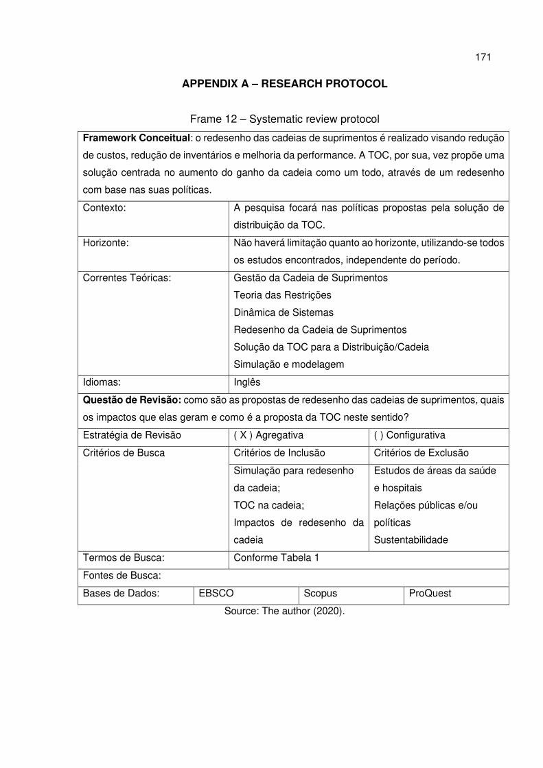
171
APPENDIX A – RESEARCH PROTOCOL
Frame 12 – Systematic review protocol
Framework Conceitual: o redesenho das cadeias de suprimentos é realizado visando redução
de custos, redução de inventários e melhoria da performance. A TOC, por sua, vez propõe uma
solução centrada no aumento do ganho da cadeia como um todo, através de um redesenho
com base nas suas políticas.
Contexto: A pesquisa focará nas políticas propostas pela solução de
distribuição da TOC.
Horizonte: Não haverá limitação quanto ao horizonte, utilizando-se todos
os estudos encontrados, independente do período.
Correntes Teóricas: Gestão da Cadeia de Suprimentos
Teoria das Restrições
Dinâmica de Sistemas
Redesenho da Cadeia de Suprimentos
Solução da TOC para a Distribuição/Cadeia
Simulação e modelagem
Idiomas: Inglês
Questão de Revisão: como são as propostas de redesenho das cadeias de suprimentos, quais
os impactos que elas geram e como é a proposta da TOC neste sentido?
Estratégia de Revisão ( X ) Agregativa ( ) Configurativa
Critérios de Busca Critérios de Inclusão Critérios de Exclusão
Simulação para redesenho
da cadeia;
TOC na cadeia;
Impactos de redesenho da
cadeia
Estudos de áreas da saúde
e hospitais
Relações públicas e/ou
políticas
Sustentabilidade
Termos de Busca: Conforme Tabela 1
Fontes de Busca:
Bases de Dados: EBSCO Scopus ProQuest
Source: The author (2020).
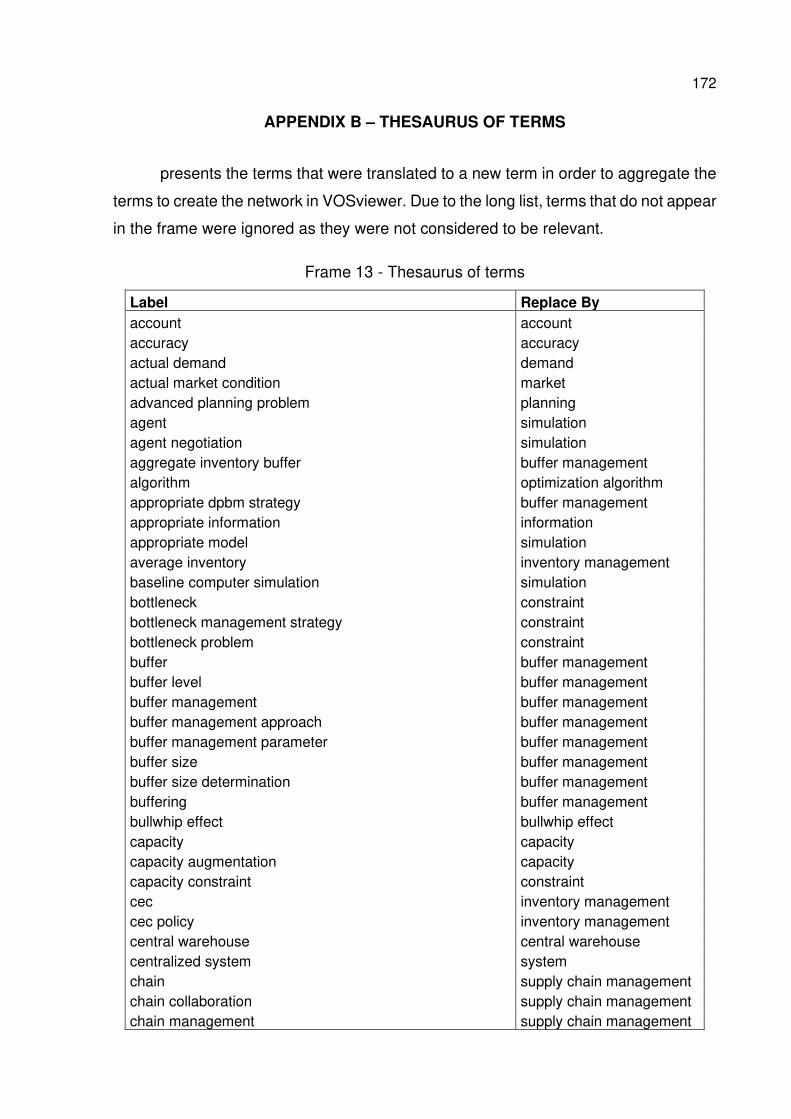
172
APPENDIX B – THESAURUS OF TERMS
presents the terms that were translated to a new term in order to aggregate the
terms to create the network in VOSviewer. Due to the long list, terms that do not appear
in the frame were ignored as they were not considered to be relevant.
Frame 13 - Thesaurus of terms
Label Replace By
account account accuracy accuracy actual demand demand actual market condition market advanced planning problem planning agent simulation agent negotiation simulation aggregate inventory buffer buffer management algorithm optimization algorithm appropriate dpbm strategy buffer management appropriate information information appropriate model simulation average inventory inventory management baseline computer simulation simulation bottleneck constraint bottleneck management strategy constraint bottleneck problem constraint buffer buffer management buffer level buffer management buffer management buffer management buffer management approach buffer management buffer management parameter buffer management buffer size buffer management buffer size determination buffer management buffering buffer management bullwhip effect bullwhip effect capacity capacity capacity augmentation capacity capacity constraint constraint cec inventory management cec policy inventory management central warehouse central warehouse centralized system system chain supply chain management chain collaboration supply chain management chain management supply chain management
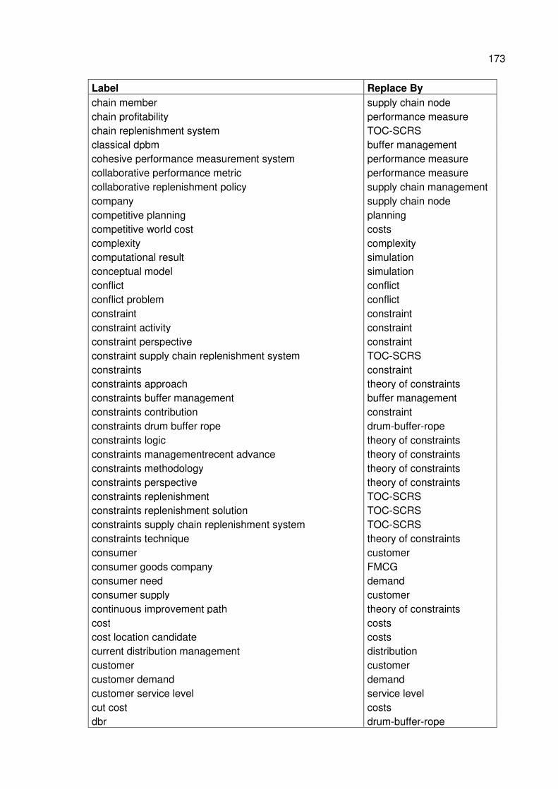
173
Label Replace By
chain member supply chain node chain profitability performance measure chain replenishment system TOC-SCRS classical dpbm buffer management cohesive performance measurement system performance measure collaborative performance metric performance measure collaborative replenishment policy supply chain management company supply chain node competitive planning planning competitive world cost costs complexity complexity computational result simulation conceptual model simulation conflict conflict conflict problem conflict constraint constraint constraint activity constraint constraint perspective constraint constraint supply chain replenishment system TOC-SCRS constraints constraint constraints approach theory of constraints constraints buffer management buffer management constraints contribution constraint constraints drum buffer rope drum-buffer-rope constraints logic theory of constraints constraints managementrecent advance theory of constraints constraints methodology theory of constraints constraints perspective theory of constraints constraints replenishment TOC-SCRS constraints replenishment solution TOC-SCRS constraints supply chain replenishment system TOC-SCRS constraints technique theory of constraints consumer customer consumer goods company FMCG consumer need demand consumer supply customer continuous improvement path theory of constraints cost costs cost location candidate costs current distribution management distribution customer customer customer demand demand customer service level service level cut cost costs dbr drum-buffer-rope
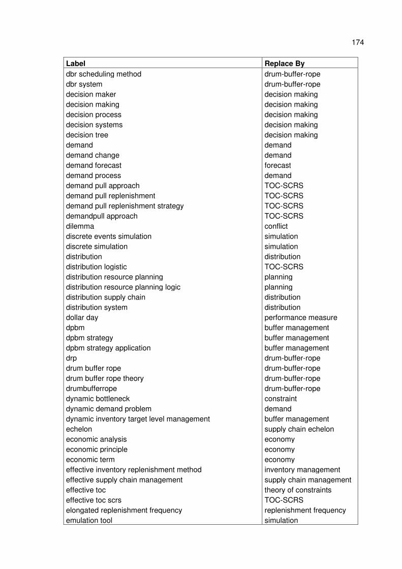
174
Label Replace By
dbr scheduling method drum-buffer-rope dbr system drum-buffer-rope decision maker decision making decision making decision making decision process decision making decision systems decision making decision tree decision making demand demand demand change demand demand forecast forecast demand process demand demand pull approach TOC-SCRS demand pull replenishment TOC-SCRS demand pull replenishment strategy TOC-SCRS demandpull approach TOC-SCRS dilemma conflict discrete events simulation simulation discrete simulation simulation distribution distribution distribution logistic TOC-SCRS distribution resource planning planning distribution resource planning logic planning distribution supply chain distribution distribution system distribution dollar day performance measure dpbm buffer management dpbm strategy buffer management dpbm strategy application buffer management drp drum-buffer-rope drum buffer rope drum-buffer-rope drum buffer rope theory drum-buffer-rope drumbufferrope drum-buffer-rope dynamic bottleneck constraint dynamic demand problem demand dynamic inventory target level management buffer management echelon supply chain echelon economic analysis economy economic principle economy economic term economy effective inventory replenishment method inventory management effective supply chain management supply chain management effective toc theory of constraints effective toc scrs TOC-SCRS elongated replenishment frequency replenishment frequency emulation tool simulation
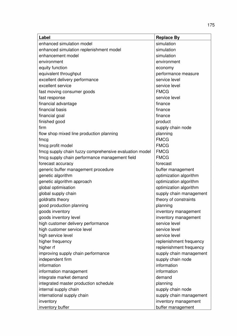
175
Label Replace By
enhanced simulation model simulation enhanced simulation replenishment model simulation enhancement model simulation environment environment equity function economy equivalent throughput performance measure excellent delivery performance service level excellent service service level fast moving consumer goods FMCG fast response service level financial advantage finance financial basis finance financial goal finance finished good product firm supply chain node flow shop mixed line production planning planning fmcg FMCG fmcg profit model FMCG fmcg supply chain fuzzy comprehensive evaluation model FMCG fmcg supply chain performance management field FMCG forecast accuracy forecast generic buffer management procedure buffer management genetic algorithm optimization algorithm genetic algorithm approach optimization algorithm global optimisation optimization algorithm global supply chain supply chain management goldratts theory theory of constraints good production planning planning goods inventory inventory management goods inventory level inventory management high customer delivery performance service level high customer service level service level high service level service level higher frequency replenishment frequency higher rf replenishment frequency improving supply chain performance supply chain management independent firm supply chain node information information information management information integrate market demand demand integrated master production schedule planning internal supply chain supply chain node international supply chain supply chain management inventory inventory management inventory buffer buffer management
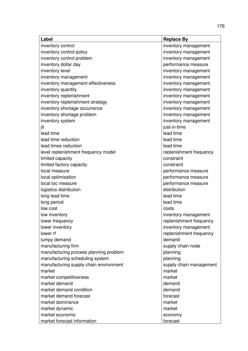
176
Label Replace By
inventory control inventory management inventory control policy inventory management inventory control problem inventory management inventory dollar day performance measure inventory level inventory management inventory management inventory management inventory management effectiveness inventory management inventory quantity inventory management inventory replenishment inventory management inventory replenishment strategy inventory management inventory shortage occurrence inventory management inventory shortage problem inventory management inventory system inventory management jit just-in-time lead time lead time lead time reduction lead time lead times reduction lead time level replenishment frequency model replenishment frequency limited capacity constraint limited factory capacity constraint local measure performance measure local optimisation performance measure local toc measure performance measure logistics distribution distribution long lead time lead time long period lead time low cost costs low inventory inventory management lower frequency replenishment frequency lower inventory inventory management lower rf replenishment frequency lumpy demand demand manufacturing firm supply chain node manufacturing process planning problem planning manufacturing scheduling system planning manufacturing supply chain environment supply chain management market market market competitiveness market market demand demand market demand condition demand market demand forecast forecast market dominance market market dynamic market market economic economy market forecast information forecast
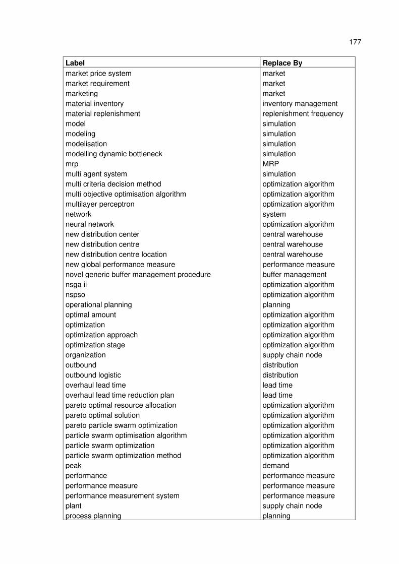
177
Label Replace By
market price system market market requirement market marketing market material inventory inventory management material replenishment replenishment frequency model simulation modeling simulation modelisation simulation modelling dynamic bottleneck simulation mrp MRP multi agent system simulation multi criteria decision method optimization algorithm multi objective optimisation algorithm optimization algorithm multilayer perceptron optimization algorithm network system neural network optimization algorithm new distribution center central warehouse new distribution centre central warehouse new distribution centre location central warehouse new global performance measure performance measure novel generic buffer management procedure buffer management nsga ii optimization algorithm nspso optimization algorithm operational planning planning optimal amount optimization algorithm optimization optimization algorithm optimization approach optimization algorithm optimization stage optimization algorithm organization supply chain node outbound distribution outbound logistic distribution overhaul lead time lead time overhaul lead time reduction plan lead time pareto optimal resource allocation optimization algorithm pareto optimal solution optimization algorithm pareto particle swarm optimization optimization algorithm particle swarm optimisation algorithm optimization algorithm particle swarm optimization optimization algorithm particle swarm optimization method optimization algorithm peak demand performance performance measure performance measure performance measure performance measurement system performance measure plant supply chain node process planning planning
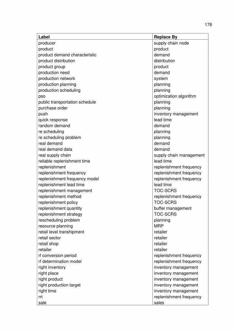
178
Label Replace By
producer supply chain node product product product demand characteristic demand product distribution distribution product group product production need demand production network system production planning planning production scheduling planning pso optimization algorithm public transportation schedule planning purchase order planning push inventory management quick response lead time random demand demand re scheduling planning re scheduling problem planning real demand demand real demand data demand real supply chain supply chain management reliable replenishment time lead time replenishment replenishment frequency replenishment frequency replenishment frequency replenishment frequency model replenishment frequency replenishment lead time lead time replenishment management TOC-SCRS replenishment method replenishment frequency replenishment policy TOC-SCRS replenishment quantity buffer management replenishment strategy TOC-SCRS rescheduling problem planning resource planning MRP retail level transhipment retailer retail sector retailer retail shop retailer retailer retailer rf conversion period replenishment frequency rf determination model replenishment frequency right inventory inventory management right place inventory management right product inventory management right production target inventory management right time inventory management rrt replenishment frequency sale sales
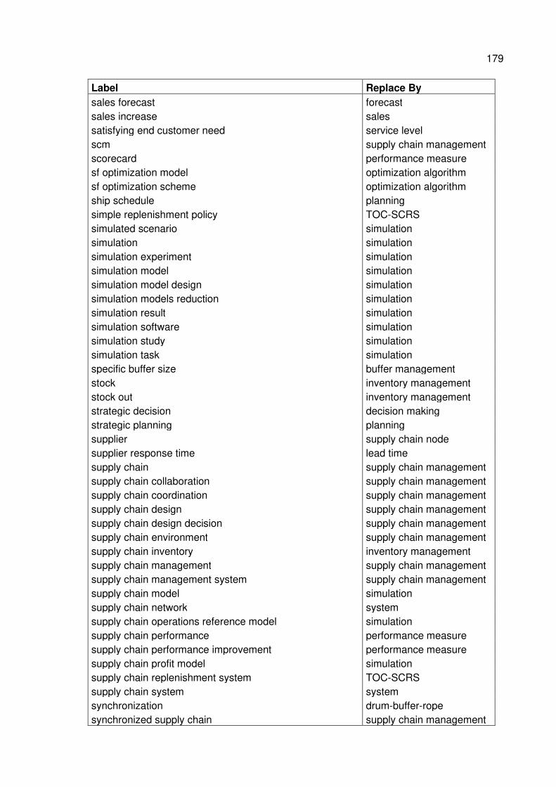
179
Label Replace By
sales forecast forecast sales increase sales satisfying end customer need service level scm supply chain management scorecard performance measure sf optimization model optimization algorithm sf optimization scheme optimization algorithm ship schedule planning simple replenishment policy TOC-SCRS simulated scenario simulation simulation simulation simulation experiment simulation simulation model simulation simulation model design simulation simulation models reduction simulation simulation result simulation simulation software simulation simulation study simulation simulation task simulation specific buffer size buffer management stock inventory management stock out inventory management strategic decision decision making strategic planning planning supplier supply chain node supplier response time lead time supply chain supply chain management supply chain collaboration supply chain management supply chain coordination supply chain management supply chain design supply chain management supply chain design decision supply chain management supply chain environment supply chain management supply chain inventory inventory management supply chain management supply chain management supply chain management system supply chain management supply chain model simulation supply chain network system supply chain operations reference model simulation supply chain performance performance measure supply chain performance improvement performance measure supply chain profit model simulation supply chain replenishment system TOC-SCRS supply chain system system synchronization drum-buffer-rope synchronized supply chain supply chain management
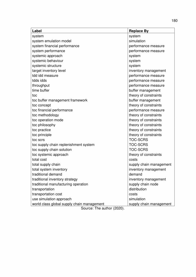
180
Label Replace By
system system system emulation model simulation system financial performance performance measure system performance performance measure systemic approach system systemic behaviour system systemic structure system target inventory level inventory management tdd idd measure performance measure tdds idds performance measure throughput performance measure time buffer buffer management toc theory of constraints toc buffer management framework buffer management toc concept theory of constraints toc financial performance performance measure toc methodology theory of constraints toc operation mode theory of constraints toc philosophy theory of constraints toc practice theory of constraints toc principle theory of constraints toc scrs TOC-SCRS toc supply chain replenishment system TOC-SCRS toc supply chain solution TOC-SCRS toc systemic approach theory of constraints total cost costs total supply chain supply chain management total system inventory inventory management traditional demand demand traditional inventory strategy inventory management traditional manufacturing operation supply chain node transportation distribution transportation cost costs use simulation approach simulation world class global supply chain management supply chain management
Source: The author (2020).
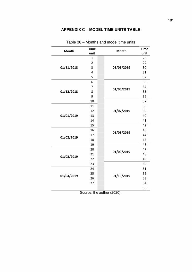
181
APPENDIX C – MODEL TIME UNITS TABLE
Table 30 – Months and model time units
Month Time
unit Month
Time
unit
01/11/2018
1
01/05/2019
28
2 29
3 30
4 31
5 32
01/12/2018
6
01/06/2019
33
7 34
8 35
9 36
10
01/07/2019
37
01/01/2019
11 38
12 39
13 40
14 41
15
01/08/2019
42
01/02/2019
16 43
17 44
18 45
19
01/09/2019
46
01/03/2019
20 47
21 48
22 49
23
01/10/2019
50
01/04/2019
24 51
25 52
26 53
27 54
55
Source: the author (2020).
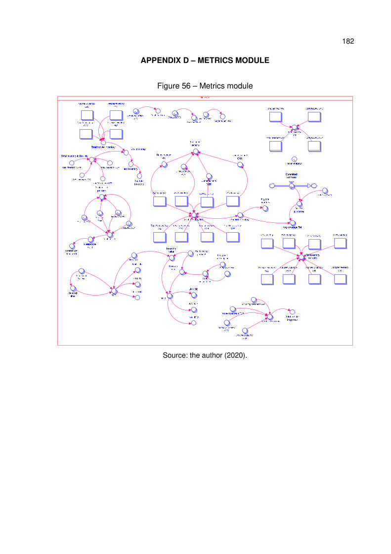
182
APPENDIX D – METRICS MODULE
Figure 56 – Metrics module
Source: the author (2020).
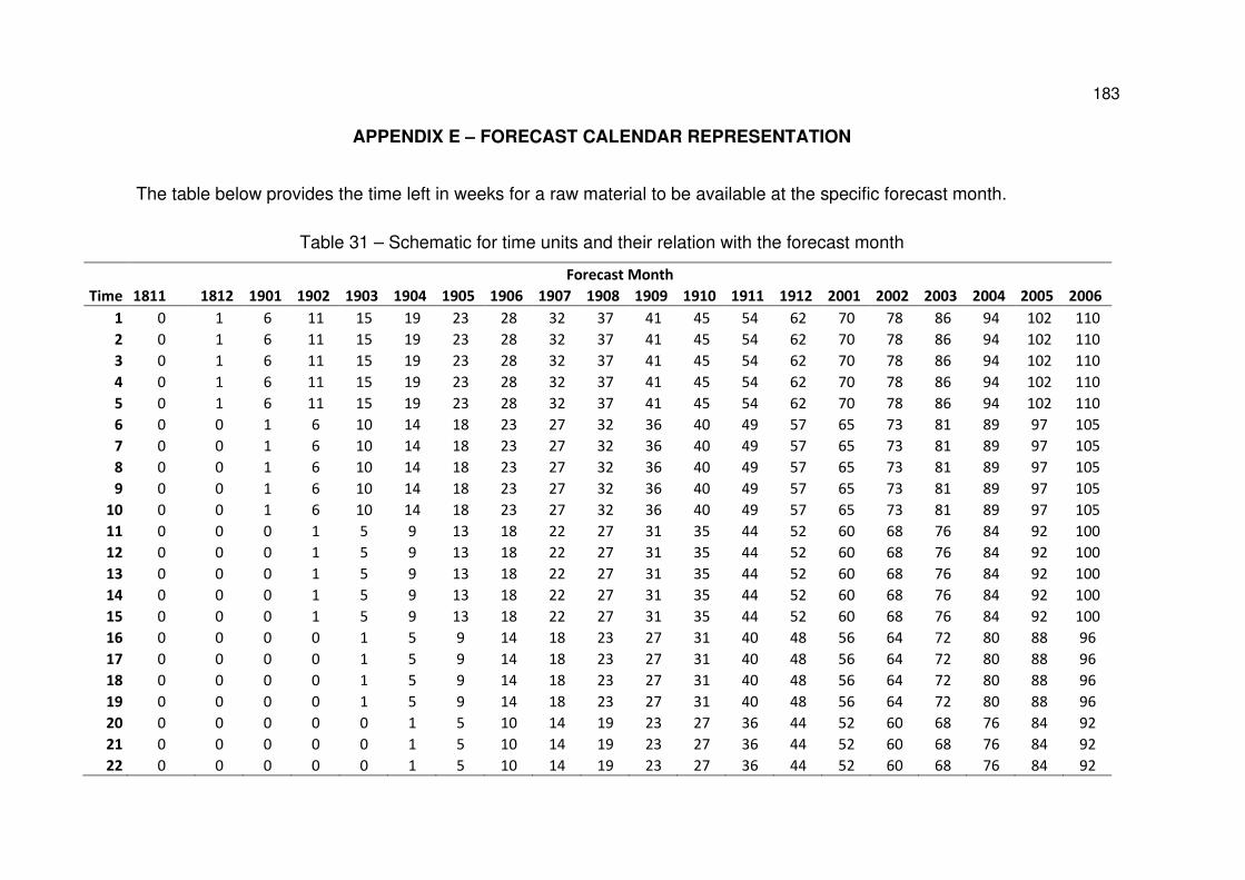
183
APPENDIX E – FORECAST CALENDAR REPRESENTATION
The table below provides the time left in weeks for a raw material to be available at the specific forecast month.
Table 31 – Schematic for time units and their relation with the forecast month
Forecast Month
Time 1811 1812 1901 1902 1903 1904 1905 1906 1907 1908 1909 1910 1911 1912 2001 2002 2003 2004 2005 2006
1 0 1 6 11 15 19 23 28 32 37 41 45 54 62 70 78 86 94 102 110
2 0 1 6 11 15 19 23 28 32 37 41 45 54 62 70 78 86 94 102 110
3 0 1 6 11 15 19 23 28 32 37 41 45 54 62 70 78 86 94 102 110
4 0 1 6 11 15 19 23 28 32 37 41 45 54 62 70 78 86 94 102 110
5 0 1 6 11 15 19 23 28 32 37 41 45 54 62 70 78 86 94 102 110
6 0 0 1 6 10 14 18 23 27 32 36 40 49 57 65 73 81 89 97 105
7 0 0 1 6 10 14 18 23 27 32 36 40 49 57 65 73 81 89 97 105
8 0 0 1 6 10 14 18 23 27 32 36 40 49 57 65 73 81 89 97 105
9 0 0 1 6 10 14 18 23 27 32 36 40 49 57 65 73 81 89 97 105
10 0 0 1 6 10 14 18 23 27 32 36 40 49 57 65 73 81 89 97 105
11 0 0 0 1 5 9 13 18 22 27 31 35 44 52 60 68 76 84 92 100
12 0 0 0 1 5 9 13 18 22 27 31 35 44 52 60 68 76 84 92 100
13 0 0 0 1 5 9 13 18 22 27 31 35 44 52 60 68 76 84 92 100
14 0 0 0 1 5 9 13 18 22 27 31 35 44 52 60 68 76 84 92 100
15 0 0 0 1 5 9 13 18 22 27 31 35 44 52 60 68 76 84 92 100
16 0 0 0 0 1 5 9 14 18 23 27 31 40 48 56 64 72 80 88 96
17 0 0 0 0 1 5 9 14 18 23 27 31 40 48 56 64 72 80 88 96
18 0 0 0 0 1 5 9 14 18 23 27 31 40 48 56 64 72 80 88 96
19 0 0 0 0 1 5 9 14 18 23 27 31 40 48 56 64 72 80 88 96
20 0 0 0 0 0 1 5 10 14 19 23 27 36 44 52 60 68 76 84 92
21 0 0 0 0 0 1 5 10 14 19 23 27 36 44 52 60 68 76 84 92
22 0 0 0 0 0 1 5 10 14 19 23 27 36 44 52 60 68 76 84 92
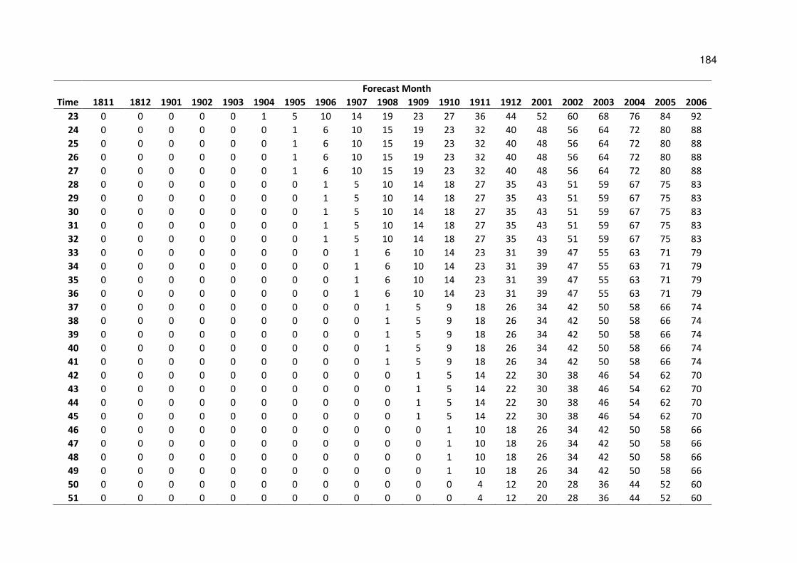
184
Forecast Month
Time 1811 1812 1901 1902 1903 1904 1905 1906 1907 1908 1909 1910 1911 1912 2001 2002 2003 2004 2005 2006
23 0 0 0 0 0 1 5 10 14 19 23 27 36 44 52 60 68 76 84 92
24 0 0 0 0 0 0 1 6 10 15 19 23 32 40 48 56 64 72 80 88
25 0 0 0 0 0 0 1 6 10 15 19 23 32 40 48 56 64 72 80 88
26 0 0 0 0 0 0 1 6 10 15 19 23 32 40 48 56 64 72 80 88
27 0 0 0 0 0 0 1 6 10 15 19 23 32 40 48 56 64 72 80 88
28 0 0 0 0 0 0 0 1 5 10 14 18 27 35 43 51 59 67 75 83
29 0 0 0 0 0 0 0 1 5 10 14 18 27 35 43 51 59 67 75 83
30 0 0 0 0 0 0 0 1 5 10 14 18 27 35 43 51 59 67 75 83
31 0 0 0 0 0 0 0 1 5 10 14 18 27 35 43 51 59 67 75 83
32 0 0 0 0 0 0 0 1 5 10 14 18 27 35 43 51 59 67 75 83
33 0 0 0 0 0 0 0 0 1 6 10 14 23 31 39 47 55 63 71 79
34 0 0 0 0 0 0 0 0 1 6 10 14 23 31 39 47 55 63 71 79
35 0 0 0 0 0 0 0 0 1 6 10 14 23 31 39 47 55 63 71 79
36 0 0 0 0 0 0 0 0 1 6 10 14 23 31 39 47 55 63 71 79
37 0 0 0 0 0 0 0 0 0 1 5 9 18 26 34 42 50 58 66 74
38 0 0 0 0 0 0 0 0 0 1 5 9 18 26 34 42 50 58 66 74
39 0 0 0 0 0 0 0 0 0 1 5 9 18 26 34 42 50 58 66 74
40 0 0 0 0 0 0 0 0 0 1 5 9 18 26 34 42 50 58 66 74
41 0 0 0 0 0 0 0 0 0 1 5 9 18 26 34 42 50 58 66 74
42 0 0 0 0 0 0 0 0 0 0 1 5 14 22 30 38 46 54 62 70
43 0 0 0 0 0 0 0 0 0 0 1 5 14 22 30 38 46 54 62 70
44 0 0 0 0 0 0 0 0 0 0 1 5 14 22 30 38 46 54 62 70
45 0 0 0 0 0 0 0 0 0 0 1 5 14 22 30 38 46 54 62 70
46 0 0 0 0 0 0 0 0 0 0 0 1 10 18 26 34 42 50 58 66
47 0 0 0 0 0 0 0 0 0 0 0 1 10 18 26 34 42 50 58 66
48 0 0 0 0 0 0 0 0 0 0 0 1 10 18 26 34 42 50 58 66
49 0 0 0 0 0 0 0 0 0 0 0 1 10 18 26 34 42 50 58 66
50 0 0 0 0 0 0 0 0 0 0 0 0 4 12 20 28 36 44 52 60
51 0 0 0 0 0 0 0 0 0 0 0 0 4 12 20 28 36 44 52 60
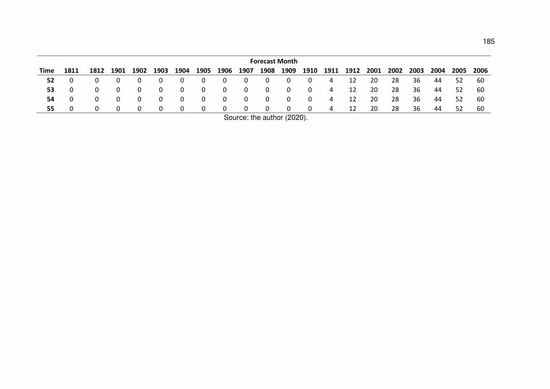
185
Forecast Month
Time 1811 1812 1901 1902 1903 1904 1905 1906 1907 1908 1909 1910 1911 1912 2001 2002 2003 2004 2005 2006
52 0 0 0 0 0 0 0 0 0 0 0 0 4 12 20 28 36 44 52 60
53 0 0 0 0 0 0 0 0 0 0 0 0 4 12 20 28 36 44 52 60
54 0 0 0 0 0 0 0 0 0 0 0 0 4 12 20 28 36 44 52 60
55 0 0 0 0 0 0 0 0 0 0 0 0 4 12 20 28 36 44 52 60
Source: the author (2020).
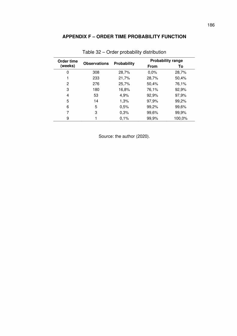
186
APPENDIX F – ORDER TIME PROBABILITY FUNCTION
Table 32 – Order probability distribution
Order time (weeks)
Observations Probability Probability range
From To
0 308 28,7% 0,0% 28,7% 1 233 21,7% 28,7% 50,4% 2 276 25,7% 50,4% 76,1% 3 180 16,8% 76,1% 92,9% 4 53 4,9% 92,9% 97,9% 5 14 1,3% 97,9% 99,2% 6 5 0,5% 99,2% 99,6% 7 3 0,3% 99,6% 99,9% 9 1 0,1% 99,9% 100,0%
Source: the author (2020).
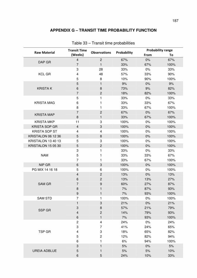
187
APPENDIX G – TRANSIT TIME PROBABILITY FUNCTION
Table 33 – Transit time probabilities
Raw Material Transit Time
(Weeks) Observations Probability
Probability range
From To
DAP GR 4 2 67% 0% 67%
7 1 33% 67% 100%
KCL GR 3 28 33% 0% 33% 4 48 57% 33% 90%
5 8 10% 90% 100%
KRISTA K
5 1 9% 0% 9%
6 8 73% 9% 82% 7 2 18% 82% 100%
KRISTA MAG 5 1 33% 0% 33% 6 1 33% 33% 67% 8 1 33% 67% 100%
KRISTA MAP 7 2 67% 0% 67% 8 1 33% 67% 100%
KRISTA MKP 11 3 100% 0% 100% KRISTA SOP GR 4 3 100% 0% 100% KRISTA SOP ST 4 4 100% 0% 100%
KRISTALON 06 12 36 5 8 100% 0% 100% KRISTALON 13 40 13 5 3 100% 0% 100%
KRISTALON 15 05 30 5 2 100% 0% 100%
NAM
3 1 33% 0% 33%
5 1 33% 33% 67% 7 1 33% 67% 100%
NIP GR 6 3 100% 0% 100%
PG MIX 14 16 18 5 6 100% 0% 100%
SAM GR
4 2 13% 0% 13%
6 2 13% 13% 27% 7 9 60% 27% 87% 8 1 7% 87% 93%
9 1 7% 93% 100% SAM STD 7 1 100% 0% 100%
SSP GR
1 3 21% 0% 21% 3 8 57% 21% 79%
4 2 14% 79% 93% 6 1 7% 93% 100%
TSP GR
2 4 24% 0% 24%
3 7 41% 24% 65% 4 3 18% 65% 82%
5 2 12% 82% 94% 6 1 6% 94% 100%
UREIA ADBLUE
3 1 5% 0% 5%
5 1 5% 5% 10% 6 5 24% 10% 33%
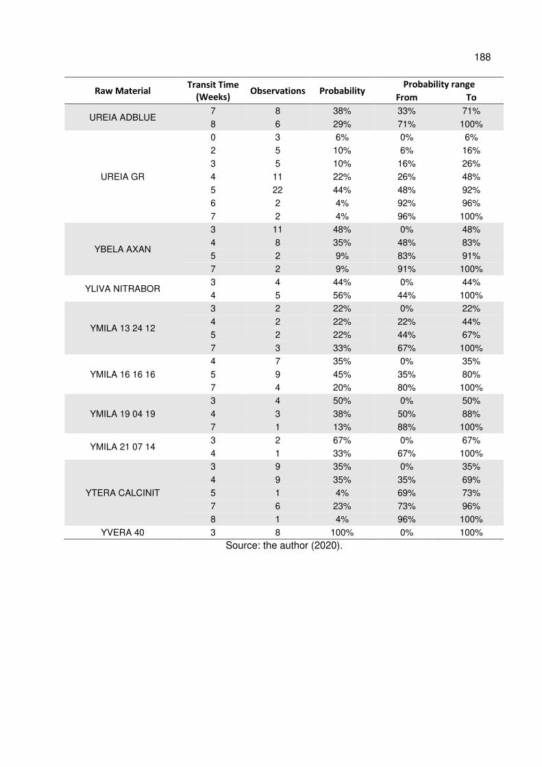
188
Raw Material Transit Time
(Weeks) Observations Probability
Probability range
From To
UREIA ADBLUE 7 8 38% 33% 71%
8 6 29% 71% 100%
UREIA GR
0 3 6% 0% 6% 2 5 10% 6% 16%
3 5 10% 16% 26% 4 11 22% 26% 48%
5 22 44% 48% 92% 6 2 4% 92% 96%
7 2 4% 96% 100%
YBELA AXAN
3 11 48% 0% 48% 4 8 35% 48% 83%
5 2 9% 83% 91% 7 2 9% 91% 100%
YLIVA NITRABOR 3 4 44% 0% 44% 4 5 56% 44% 100%
YMILA 13 24 12
3 2 22% 0% 22%
4 2 22% 22% 44% 5 2 22% 44% 67%
7 3 33% 67% 100%
YMILA 16 16 16
4 7 35% 0% 35%
5 9 45% 35% 80% 7 4 20% 80% 100%
YMILA 19 04 19
3 4 50% 0% 50%
4 3 38% 50% 88% 7 1 13% 88% 100%
YMILA 21 07 14 3 2 67% 0% 67% 4 1 33% 67% 100%
YTERA CALCINIT
3 9 35% 0% 35%
4 9 35% 35% 69% 5 1 4% 69% 73%
7 6 23% 73% 96% 8 1 4% 96% 100%
YVERA 40 3 8 100% 0% 100% Source: the author (2020).
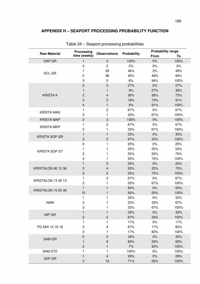
189
APPENDIX H – SEAPORT PROCESSING PROBABILITY FUNCTION
Table 34 – Seaport processing probabilities
Raw Material Processing
time (weeks) Observations Probability
Probability range
From To
DAP GR 1 3 100% 0% 100%
KCL GR
0 2 2% 0% 2% 1 39 46% 2% 49% 2 38 45% 49% 94%
3 5 6% 94% 100%
KRISTA K
0 3 27% 0% 27%
1 1 9% 27% 36% 2 4 36% 36% 73%
3 2 18% 73% 91% 4 1 9% 91% 100%
KRISTA MAG 1 2 67% 0% 67%
2 1 33% 67% 100% KRISTA MAP 2 3 100% 0% 100%
KRISTA MKP 1 2 67% 0% 67% 2 1 33% 67% 100%
KRISTA SOP GR 1 1 33% 0% 33%
3 2 67% 33% 100%
KRISTA SOP ST
0 1 25% 0% 25%
1 1 25% 25% 50% 2 1 25% 50% 75%
4 1 25% 75% 100%
KRISTALON 06 12 36 1 2 25% 0% 25% 2 4 50% 25% 75%
3 2 25% 75% 100%
KRISTALON 13 40 13 1 2 67% 0% 67%
3 1 33% 67% 100%
KRISTALON 15 05 30 1 1 50% 0% 50%
10 1 50% 50% 100%
NAM 1 1 33% 0% 33% 2 1 33% 33% 67%
3 1 33% 67% 100%
NIP GR 1 1 33% 0% 33%
2 2 67% 33% 100%
PG MIX 14 16 18 1 1 17% 0% 17% 2 4 67% 17% 83%
3 1 17% 83% 100%
SAM GR 0 5 33% 0% 33%
1 9 60% 33% 93% 2 1 7% 93% 100%
SAM STD 1 1 100% 0% 100%
SSP GR 1 4 29% 0% 29% 2 10 71% 29% 100%
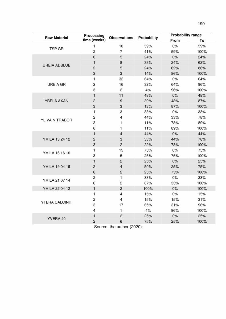
190
Raw Material Processing
time (weeks) Observations Probability
Probability range
From To
TSP GR 1 10 59% 0% 59%
2 7 41% 59% 100%
UREIA ADBLUE
0 5 24% 0% 24% 1 8 38% 24% 62%
2 5 24% 62% 86% 3 3 14% 86% 100%
UREIA GR 1 32 64% 0% 64% 2 16 32% 64% 96%
3 2 4% 96% 100%
YBELA AXAN 1 11 48% 0% 48% 2 9 39% 48% 87%
3 3 13% 87% 100%
YLIVA NITRABOR
1 3 33% 0% 33%
2 4 44% 33% 78% 3 1 11% 78% 89% 6 1 11% 89% 100%
YMILA 13 24 12 1 4 44% 0% 44% 2 3 33% 44% 78%
3 2 22% 78% 100%
YMILA 16 16 16 1 15 75% 0% 75%
3 5 25% 75% 100%
YMILA 19 04 19 1 2 25% 0% 25% 2 4 50% 25% 75%
6 2 25% 75% 100%
YMILA 21 07 14 2 1 33% 0% 33%
6 2 67% 33% 100% YMILA 22 04 12 1 2 100% 0% 100%
YTERA CALCINIT
1 4 15% 0% 15%
2 4 15% 15% 31% 3 17 65% 31% 96%
4 1 4% 96% 100%
YVERA 40 1 2 25% 0% 25%
2 6 75% 25% 100% Source: the author (2020).
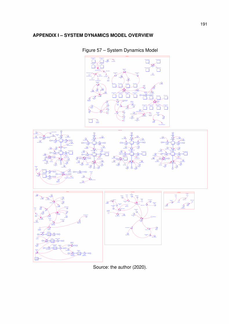
191
APPENDIX I – SYSTEM DYNAMICS MODEL OVERVIEW
Figure 57 – System Dynamics Model
Source: the author (2020).
Lead Times
Supply Chain
Measures
PlanningTOC planning
POA Inventory
Transfer inventory
CAN
RIG Inventory
Transfer inventory
POA
Total realized RIG
Transfer Inventory
RIG
CZB Inventory
Transfer Inventory
RIG
Creating PO
RIG Inventory
Transfer inventory
CAN
CZB Inventory
Transfer Inventory
RIG
In transit
Total realized CZB
Planned purchases
Processing RM
at seaport
CZB InventoryRIG Inventory
Total realized POA
Transfer inventory
CZB
Transfer inventory
CAN
POA Inventory
Creating PO
Transfer inventory
POA
Total realized CZB
Transfer inventory
POA
Total realized CAN
Transfer Inventory
RIG
Shipping to
units
Transferred POA
Total realized POA
Planned purchases
Future purchases
CAN Inventory
Total realized RIG
Transfer inventory
CZB
Transfer inventory
POA
Transfer inventory
CZB
CAN Inventory
Transfer inventory
CAN
CAN Inventory
POA Inventory
Transfer inventory
CZB
Total realized CAN
Total recebido
Total realized
Unmet demand
POA
Unmet demand
RIG
Unmet demand
CZB
Unmet demand
CAN
Total inventory in the unit
Total Inventory
Total transfer Inventory
TOC Buffer
penetration
TOC re-order - NF
Total inventory
RM
Total unmet
demand
RM re-order
quantity
Buffer size
Buffer level
RM re-order
quantity
Total Realized
RM
Realized per
Month
Incoming transfer
RIG
Transit time
Forecast
Random TT
Incoming transfers
CAN
Exposure
Forecast
Calendar
RM Forecast
Total purchases
RM
Re-order
quantity
Exposure RM
Incoming transfers POA
Month Indicator
Transit time
premise
Port time premise
Total purchases
RM
Incoming transfers CZB
Realized per
Month RM
Supply premise
Acum Forecast
Supply premise
Realized transfers
ETA
Available at
requesting unit
Total LT Premise
Purchased
RM
Total inventory CZB
Total purchases
RM
Order LT
premise
Total inventory POA
Batch premise
Re-order point
Realized transfers
Total inventory RIG
Total available
Realized transfers
Realized
CAN
Re-ordering RM
Random PO
PO Time
Supply premise
Sending PO
Stock Aggr
Receiving PO
Realized
CAN
Arriving at seaport
Waiting at seaport
Random
seaport
Seaport
processing time
Realized CZB
Available at
seaport
Realized POA
Purchased
RM
Supply premise
Total inventory CAN
Available at
seaport unit
Realized RIG
To be shipped to
requesting unit
Available at
seaport unit
Acc RM inventory
Stock Aggr
acc inventory
Realized CZB
Avg total
inventory
Realized POA
Avg RM
inventory
Realized transfers
Available at
requesting unit
Safety
stock
Avg coverage RM
Acc RM
purchases
Stock Aggr
Stock Aggr
Supply premise
Realized RIG
Transfer order POA
TT seed
Transfer order CAN
PO seed
Supply premise
Seaport seed
Supply premise
RM price
IDD
TDD
Transfer CZB
- RIG
Transfer POA
- CZB
Delayed
time
Transfer RIG -
CZB
Transfer CZB
- POA
RM TDD
Unit TDD
Total TDD
Transfer RIG
- CAN
Transfer order CAN
Transfer order RIG
RM Inventory
per plant
Total realized
per plant
Inventory
value
Transfer CAN
- CZBTransfer POA
- CAN
Daily unit
consumption
Days on
hand
Transfer RIG
- POA
Total transfer
orders
Supply premise
RM IDD
Unit IDD
Total IDD
Transfer POA
- RIG
Transfer order RIG
Transfer order CZB
Daily
consumption
Total transfer
orders
Supply premise
TOC RLT
Total transfer
orders
Buffer size FB
Transfer CAN
- RIG
Transfer CAN
- POA
TOC Re-order
quantity
Total available
Transfer order POA
TOC ETA
Transfer order RIG
Transfer order RIG
TOC Re-order
point
Total transfer
orders
Transfer order CZB
TOC Re-order FB
Received orders
RIG
Transfer CZB
- CAN
Total available
Total available
Transfer order POA
RM Re-order
quantity - FB
TOC Buffer
Transfer order CZB
Purchase
frequency
Purchase
quantity
Total purchase frequency
Transfer order POA
Transfer frequency
Total transfer
frequency
Transfer order CAN
Total planned
purchases
Avg
consumption
Buffer type
Max time
Total available
Supply premise
TOC Buffer
penetration
Buffer indicator
Transfer order CAN
Buffer size
Transfer order CZB
TOC re-order - NF
RM Re-order
quantity - NF
RM re-order
quantity
Buffer zone
Buffer level
Dynamic
buffer
Realized
CAN
Realized CZB
Committed
purchases
Transfer RIG
- POA
Transfer RIG -
CZB
Transfer order RIG
Transfer RIG
- CAN
Available RIG
Outgoing transfers
RIG
Available
Transfer order POA
Available CAN
Transfer POA
- RIG
Transfer order CAN
Transfer CZB
- RIG
Transfer POA
- CAN
Transfer POA
- CZB
Outgoing transfers CAN
Realized RIG
Future purchases
available
Outgoing transfers POA Outgoing transfers CZB
Realized POA
Transfer CAN
- CZB
Transfer CAN
- POA
Transfer order CZB
Incoming transfers CZBIncoming transfers
CAN
Incoming transfers POA
Available CZB
Realized transfers
Available POA
Incoming transfer
RIG
Total available
Transfer CZB
- CAN
Transfer CZB
- POA
Total transfer
orders
Transfer CAN
- RIG
Total puchased
Aggregated inventory
Supply unit
Total purchases
RM
TOC RLT
Planning simulation
Stock Aggr
Received orders
RIG
Total inventory RIG
Received orders
CZB
Total inventory CZB
Received orders
CAN
Supply premise
Total inventory CAN
Received orders
POA
Total inventory POA
Max re-order
time
Total inventory
RM
Realized per
Month
RM Forecast
Total unmet
demand
RM Inventory
per plant
Acum Forecast
Realized per
Month
Total inventory
RM
Forecast
Calendar
Total LT Premise
TOC RLT
TOC Re-order FB
Batch premise
Total inventory
RM
Batch premise
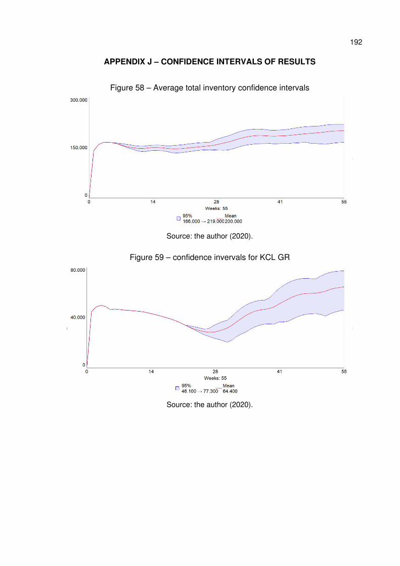
192
APPENDIX J – CONFIDENCE INTERVALS OF RESULTS
Figure 58 – Average total inventory confidence intervals
Source: the author (2020).
Figure 59 – confidence invervals for KCL GR
Source: the author (2020).
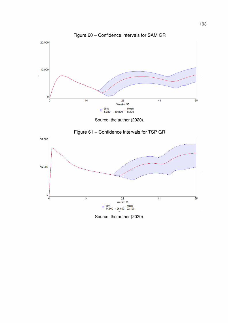
193
Figure 60 – Confidence intervals for SAM GR
Source: the author (2020).
Figure 61 – Confidence intervals for TSP GR
Source: the author (2020).
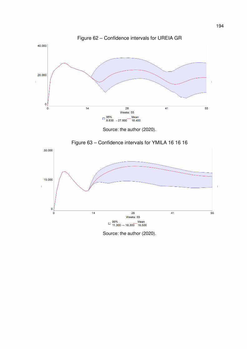
194
Figure 62 – Confidence intervals for UREIA GR
Source: the author (2020).
Figure 63 – Confidence intervals for YMILA 16 16 16
Source: the author (2020).
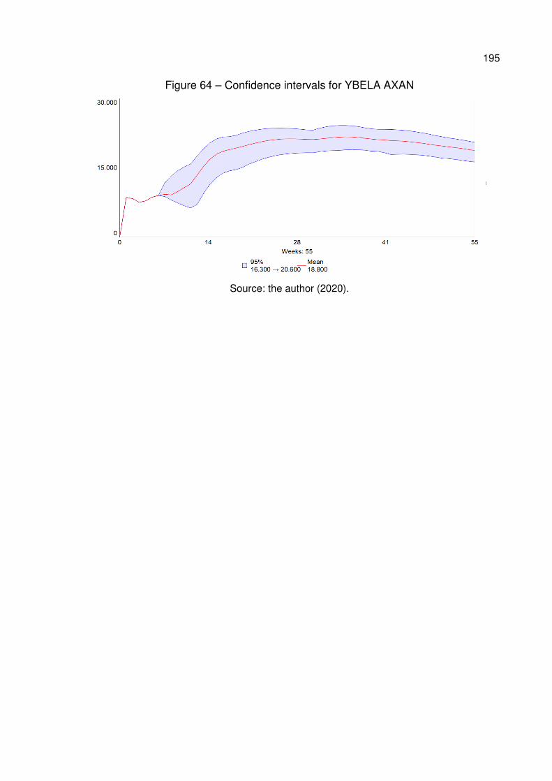
195
Figure 64 – Confidence intervals for YBELA AXAN
Source: the author (2020).
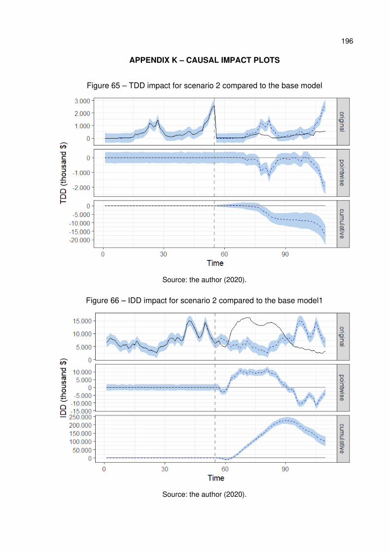
196
APPENDIX K – CAUSAL IMPACT PLOTS
Figure 65 – TDD impact for scenario 2 compared to the base model
Source: the author (2020).
Figure 66 – IDD impact for scenario 2 compared to the base model1
Source: the author (2020).
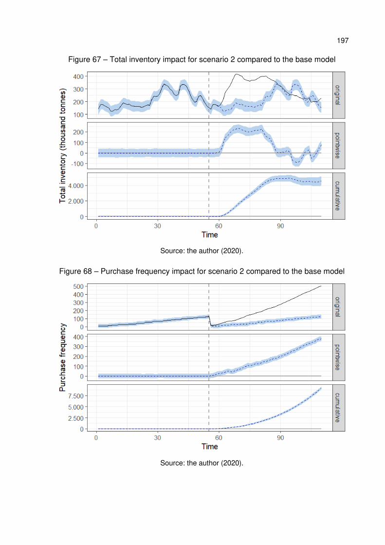
197
Figure 67 – Total inventory impact for scenario 2 compared to the base model
Source: the author (2020).
Figure 68 – Purchase frequency impact for scenario 2 compared to the base model
Source: the author (2020).
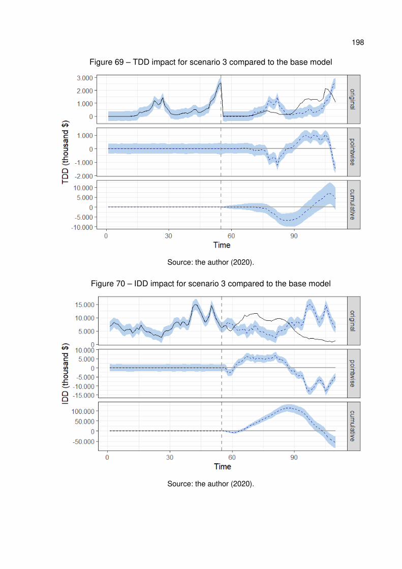
198
Figure 69 – TDD impact for scenario 3 compared to the base model
Source: the author (2020).
Figure 70 – IDD impact for scenario 3 compared to the base model
Source: the author (2020).
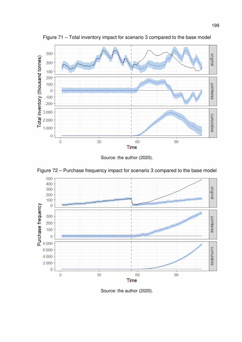
199
Figure 71 – Total inventory impact for scenario 3 compared to the base model
Source: the author (2020).
Figure 72 – Purchase frequency impact for scenario 3 compared to the base model
Source: the author (2020).
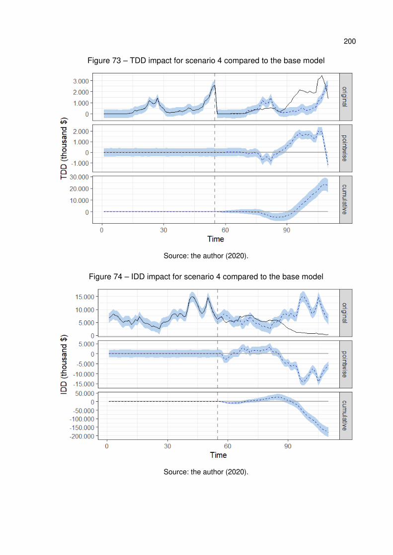
200
Figure 73 – TDD impact for scenario 4 compared to the base model
Source: the author (2020).
Figure 74 – IDD impact for scenario 4 compared to the base model
Source: the author (2020).
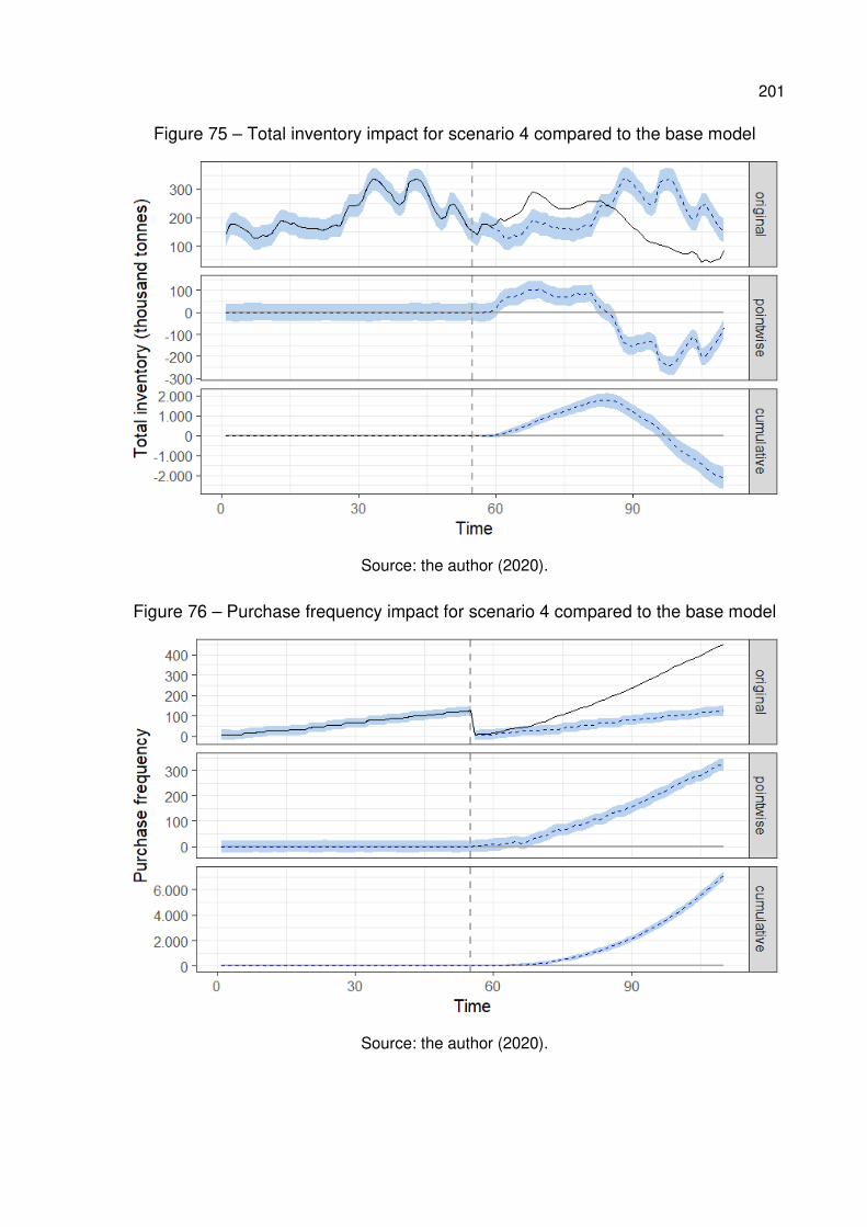
201
Figure 75 – Total inventory impact for scenario 4 compared to the base model
Source: the author (2020).
Figure 76 – Purchase frequency impact for scenario 4 compared to the base model
Source: the author (2020).
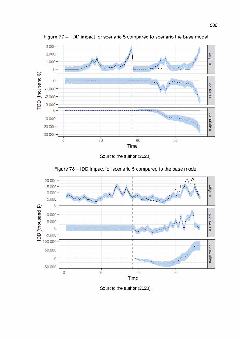
202
Figure 77 – TDD impact for scenario 5 compared to scenario the base model
Source: the author (2020).
Figure 78 – IDD impact for scenario 5 compared to the base model
Source: the author (2020).
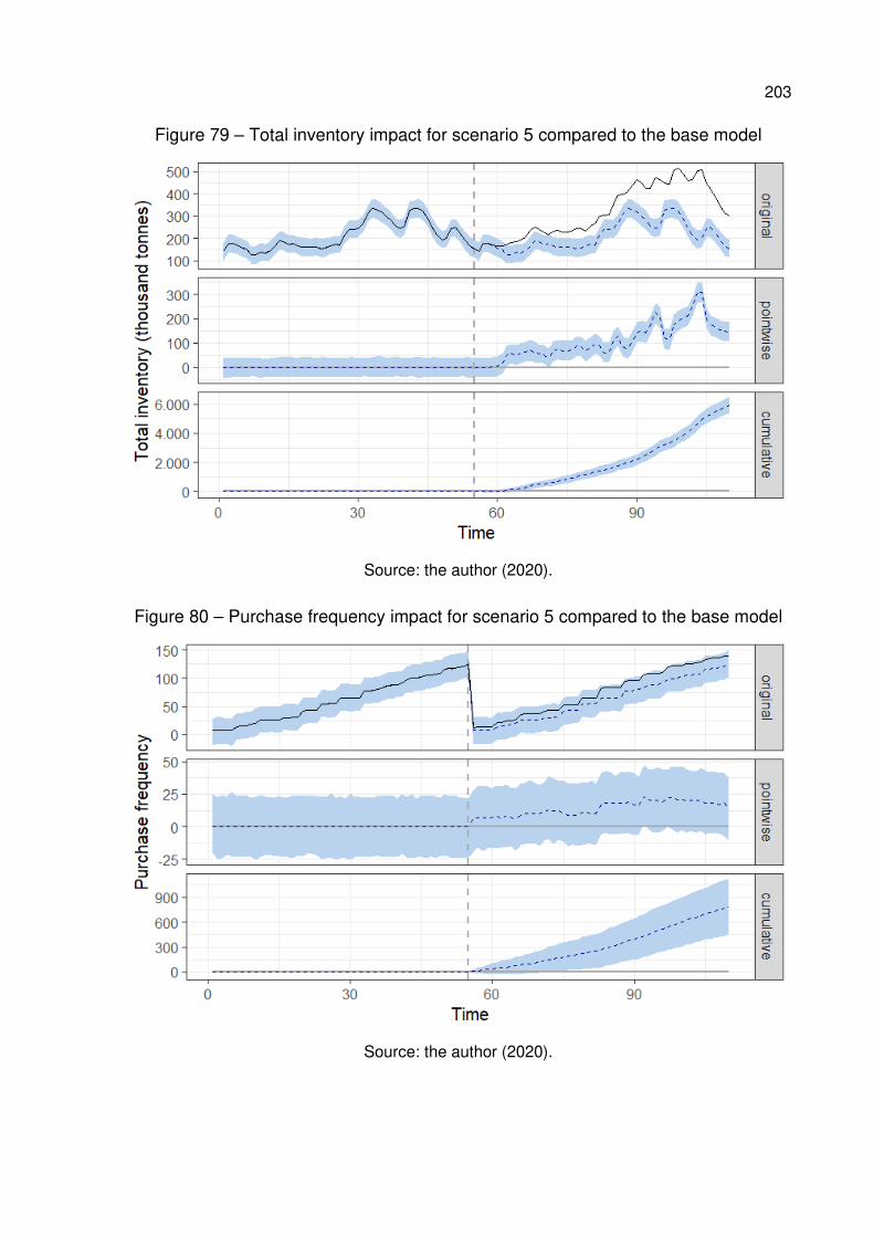
203
Figure 79 – Total inventory impact for scenario 5 compared to the base model
Source: the author (2020).
Figure 80 – Purchase frequency impact for scenario 5 compared to the base model
Source: the author (2020).
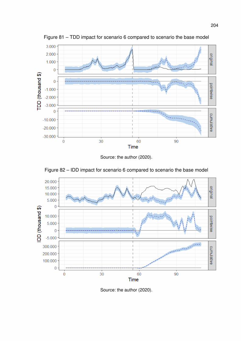
204
Figure 81 – TDD impact for scenario 6 compared to scenario the base model
Source: the author (2020).
Figure 82 – IDD impact for scenario 6 compared to scenario the base model
Source: the author (2020).
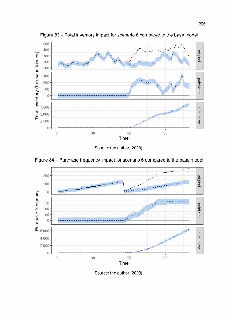
205
Figure 83 – Total inventory impact for scenario 6 compared to the base model
Source: the author (2020).
Figure 84 – Purchase frequency impact for scenario 6 compared to the base model
Source: the author (2020).
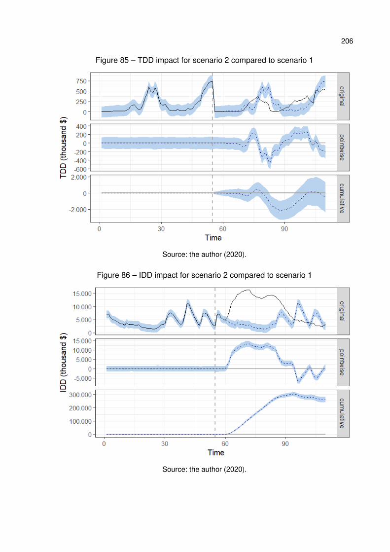
206
Figure 85 – TDD impact for scenario 2 compared to scenario 1
Source: the author (2020).
Figure 86 – IDD impact for scenario 2 compared to scenario 1
Source: the author (2020).
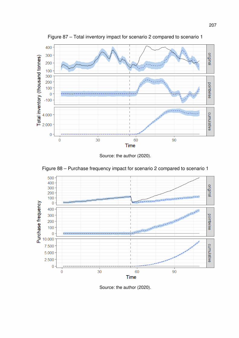
207
Figure 87 – Total inventory impact for scenario 2 compared to scenario 1
Source: the author (2020).
Figure 88 – Purchase frequency impact for scenario 2 compared to scenario 1
Source: the author (2020).
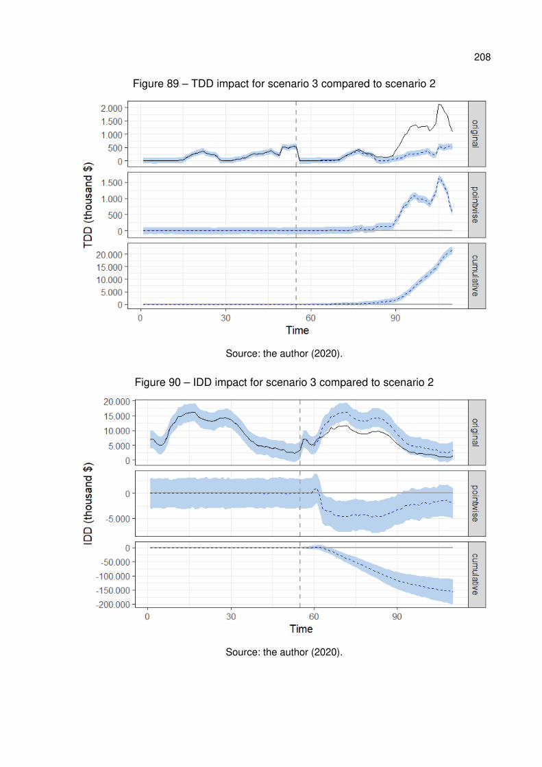
208
Figure 89 – TDD impact for scenario 3 compared to scenario 2
Source: the author (2020).
Figure 90 – IDD impact for scenario 3 compared to scenario 2
Source: the author (2020).
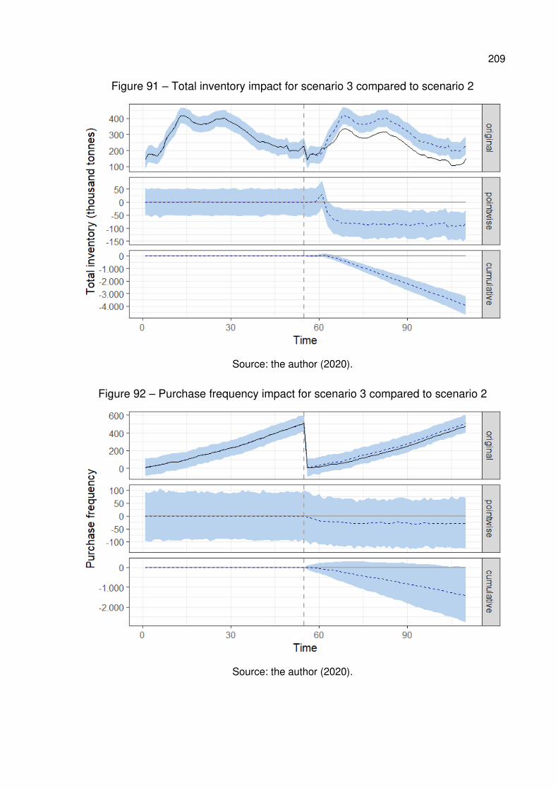
209
Figure 91 – Total inventory impact for scenario 3 compared to scenario 2
Source: the author (2020).
Figure 92 – Purchase frequency impact for scenario 3 compared to scenario 2
Source: the author (2020).
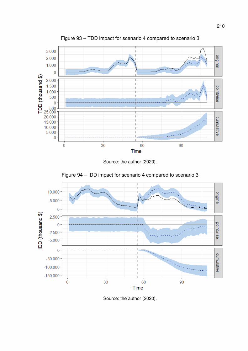
210
Figure 93 – TDD impact for scenario 4 compared to scenario 3
Source: the author (2020).
Figure 94 – IDD impact for scenario 4 compared to scenario 3
Source: the author (2020).
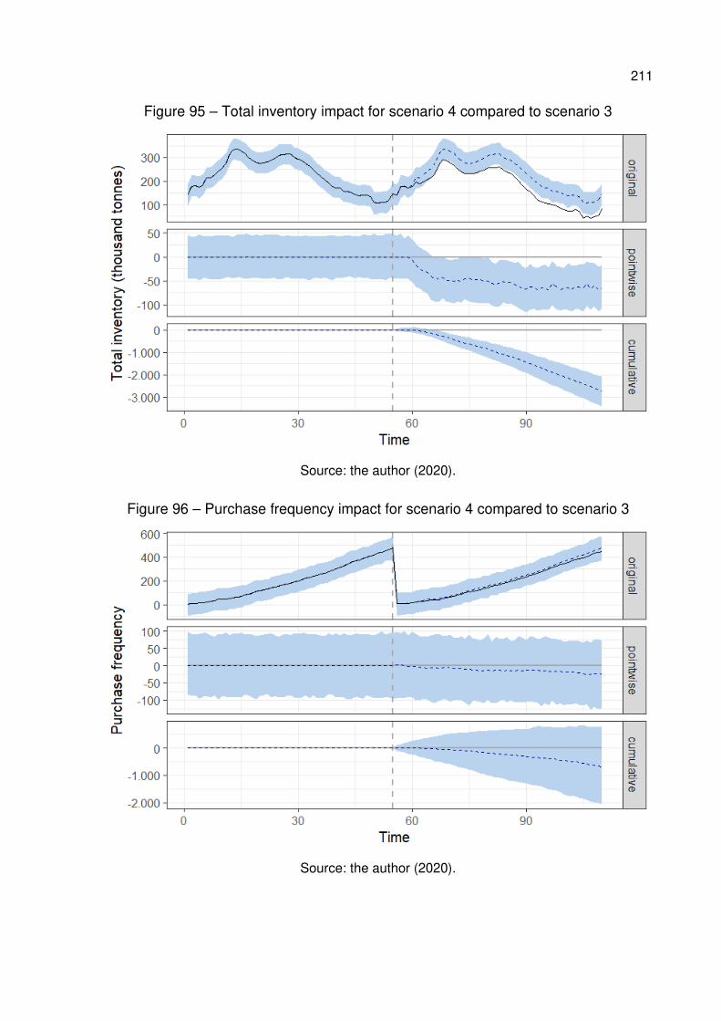
211
Figure 95 – Total inventory impact for scenario 4 compared to scenario 3
Source: the author (2020).
Figure 96 – Purchase frequency impact for scenario 4 compared to scenario 3
Source: the author (2020).
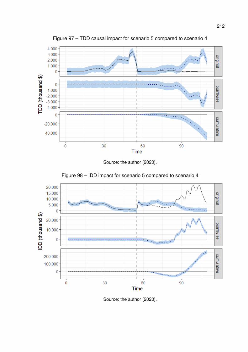
212
Figure 97 – TDD causal impact for scenario 5 compared to scenario 4
Source: the author (2020).
Figure 98 – IDD impact for scenario 5 compared to scenario 4
Source: the author (2020).
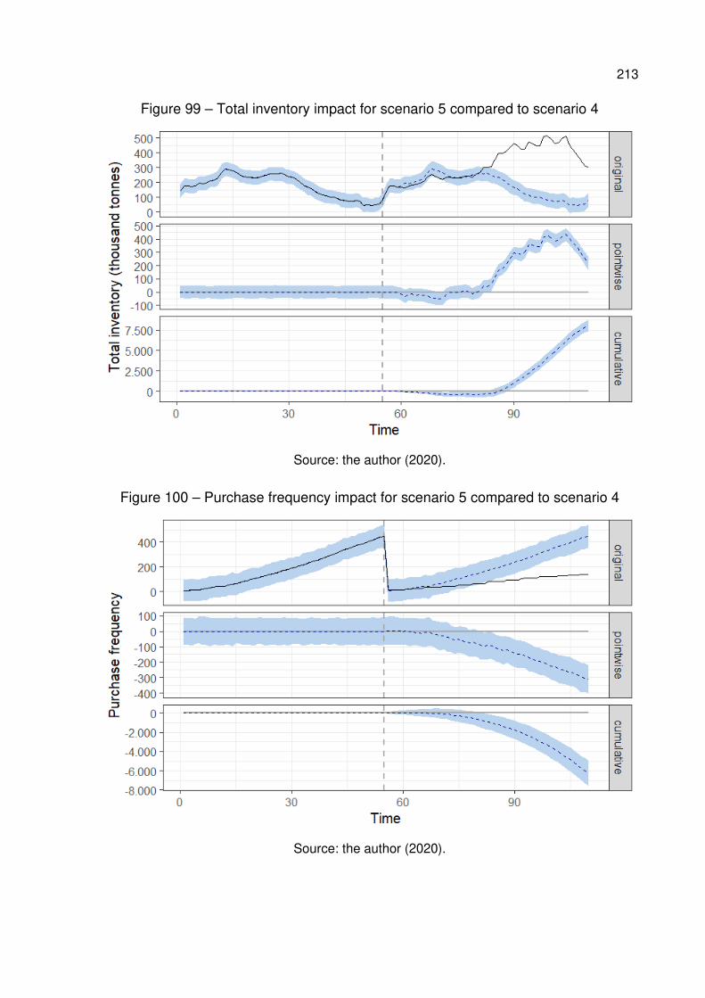
213
Figure 99 – Total inventory impact for scenario 5 compared to scenario 4
Source: the author (2020).
Figure 100 – Purchase frequency impact for scenario 5 compared to scenario 4
Source: the author (2020).
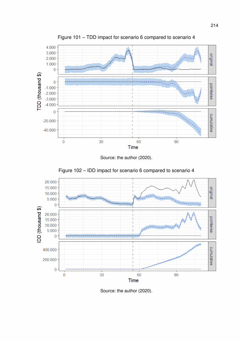
214
Figure 101 – TDD impact for scenario 6 compared to scenario 4
Source: the author (2020).
Figure 102 – IDD impact for scenario 6 compared to scenario 4
Source: the author (2020).
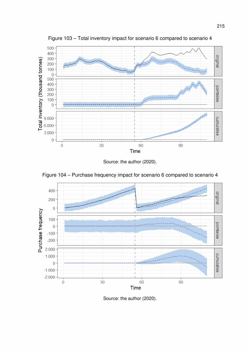
215
Figure 103 – Total inventory impact for scenario 6 compared to scenario 4
Source: the author (2020).
Figure 104 – Purchase frequency impact for scenario 6 compared to scenario 4
Source: the author (2020).
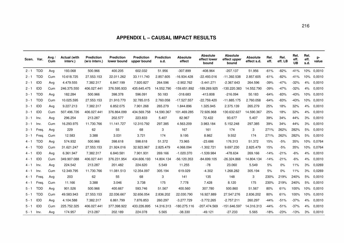
216
APPENDIX L – CAUSAL IMPACT RESULTS
Scen. Var. Avg / Cum
Actual (with interv.)
Prediction (w/o interv.)
Prediction lower bound
Prediction upper bound
Prediction s.d.
Absolute effect
Absolute effect lower
bound
Absolute effect upper
bound
Absolute effect s.d.
Rel. eff.
Rel. eff. LB
Rel. eff. UB
Rel. eff. s.d.
p-value
2 - 1 TDD Avg 193.068 500.966 400.205 602.032 51.956 -307.899 -408.964 -207.137 51.956 -61% -82% -41% 10% 0,0010
2 - 1 TDD Cum 10.618.725 27.553.153 22.011.262 33.111.740 2.857.605 -16.934.428 -22.493.016 -11.392.538 2.857.605 -61% -82% -41% 10% 0,0010
2 - 1 IDD Avg 4.479.555 7.382.317 6.847.199 7.920.827 264.596 -2.902.762 -3.441.271 -2.367.643 264.596 -39% -47% -32% 4% 0,0010
2 - 1 IDD Cum 246.375.550 406.027.441 376.595.933 435.645.475 14.552.790 -159.651.892 -189.269.925 -130.220.383 14.552.790 -39% -47% -32% 4% 0,0010
3 - 1 TDD Avg 182.284 500.966 398.378 596.091 50.183 -318.683 -413.808 -216.094 50.183 -64% -83% -43% 10% 0,0010
3 - 1 TDD Cum 10.025.595 27.553.153 21.910.770 32.785.015 2.760.058 -17.527.557 -22.759.420 -11.885.175 2.760.058 -64% -83% -43% 10% 0,0010
3 - 1 IDD Avg 9.227.213 7.382.317 6.852.075 7.901.268 265.279 1.844.896 1.325.945 2.375.139 265.279 25% 18% 32% 4% 0,0010
3 - 1 IDD Cum 507.496.726 406.027.441 376.864.099 434.569.758 14.590.367 101.469.285 72.926.968 130.632.627 14.590.367 25% 18% 32% 4% 0,0010
3 - 1 Inv. Avg 296.254 213.287 202.577 223.833 5.407 82.967 72.422 93.677 5.407 39% 34% 44% 3% 0,0010
3 - 1 Inv. Cum 16.293.975 11.730.766 11.141.727 12.310.792 297.385 4.563.209 3.983.184 5.152.248 297.385 39% 34% 44% 3% 0,0010
3 - 1 Freq. Avg 229 62 55 68 3 167 161 174 3 271% 262% 282% 5% 0,0010
3 - 1 Freq. Cum 12.583 3.388 3.031 3.721 174 9.195 8.862 9.552 174 271% 262% 282% 5% 0,0010
4 - 1 TDD Avg 574.932 500.966 398.618 598.618 51.372 73.965 -23.686 176.313 51.372 15% -5% 35% 10% 0,0764
4 - 1 TDD Cum 31.621.247 27.553.153 21.924.016 32.923.967 2.825.479 4.068.094 -1.302.721 9.697.230 2.825.479 15% -5% 35% 10% 0,0764
4 - 1 IDD Avg 6.361.947 7.382.317 6.840.581 7.901.931 269.166 -1.020.370 -1.539.984 -478.634 269.166 -14% -21% -6% 4% 0,0010
4 - 1 IDD Cum 349.907.088 406.027.441 376.231.954 434.606.193 14.804.134 -56.120.353 -84.699.105 -26.324.866 14.804.134 -14% -21% -6% 4% 0,0010
4 - 1 Inv. Avg 224.542 213.287 201.482 224.620 5.549 11.255 -78 23.060 5.549 5% 0% 11% 3% 0,0269
4 - 1 Inv. Cum 12.349.795 11.730.766 11.081.513 12.354.097 305.194 619.029 -4.302 1.268.282 305.194 5% 0% 11% 3% 0,0269
4 - 1 Freq. Avg 203 62 55 68 3 141 135 148 3 230% 219% 240% 5% 0,0010
4 - 1 Freq. Cum 11.166 3.388 3.046 3.738 175 7.778 7.428 8.120 175 230% 219% 240% 5% 0,0010
5 - 1 TDD Avg 901.526 500.966 400.667 593.746 51.567 400.560 307.780 500.860 51.567 80% 61% 100% 10% 0,0010
5 - 1 TDD Cum 49.583.943 27.553.153 22.036.667 32.656.054 2.836.202 22.030.790 16.927.889 27.547.276 2.836.202 80% 61% 100% 10% 0,0010
5 - 1 IDD Avg 4.104.588 7.382.317 6.861.799 7.876.853 260.297 -3.277.729 -3.772.265 -2.757.211 260.297 -44% -51% -37% 4% 0,0010
5 - 1 IDD Cum 225.752.325 406.027.441 377.398.922 433.226.895 14.316.313 -180.275.116 -207.474.569 -151.646.597 14.316.313 -44% -51% -37% 4% 0,0010
5 - 1 Inv. Avg 174.957 213.287 202.189 224.078 5.565 -38.330 -49.121 -27.233 5.565 -18% -23% -13% 3% 0,0010
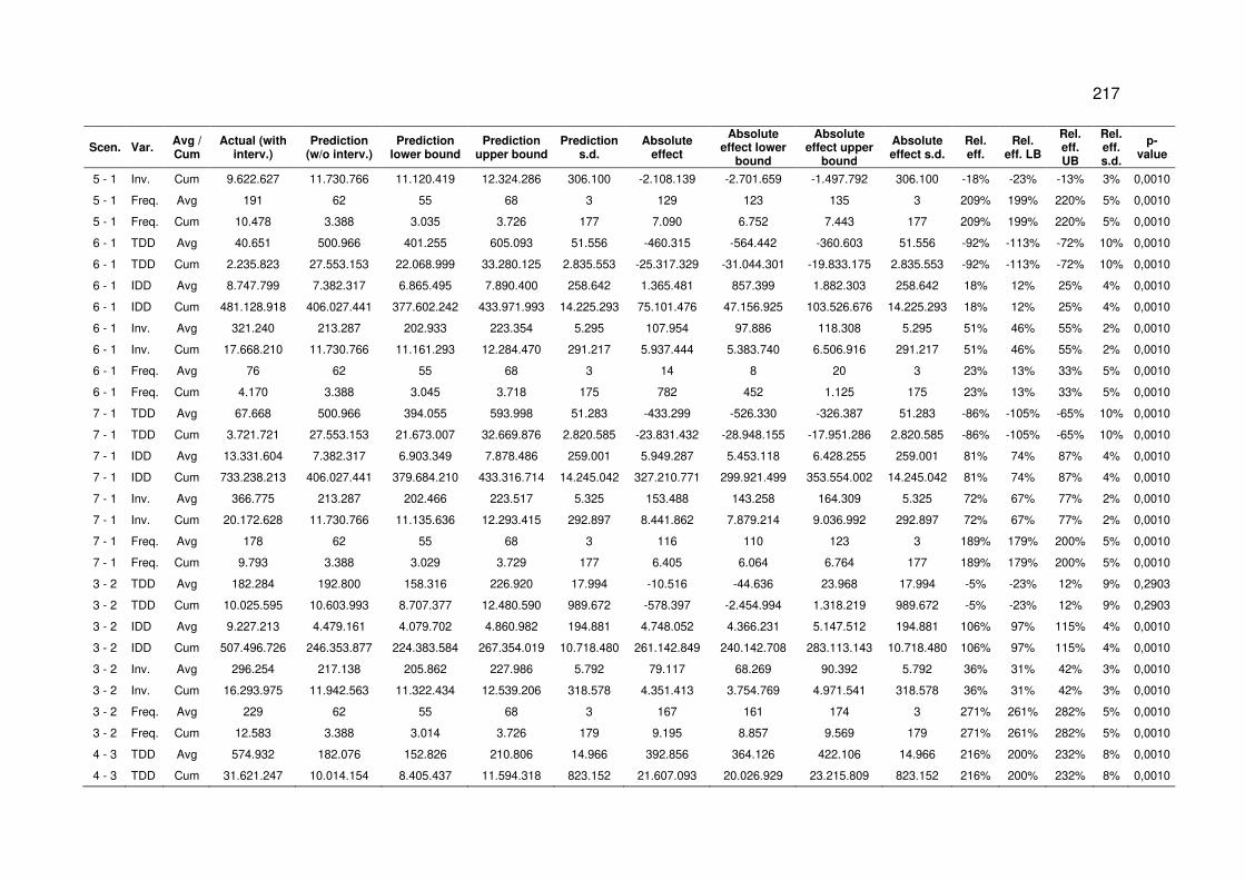
217
Scen. Var. Avg / Cum
Actual (with interv.)
Prediction (w/o interv.)
Prediction lower bound
Prediction upper bound
Prediction s.d.
Absolute effect
Absolute effect lower
bound
Absolute effect upper
bound
Absolute effect s.d.
Rel. eff.
Rel. eff. LB
Rel. eff. UB
Rel. eff. s.d.
p-value
5 - 1 Inv. Cum 9.622.627 11.730.766 11.120.419 12.324.286 306.100 -2.108.139 -2.701.659 -1.497.792 306.100 -18% -23% -13% 3% 0,0010
5 - 1 Freq. Avg 191 62 55 68 3 129 123 135 3 209% 199% 220% 5% 0,0010
5 - 1 Freq. Cum 10.478 3.388 3.035 3.726 177 7.090 6.752 7.443 177 209% 199% 220% 5% 0,0010
6 - 1 TDD Avg 40.651 500.966 401.255 605.093 51.556 -460.315 -564.442 -360.603 51.556 -92% -113% -72% 10% 0,0010
6 - 1 TDD Cum 2.235.823 27.553.153 22.068.999 33.280.125 2.835.553 -25.317.329 -31.044.301 -19.833.175 2.835.553 -92% -113% -72% 10% 0,0010
6 - 1 IDD Avg 8.747.799 7.382.317 6.865.495 7.890.400 258.642 1.365.481 857.399 1.882.303 258.642 18% 12% 25% 4% 0,0010
6 - 1 IDD Cum 481.128.918 406.027.441 377.602.242 433.971.993 14.225.293 75.101.476 47.156.925 103.526.676 14.225.293 18% 12% 25% 4% 0,0010
6 - 1 Inv. Avg 321.240 213.287 202.933 223.354 5.295 107.954 97.886 118.308 5.295 51% 46% 55% 2% 0,0010
6 - 1 Inv. Cum 17.668.210 11.730.766 11.161.293 12.284.470 291.217 5.937.444 5.383.740 6.506.916 291.217 51% 46% 55% 2% 0,0010
6 - 1 Freq. Avg 76 62 55 68 3 14 8 20 3 23% 13% 33% 5% 0,0010
6 - 1 Freq. Cum 4.170 3.388 3.045 3.718 175 782 452 1.125 175 23% 13% 33% 5% 0,0010
7 - 1 TDD Avg 67.668 500.966 394.055 593.998 51.283 -433.299 -526.330 -326.387 51.283 -86% -105% -65% 10% 0,0010
7 - 1 TDD Cum 3.721.721 27.553.153 21.673.007 32.669.876 2.820.585 -23.831.432 -28.948.155 -17.951.286 2.820.585 -86% -105% -65% 10% 0,0010
7 - 1 IDD Avg 13.331.604 7.382.317 6.903.349 7.878.486 259.001 5.949.287 5.453.118 6.428.255 259.001 81% 74% 87% 4% 0,0010
7 - 1 IDD Cum 733.238.213 406.027.441 379.684.210 433.316.714 14.245.042 327.210.771 299.921.499 353.554.002 14.245.042 81% 74% 87% 4% 0,0010
7 - 1 Inv. Avg 366.775 213.287 202.466 223.517 5.325 153.488 143.258 164.309 5.325 72% 67% 77% 2% 0,0010
7 - 1 Inv. Cum 20.172.628 11.730.766 11.135.636 12.293.415 292.897 8.441.862 7.879.214 9.036.992 292.897 72% 67% 77% 2% 0,0010
7 - 1 Freq. Avg 178 62 55 68 3 116 110 123 3 189% 179% 200% 5% 0,0010
7 - 1 Freq. Cum 9.793 3.388 3.029 3.729 177 6.405 6.064 6.764 177 189% 179% 200% 5% 0,0010
3 - 2 TDD Avg 182.284 192.800 158.316 226.920 17.994 -10.516 -44.636 23.968 17.994 -5% -23% 12% 9% 0,2903
3 - 2 TDD Cum 10.025.595 10.603.993 8.707.377 12.480.590 989.672 -578.397 -2.454.994 1.318.219 989.672 -5% -23% 12% 9% 0,2903
3 - 2 IDD Avg 9.227.213 4.479.161 4.079.702 4.860.982 194.881 4.748.052 4.366.231 5.147.512 194.881 106% 97% 115% 4% 0,0010
3 - 2 IDD Cum 507.496.726 246.353.877 224.383.584 267.354.019 10.718.480 261.142.849 240.142.708 283.113.143 10.718.480 106% 97% 115% 4% 0,0010
3 - 2 Inv. Avg 296.254 217.138 205.862 227.986 5.792 79.117 68.269 90.392 5.792 36% 31% 42% 3% 0,0010
3 - 2 Inv. Cum 16.293.975 11.942.563 11.322.434 12.539.206 318.578 4.351.413 3.754.769 4.971.541 318.578 36% 31% 42% 3% 0,0010
3 - 2 Freq. Avg 229 62 55 68 3 167 161 174 3 271% 261% 282% 5% 0,0010
3 - 2 Freq. Cum 12.583 3.388 3.014 3.726 179 9.195 8.857 9.569 179 271% 261% 282% 5% 0,0010
4 - 3 TDD Avg 574.932 182.076 152.826 210.806 14.966 392.856 364.126 422.106 14.966 216% 200% 232% 8% 0,0010
4 - 3 TDD Cum 31.621.247 10.014.154 8.405.437 11.594.318 823.152 21.607.093 20.026.929 23.215.809 823.152 216% 200% 232% 8% 0,0010
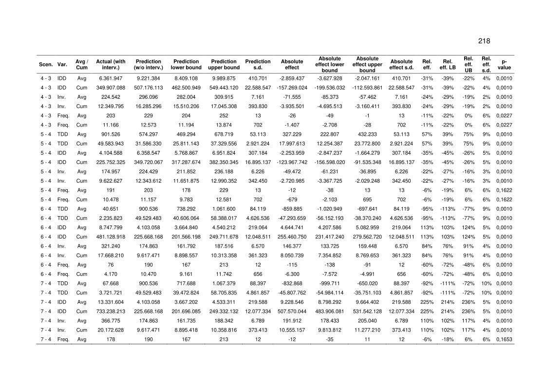
218
Scen. Var. Avg / Cum
Actual (with interv.)
Prediction (w/o interv.)
Prediction lower bound
Prediction upper bound
Prediction s.d.
Absolute effect
Absolute effect lower
bound
Absolute effect upper
bound
Absolute effect s.d.
Rel. eff.
Rel. eff. LB
Rel. eff. UB
Rel. eff. s.d.
p-value
4 - 3 IDD Avg 6.361.947 9.221.384 8.409.108 9.989.875 410.701 -2.859.437 -3.627.928 -2.047.161 410.701 -31% -39% -22% 4% 0,0010
4 - 3 IDD Cum 349.907.088 507.176.113 462.500.949 549.443.120 22.588.547 -157.269.024 -199.536.032 -112.593.861 22.588.547 -31% -39% -22% 4% 0,0010
4 - 3 Inv. Avg 224.542 296.096 282.004 309.915 7.161 -71.555 -85.373 -57.462 7.161 -24% -29% -19% 2% 0,0010
4 - 3 Inv. Cum 12.349.795 16.285.296 15.510.206 17.045.308 393.830 -3.935.501 -4.695.513 -3.160.411 393.830 -24% -29% -19% 2% 0,0010
4 - 3 Freq. Avg 203 229 204 252 13 -26 -49 -1 13 -11% -22% 0% 6% 0,0227
4 - 3 Freq. Cum 11.166 12.573 11.194 13.874 702 -1.407 -2.708 -28 702 -11% -22% 0% 6% 0,0227
5 - 4 TDD Avg 901.526 574.297 469.294 678.719 53.113 327.229 222.807 432.233 53.113 57% 39% 75% 9% 0,0010
5 - 4 TDD Cum 49.583.943 31.586.330 25.811.143 37.329.556 2.921.224 17.997.613 12.254.387 23.772.800 2.921.224 57% 39% 75% 9% 0,0010
5 - 4 IDD Avg 4.104.588 6.358.547 5.768.867 6.951.824 307.184 -2.253.959 -2.847.237 -1.664.279 307.184 -35% -45% -26% 5% 0,0010
5 - 4 IDD Cum 225.752.325 349.720.067 317.287.674 382.350.345 16.895.137 -123.967.742 -156.598.020 -91.535.348 16.895.137 -35% -45% -26% 5% 0,0010
5 - 4 Inv. Avg 174.957 224.429 211.852 236.188 6.226 -49.472 -61.231 -36.895 6.226 -22% -27% -16% 3% 0,0010
5 - 4 Inv. Cum 9.622.627 12.343.612 11.651.875 12.990.352 342.450 -2.720.985 -3.367.725 -2.029.248 342.450 -22% -27% -16% 3% 0,0010
5 - 4 Freq. Avg 191 203 178 229 13 -12 -38 13 13 -6% -19% 6% 6% 0,1622
5 - 4 Freq. Cum 10.478 11.157 9.783 12.581 702 -679 -2.103 695 702 -6% -19% 6% 6% 0,1622
6 - 4 TDD Avg 40.651 900.536 738.292 1.061.600 84.119 -859.885 -1.020.949 -697.641 84.119 -95% -113% -77% 9% 0,0010
6 - 4 TDD Cum 2.235.823 49.529.483 40.606.064 58.388.017 4.626.536 -47.293.659 -56.152.193 -38.370.240 4.626.536 -95% -113% -77% 9% 0,0010
6 - 4 IDD Avg 8.747.799 4.103.058 3.664.840 4.540.212 219.064 4.644.741 4.207.586 5.082.959 219.064 113% 103% 124% 5% 0,0010
6 - 4 IDD Cum 481.128.918 225.668.168 201.566.198 249.711.678 12.048.511 255.460.750 231.417.240 279.562.720 12.048.511 113% 103% 124% 5% 0,0010
6 - 4 Inv. Avg 321.240 174.863 161.792 187.516 6.570 146.377 133.725 159.448 6.570 84% 76% 91% 4% 0,0010
6 - 4 Inv. Cum 17.668.210 9.617.471 8.898.557 10.313.358 361.323 8.050.739 7.354.852 8.769.653 361.323 84% 76% 91% 4% 0,0010
6 - 4 Freq. Avg 76 190 167 213 12 -115 -138 -91 12 -60% -72% -48% 6% 0,0010
6 - 4 Freq. Cum 4.170 10.470 9.161 11.742 656 -6.300 -7.572 -4.991 656 -60% -72% -48% 6% 0,0010
7 - 4 TDD Avg 67.668 900.536 717.688 1.067.379 88.397 -832.868 -999.711 -650.020 88.397 -92% -111% -72% 10% 0,0010
7 - 4 TDD Cum 3.721.721 49.529.483 39.472.824 58.705.835 4.861.857 -45.807.762 -54.984.114 -35.751.103 4.861.857 -92% -111% -72% 10% 0,0010
7 - 4 IDD Avg 13.331.604 4.103.058 3.667.202 4.533.311 219.588 9.228.546 8.798.292 9.664.402 219.588 225% 214% 236% 5% 0,0010
7 - 4 IDD Cum 733.238.213 225.668.168 201.696.085 249.332.132 12.077.334 507.570.044 483.906.081 531.542.128 12.077.334 225% 214% 236% 5% 0,0010
7 - 4 Inv. Avg 366.775 174.863 161.735 188.342 6.789 191.912 178.433 205.040 6.789 110% 102% 117% 4% 0,0010
7 - 4 Inv. Cum 20.172.628 9.617.471 8.895.418 10.358.816 373.413 10.555.157 9.813.812 11.277.210 373.413 110% 102% 117% 4% 0,0010
7 - 4 Freq. Avg 178 190 167 213 12 -12 -35 11 12 -6% -18% 6% 6% 0,1653
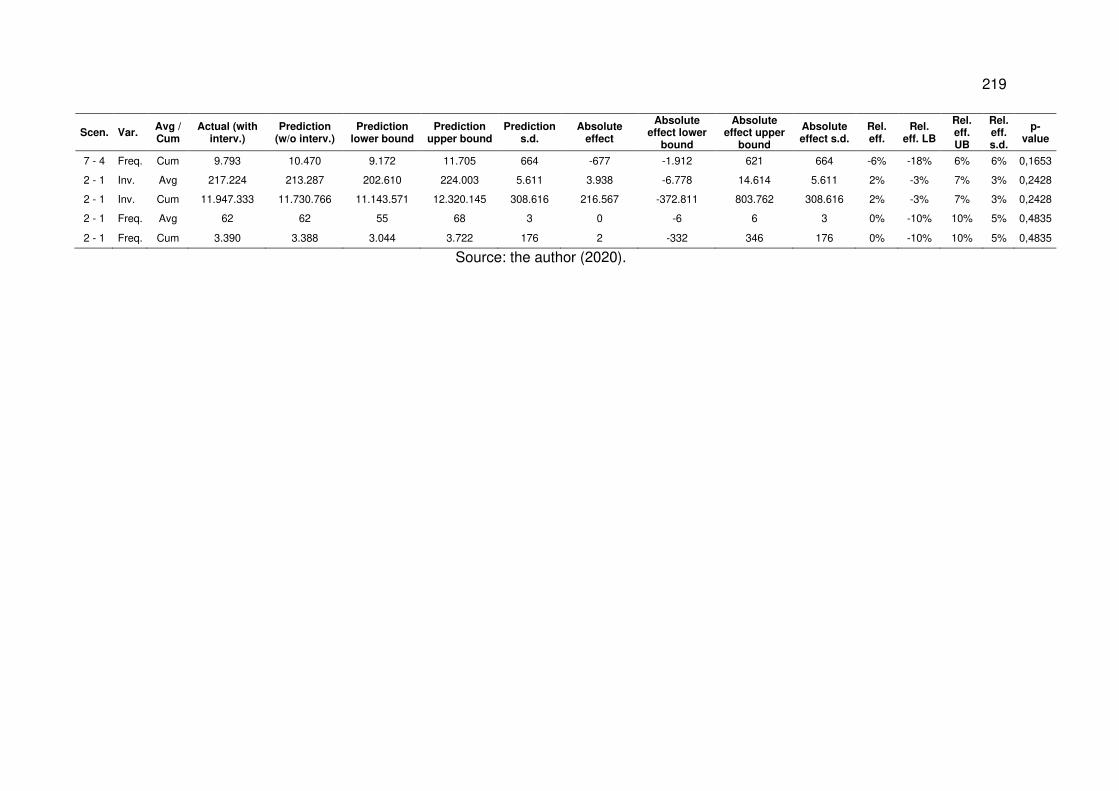
219
Scen. Var. Avg / Cum
Actual (with interv.)
Prediction (w/o interv.)
Prediction lower bound
Prediction upper bound
Prediction s.d.
Absolute effect
Absolute effect lower
bound
Absolute effect upper
bound
Absolute effect s.d.
Rel. eff.
Rel. eff. LB
Rel. eff. UB
Rel. eff. s.d.
p-value
7 - 4 Freq. Cum 9.793 10.470 9.172 11.705 664 -677 -1.912 621 664 -6% -18% 6% 6% 0,1653
2 - 1 Inv. Avg 217.224 213.287 202.610 224.003 5.611 3.938 -6.778 14.614 5.611 2% -3% 7% 3% 0,2428
2 - 1 Inv. Cum 11.947.333 11.730.766 11.143.571 12.320.145 308.616 216.567 -372.811 803.762 308.616 2% -3% 7% 3% 0,2428
2 - 1 Freq. Avg 62 62 55 68 3 0 -6 6 3 0% -10% 10% 5% 0,4835
2 - 1 Freq. Cum 3.390 3.388 3.044 3.722 176 2 -332 346 176 0% -10% 10% 5% 0,4835
Source: the author (2020).