1

Greenhouse gas emissions -

do carbon taxes work?

Annegrete Bruvoll and Bodil Merethe Larsen* Statistics Norway

Abstract

During the last decade, Norway has carried out an ambitious climate policy by implementing a

relatively high carbon tax already in 1991. The Norwegian carbon taxes are among the highest in the

world. Data for the development in CO2 emissions provide a unique opportunity to evaluate carbon

taxes as a policy tool for CO2 abatement. We combine a divisia index decomposition method and

applied general equilibrium simulations to decompose the emission changes, with and without the

carbon taxes, in the period 1990-1999. We find that despite significant price increases for some fuel-

types, the carbon tax effect on emissions was modest. The taxes contributed to a reduction in onshore

emissions of only 1.5 percent and total emissions of 2.3 percent. With zero tax, the total emissions

would have increased by 21.1 percent over the period 1990-1999, as opposed to the observed growth

of 18.7 percent. This surprisingly small effect relates to the extensive tax exemptions and relatively

inelastic demand in the sectors in which the tax is actually implemented. The tax does not work on the

levied sources, and is exempted in sectors where it could have worked.

Key words: Greenhouse gas emissions, carbon taxes, applied general equilibrium model, divisia index analysis. JEL classification: H21, O13, Q40 Address: Annegrete Bruvoll, Statistics Norway, Research Department, P.O. Box 8131 Dep. N-0033 Oslo, Norway. Telephone: +47-21 09 49 48. Telefax: +47-21 09 49 63. E-mail: Annegrete.Bruvoll@ssb.no. Bodil Merethe Larsen, Statistics Norway, Research Department, P.O. Box 8131 Dep. N-0033 Oslo, Norway. Telephone: +47-21 09 49 37. Telefax: +47-21 09 49 63. E-mail: Bodil.Merethe.Larsen@ssb.no.

* We would like to thank Torstein Bye, Brita Bye and Taran Fæhn for useful comments on previous versions of this paper.

2

1 Introduction

Emissions of greenhouse gases into the atmosphere may contribute to climate change. The recognition

of this possibility has led countries to implement tax regimes that are constructed to curb emissions.

The question of whether such tax regimes actually work or not remains unanswered empirically. In

this article, we investigate, evaluate and quantify the environmental effects of CO2 taxes in Norway.

Surprisingly, in spite of the relatively high Norwegian carbon tax rates, the effect on emissions is low.

Taxes on fossil fuels are common in most countries, but these are often introduced on fiscal grounds

rather than as instruments for reducing CO2 emissions.1 Some countries have, however, implemented

Pigouvian tax regimes to curb the emissions of climate gases, and Norway and Sweden have levied the

highest rates per ton CO2 (Ministry of Finance 1995, Ministry of Environment 2001). Within a few

years we expect that the use of price mechanisms to combat CO2 emissions will be expanded. Many

countries will participate in a quota-based emission trading system for greenhouse gases to fulfill the

Kyoto Protocol, cf. the Marrakech agreement. Thus, there is a great need for information of the

functioning of price-based incentives. The Norwegian history of carbon taxes provide researchers with

a unique opportunity to evaluate the effects of such taxes and to shed light on the possible effects of a

quota-based emission trading system for CO2.

The basis of our analysis is the observed development in greenhouse gas emissions in Norway over the

previous decade. The analysis is conducted in three steps, combining two different methods. In the

first step, we subdivide the observed changes in emissions from 1990 to 1999 into eight different

driving forces applying a divisia index decomposition method. We try to reveal the main mechanisms

behind the changes in emissions the last decade, such as production growth and changes in the

production structure and energy intensity. These observed changes have been influenced by fossil fuel

1 Optimal taxation of goods and externalities in a second best framework is discussed in Sandmo (1975).

3

price changes and carbon taxes directly and indirectly. The direct effect is energy substitution. The

indirect effects come through overall cost transfer and labor market adjustments. In the second step,

we apply a disaggregated general equilibrium model (AGE model) to quantify the isolated effect of

carbon taxes. We compare the model simulations for 1999 with and without carbon taxes and

decompose the outcome from this AGE model. In the final step we use this to calculate the tax effect

on each of the driving forces from the first step.

One might argue that the AGE model alone would be a sufficient tool in estimating the carbon tax

effects’ on emissions. However, any model of the economy will necessarily reflect a simplified picture

of the true development, and as scientists we are not able to conduct controlled experiments of the

economy. Instead, we extract information about the driving forces from the actual observed economic

development. We then estimate the tax effect on these observed forces by the means of a carbon tax

analysis in a controlled AGE model based on econometrically determined elasticities and simultaneous

behavior in complex markets.

The literature offers a range of ex ante studies of how taxes can reduce emissions and the involved

cost. Most such studies are based on simulations on computable general equilibrium models, see e.g.

Manne and Richels (1991), Jorgenson and Wilcoxen (1993) and Bye (2000). Some studies discuss a

“climate cost function”, i.e. a path showing the model correlation between different emission goals

and GDP reductions, see e.g. OECD (1992). In these analyses, calculations of energy use are made

both with and without taxes. Other studies apply a counterfactual (ex post) method, in which the level

of estimated energy consumption is adjusted (calibrated) to the level actually observed. Larsen and

Nesbakken (1997) perform a partial counterfactual study of the Norwegian CO2 taxes applying

sectoral models of the Norwegian economy. Another method used to study changes in emissions is a

divisia index decomposition analysis, see e.g. Schipper et al. (1997), Selden et al. (1999) and Bruvoll

and Medin (2002). Such ex post analyses do not quantify the causal relationship between emissions

and the environmental policy. Our analysis adds to the literature in that we consistently combine a

4

decomposition method applied on both historical observations and AGE simulations to analyze effects

of carbon taxes.

The paper is organized as follows: In section 2 we describe the development in greenhouse gas

emissions and carbon taxes in Norway. We study the changes in the main greenhouse gases over the

years 1990 to 1999 in a divisia index decomposition analysis in section 3, while we perform the AGE

simulation of the economy with and without carbon taxes in section 4. In section 5, we combine the

decomposition analysis and the AGE analysis, and estimate the carbon taxes’ effect on the observed

emission changes and each of the decomposed factors. In section 6, we discuss and conclude from the

analysis.

2 Greenhouse gas emissions and carbon taxes 1990-1999

In 1999, the total Norwegian greenhouse gas (GHG) emissions amounted to 56.0 mill. tonnes CO2,

measured in GWP equivalents.2 According to the Kyoto Protocol, Norwegian GHG emissions can

increase by one percent compared to the 1990 level by 2008-12. Over the first ten years since 1990,

the distance to the goal steadily increased. Emissions of CO2, CH4 and N2O measured in terms of

GWP increased by 15.5 percent from 1990 to 1999 (see Figure 1). Emissions of CO2, the dominant

GHG, increased by nearly 19 percent in the same period and amounted to 41.7 mill. tonnes in 1999.

This growth in GHG emissions took place despite an active climate policy, which particularly

involved taxes and imposed treatment of methane from landfills. GHG emissions per unit of GDP,

however, were reduced by 20 percent over these nine years.

In 1991, Norway introduced carbon taxes, which have later worked as the main climate policy

instrument (Ministry of Finance 1996). The taxes have steadily expanded, and in 1999 the average

2 Global Warming Potential; the accumulated climate effect of greenhouse gases measured in terms of the effect of CO2.

5

Norwegian carbon tax was about US$ 18 per tonne CO2. An optimal tax system requires a uniform tax

rate for all sources, see e.g. Hoel (1996). However, a common feature of European environmental

taxation is indeed that of extensive exemptions and differentiation of tax rates (Ekins and Speck 1999).

As we see from Table 1, this applies for Norwegian carbon taxes as well. Gasoline faces the highest

tax rate with US$ 44 per tonne CO2. The carbon tax on gasoline constituted 13 percent of the

purchaser price in 1999, while the corresponding shares for auto diesel and light fuel oils were 7 and

14 percent, respectively. A particular feature of the Norwegian economy is the importance of the

petroleum-producing sector, both with respect to economic significance and emissions consequences.

In the 1990’s 25-30 percent of total CO2 emissions in Norway came from this sector. Petroleum

production carries a relatively high burden from climate policy, as seen from Table 1 where the carbon

taxes on oil and natural gas extraction are set on a comparatively high level. The carbon taxes are

additional to several other taxes on fossil fuels, such as excise on petrol and auto fuel tax. The revenue

from these taxes comprises twice the revenue from carbon taxes. On the other hand, several industries

with relatively high emissions, such as the metal producing process industries, are partly or totally

exempted from the carbon tax. Process emissions comprise petroleum vapors and emissions from the

use of coal and coke for reduction of ores to metals, i.e. manufacturing of ferroalloy, carbide and

aluminum. There is also exemptions for fishing, air and ocean transport, manufacturing of cement and

leca and land-based use of gas. Manufacturing of pulp and paper and herring flour face half carbon

tax.

The exemption arrangements imply that the CO2 taxes cover about 64 percent of total CO2 emissions

in Norway. On average, weighted by the emissions for sources that are levied the tax and for sources

that are exempted, the carbon tax is 18 US$ per tonne CO2. To compare, Hagem and Holtsmark 2001

estimated an international quota price based on free international competition in the permit market to

as low as 5 US$ per tonne CO2.

6

Figure 1. GHG emissions in Norway 1990–1999, 1990=1. Sum of weighed global warming

potential (GWP) for CO2, CH4 and N2O 1)

0.80

0.85

0.90

0.95

1.00

1.05

1.10

1.15

1.20

1990 1991 1992 1993 1994 1995 1996 1997 1998 1999*

CO2

CH4

N2O

Sum

1) GWP: CO2= 1, CH4=21, N2O= 310.

* Preliminary figures.

Table 1. Carbon taxation in Norway, 1999. US$ * per tonne CO2

US$ per tonne

Maximum taxes by fuels:

Gasoline 44.1 Coal for energy purposes 21.0 Auto diesel and light fuel oils 19.2 Heavy fuel oils 16.4 Coke for energy purposes 16.0

Taxes by sectors and fuels: North Sea petroleum extraction - Oil extraction 37.2 - Natural gas extraction 42.3 Pulp and paper industry, herring flour industry - Light fuel oils, transport oils (gasoline, diesel etc.) 9.6 - Heavy fuel oils 8.2 Ferro alloys-, carbide- and aluminum industry - Coal and coke for processing 0.0 Land-based use not covered by the petroleum tax legislation - Gas 0.0 Cement and leca production 0.0 Air transport 0.0 Foreign carriage, fishing and catching by sea 0.0 Domestic fishing and goods traffic by sea 0.0 Average tax for all sources 18.2

* 1 USD ≅ 9.0 NOK

Source: Statistics Norway

7

3 Decomposition of greenhouse gas emissions

To isolate the driving forces behind the changes in GHG emissions over the period 1990 to 1999, we

apply a divisia index approach as described in Bruvoll and Medin (2002).3 We separate stationary and

mobile emissions (energy related emissions) from process emissions. We further decompose the

development in emissions into eight different driving forces; population growth, growth in per capita

GDP, structural changes, energy and material intensity, energy mix and other changes specific to

energy and process related emissions.

To illustrate the decomposition procedure, total emissions from stationary and mobile combustion

(PSM) and processes (PPR) in a given year can be formulated as:

(1) ∑∑≡

i j

j

j

j

j

ij

ij

SMijSM

BB

Y

Y

Y

Y

E

E

E

E

PP , and

(2) BB

Y

Y

Y

Y

M

M

PP

j

j

j

j j

PR

jPR

∑≡ ,

where E is energy use (measured in PJ), M is the use of material input, Y is total production (GDP), B

is population, i is energy type and j is sector. Yj is output in sector j and total consumption for the

household sector, all in fixed 1990 prices. When we investigate the changes in emissions from 1990 to

1999, we compute the contribution from changes in the components, see Appendix 1 for a description.

The equations (1) and (2) show that we decompose emission changes into components that reveal the

effect of population growth (B), per capita GDP growth (Y/B) and production structure changes (Yj/Y).

3 Selden et al. (1999) decompose the changes in US air emissions from 1970-1990 into the effects from changes in GDP,

production structure, energy intensity and energy mix. Bruvoll and Medin (2002) isolate the driving forces into the same

categories, adding the effect of population growth and changes in the combustion method, in an analysis of changes in 10

environmentally damaging emissions in Norway over the period 1980-1996.

8

We further decompose the energy related emissions per produced unit within each sector into changes

in energy intensity (Ej/Yj), energy mix (Eij/Ej) and a factor capturing changes in emissions per energy

unit within each sector (PSMij/Eij). The process related emissions per produced unit are decomposed

into changes in the material intensity (Mj/Yj) and a factor capturing changes in emissions per unit of

material input (PPRj/Mj).

The carbon tax influences most of these components. The actual differentiated CO2 taxes in Norway

tend to circumvent the composition of sectors and the mix of energy types and intermediates that an

optimal tax regime would create. A tax on carbon intensive materials also influences the energy and

material intensity. In general, additional costs tend to decrease total production. We will now

decompose the actual observed emission changes. These changes include the carbon tax effect, and we

will estimate the separate carbon tax effect in section 5.

Our analysis covers emissions of CO2, CH4 and N2O from all sources and sectors in the Norwegian

economy.4 The economy is divided into 8 sectors5 and 18 energy types. The low level of emissions from

the combustion of energy originate from the fact that most of the heating in Norway is based on

electricity. There are no emissions related to the production of electricity, since it is based on

hydropower. Thus, electricity is not included in this analysis. Data on emissions to air, energy use and

production are documented in the Emissions accounts and the National accounts of Statistics Norway

(see e.g. Statistics Norway 1997 and Rypdal 1993).

Table 2 displays the contribution to emission changes from the different components for each of the

greenhouse gases and for the gases weighed in terms of GWP. The factoring is complete, and the

4 Due to the international standard for emissions calculations, ocean and air transport outside the Norwegian border are not

accounted for. 5 Private households, private services, government services, energy producers, energy-intensive manufacturing, manufacture

of pulp and paper, other manufacture and mining and other industries.

9

components add up to total changes in emissions according to the applied decomposition method. As

we see from Table 2, the main driving forces counteracting the emission increasing tendency

following economic growth, is reduced energy intensity, changes in the energy mix and reduction in

the emissions / material input ratio. We will now discuss each of the components in detail.

Table 2. Changes in emissions from 1990 to 1999 and the contribution from each component.

Percent

Components CO2 CH4 N2O Weighted

total 1)

Population 5.0 5.0 5.0 5.0

Scale 30.4 30.4 30.4 30.4

Composition of sectors 2.9 -0.7 -17.7 0.1

Energy intensity -10.7 -1.3 -0.6 -8.2

Energy mix -3.3 0.3 0.3 -2.4

Other technique, energy 0.0 -0.1 6.1 0.7

Material intensity -1.2 -2.2 -3.8 -1.6

Other technique, process -4.5 -23.3 -17.0 -8.5

Total change 18.7 8.2 2.8 15.5

1) Total is weighted by GWP: CO2= 1, CH4=21, N2O= 310.

The population component contributed to a 5 percent growth in the greenhouse gases, keeping all the

other components, i.e. emissions per capita, constant. The scale component (the growth in GDP per

capita) is 30 percent. These two components add up to a total GDP growth of 35 percent. This means

that assuming constant energy intensity, energy mix, production structure, and all the other factors

influencing the relationship between production and emissions constant, the GDP growth would imply

a growth in total greenhouse gas emissions of 35 percent over the period 1990 to 1999.

Changes in the composition of sectors contributed to increased emissions of CO2, but to reductions in

the emissions of CH4 and N2O, see Table 2 and Figure 2. The higher than average growth in energy

producing sectors, in combination with the relatively large share of CO2 emissions of 27 percent in

1990, contributed to increased emissions of CO2. We find the same effect in metal production, which

10

contributed to 15 percent of the emissions.6 As noted before, this decomposition analysis alone does

not analyze the tax effect. However, it is interesting to note that the high increase in energy production

took place despite the relatively high carbon tax levied on oil extraction, and that process emissions

from metal production are exempted from the carbon tax (see Table 1). The emission increasing effect

for CO2 was somewhat modified by a lower than GDP growth in private consumption and the

production of private services.

Figure 2. Production and growth in production, 1990 - 1999. Mill. NOK and percent

0

100

200

300

400

500

600

En

erg

y p

rod

uce

rs

Oth

er

ind

ustr

ies

Go

ve

rnm

en

t

se

rvic

es

Oth

er

ma

nu

factu

rin

g

an

d m

inin

g

Priva

te h

ou

se

ho

lds'

co

nsu

mp

tio

n

En

erg

y-i

nte

nsiv

e

ma

nu

factu

rin

g

Priva

te s

erv

ice

s

Ma

nu

factu

re o

f p

ulp

an

d p

ap

er

pro

du

cts

0

10

20

30

40

50

60

1990

1999

Growth in per cent

Per cent

In 1990, CH4 was mainly generated in government services (public waste treatment facilities) and

other industries (agriculture), and N2O in energy-intensive manufacturing and other industries

(agriculture). The production growth in these sectors was close to the growth in GDP, thus changes in

the production structure had marginal effect on these emissions. The negative composition component

for N2O is mainly due to reduced production in the agricultural sector, which generates about half of

the total emissions of N2O.7

6 The growth in metal production from 1990 to 1999 was 43 percent. In our model, metal production is included in the sector

energy-intensive manufacturing. To include this structural effect, we have separated metal production as an own sector for

the calculation of CO2. 7 In our model, agriculture is included in the sector other industries. As for metal production and CO2 emissions we have

calculated the effect of the agricultural sector separately for N2O.

11

Energy intensity reduction is most important for explaining the slowdown of the emissions, and for

CO2 in particular. Except for the sectors producing pulp and paper products and to some degree other

industries, total energy use in relation to total production was reduced over the years 1990 to 1999 (see

Figure 3). On average, the energy intensity was reduced by 7.2 percent from 1990 to 1999. Note that

the energy intensity changes only relate to fossil fuels, since non-polluting electricity consumption is

not included in the analysis. The Norwegian energy supply system departs from most other countries

in that the economy relies heavily on electricity consumption (electricity as share of total energy

consumption amount to 20-25 percent in the period). Thus, the average reduction in total energy

intensity may depart from the changes in the energy intensity related to fossil fuels.

Figure 3. Change in energy intensity from 1990 to 1999. Percent

- 3 5

- 3 0

- 2 5

- 2 0

- 1 5

- 1 0

- 5

0

5

1 0

Energ

y p

roducers

Oth

er

industr

ies

Govern

ment

serv

ices

Oth

er

manufa

ctu

ring

and m

inin

g

Private

household

s

Energ

y-inte

nsiv

e

manufa

ctu

ring

Private

serv

ices

Manufa

ctu

re o

f pulp

and p

aper

pro

ducts

Tota

l

The energy intensity effect on CO2 emissions is a reduction of 11 percent. With a 30 percent reduction

in energy intensity and a significant share of the emissions, private households contributed

significantly (-7 out of the -11 percent) to the negative energy intensity component. The main reason is

more efficient use of gasoline, which originates from improved technology of imported cars. This

technological change cannot be ascribed to the Norwegian climate policy, since Norway does not have

an own car industry. However, the price of gasoline might influence the consumers' choice of vehicle

technology. The energy intensity reduction was rather modest for energy producers, but due to their

significant emissions, their contribution to the energy intensity component amounted to -2 of 11

percent.

12

The role of the reduced energy intensity for CO2 emissions is a continued trend from the development

in CO2 emissions the latest 20 years. Torvanger (1991) found that lower energy intensity was the main

reason for reduced CO2 emissions per unit produced in OECD over the period 1973-87. Also, Sun

(1999) points to the importance of energy intensity, as he argues that an inverted U-shaped curve

between income and CO2 emissions for a range of countries merely reflects an inverted U-shaped

relationship between income and energy intensity.

The smaller effect of energy intensity changes on CH4 and N2O is not surprising, as 96 and 94 percent

of these emissions, respectively, originate from other processes than burning of fossil fuels.

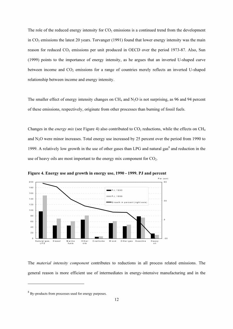
Changes in the energy mix (see Figure 4) also contributed to CO2 reductions, while the effects on CH4

and N2O were minor increases. Total energy use increased by 25 percent over the period from 1990 to

1999. A relatively low growth in the use of other gases than LPG and natural gas8 and reduction in the

use of heavy oils are most important to the energy mix component for CO2.

Figure 4. Energy use and growth in energy use, 1990 - 1999. PJ and percent

0

2 0

4 0

6 0

8 0

1 0 0

1 2 0

1 4 0

1 6 0

1 8 0

2 0 0

N a tu r a l g a s ,

L P G

D ie s e l M a r in e

f u e ls

O th e r

o i ls

C o a l / c o k e W o o d O th e r g a s G a s o l in e H e a v y

o i l

- 3 0

0

3 0

6 0

P J , 1 9 9 0

P J , 1 9 9 9

G r o w th in p e r c e n t ( r ig h t a x is )

P e r c e n t

The material intensity component contributes to reductions in all process related emissions. The

general reason is more efficient use of intermediates in energy-intensive manufacturing and in the

8 By-products from processes used for energy purposes.

13

energy sectors, while less input relative to output in the agricultural sector is particularly important to

CH4 and N2O.

The other technique component for energy (material) related emissions captures factors that change

the emission / energy (material) ratio, such as the effect of emission abatement and technological

changes that are not included in the other components.

The other technique component for process related emissions is the most important component for

methane and N2O, and in total the most important factor counteracting economic growth. Although

methane emissions from landfills increased over the period, the emissions within the methane

generating sectors per unit of material input decreased. The reason is landfill gas treatment and less

waste for landfill. The effect on N2O is due to lower emissions per unit of material use in the

agricultural sector and in the production of fertilizers. This component also contributes to lower CO2

emissions. This is mainly due to changes in the production processes, which led to a decrease in the

process related CO2 emissions per total material input, and particularly in energy-intensive

manufacturing.

A negative side effect of the use of catalytic converters in automobiles is an increase in N2O

emissions. Thus, the other technique component for energy related emissions contributed to increased

N2O emissions. This component is zero for CO2 emissions, since the CO2 emissions per energy unit is

constant for fossil fuels.

4 The AGE analysis

In order to estimate the carbon taxes’ effect on each of the decomposed observed emission changes (in

Table 2), we simulate the Norwegian economy with and without carbon taxes in an AGE analysis. A

carbon tax will affect the economy through several mechanisms, such as changes in fossil fuel and

14

other product prices, production and consumption. In contrast to a partial equilibrium analysis, in

principle this general equilibrium analysis will capture all spillover effects, and in equilibrium

simulate the total effects of carbon taxes on the economy.

The applied AGE model of the Norwegian economy, MSG-6, is an integrated economy and emission

model, designed for studies of economic and environmental impacts of climate policy.9 A

documentation of the model is provided in Holmøy et al. (1999), Bye (2000) and Fæhn and Holmøy

(2000). Previous ex ante analyses of carbon tax policies concerned with effects of future stabilization

of CO2 emissions are given in Glomsrød et al. (1992), Brendemoen and Vennemo (1994) and Aasness

et al. (1996), while Bye (2000) and Bye and Nyborg (1999) analyze welfare effects of different carbon

tax reforms using a dynamic version of the CGE model utilized here.

MSG-6 gives a detailed representation of the Norwegian economy. The model specifies 60

commodities and 40 industries, classified particularly to capture important substitution possibilities

with environmental implications. The sectors’ energy demand varies, both with respect to the energy

intensity, and the possibility for substitution between energy types, and between energy and other

input.

Closure rules are restrictions in the model that “determine” variables that are endogenous in the

economy but unexplained by the model. In the model version used in this project, the current public

use of resources and taxes are exogenous, whereas the tax bases are endogenous. We assume that the

fixed development of public budgets is maintained when carbon taxes increase, i.e. the public budget

constraint is exogenous. This is obtained by lump sum income transfers to households. The current

account and labor supply are exogenous. The base year is 1992, which means that the model is

calibrated to the 1992 National Accounts. Appendix 2 offers a more detailed description of the model.

9 MSG-6 is an acronym for Multi Sectoral Growth - version 6. Various versions of the MSG model have been used in

Norwegian long-term planning for many years.

15

4.1 The zero-tax and tax scenarios

We create a zero-tax scenario by subtracting the CO2 tax from the total indirect taxes of each of the

fossil fuels and then simulating the model. By comparing the zero-tax scenario with a scenario in

which the actual CO2 taxes are implemented, we quantify the carbon tax effect on economic variables

and emissions.

In the zero-tax scenario, we have implemented numerical values for total indirect taxes exclusive of

CO2 taxes for the year 1999 and simulated the model for the period 1992-99. The long-term model

needs some years to reach the new equilibrium. To attain equilibrium in our year of observation, 1999,

we have implemented the actual CO2 taxes for 1999 over the entire period 1993-99. In 1999, the CO2

taxes’ share of total taxes (exclusive of VAT) was 18 percent for petrol, 16 percent for transport

mineral oil (auto diesel and marine gas oils) and 78 percent for mineral oil for heating (light and heavy

fuel oils). In the reference scenario, the variable values of the base year 1992 are in accordance with

the actual (the National Accounts). This is not (necessarily) the case for the other years of the

reference scenario. However, we are interested in the relative changes between the two scenarios, thus

the actual values of the variables in the reference scenario are of less importance. Except for the

carbon tax, all exogenous variables are constant between the two scenarios.

The Norwegian extraction of oil is highly influenced by political decisions, and CO2 taxes will have

small or no influence on oil production. Since we analyze a national CO2 tax, it is reasonable to

assume that the effect on the crude oil price is negligible. Thus, the MSG-6 model treats the petroleum

production as exogenous. Studies indicate, however, that there has been a shift to more energy-

efficient equipment on the oil platforms as a result of the CO2 tax. ECON (1997) estimate a CO2 tax

effect of 3 percent on offshore CO2 emissions. We incorporate this in the analysis in section 5.

16

4.2 General AGE effects of the carbon tax

A direct effect of the CO2 tax is that households and production sectors will substitute some of their

fossil fuel consumption for electricity.10 The fossil fuel intensity of the economy and hence emissions

will decrease (see the nested tree production technology and the utility tree in Appendix 2 and

elasticities of substitution in Table 3). Changes in the CO2 tax will also influence total energy

consumption through substitution against other inputs. Due to different substitution elasticities

between electricity and oil, the switch from using oil to using electricity varies between the sectors.

The demand for energy for stationary purposes is a CES aggregate of electricity and fuel oil. Table 3

gives an overview over the econometric estimates of the elasiticities of substitution. We can see, e.g.

that the effect of a change in relative prices of electricity and fuel oil on the factor relationship

between electricity and oil is high in the pulp and paper sector and zero in the metal sector.11

The substitution from fossil fuels does not prevent increases in the unit price of energy and in the

service price of energy-using machinery etc., see Figure A2 in Appendix 2. The cost increase is higher

the higher the fossil fuel intensity of the sector, and leads to substitution- and scale effects in the fossil

fuel demand of the firms. Reduced production, especially in the fossil fuel intensive industries,

transmits to other industries through deliveries of real capital and material inputs. Price increases for

domestically produced inputs will modify the first-order substitution effects of fossil fuel. Machinery

becomes more expensive to produce, which reduces the incentive to choose less energy intensive

machinery and increases the incentive to substitute labor for machinery which use energy. The

adjustments of inputs and production ensure equilibrium in the product markets. The labor market and

the current account are cleared through changes in wages and household consumption.

10 Nearly 100 percent of the Norwegian electricity production is covered by hydropower.

11 See Alfsen et al. (1996) for a documentation of the econometric model and elasticities of substitution implemented in

MSG.

17

Table 3. Elasticites of substitution in MSG-61)

Sector

Electricity

vs.

heating oils

Machinery

vs. energy

Non-polluting

transport2)

vs. polluting

transport

Transport oils vs.

transport equipment,

own transport vs.

polluting

commercial

transport

Gasoline

vs. user

cost of cars

Private

transport

vs. traditional

public transport

Agriculture -0.28 -0.38 -0.50 0.00

Manufacture of various

consumption goods -0.23 -0.33 -0.50 0.00

Manufacture of wood

products, chemical and

mineral products, printing

and publishing -0.90 -0.68 -0.50 0.00

Manufacture of pulp and

paper articles -1.34 -0.33 -0.50 0.00

Manufacture of industrial

chemicals (incl. cement and

leca3)) -0.25 -0.46 -0.50 0.00

Manufacture of metals (incl.

coal and coke for

processing3)) 0.00 -0.62 -0.50 0.00

Manufacture of metal

products, machinery and

equipment -0.29 -0.46 -0.50 0.00

Manufacture of ships and

oil production platforms 0.00 -0.56 -0.50 0.00

Wholesale and retail trade -0.37 -0.70 -0.50 0.00

Government production

sectors -0.18 0.00 0.00 0.00

Production of other private

services -0.18 -0.91 -0.50 0.00

Other sectors (incl. herring

flour industry, fishing, air

and sea transport3)) 0.00 0.00 -0.50 0.00

Household sector -0.80 -0.20 -1.20

1) MSG-6 specifies 40 production sectors. In this table we have aggregated sectors in which the implemented elasticities of substitution are

equal.

2) Railway, post and telecommunication.

3) See Table 1 for a comparison with the carbon tax system.

As a result of the CO2 taxes GDP is reduced by 0.06 percent and total household consumption by 0.1

percent, see Table 4. To clear the labor market, wages decrease by 0.2 percent. The households’

consumption of gasoline and heating oils decrease by 4.2 and 6.2 percent due to a price increase of 7.6

and 17.0 percent for the households’ use of these fuels. Consumption of public transport and

electricity increase due to the substitution effects. Production is reduced by 0.1 - 0.8 percent in the

industrial sectors and for some services sectors, while public transport such as air transport, railway

18

and tramway transport increase due to the households’ substitution of own transport for public

transport.

Table 4. The carbon tax effect; comparing the tax scenario and the zero-tax scenario in 1999.

Percent

Percent difference

GDP -0.06

Total household consumption -0.10

consumption of gasoline -4.2

consumption of heating oils -6.2

consumption of public transport 0.6 to 1.9

consumption of electricity 0.5

Production in industrial sectors -0.1 to -0.8

Production in public transport 0.4 to 1.2

Wages -0.2

5 The tax effect on CO2 emissions

We will now decompose the simulated CO2 emissions for 1999 in order to analyze the effect of the

carbon taxes on each of the factors in the decomposed observed CO2 emissions in section 3. The

economy in the AGE decomposition is divided into 40 sectors and fossil fuels is disaggregated into

three types.12

The effect on onshore emissions, as estimated by use of MSG-6, is a reduction of 1.47 percent. As

explained in the previous section, the offshore sector is treated exogenously in the model. Based on

evaluations of the carbon tax in the offshore sector (ECON 1997), we have reduced the offshore

energy and material intensity, and hence emissions, by 3.0 percent. Altogether, this yields a reduction

in total national CO2 emissions of 2.32 percent as a result of the carbon tax.

The decomposition analysis of the observed data in section 2 provides us with valuable information on

the driving forces behind the emission changes that has actually been in work. However, that analysis

12 Gasoline, mineral oil for transportation (auto diesel and marine gas oil) and mineral oil for heating (light and heavy fuel

oils).

19

gives no information on the impact of the most heavily emphasized GHG policy, namely the carbon

tax. In order to isolate the effects of the carbon tax, we first decompose the results from the AGE

simulations. This decomposition enables us to estimate the tax effect on each of the components from

the observed data from section 2. The final result is zero-tax estimates on the decomposed emission

changes from 1990 to 1999. Table 5 shows the results.

Table 5. Decomposition of observed changes in emissions and of the AGE scenarios in 1999.

Percent change in CO2 emissions

Component

Observed emission

changes,

1990-1999

The AGE analysis.

Difference tax

scenario and zero-tax

scenario, 1999

Estimated emission

changes

with zero carbon tax,

1990-1999

Population 5.01 0.00 5.01

Scale 30.41 -0.06 30.46

Composition of sectors 2.89 -0.01 2.89

Energy intensity -10.67 -1.73 -8.94

Energy mix -3.27 -0.54 -2.73

Material intensity (process) -1.17 0.00 -1.17

Other technique (process) -4.47 0.01 -4.48

Total change in CO2 emissions 18.73 -2.32 21.05

The observed CO2 emissions amounted to 41.7 mill. tonnes in 1999. Combining the observed data

with the AGE tax analysis, we find that the observed emissions is 2.32 percent lower than what the

emissions would have been without the carbon tax. Combining the AGE analysis with the observed

data, we estimate the zero-tax CO2 emissions in 1999 to 42.7 mill. tonnes. This implies that the growth

in emissions from 1990 to 1999 without the tax would have been higher; 21.05 percent over the period

1990-1999, as opposed to observed growth of 18.73 percent (see the last row of Table 5).

The second column in Table 5 corresponds to the decomposition performed in section 3 (see Table 2).

The third column of Table 5 shows the decomposed carbon tax effect as simulated by use of the AGE

model (including the exogenous changes in the offshore sector) as described in section 4. The carbon

tax has particularly influenced the use of energy. Reduced energy intensity and changes in the

composition of energy contributed to emission reductions of 1.73 percentage points and 0.54

percentage points, respectively, of the totally 2.32 percent reduction due to the carbon tax. The tax has

20

also slowed down the economic growth (the scale effect) to some extent. The carbon tax reduced GDP

and hence the emissions by 0.06 percent.

The fourth column displays the estimated components net of tax effects. We see that the estimated

energy intensity component if no carbon tax was implemented in Norway is -8.94 percent, 1.73

percentage points lower than the component calculated on the basis of observed data. The second most

important effect of the tax is the influence on the energy mix, which without the tax would have

contributed to an emission reduction of 2.73 percent over the period 1990 to 1999, instead of the

observed 3.27 percent.

The main reason for the tax effect on energy intensity is more efficient turbines in oil production,

which alone contributes to half of the energy intensity effect. The substitution elasticities in the

production sectors and in consumption are of vital importance to the effect on energy intensity. The

energy use in households and most of the production sectors becomes less fossil fuel intensive, and as

we can see from Table 3, the possibilities to substitute from fossil fuels to electricity in the

households, and to other inputs (especially machinery) in the production sectors, are relatively high.

Also, the emissions are relatively high in these sectors, and the tax most effectively reduces the energy

intensity in households, manufacturing of chemical and mineral products and pulp and paper products.

However, as we can see from Table 3, the households’ possibility to reduce the energy intensity

through substituting new cars for gasoline is limited. The substitution possibilities and emissions are

also relatively high in manufacturing of industrial chemicals, wholesale and retail trade and production

of other private services. The tax also affects the emissions through the reduction in energy intensity in

these sectors.

Due to the tax, households substitute electricity for fossil fuels for heating, and the household sector

contributes most to the energy mix component. Manufacturing of chemical and mineral products,

industrial chemicals and pulp and paper products and production of other private services also

21

contribute to the energy mix component. In these sectors the elasticity of substitution between

electricity and heating oils are relatively high.

The sector composition component was slightly influenced by the tax, mainly due to reduced

production in petroleum refining. The tax contributed to increase the production of air transport

services, which pulled in the direction of a positive composition component. Since air transport is

exempted from the tax, households substitute air transport for other types of transport.

Assumptions regarding closing of the model and implementation of the carbon taxes in the model

simulations will affect our results. Sensitivity analyses regarding these assumptions are a subject for

future research. For example, the carbon tax revenue could be rebated through cuts in the payroll tax

rate instead of lump sum transfers to households. We have also assumed no additional technological

change following the carbon tax, except for in the petroleum sector. This means that we may have

underestimated the carbon tax effect on emissions (see Goulder and Schneider 1999 and Zwaan et al.

2002 for analyses of technological change in climate change modeling).

6 Discussion and conclusion

In wake of the Brundtland commission (United Nations 1987), Norway has been one of the most

devoted advocates for more ambitious climate policies. A carbon tax was implemented in 1991, and

has received broad attention in the policy debate. The highest carbon tax rate of the Norwegian

economy is 44 US$ per tonne CO2. This is among the highest carbon taxes in the world and three to

four times higher than the most common estimates of the quota price in the Kyoto Protocol. Our study

shows that despite the politically ambitious carbon tax, this policy measure has had only a modest

influence on greenhouse gas emissions.

22

The Norwegian emissions of CO2 increased by 19 percent from 1990 to 1999. This growth is

significantly lower than the GDP growth of 35 percent. In other words, average emissions per unit

GDP was reduced by 16 percent over the period. We find that the most important reduction factors are

more efficient use of energy and a substitution towards less carbon intensive energy. The energy

intensity and energy mix components contributed to a reduction in CO2 emissions over the period by

14 percent. The effect of carbon taxes on these emission-reducing components has been small. The

model simulations indicate that the carbon tax contributed to a reduction in emissions of 2.3 percent.

Also, the effect of the carbon taxes in Norway is strongly dominated by the Norwegian oil and gas

sector. If we consider onshore emissions only, the carbon tax effect on emissions is reduced from 2.3

to 1.5 percent.

In light of the belief that the carbon tax has been both considerable and pioneering, these results might

seem surprising. The small effects are partly related to the exemption from the carbon tax for a broad

range of fossil fuel intensive industries, exemptions which have been principally motivated by concern

about competitiveness. The industries, in which we expect the carbon tax to be most efficient in terms

of downscaling of the production and reduced emissions, are the same industries which are exempted

from the carbon tax. The zero-tax industries consist mainly of the process industry, which explains

why there is a close to zero effect of the tax on process related CO2 emissions. If the metal sector and

industrial chemicals had not been exempted from the carbon tax, a large share of these sectors would

have proven unprofitable (Bye and Nyborg 1999). Likewise, the low possibilities to substitute from

heating oil for fishing and sea transport indicate that a tax would have reduced the production level in

these industries. Manufacture of pulp and paper faces a reduced tax rate, but can substitute to

electricity and machinery. A higher tax would probably both have reduced the emissions through the

energy mix and energy intensity.

In contrast, gasoline is levied a considerable tax that constitutes 13 percent of the price. But since the

substitution possibilities are low for transportation, the tax effect on emissions is small despite its

23

relative price importance. The households’ possibility to reduce the energy intensity through

substituting new cars for gasoline is limited. Basically, we may conclude that the tax does not work for

the sources in which it is levied, and is exempted for the sources where it would have worked.

When we consider the emissions of all greenhouse gases, policy measures aimed at reducing other

greenhouse gas emissions than CO2 seem to have been more efficient than the carbon taxes’ effect on

CO2 emissions. For example, abatement of landfill gases, and regulations of the process industries

have significantly slowed down or reduced the emissions of methane, N2O and SF6 (Ministry of

Environment 2001). Not only have these direct regulations proven far more successful, but they have

also been carried out at significantly lower costs per tonne CO2 (Bruvoll and Bye 1998). The

Norwegian carbon taxes are high, but the emissions effect is low. This implies a high cost of reducing

emissions from sources on which the tax is levied.

For countries that consider implementing a carbon tax and in future Norwegian carbon tax policy, we

recommend a more broad based, cost efficient tax, which is uniform for all sources and greenhouse

gases. With a more uniform distribution of the tax burden, it is possible to accomplish larger

reductions in the greenhouse gas emissions at lower costs. A joint international cooperation regarding

the carbon taxes would also reduce the concern related to trade effects of the domestic tax burden, and

hence ease the pressure towards tax exemptions for e.g. the process industries.

24

References

Alfsen, K.H, T. Bye and E. Holmøy, eds. (1996): MSG-EE: An Applied General Equilibrium Model

for Energy and Environmental Analyses, Social and Economic Studies 96, Statistics Norway.

Brendemoen, A. and H. Vennemo (1994): A Climate Treaty and the Norwegian Economy: A CGE

Assessment, Energy Journal 15(1), 77-93.

Bruvoll, A. and H. Medin (2002): Factors behind the environmental Kuznets curve - a decomposition

of the changes in air pollution, forthcoming in Environmental and Resource Economics.

Bruvoll, A. and T. Bye (1998): Methane emissions and permit prices for greenhouse gases, Economic

Survey 4, 31 - 40, Statistics Norway.

Bye, B. (2000): Environmental Tax Reform and Producer Foresight: An Intertemporal Computable

General Equilibrium Analysis, Journal of Policy Modelling 22(6), 719-52.

Bye, B. og K. Nyborg (1999): The Welfare Effects of Carbon Policies: Grandfathered Quotas versus

Differentiated Taxes, Discussion Papers 261, Statistics Norway.

ECON (1997): Effects of a CO2 tax on CO2 emissions from the Norwegian petroleum extraction.

ECON Report No. 50/97, Oslo. (In Norwegian)

Ekins, P. and S. Speck (1999): Competitiveness and exemptions from environmental taxes in Europe,

Environmental and Resource Economics 13, 369-396.

Fæhn, T and E. Holmøy (2000): Welfare Effects of Trade Liberalization in Distorted Economies: A

Dynamic General Equilibrium Assessment for Norway, in Harrison, G.W., S.E. Hougaard Jensen, L.

25

Haagen Pedersen and T.R. Rutherford (eds): Using Dynamic General Equilibrium Models for Policy

Analyses, North-Holland.

Glomsrød, S., H. Vennemo and T. Johnsen (1992): Stabilization of Emissions of CO2: A Computable

General Equilibrium Assessment, Scandinavian Journal of Economics 94(1), 53-69.

Goulder, L.H. and S.H. Schneider (1999): Induced technological change and the attractiveness of CO2

abatement policies, Resource and Energy Economics 21, 211-253.

Hagem, C. and B. Holtsmark (2001): From small to insignificant: Climate impact of the Kyoto

protocol with and without US, CICERO Policy Note 2001:1, http://www.cicero.uio.no.

Hoel, M. (1996): Should a carbon tax be differentiated across sectors?, Journal of Public Economics

59(1), 17-32.

Holmøy, E., B. Strøm and T. Åvitsland (1999): Empirical characteristics of a static version of the

MSG-6 model, Documents 99/1, Statistics Norway.

Jorgenson, D.W. and P.J. Wilcoxen (1993): Reducing U.S. Carbon Dioxide Emissions: An

Assessment of Different Instruments, Journal of Policy Modelling 15(5-6), 491-520.

Larsen, B.M. and R. Nesbakken (1997): “Norwegian Emissions of CO2 1987-1994. A study of some

effects of the CO2 tax”, Environmental and Resource Economics 9(3), 275-290.

Manne, A. and R.G. Richels (1991): Global CO2 Emission Reductions: The Impact of Rising Energy

Costs, Energy Journal 12(1), 87-107.

26

Ministry of Environment (2001): Norwegian climate policy, Report to the Storting no. 54 (2000-

2001). (In Norwegian)

Ministry of Finance (1996): Policies for a better environment and high employment. An English

summary of the Norwegian Green Tax Commission, Ministry of Finance, Norway.

OECD (1992): Costs of Reducing CO2 Emissions. Evidence from Six Global Models, Economics and

Statistics Working Papers, OECD.

Rypdal, K. (1993): Anthropogenic emissions of the greenhouse gases CO2, CH4 and N2O in Norway,

Reports 93/24, Statistics Norway.

Sandmo, A. (1975): Optimal taxation in the presence of externalities, Swedish Journal of Economics

77, 86-98.

Schipper, L., M. Ting, M. Khrushch and W. Golove (1997): The evolution of carbon dioxide

emissions from energy use in industrialized countries: An end-use analysis, Energy Policy 25(7-9),

651-72.

Selden, T.M., A.S. Forrest and J.E. Lockhart (1999): Analyzing the reductions in US air pollution

emissions: 1970 to 1990, Land Economics 75(1), 1-21.

Statistics Norway (1997): National accounts 1978-1996, Official Statistics of Norway C 426.

Sun, J.W. (1999): The nature of CO2 emission Kuznets curve, Energy Policy 27, 691-94.

27

Torvanger, A. (1991): Manufacturing sector carbon dioxide emissions in nine OECD countries, 1973-

87, Energy Economics 13, 168-86.

United Nations (1987): Our common future. World Commission on Environment and Development,

Oxford: Oxford University Press.

Zwaan, B.C.C., R. Gerlagh, G. Klaassen and L. Schrattenholzer (2002): Endogenous technological

change in climate change modelling, Energy Economics 24, 1-19.

Aasness, J., T. Bye and H.T. Mysen (1996): Welfare Effects of Emission Taxes in Norway, Energy

Economics 18(4), 335-346.

28

Appendix 1. Computing the emission components

The population component, N:

(1)

−= 1

0

1

0B

BPN , 100

0P

NN =

The scale component, S:

(2)

−=

0

1

0

1

0B

B

Y

YPS , 100

0P

SS =

The composition component, C:

(3)

−=∑

0

1

0

1

0Y

Y

Y

YPC

j

j

j

j , 100

0P

CC =

The energy intensity component, H:

(4)

−=∑

0

1

0

1

0

j

j

j

j

j

SM

jY

Y

E

EPH , 100

0P

HH =

The energy mix component, M:

(5) ∑∑

−=

j j

j

ij

ij

i

SM

ijE

E

E

EPZ

0

1

0

1

0, 100

0P

ZZ =

The other technique component for combustion related emissions, TSM:

(6) ∑∑

−=

j i ij

ij

SM

ij

SM

ijSM

ij

SM

E

E

P

PPT

0

1

0

1

0, 100

0P

TT

SM

SM=

The material intensity component, K:

(7)

−=∑

0

1

0

1

0

j

j

j

j

j

PR

jY

Y

M

MPK , 100

0P

KK =

The other technique component for process related emissions, TPR:

(8) ∑

−=

j j

j

PR

j

PR

jPR

j

PR

M

M

P

PPT

0

1

0

1

0, 100

0P

TT

PR

PR=

29

Symbols

P: emissions

Y: production

E: energy use

M: material input

B: population

SM: stationary and mobile combustion

PR: process

j: sectors

i: energy commodities

0: observation at time 0 in the 1990- 1999 decomposition / observation in the reference scenario

1: observation at time 1 the 1990- 1999 decomposition / observation in the tax scenario

Process emissions include all non-combustion emissions. Thus, it is not relevant to link these

emissions to energy use, and the emissions and energy use in equations (4), (5) and (6) include

stationary and mobile combustion only (SM). The process emissions are included in population, scale,

composition, material intensity (7) and other technique components (8).

The decomposition is complete. All components in (1) to (8) summarize to the total changes in

emissions, 01

PPTKTZHCSNPRSM

−=+++++++ .

30

Appendix 2. The MSG-6 model

In this appendix we will briefly present the MSG-6 model. A more thorough documentation of the

latest version is provided in Holmøy et al. (1999), Bye (2000) and Fæhn and Holmøy (2000).

The consumption system of MSG-6 contains relatively detailed, empirically based relationships

between the demand for different consumption goods and services. The theoretical approach is the

traditional static consumer demand, where every household is assumed to maximize a utility function

given a linear budget constraint. The utility function depends on the number of children and adults in

the household, and can also capture economies of scale in household production. The direct utility

function is weakly separable in several groups of commodities in a hierarchical order, corresponding

to the utility tree presented below. Every branch of the tree corresponds to a subutility function which

is a generalization of both the Stone-Geary and the CES utility functions. This functional form allows

for different Engel elasticities within each separable group, and also gives flexibility with respect to

substitution properties. The utility tree is designed to be suitable for the analysis of environmental

policy issues. Consumption activities with intensive use of energy are therefore especially carefully

modeled and put into different separable groups. The model reflects the substitution possibilities of

energy consumption, with substitutability between energy types in the heating aggregate, but no

substitutes to electricity for appliances. For heating purposes the household may use fossil fuels (oil,

kerosene, wood, coal) or electricity. Changes in relative energy prices may change the composition of

energy demand for heating purposes. The model determines the demands for a complete system of 29

commodity groups. The model is calibrated based on detailed econometric studies using both micro

and macro data.

The producers maximize after tax cash flow. Within MSG-6 the production of most products may

change both through changes at the firm level and through entry and exit of firms. The model captures

the fact that productivity and size of firms varies within an industry. In most industries there are

31

decreasing returns to scale. The firms’ input is specified in a quite detailed way. To be able to analyze

questions regarding energy use, inputs are classified according to substitutability, see Figure A2

below. The estimates of the price sensitivity are based on econometric analyses. In all industries the

demand for input factors is derived from a nested structure of linearly homogeneous CES-functions.

Emissions from firms are dependent on the composition of energy use for stationary purposes, which

is determined by the relative prices of the sources fuel and electricity, respectively. Transport services

are partly provided internally, with associated emissions from use of petrol and diesel, and partly

outsourced. Industries differ significantly with respect to the extent to which transport services can be

profitably purchased from one of the commercial transport sectors.

The energy market is especially important in studies of the links between economic and environmental

effects. It has therefore been given a relatively detailed treatment in the model. On the demand side

particularly large amounts of energy are needed to generate power on oil platforms, because the

efficiency of this process is very low. Extraction and Transport of Crude Oil and Gas is a large and

heavily regulated sector in the Norwegian economy, and its activity is exogenous in the model. By the

model’s disaggregated structure, it captures many interesting composition effects. The separation of

transport and communication into six sectors, Post and Telecommunications, Railway and Tramway

Transport, Air Transport, Road Transport, Coastal and Inland Water Transport, and Ocean Transport,

is one example in this respect. Another is the specification of the three extremely electricity-intensive

industries Manufacture of Metals, Manufacture of Industrial Chemicals and Manufacture of Pulp and

Paper. These industries are also substantial polluters in terms of dirty industrial processes. On the

supply side the model specifies two sources of electricity supply. Hydropower is produced

domestically with virtually no emissions to air, and there is import (and/or export) of fossil based

electricity from the Nordic market.

32

Figure A1. The Utility Tree in MSG-6

Food

Beverages andtobacco

Clothing andfootwear

Other goods

Tourism abroad

Rents

Housing

Total consumer demand

Heating

Electricity HE Fuel

Electric appliances

Electric goods

Electricity

Electricity EG

Tele

Traditional public transport

Bus and taxi Air Sea Rail

Communication

Traditional transport

Private transport

Petrol and carmaintenance

User costs ofcars

Furniture

33

Figure A2. The Composition of Input in MSG-6

Gross Production

Other Input Services from Structure

Modified Real Value Added

Various Material Inputs

Polluting Transport

Machinery Energy

Heating OilElectricity

Own Transport

Transport Oil andGasoline

Transport Equipment

Polluting CommercialTransport

Non-Polluting Transport

Labor and Machinery Services

LaborMachinery Services

Transport Services

Variable Factors