
Gas Hydrate Reservoir Testing
252
Institut für Bohrtechnik und Fluidbergbau Well Testing in Gas Hydrate Reservoirs To the Faculty of Geosciences, Geoengineering and Mining of the Technical University Bergakademie Freiberg approved THESIS to attain the academic degree of Doktor-Ingenieur (Dr. -Ing.) submitted by Dipl.- Ing. Melvin Njumbe Kome born on 21 st May 1985 in Tignere, Cameroon Reviewers: Prof. Dr.-Ing. Moh'd M. Amro, TU Freiberg, Germany Prof. Dr. Wilhelm Dominik, TU Berlin, Germany Freiberg, 16.01.2015
Transcript of Gas Hydrate Reservoir Testing
Institut für Bohrtechnik und Fluidbergbau
Well Testing in Gas Hydrate Reservoirs
To the Faculty of Geosciences, Geoengineering and Mining
of the Technical University Bergakademie Freiberg
approved
THESIS
to attain the academic degree of
Doktor-Ingenieur
(Dr. -Ing.)
submitted by
Dipl.- Ing. Melvin Njumbe Kome
born on 21st May 1985 in Tignere, Cameroon
Reviewers: Prof. Dr.-Ing. Moh'd M. Amro, TU Freiberg, Germany
Prof. Dr. Wilhelm Dominik, TU Berlin, Germany
Freiberg, 16.01.2015
Versicherung
Hiermit versichere ich, dass ich die vorliegende Arbeit ohne unzulässige Hilfe Dritter und ohne
Benutzung anderer als der angegebenen Hilfsmittel angefertigt habe; die aus fremden Quellen direkt
oder indirekt übernommenen Gedanken sind als solche kenntlich gemacht.
Bei der Auswahl und Auswertung des Materials sowie bei der Herstellung des Manuskripts habe ich
Unterstützungsleistungen von folgenden Personen erhalten:
• Prof. Dr.-Ing. Mohd Amro, TU Bergakademie Freiberg, Betreuer
• Cara Faller und Anne Schulz, TU Bergakademie Freiberg: Unterstützung bei Fragen zu
Layout.
• Kome Aileen, Universität von Padua '10, Italien und Akwo Fawah, Massachusetts Institute of
Technology '08, USA: Unterstützung bei Fragen zu Grammatik und Rechtschreibung.
• Prof. Dr. rer. nat. habil. Steffen Wagner, TU Freiberg und Dipl.-Ing. Titus Douka, RWE Dea:
Unterstützung bei Fragen zu Inhalt und Layout.
Weitere Personen waren an der Abfassung der vorliegenden Arbeit nicht beteiligt. Die Hilfe eines
Promotionsberaters habe ich nicht in Anspruch genommen. Weitere Personen haben von mir keine
geldwerten Leistungen für Arbeiten erhalten, die nicht als solche kenntlich gemacht worden sind.
Die Arbeit wurde bisher weder im Inland noch im Ausland in gleicher oder ähnlicher Form einer
anderen Prüfungsbehörde vorgelegt.
Declaration
I hereby declare that I completed this work without any improper help from a third party and without
using any aid other than those cited. All ideas derived directly or indirectly from other sources are
identified as such.
In the selection, use of materials and in the writing of the manuscript, I received support from the
following persons:
• Prof. Dr.-Ing. Mohd Amro, TU Bergakademie Freiberg: Supervisor
• Cara Faller and Anne Schulz, TU Bergakademie Freiberg: Assistance with layout problems
• Kome Aileen, University of Padova '10, Italy and Akwo Fawah, Massachusetts Institute of
Technology '08, USA: Assistance with grammatical and orthographical problems.
• Prof. Dr. rer. nat. habil. Steffen Wagner, TU Freiberg and Dipl.-Ing. Titus Douka, RWE Dea:
Assistance with layout problems as well as technical / scientific savvy.
Persons other than those above did not contribute to the writing of this thesis. I did not seek the help of
a professional doctorate-consultant. Only those persons identified as having done so received any
financial payment from me for any work done for me. This thesis has not previously been published in
the same or a similar form in Germany or abroad.

Abstract
Melvin Njumbe Kome
Well Testing in Gas Hydrate Reservoirs
Thesis 2014; 235 Pages; 9 Tables; 72 Figures; 18 Appendices
TU Bergakademie Freiberg, Faculty of Geosciences, Geoengineering and Mining
Keywords: Gas Hydrate; Well Testing, Rate Transient, Pressure Transient, Hydrate Dissociation,
Heat Influx, Multiphase Flow, Pseudo-Pressure, Crossflow, Moving Boundary, Mass Balance Model
Reservoir testing and analysis are fundamental tools in understanding reservoir fluid hydraulics and
hence forecasting reservoir responses. The quality of the analysis is very dependent on the conceptual
model used in investigating the responses under different flowing conditions.
The use of reservoir testing in the characterization and derivation of reservoir parameters is widely
established, especially in conventional oil and gas reservoirs. However, with depleting conventional
reserves, the quest for unconventional reservoirs to secure the increasing demand for energy is
increasing; has triggered intensive research in the fields of reservoir characterization. Gas hydrate
reservoirs, being one of the unconventional gas reservoirs with huge energy potential, is still in the
juvenile stage with reservoir testing as compared to the other unconventional reservoirs. The
endothermic dissociation of hydrates to gas and water requires addressing multiphase flow and heat
energy balance, which has made efforts to develop reservoir testing models in this field difficult.
During depressurization, the heat energy stored in the reservoir is used up and due to the endothermic
nature of the dissociation; heat flux begins from the confining layers. For Class 3 gas hydrates, just
heat conduction would be responsible for the heat influx and further hydrate dissociation; yet, the
moving boundary problem could also be an issue to address in this reservoir, depending on the
equilibrium pressure. To address heat flux problem, a proper definition of the inner boundary
condition for temperature propagation using a Clausius-Clapeyron type hydrate equilibrium model is
required.
In Class 1 and 2, crossflow problems would occur and depending on the layer of production,
convective heat influx from the free fluid layer and heat conduction from the cap rock of the hydrate
layer would be further issues to address. All these phenomena make the derivation of a suitable
reservoir testing model very complex. Nevertheless, with a strong combination of heat energy and
mass balance techniques, a representative diffusivity equation can be derived.
Reservoir testing models have been developed and responses investigated for different boundary
conditions in normally pressured Class 3 gas hydrates, over-pressured Class 3 gas hydrates (moving
boundary problem) and Class 1 and 2 gas hydrates (crossflow problem). The effects of heat flux on the
reservoir responses have been addressed in detail.

Acknowledgements
First and Foremost, I would like to express my deepest gratitude to my supervisor, Prof. Dr.-Ing.
Mohd Amro, for his relentless efforts and remarkable guidance. Many thanks also go to Prof. Dr.
Wilhelm Dominik for his acceptance to co-supervise this thesis.
I would like to thank the Federal Ministry for Economic Affairs and Energy (BMWI) for financing the
project and hence making it possible for me to work on this thesis.
Many thanks go to Dipl.-Ing. Titus Douka, Prof. Dr. Steffen Wagner and Prof. Dr.-Ing. Frieder Häfner
for the numerous constructive dialogues, which helped shape this thesis.
I would like to thank my beloved sister Kome Aileen and my bosom friend Akwo Fawah for their time
and efforts with the orthographical improvements of the thesis.
I would like to thank my colleagues at the Institute of Drilling Engineering and Fluid Mining,
especially Anne Schulz, for the wonderful working climate.
I would like to thank my fiancée, Cara Faller and the rest of my family for boosting up my moral and
standing by me through good and bad times.
Lastly, I thank all my friends, most especially the African community in Freiberg, for their support
and encouragement throughout this research.
Dedication
This thesis is dedicated to my father, late Dr.(med) Kome Nzume Leslie, my mother Mrs. Kome Edna
Nzong, my fiancée Ms. Cara Faller and my son Jamarion Enrico Nzume Kome.
Table of Content
NOMENCLATURE ...............................................................................................................................................I
LIST OF TABLES ................................................................................................................................................ V
LIST OF FIGURES ............................................................................................................................................. VI
1 INTRODUCTION ........................................................................................................................................ 1
1.1 GAS HYDRATES: OCCURRENCE, PROPERTIES AND PRODUCTION ............................................................ 3 1.2 RESERVOIR TESTING ............................................................................................................................... 8 1.3 RESERVOIR TESTING CHALLENGES IN GAS HYDRATE RESERVOIRS ..................................................... 13 1.4 OBJECTIVES AND STRUCTURE OF THESIS .............................................................................................. 17
2 WELL TESTING MODELS IN GAS HYDRATE RESERVOIRS: CHALLENGES AND METHODOLOGY .............................................................................................................................................. 19
2.1 KIRCHHOFF TRANSFORMATION ............................................................................................................ 21 2.2 MULTIPHASE DIFFUSIVITY EQUATIONS FOR WELL TESTING ................................................................ 23 2.3 HEAT CONDUCTION AND HYDRATE DISSOCIATION IN CLASS 3 HYDRATES .......................................... 27 2.4 HEAT CONDUCTION, CONVECTION AND HYDRATE DISSOCIATION IN CLASS 1 AND 2 HYDRATES ........ 30 2.5 ABSOLUTE, EFFECTIVE AND RELATIVE PERMEABILITIES IN HYDRATE FORMATIONS ........................... 31 2.6 BOLTZMANN-TRANSFORMATION (SIMILARITY VARIABLE METHOD) ................................................... 33 2.7 LAPLACE-TRANSFORMATION ............................................................................................................... 34
3 CONCEPTUAL MODELS FOR WELL TESTING IN NORMALLY PRESSURED CLASS 3 GAS HYDRATES ......................................................................................................................................................... 35
3.1 PART 1: CONSTANT WELLBORE PRESSURE CASES ................................................................................ 36 3.2 PART 2: CONSTANT SANDFACE RATE CASES ........................................................................................ 47 3.3 RESERVOIR PARAMETERS ..................................................................................................................... 54 3.4 RATE TRANSIENT ANALYSIS IN NORMALLY PRESSURED GAS HYDRATE RESERVOIRS ......................... 55 3.5 PRESSURE TRANSIENT ANALYSIS IN NORMALLY PRESSURED GAS HYDRATE RESERVOIRS ................. 63
4 CONCEPTUAL MODELS FOR WELL TESTING IN OVER-PRESSURED CLASS 3 GAS HYDRATES: THE COMPOSITE RESERVOIR MOVING BOUNDARY PROBLEM ............................. 67
4.1 CONSTANT PRESSURE SOLUTIONS AND RTA IN OVER-PRESSURED CLASS 3 GAS HYDRATES .............. 68 4.2 RATE TRANSIENT ANALYSIS FOR THE DISSOCIATED ZONE ................................................................... 77
5 CONCEPTUAL MODELS FOR WELL TESTING IN CLASS1 & 2 GAS HYDRATES: THE CROSSFLOW PROBLEM ................................................................................................................................ 84
5.1 CROSSFLOW BEHAVIOR OF CLASS 1 AND 2 GAS HYDRATE RESERVOIRS .............................................. 84 5.2 CONSTANT RATE INNER BOUNDARY SOLUTIONS AND PRESSURE TRANSIENT ANALYSIS ..................... 88 5.3 CONSTANT PRESSURE SOLUTIONS AND RATE TRANSIENT ANALYSIS ................................................... 99
6 SUMMARY AND OUTLOOK ................................................................................................................ 108 6.1 SUMMARY .......................................................................................................................................... 108 6.2 OUTLOOK ........................................................................................................................................... 117
7 REFERENCES ......................................................................................................................................... 118
8 PUBLICATIONS ...................................................................................................................................... 124
APPENDIX 1: INTRODUCTION TO THE THERMODYNAMICS OF HYDRATE DISSOCIATION . 125 CASE 1: CLASS 3 HYDRATES AND ENERGY BALANCE /EQUILIBRIUM DISSOCIATION MODEL ........................ 125 CASE 2: CLASS 1&2 HYDRATES AND ENERGY BALANCE /EQUILIBRIUM DISSOCIATION MODEL ................... 130
APPENDIX 2: EQUATION OF STATE (EOS) FOR HYDRATE DISSOCIATION ................................. 132
APPENDIX 3: CLAUSIUS CLAPEYRON TYPE EQUATIONS AND THE HEAT OF HYDRATE DISSOCIATION ............................................................................................................................................... 134
APPENDIX 4: PERMEABILITY AND SATURATION FOR HYDRATE DISSOCIATION .................. 136
APPENDIX 5: BASICS OF DIFFUSIVITY EQUATIONS IN GAS HYDRATE RESERVOIRS ............ 141 KINETIC MODEL .............................................................................................................................................. 141 EQUILIBRIUM MODEL ...................................................................................................................................... 142
APPENDIX 6: INNER BOUNDARY CONDITIONS FOR DIFFUSIVITY EQUATIONS IN GAS HYDRATES ....................................................................................................................................................... 144
APPENDIX 7: LAPLACE TRANSFORMATION OF THE DIFFUSIVITY EQUATION IN CLASS 3 GAS HYDRATES .............................................................................................................................................. 145
HEAT LEAKAGE RATE ..................................................................................................................................... 146
APPENDIX 8: BOLTZMANN TRANSFORMATION OF DIFFUSIVITY EQUATION IN CLASS 3 GAS HYDRATES ....................................................................................................................................................... 149
GENERAL SOLUTION FOR FINITE RESERVOIRS USING THE IMAGE WELL THEORY ........................................... 149
APPENDIX 9: DEFINITION OF PSEUDO-GAS RELATIVE PERMEABILITY FOR RATE AND PRESSURE TRANSIENT ANALYSES (MBM) ............................................................................................ 153
APPENDIX 10: APPARENT EFFECTIVE GAS PERMEABILITY FOR MULTIPHASE FLOW IN GAS HYDRATES AND DERIVATIVES ................................................................................................................. 154
APPENDIX 11: MULTIPHASE CROSSFLOW STORATIVITY TRANSFORMATIONS ..................... 156 STORATIVITY RATIO ........................................................................................................................................ 156 INTERPOROSITY FLOW COEFFICIENT ............................................................................................................... 156
APPENDIX 12: ANALYTICAL SOLUTIONS TO DIFFUSIVITY PROBLEMS IN NORMALLY PRESSURED GAS HYDRATES ..................................................................................................................... 157
CASE 1: CONSTANT PRESSURE INNER BOUNDARY SOLUTIONS ........................................................................ 157 CASE 2: CONSTANT RATE INNER BOUNDARY .................................................................................................. 172
APPENDIX 13: ANALYTICAL SOLUTIONS TO DIFFUSIVITY PROBLEMS IN OVER-PRESSURED GAS HYDRATES .............................................................................................................................................. 185
CONSTANT TERMINAL PRESSURE MODELS FOR OVER-PRESSURED GAS HYDRATE RESERVOIR ...................... 185
APPENDIX 14: SOLUTIONS TO THE DIFFUSIVITY EQUATION IN CROSSFLOW LAYER .......... 208
APPENDIX 15: DIFFUSIVITY PROBLEMS IN CLASS 1 AND 2 GAS HYDRATE RESERVOIRS (CROSSFLOW) ................................................................................................................................................. 213
APPENDIX 16: SOLUTIONS TO THE DIFFUSIVITY EQUATION WHEN PRODUCING FROM THE FREE FLUID LAYER ...................................................................................................................................... 215
CASE 1: CONSTANT TERMINAL PRESSURE SOLUTIONS .................................................................................... 216 CASE 2: CONSTANT TERMINAL RATE SOLUTIONS ........................................................................................... 222
APPENDIX 17: SOLUTIONS TO THE DIFFUSIVITY EQUATION WHEN PRODUCING FROM THE HYDRATE LAYER .......................................................................................................................................... 226
CASE 1: CONSTANT TERMINAL PRESSURE SOLUTIONS .................................................................................... 226 CASE 2: CONSTANT TERMINAL RATE SOLUTIONS ........................................................................................... 232
APPENDIX 18: RESERVOIR RESPONSE FUNCTIONS ........................................................................... 235
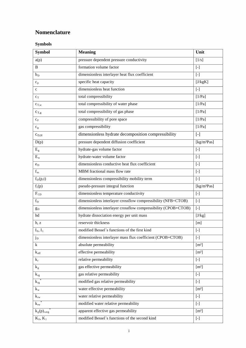
Nomenclature
Symbols
Symbol Meaning Unit
a(p) pressure dependent pressure conductivity [1/s] B formation volume factor [-] bD dimensionless interlayer heat flux coefficient [-] cp specific heat capacity [J/kgK] c dimensionless heat function [-] cT total compressibility [1/Pa] cT,w total compressibility of water phase [1/Pa]
cT,g total compressibility of gas phase [1/Pa]
cF compressibility of pore space [1/Pa] cg gas compressibility [1/Pa]
cD,H dimensionless hydrate decomposition compressibility [-]
D(p) pressure dependent diffusion coefficient [kg/m³Pas] Eg hydrate-gas volume factor [-]
Ew hydrate-water volume factor [-]
eD dimensionless conductive heat flux coefficient [-]
fm MBM fractional mass flow rate [-]
fD(p,t) dimensionless compressibility mobility term [-]
ft(p) pseudo-pressure integral function [kg/m³Pas]
FCD dimensionless temperature conductivity [-]
fD dimensionless interlayer crossflow compressibility (NFB+CTOB) [-]
gD dimensionless interlayer crossflow compressibility (CPOB+CTOB) [-]
hd hydrate dissociation energy per unit mass [J/kg]
h, z reservoir thickness [m]
I0, I1 modified Bessel´s functions of the first kind [-]
jD dimensionless interlayer mass flux coefficient (CPOB+CTOB) [-]
k absolute permeability [m²]
keff effective permeability [m²]
kr relative permeability [-]
kg gas effective permeability [m²]
krg gas relative permeability [-]
krg* modified gas relative permeability [-]
kw water effective permeability [m²]
krw water relative permeability [-]
krw* modified water relative permeability [-]
kg(p),avg* apparent effective gas permeability [m²]
K0, K1 modified Bessel´s functions of the second kind [-]
i

lD dimensionless distance to boundary [-]
ṁ mass flow rate [kg/s]
ṁtD dimensionless total mass flow rate [-]
nw water relative permeability exponent [-]
ng gas relative permeability exponent [-]
N hydrate permeability reduction exponent [-]
p reservoir pressure [Pa]
p Laplace complex variable [-]
Qst flow rate at standard conditions [m³/s]
R universal gas constant [J/molK]
rs(t), rs radius of dissociation [m]
rw wellbore radius [m]
rD dimensionless radius [-]
reD dimensionless drainage radius [-]
rsD dimensionless radius of dissociation [-]
S saturation [-]
S storativity [kg/m³Pa]
Sgirr connate gas saturation [-]
Swirr connate water saturation [-]
Sg,H gas saturation from hydrate dissociation [-]
Sw,H water saturation from hydrate dissociation [-]
SD modified dimensionless decomposition compressibility [-]
SDk modified dimensionless compressibility [-]
ss skin effect due to hydrate dissociation [-]
T temperature [°K]
t time [s]
tD dimensionless time [-]
tDw, tDwD dimensionless time with respect to wellbore [-]
tf* semi-log time for boundary dominated flow with single barrier [s]
ttf* derivative time for boundary dominated flow with single barrier [s]
w Darcy velocity [m/s]
V volume [m³]
dTeq/dp temperature gradient for hydrate dissociation [°C/Pa]
YD dimensionless interlayer mass flux coefficient (NFB+CTOB) [-]
zg gas compressibility factor [-]
ii
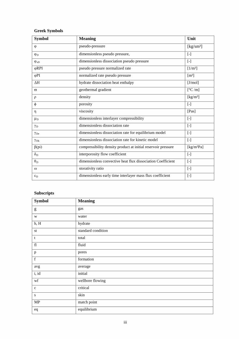
Greek Symbols
Symbol Meaning Unit φ pseudo-pressure [kg/sm³]
φD dimensionless pseudo pressure, [-] φsD dimensionless dissociation pseudo pressure [-] φRPI pseudo pressure normalized rate [1/m³] φPI normalized rate pseudo pressure [m³]
ΔH hydrate dissociation heat enthalpy [J/mol] ϖ geothermal gradient [°C /m] ρ density [kg/m³]
ϕ porosity [-]
η viscosity [Pas]
µD dimensionless interlayer compressibility [-]
γD dimensionless dissociation rate [-]
γDe dimensionless dissociation rate for equilibrium model [-]
γDk dimensionless dissociation rate for kinetic model [-]
β(pi) compressibility density product at initial reservoir pressure [kg/m³Pa]
δD interporosity flow coefficient [-]
θD dimensionless convective heat flux dissociation Coefficient [-]
ω storativity ratio [-]
εD dimensionless early time interlayer mass flux coefficient [-]
Subscripts
Symbol Meaning
g gas
w water h, H hydrate st standard condition t total
fl fluid
p pores
f formation
avg average
i, id initial
wf wellbore flowing
c critical
s skin
MP match point
eq equilibrium
iii
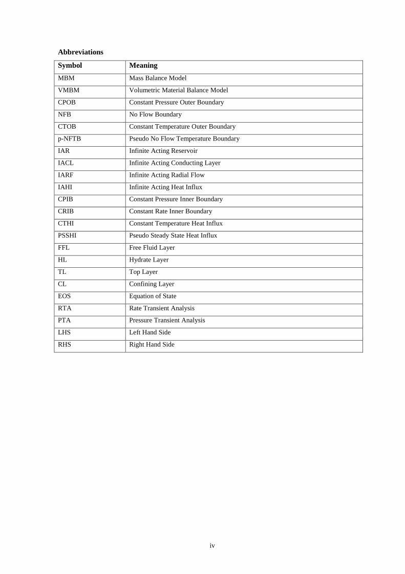
Abbreviations
Symbol Meaning MBM Mass Balance Model
VMBM Volumetric Material Balance Model CPOB Constant Pressure Outer Boundary
NFB No Flow Boundary
CTOB Constant Temperature Outer Boundary
p-NFTB Pseudo No Flow Temperature Boundary
IAR Infinite Acting Reservoir
IACL Infinite Acting Conducting Layer
IARF Infinite Acting Radial Flow
IAHI Infinite Acting Heat Influx
CPIB Constant Pressure Inner Boundary
CRIB Constant Rate Inner Boundary
CTHI Constant Temperature Heat Influx
PSSHI Pseudo Steady State Heat Influx
FFL Free Fluid Layer
HL Hydrate Layer
TL Top Layer
CL Confining Layer
EOS Equation of State
RTA Rate Transient Analysis
PTA Pressure Transient Analysis
LHS Left Hand Side
RHS Right Hand Side
iv
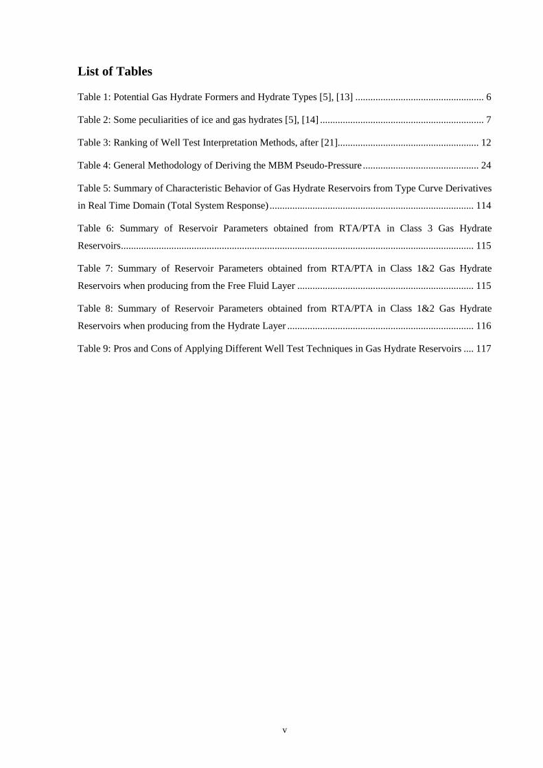
List of Tables
Table 1: Potential Gas Hydrate Formers and Hydrate Types [5], [13] ................................................... 6
Table 2: Some peculiarities of ice and gas hydrates [5], [14] ................................................................. 7
Table 3: Ranking of Well Test Interpretation Methods, after [21]........................................................ 12
Table 4: General Methodology of Deriving the MBM Pseudo-Pressure .............................................. 24
Table 5: Summary of Characteristic Behavior of Gas Hydrate Reservoirs from Type Curve Derivatives
in Real Time Domain (Total System Response) ................................................................................. 114
Table 6: Summary of Reservoir Parameters obtained from RTA/PTA in Class 3 Gas Hydrate
Reservoirs ............................................................................................................................................ 115
Table 7: Summary of Reservoir Parameters obtained from RTA/PTA in Class 1&2 Gas Hydrate
Reservoirs when producing from the Free Fluid Layer ...................................................................... 115
Table 8: Summary of Reservoir Parameters obtained from RTA/PTA in Class 1&2 Gas Hydrate
Reservoirs when producing from the Hydrate Layer .......................................................................... 116
Table 9: Pros and Cons of Applying Different Well Test Techniques in Gas Hydrate Reservoirs .... 117
v

List of Figures
Figure 1: Global Gas Hydrate Inventory [2] ........................................................................................... 1
Figure 2: Comparison of Gas Hydrate to other Fossil Resources (a, b) [after [4]] ................................. 2
Figure 3: Global map of recovered and inferred gas hydrates [7] ........................................................... 3
Figure 4: Microstructural Models for Hydrate Bearing Sediments [after [12]] ...................................... 4
Figure 5: Gas Hydrate Stability Zone in Permafrost Areas [modified after [3]] ..................................... 5
Figure 6: Gas Hydrate Stability Zone in Marine Areas [modified after [3]] ........................................... 5
Figure 7: Gas Hydrates; “Burning Ice Effect” [after Gary Klinkhammer [15]] ...................................... 6
Figure 8: Ideology of Gas Hydrate Production Techniques .................................................................... 8
Figure 9: Methodology of Reservoir Test Analysis [modified after [24]] ............................................ 10
Figure 10: I-S-O for Constant Terminal Rate ....................................................................................... 11
Figure 11: I-S-O for Constant Terminal Pressure ................................................................................. 11
Figure 12: Gas Hydrate Reservoir Classification [after [29]] ............................................................... 14
Figure 13: Crossflow Problems in Class 1 and 2 Gas Hydrates ............................................................ 14
Figure 14: Sensitivity of Equilibrium Pressure with Geothermal Gradient [30] ................................... 15
Figure 15: Workflow to Methodology of Applying the MMB Pseudo-pressure and the Energy Balance
(Equilibrium) Model ............................................................................................................................. 26
Figure 16: Comparison of the measured wellbore temperatures from the Mallik gas hydrate production
test of 2008 (Uddin, et al., 2012 [56]) with a Clausius Clapeyron type temperature depression model 27
Figure 17: Methodology of the Clausius Clapeyron Type Temperature Depression Model ................ 28
Figure 18: Methane Hydrate Equilibrium Curve and the Clausius Clapeyron Type Temperature
Depression Model ................................................................................................................................. 28
Figure 19: Methane Hydrate Equilibrium Curve and Methane Hydrate Heat of Dissociation ............. 29
Figure 20: Boundary Conditions for Heat Influx through Conduction (No Fluid Crossflow) .............. 29
Figure 21: Heat Influx Problems in Class 1 and 2 Gas Hydrate Reservoirs ......................................... 31
Figure 22: Material Balance Saturation and Relative Permeability with Pressure (Sgi =0.8, Swi=0.2,
ng=2, nw=4, Sgirr=0.02, Swirr=0.18) ....................................................................................................... 33
Figure 23: Material Balance Saturation and Relative Permeability with Pressure (Class 3 Hydrates,
neglecting heat conduction, Sgi =0.2, Swi=0.4, SHi=0.4, ng=2, nw=4, Sgirr=0.02, Swirr=0.18) ............... 33
Figure 24: Transient Rate Profile with Effects of Heat Energy Consumed in Hydrate Layer .............. 36
Figure 25: Derivative Plot for Rate Transient with Effects of Heat Energy Consumed in Hydrate Layer
............................................................................................................................................................... 37
Figure 26: Type-Curve Transient Rate Profile for Infinite Acting Reservoir-Constant Pressure at
Wellbore ................................................................................................................................................ 37
Figure 27: Dimensionless Pseudo-Profile for Infinite Acting Reservoir-Constant Pressure at Wellbore
............................................................................................................................................................... 38
vi
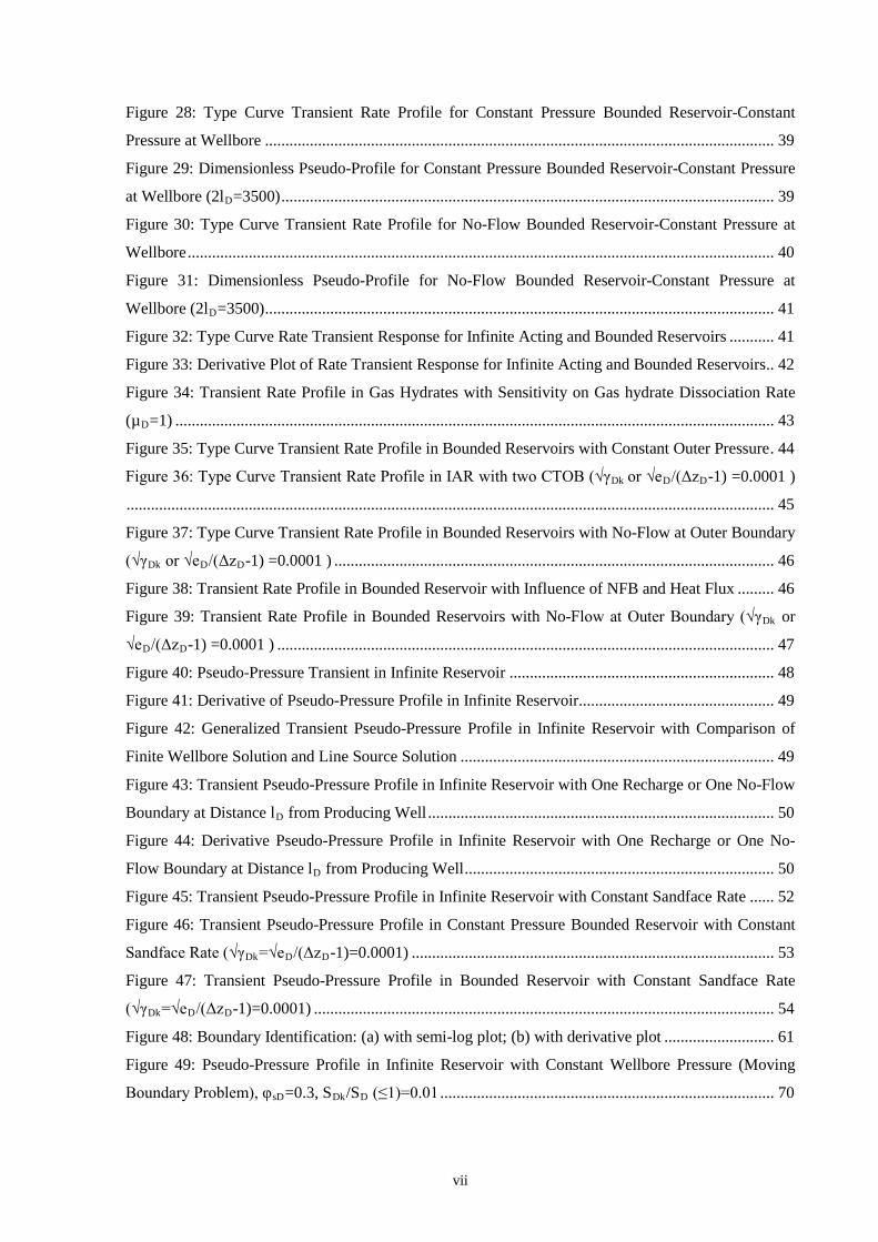
Figure 28: Type Curve Transient Rate Profile for Constant Pressure Bounded Reservoir-Constant
Pressure at Wellbore ............................................................................................................................. 39
Figure 29: Dimensionless Pseudo-Profile for Constant Pressure Bounded Reservoir-Constant Pressure
at Wellbore (2lD=3500) ......................................................................................................................... 39
Figure 30: Type Curve Transient Rate Profile for No-Flow Bounded Reservoir-Constant Pressure at
Wellbore ................................................................................................................................................ 40
Figure 31: Dimensionless Pseudo-Profile for No-Flow Bounded Reservoir-Constant Pressure at
Wellbore (2lD=3500) ............................................................................................................................. 41
Figure 32: Type Curve Rate Transient Response for Infinite Acting and Bounded Reservoirs ........... 41
Figure 33: Derivative Plot of Rate Transient Response for Infinite Acting and Bounded Reservoirs .. 42
Figure 34: Transient Rate Profile in Gas Hydrates with Sensitivity on Gas hydrate Dissociation Rate
(µD=1) ................................................................................................................................................... 43
Figure 35: Type Curve Transient Rate Profile in Bounded Reservoirs with Constant Outer Pressure . 44
Figure 36: Type Curve Transient Rate Profile in IAR with two CTOB (√γDk or √eD/(ΔzD-1) =0.0001 )
............................................................................................................................................................... 45
Figure 37: Type Curve Transient Rate Profile in Bounded Reservoirs with No-Flow at Outer Boundary
(√γDk or √eD/(ΔzD-1) =0.0001 ) ............................................................................................................ 46
Figure 38: Transient Rate Profile in Bounded Reservoir with Influence of NFB and Heat Flux ......... 46
Figure 39: Transient Rate Profile in Bounded Reservoirs with No-Flow at Outer Boundary (√γDk or
√eD/(ΔzD-1) =0.0001 ) .......................................................................................................................... 47
Figure 40: Pseudo-Pressure Transient in Infinite Reservoir ................................................................. 48
Figure 41: Derivative of Pseudo-Pressure Profile in Infinite Reservoir ................................................ 49
Figure 42: Generalized Transient Pseudo-Pressure Profile in Infinite Reservoir with Comparison of
Finite Wellbore Solution and Line Source Solution ............................................................................. 49
Figure 43: Transient Pseudo-Pressure Profile in Infinite Reservoir with One Recharge or One No-Flow
Boundary at Distance lD from Producing Well ..................................................................................... 50
Figure 44: Derivative Pseudo-Pressure Profile in Infinite Reservoir with One Recharge or One No-
Flow Boundary at Distance lD from Producing Well ............................................................................ 50
Figure 45: Transient Pseudo-Pressure Profile in Infinite Reservoir with Constant Sandface Rate ...... 52
Figure 46: Transient Pseudo-Pressure Profile in Constant Pressure Bounded Reservoir with Constant
Sandface Rate (√γDk=√eD/(ΔzD-1)=0.0001) ......................................................................................... 53
Figure 47: Transient Pseudo-Pressure Profile in Bounded Reservoir with Constant Sandface Rate
(√γDk=√eD/(ΔzD-1)=0.0001) ................................................................................................................. 54
Figure 48: Boundary Identification: (a) with semi-log plot; (b) with derivative plot ........................... 61
Figure 49: Pseudo-Pressure Profile in Infinite Reservoir with Constant Wellbore Pressure (Moving
Boundary Problem), φsD=0.3, SDk/SD (≤1)=0.01 .................................................................................. 70
vii
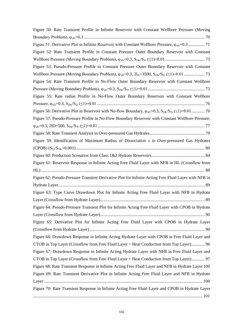
Figure 50: Rate Transient Profile in Infinite Reservoir with Constant Wellbore Pressure (Moving
Boundary Problem), φsD=0.3 ................................................................................................................ 70
Figure 51: Derivative Plot in Infinite Reservoir with Constant Wellbore Pressure, φsD=0.3 ............... 71
Figure 52: Rate Transient Profile in Constant Pressure Outer Boundary Reservoir with Constant
Wellbore Pressure (Moving Boundary Problem), φsD=0.3, SDk/SD (≤1)=0.01 ..................................... 73
Figure 53: Pseudo-Pressure Profile in Constant Pressure Outer Boundary Reservoir with Constant
Wellbore Pressure (Moving Boundary Problem), φsD=0.3, 2lD=3500, SDk/SD (≤1)=0.01 ................... 73
Figure 54: Rate Transient Profile in No-Flow Outer Boundary Reservoir with Constant Wellbore
Pressure (Moving Boundary Problem), φsD=0.3, SDk/SD (≤1)=0.01 ..................................................... 75
Figure 55: Rate radius Profile in No-Flow Outer Boundary Reservoir with Constant Wellbore
Pressure, φsD=0.3, SDk/SD (≤1)=0.01 .................................................................................................... 76
Figure 56: Derivative Plot in Reservoir with No-flow Boundary, φsD=0.3, SDk/SD (≤1)=0.01 ............ 76
Figure 57: Pseudo-Pressure Profile in No-Flow Boundary Reservoir with Constant Wellbore Pressure,
φsD=0.3, 2lD=500, SDk/SD (≤1)=0.01 ................................................................................................... 77
Figure 58: Rate Transient Analysis in Over-pressured Gas Hydrates ................................................... 79
Figure 59: Identification of Maximum Radius of Dissociation s in Over-pressured Gas Hydrates
(CPOB) (SD/SDk=0.001) ....................................................................................................................... 80
Figure 60: Production Scenarios from Class 1&2 Hydrate Reservoirs ................................................. 84
Figure 61: Reservoir Response in Infinite Acting Free Fluid Layer with NFB in HL (Crossflow from
HL) ........................................................................................................................................................ 88
Figure 62: Pseudo-Pressure Transient Derivative Plot for Infinite Acting Free Fluid Layer with NFB in
Hydrate Layer ........................................................................................................................................ 89
Figure 63: Type Curve Drawdown Plot for Infinite Acting Free Fluid Layer with NFB in Hydrate
Layer (Crossflow from Hydrate Layer)................................................................................................. 89
Figure 64: Pseudo-Pressure Transient Plot for Infinite Acting Free Fluid Layer with CPOB in Hydrate
Layer (Crossflow from Hydrate Layer)................................................................................................. 90
Figure 65: Derivative Plot for Infinite Acting Free Fluid Layer with CPOB in Hydrate Layer
(Crossflow from Hydrate Layer) ........................................................................................................... 90
Figure 66: Drawdown Response in Infinite Acting Hydrate Layer with CPOB in Free Fluid Layer and
CTOB in Top Layer (Crossflow from Free Fluid Layer + Heat Conduction from Top Layer) ............ 96
Figure 67: Drawdown Response in Infinite Acting Hydrate Layer with NFB in Free Fluid Layer and
CTOB in Top Layer (Crossflow from Free Fluid Layer + Heat Conduction from Top Layer) ............ 97
Figure 68: Rate Transient Response in Infinite Acting Free Fluid Layer and NFB in Hydrate Layer 100
Figure 69: Rate Transient Derivative Plot in Infinite Acting Free Fluid Layer and NFB in Hydrate
Layer ................................................................................................................................................... 100
Figure 70: Rate Transient Response in Infinite Acting Free Fluid Layer and CPOB in Hydrate Layer
............................................................................................................................................................. 101
viii
Figure 71: Rate Transient Response in Infinite Acting Hydrate Layer with NFB in Free Fluid Layer
and CTOB in Top Confining Layer .................................................................................................... 105
Figure 72: Rate Transient Response in Infinite Acting Hydrate Layer with CPOB in Free Fluid Layer
and CTOB in Top Confining Layer .................................................................................................... 106
ix
Chapter 1: Introduction
1 Introduction
In the last decade, a huge quest for unconventional reservoirs was perceived in the oil and gas
industry, which can be related to the unremittingly increasing energy demand coupled with the
depleting conventional reservoirs. As a result, unconventional reservoirs have become very attractive
in meeting up with this energy demand.
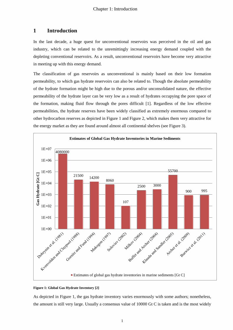
The classification of gas reservoirs as unconventional is mainly based on their low formation
permeability, to which gas hydrate reservoirs can also be related to. Though the absolute permeability
of the hydrate formation might be high due to the porous and/or unconsolidated nature, the effective
permeability of the hydrate layer can be very low as a result of hydrates occupying the pore space of
the formation, making fluid flow through the pores difficult [1]. Regardless of the low effective
permeabilities, the hydrate reserves have been widely classified as extremely enormous compared to
other hydrocarbon reserves as depicted in Figure 1 and Figure 2, which makes them very attractive for
the energy market as they are found around almost all continental shelves (see Figure 3).
Figure 1: Global Gas Hydrate Inventory [2]
As depicted in Figure 1, the gas hydrate inventory varies enormously with some authors; nonetheless,
the amount is still very large. Usually a consensus value of 10000 Gt C is taken and is the most widely
4080000
21500 14200 8060
107
2500 3000
55700
900 995
1E+00
1E+01
1E+02
1E+03
1E+04
1E+05
1E+06
1E+07
Gas
Hyd
rate
[Gt C
]
Estimates of Global Gas Hydrate Inventories in Marine Sediments
Estimates of global gas hydrate inventories in marine sediments [Gt C]
1
Chapter 1: Introduction
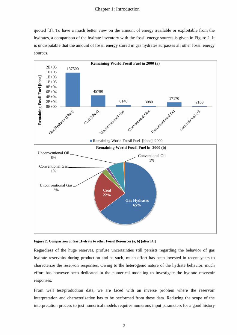
quoted [3]. To have a much better view on the amount of energy available or exploitable from the
hydrates, a comparison of the hydrate inventory with the fossil energy sources is given in Figure 2. It
is undisputable that the amount of fossil energy stored in gas hydrates surpasses all other fossil energy
sources.
Figure 2: Comparison of Gas Hydrate to other Fossil Resources (a, b) [after [4]]
Regardless of the huge reserves, profuse uncertainties still persists regarding the behavior of gas
hydrate reservoirs during production and as such, much effort has been invested in recent years to
characterize the reservoir responses. Owing to the heterogenic nature of the hydrate behavior, much
effort has however been dedicated in the numerical modeling to investigate the hydrate reservoir
responses.
From well test/production data, we are faced with an inverse problem where the reservoir
interpretation and characterization has to be performed from these data. Reducing the scope of the
interpretation process to just numerical models requires numerous input parameters for a good history
137500
45780
6140 3080 17170
2163 0E+002E+044E+046E+048E+041E+051E+051E+052E+05
Rem
aini
ng F
ossi
l Fue
l [bb
oe]
Remaining World Fossil Fuel in 2000 (a)
Remaining World Fossil Fuel [bboe], 2000
Gas Hydrates 65%
Coal 22%
Unconventional Gas 3%
Conventional Gas 1%
Unconventional Oil 8% Conventional Oil
1%
Remaining World Fossil Fuel in 2000 (b)
2
Chapter 1: Introduction
match. It should still be emphasized that inaccurate input parameters for any gas hydrate numerical
simulator can generate misleading predictions that would significantly affect further decisions in
relevant projects. The inaccuracy in input parameters associated with a numerical simulator can be
reduced with the use of reservoir testing characterization methods in conjunction with numerical
simulators for gas hydrates [1], which is as of now a field of great interest in the oil and gas industry.
However, for this process, a good understanding of the behavior of the hydrates and representative
conceptual models are required for the reservoir response. Next, we identify a few aspects regarding
gas hydrate and reservoir testing after which conceptual models will be developed to investigate the
responses expected from the hydrates during various production scenarios.
1.1 Gas Hydrates: Occurrence, Properties and Production
Gas hydrates are classified under the group of clathrates which is used to denote a molecule of a
substance enclosed in a structure built from molecules of other substances [5]. Hydrates in particular
are hence crystalline solid compounds with small molecules enclosed in water [5]. Since their
discovery in the early 19th century, gas hydrates only became of great interest in the oil and gas
industry with the inception of plugging of gas pipelines and other downstream equipment in the
1930´s. Gas hydrates were then a big foe for the upstream sector and measures were taken to mitigate
the occurrence of any hydrates.
1.1.1 Occurrence
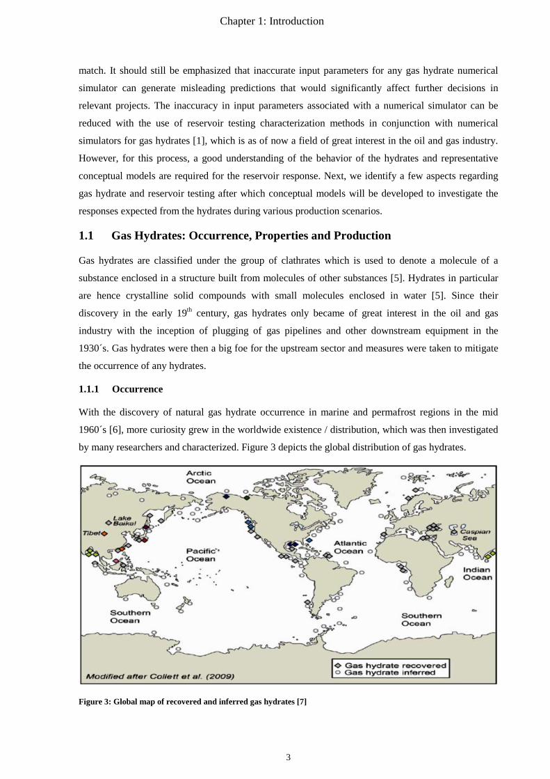
With the discovery of natural gas hydrate occurrence in marine and permafrost regions in the mid
1960´s [6], more curiosity grew in the worldwide existence / distribution, which was then investigated
by many researchers and characterized. Figure 3 depicts the global distribution of gas hydrates.
Figure 3: Global map of recovered and inferred gas hydrates [7]
3
Chapter 1: Introduction
From the global inventory, the next point of interest would be the amount of gas stored in the gas
hydrates which has been investigated and quantified by various authors [ [5], [8], [9], [10] ].
Nonetheless, for 1m³ methane hydrate we get approximately 164-180 Sm³ methane and about 0,8 Sm³
water [ [5], [10], [11] ]. The model required to estimate this conversion is developed using a mass
balance approach in Appendix 2.
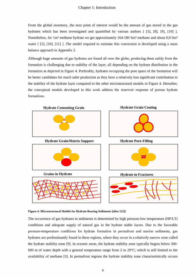
Although huge amounts of gas hydrates are found all over the globe, producing them safely from the
formation is challenging due to stability of the layer, all depending on the hydrate distribution in the
formation as depicted in Figure 4. Preferably, hydrates occupying the pore space of the formation will
be better candidates for much safer production as they have a relatively less significant contribution to
the stability of the hydrate layer compared to the other microstructural models in Figure 4. Hereafter,
the conceptual models developed in this work address the reservoir response of porous hydrate
formations.
Figure 4: Microstructural Models for Hydrate Bearing Sediments [after [12]]
The occurrence of gas hydrates in sediments is determined by high pressure-low temperature (HP/LT)
conditions and adequate supply of natural gas in the hydrate stable layers. Due to the favorable
pressure-temperature conditions for hydrate formation in permafrost and marine sediments, gas
hydrates are predominantly found in these regions, where they occur in a relatively narrow zone called
the hydrate stability zone [9]. In oceanic areas, the hydrate stability zone typically begins below 300-
600 m of water depth with a general temperature range from 2 to 20°C; which is still limited to the
availability of methane [3]. In permafrost regions the hydrate stability zone characteristically occurs
Hydrate Cementing Grain Hydrate Grain Coating
Hydrate Grain/Matrix Support Hydrate Pore-Filling
Grains in Hydrate Hydrate in Fractures
4
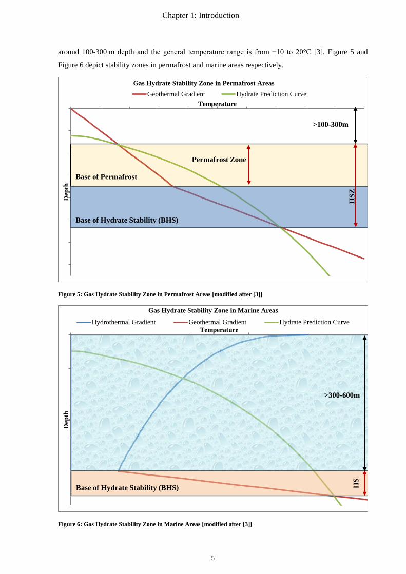
Chapter 1: Introduction
around 100-300 m depth and the general temperature range is from −10 to 20°C [3]. Figure 5 and
Figure 6 depict stability zones in permafrost and marine areas respectively.
Figure 5: Gas Hydrate Stability Zone in Permafrost Areas [modified after [3]]
Figure 6: Gas Hydrate Stability Zone in Marine Areas [modified after [3]]
Dep
th
Temperature
Gas Hydrate Stability Zone in Permafrost Areas Geothermal Gradient Hydrate Prediction Curve
Permafrost Zone
Base of Permafrost
Base of Hydrate Stability (BHS)
HSZ
>100-300m
Dep
th
Temperature
Gas Hydrate Stability Zone in Marine Areas
Hydrothermal Gradient Geothermal Gradient Hydrate Prediction Curve
Base of Hydrate Stability (BHS)
HS
>300-600m
5
Chapter 1: Introduction
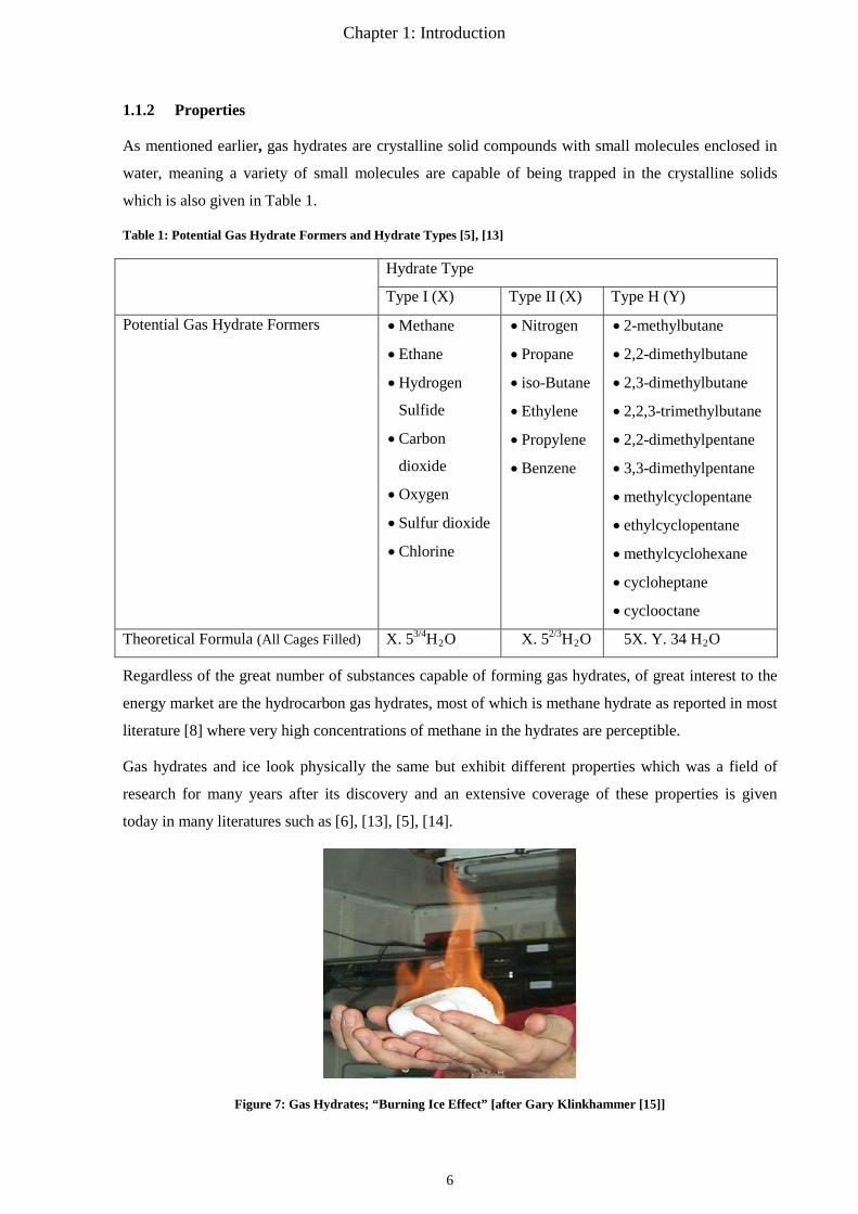
1.1.2 Properties
As mentioned earlier, gas hydrates are crystalline solid compounds with small molecules enclosed in
water, meaning a variety of small molecules are capable of being trapped in the crystalline solids
which is also given in Table 1.
Table 1: Potential Gas Hydrate Formers and Hydrate Types [5], [13]
Hydrate Type
Type I (X) Type II (X) Type H (Y)
Potential Gas Hydrate Formers • Methane
• Ethane
• Hydrogen
Sulfide
• Carbon
dioxide
• Oxygen
• Sulfur dioxide
• Chlorine
• Nitrogen
• Propane
• iso-Butane
• Ethylene
• Propylene
• Benzene
• 2-methylbutane
• 2,2-dimethylbutane
• 2,3-dimethylbutane
• 2,2,3-trimethylbutane
• 2,2-dimethylpentane
• 3,3-dimethylpentane
• methylcyclopentane
• ethylcyclopentane
• methylcyclohexane
• cycloheptane
• cyclooctane
Theoretical Formula (All Cages Filled) X. 53/4H2O X. 52/3H2O 5X. Y. 34 H2O
Regardless of the great number of substances capable of forming gas hydrates, of great interest to the
energy market are the hydrocarbon gas hydrates, most of which is methane hydrate as reported in most
literature [8] where very high concentrations of methane in the hydrates are perceptible.
Gas hydrates and ice look physically the same but exhibit different properties which was a field of
research for many years after its discovery and an extensive coverage of these properties is given
today in many literatures such as [6], [13], [5], [14].
Figure 7: Gas Hydrates; “Burning Ice Effect” [after Gary Klinkhammer [15]]
6
Chapter 1: Introduction
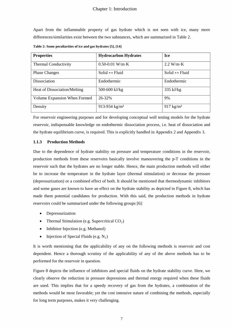
Apart from the inflammable property of gas hydrate which is not seen with ice, many more
differences/similarities exist between the two substances, which are summarized in Table 2.
Table 2: Some peculiarities of ice and gas hydrates [5], [14]
Properties Hydrocarbon Hydrates Ice
Thermal Conductivity 0.50-0.01 W/m·K 2.2 W/m·K
Phase Changes Solid ↔ Fluid Solid ↔ Fluid
Dissociation Endothermic Endothermic
Heat of Dissociation/Melting 500-600 kJ/kg 335 kJ/kg
Volume Expansion When Formed 26-32% 9%
Density 913-934 kg/m³ 917 kg/m³
For reservoir engineering purposes and for developing conceptual well testing models for the hydrate
reservoir, indispensable knowledge on endothermic dissociation process, i.e. heat of dissociation and
the hydrate equilibrium curve, is required. This is explicitly handled in Appendix 2 and Appendix 3.
1.1.3 Production Methods
Due to the dependence of hydrate stability on pressure and temperature conditions in the reservoir,
production methods from these reservoirs basically involve maneuvering the p-T conditions in the
reservoir such that the hydrates are no longer stable. Hence, the main production methods will either
be to increase the temperature in the hydrate layer (thermal stimulation) or decrease the pressure
(depressurization) or a combined effect of both. It should be mentioned that thermodynamic inhibitors
and some gases are known to have an effect on the hydrate stability as depicted in Figure 8, which has
made them potential candidates for production. With this said, the production methods in hydrate
reservoirs could be summarized under the following groups [6]:
• Depressurization
• Thermal Stimulation (e.g. Supercritical CO2)
• Inhibitor Injection (e.g. Methanol)
• Injection of Special Fluids (e.g. N2)
It is worth mentioning that the applicability of any on the following methods is reservoir and cost
dependent. Hence a thorough scrutiny of the applicability of any of the above methods has to be
performed for the reservoir in question.
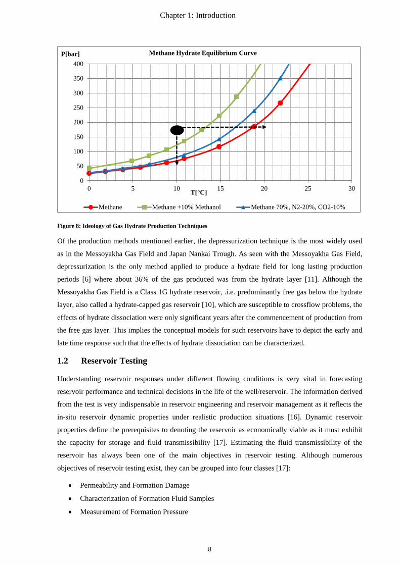
Figure 8 depicts the influence of inhibitors and special fluids on the hydrate stability curve. Here, we
clearly observe the reduction in pressure depressions and thermal energy required when these fluids
are used. This implies that for a speedy recovery of gas from the hydrates, a combination of the
methods would be most favorable; yet the cost intensive nature of combining the methods, especially
for long term purposes, makes it very challenging.
7
Chapter 1: Introduction
Figure 8: Ideology of Gas Hydrate Production Techniques
Of the production methods mentioned earlier, the depressurization technique is the most widely used
as in the Messoyakha Gas Field and Japan Nankai Trough. As seen with the Messoyakha Gas Field,
depressurization is the only method applied to produce a hydrate field for long lasting production
periods [6] where about 36% of the gas produced was from the hydrate layer [11]. Although the
Messoyakha Gas Field is a Class 1G hydrate reservoir, .i.e. predominantly free gas below the hydrate
layer, also called a hydrate-capped gas reservoir [10], which are susceptible to crossflow problems, the
effects of hydrate dissociation were only significant years after the commencement of production from
the free gas layer. This implies the conceptual models for such reservoirs have to depict the early and
late time response such that the effects of hydrate dissociation can be characterized.
1.2 Reservoir Testing
Understanding reservoir responses under different flowing conditions is very vital in forecasting
reservoir performance and technical decisions in the life of the well/reservoir. The information derived
from the test is very indispensable in reservoir engineering and reservoir management as it reflects the
in-situ reservoir dynamic properties under realistic production situations [16]. Dynamic reservoir
properties define the prerequisites to denoting the reservoir as economically viable as it must exhibit
the capacity for storage and fluid transmissibility [17]. Estimating the fluid transmissibility of the
reservoir has always been one of the main objectives in reservoir testing. Although numerous
objectives of reservoir testing exist, they can be grouped into four classes [17]:
• Permeability and Formation Damage
• Characterization of Formation Fluid Samples
• Measurement of Formation Pressure
0
50
100
150
200
250
300
350
400
0 5 10 15 20 25 30
P[bar]
T[°C]
Methane Hydrate Equilibrium Curve
Methane Methane +10% Methanol Methane 70%, N2-20%, CO2-10%
8
Chapter 1: Introduction
• Reservoir Characterization
The most common well testing methods include [17]:
• Open and cased hole wells with no completion string: DST
• Wireline Formation Testing: WFT
• Production /Injection Tests with Completion String
The deployment of any of the well test method is dependent on the objective of the well test and
highly determined by environment, safety, time and cost [18]. The volume of producible fluid from the
test method is very important as this defines the depth or radius of investigation of the reservoir. This
makes WFT restricted compared to DST and Production tests, as just the near wellbore vicinity can be
investigated with this method. A summary of DST and WFT types with pros and cons are
meticulously addressed in the literature [17], [19], [16], [18], [20].
1.2.1 Methodology of Reservoir Test Analysis
The methodology of reservoir test analysis is classified under two groups, all based on what
information is known about the reservoir. These include: the inverse and the direct problem.
Inverse (reverse) Problem
The inverse problem is characterized as the method of performing well test data analysis for reservoirs
with unknown behavior and has therefore a huge role in the characterization of the reservoir. Here, the
objective is to derive the interpretation model from the responses of the reservoir in question by
constantly verifying conceptual models which exhibit the same qualitative characteristics as the
system response [21]. Any false interpretation of the response at this stage will lead to wrong
forecasting and poor reservoir management. The more complex the reservoir, the more difficult it is to
identify the right model for the system, as ambiguity and non-uniqueness of the solution usually arises,
also intensified by the interpretation method implemented. However, conceptual models have to be
developed in order to properly identify the right reservoir model. Moreover, since diagnostic or
derivative plots [22] gained wide use in model identification, and more recently the application of
Deconvolution techniques [23], the identification process is becoming relatively less cumbersome.
Nonetheless, for this work, we will limit to simpler techniques as the complex reservoir behavior of
hydrates needs to be addressed first before more rigorous methods like the Convolution,
Deconvolution and Non-linear parameter estimation techniques [16] and their applicability are later
investigated.
SYTEM
(conceptual model)
SYSTEM
OUTPUT
INTEPRETATION AND RESERVOIR
CHARACTERIZATION
INPUT
9
Chapter 1: Introduction
Here the reservoir (system) characterization is derived from the measured reservoir response (output)
as a result of producing the well (input).
Direct (forward) Problem
In the direct problem, the reservoir model is known and hence analytical methods can be used to easily
solve the problem. Here, if any of the well test interpretation techniques are properly applied for the
known reservoir, the same results for the parameters will be achieved [21]. It should be noted that at
this level and due to the absence of field data in this work, just the direct problem can be addressed.
However, if the conceptual models are properly developed to represent the hydrate reservoir behavior,
well test analysis with the indirect method becomes easier.
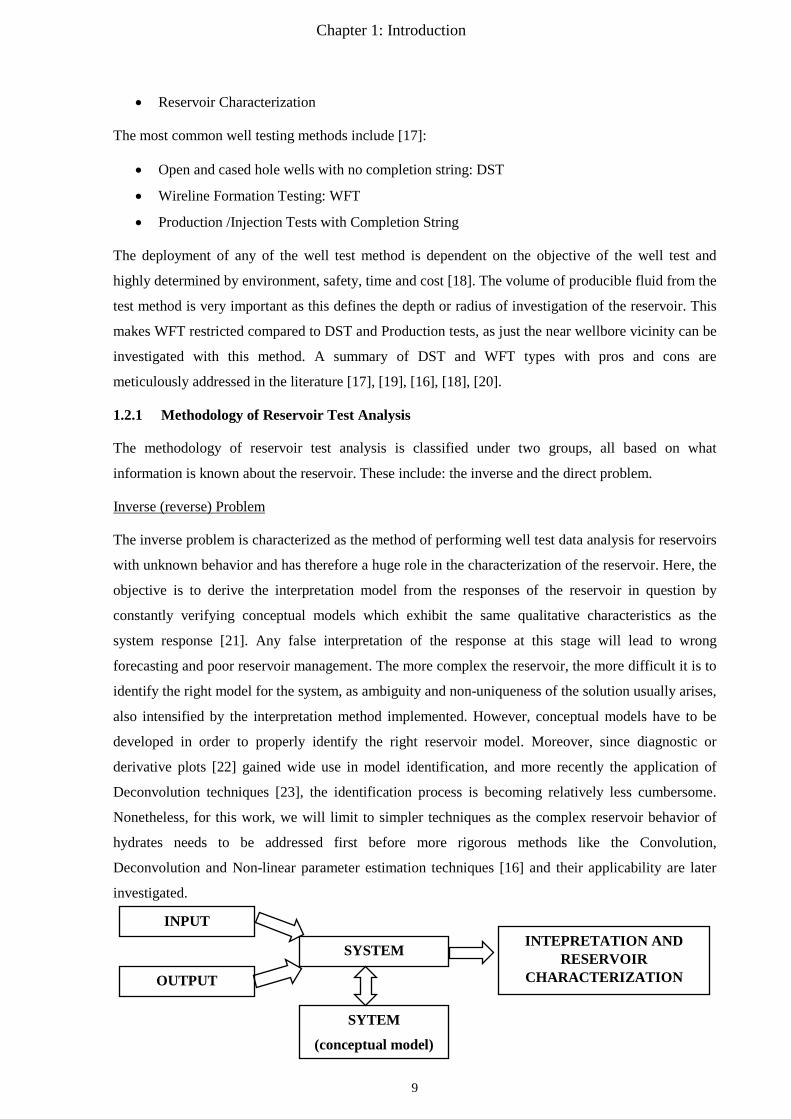
The workflow for the application of these methods is summarized once more below:
Figure 9: Methodology of Reservoir Test Analysis [modified after [24]]
INPUT
SYSTEM
OUTPUT INTEPRETATION AND RESERVOIR
CHARACTERIZATION
DIRECT PROBLEM INDIRECT PROBLEM
Formation and Geological Classification
Classify and Identify Flow Mechanism
Establish Well Test Model:
• Mathematical Model • Physical Model
Derive Solutions to Model:
• Analytical Solution • Numerical Solution
Derive Methods of Analysis
• Semi-log plots • Derivative Plots • Type Curves • Convolution/Deconvolution • Nonlinear Parameter Estimation • Cartesian Plots (Deliverability
Tests)
Repeat Interpretation
Result: Parameter Estimation
Identify Reservoir Model by Pressure/Rate Match
Well Test Interpretation
Model Analysis and Parameter Estimation
Identify Best Method of Analysis
• Semi-log plots • Derivative Plots • Type Curves • Convolution/Deconvolution • Nonlinear Parameter Estimation
Examine Test Data and Eliminate Anomaly Data
Acquire Pressure /Rate Data from Test
10
Chapter 1: Introduction
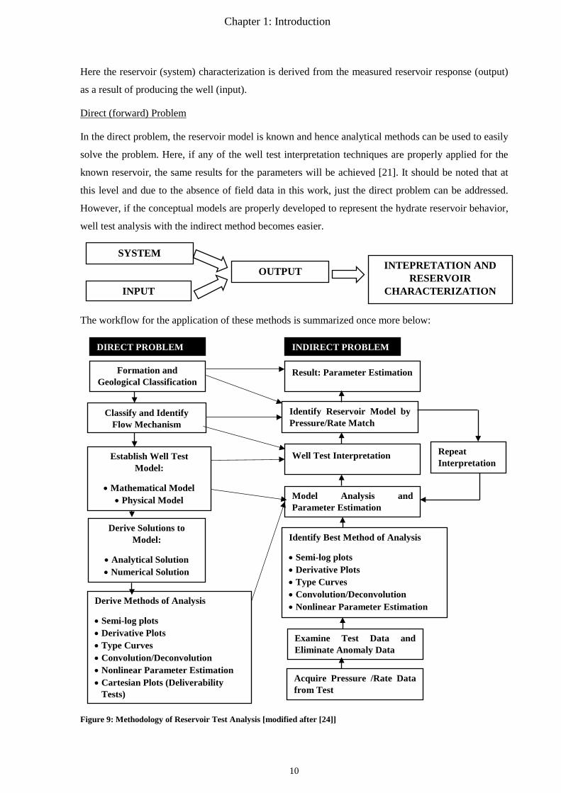
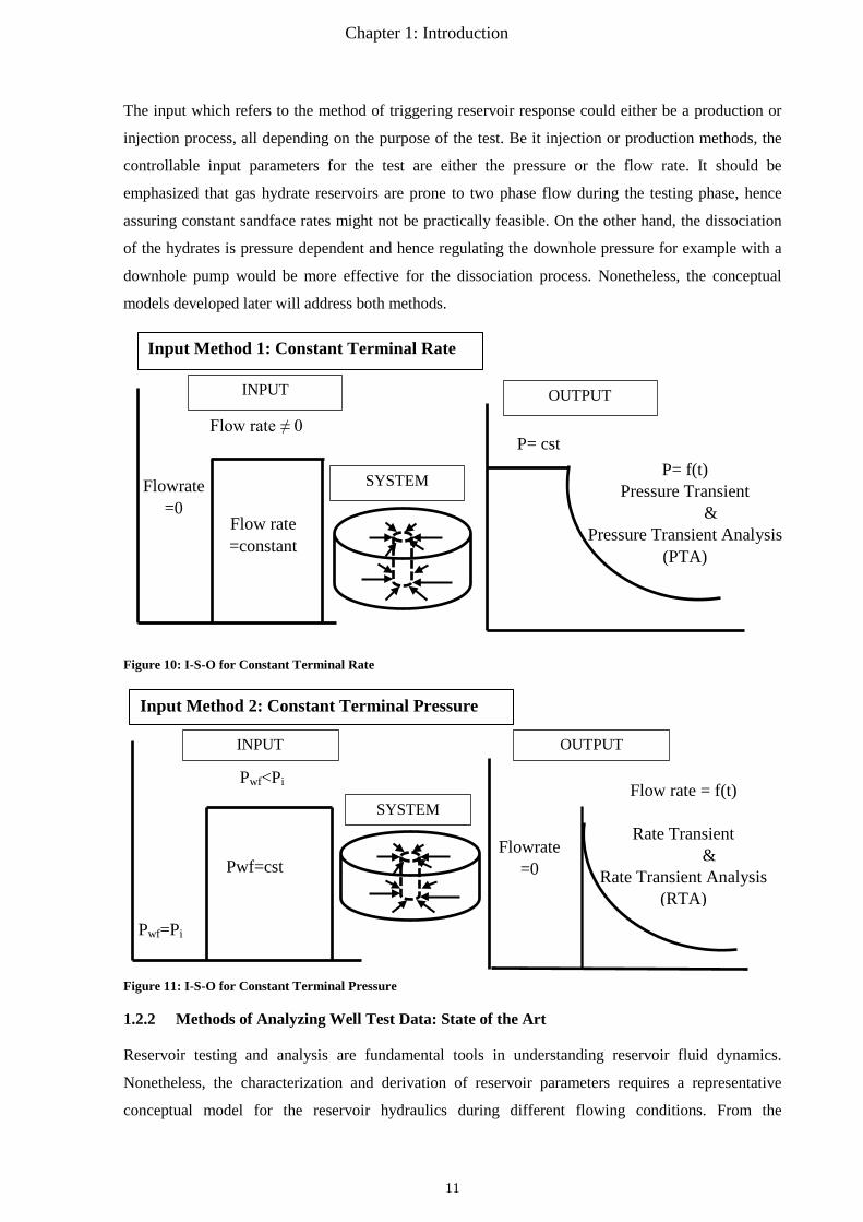
The input which refers to the method of triggering reservoir response could either be a production or
injection process, all depending on the purpose of the test. Be it injection or production methods, the
controllable input parameters for the test are either the pressure or the flow rate. It should be
emphasized that gas hydrate reservoirs are prone to two phase flow during the testing phase, hence
assuring constant sandface rates might not be practically feasible. On the other hand, the dissociation
of the hydrates is pressure dependent and hence regulating the downhole pressure for example with a
downhole pump would be more effective for the dissociation process. Nonetheless, the conceptual
models developed later will address both methods.
Figure 10: I-S-O for Constant Terminal Rate
Figure 11: I-S-O for Constant Terminal Pressure
1.2.2 Methods of Analyzing Well Test Data: State of the Art
Reservoir testing and analysis are fundamental tools in understanding reservoir fluid dynamics.
Nonetheless, the characterization and derivation of reservoir parameters requires a representative
conceptual model for the reservoir hydraulics during different flowing conditions. From the
P= cst P= f(t)
Pressure Transient &
Pressure Transient Analysis (PTA)
Input Method 1: Constant Terminal Rate
Flow rate ≠ 0
Flowrate =0
Flow rate =constant
INPUT OUTPUT
SYSTEM
Pwf=cst
Pwf<Pi
Pwf=Pi
Flowrate =0
Flow rate = f(t)
Rate Transient &
Rate Transient Analysis (RTA)
Input Method 2: Constant Terminal Pressure
INPUT OUTPUT
SYSTEM
11

Chapter 1: Introduction
conceptual models the choice of the method of analysis is built to qualitatively investigate the
behavior of the reservoir.
Methods of analysis can be classified under the following groups:
• Straight Lines or Semi-log Plots
• Type Curves
• Derivative Plots
• Deconvolution/Convolution
• Non-linear Parameter Estimation
Each of the above methods can be classified according to the accuracy of the analysis of well test data
and hence quality interpretation and characterization of the reservoir. Table 3 depicts the different
methods of analysis and strength in identifying reservoir parameters.
Table 3: Ranking of Well Test Interpretation Methods, after [21]
Date Analysis Method Identification
50s Straight lines Poor
70s Pressure Type Curves Fair
80s Pressure Derivative Very Good
Early 00s Deconvolution Much Better
Before the derivative or diagnostic plot became an indispensable and powerful tool in the analysis of
well test data, other methods of analysis such as semi-log straight line and type curves existed. The
evolution of new methods of analysis was backed by the growing complexity of the reservoir
responses, whereby straight line plots were difficult to obtain, heterogeneity and reservoir boundaries
were cumbersome to identify.
As will be shown later the following methods will be addressed for the characterization of gas hydrate
reservoirs:
• Solutions in Real Time Domain (Approximate Solutions to the Conceptual Models)
o semi-log
o type curves
o derivative
• Solutions in Laplace Domain (Exact Solutions to the Conceptual Models)
o Laplace Domain Well Test Model Recognition Type Curves
o Laplace Domain Well Test Model Recognition Derivatives
Although conventional methods such as the semi-log analysis and type curves in real time domain
have been addressed in this work, their limitations could be very significant due to the complex
12
Chapter 1: Introduction
behavior of the hydrate formations. However, the robust Laplace Domain Well Test Model
Recognition method proposed by [25] has proven to be a very effective tool in characterizing and
identifying different reservoir responses. Moreover, the application of derivatives in Laplace Domain
gives a much clearer representation of the different flow regimes during the hydrate dissociation
process.
The absence of field data makes the application of Deconvolution techniques or nonlinear parameter
estimation not practically feasible at this level. Although this method is becoming very useful and
robust in the interpretation process, it is still very rigorous at this level and also involves computer
aided analysis. Nevertheless, the methodology and development of algorithms are explicitly addressed
in several literatures including [23], [26], [27], [16], [28].
Note that the ranking in Table 3 is based on analysis of pressure transient data and shows that very
much has been done with regard to pressure transient analysis (PTA), which is not the case in rate
transient analysis (RTA), as PTA has been implemented over decades in the oil and gas industry while
RTA is still in its juvenile phase. Nonetheless, huge efforts are being made to qualitatively improve on
the methods of RTA, especially during infinite acting radial flow (IARF).
As will be shown later, rate transient models have been developed to investigate the response of the
hydrate reservoirs when subjected to constant wellbore pressure. This is very vital in gas hydrates as a
controllable dissociation of the hydrates is comparatively guaranteed using this method.
1.3 Reservoir Testing Challenges in Gas Hydrate Reservoirs
The complexity of reservoir response when producing from gas hydrate reservoirs is a known
phenomenon. This is reflected in the endothermic dissociation of the hydrates, gas and water
generation from the dissociation process and the two phase flow in the reservoirs. Moreover, the
hydrate layers are known to be unconsolidated which makes the choice of the wellbore flowing
pressure for dissociation very crucial to mitigate sand production. The choice and design of a well test
in such a reservoir should hence be carried out with great precaution.
Well test designs are carried out for each reservoir type in question, which means a characteristic
behavior of the reservoir needs to be known for a proper design process.
Though the dissociation of gas hydrates is conventionally handled similarly to the classical Stefan
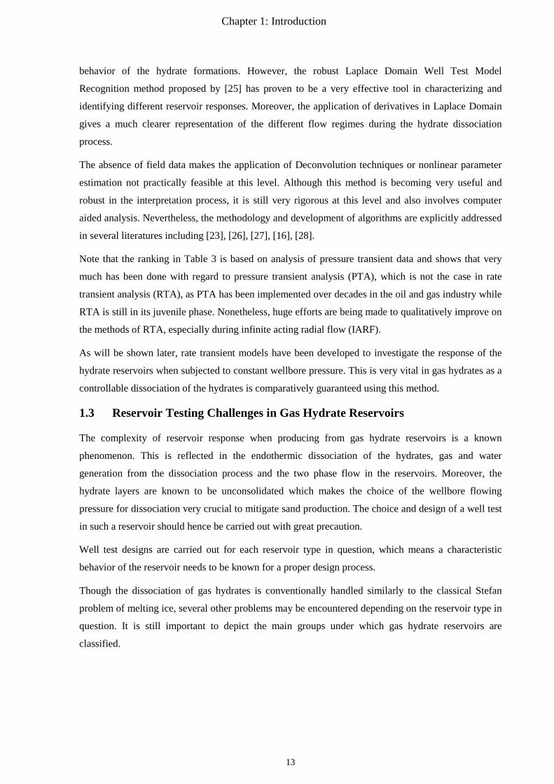
problem of melting ice, several other problems may be encountered depending on the reservoir type in
question. It is still important to depict the main groups under which gas hydrate reservoirs are
classified.
13
Chapter 1: Introduction
Figure 12: Gas Hydrate Reservoir Classification [after [29]]
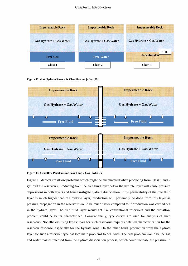
Figure 13: Crossflow Problems in Class 1 and 2 Gas Hydrates
Figure 13 depicts crossflow problems which might be encountered when producing from Class 1 and 2
gas hydrate reservoirs. Producing from the free fluid layer below the hydrate layer will cause pressure
depressions in both layers and hence instigate hydrate dissociation. If the permeability of the free fluid
layer is much higher than the hydrate layer, production will preferably be done from this layer as
pressure propagation in the reservoir would be much faster compared to if production was carried out
in the hydrate layer. The free fluid layer would act like conventional reservoirs and the crossflow
problem could be better characterized. Conventionally, type curves are used for analysis of such
reservoirs. Nonetheless using type curves for such reservoirs requires detailed characterization for the
reservoir response, especially for the hydrate zone. On the other hand, production from the hydrate
layer for such a reservoir type has two main problems to deal with. The first problem would be the gas
and water masses released from the hydrate dissociation process, which could increase the pressure in
Free Gas
Impermeable Rock
Gas Hydrate + Gas/Water
Class 1
Free Water
Impermeable Rock
Gas Hydrate + Gas/Water
Class 2
Impermeable Rock
Gas Hydrate + Gas/Water
Class 3
Underburden BHL
Free Fluid
Impermeable Rock
Gas Hydrate + Gas/Water
Free Fluid
Impermeable Rock
Gas Hydrate + Gas/Water
Free Fluid
Impermeable Rock
Gas Hydrate + Gas/Water
Free Fluid
Impermeable Rock
Gas Hydrate + Gas/Water
14
Chapter 1: Introduction
the reservoir as this would act like a source term in the hydrate layer, all depending on the hydrate
dissociation rate. Furthermore, if crossflow problems embark, further distortion of production data
could occur, where fluid influx is expected from the free fluid layer and increased hydrate dissociation
due to the warmer fluid from the free fluid layer. Though both hydrate dissociation and crossflow
problems could be quantified in a diffusivity problem and a well test model developed, the analysis of
such reservoir responses to get reservoir parameters is cumbersome as will be seen later.
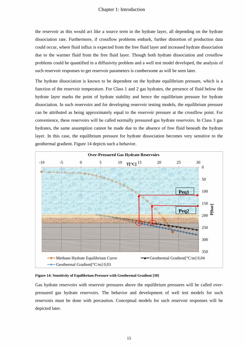
The hydrate dissociation is known to be dependent on the hydrate equilibrium pressure, which is a
function of the reservoir temperature. For Class 1 and 2 gas hydrates, the presence of fluid below the
hydrate layer marks the point of hydrate stability and hence the equilibrium pressure for hydrate
dissociation. In such reservoirs and for developing reservoir testing models, the equilibrium pressure
can be attributed as being approximately equal to the reservoir pressure at the crossflow point. For
convenience, these reservoirs will be called normally pressured gas hydrate reservoirs. In Class 3 gas
hydrates, the same assumption cannot be made due to the absence of free fluid beneath the hydrate
layer. In this case, the equilibrium pressure for hydrate dissociation becomes very sensitive to the
geothermal gradient. Figure 14 depicts such a behavior.
Figure 14: Sensitivity of Equilibrium Pressure with Geothermal Gradient [30]
Gas hydrate reservoirs with reservoir pressures above the equilibrium pressures will be called over-
pressured gas hydrate reservoirs. The behavior and development of well test models for such
reservoirs must be done with precaution. Conceptual models for such reservoir responses will be
depicted later.
0
50
100
150
200
250
300
350
-10 -5 0 5 10 15 20 25 30
P[ba
r]
T[°C]
Over-Pressured Gas Hydrate Reservoirs
Methane Hydrate Equilibrium Curve Geothermal Gradient[°C/m] 0,04Geothermal Gradient[°C/m] 0,03
Peq1
Peq2
15
Chapter 1: Introduction
To conclude, Class 1 and 2 gas hydrates could be further classified as normally pressured hydrate
reservoirs and crossflow is possible in these reservoirs. Class 3 gas hydrates could be normally
pressured or over-pressured, depending on the geothermal gradient. Crossflow problems here are
excluded. Due to the different responses expected from each reservoir type, well test design and
analysis have to be carried out depending on the reservoir type in question. The different well test
models for the different reservoir types will be handled in detail later.
1.3.1 Sand Production
Hydrate reservoirs are usually classified as unconsolidated formations, which means the formation
stability is low and the formation is prone to sand production if measures are not taken to mitigate this.
On the other hand, the dissociation of hydrates to produce gas and water is highly pressure and
temperature dependent. The higher the pressure depression, the more hydrates will dissociate to the
byproducts gas and water. Very high pressure depressions could be very detrimental in the stability of
the formation, which implies, sand production cases should be considered in the design process of the
well test.
1.3.2 Secondary Hydrate Formation in Tubing
High pressures and low temperatures in the tubing would provide favorable conditions for hydrates to
form during production of the two phase fluid system. Although depressurization at the sandface will
cause unfavorable conditions for hydrate formation, the decrease in temperature from the endothermic
dissociation could influence the formation of the hydrates. Moreover, if pumps are used for
depressurization and to lift the fluids to the surface, the increase in pressure at the pump outlet coupled
with the low temperature of the produced fluids (if the heat generated by the pump has little
significance) could highly influence the formation of secondary hydrates in the production string.
The formation of hydrates in the production string could highly affect the quality of the well test data
and furthermore, workover interventions might be needed to remove the hydrate plug in the
production string.
1.3.3 Hydrate Dissociation Model
Hydrates will dissociate to water and gas, meaning the hydrate dissociation process is basically a
source of water and gas in the porous medium. Describing the diffusivity equation therefore requires a
good description of the source term (hydrate dissociation); such that reservoir responses during
pressure depletion could be characterized and as such well test models derived for estimating reservoir
parameters. As of now, two main models exist in characterizing the hydrate dissociation rate.
Kinetic Model
The Kinetic Model for hydrate dissociation was developed by [31] based on laboratory experiments.
The model depicts the relationship between hydrate dissociation rates and pressure depressions. The
model proposed is given thus (see Appendix 1 for details):
16
Chapter 1: Introduction
dnhdt
= KdAH�peq − p� 1. 1
With: Kd [kmol/m²Pas], AH [m²], p [Pa], n [kmol]
The kinetic model is readily modified to:
dmHdt
= KdMHAH�peq − p� = Koe�−ERT�MHAH�peq − p� 1. 2
As also depicted in Appendix 4, the kinetic model reflects the dissociation of hydrates considering a
continuous constant source of heat energy, which limits the different sources of heat energy supplied
by the reservoir for hydrate dissociation as seen with the equilibrium model described in Appendix 1.
Hence the kinetic model encompasses all heat flux parameters and hence no further heat flux terms are
required when using the kinetic model. However, the wrong choice of the dissociation rate might
either overestimate or underestimate the rate of hydrate dissociation as defined by the equilibrium
model. Hence precaution should be taken when using the model in numerical simulators. For this
reason dimensionless parameters will be used to the conceptual models such that the reservoir
behavior under different dissociation conditions is characterized.
Equilibrium Model
The equilibrium model is an energy balance model which quantifies the heat energy available in the
reservoir and the quantity used up for every pressure depression. The model relates the dependence of
changes in reservoir heat energy with pressure and the energy required in dissociating the hydrates.
The application of the model at reservoir scale is much easier as the reservoir parameters can easily be
quantified; however, the reservoir testing model developed with the equilibrium model is more
complex as will be seen later. For numerical modeling purposes, where heat flux is better quantified,
the equilibrium model could be very useful as this better quantifies the heat energy in the reservoir and
the difficulty in quantifying the activation energy (E) and intrinsic rate constant (Ko) in the kinetic
model from laboratory scale to reservoir scale is avoided. Details on the equilibrium model are given
in Appendix 1-Appendix 4 for different production scenarios
1.4 Objectives and Structure of Thesis
Objectives of Thesis
From the various aspects and challenges addressed with regard to the hydrate behavior and problems
involving well testing in these reservoirs, the following are main objectives of this thesis:
• Develop conceptual models for gas hydrate reservoir testing which should aid in the
interpretation and characterization of gas hydrate reservoirs.
• Quantify different parameters which will affect the hydrate reservoir response during
production.
• Understand reservoir responses during production from different hydrate reservoir types.
17
Chapter 1: Introduction
• Investigate the behavior of the hydrate reservoirs with different productions scenarios based on
dimensionless parameters.
• Investigate the influential parameters during hydrate dissociation and identify the possible
influence on reservoir response.
• Identify non-linear reservoir parameters which might be very determining in applying future
more rigorous methods of analysis such as Deconvolution or nonlinear parameter estimation
methods.
• Assist numerical simulators in narrowing down uncertainties of reservoir parameters and
behavior from production data and hence reducing the non-uniqueness of the indirect reservoir
test analysis.
Structure of Thesis
Chapter 2 summaries the challenges and methodology involved in developing conceptual models in
these reservoir, which are also addressed in detail in the appendices.
Chapter 3 gives an overview of the approximate solutions to normally pressured class 3 gas hydrate
reservoirs with conventional methods of analysis applicable to specific reservoir responses.
Chapter 4 depicts the behavior over-pressured class 3 gas hydrate reservoir using similarity solutions
(approximate solutions).
Chapter 5 addresses crossflow problems in class 1 and 2 gas hydrate reservoirs considering the
possibility of producing from either the free fluid layer or the hydrate layer. Approximate solutions in
real time domain and conventional methods of analysis are addressed here.
Chapter 6 summarizes and concludes this thesis.
Appendices give a detailed derivation of the conceptual models for gas hydrate reservoirs. Bourgeois
and Horne Laplace domain well test model recognition method is addressed in detail for each reservoir
type, which gives a distinctive picture of the complexity of the reservoir behavior for each reservoir
type and a much better approach for reservoir characterization.
18
Chapter 2: Well Testing Models in Gas Hydrate Reservoirs: Challenges and Methodology
2 Well Testing Models in Gas Hydrate Reservoirs: Challenges and
Methodology
As described briefly in Chapter 1, production from hydrate reservoirs and the derivation of well test
models requires great precaution. The challenges faced with the derivation of conceptual models for
these reservoirs are summarized below:
• From the mass conservation principle used in deriving well test models, the hydrate
dissociation would be the source term in the diffusivity equation which is also endothermic.
Note that in conventional oil and gas reservoirs, source/sink terms are not commonly
addressed in reservoir testing models; moreover, the effect of endothermic process means the
temperature during depletion is not constant like in conventional reservoirs.
• Due to the hydrate dissociation byproducts, i.e. gas and water, we have two phase flow at
almost all times, provided the prevailing pressure is below the hydrate equilibrium pressure.
This implies multiphase flow has to be considered in all the models developed.
• The presence of gas in the system implies the consideration of the compressibility effects with
changes in pressure and temperature.
• The endothermic process during dissociation requires the consideration of heat flux in deriving
the well test model, which implies an energy balance approach to quantify the rate of heat
consumption for hydrate dissociation has to be applied. Note that isothermal conditions are
usually considered in conventional gas reservoirs, which cannot be applied here.
The dependence of most compressible and slightly compressible fluids with pressure in oil and gas
reservoirs triggers non-linear reservoir response, as pressure transient also affects reservoir fluid
properties. This problem was an issue of focus for many decades in the oil and gas industry till Al-
Hussainy [32] introduced the use of the Kirchhoff transformation in linearizing the diffusivity
equation in gas reservoirs. A further method of addressing the non-linearity of the diffusivity equation
with the Kirchhoff transformation was given by Agarwal [33] to address the problem of the changes in
the storativity term with time and pressure. In most of these methods, the permeability or effective
permeability of the fluids was considered constant and pressure independent. In recent years, with the
outburst of unconventional reservoirs or even conventional gas condensate reservoirs, the dependence
of the effective permeability of the phases became crucial and needed to be addressed. Multiphase
pseudo-pressures were then developed which addressed these effects (see Chapter 2.2 for details).
The problem of the dependence of the absolute permeability or effective permeability with pressure is
similar to concentration dependent diffusion coefficient problems addressed by many authors
including [34], [35], [36], [37], [38] . The authors proposed complex analytical solutions to the non-
linear diffusivity equation, most of which were solved by applying the Boltzmann transformation. It
should be emphasized that most of these mathematical methods considered single fluid phase
19

Chapter 2: Well Testing Models in Gas Hydrate Reservoirs: Challenges and Methodology
diffusivity problems which has however become obsolete in most diffusivity problems existing today,
whereby multiphase fluid flow has become a standard process.
In gas hydrate reservoirs, the problem of gas and water flow has to be addressed at almost all
production stages, as the hydrates will dissociate to gas and water; moreover, the hydrate layer could
be partly filled with water and gas. This gives the first source of the non-linear behavior. Secondly, the
endothermic dissociation of the hydrates causes temperature drop, increase in fluid saturation and
effective permeability. This implies, for a proper linearization of the diffusivity equation for gas
hydrate reservoirs, these processes need to be identified and quantified in the diffusivity equation.
Depending on the type of gas hydrate reservoir, different responses could be monitored during
production. In Class 1 and 2 gas hydrates, crossflow behavior is very possible and hence crossflow
problems would be addressed later. In Class 3 gas hydrate reservoirs, depending on the well test
method or the equilibrium pressure of the hydrate layer, different characteristic behaviors will be
observed such as the moving boundary problem which will be addressed in detail later.
Deriving the solution to non-linear diffusivity equations is gaining great interest in the oil and gas
industry due to the complex responses observed with unconventional oil and gas reservoirs.
For gas hydrate reservoirs, the following approaches will be made in deriving the solution to the
complex behavior:
Linearization
• Kirchhoff Transformation for the Multiphase Pseudo-pressure
The pressure dependent parameters in the diffusivity equation will be linearized using the Kirchhoff
transformation, analog [32] for gas pseudo-pressure and for two phase pseudo pressure in gas
condensate reservoirs [39], [40]. This is further addressed in Chapter 2.2. Note that although the
pressure dependent diffusion coefficient, reflected later in the mass balance model (MBM) or
volumetric material balance model (VMBM), is linearized using the Kirchhoff transformation, the
conceptual model for the gas hydrate has to address the changes in the multiphase pseudo-pressure as
a result of the dissociation effects as will be seen later.
Solutions
• Boltzmann Transformation (Similarity Solution)
• Laplace Transformations
The solutions for the diffusivity equation will be derived in dimensionless parameters using both the
Boltzmann Transformation and the Laplace Transformation for the following boundary conditions:
Inner Boundary Conditions
• Constant Rate Inner Boundary (CRIB) or Constant Terminal Rate (constant mass rate).
20
Chapter 2: Well Testing Models in Gas Hydrate Reservoirs: Challenges and Methodology
Unlike in conventional oil and gas well test models, the solutions presented here will be given
in pseudo-pressure and constant mass rate. The definition of the pseudo-pressure will be given
later.
• Constant Pressure Inner Boundary (CPIB) or Constant Terminal Pressure (constant multiphase
pseudo-pressure)
To develop the rate transient solutions using the CPIB, constant multiphase pseudo pressure conditions
are imposed on the wellbore, which is a preliminary to applying further well testing methods like
Deconvolution for changing inner boundary situations.
Outer Boundary Conditions
In deriving the solutions to the diffusivity equation, the following reservoir outer boundary
conditions are considered
• Infinite Acting Reservoir (IAR): r→∞; z→∞
• Constant Pressure Outer Boundary (CPOB): �dpdr�re
> 0; (dp)re = 0
• No-Flow Outer Boundary (NFB):�dpdr�re
= 0
• Constant Temperature Outer Boundary (CTOB): �dTdz�ze
> 0; (dT)ze = 0
• Pseudo No-Flow Temperature Boundary: �dTdz�ze
= 0
To investigate the effects of the reservoir boundaries on the wellbore response, the image well theory
is usually applied to the infinite acting solutions of the diffusivity problem. Note that the image well
theory proposed by [41] is one of the most widely used methods of investigating the wellbore response
of a reservoir with different kinds of boundaries as seen in the works of [41], [42], [43], [44]; however,
it is gradually being replaced by the use of Green´s functions. Although solutions for just single
boundaries are addressed in this work, it is important to develop a general solution for which the
image well theory could be investigated in future works. The image well theory is briefly discussed in
Appendix 8 for both similarity and Laplace domain solutions.
On the other hand, most of the solutions presented in this work for bounded reservoir using the
Bessel´s functions address reservoirs completely bounded by either a recharge or no-flow boundary
but not both, for which the well is located at the center. For this reason, the reservoir responses are
quite different from those derived with a single boundary using the image well theory.
2.1 Kirchhoff Transformation
In reservoir engineering, the Kirchhoff transformation is as of date, one of the most widely applied
methods of linearization of non-linear diffusivity equations. Its application is very much seen in
describing well test models in gas, gas condensate and Coalbed methane (CBM) reservoirs where the
21
Chapter 2: Well Testing Models in Gas Hydrate Reservoirs: Challenges and Methodology
fluid properties and flow are strongly pressure dependent. The diffusivity equation below depicts the
application of the transformation.
1r
∂�r∗D(p)∂p∂r�
∂r= S
𝑘𝑘∂p∂t
2. 1
From the above equation, the diffusion coefficient is pressure dependent. Instead of incorporating the
pressure dependent function of the diffusion coefficient, the Kirchhoff transformation is used.
Although the use of the Kirchhoff transformation is a well-established method of solving many
mathematical problems such as the pressure dependent diffusion coefficient problems [38], it only
gained huge significance through the works of [32] and [45]. Unlike other models such as the
solutions of [35] and [46] where the diffusion coefficient is assumed to behave in a particular manner
and the diffusivity equation solved, the Kirchhoff transformation offers the use of arbitrary functions
of the pressure dependent diffusion coefficient. The transformation is given below.
φ = ∫D(p)dp 2. 2
The Kirchhoff transformed diffusivity equation is hence:
1r
∂�r∂φ∂r�
∂r= S
kD(p)∂φ∂t
2. 3
1rD
∂�rD∂φ∂rD
�
∂rD= S
kD(p) rw2∂φ∂t
2. 4
1rD
∂�rD∂φ∂rD
�
∂rD= 1
a(p)∂φ∂t
2. 5
1rD
∂�rD∂φ∂rD
�
∂rD= 1
a(pi)a(pi)a(p)
∂φ∂t
2. 6
Although the pressure and the diffusion coefficients have been linearized, the diffusivity coefficient
can still be pressure dependent. Since the pressure in the reservoir is a function of time and radius, [33]
proposed the use of the pseudo-time integral by similarly applying the Kirchhoff transformation to the
time function. Nonetheless, the Agarwal pseudo-time considered just the dependence of the
Storativity, S; with pressure since gas reservoirs were considered. For incompressible fluids, the
storativity, S, is approximately constant or pressure independent, but this is not the case for
compressible fluids such as gas. For this reason, the pseudo-time is usually written thus:
ta = ∫ a(p)a�pi�
dt 2. 7
The precondition in applying these transformations is the functions in the integrals could be derived
for a given pressure. Recent innovations in the computation of pseudo-time for single phase gas
reservoirs are given in [47].
22
Chapter 2: Well Testing Models in Gas Hydrate Reservoirs: Challenges and Methodology
With the transformation of time and pressure using the Kirchhoff transformation, the equation is easily
simplified to the linearized form thus:
1rD
∂�rD∂φ∂rD
�
∂rD= 1
a(pi)∂φ∂ta
2. 8
∂2φ∂rD
2 + 1rD
∂φ ∂rD
= 1a(pi)
∂φ∂ta
2. 9
Linearization of the models is possible using the above methods of pseudo-pressure and pseudo-time,
however, analysis of real time and pressure data need a retransformation of the pseudo-parameters into
real time and pressure models such that reservoir parameters can be obtained.
Instead of using the Agarwal pseudo-time, other transformations can be made for the diffusivity
coefficient (with assumptions) such that the effects of hydrate dissociation on the reservoir response
can be investigated, especially when developing type curves. This will be shown in detail later.
2.2 Multiphase Diffusivity Equations for Well Testing
As mentioned earlier, dissociation of hydrates will result to gas and water production; hence,
multiphase flow is present in the reservoir at almost all times. For well test analysis, many multiphase
models have been developed with time; yet with limitations depending on the validity of mass
conservation which is a very useful principle used in many domains of fluid dynamics. The main
assumptions common in most multiphase well testing models used are negligible capillary pressure
and gravitation effects. With these assumptions, analytical models were proposed to describe
multiphase flow in reservoirs. It should be emphasized that existing models have considered several
other assumptions to simplify the diffusivity equation as much as possible which has also made their
applicability in some cases very limited. The three mainly used models for two-phase flow in the
reservoir are given below with validity of mass conservation [48].
2.2.1 Mass Balance Model (MBM)-State of the Art
The MBM, which can also be referred to as the composition model or EOS model type [49], is robust
and is derived directly from mass conservation principle and no major simplification of fluid
properties or further assumptions apart from the two stated above are made and is as of now the state
of the art in addressing multiphase flow in reservoirs. The mass balance model in radial coordinates is
given thus:
1r
∂(r∗�ρ1k1ɳ1+ρ2
k2ɳ2�∂p∂r)
∂r= ∅�ρ1cT,1 + ρ2cT,2�
∂p∂t
2. 10
The diffusivity equation above is developed from mass conservation principle and since no
simplification of the model has been done, mass conservation will always hold for the model.
Using the Kirchhoff transformation, pseudo-pressure models can be developed as also seen in CBM
and gas condensate reservoirs. The pseudo-pressure for this model is given thus:
23

Chapter 2: Well Testing Models in Gas Hydrate Reservoirs: Challenges and Methodology
φ = ∫ �ρ1k1ɳ1
+ ρ2k2ɳ2�dp 2. 11
The above model is a simplification of the reservoir integral as given by Jones and Raghavan [50] and
is the state of the art with regard to pseudo-pressure for multiphase systems also seen in other
literature such as [51], [52].
The general methodology of deriving the MBM pseudo-pressure is given in Table 4 for both rate
transient and pressure transient. Note that the pseudo-pressure is valid only if the parameters in the
pseudo-pressure integral are all pressure dependent.
Table 4: General Methodology of Deriving the MBM Pseudo-Pressure
RTA PTA
mt = mg + mw
↓
mt = 2πrhkρgkrg∗
ɳg∂p∂r
+ 2πrhkρwkrw∗
ɳwk∂p∂r
↓
mt(t)2πhk
∂rr
= �ρgkrg∗
ɳg+ ρw
krw∗
ɳw�∂p
↓
mt(t)2πhk(φi − φwf)
∂rr
=�ρg
krg∗ɳg
+ ρwkrw∗ɳw
� ∂p
(φi − φwf)
↓
mtD∂rDrD
=∂φ
(φi − φwf)
↓
�rD∂φD
∂rD�∂rDrD
=∂φ
(φi − φwf)
↓
φD =(φi − φ)
(φi − φwf)
mt = mg + mw
↓
mt = 2πrhkρgkrg∗
ɳg∂p∂r
+ 2πrhkρwkrw∗
ɳwk∂p∂r
↓
mt
2πhk∂rr
= �ρgkrg∗
ɳg+ ρw
krw∗
ɳw� ∂p
↓
∂rr
=2πhk
mt�ρg
krg∗
ɳg+ ρw
krw∗
ɳw� ∂p
↓
∂rr
=2πhk
mt∂φ
↓ ∂rDrD
=2πhk
mt∂φ = ∂φD
↓
lnrD =2πhk
mt(φi − φ) = φD
The workflow in Figure 15 depicts the methodology of applying the pseudo-pressure in combination
with the energy balance model derived in Appendix 1.
2.2.2 Volumetric Material Balance Model (VMBM)
The VMBM which can also be referred to as the black oil model type [ [49], [39]] can be considered
as a simplification of the MBM with the assumption the fluids have approximately equal densities at
standard or norm conditions and the model is given below:
1r
∂(r∗� k1B1ɳ1
+ k2B2ɳ2
�∂p∂r)
∂r= ∅�cT,1
B1+ cT,2
B2� ∂p∂t
2. 12
24
Chapter 2: Well Testing Models in Gas Hydrate Reservoirs: Challenges and Methodology
Since the densities of gas and water vary vastly from another at standard conditions, the model is not
appropriate for gas hydrate reservoirs. If undersaturated oil reservoirs are considered, with oil and
water flow, the errors however diminish [48]. The pseudo-pressure for this model is given thus:
φ = ∫ � k1B1ɳ1
+ k2B2ɳ2
�dp 2. 13
The above model is the obsolete version of the pseudo-pressure used previously to model gas
condensate and seen in several publications such as Boe [53].
2.2.3 Perrine Type VMBM
Another type of multiphase pseudo-pressure used for well testing is the Perrine Type VMBM, which is
an obsolete multiphase well testing model and a simplification of the MBM with the assumption that
the densities of the fluids are approximately equal and pressure independent.
Once more, the pressure of gas is pressure dependent and very different from that of water; this model
cannot be used for gas hydrate reservoirs. Nevertheless, with a look at undersaturated oil reservoirs
with basically oil and water as multiphase systems, the model can be applied to an extent. If the
Perrine [54] mobility is used, the pseudo-pressure for this model is given thus:
φ = ∫ �k1ɳ1 + k2ɳ2�dp 2. 14
The pseudo-pressure clearly indicates that the Perrine´s model is a modification of single phase flow
model [51] with the assumption of incompressible fluids.
All three models will yield the same results only for a single phase incompressible system. Note that
other rigorous multiphase diffusivity equations exist to address capillary pressure effects but still
difficult to implement for well test analysis purposes. A scrutiny of various multiphase diffusivity
equations is given in [55].
25
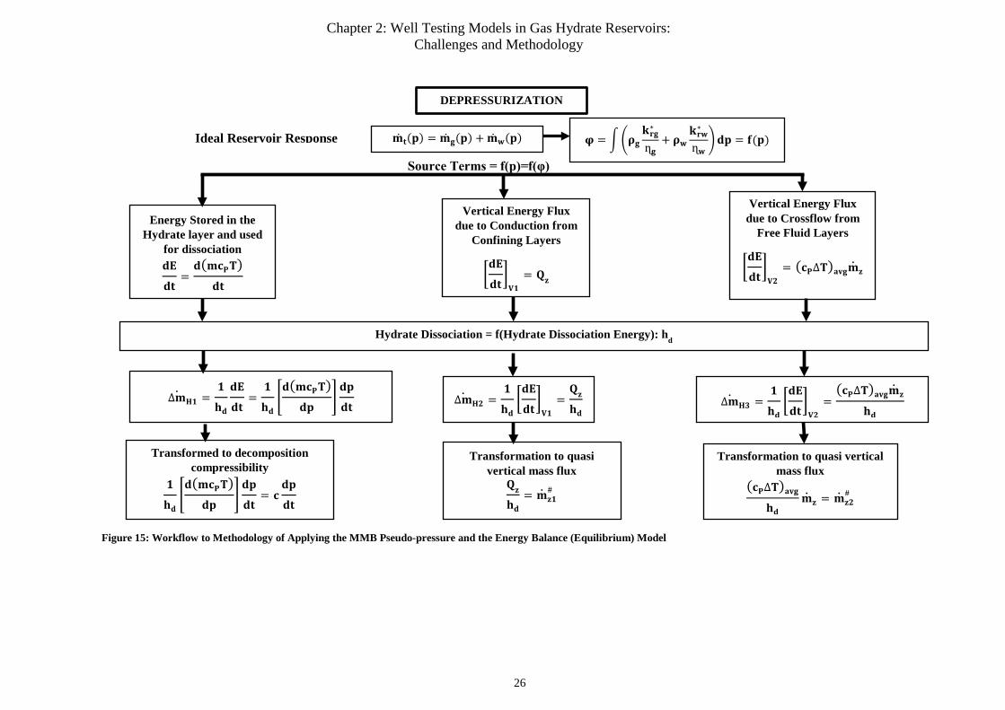
Chapter 2: Well Testing Models in Gas Hydrate Reservoirs: Challenges and Methodology
Figure 15: Workflow to Methodology of Applying the MMB Pseudo-pressure and the Energy Balance (Equilibrium) Model
DEPRESSURIZATION
𝐝𝐝𝐝𝐝
𝐝𝐝𝐝𝐝=𝐝𝐝(𝐦𝐦𝐦𝐦𝐏𝐏𝐓𝐓)
𝐝𝐝𝐝𝐝
Energy Stored in the Hydrate layer and used
for dissociation
∆��𝐦𝐇𝐇𝐇𝐇 =𝐇𝐇
𝐡𝐡𝐝𝐝
𝐝𝐝𝐝𝐝
𝐝𝐝𝐝𝐝=
𝐇𝐇
𝐡𝐡𝐝𝐝�𝐝𝐝(𝐦𝐦𝐦𝐦𝐏𝐏𝐓𝐓)
𝐝𝐝𝐝𝐝�𝐝𝐝𝐝𝐝
𝐝𝐝𝐝𝐝
𝐇𝐇
𝐡𝐡𝐝𝐝�𝐝𝐝(𝐦𝐦𝐦𝐦𝐏𝐏𝐓𝐓)
𝐝𝐝𝐝𝐝�𝐝𝐝𝐝𝐝
𝐝𝐝𝐝𝐝= 𝐦𝐦
𝐝𝐝𝐝𝐝
𝐝𝐝𝐝𝐝
Transformed to decomposition compressibility
�𝐝𝐝𝐝𝐝
𝐝𝐝𝐝𝐝�𝐕𝐕𝐇𝐇
= 𝐐𝐐𝐳𝐳
Vertical Energy Flux due to Conduction from
Confining Layers
�𝐝𝐝𝐝𝐝
𝐝𝐝𝐝𝐝�𝐕𝐕𝐕𝐕
= (𝐦𝐦𝐏𝐏∆𝐓𝐓)𝐚𝐚𝐚𝐚𝐚𝐚��𝐦𝐳𝐳
Vertical Energy Flux due to Crossflow from
Free Fluid Layers
∆��𝐦𝐇𝐇𝐕𝐕 =𝐇𝐇
𝐡𝐡𝐝𝐝�𝐝𝐝𝐝𝐝
𝐝𝐝𝐝𝐝�𝐕𝐕𝐇𝐇
=𝐐𝐐𝐳𝐳
𝐡𝐡𝐝𝐝 ∆��𝐦𝐇𝐇𝐇𝐇 =
𝐇𝐇
𝐡𝐡𝐝𝐝�𝐝𝐝𝐝𝐝
𝐝𝐝𝐝𝐝�𝐕𝐕𝐕𝐕
=(𝐦𝐦𝐏𝐏∆𝐓𝐓)𝐚𝐚𝐚𝐚𝐚𝐚��𝐦𝐳𝐳
𝐡𝐡𝐝𝐝
𝐐𝐐𝐳𝐳
𝐡𝐡𝐝𝐝= ��𝐦𝐳𝐳𝐇𝐇
#
Transformation to quasi vertical mass flux
(𝐦𝐦𝐏𝐏∆𝐓𝐓)𝐚𝐚𝐚𝐚𝐚𝐚𝐡𝐡𝐝𝐝
��𝐦𝐳𝐳 = ��𝐦𝐳𝐳𝐕𝐕#
Transformation to quasi vertical mass flux
Hydrate Dissociation = f(Hydrate Dissociation Energy): hd
��𝐦𝐝𝐝(𝐝𝐝) = ��𝐦𝐚𝐚(𝐝𝐝) + ��𝐦𝐰𝐰(𝐝𝐝) 𝛗𝛗 = ��𝛒𝛒𝐚𝐚𝐤𝐤𝐫𝐫𝐚𝐚∗
ɳ𝐚𝐚+ 𝛒𝛒𝐰𝐰
𝐤𝐤𝐫𝐫𝐰𝐰∗
ɳ𝐰𝐰�𝐝𝐝𝐝𝐝 = 𝐟𝐟(𝐝𝐝) Ideal Reservoir Response
Source Terms = f(p)=f(φ)
26

Chapter 2: Well Testing Models in Gas Hydrate Reservoirs: Challenges and Methodology
2.3 Heat Conduction and Hydrate Dissociation in Class 3 Hydrates
In Appendix 1, an energy balance model has been used to fully address the heat energy terms
responsible for hydrate dissociation. Note that the models are developed based on the assumption that
the inner boundary conditions for heat flux can be defined by a Clausius-Clapeyron Type Equilibrium
Model, which gives the dependence of pressure depressions to temperature depressions. This implies
the temperature profile in the hydrate layer is solely pressure dependent as long as hydrates are
present, as dissociation is endothermic and triggered by pressure depressions and also validates the use
of a pseudo-pressure model. Figure 16 also gives a comparison of the measured wellbore temperatures
from the Mallik gas hydrate production test of 2008 [56] with a Clausius Clapeyron type temperature
depression model and we notice a very small deviation between measured data and predicted data
(initial pressure of 110.05 bar and initial temperature 11.378°C; hence Peq and (dT/dp)eq can be
estimated according to Appendix 3). This further implies the model can be used as a relatively good
estimation without huge falsification of the prediction models.
Figure 16: Comparison of the measured wellbore temperatures from the Mallik gas hydrate production test of 2008
(Uddin, et al., 2012 [56]) with a Clausius Clapeyron type temperature depression model
The workflow below depicts the methodology of the application for the Clausius Clapeyron type
temperature depression model used in this work.
9,65 9,64 9,57 9,772 8,67 8,296
7,728
10,394 10,390 10,294 9,936
7,906 7,782 6,698
0
2
4
6
8
10
12
75,17882 75,14454 74,22926 70,84641 51,63496 50,46706 40,21442
Tw
f [°C
]
Pwf [bar]
Wellbore Flowing Temperature During Depressurization in Mallik 2L-38 Well vs Clausius Clapeyron Type Temperature Depression Model
(Production Test 2008)
Twf (measured) Twf (Clausius Clapeyron Type)
27
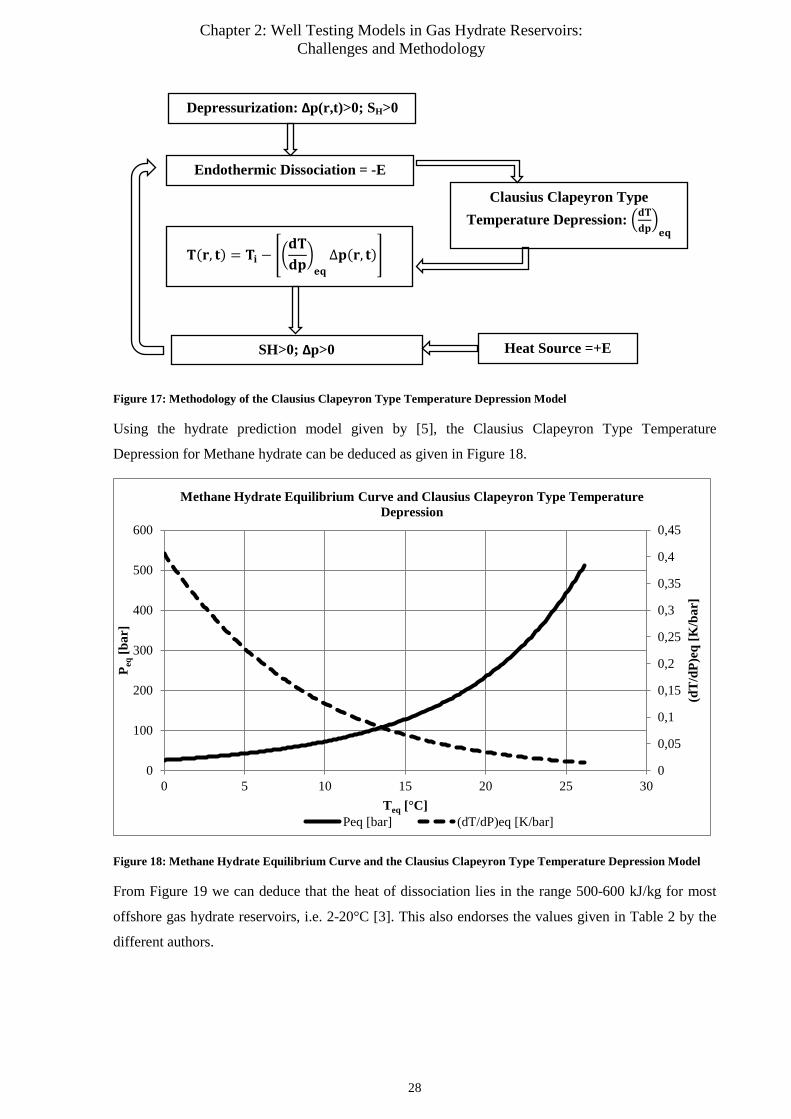
Chapter 2: Well Testing Models in Gas Hydrate Reservoirs: Challenges and Methodology
Figure 17: Methodology of the Clausius Clapeyron Type Temperature Depression Model
Using the hydrate prediction model given by [5], the Clausius Clapeyron Type Temperature
Depression for Methane hydrate can be deduced as given in Figure 18.
Figure 18: Methane Hydrate Equilibrium Curve and the Clausius Clapeyron Type Temperature Depression Model
From Figure 19 we can deduce that the heat of dissociation lies in the range 500-600 kJ/kg for most
offshore gas hydrate reservoirs, i.e. 2-20°C [3]. This also endorses the values given in Table 2 by the
different authors.
0
0,05
0,1
0,15
0,2
0,25
0,3
0,35
0,4
0,45
0
100
200
300
400
500
600
0 5 10 15 20 25 30
(dT
/dP)
eq [K
/bar
]
P eq [
bar]
Teq [°C]
Methane Hydrate Equilibrium Curve and Clausius Clapeyron Type Temperature Depression
Peq [bar] (dT/dP)eq [K/bar]
Endothermic Dissociation = -E
𝐓𝐓(𝐫𝐫, 𝐝𝐝) = 𝐓𝐓𝐢𝐢 − ��𝐝𝐝𝐓𝐓𝐝𝐝𝐝𝐝�𝐞𝐞𝐞𝐞∆𝐝𝐝(𝐫𝐫, 𝐝𝐝)�
SH>0; Δp>0 Heat Source =+E
Clausius Clapeyron Type Temperature Depression: �𝐝𝐝𝐓𝐓
𝐝𝐝𝐝𝐝�𝐞𝐞𝐞𝐞
Depressurization: Δp(r,t)>0; SH>0
28
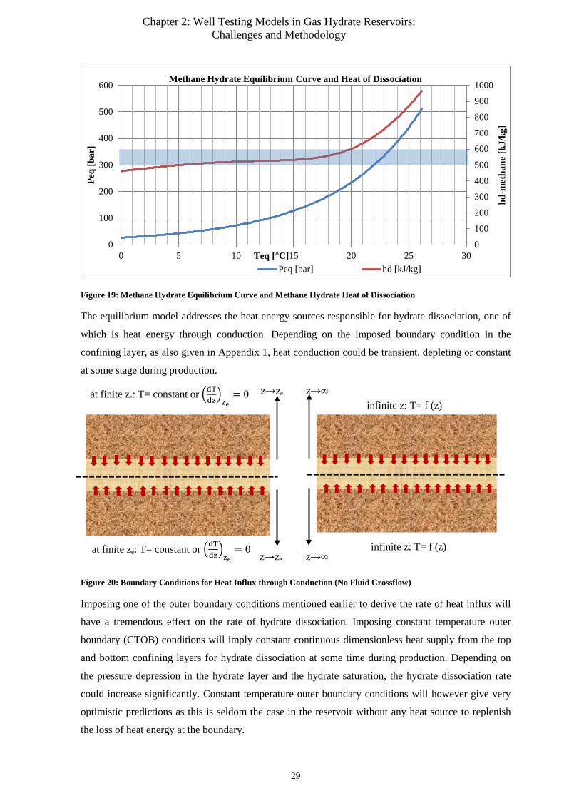
Chapter 2: Well Testing Models in Gas Hydrate Reservoirs: Challenges and Methodology
Figure 19: Methane Hydrate Equilibrium Curve and Methane Hydrate Heat of Dissociation
The equilibrium model addresses the heat energy sources responsible for hydrate dissociation, one of
which is heat energy through conduction. Depending on the imposed boundary condition in the
confining layer, as also given in Appendix 1, heat conduction could be transient, depleting or constant
at some stage during production.
Figure 20: Boundary Conditions for Heat Influx through Conduction (No Fluid Crossflow)
Imposing one of the outer boundary conditions mentioned earlier to derive the rate of heat influx will
have a tremendous effect on the rate of hydrate dissociation. Imposing constant temperature outer
boundary (CTOB) conditions will imply constant continuous dimensionless heat supply from the top
and bottom confining layers for hydrate dissociation at some time during production. Depending on
the pressure depression in the hydrate layer and the hydrate saturation, the hydrate dissociation rate
could increase significantly. Constant temperature outer boundary conditions will however give very
optimistic predictions as this is seldom the case in the reservoir without any heat source to replenish
the loss of heat energy at the boundary.
0
100
200
300
400
500
600
700
800
900
1000
0
100
200
300
400
500
600
0 5 10 15 20 25 30
hd-m
etha
ne [k
J/kg
]
Peq
[bar
]
Teq [°C]
Methane Hydrate Equilibrium Curve and Heat of Dissociation
Peq [bar] hd [kJ/kg]
at finite ze: T= constant or �dTdz�ze
= 0 z→ze
at finite ze: T= constant or �dTdz�ze
= 0 z→ze
infinite z: T= f (z)
infinite z: T= f (z) z→∞
z→∞
29
Chapter 2: Well Testing Models in Gas Hydrate Reservoirs: Challenges and Methodology
Due to the transient behavior of heat influx, the Laplace transformation would be a very useful tool in
developing the solutions to such a problem. It should be noted that the kinetic model assumes constant
heat source at all times during hydrate dissociation and is hence equivalent to the CTOB solution at
late production times. It is once more worth emphasizing that the heat flux in the infinite acting
vertical plane requires successive superposition of the solutions for each layer interval with a given
temperature as described by the geothermal gradient. The derivation of the solution to such a problem
could be very cumbersome, all depending on the thickness of the confining layer in question.
In general, at a given depth and production time, the temperature at the wellbore equals the
temperature of the infinite acting overburden as a result of the geothermal profile. The confining layer
then depicts a pseudo-NFB for heat influx although the system is infinite. This implies, in reality, the
heat support from the top layer would stop after a given production time and at a given depth as a
result of the decrease in the temperature of the reservoir with decreasing depth. For this reason, a
pseudo-NFTB model can be imposed on the reservoir response for the top layer. It is worth
mentioning that the pseudo-NFTB for heat influx is dependent on the degree of temperature
depression in the reservoir and the depth at which the reservoir temperature equals the temperature of
the confining layer. However, for the bottom layer, this would not be the case as temperature increases
with depth and hence heat influx from the bottom confining layer would be continuous and mask the
effect of the pseudo-NFB in the top confining layer.
To facilitate the computation of the heat influx and hence the hydrate dissociation rate, the temperature
in the confining layers will be assumed constant. As such, IAR, CTOB and p-NFTB conditions will be
imposed at the outer boundary to investigate the effects of heat influx on hydrate dissociation. This is
fully addressed in Appendix 12.
2.4 Heat Conduction, Convection and Hydrate Dissociation in Class 1 and 2
Hydrates
In Class 1 and 2 hydrates, the energy influx responsible for hydrate dissociation after pressure and
temperature drop in the hydrate layer is strongly dependent on the method of production. If the
reservoir is produced or tested from the free fluid layer, just heat conduction would be the additional
source of energy needed to be considered for hydrate dissociation as the cap rock above the hydrate
layer is considered impermeable. On the other hand, if the well is tested from the hydrate layer, heat
conduction from the top layer and convective heat transfer from the free fluid layer would have to be
considered as well.
30
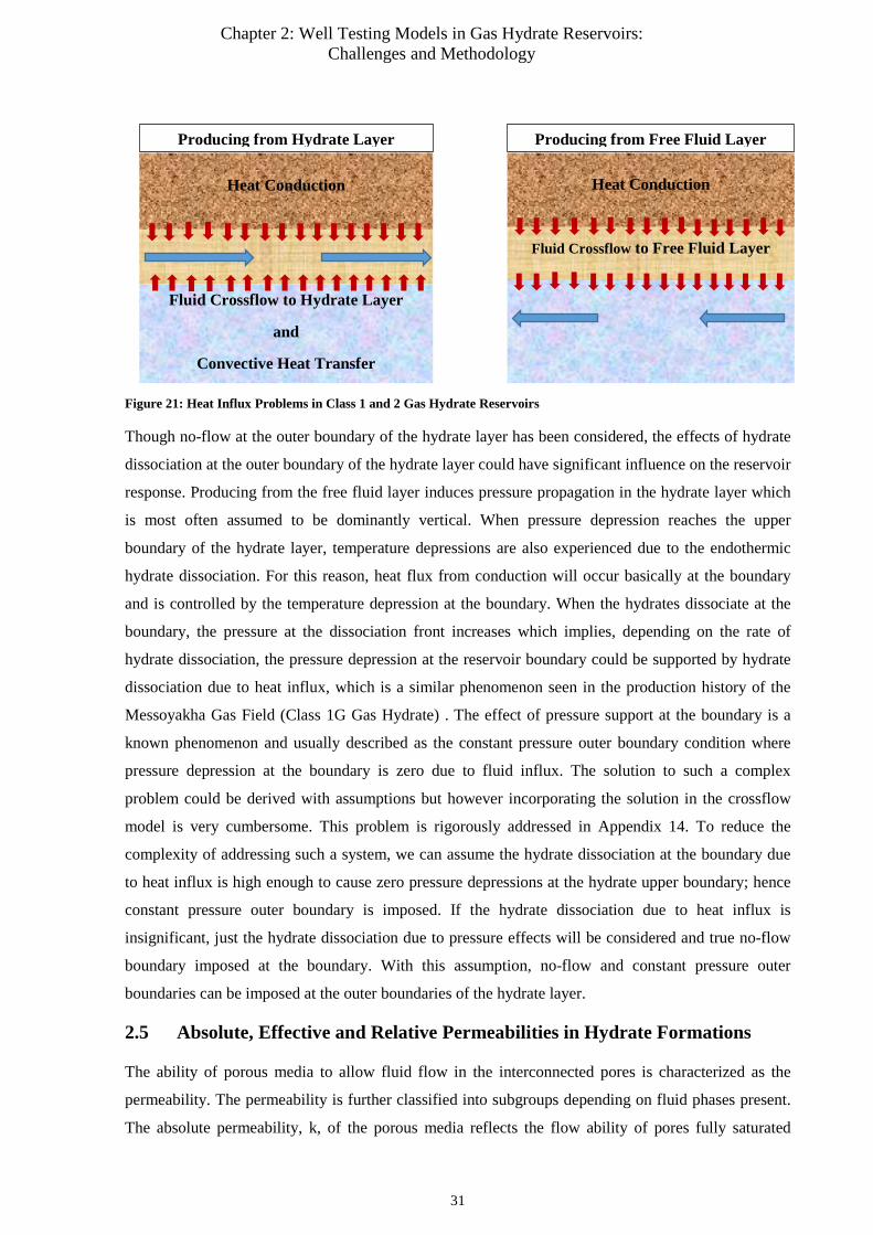
Chapter 2: Well Testing Models in Gas Hydrate Reservoirs: Challenges and Methodology
Figure 21: Heat Influx Problems in Class 1 and 2 Gas Hydrate Reservoirs
Though no-flow at the outer boundary of the hydrate layer has been considered, the effects of hydrate
dissociation at the outer boundary of the hydrate layer could have significant influence on the reservoir
response. Producing from the free fluid layer induces pressure propagation in the hydrate layer which
is most often assumed to be dominantly vertical. When pressure depression reaches the upper
boundary of the hydrate layer, temperature depressions are also experienced due to the endothermic
hydrate dissociation. For this reason, heat flux from conduction will occur basically at the boundary
and is controlled by the temperature depression at the boundary. When the hydrates dissociate at the
boundary, the pressure at the dissociation front increases which implies, depending on the rate of
hydrate dissociation, the pressure depression at the reservoir boundary could be supported by hydrate
dissociation due to heat influx, which is a similar phenomenon seen in the production history of the
Messoyakha Gas Field (Class 1G Gas Hydrate) . The effect of pressure support at the boundary is a
known phenomenon and usually described as the constant pressure outer boundary condition where
pressure depression at the boundary is zero due to fluid influx. The solution to such a complex
problem could be derived with assumptions but however incorporating the solution in the crossflow
model is very cumbersome. This problem is rigorously addressed in Appendix 14. To reduce the
complexity of addressing such a system, we can assume the hydrate dissociation at the boundary due
to heat influx is high enough to cause zero pressure depressions at the hydrate upper boundary; hence
constant pressure outer boundary is imposed. If the hydrate dissociation due to heat influx is
insignificant, just the hydrate dissociation due to pressure effects will be considered and true no-flow
boundary imposed at the boundary. With this assumption, no-flow and constant pressure outer
boundaries can be imposed at the outer boundaries of the hydrate layer.
2.5 Absolute, Effective and Relative Permeabilities in Hydrate Formations
The ability of porous media to allow fluid flow in the interconnected pores is characterized as the
permeability. The permeability is further classified into subgroups depending on fluid phases present.
The absolute permeability, k, of the porous media reflects the flow ability of pores fully saturated
Fluid Crossflow to Hydrate Layer
and
Convective Heat Transfer
Heat Conduction
Fluid Crossflow to Free Fluid Layer
Heat Conduction
Producing from Hydrate Layer Producing from Free Fluid Layer
31
Chapter 2: Well Testing Models in Gas Hydrate Reservoirs: Challenges and Methodology
(100%) with a single fluid phase [57]. In the presence of more than one phase in the pores, the term
effective permeability is introduced. The effective permeability and absolute permeability are related
by the following function:
keff = krk 2. 15
The term kr, denotes the relative permeability and it reflects the flow ability of a fluid relative to the
other fluid components present. Hence the effective permeability simply denotes the ability of the
porous media to allow flow of a given phase in the presence of another phase in the interconnected
pores.
In conventional gas reservoirs, two main fluid phases are common, which are gas and water. In
hydrate reservoirs, the presence of hydrates in the pores of the formation requires a further
classification of the permeability concepts. Masuda [58] carried out rigorous experimental studies on
hydrate dissociation and permeability changes and came up with the following correlation which is as
of now the most widely used in most numerical simulators:
kH = krHk = (1 − SH)Nk 2. 16
For convenience, the effective permeability of the gas and water phases will be represented thus:
kg = krgkH = �krg ∗ krH� ∗ k = krg∗ ∗ k 2. 17
kw = krwkH = (krw ∗ krH) ∗ k = krw∗ ∗ k 2. 18
Conventionally, fluid saturation, most especially gas, will decrease with pressure depletion. However;
in gas hydrates, this will not be the case as hydrates will dissociate to gas and water hence replenishing
the amount of gas withdrawn through production. The reservoir behavior in this case becomes a little
complex. The presence of gas, water and hydrate in the system and their changes with depletion
became an issue of concern as three phase relative permeability models had to be developed to address
such a response. As of now the most widely used three phase relative permeability model to address
hydrate behavior is the Stone [59] three phase model, modified by Aziz [55]. The effective and
relative permeabilities of the gas and water phases using this model are [10], [60]:
kg = krg∗ ∗ k = �Sg−Sgirr1−Sgirr
�ng
k 2. 19
kw = krw∗ ∗ k = �Sw−Swirr1−Swirr
�nw
k 2. 20
Note that the pseudo-pressures developed earlier relate the dependence of relative permeability with
pressure. To account for the changes in relative permeability with pressure the material balance
saturation models in Appendix 4 can be used.
32

Chapter 2: Well Testing Models in Gas Hydrate Reservoirs: Challenges and Methodology
Figure 22: Material Balance Saturation and Relative Permeability with Pressure (Sgi =0.8, Swi=0.2, ng=2, nw=4,
Sgirr=0.02, Swirr=0.18)
Figure 23: Material Balance Saturation and Relative Permeability with Pressure (Class 3 Hydrates, neglecting heat
conduction, Sgi =0.2, Swi=0.4, SHi=0.4, ng=2, nw=4, Sgirr=0.02, Swirr=0.18)
2.6 Boltzmann-Transformation (Similarity Variable Method)
The Boltzmann transformation is a very effective tool in transforming partial differential equations
into ordinary differential equations. The method simply involves the use a similarity variable, which is
a function of time and place, such that the derivatives of the variable can easily be incorporated into
the diffusivity equation, hence transforming it into an ordinary differential equation for which a
similarity solution can be obtained. In radial coordinates, the conventional Boltzmann similarity
variable with dimensionless time and radius is given thus:
vD2 = rD2
4tDw 2. 21
33
Chapter 2: Well Testing Models in Gas Hydrate Reservoirs: Challenges and Methodology
With the use of the above transformation complex methods of solving diffusivity equations could be
avoided. On the other hand, the transformation is not applicable in all radial flow problems for well
testing. The application of the Boltzmann transformation is given in Appendix 8.
The use of the Boltzmann transformation in solving the diffusivity equation analytically cannot be
used for all diffusivity problems, hence the use of more rigorous analytical methods such as Laplace
transforms are used. Nonetheless, most of the solutions of the diffusivity equations developed here
will be presented using both the Boltzmann and Laplace transforms.
2.7 Laplace-Transformation
The Laplace transformation is one of the most widely used methods of solving partial differential
equations in oil and gas reservoir engineering problems since its introduction by Van Everdingen and
Hurst [61]. It involves the transformation of the diffusivity equation in a Laplace domain form. The
Laplace transformation is given below:
L{f(t)} = ∫ e−pt∞0 f(t)dt = f(p) 2. 22
Applying the Laplace transform in the dimensionless diffusivity equation takes the form:
∂2𝐿𝐿(φ𝐷𝐷)∂rD
2 + 1rD
∂𝐿𝐿(φ𝐷𝐷) ∂rD
= ∫ e−ptDw∞0
∂φ𝐷𝐷∂tDw
dtDw 2. 23
∂2φ𝐷𝐷�∂rD
2 + 1rD
∂φ𝐷𝐷� ∂rD
= ∫ e−ptDw∞0 ∂φ𝐷𝐷 2. 24
∂2φ𝐷𝐷�∂rD
2 + 1rD
∂φ𝐷𝐷� ∂rD
= [−φ𝐷𝐷(𝑟𝑟𝐷𝐷, tDw = 0) + 𝑝𝑝φ𝐷𝐷� ] 2. 25
34
Chapter 3: Conceptual Models for Well Testing in Normally Pressured Class 3 Gas Hydrates
3 Conceptual Models for Well Testing in Normally Pressured Class 3
Gas Hydrates
The conceptual well testing models developed for the Class 3 gas hydrate reservoirs are developed based on the mass conservation principle as done in conventional oil and gas reservoirs, while considering the hydrate dissociation rate as the source term in the diffusivity equation.
As given in Appendix 5, the general mass conservation equation in radial coordinates is given thus:
2πh∆(r ∗ ρg ∗ wg) + 2πh∆(r ∗ ρw ∗ ww) = 2πrh∆r ∆�Sg∅ρg�∆t
+ 2πrh∆r ∆(Sw∅ρw)∆t
+ mH 3. 1
Based on the model used in addressing the hydrate dissociation rate, two different models can be generated for the response, namely:
Equilibrium Model
∂2φD∂rD2
+ 1rD
∂φD ∂rD
− �∂T𝑝𝑝𝐷𝐷∂z𝐷𝐷
�𝐶𝐶𝐶𝐶𝐶𝐶𝐶𝐶𝐶𝐶𝐶𝐶𝑘𝑘,𝑧𝑧𝐷𝐷=1
− �∂T𝑝𝑝𝐷𝐷∂z𝐷𝐷
�𝑈𝑈𝑈𝑈𝑈𝑈𝑈𝑈𝐶𝐶𝑈𝑈𝑈𝑈𝐶𝐶𝑈𝑈𝑈𝑈𝑈𝑈,𝑧𝑧𝐷𝐷=1
= SD∂φD∂tDw
3. 2
The above model takes the following form in Laplace domain by applying the temperature inner
boundary conditions addressed in Appendix 6:
∂2φ�D∂rD2
+ 1rD
∂φ�D ∂rD
− �SDp + �eDQpD� �
𝐶𝐶𝐶𝐶𝐶𝐶𝐶𝐶𝐶𝐶𝐶𝐶𝑘𝑘+ �eDQpD
� �𝑈𝑈𝑈𝑈𝑈𝑈𝑈𝑈𝐶𝐶𝑈𝑈𝑈𝑈𝐶𝐶𝑈𝑈𝑈𝑈𝑈𝑈
�φ�D = 0 3. 3
The above equation can simply be represented in the following form as also given in Appendix 7 and
Appendix 12:
∂2φ�D∂rD2
+ 1rD
∂φ�D ∂rD
− (SDp + γDe)φ�D = 0 3. 4
Kinetic Model
In the kinetic model, the hydrate dissociation rate is considered constant and hence the diffusivity
equation using this approach is written in time domain thus:
∂2φD∂rD2
+ 1rD
∂φD ∂rD
− γDkφD = SDk∂φD∂tDw
3. 5
The kinetic model in Laplace domain simply takes the form:
∂2φ�D∂rD2
+ 1rD
∂φ�D ∂rD
− (SDp + γDk)φ�D = 0 3. 6
The derivation of diffusivity equations of the normally pressured gas hydrate reservoir using the
kinetic and the equilibrium model are given in detail in Appendix 5.
The solutions to the above equation with constant pressure inner boundary (CPIB) and constant rate
inner boundary (CRIB) conditions using the Boltzmann and Laplace transforms are given in Appendix
12. The dimensionless pseudo-pressure and rate profiles are now depicted for the similarity solutions.
A meticulous overview of different and more complex reservoir responses are given in Appendix 12
with the Laplace domain well test model recognition method.
35
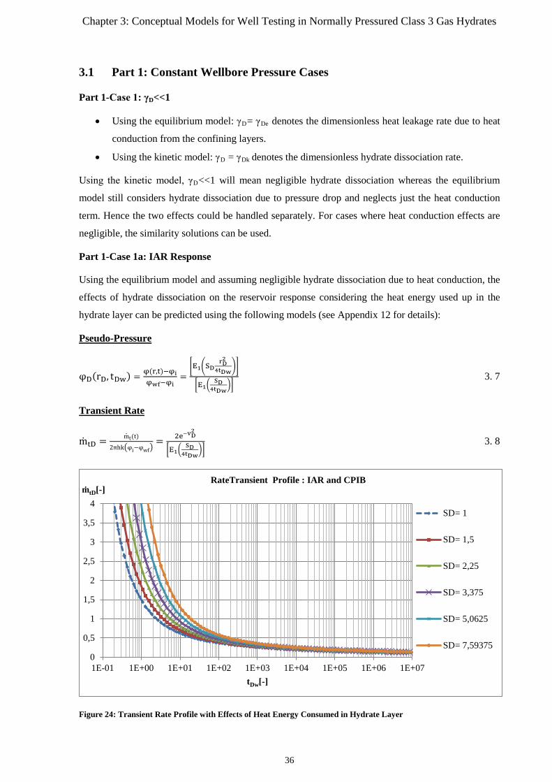
Chapter 3: Conceptual Models for Well Testing in Normally Pressured Class 3 Gas Hydrates
3.1 Part 1: Constant Wellbore Pressure Cases
Part 1-Case 1: γD<<1
• Using the equilibrium model: γD= γDe denotes the dimensionless heat leakage rate due to heat
conduction from the confining layers.
• Using the kinetic model: γD = γDk denotes the dimensionless hydrate dissociation rate.
Using the kinetic model, γD<<1 will mean negligible hydrate dissociation whereas the equilibrium
model still considers hydrate dissociation due to pressure drop and neglects just the heat conduction
term. Hence the two effects could be handled separately. For cases where heat conduction effects are
negligible, the similarity solutions can be used.
Part 1-Case 1a: IAR Response
Using the equilibrium model and assuming negligible hydrate dissociation due to heat conduction, the
effects of hydrate dissociation on the reservoir response considering the heat energy used up in the
hydrate layer can be predicted using the following models (see Appendix 12 for details):
Pseudo-Pressure
φD(rD, tDw) = φ(r,t)−φiφwf−φi
=�E1�SD
rD2
4tDw��
�E1�SD
4tDw��
3. 7
Transient Rate
mtD = mt(t)
2πhk�φi−φwf�= 2e−vD
2
�E1�SD
4tDw��
3. 8
Figure 24: Transient Rate Profile with Effects of Heat Energy Consumed in Hydrate Layer
0
0,5
1
1,5
2
2,5
3
3,5
4
1E-01 1E+00 1E+01 1E+02 1E+03 1E+04 1E+05 1E+06 1E+07
ṁtD[-]
tDw[-]
RateTransient Profile : IAR and CPIB
SD= 1
SD= 1,5
SD= 2,25
SD= 3,375
SD= 5,0625
SD= 7,59375
36
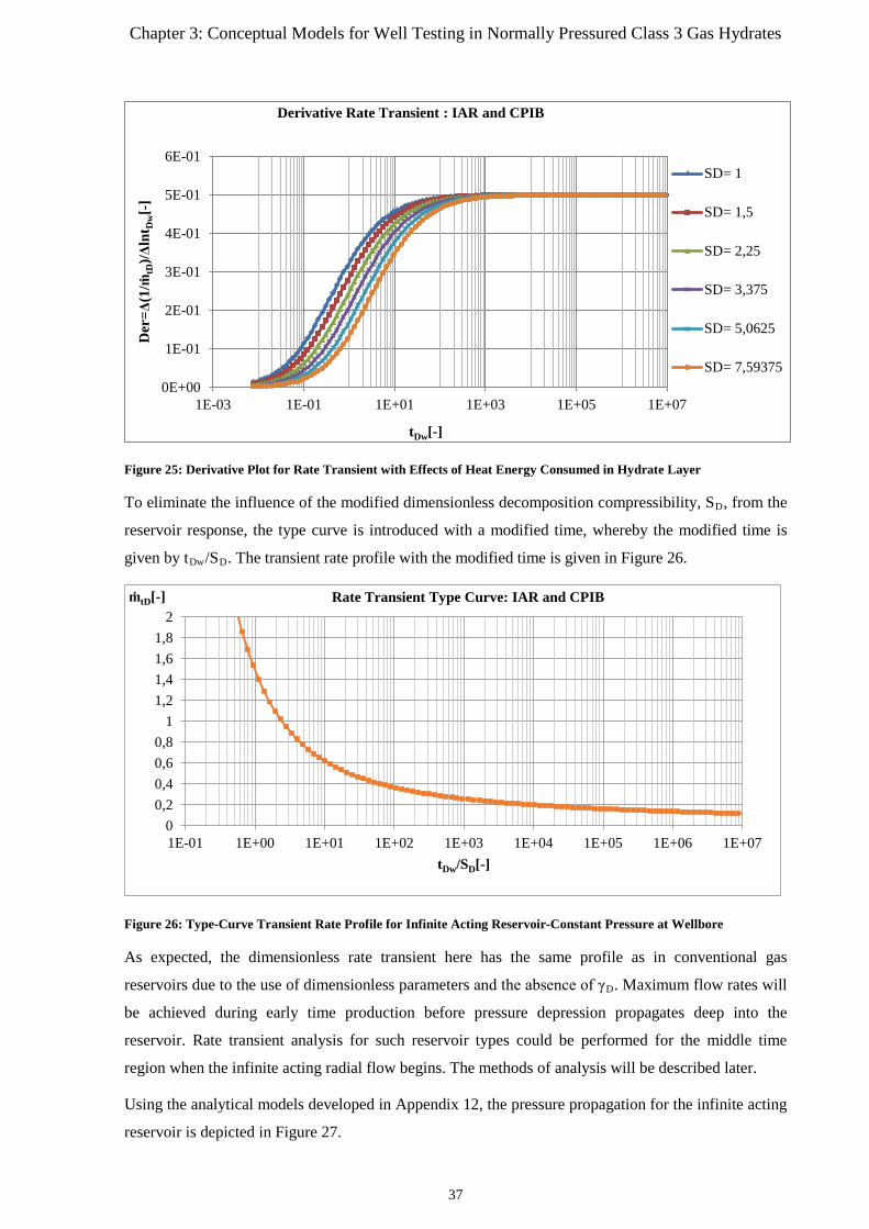
Chapter 3: Conceptual Models for Well Testing in Normally Pressured Class 3 Gas Hydrates
Figure 25: Derivative Plot for Rate Transient with Effects of Heat Energy Consumed in Hydrate Layer
To eliminate the influence of the modified dimensionless decomposition compressibility, SD, from the
reservoir response, the type curve is introduced with a modified time, whereby the modified time is
given by tDw/SD. The transient rate profile with the modified time is given in Figure 26.
Figure 26: Type-Curve Transient Rate Profile for Infinite Acting Reservoir-Constant Pressure at Wellbore
As expected, the dimensionless rate transient here has the same profile as in conventional gas
reservoirs due to the use of dimensionless parameters and the absence of γD. Maximum flow rates will
be achieved during early time production before pressure depression propagates deep into the
reservoir. Rate transient analysis for such reservoir types could be performed for the middle time
region when the infinite acting radial flow begins. The methods of analysis will be described later.
Using the analytical models developed in Appendix 12, the pressure propagation for the infinite acting
reservoir is depicted in Figure 27.
0E+00
1E-01
2E-01
3E-01
4E-01
5E-01
6E-01
1E-03 1E-01 1E+01 1E+03 1E+05 1E+07
Der
=Δ(1
/ṁtD
)/Δln
t Dw[-
]
tDw[-]
Derivative Rate Transient : IAR and CPIB
SD= 1
SD= 1,5
SD= 2,25
SD= 3,375
SD= 5,0625
SD= 7,59375
00,20,40,60,8
11,21,41,61,8
2
1E-01 1E+00 1E+01 1E+02 1E+03 1E+04 1E+05 1E+06 1E+07
ṁtD[-]
tDw/SD[-]
Rate Transient Type Curve: IAR and CPIB
37
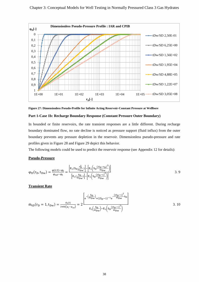
Chapter 3: Conceptual Models for Well Testing in Normally Pressured Class 3 Gas Hydrates
Figure 27: Dimensionless Pseudo-Profile for Infinite Acting Reservoir-Constant Pressure at Wellbore
Part 1-Case 1b: Recharge Boundary Response (Constant Pressure Outer Boundary)
In bounded or finite reservoirs, the rate transient responses are a little different. During recharge
boundary dominated flow, no rate decline is noticed as pressure support (fluid influx) from the outer
boundary prevents any pressure depletion in the reservoir. Dimensionless pseudo-pressure and rate
profiles given in Figure 28 and Figure 29 depict this behavior.
The following models could be used to predict the reservoir response (see Appendix 12 for details):
Pseudo-Pressure
φD(rD, tDw) = φ(r,t)−φiφwf−φi
=�E1(SD
rD2
4tDw)�−�E1�SD
�2lD−rD�2
4tDw��
�E1( SD4tDw
)�−�E1�SD�2lD−1�
2
4tDw��
3. 9
Transient Rate
mtD(rD = 1, tDw) = mt(t)
2πhk�φi−φwf�= 2
�e−�
SD4tDw
�+(2lD−1)−1e
−�2lD−1�
2
4tDwSD�
E1�SD
4tDw�−E1�SD
�2lD−1�2
4tDw�
3. 10
0
0,1
0,2
0,3
0,4
0,5
0,6
0,7
0,8
0,9
11E+00 1E+01 1E+02 1E+03 1E+04 1E+05
φD[-]
rD[-]
Dimensionless Pseudo-Pressure Profile : IAR and CPIB
tDw/SD 2,50E-01
tDw/SD 6,25E+00
tDw/SD 1,56E+02
tDw/SD 1,95E+04
tDw/SD 4,88E+05
tDw/SD 1,22E+07
tDw/SD 3,05E+08
38
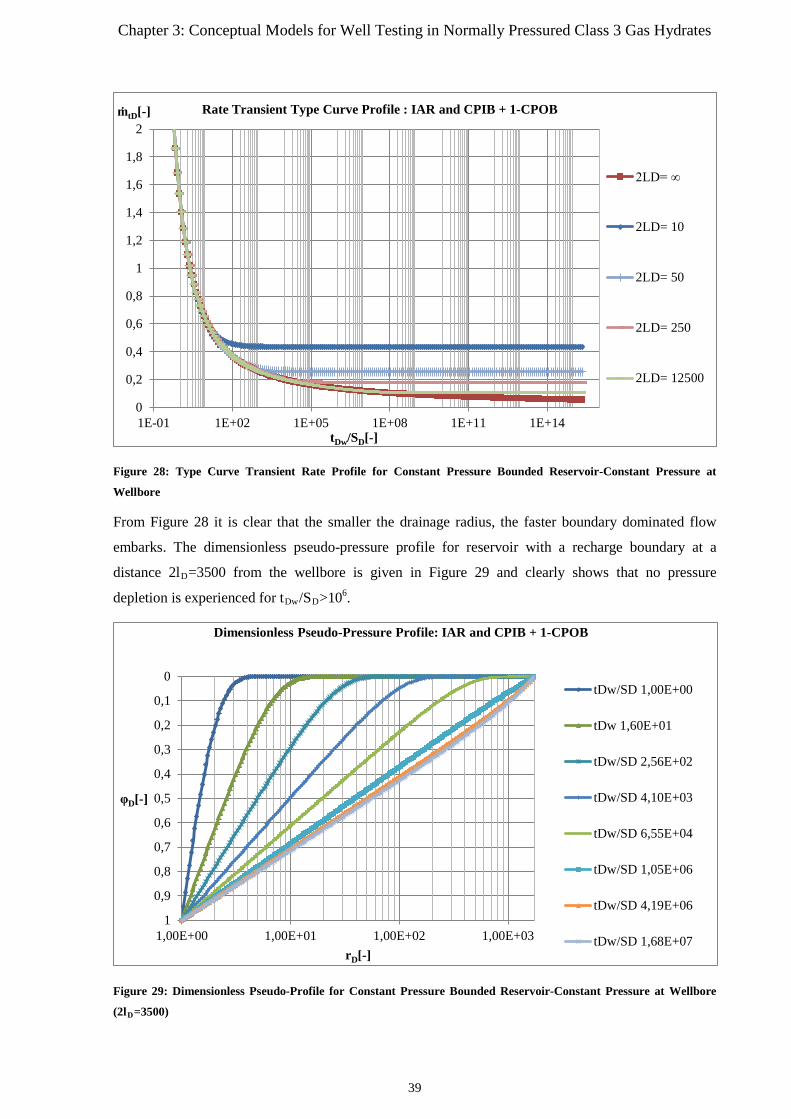
Chapter 3: Conceptual Models for Well Testing in Normally Pressured Class 3 Gas Hydrates
Figure 28: Type Curve Transient Rate Profile for Constant Pressure Bounded Reservoir-Constant Pressure at
Wellbore
From Figure 28 it is clear that the smaller the drainage radius, the faster boundary dominated flow
embarks. The dimensionless pseudo-pressure profile for reservoir with a recharge boundary at a
distance 2lD=3500 from the wellbore is given in Figure 29 and clearly shows that no pressure
depletion is experienced for tDw/SD>106.
Figure 29: Dimensionless Pseudo-Profile for Constant Pressure Bounded Reservoir-Constant Pressure at Wellbore
(2lD=3500)
0
0,2
0,4
0,6
0,8
1
1,2
1,4
1,6
1,8
2
1E-01 1E+02 1E+05 1E+08 1E+11 1E+14
ṁtD[-]
tDw/SD[-]
Rate Transient Type Curve Profile : IAR and CPIB + 1-CPOB
2LD= ∞
2LD= 10
2LD= 50
2LD= 250
2LD= 12500
0
0,1
0,2
0,3
0,4
0,5
0,6
0,7
0,8
0,9
11,00E+00 1,00E+01 1,00E+02 1,00E+03
φD[-]
rD[-]
Dimensionless Pseudo-Pressure Profile: IAR and CPIB + 1-CPOB
tDw/SD 1,00E+00
tDw 1,60E+01
tDw/SD 2,56E+02
tDw/SD 4,10E+03
tDw/SD 6,55E+04
tDw/SD 1,05E+06
tDw/SD 4,19E+06
tDw/SD 1,68E+07
39
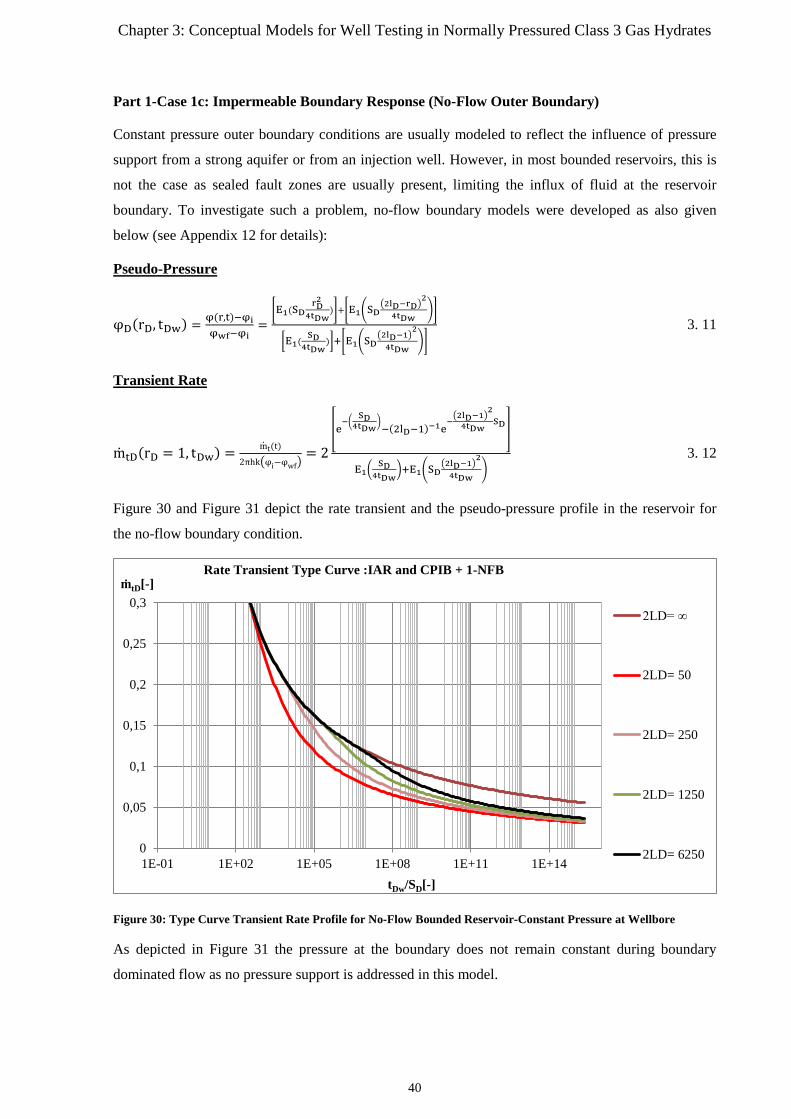
Chapter 3: Conceptual Models for Well Testing in Normally Pressured Class 3 Gas Hydrates
Part 1-Case 1c: Impermeable Boundary Response (No-Flow Outer Boundary)
Constant pressure outer boundary conditions are usually modeled to reflect the influence of pressure
support from a strong aquifer or from an injection well. However, in most bounded reservoirs, this is
not the case as sealed fault zones are usually present, limiting the influx of fluid at the reservoir
boundary. To investigate such a problem, no-flow boundary models were developed as also given
below (see Appendix 12 for details):
Pseudo-Pressure
φD(rD, tDw) = φ(r,t)−φiφwf−φi
=�E1(SD
rD2
4tDw)�+�E1�SD
�2lD−rD�2
4tDw��
�E1(SD
4tDw)�+�E1�SD
�2lD−1�2
4tDw��
3. 11
Transient Rate
mtD(rD = 1, tDw) = mt(t)
2πhk�φi−φwf�= 2
�e−�
SD4tDw
�−(2lD−1)−1e
−�2lD−1�
2
4tDwSD�
E1�SD
4tDw�+E1�SD
�2lD−1�2
4tDw�
3. 12
Figure 30 and Figure 31 depict the rate transient and the pseudo-pressure profile in the reservoir for
the no-flow boundary condition.
Figure 30: Type Curve Transient Rate Profile for No-Flow Bounded Reservoir-Constant Pressure at Wellbore
As depicted in Figure 31 the pressure at the boundary does not remain constant during boundary
dominated flow as no pressure support is addressed in this model.
0
0,05
0,1
0,15
0,2
0,25
0,3
1E-01 1E+02 1E+05 1E+08 1E+11 1E+14
ṁtD[-]
tDw/SD[-]
Rate Transient Type Curve :IAR and CPIB + 1-NFB
2LD= ∞
2LD= 50
2LD= 250
2LD= 1250
2LD= 6250
40
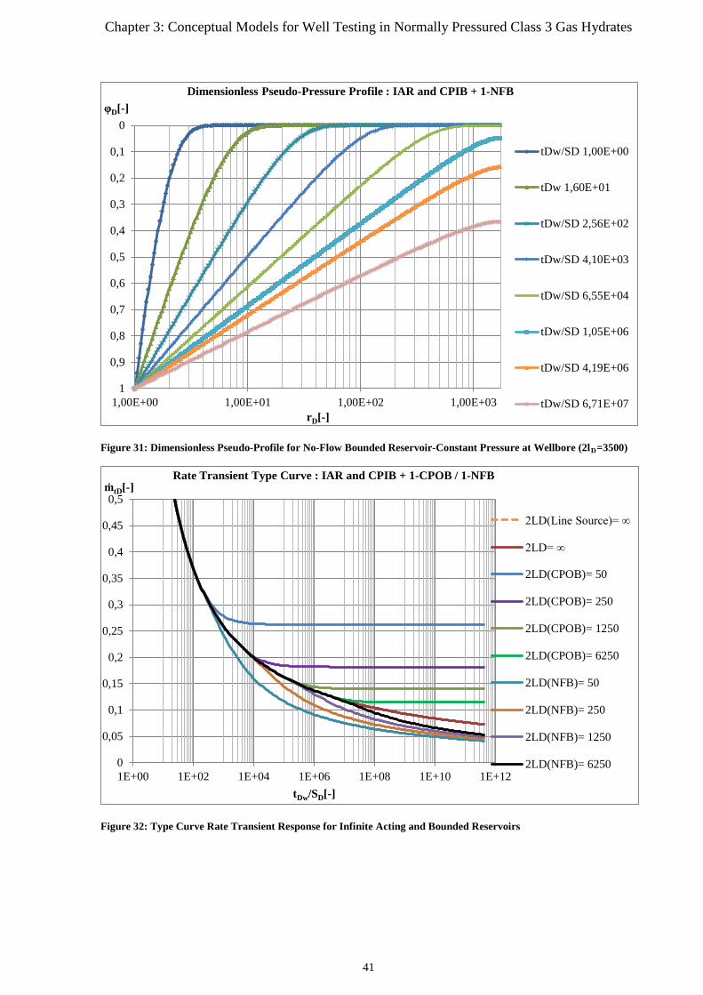
Chapter 3: Conceptual Models for Well Testing in Normally Pressured Class 3 Gas Hydrates
Figure 31: Dimensionless Pseudo-Profile for No-Flow Bounded Reservoir-Constant Pressure at Wellbore (2lD=3500)
Figure 32: Type Curve Rate Transient Response for Infinite Acting and Bounded Reservoirs
0
0,1
0,2
0,3
0,4
0,5
0,6
0,7
0,8
0,9
11,00E+00 1,00E+01 1,00E+02 1,00E+03
φD[-]
rD[-]
Dimensionless Pseudo-Pressure Profile : IAR and CPIB + 1-NFB
tDw/SD 1,00E+00
tDw 1,60E+01
tDw/SD 2,56E+02
tDw/SD 4,10E+03
tDw/SD 6,55E+04
tDw/SD 1,05E+06
tDw/SD 4,19E+06
tDw/SD 6,71E+07
0
0,05
0,1
0,15
0,2
0,25
0,3
0,35
0,4
0,45
0,5
1E+00 1E+02 1E+04 1E+06 1E+08 1E+10 1E+12
ṁtD[-]
tDw/SD[-]
Rate Transient Type Curve : IAR and CPIB + 1-CPOB / 1-NFB
2LD(Line Source)= ∞
2LD= ∞
2LD(CPOB)= 50
2LD(CPOB)= 250
2LD(CPOB)= 1250
2LD(CPOB)= 6250
2LD(NFB)= 50
2LD(NFB)= 250
2LD(NFB)= 1250
2LD(NFB)= 6250
41
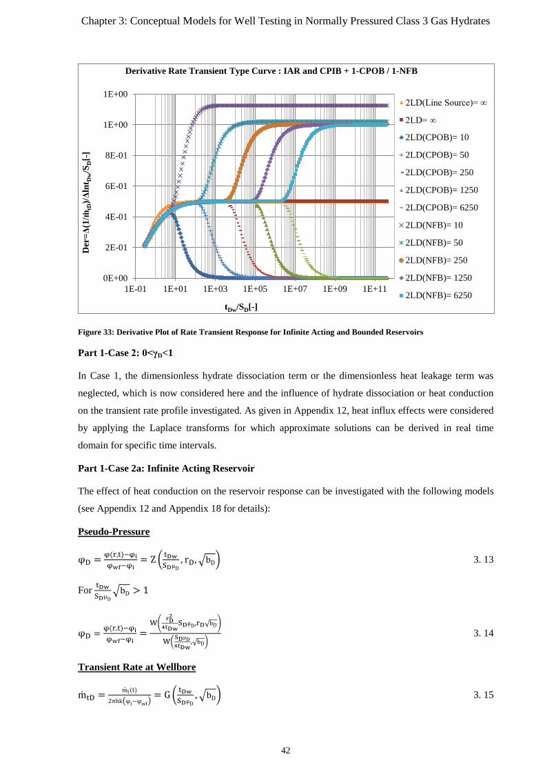
Chapter 3: Conceptual Models for Well Testing in Normally Pressured Class 3 Gas Hydrates
Figure 33: Derivative Plot of Rate Transient Response for Infinite Acting and Bounded Reservoirs
Part 1-Case 2: 0<γD<1
In Case 1, the dimensionless hydrate dissociation term or the dimensionless heat leakage term was
neglected, which is now considered here and the influence of hydrate dissociation or heat conduction
on the transient rate profile investigated. As given in Appendix 12, heat influx effects were considered
by applying the Laplace transforms for which approximate solutions can be derived in real time
domain for specific time intervals.
Part 1-Case 2a: Infinite Acting Reservoir
The effect of heat conduction on the reservoir response can be investigated with the following models
(see Appendix 12 and Appendix 18 for details):
Pseudo-Pressure
φD = φ(r,t)−φiφwf−φi
= Z � tDwSDµD
, rD,�bD� 3. 13
For tDwSDµD
�bD > 1
φD = φ(r,t)−φiφwf−φi
=W�
rD2
4tDwSDµD,rD√bD�
W�SDµD4tDw
,√bD� 3. 14
Transient Rate at Wellbore
mtD = mt(t)
2πhk�φi−φwf�= G � tDw
SDµD,�bD� 3. 15
0E+00
2E-01
4E-01
6E-01
8E-01
1E+00
1E+00
1E-01 1E+01 1E+03 1E+05 1E+07 1E+09 1E+11
Der
=Δ(1
/ṁtD
)/Δln
t Dw/S
D[-
]
tDw/SD[-]
Derivative Rate Transient Type Curve : IAR and CPIB + 1-CPOB / 1-NFB
2LD(Line Source)= ∞
2LD= ∞
2LD(CPOB)= 10
2LD(CPOB)= 50
2LD(CPOB)= 250
2LD(CPOB)= 1250
2LD(CPOB)= 6250
2LD(NFB)= 10
2LD(NFB)= 50
2LD(NFB)= 250
2LD(NFB)= 1250
2LD(NFB)= 6250
42
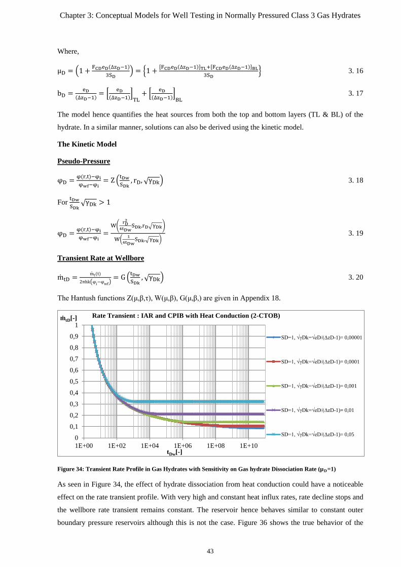
Chapter 3: Conceptual Models for Well Testing in Normally Pressured Class 3 Gas Hydrates
Where,
µD = �1 + FCDeD(∆zD−1)3SD
� = �1 + [FCDeD(∆zD−1)]TL+[FCDeD(∆zD−1)]BL3SD
� 3. 16
bD = eD(∆zD−1) = � eD
(∆zD−1)�TL+ � eD
(∆zD−1)�BL 3. 17
The model hence quantifies the heat sources from both the top and bottom layers (TL & BL) of the
hydrate. In a similar manner, solutions can also be derived using the kinetic model.
The Kinetic Model
Pseudo-Pressure
φD = φ(r,t)−φiφwf−φi
= Z �tDwSDk
, rD,√γDk� 3. 18
For tDwSDk √γDk > 1
φD = φ(r,t)−φiφwf−φi
=W�
rD2
4tDwSDk,rD�γDk�
W� 14tDw
SDk,�γDk� 3. 19
Transient Rate at Wellbore
mtD = mt(t)
2πhk�φi−φwf�= G �tDw
SDk,√γDk� 3. 20
The Hantush functions Z(μ,β,τ), W(μ,β), G(μ,β,) are given in Appendix 18.
Figure 34: Transient Rate Profile in Gas Hydrates with Sensitivity on Gas hydrate Dissociation Rate (µD=1)
As seen in Figure 34, the effect of hydrate dissociation from heat conduction could have a noticeable
effect on the rate transient profile. With very high and constant heat influx rates, rate decline stops and
the wellbore rate transient remains constant. The reservoir hence behaves similar to constant outer
boundary pressure reservoirs although this is not the case. Figure 36 shows the true behavior of the
0
0,1
0,2
0,3
0,4
0,5
0,6
0,7
0,8
0,9
1
1E+00 1E+02 1E+04 1E+06 1E+08 1E+10
ṁtD[-]
tDw[-]
Rate Transient : IAR and CPIB with Heat Conduction (2-CTOB)
SD=1, √γDk=√eD/(ΔzD-1)= 0,00001
SD=1, √γDk=√eD/(ΔzD-1)= 0,0001
SD=1, √γDk=√eD/(ΔzD-1)= 0,001
SD=1, √γDk=√eD/(ΔzD-1)= 0,01
SD=1, √γDk=√eD/(ΔzD-1)= 0,05
43

Chapter 3: Conceptual Models for Well Testing in Normally Pressured Class 3 Gas Hydrates
constant pressure outer boundary case. Here it is noticeable that the boundary dominated effects
commingle with hydrate dissociation effects as a distinction between the effects of high dissociation
rates and boundary dominated flow are difficult to differentiate. However, the models depicted in the
diagrams are reservoir responses based on the conceptual model and do not show the decrease in
hydrate saturation due to dissociation. Hence in real data analysis, provided the hydrate saturation is
very significant compared to the fluid phases and the dissociation rate is slow, boundary dominated
flow can be identified. The type curve is once more used and the rate transient takes the form:
Figure 35: Type Curve Transient Rate Profile in Bounded Reservoirs with Constant Outer Pressure
Part 1-Case 2b: Constant Pressure Outer Boundary Reservoirs
Rate Transient Approximate Solution
mtD = mt(t)
2πhk�φi−φwf�≈ 2
W�SDµD4tDw
,√bD�−W�SDµD(2lD−1)2
4tDw,(2lD−1)√bD�
3. 21
00,05
0,10,15
0,20,25
0,30,35
0,40,45
0,5
1E-02 1E+00 1E+02 1E+04 1E+06 1E+08 1E+10
ṁtD[-]
tDw/µDSD [-]
Rate Transient Type Curve: IAR and CPIB with Heat Conduction (2-CTOB)
√γDk=√eD/(ΔzD-1) 0,0001
√γDk=√eD/(ΔzD-1) 0,0005
√γDk=√eD/(ΔzD-1) 0,0025
√γDk=√eD/(ΔzD-1) 0,0125
√γDk=√eD/(ΔzD-1) 0,0625
44
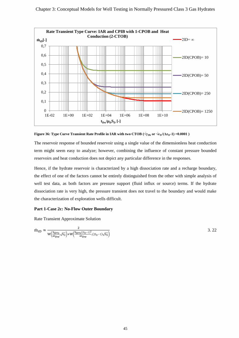
Chapter 3: Conceptual Models for Well Testing in Normally Pressured Class 3 Gas Hydrates
Figure 36: Type Curve Transient Rate Profile in IAR with two CTOB (√γDk or √eD/(ΔzD-1) =0.0001 )
The reservoir response of bounded reservoir using a single value of the dimensionless heat conduction
term might seem easy to analyze; however, combining the influence of constant pressure bounded
reservoirs and heat conduction does not depict any particular difference in the responses.
Hence, if the hydrate reservoir is characterized by a high dissociation rate and a recharge boundary,
the effect of one of the factors cannot be entirely distinguished from the other with simple analysis of
well test data, as both factors are pressure support (fluid influx or source) terms. If the hydrate
dissociation rate is very high, the pressure transient does not travel to the boundary and would make
the characterization of exploration wells difficult.
Part 1-Case 2c: No-Flow Outer Boundary
Rate Transient Approximate Solution
mtD ≈2
W�SDµD4tDw
,√bD�+W�SDµD(2lD−1)2
4tDw,(2lD−1)√bD�
3. 22
0
0,1
0,2
0,3
0,4
0,5
0,6
0,7
1E-02 1E+00 1E+02 1E+04 1E+06 1E+08 1E+10
ṁtD[-]
tDw/µDSD [-]
Rate Transient Type Curve: IAR and CPIB with 1-CPOB and Heat Conduction (2-CTOB)
2lD= ∞
2lD(CPOB)= 10
2lD(CPOB)= 50
2lD(CPOB)= 250
2lD(CPOB)= 1250
45
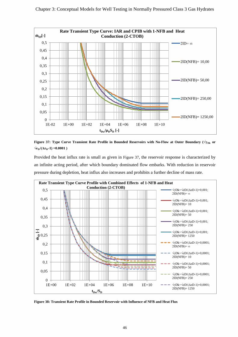
Chapter 3: Conceptual Models for Well Testing in Normally Pressured Class 3 Gas Hydrates
Figure 37: Type Curve Transient Rate Profile in Bounded Reservoirs with No-Flow at Outer Boundary (√γDk or
√eD/(ΔzD-1) =0.0001 )
Provided the heat influx rate is small as given in Figure 37, the reservoir response is characterized by
an infinite acting period, after which boundary dominated flow embarks. With reduction in reservoir
pressure during depletion, heat influx also increases and prohibits a further decline of mass rate.
Figure 38: Transient Rate Profile in Bounded Reservoir with Influence of NFB and Heat Flux
0
0,05
0,1
0,15
0,2
0,25
0,3
0,35
0,4
0,45
0,5
1E-02 1E+00 1E+02 1E+04 1E+06 1E+08 1E+10
ṁtD[-]
tDw/µDSD [-]
Rate Transient Type Curve: IAR and CPIB with 1-NFB and Heat Conduction (2-CTOB)
2lD= ∞
2lD(NFB)= 10,00
2lD(NFB)= 50,00
2lD(NFB)= 250,00
2lD(NFB)= 1250,00
0
0,05
0,1
0,15
0,2
0,25
0,3
0,35
0,4
0,45
0,5
1E+00 1E+02 1E+04 1E+06 1E+08 1E+10
ṁtD
[-]
tDw/SD
Rate Transient Type Curve Profile with Combined Effects of 1-NFB and Heat Conduction (2-CTOB)
√γDk=√eD/(ΔzD-1)=0,001; 2lD(NFB)= ∞
√γDk=√eD/(ΔzD-1)=0,001; 2lD(NFB)= 10
√γDk=√eD/(ΔzD-1)=0,001; 2lD(NFB)= 50
√γDk=√eD/(ΔzD-1)=0,001; 2lD(NFB)= 250
√γDk=√eD/(ΔzD-1)=0,001; 2lD(NFB)= 1250
√γDk=√eD/(ΔzD-1)=0,0001; 2lD(NFB)= ∞
√γDk=√eD/(ΔzD-1)=0,0001; 2lD(NFB)= 10
√γDk=√eD/(ΔzD-1)=0,0001; 2lD(NFB)= 50
√γDk=√eD/(ΔzD-1)=0,0001; 2lD(NFB)= 250
√γDk=√eD/(ΔzD-1)=0,0001; 2lD(NFB)= 1250
46
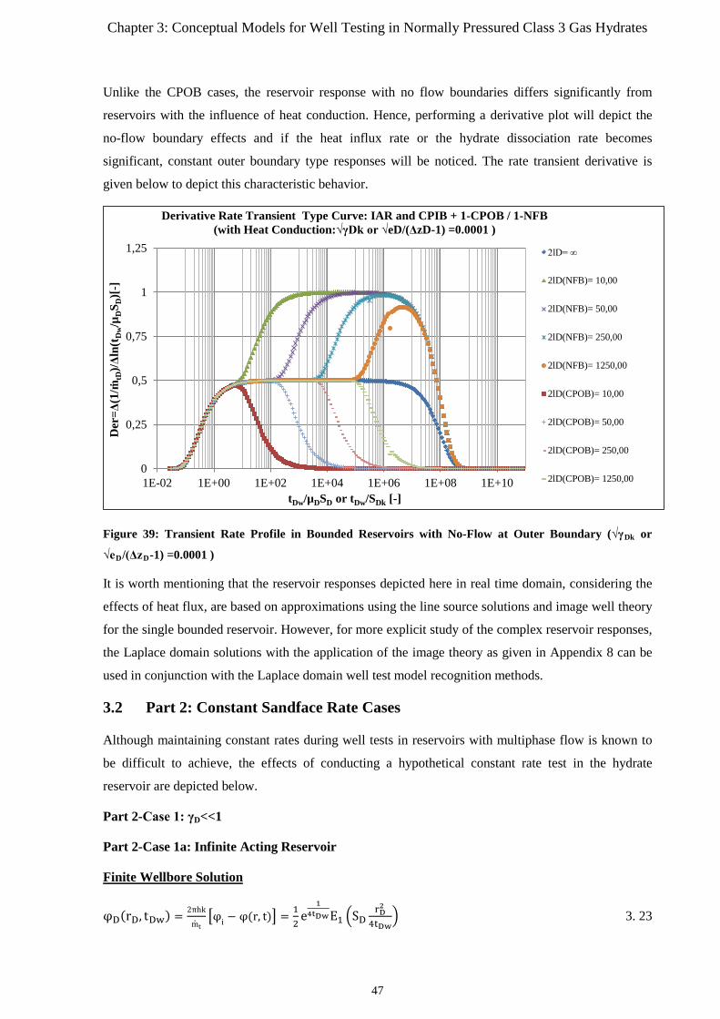
Chapter 3: Conceptual Models for Well Testing in Normally Pressured Class 3 Gas Hydrates
Unlike the CPOB cases, the reservoir response with no flow boundaries differs significantly from
reservoirs with the influence of heat conduction. Hence, performing a derivative plot will depict the
no-flow boundary effects and if the heat influx rate or the hydrate dissociation rate becomes
significant, constant outer boundary type responses will be noticed. The rate transient derivative is
given below to depict this characteristic behavior.
Figure 39: Transient Rate Profile in Bounded Reservoirs with No-Flow at Outer Boundary (√γDk or
√eD/(ΔzD-1) =0.0001 )
It is worth mentioning that the reservoir responses depicted here in real time domain, considering the
effects of heat flux, are based on approximations using the line source solutions and image well theory
for the single bounded reservoir. However, for more explicit study of the complex reservoir responses,
the Laplace domain solutions with the application of the image theory as given in Appendix 8 can be
used in conjunction with the Laplace domain well test model recognition methods.
3.2 Part 2: Constant Sandface Rate Cases
Although maintaining constant rates during well tests in reservoirs with multiphase flow is known to
be difficult to achieve, the effects of conducting a hypothetical constant rate test in the hydrate
reservoir are depicted below.
Part 2-Case 1: γD<<1
Part 2-Case 1a: Infinite Acting Reservoir
Finite Wellbore Solution
φD(rD, tDw) = 2πhk
mt�φi − φ(r, t)� = 1
2e
14tDwE1 �SD
rD2
4tDw� 3. 23
0
0,25
0,5
0,75
1
1,25
1E-02 1E+00 1E+02 1E+04 1E+06 1E+08 1E+10
Der
=Δ(1
/ṁtD
)/Δln
(tD
w/µ
DS D
)[-]
tDw/µDSD or tDw/SDk [-]
Derivative Rate Transient Type Curve: IAR and CPIB + 1-CPOB / 1-NFB (with Heat Conduction:√γDk or √eD/(ΔzD-1) =0.0001 )
2lD= ∞
2lD(NFB)= 10,00
2lD(NFB)= 50,00
2lD(NFB)= 250,00
2lD(NFB)= 1250,00
2lD(CPOB)= 10,00
2lD(CPOB)= 50,00
2lD(CPOB)= 250,00
2lD(CPOB)= 1250,00
47
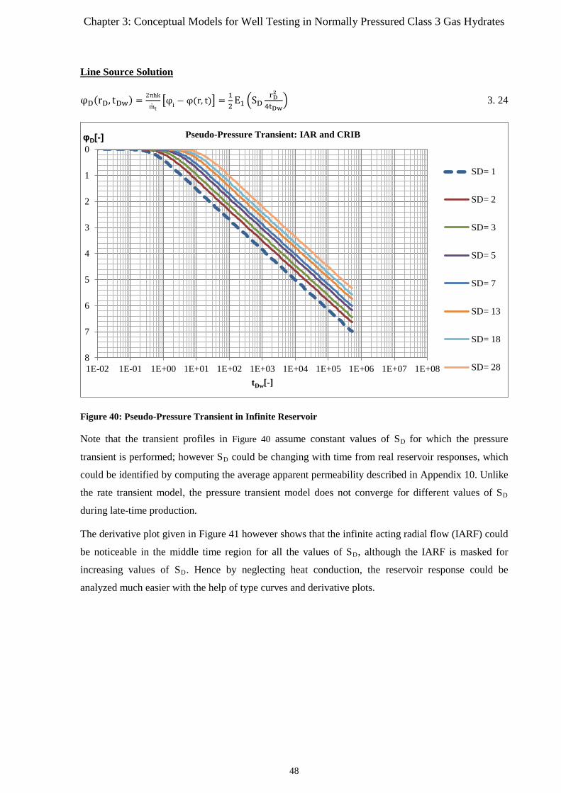
Chapter 3: Conceptual Models for Well Testing in Normally Pressured Class 3 Gas Hydrates
Line Source Solution
φD(rD, tDw) = 2πhk
mt�φi − φ(r, t)� = 1
2E1 �SD
rD2
4tDw� 3. 24
Figure 40: Pseudo-Pressure Transient in Infinite Reservoir
Note that the transient profiles in Figure 40 assume constant values of SD for which the pressure
transient is performed; however SD could be changing with time from real reservoir responses, which
could be identified by computing the average apparent permeability described in Appendix 10. Unlike
the rate transient model, the pressure transient model does not converge for different values of SD
during late-time production.
The derivative plot given in Figure 41 however shows that the infinite acting radial flow (IARF) could
be noticeable in the middle time region for all the values of SD, although the IARF is masked for
increasing values of SD. Hence by neglecting heat conduction, the reservoir response could be
analyzed much easier with the help of type curves and derivative plots.
0
1
2
3
4
5
6
7
81E-02 1E-01 1E+00 1E+01 1E+02 1E+03 1E+04 1E+05 1E+06 1E+07 1E+08
φD[-]
tDw[-]
Pseudo-Pressure Transient: IAR and CRIB
SD= 1
SD= 2
SD= 3
SD= 5
SD= 7
SD= 13
SD= 18
SD= 28
48
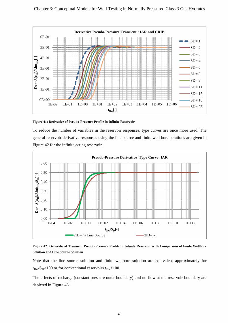
Chapter 3: Conceptual Models for Well Testing in Normally Pressured Class 3 Gas Hydrates
Figure 41: Derivative of Pseudo-Pressure Profile in Infinite Reservoir
To reduce the number of variables in the reservoir responses, type curves are once more used. The
general reservoir derivative responses using the line source and finite well bore solutions are given in
Figure 42 for the infinite acting reservoir.
Figure 42: Generalized Transient Pseudo-Pressure Profile in Infinite Reservoir with Comparison of Finite Wellbore
Solution and Line Source Solution
Note that the line source solution and finite wellbore solution are equivalent approximately for
tDw/SD>100 or for conventional reservoirs tDw>100.
The effects of recharge (constant pressure outer boundary) and no-flow at the reservoir boundary are
depicted in Figure 43.
0E+00
1E-01
2E-01
3E-01
4E-01
5E-01
6E-01
1E-02 1E-01 1E+00 1E+01 1E+02 1E+03 1E+04 1E+05 1E+06
Der
=Δ(φ
D)/Δ
lnt D
w[-
]
tDw[-]
Derivative Pseudo-Pressure Transient : IAR and CRIB
SD= 1
SD= 2
SD= 3
SD= 4
SD= 6
SD= 8
SD= 9
SD= 11
SD= 15
SD= 18
SD= 28
0,00
0,10
0,20
0,30
0,40
0,50
0,60
1E-04 1E-02 1E+00 1E+02 1E+04 1E+06 1E+08 1E+10 1E+12
Der
=Δ(φ
D)/Δ
ln(t
Dw/S
D)[
-]
tDw/SD[-]
Pseudo-Pressure Derivative Type Curve: IAR
2lD=∞ (Line Source) 2lD= ∞
49
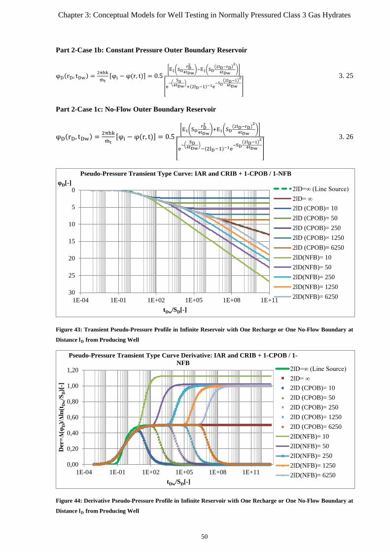
Chapter 3: Conceptual Models for Well Testing in Normally Pressured Class 3 Gas Hydrates
Part 2-Case 1b: Constant Pressure Outer Boundary Reservoir
φD(rD, tDw) = 2πhkmt
[φi − φ(r, t)] = 0.5�E1�SD
rD2
4tDw�−E1�SD
�2lD−rD�2
4tDw��
�e−�
SD4tDw
�+(2lD−1)−1e
−SD�2lD−1�
2
4tDw �
3. 25
Part 2-Case 1c: No-Flow Outer Boundary Reservoir
φD(rD, tDw) = 2πhkmt
[φi − φ(r, t)] = 0.5�E1�SD
rD2
4tDw�+E1�SD
�2lD−rD�2
4tDw��
�e−�
SD4tDw
�−(2lD−1)−1e
−SD�2lD−1�
2
4tDw �
3. 26
Figure 43: Transient Pseudo-Pressure Profile in Infinite Reservoir with One Recharge or One No-Flow Boundary at
Distance lD from Producing Well
Figure 44: Derivative Pseudo-Pressure Profile in Infinite Reservoir with One Recharge or One No-Flow Boundary at
Distance lD from Producing Well
0
5
10
15
20
25
301E-04 1E-01 1E+02 1E+05 1E+08 1E+11
φD[-]
tDw/SD[-]
Pseudo-Pressure Transient Type Curve: IAR and CRIB + 1-CPOB / 1-NFB
2lD=∞ (Line Source) 2lD= ∞ 2lD (CPOB)= 102lD (CPOB)= 502lD (CPOB)= 2502lD (CPOB)= 12502lD (CPOB)= 62502lD(NFB)= 102lD(NFB)= 502lD(NFB)= 2502lD(NFB)= 12502lD(NFB)= 6250
0,00
0,20
0,40
0,60
0,80
1,00
1,20
1E-04 1E-01 1E+02 1E+05 1E+08 1E+11
Der
=Δ(φ
D)/Δ
ln(t
Dw/S
D)[
-]
tDw/SD[-]
Pseudo-Pressure Transient Type Curve Derivative: IAR and CRIB + 1-CPOB / 1-NFB
2lD=∞ (Line Source) 2lD= ∞ 2lD (CPOB)= 102lD (CPOB)= 502lD (CPOB)= 2502lD (CPOB)= 12502lD (CPOB)= 62502lD(NFB)= 102lD(NFB)= 502lD(NFB)= 2502lD(NFB)= 12502lD(NFB)= 6250
50

Chapter 3: Conceptual Models for Well Testing in Normally Pressured Class 3 Gas Hydrates
Part 2-Case 2: 0<γD<1
Part 2-Case 2a: Infinite Acting Reservoir
The transient pseudo-pressure response considering heat conduction can be estimated with the
following models:
Early-Time Response
φD = 2πhkmt
[φi − φ(r, t)] = H �SDrD2
4tDw, rD4eD�FCD�SD
� 3. 27
Late Time Response
φD = 2πhkmt
[φi − φ(r, t)] = 12
W �rD2 SDµD4tDw
, rD�bD� 3. 28
The early and late time responses are very dependent on the thickness of the confining layers. As also
given in Appendix 12 using the Laplace domain well test model recognition, late time solution can be
conveniently used to describe the reservoir response at any production time provided the confining
layers are thin.
Kinetic Model
With the Kinetic model, no early time and late time approximations are required; yet, the line source
solution is still used. The solution to the kinetic model takes the form:
φD = 2πhkmt
[φi − φ(r, t)] = 12
W � rD2
4tDwSDk, rD√γDk� 3. 29
Figure 45 depicts the dimensionless pseudo-pressure drawdown profile in a normally pressured gas
hydrate reservoir with constant sandface rates. In the beginning, the hydrate dissociation is mainly
influenced by the heat energy stored in the reservoir and when pressure drawdown is significant at
later production times, the hydrate dissociation increases accordingly due to heat flux from
conduction. If the heat flux is constant and the saturation of hydrate is extremely large, the hydrate
dissociation would act as a strong pressure support and the reservoir responses will be similar to
constant pressure outer boundary responses as seen in Figure 43.
From well test analysis, the first slope of the semi-log plot will depict the average reservoir
permeability without the influence of heat conduction from the confining layers.
51
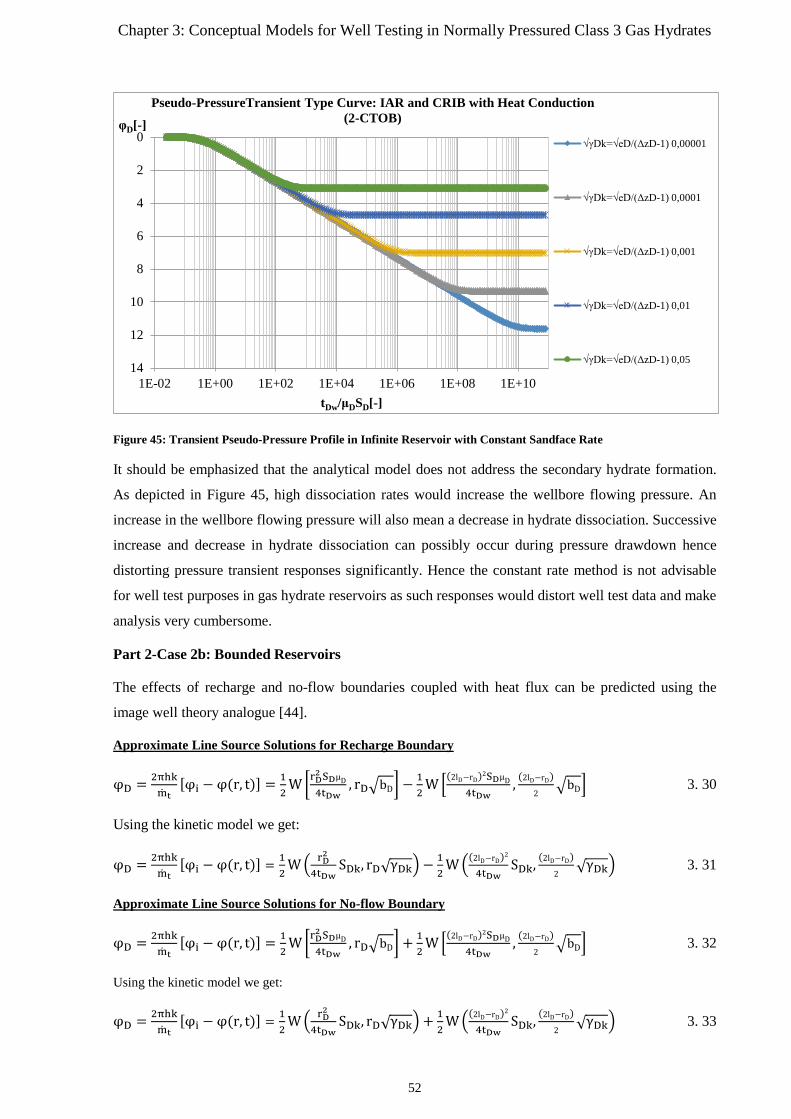
Chapter 3: Conceptual Models for Well Testing in Normally Pressured Class 3 Gas Hydrates
Figure 45: Transient Pseudo-Pressure Profile in Infinite Reservoir with Constant Sandface Rate
It should be emphasized that the analytical model does not address the secondary hydrate formation.
As depicted in Figure 45, high dissociation rates would increase the wellbore flowing pressure. An
increase in the wellbore flowing pressure will also mean a decrease in hydrate dissociation. Successive
increase and decrease in hydrate dissociation can possibly occur during pressure drawdown hence
distorting pressure transient responses significantly. Hence the constant rate method is not advisable
for well test purposes in gas hydrate reservoirs as such responses would distort well test data and make
analysis very cumbersome.
Part 2-Case 2b: Bounded Reservoirs
The effects of recharge and no-flow boundaries coupled with heat flux can be predicted using the
image well theory analogue [44].
Approximate Line Source Solutions for Recharge Boundary
φD = 2πhkmt
[φi − φ(r, t)] = 12
W �rD2 SDµD4tDw
, rD�bD� −12
W �(2lD−rD)2SDµD4tDw
, (2lD−rD)2
�bD� 3. 30
Using the kinetic model we get:
φD = 2πhkmt
[φi − φ(r, t)] = 12
W � rD2
4tDwSDk, rD√γDk� −
12
W �(2lD−rD)2
4tDwSDk, (2lD−rD)
2 √γDk� 3. 31
Approximate Line Source Solutions for No-flow Boundary
φD = 2πhkmt
[φi − φ(r, t)] = 12
W �rD2 SDµD4tDw
, rD�bD� + 12
W �(2lD−rD)2SDµD4tDw
, (2lD−rD)2
�bD� 3. 32
Using the kinetic model we get:
φD = 2πhkmt
[φi − φ(r, t)] = 12
W � rD2
4tDwSDk, rD√γDk� + 1
2W �(2lD−rD)2
4tDwSDk, (2lD−rD)
2 √γDk� 3. 33
0
2
4
6
8
10
12
141E-02 1E+00 1E+02 1E+04 1E+06 1E+08 1E+10
φD[-]
tDw/μDSD[-]
Pseudo-PressureTransient Type Curve: IAR and CRIB with Heat Conduction (2-CTOB)
√γDk=√eD/(ΔzD-1) 0,00001
√γDk=√eD/(ΔzD-1) 0,0001
√γDk=√eD/(ΔzD-1) 0,001
√γDk=√eD/(ΔzD-1) 0,01
√γDk=√eD/(ΔzD-1) 0,05
52
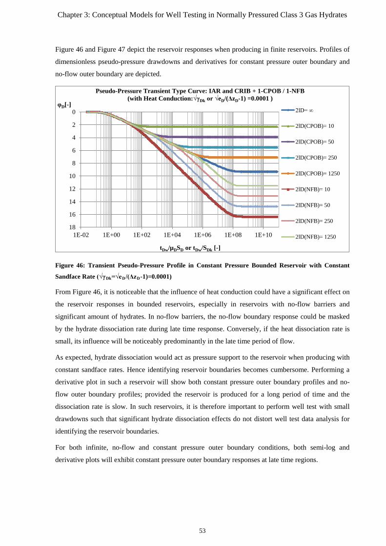
Chapter 3: Conceptual Models for Well Testing in Normally Pressured Class 3 Gas Hydrates
Figure 46 and Figure 47 depict the reservoir responses when producing in finite reservoirs. Profiles of
dimensionless pseudo-pressure drawdowns and derivatives for constant pressure outer boundary and
no-flow outer boundary are depicted.
Figure 46: Transient Pseudo-Pressure Profile in Constant Pressure Bounded Reservoir with Constant
Sandface Rate (√γDk=√eD/(ΔzD-1)=0.0001)
From Figure 46, it is noticeable that the influence of heat conduction could have a significant effect on
the reservoir responses in bounded reservoirs, especially in reservoirs with no-flow barriers and
significant amount of hydrates. In no-flow barriers, the no-flow boundary response could be masked
by the hydrate dissociation rate during late time response. Conversely, if the heat dissociation rate is
small, its influence will be noticeably predominantly in the late time period of flow.
As expected, hydrate dissociation would act as pressure support to the reservoir when producing with
constant sandface rates. Hence identifying reservoir boundaries becomes cumbersome. Performing a
derivative plot in such a reservoir will show both constant pressure outer boundary profiles and no-
flow outer boundary profiles; provided the reservoir is produced for a long period of time and the
dissociation rate is slow. In such reservoirs, it is therefore important to perform well test with small
drawdowns such that significant hydrate dissociation effects do not distort well test data analysis for
identifying the reservoir boundaries.
For both infinite, no-flow and constant pressure outer boundary conditions, both semi-log and
derivative plots will exhibit constant pressure outer boundary responses at late time regions.
0
2
4
6
8
10
12
14
16
181E-02 1E+00 1E+02 1E+04 1E+06 1E+08 1E+10
φD[-]
tDw/µDSD or tDw/SDk [-]
Pseudo-Pressure Transient Type Curve: IAR and CRIB + 1-CPOB / 1-NFB (with Heat Conduction:√γDk or √eD/(ΔzD-1) =0.0001 )
2lD= ∞
2lD(CPOB)= 10
2lD(CPOB)= 50
2lD(CPOB)= 250
2lD(CPOB)= 1250
2lD(NFB)= 10
2lD(NFB)= 50
2lD(NFB)= 250
2lD(NFB)= 1250
53
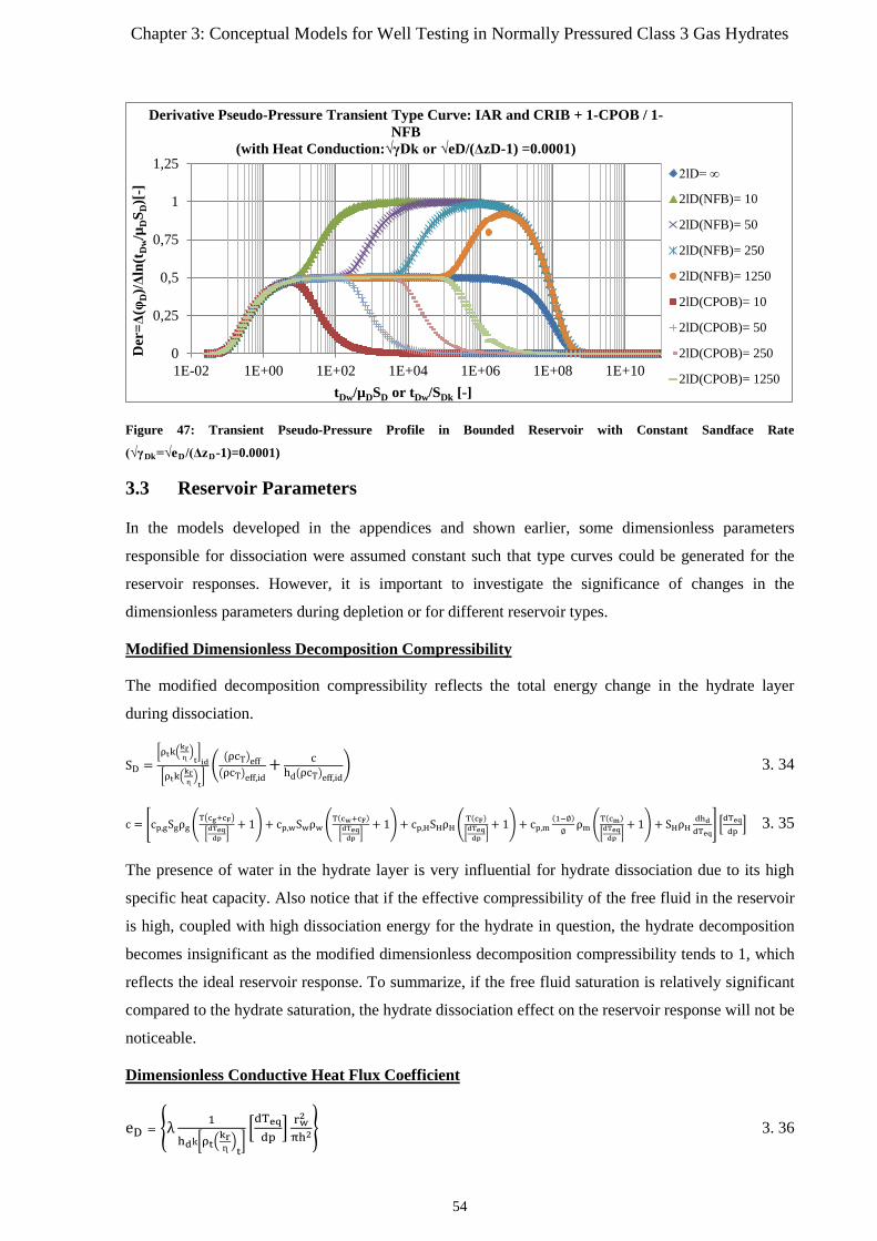
Chapter 3: Conceptual Models for Well Testing in Normally Pressured Class 3 Gas Hydrates
Figure 47: Transient Pseudo-Pressure Profile in Bounded Reservoir with Constant Sandface Rate
(√γDk=√eD/(ΔzD-1)=0.0001)
3.3 Reservoir Parameters
In the models developed in the appendices and shown earlier, some dimensionless parameters
responsible for dissociation were assumed constant such that type curves could be generated for the
reservoir responses. However, it is important to investigate the significance of changes in the
dimensionless parameters during depletion or for different reservoir types.
Modified Dimensionless Decomposition Compressibility
The modified decomposition compressibility reflects the total energy change in the hydrate layer
during dissociation.
SD =�ρtk�
krɳ �t
�id
�ρtk�krɳ �t
��
�ρcT�eff�ρcT�eff,id
+ chd�ρcT�eff,id
� 3. 34
c = �cp,gSgρg �T�cg+cF�
�dTeqdp �
+ 1� + cp,wSwρw �T(cw+cF)
�dTeqdp �
+ 1� + cp,HSHρH �T(cF)
�dTeqdp �
+ 1� + cp,m(1−∅)∅
ρm �T(cm)
�dTeqdp �
+ 1� + SHρHdhddTeq
� �dTeqdp
� 3. 35
The presence of water in the hydrate layer is very influential for hydrate dissociation due to its high
specific heat capacity. Also notice that if the effective compressibility of the free fluid in the reservoir
is high, coupled with high dissociation energy for the hydrate in question, the hydrate decomposition
becomes insignificant as the modified dimensionless decomposition compressibility tends to 1, which
reflects the ideal reservoir response. To summarize, if the free fluid saturation is relatively significant
compared to the hydrate saturation, the hydrate dissociation effect on the reservoir response will not be
noticeable.
Dimensionless Conductive Heat Flux Coefficient
eD = �λ 1
hdk�ρt�krɳ �t
��dTeqdp
� rw2
πh2� 3. 36
0
0,25
0,5
0,75
1
1,25
1E-02 1E+00 1E+02 1E+04 1E+06 1E+08 1E+10
Der
=Δ(φ
D)/Δ
ln(t
Dw/µ
DS D
)[-]
tDw/µDSD or tDw/SDk [-]
Derivative Pseudo-Pressure Transient Type Curve: IAR and CRIB + 1-CPOB / 1-NFB
(with Heat Conduction:√γDk or √eD/(ΔzD-1) =0.0001)
2lD= ∞
2lD(NFB)= 10
2lD(NFB)= 50
2lD(NFB)= 250
2lD(NFB)= 1250
2lD(CPOB)= 10
2lD(CPOB)= 50
2lD(CPOB)= 250
2lD(CPOB)= 1250
54
Chapter 3: Conceptual Models for Well Testing in Normally Pressured Class 3 Gas Hydrates
The amount of heat flux into the hydrate layer for dissociation is highly dependent on the interlayer
heat flux coefficient given above. Recognizing the very little changes in the heat conductivity of
formation rocks, we can conclude that the influence of heat conduction diminishes with increasing
mobility of the free fluid layer and increasing thickness of the hydrate layer.
Dimensionless Interlayer Heat Flux Coefficient
bD = eD(∆zD−1)
3. 37
∆zD = ∆z
�h2�=
��h2�+hconfining layer�
�h2� 3. 38
From the definition of the dimensionless interlayer heat influx coefficient, the smaller the thickness of
the confining layer coupled with the constant outer temperature imposed on this layer, the higher the
heat influx rate. This implies even with a small value of the dimensionless heat flux coefficient, the
value of the dimensionless interlayer coefficient could increase significantly for thin confining layers.
Dimensionless Interlayer Heat Flux Compressibility
SDµD = �SD + FCDeD(∆zD−1)3
� 3. 39
FCD = h2
4
�ρcp�effλ
�rw2 ��ρw∅cT,w�+�ρg∅cT,g��
k�ρt�krɳ �t
��i
3. 40
eD = �λ 1
hdk�ρt�krɳ �t
��dTeqdp
� rw2
πh2� 3. 41
SDµD = SD + �(∆zD−1)3
�dTeqdp
��ρcp�eff
4hdk�ρt�krɳ �t
�π�rw
4 ∅��ρwcT,w�+�ρgcT,g��
k�ρt�krɳ �t
��i
� 3. 42
Similarly, hydrate reservoirs with high permeabilities and high dissociation energies will have
negligible influence from heat conduction as the second term on the right hand side of the equation
above becomes insignificant especially in the early time period of production.
3.4 Rate Transient Analysis in Normally Pressured Gas Hydrate Reservoirs
Pressure and rate transient data provide a good source of understanding reservoir behavior under
different production scenarios. From test data we strive at obtaining vital reservoir parameters such as
the permeability. However, the multiphase well test model developed earlier uses total mass rates of
the whole system. Moreover, the multiphase pseudo-pressure used for linearization should be
retransformed for well test analysis purposes. Other approaches still exist in analyzing two phase well
test data such as [53], [62].
55
Chapter 3: Conceptual Models for Well Testing in Normally Pressured Class 3 Gas Hydrates
Rate Transient Analysis
The rate transient models developed in this work assumed constant multiphase pseudo pressure as a
prerequisite for applying future superposition techniques. Hence, the methods of analysis developed
hereafter address the constant multiphase pseudo-pressure. The next challenge lays in the derivation of
the rate transient parameters of the different phases in the system. We first address the mass balance
model as follows:
Multiphase
The dimensionless flow rate:
mtD = ρt,stQt,st(t)
2πhk∫ρt�krɳ �t
dp= mt
2πhk∫ρt�krɳ �t
dp 3. 43
mt = mtD �2πhk∫ρt �krɳ�t
dp� = mtD[2πhk∫ ft(p)dp] 3. 44
The fractional mass flow:
mt = mg,t + mw,t 3. 45
mtmt
= mg,t
mt+ mw,t
mt= fm,g + fm,w = fm,t 3. 46
Gas Phase
mg,t
mt=
∫�ρgkrg∗
ɳg�dp
∫ρt�krɳ �t
dp= ∫ fg(p)dp
∫ ft(p)dp= fm,g 3. 47
k∫ fg(p)dp = mg,t
mtk∫ ft(p)dp = fm,gk∫ ft(p)dp 3. 48
With the introduction of the pressure dependent pseudo-relative permeability [krg*(p)] given in
Appendix 10, the equation above takes the form:
kkrg∗ (p)∫ρgɳg
dp = Qg,stρg,st
mtk∫ ft(p)dp 3. 49
kkrg∗ (p) =[φPI(t)]g
mt[k∫ ft(p)dp] 3. 50
Where,
[φPI(t)]𝑔𝑔 =Qg,stρg,st
∫ρgɳg
dp=
Qg,st
∫ 1Bgɳg
dp
The pseudo-pressure normalized rate (pseudo productivity index) representation above gives a
relationship between the transient flow rate and the pseudo-pressure which is constant in this case for
constant wellbore pressure tests.
56

Chapter 3: Conceptual Models for Well Testing in Normally Pressured Class 3 Gas Hydrates
Water Phase
Similarly, the effective permeability of the water phase could be given thus:
kkrw∗ (p) = [φPI(t)]wmt
[k∫ ft(p)dp] 3. 51
Rate transient analyses should therefore be performed for the total system response, which is the
linearized form of the reservoir response. From the derived parameters, the effective permeability of
the different phases can be derived from the solutions derived for the dimensionless multiphase
transient mass rate in Appendix 12.
3.4.1 Semi-log Analysis
To derive the reservoir parameters, it is essential to define a range for which IARF is easily noticeable
such that semi-log analysis can be performed. From the models depicted earlier for the reservoir
responses, the following range can be used:
Range: 10²<tDw/μDSD<104 and �eD
(∆zD−1) < 0.01
The numerical approximation given by [63] for rate transient solution in Appendix 12 can be
simplified to:
mtD = 1
0.48465ln� tDwSDµD�+0.64757
3. 52
1mt
= 12πh[k∫ ft(p)dp] �0.48465ln � tDw
SDµD� + 0.64757� 3. 53
By expanding the dimensionless time, relating the gas density with the formation volume factor and
considering the dimensionless compressibility-mobility, the above equation can be written in terms of
real time:
1mt
= 1.11612πh[k∫ ft(p)dp] �logt + log � k
∅rw2ft(pi)β(pi)
� − log�SDµD� + 0.58018� 3. 54
Where,
ft(pi)β(pi)
=ρt,i�
krɳ �t,i
��ρw,icT,w,i�+�ρg,icT,g,i�� 3. 55
Semi-log Plot
1mt
𝑉𝑉𝑉𝑉𝑟𝑟𝑉𝑉𝑉𝑉𝑉𝑉 𝑡𝑡
A semi-log plot of the reciprocal total mass rate versus the time should give a straight line during
infinite acting flow, provided the changes in the dimensionless dissociation terms (SDμD) with
pressure are negligible. The gradient of the line can hence be used to estimate the effective
permeability of the flowing phases.
57
Chapter 3: Conceptual Models for Well Testing in Normally Pressured Class 3 Gas Hydrates
The gradient of the semi-log plot:
mlog = 1.11612πh[k∫ ft(p)dp] 3. 56
�k� ft(p)dp� =1.11612πhmlog
Effective gas permeability at IARF
kkrg∗ (p) = kg∗(p) =[φPI(t)]g
mt[k∫ ft(p)dp] =
[φPI(t)]gmt
1.11612πhmlog
3. 57
Dimensionless Dissociation Terms (IARF)
Applying the damage skin approach for well test analysis we get an approximation of the dissociation
terms for the hydrate layer.
(SDµD)avg = �SD + FCDeD(∆zD−1)3
�avg
≈ exp �−0.434 �� 1mt�t=1s
mlog− log � k
∅rw2ft(pi)β(pi)
∗ 100.58018��� 3. 58
It is worth mentioning that the above method of analysis just approximately quantifies the degree of
hydrate dissociation.
Note that if heat conduction influence is negligible, the following are valid:
10²<tDw/SD and �eD
(∆zD−1) ≪ 1
(SDµD)avg ≈ SD,avg ≈ exp �−0.434 �� 1mt�𝑡𝑡=1𝑉𝑉
mlog− log � k
∅rw2ft�pi�β(pi)
∗ 100.58018��� 3. 59
The rate transient solution can be simplified to:
mtD = 1
0.48465ln�tDwSD�+0.64757
3. 60
The same procedures applied earlier are also applicable. It should be highlighted that some constant
pressure tests are conducted by adjusting the surface pressure to constant values for example at
separator point. From pressure profile calculations in wellbores, a constant wellhead pressure and
changing flow rates will imply the flowing downhole pressure will constantly be changing. With this
regard, it is vital to modify the rate transient equation for such a system and this could be done by
applying the superposition principle for multi-pressure solutions [64]. This is though cumbersome for
multiphase systems and will not be addressed in this work. To avoid complicated analyses, pump
installations for depressurizing the hydrate layer should be as close to the reservoir producing layer as
possible.
58
Chapter 3: Conceptual Models for Well Testing in Normally Pressured Class 3 Gas Hydrates
3.4.2 Rate Derivative Analysis
The derivative plot is principally used for diagnosis of the reservoir behavior and for a better view of
the different flow regimes and boundary responses. However, the works of Tiab [ [57], [65], [66] ]
have shown that the derivative analysis can be used in deriving reservoir parameter. Nonetheless, this
will not be addressed in this work and just derivative responses are highlighted.
The derivative for RTA is given by:
d� 1mt�
dlnt= 0.5
2πh[k∫ ft(p)dp] = Der 3. 61
The log-log derivative plot is given by:
d� 1mt
)�
dlnt=
d� 1mt�
dtt = 0.5
2πh[k∫ ft(p)dp])= Der 3. 62
log �d� 1
mt�
dtt� = log � 0.5
2πh[k∫ ft(p)dp])� 3. 63
Plot
log �d� 1
mt�
dtt� vs logt 3. 64
If the derivative is time independent, the log-log plot will remain constant during IARF.
kg,avg∗ (p) =
[φPI(t)]gmt
[k∫ ft(p)dp] =[φPI(t)]g
mt
0.52πhDer
3. 65
Characteristics of Type Curve Derivatives
Early Time Region
No skin response from model.
IARF
d� 1mtD
�
d�ln� tDwµDSD
��= 0.5 3. 66
Boundary dominated Flow with 1-NFB and negligible heat influx
𝑈𝑈� 1mtD
�
𝑈𝑈�ln� tDw𝜇𝜇𝐷𝐷SD
��= 1 3. 67
Boundary dominated Flow with 1-CPOB
𝑈𝑈� 1mtD
�
𝑈𝑈�ln� tDw𝜇𝜇𝐷𝐷SD
��= 0 3. 68
59
Chapter 3: Conceptual Models for Well Testing in Normally Pressured Class 3 Gas Hydrates
Boundary dominated Flow with 1-NFB or 1-CPOB and high heat influx
𝑈𝑈� 1mtD
�
𝑈𝑈�ln� tDw𝜇𝜇𝐷𝐷SD
��= 0 3. 69
3.4.3 Identifying Reservoir Boundaries (Heat conduction effects are negligible)
mtD(rD = 1, tDw) = mt(t)
2πhk�φi−φwf�= 2
�e−�
SD4tDw
�±(2lD−1)−1e
−�2lD−1�
2
4tDwSD�
E1�SD
4tDw�∓E1�SD
�2lD−1�2
4tDw�
3. 70
mtD(rD = 1, tDw) = mt(t)
2πhk�φi−φwf�= 2
�e−(x1)± e−x2�2lD−1�
�
E1(x1)∓E1(x2) 3. 71
Boundary dominated flow is perceived when the Ei-function containing the boundary term becomes
noticeable. This is achieved approximately for values x2 ≤701.828 (where E1(x2)=2.2548E-308) or for
more practical purposes (which could also be noticed from a derivative plot) at x2=4 (where
E1(x2)=3.78E-03). The second value of x2 will be considered which actually denotes the transition
point, much noticeable from a derivative plot; nevertheless, when using the semi-log plots, lower
values can be used such as 1.785 [67], which has been described by the authors as the point whereby
the IARF gradient intersects the boundary dominated flow gradient. With this said, the value of the
distance to the boundary can be estimated thus:
SD(2lD−1)2
4tDw,t= 4 3. 72
𝑙𝑙𝐷𝐷 = 𝑙𝑙rw
= �2 ∗ �tDw,tfSD
� + 0.5 3. 73
𝑙𝑙 = �2 ∗ ��k∅ft(pi)β(pi)
𝑡𝑡𝑡𝑡𝑡𝑡∗ �1SD�+ 0.5rw ≈ 2 �∗ ��k∅
ft(pi)β(pi)
𝑡𝑡𝑡𝑡𝑡𝑡∗ �1SD� 3. 74
The time ttf* reflects the time at which the deviation from IARF to boundary dominated flow
immediately embarks and is best derived from the derivative plot.
Using the model given by [67] we get:
𝑙𝑙 = 0.75 ���k∅ft(pi)β(pi)
𝑡𝑡𝑡𝑡∗�1SD� 3. 75
𝑙𝑙 = 0.75rw ��tDw,fSD
� 3. 76
The time tf* reflects the time whereby the IARF gradient intersects the boundary dominated flow
gradient and is best derived from a semi-log plot. It should be noted that the intersection time is
greater than the transition time; as such, the two models should give the same value if the flowing
times are correctly deduced.
60
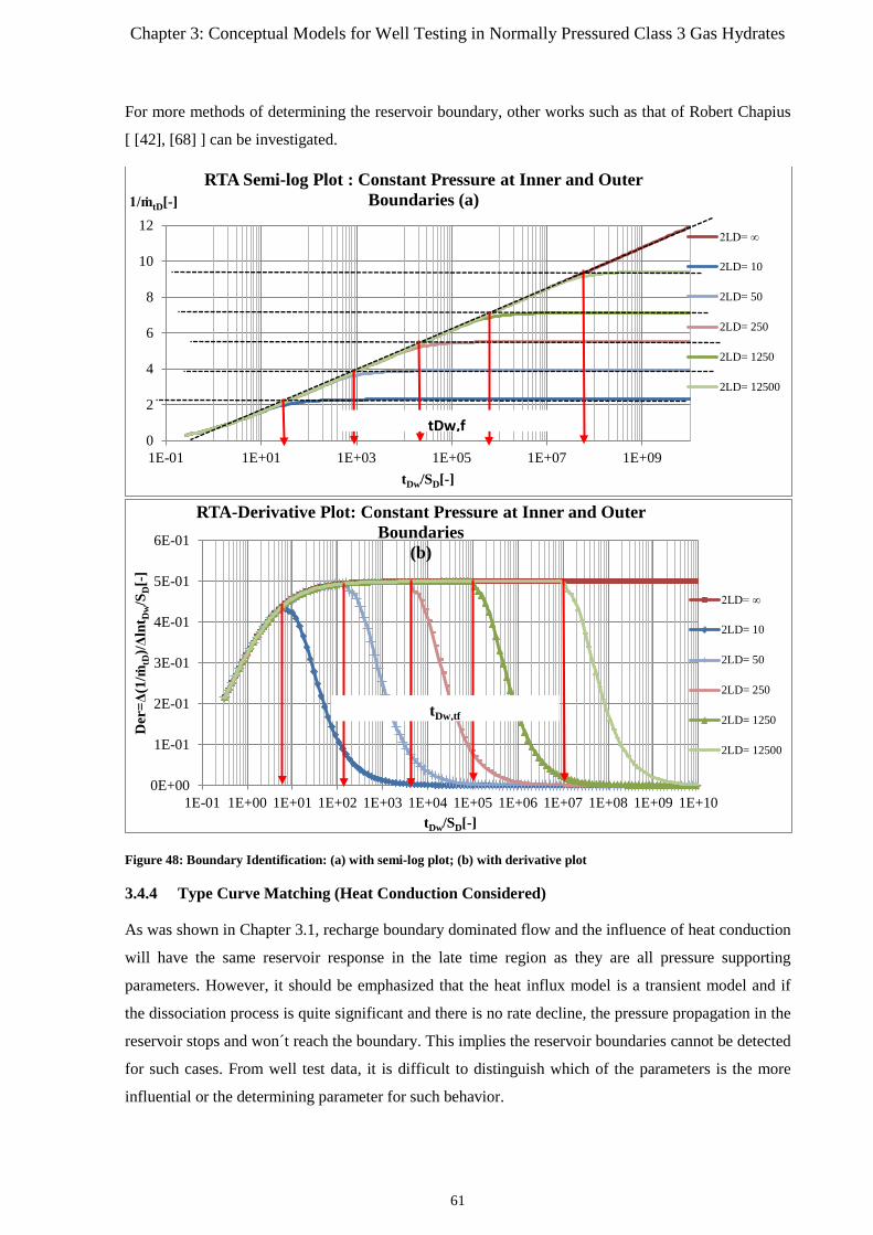
Chapter 3: Conceptual Models for Well Testing in Normally Pressured Class 3 Gas Hydrates
For more methods of determining the reservoir boundary, other works such as that of Robert Chapius
[ [42], [68] ] can be investigated.
Figure 48: Boundary Identification: (a) with semi-log plot; (b) with derivative plot
3.4.4 Type Curve Matching (Heat Conduction Considered)
As was shown in Chapter 3.1, recharge boundary dominated flow and the influence of heat conduction
will have the same reservoir response in the late time region as they are all pressure supporting
parameters. However, it should be emphasized that the heat influx model is a transient model and if
the dissociation process is quite significant and there is no rate decline, the pressure propagation in the
reservoir stops and won´t reach the boundary. This implies the reservoir boundaries cannot be detected
for such cases. From well test data, it is difficult to distinguish which of the parameters is the more
influential or the determining parameter for such behavior.
0
2
4
6
8
10
12
1E-01 1E+01 1E+03 1E+05 1E+07 1E+09
1/ṁtD[-]
tDw/SD[-]
RTA Semi-log Plot : Constant Pressure at Inner and Outer Boundaries (a)
2LD= ∞
2LD= 10
2LD= 50
2LD= 250
2LD= 1250
2LD= 12500
tDw,f
0E+00
1E-01
2E-01
3E-01
4E-01
5E-01
6E-01
1E-01 1E+00 1E+01 1E+02 1E+03 1E+04 1E+05 1E+06 1E+07 1E+08 1E+09 1E+10
Der
=Δ(1
/ṁtD
)/Δln
t Dw/S
D[-
]
tDw/SD[-]
RTA-Derivative Plot: Constant Pressure at Inner and Outer Boundaries
(b)
2LD= ∞
2LD= 10
2LD= 50
2LD= 250
2LD= 1250
2LD= 12500
tDw,tf
61
Chapter 3: Conceptual Models for Well Testing in Normally Pressured Class 3 Gas Hydrates
For reservoirs with impermeable boundaries (NFB) the no flow boundary behavior might occur before
the influence of heat conduction has a significant pressure support behavior on the reservoir response
as seen in Figure 39. In such cases, it is possible to derive both the distance to boundary and make an
estimate of the heat influx terms.
For the type curve matching method addressed here, we will ignore the effects of boundary and
propose the type curve match required to estimate the reservoir parameters during transient flow
regimes.
The type curve has an advantage over the semi-log plot in that the reservoir parameters are estimated
at each time step whereas we obtain average values using the semi-log plot. As seen with the semi-log
plots, the reciprocal of the rate transient is a much better method of characterizing the reservoir from a
log scale. Hence, the type-curve matching done on a semi-log scale should be performed using the
reciprocal of the rate transient.
Required Plots
• 1mtD
Versus tDw
• 1mt
Versus t
• φPI(t) Versus t
Time Match
The time match points along the vertical are:
� tDwSDµD
�MP
; tMP; ��bD�MP 3. 77
Where,
tDw = tk∅rw2
ft(pi)β(pi)
From the match points, the dimensionless interlayer heat flux compressibility is derived thus:
[SDµD]MP = tDw� tDwSDµD
�MP
= k∅rw2
ft(pi)β(pi)
tMP
� tDwSDµD�MP
3. 78
Rate Match
The match along the horizontal is given by:
�1
mtD�MP
; �1
mt�MP
; [φPI(t)]g,MP
62
Chapter 3: Conceptual Models for Well Testing in Normally Pressured Class 3 Gas Hydrates
From the match points, the effective permeabilities of the different phases are derived thus:
[k∫ ft(p)dp]𝑀𝑀𝑀𝑀 =� 1mtD
�MP
2πh� 1mt�MP
3. 79
Conventionally, the match point of the multiphase pseudo-pressure at the wellbore would be a
constant value from the imposed inner boundary condition used in deriving the models for this work.
If this is not the case, the use of the type curve matching techniques will depict changing values and
can still be used to derive the effective permeability of the flowing phases.
kkrg∗ (p) = [φPI(t)]g,MP �1mt�MP
[k∫ ft(p)dp]𝑀𝑀𝑀𝑀 3. 80
Where,
[φPI(t)]𝑔𝑔 =Qg,stρg,st
∫ρgɳg
dp=
Qg,st
∫ 1Bgɳg
dp
Water Phase
Similarly, the effective permeability of the water phase could be given thus:
kkrw∗ (p) = [φPI(t)]wmt
[k∫ ft(p)dp] 3. 81
For mass conservation to be valid and to improve on the accuracy of the match points, the following
mass conservation equation must be valid:
mg(t)+mw(t)
mt=
2πh���kkrg∗ (p)�MP�∫
1Bgɳg
dppipwf
��+��kkrw∗ (p)�MP�∫
1Bwɳw
dppipwf
���[mtD]MP
mt= 1 3. 82
3.5 Pressure Transient Analysis in Normally Pressured Gas Hydrate
Reservoirs
As mentioned earlier, pressure transient analysis in normally pressured gas hydrates could be handled
likewise conventional gas reservoirs, however considering multiphase aspects. It is still worth
mentioning that the assumptions of constant sandface rate or even surface rates are hardly achieved
during well test analysis, especially with multiphase systems.
As was seen with the rate transient solution, the models have to be represented such that the measured
data during the test (here the pressure) can be analyzed. With RTA, the linearized models were
represented in terms of the transient total mass rate which is measurable from well test data, whereas
in PTA the linearized models were represented in terms of the transient total pseudo-pressure which is
not directly measured. This implies for a proper analysis of the pressure transient data, the
computation of the pseudo-pressure of the reservoir system should be performed, which is
63
Chapter 3: Conceptual Models for Well Testing in Normally Pressured Class 3 Gas Hydrates
unfortunately not possible for newly tested reservoirs. As a result, the models will further be
simplified such that effective permeabilities of the different phases can be estimated.
Multiphase
φD = 2πhk∫ρt�
krɳ �t
dp
mt= 2πhk ∫ ft(p)dp
mt 3. 83
Gas Phase
Qg,st = 1φD
[2πhk∫ ft(p)dp]ρg,st
fm,g 3. 84
Qg,st = 1φD
�2πhk∫ fg(p)dp�ρg,st
3. 85
Water Phase
Qw,st = 1φD
[2πhk∫ ft(p)dp]ρw,st
fm,w 3. 86
Qw,st = 1φD
[2πhk∫ fw(p)dp]ρw,st
3. 87
Due to the constantly changing flow rate of the different phases during the pressure transient test for
the multiphase system, the pseudo-pressure normalized rate method is best used to analyze the data as
will be shown later.
Pressure Transient Analysis (PTA)
Depending on the rate of change of relative permeability of the fluid in question, the flow rate could
be very time dependent, which makes the analysis of pressure transient responses difficult. For this
reason, the pseudo reciprocal productivity index (rate normalized pseudo-pressure) is once more a
good tool for analysis. However, Convolution/Deconvolution techniques could be most suitable for
analysis of such reservoir responses.
∫ρgɳg
dp
Qg,st(t)ρg,st=∫ 1
Bgɳgdp
Qg,st(t) = �φRPI(t)�𝑔𝑔 =1
2πhkkrg∗ (p)φD
The rate normalized pseudo-pressure (pseudo reciprocal productivity index) representation above
gives a relationship between the transient flow rate and the pseudo-pressure which is transient in this
case for constant total sandface rate tests.
The PTA MBM during IARF is simplified for semi-log analysis thus:
Range: 10²<tDw/μDSD<104 and �eD
(∆zD−1) < 0.01
[φRPI(t)]𝑔𝑔 = 1.15152πhkkrg∗ (p) �logt + log � k
∅rw2ft(pi)β(pi)
� − log(µDSD) + 0.3513� 3. 88
64

Chapter 3: Conceptual Models for Well Testing in Normally Pressured Class 3 Gas Hydrates
The same methods applied for RTA are applicable here with the above representation of the gas rate
normalized pseudo-pressure. The characteristics of the rate normalized pseudo-pressure in this case are
as follows:
• The pressure transient in the rate normalized pseudo-pressure reflects the reservoir behavior
and hydrate dissociation effects
• The rate transient in the model reflects the changes in the effective permeability of the phase
in question. Hence if the flow rate of a phase remains constant during production, a semi-log
plot of the analysis could be made for the IARF model given above. However, for changing
flow rates, the use of semi-log plots becomes impracticable; nonetheless, the semi-log analysis
will still be addressed.
3.5.1 Semi-log Analysis
[φRPI(t)]g Versus t
The gradient of the semi-log plot:
mlog = 1.15152πhkkrg∗ (p) 3. 89
Effective gas permeability at IARF
kkrg∗ (p) = kg∗(p) = 1.15152πhmlog
3. 90
Dimensionless Dissociation Terms (IARF)
Applying the damage skin approach for well test analysis we get an approximation of the dissociation
terms for the hydrate layer.
(SDµD)avg = �SD + FCDeD(∆zD−1)3
�avg
≈ exp �−0.434 ��[φRPI(t)]g�t=1s
mlog− log � k
∅rw2ft(pi)β(pi)
∗ 100.3513��� 3. 91
3.5.2 Pressure Derivative Analysis
Analogue derivative plots seen in RTA, the rate normalized pseudo-pressure can be applied for
pressure transient analysis.
d�[φRPI(t)]𝑔𝑔�dlnt
=0.5
2πhkkrg∗ (p) = Der
log �d[φRPI(t)]𝑔𝑔
dtt� vs logt 3. 92
If the derivative is time independent, the log-log plot will remain constant during IARF. The apparent
effective gas permeability is given by (see Appendix 10 for details):
kg,avg∗ (p) = 0.5
2πhDer 3. 93
65

Chapter 3: Conceptual Models for Well Testing in Normally Pressured Class 3 Gas Hydrates
3.5.3 Type Curve Matching (Heat Conduction Considered)
Required Plots
• φD Versus tDw
• [φi − φwf(t)] Versus t
• φRPI(t) Versus t
Time Match
The time match points along the vertical are:
� tDwSDµD
�MP
; tMP; ��bD�MP 3. 94
Where,
tDw = tk∅rw2
ft(pi)β(pi)
From the match points, the dimensionless interlayer heat flux compressibility is derived thus:
[SDµD]MP = tDw� tDwSDµD
�MP
= k∅rw2
ft(pi)β(pi)
tMP
� tDwSDµD�MP
3. 95
Pressure Match
The match along the horizontal is given by:
[φD]MP ; [φRPI(t)]g,MP; [φi − φwf]MP
To perform the pressure matches above requires the use of the pseudo-pressure of the total system
which is usually an unknown parameter for a newly tested reservoir and cannot be derived directly
from the well test data as in the case of RTA. Hence, the pressure matching techniques to derive the
effective permeability for different time could be very cumbersome.
66
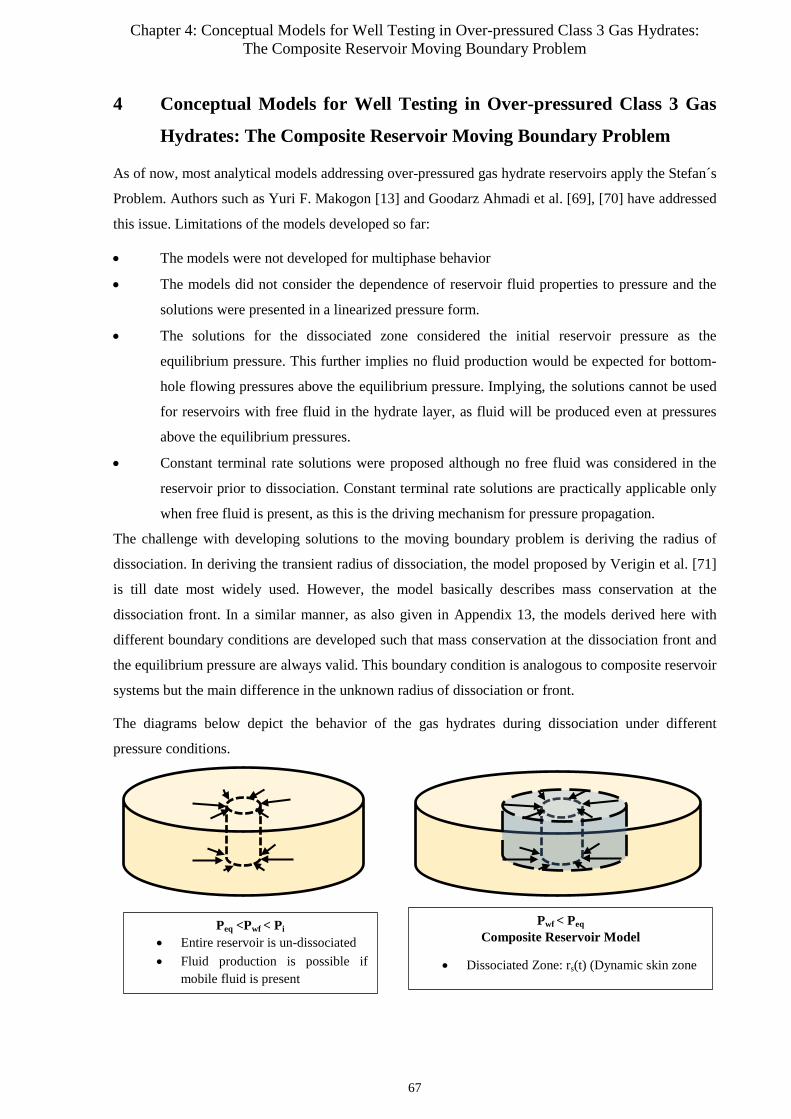
Chapter 4: Conceptual Models for Well Testing in Over-pressured Class 3 Gas Hydrates: The Composite Reservoir Moving Boundary Problem
4 Conceptual Models for Well Testing in Over-pressured Class 3 Gas
Hydrates: The Composite Reservoir Moving Boundary Problem
As of now, most analytical models addressing over-pressured gas hydrate reservoirs apply the Stefan´s
Problem. Authors such as Yuri F. Makogon [13] and Goodarz Ahmadi et al. [69], [70] have addressed
this issue. Limitations of the models developed so far:
• The models were not developed for multiphase behavior
• The models did not consider the dependence of reservoir fluid properties to pressure and the
solutions were presented in a linearized pressure form.
• The solutions for the dissociated zone considered the initial reservoir pressure as the
equilibrium pressure. This further implies no fluid production would be expected for bottom-
hole flowing pressures above the equilibrium pressure. Implying, the solutions cannot be used
for reservoirs with free fluid in the hydrate layer, as fluid will be produced even at pressures
above the equilibrium pressures.
• Constant terminal rate solutions were proposed although no free fluid was considered in the
reservoir prior to dissociation. Constant terminal rate solutions are practically applicable only
when free fluid is present, as this is the driving mechanism for pressure propagation.
The challenge with developing solutions to the moving boundary problem is deriving the radius of
dissociation. In deriving the transient radius of dissociation, the model proposed by Verigin et al. [71]
is till date most widely used. However, the model basically describes mass conservation at the
dissociation front. In a similar manner, as also given in Appendix 13, the models derived here with
different boundary conditions are developed such that mass conservation at the dissociation front and
the equilibrium pressure are always valid. This boundary condition is analogous to composite reservoir
systems but the main difference in the unknown radius of dissociation or front.
The diagrams below depict the behavior of the gas hydrates during dissociation under different
pressure conditions.
Peq <Pwf < Pi • Entire reservoir is un-dissociated • Fluid production is possible if
mobile fluid is present
Pwf < Peq Composite Reservoir Model
• Dissociated Zone: rs(t) (Dynamic skin zone
67
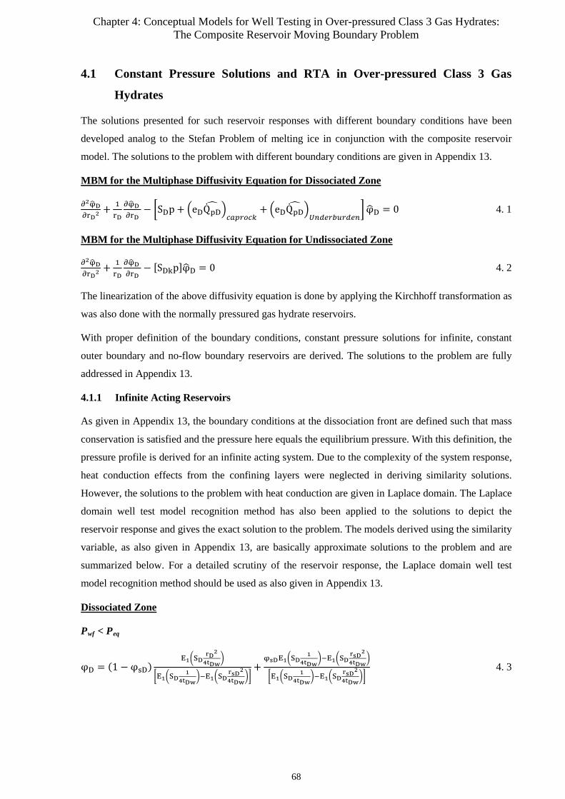
Chapter 4: Conceptual Models for Well Testing in Over-pressured Class 3 Gas Hydrates: The Composite Reservoir Moving Boundary Problem
4.1 Constant Pressure Solutions and RTA in Over-pressured Class 3 Gas
Hydrates
The solutions presented for such reservoir responses with different boundary conditions have been
developed analog to the Stefan Problem of melting ice in conjunction with the composite reservoir
model. The solutions to the problem with different boundary conditions are given in Appendix 13.
MBM for the Multiphase Diffusivity Equation for Dissociated Zone
∂2φ�D∂rD2
+ 1rD
∂φ�D ∂rD
− �SDp + �eDQpD� �
𝐶𝐶𝐶𝐶𝐶𝐶𝐶𝐶𝐶𝐶𝐶𝐶𝑘𝑘+ �eDQpD
� �𝑈𝑈𝑈𝑈𝑈𝑈𝑈𝑈𝐶𝐶𝑈𝑈𝑈𝑈𝐶𝐶𝑈𝑈𝑈𝑈𝑈𝑈
�φ�D = 0 4. 1
MBM for the Multiphase Diffusivity Equation for Undissociated Zone
∂2φ�D∂rD2
+ 1rD
∂φ�D ∂rD
− [SDkp]φ�D = 0 4. 2
The linearization of the above diffusivity equation is done by applying the Kirchhoff transformation as
was also done with the normally pressured gas hydrate reservoirs.
With proper definition of the boundary conditions, constant pressure solutions for infinite, constant
outer boundary and no-flow boundary reservoirs are derived. The solutions to the problem are fully
addressed in Appendix 13.
4.1.1 Infinite Acting Reservoirs
As given in Appendix 13, the boundary conditions at the dissociation front are defined such that mass
conservation is satisfied and the pressure here equals the equilibrium pressure. With this definition, the
pressure profile is derived for an infinite acting system. Due to the complexity of the system response,
heat conduction effects from the confining layers were neglected in deriving similarity solutions.
However, the solutions to the problem with heat conduction are given in Laplace domain. The Laplace
domain well test model recognition method has also been applied to the solutions to depict the
reservoir response and gives the exact solution to the problem. The models derived using the similarity
variable, as also given in Appendix 13, are basically approximate solutions to the problem and are
summarized below. For a detailed scrutiny of the reservoir response, the Laplace domain well test
model recognition method should be used as also given in Appendix 13.
Dissociated Zone
Pwf < Peq
φD = (1 − φsD)E1�SD
rD2
4tDw�
�E1�SD1
4tDw�−E1�SD
rsD2
4tDw��
+φsDE1�SD
14tDw
�−E1�SDrsD
2
4tDw�
�E1�SD1
4tDw�−E1�SD
rsD2
4tDw��
4. 3
68
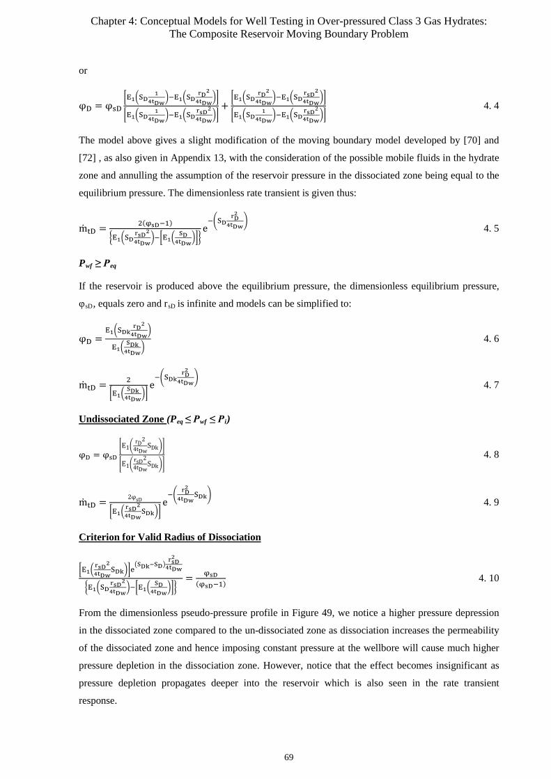
Chapter 4: Conceptual Models for Well Testing in Over-pressured Class 3 Gas Hydrates: The Composite Reservoir Moving Boundary Problem
or
φD = φsD�E1�SD
14tDw
�−E1�SDrD2
4tDw��
�E1�SD1
4tDw�−E1�SD
rsD2
4tDw��
+�E1�SD
rD2
4tDw�−E1�SD
rsD2
4tDw��
�E1�SD1
4tDw�−E1�SD
rsD2
4tDw��
4. 4
The model above gives a slight modification of the moving boundary model developed by [70] and
[72] , as also given in Appendix 13, with the consideration of the possible mobile fluids in the hydrate
zone and annulling the assumption of the reservoir pressure in the dissociated zone being equal to the
equilibrium pressure. The dimensionless rate transient is given thus:
mtD = 2(φsD−1)
�E1�SDrsD2
4tDw�−�E1�
SD4tDw
���e−�SD
rD2
4tDw� 4. 5
Pwf ≥ Peq
If the reservoir is produced above the equilibrium pressure, the dimensionless equilibrium pressure,
φsD, equals zero and rsD is infinite and models can be simplified to:
φD =E1�SDk
rD2
4tDw�
E1�SDk4tDw
� 4. 6
mtD = 2
�E1�SDk4tDw
��e−�SDk
rD2
4tDw� 4. 7
Undissociated Zone (Peq ≤ Pwf ≤ Pi)
φD = φsD
�E1�rD2
4tDwSDk��
�E1�rsD24tDw
SDk�� 4. 8
mtD = 2φsD
�E1�rsD2
4tDwSDk��
e−�
rD2
4tDwSDk�
4. 9
Criterion for Valid Radius of Dissociation
�E1�rsD
2
4tDwSDk��e
�SDk−SD�rsD2
4tDw
�E1�SDrsD2
4tDw�−�E1�
SD4tDw
���= φsD
(φsD−1) 4. 10
From the dimensionless pseudo-pressure profile in Figure 49, we notice a higher pressure depression
in the dissociated zone compared to the un-dissociated zone as dissociation increases the permeability
of the dissociated zone and hence imposing constant pressure at the wellbore will cause much higher
pressure depletion in the dissociation zone. However, notice that the effect becomes insignificant as
pressure depletion propagates deeper into the reservoir which is also seen in the rate transient
response.
69
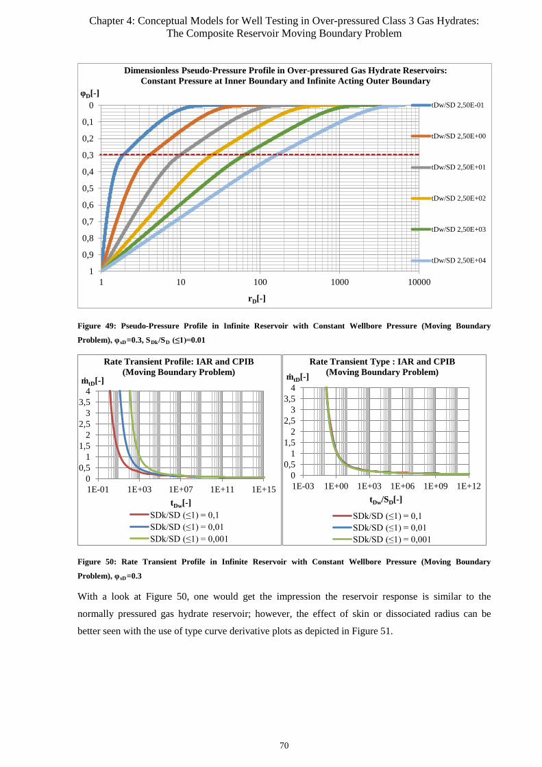
Chapter 4: Conceptual Models for Well Testing in Over-pressured Class 3 Gas Hydrates: The Composite Reservoir Moving Boundary Problem
Figure 49: Pseudo-Pressure Profile in Infinite Reservoir with Constant Wellbore Pressure (Moving Boundary
Problem), φsD=0.3, SDk/SD (≤1)=0.01
Figure 50: Rate Transient Profile in Infinite Reservoir with Constant Wellbore Pressure (Moving Boundary
Problem), φsD=0.3
With a look at Figure 50, one would get the impression the reservoir response is similar to the
normally pressured gas hydrate reservoir; however, the effect of skin or dissociated radius can be
better seen with the use of type curve derivative plots as depicted in Figure 51.
0
0,1
0,2
0,3
0,4
0,5
0,6
0,7
0,8
0,9
11 10 100 1000 10000
φD[-]
rD[-]
Dimensionless Pseudo-Pressure Profile in Over-pressured Gas Hydrate Reservoirs: Constant Pressure at Inner Boundary and Infinite Acting Outer Boundary
tDw/SD 2,50E-01
tDw/SD 2,50E+00
tDw/SD 2,50E+01
tDw/SD 2,50E+02
tDw/SD 2,50E+03
tDw/SD 2,50E+04
00,5
11,5
22,5
33,5
4
1E-01 1E+03 1E+07 1E+11 1E+15
ṁtD[-]
tDw[-]
Rate Transient Profile: IAR and CPIB (Moving Boundary Problem)
SDk/SD (≤1) = 0,1 SDk/SD (≤1) = 0,01 SDk/SD (≤1) = 0,001
00,5
11,5
22,5
33,5
4
1E-03 1E+00 1E+03 1E+06 1E+09 1E+12
ṁtD[-]
tDw/SD[-]
Rate Transient Type : IAR and CPIB (Moving Boundary Problem)
SDk/SD (≤1) = 0,1 SDk/SD (≤1) = 0,01 SDk/SD (≤1) = 0,001
70
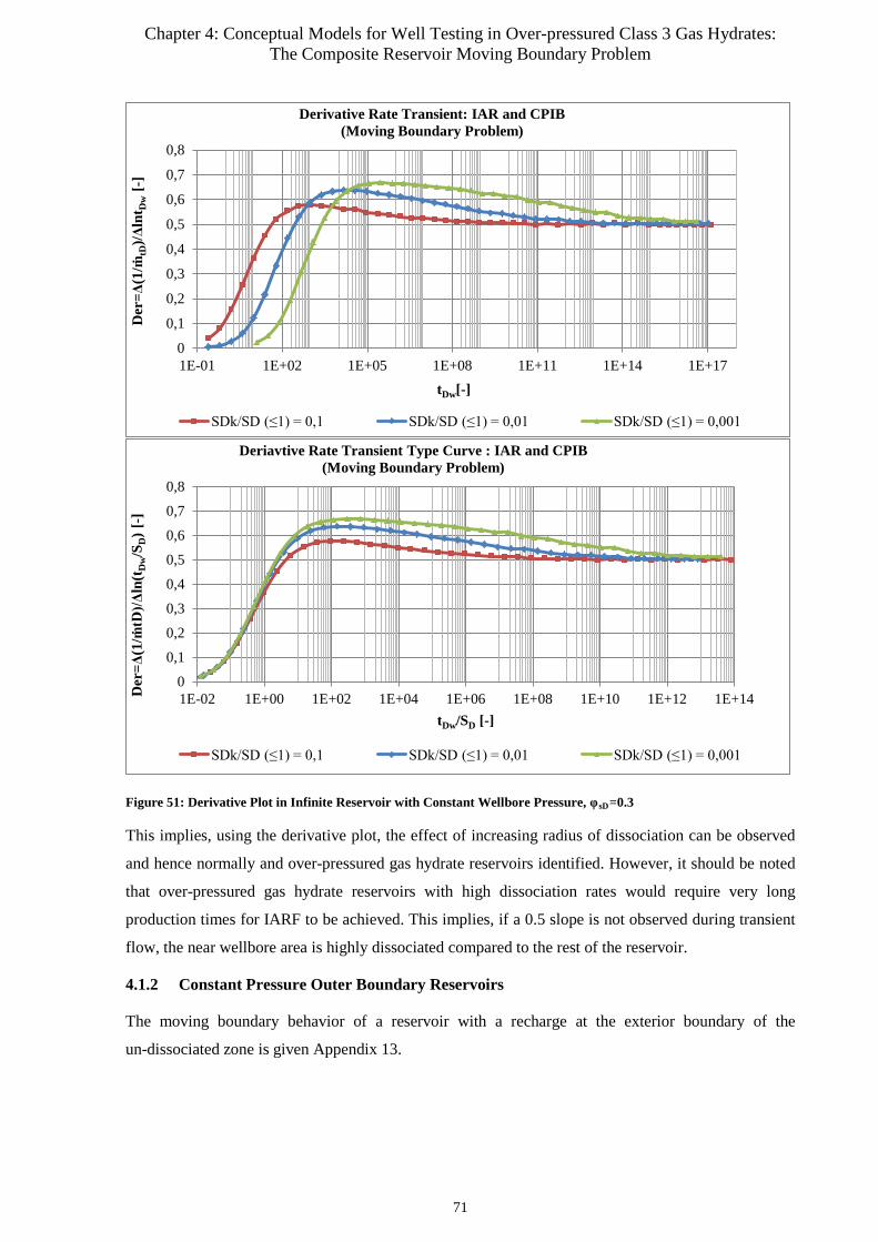
Chapter 4: Conceptual Models for Well Testing in Over-pressured Class 3 Gas Hydrates: The Composite Reservoir Moving Boundary Problem
Figure 51: Derivative Plot in Infinite Reservoir with Constant Wellbore Pressure, φsD=0.3
This implies, using the derivative plot, the effect of increasing radius of dissociation can be observed
and hence normally and over-pressured gas hydrate reservoirs identified. However, it should be noted
that over-pressured gas hydrate reservoirs with high dissociation rates would require very long
production times for IARF to be achieved. This implies, if a 0.5 slope is not observed during transient
flow, the near wellbore area is highly dissociated compared to the rest of the reservoir.
4.1.2 Constant Pressure Outer Boundary Reservoirs
The moving boundary behavior of a reservoir with a recharge at the exterior boundary of the
un-dissociated zone is given Appendix 13.
0
0,1
0,2
0,3
0,4
0,5
0,6
0,7
0,8
1E-01 1E+02 1E+05 1E+08 1E+11 1E+14 1E+17
Der
=Δ(1
/ṁtD
)/Δln
t Dw [-
]
tDw[-]
Derivative Rate Transient: IAR and CPIB (Moving Boundary Problem)
SDk/SD (≤1) = 0,1 SDk/SD (≤1) = 0,01 SDk/SD (≤1) = 0,001
0
0,1
0,2
0,3
0,4
0,5
0,6
0,7
0,8
1E-02 1E+00 1E+02 1E+04 1E+06 1E+08 1E+10 1E+12 1E+14Der
=Δ(1
/ṁtD
)/Δln
(tD
w/S
D) [
-]
tDw/SD [-]
Deriavtive Rate Transient Type Curve : IAR and CPIB (Moving Boundary Problem)
SDk/SD (≤1) = 0,1 SDk/SD (≤1) = 0,01 SDk/SD (≤1) = 0,001
71

Chapter 4: Conceptual Models for Well Testing in Over-pressured Class 3 Gas Hydrates: The Composite Reservoir Moving Boundary Problem
The models could be summarized below:
Dissociated Zone
Pwf < Peq
φD = φsD�E1�SD
14tDw
�−E1�SDrD2
4tDw��
�E1�SD1
4tDw�−E1�SD
rsD2
4tDw��
+�E1�SD
rD2
4tDw�−E1�SD
rsD2
4tDw��
�E1�SD1
4tDw�−E1�SD
rsD2
4tDw��
4. 11
mtD = 2�φsD−1�
�E1�SDrsD2
4tDw�−�E1�SD
14tDw
���e−�SD
rD2
4tDw� 4. 12
Pwf ≥ Peq
φD =�E1�
rD2
4tDwSDk��−�E1�
�2lD−rD�2
4tDwSDk��
�E1�1
4tDwSDk��−�E1�
�2lD−1�2
4tDwSDk��
4. 13
mtD = 2
�E1�SDk4tDw
��−�E1��2lD−1�
2
4tDwSDk��
�e−� rD2
4tDwSDk� + (2lD − rD)−1rDe−
�2lD−rD�2
4tDwSDk� 4. 14
Undissociated Zone
φD = φsD�E1�
rD2
4tDwSDk��−�E1�
�2lD−rD�2
4tDwSDk��
�E1�rsD2
4tDwSDk��−�E1�
�2lD−rsD�2
4tDwSDk��
4. 15
mtD = 2φsD
�E1�rsD2
4tDwSDk��−�E1�
�2lD−rsD�2
4tDwSDk��
�e−� rD2
4tDwSDk� + (2lD − rD)−1rDe−
�2lD−rD�2
4tDwSDk� 4. 16
Criterion for Valid Radius of Dissociation (Pavg ≥ Peq)
e−SD
rsD2
4tDw
�e−�
rsD24tDw
SDk�+(2lD−rsD)−1rsDe−�2lD−rsD�
2
4tDwSDk�
�E1�rsD
2
4tDwSDk�−E1�
�2lD−rsD�2
4tDwSDk��
�E1�rsD2
4tDwSD�−�E1�
SD4tDw
���= φsD
(φsD−1) 4. 17
72
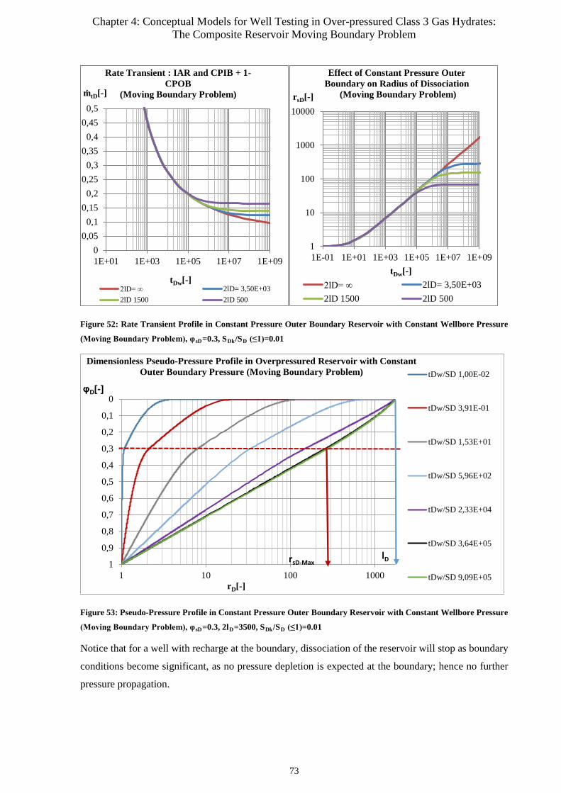
Chapter 4: Conceptual Models for Well Testing in Over-pressured Class 3 Gas Hydrates: The Composite Reservoir Moving Boundary Problem
Figure 52: Rate Transient Profile in Constant Pressure Outer Boundary Reservoir with Constant Wellbore Pressure
(Moving Boundary Problem), φsD=0.3, SDk/SD (≤1)=0.01
Figure 53: Pseudo-Pressure Profile in Constant Pressure Outer Boundary Reservoir with Constant Wellbore Pressure
(Moving Boundary Problem), φsD=0.3, 2lD=3500, SDk/SD (≤1)=0.01
Notice that for a well with recharge at the boundary, dissociation of the reservoir will stop as boundary
conditions become significant, as no pressure depletion is expected at the boundary; hence no further
pressure propagation.
00,05
0,10,15
0,20,25
0,30,35
0,40,45
0,5
1E+01 1E+03 1E+05 1E+07 1E+09
ṁtD[-]
tDw[-]
Rate Transient : IAR and CPIB + 1-CPOB
(Moving Boundary Problem)
2lD= ∞ 2lD= 3,50E+032lD 1500 2lD 500
1
10
100
1000
10000
1E-01 1E+01 1E+03 1E+05 1E+07 1E+09
rsD[-]
tDw[-]
Effect of Constant Pressure Outer Boundary on Radius of Dissociation
(Moving Boundary Problem)
2lD= ∞ 2lD= 3,50E+032lD 1500 2lD 500
0
0,1
0,2
0,3
0,4
0,5
0,6
0,7
0,8
0,9
11 10 100 1000
φD[-]
rD[-]
Dimensionless Pseudo-Pressure Profile in Overpressured Reservoir with Constant Outer Boundary Pressure (Moving Boundary Problem) tDw/SD 1,00E-02
tDw/SD 3,91E-01
tDw/SD 1,53E+01
tDw/SD 5,96E+02
tDw/SD 2,33E+04
tDw/SD 3,64E+05
tDw/SD 9,09E+05
rsD-Max lD
73
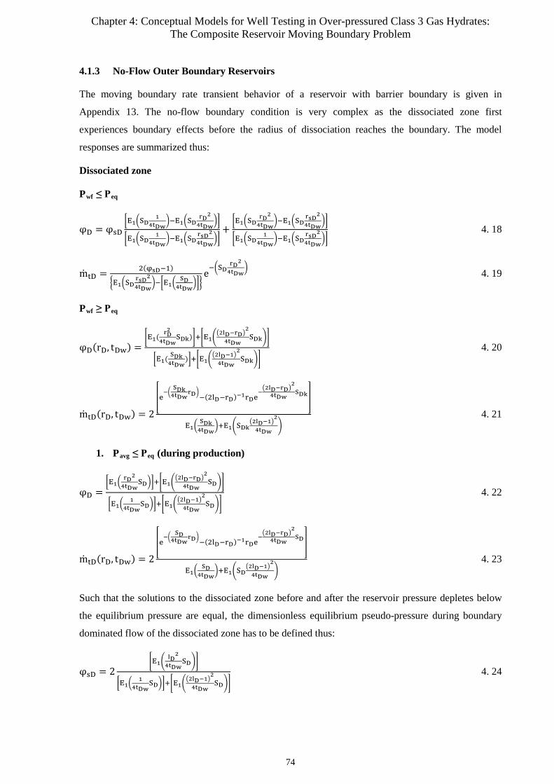
Chapter 4: Conceptual Models for Well Testing in Over-pressured Class 3 Gas Hydrates: The Composite Reservoir Moving Boundary Problem
4.1.3 No-Flow Outer Boundary Reservoirs
The moving boundary rate transient behavior of a reservoir with barrier boundary is given in
Appendix 13. The no-flow boundary condition is very complex as the dissociated zone first
experiences boundary effects before the radius of dissociation reaches the boundary. The model
responses are summarized thus:
Dissociated zone
Pwf ≤ Peq
φD = φsD�E1�SD
14tDw
�−E1�SDrD2
4tDw��
�E1�SD1
4tDw�−E1�SD
rsD2
4tDw��
+�E1�SD
rD2
4tDw�−E1�SD
rsD2
4tDw��
�E1�SD1
4tDw�−E1�SD
rsD2
4tDw��
4. 18
mtD = 2(φsD−1)
�E1�SDrsD2
4tDw�−�E1�
SD4tDw
���e−�SD
rD2
4tDw� 4. 19
Pwf ≥ Peq
φD(rD, tDw) =�E1(
rD2
4tDwSDk)�+�E1�
�2lD−rD�2
4tDwSDk��
�E1( SDk4tDw
)�+�E1��2lD−1�
2
4tDwSDk��
4. 20
mtD(rD, tDw) = 2
�e−�
SDk4tDw
rD�−(2lD−rD)−1rDe−�2lD−rD�
2
4tDwSDk�
E1�SDk4tDw
�+E1�SDk�2lD−1�
2
4tDw�
4. 21
1. Pavg ≤ Peq (during production)
φD =�E1�
rD2
4tDwSD��+�E1�
�2lD−rD�2
4tDwSD��
�E1�1
4tDwSD��+�E1�
�2lD−1�2
4tDwSD��
4. 22
mtD(rD, tDw) = 2
�e−�
SD4tDw
rD�−(2lD−rD)−1rDe−�2lD−rD�
2
4tDwSD�
E1�SD
4tDw�+E1�SD
�2lD−1�2
4tDw�
4. 23
Such that the solutions to the dissociated zone before and after the reservoir pressure depletes below
the equilibrium pressure are equal, the dimensionless equilibrium pseudo-pressure during boundary
dominated flow of the dissociated zone has to be defined thus:
φsD = 2�E1�
lD2
4tDwSD��
�E1�1
4tDwSD��+�E1�
�2lD−1�2
4tDwSD��
4. 24
74
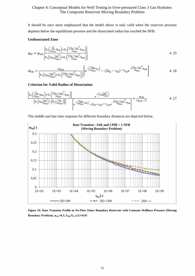
Chapter 4: Conceptual Models for Well Testing in Over-pressured Class 3 Gas Hydrates: The Composite Reservoir Moving Boundary Problem
It should be once more emphasized that the model above is only valid when the reservoir pressure
depletes below the equilibrium pressure and the dissociated radius has reached the NFB.
Undissociated Zone
φD = φsD�E1�
rD2
4tDwSDk�+E1�
�2lD−rD�2
4tDwSDk��
�E1�SDkrsD2
4tDw�+E1�
�2lD−rsD�2
4tDwSDk��
4. 25
mtD = 2φsD
�E1�SDkrsD2
4tDw�+E1�
�2lD−rsD�2
4tDwSDk��
�e−� SDk
4tDwrD� − (2lD − rD)−1rDe−
�2lD−rD�2
4tDwSDk� 4. 26
Criterion for Valid Radius of Dissociation
�E1�rsD2
4tDwSDk�+E1�
�2lD−rsD�2
4tDwSDk��
�E1�SDrsD2
4tDw�−�E1�
SD4tDw
���
e−�SD
rsD24tDw
�
�e−�
SDk4tDw
rsD�−(2lD−rsD)−1rsDe−�2lD−rsD�
2
4tDwSDk�
= φsD(φsD−1) 4. 27
The middle and late time response for different boundary distances are depicted below.
Figure 54: Rate Transient Profile in No-Flow Outer Boundary Reservoir with Constant Wellbore Pressure (Moving
Boundary Problem), φsD=0.3, SDk/SD (≤1)=0.01
0
0,05
0,1
0,15
0,2
0,25
0,3
1E+02 1E+03 1E+04 1E+05 1E+06 1E+07 1E+08 1E+09
ṁtD[-]
tDw[-]
Rate Transient : IAR and CPIB + 1-NFB (Moving Boundary Problem)
2lD 500 2lD 1500 2lD= ∞
75
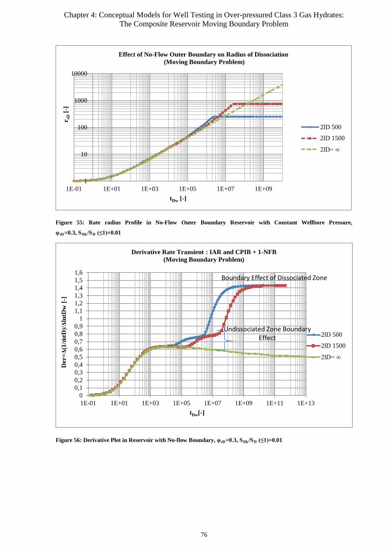
Chapter 4: Conceptual Models for Well Testing in Over-pressured Class 3 Gas Hydrates: The Composite Reservoir Moving Boundary Problem
Figure 55: Rate radius Profile in No-Flow Outer Boundary Reservoir with Constant Wellbore Pressure,
φsD=0.3, SDk/SD (≤1)=0.01
Figure 56: Derivative Plot in Reservoir with No-flow Boundary, φsD=0.3, SDk/SD (≤1)=0.01
1
10
100
1000
10000
1E-01 1E+01 1E+03 1E+05 1E+07 1E+09
r sD [-
]
tDw [-]
Effect of No-Flow Outer Boundary on Radius of Dissociation (Moving Boundary Problem)
2lD 500
2lD 1500
2lD= ∞
00,10,20,30,40,50,60,70,80,9
11,11,21,31,41,51,6
1E-01 1E+01 1E+03 1E+05 1E+07 1E+09 1E+11 1E+13
Der
=Δ(1
/ṁtD
)/Δln
tDw
[-]
tDw[-]
Derivative Rate Transient : IAR and CPIB + 1-NFB (Moving Boundary Problem)
2lD 500
2lD 1500
2lD= ∞
Undissociated Zone Boundary Effect
Boundary Effect of Dissociated Zone
76
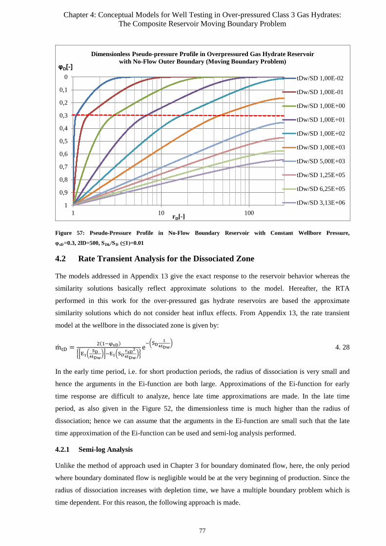
Chapter 4: Conceptual Models for Well Testing in Over-pressured Class 3 Gas Hydrates: The Composite Reservoir Moving Boundary Problem
Figure 57: Pseudo-Pressure Profile in No-Flow Boundary Reservoir with Constant Wellbore Pressure,
φsD=0.3, 2lD=500, SDk/SD (≤1)=0.01
4.2 Rate Transient Analysis for the Dissociated Zone
The models addressed in Appendix 13 give the exact response to the reservoir behavior whereas the
similarity solutions basically reflect approximate solutions to the model. Hereafter, the RTA
performed in this work for the over-pressured gas hydrate reservoirs are based the approximate
similarity solutions which do not consider heat influx effects. From Appendix 13, the rate transient
model at the wellbore in the dissociated zone is given by:
mtD = 2(1−φsD)
��E1�SD
4tDw��−E1�SD
rsD2
4tDw��
e−�SD1
4tDw� 4. 28
In the early time period, i.e. for short production periods, the radius of dissociation is very small and
hence the arguments in the Ei-function are both large. Approximations of the Ei-function for early
time response are difficult to analyze, hence late time approximations are made. In the late time
period, as also given in the Figure 52, the dimensionless time is much higher than the radius of
dissociation; hence we can assume that the arguments in the Ei-function are small such that the late
time approximation of the Ei-function can be used and semi-log analysis performed.
4.2.1 Semi-log Analysis
Unlike the method of approach used in Chapter 3 for boundary dominated flow, here, the only period
where boundary dominated flow is negligible would be at the very beginning of production. Since the
radius of dissociation increases with depletion time, we have a multiple boundary problem which is
time dependent. For this reason, the following approach is made.
0
0,1
0,2
0,3
0,4
0,5
0,6
0,7
0,8
0,9
11 10 100
φD[-]
rD[-]
Dimensionless Pseudo-pressure Profile in Overpressured Gas Hydrate Reservoir with No-Flow Outer Boundary (Moving Boundary Problem)
tDw/SD 1,00E-02
tDw/SD 1,00E-01
tDw/SD 1,00E+00
tDw/SD 1,00E+01
tDw/SD 1,00E+02
tDw/SD 1,00E+03
tDw/SD 5,00E+03
tDw/SD 1,25E+05
tDw/SD 6,25E+05
tDw/SD 3,13E+06
77
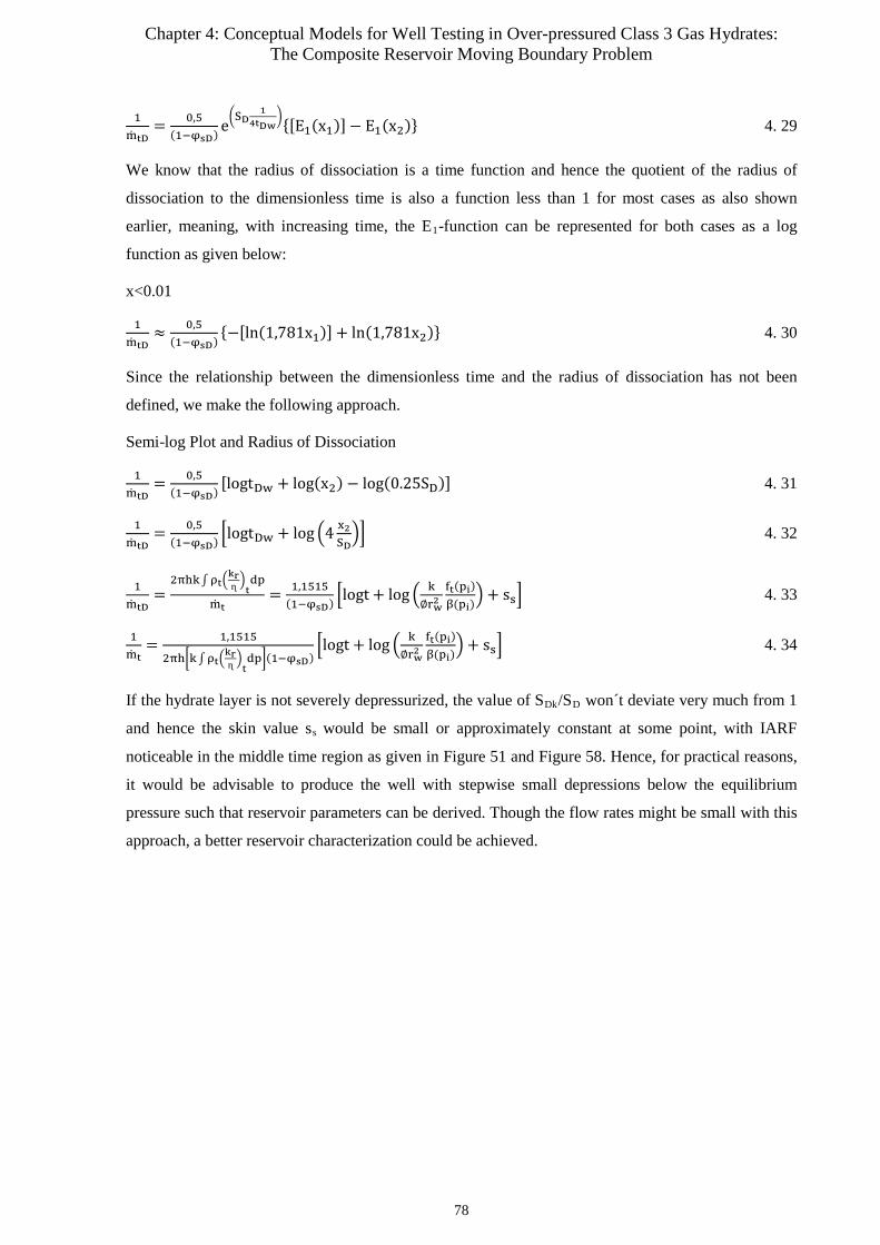
Chapter 4: Conceptual Models for Well Testing in Over-pressured Class 3 Gas Hydrates: The Composite Reservoir Moving Boundary Problem
1mtD
= 0,5(1−φsD) e�SD
14tDw
�{[E1(x1)]− E1(x2)} 4. 29
We know that the radius of dissociation is a time function and hence the quotient of the radius of
dissociation to the dimensionless time is also a function less than 1 for most cases as also shown
earlier, meaning, with increasing time, the E1-function can be represented for both cases as a log
function as given below:
x<0.01
1mtD
≈ 0,5(1−φsD)
{−[ln(1,781x1)] + ln(1,781x2)} 4. 30
Since the relationship between the dimensionless time and the radius of dissociation has not been
defined, we make the following approach.
Semi-log Plot and Radius of Dissociation
1mtD
= 0,5(1−φsD)
[logtDw + log(x2) − log(0.25SD)] 4. 31
1mtD
= 0,5(1−φsD) �logtDw + log �4 x2
SD�� 4. 32
1mtD
=2πhk∫ρt�
krɳ �t
dp
mt= 1,1515
(1−φsD) �logt + log � k∅rw2
ft(pi)β(pi)
� + ss� 4. 33
1mt
= 1,1515
2πh�k∫ρt�krɳ �t
dp�(1−φsD)�logt + log � k
∅rw2ft(pi)β(pi)
�+ ss� 4. 34
If the hydrate layer is not severely depressurized, the value of SDk/SD won´t deviate very much from 1
and hence the skin value ss would be small or approximately constant at some point, with IARF
noticeable in the middle time region as given in Figure 51 and Figure 58. Hence, for practical reasons,
it would be advisable to produce the well with stepwise small depressions below the equilibrium
pressure such that reservoir parameters can be derived. Though the flow rates might be small with this
approach, a better reservoir characterization could be achieved.
78

Chapter 4: Conceptual Models for Well Testing in Over-pressured Class 3 Gas Hydrates: The Composite Reservoir Moving Boundary Problem
Figure 58: Rate Transient Analysis in Over-pressured Gas Hydrates
The observed gradient from the semi-log plot is given by:
mlog = 1.1515
2πh(1−φsD)�k∫ρt�krɳ �t
dp� 4. 35
(1 − φsD) �k∫ρt �krɳ�t
dp� = 1.15152πhmlog
4. 36
Skin
ss,avg ≈� 1mt
�𝑡𝑡=1𝑠𝑠
mlog− log � k
∅rw2ft(pi)β(pi)
� 4. 37
As seen with the normally pressured gas hydrate reservoirs, the effective gas permeability can be
estimated from the mass balance approach thus:
kkrg∗ = kg∗ =[φPI(t)]g
mt[k∫ ft(p)dp] = 1
(1−φsD)[φPI(t)]g
mt
1,15152πhmlog
4. 38
Radius of Dissociation during Production
Deriving a clear gradient on the semi-log plot could be cumbersome; hence we use the average value
of skin as given above. This implies the use of this model only gives an approximation of the radius of
dissociation for any given time during IARF. From the total production time, the radius of dissociation
during IARF is given by:
ss,avg = log �rsD2
tDw� 4. 39
rs,avg ≈ �rw2[tDw]exp (2,303ss) = ��k∅ft(pi)β(pi)
tf� exp (2,303ss,avg) 4. 40
rs,avg ≈ rw𝑉𝑉(1.1515𝑠𝑠𝑠𝑠)√tDw 4. 41
-4
0
4
8
12
16
20
24
1E-01 1E+01 1E+03 1E+05 1E+07 1E+09 1E+11 1E+13 1E+15
1/ṁtD[-]
tDw[-]
RTA Semi-log Plot: IAR and CPIB
SDk/SD (≤1) = 0,1
SDk/SD (≤1) = 0,01
SDk/SD (≤1) = 0,001
79
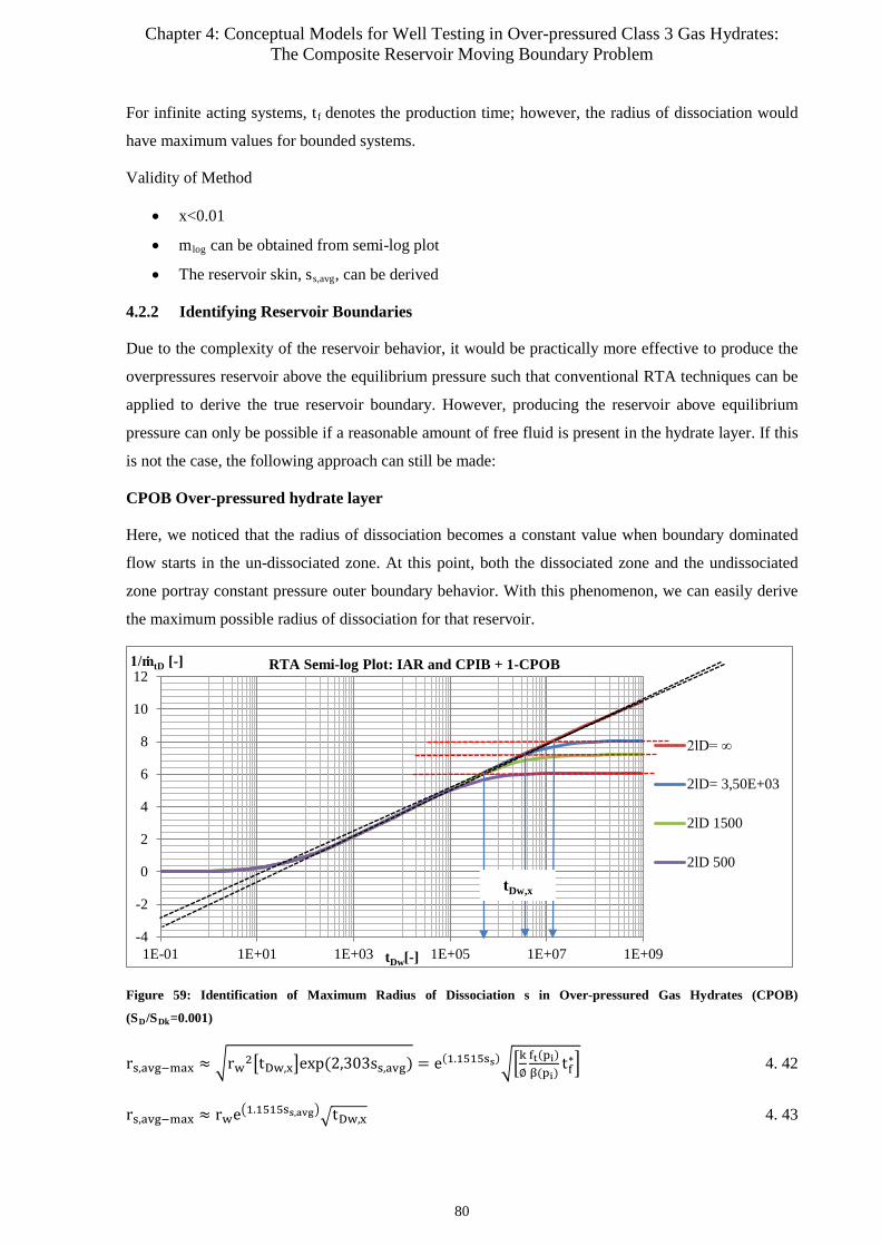
Chapter 4: Conceptual Models for Well Testing in Over-pressured Class 3 Gas Hydrates: The Composite Reservoir Moving Boundary Problem
For infinite acting systems, tf denotes the production time; however, the radius of dissociation would
have maximum values for bounded systems.
Validity of Method
• x<0.01
• mlog can be obtained from semi-log plot
• The reservoir skin, ss,avg, can be derived
4.2.2 Identifying Reservoir Boundaries
Due to the complexity of the reservoir behavior, it would be practically more effective to produce the
overpressures reservoir above the equilibrium pressure such that conventional RTA techniques can be
applied to derive the true reservoir boundary. However, producing the reservoir above equilibrium
pressure can only be possible if a reasonable amount of free fluid is present in the hydrate layer. If this
is not the case, the following approach can still be made:
CPOB Over-pressured hydrate layer
Here, we noticed that the radius of dissociation becomes a constant value when boundary dominated
flow starts in the un-dissociated zone. At this point, both the dissociated zone and the undissociated
zone portray constant pressure outer boundary behavior. With this phenomenon, we can easily derive
the maximum possible radius of dissociation for that reservoir.
Figure 59: Identification of Maximum Radius of Dissociation s in Over-pressured Gas Hydrates (CPOB)
(SD/SDk=0.001)
rs,avg−max ≈ �rw2�tDw,x�exp (2,303ss,avg) = e(1.1515ss)��k∅ft(pi)β(pi)
tf∗� 4. 42
rs,avg−max ≈ rwe�1.1515ss,avg��tDw,x 4. 43
-4
-2
0
2
4
6
8
10
12
1E-01 1E+01 1E+03 1E+05 1E+07 1E+09
1/ṁtD [-]
tDw[-]
RTA Semi-log Plot: IAR and CPIB + 1-CPOB
2lD= ∞
2lD= 3,50E+03
2lD 1500
2lD 500tDw,x
80

Chapter 4: Conceptual Models for Well Testing in Over-pressured Class 3 Gas Hydrates: The Composite Reservoir Moving Boundary Problem
NFB Over-pressured hydrate layer
The NFB problem in over-pressured gas hydrates is much more complex compared to the CPOB case.
As seen in Figure 56 and Appendix 13, the RTA of the model will depict two boundary dominated
flow periods. Coupled with the effect of dissociation and the moving boundary problem, serious
challenges can be encountered with the analysis. For this reason it is advisable at this level to apply
computer aided methods of analysis for such problems as the use of semi-log plots to estimate
reservoir parameters will not yield satisfactory results. Nonetheless, performing derivative plots for
reservoir diagnostics would be very beneficial in identifying the complex behavior of NFB over-
pressured gas hydrates as seen in Figure 56.
4.2.3 Type Curve Analysis
The conceptual models developed here for the over-pressured gas hydrates using the similarity
solutions ignored the effect of heat conduction such that the complexity of the model can be reduced.
With this assumption, solutions to the model were derived and hence a type curve method of analysis
can be proposed. It should be noted that as long as well test data depict skin response for a long period
of time, the reservoir could be considered as an over-pressured gas hydrate, which could also be
verified from temperature depressions (i.e. if the reservoir experiences no temperature depressions
when produced above the estimated equilibrium pressure). If this is the case, the over-pressured type
curve can be used for the matching process.
Required Plots
• (1−φsD)mtD
Versus tDwrsD
• 1mt
Versus t
• φPI(t) Versus t
Time Match
The time match points along the vertical are:
�tDwrsD
�MP
; tMP; � SDSDk
�MP
4. 44
Where,
tDw = tk∅rw2
ft(pi)β(pi)
From the match points, the dimensionless interlayer heat flux compressibility is derived thus:
[rsD]MP = tDw�tDwrsD
�MP
= k∅rw2
ft(pi)β(pi)
tMP
�tDwrsD�MP
4. 45
81
Chapter 4: Conceptual Models for Well Testing in Over-pressured Class 3 Gas Hydrates: The Composite Reservoir Moving Boundary Problem
[rs]MP = k∅rw
ft(pi)β(pi)
tMP
�tDwrsD�MP
4. 46
Rate Match
The match along the horizontal is given by:
�(1 − φsD)
mtD�MP
; �1
mt�MP
; [φPI(t)]g,MP
Where,
mtD(1−φsD) = mt
2πh�(1−φsD)k∫ρt�krɳ �t
dp� 4. 47
�(1 − φsD)k∫ρt �krɳ�t
dp�𝑀𝑀𝑀𝑀
=��1−φsD�mtD
�MP
2πh� 1mt�MP
4. 48
kkrg∗ (p) = [φPI(t)]g,MP �1mt�MP
�(1− φsD)k∫ρt �krɳ�t
dp�𝑀𝑀𝑀𝑀
4. 49
4.2.4 Rate Derivative Analysis
The derivative plot is basically used for diagnosis of the reservoir behavior and for a better view of the
different flow regimes and boundary responses.
Early Time Region
Unlike the normally pressured gas hydrates, the over-pressured gas hydrates show a characteristic skin
response due to dissociation and the increasing radius of dissociation.
IARF
As seen in Figure 51, IARF could be difficult to achieve if the hydrate dissociation is very significant;
however, the characteristic behavior during IARF is given by:
d� 1mtD
�
d�ln�tDwSD��
= f � SDSDk
,𝜑𝜑𝑠𝑠𝐷𝐷� 4. 50
Late Time IARF
d� 1mtD
�
d�ln�tDwSD��
= 0.5 4. 51
Boundary dominated Flow with 1-NFB (negligible heat conduction)
d� 1mtD
�
d�ln�tDwSD��
= f � SDSDk
,𝜑𝜑𝑠𝑠𝐷𝐷� 4. 52
82
Chapter 4: Conceptual Models for Well Testing in Over-pressured Class 3 Gas Hydrates: The Composite Reservoir Moving Boundary Problem
Reservoirs with NFB will depict the following responses:
• Double NFB Response: This would occur if the reservoir is produced long enough for the
reservoir pressure to drop below the equilibrium pressure for the given constant wellbore
pressure.
• Single NFB Response: This would occur if the reservoir is produced long enough till the NFB
is reached but the reservoir pressure is still above the equilibrium pressure.
Boundary dominated Flow with 1-CPOB (negligible heat conduction)
𝑈𝑈� 1mtD
�
𝑈𝑈�ln�tDwSD��
= 0 4. 53
The rate derivative shows a zero slope during boundary dominated flow.
83
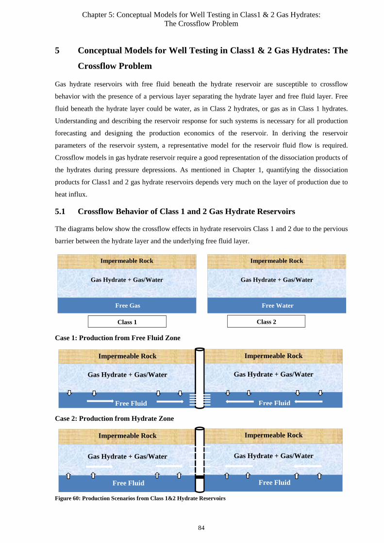
Chapter 5: Conceptual Models for Well Testing in Class1 & 2 Gas Hydrates: The Crossflow Problem
5 Conceptual Models for Well Testing in Class1 & 2 Gas Hydrates: The
Crossflow Problem
Gas hydrate reservoirs with free fluid beneath the hydrate reservoir are susceptible to crossflow
behavior with the presence of a pervious layer separating the hydrate layer and free fluid layer. Free
fluid beneath the hydrate layer could be water, as in Class 2 hydrates, or gas as in Class 1 hydrates.
Understanding and describing the reservoir response for such systems is necessary for all production
forecasting and designing the production economics of the reservoir. In deriving the reservoir
parameters of the reservoir system, a representative model for the reservoir fluid flow is required.
Crossflow models in gas hydrate reservoir require a good representation of the dissociation products of
the hydrates during pressure depressions. As mentioned in Chapter 1, quantifying the dissociation
products for Class1 and 2 gas hydrate reservoirs depends very much on the layer of production due to
heat influx.
5.1 Crossflow Behavior of Class 1 and 2 Gas Hydrate Reservoirs
The diagrams below show the crossflow effects in hydrate reservoirs Class 1 and 2 due to the pervious
barrier between the hydrate layer and the underlying free fluid layer.
Case 1: Production from Free Fluid Zone
Case 2: Production from Hydrate Zone
Figure 60: Production Scenarios from Class 1&2 Hydrate Reservoirs
Free Gas
Impermeable Rock
Gas Hydrate + Gas/Water
Class 1
Free Water
Impermeable Rock
Gas Hydrate + Gas/Water
Class 2
Free Fluid
Impermeable Rock
Gas Hydrate + Gas/Water
Free Fluid
Impermeable Rock
Gas Hydrate + Gas/Water
Free Fluid
Impermeable Rock
Gas Hydrate + Gas/Water
Free Fluid
Impermeable Rock
Gas Hydrate + Gas/Water
84
Chapter 5: Conceptual Models for Well Testing in Class1 & 2 Gas Hydrates: The Crossflow Problem
Different production scenarios have been identified and depicted in the above diagrams. The choice of
the production method will depend on various factors. One important aspect with the choice of
production will be the more energy efficient method. With a look at the hydrate reservoirs Class 1 and
2, it can be noticed that the fluid layer beneath the hydrate zone is more likely to possess a higher
permeability due to the absence of the hydrates in the pores. With such a case, it would be more
preferable to produce from the layer beneath the hydrate zone, as depletion here is faster. If we have
free water beneath the hydrate zone as in Class 2, production from the layer beneath the hydrate zone
would be predominantly water as in Coal Bed Methane reservoirs and could be called the dewatering
phase of the reservoir production, before the mobility of gas increases. For Class 1 with free gas
beneath the hydrate zone, production with Case 1 method will be predominantly gas.
To develop a more general equation, applicable for both Class 1 and Class 2, which also makes the use
of multiphase pseudo-pressure appropriate for crossflow problems, water and gas are assumed to be
present in both the hydrate layer and the layer beneath. With this assumption, mass conservation and
energy balance models could be used to describe flow in these reservoirs. Due to different outer
boundary conditions in the crossflow layer, various crossflow models have been developed
consequently. Most crossflow models are based on the extension of the non-leaky aquifer models.
Hantush and Jacob [43] first addressed the problem of crossflow using the leaky aquifer type models.
The influence of the fluid leakage from the confining layer (hydrate layer) to the producing layer (free
fluid layer) is highly dependent on the permeability and thickness of the hydrate formation as will be
shown later. The solutions presented by Hantush and Jacob [43] were derived for homogenous wells
and just ground water flow was considered; hence, linearization of the partial differential equation was
not necessary. However, dimensionless forms of the solutions have been presented by authors, which
could be seen in the works of Haefner [73] for different inner boundary conditions. The main
challenge with the crossflow problem in hydrate-capped reservoirs would be to linearize the equation
and represent in dimensionless forms, such that the boundary conditions could be modified and the
existing solutions in dimensionless form implemented. First, mass balance techniques are depicted for
the crossflow models.
Description of Pore Contents in Layers
Hydrate Layer (HL)
Considering the gas hydrate zone, we assume the pores are filled with three phases, namely: hydrate,
gas and water and the saturation is hence given by:
Sg + SH + Sw = VgVP
+ VHVP
+ VwVP
= Vg+VH+VwVp
= VpVp
= 1 5. 1
Considering the three phases in the reservoir, we could modify the storage term thus:
mt+∆t−mt ∆t
= ∆(ρ∗Vp)∆t
= ∆(ρ∗∅∗V)∆t
= ∆(ρg∗∅∗VSg)∆t
+ ∆(ρH∗∅∗VSH)∆t
+ ∆(ρw∗∅∗VSw)∆t
5. 2
85
Chapter 5: Conceptual Models for Well Testing in Class1 & 2 Gas Hydrates: The Crossflow Problem
This implies the rate of change of mass equation could be written in the form
mt+∆t−mt ∆t
= � mt+∆t−mt ∆t
�g
+ � mt+∆t−mt ∆t
�H
+ � mt+∆t−mt ∆t
�w
5. 3
As demonstrated in Appendix 1, Appendix 2, Appendix 3, the hydrate mass rate change could be
represented in terms of the dissociation components thus:
� mt+∆t−mt ∆t
�H
= ∆(ρH∗∅∗VSH)∆t
= � mt+∆t−mt ∆t
�w,H
+ � mt+∆t−mt ∆t
�g,H
5. 4
Free Fluid Layer (FFL)
Considering the free fluid zone, we assume the pores are filled with two phases, namely: gas and water
and the saturations are hence given by:
Sg + Sw = VgVP
+ VwVP
= Vg+VwVp
= VpVp
= 1 5. 5
Considering the two phases in the free fluid layer, we could modify the storage term thus:
mt+∆t−mt ∆t
= ∆(ρ∗Vp)∆t
= ∆(ρ∗∅∗V)∆t
= ∆(ρg∗∅∗VSg)∆t
+ ∆(ρw∗∅∗VSw)∆t
5. 6
This implies the rate of change of mass equation could be written in the form
mt+∆t−mt ∆t
= � mt+∆t−mt ∆t
�g
+ � mt+∆t−mt ∆t
�w
5. 7
Diffusivity Equation in Producing Layer (Layer 1)
In developing the equation, the hydrate dissociation rate due to heat conduction and convection should
be taking into consideration. Appendix 15 fully describes the derivation of the model.
Diffusivity Equation when producing from the Free Fluid Layer
∂2φD∂rD2
+ 1rD
∂φD ∂rD
− δD �∂[φD] layer2
∂zD�𝑧𝑧𝐷𝐷=1
= ω ∂φD∂tDwD
5. 8
The equation above is represented in Laplace domain thus:
∂2φ�D∂rD2
+ 1rD
∂φ�D ∂rD
− δD �∂[φ�D] layer2
∂zD�𝑧𝑧𝐷𝐷=1
= ωpφ�D 5. 9
Diffusivity Equation when producing from the Hydrate Layer
∂2φD∂rD2
+ 1rD
∂φD ∂rD
− �∂T𝑝𝑝𝐷𝐷∂z𝐷𝐷
�𝐶𝐶𝐶𝐶𝐶𝐶𝐶𝐶𝐶𝐶𝐶𝐶𝑘𝑘,𝑧𝑧𝐷𝐷=1
− δD �∂[φD] layer2
∂zD�𝑧𝑧𝐷𝐷=1
− δDθD �∂[φD] layer2
∂zD�𝑧𝑧𝐷𝐷=1
= ω ∂φD∂tDwD
5. 10
The diffusivity equation when producing from the hydrate layer can be similarly transformed in
Laplace domain as given below:
∂2φ�D∂rD2
+ 1rD
∂φ�D ∂rD
− �∂T�pD∂zD
�Caprock,zD=1
− δD �∂[φ�D] layer2
∂zD�zD=1
−δDθD �∂[φ�D] layer2
∂zD�zD=1
= ωpφ�D 5. 11
86
Chapter 5: Conceptual Models for Well Testing in Class1 & 2 Gas Hydrates: The Crossflow Problem
Diffusivity Equation for the Crossflow Layer (Layer 2)
�∂2φ�D∂zD
2 �layer2
= (1−ω)𝑝𝑝�φ�D�layer 2 5. 12
Mass Influx from Hydrate Layer in Free Fluid Layer
Since the hydrate layer is considered to be bounded at the top with a caprock, NFB is imposed at the
hydrate layer-caprock interface. Nonetheless, the endothermic dissociations favors heat inflow at this
interface when pressure propagation reaches the boundary. This effect is considered in the following
model:
NFB at top of Hydrate Layer
�∂[φD� ]layer2∂zD
�zD=1
= ��p[1−ω]Coth�(1− ∆zD)�p[1−ω]���p[1−ω]tanh�(1−∆zD)�p[1−ω]�+QpD�eD�
��p[1−ω]Coth�(1−∆zD)�p[1−ω]�+QpD�eD�� [φD� ]layer1 = Mi[φD� ]layer1 5. 13
Mass Influx from Free Fluid Layer in Hydrate Layer
The mass influx rate from the free fluid layer depends basically on the boundary condition imposed at
the bottom of the free fluid layer. Two boundary conditions have been considered in this work, for
which the mass influx rate is given by:
For CPOB at the bottom of the free fluid layer
�∂[φD� ]layer2∂zD
�zD=1
= ��p[1 −ω]Coth��p[1−ω](1 − ∆zD)��[φD� ]layer1 = 𝑀𝑀𝑖𝑖�φD��layer1
5. 14
For NFB at the bottom of the free fluid layer
�∂[φD� ]layer2∂zD
�zD=1
= ��p[1 −ω]tanh��p[1−ω](1 − ∆zD)��[φD� ]layer1 = 𝑀𝑀𝑖𝑖�φD��layer1
5. 15
We clearly see the difference in the NFB responses when producing from either one of the layers.
The final equations then take the form:
Final Model with Production from Hydrate Layer
∂2φ�D∂rD2
+ 1rD
∂φ�D ∂rD
− ��QpD� eD�
𝐶𝐶𝐶𝐶𝐶𝐶𝐶𝐶𝐶𝐶𝐶𝐶𝑘𝑘+ δD(1 + θD)Mi + ωp� φD� = 0 5. 16
Final Model with Production from Free Fluid Layer
∂2φ�D∂rD2
+ 1rD
∂φ�D ∂rD
− [δDMi + ωp]φD� = 0 5. 17
The models addressed here assume that flow in the producing layer is mainly horizontal and flow in
the overlain layer is mainly vertical. In case the hydrate layer is much more permeable compared to
the free fluid layer, production will be preferably done from the hydrate layer and the problem will be
handled analog. Coupled with the heat flux from the free fluid zone, more hydrate will be dissociated.
87
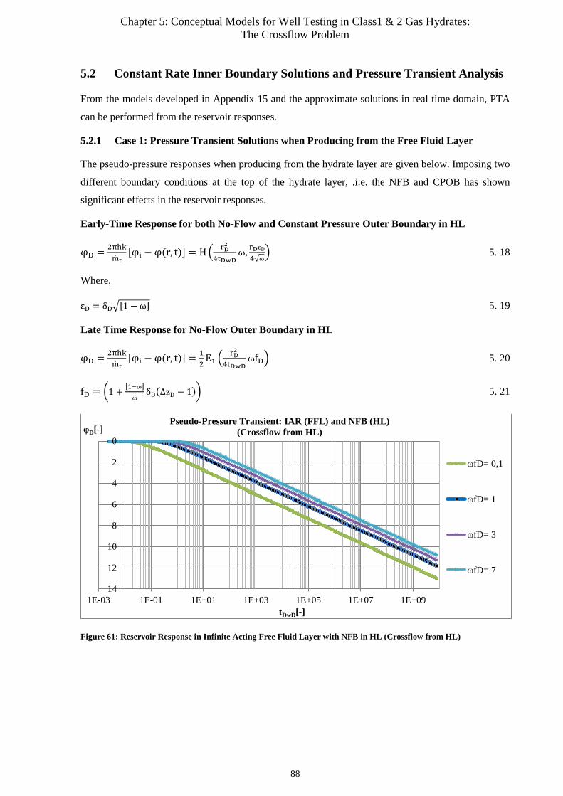
Chapter 5: Conceptual Models for Well Testing in Class1 & 2 Gas Hydrates: The Crossflow Problem
5.2 Constant Rate Inner Boundary Solutions and Pressure Transient Analysis
From the models developed in Appendix 15 and the approximate solutions in real time domain, PTA
can be performed from the reservoir responses.
5.2.1 Case 1: Pressure Transient Solutions when Producing from the Free Fluid Layer
The pseudo-pressure responses when producing from the hydrate layer are given below. Imposing two
different boundary conditions at the top of the hydrate layer, .i.e. the NFB and CPOB has shown
significant effects in the reservoir responses.
Early-Time Response for both No-Flow and Constant Pressure Outer Boundary in HL
φD = 2πhkmt
[φi − φ(r, t)] = H � rD2
4tDwDω, rDεD
4√ω� 5. 18
Where,
εD = δD�[1 −ω] 5. 19
Late Time Response for No-Flow Outer Boundary in HL
φD = 2πhkmt
[φi − φ(r, t)] = 12
E1 �rD2
4tDwDωfD� 5. 20
fD = �1 +[1−ω]ω
δD(∆zD − 1)� 5. 21
Figure 61: Reservoir Response in Infinite Acting Free Fluid Layer with NFB in HL (Crossflow from HL)
0
2
4
6
8
10
12
141E-03 1E-01 1E+01 1E+03 1E+05 1E+07 1E+09
φD[-]
tDwD[-]
Pseudo-Pressure Transient: IAR (FFL) and NFB (HL) (Crossflow from HL)
ωfD= 0,1
ωfD= 1
ωfD= 3
ωfD= 7
88
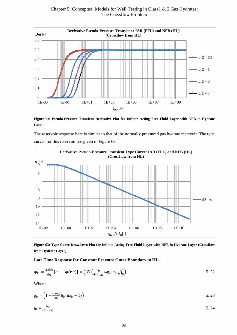
Chapter 5: Conceptual Models for Well Testing in Class1 & 2 Gas Hydrates: The Crossflow Problem
Figure 62: Pseudo-Pressure Transient Derivative Plot for Infinite Acting Free Fluid Layer with NFB in Hydrate
Layer
The reservoir response here is similar to that of the normally pressured gas hydrate reservoir. The type
curves for this reservoir are given in Figure 63.
Figure 63: Type Curve Drawdown Plot for Infinite Acting Free Fluid Layer with NFB in Hydrate Layer (Crossflow
from Hydrate Layer)
Late Time Response for Constant Pressure Outer Boundary in HL
φD = 2πhkmt
[φi − φ(r, t)] = 12
W � rD2
4tDwDωgD, rD�jD� 5. 22
Where,
gD = �1 + [1−ω]3ω
δD(∆zD − 1)� 5. 23
jD = δD(∆zD−1)
5. 24
0
0,1
0,2
0,3
0,4
0,5
0,6
1E-03 1E-01 1E+01 1E+03 1E+05 1E+07 1E+09
Der[-]
tDwD[-]
Derivative Pseudo-Pressure Transient : IAR (FFL) and NFB (HL) (Crossflow from HL)
ωfD= 0,1
ωfD= 1
ωfD= 3
ωfD= 7
0
2
4
6
8
10
12
141E-02 1E+00 1E+02 1E+04 1E+06 1E+08 1E+10
φD[-]
tDwD/ωfD[-]
Derivative Pseudo-Pressure Transient Type Curve: IAR (FFL) and NFB (HL) (Crossflow from HL)
rD= ∞
89

Chapter 5: Conceptual Models for Well Testing in Class1 & 2 Gas Hydrates: The Crossflow Problem
Figure 64: Pseudo-Pressure Transient Plot for Infinite Acting Free Fluid Layer with CPOB in Hydrate Layer
(Crossflow from Hydrate Layer)
Figure 65: Derivative Plot for Infinite Acting Free Fluid Layer with CPOB in Hydrate Layer (Crossflow from
Hydrate Layer)
5.2.2 Reservoir Parameters
For hydrate reservoirs with a no-flow outer boundary at the top, the influence of crossflow is
predominant in the early time period of production, which is however very short. The significance of
reservoir parameters in the dimensionless terms presented in the models earlier is now addressed.
Storativity Ratio
(1 −ω) =[av]𝑖𝑖
av��
ahah + av
��i
0
2
4
6
8
10
12
141E-02 1E+00 1E+02 1E+04 1E+06 1E+08 1E+10
φD[-]
tDwD/ωgD[-]
Pseudo-Pressure Transient: IAR (FFL) and CPOB (HL) (Crossflow from HL)
√jD 0,000001
√jD 0,0001
√jD 0,001
√jD 0,01
√jD 0,1
√jD 0,5
0
0,1
0,2
0,3
0,4
0,5
0,6
1E-02 1E+00 1E+02 1E+04 1E+06 1E+08 1E+10
ΔφD/Δ
ln(t
Dw
D/ω
g D)[
-]
tDwD/ωgD[-]
Derivative Pseudo-Pressure Transient: IAR (FFL) and CPOB (HL) (Crossflow from HL)
√jD 0,000001
√jD 0,0001
√jD 0,001
√jD 0,01
√jD 0,1
√jD 0,5
90

Chapter 5: Conceptual Models for Well Testing in Class1 & 2 Gas Hydrates: The Crossflow Problem
ω = [ah]𝑖𝑖ah
�� avah+av
��i 5. 25
ahav
= (1−ω)ω
5. 26
Interporosity Flow Coefficient
δD = rw2
∆z2∆z1
kv2kh1
5. 27
Dimensionless Early Time Interlayer Mass Flux Coefficient
εD = δD�[1 −ω] 5. 28
Dimensionless Interlayer Crossflow Compressibility (NFB in HL)
fD = �1 +[1−ω]ω
δD(∆zD − 1)� = �1 + ahav
rw2
∆z2∆z1
kv2kh1
(∆zD − 1)� 5. 29
With the above equation, we can conclude that the thicker the producing layer, the more insignificant
the effects of crossflow. Moreover, if the reservoir permeability of the free fluid layer is much higher
than the hydrate layer, which is also the precondition for producing from this layer and developing the
model, the influence of the dimensionless interlayer crossflow compressibility diminishes.
Dimensionless Interlayer Crossflow Storativity Compressibility Product
ωfD = [ω + (1 − ω)δD(∆zD − 1)] 5. 30
For hydrate reservoirs with much lower pressure conductivities with respect to the free fluid layer, the
storativity ratio is very small. As such, the dimensionless interlayer crossflow storativity
compressibility product could be less than 1, considering the interporosity flow coefficient is far less
than 1. In this case, the hydrate layer acts similar to a no-flow boundary for the free fluid layer and
hence the pressure depression in the free fluid layer is much higher as also seen in Figure 61. It should
however be emphasized that the dissociation of the hydrate layer would lead to an increase in the
pressure conductivity in the hydrate layer. With this increase, pressure depression in the hydrate layer
increases more rapidly and hence boundary dominated flow in the hydrate layer is faster achieved.
Dimensionless Interlayer Crossflow Compressibility (CPOB in HL)
gD = �1 + [1−ω]3ω
δD(∆zD − 1)� 5. 31
Dimensionless Interlayer Mass Flux Coefficient
jD = δD(∆zD−1)
5. 32
91
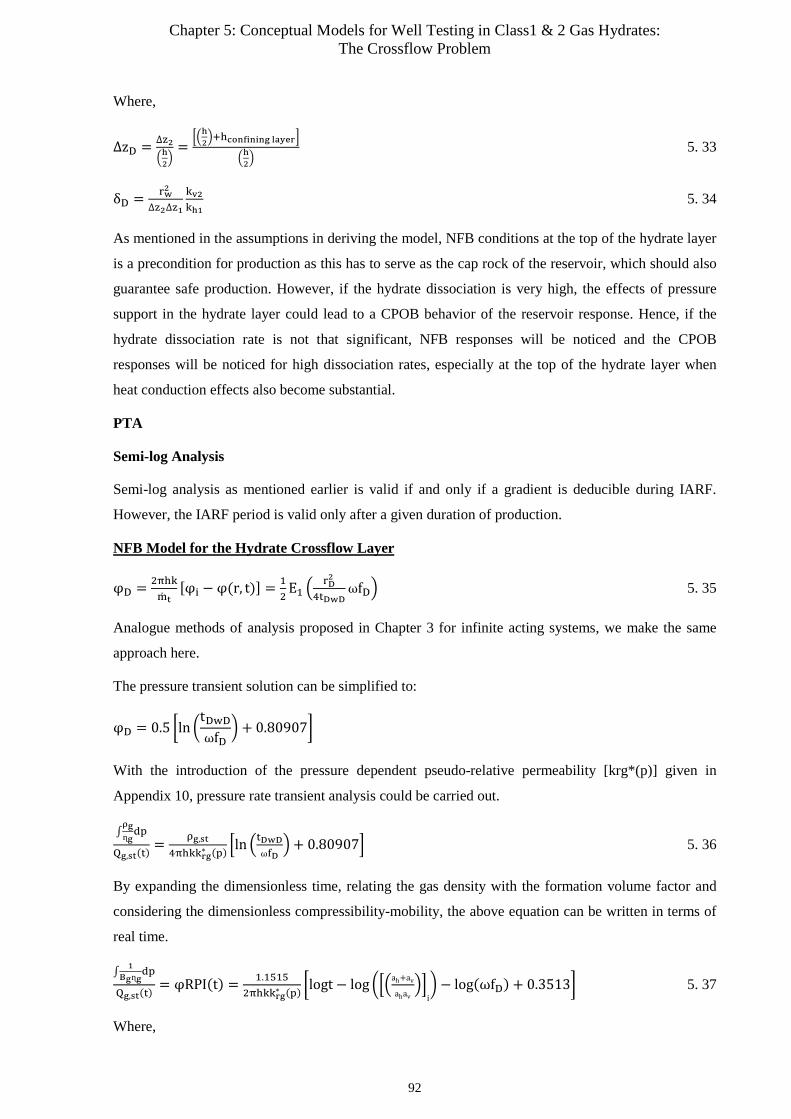
Chapter 5: Conceptual Models for Well Testing in Class1 & 2 Gas Hydrates: The Crossflow Problem
Where,
∆zD = ∆z2�h2�
=��h2�+hconfining layer�
�h2� 5. 33
δD = rw2
∆z2∆z1
kv2kh1
5. 34
As mentioned in the assumptions in deriving the model, NFB conditions at the top of the hydrate layer
is a precondition for production as this has to serve as the cap rock of the reservoir, which should also
guarantee safe production. However, if the hydrate dissociation is very high, the effects of pressure
support in the hydrate layer could lead to a CPOB behavior of the reservoir response. Hence, if the
hydrate dissociation rate is not that significant, NFB responses will be noticed and the CPOB
responses will be noticed for high dissociation rates, especially at the top of the hydrate layer when
heat conduction effects also become substantial.
PTA
Semi-log Analysis
Semi-log analysis as mentioned earlier is valid if and only if a gradient is deducible during IARF.
However, the IARF period is valid only after a given duration of production.
NFB Model for the Hydrate Crossflow Layer
φD = 2πhkmt
[φi − φ(r, t)] = 12
E1 �rD2
4tDwDωfD� 5. 35
Analogue methods of analysis proposed in Chapter 3 for infinite acting systems, we make the same
approach here.
The pressure transient solution can be simplified to:
φD = 0.5 �ln �tDwDωfD
� + 0.80907�
With the introduction of the pressure dependent pseudo-relative permeability [krg*(p)] given in
Appendix 10, pressure rate transient analysis could be carried out.
∫ρgɳgdp
Qg,st(t)= ρg,st
4πhkkrg∗ (p) �ln �tDwDωfD
�+ 0.80907� 5. 36
By expanding the dimensionless time, relating the gas density with the formation volume factor and
considering the dimensionless compressibility-mobility, the above equation can be written in terms of
real time.
∫ 1Bgɳg
dp
Qg,st(t)= φRPI(t) = 1.1515
2πhkkrg∗ (p) �logt − log ���ah+av
ahav��
i� − log(ωfD) + 0.3513� 5. 37
Where,
92
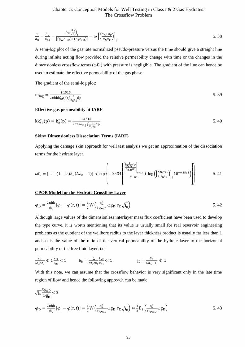
Chapter 5: Conceptual Models for Well Testing in Class1 & 2 Gas Hydrates: The Crossflow Problem
1𝐶𝐶ℎ
= SDah,i
=ρt,i�
krɳ �t
��ρwcT,w�+�ρgcT,g��= 𝜔𝜔 ��𝐶𝐶ℎ+𝐶𝐶𝑣𝑣
𝐶𝐶ℎ𝐶𝐶𝑣𝑣��𝑖𝑖 5. 38
A semi-log plot of the gas rate normalized pseudo-pressure versus the time should give a straight line
during infinite acting flow provided the relative permeability change with time or the changes in the
dimensionless crossflow terms (ωfD) with pressure is negligible. The gradient of the line can hence be
used to estimate the effective permeability of the gas phase.
The gradient of the semi-log plot:
mlog = 1.15152πhkkrg∗ (p)∫ 1
Bgɳgdp
5. 39
Effective gas permeability at IARF
kkrg∗ (p) = kg∗(p) = 1.15152πhmlog ∫
1Bgɳg
dp 5. 40
Skin= Dimensionless Dissociation Terms (IARF)
Applying the damage skin approach for well test analysis we get an approximation of the dissociation
terms for the hydrate layer.
ωfD = [ω + (1 − ω)δD(∆zD − 1)] ≈ exp
⎩⎪⎨
⎪⎧
−0.434
⎣⎢⎢⎢⎡�∫ 1Bgɳg
dp
Qg,st(t) �
𝑡𝑡=1𝑠𝑠mlog
+ log ���ah+avahav
��i10−0.3513�
⎦⎥⎥⎥⎤
⎭⎪⎬
⎪⎫
5. 41
CPOB Model for the Hydrate Crossflow Layer
φD = 2πhkmt
[φi − φ(r, t)] = 12
W � rD2
4tDwDωgD, rD�jD� 5. 42
Although large values of the dimensionless interlayer mass flux coefficient have been used to develop
the type curve, it is worth mentioning that its value is usually small for real reservoir engineering
problems as the quotient of the wellbore radius to the layer thickness product is usually far less than 1
and so is the value of the ratio of the vertical permeability of the hydrate layer to the horizontal
permeability of the free fluid layer, i.e.:
rw2
∆z2∆z1≪ 1 kv2
kh1< 1 δD = rw2
∆z2∆z1
kv2kh1
≪ 1 jD = δD(∆zD−1)
≪ 1
With this note, we can assume that the crossflow behavior is very significant only in the late time
region of flow and hence the following approach can be made:
�jDtDwDωgD
< 2
φD = 2πhkmt
[φi − φ(r, t)] = 12
W � rD2
4tDwDωgD, rD�jD� ≈
12
E1 �rD2
4tDwDωgD� 5. 43
93
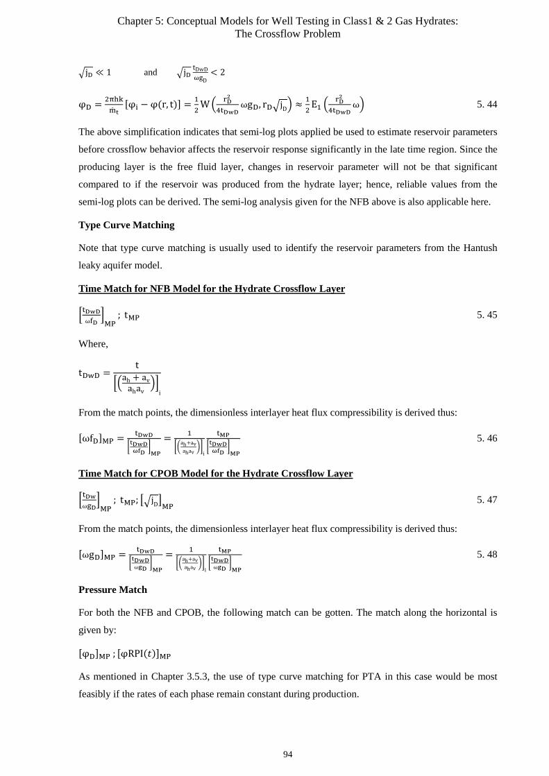
Chapter 5: Conceptual Models for Well Testing in Class1 & 2 Gas Hydrates: The Crossflow Problem
�jD ≪ 1 and �jDtDwDωgD
< 2
φD = 2πhkmt
[φi − φ(r, t)] = 12
W � rD2
4tDwDωgD, rD�jD� ≈
12
E1 �rD2
4tDwDω� 5. 44
The above simplification indicates that semi-log plots applied be used to estimate reservoir parameters
before crossflow behavior affects the reservoir response significantly in the late time region. Since the
producing layer is the free fluid layer, changes in reservoir parameter will not be that significant
compared to if the reservoir was produced from the hydrate layer; hence, reliable values from the
semi-log plots can be derived. The semi-log analysis given for the NFB above is also applicable here.
Type Curve Matching
Note that type curve matching is usually used to identify the reservoir parameters from the Hantush
leaky aquifer model.
Time Match for NFB Model for the Hydrate Crossflow Layer
�tDwDωfD
�MP
; tMP 5. 45
Where,
tDwD =t
��ah + avahav
��i
From the match points, the dimensionless interlayer heat flux compressibility is derived thus:
[ωfD]MP = tDwD
�tDwDωfD
�MP
= 1
��ah+avahav
��i
tMP
�tDwDωfD
�MP
5. 46
Time Match for CPOB Model for the Hydrate Crossflow Layer
�tDwωgD
�MP
; tMP; ��jD�MP 5. 47
From the match points, the dimensionless interlayer heat flux compressibility is derived thus:
[ωgD]MP = tDwD
�tDwDωgD
�MP
= 1
��ah+avahav
��i
tMP
�tDwDωgD
�MP
5. 48
Pressure Match
For both the NFB and CPOB, the following match can be gotten. The match along the horizontal is
given by:
[φD]MP ; [φRPI(𝑡𝑡)]MP
As mentioned in Chapter 3.5.3, the use of type curve matching for PTA in this case would be most
feasibly if the rates of each phase remain constant during production.
94
Chapter 5: Conceptual Models for Well Testing in Class1 & 2 Gas Hydrates: The Crossflow Problem
Derivatives
The derivatives of the type curve will show the following characteristics for the infinite acting
reservoir:
Early Time Region
No skin response
IARF (negligible crossflow)
d[φD]
d�ln�tDwDωfD
��= d[φD]
d�ln�tDwDωgD
��= 0.5 5. 49
IARF and high crossflow
d[φD]
d�ln�tDwDωfD
��= d[φD]
d�ln�tDwDωgD
��= 0 5. 50
5.2.3 Case 2: Pressure Transient Solutions and Analysis when Producing from the Hydrate
Layer
From the models developed in Appendix 15, the pseudo-pressure responses when producing from the
hydrate layer are given below. It should be noted that the combined effects of heat conduction from
the top of the hydrate layer and mass flux from the free fluid layer are considered in the model.
Early-Time Response for both No-flow Boundary and Constant Pressure Outer Boundary
(CPOB) in Crossflow
φD = 2πhkmt
[φi − φ(r, t)] = H � ωrD2
4tDwD, rDεD,2
4√ω� 5. 51
Where,
εD,2 = �𝑉𝑉D�FCD + δD(1 + θD)�[1−ω]� 5. 52
Late Time Period for Constant Pressure Outer Boundary (CPOB) in Crossflow Layer+Constant
Temperature Outer Boundary (CTOB) in Top Layer
φD = 2πhkmt
[φi − φ(r, t)] = 12
W � rD2
4tDwDωgD,2, rD�jD,2� 5. 53
Where,
gD,2 = �1 + 13ω�𝑉𝑉DFCD�∆zD,TL − 1� + δD(1 + θD)[1 −ω]�∆zD,BL − 1��� 5. 54
jD,2 = � δD(1+θD)�∆zD,BL−1�
+ 𝑈𝑈D�∆zD,TL−1�
� 5. 55
95

Chapter 5: Conceptual Models for Well Testing in Class1 & 2 Gas Hydrates: The Crossflow Problem
Figure 66: Drawdown Response in Infinite Acting Hydrate Layer with CPOB in Free Fluid Layer and CTOB in Top
Layer (Crossflow from Free Fluid Layer + Heat Conduction from Top Layer)
Late Time Period for No-flow Boundary (NFB) in Crossflow Layer+Constant Temperature
Outer Boundary (CTOB) in Top Layer (TL)
φD = 2πhkmt
[φi − φ(r, t)] = 12
W � rD2
4tDwDωfD,2, rD√YD� 5. 56
Where
fD,2 = �1 + 13ω��𝑉𝑉DFCD�∆zD,TL − 1� + 3�δD(1 + θD)(1 −ω)�∆zD,BL − 1����� 5. 57
YD = 𝑈𝑈D�∆zD,TL−1�
5. 58
Here, although the free fluid layer consists of a NFB, the reservoir response is much different from
when the reservoir is produced from the free fluid layer and the hydrate layer is a NFB layer. This is
solely due to the influence of heat conduction from the top layer which shows a significant influence
in the reservoir response during the late time period of production. We can hence conclude that when
producing from the hydrate layer in Class 1&2 gas hydrate reservoirs, we expect a much higher gas
recovery from the hydrate dissociation compared to Class 3 reservoirs, given the reservoirs have the
same petro-physical properties and provided the heat influx from the caprock is strong enough to
influence continuous hydrate dissociation. Note that the imposed CTOB at the caprock is an optimistic
model analogous to the kinetic model.
0
1
2
3
4
5
6
7
8
9
101E-03 1E-01 1E+01 1E+03 1E+05 1E+07 1E+09
φD[-]
tDwD/ωgD,2[-]
Pseudo-Pressure Transient: IAR (HL) with CPOB (FFL) and CTOB (TL) (Crossflow from Free Fluid Layer + Heat Conduction from Top Layer)
√γDk or √jD,2= 0,01
√γDk or √jD,2= 0,001
√γDk or √jD,2= 0,0001
√γDk or √jD,2= 0,1
√γDk or √jD,2= 0,5
96
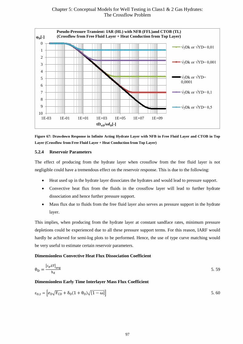
Chapter 5: Conceptual Models for Well Testing in Class1 & 2 Gas Hydrates: The Crossflow Problem
Figure 67: Drawdown Response in Infinite Acting Hydrate Layer with NFB in Free Fluid Layer and CTOB in Top
Layer (Crossflow from Free Fluid Layer + Heat Conduction from Top Layer)
5.2.4 Reservoir Parameters
The effect of producing from the hydrate layer when crossflow from the free fluid layer is not
negligible could have a tremendous effect on the reservoir response. This is due to the following:
• Heat used up in the hydrate layer dissociates the hydrates and would lead to pressure support.
• Convective heat flux from the fluids in the crossflow layer will lead to further hydrate
dissociation and hence further pressure support.
• Mass flux due to fluids from the free fluid layer also serves as pressure support in the hydrate
layer.
This implies, when producing from the hydrate layer at constant sandface rates, minimum pressure
depletions could be experienced due to all these pressure support terms. For this reason, IARF would
hardly be achieved for semi-log plots to be performed. Hence, the use of type curve matching would
be very useful to estimate certain reservoir parameters.
Dimensionless Convective Heat Flux Dissociation Coefficient
θD =�cp∆T�avg
hd 5. 59
Dimensionless Early Time Interlayer Mass Flux Coefficient
εD,2 = �𝑉𝑉D�FCD + δD(1 + θD)�[1−ω]� 5. 60
0
1
2
3
4
5
6
7
8
9
101E-03 1E-01 1E+01 1E+03 1E+05 1E+07 1E+09
φD[-]
tDwD/ωfD[-]
Pseudo-Pressure Transient: IAR (HL) with NFB (FFL)and CTOB (TL) (Crossflow from Free Fluid Layer + Heat Conduction from Top Layer)
√γDk or √YD= 0,01
√γDk or √YD= 0,001
√γDk or √YD= 0,0001
√γDk or √YD= 0,1
√γDk or √YD= 0,5
97
Chapter 5: Conceptual Models for Well Testing in Class1 & 2 Gas Hydrates: The Crossflow Problem
Dimensionless Interlayer Crossflow Compressibility
gD,2 = �1 + 13ω�𝑉𝑉DFCD�∆zD,TL − 1� + δD(1 + θD)[1 −ω]�∆zD,BL − 1��� 5. 61
Dimensionless Interlayer Mass Flux Coefficient
jD,2 = � δD(1+θD)�∆zD,BL−1�
+ 𝑈𝑈D�∆zD,TL−1�
� 5. 62
If the pressure depression in the hydrate layer and the interporosity flow coefficient are low, so will
the mass influx from the free fluid layer. Hence the influence of convective heat influx is negligible.
However, even with negligible mass flux from the free fluid layer during depressurization, we still
have conductive heat flux from the upper layer which assists in the dissociation process. This implies
the assumption of negligible dimensionless interlayer mass flux coefficient cannot be made with
certainty in this case.
Notice that both the dimensionless mass flux coefficient and the dimensionless interlayer crossflow
compressibility are functions of the storativity (energy used in the hydrate layer), the dimensionless
heat conductive flux coefficient (heat energy used from conduction), dimensionless convective heat
flux dissociation coefficient (energy used up from warmer fluids in the free fluid layer) and the
interporosity flow coefficient.
When the interporosity flow coefficient is negligible, the effects of mass flux from the free fluid layer
are also trivial and just heat conduction becomes very influential.
Dimensionless Interlayer Crossflow Compressibility
fD,2 = �1 + 13ω��𝑉𝑉DFCD�∆zD,TL − 1� + 3�δD(1 + θD)(1 −ω)�∆zD,BL − 1����� 5. 63
Dimensionless Interlayer Mass Flux Coefficient
YD = 𝑈𝑈D�∆zD,TL−1�
5. 64
The dimensionless interlayer mass flux coefficient for the NFB case is solely dependent on the heat
conduction term during late time production. However, if compared to producing from the free fluid
layer, the influence of heat conduction is better quantified and its influence represented in the model.
PTA
CPOB in Crossflow Layer and CTOB in Top Layer
As was done for the case of producing from the free fluid layer, we make simplifications of the model
for given ranges. With this note, we can assume that the crossflow behavior is not perceived in the
early-time region of flow and hence the following approach can be made for the given intervals below:
�jD,2tDwDωgD,2
< 2
98
Chapter 5: Conceptual Models for Well Testing in Class1 & 2 Gas Hydrates: The Crossflow Problem
φD = 2πhkmt
[φi − φ(r, t)] = 12
W � rD2
4tDwDωgD,2, rD�jD,2� ≈
12
E1 �rD2
4tDwDωgD,2� 5. 65
�jD,2 ≪ 1 and �jD,2tDwDωgD,2
< 2
φD = 2πhkmt
[φi − φ(r, t)] = 12
W � rD2
4tDwDωgD,2, rD�jD,2� ≈
12
E1 �rD2
4tDwDω� 5. 66
With the representation of the models in Ei-functions, the methods of analysis in 5.2.1 are also
applicable here.
NFB in Crossflow Layer and CTOB in Top Layer
�YDtDwDωfD,2
< 2
φD = 2πhkmt
[φi − φ(r, t)] = 12
W � rD2
4tDwDωfD,2, rD√YD� ≈
12
E1 �rD2
4tDwDωfD,2� 5. 67
√YD ≪ 1 and √YDtDwDωgD,2
< 2
φD = 2πhkmt
[φi − φ(r, t)] = 12
W � rD2
4tDwDωfD,2, rD√YD� ≈
12
E1 �rD2
4tDwDω� 5. 68
With the representation of the model in E1-functions, the methods of analysis in Chapter 3 are also
applicable here.
5.3 Constant Pressure Solutions and Rate Transient Analysis
Constant terminal solutions developed for the crossflow problem are now depicted with respect to the
layer of production.
5.3.1 Case 1: Producing from the Free Fluid Layer
Late Time Response for No-flow in HL
Dimensionless Pseudo-Pressure
φD = A �tDwDωfD
, rD� 5. 69
For tDwD/(ωfDrD²)>500
φD =E1�
rD2 ωfD4tDwD
�
E1�ωfD
4tDwD� 5. 70
Dimensionless Flowrate at Wellbore
mtD = G �tDwDωfD
� 5. 71
For tDwD/(ωfDrD²)>500
99
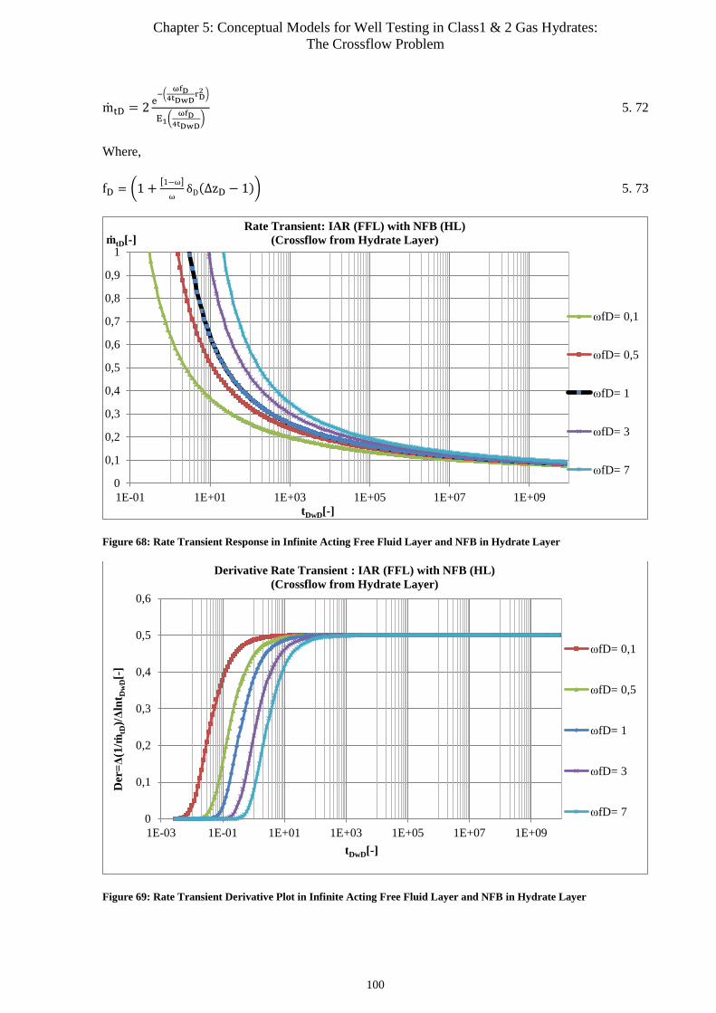
Chapter 5: Conceptual Models for Well Testing in Class1 & 2 Gas Hydrates: The Crossflow Problem
mtD = 2 e−�
ωfD4tDwD
rD2 �
E1�ωfD
4tDwD�
5. 72
Where,
fD = �1 + [1−ω]ω
δD(∆zD − 1)� 5. 73
Figure 68: Rate Transient Response in Infinite Acting Free Fluid Layer and NFB in Hydrate Layer
Figure 69: Rate Transient Derivative Plot in Infinite Acting Free Fluid Layer and NFB in Hydrate Layer
0
0,1
0,2
0,3
0,4
0,5
0,6
0,7
0,8
0,9
1
1E-01 1E+01 1E+03 1E+05 1E+07 1E+09
ṁtD[-]
tDwD[-]
Rate Transient: IAR (FFL) with NFB (HL) (Crossflow from Hydrate Layer)
ωfD= 0,1
ωfD= 0,5
ωfD= 1
ωfD= 3
ωfD= 7
0
0,1
0,2
0,3
0,4
0,5
0,6
1E-03 1E-01 1E+01 1E+03 1E+05 1E+07 1E+09
Der
=Δ(1
/ṁtD
)/Δln
t Dw
D[-
]
tDwD[-]
Derivative Rate Transient : IAR (FFL) with NFB (HL) (Crossflow from Hydrate Layer)
ωfD= 0,1
ωfD= 0,5
ωfD= 1
ωfD= 3
ωfD= 7
100

Chapter 5: Conceptual Models for Well Testing in Class1 & 2 Gas Hydrates: The Crossflow Problem
Due to NFB effects in the hydrate layer, crossflow will be trivial at the late time period of production
where the free fluid layer start depleting based on its reservoir content since the rate transient
responses converge as given in Figure 68. If the crossflow term for a given reservoir remains constant
throughout production, semi-log plots can be performed.
Late Time Period for CPOB in HL
Dimensionless Pseudo-Pressure
φD = Z �tDwωgD
, rD,�jD� 5. 74
For tDwωgD
�jD > 1
φD =W�
rD2 ωgD4tDwD
,rD�jD�
W� ωgD4tDwD
,�jD� 5. 75
Dimensionless Flowrate at Wellbore
mtD = G �tDwωgD
,�jD� 5. 76
For tDwωgD
jD > 1
mtD = 2
W� ωgD4tDwD
,�jD� 5. 77
Where,
gD = �1 + [1−ω]3ω
δD(∆zD − 1)� 5. 78
jD = δD(∆zD−1)
5. 79
Figure 70: Rate Transient Response in Infinite Acting Free Fluid Layer and CPOB in Hydrate Layer
00,10,20,30,40,50,60,70,80,9
1
1E-02 1E+00 1E+02 1E+04 1E+06 1E+08 1E+10
ṁtD[-]
tDwD/ωgD[-]
Rate Transient : IAR (FFL) with CPOB (HL) (Crossflow from Hydrate Layer)
√jD 1E-12
√jD 0,00001
√jD 0,0005
√jD 0,005
√jD 0,05
√jD 0,1
101
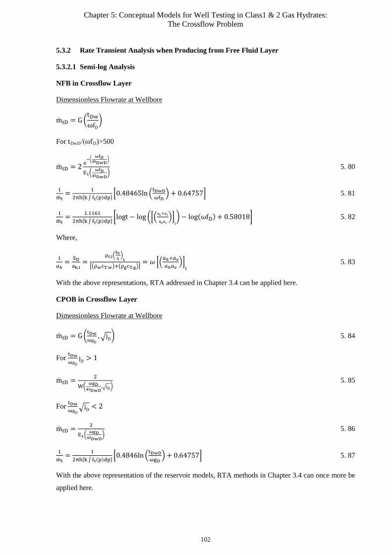
Chapter 5: Conceptual Models for Well Testing in Class1 & 2 Gas Hydrates: The Crossflow Problem
5.3.2 Rate Transient Analysis when Producing from Free Fluid Layer
5.3.2.1 Semi-log Analysis
NFB in Crossflow Layer
Dimensionless Flowrate at Wellbore
mtD = G �tDwωfD
�
For tDwD/(ωfD)>500
mtD = 2 e−�
ωfD4tDwD
�
E1�ωfD
4tDwD� 5. 80
1mt
= 12πh[k∫ ft(p)dp] �0.48465ln �tDwD
ωfD� + 0.64757� 5. 81
1mt
= 1.11612πh[k∫ ft(p)dp] �logt − log ���ah+av
ahav��
i� − log(ωfD) + 0.58018� 5. 82
Where,
1𝐶𝐶ℎ
= SDah,i
=ρt,i�
krɳ �t
��ρwcT,w�+�ρgcT,g��= 𝜔𝜔 ��𝐶𝐶ℎ+𝐶𝐶𝑣𝑣
𝐶𝐶ℎ𝐶𝐶𝑣𝑣��𝑖𝑖 5. 83
With the above representations, RTA addressed in Chapter 3.4 can be applied here.
CPOB in Crossflow Layer
Dimensionless Flowrate at Wellbore
mtD = G �tDwωgD
,�jD� 5. 84
For tDwωgD
jD > 1
mtD = 2
W� ωgD4tDwD
,�jD� 5. 85
For tDwωgD
�jD < 2
mtD = 2
E1�ωgD
4tDwD� 5. 86
1mt
= 12πh[k∫ ft(p)dp] �0.4846ln �tDwD
ωgD�+ 0.64757� 5. 87
With the above representation of the reservoir models, RTA methods in Chapter 3.4 can once more be
applied here.
102

Chapter 5: Conceptual Models for Well Testing in Class1 & 2 Gas Hydrates: The Crossflow Problem
5.3.2.2 Type Curve Matching
Time Match for NFB Model for the Hydrate Crossflow Layer
�tDwDωfD
�MP
; tMP 5. 88
Where,
tDwD =t
��ah + avahav
��i
From the match points, the dimensionless interlayer heat flux compressibility is derived thus:
[ωfD]MP = tDwD
�tDwDωfD
�MP
= 1
��ah+avahav
��i
tMP
�tDwDωfD
�MP
5. 89
Time Match for CPOB Model for the Hydrate Crossflow Layer
�tDwDωgD
�MP
; tMP; ��jD�MP 5. 90
From the match points, the dimensionless interlayer heat flux compressibility is derived thus:
[ωgD]MP = tDwD
�tDwDωgD
�MP
= 1
��ah+avahav
��i
tMP
�tDwDωgD
�MP
5. 91
Rate Match
For both the NFB and CPOB, the following match can be gotten. The match along the horizontal is
given by:
�1
mtD�MP
; �1
mt�MP
; [φPI(t)]g,MP
Similarly, the RTA methods in Chapter 3.4 can once more be applied here.
5.3.2.3 Derivatives
The derivatives of the type curves will show the following characteristics for the infinite acting
reservoir:
Early Time Region
No skin response
IARF (negligible crossflow)
d� 1mtD
�
d�ln�tDwDωfD
��=
d� 1mtD
�
d�ln�tDwDωgD
��= 0.5 5. 92
103
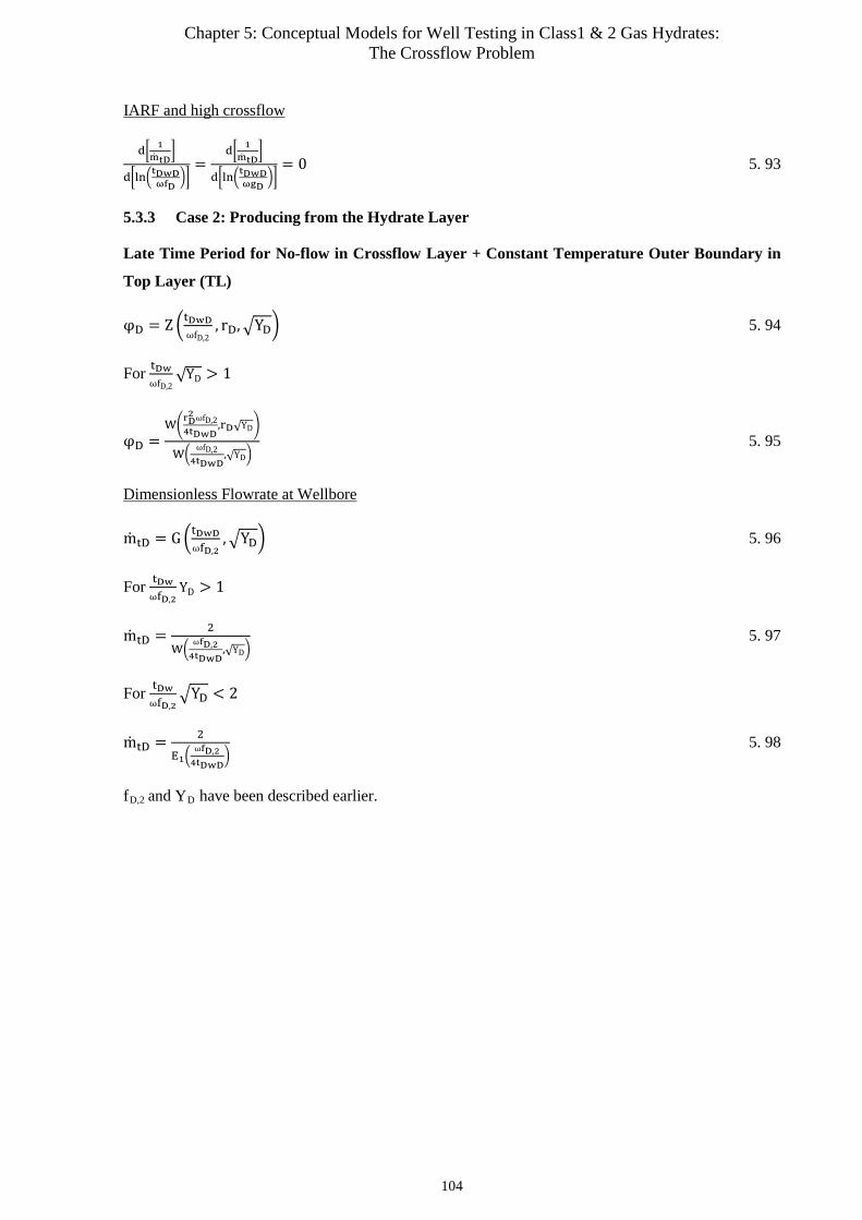
Chapter 5: Conceptual Models for Well Testing in Class1 & 2 Gas Hydrates: The Crossflow Problem
IARF and high crossflow
d� 1mtD
�
d�ln�tDwDωfD
��=
d� 1mtD
�
d�ln�tDwDωgD
��= 0 5. 93
5.3.3 Case 2: Producing from the Hydrate Layer
Late Time Period for No-flow in Crossflow Layer + Constant Temperature Outer Boundary in
Top Layer (TL)
φD = Z �tDwDωfD,2
, rD,�YD� 5. 94
For tDwωfD,2
√YD > 1
φD =W�
rD2 ωfD,24tDwD
,rD√YD�
W�ωfD,2
4tDwD,√YD�
5. 95
Dimensionless Flowrate at Wellbore
mtD = G �tDwDωfD,2
,�YD� 5. 96
For tDwωfD,2
YD > 1
mtD = 2
W�ωfD,24tDwD
,√YD� 5. 97
For tDwωfD,2
�YD < 2
mtD = 2
E1�ωfD,24tDwD
� 5. 98
fD,2 and YD have been described earlier.
104

Chapter 5: Conceptual Models for Well Testing in Class1 & 2 Gas Hydrates: The Crossflow Problem
Figure 71: Rate Transient Response in Infinite Acting Hydrate Layer with NFB in Free Fluid Layer and CTOB in
Top Confining Layer
Late Time Period for Constant Outer Pressure in Crossflow Layer+ Constant Temperature
Outer Boundary in Top
Dimensionless Pseudo-Pressure
φD = Z �tDwDωgD,2
, rD,�jD,2� 5. 99
For tDwωgD,2
�jD,2 > 1
φD =W�
rD2 ωgD,24tDwD
,rD�jD,2�
W�ωgD,24tDwD
,�jD,2� 5. 100
Dimensionless Flowrate at Wellbore
mtD = G � tDwωgD,2
,�jD,2� 5. 101
For tDwωgD,2
jD,2 > 1
mtD = 2
W�ωgD,24tDwD
,�jD,2� 5. 102
For tDwωfD,2
�jD,2 < 2
mtD = 2
E1�ωfD,24tDwD
� 5. 103
gD,2 and jD,2 have been described earlier.
0
0,1
0,2
0,3
0,4
0,5
0,6
0,7
0,8
0,9
1
1E+00 1E+02 1E+04 1E+06 1E+08 1E+10
ṁtD[-]
tDwD/ωfD,2[-]
Rate Transient: IAR (HL) with NFB (FFL) and CTOB (TL) (Crossflow from Free Fluid Layer + Heat Conduction from Top Layer)
√γDk or √YD= 0,0001
√γDk or √YD= 0,001
√γDk or √YD= 0,01
√γDk or √YD= 0,1
√γDk or √YD= 0,2
105
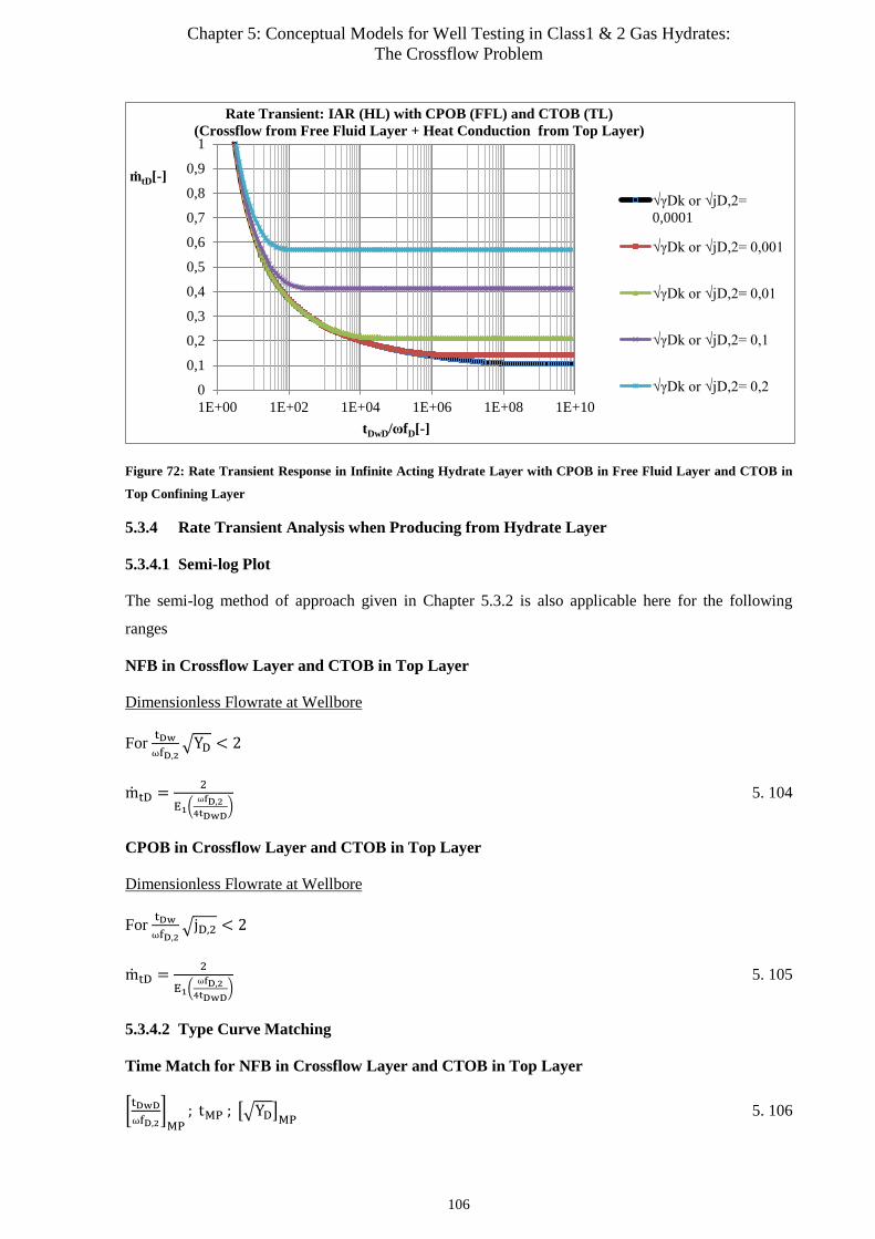
Chapter 5: Conceptual Models for Well Testing in Class1 & 2 Gas Hydrates: The Crossflow Problem
Figure 72: Rate Transient Response in Infinite Acting Hydrate Layer with CPOB in Free Fluid Layer and CTOB in
Top Confining Layer
5.3.4 Rate Transient Analysis when Producing from Hydrate Layer
5.3.4.1 Semi-log Plot
The semi-log method of approach given in Chapter 5.3.2 is also applicable here for the following
ranges
NFB in Crossflow Layer and CTOB in Top Layer
Dimensionless Flowrate at Wellbore
For tDwωfD,2
�YD < 2
mtD = 2
E1�ωfD,24tDwD
� 5. 104
CPOB in Crossflow Layer and CTOB in Top Layer
Dimensionless Flowrate at Wellbore
For tDwωfD,2
�jD,2 < 2
mtD = 2
E1�ωfD,24tDwD
� 5. 105
5.3.4.2 Type Curve Matching
Time Match for NFB in Crossflow Layer and CTOB in Top Layer
�tDwDωfD,2
�MP
; tMP ; ��YD�MP 5. 106
0
0,1
0,2
0,3
0,4
0,5
0,6
0,7
0,8
0,9
1
1E+00 1E+02 1E+04 1E+06 1E+08 1E+10
ṁtD[-]
tDwD/ωfD[-]
Rate Transient: IAR (HL) with CPOB (FFL) and CTOB (TL) (Crossflow from Free Fluid Layer + Heat Conduction from Top Layer)
√γDk or √jD,2= 0,0001
√γDk or √jD,2= 0,001
√γDk or √jD,2= 0,01
√γDk or √jD,2= 0,1
√γDk or √jD,2= 0,2
106
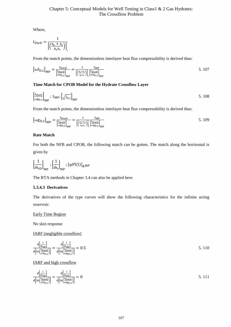
Chapter 5: Conceptual Models for Well Testing in Class1 & 2 Gas Hydrates: The Crossflow Problem
Where,
tDwD =t
��ah + avahav
��i
From the match points, the dimensionless interlayer heat flux compressibility is derived thus:
�ωfD,2�MP = tDwD
�tDwDωfD,2
�MP
= 1
��ah+avahav
��i
tMP
�tDwDωfD,2
�MP
5. 107
Time Match for CPOB Model for the Hydrate Crossflow Layer
�tDwDωgD,2
�MP
; tMP; ��jD,2�MP 5. 108
From the match points, the dimensionless interlayer heat flux compressibility is derived thus:
�ωgD,2�MP = tDwD
�tDwDωgD,2
�MP
= 1
��ah+avahav
��i
tMP
�tDwDωgD,2
�MP
5. 109
Rate Match
For both the NFB and CPOB, the following match can be gotten. The match along the horizontal is
given by
�1
mtD�MP
; �1
mt�MP
; [φPI(t)]g,MP
The RTA methods in Chapter 3.4 can also be applied here.
5.3.4.3 Derivatives
The derivatives of the type curves will show the following characteristics for the infinite acting
reservoir:
Early Time Region
No skin response
IARF (negligible crossflow)
d� 1mtD
�
d�ln�tDwDωfD,2
��=
d� 1mtD
�
d�ln�tDwDωgD,2
��= 0.5 5. 110
IARF and high crossflow
d� 1mtD
�
d�ln�tDwDωfD,2
��=
d� 1mtD
�
d�ln�tDwDωgD,2
��= 0 5. 111
107
Chapter 6: Summary and Outlook
6 Summary and Outlook
6.1 Summary
Conceptual models have been developed for Class 1, 2 and 3 gas hydrate reservoir and the reservoir
responses under different flowing conditions illustrated. It has been clearly shown that crossflow and
heat conduction effects in the hydrates can be taking into account in conceptual models as long as the
MBM pseudo-pressure is used and the temperature dependence on pressure can be characterized using
the Clausius-Clapeyron-Type hydrate equilibrium models. As depicted earlier, the characterization of
the gas hydrate reservoir is very complex due to the numerous parameters required to be identified.
However, the use of dimensionless parameters reduces the number of unknowns required for the
reservoir characterization.
6.1.1 Class 3-Normally Pressured Gas Hydrates
The main advantage of producing from normally pressured gas hydrate reservoirs would be the
reservoir pressure being considered to be approximately equal to the equilibrium pressure. In this case,
every pressure depression below the reservoir pressure dissociates the hydrates; hence, a much higher
recovery would be expected compared to the over-pressured gas hydrates. The absence of a pervious
free fluid layer beneath the hydrates excludes mass crossflow from the bottom layer but however
favors heat crossflow from both the top and bottom layers as a result of the endothermic hydrate
dissociation. The influence of heat influx, though a slow process, could be very significant for long-
term production scenarios as the negative rate declines could be noticed as the hydrate dissociation
rate increases. The following important aspects can further summarize the Normally Pressured Class 3
gas hydrate reservoirs as addressed in this work:
• The energy components responsible for hydrate dissociation in this reservoir are the heat
stored in the hydrate layer and the heat influx through conduction from the confining layers.
• Conceptual reservoir testing models have been developed for normally pressured Class 3 gas
hydrate reservoirs by rigorously combining mass and energy balance techniques.
• The dimensionless temperature conductivity introduced in this work gives the relationship
between the temperature and pressure conductivity in the confining and producing layers
respectively. With this approach, the rate of heat influx with respect to producing layer is
quantified. For reservoirs with high permeabilities, the pressure conductivity is much higher
than the heat influx rate; hence hydrate dissociation is slower in this case.
• Due to decreasing temperature with decreasing depth, as given by the geothermal profile,
pseudo-no-flow temperature boundaries would better describe the heat influx rate from the cap
rock whereas constant temperature outer boundary conditions would be more suitable for the
underlain layer due to increasing temperatures with increasing depths as also given by the
geothermal profile. The solutions presented in Laplace domain coupled with the Laplace
108
Chapter 6: Summary and Outlook
domain well test model identification methods address the effects of the different boundary
conditions. However, the solutions in real time domain adopted the constant temperature outer
boundary as an optimistic approach similar to the kinetic model, which depicts continuous
hydrate dissociation.
• Constant terminal rate and constant terminal pressure solutions and responses for the normally
pressured Class 3 gas hydrates have been depicted using dimensionless parameters.
• The solutions to the diffusivity problem are represented in terms of dimensionless mass rate
and dimensionless multiphase pseudo-pressures, developed using the mass balance model
(MBM).
• The use of the dimensionless mass rates and dimensionless multiphase pseudo-pressures
provides a huge advantage in the analysis, especially when performing RTA as mass
conservation can be verified for type curve matching techniques.
• Semi-log plots of pseudo-pressure normalized rates versus time have been used in the
estimation of the reservoir parameters in normally pressured Class 3 gas hydrates for specific
reservoir responses. It should however be strongly emphasized that the use of semi-log plots is
very limited due to the complex reservoir response, especially when hydrate dissociation is
significant.
• Type curve matching techniques for the normally pressured gas hydrates have been developed
for the derivation of the dimensionless parameters responsible for the hydrate dissociation in
this gas hydrate reservoir type by applying the Hantush et al. [43] well functions.
• The Bourdet [51] diagnostic (derivative) plots have been performed for the reservoir responses
to derive the theoretical characteristic behavior of the reservoir.
• The influence of heat conduction from the confining layers could have as significant effect of
the rate or pressure transient due to the increase in hydrate dissociation hence supplementary
pressure support.
• Boundary effects on the reservoir responses have been identified with semi-log and derivative
methods of identifying and estimating the distance to the reservoir boundary for instances with
reduced heat influx rates.
• The Bourgeois and Horne [25] Laplace domain well test model recognition method has been
applied to the exact solution in Laplace domain, including diagnostic plots in the Appendices,
which also gives a more explicit image of the complex reservoir behavior.
6.1.2 Class 3-Overpressured Gas Hydrates
Over-pressured gas hydrate reservoirs with reservoir pressures above the equilibrium pressures are
much more complex in behavior, mainly due to the moving boundary problem which results in a skin
response as seen on the derivative plots in this work. The reservoir model depicts two distinct zones,
109
Chapter 6: Summary and Outlook
analogous to composite reservoir models seen in conventional reservoir; however, the derivation of the
dissociation radius is another hurdle to overcome. The analytical solutions developed here for the
model using the similarity variable method neglect the effect of heat influx due to conduction such that
the complexity of the problem is reduced. Nonetheless, the solutions to the problem considering the
heat conduction have been developed in Laplace domain which still requires the use of numerical
inverse transforms to develop the solutions in time domain but have not been further addressed in this
work. However, Laplace domain well test model recognition methods have been fully addressed to
depict the reservoir response and aid in the characterization of these reservoirs. Most importantly, for
the development of the conceptual models for such a reservoir, mass conservation must be defined at
the dissociation front. In addition, the pressure propagation model for both the dissociated and
undissociated zone must be equal at the dissociation front. With these conditions, the radius of
dissociation can be derived for which both conditions hold, as shown in the models developed here.
For over-pressured gas hydrate reservoirs with a CPOB, just part of the reservoir can be dissociated as
long as pressure propagation has reached the reservoir boundary and boundary dominated flow is felt.
At this point, the wellbore, the dissociation front and the exterior boundary of the undissociated zone
all experience constant pressure boundary conditions. Pressure propagation stops and so does the
radius of dissociation. The total mass rate at both the wellbore and the dissociation front remain
constant with time as a result of the replenishment or pressure support at the exterior CPOB. With a
NFB at the exterior of the reservoir, quite a different phenomenon is seen. Here, the entire hydrate
reservoir could be dissociated as no pressure support at the reservoir exterior boundary is characterized
here. However, the undissociated zone first reaches the NFB and a reservoir pressure decline is
experienced although the dissociated zone is still in the transient flow regime. Due to this effect the
wellbore flow rate depicts a first boundary dominated decline while the dissociation radius further
increases. When the dissociation front reaches the NFB, the entire dissociated zone exhibits a second
boundary dominated responses as the average pressure drops below the equilibrium pressure. The
reservoir then behaves similarly to the normally pressured gas hydrate reservoir. The characteristic
behavior of these reservoirs is summarized in the type curve derivative or diagnostic responses in
Table 5. The following important aspects can further summarize the Over-Pressured Class 3 gas
hydrate reservoirs as depicted in this work:
• Like in normally-pressured Class 3 gas hydrates, the energy components responsible for
hydrate dissociation in this reservoir are the heat stored in the hydrate layer and the heat influx
through conduction from the confining layers.
• The moving boundary problem depicts a characteristic skin response from diagnostic plots,
which is not seen in the normally pressured Class 3 gas hydrate reservoirs, which is due to the
difference in the storativity of the dissociated and undissociated zones coupled with the
transient radius of dissociation.
110
Chapter 6: Summary and Outlook
• Reservoir boundaries have a significant effect on the moving boundary problem especially
with the presence no-flow boundaries.
• Constant pressure outer boundaries limit the extent to which the hydrates will dissociate; i.e.
only partial hydrate dissociation is possible.
• In the presence of no-flow boundaries, the reservoir depicts a characteristic double no-flow
boundary behavior due to the undissociated region reaching the no-flow boundary before the
entire reservoir is dissociated and depict a second no-flow boundary response.
• The application of semilog plots for such a case is very limited; especially if the dissociation
rate is high or the pressure depression at the wellbore is very significant.
• Derivative or diagnostic plots on the other hand are very vital in such cases as the skin effect
and the double no-flow boundary response can been easily identified.
• Type curve matching methods have been developed to estimate reservoir parameters for the
moving boundary problem.
• The Bourgeois and Horne [25] Laplace domain well test model recognition method have also
been applied to the exact solution in Laplace domain, including diagnostic plots for a better
view of the reservoir responses.
6.1.3 Class 1 and 2 Gas Hydrates
Class 1 and 2 gas hydrates reservoirs have been described as hydrate reservoirs demarcated from a free
fluid beneath the hydrate layer owing to the geothermal gradient or hydrate equilibrium conditions.
The crossflow problem in such a reservoir is the main issue to address here, coupled with the
determining factors for hydrate dissociation. As has been addressed in this work, the heat sources
responsible for hydrate dissociation when producing from the hydrate layer are heat stored in the
reservoir, heat conduction from the hydrate top layer (cap rock) and heat influx from the warm fluid in
the free fluid layer beneath the hydrates. All these factors accelerate the dissociation of the hydrates,
provided the reservoir is produced from the hydrate layer and hence the gas recovery factor for such a
production scenario could be much faster. The influence of heat conduction can be addressed similar
to the Class 3 gas hydrates for this case.
If the hydrate reservoir is produced from the free fluid layer, just heat stored in the hydrate layer and
heat influx due to heat conduction from the cap rock are responsible for the dissociation process.
When producing from the free fluid layer, heat conduction only starts when pressure depression in the
hydrate layer has reached the vertical outer boundary, i.e. the hydrate layer-cap rock interface. This
implies this will occur in the late time period of production. When hydrates dissociate at the vertical
outer boundary, this will depict a pressure support which if strong enough, will enable zero pressure
depressions at the vertical outer boundary. With the identification of these phenomena, a constant
pressure outer boundary can be imposed at the boundary and the influence of heat conduction
addressed in the crossflow model. This implies if the reservoir is produced from the free fluid layer,
111
Chapter 6: Summary and Outlook
CPOB response will only be seen if hydrate dissociation at the vertical outer boundary becomes
significant, provided the free fluid layer is not bounded in the horizontal by another CPOB. The
bounded reservoir models for the crossflow behavior have also been developed in Laplace domain
which can be transformed in real time domain using a suitable numerical inversion method but have
not been addressed further in this work. The characteristic behavior of these reservoirs is summarized
in the type curve derivative or diagnostic responses in Table 5.
The following important aspects can further summarize the Class 1 & 2 gas hydrate reservoirs as
depicted in this work:
• Since the two layers (free fluid and hydrate layer) are separated at the equilibrium point, they
can be considered as normally pressured, i.e. the reservoir pressure is approximately equal to
the equilibrium pressure.
• Production from one of the layers can result to crossflow.
Production Scenario 1: Producing from Hydrate Layer
• When producing from the hydrate layer, the heat energy balance for the hydrate dissociation
has to account for the heat conduction from the cap rock, the heat stored in the hydrate layer
and the heat from the warmer fluids in the free fluid layer moving into the hydrate layer as a
result of crossflow.
• The hydrate dissociation would be much faster when producing from the hydrate layer as
compared to the normally pressured Class 3 due to the supplementary heat source from the
crossflow fluids.
• Constant terminal rate methods can be very tedious for such a production scenario due to the
constant increase in pressure from dissociation, which could further result to a zero depression
at the sandface. This could make pressure transient analysis very cumbersome, especially with
significant changes in fractional flow.
• Constant terminal pressure on the other hand could be more beneficial as the wellbore pressure
would be maintained constant and the flow rates would increase significantly.
• Semi-log plots can be made only when the dissociation of crossflow effects are still at
minimum.
• Diagnostic plots are still a powerful tool in identifying the flow regimes and reservoir
characterization.
• Type curve matching techniques can be used to estimate reservoir parameters.
• The Bourgeois and Horne (1993) Laplace domain well test model recognition method have
also been applied to the exact solution in Laplace domain.
Production Scenario 2: Producing from Free Fluid Layer
112
Chapter 6: Summary and Outlook
• When producing from the free fluid layer, the heat energy balance for the hydrate dissociation
has to account for the heat conduction from the cap rock and the heat stored in the hydrate
layer.
• The heat energy due to conduction from the top layer occurs only during late time production
periods when pressure depression has reached the outer boundary of the hydrate layer and a
temperature depression exists due to dissociation.
• The complexity of developing the model can be addressed by considering the dissociation of
the hydrates at the outer boundary in the late time period as a pressure support , which if
strong enough can lead to constant pressure at the outer boundary of the hydrate layer.
• Semi-log plots can also be made here if and only if the crossflow effects are still at minimum.
• Derivative plots can be used to better identify flow regimes and reservoir characterization.
• The Bourgeois and Horne [25] Laplace domain well test model recognition method have also
been applied to the exact solution in Laplace domain.
To conclude, the hydrate dissociation is a pressure or mass source and hence tends to replenish
pressure or rate declines during production. For this reason, most of the reservoir response models
with significant hydrate dissociation depict a similar characteristic behavior. However, the parameters
influencing such a behavior are different for each reservoir type as seen in this work using the
equilibrium model. Hence, knowledge about the reservoir in question is essential for qualitative
analysis of rate / pressure data. The well testing models developed here did not consider wellbore
storage or mechanical skin damage effects on the reservoir behavior such that the true reservoir
responses can be identified, after which other parameters can be addressed and incorporated in the
model.
113

Chapter 6: Summary and Outlook
Table 5: Summary of Characteristic Behavior of Gas Hydrate Reservoirs from Type Curve Derivatives in Real Time Domain (Total System Response)
Type Curve Derivative and Skin
Type Curve Derivative and IARF
Type Curve Derivative and 1-CPOB
Type Curve Derivative and 1-NFB
Class 3 Normally Pressured Gas Hydrates (Pi=Peq) • Heat Stored in Reservoir
Considered • Heat Conduction
Considered
No Skin
0.5 (1xmlog)
with negligible heat flux at middle time region
0
with high heat flux at middle time region
0
with negligible heat flux at late time region
Not Applicable
with high heat flux, pressure transient does not
reach boundary
1 (2xmlog)
with negligible heat flux at late time region
Not Applicable
with high heat flux, pressure transient does not reach
boundary
Class 3 Over- Pressured Gas Hydrates (Pi>Peq) • Heat Stored in Reservoir
Considered
Skin Present
Skin =
f(SD/SDk, Peq)
0.5
(1xmlog) For low dissociation rates or at late times infinite acting
systems
0
Partial Reservoir dissociation due to double
CPOB
f(SD/SDk, φsD)
Double NFB response for extended flow and Pavg<Peq
Single NFB for extended flow
but Pavg>Peq
Class 1 and 2 Gas Hydrates (Pi=Peq) • Heat Stored in Reservoir
Considered • Heat Conduction
Considered • Mass Crossflow • Convective Heat Crossflow
No Skin
0.5 (1xmlog)
For low crossflow rates at middle time region
0-Slope
with high crossflow rates at
middle time region
Not Considered Not Considered
114
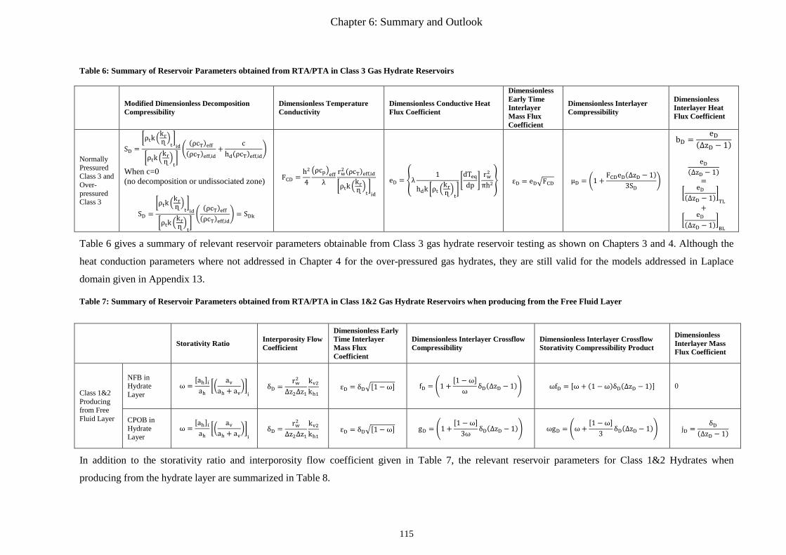
Chapter 6: Summary and Outlook
Table 6: Summary of Reservoir Parameters obtained from RTA/PTA in Class 3 Gas Hydrate Reservoirs
Modified Dimensionless Decomposition Compressibility
Dimensionless Temperature Conductivity
Dimensionless Conductive Heat Flux Coefficient
Dimensionless Early Time Interlayer Mass Flux Coefficient
Dimensionless Interlayer Compressibility
Dimensionless Interlayer Heat Flux Coefficient
Normally Pressured Class 3 and Over-pressured Class 3
SD =�ρtk �
krɳ �t
�id
�ρtk �krɳ �t
��
(ρcT)eff(ρcT)eff,id
+c
hd(ρcT)eff,id�
When c=0 (no decomposition or undissociated zone)
SD =�ρtk �
krɳ �t
�id
�ρtk �krɳ �t
��
(ρcT)eff(ρcT)eff,id
� = SDk
FCD =h2
4�ρcp�eff
λrw2 (ρcT)eff,id
�ρtk �krɳ �t
�id
eD = �λ1
hdk �ρt �krɳ �t
��dTeqdp �
rw2
πh2� εD = eD�FCD µD = �1 +
FCDeD(∆zD − 1)3SD
�
bD =eD
(∆zD − 1)
eD
(∆zD − 1)
= �
eD(∆zD − 1)�TL
+ �
eD(∆zD − 1)�BL
Table 6 gives a summary of relevant reservoir parameters obtainable from Class 3 gas hydrate reservoir testing as shown on Chapters 3 and 4. Although the
heat conduction parameters where not addressed in Chapter 4 for the over-pressured gas hydrates, they are still valid for the models addressed in Laplace
domain given in Appendix 13.
Table 7: Summary of Reservoir Parameters obtained from RTA/PTA in Class 1&2 Gas Hydrate Reservoirs when producing from the Free Fluid Layer
In addition to the storativity ratio and interporosity flow coefficient given in Table 7, the relevant reservoir parameters for Class 1&2 Hydrates when
producing from the hydrate layer are summarized in Table 8.
Storativity Ratio Interporosity Flow Coefficient
Dimensionless Early Time Interlayer Mass Flux Coefficient
Dimensionless Interlayer Crossflow Compressibility
Dimensionless Interlayer Crossflow Storativity Compressibility Product
Dimensionless Interlayer Mass Flux Coefficient
Class 1&2 Producing from Free Fluid Layer
NFB in Hydrate Layer
ω =[ah]𝑖𝑖
ah��
avah + av
��i δD =
rw2
∆z2∆z1kv2kh1
εD = δD�[1−ω] fD = �1 +[1 −ω]ω
δD(∆zD − 1)� ωfD = [ω + (1 −ω)δD(∆zD − 1)] 0
CPOB in Hydrate Layer
ω =[ah]𝑖𝑖
ah��
avah + av
��i δD =
rw2
∆z2∆z1kv2kh1
εD = δD�[1−ω] gD = �1 +[1 −ω]3ω
δD(∆zD − 1)� ωgD = �ω+[1 −ω]
3δD(∆zD − 1)� jD =
δD(∆zD − 1)
115
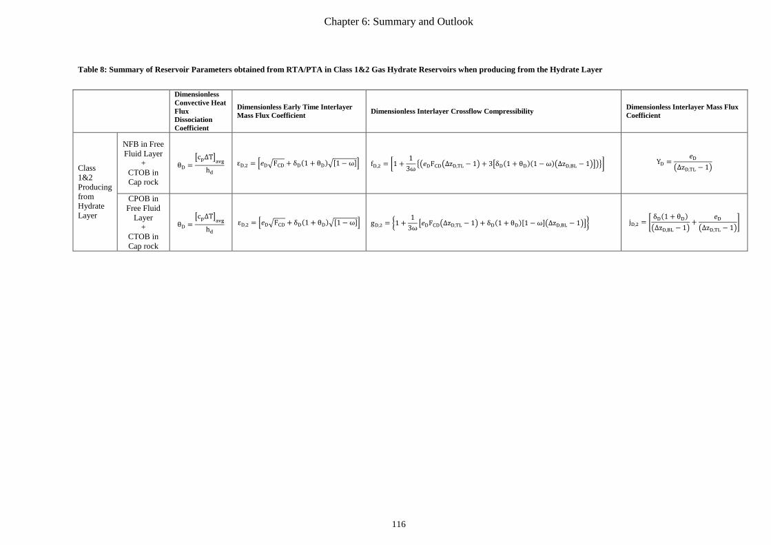
Chapter 6: Summary and Outlook
Table 8: Summary of Reservoir Parameters obtained from RTA/PTA in Class 1&2 Gas Hydrate Reservoirs when producing from the Hydrate Layer
Dimensionless Convective Heat Flux Dissociation Coefficient
Dimensionless Early Time Interlayer Mass Flux Coefficient Dimensionless Interlayer Crossflow Compressibility Dimensionless Interlayer Mass Flux
Coefficient
Class 1&2 Producing from Hydrate Layer
NFB in Free Fluid Layer
+ CTOB in Cap rock
θD =�cp∆T�
avg
hd εD,2 = �𝑉𝑉D�FCD + δD(1 + θD)�[1−ω]� fD,2 = �1 +
13ω
��𝑉𝑉DFCD�∆zD,TL − 1�+ 3�δD(1 + θD)(1−ω)�∆zD,BL − 1����� YD =𝑉𝑉D
�∆zD,TL − 1�
CPOB in Free Fluid
Layer +
CTOB in Cap rock
θD =�cp∆T�
avg
hd εD,2 = �𝑉𝑉D�FCD + δD(1 + θD)�[1−ω]� gD,2 = �1 +
13ω�
𝑉𝑉DFCD�∆zD,TL − 1�+ δD(1 + θD)[1−ω]�∆zD,BL − 1��� jD,2 = �δD(1 + θD)�∆zD,BL − 1�
+𝑉𝑉D
�∆zD,TL − 1��
116
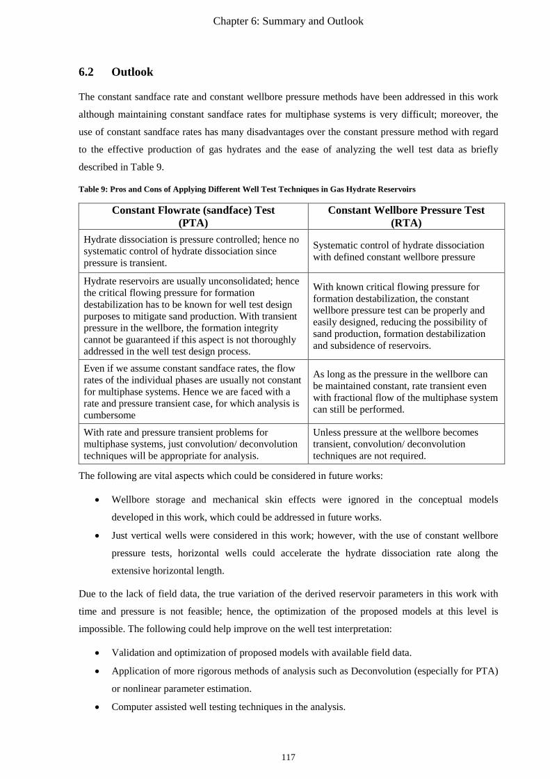
Chapter 6: Summary and Outlook
6.2 Outlook
The constant sandface rate and constant wellbore pressure methods have been addressed in this work
although maintaining constant sandface rates for multiphase systems is very difficult; moreover, the
use of constant sandface rates has many disadvantages over the constant pressure method with regard
to the effective production of gas hydrates and the ease of analyzing the well test data as briefly
described in Table 9.
Table 9: Pros and Cons of Applying Different Well Test Techniques in Gas Hydrate Reservoirs
Constant Flowrate (sandface) Test (PTA)
Constant Wellbore Pressure Test (RTA)
Hydrate dissociation is pressure controlled; hence no systematic control of hydrate dissociation since pressure is transient.
Systematic control of hydrate dissociation with defined constant wellbore pressure
Hydrate reservoirs are usually unconsolidated; hence the critical flowing pressure for formation destabilization has to be known for well test design purposes to mitigate sand production. With transient pressure in the wellbore, the formation integrity cannot be guaranteed if this aspect is not thoroughly addressed in the well test design process.
With known critical flowing pressure for formation destabilization, the constant wellbore pressure test can be properly and easily designed, reducing the possibility of sand production, formation destabilization and subsidence of reservoirs.
Even if we assume constant sandface rates, the flow rates of the individual phases are usually not constant for multiphase systems. Hence we are faced with a rate and pressure transient case, for which analysis is cumbersome
As long as the pressure in the wellbore can be maintained constant, rate transient even with fractional flow of the multiphase system can still be performed.
With rate and pressure transient problems for multiphase systems, just convolution/ deconvolution techniques will be appropriate for analysis.
Unless pressure at the wellbore becomes transient, convolution/ deconvolution techniques are not required.
The following are vital aspects which could be considered in future works:
• Wellbore storage and mechanical skin effects were ignored in the conceptual models
developed in this work, which could be addressed in future works.
• Just vertical wells were considered in this work; however, with the use of constant wellbore
pressure tests, horizontal wells could accelerate the hydrate dissociation rate along the
extensive horizontal length.
Due to the lack of field data, the true variation of the derived reservoir parameters in this work with
time and pressure is not feasible; hence, the optimization of the proposed models at this level is
impossible. The following could help improve on the well test interpretation:
• Validation and optimization of proposed models with available field data.
• Application of more rigorous methods of analysis such as Deconvolution (especially for PTA)
or nonlinear parameter estimation.
• Computer assisted well testing techniques in the analysis.
117
References
7 References
[1] M. Kome, M. Amro and Y. Cinar, „SPE-165975-MS: Analytical Models for Well Test Analysis in Class 3 Gas Hydrate Reservoirs,“ Abu Dhabi, UAE, 2013.
[2] E. Pinero, M. Marquardt, C. Hensen, M. Haeckel and K. Wallmann, „Estimation of the global inventory of methane hydrates in marine sediments using transfer functions,“ Biogeosciences 10, pg 959-975, 2013.
[3] K. C. Hester and P. G. Brewer, „Clathrate Hydrates in Nature,“ Annual Review of Marine Science, pg 303-307, 2009.
[4] http://www.futurist.com, „http://www.futurist.com,“ 17 06 2014. [Online]. Available: http://www.futurist.com/articles-archive/energy-the-future-and-us/. [Accessed on17 06 2014].
[5] J. Carroll, Natural Gas Hydrates: A Guide for Engineers, USA: Elsevier, 2009.
[6] J. E. Dendy Sloan, Clathrate of Hydrates of Natural Gases, USA: Marcel Dekker Inc., 1990.
[7] C. Ruppel, „Methane Hydrates and the Future of Natural Gas,“ USGS, USA, 2011.
[8] K. A. Kvenvolden, „Gas Hydrates- Geological Perspectives and Global Change,“ Reviews of Geophysics 31, pg. 173-187, 1993.
[9] M. D. Max, Natural Gas Hydrates in Oceanic and Permafrost Environment, Netherlands: Kluwer Academeic Publisher, 2000.
[10] S. Germai and M. Pooladi-Darvish, „An Early Time Model for Drawdown Testing of a Hydrate-Capped Gas Reservoir,“ SPE Reservoir Evaluationand Engieering, pg 595-609, 2009.
[11] T. C. Collett and G. D. Ginsburg, „Gas Hydrates in the Messoyakha Gas Field of the West Siberian Basin: A Re-Examination of the Geologic Evidence,“ International Journal of Offshore and Polar Engineering Vol.8, No.1, pg 22-29, 1998.
[12] R. Birchwood, J. Dai, D. Shelander, R. Boswell, T. Collett, A. Cook, S. Dallimore, K. Fujii, Y. Imasato, M. Fukuhara, K. Kusaka, D. Murray and T. Saeki, „Developments in Gas Hydrates,“ Oilfield Review 22, no. 1, pg 18-33, 2010.
[13] Y. F. Makogon, Hydrates of Hydrocarbons, USA: PennWell Publishing Company, 1997.
[14] Y. Ye and C. Liu, Natural Gas Hydrates:Experimental Techniques and Their Applications, Germany : Springer , 2013.
[15] http://www.giss.nasa.gov, „http://www.giss.nasa.gov/research/features/200409_methane/,“ NASA, 19 06 2014. [Online]. Available: http://www.giss.nasa.gov/research/features/200409_methane/. [Accessed on19 06 2014].
[16] F. J. Kuckuck, M. Onur and F. Hollaender, Pressure Transient Formation and Well Testing, Great Britain: Elsevier, 2010.
[17] Schlumberger, Fundamentals of Formation Testing, Texas, USA: Schlumberger Marketing Communications, 2006.
[18] S. Cantini, D. Baldini, E. Beretta, D. Loi and S. Mazzoni, „SPE 164924: Reservoir Permeability
118
References
from Wireline Formation Testers,“ SPE, London, UK, 2013.
[19] L. Ostrowski, „SPE 100234: Revival of Openhole DST: Compromising Between Wireline-Formation Testing and Cased-Hole DST,“ SPE/EAGE, Vienna, Austria, 2006.
[20] S. Ramaswami, M. Hows, D. Frese and H. Elshahawi, „SPE 164733: Pressure Transient Data from Wireline Formation Testers: When and How to use it?,“ SPE, Cairo, Egypt, 2013.
[21] A. C. Gringarten, „From Straight Lines to Deconvolution: The Evolution of the State of the Art in Well Test Analysis,“ SPE Reservoir Evaluation and Engineering, pg. 41-62, pp. 41-62, February 2008.
[22] J. A. P. D. Bourdet, „Use of Pressure Derivative in Well-Test Interpretation,“ SPE Formation Evaluation, 1989.
[23] T. v. Schroeter, F. Hollaender and A. C. Gringarten, „SPE 71574:Deconvolution of Well Test Data as a Nonlinear Total Least Squares Problem,“ SPE, New Orleans, Louisiana, USA, 2001.
[24] H. Zhuang, Dynamic Well Testing in Petroleum Exploration and Development, USA: Elsevier, 2013.
[25] M. J. Bourgeois and R. N. Horne, „Well-Test-Model Recognition With Laplace Space,“ SPE Formation Evaluation, pg. 17-25, 1993.
[26] T. v. Schroeter, F. Hollaender and A. C. Gringarten, „SPE 77688: Analysis of Well Test Data From Permanent Downhole Gauges by Deconvolution,“ SPE, San Antonio, Texas, USA, 2002.
[27] M. M. Levitan, „Practical Application of Pressure-Rate Deconvolution to Analysis of Real Well Tests,“ SPE Reservoir Evaluation & Engineering, Bde. %1 von %2http://dx.doi.org/10.2118/84290-PA, 2005.
[28] A. Dastan, „PhD Thesis:"A New Look At Nonlinear Regression In Well Testing",“ USA, 2010.
[29] G. Moridis and M. Kowalsky, „Depressurization-induced gas pdroduction from Class 1 and Class2 hydrate deposits,“ 2006.
[30] M. Kome and M. AMro, „Welltest-Konzepte für Gashydratlagerstätten (Poster and Manuscript),“ DGMK/ÖGEW Frühjahrestagung, Fachbereich Aufsuchung und Gewinnung, Celle, Deutschland, 2014.
[31] H. Kim, P. Bishnoi, R. Heidemann and S. Rizvi, „Kinetics of Methane Hydrate Decomposition,“ Chemical Engineering Science 42, pg 1645-1653, 1987.
[32] R. Al-Hussainy, „Application of Real Gas Flow Theory to Well Testing and Deliverability Forecasting,“ JPT, pg 637-642, 1965.
[33] R. G. Agarwal, „SPE 8279: Real Gas Pseudo-Time,“ SPE, 1979.
[34] H. Fujita, „The Exact Pattern of a Concentration-Dependent Diffusion in a smei-infinite Mdeium, Part 2,“ Textile Research Journal, pg 823-827, 1952.
[35] H. Fujita, „The Exact Pattern of a Concentration-Dependent Diffusion in a smei-infinite Mdeium, Part 3,“ Textile Research Journal, pg 234-240, 1954.
[36] J. Philip, „General Method of Exact Solution of the Concentration-Dependent Equation,“ CSIRO,
119
References
1959.
[37] J. Knight and J. Philips, „Exact solutions in nonlinear diffusion,“ Journal of Engineering Mathematics, pg 219-227, 1974.
[38] J. Crank, The Mathematics of Diffusion, Great Britain: Oxford University Press, 1975.
[39] K. Singh and C. Whitson, „Gas-Condensate Pseudo-pressure in Layered Reservoirs,“ SPE Reservoir Evaluation and Engineering, pg 203-213, 2010.
[40] C. W. Ø. Fevang, „Modeling Gas-Condensate Well Deliverability,“ SPE Reservoir Engineering, pg 221-230, 1996.
[41] J. Ferris, D. Knowles, R.H.Brwon and R.W.Stallman, Theory of Aquifer Tests, USA: UNITED STATES GOVERNMENT PRINTING OFFICE, 1962.
[42] H. J. R. J. P. B. C. R. Al-Hussainy, „The Flow of Real Gases Through Porous Media,“ JPT, pg 624-636, 1966.
[43] H. Fujita, „The Exact Pattern of a Concentration-Dependent Diffusion in a smei-infinite Mdeium, Part 1,“ Textile Research Journal, pg 757-760, 1952.
[44] L.Matter and D. Anderson., „An improved Pseudo-Time for Gas Reservoirs with Significant Transient Flow,“ JCPT, pg 49-54, 2007.
[45] M. Kome and M. Amro, „SPE 167682-MS: The Impact of Multiphase Flow on Well Testing Models in Gas Hydrate Reservoirs without Crossflow,“ Vienna, Austria, 2014.
[46] O. Fevang and C. H. Whitson, „Modeling Gas-Condensate Well Deliverability,“ SPE Reservoir Engineering 1996, pg 221-230, 1996.
[47] J. Jones, D. Vo and R. Raghavan, „Interpretation of Pressure-Buiildup Responses in Gas-Condensate Wells,“ SPE Formation Evaluation, pg 93-104, 1989.
[48] D. Bourdet, Well Test Analysis: The Use of Advanced Interpretation Models, Elsevier, 2002.
[49] G. Stewart, Well Test Design and Analysis, USA: PennWell Corporation , 2011.
[50] A. Boe, S. M. Skjaeveland and C. Whitson, „Two-Phase Pressure Tests Analysis,“ SPE Formation Evaluation, Vol. 4, pg. 604-610, 1989.
[51] R. L. Perrine, „Analysis of Pressure-buildup Curves,“ Drilling and Production Practice, API, pg. 482-509, 1956.
[52] K. Aziz and A. Settari, „Petroleum Reservoir Simulation,“ Applied Science Publishers Ltd, England, 1979.
[53] M. Uddin, J. W. S. Dallimore and D. Coombe, „Gas hydrate production from the Mallik reservoir: numerical history matching and long-term production forecasting,“ Geological Survey of Canada, Bulletin 601, Canada, 2012.
[54] D. Tiab and E. C. Donaldson, Petrophysics: Theory and Practice of Measuring Reservoir Rock and Fluid Transport Properties, USA: Elsevier, 2004.
[55] Y. Masuda, Y. Konno, C. L. Sheu, H. Oyama, H. Ouchi and M. Kurihara, „Relative Permeability
120
References
Curves during Hydrate Dissociation in Depressurization,“ Proceedings of the 6th International Conference on Gas Hydrates (ICGH 2008),, Canada, 2008.
[56] H. L. Stone, „Probability Model for Estimating Three-Phase Relative Permeability,“ JPT , pg 214-218, 1970.
[57] G. Moridis and M. Kowalsky, „Comparison of kinetic and equilibrium reaction models in simulating gas hydrate behaivior in porous media,“ Energy Conversion and Management 48, pg 1850-1863, 2007.
[58] A. F. V. Everdingen and W. Hurst, „The Application of the Laplace Transformation to Flow Problems in Reservoirs,“ Petroleum Transactions, AIME, pg 305-324, 1949.
[59] A. Vandenberg, „Type Curves for Analysis of Pump Tests in Leaky Strip,“ Journal of Hydrology 33, pg 15-26, 1977.
[60] M. Kamal and Y. Pan, „SPE 141572: Pressure Transient Testing Under Multiphase Flow Conditions,“ SPE, 2011.
[61] M. J. Edwardson, H. M. Girner, H. R. Parkinson, C. D. Williams and C. S. Matthews, „Calculation of Formation Temperature Disturbances Caused by Mud Circulation,“ SPE Journal of Petroleum Technology , pp. 416-426, April 1962.
[62] B. F. Towler, Fundamental Principles of Reservoir Engineering, USA: SPE Inc., 2002.
[63] F. Haefner, H. Voigt, H. Bamberg and M. Lauterbach, Geohydrodynamische Erkundgung von Erdöl-, Erdgas- und Grundwasserlagerstätten, Berlin: Zentrales Geologisches Institut, 1985.
[64] R. P. Chapius, „Assessment of Methods and Conditions to Locate Boundaries:One or Two Straight Impervious Boundaries,“ Groundwater, Volume 32, Issue 4, pg 576–582, 1994.
[65] V. Batu, Aquifer Hydraulics : A comrehensive guide to hydrogeologic data analysis, Canada: John WIley and Sons Inc., 1998.
[66] G. Ahmadi, C. Ji and D. H. SMith, „Natural gas production from gas hydrate decomposition by depressurization,“ Chemical Engineering Science 56, pg 5801-5814, 2001.
[67] G. Ahmadi, C. Ji and D. H. Smith, „Natural gas production from hydrate dissociation: An axisymmetric model,“ Journal of Petroleum Science Engineering, pg. 245-258, 2007.
[68] N. N. Verigin, I. L. Khabibullin and G. A. Khalikov, „Linear Problem of the Dissociation of the Hydrates of Gas in a Porous Medium,“ Plenum Publishing Corporation, 1980.
[69] G. Ahmadi, C. Ji and D. H. Smith, „Production of Natural Gas from Methane Hydrate by Constant Downhole Pressure Well,“ Elsevier: Energy Conversion and Mangement 48, pp. 2053-2068, 2007.
[70] M. Hantush, B. Becken, F. Burt, S. H. Jr. and A. E. Scheidegger, Advances in Hydrosciences: Hydraulics of Wells, USA: Academic Press Inc, 1964.
[71] F. Haefner, D. Sames and H. Voigt, Wärme und Stofftransport, Springer, 1992.
[72] G. Moridis, M. B. Kowalsky and K. Pruess, TOUGH+HYDRATE v1.0 Manual, 2008.
[73] M. N. Özisik, Heat Conduction, USA: John wiley and Sons Inc, 1993.
121
References
[74] H. S. Carslaw and J. C. Jaeger, Conduction of Heat in Solids, UK: Oxford University Press, 1959.
[75] A. Tarek, Reservoir Engineering Handbook, USA: Gulf Professional Publishing, 2006.
[76] B. P. Ramagost and F. F. Farshad, „SPE-10125-MS: P/Z Abnormally Pressured Gas Reservoirs,“ SPE, Texas, USA, 1981.
[77] A. C. Gringarten and H. J. R. Jr., „The Use of Source and Green´s Functions in Solving Unsteady-Flow Problems in Reservoirs,“ SPEJ Vol. 13 , pg 285 - 296, 1973.
[78] M. Abramowitz and I. Stegun, Handbook of Mathematical Functions with Formulas, Graphs, and Mathematical Tables, USA: Dover Publications, 1964.
[79] M. Kuo, W. Wang, D. Lin and C. Chiang, „An Image‐Well Method for Predicting Drawdown Distribution in Aquifers with Irregularly Shaped Boundaries,“ Ground Water, Vol 32, No.5, pp. pg 794-804, September 1994.
[80] P. Renard, „Approximate Discharge for Constant Head Test with Recharging Boundary,“ Ground Water Vol 43, pp. 439-442, June 2005.
[81] A. U. Chaudhry, Gas Well Testing Handbook, USA: Elsevier, 2003.
[82] T. Engler and D. Tiab, „Analysis of pressure and pressure derivative without type curve matching, 4 Naturally fractured reservoirs,“ Elsevier:Journal of Petroleum Science and Engineering, Nr. 15, pg 127-138, 1996.
[83] F.-. H. Escobar, J. A. Sánchez and J. H. Cantillo, „Rate Transient Analysis for Homogeneous and Hetergeneous Gas Reservoirs Using the TDS Technique,“ CT&F - Ciencia, Tecnología y Futuro, Bd. Vol 3, Nr. 4, pg 45-59, 2008.
[84] F.-H. Escobar and M. Montealegre-M., „Application of TDS Technique to Multiphase Flow,“ CT&F - Ciencia, Tecnología y Futuro, Bd. Vol 3, Nr. 4, pg 94-105, 2008.
[85] D. Tiab, „Analysis of pressure and pressure derivative without type-curve matching - Skin and Wellbore Storage,“ Elsevier: Journal of Petroleum Science and Engineering, Nr. 12, pg 171-181, 1995.
[86] D. Tiab, „Analysis of pressure and pressure derivative without type-curve matching : Vertically fractured wells in closed systems,“ Elsevier: Journal of Petroleum Science and Engineering, Nr. 11, pg 323-333, 1994.
[87] J. Warren and P. Root, „The Behavior of Naturally Fractured Reservoirs,“ SPEJ, pg 245-255, 1963.
[88] M. A. Chaudhry and S. Zubair, „Generalized Incomplete Gamma Function with Applications,“ Journal of Computational and Applied Mathematics 55, pg 99-124, 1994.
[89] J. B. R. Lee John, Pressure Transient Testing, USA: SPE Inc., 2003.
[90] J. Lee and R. A. Wattenberg, Gas Reservoir Engineering, USA: SPE Inc., 1996.
[91] C. A. Ehlig-Economides, „Dissertation: Well Test Analysis for Wells Produced at a Constant Pressure,“ California, USA, 1979.
122

References
[92] B. Buffet and D. Acher, „Global inventory of methane clathrate: sensitivity to changes in the deep ocean,“ Elsevier: Earth and Planetary Science Letters 227, pg 185-199, 2004.
123
References
8 Publications
1. Kome, M.; Amro, M,: “ Challenges in Gas Hydrate Reservoir Testing and Analysis“, SPE
Reservoir Testing: Key Enabler for Accurate Reservoir Characterisation (Poster) Dubai,
United Arab Emirates, 26–27 May 2014
2. Kome, M.; Amro, M,: “ Welltest-Konzepte für Gashydratlagerstätten“, DGMK/ÖGEW-
Frühjahrestagung 2014 (Poster Präsentation and Manuscript), Fachbereich Aufsuchung und
Gewinnung, Celle, 24./25.April 2014
3. Kome, M.; Amro, M: SPE 167682-MS “The Impact of Multiphase Flow on Well Testing
Models in Gas Hydrate Reservoirs without Crossflow” , SPE, Wien, 2014
4. Kome, M.; Amro, M.; Cinar, Y.: SPE-165975-MS “Analytical Models for Well Test Analysis
in Class 3 Gas Hydrate Reservoirs” , SPE ,Abu Dhabi, 2013
5. Kome, M.; Amro, M.; Rehmer, K.-P.: “Untersuchung und Berechnung zur Berücksichtigung
von Buckling in Tubing und Komplettierung“, DGMK/ÖGEW-Frühjahrestagung 2013,
Fachbereich Aufsuchung und Gewinnung, Celle, 18./19.April 2013.
6. Kome, M.; Amro,M.; Hossain, M. M.: A new practical approach to evaluate near wellbore
formation damage parameters based on well test analysis for gas reservoir, SPE Paper 160867,
presented at the 2012 SPE Saudi Arabia Section Technical Symposium and Exhibition held in
AlKhobar, Saudi Arabia, 8–11 April 2012,
7. Kome, M.; Fang, Ch.; Amro; M.: Well testing in unconventional gas reservoirs, Presented in
the Annual German Society for Petroleum Sciences and Coal Chemistry (DGMK), 19-20
April 2012, Celle (Germany).
124
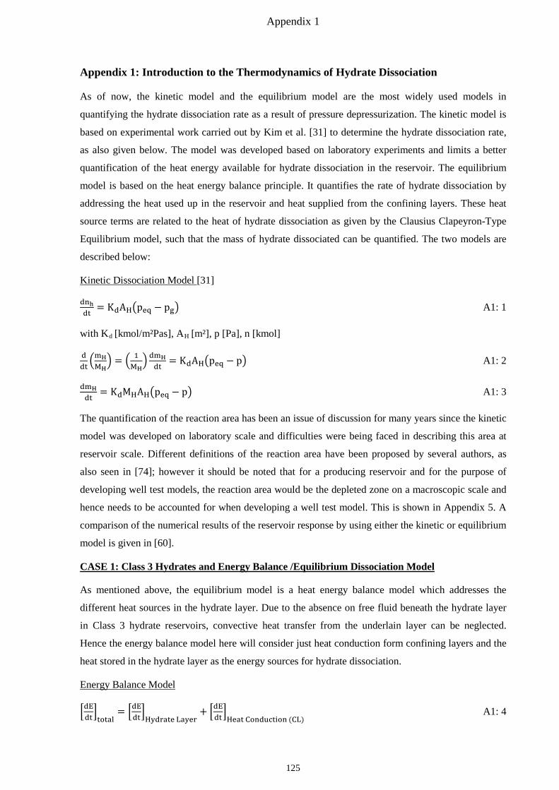
Appendix 1
Appendix 1: Introduction to the Thermodynamics of Hydrate Dissociation
As of now, the kinetic model and the equilibrium model are the most widely used models in
quantifying the hydrate dissociation rate as a result of pressure depressurization. The kinetic model is
based on experimental work carried out by Kim et al. [31] to determine the hydrate dissociation rate,
as also given below. The model was developed based on laboratory experiments and limits a better
quantification of the heat energy available for hydrate dissociation in the reservoir. The equilibrium
model is based on the heat energy balance principle. It quantifies the rate of hydrate dissociation by
addressing the heat used up in the reservoir and heat supplied from the confining layers. These heat
source terms are related to the heat of hydrate dissociation as given by the Clausius Clapeyron-Type
Equilibrium model, such that the mass of hydrate dissociated can be quantified. The two models are
described below:
Kinetic Dissociation Model [31]
dnhdt
= KdAH�peq − pg� A1: 1
with Kd [kmol/m²Pas], AH [m²], p [Pa], n [kmol]
ddt�mHMH� = � 1
MH� dmH
dt= KdAH�peq − p� A1: 2
dmHdt
= KdMHAH�peq − p� A1: 3
The quantification of the reaction area has been an issue of discussion for many years since the kinetic
model was developed on laboratory scale and difficulties were being faced in describing this area at
reservoir scale. Different definitions of the reaction area have been proposed by several authors, as
also seen in [74]; however it should be noted that for a producing reservoir and for the purpose of
developing well test models, the reaction area would be the depleted zone on a macroscopic scale and
hence needs to be accounted for when developing a well test model. This is shown in Appendix 5. A
comparison of the numerical results of the reservoir response by using either the kinetic or equilibrium
model is given in [60].
CASE 1: Class 3 Hydrates and Energy Balance /Equilibrium Dissociation Model
As mentioned above, the equilibrium model is a heat energy balance model which addresses the
different heat sources in the hydrate layer. Due to the absence on free fluid beneath the hydrate layer
in Class 3 hydrate reservoirs, convective heat transfer from the underlain layer can be neglected.
Hence the energy balance model here will consider just heat conduction form confining layers and the
heat stored in the hydrate layer as the energy sources for hydrate dissociation.
Energy Balance Model
�dEdt�total
= �dEdt�Hydrate Layer
+ �dEdt�Heat Conduction (CL)
A1: 4
125

Appendix 1
Part 1: Stored Energy in the Hydrate Layer consumed during Dissociation
In addressing the rate of heat change stored in the reservoir, the total heat energy available in the
hydrate reservoir needs to be quantified and is given by [73], [75] and [76]:
EHydrate Layer = mcpT A1: 5
The rate of change of the energy with time can hence be quantified and related to the rate of consumed
energy due to hydrate dissociation.
�dEdt�Hydrate Layer
= d(mHhd)dt
= −d�mcpT�dt
A1: 6
Differentiating the first term on the RHS of the above equation leads to:
d�mcpT�dt
= d�mcpT�dp
dpdt
= �cpT d(m)dp
+ m d�cpT�dp
� dpdt
A1: 7
Note that for pure heat conduction problems in reservoirs, the warm fluid flux is zero as there is no
mass change with pressure or time. As seen with diffusivity equations for well testing, the mass
change with pressure basically reflects the storativity of the formation which can also be related to the
pressure conductivity of the reservoir. With this said, we can conclude that the warm fluid flux and
hydrate dissociation can be well represented in the diffusivity equation.
The next step involves handling the phases separately and combining since it involves an energy
balanced system.
Gas Phase
d�mgcp,gT�dt
= �cp,gT d�V∅Sgρg�dp
+ �V∅Sgρg�d�cp,gT�
dp� dpdt
A1: 8
By assuming negligible changes in the heat capacity with pressure, the differential of the above
equation takes the form:
d�mgcp,gT�dt
= cp,gV∅Sgρg �T�cg + cF� + �dTeqdp
�� dpdt
A1: 9
Water Phase
d�mwcp,wT�dt
= cp,wV∅Swρw �T(cw + cF) + �dTeqdp
�� dpdt
A1: 10
Hydrate Phase
d�mHcp,HT�dt
= cp,HV∅SHρH �T(cF) + �dTeqdp
�� dpdt
A1: 11
Formation (Matrix)
d�mmcp,mT�dt
= �cp,FT d(Vm)dp
+ (Vm) d�cp,mT�dp
� dpdt
A1: 12
126
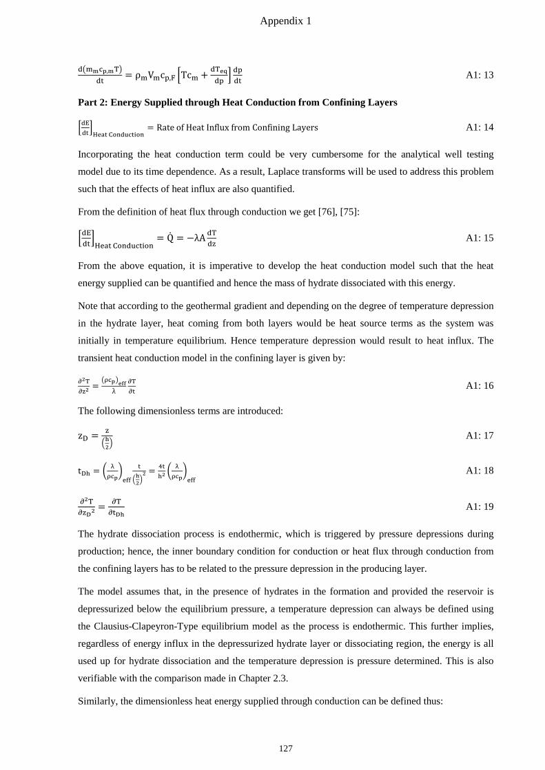
Appendix 1
d�mmcp,mT�dt
= ρmVmcp,F �Tcm + dTeqdp
� dpdt
A1: 13
Part 2: Energy Supplied through Heat Conduction from Confining Layers
�dEdt�Heat Conduction
= Rate of Heat Influx from Confining Layers A1: 14
Incorporating the heat conduction term could be very cumbersome for the analytical well testing
model due to its time dependence. As a result, Laplace transforms will be used to address this problem
such that the effects of heat influx are also quantified.
From the definition of heat flux through conduction we get [76], [75]:
�dEdt�Heat Conduction
= Q = −λA dTdz
A1: 15
From the above equation, it is imperative to develop the heat conduction model such that the heat
energy supplied can be quantified and hence the mass of hydrate dissociated with this energy.
Note that according to the geothermal gradient and depending on the degree of temperature depression
in the hydrate layer, heat coming from both layers would be heat source terms as the system was
initially in temperature equilibrium. Hence temperature depression would result to heat influx. The
transient heat conduction model in the confining layer is given by:
∂2T∂z2
=�ρcp�eff
λ∂T∂t
A1: 16
The following dimensionless terms are introduced:
zD = z
�h2� A1: 17
tDh = � λρcp�eff
t
�h2�2 = 4t
h2� λρcp�eff
A1: 18
∂2T∂zD2
= ∂T∂tDh
A1: 19
The hydrate dissociation process is endothermic, which is triggered by pressure depressions during
production; hence, the inner boundary condition for conduction or heat flux through conduction from
the confining layers has to be related to the pressure depression in the producing layer.
The model assumes that, in the presence of hydrates in the formation and provided the reservoir is
depressurized below the equilibrium pressure, a temperature depression can always be defined using
the Clausius-Clapeyron-Type equilibrium model as the process is endothermic. This further implies,
regardless of energy influx in the depressurized hydrate layer or dissociating region, the energy is all
used up for hydrate dissociation and the temperature depression is pressure determined. This is also
verifiable with the comparison made in Chapter 2.3.
Similarly, the dimensionless heat energy supplied through conduction can be defined thus:
127
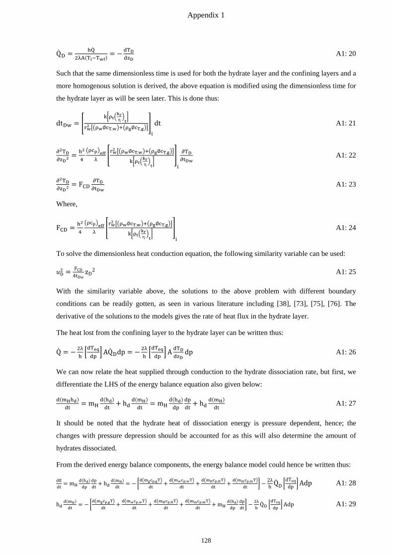
Appendix 1
QD = hQ2λA(Ti−Twf)
= −dTDdzD
A1: 20
Such that the same dimensionless time is used for both the hydrate layer and the confining layers and a
more homogenous solution is derived, the above equation is modified using the dimensionless time for
the hydrate layer as will be seen later. This is done thus:
dtDw = �k�ρt�
krɳ �t
�
rw2 ��ρw∅cT,w�+�ρg∅cT,g���i
dt A1: 21
∂2TD∂zD2
= h2
4
�ρcp�effλ
�rw2 ��ρw∅cT,w�+�ρg∅cT,g��
k�ρt�krɳ �t
��i
∂TD∂tDw
A1: 22
∂2TD∂zD2
= FCD∂TD∂tDw
A1: 23
Where,
FCD = h2
4
�ρcp�effλ
�rw2 ��ρw∅cT,w�+�ρg∅cT,g��
k�ρt�krɳ �t
��i
A1: 24
To solve the dimensionless heat conduction equation, the following similarity variable can be used:
𝑉𝑉D2 = FCD4tDw
zD2 A1: 25
With the similarity variable above, the solutions to the above problem with different boundary
conditions can be readily gotten, as seen in various literature including [38], [73], [75], [76]. The
derivative of the solutions to the models gives the rate of heat flux in the hydrate layer.
The heat lost from the confining layer to the hydrate layer can be written thus:
Q = −2λh�dTeqdp
�AQDdp = −2λh�dTeqdp
�A dTDdzD
dp A1: 26
We can now relate the heat supplied through conduction to the hydrate dissociation rate, but first, we
differentiate the LHS of the energy balance equation also given below:
d(mHhd)dt
= mHd(hd)dt
+ hdd(mH)dt
= mHd(hd)dp
dpdt
+ hdd(mH)dt
A1: 27
It should be noted that the hydrate heat of dissociation energy is pressure dependent, hence; the
changes with pressure depression should be accounted for as this will also determine the amount of
hydrates dissociated.
From the derived energy balance components, the energy balance model could hence be written thus:
dEdt
= mHd(hd)dp
dpdt
+ hdd(mH)dt
= −�d�mgcp,gT�dt
+ d�mwcp,wT�dt
+ d�mHcp,HT�dt
+ d�mmcp,mT�dt
� − 2λh QD �
dTeqdp �Adp A1: 28
hdd(mH)dt
= −�d�mgcp,gT�dt
+ d�mwcp,wT�dt
+ d�mHcp,HT�dt
+ d�mmcp,mT�dt
+ mHd(hd)dp
dpdt� − 2λ
hQD �
dTeqdp
�Adp A1: 29
128
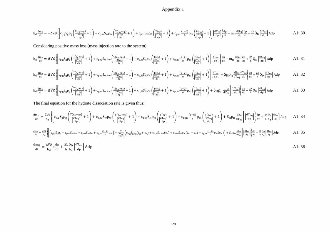
Appendix 1
hddmH
dt= −∆V∅ ��cp,gSgρg �
T�cg+cF�
�dTeqdp �
+ 1� + cp,wSwρw �T(cw+cF)
�dTeqdp �
+ 1� + cp,HSHρH �T(cF)
�dTeqdp �
+ 1� + cp,m(1−∅)∅
ρm �T(cm)
�dTeqdp �
+ 1�� �dTeqdp
�� dpdt− mH
d(hd)dp
dpdt− 2λ
hQD �
dTeqdp
�Adp A1: 30
Considering positive mass loss (mass injection rate to the system):
hddmH
dt= ∆V∅��cp,gSgρg �
T�cg+cF�
�dTeqdp �
+ 1� + cp,wSwρw �T(cw+cF)
�dTeqdp �
+ 1� + cp,HSHρH �T(cF)
�dTeqdp �
+ 1� + cp,m(1−∅)∅
ρm �T(cm)
�dTeqdp �
+ 1�� �dTeqdp
�� dpdt
+ mHd(hd)dp
dpdt
+ 2λh
QD �dTeqdp
�Adp A1: 31
hddmH
dt= ∆V∅��cp,gSgρg �
T�cg+cF�
�dTeqdp �
+ 1� + cp,wSwρw �T(cw+cF)
�dTeqdp �
+ 1� + cp,HSHρH �T(cF)
�dTeqdp �
+ 1� + cp,m(1−∅)∅
ρm �T(cm)
�dTeqdp �
+ 1�� �dTeqdp
� + SHρHdhddTeq
dTeqdp � dp
dt+ 2λ
hQD �
dTeqdp
�Adp A1: 32
hddmH
dt= ∆V∅��cp,gSgρg �
T�cg+cF�
�dTeqdp �
+ 1� + cp,wSwρw �T(cw+cF)
�dTeqdp �
+ 1� + cp,HSHρH �T(cF)
�dTeqdp �
+ 1� + cp,m(1−∅)∅
ρm �T(cm)
�dTeqdp �
+ 1� + SHρHdhddTeq
� �dTeqdp
�� dpdt
+ 2λh
QD �dTeqdp
�Adp A1: 33
The final equation for the hydrate dissociation rate is given thus:
dmHdt
= ∆V∅hd
��cp,gSgρg �T�cg+cF�
�dTeqdp �
+ 1� + cp,wSwρw �T(cw+cF)
�dTeqdp �
+ 1� + cp,HSHρH �T(cF)
�dTeqdp �
+ 1� + cp,m(1−∅)∅
ρm �T(cm)
�dTeqdp �
+ 1� + SHρHdhddTeq
� �dTeqdp
�� dpdt
+ 2λ
h
QD
hd�dTeq
dp�Adp A1: 34
dmH
dt= ∆V∅
hd���cp,gSgρg + cp,wSwρw + cp,HSHρH + cp,m
(1−∅)∅
ρm�+ T
�dTeqdp �
�cp,gSgρg�cg + cF�+ cp,HSHρH(cF) + cp,wSwρw(cw + cF) + cp,m(1−∅)∅
ρm(cm)�+ SHρHdhddTeq
� �dTeqdp
�� dpdt
+ 2λhQDhd�dTeqdp
�Adp A1: 35
dmHdt
= ∆V∅hd
c dpdt
+ 2λhQDhd�dTeqdp
�Adp A1: 36
129
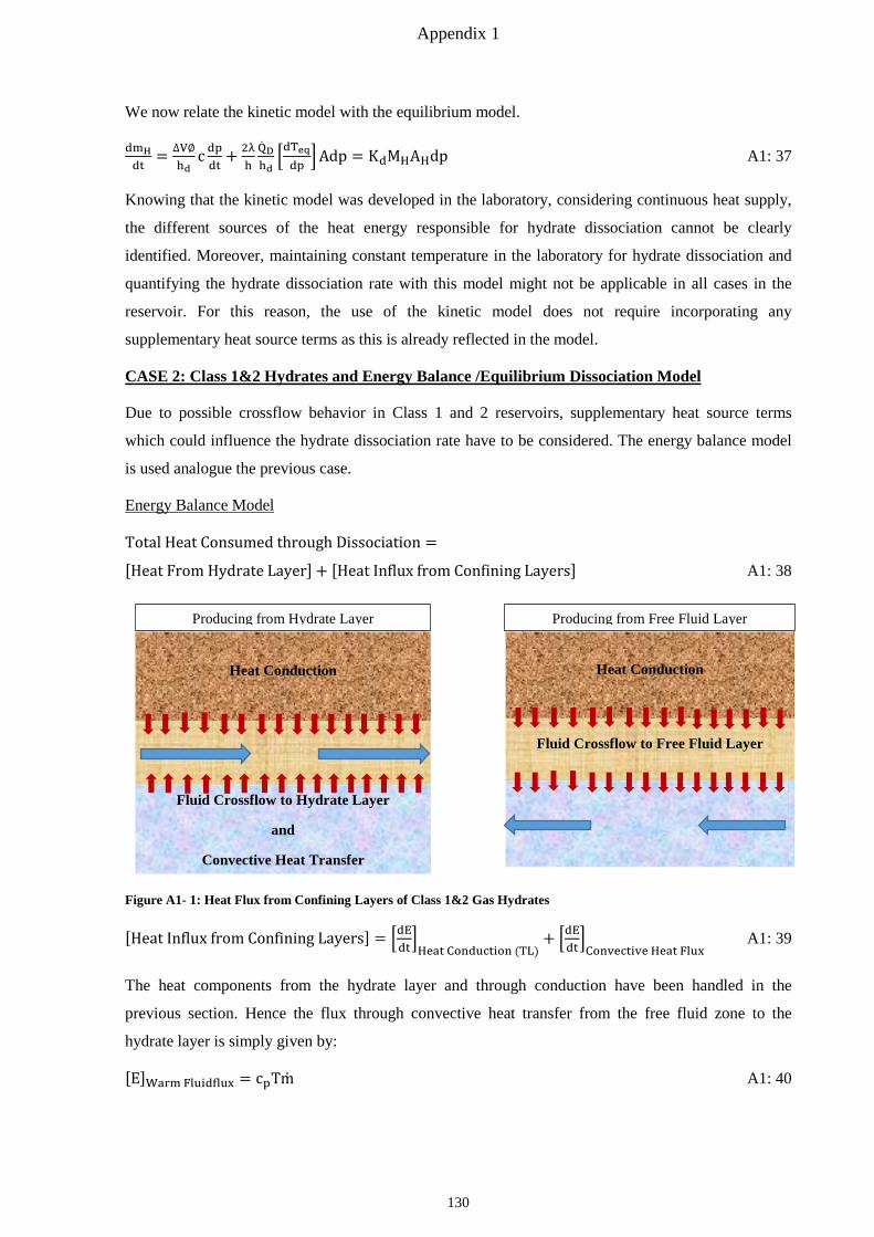
Appendix 1
We now relate the kinetic model with the equilibrium model.
dmHdt
= ∆V∅hd
c dpdt
+ 2λhQDhd�dTeqdp
�Adp = KdMHAHdp A1: 37
Knowing that the kinetic model was developed in the laboratory, considering continuous heat supply,
the different sources of the heat energy responsible for hydrate dissociation cannot be clearly
identified. Moreover, maintaining constant temperature in the laboratory for hydrate dissociation and
quantifying the hydrate dissociation rate with this model might not be applicable in all cases in the
reservoir. For this reason, the use of the kinetic model does not require incorporating any
supplementary heat source terms as this is already reflected in the model.
CASE 2: Class 1&2 Hydrates and Energy Balance /Equilibrium Dissociation Model
Due to possible crossflow behavior in Class 1 and 2 reservoirs, supplementary heat source terms
which could influence the hydrate dissociation rate have to be considered. The energy balance model
is used analogue the previous case.
Energy Balance Model
Total Heat Consumed through Dissociation =
[Heat From Hydrate Layer] + [Heat Influx from Confining Layers] A1: 38
Figure A1- 1: Heat Flux from Confining Layers of Class 1&2 Gas Hydrates
[Heat Influx from Confining Layers] = �dEdt�Heat Conduction (TL)
+ �dEdt�Convective Heat Flux
A1: 39
The heat components from the hydrate layer and through conduction have been handled in the
previous section. Hence the flux through convective heat transfer from the free fluid zone to the
hydrate layer is simply given by:
[E]Warm Fluidflux = cpTm A1: 40
Fluid Crossflow to Hydrate Layer
and
Convective Heat Transfer
Heat Conduction
Fluid Crossflow to Free Fluid Layer
Heat Conduction
Producing from Hydrate Layer Producing from Free Fluid Layer
130
Appendix 1
The representation assumes that the temperature in the free fluid zone is approximately constant
throughout the depletion period and the rate of hydrate dissociation would be a function of the
temperature difference between the hydrate layer after endothermic dissociation and the incoming
fluid. Hence the hydrate dissociation rate from the energy supplied is given by:
dmHdt
= cphd
mz∆T =�cp∆T�avg
hd� ∆x ∗ ∆y ∗ ∆(ρg ∗ wg) + ∆x ∗ ∆y ∗ ∆(ρw ∗ ww)� A1: 41
Incorporating the above model in the diffusivity equation is addressed comprehensively in Appendix
14.
Conventionally, the mass rate of each phase would have to be addressed separately and the specific
heat capacities as well. However, since the diffusivity equation developed here considers the total
mass rate, an average specific heat capacity will be assumed and the total mass leakage rate for the
crossflow layer derived.
The rate of hydrate dissociation can hence be defined thus:
dmHdt
=�cp∆T�avg
hdmz + ∆V∅
hdc dpdt
+ 2λhQDhd�dTeqdp
�Adp A1: 42
If energy and mass balance hold, the kinetic and equilibrium model should be equal; hence:
dmHdt
= KdMHAHdp =�cp∆T�avg
hdmz + ∆V∅
hdc dpdt
+ 2λhQDhd�dTeqdp
�Adp A1: 43
dmHdt
= KdMHAHdp = ∆mH,2(p, t) + mH(p) + ∆mH,1(p, t) A1: 44
This implies, instead of using the different heat energy sources, the kinetic model could be used to
investigate the rate of hydrate dissociation and hence type curves generated. Nonetheless, the effects
of the different heat source terms can be comprehensively investigated using the equilibrium model.
131
Appendix 2
Appendix 2: Equation of State (EOS) for Hydrate Dissociation
In Appendix 1, the rate of hydrate dissociation was quantified using the equilibrium model; however,
it is still essential in depicting the equivalent masses or volumes of the hydrate components generated
from the dissociation process. The amount of gas generated from the gas hydrate at standard
conditions could be estimated using the simple EOS as given below:
Methane Hydrate = CH4*5.75 H2O A2: 1
Note that water and gas in the hydrate have a non-stoichiometric bond and hence in the Methane
Hydrate above, a total of 6.75 Moles is usually assumed, as given in [5]. Though this is the case for the
hydrate, it is usually considered to be equal to a mole of hydrate [6] and the dissociation enthalpies are
given for this unit mole of Hydrate.
From mass balance principle, the total mass of the hydrate is the sum of the masses in the hydrates:
mHydrate = mCH4 + mH2O A2: 2
This could be represented in form of the moles and molar masses thus:
MHydrate(nCH4 + nH2O) = nCH4MCH4 + nH2OMH2O A2: 3
MHydrate = nCH4(nCH4+nH2O) MCH4 + nH2O
(nCH4+nH2O) MH2O A2: 4
By assuming the number of moles in the hydrate to be equal 1, which is the case in some literature [6],
the molar mass deduced equals:
MHydrate = nCH4MCH4 + nH2OMH2O = 119,61kg/kmol A2: 5
By assuming the total number of moles in the non-stoichiometric bond of hydrates to be equal to the
sum of the number of moles present, which is also the case in some literature [5] we get the following:
MMethane Hydrate = nCH4(nCH4+nH2O) MCH4 + nH2O
(nCH4+nH2O) MH2O = 17.72 kg/kmol A2: 6
This is very crucial in determining the heat of dissociation per unit mass of the hydrates as the
dissociation enthalpies are given in joules per mole hydrate, i.e. ∆H=hF[J/kg]*MHyd [kg/mol].
It should strongly be emphasized that the enthalpy of dissociation is derived for the total number of
moles present in the gas hydrate as given by the Clausius Clapeyron models. Hence caution should be
taken in deriving the heat of dissociation per unit mass hydrate which is required for the well testing
model.
Equivalent Volumes of Byproducts
The aim of these calculations is to derive the equivalent volumes of water and gas producible from the
hydrates at standard conditions after depressurization. Mass balance principle is applied for each of the
phases as given below:
132
Appendix 2
Gas Phase
From Mass Balance
mCH4 = PstVCH4,stRTst
MCH4 A2: 7
mCH4 = nCH4MCH4 = nCH4(nCH4+nH2O) ∗
mhydrate
MhydrateMCH4 = nCH4
(nCH4+nH2O) ∗Vhydrateρhydrate
MhydrateMCH4 A2: 8
Applying mass balance to the two equations above yields:
VCH4,stVhydrate
= Eg = nCH4(nCH4+nH2O) ∗
ρhydrateMhydrate
RTstPst
= 0.14815 91317.72
8.314∗288.15∗1000101325
= 180.47 A2: 9
From the formation volume factor concept we can get the equivalent volume at reservoir conditions
thus:
VCH4Vhydrate
= EgBg A2: 10
Water Phase
As was done with the gas phase, the same mass balance approach is made here:
Vw,st = nwMwρw,st
= nH2O(nCH4+nH2O) ∗ nhydrate
Mwρw,st
= nH2O(nCH4+nH2O) ∗
ρhydrateVhydrateMhydrate
Mwρw,st
A2: 11
Vw,stVhydrate
= Ew = nH2O(nCH4+nH2O) ∗
ρhydrateMhydrate
Mwρw,st
= 0.85185 91317.72
18.0151000
= 0.79 A2: 12
VwVhydrate
= EwBw A2: 13
Equivalent Masses of Byproducts
Total Gas Concentration and Gas Production Rate
mg,H
mh=
ng�ng+nw�∗
VHρHMH
Mg
ρHVH= ng
�ng+nw�∗ Mg
MH A2: 14
mg,H = � ng
�ng+nw�∗
Mg
MH� mH A2: 15
Total Water Concentration and Water Production Rate
mw,Hmh
=nw
�ng+nw�∗VHρHMH
Mw
ρHVH= nw
�ng+nw�∗ MwMH
A2: 16
mw,H = � nw
�ng+nw�∗ Mw
MH� mH A2: 17
Hydrate Dissociation Rate with Fluid Components
mH = mw,H + mg,H = �nwMw+ngMg��ng+nw�MH
mH A2: 18
133
Appendix 3
Appendix 3: Clausius Clapeyron Type Equations and the Heat of Hydrate Dissociation
In Appendix 1 and Appendix 2, the mass dissociation rate is given as a function of the hydrate
dissociation energy which must be derived from the Clausius-Clapeyron model represented thus [5]:
dTdP
= zRT2
p∆H= zRT2
phFMHyd A3: 1
∆H [J/mol] represents the enthalpy of fusion, also denoted by ∆H=hF[J/kg]*MHyd [kg/mol]; P and T
represent the reservoir pressure and temperature conditions at which the hydrate is stable.
Integrating the Clausius-Clapeyron equation results to:
lnp = − ∆HzRT
A3: 2
In order to derive the analytically the hydrate dissociation energy, a Clausius Clapeyron type phase
equilibrium model is required. For this work, the Carroll and Duan [5] prediction model will be used.
The model is given below:
lnP = A + BT + CT
+ DlnT A3: 3
Where A, B, C, D are empirical constants, also given below for methane hydrates.
Differentiating Carroll´s equation with respect to temperature results to:
d lnpdT
= B − CT²
+ DT
A3: 4
Or
d pdT
= �B − CT²
+ DT� eA+BT+
CT+DlnT A3: 5
dTeqdp
= 1
�d pdT�
= 1
��B−CT²+
DT�e
A+BT+CT+DlnT� A3: 6
From the model above, the temperature depression due to hydrate dissociation can be estimated as
given below.
Temperature Change from Hydrate Dissociation
T(p) = Teq − �dTeqdp
� �peq − p� A3: 7
The equation above suggests that depressurization is the activating mechanism for any heat influx in
the hydrate layer which will further trigger hydrate dissociation. This further implies, as long as
hydrates are depressurized, the temperature in the hydrate layer will be pressure controlled and any
heat flux in the layer will be used up for dissociation and the endothermic process continues.
134
Appendix 3
Heat of Fusion/Dissociation for Unit Mass Hydrate
Using the Clausius-Clapeyron model and Carroll´s equation, we could derive the heat of dissociation
for a given hydrate at known reservoir p, T conditions thus:
d lnpdT
= B − CT2
+ DT
= ∆HzRT2
= hFMHyd
zRT² A3: 8
From Carroll´s Equation for methane hydrate:
A= -146.1094 [-]; B=0.3165 [1/K]; C=16556.78 [K]; D=0 [-]
Method 1
The enthalpy of dissociation is usually derived per unit mole thus:
MHydrate = nCH4MCH4 + nH2OMH2O = 119,61kg/kmol
d lnpdT
= ∆H zRT2
= hFMHyd
zRT² A3: 9
Hence the heat of dissociation could be derived thus:
hF = ∆HMHyd
= hd A3: 10
Method 2
By assuming the total number of moles in the non-stoichiometric bond of hydrates to be equal to the
sum of the moles, we get:
MHyd2 = nCH4(nCH4+nH2O) MCH4 + nH2O
(nCH4+nH2O) MH2O = 17.72 kg/kmol A3: 11
The heat of dissociation should be derived thus:
hF = ∆H(nCH4+nH2O)∗MHyd2
= hd A3: 12
Change of Dissociation Enthalpy with Temperature / Pressure
As shown in Appendix 1, the changes in the hydrate dissociation energy with pressure needs to be
derived in order to better quantify the hydrate dissociation rate. This is derived thus:
∆H = (BT² − C + DT)zR A3: 13
d∆HdT
= (2BT + D)zR A3: 14
Hence the heat of dissociation could be derived thus:
dhFdp
= dhFdT
∗ dTdp
= (2BT+D)zRMHyd
∗ 1
��B−CT²+
DT�e
A+BT+CT+DlnT� A3: 15
135
Appendix 4
Appendix 4: Permeability and Saturation for Hydrate Dissociation
In the previous appendices, efforts were made to quantify the mass of gas and water generated from
the hydrate dissociation. In this section, the increase in gas and water saturation will be quantified such
that this can be incorporated into the relative permeability terms and would give a stronger support for
future reservoir simulation works and computer aided well testing approaches. This should further
give a clearer image of the influence of the different heat source terms on the dissociation rate and the
quantity of water and gas generated. Ignoring convective heat flux due to crossflow, the following
approach can be made:
Gas Phase
mg,H = � ng
�ng+nw�∗
Mg
MH� mH A4: 1
mg,H = � ng�ng+nw�
∗ Mg
MH�mH = � ng
�ng+nw�∗ Mg
MH� �V∅
hd{c} + 2λ
hQDhd�dTeqdp
�At� �peq − p� A4: 2
Sg,H(p, t) = � EgBgEgBg+EwBw
� �c + 2λhV∅
QD �dTeqdp
�At� �peq−p�hdρH
SH A4: 3
Where,
� ng�ng+nw�
∗ Mg
MH∗ρHρg,eq
� = � EgBgEgBg+EwBw
� A4: 4
Without Heat Conduction
Sg,H(p) = � EgBgEgBg+EwBw
� [c] �peq−p�hdρH
SH A4: 5
Water Phase
mw,H = � nw
�ng+nw�∗ Mw
MH� mH A4: 6
Sw,H(p) = � EwBwEgBg+EwBw
� �c + 2λhV∅
QD �dTeqdp
�At� �peq−p�hdρH
SH A4: 7
Where,
� nw�ng+nw�
∗ MwMH
∗ρHρw,eq
� = � EgBgEgBg+EwBw
� A4: 8
Without Heat Conduction
Sw,H(p) = � EwBwEgBg+EwBw
� [c] �peq−p�hdρH
SH A4: 9
Let;
c∗(p, t) = �c + 2λhV∅
QD �dTeqdp
�At� A4: 10
136
Appendix 4
Hydrate Phase
SH(p, t) = �1− [c∗] �peq−p�hdρH
� SH A4: 11
SH(p, t) = SH − [c∗] �peq−p�hdρH
SH = SH − ∆SH A4: 12
∆SH = �� EwBwEgBg+EwBw
� [c∗] �peq−p�hdρH
SH� + �� EgBgEgBg+EwBw
� [c∗] �peq−p�hdρH
SH� = [c∗] �peq−p�hdρH
SH A4: 13
∆SH = Sw,H + Sg,H A4: 14
Effective and Relative Permeability of Gas hydrate
kH = k(1 − SH)N = k ∗ krH A4: 15
kg = krgkH = �krg ∗ krH� ∗ k = krg∗ ∗ k = �Sgeff−Sgirr1−Sgirr
�ng
k A4: 16
kw = krwkH = (krw ∗ krH) ∗ k = krw∗ ∗ k = �Sweff−Swirr1−Swirr
�nw
k A4: 17
Care should be taken when computing the relative permeabilities as hydrate dissociation causes an
increase in saturation for both phases and hence conventional relative permeability curves will differ
from this.
Gas is a very compressible medium and is hence very pressure sensitive. This implies the volume of
gas or saturation is also very pressure sensitive. Pressure depletion decreases the saturation of free
fluid available and simultaneously, fluid is produced through hydrate dissociation, which increases the
saturation once more. The material balance in terms of saturation can be represented below:
Swi = 1 − Sgi − SHi A4: 18
Sw(p) + ∆Sw(p) = 1 − �Sg(p) + ∆Sg(p)� − [SH(p) + ∆SH] A4: 19
Sw(p) + ∆Sw(p) = 1 − �Sg(p) + ∆Sg(p)� − �SH(p) + Sw,H + Sg,H� A4: 20
The above equation could be rearranged such that we get the effective changes in saturation as a result
of production of each phase. The resulting equation would be:
Sw,eff = 1 − Sg,eff − SH(p) A4: 21
Where,
Sw,eff = Sw(p) + Sw,H + ∆Sg(p) A4: 22
Sg,eff = Sg(p) + Sg,H + ∆Sw(p) A4: 23
The above equations for the effective saturations depict that a reduction in saturation of one phase
increases the saturation of the other phase. Although the increase in gas and water saturations as a
137
Appendix 4
result of hydrate dissociation have been addressed earlier, the dependence of fluid saturation on
pressure has not been depicted.
Material Balance Approach for Fluid Saturation Dependence on Pressure
The dependence of the hydrate saturation on pressure has been fully discussed in the previous
appendices. It is now imperative to investigate the changes in free fluid saturation on pressure, which
is relevant for any simulation calculation and also in investigating the changes in relative permeability
during depletion.
Fluid saturation in the pores of the formation could be represented thus:
Sfl = VflVp
= VstBVp
= VstVp
ρstρfl
= Vst∅V
ρstρfl
A4: 24
In the above equation, the density of the reservoir fluids and the porosity are pressure dependent.
Hence, the derivative of the above function with pressure is given by:
dSfldp
= VstρstV
d� 1∅ρfl
�
dp A4: 25
From the above equation, it should be noted that for positive pressure depressions in the reservoir, the
saturation change is negative. To eliminate this effect, a negative sign is introduced in front of the
RHS of the above equation.
dSfldp
= −VstρstV
d� 1∅ρfl
�
dp A4: 26
dSfldp
= VstBVp
�1∅d∅dp
+ 1ρfl
dρfldp� A4: 27
∫ 1Sfl
dSfl = ∫ �1∅ d∅ + 1ρfl
dρfl� A4: 28
Sfl = Sfl,i �∅∅i∗ ρflρfl,i� A4: 29
Since the porosity and density are pressure dependent parameters, the saturation will also show
pressure dependent properties.
Gas Phase
Sg(p) = Sg,i �∅∅i∗ ρgρg,i� A4: 30
∆Sg(p) = Sg,i − Sg(p) = Sg,i �1 − �∅∅i∗ ρgρg,i�� A4: 31
Water Phase
Sw(p) = Sw,i �∅∅i∗ ρwρw,i
� A4: 32
138
Appendix 4
∆Sw(p) = Sw,i − Sw(p) = Sw,i �1 − �∅∅i∗ ρwρw,i
�� A4: 33
It can be easily shown that the above models can be used to derive volumetric material balance
method used in deriving the original gas in place from p/z-plots, which further validates the above
model proposed for the dependence of fluid saturation on pressure.
Material Balance Approach for Fluid Saturation and P/Z-Plot for Gas Reservoirs
Sfl,i Sfl,i
− Sfl(r,t)
Sfl,i = Gp(t) = �∅i
∅i∗ ρfl,iρfl,i� − �∅
∅i∗ ρflρfl,i� A4: 34
Gp(t) = ρstρfl,i∅i
��∅ipiTstpstTizi
� − �∅ pTstpstTz
�� A4: 35
Gp,st(t) = Gp(t)Bgi
= Tstpst�� piTizi
� − �∅∅i
pTz�� A4: 36
The porosity change with pressure is given by [77]:
∅∅i
= e−cf,i(pi−p) A4: 37
We write the general material balance equation thus:
� pTz
e−cf,i(pi−p)� = �� piTizi
� − pstTst
Gp,st(t)� A4: 38
For conventional gas reservoirs where the temperature is assumed constant during depletion, the above
equation is simplified thus:
pz�1 − cf,i(pi − p)� = pi
zi− pstTi
TstGp,st(t) A4: 39
pz�1 − cf,i(pi − p)� = pi
zi�1− pstTizi
TstpiGp,st(t)� A4: 40
pz�1 − cf,i(pi − p)� = pi
zi�1 − Gp,st(t)
G� A4: 41
The model has now been represented similar to the material balance model given by Ramagost and
Farshad [78] with the modification of the apparent compressibility. It should be highlighted at this
point that the effect of hydrate dissociation will lead to an increase in the amount of gas produced and
hence a deviation to the right from the normal p/z-plot which is similar to aquifer-drive reservoirs.
If the porosity change is assumed to be trivial throughout depletion, then the above equation is further
simplified to the conventional volumetric p/z-plot thus:
pz
= pizi− pstT
TstGp,st(t) A4: 42
139

Appendix 4
Material Balance Approach for Gas Hydrate Reservoirs
If the same procedure is applied to the gas hydrate reservoir and considering the multiphase system,
the following material balance model can be developed for gas hydrate reservoirs:
GpBg,i
+ WpBw,i
= V∅iSg,i ���1Bg,i� − �∅
∅i∗ 1Bg�� + 1
Bg,i
Sg,H
Sg,i� + V∅iSw,i
Bw,iBg,i
��� 1Bw,i
� − �∅∅i∗ 1Bw�� + 1
Bw,i
Sw,HSw,i
� A4: 43
140

Appendix 5
Appendix 5: Basics of Diffusivity Equations in Gas Hydrate Reservoirs
The mass balance equation for the hydrate layer is given in cylindrical coordinates thus:
2πh∆(r ∗ ρg ∗ wg) + 2πh∆(r ∗ ρw ∗ ww) = 2πrh∆r ∆�Sg∅ρg�∆t
+ 2πrh∆r ∆(Sw∅ρw)∆t
+ Source A5: 1
2πh∆(r ∗ ρg ∗ wg) + 2πh∆(r ∗ ρw ∗ ww) = 2πrh∆r ∆�Sg∅ρg�∆t
+ 2πrh∆r ∆(Sw∅ρw)∆t
+ mH A5: 2
The source term in the above mass balance equation is due to hydrate dissociation into its byproducts
and can be defined using the equilibrium model or the kinetic model as given below and also in
Appendix 1.
Kinetic Model
The kinetic model as given by [31] considers the rate of hydrate dissociation considering the available
area for reaction and the activation energy needed to initiate hydrate dissociation. It however does not
quantify the heat energy available in the reservoir and does not define the source of heat responsible
for hydrate dissociation. However, as shown in Appendix 1, the total heat supplied and the total
hydrate dissociated could be assumed to be reflected in the kinetic model, and hence the hydrate
dissociation rate can better be reflected in type curves. Incorporating the kinetic model proposed by
Kim et al. [31] into the diffusivity equation, we get:
2πh∆(r ∗ ρg ∗ wg) + 2πh∆(r ∗ ρw ∗ ww) − KdMHAH∆p = 2πrh∆r ∆�Sg∅ρg�∆t
+ 2πrh∆r ∆(Sw∅ρw)∆t
A5: 3
As mentioned in Appendix 1, the hydrate reaction area for a producing reservoir will be defined such
that it reflects the depleting zone.
∆(r∗ρg∗wg)r∆r
+ ∆( r∗ρw∗ww)r∆r
− KdMHπr∆r2πh
∆pr∆r
= ∆�Sg∅ρg�∆t
+ ∆(Sw∅ρw)∆t
A5: 4
1r
∂(r∗ρg∗wg) ∂r
+ 1r
∂(r∗ρw∗ww) ∂r
− KdMH
2h�pi − p� = (ρcT)eff
∂p∂t
A5: 5
Where,
(ρcT)eff = �Sg∅ρg�cg + cF� + Sw∅ρw[cw + cF]� A5: 6
∂(r∗ρg∗wg) ∂r
+ 1r
∂(r∗ρw∗ww) ∂r
− KdMH
2h�pi − p� = (ρcT)eff
∂p∂t
A5: 7
Considering mass balance and neglecting capillary pressure effects, the above equation takes the form:
∂�r∗�ρg∗khkrgɳg+ρw∗kh
krwɳw
�∂p∂r�
∂r− KdMH
2h(pi − p) = (ρcT)eff
∂p∂t
A5: 8
By using the pseudo-pressure model, the diffusivity equation can be written in the form:
1r
∂�r∂φ∂r�
∂r− KdMH
2hk�ρt�krɳ �t
�(φi − φ) = (ρcT)eff
∂p∂t
A5: 9
141
Appendix 5
Such that the effects of changes in the effective compressibility are accounted for in the well test
model, the following approach is made (It should be noted that other approaches such as the use of
pseudo-time could be used):
1r
∂�r∂φ∂r�
∂r− KdMH
2hk�ρt�krɳ �t
�(φi − φ) = (ρcT)eff
(ρcT)eff,id(ρcT)eff,id
∂p∂t
A5: 10
∂2φD∂rD2
+ 1rD
∂φD ∂rD
− KdMHrw2
2hkft(𝐶𝐶) φD = (ρcT)eff(ρcT)eff,id
�ρt�krɳ �t
�id
�ρt�krɳ �t
�
∂φD∂tDw
A5: 11
∂2φD∂rD2
+ 1rD
∂φD ∂rD
− γDkφD = SDk∂φD∂tDw
A5: 12
Where,
γDk = KdMHrw2
2hkft(𝐶𝐶) = Koe�−ERT�MHrw2
2hk�ρt�krɳ �t
� A5: 13
SDk =�ρt�
krɳ �t
�id
�ρt�krɳ �t
�� (ρcT)eff
(ρcT)eff,id� A5: 14
tDw =𝑘𝑘�ρt�
krɳ �t
�id
rw2(ρcT)eff,idt A5: 15
Equilibrium Model
In the equilibrium model, the source term is quantified using an energy balance approach, such that the
available energy in the reservoir and its changes are related to the energy required for hydrate
dissociation. Using the equilibrium model we get:
2πh∆(r ∗ ρg ∗ wg) + 2πh∆(r ∗ ρw ∗ ww) = 2πrh∆r ∆�Sg∅ρg�∆t
+ 2πrh∆r ∆(Sw∅ρw)∆t
+ mH A5: 16
Equilibrium Model for Class 3 Gas Hydrate Reservoir
We first derive the diffusivity equation for Class 3 gas hydrates by incorporating the hydrate
dissociation rate derived in Appendix 1 into the mass balance equation given above:
2πh∆(r ∗ ρg ∗ wg) + 2πh∆(r ∗ ρw ∗ ww) − 2λhQDhd�dTeqdp
�A(pi − p) = 2πrh∆r �∆�Sg∅ρg�∆t
+ ∆(Sw∅ρw)∆t
+ ∆(Sh∅ρh)∆t
� A5: 17
1r
∂�r∗�ρg∗kkrg∗
ɳg+ρw∗
krw∗
ɳw�∂p∂r�
∂r− λ
h2QDhd�dTeqdp
� �pi − p� = ��ρw∅cT,w�+ �ρg∅cT,g��∂p∂t
+ c
hd
∂p∂t
A5: 18
1rD
∂�rD∂φ∂rD
�
∂rD− λ
h2QDrw
2
hdk�ρt�krɳ �t
��dTeqdp
� (φi − φ) = (ρcT)effrw2
�ρtk�krɳ �t
�
∂φ∂t
+ c
hd
rw2
�ρtk�krɳ �t
�
(ρcT)eff,id(ρcT)eff,id
∂φ∂t
A5: 19
142
Appendix 5
1rD
∂�rD∂φ∂rD
�
∂rD− λ
h2QDrw
2
hdkft(𝐶𝐶) �dTeqdp
� (φi − φ) = (ρcT)effrw2
�ρtk�krɳ �t
�
∂φ∂t
+ c
hd
rw2
�ρtk�krɳ �t
�
(ρcT)eff,id(ρcT)eff,id
∂φ∂t
A5: 20
1rD
∂�rD∂φ∂rD
�
∂rD− eDQD(φi − φ) = (ρcT)effrw2
�ρtk�krɳ �t
�
∂φ∂t
+ c
hd
rw2
�ρtk�krɳ �t
�
(ρcT)eff,id(ρcT)eff,id
∂φ∂t
A5: 21
1rD
∂�rD∂φ∂rD
�
∂rD− eDQD(φi − φ) = (ρcT)eff
(ρcT)eff,id
�ρtk�krɳ �t
�id
�ρtk�krɳ �t
�
rw2(ρcT)eff,id
�ρtk�krɳ �t
�id
∂φ∂t
+ chd(ρcT)eff,id
�ρtk�krɳ �t
�id
�ρtk�krɳ �t
�
rw2(ρcT)eff,id
�ρtk�krɳ �t
�id
∂φ∂t
A5: 22
∂2φD∂rD2
+ 1rD
∂φD ∂rD
− γDeφD =�ρtk�
krɳ�
t�
id
�ρtk�krɳ�
t�� (ρcT)eff
(ρcT)eff,id+ c
hd(ρcT)eff,id� ∂φD∂tDw
A5: 23
∂2φD∂rD2
+ 1rD
∂φD ∂rD
− γDeφD = SD∂φD∂tDw
A5: 24
Where,
(ρcT)eff = �ρw∅cT,w� + �ρg∅cT,g�
cT,g = Sgcg + SgcF + SHcF �EgBg
�BgEg+BwEw�� A5: 25
cT,w = Swcw + SwcF + SHcF �EwBw
�BgEg+BwEw�� A5: 26
c = �cp,gSgρg �T�cg+cF�
�dTeqdp �
+ 1� + cp,wSwρw �T(cw+cF)
�dTeqdp �
+ 1� + cp,HSHρH �T(cF)
�dTeqdp �
+ 1� + cp,m(1−∅)∅
ρm �T(cm)
�dTeqdp �
+ 1� + SHρHdhddTeq
� �dTeqdp
� A5: 27
γDe = λh2
QDrw2
hdk�ρt�krɳ �t
��dTeqdp
� = λh2
QDrw2
hdk�dTeqdφ
� A5: 28
SD =�ρtk�
krɳ�
t�
id
�ρtk�krɳ�
t�� (ρcT)eff
(ρcT)eff,id+ c
hd(ρcT)eff,id� A5: 29
SD = � (ρcT)eff(ρcT)eff,id
�ρtk�krɳ�
t�
id
�ρtk�krɳ�
t�
+ chd(ρcT)eff,id
�ρtk�krɳ�
t�
id
�ρtk�krɳ�
t�� = SDk + cD,H A5: 30
The model required for deriving solutions in Laplace domain is given thus:
1r
∂�r∗�ρg∗kkrg∗
ɳg+ρw∗
krw∗
ɳw�∂p∂r�
∂r− 1
2ℎ1hd�λ ∂T
∂z�𝐶𝐶𝐶𝐶𝐶𝐶𝐶𝐶𝐶𝐶𝐶𝐶𝑘𝑘
− 12ℎ
1hd�λ ∂T
∂z�𝑈𝑈𝑈𝑈𝑈𝑈𝑈𝑈𝐶𝐶𝑙𝑙𝐶𝐶𝑖𝑖𝑈𝑈
= ��ρw∅cT,w� + �ρg∅cT,g� + chd� ∂p∂t
A5: 31
∂2φD∂rD2
+ 1rD
∂φD ∂rD
− �∂T𝑝𝑝𝐷𝐷∂z𝐷𝐷
�𝐶𝐶𝐶𝐶𝐶𝐶𝐶𝐶𝐶𝐶𝐶𝐶𝑘𝑘,𝑧𝑧𝐷𝐷=1
− �∂T𝑝𝑝𝐷𝐷∂z𝐷𝐷
�𝑈𝑈𝑈𝑈𝑈𝑈𝑈𝑈𝐶𝐶𝑈𝑈𝑈𝑈𝐶𝐶𝑈𝑈𝑈𝑈𝑈𝑈,𝑧𝑧𝐷𝐷=1
= SD∂φD∂tDw
A5: 32
143
Appendix 6
Appendix 6: Inner Boundary Conditions for Diffusivity Equations in Gas Hydrates
The inner boundary conditions handled here do not consider any wellbore storage or mechanical skin
effects.
Constant Pressure Inner Boundary (CPIB)
Pseudo-Pressure Transient
φD(𝑟𝑟𝐷𝐷 , 𝑡𝑡𝐷𝐷𝐷𝐷) = φi−φ(𝐶𝐶,𝑡𝑡)(φi−φwf)
= φ(𝐶𝐶,𝑡𝑡)−φiφwf−φi
A6: 1
φD(𝑟𝑟𝐷𝐷 = 1, 𝑡𝑡𝐷𝐷𝐷𝐷) = φi−φwfφi−φwf
= 1 A6: 2
Rate Transient
mtD(𝑟𝑟𝐷𝐷 , 𝑡𝑡𝐷𝐷𝐷𝐷) = mt(t)2πhk(φi−φwf)
= −rDdφD(𝐶𝐶𝐷𝐷,𝑡𝑡𝐷𝐷𝐷𝐷)
drD A6: 3
Temperature Transient
T𝐶𝐶𝐷𝐷 = � λkhd
rw2
h21
(φi−φwf)� (Ti − T) A6: 4
T𝐶𝐶𝐷𝐷(𝑟𝑟𝐷𝐷 , 𝑡𝑡𝐷𝐷𝐷𝐷, 𝑧𝑧𝐷𝐷 = 1) = � λkhd
rw2
h21
(φi−φwf)� �dTeq
dp� [Pi − P(r, t)] A6: 5
T𝐶𝐶𝐷𝐷(𝑟𝑟𝐷𝐷 , 𝑡𝑡𝐷𝐷𝐷𝐷, 𝑧𝑧𝐷𝐷 = 1) = � λkhd
rw2
h21
(φi−φwf)� �dTeq
dp� [φi−φ(r,t)]
�ρt�krɳ �t
� A6: 6
T𝐶𝐶𝐷𝐷(𝑟𝑟𝐷𝐷 , 𝑡𝑡𝐷𝐷𝐷𝐷, 𝑧𝑧𝐷𝐷 = 1) = � λkhd
rw2
h21
�ρt�krɳ �t
��dTeqdp
��φD(𝑟𝑟𝐷𝐷 , 𝑡𝑡𝐷𝐷𝐷𝐷) A6: 7
Constant Rate Inner Boundary (CRIB)
Pseudo-Pressure Transient
φD(𝑟𝑟𝐷𝐷 , 𝑡𝑡𝐷𝐷𝐷𝐷) = 2πhkmt
[φi − φ(r, t)] A6: 8
mtD(𝑟𝑟𝐷𝐷 = 1, 𝑡𝑡𝐷𝐷𝐷𝐷) = − �rDdφD(𝐶𝐶𝐷𝐷,𝑡𝑡𝐷𝐷𝐷𝐷)
drD�𝐶𝐶𝐷𝐷=1
= 1 A6: 9
Temperature Transient
T𝐶𝐶𝐷𝐷(𝑟𝑟𝐷𝐷 , 𝑡𝑡𝐷𝐷𝐷𝐷, 𝑧𝑧𝐷𝐷) = � λkhd
rw2
h22πhkmt
� (Ti − T) A6: 10
T𝐶𝐶𝐷𝐷(𝑟𝑟𝐷𝐷 , 𝑡𝑡𝐷𝐷𝐷𝐷, 𝑧𝑧𝐷𝐷 = 1) = � λkhd
rw2
h22πhkmt
� �dTeqdp
� [Pi − P(r, t)] A6: 11
T𝐶𝐶𝐷𝐷(𝑟𝑟𝐷𝐷 , 𝑡𝑡𝐷𝐷𝐷𝐷, 𝑧𝑧𝐷𝐷 = 1) = � λkhd
rw2
h22πhkmt
� �dTeqdp
� [φi−φ(r,t)]
�ρt�krɳ �t
� A6: 12
T𝐶𝐶𝐷𝐷(𝑟𝑟𝐷𝐷 , 𝑡𝑡𝐷𝐷𝐷𝐷, 𝑧𝑧𝐷𝐷 = 1) = � λkhd
rw2
h2�dTeqdp
� 1
�ρt�krɳ �t
�� φD(𝑟𝑟𝐷𝐷 , 𝑡𝑡𝐷𝐷𝐷𝐷) A6: 13
144
Appendix 7
Appendix 7: Laplace Transformation of the Diffusivity Equation in Class 3 Gas
Hydrates
In developing the diffusivity equation in the hydrate layer, the time dependent heat flux due to
conduction should be taken into account.
Equilibrium Model
∂2φD∂rD2
+ 1rD
∂φD ∂rD
− ∂TpD∂zD
= SD∂φD∂tDw
A7: 1
The above inhomogeneous partial differential equation can be solved by applying different methods
such as the Green function [77]; however, Laplace transforms are used in this work. The Laplace
transformed equation takes the form:
∂2φ�D∂rD2
+ 1rD
∂φ�D ∂rD
− ∂TpD�
∂z𝐷𝐷= SDpφ�D A7: 2
From the solutions to the heat leakage rate below, the diffusivity equation in Laplace domain with the
heat conduction term is given by:
∂2φ�D∂rD2
+ 1rD
∂φ�D ∂rD
− γDeφ�D = SDpφ�D A7: 3
∂2φ�D∂rD2
+ 1rD
∂φ�D ∂rD
− (SDp + γDe)φ�D = 0 A7: 4
It should be noted that the heat flux rate is also in Laplace domain as will be shown later.
Kinetic Model
∂2φD∂rD2
+ 1rD
∂φD ∂rD
− γDkφD = SDk∂φD∂tDw
A7: 5
∂2φ�D∂rD2
+ 1rD
∂φ�D ∂rD
− (SDKp + γDK)φ�D = 0 A7: 6
Both the kinetic and equilibrium models can be transformed in the Bessel equation thus:
rD2∂2φ�D∂rD2
+ rD∂φ�D ∂rD
− rD2𝑉𝑉φ�D = 0 A7: 7
General Solution in Laplace Domain
φ�D = c1Io(β) + c2Ko(β) A7: 8
Equilibrium Model
β = rD�SDp + γDe = rD√𝑉𝑉 A7: 9
Kinetic Model
β = rD�SDkp + γDk = rD√𝑉𝑉 A7: 10
145
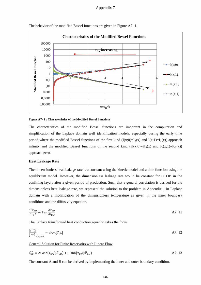
Appendix 7
The behavior of the modified Bessel functions are given in Figure A7- 1.
Figure A7- 1 : Characteristics of the Modified Bessel Functions
The characteristics of the modified Bessel functions are important in the computation and
simplification of the Laplace domain well identification models, especially during the early time
period where the modified Bessel functions of the first kind (I(x;0)=I0(x) and I(x;1)=I1(x)) approach
infinity and the modified Bessel functions of the second kind (K(x;0)=K0(x) and K(x;1)=K1(x))
approach zero.
Heat Leakage Rate
The dimensionless heat leakage rate is a constant using the kinetic model and a time function using the
equilibrium model. However, the dimensionless leakage rate would be constant for CTOB in the
confining layers after a given period of production. Such that a general correlation is derived for the
dimensionless heat leakage rate, we represent the solution to the problem in Appendix 1 in Laplace
domain with a modification of the dimensionless temperature as given in the inner boundary
conditions and the diffusivity equation.
∂2TpD∂zD2
= FCD∂TpD∂tDw
A7: 11
The Laplace transformed heat conduction equation takes the form:
�∂2TpD�
∂zD2 �
layer2= pFCD�TpD� � A7: 12
General Solution for Finite Reservoirs with Linear Flow
TpD� = ACosh�zD�pFCD� + BSinh�zD�pFCD� A7: 13
The constant A and B can be derived by implementing the inner and outer boundary condition.
0,00001
0,0001
0,001
0,01
0,1
1
10
100
1000
10000
100000
0 1 2 3 4 5 6
Mod
ified
Bes
sel F
unct
ion
x=rD√s
Characteristics of the Modified Bessel Functions
I(x;0)
I(x;1)
K(x;0)
K(x;1)0
∞
tDw increasing
146

Appendix 7
Constant Temperature Outer Boundary (CTOB)
Inner Boundary Condition
From the dimensionless Temperature given in Appendix 6, we get:
TpD(rD, tDw, zD = 1) = � λhd
rw2
h2� �dTeq
dp� 1
k�ρt�krɳ �t
�φD A7: 14
The Laplace transform of the above model is hence:
TpD� (r𝐷𝐷, p, zD = 1) = �� λhd
rw2
h2 � �dTeq
dp �1
k�ρt�krɳ �t
�� φ�D = �� λhd
rw2
h2 � �dTeq
dp �1
kft(p)�φ�D = eDφ�D A7: 15
Outer Boundary Condition
Ti − T(r, t, zD = ∆zD) = 0
Using the boundary conditions above, the general equation takes the form:
TpD� = �Sinh�zD�pFCD�Cosh�∆zD�pFCD�−Sinh�∆zD�pFCD�Cosh�zD�pFCD��Sinh��pFCD�Cosh�∆zD�pFCD�−Sinh�∆zD�pFCD�Cosh��pFCD��
� eDφ�D A7: 16
The above equation can further be simplified thus:
TpD� = �Sinh��pFCD(zD−∆zD)�Sinh��pFCD(1−∆zD)�
� eDφ�D = −�Sinh��pFCD(∆zD−zD)�Sinh��pFCD(∆zD−1)�
� eDφ�D A7: 17
The heat leakage rate to the hydrate layer in Laplace domain is given thus:
QD� = dTpD�
dzD= ��pFCD
Cosh��pFCD(∆zD−zD)�Sinh��pFCD(∆zD−1)�
� eDφ�D A7: 18
At the crossflow point, the above differential is:
dTpD�
dzD= ��pFCD
Cosh��pFCD(∆zD−1)�Sinh��pFCD(∆zD−1)�
� eDφ�D = ��pFCDCoth��pFCD(∆zD − 1)��eDφ�D A7: 19
dTpD�
dzD= ��pFCDCoth��pFCD(∆zD − 1)��eDφ�D A7: 20
dTpD�
dzD= QpD
� eDφ�D A7: 21
Pseudo-No Flow Temperature Boundary (p-NFTB)
The p-NFTB basically considers the effect of temperature drop at the exterior boundary, especially in
the top confining layer which is sensitive to the geothermal profile and decreases with decreasing
depth.
dTD�
dzD= ��pFCDtanh��pFCD(∆zD − 1)��eDφ�D A7: 22
dTD�
dzD= QpD
� eDφ�D A7: 23
147

Appendix 7
General Solution for Infinite Outer Boundary
TD� = Ae−zD�pFCD A7: 24
Using the inner boundary and considering the temperature dependence on the pressure in the hydrate
layer, we get the following general equation:
TD� = �e−zD�pFCD
e−�pFCD� eDφ�D A7: 25
dTD�
dzD= ��pFCD
e−zD�pFCD
e−�pFCD� eDφ�D A7: 26
At the crossflow point, the above differential is:
dTD�
dzD= ��pFCD�eDφ�D A7: 27
dTD�
dzD= QpD
� eDφ�D A7: 28
The general dimensionless heat leakage rate is given by:
γDe = �λ 1
hdk�ρt�krɳ �t
��dTeqdp
� rw2
h2� QpD� = eDQpD
� A7: 29
This could be incorporated in the Laplace transformed diffusivity equation and the solution derived.
This makes the use of the Laplace transformation for such problems very useful.
Hence,
β = rD�SDp + eDQpD� A7: 30
148
Appendix 8
Appendix 8: Boltzmann Transformation of Diffusivity Equation in Class 3 Gas Hydrates
∂2φD∂rD2
+ 1rD
∂φD ∂rD
= SD∂φD∂tDw
A8: 1
The similarity variable for the Boltzmann transformation is given below:
vD2 = SDrD2
4tDw A8: 2
Inserting the above transformations into the diffusivity equation results to the following:
∂2φD∂vD2
+ � 1vD
+ 2vD�∂φD ∂vD
= 0 A8: 3
Note that other representations of the transformed diffusivity equation exist with the similarity
variable defined earlier, however; the solutions to the diffusivity equation are the same.
By introducing the parameter below and separating variables, the general solution to the transient
pseudo-pressure can be derived.
y = dφD dvD
A8: 4
The general solution is hence:
φD = B∫ e−vD2
vDdvD
∞vD
= B2 ∫
e−u
udu∞
u + C = B2
[E1(vD2)] A8: 5
The derivative of the E1-function as given by Abramowitz and Stegun [80] is:
dE1(vD2)
dvD2= −e−vD
2
vD2 A8: 6
General Solution for negligible heat influx (Exponential Integral Function)
φD = B2
[E1(vD2)] A8: 7
General Solution for Finite Reservoirs Using the Image Well Theory
The well image theory proposed by [41] is the most widely used method in reservoir engineering to
investigate the influence of sealing faults and recharge at reservoir boundaries. The method simply
involves the application of the superposition principle of the pressure drop from an image well
opposite the production well where the boundary is located. With this method, multiple boundaries can
be incorporated at different distances from the producing well and hence the reservoir response
estimated. Using the line source image well theory with constant rate inner boundary, the general well
response can be defined thus [41], [81]:
φD = φD,pumped ± ∑ φDimage,ini=1 A8: 8
φD = B2�E1(vD2) ±∑ E1 �
SD�2lD,i−rD�2
4tDw�n
i=1 � A8: 9
149
Appendix 8
2lD denotes the dimensionless distance between the producing well and the image well for the
boundary in question. For a recharging image well (constant pressure outer boundary), the negative
sign is valid and for no-flow boundaries (sealing boundary), the plus sign is valid. Note that using the
image well, theory, the inner boundary conditions in the producing well are still imposed. Methods of
incorporating multiple boundaries have also been given by [41], [81] however; reservoir responses
with just single boundaries at different distances from the producing well will be developed using the
similarity solutions. Solutions for confined reservoirs will be given using the Laplace transform.
Finite Wellbore Image Well Theory for Single Boundary Reservoirs
The model presented by [41] describes the line source solution of the reservoir response which needs
modifications when handling finite wellbore problems. In a similar manner, we develop the models for
the finite wellbore case for both CPIB and CRIB. The general solution for this case is given thus:
φD = �AE1(vD2) + BE1 �SD(2lD−rD)2
4tDw�� A8: 10
The image well theory can also be applied to the Laplace domain solutions to investigate the effects of
a single boundary on the reservoir response, as also seen in the works of [82]. The general equation for
the image well theory in Laplace domain is given thus:
φ�D = AK0�rD√𝑉𝑉�+ BK0 �(2lD − rD)√𝑉𝑉� A8: 11
Case 1: Constant Pressure Inner Boundary
Case 1a: CPIB and CPOB
CPIB
φD = 1 = AE1 �SD1
4tDw�+ BE1 �SD
(2lD−1)2
4tDw� A8: 12
CPOB
φD = 0 = AE1 �SDlD2
4tDw� + BE1 �SD
lD2
4tDw� A8: 13
A = −B
φD = �E1�SD
rD2
4tDw�−E1�
SD�2lD−rD�2
4tDw�
E1�SD1
4tDw�−E1�SD
�2lD−1�2
4tDw�� A8: 14
In Laplace Domain, this is given thus:
φ�D = √𝑠𝑠𝐶𝐶�K0�rD√𝑠𝑠�−K0�(2lD−rD)√𝑠𝑠�
K0�√𝑠𝑠�−K0�(2lD−1)√𝑠𝑠�� A8: 15
150
Appendix 8
Case 1b: CPIB and NFB
CPIB
φD = 1 = AE1 �SD1
4tDw� + BE1 �SD
(2lD−1)2
4tDw� A8: 16
NFB
�dφDdrD
�rD
= −A �2SDrD4tDw
e−�SD
rD24tDw
�
�SD𝑟𝑟D2
4tDw�� + B
⎣⎢⎢⎢⎡2SD(2lD−rD)
4tDw
e−�
SD�2lD−rD�2
4tDw�
�SD�2lD−rD�
2
4tDw�⎦⎥⎥⎥⎤ A8: 17
�dφDdrD
�rD=lD
= 0 = −A
⎣⎢⎢⎢⎡2 e
−�SDlD
2
4tDw�
𝑙𝑙D
⎦⎥⎥⎥⎤
+ B
⎣⎢⎢⎢⎡2 e
−�SDlD
2
4tDw�
𝑙𝑙D
⎦⎥⎥⎥⎤ A8: 18
A = B
φD = �E1�SD
rD2
4tDw�+E1�
SD�2lD−rD�2
4tDw�
E1�SD1
4tDw�+E1�SD
�2lD−1�2
4tDw�� A8: 19
In Laplace domain, this is given thus:
φ�D = √𝑠𝑠𝐶𝐶�K0�rD√𝑠𝑠�+K0�(2lD−rD)√𝑠𝑠�
K0�√𝑠𝑠�+K0�(2lD−1)√𝑠𝑠�� A8: 20
Case 2: Constant Rate Inner Boundary
Case 2a: CRIB and CPOB
CPOB
φD = 0 = AE1 �−SDreD2
4tDw�+ BE1 �−SD
lD2
4tDw� A8: 21
A = −B
−rD �dφDdrD
�rD
= rDA
⎩⎪⎨
⎪⎧
�2 e−�SD
rD2
4tDw�
𝑟𝑟D� +
⎣⎢⎢⎢⎡2 e
−�SD�2lD−rD�
2
4tDw�
(2lD−rD)
⎦⎥⎥⎥⎤
⎭⎪⎬
⎪⎫
A8: 22
1 = −rDdφDdrD
= mtD = 2A
⎩⎪⎨
⎪⎧
e−�SD1
4tDw� +
⎣⎢⎢⎢⎡e−⎝
⎛SD�2lD−1�
2
4tDw⎠
⎞
�2lD−1�
⎦⎥⎥⎥⎤
⎭⎪⎬
⎪⎫
A8: 23
A = 12
1
⎩⎪⎪⎨
⎪⎪⎧
e−�SD
14tDw
�+
⎣⎢⎢⎢⎢⎢⎡
e−⎝
⎛SD�2lD−1�
2
4tDw⎠
⎞
�2lD−1�
⎦⎥⎥⎥⎥⎥⎤
⎭⎪⎪⎬
⎪⎪⎫ A8: 24
151
Appendix 8
If the well is produced long enough and the distance to the boundary is relatively far from the
wellbore, the above coefficient takes the line source approximation, i.e.:
A = 12
1
⎩⎪⎪⎨
⎪⎪⎧
e−�SD
14tDw
�+
⎣⎢⎢⎢⎢⎢⎡
e−⎝
⎛SD�2lD−1�
2
4tDw⎠
⎞
�2lD−1�
⎦⎥⎥⎥⎥⎥⎤
⎭⎪⎪⎬
⎪⎪⎫≈ 1
2 A8: 25
φD = 1
2
1
⎩⎪⎨
⎪⎧
e−�SD
14tDw
�+
⎣⎢⎢⎢⎡e−�
SD�2lD−1�2
4tDw�
�2lD−1�
⎦⎥⎥⎥⎤
⎭⎪⎬
⎪⎫�E1 �SD
rD2
4tDw� − E1 �
SD(2lD−rD)2
4tDw�� A8: 26
In Laplace domain, this is given thus:
φ�D = 1𝐶𝐶√𝑠𝑠
�K0�rD√𝑠𝑠�−K0�(2lD−rD)√𝑠𝑠�
K1�√𝑠𝑠�+K1�(2lD−1)√𝑠𝑠�� A8: 27
Case 2b: CRIB and NFB
By applying the same methodology we get the following representation for the reservoir response:
φD = 1
2
1
⎩⎪⎨
⎪⎧
e−�SD
14tDw
�+
⎣⎢⎢⎢⎡e−�
SD�2lD−1�2
4tDw�
�2lD−1�
⎦⎥⎥⎥⎤
⎭⎪⎬
⎪⎫�E1 �SD
rD2
4tDw� + E1 �
SD(2lD−rD)2
4tDw�� A8: 28
In Laplace domain, this is given thus:
φ�D = 1𝐶𝐶√𝑠𝑠
�K0�rD√𝑠𝑠�+K0�(2lD−rD)√𝑠𝑠�
K1�√𝑠𝑠�−K1�(2lD−1)√𝑠𝑠�� A8: 29
152
Appendix 9
Appendix 9: Definition of pseudo-gas relative permeability for rate and pressure
transient analyses (MBM)
As defined earlier, the pseudo-pressure model is developed based on mass balance techniques, which
could be split to different fluid components. In performing well test analysis for the multiphase
system, such that effective permeability changes during production are quantified, it is important to
break down the pseudo-pressure model for each phase such that the conventional pseudo-pressure
model in gas reservoirs can be used. This is done thus:
∫ �krg∗ � �ρgɳg
dp�𝐶𝐶𝑖𝑖𝐶𝐶 = ∫ Udv𝐶𝐶𝑖𝑖
𝐶𝐶 A9: 1
After integrating by parts we get:
∫ �krg∗ � �ρgɳg
dp�𝐶𝐶𝑖𝑖𝐶𝐶 = krg∗ (p)∫
ρgɳg
dp𝐶𝐶𝑖𝑖𝐶𝐶 A9: 2
Where,
krg∗ (p) = �krg∗ �𝐶𝐶𝐶𝐶𝑖𝑖 −
∫ ��∫ρgɳgdp𝑝𝑝𝑖𝑖
𝑝𝑝 �d�krg∗ ��𝑈𝑈𝐶𝐶𝑝𝑝𝑖𝑖𝑝𝑝
∫ρgɳgdp𝑝𝑝𝑖𝑖
𝑝𝑝� A9: 3
The pseudo-pressure integral function for the gas phase reduces then to:
∫ �krg∗ � �ρgɳg
dp�𝐶𝐶𝑖𝑖𝐶𝐶 = krg∗ (p)∫
ρgɳg
dp𝐶𝐶𝑖𝑖𝐶𝐶 = krg∗ (p)ρg,st ∫
dp𝐵𝐵gɳg
𝐶𝐶𝑖𝑖𝐶𝐶 A9: 4
With the above approximate solution of the pseudo-pressure integral, rate transient analysis for the gas
phase becomes easier as the approximate solution to the pseudo-pressure integral is very much easier
to compute.
Note that for ideal reservoir response, the relative permeability term is pressure independent, i.e.:
∫ �krg∗ � �ρgɳg
dp�𝐶𝐶𝑖𝑖𝐶𝐶 = �krg∗ � ∫
ρgɳg
dp𝐶𝐶𝑖𝑖𝐶𝐶 A9: 5
153
Appendix 10
Appendix 10: Apparent Effective Gas Permeability for Multiphase Flow in Gas
Hydrates and Derivatives
Kome et al [48] introduced the equivalent average effective permeability (or just apparent effective
permeability) for heterogeneous reservoir behavior which is also applied here. The use of this model is
applicable to gas class 3 gas hydrate reservoirs with negligible heat flux through conduction. The gas
phase is analyzed. The methodology applied by [48] is based on the derivative analysis used for
reservoir diagnosis. Before addressing the model of the equivalent average effective permeability, the
methods used in derivative analysis are addressed first.
Rate and Pressure Transient Derivatives
It is simply the differential of the solutions presented for rate or pressure transient with respect to time
and is usually computed using the finite difference quotient method as given by [22], [83] and can be
computed for RTA and PTA thus:
Der (RTA) = tDwd� 1
mtD�
dtDw=
d� 1mtD
�
dlntDw A10: 1
Der(PTA) = tDwd(φD)dtDw
= d(φD)dlntDw
A10: 2
Bourdet Differentiation Algorithm
Der (PTA) =�
��φD�n+2−�φD�n+1�
��lntDw�n+2−�lntDw�n+1�[(lntDw)n+1−(lntDw)n]�+�
��φD�n+1−�φD�n�
��lntDw�n+1−�lntDw�n�[(lntDw)n+2−(lntDw)n+1]�
[(lntDw)n+2−(lntDw)n+1]+[(lntDw)n+1−(lntDw)n] A10: 3
Der (RTA) =
��� 1mtD
�n+2
−� 1mtD
�n+1
�
��lntDw�n+2−�lntDw�n+1�[(lntDw)n+1−(lntDw)n]�+�
�� 1mtD
�n+1
−� 1mtD
�n�
��lntDw�n+1−�lntDw�n�[(lntDw)n+2−(lntDw)n+1]�
[(lntDw)n+2−(lntDw)n+1]+[(lntDw)n+1−(lntDw)n] A10: 4
The smoothness of the Bourdet derivative above is dependent on the consistency of the time spacing
and would hence show a significant deviation from the exact derivative solutions.
Exact Derivative
The exact derivative of the pressure transient solutions can be represented in terms of the generalized
incomplete gamma function given in Appendix 18 as will be seen later in the solutions to the
diffusivity equation.
dΓ(a,µ;β)dtDw
= dΓ(a,µ;β)dx
∗ dxdtDw
= − 1x1−a exp �−x− β2
4x� ∗dx
dtDw A10: 5
Der (PTA) = tDwdΓ(a,µ;β)dtDw
= − tDwx1−a exp �−x − β2
4x� ∗dx
dtDw A10: 6
Conventionally, β represents the influx of mass or increase in saturation in the system. Hence, for all
values of β>0, the system characterizes an increase in saturation which is also reflected in the effective
permeability of the phases.
154
Appendix 10
To address the changes in the effective permeability during production, the gas pseudo-pressure
normalized rate representation is used and the derivative during infinite acting radial flow could be
represented thus:
∆ � ∆φQg,st
� = ∆�φRPI(t)�∆lnt
= 0.5pstπhkg,avg
∗ Tst[ln(t2) − ln(t1)] A10: 7
Der =∆� ∆φ
Qg,st�
∆lnt= 0.5pst
πhkg,avg∗ Tst
A10: 8
kg,avg∗ = 0.5pst
πhDerTst A10: 9
kg,avg∗ =
kg2∗ kg1∗ [ln(t2)−ln(t1)]
kg1∗ �ln��ρt�
krɳ �t
�id
rw2�ρcT�eff,id
t2SD2
�+0.80907�−kg2∗ �ln��ρt�
krɳ �t
�id
rw2�ρcT�eff,id
t1SD1
�+0.80907�
A10: 10
The above equation could be simplified by introducing an apparent dimensionless pseudo-skin
component thus:
kg,avg∗ = kg1∗
ln�t2t1�
sDa+ln��t2SD2
�
kg1∗
kg2∗∗SD1t1
�
A10: 11
Where,
sDa = �kg1∗
kg2∗− 1� �ln�
�ρt�krɳ �t
�id
rw2(ρcT)eff,id� + 0.80907� A10: 12
Under ideal conditions, k g1* = k g2
* and SD1=SD2, hence:
kg,avg∗ = kg1∗
ln�t2t1�
ln�t2t1�
= kg1∗ A10: 13
The derivative is therefore a very powerful tool in addressing changes in reservoir behavior or
permeability which has also been addressed in detail in the works of [84], [85], [86], [65], [66] ,
whereby derivative plots have been used to derive reservoir parameters with the application of the
Tiabs Direct Synthesis (TDS) Technique.
155
Appendix 11
Appendix 11: Multiphase Crossflow Storativity Transformations
To account for the storativity of the two layers involved in crossflow behavior, the storativity ratio as
given by Warren and Root [87] is usually used. In a similar manner, the storativity ratio for the hydrate
and free fluid layer are developed here.
ω∗ + (1 − 𝜔𝜔∗) = avah+av
+ ahah+av
= 1 A11: 1
The storativity in the crossflow layer is given thus:
1av
= (1 −ω∗) � 1ah
+ 1av� A11: 2
1av
= (1 −ω) ��ah+avahav
��i A11: 3
Similarly, the same can be done for the producing layer thus:
1ah
= ω∗ � 1ah
+ 1av� A11: 4
1ah
= ω ��ah+avahav
��i A11: 5
Where,
ω∗ = avah+av
A11: 6
(1 −ω∗) = ahah+av
A11: 7
Storativity Ratio
(1 −ω) = (1 −ω∗)��ah+avahav
��
��ah+avahav��i
= 1av
1
��ah+avahav��i
= [av]𝑖𝑖av
�� ahah+av
��i A11: 8
ω = ω∗��ah+avahav
��
��ah+avahav��i
= 1ah
1
��ah+avahav��i
= [ah]𝑖𝑖ah
�� avah+av
��i A11: 9
ahav
= (1−ω)ω
A11: 10
Interporosity Flow Coefficient
δD = rw2
∆z2∆z1
kv2kh1
A11: 11
156
Appendix 12
Appendix 12: Analytical Solutions to Diffusivity Problems in Normally Pressured Gas
Hydrates
Diffusivity Equation with Negligible Heat Influx
∂2φD∂rD2
+ 1rD
∂φD ∂rD
= SD∂φD∂tDw
A12: 1
The solutions to the above equation will be presented using the Boltzmann transformation (similarity
solutions)
Diffusivity Equation with considerable Heat Influx
∂2φD∂rD2
+ 1rD
∂φD ∂rD
− γDeφD = SD∂φD∂tDw
A12: 2
Diffusivity Equation with Kinetic Model
∂2φD∂rD2
+ 1rD
∂φD ∂rD
− γDkφD = SDk∂φD∂tDw
A12: 3
Case 1: Constant Pressure Inner Boundary Solutions
General Similarity Solution
φD = B2
E1(vD2) = B2
E1 �rD2
4tDwSD� A12: 4
Case 1a: Infinite Acting Reservoirs: Constant Pressure Inner Boundary Conditions
φD(rD, tDw) = 1 at rD=1 and tDw>0 vD2 = SD4tDw
For the above inner boundary condition, the constant B can be derived thus:
1
E1�1
4tDw�
= B2 A12: 5
Dimensionless Pseudo-Pressure
φD(rD, tDw) = φ(r,t)−φiφwf−φi
=�E1�SD
rD2
4tDw��
�E1�SD
4tDw��
A12: 6
Transient Rate
mtD = −rDdφDdrD
= −2vD2dφDdvD
2 = −2vD21
�E1�SD
4tDw��
d��E1�vD2 ���
dvD2 A12: 7
Using the differential of the E1-function as given by [80] we get:
mtD = 2e−vD2
�E1�SD
4tDw��
A12: 8
157
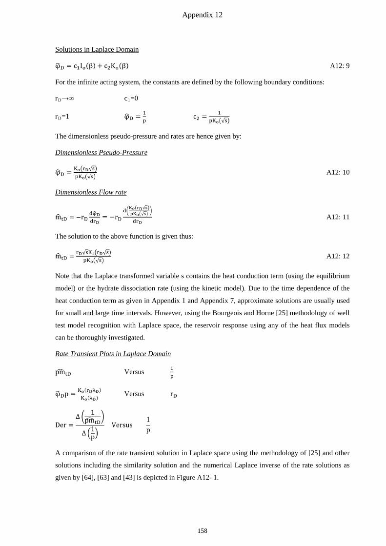
Appendix 12
Solutions in Laplace Domain
φ�D = c1Io(β) + c2Ko(β) A12: 9
For the infinite acting system, the constants are defined by the following boundary conditions:
rD→∞ c1=0
rD=1 φ�D = 1p c2 = 1
pKo�√s�
The dimensionless pseudo-pressure and rates are hence given by:
Dimensionless Pseudo-Pressure
φ�D = Ko�rD√s�pKo�√s�
A12: 10
Dimensionless Flow rate
m� tD = −rDdφ�DdrD
= −rDd�Ko�rD√s�pKo�√s�
�
drD A12: 11
The solution to the above function is given thus:
m� tD =rD√sK1�rD√s�
pKo�√s� A12: 12
Note that the Laplace transformed variable s contains the heat conduction term (using the equilibrium
model) or the hydrate dissociation rate (using the kinetic model). Due to the time dependence of the
heat conduction term as given in Appendix 1 and Appendix 7, approximate solutions are usually used
for small and large time intervals. However, using the Bourgeois and Horne [25] methodology of well
test model recognition with Laplace space, the reservoir response using any of the heat flux models
can be thoroughly investigated.
Rate Transient Plots in Laplace Domain
pm� tD Versus 1p
φ�Dp = Ko(rDλD)Ko(λD) Versus rD
Der =∆ � 1
pm� tD�
∆ �1p�
Versus 1p
A comparison of the rate transient solution in Laplace space using the methodology of [25] and other
solutions including the similarity solution and the numerical Laplace inverse of the rate solutions as
given by [64], [63] and [43] is depicted in Figure A12- 1.
158
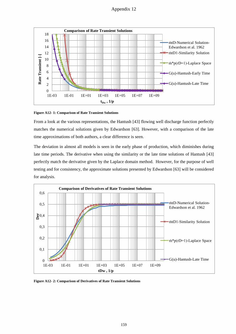
Appendix 12
Figure A12- 1: Comparison of Rate Transient Solutions
From a look at the various representations, the Hantush [43] flowing well discharge function perfectly
matches the numerical solutions given by Edwardson [63]. However, with a comparison of the late
time approximations of both authors, a clear difference is seen.
The deviation in almost all models is seen in the early phase of production, which diminishes during
late time periods. The derivative when using the similarity or the late time solutions of Hantush [43]
perfectly match the derivative given by the Laplace domain method. However, for the purpose of well
testing and for consistency, the approximate solutions presented by Edwardson [63] will be considered
for analysis.
Figure A12- 2: Comparison of Derivatives of Rate Transient Solutions
02468
1012141618
1E-03 1E-01 1E+01 1E+03 1E+05 1E+07 1E+09
Rat
e T
rans
ient
[-]
tDw , 1/p
Comparison of Rate Transient Solutions
ṁtD-Numerical Solution- Edwardson et al. 1962 ṁtD1-Similarity Solution
ṁ*p(rD=1)-Laplace Space
G(u)-Hantush-Early Time
G(u)-Hantush-Late Time
0
0,1
0,2
0,3
0,4
0,5
0,6
1E-03 1E-01 1E+01 1E+03 1E+05 1E+07 1E+09
Der
tDw , 1/p
Comparison of Derivatives of Rate Transient Solutions
ṁtD-Numerical Solution- Edwardson et al. 1962
ṁtD1-Similarity Solution
ṁ*p(rD=1)-Laplace Space
G(u)-Hantush-Late Time
159
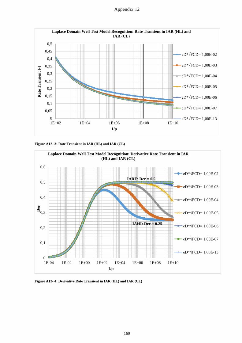
Appendix 12
Figure A12- 3: Rate Transient in IAR (HL) and IAR (CL)
Figure A12- 4: Derivative Rate Transient in IAR (HL) and IAR (CL)
0
0,05
0,1
0,15
0,2
0,25
0,3
0,35
0,4
0,45
0,5
1E+02 1E+04 1E+06 1E+08 1E+10
Rat
e T
rans
ient
[-]
1/p
Laplace Domain Well Test Model Recognition: Rate Transient in IAR (HL) and IAR (CL)
eD*√FCD= 1,00E-02
eD*√FCD= 1,00E-03
eD*√FCD= 1,00E-04
eD*√FCD= 1,00E-05
eD*√FCD= 1,00E-06
eD*√FCD= 1,00E-07
eD*√FCD= 1,00E-13
0
0,1
0,2
0,3
0,4
0,5
0,6
1E-04 1E-02 1E+00 1E+02 1E+04 1E+06 1E+08 1E+10
Der
1/p
Laplace Domain Well Test Model Recognition: Derivative Rate Transient in IAR (HL) and IAR (CL)
eD*√FCD= 1,00E-02
eD*√FCD= 1,00E-03
eD*√FCD= 1,00E-04
eD*√FCD= 1,00E-05
eD*√FCD= 1,00E-06
eD*√FCD= 1,00E-07
eD*√FCD= 1,00E-13
IARF: Der = 0.5
IAHI: Der = 0.25
160
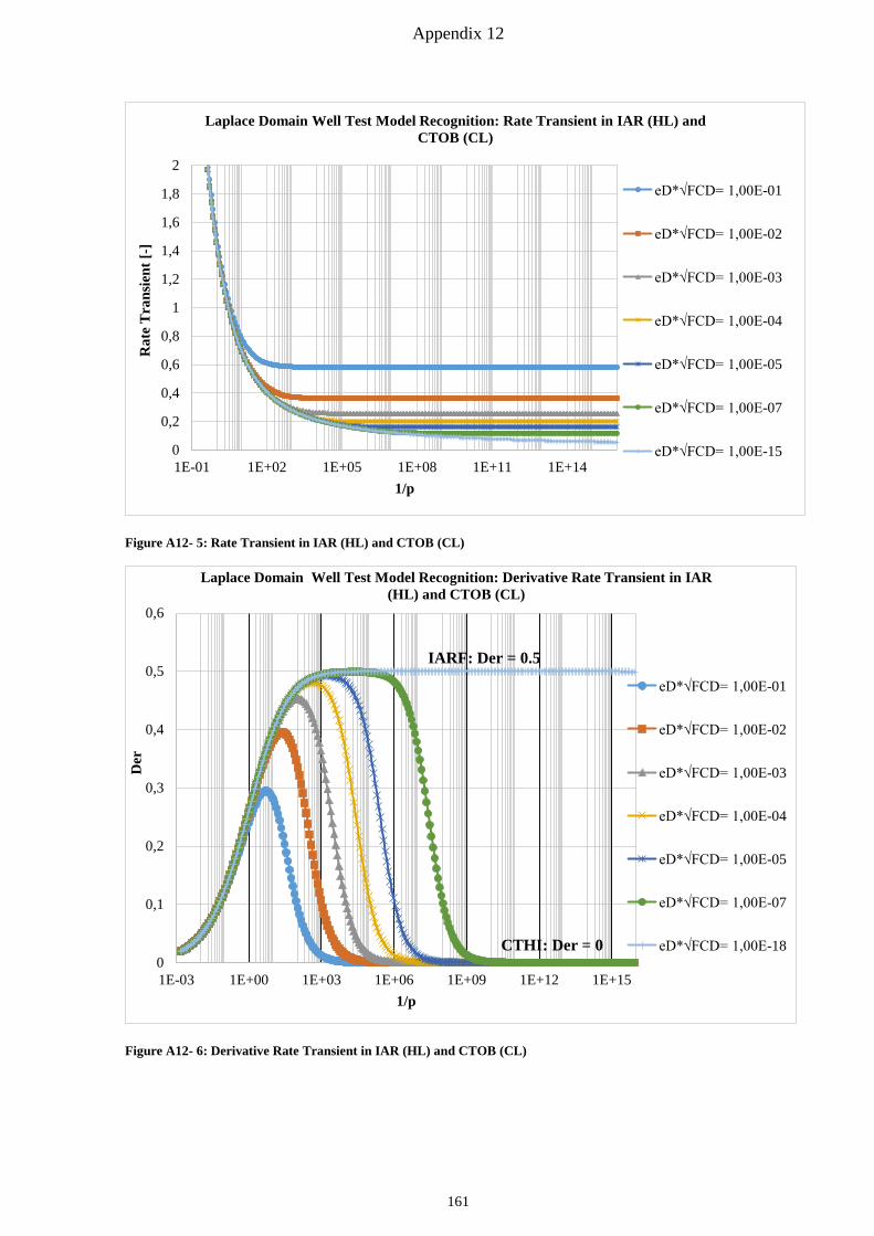
Appendix 12
Figure A12- 5: Rate Transient in IAR (HL) and CTOB (CL)
Figure A12- 6: Derivative Rate Transient in IAR (HL) and CTOB (CL)
0
0,2
0,4
0,6
0,8
1
1,2
1,4
1,6
1,8
2
1E-01 1E+02 1E+05 1E+08 1E+11 1E+14
Rat
e T
rans
ient
[-]
1/p
Laplace Domain Well Test Model Recognition: Rate Transient in IAR (HL) and CTOB (CL)
eD*√FCD= 1,00E-01
eD*√FCD= 1,00E-02
eD*√FCD= 1,00E-03
eD*√FCD= 1,00E-04
eD*√FCD= 1,00E-05
eD*√FCD= 1,00E-07
eD*√FCD= 1,00E-15
0
0,1
0,2
0,3
0,4
0,5
0,6
1E-03 1E+00 1E+03 1E+06 1E+09 1E+12 1E+15
Der
1/p
Laplace Domain Well Test Model Recognition: Derivative Rate Transient in IAR (HL) and CTOB (CL)
eD*√FCD= 1,00E-01
eD*√FCD= 1,00E-02
eD*√FCD= 1,00E-03
eD*√FCD= 1,00E-04
eD*√FCD= 1,00E-05
eD*√FCD= 1,00E-07
eD*√FCD= 1,00E-18
IARF: Der = 0.5
CTHI: Der = 0
161

Appendix 12
Figure A12- 7: Rate Transient in IAR (HL) and CTOB (CL) and Effects of Thickness of CL
Figure A12- 8: Rate Transient Derivative in IAR (HL) and CTOB (CL) and Effects of Thickness of CL
0
0,1
0,2
0,3
0,4
0,5
0,6
0,7
0,8
0,9
1
1E-03 1E+00 1E+03 1E+06 1E+09 1E+12
Rat
e T
rans
ient
[-]
1/p
Laplace Domain Well Test Model Recognition: Rate Transient in IAR (HL) and CTOB (CL) with Effects of Thickness of CL (eD√FCD = 3.16E-03)
ΔzD 2,00E+05
ΔzD 2,00E+03
ΔzD 2,00E+01
0
0,1
0,2
0,3
0,4
0,5
0,6
0,7
1E-03 1E+00 1E+03 1E+06 1E+09 1E+12
Der
1/p
Laplace Domain Well Test Model Recognition: Derivative Rate Transient in IAR (HL) and CTOB (CL) with Effects of Thickness of CL (eD√FCD = 3.16E-03)
ΔzD 2,00E+05
ΔzD 2,00E+03
ΔzD 2,00E+01
162
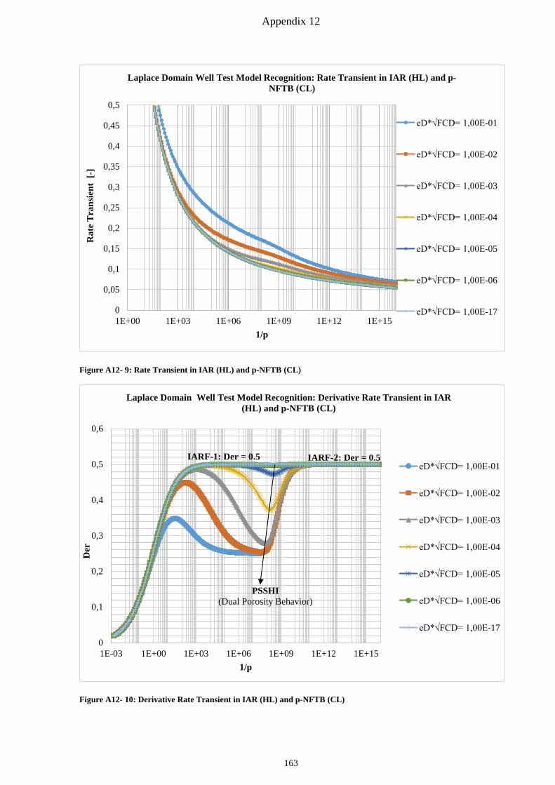
Appendix 12
Figure A12- 9: Rate Transient in IAR (HL) and p-NFTB (CL)
Figure A12- 10: Derivative Rate Transient in IAR (HL) and p-NFTB (CL)
0
0,05
0,1
0,15
0,2
0,25
0,3
0,35
0,4
0,45
0,5
1E+00 1E+03 1E+06 1E+09 1E+12 1E+15
Rat
e T
rans
ient
[-]
1/p
Laplace Domain Well Test Model Recognition: Rate Transient in IAR (HL) and p-NFTB (CL)
eD*√FCD= 1,00E-01
eD*√FCD= 1,00E-02
eD*√FCD= 1,00E-03
eD*√FCD= 1,00E-04
eD*√FCD= 1,00E-05
eD*√FCD= 1,00E-06
eD*√FCD= 1,00E-17
0
0,1
0,2
0,3
0,4
0,5
0,6
1E-03 1E+00 1E+03 1E+06 1E+09 1E+12 1E+15
Der
1/p
Laplace Domain Well Test Model Recognition: Derivative Rate Transient in IAR (HL) and p-NFTB (CL)
eD*√FCD= 1,00E-01
eD*√FCD= 1,00E-02
eD*√FCD= 1,00E-03
eD*√FCD= 1,00E-04
eD*√FCD= 1,00E-05
eD*√FCD= 1,00E-06
eD*√FCD= 1,00E-17
IARF-1: Der = 0.5 IARF-2: Der = 0.5
PSSHI (Dual Porosity Behavior)
163
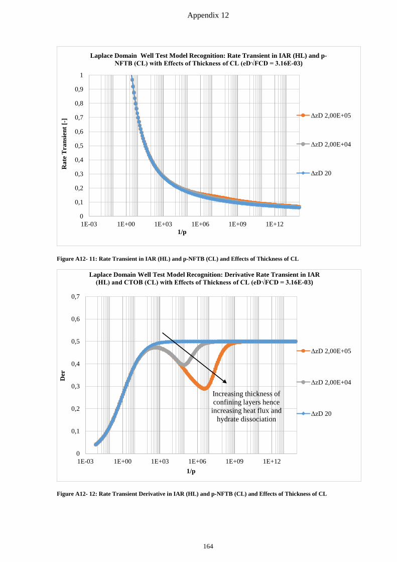
Appendix 12
Figure A12- 11: Rate Transient in IAR (HL) and p-NFTB (CL) and Effects of Thickness of CL
Figure A12- 12: Rate Transient Derivative in IAR (HL) and p-NFTB (CL) and Effects of Thickness of CL
0
0,1
0,2
0,3
0,4
0,5
0,6
0,7
0,8
0,9
1
1E-03 1E+00 1E+03 1E+06 1E+09 1E+12
Rat
e T
rans
ient
[-]
1/p
Laplace Domain Well Test Model Recognition: Rate Transient in IAR (HL) and p-NFTB (CL) with Effects of Thickness of CL (eD√FCD = 3.16E-03)
ΔzD 2,00E+05
ΔzD 2,00E+04
ΔzD 20
0
0,1
0,2
0,3
0,4
0,5
0,6
0,7
1E-03 1E+00 1E+03 1E+06 1E+09 1E+12
Der
1/p
Laplace Domain Well Test Model Recognition: Derivative Rate Transient in IAR (HL) and CTOB (CL) with Effects of Thickness of CL (eD√FCD = 3.16E-03)
ΔzD 2,00E+05
ΔzD 2,00E+04
ΔzD 20
Increasing thickness of confining layers hence
increasing heat flux and hydrate dissociation
164
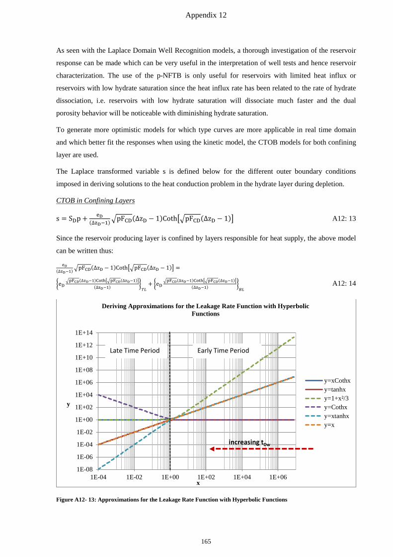
Appendix 12
As seen with the Laplace Domain Well Recognition models, a thorough investigation of the reservoir
response can be made which can be very useful in the interpretation of well tests and hence reservoir
characterization. The use of the p-NFTB is only useful for reservoirs with limited heat influx or
reservoirs with low hydrate saturation since the heat influx rate has been related to the rate of hydrate
dissociation, i.e. reservoirs with low hydrate saturation will dissociate much faster and the dual
porosity behavior will be noticeable with diminishing hydrate saturation.
To generate more optimistic models for which type curves are more applicable in real time domain
and which better fit the responses when using the kinetic model, the CTOB models for both confining
layer are used.
The Laplace transformed variable s is defined below for the different outer boundary conditions
imposed in deriving solutions to the heat conduction problem in the hydrate layer during depletion.
CTOB in Confining Layers
s = SDp + eD(∆zD−1)�pFCD(∆zD − 1)Coth��pFCD(∆zD − 1)� A12: 13
Since the reservoir producing layer is confined by layers responsible for heat supply, the above model
can be written thus:
eD(∆zD−1)�pFCD(∆zD − 1)Coth��pFCD(∆zD − 1)� =
�eD�pFCD(∆zD−1)Coth��pFCD(∆zD−1)�
(∆zD−1) �𝑇𝑇𝐿𝐿
+ �eD�pFCD(∆zD−1)Coth��pFCD(∆zD−1)�
(∆zD−1) �𝐵𝐵𝐿𝐿
A12: 14
Figure A12- 13: Approximations for the Leakage Rate Function with Hyperbolic Functions
1E-08
1E-06
1E-04
1E-02
1E+00
1E+02
1E+04
1E+06
1E+08
1E+10
1E+12
1E+14
1E-04 1E-02 1E+00 1E+02 1E+04 1E+06
y
x
Deriving Approximations for the Leakage Rate Function with Hyperbolic Functions
y=xCothxy=tanhxy=1+x²/3y=Cothxy=xtanhxy=x
increasing tDw
Late Time Period Early Time Period
165
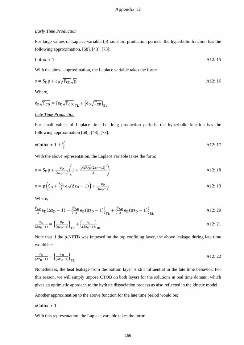
Appendix 12
Early Time Production
For large values of Laplace variable (p) i.e. short production periods, the hyperbolic function has the
following approximation, [68], [43], [73]:
Cothx ≈ 1 A12: 15
With the above approximation, the Laplace variable takes the form:
s = SDp + eD�FCD�p A12: 16
Where,
eD�FCD = �eD�FCD�TL + �eD�FCD�BL
Late Time Production
For small values of Laplace time i.e. long production periods, the hyperbolic function has the
following approximation [68], [43], [73]:
xCothx ≈ 1 + x2
3 A12: 17
With the above representation, the Laplace variable takes the form:
s = SDp + eD(∆zD−1)�1 + ��pFCD(∆zD−1)�
2
3� A12: 18
s = p �SD + FCD3
eD(∆zD − 1)� + eD(∆zD−1) A12: 19
Where,
FCD3
eD(∆zD − 1) = �FCD3
eD(∆zD − 1)�TL
+ �FCD3
eD(∆zD − 1)�BL
A12: 20
eD(∆zD−1) = � eD
(∆zD−1)�TL+ � eD
(∆zD−1)�BL A12: 21
Note that if the p-NFTB was imposed on the top confining layer, the above leakage during late time
would be:
eD(∆zD−1) = � eD
(∆zD−1)�BL A12: 22
Nonetheless, the heat leakage from the bottom layer is still influential in the late time behavior. For
this reason, we will simply impose CTOB on both layers for the solutions in real time domain, which
gives an optimistic approach to the hydrate dissociation process as also reflected in the kinetic model.
Another approximation to the above function for the late time period would be:
xCothx ≈ 1
With this representation, the Laplace variable takes the form:
166
Appendix 12
s = µD2 = pSD + eD(∆zD−1) A12: 23
With the approximations made for early and late time periods, solutions to the diffusivity equation can
also be derived analogue Hantush (1964) and given in the literature [68], [43], [73].
Note that late time approximations could occur at different times in both layers, all depending on the
petrophysical properties of each layer.
Approximate Solutions to the Heat Flux Problem in Time-Domain
Late Time Period for Constant Outer Temperature in Confining Layer
λD = �pSD �1 + FCD3SD
eD(∆zD − 1)� + eD(∆zD−1) = �pSDµD + bD A12: 24
Dimensionless Pseudo-Pressure
φD = 𝐿𝐿−1(φ�D) = 𝐿𝐿−1
⎩⎪⎨
⎪⎧Ko �rD�p�SDµD� + bD�
pKo ��p�SDµD� + bD�⎭⎪⎬
⎪⎫
= Z�tDwSDµD
, rD,�bD�
φD = Z � tDwSDµD
, rD,�bD� = Z� tDw
�1+FCD3SD
eD(∆zD−1)�, rD,�
eD(∆zD−1)� A12: 25
By using the other approximation of the hyperbolic function during the late time period we get:
φD = Z �tDwSD
, rD,�bD� = Z �tDwSD
, rD,�eD
(∆zD−1)� A12: 26
The above flowing well function for leaky aquifers as given by [43] is expressed fully in Appendix 18.
Late Time Approximation for Hydrate Layer:
φD =W�
rD2
4tDwSDµD,rD√bD�
W�SDµD4tDw
,√bD� A12: 27
The above well function for leaky aquifers as given by [43] is expressed fully in Appendix 18.
Dimensionless Flowrate
mtD = 𝐿𝐿−1(m� tD) = 𝐿𝐿−1
⎩⎪⎨
⎪⎧
rD�p�SDµD� + bD
K1 �rD�p�SDµD� + bD�
pKo ��p�SDµD� + bD�⎭⎪⎬
⎪⎫
= G�tDw
SDµD𝑟𝑟𝐷𝐷2 , 𝑟𝑟𝐷𝐷�
eD(∆zD − 1)�
The above flowing well discharge function for leaky aquifers as given by [43] is expressed fully in
Appendix 18.
167
Appendix 12
Dimensionless Flowrate at Wellbore
mtD = G � tDwSDµD
,�eD
(∆zD−1)� A12: 28
By using the other approximation of the hyperbolic function during the late time period we get:
mtD = G �tDwSD
,�eD
(∆zD−1)� A12: 29
In a similar manner, solutions can also be derived using the kinetic model.
The Kinetic Model
s = µD2 = pSDk + γDk A12: 30
φD = Z �tDwSDk
, rD,√γDk� A12: 31
Late Time Approximation for Producing Layer:
φD =W�
rD2
4tDwSDk,rD�γDk�
W� 14tDw
SDk,�γDk� A12: 32
mtD = G �tDwSD
,√γDk� A12: 33
Case 1b: Finite Acting Reservoirs with Constant Pressure Outer Boundary
Constant Pressure Outer Boundary Condition
Similarity Solutions
Using the image well theory discussed in Appendix 8, solutions to the constant pressure outer
boundary problem can be deduced. For a reservoir with one recharge boundary, the reservoir response
can be estimated thus:
Dimensionless Pseudo-Pressure
φD(rD, tDw) =�E1(SD
rD2
4tDw)�−�E1�SD
�2lD−rD�2
4tDw��
�E1( SD4tDw
)�−�E1�SD�2lD−1�
2
4tDw��
A12: 34
Transient Rate
mtD(rD, tDw) = 2 e−�SD
rD2
4tDw�
E1�SD
4tDw�−E1�SD
�2lD−1�2
4tDw�
+ 2 (2lD−rD)−1rDe−�2lD−rD�
2
4tDwSD
E1�SD
4tDw�−E1�SD
�2lD−1�2
4tDw�
A12: 35
mtD(rD = 1, tDw) = 2 e−�
SD4tDw
�+(2lD−1)−1e
−�2lD−1�
2
4tDwSD
E1�SD
4tDw�−E1�SD
�2lD−1�2
4tDw�
A12: 36
168
Appendix 12
Solutions in Laplace Domain
φ�D = c1Io�rD√s� + c2Ko�rD√s� A12: 37
For finite acting reservoirs, the constants c1 is not zero. By imposing the inner and outer boundary
conditions, the solution to the constant pressure outer boundary problem for the confined layer can be
deduced.
reD φ�D = 0
rD=1 φ�D = 1𝐶𝐶
c1 = − 1p� Ko�reD√s�
�Ko�√s�Io�reD√s��−Io�√s�Ko�reD√s�� A12: 38
c2 = 1p� Ko�reD√s�Io�reD√s�
�Ko�√s�Io�reD√s��−Io�√s�Ko�reD√s�� 1Ko�reD√s�
A12: 39
Dimensionless Pseudo-Pressure
φ�D =1p�Ko�rD√s�Io�reD√s� − Ko�reD√s�Io�rD√s�
Io�reD√s�Ko�√s� − Io�√s�Ko�reD√s��
Dimensionless Flow rate
m� tD = rD√sp��K1�rD√s�Io�reD√s�+Ko�reD√s�I1�rD√s��
Io�reD√s�Ko�√s�−Io�√s�Ko�reD√s�� A12: 40
m� tD(rD = 1, p) = √sp�K1�√s�Io�reD√s�+Ko�reD√s�I1�√s�Io�reD√s�Ko�√s�−Io�√s�Ko�reD√s�
� A12: 41
Rate Transient Plot in Laplace Domain
pm� tD Versus 1p
φ�Dp Versus rD
Der =∆ � 1
pm� tD�
∆ �1p�
Versus 1p
For large values of p i.e. early time production period where boundary dominated flow has not been
reached, the reservoir is still acting infinite and from the characteristics of the modified Bessel´s
functions given in Figure A7- 1, the solutions to the infinite acting reservoir are applicable. The image
well theory can also be applied to the solutions in Laplace domain as given in Appendix 8.
169
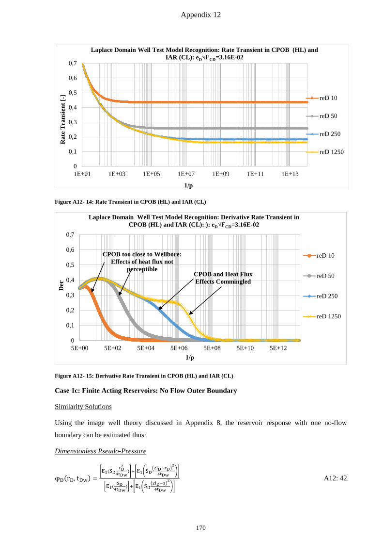
Appendix 12
Figure A12- 14: Rate Transient in CPOB (HL) and IAR (CL)
Figure A12- 15: Derivative Rate Transient in CPOB (HL) and IAR (CL)
Case 1c: Finite Acting Reservoirs: No Flow Outer Boundary
Similarity Solutions
Using the image well theory discussed in Appendix 8, the reservoir response with one no-flow
boundary can be estimated thus:
Dimensionless Pseudo-Pressure
φD(rD, tDw) =�E1(SD
rD2
4tDw)�+�E1�SD
�2lD−rD�2
4tDw��
�E1(SD
4tDw)�+�E1�SD
�2lD−1�2
4tDw��
A12: 42
0
0,1
0,2
0,3
0,4
0,5
0,6
0,7
1E+01 1E+03 1E+05 1E+07 1E+09 1E+11 1E+13
Rat
e T
rans
ient
[-]
1/p
Laplace Domain Well Test Model Recognition: Rate Transient in CPOB (HL) and IAR (CL): eD√FCD=3.16E-02
reD 10
reD 50
reD 250
reD 1250
0
0,1
0,2
0,3
0,4
0,5
0,6
0,7
5E+00 5E+02 5E+04 5E+06 5E+08 5E+10 5E+12
Der
1/p
Laplace Domain Well Test Model Recognition: Derivative Rate Transient in CPOB (HL) and IAR (CL): ): eD√FCD=3.16E-02
reD 10
reD 50
reD 250
reD 1250
CPOB too close to Wellbore: Effects of heat flux not
perceptible CPOB and Heat Flux Effects Commingled
170
Appendix 12
Dimensionless Transient Rate
mtD(rD, tDw) = 2
�e−�
SD4tDw
rD�−(2lD−rD)−1rDe−�2lD−rD�
2
4tDwSD�
�E1(SD
4tDw)�+�E1�SD
�2lD−1�2
4tDw��
A12: 43
mtD(rD = 1, tDw) = 2
�e−�
SD4tDw
�−(2lD−1)−1e
−�2lD−1�
2
4tDwSD�
�E1(SD
4tDw)�+�E1�SD
�2lD−1�2
4tDw��
A12: 44
Solutions in Laplace Domain
φ�D = c1Io�rD√s� + c2Ko�rD√s�
For finite acting reservoirs, the constants c1 is not zero. For constant inner pressure and no-flow outer
boundary conditions, the above equation is:
reD �dφ�DdrD
�reD
= 0 �dφ�DdrD
�reD
= c1√sI1�reD√s� − c2√sK1�reD√s� = 0
rD=1 φ�D = 1p
With the above boundary conditions, the constants c1 and c2 are given thus:
c1 = 1p� K1�reD√s�Ko�√s�I1�reD√s�+K1�reD√s�Io�√s�
� A12: 45
c2 = 1p� K1�reD√s�Ko�√s�I1�reD√s�+K1�reD√s�Io�√s�
� I1�reD√s�K1�reD√s�
A12: 46
Dimensionless Pseudo-Pressure
φ�D = 1p�K1�reD√s�Io�rD√s�+I1�reD√s�Ko�rD√s�
Ko�√s�I1�reD√s�+K1�reD√s�Io�√s�� A12: 47
Dimensionless Flow rate
m� tD = rD√sp��I1�reD√s�K1�rD√s�−K1�reD√s�I1�rD√s��
Ko�√s�I1�reD√s�+K1�reD√s�Io�√s�� A12: 48
m� tD(rD = 1, p) = √sp��I1�reD√s�K1�√s�−K1�reD√s�I1�√s��Ko�√s�I1�reD√s�+K1�reD√s�Io�√s�
� A12: 49
Rate Transient Plot in Laplace Domain
pm� tD Versus 1p
φ�Dp Versus rD
171
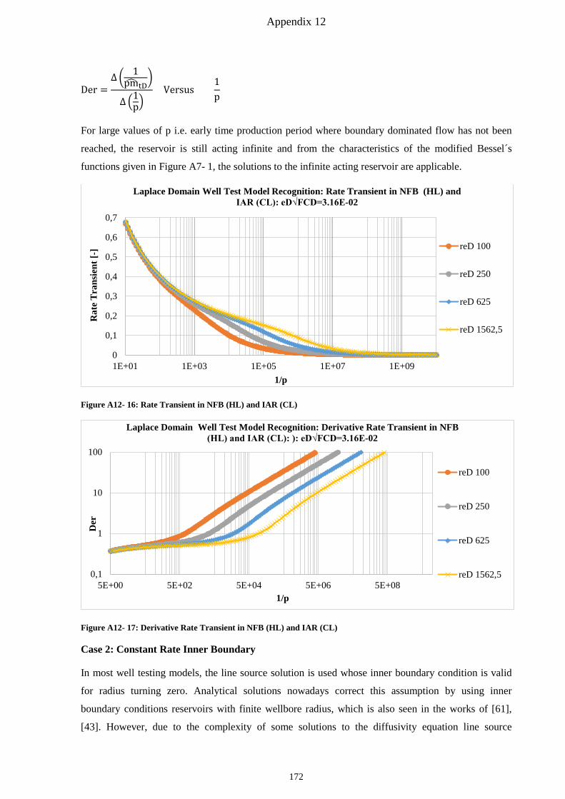
Appendix 12
Der =∆ � 1
pm� tD�
∆ �1p�
Versus 1p
For large values of p i.e. early time production period where boundary dominated flow has not been
reached, the reservoir is still acting infinite and from the characteristics of the modified Bessel´s
functions given in Figure A7- 1, the solutions to the infinite acting reservoir are applicable.
Figure A12- 16: Rate Transient in NFB (HL) and IAR (CL)
Figure A12- 17: Derivative Rate Transient in NFB (HL) and IAR (CL)
Case 2: Constant Rate Inner Boundary
In most well testing models, the line source solution is used whose inner boundary condition is valid
for radius turning zero. Analytical solutions nowadays correct this assumption by using inner
boundary conditions reservoirs with finite wellbore radius, which is also seen in the works of [61],
[43]. However, due to the complexity of some solutions to the diffusivity equation line source
0
0,1
0,2
0,3
0,4
0,5
0,6
0,7
1E+01 1E+03 1E+05 1E+07 1E+09
Rat
e T
rans
ient
[-]
1/p
Laplace Domain Well Test Model Recognition: Rate Transient in NFB (HL) and IAR (CL): eD√FCD=3.16E-02
reD 100
reD 250
reD 625
reD 1562,5
0,1
1
10
100
5E+00 5E+02 5E+04 5E+06 5E+08
Der
1/p
Laplace Domain Well Test Model Recognition: Derivative Rate Transient in NFB (HL) and IAR (CL): ): eD√FCD=3.16E-02
reD 100
reD 250
reD 625
reD 1562,5
172
Appendix 12
assumptions are imposed such that the inverse Laplace transform of the solution is deduced, as will be
seen later.
Case 2a: Infinite Acting
Similarity Solution
φD =B2
E1(vD2)
Inner Boundary Condition
rD∂φD∂rD
= −1 at rD → 1 vD →SD4tDw
From the inner boundary condition, the constant B is given thus:
B = eSD
4tDw A12: 50
φD(rD, tDw) = 12
e1
4tDwE1 �SDrD2
4tDw� A12: 51
Notice the similarity between the CPIB solution and the CRIB which are simply related thus:
φD(rD = 1, tDw) = 1mtD(rD=1,tDw) A12: 52
φwf(rD, tDw) = φi −mt4πhk
�eSD
4tDwE1(SDrD2
4tDw)� A12: 53
φwf(rD = 1, tDw) = φi −mt4πhk
�eSD
4tDwE1( SD4tDw
)� A12: 54
Solution in Laplace Domain
φ�D = c1Io�rD√s� + c2Ko�rD√s�
By transforming the Neumann boundary conditions in Laplace domain, the solution to the Bessel
equation results to:
rD→∞ c1=0
rD=1 m� tD = rDdφ�DdrD
= − 1p c2 = 1
p�√sK1�√s��
The final equation is hence:
φ�D = Ko�rD√s�p�√sK1�√s��
A12: 55
Pseudo-Pressure Transient Plot in Laplace Domain
φ�Dp =Ko�rD√s�√sK1�√s�
=1
𝑝𝑝m� tD
173
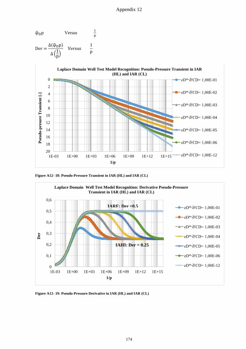
Appendix 12
φ�Dp Versus 1p
Der =∆(φ�Dp)
∆ �1p�
Versus 1p
Figure A12- 18: Pseudo-Pressure Transient in IAR (HL) and IAR (CL)
Figure A12- 19: Pseudo-Pressure Derivative in IAR (HL) and IAR (CL)
0
2
4
6
8
10
12
14
16
18
201E-03 1E+00 1E+03 1E+06 1E+09 1E+12 1E+15
Pseu
do-p
resu
re T
rans
ient
[-]
1/p
Laplace Domain Well Test Model Recognition: Pseudo-Pressure Transient in IAR (HL) and IAR (CL)
eD*√FCD= 1,00E-01
eD*√FCD= 1,00E-02
eD*√FCD= 1,00E-03
eD*√FCD= 1,00E-04
eD*√FCD= 1,00E-05
eD*√FCD= 1,00E-06
eD*√FCD= 1,00E-12
0
0,1
0,2
0,3
0,4
0,5
0,6
1E-03 1E+00 1E+03 1E+06 1E+09 1E+12 1E+15
Der
1/p
Laplace Domain Well Test Model Recognition: Derivative Pseudo-Pressure Transient in IAR (HL) and IAR (CL)
eD*√FCD= 1,00E-01
eD*√FCD= 1,00E-02
eD*√FCD= 1,00E-03
eD*√FCD= 1,00E-04
eD*√FCD= 1,00E-05
eD*√FCD= 1,00E-06
eD*√FCD= 1,00E-12
IARF: Der =0.5
IAHI: Der = 0.25
174
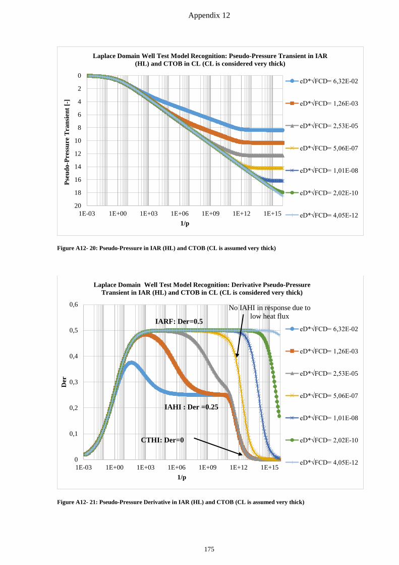
Appendix 12
Figure A12- 20: Pseudo-Pressure in IAR (HL) and CTOB (CL is assumed very thick)
Figure A12- 21: Pseudo-Pressure Derivative in IAR (HL) and CTOB (CL is assumed very thick)
0
2
4
6
8
10
12
14
16
18
201E-03 1E+00 1E+03 1E+06 1E+09 1E+12 1E+15
Pseu
do-P
ress
ure
Tra
nsie
nt [-
]
1/p
Laplace Domain Well Test Model Recognition: Pseudo-Pressure Transient in IAR (HL) and CTOB in CL (CL is considered very thick)
eD*√FCD= 6,32E-02
eD*√FCD= 1,26E-03
eD*√FCD= 2,53E-05
eD*√FCD= 5,06E-07
eD*√FCD= 1,01E-08
eD*√FCD= 2,02E-10
eD*√FCD= 4,05E-12
0
0,1
0,2
0,3
0,4
0,5
0,6
1E-03 1E+00 1E+03 1E+06 1E+09 1E+12 1E+15
Der
1/p
Laplace Domain Well Test Model Recognition: Derivative Pseudo-Pressure Transient in IAR (HL) and CTOB in CL (CL is considered very thick)
eD*√FCD= 6,32E-02
eD*√FCD= 1,26E-03
eD*√FCD= 2,53E-05
eD*√FCD= 5,06E-07
eD*√FCD= 1,01E-08
eD*√FCD= 2,02E-10
eD*√FCD= 4,05E-12
IAHI : Der =0.25
IARF: Der=0.5
CTHI: Der=0
No IAHI in response due to low heat flux
175
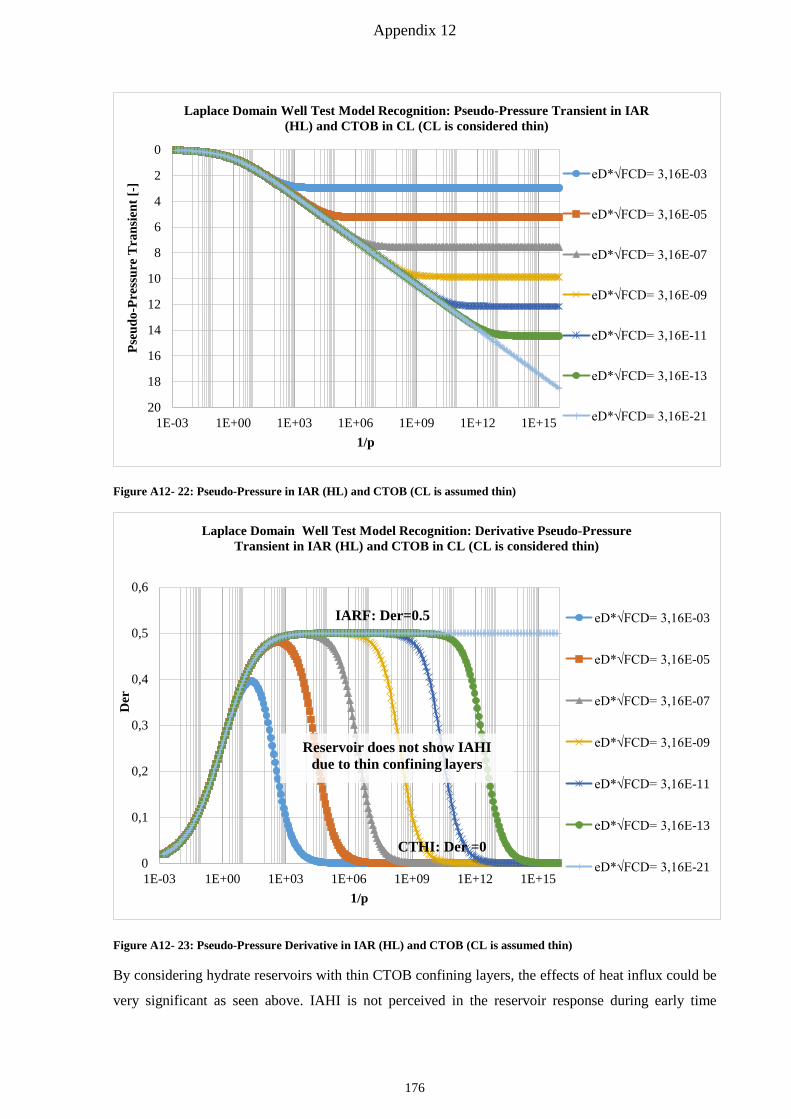
Appendix 12
Figure A12- 22: Pseudo-Pressure in IAR (HL) and CTOB (CL is assumed thin)
Figure A12- 23: Pseudo-Pressure Derivative in IAR (HL) and CTOB (CL is assumed thin)
By considering hydrate reservoirs with thin CTOB confining layers, the effects of heat influx could be
very significant as seen above. IAHI is not perceived in the reservoir response during early time
0
2
4
6
8
10
12
14
16
18
201E-03 1E+00 1E+03 1E+06 1E+09 1E+12 1E+15
Pseu
do-P
ress
ure
Tra
nsie
nt [-
]
1/p
Laplace Domain Well Test Model Recognition: Pseudo-Pressure Transient in IAR (HL) and CTOB in CL (CL is considered thin)
eD*√FCD= 3,16E-03
eD*√FCD= 3,16E-05
eD*√FCD= 3,16E-07
eD*√FCD= 3,16E-09
eD*√FCD= 3,16E-11
eD*√FCD= 3,16E-13
eD*√FCD= 3,16E-21
0
0,1
0,2
0,3
0,4
0,5
0,6
1E-03 1E+00 1E+03 1E+06 1E+09 1E+12 1E+15
Der
1/p
Laplace Domain Well Test Model Recognition: Derivative Pseudo-Pressure Transient in IAR (HL) and CTOB in CL (CL is considered thin)
eD*√FCD= 3,16E-03
eD*√FCD= 3,16E-05
eD*√FCD= 3,16E-07
eD*√FCD= 3,16E-09
eD*√FCD= 3,16E-11
eD*√FCD= 3,16E-13
eD*√FCD= 3,16E-21
IARF: Der=0.5
CTHI: Der =0
Reservoir does not show IAHI due to thin confining layers
176

Appendix 12
production phase which makes late time approximate solutions given by Hantush [43] applicable for
both the early and late time periods of production.
Figure A12- 24: Pseudo-Pressure in IAR (HL) and CTOB (CL is assumed thin)
Figure A12- 25: Pseudo-Pressure Derivative in IAR (HL) and p-NFTB in CL (CL is assumed very thick)
0
2
4
6
8
10
12
14
16
18
201E-03 1E+00 1E+03 1E+06 1E+09 1E+12 1E+15
Pseu
do-P
ress
ure
Tra
nsie
nt [-
]
1/p
Laplace Domain Well Test Model Recognition: Pseudo-Pressure Transient in IAR (HL) and p-NFTB in CL (CL is considered very thick)
eD*√FCD= 4,74E-01
eD*√FCD= 4,74E-02
eD*√FCD= 4,74E-03
eD*√FCD= 4,74E-04
eD*√FCD= 4,74E-05
eD*√FCD= 4,74E-06
eD*√FCD= 4,74E-14
0
0,1
0,2
0,3
0,4
0,5
0,6
1E-03 1E+00 1E+03 1E+06 1E+09 1E+12 1E+15
Der
1/p
Laplace Domain Well Test Model Recognition: Derivative Pseudo-Pressure Transient in IAR (HL) and p-NFTB in CL (CL is considered very thick)
eD*√FCD= 4,74E-01
eD*√FCD= 4,74E-02
eD*√FCD= 4,74E-03
eD*√FCD= 4,74E-04
eD*√FCD= 4,74E-05
eD*√FCD= 4,74E-06
eD*√FCD= 4,74E-14
PSSHI Dual Porosity Behavior as boundary of cofining layer is reached and heat influx
diminishes
IAHI: Der=0.25
IARF: Der =0.5
177
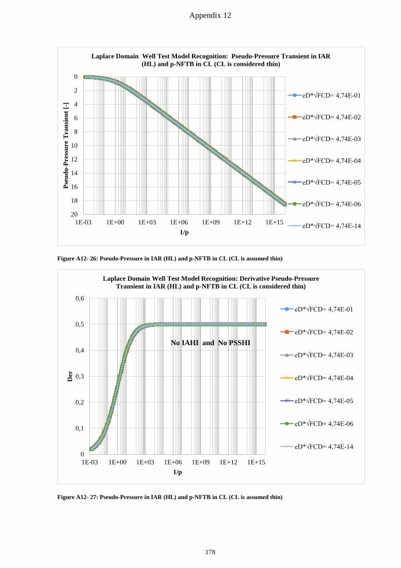
Appendix 12
Figure A12- 26: Pseudo-Pressure in IAR (HL) and p-NFTB in CL (CL is assumed thin)
Figure A12- 27: Pseudo-Pressure in IAR (HL) and p-NFTB in CL (CL is assumed thin)
0
2
4
6
8
10
12
14
16
18
201E-03 1E+00 1E+03 1E+06 1E+09 1E+12 1E+15
Pseu
do-P
ress
ure
Tra
nsie
nt [-
]
1/p
Laplace Domain Well Test Model Recognition: Pseudo-Pressure Transient in IAR (HL) and p-NFTB in CL (CL is considered thin)
eD*√FCD= 4,74E-01
eD*√FCD= 4,74E-02
eD*√FCD= 4,74E-03
eD*√FCD= 4,74E-04
eD*√FCD= 4,74E-05
eD*√FCD= 4,74E-06
eD*√FCD= 4,74E-14
0
0,1
0,2
0,3
0,4
0,5
0,6
1E-03 1E+00 1E+03 1E+06 1E+09 1E+12 1E+15
Der
1/p
Laplace Domain Well Test Model Recognition: Derivative Pseudo-Pressure Transient in IAR (HL) and p-NFTB in CL (CL is considered thin)
eD*√FCD= 4,74E-01
eD*√FCD= 4,74E-02
eD*√FCD= 4,74E-03
eD*√FCD= 4,74E-04
eD*√FCD= 4,74E-05
eD*√FCD= 4,74E-06
eD*√FCD= 4,74E-14
No IAHI and No PSSHI
178
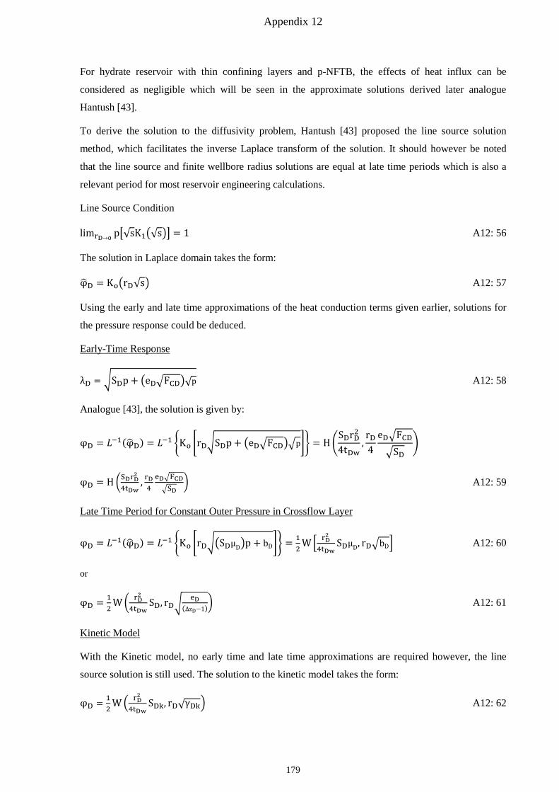
Appendix 12
For hydrate reservoir with thin confining layers and p-NFTB, the effects of heat influx can be
considered as negligible which will be seen in the approximate solutions derived later analogue
Hantush [43].
To derive the solution to the diffusivity problem, Hantush [43] proposed the line source solution
method, which facilitates the inverse Laplace transform of the solution. It should however be noted
that the line source and finite wellbore radius solutions are equal at late time periods which is also a
relevant period for most reservoir engineering calculations.
Line Source Condition
limrD→0 p�√sK1�√s�� = 1 A12: 56
The solution in Laplace domain takes the form:
φ�D = Ko�rD√s� A12: 57
Using the early and late time approximations of the heat conduction terms given earlier, solutions for
the pressure response could be deduced.
Early-Time Response
λD = �SDp + �eD�FCD�√p A12: 58
Analogue [43], the solution is given by:
φD = 𝐿𝐿−1(φ�D) = 𝐿𝐿−1 �Ko �rD�SDp + �eD�FCD��p�� = H�SDrD2
4tDw,rD4
eD�FCD�SD
�
φD = H �SDrD2
4tDw, rD4eD�FCD�SD
� A12: 59
Late Time Period for Constant Outer Pressure in Crossflow Layer
φD = 𝐿𝐿−1(φ�D) = 𝐿𝐿−1 �Ko �rD��SDµD�p + bD�� = 12
W � rD2
4tDwSDµD, rD�bD� A12: 60
or
φD = 12
W � rD2
4tDwSD, rD�
eD(∆zD−1)� A12: 61
Kinetic Model
With the Kinetic model, no early time and late time approximations are required however, the line
source solution is still used. The solution to the kinetic model takes the form:
φD = 12
W � rD2
4tDwSDk, rD√γDk� A12: 62
179
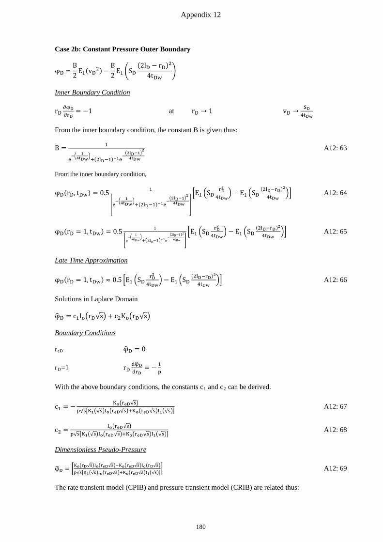
Appendix 12
Case 2b: Constant Pressure Outer Boundary
φD =B2
E1(vD2)−B2
E1 �SD(2lD − rD)2
4tDw�
Inner Boundary Condition
rD∂φD∂rD
= −1 at rD → 1 vD →SD4tDw
From the inner boundary condition, the constant B is given thus:
B = 1
e−� 1
4tDw�+(2lD−1)−1e
−�2lD−1�
2
4tDw
A12: 63
From the inner boundary condition,
φD(rD, tDw) = 0.5 1
�e−� 1
4tDw�+(2lD−1)−1e
−�2lD−1�
2
4tDw �
�E1 �SDrD2
4tDw� − E1 �SD
(2lD−rD)2
4tDw�� A12: 64
φD(rD = 1, tDw) = 0.5 1
�e−� 1
4tDw�
+(2lD−1)−1e−
(2lD−1)2
4tDw ��E1 �SD
rD2
4tDw� − E1 �SD
(2lD−rD)2
4tDw�� A12: 65
Late Time Approximation
φD(rD = 1, tDw) ≈ 0.5 �E1 �SDrD2
4tDw� − E1 �SD
(2lD−rD)2
4tDw�� A12: 66
Solutions in Laplace Domain
φ�D = c1Io�rD√s� + c2Ko�rD√s�
Boundary Conditions
reD φ�D = 0
rD=1 rDdφ�DdrD
= − 1p
With the above boundary conditions, the constants c1 and c2 can be derived.
c1 = − Ko�reD√s�p√s�K1�√s�Io�reD√s�+Ko�reD√s�I1�√s��
A12: 67
c2 = Io�reD√s�p√s�K1�√s�Io�reD√s�+Ko�reD√s�I1�√s��
A12: 68
Dimensionless Pseudo-Pressure
φ�D = �Ko�rD√s�Io�reD√s�−Ko�reD√s�Io�rD√s�p√s�K1�√s�Io�reD√s�+Ko�reD√s�I1�√s��
� A12: 69
The rate transient model (CPIB) and pressure transient model (CRIB) are related thus:
180

Appendix 12
pm� tD(rD = 1, p) = √s �K1�√s�Io�reD√s�+ Ko�reD√s�I1�√s�Io�reD√s�Ko�√s�−Io�√s�Ko�reD√s�
� =1
pφ�D
Pseudo-Pressure Transient Plot in Laplace Domain
φ�Dp Versus 1p
Der =∆(φ�Dp)
∆ �1p�
Versus 1p
For large values of p i.e. early time production period where boundary dominated flow has not been
reached, the reservoir is still acting infinite and from the characteristics of the modified Bessel´s
functions given in Figure A7- 1, the solutions to the infinite acting reservoir are applicable.
Figure A12- 28: Pseudo-Pressure in CPOB (HL) and IAR in CL
0
2
4
6
8
10
121E-03 1E+00 1E+03 1E+06 1E+09 1E+12
Pseu
do-P
ress
ure
Tra
nsie
nt [-
]
1/p
Laplace Domain Well Test Model Recognition: Pseudo-Pressure Transient in CPOB (HL) and IAR (CL) , (eD√FCD = 3.16E-03)
reD 250
reD 1250
reD 6250
reD ∞
181
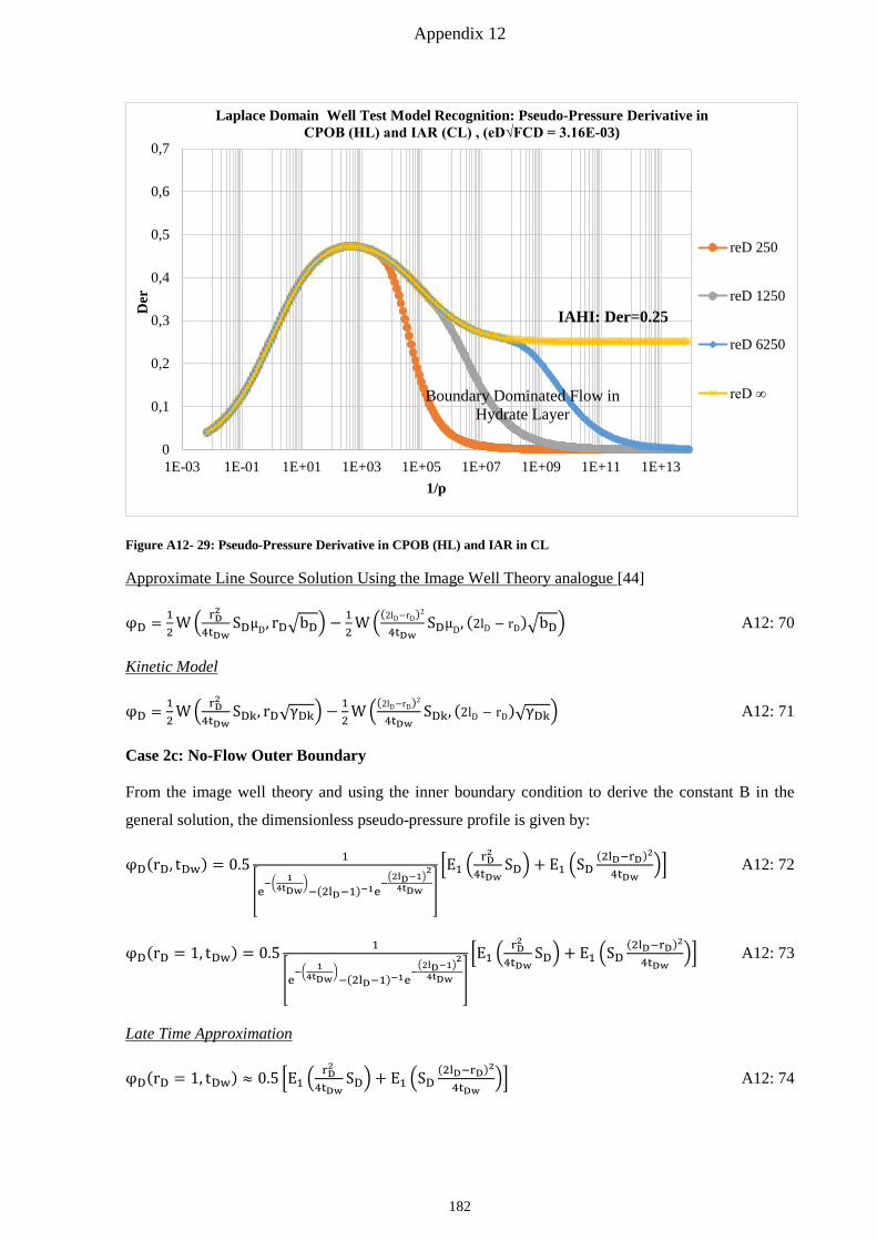
Appendix 12
Figure A12- 29: Pseudo-Pressure Derivative in CPOB (HL) and IAR in CL
Approximate Line Source Solution Using the Image Well Theory analogue [44]
φD = 12
W � rD2
4tDwSDµD, rD�bD� −
12
W �(2lD−rD)2
4tDwSDµD, (2lD − rD)�bD� A12: 70
Kinetic Model
φD = 12
W � rD2
4tDwSDk, rD√γDk� −
12
W �(2lD−rD)2
4tDwSDk, (2lD − rD)√γDk� A12: 71
Case 2c: No-Flow Outer Boundary
From the image well theory and using the inner boundary condition to derive the constant B in the
general solution, the dimensionless pseudo-pressure profile is given by:
φD(rD, tDw) = 0.5 1
�e−� 1
4tDw�−(2lD−1)−1e
−�2lD−1�
2
4tDw �
�E1 �rD2
4tDwSD� + E1 �SD
(2lD−rD)2
4tDw�� A12: 72
φD(rD = 1, tDw) = 0.5 1
�e−� 14tDw
�−(2lD−1)−1e
−�2lD−1�
2
4tDw �
�E1 �rD2
4tDwSD� + E1 �SD
(2lD−rD)2
4tDw�� A12: 73
Late Time Approximation
φD(rD = 1, tDw) ≈ 0.5 �E1 �rD2
4tDwSD�+ E1 �SD
(2lD−rD)2
4tDw�� A12: 74
0
0,1
0,2
0,3
0,4
0,5
0,6
0,7
1E-03 1E-01 1E+01 1E+03 1E+05 1E+07 1E+09 1E+11 1E+13
Der
1/p
Laplace Domain Well Test Model Recognition: Pseudo-Pressure Derivative in CPOB (HL) and IAR (CL) , (eD√FCD = 3.16E-03)
reD 250
reD 1250
reD 6250
reD ∞ Boundary Dominated Flow in Hydrate Layer
IAHI: Der=0.25
182
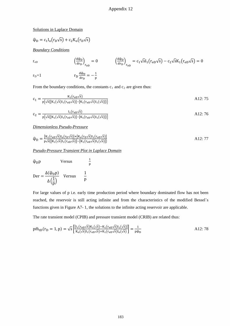
Appendix 12
Solutions in Laplace Domain
φ�D = c1Io�rD√s� + c2Ko�rD√s�
Boundary Conditions
reD �dφ�DdrD
�reD
= 0 �dφ�DdrD
�reD
= c1√sI1�reD√s� − c2√sK1�reD√s� = 0
rD=1 rDdφ�DdrD
= − 1p
From the boundary conditions, the constants c1 and c2 are given thus:
c1 = K1�reD√s�
p�√s��K1�√s�I1�reD√s��−�K1�reD√s�I1�√s���� A12: 75
c2 = I1�reD√s�
p�√s��K1�√s�I1�reD√s��−�K1�reD√s�I1�√s���� A12: 76
Dimensionless Pseudo-Pressure
φ�D = �K1�reD√s�Io�rD√s��+�Ko�rD√s�I1�reD√s��p√s��K1�√s�I1�reD√s��−�K1�reD√s�I1�√s���
A12: 77
Pseudo-Pressure Transient Plot in Laplace Domain
φ�Dp Versus 1p
Der =∆(φ�Dp)
∆ �1p�
Versus 1p
For large values of p i.e. early time production period where boundary dominated flow has not been
reached, the reservoir is still acting infinite and from the characteristics of the modified Bessel´s
functions given in Figure A7- 1, the solutions to the infinite acting reservoir are applicable.
The rate transient model (CPIB) and pressure transient model (CRIB) are related thus:
pm� tD(rD = 1, p) = √s ��I1�reD√s�K1�√s�−K1�reD√s�I1�√s��Ko�√s�I1�reD√s�+K1�reD√s�Io�√s�
� = 1pφ�D
A12: 78
183
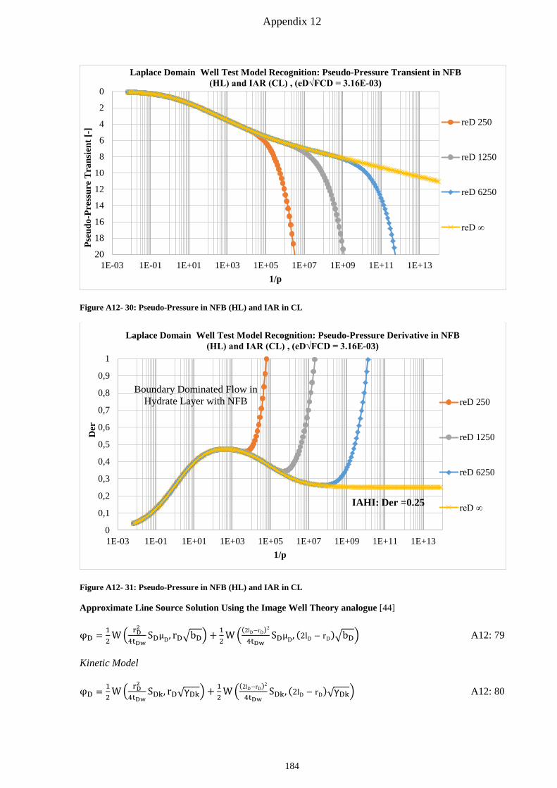
Appendix 12
Figure A12- 30: Pseudo-Pressure in NFB (HL) and IAR in CL
Figure A12- 31: Pseudo-Pressure in NFB (HL) and IAR in CL
Approximate Line Source Solution Using the Image Well Theory analogue [44]
φD = 12
W � rD2
4tDwSDµD, rD�bD� + 1
2W �(2lD−rD)2
4tDwSDµD, (2lD − rD)�bD� A12: 79
Kinetic Model
φD = 12
W � rD2
4tDwSDk, rD√γDk� + 1
2W �(2lD−rD)2
4tDwSDk, (2lD − rD)√γDk� A12: 80
0
2
4
6
8
10
12
14
16
18
201E-03 1E-01 1E+01 1E+03 1E+05 1E+07 1E+09 1E+11 1E+13
Pseu
do-P
ress
ure
Tra
nsie
nt [-
]
1/p
Laplace Domain Well Test Model Recognition: Pseudo-Pressure Transient in NFB (HL) and IAR (CL) , (eD√FCD = 3.16E-03)
reD 250
reD 1250
reD 6250
reD ∞
0
0,1
0,2
0,3
0,4
0,5
0,6
0,7
0,8
0,9
1
1E-03 1E-01 1E+01 1E+03 1E+05 1E+07 1E+09 1E+11 1E+13
Der
1/p
Laplace Domain Well Test Model Recognition: Pseudo-Pressure Derivative in NFB (HL) and IAR (CL) , (eD√FCD = 3.16E-03)
reD 250
reD 1250
reD 6250
reD ∞ IAHI: Der =0.25
Boundary Dominated Flow in Hydrate Layer with NFB
184
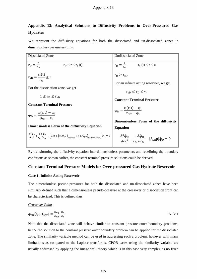
Appendix 13
Appendix 13: Analytical Solutions to Diffusivity Problems in Over-Pressured Gas
Hydrates
We represent the diffusivity equations for both the dissociated and un-dissociated zones in
dimensionless parameters thus:
Dissociated Zone Undissociated Zone
rD = rrw
rw ≤ r ≤ rs (t)
rsD =rs(t)
rw≥ 1
For the dissociation zone, we get
1 ≤ rD ≤ rsD
Constant Terminal Pressure
φD =φ(r, t) − φiφwf − φi
Dimensionless Form of the diffusivity Equation
∂2φ�D∂rD2
+1rD∂φ�D ∂rD
− �SDp + �eDQpD� �
𝐶𝐶𝐶𝐶𝐶𝐶𝐶𝐶𝐶𝐶𝐶𝐶𝑘𝑘+ �eDQpD
� �𝑈𝑈𝑈𝑈𝑈𝑈𝑈𝑈𝐶𝐶𝑈𝑈𝑈𝑈𝐶𝐶𝑈𝑈𝑈𝑈𝑈𝑈
�φ�D = 0
rD = rrw
rs (t) ≤ r ≤ ∞
rD ≥ rsD
For an infinite acting reservoir, we get
rsD ≤ rD ≤ ∞
Constant Terminal Pressure
φD =φ(r, t) − φiφwf − φi
Dimensionless Form of the diffusivity
Equation
∂2φ�D∂rD2
+1rD∂φ�D ∂rD
− [SDkp]φ�D = 0
By transforming the diffusivity equation into dimensionless parameters and redefining the boundary
conditions as shown earlier, the constant terminal pressure solutions could be derived.
Constant Terminal Pressure Models for Over-pressured Gas Hydrate Reservoir
Case 1: Infinite Acting Reservoir
The dimensionless pseudo-pressures for both the dissociated and un-dissociated zones have been
similarly defined such that a dimensionless pseudo-pressure at the crossover or dissociation front can
be characterized. This is defined thus:
Crossover Point
φsD(rsD, tDw) = φeq−φi
φwf−φi A13: 1
Note that the dissociated zone will behave similar to constant pressure outer boundary problems;
hence the solution to the constant pressure outer boundary problem can be applied for the dissociated
zone. The similarity variable method can be used in addressing such a problem; however with many
limitations as compared to the Laplace transforms. CPOB cases using the similarity variable are
usually addressed by applying the image well theory which is in this case very complex as no fixed
185
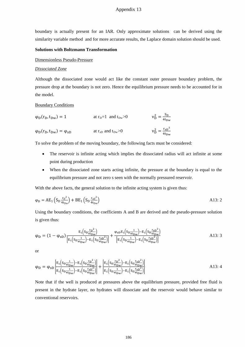
Appendix 13
boundary is actually present for an IAR. Only approximate solutions can be derived using the
similarity variable method and for more accurate results, the Laplace domain solution should be used.
Solutions with Boltzmann Transformation
Dimensionless Pseudo-Pressure
Dissociated Zone
Although the dissociated zone would act like the constant outer pressure boundary problem, the
pressure drop at the boundary is not zero. Hence the equilibrium pressure needs to be accounted for in
the model.
Boundary Conditions
φD(rD, tDw) = 1 at rD=1 and tDw>0 vD2 = SD4tDw
φD(rD, tDw) = φsD at rsD and tDw>0 vD2 = rsD2
4tDw
To solve the problem of the moving boundary, the following facts must be considered:
• The reservoir is infinite acting which implies the dissociated radius will act infinite at some
point during production
• When the dissociated zone starts acting infinite, the pressure at the boundary is equal to the
equilibrium pressure and not zero s seen with the normally pressured reservoir.
With the above facts, the general solution to the infinite acting system is given thus:
φD = AE1 �SDrD2
4tDw� + BE1 �SD
rsD2
4tDw� A13: 2
Using the boundary conditions, the coefficients A and B are derived and the pseudo-pressure solution
is given thus:
φD = (1 − φsD)E1�SD
rD2
4tDw�
�E1�SD1
4tDw�−E1�SD
rsD2
4tDw��
+φsDE1�SD
14tDw
�−E1�SDrsD
2
4tDw�
�E1�SD1
4tDw�−E1�SD
rsD2
4tDw��
A13: 3
or
φD = φsD�E1�SD
14tDw
�−E1�SDrD2
4tDw��
�E1�SD1
4tDw�−E1�SD
rsD2
4tDw��
+�E1�SD
rD2
4tDw�−E1�SD
rsD2
4tDw��
�E1�SD1
4tDw�−E1�SD
rsD2
4tDw��
A13: 4
Note that if the well is produced at pressures above the equilibrium pressure, provided free fluid is
present in the hydrate layer, no hydrates will dissociate and the reservoir would behave similar to
conventional reservoirs.
186

Appendix 13
The solution to the problem takes the form:
Pwf ≥ Peq
φD =E1�SDk
rD2
4tDw�
E1�SDk4tDw
� A13: 5
The moving boundary model proposed by [70] and [72] considered the reservoir pressure in the
dissociated zone to be equal to the equilibrium pressure, making the dimensionless equilibrium
pressure equal zero at the dissociation front and their model can be represented in terms of pseudo-
pressure thus [70], [72]:
φD = φ(r,t)−φeq
φwf−φeq=
�E1�SDrD2
4tDw�−E1�SD
rsD2
4tDw��
�E1�SD1
4tDw�−E1�SD
rsD2
4tDw��
A13: 6
Radius of Dissociation
The definition of the radius of dissociation has been a challenge for many analytical models for the
moving boundary problem. Most models used in deriving the transient radius of dissociation are based
on the model proposed by [71], which simply addresses mass balance at the dissociation front.
In a similar manner, we address the following boundary conditions at the dissociation front:
[φD]dissociation front = φsD A13: 7
[mtD] front(dissociated zone) = [mtD] front(undissociated zone) A13: 8
Efforts will now be made to derive the solutions for the rate transient at the fronts.
Rate Transient
Dissociated Zone
mtD = −rDdφD∂rD
From the deduced pressure profile in the dissociated zone, we get:
mtD = (1 − φsD) 2e−�
rD24tDw
SD�
�E1�SD1
4tDw�−E1�SD
rsD2
4tDw��
A13: 9
Pwf ≥ Peq
mtD = 2
�E1�SDk4tDw
��e−�SDk
rD2
4tDw� A13: 10
Undissociated Zone
φD = B �E1 �rD2
4tDwSDk�� A13: 11
187

Appendix 13
Unlike methods seen earlier in deducing the constant B in the above equation, here, the constant has to
be derived based on the boundary conditions at the dissociation front and the outer boundary of the
undissociated zone.
We now apply the first boundary condition at the crossover point such that the constant B is obtained.
φD = φsD
�E1�rD2
4tDwSDk��
�E1�rsD24tDw
SDk�� A13: 12
The mass rate at the dissociation front obtained front the solution of the undissociated region is given
by:
mtD = 2φsD
�E1�rsD2
4tDwSDk��
e−�
rD2
4tDwSDk�
A13: 13
By equating the solutions for the dimensionless mass rates for each zone we get the following
relationship which must always be satisfied.
mtD = 2φsD
�E1�rsD2
4tDwSDk��
e−�
rsD2
4tDwSDk�
= (1 − φsD) 2e−�
rsD24tDw
SD�
�E1�SD1
4tDw�−E1�SD
rsD2
4tDw��
A13: 14
Criterion for Valid Radius of Dissociation
2φsD
�E1�rsD24tDw
SDk��e−�
rsD2
4tDwSDk� = �1−φsD�
2e−�
rsD24tDw
SD�
�E1�SD1
4tDw�−E1�SD
rsD24tDw
�� A13: 15
For a given value of φsD, tDw and SDk/SD, the above equation should be computed for arbitrary values
of rsD till the criterion is fulfilled. For all boundary conditions to be valid, the above criterion must be
obeyed at all times. Note that if φsD=0, the transient rate solution for the dissociated zone reduces to
the solution for the normally pressured gas hydrates as rsD→∞.
Solution in Laplace Domain
The solutions in Laplace domain give the exact solution to the problem.
Dimensionless Pseudo-Pressure
Dissociated Zone
φ�D = c1Io�rD√s� + c2Ko�rD√s�
Boundary Conditions
rsD φ�D = φsDp
rD=1 φ�D = 1p
188
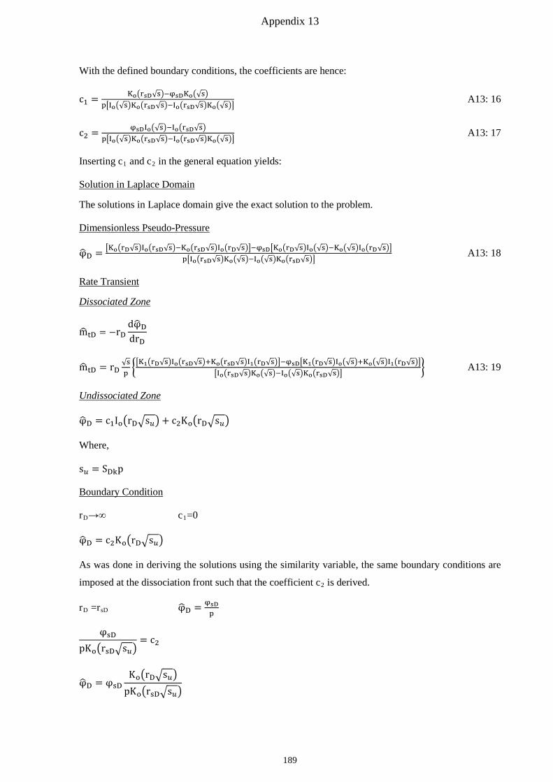
Appendix 13
With the defined boundary conditions, the coefficients are hence:
c1 = Ko�rsD√s�−φsDKo�√s�p�Io�√s�Ko�rsD√s�−Io�rsD√s�Ko�√s��
A13: 16
c2 = φsDIo�√s�−Io�rsD√s�p�Io�√s�Ko�rsD√s�−Io�rsD√s�Ko�√s��
A13: 17
Inserting c1 and c2 in the general equation yields:
Solution in Laplace Domain
The solutions in Laplace domain give the exact solution to the problem.
Dimensionless Pseudo-Pressure
φ�D = �Ko�rD√s�Io�rsD√s�−Ko�rsD√s�Io�rD√s��−φsD�Ko�rD√s�Io�√s�−Ko�√s�Io�rD√s��p�Io�rsD√s�Ko�√s�−Io�√s�Ko�rsD√s��
A13: 18
Rate Transient
Dissociated Zone
m� tD = −rDdφ�DdrD
m� tD = rD√sp��K1�rD√s�Io�rsD√s�+Ko�rsD√s�I1�rD√s��−φsD�K1�rD√s�Io�√s�+Ko�√s�I1�rD√s��
�Io�rsD√s�Ko�√s�−Io�√s�Ko�rsD√s��� A13: 19
Undissociated Zone
φ�D = c1Io�rD�s𝑈𝑈� + c2Ko�rD�s𝑈𝑈�
Where,
s𝑈𝑈 = SDkp
Boundary Condition
rD→∞ c1=0
φ�D = c2Ko�rD�s𝑈𝑈�
As was done in deriving the solutions using the similarity variable, the same boundary conditions are
imposed at the dissociation front such that the coefficient c2 is derived.
rD =rsD φ�D = φsDp
φsDpKo�rsD�s𝑈𝑈�
= c2
φ�D = φsDKo�rD�s𝑈𝑈�
pKo�rsD�s𝑈𝑈�
189
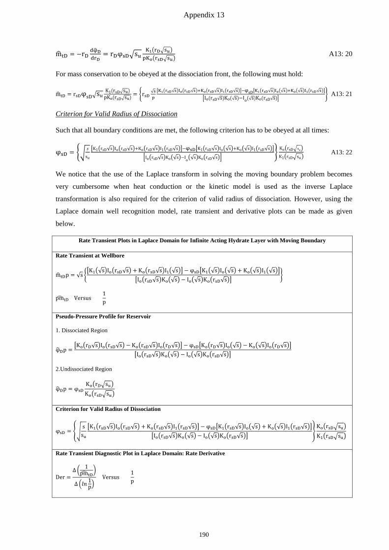
Appendix 13
m� tD = −rDdφ�DdrD
= rDφsD�s𝑈𝑈K1�rD�s𝑢𝑢�pKo�rsD�s𝑢𝑢�
A13: 20
For mass conservation to be obeyed at the dissociation front, the following must hold:
m�tD = rsDφsD�s𝑉𝑉K1�rsD�s𝑉𝑉�
pKo�rsD�s𝑉𝑉�= �rsD
√sp�K1�rsD√s�Io�rsD√s�+Ko�rsD√s�I1�rsD√s��−φsD�K1�rsD√s�Io�√s�+Ko�√s�I1�rsD√s��
�Io�rsD√s�Ko�√s�−Io�√s�Ko�rsD√s��� A13: 21
Criterion for Valid Radius of Dissociation
Such that all boundary conditions are met, the following criterion has to be obeyed at all times:
φsD = ��𝑉𝑉
s𝑉𝑉
�K1�rsD√s�Io�rsD√s�+Ko�rsD√s�I1�rsD√s��−φsD�K1�rsD√s�Io�√s�+Ko�√s�I1�rsD√s��
�Io�rsD√s�Ko�√s�−Io�√s�Ko�rsD√s��� Ko�rsD�s𝑉𝑉�
K1�rsD�s𝑉𝑉� A13: 22
We notice that the use of the Laplace transform in solving the moving boundary problem becomes
very cumbersome when heat conduction or the kinetic model is used as the inverse Laplace
transformation is also required for the criterion of valid radius of dissociation. However, using the
Laplace domain well recognition model, rate transient and derivative plots can be made as given
below.
Rate Transient Plots in Laplace Domain for Infinite Acting Hydrate Layer with Moving Boundary
Rate Transient at Wellbore
m�tDp = √s ��K1�√s�Io�rsD√s� + Ko�rsD√s�I1�√s�� − φsD�K1�√s�Io�√s� + Ko�√s�I1�√s��
�Io�rsD√s�Ko�√s� − Io�√s�Ko�rsD√s���
pm� tD Versus 1p
Pseudo-Pressure Profile for Reservoir
1. Dissociated Region
φ�Dp =�Ko�rD√s�Io�rsD√s� − Ko�rsD√s�Io�rD√s�� − φsD�Ko�rD√s�Io�√s� − Ko�√s�Io�rD√s��
�Io�rsD√s�Ko�√s� − Io�√s�Ko�rsD√s��
2.Undissociated Region
φ�Dp = φsDKo�rD�s𝑈𝑈�Ko�rsD�s𝑈𝑈�
Criterion for Valid Radius of Dissociation
φsD = ��s
su�K1�rsD√s�Io�rsD√s� + Ko�rsD√s�I1�rsD√s�� − φsD�K1�rsD√s�Io�√s� + Ko�√s�I1�rsD√s��
�Io�rsD√s�Ko�√s� − Io�√s�Ko�rsD√s���
Ko�rsD�su�K1�rsD�su�
Rate Transient Diagnostic Plot in Laplace Domain: Rate Derivative
Der =∆ � 1
pm� tD�
∆ �𝑙𝑙𝑙𝑙 1p�
Versus 1p
190
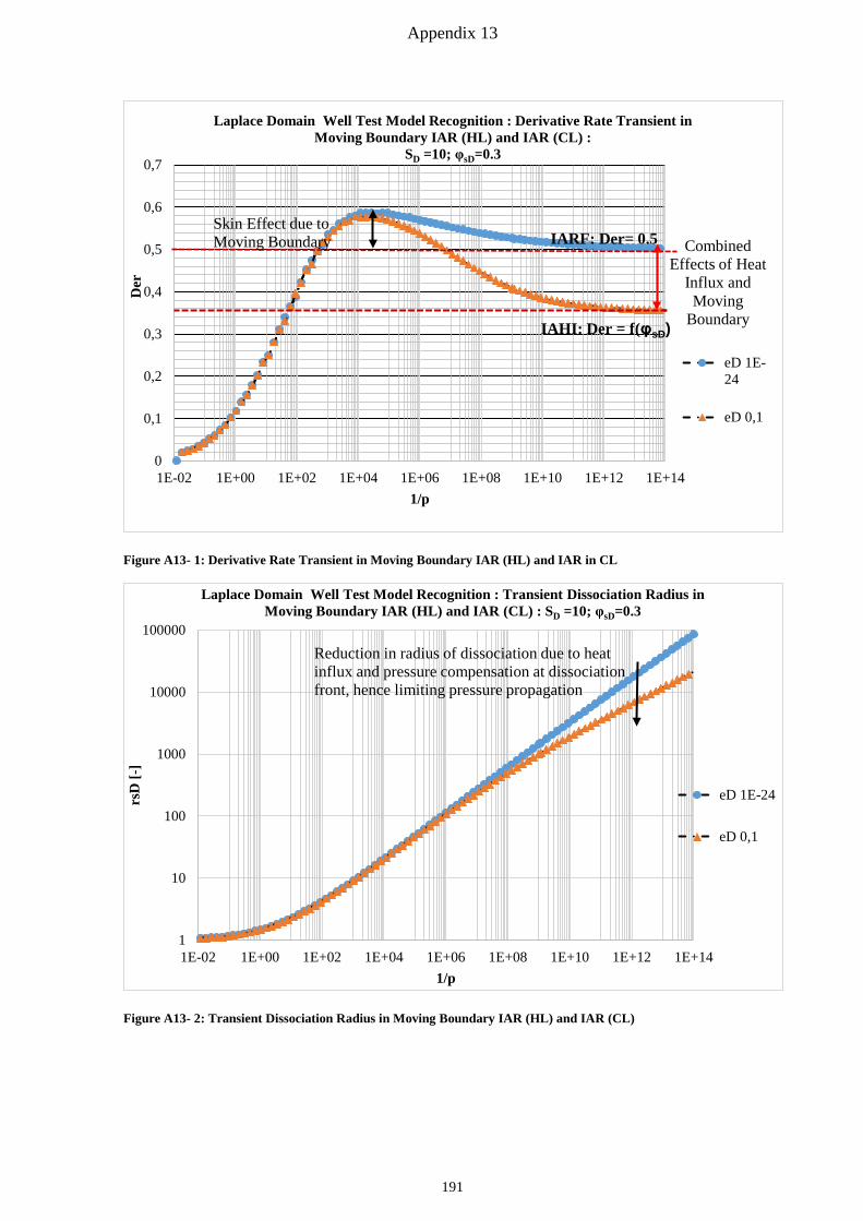
Appendix 13
Figure A13- 1: Derivative Rate Transient in Moving Boundary IAR (HL) and IAR in CL
Figure A13- 2: Transient Dissociation Radius in Moving Boundary IAR (HL) and IAR (CL)
0
0,1
0,2
0,3
0,4
0,5
0,6
0,7
1E-02 1E+00 1E+02 1E+04 1E+06 1E+08 1E+10 1E+12 1E+14
Der
1/p
Laplace Domain Well Test Model Recognition : Derivative Rate Transient in Moving Boundary IAR (HL) and IAR (CL) :
SD =10; φsD=0.3
eD 1E-24
eD 0,1
IAHI: Der = f(φsD)
IARF: Der= 0.5 Skin Effect due to Moving Boundary Combined
Effects of Heat Influx and Moving
Boundary
1
10
100
1000
10000
100000
1E-02 1E+00 1E+02 1E+04 1E+06 1E+08 1E+10 1E+12 1E+14
rsD
[-]
1/p
Laplace Domain Well Test Model Recognition : Transient Dissociation Radius in Moving Boundary IAR (HL) and IAR (CL) : SD =10; φsD=0.3
eD 1E-24
eD 0,1
Reduction in radius of dissociation due to heat influx and pressure compensation at dissociation front, hence limiting pressure propagation
191

Appendix 13
Figure A13- 3: Derivative Rate Transient in Moving Boundary IAR (HL) and IAR in CL with insignificant Heat flux
Figure A13- 4: Derivative Rate Transient in Moving Boundary IAR (HL) and IAR in CL with insignificant Heat flux
0
0,1
0,2
0,3
0,4
0,5
0,6
0,7
1E-03 1E-02 1E-01 1E+00 1E+01 1E+02 1E+03 1E+04 1E+05 1E+06
Der
1/(pSD)
Laplace Domain Well Test Model Recognition : Derivative Rate Transient in Moving Boundary IAR (HL) and IAR (CL) : eD =1.00E-24
SD 10
SD 500
Increasing Skin with Increasing SD
0
0,1
0,2
0,3
0,4
0,5
0,6
0,7
0,8
0,9
0,01 1 100 10000 1000000 100000000 1E+10
Der
1/p
Laplace Domain Well Test Model Recognition : Derivative Rate Transient in Moving Boundary IAR (HL) with Zero Heat Influx and Influence of Equilibrium
Pressure: SD=10
ΨsD 0
ΨsD 0,3
ΨsD 0,5
ΨsD 0,7
ΨsD 0,9 Derivatives show dual porosity behavior due to limited radius of dissociation and low equilibrium
pressure
No Dual Porosity Behavior perceptible for 0.5*Pi<Peq< Pi
Increasing skin with decreasing equilibrium pressure
IARF: Der = 0.5
192
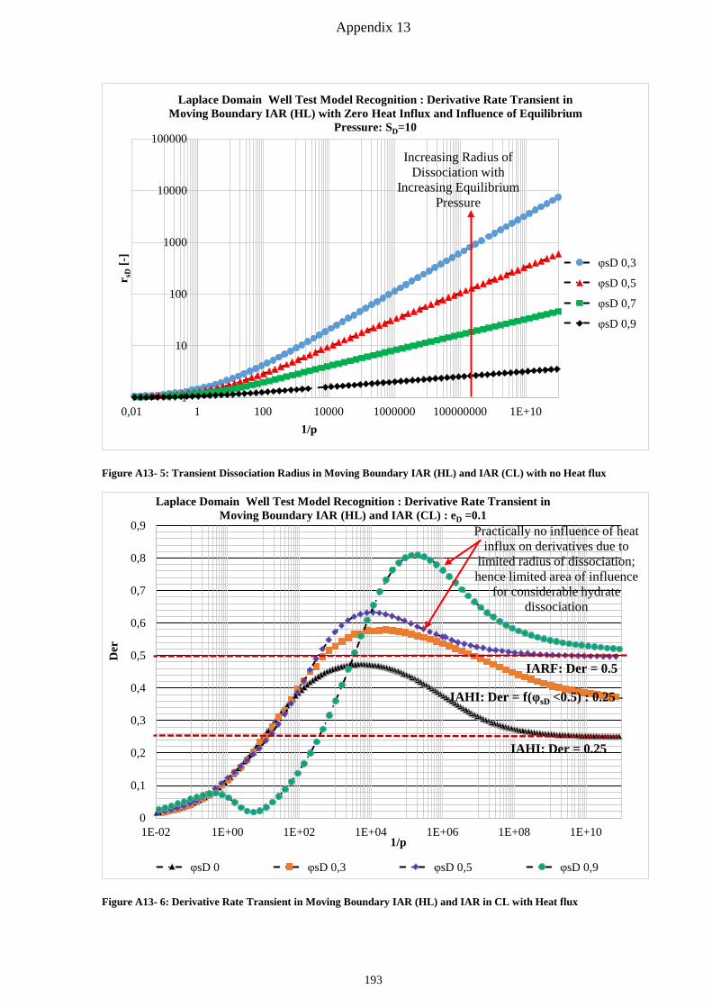
Appendix 13
Figure A13- 5: Transient Dissociation Radius in Moving Boundary IAR (HL) and IAR (CL) with no Heat flux
Figure A13- 6: Derivative Rate Transient in Moving Boundary IAR (HL) and IAR in CL with Heat flux
1
10
100
1000
10000
100000
0,01 1 100 10000 1000000 100000000 1E+10
r sD [-
]
1/p
Laplace Domain Well Test Model Recognition : Derivative Rate Transient in Moving Boundary IAR (HL) with Zero Heat Influx and Influence of Equilibrium
Pressure: SD=10
φsD 0,3
φsD 0,5
φsD 0,7
φsD 0,9
Increasing Radius of Dissociation with
Increasing Equilibrium Pressure
0
0,1
0,2
0,3
0,4
0,5
0,6
0,7
0,8
0,9
1E-02 1E+00 1E+02 1E+04 1E+06 1E+08 1E+10
Der
1/p
Laplace Domain Well Test Model Recognition : Derivative Rate Transient in Moving Boundary IAR (HL) and IAR (CL) : eD =0.1
φsD 0 φsD 0,3 φsD 0,5 φsD 0,9
Practically no influence of heat influx on derivatives due to
limited radius of dissociation; hence limited area of influence
for considerable hydrate dissociation
IAHI: Der = 0.25
IAHI: Der = f(φsD <0.5) : 0.25 -
IARF: Der = 0.5
193
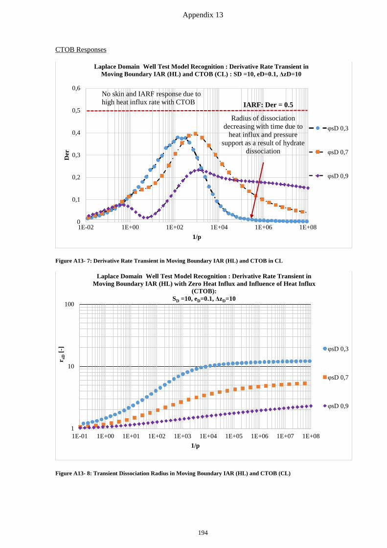
Appendix 13
CTOB Responses
Figure A13- 7: Derivative Rate Transient in Moving Boundary IAR (HL) and CTOB in CL
Figure A13- 8: Transient Dissociation Radius in Moving Boundary IAR (HL) and CTOB (CL)
0
0,1
0,2
0,3
0,4
0,5
0,6
1E-02 1E+00 1E+02 1E+04 1E+06 1E+08
Der
1/p
Laplace Domain Well Test Model Recognition : Derivative Rate Transient in Moving Boundary IAR (HL) and CTOB (CL) : SD =10, eD=0.1, ΔzD=10
φsD 0,3
φsD 0,7
φsD 0,9
IARF: Der = 0.5
Radius of dissociation decreasing with time due to
heat influx and pressure support as a result of hydrate
dissociation
No skin and IARF response due to high heat influx rate with CTOB
1
10
100
1E-01 1E+00 1E+01 1E+02 1E+03 1E+04 1E+05 1E+06 1E+07 1E+08
r sD [-
]
1/p
Laplace Domain Well Test Model Recognition : Derivative Rate Transient in Moving Boundary IAR (HL) with Zero Heat Influx and Influence of Heat Influx
(CTOB): SD =10, eD=0.1, ΔzD=10
φsD 0,3
φsD 0,7
φsD 0,9
194
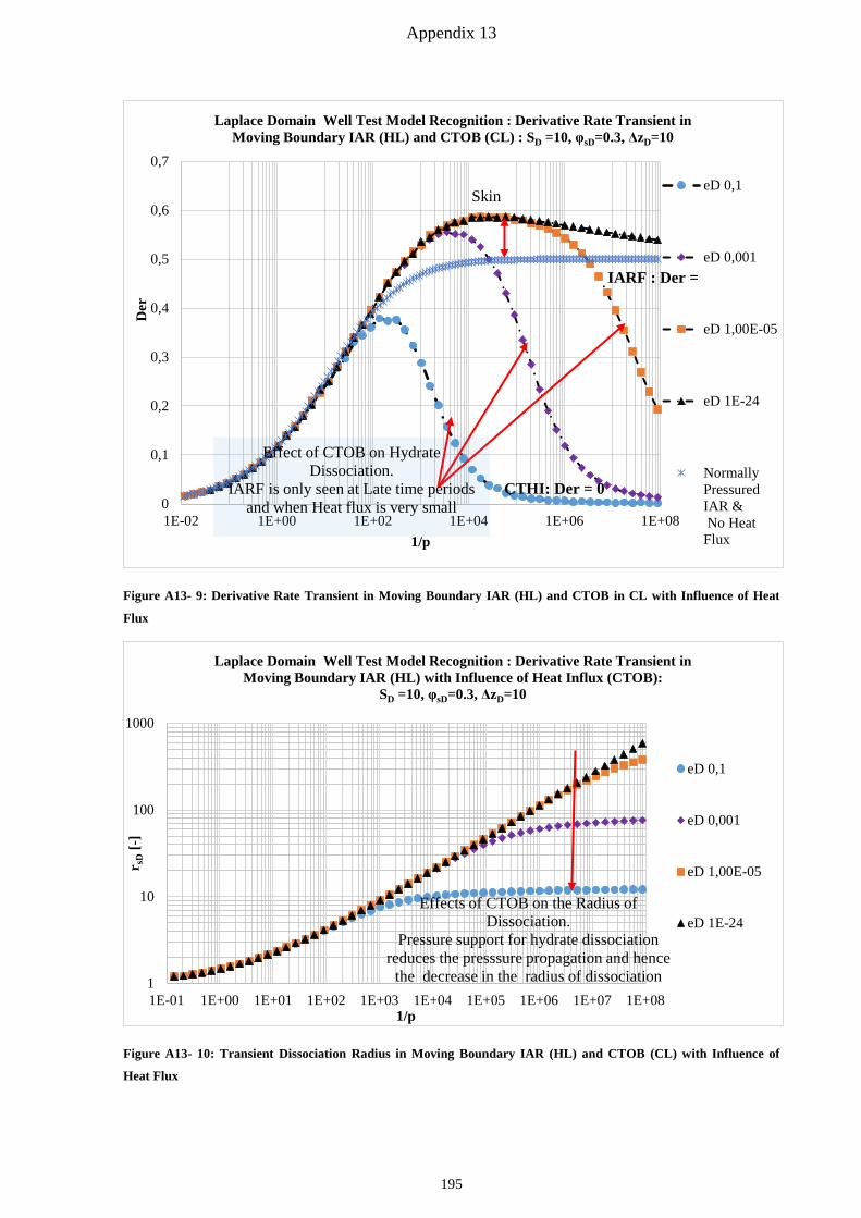
Appendix 13
Figure A13- 9: Derivative Rate Transient in Moving Boundary IAR (HL) and CTOB in CL with Influence of Heat
Flux
Figure A13- 10: Transient Dissociation Radius in Moving Boundary IAR (HL) and CTOB (CL) with Influence of
Heat Flux
0
0,1
0,2
0,3
0,4
0,5
0,6
0,7
1E-02 1E+00 1E+02 1E+04 1E+06 1E+08
Der
1/p
Laplace Domain Well Test Model Recognition : Derivative Rate Transient in Moving Boundary IAR (HL) and CTOB (CL) : SD =10, φsD=0.3, ΔzD=10
eD 0,1
eD 0,001
eD 1,00E-05
eD 1E-24
NormallyPressuredIAR & No HeatFlux
IARF : Der =
Skin
CTHI: Der = 0
Effect of CTOB on Hydrate Dissociation.
IARF is only seen at Late time periods and when Heat flux is very small
1
10
100
1000
1E-01 1E+00 1E+01 1E+02 1E+03 1E+04 1E+05 1E+06 1E+07 1E+08
r sD [-
]
1/p
Laplace Domain Well Test Model Recognition : Derivative Rate Transient in Moving Boundary IAR (HL) with Influence of Heat Influx (CTOB):
SD =10, φsD=0.3, ΔzD=10
eD 0,1
eD 0,001
eD 1,00E-05
eD 1E-24Effects of CTOB on the Radius of
Dissociation. Pressure support for hydrate dissociation
reduces the presssure propagation and hence the decrease in the radius of dissociation
195
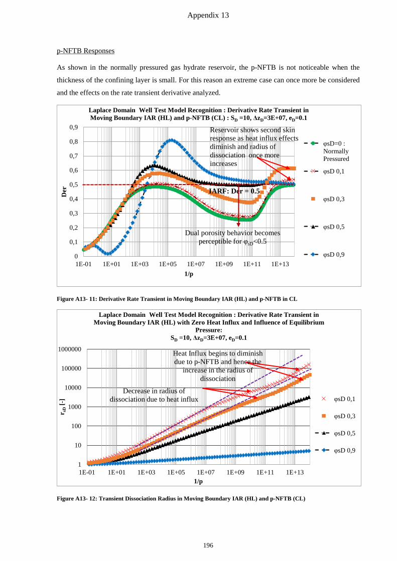
Appendix 13
p-NFTB Responses
As shown in the normally pressured gas hydrate reservoir, the p-NFTB is not noticeable when the
thickness of the confining layer is small. For this reason an extreme case can once more be considered
and the effects on the rate transient derivative analyzed.
Figure A13- 11: Derivative Rate Transient in Moving Boundary IAR (HL) and p-NFTB in CL
Figure A13- 12: Transient Dissociation Radius in Moving Boundary IAR (HL) and p-NFTB (CL)
0
0,1
0,2
0,3
0,4
0,5
0,6
0,7
0,8
0,9
1E-01 1E+01 1E+03 1E+05 1E+07 1E+09 1E+11 1E+13
Der
1/p
Laplace Domain Well Test Model Recognition : Derivative Rate Transient in Moving Boundary IAR (HL) and p-NFTB (CL) : SD =10, ΔzD=3E+07, eD=0.1
φsD=0 : Normally Pressured
φsD 0,1
φsD 0,3
φsD 0,5
φsD 0,9
IARF: Der = 0.5
Dual porosity behavior becomes perceptible for φsD<0.5
Reservoir shows second skin response as heat influx effects diminish and radius of dissociation once more increases
1
10
100
1000
10000
100000
1000000
1E-01 1E+01 1E+03 1E+05 1E+07 1E+09 1E+11 1E+13
r sD [-
]
1/p
Laplace Domain Well Test Model Recognition : Derivative Rate Transient in Moving Boundary IAR (HL) with Zero Heat Influx and Influence of Equilibrium
Pressure: SD =10, ΔzD=3E+07, eD=0.1
φsD 0,1
φsD 0,3
φsD 0,5
φsD 0,9
Heat Influx begins to diminish due to p-NFTB and hence the
increase in the radius of dissociation
Decrease in radius of dissociation due to heat influx
196
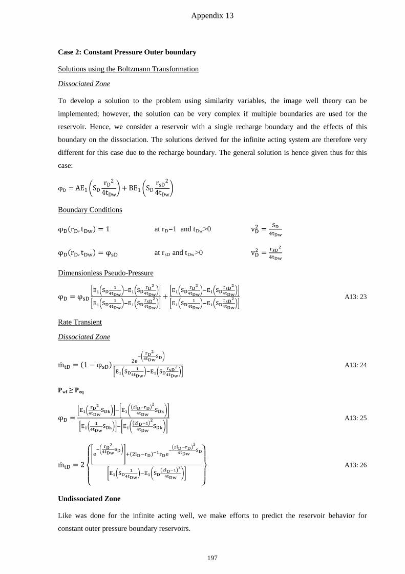
Appendix 13
Case 2: Constant Pressure Outer boundary
Solutions using the Boltzmann Transformation
Dissociated Zone
To develop a solution to the problem using similarity variables, the image well theory can be
implemented; however, the solution can be very complex if multiple boundaries are used for the
reservoir. Hence, we consider a reservoir with a single recharge boundary and the effects of this
boundary on the dissociation. The solutions derived for the infinite acting system are therefore very
different for this case due to the recharge boundary. The general solution is hence given thus for this
case:
φD = AE1 �SDrD
2
4tDw� + BE1 �SD
rsD2
4tDw�
Boundary Conditions
φD(rD, tDw) = 1 at rD=1 and tDw>0 vD2 = SD4tDw
φD(rD, tDw) = φsD at rsD and tDw>0 vD2 = rsD2
4tDw
Dimensionless Pseudo-Pressure
φD = φsD�E1�SD
14tDw
�−E1�SDrD2
4tDw��
�E1�SD1
4tDw�−E1�SD
rsD2
4tDw��
+�E1�SD
rD2
4tDw�−E1�SD
rsD2
4tDw��
�E1�SD1
4tDw�−E1�SD
rsD2
4tDw��
A13: 23
Rate Transient
Dissociated Zone
mtD = (1 − φsD) 2e−�
rD24tDw
SD�
�E1�SD1
4tDw�−E1�SD
rsD2
4tDw��
A13: 24
Pwf ≥ Peq
φD =�E1�
rD2
4tDwSDk��−�E1�
�2lD−rD�2
4tDwSDk��
�E1�1
4tDwSDk��−�E1�
�2lD−1�2
4tDwSDk��
A13: 25
mtD = 2
⎩⎪⎨
⎪⎧�e
−�rD
24tDw
SD��+(2lD−rD)−1rDe
−�2lD−rD�
2
4tDwSD
�E1�SD1
4tDw�−E1�SD
�2lD−1�2
4tDw��
⎭⎪⎬
⎪⎫
A13: 26
Undissociated Zone
Like was done for the infinite acting well, we make efforts to predict the reservoir behavior for
constant outer pressure boundary reservoirs.
197
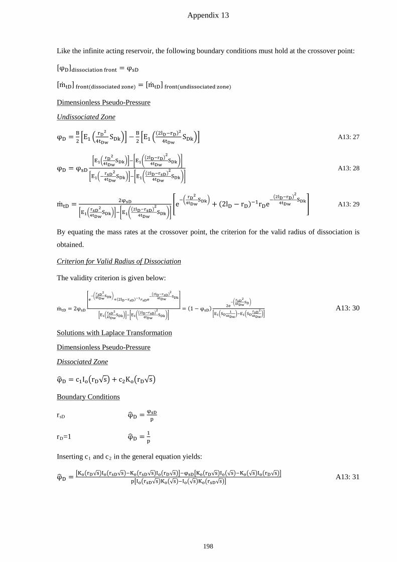
Appendix 13
Like the infinite acting reservoir, the following boundary conditions must hold at the crossover point:
[φD]dissociation front = φsD
[mtD] front(dissociated zone) = [mtD] front(undissociated zone)
Dimensionless Pseudo-Pressure
Undissociated Zone
φD = B2�E1 �
rD2
4tDwSDk�� −
B2�E1 �
(2lD−rD)2
4tDwSDk�� A13: 27
φD = φsD�E1�
rD2
4tDwSDk��−�E1�
�2lD−rD�2
4tDwSDk��
�E1�−rsD2
4tDwSDk��−�E1�
�2lD−rsD�2
4tDwSDk��
A13: 28
mtD = 2φsD
�E1�rsD2
4tDwSDk��−�E1�
�2lD−rsD�2
4tDwSDk��
�e−� rD2
4tDwSDk� + (2lD − rD)−1rDe−
�2lD−rD�2
4tDwSDk� A13: 29
By equating the mass rates at the crossover point, the criterion for the valid radius of dissociation is
obtained.
Criterion for Valid Radius of Dissociation
The validity criterion is given below:
mtD = 2φsD
�e−�𝑟𝑟sD
24tDw
SDk�+(2lD−rsD)−1𝐶𝐶sDe−�2lD−𝑟𝑟sD�
2
4tDwSDk�
�E1�rsD24tDw
SDk��−�E1��2lD−𝑟𝑟sD�
2
4tDwSDk��
= (1 − φsD) 2e−�
rsD24tDw
SD�
�E1�SD1
4tDw�−E1�SD
rsD2
4tDw�� A13: 30
Solutions with Laplace Transformation
Dimensionless Pseudo-Pressure
Dissociated Zone
φ�D = c1Io�rD√s� + c2Ko�rD√s�
Boundary Conditions
rsD φ�D = φsDp
rD=1 φ�D = 1p
Inserting c1 and c2 in the general equation yields:
φ�D = �Ko�rD√s�Io�rsD√s�−Ko�rsD√s�Io�rD√s��−φsD�Ko�rD√s�Io�√s�−Ko�√s�Io�rD√s��p�Io�rsD√s�Ko�√s�−Io�√s�Ko�rsD√s��
A13: 31
198
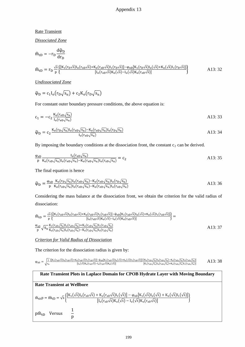
Appendix 13
Rate Transient
Dissociated Zone
m� tD = −rDdφ�DdrD
m� tD = rD√sp��K1�rD√s�Io�rsD√s�+Ko�rsD√s�I1�rD√s��−φsD�K1�rD√s�Io�√s�+Ko�√s�I1�rD√s��
�Io�rsD√s�Ko�√s�−Io�√s�Ko�rsD√s��� A13: 32
Undissociated Zone
φ�D = c1Io�rD�s𝑈𝑈� + c2Ko�rD�s𝑈𝑈�
For constant outer boundary pressure conditions, the above equation is:
c1 = −c2Ko�reD�s𝑢𝑢�Io�reD�s𝑢𝑢�
A13: 33
φ�D = c2Ko�rD�s𝑢𝑢�Io�reD�s𝑢𝑢�−Ko�reD�s𝑢𝑢�Io�rD�s𝑢𝑢�
Io�reD�s𝑢𝑢� A13: 34
By imposing the boundary conditions at the dissociation front, the constant c2 can be derived.
φsDp
Io�reD�s𝑢𝑢�Ko�rsD�s𝑢𝑢�Io�reD�s𝑢𝑢�−Ko�reD�s𝑢𝑢�Io�rsD�s𝑢𝑢�
= c2 A13: 35
The final equation is hence
φ�D = φsDp
Ko�rD�s𝑢𝑢�Io�reD�s𝑢𝑢�−Ko�reD�s𝑢𝑢�Io�rD�s𝑢𝑢�Ko�rsD�s𝑢𝑢�Io�reD�s𝑢𝑢�−Ko�reD�s𝑢𝑢�Io�rsD�s𝑢𝑢�
A13: 36
Considering the mass balance at the dissociation front, we obtain the criterion for the valid radius of
dissociation:
m� tD = √sp��K1�rsD√s�Io�rsD√s�+Ko�rsD√s�I1�rsD√s��−φ�sD�K1�rsD√s�Io�√s�+Ko�√s�I1�rsD√s��
�Io�rsD√s�Ko�√s�−Io�√s�Ko�rsD√s��� =
φsDp �s𝑉𝑉
K1�rsD�s𝑉𝑉�Io�reD�s𝑉𝑉�+Ko�reD�s𝑉𝑉�I1�rsD�s𝑉𝑉�Ko�rsD�s𝑉𝑉�Io�reD�s𝑉𝑉�−Ko�reD�s𝑉𝑉�Io�rsD�s𝑉𝑉�
A13: 37
Criterion for Valid Radius of Dissociation
The criterion for the dissociation radius is given by:
φsD = �ss𝑢𝑢
��K1�rsD√s�Io�rsD√s�+Ko�rsD√s�I1�rsD√s��−φ�sD�K1�rsD√s�Io�√s�+Ko�√s�I1�rsD√s����Io�√s�Ko�rsD√s�−Io�rsD√s�Ko�√s��
�Ko�rsD�s𝑢𝑢�Io�reD�s𝑢𝑢�−Ko�reD�s𝑢𝑢�Io�rsD�s𝑢𝑢���K1�rsD�s𝑢𝑢�Io�reD�s𝑢𝑢�+Ko�reD�s𝑢𝑢�I1�rsD�s𝑢𝑢��
A13: 38
Rate Transient Plots in Laplace Domain for CPOB Hydrate Layer with Moving Boundary
Rate Transient at Wellbore
m�tDp = mtD = √s ��K1�√s�Io�rsD√s� + Ko�rsD√s�I1�√s�� − φsD�K1�√s�Io�√s� + Ko�√s�I1�√s��
�Io�rsD√s�Ko�√s� − Io�√s�Ko�rsD√s���
pm� tD Versus 1p
199
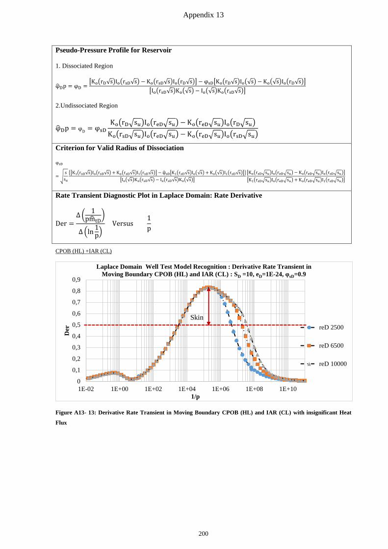
Appendix 13
Pseudo-Pressure Profile for Reservoir
1. Dissociated Region
φ�Dp = φD =�Ko�rD√s�Io�rsD√s� − Ko�rsD√s�Io�rD√s�� − φsD�Ko�rD√s�Io�√s� − Ko�√s�Io�rD√s��
�Io�rsD√s�Ko�√s� − Io�√s�Ko�rsD√s��
2.Undissociated Region
φ�Dp = φD = φsDKo�rD�s𝑈𝑈�Io�reD�s𝑈𝑈� − Ko�reD�s𝑈𝑈�Io�rD�s𝑈𝑈�
Ko�rsD�s𝑈𝑈�Io�reD�s𝑈𝑈� − Ko�reD�s𝑈𝑈�Io�rsD�s𝑈𝑈�
Criterion for Valid Radius of Dissociation
φsD
= �s
s𝑈𝑈��K1�rsD√s�Io�rsD√s� + Ko�rsD√s�I1�rsD√s�� − φ�sD�K1�rsD√s�Io�√s� + Ko�√s�I1�rsD√s���
�Io�√s�Ko�rsD√s� − Io�rsD√s�Ko�√s���Ko�rsD�s𝑈𝑈�Io�reD�s𝑈𝑈� − Ko�reD�s𝑈𝑈�Io�rsD�s𝑈𝑈���K1�rsD�s𝑈𝑈�Io�reD�s𝑈𝑈� + Ko�reD�s𝑈𝑈�I1�rsD�s𝑈𝑈��
Rate Transient Diagnostic Plot in Laplace Domain: Rate Derivative
Der =∆ � 1
pm� tD�
∆ �ln 1p�
Versus 1p
CPOB (HL) +IAR (CL)
Figure A13- 13: Derivative Rate Transient in Moving Boundary CPOB (HL) and IAR (CL) with insignificant Heat
Flux
0
0,1
0,2
0,3
0,4
0,5
0,6
0,7
0,8
0,9
1E-02 1E+00 1E+02 1E+04 1E+06 1E+08 1E+10
Der
1/p
Laplace Domain Well Test Model Recognition : Derivative Rate Transient in Moving Boundary CPOB (HL) and IAR (CL) : SD =10, eD=1E-24, φsD=0.9
reD 2500
reD 6500
reD 10000
Skin
200
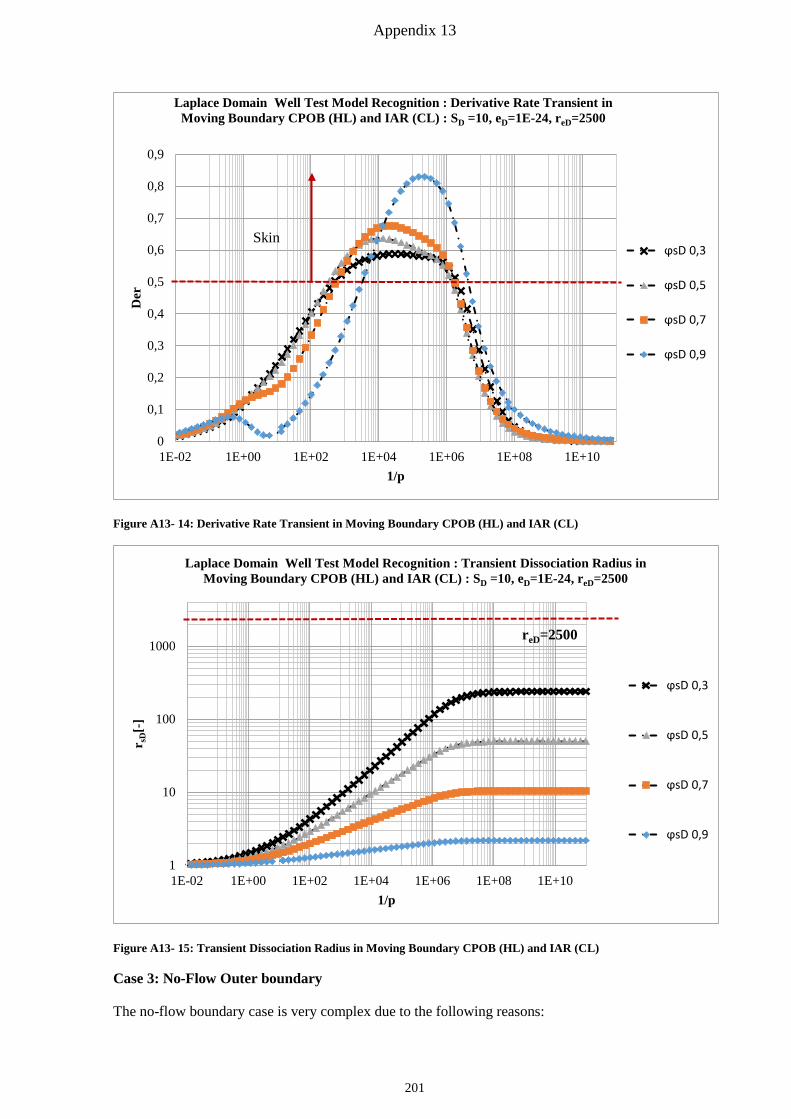
Appendix 13
Figure A13- 14: Derivative Rate Transient in Moving Boundary CPOB (HL) and IAR (CL)
Figure A13- 15: Transient Dissociation Radius in Moving Boundary CPOB (HL) and IAR (CL)
Case 3: No-Flow Outer boundary
The no-flow boundary case is very complex due to the following reasons:
0
0,1
0,2
0,3
0,4
0,5
0,6
0,7
0,8
0,9
1E-02 1E+00 1E+02 1E+04 1E+06 1E+08 1E+10
Der
1/p
Laplace Domain Well Test Model Recognition : Derivative Rate Transient in Moving Boundary CPOB (HL) and IAR (CL) : SD =10, eD=1E-24, reD=2500
ϕsD 0,3
ϕsD 0,5
ϕsD 0,7
ϕsD 0,9
Skin
1
10
100
1000
1E-02 1E+00 1E+02 1E+04 1E+06 1E+08 1E+10
r sD[-
]
1/p
Laplace Domain Well Test Model Recognition : Transient Dissociation Radius in Moving Boundary CPOB (HL) and IAR (CL) : SD =10, eD=1E-24, reD=2500
ϕsD 0,3
ϕsD 0,5
ϕsD 0,7
ϕsD 0,9
reD=2500
201
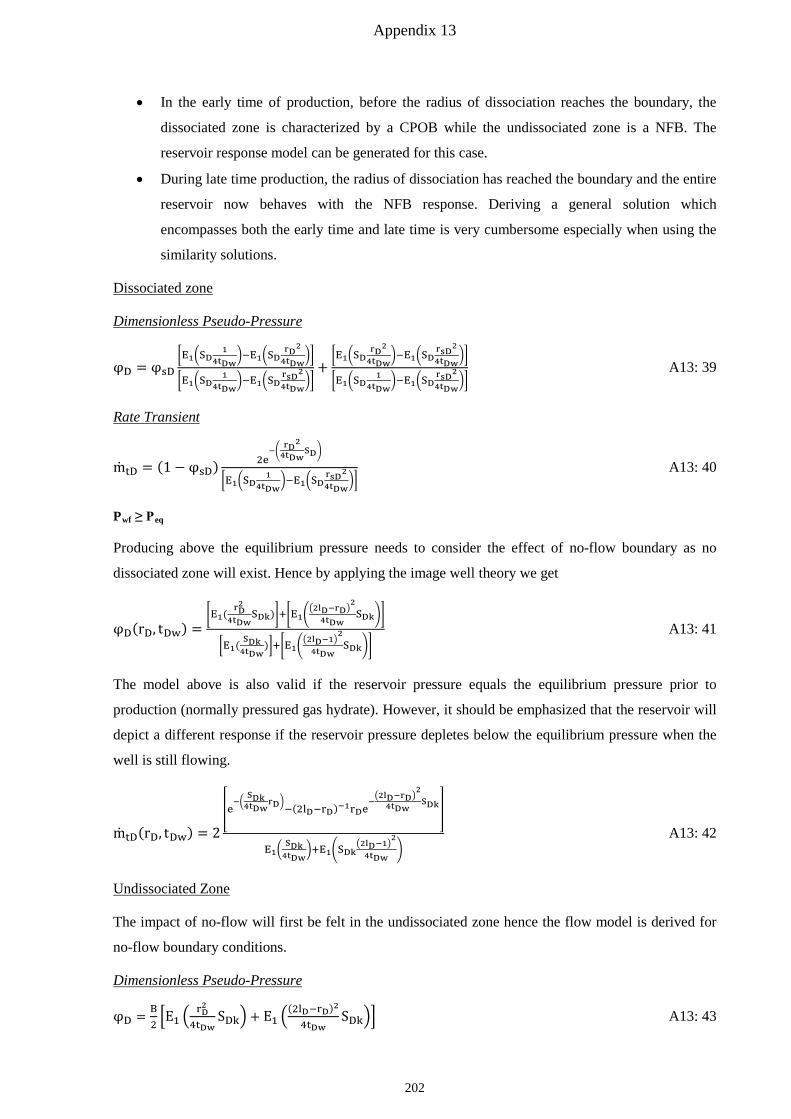
Appendix 13
• In the early time of production, before the radius of dissociation reaches the boundary, the
dissociated zone is characterized by a CPOB while the undissociated zone is a NFB. The
reservoir response model can be generated for this case.
• During late time production, the radius of dissociation has reached the boundary and the entire
reservoir now behaves with the NFB response. Deriving a general solution which
encompasses both the early time and late time is very cumbersome especially when using the
similarity solutions.
Dissociated zone
Dimensionless Pseudo-Pressure
φD = φsD�E1�SD
14tDw
�−E1�SDrD2
4tDw��
�E1�SD1
4tDw�−E1�SD
rsD2
4tDw��
+�E1�SD
rD2
4tDw�−E1�SD
rsD2
4tDw��
�E1�SD1
4tDw�−E1�SD
rsD2
4tDw��
A13: 39
Rate Transient
mtD = (1 − φsD) 2e−�
rD24tDw
SD�
�E1�SD1
4tDw�−E1�SD
rsD2
4tDw��
A13: 40
Pwf ≥ Peq
Producing above the equilibrium pressure needs to consider the effect of no-flow boundary as no
dissociated zone will exist. Hence by applying the image well theory we get
φD(rD, tDw) =�E1(
rD2
4tDwSDk)�+�E1�
�2lD−rD�2
4tDwSDk��
�E1( SDk4tDw
)�+�E1��2lD−1�
2
4tDwSDk��
A13: 41
The model above is also valid if the reservoir pressure equals the equilibrium pressure prior to
production (normally pressured gas hydrate). However, it should be emphasized that the reservoir will
depict a different response if the reservoir pressure depletes below the equilibrium pressure when the
well is still flowing.
mtD(rD, tDw) = 2
�e−�
SDk4tDw
rD�−(2lD−rD)−1rDe−�2lD−rD�
2
4tDwSDk�
E1�SDk4tDw
�+E1�SDk�2lD−1�
2
4tDw�
A13: 42
Undissociated Zone
The impact of no-flow will first be felt in the undissociated zone hence the flow model is derived for
no-flow boundary conditions.
Dimensionless Pseudo-Pressure
φD = B2�E1 �
rD2
4tDwSDk� + E1 �
(2lD−rD)2
4tDwSDk�� A13: 43
202
Appendix 13
The equation for the dimensionless pseudo-pressure in the un-dissociated zone is given thus:
φD = φsD�E1�
rD2
4tDwSDk�+E1�
�2lD−rD�2
4tDwSDk��
�E1�SDk𝑟𝑟sD
2
4tDw�+E1�SDk
�2lD−rsD�2
4tDw��
A13: 44
mtD = 2φsD
�e−�
SDk4tDw
rD2 �−(2lD−rD)−1rDe
−�2lD−rD�
2
4tDwSDk�
�E1�SDk𝑟𝑟sD
2
4tDw�+E1�SDk
�2lD−rsD�2
4tDw��
A13: 45
Using equating the mass rates at the crossover point the validity criterion for the radius of dissociation
is derived
Criterion for Valid Radius of Dissociation
For the dimensionless pseudo-pressures at the cross over point to be the same, the following condition
must be valid:
mtD = 2φsD
�e−�
SDk4tDw
𝑟𝑟sD2 �
−(2lD−𝐶𝐶sD)−1rsDe−�2lD−rsD�
2
4tDwSDk�
�E1�SDk𝑟𝑟sD2
4tDw�+E1�SDk
�2lD−rsD�2
4tDw��
= �1−φsD�2e
−�rsD
24tDw
SD�
�E1�SDk𝑟𝑟sD2
4tDw�+E1�SDk
�2lD−rsD�2
4tDw��
A13: 46
When the reservoir is fully dissociated and now acts similar to a normally pressured gas hydrate
reservoir, i.e. the reservoir pressure has depleted below the equilibrium pressure, the dimensionless
equilibrium pressure at the front is no longer constant but a function of time. By equating the
dimensionless pseudo-pressure solution for the normally pressured NFB and over-pressured NFB
reservoir, we get the following correction for the response:
φsD =2�E1�SD
lD2
4tDw��
�E1�SD1
4tDw�+E1�SD
�2lD−1�2
4tDw��
A13: 47
Solutions with Laplace Transformation (Solutions in Laplace Domain)
φ�D = c1Io�rD√s� + c2Ko�rD√s�
Dissociated Zone
The solutions given in Cases 1 and 2 earlier are also valid here for the dissociated zone.
Dimensionless Pseudo-Pressure
φ�D = �Ko�rD√s�Io�rsD√s�−Ko�rsD√s�Io�rD√s��−φsD�Ko�rD√s�Io�√s�−Ko�√s�Io�rD√s��p�Io�rsD√s�Ko�√s�−Io�√s�Ko�rsD√s��
A13: 48
Rate Transient
m� tD = rD√sp��K1�rD√s�Io�rsD√s�+Ko�rsD√s�I1�rD√s��−φsD�K1�rD√s�Io�√s�+Ko�√s�I1�rD√s��
�Io�rsD√s�Ko�√s�−Io�√s�Ko�rsD√s��� A13: 49
203
Appendix 13
Undissociated Zone
φ�D = c1Io�rD�su� + c2Ko�rD�su�
Dimensionless Pseudo-Pressure
The general equation takes the form
φ�D = c1�K1�reD�su�Io�rD�su�+I1�reD�su�Ko�rD�su��
K1�reD�su� A13: 50
φsDK1�reD�su�
𝑝𝑝�K1�reD�su�Io�rsD�su�+ I1�reD�su�Ko�rsD�su��= c1
φ�D = φsD�K1�reD�su�Io�rD�su� + I1�reD�su�Ko�rD�su���K1�reD�su�Io�rsD�su� + I1�reD�su�Ko�rsD�su��
The constant c1 is hence derived using the inner boundary condition at the dissociation front
m� tD = −rDdφ�DdrD
= c1rD�su�I1�reD�su�K1�rD�su�−K1�reD�su�I1�rD�su��
K1�reD�su� A13: 51
Dissociation front condition
m� tD = rD√sp��K1�rsD√s�Io�rsD√s� + Ko�rsD√s�I1�rsD√s�� − φsD�K1�rsD√s�Io�√s� + Ko�√s�I1�rsD√s��
�Io�rsD√s�Ko�√s� − Io�√s�Ko�rsD√s���
m� tD = √sp��K1�rsD√s�Io�rsD√s�+Ko�rsD√s�I1�rsD√s��−φsD�K1�rsD√s�Io�√s�+Ko�√s�I1�rsD√s��
�Io�rsD√s�Ko�√s�−Io�√s�Ko�rsD√s��� =
φsD�su𝐶𝐶
�I1�reD�su�K1�rsD�su�−K1�reD�su�I1�rsD�su���K1�reD�su�Io�rsD�su�+I1�reD�su�Ko�rsD�su��
A13: 52
Criterion for Valid Radius of Dissociation
φsD = �ssu𝐴𝐴 �K1�reD�su�Io�rsD�su�+I1�reD�su�Ko�rsD�su���I1�reD�su�K1�rsD�su�−K1�reD�su�I1�rsD�su��
A13: 53
Where,
𝐴𝐴 = ��K1�rsD√s�Io�rsD√s�+Ko�rsD√s�I1�rsD√s��−φsD�K1�rsD√s�Io�√s�+Ko�√s�I1�rsD√s���Io�rsD√s�Ko�√s�−Io�√s�Ko�rsD√s��
� A13: 54
When rsD=reD, the mass balance at the dissociation front reduces to
��K1�reD√s�Io�reD√s� + Ko�reD√s�I1�reD√s��
�K1�reD√s�Io�√s� + Ko�√s�I1�reD√s��� = φsD
By inserting the function for the pseudo-pressure at the boundary, the rate transient equation takes the
following form at the wellbore and boundary:
m� tD(rD = 1, p) =√sp��I1�reD√s�K1�√s�−K1�reD√s�I1�√s��Ko�√s�I1�reD√s�+ K1�reD√s�Io�√s�
�
204
Appendix 13
m� tD(reD = 1, p) = 0
This further validates the model
Rate Transient Plots in Laplace Domain for NFB Hydrate Layer with Moving Boundary
Rate Transient at Wellbore
m� tD =√sp��K1�√s�Io�rsD√s� + Ko�rsD√s�I1�√s�� − φsD�K1�√s�Io�√s� + Ko�√s�I1�√s��
�Io�rsD√s�Ko�√s� − Io�√s�Ko�rsD√s���
Plot
pm� tD Versus 1p
Pseudo-Pressure Profile for Reservoir (Pwf<Peq)
1. Dissociated Region
φ�D =1p�Ko�rD√s�Io�rsD√s� − Ko�rsD√s�Io�rD√s�� − φsD�Ko�rD√s�Io�√s� − Ko�√s�Io�rD√s��
�Io�rsD√s�Ko�√s� − Io�√s�Ko�rsD√s��
2.Undissociated Region
φ�D =φsD
p�K1�reD�su�Io�rD�su� + I1�reD�su�Ko�rD�su���K1�reD�su�Io�rsD�su� + I1�reD�su�Ko�rsD�su��
For: rsD<reD
φsD = constant
For: rsD=reD
φ�Dp = φsD =�K1�reD√𝑉𝑉�Io�rD√s� + I1�reD√s�Ko�rD√s���K1�reD√s�Io�√s� + I1�reD√s�Ko�√𝑉𝑉��
Plot
𝑝𝑝φ�D Versus rD
Pseudo-Pressure Profile for Reservoir (Pwf ≥ Peq during Production)
1. Un-dissociated Region (Reservoir depicts a conventional reservoir)
φ�D =�K1�reD�su�Io�rD�su� + I1�reD�su�Ko�rD�su��
𝑝𝑝�K1�reD�su�Io�rsD�su� + I1�reD�su�Ko�rsD�su��
Plot
𝑝𝑝φ�D Versus rD
205
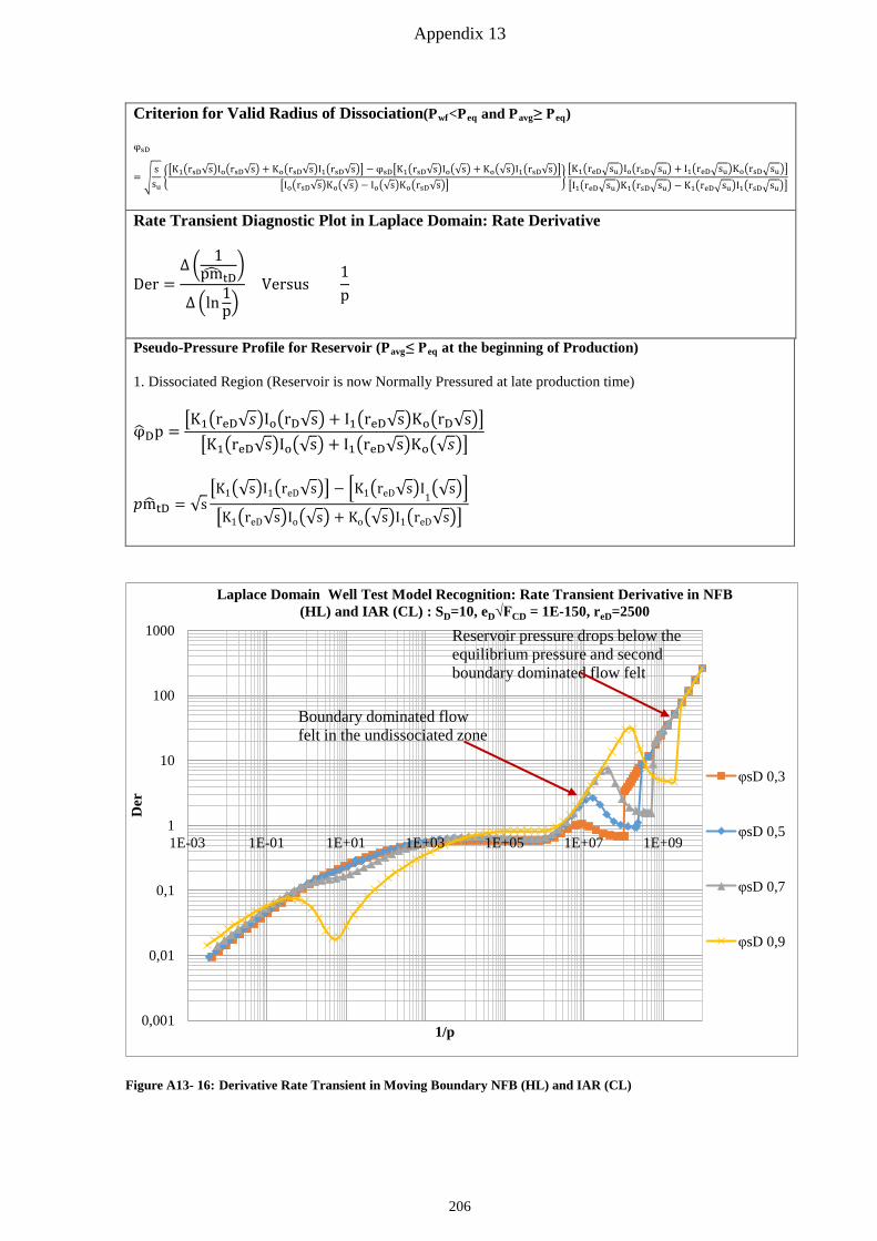
Appendix 13
Criterion for Valid Radius of Dissociation(Pwf<Peq and Pavg≥ Peq)
φsD
= �s
su��K1�rsD√s�Io�rsD√s� + Ko�rsD√s�I1�rsD√s�� − φsD�K1�rsD√s�Io�√s� + Ko�√s�I1�rsD√s��
�Io�rsD√s�Ko�√s� − Io�√s�Ko�rsD√s����K1�reD�su�Io�rsD�su� + I1�reD�su�Ko�rsD�su���I1�reD�su�K1�rsD�su� − K1�reD�su�I1�rsD�su��
Rate Transient Diagnostic Plot in Laplace Domain: Rate Derivative
Der =∆ � 1
pm� tD�
∆ �ln 1p�
Versus 1p
Pseudo-Pressure Profile for Reservoir (Pavg≤ Peq at the beginning of Production)
1. Dissociated Region (Reservoir is now Normally Pressured at late production time)
φ�Dp =�K1�reD√𝑉𝑉�Io�rD√s�+ I1�reD√s�Ko�rD√s���K1�reD√s�Io�√s� + I1�reD√s�Ko�√𝑉𝑉��
𝑝𝑝m� tD = √s�K1�√s�I1�reD√s�� − �K1�reD√s�I
1�√s��
�K1�reD√s�Io�√s� + Ko�√s�I1�reD√s��
Figure A13- 16: Derivative Rate Transient in Moving Boundary NFB (HL) and IAR (CL)
0,001
0,01
0,1
1
10
100
1000
1E-03 1E-01 1E+01 1E+03 1E+05 1E+07 1E+09
Der
1/p
Laplace Domain Well Test Model Recognition: Rate Transient Derivative in NFB (HL) and IAR (CL) : SD=10, eD√FCD = 1E-150, reD=2500
φsD 0,3
φsD 0,5
φsD 0,7
φsD 0,9
Boundary dominated flow felt in the undissociated zone
Reservoir pressure drops below the equilibrium pressure and second boundary dominated flow felt
206

Appendix 13
Figure A13- 17: Transient Dissociation Radius in Moving Boundary NFB (HL) and IAR (CL)
1
10
100
1000
10000
1E-02 1E+00 1E+02 1E+04 1E+06 1E+08 1E+10
r sD [-
]
1/p
Laplace Domain Well Test Model Recognition : Transient Dissociation Radius in Moving Boundary CPOB (HL) and IAR (CL) : SD =10, eD=1E-24, reD=2500
φsD 0,3
φsD 0,5
φsD 0,7
φsD 0,9
207
Appendix 14
Appendix 14: Solutions to the Diffusivity Equation in Crossflow layer
Crossflow problems will be expected in Class 1 and 2 gas hydrate reservoirs if the boundary between
the free fluid layer and the hydrate layer is permeable. Depending on the layer chosen for production,
different crossflow regimes could be analyzed. Moreover, boundary conditions imposed on outer
boundaries of the crossflow layer is very dependent on the layer of production.
Conventionally, for the hydrate reservoir to be considered for production, the layer above the hydrate
layer should be impermeable (cap rock). For this reason, we consider no-flow at the outer boundary of
the hydrate layer and just heat influx due to heat conduction from the cap rock is considered for the
hydrate dissociation process. However, the effects of hydrate dissociation at the outer boundary of the
hydrate layer could have significant influence of the reservoir response.
For cases where the production takes place in the free fluid layer, at the time pressure depression
reaches the upper boundary of the hydrate layer, temperature depressions are also experienced due to
the endothermic nature of hydrate dissociation. For this reason, dissociation as a result of heat flux
from conduction will occur basically at the boundary and is controlled by the temperature depression
at the boundary. When the hydrates dissociate at the boundary, the pressure at the dissociation front
increases which implies, depending on the rate of hydrate dissociation, the pressure depression at the
reservoir boundary could be supported by hydrate dissociation due to heat influx. The effect of
pressure support at the boundary is a known phenomenon is usually described as the constant pressure
outer boundary condition where pressure depression at the boundary is zero due to fluid influx. With a
proper definition of the boundary conditions, this effect can be characterized with a rigorous model.
However, other simplifications of the model can be made from the following assumptions:
• Constant Pressure Outer Boundary in Hydrate Layer: High hydrate dissociation at the outer
boundary due to heat influx is very significant and contributes to pressure maintenance.
• No-flow Outer Boundary in Hydrate Layer: Insignificant hydrate dissociation at the outer
boundary due to heat influx.
With these models, we can address the diffusivity equations for the crossflow layers. In the late phase
of production, the effects of heat conduction could have become noticeable and hence an accelerated
hydrate dissociation which also caused an increase in gas production.
Solution to the Diffusivity Equation in Crossflow Layer
Crossflow Layer is Hydrate Layer
∆x ∗ ∆y ∗ ∆(ρg ∗ wg,T) + ∆x ∗ ∆y ∗ ∆(ρw ∗ ww,T) = ∆x ∗ ∆y ∗ ∆z ∆�Sg∅ρg�
∆t+ ∆x ∗ ∆y ∗ ∆z ∆(Sw∅ρw)
∆t+ ∆x ∗ ∆y ∗ ∆z ∆(Sh∅ρh)
∆t A14: 1
Crossflow Layer is Free Fluid Layer
∆x ∗ ∆y ∗ ∆(ρg ∗ wg,T) + ∆x ∗ ∆y ∗ ∆(ρw ∗ww,T) = ∆x ∗ ∆y ∗ ∆z ∆�Sg∅ρg�∆t
+ ∆x ∗ ∆y ∗ ∆z ∆(Sw∅ρw)∆t
A14: 2
208
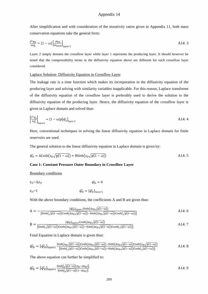
Appendix 14
After simplification and with consideration of the storativity ratios given in Appendix 11, both mass
conservation equations take the general form:
∂2φD∂zD
2 = [1 − ω] � ∂φD∂tDwD
�layer 2
A14: 3
Layer 2 simply denotes the crossflow layer while layer 1 represents the producing layer. It should however be
noted that the compressibility terms in the diffusivity equation above are different for each crossflow layer
considered.
Laplace Solution- Diffusivity Equation in Crossflow Layer
The leakage rate is a time function which makes its incorporation in the diffusivity equation of the
producing layer and solving with similarity variables inapplicable. For this reason, Laplace transforms
of the diffusivity equation of the crossflow layer is preferably used to derive the solution to the
diffusivity equation of the producing layer. Hence, the diffusivity equation of the crossflow layer is
given in Laplace domain and solved thus:
�∂2φD�
∂zD2 �
layer2= [1−ω]p�φD� �
layer 2 A14: 4
Here, conventional techniques in solving the linear diffusivity equation in Laplace domain for finite
reservoirs are used.
The general solution to the linear diffusivity equation in Laplace domain is given by:
φD� = ACosh�zD�p[1 − ω]� + BSinh�zD�p[1 − ω]� A14: 5
Case 1: Constant Pressure Outer Boundary in Crossflow Layer
Boundary conditions
zD=ΔzD φD� = 0
zD=1 φD� = [𝜑𝜑𝐷𝐷� ]𝑙𝑙𝐶𝐶𝑙𝑙𝑈𝑈𝐶𝐶1
With the above boundary conditions, the coefficients A and B are given thus:
A = −[φD� ]layer1Sinh�∆zD�p[1−ω]�
�Sinh��p[1−ω]�Cosh�∆zD�p[1−ω]�−Sinh�∆zD�p[1−ω]�Cosh��p[1−ω]�� A14: 6
B =[φD� ]layer1Cosh�∆zD�p[1−ω]�
�Sinh��p[1−ω]�Cosh�∆zD�p[1−ω]�−Sinh�∆zD�p[1−ω]�Cosh��p[1−ω]�� A14: 7
Final Equation in Laplace domain is given thus:
φD� = [φD� ]layer1Sinh�zD�p[1−ω]�Cosh�∆zD�p[1−ω]�−Sinh�∆zD�p[1−ω]�Cosh�zD�p[1−ω]��Sinh��p[1−ω]�Cosh�∆zD�p[1−ω]�−Sinh�∆zD�p[1−ω]�Cosh��p[1−ω]��
A14: 8
The above equation can further be simplified to:
φD� = [φD� ]layer1Sinh��p[1−ω](zD−∆zD)�Sinh��p[1−ω](1−∆zD)�
A14: 9
209
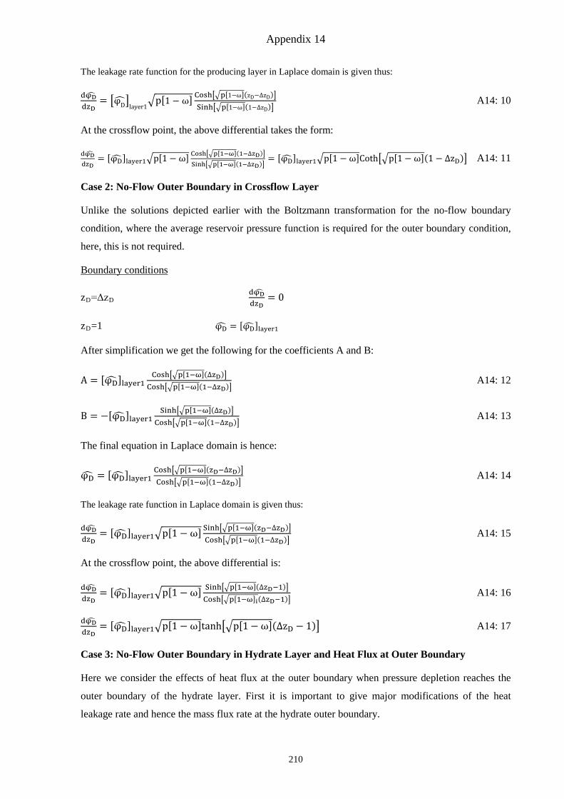
Appendix 14
The leakage rate function for the producing layer in Laplace domain is given thus:
dφD�dzD
= �φD��layer1
�p[1 − ω] Cosh��p[1−ω](zD−∆zD)�Sinh��p[1−ω](1−∆zD)�
A14: 10
At the crossflow point, the above differential takes the form:
dφD�dzD
= [φD� ]layer1�p[1 − ω] Cosh��p[1−ω](1−∆zD)�Sinh��p[1−ω](1−∆zD)�
= [φD� ]layer1�p[1 − ω]Coth��p[1 − ω](1 − ∆zD)� A14: 11
Case 2: No-Flow Outer Boundary in Crossflow Layer
Unlike the solutions depicted earlier with the Boltzmann transformation for the no-flow boundary
condition, where the average reservoir pressure function is required for the outer boundary condition,
here, this is not required.
Boundary conditions
zD=ΔzD dφD�dzD
= 0
zD=1 φD� = [φD� ]layer1
After simplification we get the following for the coefficients A and B:
A = [φD� ]layer1Cosh��p[1−ω](∆zD)�
Cosh��p[1−ω](1−∆zD)� A14: 12
B = −[φD� ]layer1Sinh��p[1−ω](∆zD)�
Cosh��p[1−ω](1−∆zD)� A14: 13
The final equation in Laplace domain is hence:
φD� = [φD� ]layer1Cosh��p[1−ω](zD−∆zD)�Cosh��p[1−ω](1−∆zD)�
A14: 14
The leakage rate function in Laplace domain is given thus:
dφD�dzD
= [φD� ]layer1�p[1 −ω] Sinh��p[1−ω](zD−∆zD)�Cosh��p[1−ω](1−∆zD)�
A14: 15
At the crossflow point, the above differential is:
dφD�dzD
= [φD� ]layer1�p[1 −ω] Sinh��p[1−ω](∆zD−1)�Cosh��p[1−ω]i(∆zD−1)�
A14: 16
dφD�dzD
= [φD� ]layer1�p[1 −ω]tanh��p[1−ω](∆zD − 1)� A14: 17
Case 3: No-Flow Outer Boundary in Hydrate Layer and Heat Flux at Outer Boundary
Here we consider the effects of heat flux at the outer boundary when pressure depletion reaches the
outer boundary of the hydrate layer. First it is important to give major modifications of the heat
leakage rate and hence the mass flux rate at the hydrate outer boundary.
210
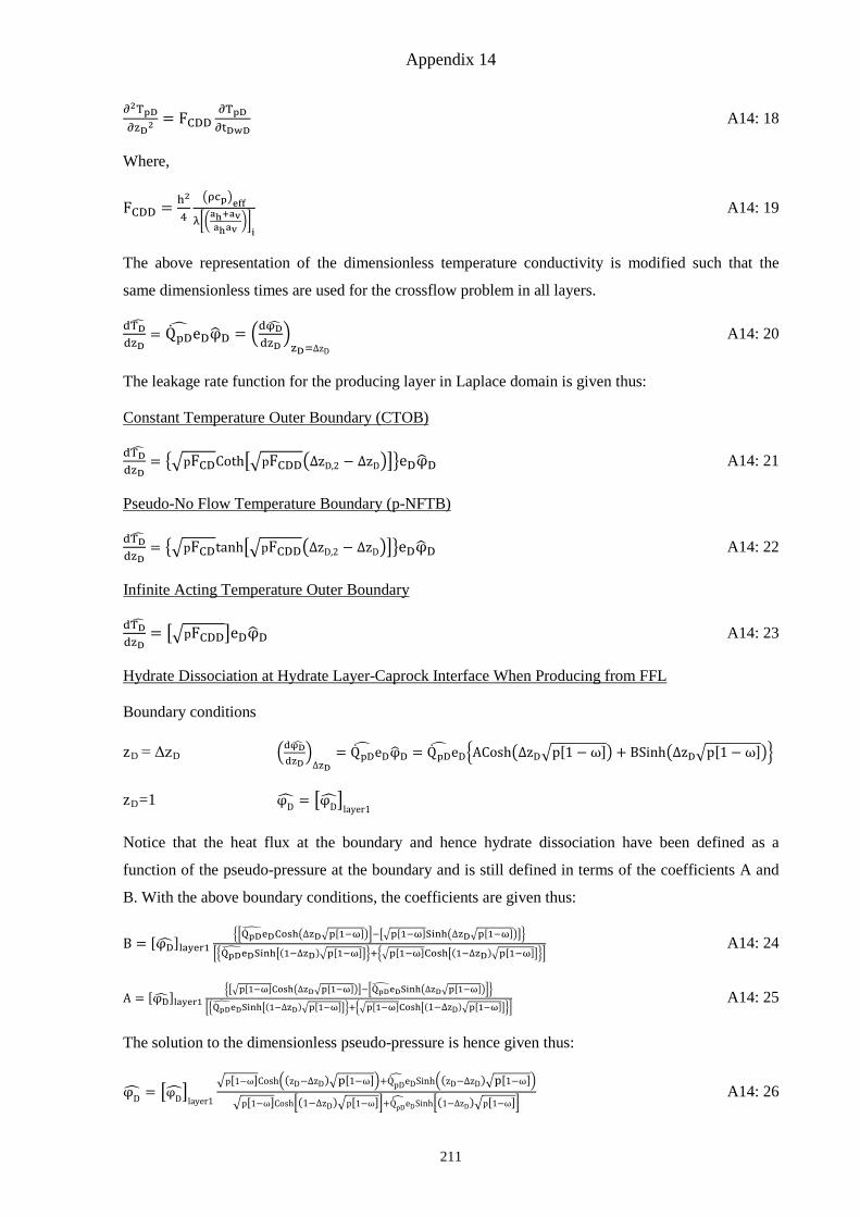
Appendix 14
∂2TpD∂zD2
= FCDD∂TpD∂tDwD
A14: 18
Where,
FCDD = h2
4
�ρcp�effλ��ah+avahav
��i
A14: 19
The above representation of the dimensionless temperature conductivity is modified such that the
same dimensionless times are used for the crossflow problem in all layers.
dTD�
dzD= QpD
� eDφ�D = �dφD�dzD
�zD=∆zD
A14: 20
The leakage rate function for the producing layer in Laplace domain is given thus:
Constant Temperature Outer Boundary (CTOB)
dTD�
dzD= ��pFCDCoth��pFCDD�∆zD,2 − ∆zD���eDφ�D A14: 21
Pseudo-No Flow Temperature Boundary (p-NFTB)
dTD�
dzD= ��pFCDtanh��pFCDD�∆zD,2 − ∆zD���eDφ�D A14: 22
Infinite Acting Temperature Outer Boundary
dTD�
dzD= ��pFCDD�eDφ�D A14: 23
Hydrate Dissociation at Hydrate Layer-Caprock Interface When Producing from FFL
Boundary conditions
zD = ΔzD �dφD�dzD
�∆zD
= QpD� eDφ�D = QpD
� eD�ACosh�∆zD�p[1 − ω]� + BSinh�∆zD�p[1 − ω]��
zD=1 φD� = �φD��layer1
Notice that the heat flux at the boundary and hence hydrate dissociation have been defined as a
function of the pseudo-pressure at the boundary and is still defined in terms of the coefficients A and
B. With the above boundary conditions, the coefficients are given thus:
B = [φD� ]layer1��QpD�eDCosh�∆zD�p[1−ω]��−��p[1−ω]Sinh�∆zD�p[1−ω]���
��QpD�eDSinh�(1−∆zD)�p[1−ω]��+��p[1−ω]Cosh�(1−∆zD)�p[1−ω]��� A14: 24
A = [φD� ]layer1���p[1−ω]Cosh�∆zD�p[1−ω]��−�QpD�eDSinh�∆zD�p[1−ω]���
��QpD�eDSinh�(1−∆zD)�p[1−ω]��+��p[1−ω]Cosh�(1−∆zD)�p[1−ω]��� A14: 25
The solution to the dimensionless pseudo-pressure is hence given thus:
φD� = �φD��layer1
�p[1−ω]Cosh�(zD−∆zD)�p[1−ω]�+QpD� eDSinh�(zD−∆zD)�p[1−ω]�
�p[1−ω]Cosh�(1−∆zD)�p[1−ω]�+QpD� eDSinh�(1−∆zD)�p[1−ω]�
A14: 26
211
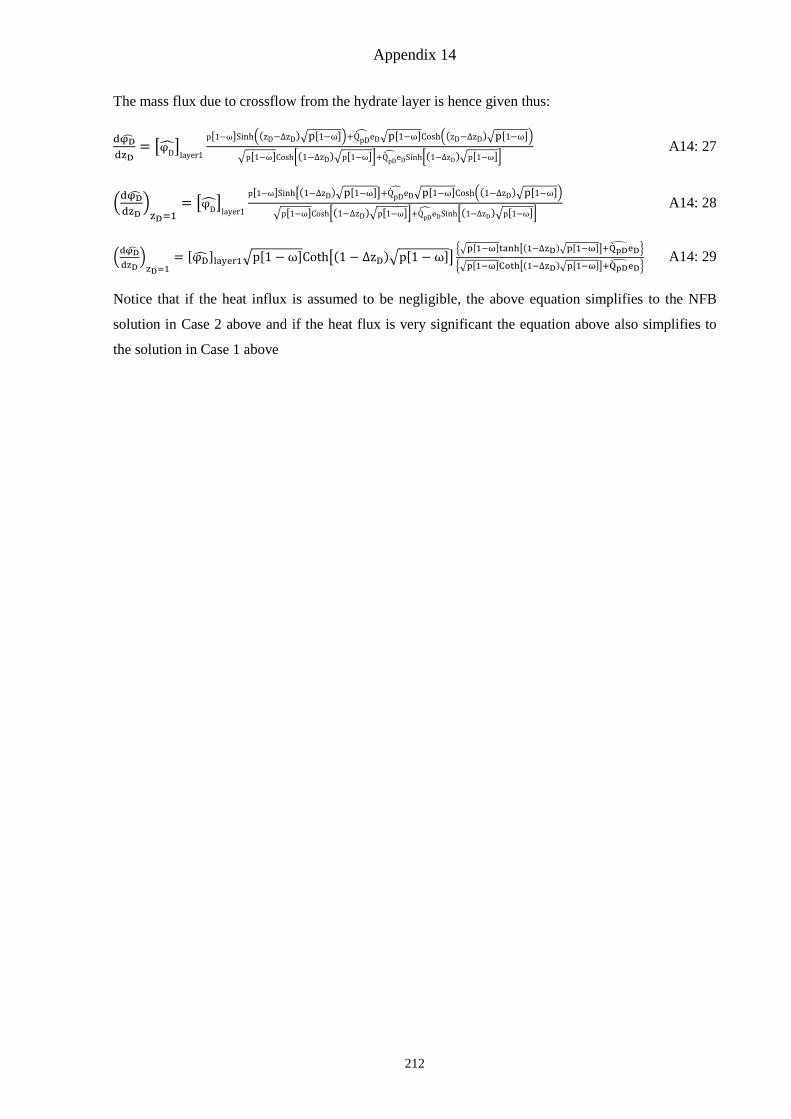
Appendix 14
The mass flux due to crossflow from the hydrate layer is hence given thus:
dφD�dzD
= �φD��layer1
p[1−ω]Sinh�(zD−∆zD)�p[1−ω]�+QpD� eD�p[1−ω]Cosh�(zD−∆zD)�p[1−ω]�
�p[1−ω]Cosh�(1−∆zD)�p[1−ω]�+QpD� eDSinh�(1−∆zD)�p[1−ω]�
A14: 27
�dφD�dzD
�zD=1
= �φD��layer1
p[1−ω]Sinh�(1−∆zD)�p[1−ω]�+QpD� eD�p[1−ω]Cosh�(1−∆zD)�p[1−ω]�
�p[1−ω]Cosh�(1−∆zD)�p[1−ω]�+QpD� eDSinh�(1−∆zD)�p[1−ω]�
A14: 28
�dφD�dzD
�zD=1
= [φD� ]layer1�p[1 −ω]Coth�(1 − ∆zD)�p[1 −ω]���p[1−ω]tanh�(1−∆zD)�p[1−ω]�+QpD�eD�
��p[1−ω]Coth�(1−∆zD)�p[1−ω]�+QpD�eD� A14: 29
Notice that if the heat influx is assumed to be negligible, the above equation simplifies to the NFB
solution in Case 2 above and if the heat flux is very significant the equation above also simplifies to
the solution in Case 1 above
212

Appendix 15
Appendix 15: Diffusivity Problems in Class 1 and 2 Gas Hydrate Reservoirs (Crossflow)
Analogue the diffusivity equation derived in Appendix 1 and Appendix 5 we also derive the
diffusivity equation for Classes 1 and 2 gas hydrate reservoirs.
Hydrate Layer is Producing Layer
Here, the mass influx from the free fluid layer and the hydrate mass dissociated from each heat source
component has to be considered.
∂2φ∂rD
2 + 1rD
∂ ∂rD
− λh2
QDrw2
hdk�ρt�krɳ �t
��dTeqdp
� (φi − φ) − �rw2
∆z2
kv2kh1
∂φ∂z�layer 2
− cp∆Thd
� rw2
∆z2
kv2kh1
∂φ∂z�layer 2
= �SDah,i� ∂φ∂t
A15: 1
∂2φ∂rD
2 + 1rD
∂φ ∂rD
− γD�φ𝑖𝑖 − φ� − � rw2
∆z2
kv2kh1
∂φ∂z�layer 2
− cp∆Thd
� rw2
∆z2
kv2kh1
∂φ∂z�layer 2
= � 1ah
∂φ∂t�PL
A15: 2
∂2φD∂rD
2 + 1rD
∂φD ∂rD
− γDφD −rw2
∆z2∆z1
kv2kh1
�∂φD∂zD
�layer 2
− cp∆Thd
� rw2
∆z2∆z1
kv2kh1
∂φD∂zD
�layer 2
= � 1ah
∂φD∂t�PL
A15: 3
∂2φD∂rD
2 + 1rD
∂φD ∂rD
− γDφD − δD �∂φD∂zD
�layer 2
− cp∆Thd
δD �∂φD∂zD
�layer 2
= ω� ∂φD∂tDwD
�layer 1
A15: 4
∂2φD∂rD
2 + 1rD
∂φD ∂rD
− γDφD − δD(1 + θD) �∂φD∂zD
�layer 2
= ω � ∂φD∂tDwD
�layer 1
A15: 5
Where,
δD = rw2
∆z2∆z1
kv2kh1
A15: 6
θD = cp∆Thd
A15: 7
tDwD = t
��ah+avahav
��i
A15: 8
1ah
= SDah,id
= (ρcT)eff,id�ρtk�
krɳ �t
�id
rw2 �(ρcT)eff
(ρcT)eff,id
�ρtk�krɳ �t
�id
�ρtk�krɳ �t
�+ c
hd(ρcT)eff,id
�ρtk�krɳ �t
�id
�ρtk�krɳ �t
�� A15: 9
(ρcT)eff = �ρgcT,g + ρwcT,w� A15: 10
cT,g = Sgcg + SgcF + SHcF �BgEg
�BgEg+BwEw�� A15: 11
cT,w = Swcw + SwcF + SHcF �EwBw
�BgEg+BwEw�� A15: 12
c = �cp,gSgρg �T�cg+cF�
�dTeqdp �
+ 1� + cp,wSwρw �T(cw+cF)
�dTeqdp �
+ 1� + cp,HSHρH �T(cF)
�dTeqdp �
+ 1� + cp,m(1−∅)∅
ρm + SHρHdhddTeq
� �dTeqdp
� A15: 13
γD > 0 and θD > 0
Note that if the kinetic model is used, the diffusivity equation simply takes the form:
213
Appendix 15
Kinetic Model
∂2φ∂rD
2 + 1rD
∂φ ∂rD
− γDk�φ𝑖𝑖 − φ� − � rw2
∆z2
kv2kh1
∂φ∂z�layer 2
= �SD𝑘𝑘
ah,i
∂φ∂t�PL
A15: 14
∂2φD∂rD
2 + 1rD
∂φD ∂rD
− γDkφD − δD �∂φD∂zD
�layer 2
= ω� ∂φD∂tDwD
�layer 1
A15: 15
Free Fluid Layer is Producing Layer
Here the mass leakage rate from the hydrate layer is quantified in one term as this is already reflected
in the diffusivity equation of the crossflow layer (hydrate layer) incorporated in the diffusivity
equation of the free fluid layer.
Hence:
∂2φ∂rD
2 + 1rD
∂ ∂rD
− � rw2
∆z2
kv2kh1
∂φ∂z�layer 2
= �𝑆𝑆𝐷𝐷𝐷𝐷ah,i� ∂φ∂t
A15: 16
∂2φD∂rD
2 + 1rD
∂φD ∂rD
− δD �∂φD∂zD
�layer 2
= ω� ∂φD∂tDwD
�layer 1
A15: 17
Where,
1ah
= SDkah,id
= (ρcT)eff,id�ρtk�
krɳ �t
�id
rw2 �(ρcT)eff
(ρcT)eff,id
�ρtk�krɳ �t
�id
�ρtk�krɳ �t
�� A15: 18
(ρcT)eff = ρgcT,g + ρwcT,w A15: 19
cT,g = Sgcg + SgcF A15: 20
cT,w = Swcw + SwcF A15: 21
δD = rw2
∆z2∆z1
kv2kh1
A15: 22
tDwD = t
��ah+avahav
��i
A15: 23
γD = 0 and θD = 0
214
Appendix 16
Appendix 16: Solutions to the Diffusivity Equation when producing from the Free Fluid
Layer
The diffusivity equation to the crossflow problem when producing from the free fluid layer is given
by:
∂2φD∂rD
2 + 1rD
∂φD ∂rD
− δD �∂[φD] layer2
∂zD�𝑧𝑧𝐷𝐷=1
= ω ∂φD∂tDwD
A16: 1
Using the Laplace transformation, the diffusivity equation above takes the form:
∂2φ�D∂rD2
+ 1rD
∂φ�D ∂rD
− δD �∂[φ�D] layer2
∂zD�𝑧𝑧𝐷𝐷=1
= ωpφ�D A16: 2
From the solutions of the crossflow layer given in Appendix 14, we introduce use the general form of
the solution for NFB with heat flux which has been shown to consider true NFB and CPOB all
depending on the rate of heat flux hence hydrate dissociation at the boundary.
Mass Influx from Hydrate Layer
�∂�φD� �layer2
∂zD�zD=1
= [φD� ]layer1�p[1 − ω]Coth�(1 − ∆zD)�p[1 − ω]���p[1−ω]tanh�(1−∆zD)�p[1−ω]�+QpD�eD�
��p[1−ω]Coth�(1−∆zD)�p[1−ω]�+QpD�eD�
The general form of the above equations can be written thus:
dφD�dzD
= [φD� ]layer1Mi A16: 3
Hence the diffusivity equation can be written thus:
∂2φ�D∂rD2
+ 1rD
∂φ�D ∂rD
− δDMiφD� = ωpφ�D A16: 4
∂2φ�D∂rD2
+ 1rD
∂φ�D ∂rD
− (δDMi + ωp)φ�D = 0 A16: 5
∂2φ�D∂rD2
+ 1rD
∂φ�D ∂rD
− λD2φ�D = 0 A16: 6
rD2∂2φ�D∂rD2
+ rD∂φ�D ∂rD
− rD2λD2φ�D = 0 A16: 7
As was done in Appendix 7, the above equation can be transformed into the modified Bessel equation
given in the form:
β2φ�D′′ + β2φ�D
′ − (β2 + 0)φ�D = 0 A16: 8
The solution to modified Bessel equation is given thus:
General Solution in Laplace Domain
φ�D = c1Io(rDλD) + c2Ko(rDλD) A16: 9
215

Appendix 16
Where,
λD = �(δDMi + ωp) A16: 10
φ�D′ = ∂φ�D
∂rD A16: 11
β = rDλD A16: 12
Case 1: Constant Terminal Pressure Solutions
Case 1a: Infinite Acting Reservoir
For the infinite acting system, the coefficient c1 equals zero and by using the inner boundary
condition, the solutions in Laplace domain are given thus:
Inner Boundary
c2 = 1pKo(λD) A16: 13
Dimensionless Pseudo-Pressure
φ�D = Ko(rDλD)pKo(λD) A16: 14
Dimensionless Flow rate
m� tD = −rDdφ�DdrD
= rDλDK1(rDλD)pKo(λD) A16: 15
Rate Transient Plot in Laplace Domain
pm� tD Versus 1p
φ�Dp Versus rD
Der =∆� 1
pm� tD�
∆�1p� Versus 1
p
Hydrate Layer Parameters
ω ΔzD δD
1,00E-05 10 0,0001
216
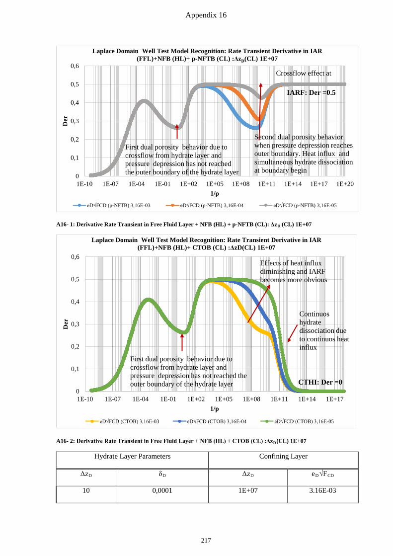
Appendix 16
A16- 1: Derivative Rate Transient in Free Fluid Layer + NFB (HL) + p-NFTB (CL): ΔzD (CL) 1E+07
A16- 2: Derivative Rate Transient in Free Fluid Layer + NFB (HL) + CTOB (CL) :ΔzD(CL) 1E+07
0
0,1
0,2
0,3
0,4
0,5
0,6
1E-10 1E-07 1E-04 1E-01 1E+02 1E+05 1E+08 1E+11 1E+14 1E+17 1E+20
Der
1/p
Laplace Domain Well Test Model Recognition: Rate Transient Derivative in IAR (FFL)+NFB (HL)+ p-NFTB (CL) :ΔzD(CL) 1E+07
eD√FCD (p-NFTB) 3,16E-03 eD√FCD (p-NFTB) 3,16E-04 eD√FCD (p-NFTB) 3,16E-05
First dual porosity behavior due to crossflow from hydrate layer and pressure depression has not reached the outer boundary of the hydrate layer
Second dual porosity behavior when pressure depression reaches outer boundary. Heat influx and simultaneous hydrate dissociation at boundary begin
IARF: Der =0.5
Crossflow effect at
0
0,1
0,2
0,3
0,4
0,5
0,6
1E-10 1E-07 1E-04 1E-01 1E+02 1E+05 1E+08 1E+11 1E+14 1E+17
Der
1/p
Laplace Domain Well Test Model Recognition: Rate Transient Derivative in IAR (FFL)+NFB (HL)+ CTOB (CL) :ΔzD(CL) 1E+07
eD√FCD (CTOB) 3,16E-03 eD√FCD (CTOB) 3,16E-04 eD√FCD (CTOB) 3,16E-05
CTHI: Der =0
Effects of heat influx diminishing and IARF becomes more obvious
First dual porosity behavior due to crossflow from hydrate layer and pressure depression has not reached the outer boundary of the hydrate layer
Continuos hydrate dissociation due to continuos heat influx
Hydrate Layer Parameters Confining Layer
ΔzD δD ΔzD eD√FCD
10 0,0001 1E+07 3.16E-03
217
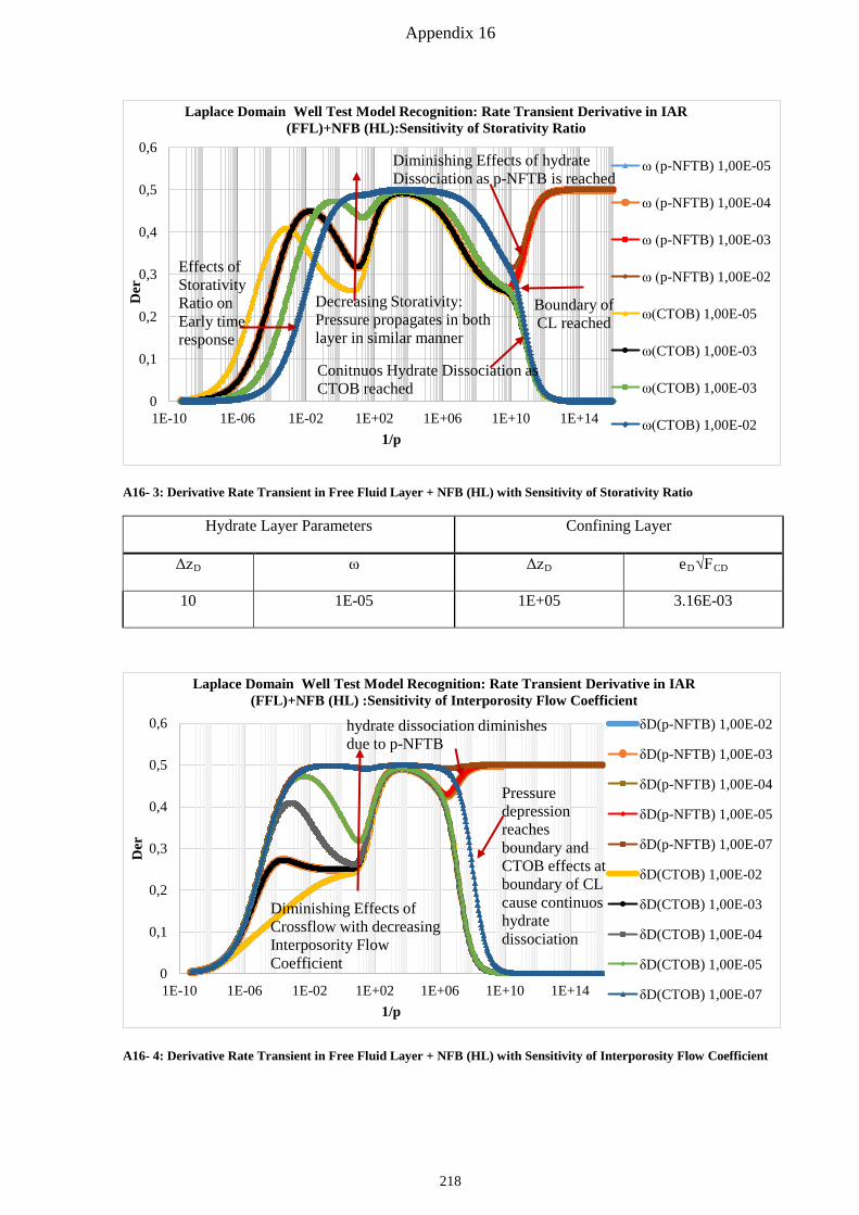
Appendix 16
A16- 3: Derivative Rate Transient in Free Fluid Layer + NFB (HL) with Sensitivity of Storativity Ratio
A16- 4: Derivative Rate Transient in Free Fluid Layer + NFB (HL) with Sensitivity of Interporosity Flow Coefficient
0
0,1
0,2
0,3
0,4
0,5
0,6
1E-10 1E-06 1E-02 1E+02 1E+06 1E+10 1E+14
Der
1/p
Laplace Domain Well Test Model Recognition: Rate Transient Derivative in IAR (FFL)+NFB (HL):Sensitivity of Storativity Ratio
ω (p-NFTB) 1,00E-05
ω (p-NFTB) 1,00E-04
ω (p-NFTB) 1,00E-03
ω (p-NFTB) 1,00E-02
ω(CTOB) 1,00E-05
ω(CTOB) 1,00E-03
ω(CTOB) 1,00E-03
ω(CTOB) 1,00E-02
Boundary of CL reached
Conitnuos Hydrate Dissociation as CTOB reached
Diminishing Effects of hydrate Dissociation as p-NFTB is reached
Effects of Storativity Ratio on Early time response
Decreasing Storativity: Pressure propagates in both layer in similar manner
0
0,1
0,2
0,3
0,4
0,5
0,6
1E-10 1E-06 1E-02 1E+02 1E+06 1E+10 1E+14
Der
1/p
Laplace Domain Well Test Model Recognition: Rate Transient Derivative in IAR (FFL)+NFB (HL) :Sensitivity of Interporosity Flow Coefficient
δD(p-NFTB) 1,00E-02
δD(p-NFTB) 1,00E-03
δD(p-NFTB) 1,00E-04
δD(p-NFTB) 1,00E-05
δD(p-NFTB) 1,00E-07
δD(CTOB) 1,00E-02
δD(CTOB) 1,00E-03
δD(CTOB) 1,00E-04
δD(CTOB) 1,00E-05
δD(CTOB) 1,00E-07
Diminishing Effects of Crossflow with decreasing Interposority Flow Coefficient
Pressure depression reaches boundary and CTOB effects at boundary of CL cause continuos hydrate dissociation
hydrate dissociation diminishes due to p-NFTB
Hydrate Layer Parameters Confining Layer
ΔzD ω ΔzD eD√FCD
10 1E-05 1E+05 3.16E-03
218
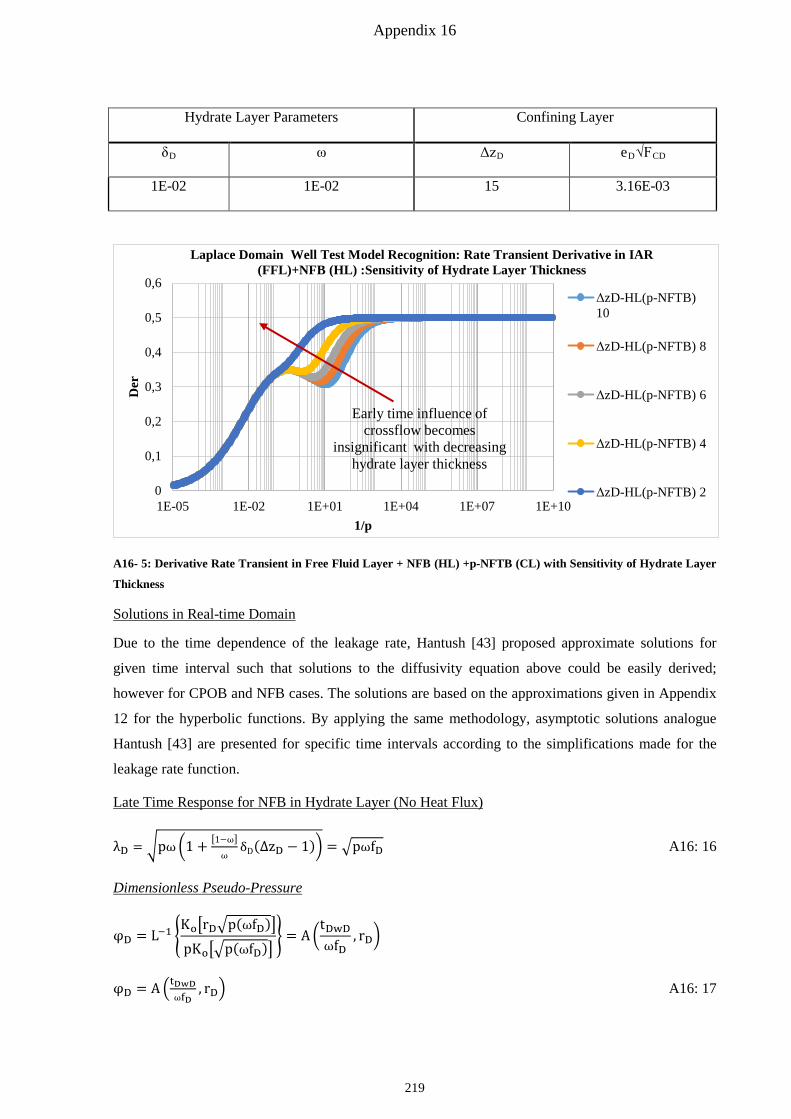
Appendix 16
A16- 5: Derivative Rate Transient in Free Fluid Layer + NFB (HL) +p-NFTB (CL) with Sensitivity of Hydrate Layer
Thickness
Solutions in Real-time Domain
Due to the time dependence of the leakage rate, Hantush [43] proposed approximate solutions for
given time interval such that solutions to the diffusivity equation above could be easily derived;
however for CPOB and NFB cases. The solutions are based on the approximations given in Appendix
12 for the hyperbolic functions. By applying the same methodology, asymptotic solutions analogue
Hantush [43] are presented for specific time intervals according to the simplifications made for the
leakage rate function.
Late Time Response for NFB in Hydrate Layer (No Heat Flux)
λD = �pω�1 + [1−ω]ω
δD(∆zD − 1)� = �pωfD A16: 16
Dimensionless Pseudo-Pressure
φD = L−1 �Ko�rD�p(ωfD)�pKo��p(ωfD)�
� = A �tDwDωfD
, rD�
φD = A �tDwDωfD
, rD� A16: 17
0
0,1
0,2
0,3
0,4
0,5
0,6
1E-05 1E-02 1E+01 1E+04 1E+07 1E+10
Der
1/p
Laplace Domain Well Test Model Recognition: Rate Transient Derivative in IAR (FFL)+NFB (HL) :Sensitivity of Hydrate Layer Thickness
ΔzD-HL(p-NFTB) 10
ΔzD-HL(p-NFTB) 8
ΔzD-HL(p-NFTB) 6
ΔzD-HL(p-NFTB) 4
ΔzD-HL(p-NFTB) 2
Early time influence of crossflow becomes
insignificant with decreasing hydrate layer thickness
Hydrate Layer Parameters Confining Layer
δD ω ΔzD eD√FCD
1E-02 1E-02 15 3.16E-03
219

Appendix 16
For tD = tDwD/(fDωrD²)>500
φD =Ei�
rD2 fDω4tDwD
�
Ei� fDω4tDwD
� A16: 18
Dimensionless Flow rate at Wellbore
mtD = G �tDwDωfD
� A16: 19
Late Time Response for CPOB in Hydrate Layer
λD = �pω�1 +[1−ω]3ω
δD(∆zD − 1)� + δD(∆zD−1) = �pωgD + jD A16: 20
Dimensionless Pseudo-Pressure
φD = Z �tDwDωgD
, rD,�jD� A16: 21
Dimensionless Flow rate at Wellbore
mtD = G �tDwωgD
,�jD� A16: 22
Case 1b: Constant Pressure Outer Boundary Reservoir
General Solution in Laplace Domain
φ�D = c1Io(rDλD) + c2Ko(rDλD)
Boundary conditions
reD φ�D = 0
rD=1 φ�D = 1𝐶𝐶
The coefficients are hence:
c1 = − 1p� Ko(reDλD)�Ko(λD)Io(reDλD)�−Io(λD)Ko(reDλD)� A16: 23
c2 = 1p� Ko(reDλD)Io(reDλD)�Ko(λD)Io(reDλD)�−Io(λD)Ko(reDλD)�
1Ko(reDλD) A16: 24
Dimensionless Pseudo-Pressure
φ�D = 1p�Ko(rDλD)Io(reDλD)−Ko(reDλD)Io(rDλD)
Io(reDλD)Ko(λD)−Io(λD)Ko(reDλD) � A16: 25
Dimensionless Flow rate
m� tD = −rDdφ�DdrD
= −rD1p� 1Io(reDλD)Ko(λD)−Io(λD)Ko(reDλD)
� d�Ko(rDλD)Io(reDλD)−Ko(reDλD)Io(rDλD)�drD
A16: 26
m� tD = rDpλD �
K1(rDλD)Io(reDλD)+Ko(reDλD)I1(rDλD)Io(reDλD)Ko(λD)−Io(λD)Ko(reDλD)
� A16: 27
220
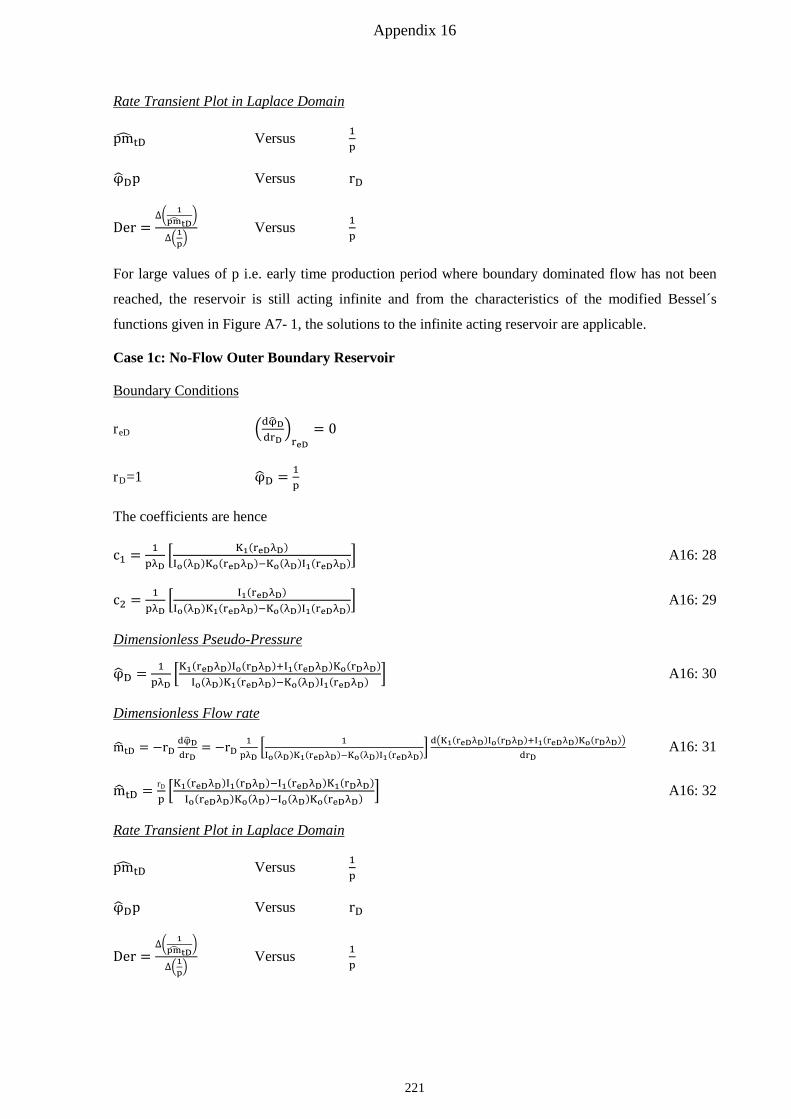
Appendix 16
Rate Transient Plot in Laplace Domain
pm� tD Versus 1p
φ�Dp Versus rD
Der =∆� 1
pm� tD�
∆�1p� Versus 1
p
For large values of p i.e. early time production period where boundary dominated flow has not been
reached, the reservoir is still acting infinite and from the characteristics of the modified Bessel´s
functions given in Figure A7- 1, the solutions to the infinite acting reservoir are applicable.
Case 1c: No-Flow Outer Boundary Reservoir
Boundary Conditions
reD �dφ�DdrD
�reD
= 0
rD=1 φ�D = 1p
The coefficients are hence
c1 = 1pλD
� K1(reDλD)Io(λD)Ko(reDλD)−Ko(λD)I1(reDλD)� A16: 28
c2 = 1pλD
� I1(reDλD)Io(λD)K1(reDλD)−Ko(λD)I1(reDλD)� A16: 29
Dimensionless Pseudo-Pressure
φ�D = 1pλD
�K1(reDλD)Io(rDλD)+I1(reDλD)Ko(rDλD)Io(λD)K1(reDλD)−Ko(λD)I1(reDλD) � A16: 30
Dimensionless Flow rate
m� tD = −rDdφ�DdrD
= −rD1
pλD� 1Io(λD)K1(reDλD)−Ko(λD)I1(reDλD)
� d�K1(reDλD)Io(rDλD)+I1(reDλD)Ko(rDλD)�drD
A16: 31
m� tD = rD
p�K1(reDλD)I1(rDλD)−I1(reDλD)K1(rDλD)
Io(reDλD)Ko(λD)−Io(λD)Ko(reDλD) � A16: 32
Rate Transient Plot in Laplace Domain
pm� tD Versus 1p
φ�Dp Versus rD
Der =∆� 1
pm� tD�
∆�1p� Versus 1
p
221
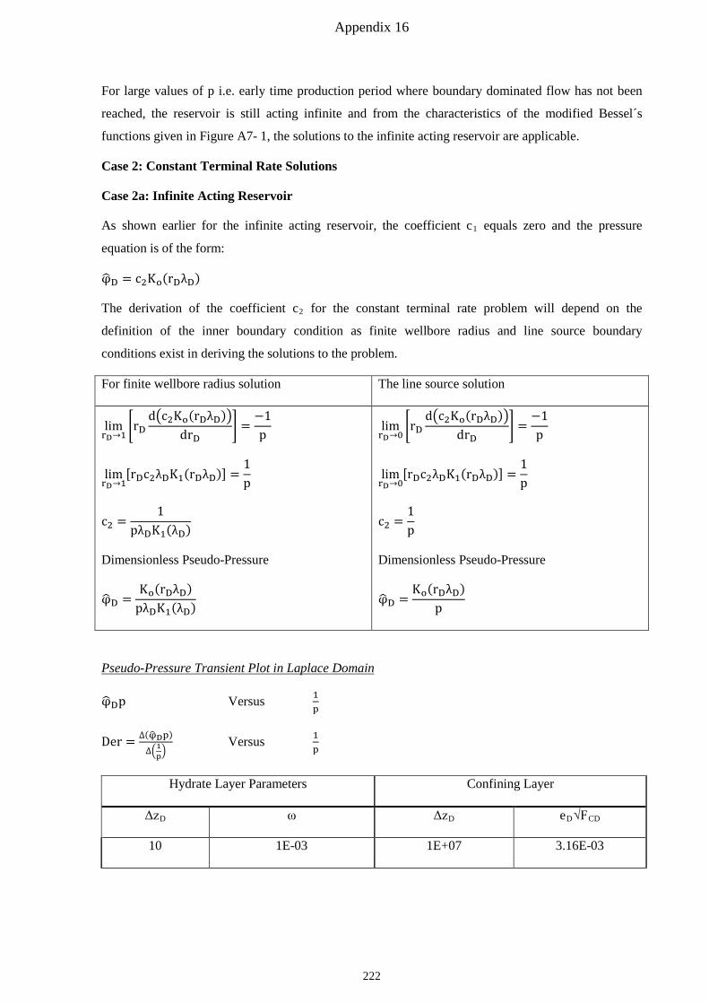
Appendix 16
For large values of p i.e. early time production period where boundary dominated flow has not been
reached, the reservoir is still acting infinite and from the characteristics of the modified Bessel´s
functions given in Figure A7- 1, the solutions to the infinite acting reservoir are applicable.
Case 2: Constant Terminal Rate Solutions
Case 2a: Infinite Acting Reservoir
As shown earlier for the infinite acting reservoir, the coefficient c1 equals zero and the pressure
equation is of the form:
φ�D = c2Ko(rDλD)
The derivation of the coefficient c2 for the constant terminal rate problem will depend on the
definition of the inner boundary condition as finite wellbore radius and line source boundary
conditions exist in deriving the solutions to the problem.
For finite wellbore radius solution The line source solution
limrD→1
�rDd�c2Ko(rDλD)�
drD� =
−1p
limrD→1
[rDc2λDK1(rDλD)] =1p
c2 =1
pλDK1(λD)
Dimensionless Pseudo-Pressure
φ�D =Ko(rDλD)
pλDK1(λD)
limrD→0
�rDd�c2Ko(rDλD)�
drD� =
−1p
limrD→0
[rDc2λDK1(rDλD)] =1p
c2 =1p
Dimensionless Pseudo-Pressure
φ�D =Ko(rDλD)
p
Pseudo-Pressure Transient Plot in Laplace Domain
φ�Dp Versus 1p
Der = ∆(φ�Dp)
∆�1p� Versus 1
p
Hydrate Layer Parameters Confining Layer
ΔzD ω ΔzD eD√FCD
10 1E-03 1E+07 3.16E-03
222
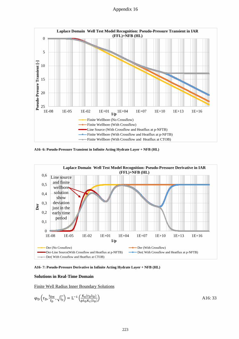
Appendix 16
A16- 6: Pseudo-Pressure Transient in Infinite Acting Hydrate Layer + NFB (HL)
A16- 7: Pseudo-Pressure Derivative in Infinite Acting Hydrate Layer + NFB (HL)
Solutions in Real-Time Domain
Finite Well Radius Inner Boundary Solutions
φD �rD, tDwfD
,�jD� = L−1 � Ko(rDλD)pλDK1(λD)� A16: 33
0
5
10
15
20
251E-08 1E-05 1E-02 1E+01 1E+04 1E+07 1E+10 1E+13 1E+16Ps
eudo
-Pre
sure
Tra
nsie
nt [-
]
1/p
Laplace Domain Well Test Model Recognition: Pseudo-Pressure Transient in IAR (FFL)+NFB (HL)
Finite Wellbore (No Crossflow)Finite Wellbore (With Crossflow)Line Source (With Crossflow and Heatflux at p-NFTB)Finite Wellbore (With Crossflow and Heatflux at p-NFTB)Finite Wellbore (With Crossflow and Heatflux at CTOB)
0
0,1
0,2
0,3
0,4
0,5
0,6
1E-08 1E-05 1E-02 1E+01 1E+04 1E+07 1E+10 1E+13 1E+16
Der
1/p
Laplace Domain Well Test Model Recognition: Pseudo-Pressure Derivative in IAR (FFL)+NFB (HL)
Der (No Crossflow) Der (With Crossflow)Der-Line Source(With Crossflow and Heatflux at p-NFTB) Der( With Crossflow and Heatflux at p-NFTB)Der( With Crossflow and Heatflux at CTOB)
Line source and finite wellbore solution
show deviation just in the early time
period
223
Appendix 16
The solution to the above inverse Laplace can be readily derived by proper application of numerical
inverse Laplace techniques. However, using the line source solution, the solutions presented by [43]
are easily applied. Once more the specific cases of CPOB and NFB are used.
The Line Source Inner Boundary Solutions
φD = L−1 �Ko(rDλD)p
� A16: 34
Early-Time Response for both NFB and CPOB in Hydrate Layer
λD = �pω + δD�[1 − ω]√p = �pω + εD√p A16: 35
φD = H � ωrD2
4tDwD, rDεD
4√ω� A16: 36
Late Time Period for CPOB in Hydrate Layer
λD = �pω�1 +[1−ω]3ω
δD(∆zD − 1)� + δD(∆zD−1) = �pωgD + jD A16: 37
φD = 12
W � rD2
4tDwgD, rD�jD� A16: 38
Late Time Period for NFB in Hydrate Layer
λD = �pω�1 +[1−ω]ω
δD(∆zD − 1)� = �pωfD A16: 39
φD = 12
E1 �ωrD
2
4tDwDfD� A16: 40
Case 2b: Constant Pressure Outer Boundary Reservoir
Boundary Conditions
reD φ�D = 0
rD=1 rDdφ�DdrD
= − 1p
The coefficients are:
c1 = − 1pλD
� Ko(reDλD)K1(λD)Io(reDλD)+I1(λD)Ko(reDλD)� A16: 41
c2 = 1pλD
� Io(reDλD)K1(λD)Io(reDλD)+I1(λD)Ko(reDλD)� A16: 42
Dimensionless Pseudo-Pressure
φ�D = 1pλD
�Ko(rDλD)Io(reDλD)−Ko(reDλD)Io(rDλD)K1(λD)Io(reDλD)+I1(λD)Ko(reDλD) � A16: 43
224

Appendix 16
Pseudo-Pressure Transient Plot in Laplace Domain
φ�Dp Versus 1p
Der = ∆(φ�Dp)
∆�1p� Versus 1
p
For large values of p i.e. early time production period where boundary dominated flow has not been
reached, the reservoir is still acting infinite and from the characteristics of the modified Bessel´s
functions given in Figure A7- 1, the solutions to the infinite acting reservoir are applicable.
Case 2c: No-Flow Outer Boundary in Producing Layer
Boundary Conditions
reD �dφ�DdrD
�reD
= 0
rD=1 rDdφ�DdrD
= − 1p
The coefficients are hence:
c1 = 1pλD
� K1(reDλD)K1(λD)I1(reDλD)−I1(λD)K1(reDλD)� A16: 44
c2 = 1pλD
� I1(reDλD)K1(λD)I1(reDλD)−I1(λD)K1(reDλD)� A16: 45
Dimensionless Pseudo-Pressure
φ�D = 1pλD
�K1(reDλD)Io(rDλD)+I1(reDλD)Ko(rDλD)K1(λD)I1(reDλD)−I1(λD)K1(reDλD) � A16: 46
Pseudo-Pressure Transient Plot in Laplace Domain
φ�Dp Versus 1p
Der = ∆(φ�Dp)
∆�1p� Versus 1
p
For large values of p i.e. early time production period where boundary dominated flow has not been
reached, the reservoir is still acting infinite and from the characteristics of the modified Bessel´s
functions given in Figure A7- 1, the solutions to the infinite acting reservoir are applicable.
225

Appendix 17
Appendix 17: Solutions to the Diffusivity Equation when producing from the Hydrate
Layer
As derived earlier, the diffusivity equation when the hydrate is the producing layer is given by:
∂2φD∂rD
2 + 1rD
∂φD ∂rD
− �∂T𝑝𝑝𝐷𝐷∂z𝐷𝐷
�𝐶𝐶𝐶𝐶𝑝𝑝𝑟𝑟𝐶𝐶𝐶𝐶𝑘𝑘,𝑧𝑧𝐷𝐷=1
− δD(1 + θD) �∂[φD] layer2
∂zD�𝑧𝑧𝐷𝐷=1
= ω� ∂φD∂tDwD
�layer 1
A17: 1
The above equation is given in Laplace domain thus:
∂2φ�D∂rD2
+ 1rD
∂φ�D ∂rD
− QpD� eDφ�D − δD(1 + θD)MiφD� = ωpφ�D A17: 2
∂2φ�D∂rD2
+ 1rD
∂φ�D ∂rD
− λD2φ�D = 0 A17: 3
Where,
λD = �δD(1 + θD)Mi + QpD� eD + ωp A17: 4
It can be noticed that the complex variable λD above is very much different from the case whereby the
reservoir is produced from the free fluid layer. It is important to investigate the influence of hydrate
dissociation when producing from the hydrate layer such that representative reservoir response models
and reservoir parameters for the hydrate layer can be derived.
The equation above can be transformed into the modified Bessel equation and the solution derived
accordingly for which the general solution takes the form:
φ�D = c1Io(rDλD) + c2Ko(rDλD)
A number of combinations of solutions with different boundary conditions can be made to investigate
the reservoir response but however needs care in deriving simplifications for the inverse Laplace
transform. Since just CTOB and p-NFTB have been considered for the confining layer and CPOB and
NFB for the free fluid layer, four different cases can be handled:
• CPOB (FFL) + p-NFTP (CL)
• CPOB (FFL) + CTOB (CL)
• NFB (FFL) + p-NFTP (CL)
• NFB (FFL) + CTOB (CL)
Case 1: Constant Terminal Pressure Solutions
Case 1a: Infinite Acting Reservoir
For the infinite acting system, the coefficient c1 equals zero and by using the inner boundary
condition, the solutions in Laplace domain are given thus:
226

Appendix 17
Inner Boundary
c2 = 1pKo(λD) A17: 5
Dimensionless Pseudo-Pressure
φ�D = Ko(rDλD)pKo(λD) A17: 6
Dimensionless Flow rate
m� tD = − rDλDK1(rDλD)pKo(λD) = rDλDK1(rDλD)
pKo(λD) A17: 7
Rate Transient Plot in Laplace Domain
pm� tD Versus 1p
φ�Dp Versus rD
Der =∆� 1
pm� tD�
∆�1p� Versus 1
p
A17- 1: Derivative Rate Transient in Infinite Acting Hydrate Layer + NFB (HL) + p-NFTB (CL)
0
0,1
0,2
0,3
0,4
0,5
0,6
1E-07 1E-04 1E-01 1E+02 1E+05 1E+08 1E+11 1E+14
Der
1/p
Laplace Domain Well Test Model Recognition: Rate Transient Derivative in Infinite Acting Hydrate Layer
Der (No Crossflow)Der- With Crossflow: NFB (FFL)Der-With Heat: p-NFTB (CL)Der-With Crossflow and Heatflux: p-NFTB (CL) & NFB(FFL)
IARF: Der =0.5
Combined Effects of Heat Influx from confining layer and crossflow from FFL
Diminishing Effects of Heat Influx
Crossflow from FFL still influential
Crossflow from FFL and Heatflux effects become insignificant and reservoir depicts IARF at late time
Free Fluid Layer Parameters Confining Layer
ΔzD ω δD ΔzD eD√FCD
1E+04 1E-04 1E-03 1E+04 3.16E-04
227
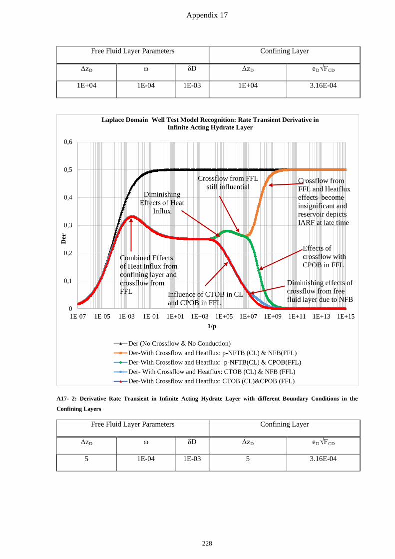
Appendix 17
A17- 2: Derivative Rate Transient in Infinite Acting Hydrate Layer with different Boundary Conditions in the
Confining Layers
0
0,1
0,2
0,3
0,4
0,5
0,6
1E-07 1E-05 1E-03 1E-01 1E+01 1E+03 1E+05 1E+07 1E+09 1E+11 1E+13 1E+15
Der
1/p
Laplace Domain Well Test Model Recognition: Rate Transient Derivative in Infinite Acting Hydrate Layer
Der (No Crossflow & No Conduction)Der-With Crossflow and Heatflux: p-NFTB (CL) & NFB(FFL)Der-With Crossflow and Heatflux: p-NFTB(CL) & CPOB(FFL)Der- With Crossflow and Heatflux: CTOB (CL) & NFB (FFL)Der-With Crossflow and Heatflux: CTOB (CL)&CPOB (FFL)
Combined Effects of Heat Influx from confining layer and crossflow from FFL
Diminishing Effects of Heat
Influx
Crossflow from FFL still influential
Crossflow from FFL and Heatflux effects become insignificant and reservoir depicts IARF at late time
Effects of crossflow with CPOB in FFL
Influence of CTOB in CL and CPOB in FFL
Diminishing effects of crossflow from free fluid layer due to NFB
Free Fluid Layer Parameters Confining Layer
ΔzD ω δD ΔzD eD√FCD
1E+04 1E-04 1E-03 1E+04 3.16E-04
Free Fluid Layer Parameters Confining Layer
ΔzD ω δD ΔzD eD√FCD
5 1E-04 1E-03 5 3.16E-04
228

Appendix 17
A17- 3: Derivative Rate Transient in Infinite Acting Hydrate Layer with different Boundary Conditions in the
Confining Layers
A17- 4: Derivative Rate Transient in Infinite Acting Hydrate Layer with different Boundary Conditions in the Thin
Confining Layers
0
0,1
0,2
0,3
0,4
0,5
0,6
1E-07 1E-05 1E-03 1E-01 1E+01 1E+03 1E+05 1E+07 1E+09 1E+11 1E+13 1E+15
Der
1/p
Laplace Domain Well Test Model Recognition: Rate Transient Derivative in Infinite Acting Hydrate Layer
Der (No Crossflow)Der-With Crossflow and Heatflux: p-NFTB(CL) & NFB(FFL)Der-With Crossflow and Heatflux: p-NFTB (CL) & CPOB(FFL)Der-With Crossflow and Heatflux: CTOB(CL) & NFB(FFL)
Early time response dominated by crossflow effects due to the thin CL and FFL
IARF: Der =0.5
IARF noticeable for reservoirs with no influx at outer boundary
0
0,1
0,2
0,3
0,4
0,5
0,6
1E-07 1E-04 1E-01 1E+02 1E+05 1E+08 1E+11 1E+14 1E+17 1E+20
Der
1/p
Laplace Domain Well Test Model Recognition: Rate Transient Derivative in Infinite Acting Hydrate Layer
Der (No Crossflow)Der( With Crossflow and Heatflux -NFTB & NFB)Der( With Crossflow and Heatflux - NFTB & CPOB)Der( With Crossflow and Heatflux -CTOB& NFB)Der( With Crossflow and Heatflux -CPOB& CTOB)
Early time response dominated by crossflow effects due to the thin CL and FFL
With low heat influx rate, the effects of hydrate dissociation with p-NFTB are not noticeable for thin confining layers and IARF can be perceptible
IARF: Der =0.5
Free Fluid Layer Parameters Confining Layer
ΔzD ω δD ΔzD eD√FCD
5 1E-04 1E-05 5 3.16E-07
229

Appendix 17
Solutions in Real-Time Domain
To obtain the solutions in real time domain, approximations of the leakage rates have to be made as
also seen in Appendix 16.
Usually the effect of CTOB or CPOB overshadows the effects of NFB or p-NFTB all depending on
the influx rate from both layers. We will however consider the following cases.
CPOB in Free Fluid Layer (FFL) and CTOB in Confining Layer (CL)
λD2 = �pω + 𝑉𝑉D��𝑄𝐶𝐶𝐷𝐷� + δD(1+θD)�∆zD,BL−1�
��∆zD,BL − 1��p[1 −ω]�Coth��p[1 −ω]�∆zD,BL − 1��� A17: 8
As given in Appendix 7, the heat influx rate responsible for hydrate dissociation can be quantified and
incorporated in the crossflow model.
λD2 = �pω + �∆zD,TL−1��∆zD,TL−1�
𝑉𝑉D�pFCDCoth��pFCD�∆zD,TL − 1�� + δD(1+θD)�∆zD,BL−1�
��∆zD,BL − 1��p[1−ω]�Coth��p[1 −ω]�∆zD,BL − 1��� A17: 9
NFB in Free Fluid Layer (FFL) and CTOB in Confining Layer (CL)
λD2 = �pω + �∆zD,TL−1��∆zD,TL−1�
𝑉𝑉D�pFCDCoth��pFCD�∆zD,TL − 1�� + δD(1 + θD)��p[1−ω]�tanh��p[1−ω]�∆zD,BL − 1��� A17: 10
Late Time Period for CPOB in FFL and CTOB in CL
λD = �pω�1 + 13ω�𝑉𝑉DFCD�∆zD,TL − 1� + δD(1 + θD)[1−ω]�∆zD,BL − 1��� + � δD(1+θD)
�∆zD,BL−1�+ 𝑈𝑈D
�∆zD,TL−1�� = �pωgD,2 + jD,2 A17: 11
Dimensionless Pseudo-Pressure
φD = Z �tDwDωgD,2
, rD,�jD,2� A17: 12
Dimensionless Flowrate at Wellbore
mtD = G � tDwωgD,2
,�jD,2� A17: 13
Late Time Period for NFB in FFL and CTOB in CL
λD = �pω �1 + 13ω��𝑉𝑉DFCD�∆zD,TL − 1� + 3�δD(1 + θD)(1 −ω)�∆zD,BL − 1�����+ 𝑈𝑈D
�∆zD,TL−1�= �pωfD,2 + YD A17: 14
Dimensionless Pseudo-Pressure
φD = Z �tDwDωfD,2
, rD,�YD� A17: 15
Dimensionless Flow rate at Wellbore
mtD = G �tDwDωfD,2
,�YD� A17: 16
230

Appendix 17
Case 1b: Constant Pressure Outer Boundary Reservoir
Boundary conditions
reD φ�D = 0
rD=1 φ�D = 1𝐶𝐶
The coefficients are hence:
c1 = − 1p� Ko(reDλD)�Ko(λD)Io(reDλD)�−Io(λD)Ko(reDλD)� A17: 17
c2 = 1p� Ko(reDλD)Io(reDλD)�Ko(λD)Io(reDλD)�−Io(λD)Ko(reDλD)�
1Ko(reDλD) A17: 18
Dimensionless Pseudo-Pressure
φ�D = 1p�Ko(rDλD)Io(reDλD)−Ko(reDλD)Io(rDλD)
Io(reDλD)Ko(λD)−Io(λD)Ko(reDλD) � A17: 19
Dimensionless Flow rate
m� tD = rDλDp�K1(rDλD)Io(reDλD)+Ko(reDλD)I1(rDλD)
Io(λD)Ko(reDλD)−Io(reDλD)Ko(λD) � A17: 20
m� tD = λDp�K1(λD)Io(reDλD)+Ko(reDλD)I1(λD)Io(λD)Ko(reDλD)−Io(reDλD)Ko(λD)� A17: 21
Rate Transient Plot in Laplace Domain
pm� tD Versus 1p
φ�Dp Versus rD
Der =∆� 1
pm� tD�
∆�1p� Versus 1
p
For large values of p i.e. early time production period where boundary dominated flow has not been
reached, the reservoir is still acting infinite and from the characteristics of the modified Bessel´s
functions given in Figure A7- 1, the solutions to the infinite acting reservoir are applicable.
Case 1c: No-Flow Outer Boundary in Producing Layer
reD �dφ�DdrD
�reD
= 0
rD=1 φ�D = 1p
The coefficients are hence:
c1 = 1p� K1(reDλD)Io(λD)Ko(reDλD)−Ko(λD)I1(reDλD)� A17: 22
231
Appendix 17
c2 = 1p� I1(reDλD)Io(λD)K1(reDλD)−Ko(λD)I1(reDλD)� A17: 23
Dimensionless Pseudo-Pressure
φ�D = 1p�K1(reDλD)Io(rDλD)+I1(reDλD)Ko(rDλD)
Io(λD)K1(reDλD)−Ko(λD)I1(reDλD) � A17: 24
Dimensionless Flow rate
m� tD = −rDdφ�DdrD
= −rD1p� 1Io(λD)K1(reDλD)−Ko(λD)I1(reDλD)
� d�K1(reDλD)Io(rDλD)+I1(reDλD)Ko(rDλD)�drD
A17: 25
m� tD = 1p
rD �λD[K1(reDλD)I1(rDλD)−I1(reDλD)K1(rDλD)]
Io(λD)Ko(reDλD)−Io(reDλD)Ko(λD)� A17: 26
m� tD = 1p�λD[K1(reDλD)I1(λD)−I1(reDλD)K1(λD)]
Io(λD)Ko(reDλD)−Io(reDλD)Ko(λD)� A17: 27
Rate Transient Plot in Laplace Domain
pm� tD Versus 1p
φ�Dp Versus rD
Der =∆� 1
pm� tD�
∆�1p� Versus 1
p
For large values of p i.e. early time production period where boundary dominated flow has not been
reached, the reservoir is still acting infinite and from the characteristics of the modified Bessel´s
functions given in Figure A7- 1, the solutions to the infinite acting reservoir are applicable.
Case 2: Constant Terminal Rate Solutions
Case 2a: Infinite Acting Reservoir
Inner Boundary Condition
c2 = 1p[λDK1(λD)] A17: 28
Dimensionless Pseudo-Pressure
φ�D = Ko(rDλD)p[λDK1(λD)] A17: 29
Dimensionless Pseudo-Pressure (Line Source)
φ�D = Ko(rDλD)p
A17: 30
Pseudo-Pressure Transient Plot in Laplace Domain
φ�Dp Versus rD
φ�Dp Versus 1p
232
Appendix 17
Der = ∆(φ�Dp)
∆�1p� Versus 1
p
The derivatives given in Case 1a for the rate transient solution are also representative for this case.
Due to the uniqueness of each reservoir response, several reservoir response models could be
generated.
Solutions in Real-Time Domain for Line Source Model
Early-Time Response for No-flow and Constant Pressure Outer Boundary in Crossflow Layer
λD = �pω + �𝑉𝑉D�FCD + δD(1 + θD)�[1 −ω]�√p = �pω + εD,2√p A17: 31
φD = H � ωrD2
4tDwD, rDεD,2
4√ω� A17: 32
Late Time Period for CPOB in FFL and CTOB in CL
λD = �pω�1 +1
3ω�𝑉𝑉DFCD�∆zD,TL − 1� + δD(1 + θD)[1−ω]�∆zD,BL − 1���+ �
δD(1 + θD)�∆zD,BL − 1�
+𝑉𝑉D
�∆zD,TL − 1�� = �pωgD,2 + jD,2
φD = 12
W � rD2
4tDwDωgD,2, rD�jD,2� A17: 33
Late Time Period NFB in FFL and CTOB in CL
λD = �pω �1 + 13ω��𝑉𝑉DFCD�∆zD,TL − 1� + 3�δD(1 + θD)(1 −ω)�∆zD,BL − 1�����+ 𝑈𝑈D
�∆zD,TL−1�= �pωfD,2 + YD A17: 34
φD = 12
W � rD2
4tDwDωfD,2, rD√YD� A17: 35
Case 2b: Constant Outer Boundary Pressure in Producing Layer
Boundary Conditions
reD φ�D = 0
rD=1 rDdφ�DdrD
= − 1p
The coefficients are hence:
c1 = − Ko(reDλD)pλD[K1(λD)Io(reDλD)+Ko(reDλD)I1(λD)] A17: 36
c2 = Io(reDλD)pλD[K1(λD)Io(reDλD)+Ko(reDλD)I1(λD)] A17: 37
Dimensionless Pseudo-Pressure
φ�D = Ko(rDλD)Io(reDλD)−Ko(reDλD)Io(rDλD)pλD[K1(λD)Io(reDλD)+Ko(reDλD)I1(λD)] A17: 38
Pseudo-Pressure Transient Plot in Laplace Domain
φ�Dp Versus rD
233
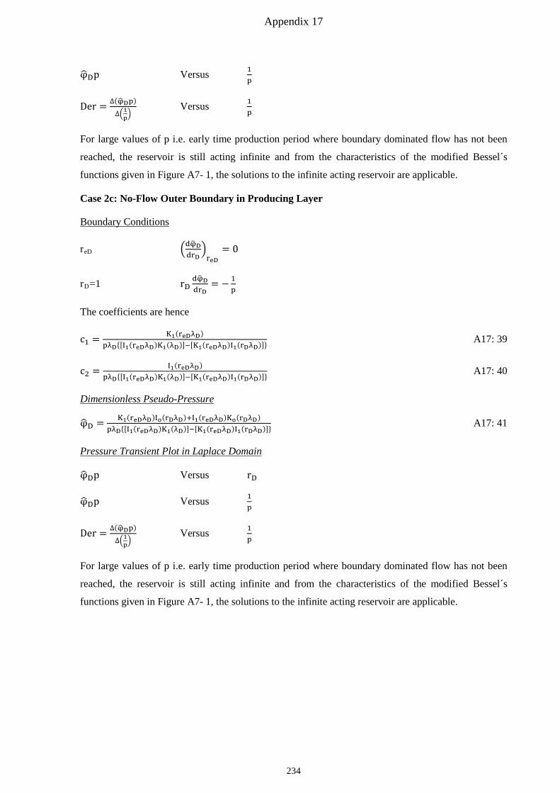
Appendix 17
φ�Dp Versus 1p
Der = ∆(φ�Dp)
∆�1p� Versus 1
p
For large values of p i.e. early time production period where boundary dominated flow has not been
reached, the reservoir is still acting infinite and from the characteristics of the modified Bessel´s
functions given in Figure A7- 1, the solutions to the infinite acting reservoir are applicable.
Case 2c: No-Flow Outer Boundary in Producing Layer
Boundary Conditions
reD �dφ�DdrD
�reD
= 0
rD=1 rDdφ�DdrD
= − 1p
The coefficients are hence
c1 = K1(reDλD)pλD{[I1(reDλD)K1(λD)]−[K1(reDλD)I1(rDλD)]} A17: 39
c2 = I1(reDλD)pλD{[I1(reDλD)K1(λD)]−[K1(reDλD)I1(rDλD)]} A17: 40
Dimensionless Pseudo-Pressure
φ�D = K1(reDλD)Io(rDλD)+I1(reDλD)Ko(rDλD)pλD{[I1(reDλD)K1(λD)]−[K1(reDλD)I1(rDλD)]} A17: 41
Pressure Transient Plot in Laplace Domain
φ�Dp Versus rD
φ�Dp Versus 1p
Der = ∆(φ�Dp)
∆�1p� Versus 1
p
For large values of p i.e. early time production period where boundary dominated flow has not been
reached, the reservoir is still acting infinite and from the characteristics of the modified Bessel´s
functions given in Figure A7- 1, the solutions to the infinite acting reservoir are applicable.
234

Appendix 18
Appendix 18: Reservoir Response Functions
Hantush Functions [43]
Flowing Well Discharge Function for Leaky Aquifers
G(µ,β) = mt(t)2πhk(φi−φwf)
= β K1(β)Ko(β) + 4
π2exp(−µβ2)∫ exp∞
0 (−µx2) x(x2+β2)�Jo2(x)+Yo2(x)�
dx A18: 1
Flowing Well Discharge Function for Non-Leaky Aquifers
G(µ, 0) = mt(t)2πhk(φi−φwf)
= 4π2 ∫
exp�−µx2��Jo2(x)+Yo2(x)�
dxx
∞0 A18: 2
Flowing Well Function for Non-Leaky Aquifers
A(µ,β) = 2πhkmt
[φi − φ(r, t)] = 1 − 2π∫ exp∞
0 (−µx2) [Jo(x)Yo(βx)−Yo(x)Jo(βx)]�Jo2(x)+Yo2(x)�
dxx
A18: 3
Flowing Well Function for Leaky Aquifers
Z(µ,β, τ) = 2πhkmt
[φi − φ(r, t)] = β Ko(τβ)Ko(τ) + 2
πexp(−µτ2)∫ exp(−µx2)
(x2+τ2)[Jo(βx)Yo(x)−Yo(βx)Jo(x)]
�Jo2(x)+Yo2(x)�xdx∞
0 A18: 4
Well Function for Leaky Aquifers
W(µ,β) = 2πhkmt
�φi − φ(r, t)� = ∫ 1𝑥𝑥
exp∞µ �−x − β2
4x�dx A18: 5
W(µ, 0) = E1(µ) = 2πhkmt
�φi − φ(r, t)� = ∫ 1𝑥𝑥
exp∞µ (−x)dx A18: 6
Early Time Well Function for Leaky Aquifers
H(µ,β) = 2πhkmt
�φi − φ(r, t)� = ∫ 𝑈𝑈𝑥𝑥𝐶𝐶(−𝑥𝑥)𝑥𝑥
erfc∞µ � β√µ
�x(𝑥𝑥−𝜇𝜇)�dx A18: 7
Generalized Incomplete Gamma Function [88]
Γ(a,µ; b) = ∫ 1𝑥𝑥1−𝐶𝐶 exp∞
µ �−x− bx�dx A18: 8
dΓ(a,µ;b)dx
= − 1x1−a exp �−x − b
x� A18: 9
Γ(0,µ; b) = ∫ 1𝑥𝑥 exp∞
µ �−x− bx�dx = W(µ,β) A18: 10
Γ(0,µ; 0) = ∫ 1x exp∞
µ (−x)dx = E1(−µ) = −Ei(−µ) A18: 11
235


