FOOTBALL SHOT QUALITY

Visualizing the Quality of Soccer/ Football Shots

Master’s ThesisAndrew RowlinsonAalto University School of BusinessInformation and Service ManagementFall 2020

Aalto University, P.O. BOX 11000, 00076 AALTOwww.aalto.fi

Abstract of master’s thesis

i

Author Andrew Rowlinson

Title of thesis Football shot quality

Degree Master of Science in Economics and Business Administration

Degree programme Information and Service Management

Thesis advisor(s) Timo Kuosmanen

Year of approval 2020 Number of pages 72 Language English

Abstract

Soccer/football differs from other sports because it is relatively low scoring and thereforeunpredictable at a match level. Luck plays its part in a season and underlying results andeven the league tables can lie. Football analytics attempts to strip out some of thisunpredictability and luck so football clubs can make smarter decisions in recruitment,tactics, and strategy.

This thesis aims at answering two questions. First, how to build an expected goals model,which models the probability of scoring from a specific shot. Second, how to visualize theexpected goals metric to give better insight into what makes an effective shot in football.

Keywords football, soccer, expected goals, kernel density estimation

ii

Acknowledgements

Thanks to StatsBomb and Wyscout for sharing the football data and my thesis supervisor

Timo Kuosmanen for the excellent ideas.

Thanks to A&T for being amazing.

This thesis would not have been possible without Matplotlib, NumPy and Pandas. Please

donate to NumFOCUS to support these projects: https://numfocus.org/donate

iii

Table of ContentsAcknowledgements ......................................................................................................... ii

1 Introduction ............................................................................................................. 11.1 Uncertainty ................................................................................................................. 1

1.2 Expected Goals ........................................................................................................... 1

1.3 Research Questions .................................................................................................... 2

1.4 Thesis Structure ......................................................................................................... 2

2 Expected Goals ........................................................................................................ 3

2.1 Expected Goals: Contextual Information. ................................................................. 5

2.2 Expected Goals: Methodology ................................................................................. 12

2.2.1 Logistic Regression ................................................................................................ 12

2.2.2 Decision Tree Methods .......................................................................................... 13

2.3 Expected Goals: Model Calibration......................................................................... 14

2.4 Expected Goals: Validation ...................................................................................... 15

2.5 Expected Goals: Accuracy ....................................................................................... 15

2.6 Expected Goals: Interpretation ............................................................................... 16

3 Kernel Density Estimation .................................................................................... 18

4 Data Sources .......................................................................................................... 224.1 StatsBomb-Open Data.............................................................................................. 22

4.2 Wyscout Soccer Match Event Dataset ..................................................................... 24

4.3 Overlap Between the Datasets ................................................................................. 24

4.4 Combining the StatsBomb and Wyscout Data ........................................................ 28

5 Methods ................................................................................................................. 295.1 Models ...................................................................................................................... 29

5.2 Training .................................................................................................................... 29

5.3 Data........................................................................................................................... 30

6 Findings ................................................................................................................. 356.1 Model Fit .................................................................................................................. 35

6.2 Permutation Importance .......................................................................................... 40

6.3 Partial Dependence Plots ......................................................................................... 41

6.4 Kernel Density Estimation ....................................................................................... 43

6.5 Using Expected Goals to Remove Luck ................................................................... 45

6.6 Shapely Values ......................................................................................................... 49

iv

7 Conclusions ............................................................................................................ 51

References ..................................................................................................................... 54

Appendix A: Features Included in the Logistic Regression Model ............................. 59

Appendix B: Features Included in the Light Gradient Boosting Machine Model ...... 61

v

List of TablesTable 1: Features included in Green’s (2012) Expected Goals model ................................ 6

Table 2: Additional features included in Caley’s (2015) Expected Goals model ................ 7

Table 3: Additional features included in Kullowatz’s (2015) Expected Goals model ......... 8

Table 4: One-hot encoding example ................................................................................ 13

Table 5: Comparison of Scott’s and Silverman’s rules of thumb for kernel density estimation

................................................................................................................................ 21

Table 6:StatsBomb open-data coverage as of 27th June 2020 ........................................... 23

Table 7:Wyscout soccer match event dataset coverage .................................................... 24

Table 8: Train and test datasets ....................................................................................... 34

Table 9: Evaluation metrics ............................................................................................. 35

Table 10:Goalkeeper contribution to shot quality, for goalkeepers with positional data for

200 or more shots .................................................................................................... 50

vi

List of FiguresFigure 1. Distribution of goals in StatsBomb open-data, data accessed on 2020-06-27. ..... 3

Figure 2. Location of goals scored on the pitch (excludes goals scored directly from free-

kicks, corners, or penalties). StatsBomb open-data, data accessed on 2020-06-27 (855

games)....................................................................................................................... 5

Figure 3. Expected Goals: calculating the angles and distances. ........................................ 9

Figure 4. Shot freeze-frame example. Real Madrid versus Liverpool (2018-05-26). Karim

Benzema shot at 5 minutes 11 seconds. ................................................................... 10

Figure 5. Tweet from @Soccermatics on using fake data in Expected Goals models ....... 10

Figure 6. Logistic Regression formula ............................................................................. 12

Figure 7. Partial dependence plot example ...................................................................... 17

Figure 8. Shapely values example ................................................................................... 17

Figure 9. Location of non-penalty goals scored. Scatterplot and histogram. Combined

StatsBomb open-data and Wyscout soccer match event dataset, data accessed on 2020-

06-27 ....................................................................................................................... 18

Figure 10. Location of non-penalty goals scored. Kernel density estimation with bandwidth

chosen via Scott’s Rule of Thumb. Combined StatsBomb open-data and Wyscout

soccer match event dataset, data accessed on 2020-06-27 ........................................ 19

Figure 11. Location of non-penalty goals scored. Kernel density estimation with a bandwidth

of 5. Combined StatsBomb open-data and Wyscout soccer match event dataset, data

accessed on 2020-06-27 .......................................................................................... 20

Figure 12. Shots that are not included in one of the StatsBomb open-data repository or

Wyscout soccer match event dataset for the 100 overlapping games, data accessed

2020-06-27. ............................................................................................................. 25

Figure 13. Percentage point increase in the StatsBomb goal probability when removing shots

that are not in the Wyscout soccer match event dataset for the 100 overlapping games,

data accessed 2020-06-27. ....................................................................................... 25

Figure 14. Shots that are recorded by StatsBomb but are not in the Wyscout data from the

100 overlapping games in the StatsBomb open-data repository and Wyscout soccer

match event dataset, data accessed 2020-06-27. ....................................................... 26

Figure 15. The differences between the location of shots recorded by StatsBomb and

Wyscout within the 100 overlapping games in the StatsBomb open-data repository and

Wyscout soccer match event dataset, data accessed 2020-06-27. ............................. 27

vii

Figure 16. An example of the difference in the location of shots recorded by StatsBomb and

Wyscout. The match is from the FIFA World Cup 2018, Senegal versus Colombia, data

accessed 2020-06-27. .............................................................................................. 27

Figure 17. Location of non-penalty goals scored, combined StatsBomb open-data and

Wyscout soccer match event dataset, data accessed on 2020-06-27. ........................ 28

Figure 18. Probability of scoring from non-penalty shots and potential outliers within the

combined StatsBomb open-data and Wyscout soccer match event dataset, data accessed

on 2020-06-27. ........................................................................................................ 31

Figure 19. Count of non-penalty shots, combined StatsBomb open-data and Wyscout soccer

match event dataset, data accessed on 2020-06-27. .................................................. 32

Figure 20. Location of the fake data points. ..................................................................... 33

Figure 21. Raw probability of scoring from a non-penalty shot with outliers removed and

fake data added inside the penalty area. Combined StatsBomb open-data and Wyscout

soccer match event dataset, data accessed on 2020-06-27. ....................................... 34

Figure 22. Calibration curve showing how well the models fit the real probabilities and the

distribution of the predictions. ................................................................................. 36

Figure 23. The distribution of differences between StatsBomb expected goals predictions

and the light gradient boosting machine model. ....................................................... 37

Figure 24. The average absolute difference between StatsBomb expected goals predictions

and the light gradient boosting machine model. ....................................................... 38

Figure 25. The average expected goals, StatsBomb open-data, accessed 2020-06-27. ...... 39

Figure 26. Permutation importance plot showing the importance of the features for a light

gradient boosting machine model trained on the combined StatsBomb open-data and

Wyscout soccer match event dataset, data accessed on 2020-06-27. ........................ 40

Figure 27. Partial dependence plot showing how location impacts the probability of scoring

a goal by whether or not the assist came from a cross. Light gradient boosting machine

model trained on the combined StatsBomb open-data and Wyscout soccer match event

dataset, data accessed on 2020-06-27....................................................................... 41

Figure 28. Partial dependence plot showing how location impacts the probability of scoring

a goal from a cross by body part used for the shot. Light gradient boosting machine

model trained on the combined StatsBomb open-data and Wyscout soccer match event

dataset, data accessed on 2020-06-27....................................................................... 42

Figure 29. Kernel density estimation. Shot and goal location from the combined StatsBomb

open-data and Wyscout soccer match event dataset, data accessed on 2020-06-27. .. 43

viii

Figure 30. Probabilities of scoring a shot estimated via kernel density estimation from the

combined StatsBomb open-data and Wyscout soccer match event dataset, data accessed

on 2020-06-27. ........................................................................................................ 44

Figure 31. Simulated league table, English Premier League 2017/18 ............................... 46

Figure 32. Simulated league table, France Ligue 1 2017/18 ............................................. 47

Figure 33. Simulated league table, Italy Serie A 2017/18 ................................................ 47

Figure 34. Simulated league table, Germany Bundesliga 2017/18 ................................... 48

Figure 35. Simulated league table, Spain La Liga 2017/18 .............................................. 48

Figure 36. Shapely values showing the contribution of a feature to the chance of scoring

from the light gradient boosting machine model. ..................................................... 49

Figure 37. Partial dependence plot showing the probability of scoring from a kick shot (non-

cross). Light gradient boosting machine model trained on the combined StatsBomb

open-data and Wyscout soccer match event dataset, data accessed on 2020-06-27. .. 52

1

1 Introduction

1.1 Uncertainty

“Football is like chess, but with dice”

Peter Krawietz, Liverpool Football Club coach in Biermann (2019)

Football/soccer differs from other sports because it is relatively low scoring and therefore

unpredictable at a match level. Luck plays its part in a season and underlying results and

even the league tables can lie (Biermann, 2019). Football analytics attempts to strip out some

of this unpredictability and luck so football clubs can make smarter decisions in recruitment,

tactics, and strategy.

According to Anderson and Sally (2014), when comparing the betting odds across

different sports, the bookmakers pick the favourite in football matches less successfully than

in other sports. In football, just over 50% of the favourites win, compared with over 60% in

the popular American team sports. They go on to claim that football is one of the most

uncertain team sports and is “a coin-toss game”, a 50/50 proposition.

Uncertainty in football makes decision making harder. The role of football analytics

is to increase certainty and decrease risk by providing informed analysis.

1.2 Expected Goals

The Expected Goals metric introduced by Sam Green (2012) attempts to strip out the

uncertainty in goal scoring. It measures the shot quality or probability that a shot on average

will score a goal. This means that we can go beyond the actual goals scored, which are

inherently random (Anderson and Sally, 2014) to study on average what should have

happened.

This is useful as football clubs can make smarter decisions on recruitment, tactics, and

strategy. For example, clubs who recruit strikers can look past the randomness of actual

goals scored and identify the underlying shot quality. Thus, clubs can decrease their

recruitment risk by ensuring they do not overpay for a player based on a lucky hot streak of

goals or can also identify players who are unlucky but can create high-quality chances.

2

1.3 Research Questions

This research builds on the current football literature on Expected Goals to make it accessible

and useful to people working in football.

The following questions are studied:

• how to build an Expected Goals model, which measures the quality of shots in

football games?

• how to visualize the Expected Goals model to deliver insight into what makes an

effective shot?

In particular, the visualization question will address how to use kernel density estimators to

explore the shot quality from different match situations.

1.4 Thesis Structure

After the introduction, two sections review the literature on Expected Goals and kernel

density estimation. This is followed by sections explaining the data sources and methods

used for the quantitative part of this thesis, the findings, and key conclusions.

3

2 Expected Goals

“Goals are rare and precious events, ones that clubs spend millions attempting to

guarantee. But they are also random. They can defy explanation and disregard probability.”

(Anderson and Sally, 2014)

Goals are rare in football compared to other sports. The average number of goals scored per

game is 2.66 in the top flights of England, Germany, Spain, Italy, and France between 1993

and 2011 (Anderson and Sally, 2014). While in the National Basketball Association, there

are over 160 points scored per game (Goldsberry, 2019).1

Although football goals are rare and random in isolation, goals are predictable over a

longer time frame. It turns out that football goals are closely fitted by a Poisson model

(Maher, 1982). According to Anderson and Sally (2014), we can predict the distribution of

goals per game by taking the average number of goals in a game and applying the Poisson

distribution.

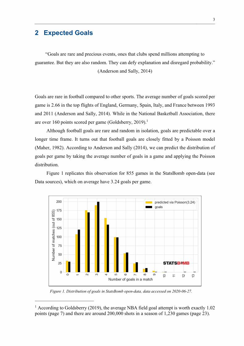
Figure 1 replicates this observation for 855 games in the StatsBomb open-data (see

Data sources), which on average have 3.24 goals per game.

Figure 1. Distribution of goals in StatsBomb open-data, data accessed on 2020-06-27.

1 According to Goldsberry (2019), the average NBA field goal attempt is worth exactly 1.02points (page 7) and there are around 200,000 shots in a season of 1,230 games (page 23).

4

Figure 1 shows that the distribution of goals per game predicted by a Poisson

distribution is very similar to the actual goals per game from the StatsBomb open-data. This

means although a single goal is seemingly rare and random, over longer periods a logical

pattern appears within the data.

However, as football is a low scoring game, singular and rare events such as goals

have a much greater impact in football than in sports like basketball (Biermann, 2019). Luck,

therefore, plays a role as individual events have a greater impact. This luck means that the

underlying results and even the league tables may lie. Schoenfeld (2019) explains that

Liverpool Football Club hired Jürgen Klopp as their manager, partially based on evidence

showing that Klopp had been unlucky during his previous season managing Borussia

Dortmund. According to Liverpool’s analysis, Borussia Dortmund deserved to be placed

five places higher in the final German Bundesliga table. This gave reassurance to Liverpool

that Jürgen Klopp was managing at a higher level than suggested by the Bundesliga table in

his final season at Borussia Dortmund.

“Luck plays a much greater role in football that we would like to admit: it’s even

quantifiable. If Jürgen Klopp had known as much, he might never become coach of

Liverpool FC ” (Biermann, 2019)

We can start to quantify the chance of scoring from a given position using event data

collected from shots (Biermann, 2019). Figure 2 shows a figure with the proportion of goals

coming from specific locations on the pitch from over 20 thousand open-play shots within

the 855 games in the StatsBomb open-data (see Data sources).

The figure shows mostly what one would expect to see, most goals are scored closer

to the goal. However, this figure lacks contextual information. For example, we know that

shots which are assisted from crosses are harder to convert than shots from other situations

(Knutson, 2016), but this is not considered in the figure.

5

Figure 2. Location of goals scored on the pitch (excludes goals scored directly from free-kicks, corners, or

penalties). StatsBomb open-data, data accessed on 2020-06-27 (855 games).

2.1 Expected Goals: Contextual Information.

“If I shoot there, I've got a six in ten chance of scoring,” [Teddy] Sheringham explains. “If

I roll the ball to Shearer, he's got an eight in ten chance. That is instinctively weighed up in

a split second” (Rudd, 2020)

To capture the contextual information that football players evaluate when deciding whether

to shoot from a specific position, Sam Green introduced the Expected Goals metric. This is

often abbreviated as xG. The idea of the Expected Goals metric is to measure the shot chance

quality (Green, 2012).

6

According to Gregory (2017), the Expected Goals model introduced by Green uses the

following contextual information:

Table 1: Features included in Green’s (2012) Expected Goals model

Feature Description

Distance Distance to the middle of the goal (the mid-point between

the goalposts)

Visible angle of the goal The angle formed between the shot location and the two

goal posts

Passage of play One of open play, direct free kick, set play, corner kick,

assisted, and throw-in

Assist type One of a long ball, cross, through ball, danger-zone pass,

and pull-back

Post take-on/ dribble Whether the shot follows a previous attempt to beat a player

Rebound Whether the shot follows a previous shot that has

rebounded

Header Whether the shot came off the attacking player’s head

1 versus 1 A shot where there is just one defensive player to score past

Big chance A situation where a player should reasonably be expected

to score, usually in a one on one scenario or from very close

range when the ball has a clear path to goal and there is low

to moderate pressure on the shooter. (Opta, 2018)

7

The contextual information the model uses is typically referred to as features in

machine learning (Müller & Guido, 2017). Feature engineering is a crucial step in machine

learning, which transforms and extracts new features from the existing features (Zheng and

Casari, 2018). Caley (2015) adds some additional features and uses feature engineering in

their Expected Goal model:

Table 2: Additional features included in Caley’s (2015) Expected Goals model

Feature Description

Fast break An attempt created after the defensive quickly turn defence

into attack winning the ball in their own half (Opta, 2018)

Counterattack An engineered feature to capture counterattacks that are not

marked as fast breaks by Opta’s coders. “These are actions

that begin with an open play turnover of possession, in

which the attacking team moves steadily forward to the

goal without recirculating the ball.”

Established possession An engineered feature that is defined as “an attack that

involves at least five completed passes in the attacking half

without the ball being forced back into the defensive zone.”

Relative angle to the goal The angle to the nearest post. If a player is in a central

position, the angle is 1. If a player is at a 45-degree angle

to the nearest post, the angle is 0.5.

Interaction between the

distance and angle

An interaction feature, which captures interactions between

distance and angle to the goal (Zheng and Casari, 2018).

This is the distance to the goal multiplied by the relative

angle to the goal.

Dribble distance The distance a player has dribbled before taking the shot.

Error Whether the shot follows an error by another player.

Body part The body part used to take the shot

Game state The game state is a feature that describes whether the team

taking the shot is losing, drawing, or winning the match at

the time of the shot.

League A feature for the league, for example, the Bundesliga or the

English Premier League.

8

Caley (2015) creates separate models for different match situations to reflect the

varying difficulty of taking shots. This allows the significant features in each model to be

studied. Caley creates six models for:

• regular shots

• shots from a direct free kick

• headed shots from a cross

• headed shots not from a cross

• non-headed shots from a cross

• shots following a dribble from the keeper thus the goalkeeper is not in goal when

the shot is taken

Caley notes their disappointment about including a feature for the league (e.g.

Bundesliga) in the model, which appears to capture real differences in the shot selection and

play between the leagues. While the game state is found to have a small effect for regular

shots, which Caley believes captures the unaccounted differences in defensive pressure

applied by teams trailing or leading a match.

Kullowatz (2015) built on the existing models and creates some additional features:

Table 3: Additional features included in Kullowatz’s (2015) Expected Goals model

Feature Description

Log distance The logarithm of the distance to the centre of the goal

Width of the goal mouth

available to the shooter

The angle to the middle of the goal (American Soccer). See

the first diagram in Figure 3 for the calculation. This is

converted to yards using an unexplained quadratic function.

9

The amount of goal visible to the shot taker is a common feature in Expected Goal

models. Sumpter (2017) describe the importance of the shooting angle when taking a shot:

“the more goal you see when you shoot, the better your chance of scoring.” However, the

distances and angles can be calculated by referencing different positions on the pitch, such

as the nearest/furthest goal post or the middle of the goal. Figure 3 shows two methods to

calculate the angles. The method for calculating the visible angle to the goalposts is taken

from Sumpter (2017).

Figure 3. Expected Goals: calculating the angles and distances.

As Caley (2015) noted, features for the game state (e.g. winning) and league appear to

be capturing latent factors that cannot be observed in the event data, such as the amount of

defensive pressure asserted at the time the shot is taken. In 2018, the sports data provider

StatsBomb announced that they are collecting pressure events. According to Will Gurpinar-

Morgan (2018), pressure events are events that are triggered when a player enters within a

5-yard radius to the player in possession. Also, Ted Knutson (2018), announced that

StatsBomb collects information on the position of the players at the time a shot is taken,

known as shot freeze frames. According to Ted Knutson, using shot freeze frames leads to

less biased Expected Goals models as the model can account for pressure on the shot taker

and situations that lead to more blocked shots. Figure 4 demonstrates a single example of

this shot freeze frame data.

10

Figure 4. Shot freeze-frame example. Real Madrid versus Liverpool (2018-05-26). Karim Benzema shot at 5

minutes 11 seconds.

Using the shot freeze-frame and pressure data, additional features can be engineered

to capture the defensive pressure. For example, David Sumpter (2020a) explains that the

number of players within the range of the visible angle to the goalposts or the position of the

nearest player to the shot taker can be good features.

A final technique to increase the accuracy of an Expected Goals model is to include

football knowledge in the model by creating fake data points (@Soccermatics). As the event

data is observed data, it is often lacking in areas that players do not take many shots. David

Sumpter explains that inserting engineered data helps to overcome the limitations of the

event data.

Figure 5. Tweet from @Soccermatics on using fake data in Expected Goals models

11

The last distinction for Expected Goals models is that they typically do not use data

from after the point the player strikes the ball (Goodman, 2018). This means the model does

not include information after the shot, such as the direction, speed, and angle the ball is

heading. Typically, they also do not include information on the player taking the shot,

although examples such as Kwiatkowski (2017) exist. This is because Expected Goals

models are meant to estimate “how the average player or team would perform in a similar

situation” (FBref). Expected Goals, therefore, provide a baseline for measuring the amount

a player outperforms the average player in a similar situation but does not account for a

player’s skill or shot selection.

Gelade (2017) also states that Expected Goals are better predictors of goals scored than

goals conceded. For measuring a goalkeepers’ ability, another metric exists called Post-Shot

Expected Goals (Goodman, 2018). This includes information after the shot is taken and helps

to evaluate the probability of a goal given a shot’s placement, an important factor for

evaluating goalkeepers.

12

2.2 Expected Goals: Methodology

The Expected Goals metric is a classic supervised learning problem. A classification model

is tasked with classifying whether a shot is a goal or not, given the contextual information at

the time the shot was taken. Green (2012), Caley (2015), Kullowatz (2015) all use logistic

regression methodology to calculate the original Expected Goals metric, but any

classification model would be appropriate for this type of problem, such as random forests

or other decision tree methods.

2.2.1 Logistic Regression

“Logistic regression is a simple, linear classifier. […] It takes a weighted combination of

the input features, and passes it through a sigmoid function, which smoothly maps any real

number to a number between 0 and 1” (Zheng and Casari, 2018)

The formula for logistic regression is (Müller, A. & Guido, 2016):

ŷ (predictions) = (w0 * x0) + (w1 * x1) + ... + (wn * xn) + b

where wi are the weights for the ith feature

xi is the ith feature

b is an interecept term

Figure 6. Logistic Regression formula

A logistic classifier generally predicts “the positive class if the sigmoid output is

greater than 0.5, and the negative class otherwise” (Zheng and Casari, 2018). The machine

learning problem is to find a weight combination that minimizes the error, which in the case

of logistic regression is the logistic loss.

One factor to consider with logistic regression is how to represent the categorical

features, such as the shot assist type, which can take one of several options such as long ball

or cross. The categorical features do not make sense as a weighted linear combination

because that would imply a linear relationship between the categories. This is generally

solved with one-hot encoding (Zheng and Casari, 2018) where each category is assigned a

single feature. If the one-hot encoded feature is 1 then it implies that the observation belongs

to this category, if it is 0 it implies that the observation does not belong to this category. An

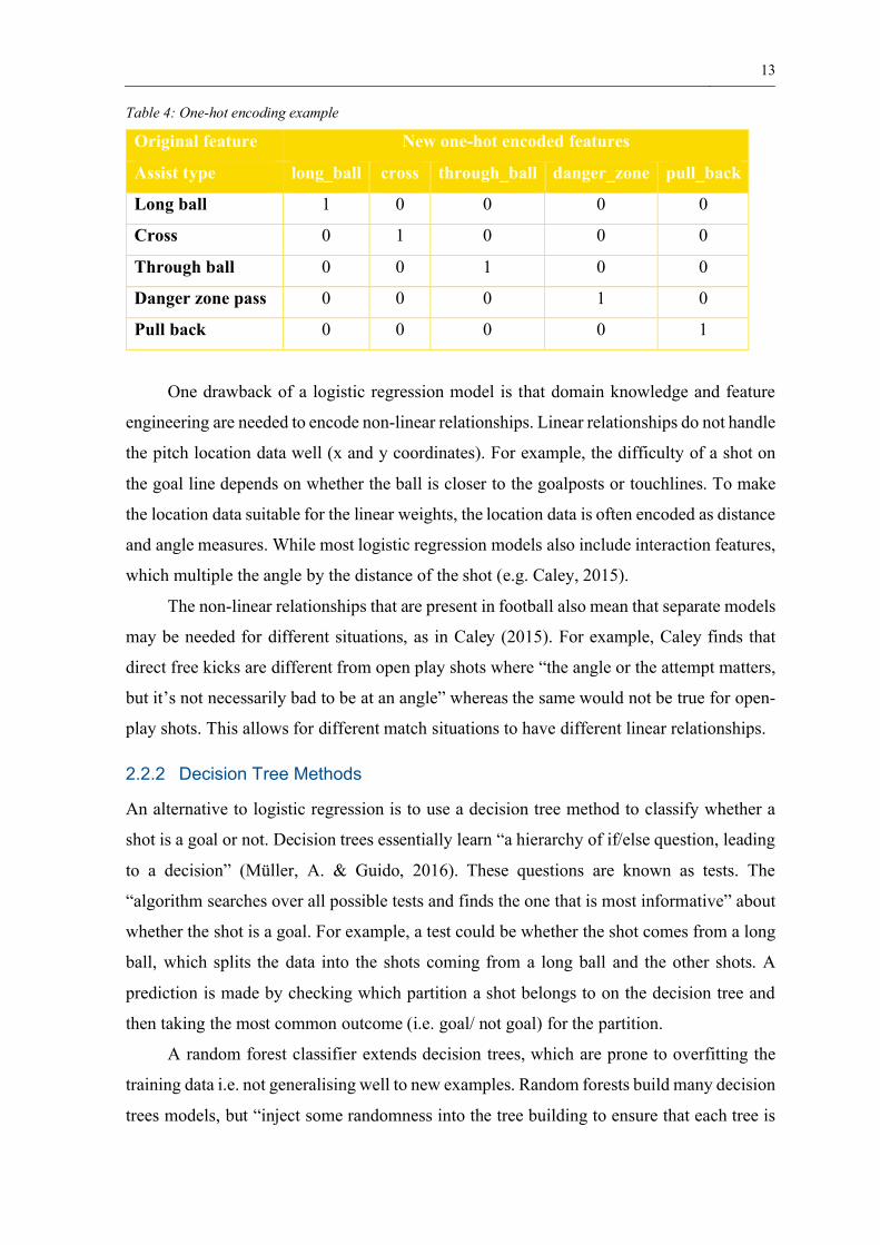
example of one-hot encoding the assist type feature is represented in Table 4.

13

Table 4: One-hot encoding example

Original feature New one-hot encoded features

Assist type long_ball cross through_ball danger_zone pull_back

Long ball 1 0 0 0 0

Cross 0 1 0 0 0

Through ball 0 0 1 0 0

Danger zone pass 0 0 0 1 0

Pull back 0 0 0 0 1

One drawback of a logistic regression model is that domain knowledge and feature

engineering are needed to encode non-linear relationships. Linear relationships do not handle

the pitch location data well (x and y coordinates). For example, the difficulty of a shot on

the goal line depends on whether the ball is closer to the goalposts or touchlines. To make

the location data suitable for the linear weights, the location data is often encoded as distance

and angle measures. While most logistic regression models also include interaction features,

which multiple the angle by the distance of the shot (e.g. Caley, 2015).

The non-linear relationships that are present in football also mean that separate models

may be needed for different situations, as in Caley (2015). For example, Caley finds that

direct free kicks are different from open play shots where “the angle or the attempt matters,

but it’s not necessarily bad to be at an angle” whereas the same would not be true for open-

play shots. This allows for different match situations to have different linear relationships.

2.2.2 Decision Tree Methods

An alternative to logistic regression is to use a decision tree method to classify whether a

shot is a goal or not. Decision trees essentially learn “a hierarchy of if/else question, leading

to a decision” (Müller, A. & Guido, 2016). These questions are known as tests. The

“algorithm searches over all possible tests and finds the one that is most informative” about

whether the shot is a goal. For example, a test could be whether the shot comes from a long

ball, which splits the data into the shots coming from a long ball and the other shots. A

prediction is made by checking which partition a shot belongs to on the decision tree and

then taking the most common outcome (i.e. goal/ not goal) for the partition.

A random forest classifier extends decision trees, which are prone to overfitting the

training data i.e. not generalising well to new examples. Random forests build many decision

trees models, but “inject some randomness into the tree building to ensure that each tree is

14

different” (Müller, A. & Guido, 2016). A prediction is then made by taking the average of

the decision trees in the random forest. A random forest estimator is usually better than a

single decision tree because its variance is reduced (scikit-learn, a).

Another extension to decision trees is boosted decision trees. These extend decision

trees by building several weak decision trees sequentially with each one aiming to reduce

the bias of the last decision tree (scikit-learn, a). A prediction is then made by taking the sum

of the decision tree predictions in the ensemble.

The main benefits of decision tree methods over logistic regression are:

• they can handle categorical features without using one-hot encoding to encode

features since several tests can combine to split a categorical feature

• they can model non-linear relationships (e.g. shot location data) without any feature

engineering because the trees can naturally create interactions by combining several

tests to partition the data (e.g. headed shots from a cross)

2.3 Expected Goals: Model Calibration

“A model is called calibrated if the reported uncertainty actually matches how correct it

is—in a calibrated model, a prediction made with 70% certainty would be correct 70% of

the time.” (Müller & Guido, 2017)

To be of any use to football practitioners the Expected Goals model must be well-

calibrated. That is a prediction giving an Expected Goal value of 70% likely must result in

a goal 70% of the time. This is vital so that professionals believe the results from the model.

The main advantage of using logistic regression for Expected Goals is that that by default

logistic regression returns well-calibrated predictions whereas random forests and boosted

decision trees have difficulty making predictions near 0 and 1 (scikit-learn, b). This means

that an extra step is often needed for random forests to calibrate the model, so it returns

probabilities.

Niculescu- Mizil and Rich Caruana (2005) find that calibrated decision tree methods

work well for predicting probabilities. They test two methods: Platt Scaling, which is

effective when the dataset is small, and Isotonic Regression, which is more powerful when

there is sufficient data. The Platt Scaling method passes the outputs through a sigmoid

15

function to get probabilities in the range 0 to 1, whereas Isotonic Regression learns a

mapping function. For both methods, an independent dataset is needed to calibrate the model

and reduce bias.

The Brier score is a metric typically used to measure how well the model is calibrated.

The score ranges between 0 and 1 with lower values representing better-calibrated models.

It measures the mean squared difference between the predicted probability and the actual

outcome (scikit-learn, c).

2.4 Expected Goals: Validation

The Expected Goals model also must generalise well to new shots that the model has not

seen. This is because we are interested in making predictions of the probability of scoring

from new shots.

A common machine learning method to evaluate generalisation performance is to use,

k-fold cross-validation, where k is usually 5 or 10 (Müller & Guido, 2017). In k-fold

validation, the data is partitioned into k-folds of equal size. Then k models are built

sequentially, each time one of the k-folds is selected as a validation set and the rest of the

data is used to train the model. The accuracy of the k validation folds is then reported in the

cross-validation routine, e.g. the mean accuracy for the k-folds.

Typically, in machine learning, we are interested in ensuring the model generalises

well to new examples. We use cross-validation to select parameters of the model that

improve its generalisation performance, e.g. parameters that use shallow rather than deep

decision trees so they do not overfit. An important part of machine learning is to select a

suitable metric to optimise.

2.5 Expected Goals: Accuracy

Gelade (2017) evaluates several Expected Goals models and identifies two suitable metrics

for evaluating model performance:

• McFadden’s pseudo-R2: which compares the model to a null model which

predicts the same prediction for every shot.

• Receiver operating characteristics (ROC) curves, which plot the true positive

rate against the false-positive rate, at different threshold settings for the classifier,

such as predicting a goal if the prediction is more than 0.5. The Area Under the

16

(ROC) Curve (AUC) then gives the probability that the Expected Goals model will

rank a randomly chosen goal higher than a randomly chosen non-goal shot.

Gelade states that these measures “are particularly useful because they are bench-

marked at both ends. The lower end represents a model that performs no better than chance

while the top end represents a model that delivers completely accurate predictions.”

2.6 Expected Goals: Interpretation

The Expected Goals metric provides the probability of scoring from a specific shot. But

often we want to go beyond this and understand why a model made the prediction. This helps

us understand what makes a shot low quality and how we could improve the overall quality

of chances.

An advantage of logistic regression is that it is more easily interpretable than some

decision tree methods. The logistic regression weights can be interpreted in terms of odds

ratios (Eye and Mun, 2013), with direct interpretation in real-life. While decision trees are

also interpretable because of their strict if/else tests, the ensemble methods, which have

higher generalisation ability, do not have a straightforward interpretation.

Hall and Gill (2018) define local and global interpretability for machine learning

models. Global interpretability helps to explain the approximate effect of an input feature

for the entire model, while local interpretations help to explain the prediction for a single

shot.

17

A partial dependence plot provides global interpretability. It shows the average way

the shot quality changes based on the values of one or two input features, such as the x and

y coordinates of the shot (Hall and Gill, 2018). This can help explain how the shot quality

changes depending on the shot location, while other effects are averaged out. Figure 7 shows

a partial dependence plot for the number of players in the visible angle to goal, it shows that

the probability of scoring a goal is around 3 to 4 percentage points lower when two or more

players are within the visible angle to the goal.

Figure 7. Partial dependence plot example

Shapely values then provide local interpretability. Shapely values create an

explanation for each shot based on the contributions of the input features. For example, each

input feature, such as the assist type, is assigned a value showing how much it increases or

decreases the probability of scoring a goal. In the example in figure 8, the largest negative

contribution is because the shot is far from the goal line, as the x coordinate is 80.5 out of

105. While the largest positive contribution is because the shot is central, as the y coordinate

is 38.7 out of 68. Intuitively this makes sense as shots far away from the goal line are harder

to convert, while central shots are easier than shots closer to the touchlines, which have a

narrower angle to the goal.

Figure 8. Shapely values example

18

3 Kernel Density Estimation

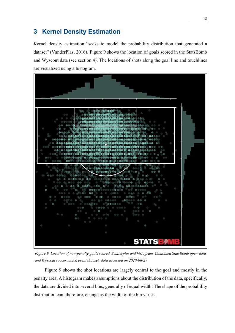
Kernel density estimation “seeks to model the probability distribution that generated a

dataset” (VanderPlas, 2016). Figure 9 shows the location of goals scored in the StatsBomb

and Wyscout data (see section 4). The locations of shots along the goal line and touchlines

are visualized using a histogram.

Figure 9. Location of non-penalty goals scored. Scatterplot and histogram. Combined StatsBomb open-data

and Wyscout soccer match event dataset, data accessed on 2020-06-27

Figure 9 shows the shot locations are largely central to the goal and mostly in the

penalty area. A histogram makes assumptions about the distribution of the data, specifically,

the data are divided into several bins, generally of equal width. The shape of the probability

distribution can, therefore, change as the width of the bin varies.

19

A kernel density estimator attempts to smooth the probability distribution, so it more

accurately reflects the true shape of the probability distribution and the data it represents.

(VanderPlas, 2016).

A shot map is again shown in Figure 10, but this time replacing the data points with

the probability distributions from a kernel density estimator.

Figure 10. Location of non-penalty goals scored. Kernel density estimation with bandwidth chosen via Scott’s

Rule of Thumb. Combined StatsBomb open-data and Wyscout soccer match event dataset, data accessed on

2020-06-27

The kernel density estimator replaces the data points with a kernel, such as a Gaussian

normal distribution kernel. The kernels are then normalized and summed for each point to

create the overall probability distribution. When using kernel density estimation, the key

20

parameters are the type of kernel and the size of the kernel, known as bandwidth

(VanderPlas, 2016).

The bandwidth can dramatically change the appearance of the probability distribution.

Figure 11 shows the same shot data with a gaussian kernel and bandwidth of 5. The

bandwidth of this kernel is too large, so the probability distribution is a poor fit of the actual

data – it under fits the data.

Figure 11. Location of non-penalty goals scored. Kernel density estimation with a bandwidth of 5. Combined

StatsBomb open-data and Wyscout soccer match event dataset, data accessed on 2020-06-27

There are several rules of thumb for setting the size of the bandwidth. Two popular

rules are Silverman (1986) and Scott (2015). Scott’s rule of thumb was first published in

1992. The rules of thumb are very similar, but Scott’s rule of thumb produces slightly larger

bandwidths. The difference between the methods is a single scalar value, which is used as a

21

multiplier in the calculation. In Scott’s method, the scalar value is 1.059 (statsmodel, a) and

in Silverman’s rule of thumb, the scalar value is 0.9 (statsmodel, b), according to the

statsmodel Python implementation.

Table 5: Comparison of Scott’s and Silverman’s rules of thumb for kernel density estimation

Scott’s rule of thumb

(statsmodel, a)

Silverman’s rule of thumb

(statsmodel, b)

0.9 * A * n-0.2 1.059 * 0.9 * A * n-0.2

Where:

A = minimum(standard_deviation(values, degrees_of_freedom=1),

interquartile_range(x)/1.349)

n = number of observations

Jake VanderPlas (2016) explains the importance of selecting the bandwidth so that the

estimator does not underfit the data (too wide a bandwidth) or overfit the data (too narrow a

bandwidth). VanderPlas illustrates using a machine learning approach, cross-validation, as

an alternative to the statistical rules of thumb. The cross-validation approach seeks to

identify the bandwidth that maximizes the log-likelihood.

The cross-validation approach typically uses k-fold validation (see section 2.4) or in

the cases of small datasets leave-one-out cross-validation. Leave-one-out cross-validation is

a special case of k-fold validation where each data point is used once as a validation set,

while the remaining data is used for training. This is also equivalent to k-fold validation with

the number of folds (k) set to the number of data points.

22

4 Data Sources

There are two main types of football data:

• event data, which records actions on the pitch. These are typically on-the-ball

actions, such as passes, shots and tackles. But occasionally cover off-the-ball-actions,

such as pressure events (Gurpinar-Morgan, 2018).

• tracking data, which records the positions of the players, referees, and the ball at

regular intervals.

This thesis uses event data from two sources the StatsBomb open-data repository 2 and

the Wyscout soccer match event dataset (Pappalardo and Massucco, 2019), as described in

Pappalardo, Cintia, Rossi et al. (2019).

In this thesis, event data is used to calculate and visualize the Expected Goals metric.

Also, the location of players at the time of the shot is utilised to capture information on the

pressure on the shot taker and the potential for a blocked shot (see Figure 4).

The disadvantage of using event data is that it does not cover many off-the-ball events.

Off-the-ball events are important because players spend most of the time without the ball

(Davies, 2013). For example, within the StatsBomb open-data, the most common event type

is a pass, which players make on average 42 times per match, or on average once every two

minutes. Since the event data is generally on-ball events, the event data does not cover key

information such as space creation and the ability for defenders to close the space available

for the team attacking.

4.1 StatsBomb-Open Data

There are 855 games in the StatsBomb data as of 27th June 2020. The coverage of the

dataset is shown in Table 6.

The data are biased since most of the data are for matches involving FC Barcelona,

which account for 33% of the total shots in the dataset. While just over 2,000 of the

approximate 21,800 shots belong to one player, Lionel Messi. This is a limitation as the

Expected Goals metric is supposed to measure the ability of the average player. However,

the dataset is skewed towards shots by a player who is generally considered as one of the

best players in modern history.

2 Available at https://github.com/statsbomb/open-data

23

Table 6:StatsBomb open-data coverage as of 27th June 2020

CompetitionNumber

of gamesSeasons Coverage

Men’s La Liga 452 15 seasons from

2004/05 to 2017/19

Games featuring Lionel

Messi, who plays for FC

Barcelona.

FA Women's Super

League

195 2018/19

2019//20

All

Men’s FIFA World

Cup

64 2018 All

Women’s FIFA

World Cup

52 2019 All

National Women's

Soccer League

46 2018 A few selected games.

English Premier

League

32 2003/04 Only games involving

Arsenal Football Club. In

the invincible season in

which they lost no games.

Missing six matches from

the season

UEFA Champions

League

14 14 finals: 2003/2004,

2004/2005,

2006/2007, and 11

finals between

2008/09 and 2018/19

UEFA Champions League

finals.

24

4.2 Wyscout Soccer Match Event Dataset

There are 1941 games in the Wyscout soccer match event dataset as of 27th June 2020. The

coverage of the dataset is in Table 7.

Table 7:Wyscout soccer match event dataset coverage

CompetitionNumber

of gamesSeasons

French Ligue 1 380 2017/18

English Premier League 380 2017/18

Italian Serie A 380 2017/18

Spanish La Liga 380 2017/18

German Bundesliga 306 2017/18

Men’s FIFA World Cup 64 2018

Men’s UEFA Euro 51 2016

4.3 Overlap Between the Datasets

The StatsBomb and Wyscout data overlap in 100 games. The overlap is 64 games from the

Men’s FIFA World Cup 2018 and 34 FC Barcelona games in the 2017/18 La Liga season in

which Lionel Messi played.

Event data is usually manually recorded by professionals who watch the game and

record the events. We can study the overlapping games to identify any differences in how

the data providers record shot attempts. In the 100 overlapping games, Wyscout records

fewer non-penalty shot attempts (2,420) than StatsBomb (2,604).

Figure 12 shows the location of the non-penalty shot events, which are recorded

differently by the two data providers. It shows that StatsBomb has greater coverage with

around 200 shots (about 2 every game) more than Wyscout data.

25

Figure 12. Shots that are not included in one of the StatsBomb open-data repository or Wyscout soccer match

event dataset for the 100 overlapping games, data accessed 2020-06-27.

As Wyscout reports the same amount of goals but fewer shot attempts, the raw goal

probabilities are higher for Wyscout data compared to StatsBomb data. Figure 13 shows the

percentage point increase in the raw goal probabilities for the StatsBomb data, after

removing the shot attempts which are not counted by Wyscout.

Figure 13. Percentage point increase in the StatsBomb goal probability when removing shots that are not in

the Wyscout soccer match event dataset for the 100 overlapping games, data accessed 2020-06-27.

26

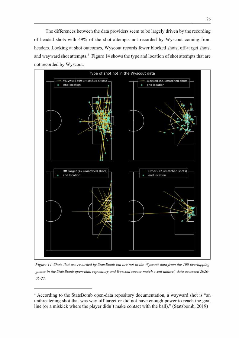
The differences between the data providers seem to be largely driven by the recording

of headed shots with 49% of the shot attempts not recorded by Wyscout coming from

headers. Looking at shot outcomes, Wyscout records fewer blocked shots, off-target shots,

and wayward shot attempts.3 Figure 14 shows the type and location of shot attempts that are

not recorded by Wyscout.

Figure 14. Shots that are recorded by StatsBomb but are not in the Wyscout data from the 100 overlapping

games in the StatsBomb open-data repository and Wyscout soccer match event dataset, data accessed 2020-

06-27.

3 According to the StatsBomb open-data repository documentation, a wayward shot is “anunthreatening shot that was way off target or did not have enough power to reach the goalline (or a miskick where the player didn’t make contact with the ball).” (Statsbomb, 2019)

27

We can also look at how the location information for non-penalty shots is recorded.

These are generally quite similar, with most shot locations within five metres of each other

when comparing the data providers. Figure 15 shows the distribution of the shot location

differences in the 100 overlapping games and Figure 16 shows an example for one game in

the men’s FIFA World Cup.

Figure 15. The differences between the location of shots recorded by StatsBomb and Wyscout within the 100

overlapping games in the StatsBomb open-data repository and Wyscout soccer match event dataset, data

accessed 2020-06-27.

Figure 16. An example of the difference in the location of shots recorded by StatsBomb and Wyscout. The

match is from the FIFA World Cup 2018, Senegal versus Colombia, data accessed 2020-06-27.

28

4.4 Combining the StatsBomb and Wyscout Data

Despite the differences in the datasets, an Expected Goals model will likely perform better

when it has more data points, as there will likely be more variety in the shot types (Müller

& Guido, 2017).

In this thesis, the StatsBomb open-data and Wyscout soccer match dataset have been

combined to create a single dataset of non-penalty shots. The Wyscout data are removed in

the case of overlapping data, since the StatsBomb data has richer information, such as the

location of players at the time of the shot. After, removing the overlapping data, there are

2,696 games, 64,396 shots and 6,854 goals. Figure 17 shows a heatmap of the number of

non-penalty shots by location for the combined Wyscout and StatsBomb dataset.

Figure 17. Location of non-penalty goals scored, combined StatsBomb open-data and Wyscout soccer match

event dataset, data accessed on 2020-06-27.

29

5 Methods

5.1 Models

I create two Expected Goals models in this thesis:

• a logistic regression baseline model

• a light gradient boosting machine model, which is based on boosted decision trees

(Ke, Meng, Finley, Wang, Chen, Ma, Ye, Liu, 2017)

The published models show logistic regression works relatively well in the context of

Expected Goals (Green, 2012; Caley, 2015; Kullowatz, 2015). Logistic regression, therefore,

provides a good baseline to evaluate whether the light gradient boosting machine model

works well.

The main reason for using an additional decision tree-based model is to build an

Expected Goals model using raw shot location data (x and y coordinates), rather than

engineered features such as angle and distance to the goal. This means that the Expected

Goals predictions can be interpreted by referencing real positions on the pitch, rather than

the more abstract distances and angles. This is not possible with logistic regression models

without losing accuracy as logistic regression predictions are a linear combination of weights

so factors with interactions, such as x and y coordinates, are more difficult to encode with

linear weights (see section 2.2.1).

5.2 Training

The models are trained on the training dataset of over 51 thousand shots. The features used

to train the models are included in Appendices A and B, while the dependent variable is a

Boolean column for whether a goal was scored.

The data for the logistic regression model is split into two modelling problems:

• shots coming from a pass assist

• shots which do not come from a pass assist, such as shots coming from a direct

freekick, rebound, or clearance

The data are split because there are more features for shots that come from a pass, such

as a type of assisting pass and distance the player carried the ball before taking the shot,

which is not present for other types of shots. Logistic regression requires that all the features

have non-missing values. Thus, splitting the data into two separate modelling problems

30

means that the missing values for passes do not need to be imputed for the non-pass assisted

shots.

In total three models are trained, two logistic regression models and one light gradient

boosting machine model. The models are validated and optimised using 5-fold cross-

validation on the training dataset (scikit-learn, d).

The light gradient boosting machine model is calibrated using isotonic regression so

that the predictions produce well-calibrated probabilities on the calibration dataset using 3-

fold cross-validation. The calibration cross-validation loop is nested inside the 5-fold cross-

validation loop to maximize the use of the available training data.

Finally, the accuracy metrics are reported on the test dataset containing around 13,000

shots.

5.3 Data

There are 855 games in the StatsBomb open-data and 1841 games in the Wyscout data after

the overlapping games have been removed. A shot dataset is created from these games

containing over 64 thousand non-penalty shots. Shots that have come directly from corners

are also excluded. There are some areas of the football pitch that have fewer shot attempts

where it is generally harder to score. In these areas, there are some outliers where goals have

been scored from relatively few shots. Caley (2013) suggests that these anomalies are usually

where the goalkeeper has been caught out of position or come from a fortunate cross that

has eluded all the players in the box and ended as a goal.

To make the model fit better some of these outliers have been removed. First, the data

have been binned into a grid of approximately 2-metre squares. Then I remove 227 shots

from squares with fewer than 20 shots and a probability of scoring 8 per cent or more. The

removed shot outliers are marked in red in figure 18.

31

Figure 18. Probability of scoring from non-penalty shots and potential outliers within the combined

StatsBomb open-data and Wyscout soccer match event dataset, data accessed on 2020-06-27.

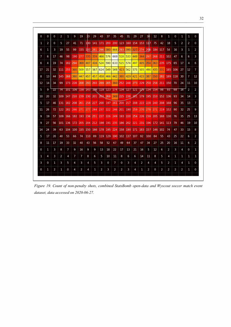
The white grid squares in figure 18 are areas where there are no shots at all. However,

there are also large sections of the penalty area with tight angles to the goal where are

relatively few shots in the dataset. These are shown in the darker colours in figure 19.

32

Figure 19. Count of non-penalty shots, combined StatsBomb open-data and Wyscout soccer match event

dataset, data accessed on 2020-06-27.

33

A thousand fake data points have been created in parts of these areas to encode our football

knowledge that these areas are difficult to score from (@sumpter). The shots are created

from grid squares with fewer than 100 shots within the penalty area, which are not next to

the goalmouth. The fake shots in the grid squares touching the goal line are all marked as

non-goals, while shots further out are marked as a goal with probability 4.1%, which is the

average probability of scoring from shots within this area in the dataset. The fake data points

are shown in figure 20. The other features for the fake shots, such as the assist type, are

randomly sampled from shots from within the grid cells used to create the fake data.

Figure 20. Location of the fake data points.

34

After removing outliers and adding the fake data, the resulting data has smoother

probabilities, which are shown in figure 21.

Figure 21. Raw probability of scoring from a non-penalty shot with outliers removed and fake data added

inside the penalty area. Combined StatsBomb open-data and Wyscout soccer match event dataset, data

accessed on 2020-06-27.

The remaining shots are then randomly split into a training (80%) and test dataset

(20%). I use stratified random sampling, so the proportion of goals scored is consistent

across the datasets (10.6%). Table 8 below shows the number of real shots, and goals scored

in each split: A further 1000 fake goals are also added to the training dataset when training

the light gradient boosting machine model.

Table 8: Train and test datasets

Dataset Number of shots Number of goals

Train 51,335 5,443

Test 12,834 1,361

35

6 Findings

6.1 Model Fit

Overall, the light gradient boosting machine model provides a slightly better fit of shot

quality according to the McFadden’s pseudo-R-squared measure in Table 9, with a similar

scored for the other evaluation metrics. The results are in the same range as the values

reported in Garry Gelade’s comparison of expected goals metrics for standard models

(2017). Although the evaluation metrics are slightly below another model, which uses an

additional “big chance” feature, which Opta uses to code shots that a player should

reasonably be expected to score (Opta, 2018). A model using this feature improves on the

ROC AUC metric (0.807) and McFadden R-squared (0.22). This type of feature is not

available in either the Wyscout or StatsBomb datasets.

Table 9: Evaluation metrics

MetricType Logistic

regression

Light gradient

boosting machine

Brier scoreLower better

(see section 2.3)

0.0815 0.0804

Receiver Operating

Characteristic Area

Under the Curve

(ROC AUC)

Higher better

(see section 2.5)

0.7867 0.7851

McFadden’s pseudo

R-squared

Higher better

(see section 2.5)

0.1648 0.1699

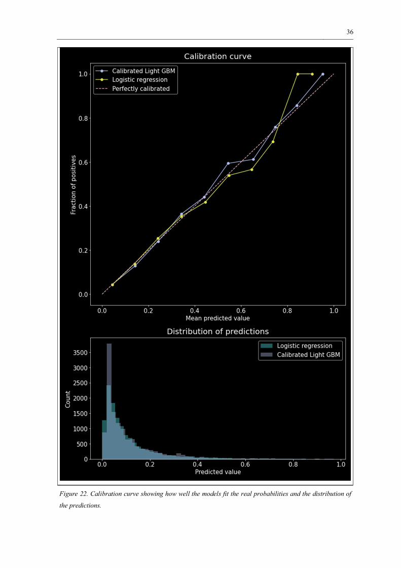
The light gradient boosting machine model has been calibrated with isotonic

regression. The Brier score (Table 9) and the calibration curve (Figure 22) show that the

predicted probabilities are well-calibrated. A well-calibrated model means that the predicted

probabilities can be interpreted as a measure of shot quality. The calibration curve is also

known as the reliability curve (Niculescu-Mizil & Caruana, 2005). The calibration curve

bins the data, in this case into 10 bins, and compares the predicted probabilities of goals in

the bin to the actual fraction of goals in the bin. A perfectly calibrated model results in the

predicted probabilities equaling the actual fraction, which is the 45-degree line in figure 22.

36

Figure 22. Calibration curve showing how well the models fit the real probabilities and the distribution of

the predictions.

37

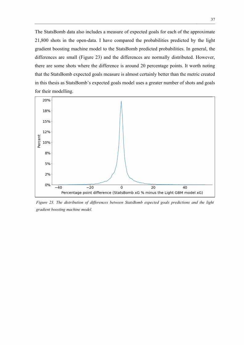
The StatsBomb data also includes a measure of expected goals for each of the approximate

21,800 shots in the open-data. I have compared the probabilities predicted by the light

gradient boosting machine model to the StatsBomb predicted probabilities. In general, the

differences are small (Figure 23) and the differences are normally distributed. However,

there are some shots where the difference is around 20 percentage points. It worth noting

that the StatsBomb expected goals measure is almost certainly better than the metric created

in this thesis as StatsBomb’s expected goals model uses a greater number of shots and goals

for their modelling.

Figure 23. The distribution of differences between StatsBomb expected goals predictions and the light

gradient boosting machine model.

38

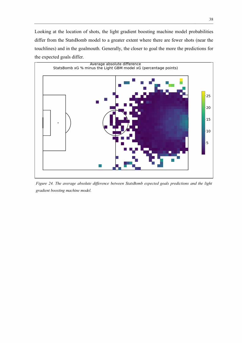
Looking at the location of shots, the light gradient boosting machine model probabilities

differ from the StatsBomb model to a greater extent where there are fewer shots (near the

touchlines) and in the goalmouth. Generally, the closer to goal the more the predictions for

the expected goals differ.

Figure 24. The average absolute difference between StatsBomb expected goals predictions and the light

gradient boosting machine model.

39

Figure 25 explores the average expected goals by the location on the pitch. This shows that

when the ball is 25 metres away from the goal line the probability of scoring drops to 2% or

lower. While the probability of scoring is 10% or higher in the rectangle inside the penalty

area and 10 metres on either side of the goal centre. The figure uses the StatsBomb expected

goal metric, as this is more accurate closer to the goal line since it is based on a greater

number of shots.

Figure 25. The average expected goals, StatsBomb open-data, accessed 2020-06-27.

40

6.2 Permutation Importance

Importance measures show the importance of a feature to the predictions of the model (Hall

and Gill (2018). Permutation importance achieves this by randomly shuffling features and

reporting the change in the model’s score (Breiman, 2001). Figure 26 shows a box plot with

the features ordered by their permutation importance. By a clear distance, the location of the

shot is the most important driver of the probability of scoring a goal. This is followed by the

body part used to take the shot, the goalkeeper position, and the number of players within

the angle to goal. Intuitively these all make sense and follow what we might expect to see

from a good fitting model.

Figure 26. Permutation importance plot showing the importance of the features for a light gradient boosting

machine model trained on the combined StatsBomb open-data and Wyscout soccer match event dataset, data

accessed on 2020-06-27.

41

6.3 Partial Dependence Plots

As the shot location is the most important factor for determining shot quality, we can look

at this in more detail using partial dependence plots. These allow us to look at how location

impacts the shot quality while averaging out the effects of the other features (Hall and Gill,

2018). Figure 27 compares kick shots from crosses to non-crosses and follows the

observations of Ted Knutson (2016) that crosses are harder to convert than non-crosses.

Figure 27. Partial dependence plot showing how location impacts the probability of scoring a goal by

whether or not the assist came from a cross. Light gradient boosting machine model trained on the combined

StatsBomb open-data and Wyscout soccer match event dataset, data accessed on 2020-06-27.

42

While further breaking down crosses by the body part used to take the shot, we can

also show that non-kick shots from crosses, which are typically headers, are far harder to

convert than kick-shots from crosses, as also observed by Ted Knutson (2016).

Figure 28. Partial dependence plot showing how location impacts the probability of scoring a goal from a

cross by body part used for the shot. Light gradient boosting machine model trained on the combined

StatsBomb open-data and Wyscout soccer match event dataset, data accessed on 2020-06-27.

43

6.4 Kernel Density Estimation

I have trained two kernel density estimators using 10-fold cross-validation for shots and

goals scored. The figure below shows that players tend to take shots in central locations, just

in front of the penalty spot. While a few shots are taken from relatively poor pitch positions

outside the penalty, where fewer goals are scored. In this figure, the probabilities are higher

when the colour is lighter.

Figure 29. Kernel density estimation. Shot and goal location from the combined StatsBomb open-data and

Wyscout soccer match event dataset, data accessed on 2020-06-27.

44

I use these two kernel density estimators of the shot and goal location to estimate the

probability of scoring by shot location, shown in figure 30. This is potentially a simpler

method of showing how shot location impacts the chance quality than the partial dependence

plots.

I use the following method to estimate the goal probabilities:

• train two kernel density estimators for the shots and goals using the same

bandwidth, I used a bandwidth of around 1.44.

• score the probability density of shots and goals using the estimators for fixed

locations on the pitch, for example, I use a grid of 0.25 meter squared

• divide the probability density of a goal by the probability density of a shot and

multiple by the ratio of goals to shots in the data. The ratio of goals to shots is around

0.106 (10.6%) for the combined StatsBomb and Wyscout data used in this thesis.

Figure 30. Probabilities of scoring a shot estimated via kernel density estimation from the combined

StatsBomb open-data and Wyscout soccer match event dataset, data accessed on 2020-06-27.

This figure presents an intuitive view of how shot quality is impacted by the location

of the shot. Shots within the six-yard box and close to the goal have a high chance, 30% or

higher of converting. Shots within the circle to the penalty spot, which is around 11 metres

from the goal centre, have a 17% chance or higher of being converted. While shots within

the penalty arc, which is around 22 metres from the goal centre, have an 8% or higher chance

of being converted to goals except for tight angles to the goal.

45

6.5 Using Expected Goals to Remove Luck

Football is a game of relatively few goals and therefore luck or the variance in the conversion

of goals can have a high impact in a single game or even over a whole season. Using expected

goals, we can strip out the luck element and estimate how many goals the team would have

been expected to score based on the quality of chances created in a game.

We can then simulate the probabilities of winning, losing, or drawing a game based on

the predicted quality of shots in the game. A simulation reruns a match many times and

estimates the number of goals based on the quality of shot chances within a game, so if a

chance has 10% chance quality it will be converted in 10% of the simulated games. A team

can only score once from a single playing sequence in real-life so for this analysis shots are

first grouped so any shots occurring within 15 seconds of another shot are in the same group.

Only a single goal is allowed for each shot group during a simulated game. Shots taken from

penalties are given an expected shot quality of 76%, which is the value given to penalties in

the StatsBomb data.

Using the goals from the simulated games, we can assign three points for a win and

one point for a draw in each of the simulated games. We can then estimate the distribution

of points a team would be expected to accumulate based on the simulated games and the

distribution of their expected positions in the league table. The simulation approach strips

out the luck or variance for single shots and more accurately reflects where a team should

be positioned in the table given the quality of the shots they generate and concede.

In this thesis, I simulate 10,000 seasons for each of the leagues within the Wyscout

data. The data are for the men’s topflight games in the French, English, Italian, Spanish, and

German leagues in the 2017/18 season. When teams are tied on points, their positions are

decided by the actual league position during that season. There is a simplification as the rules

for deciding the position for tied teams depend on the league, such as goal difference or

head-to-head results.

A common football cliché is goals change games. As goals are relatively rare in

football, a team which scores from a low-quality shot may deliberately play more

conservatively to conserve their lead and create fewer shot opportunities. Thus, a drawback

of the simulation approach is that we do not know how the teams would react differently in

the absence of a lucky goal.

46

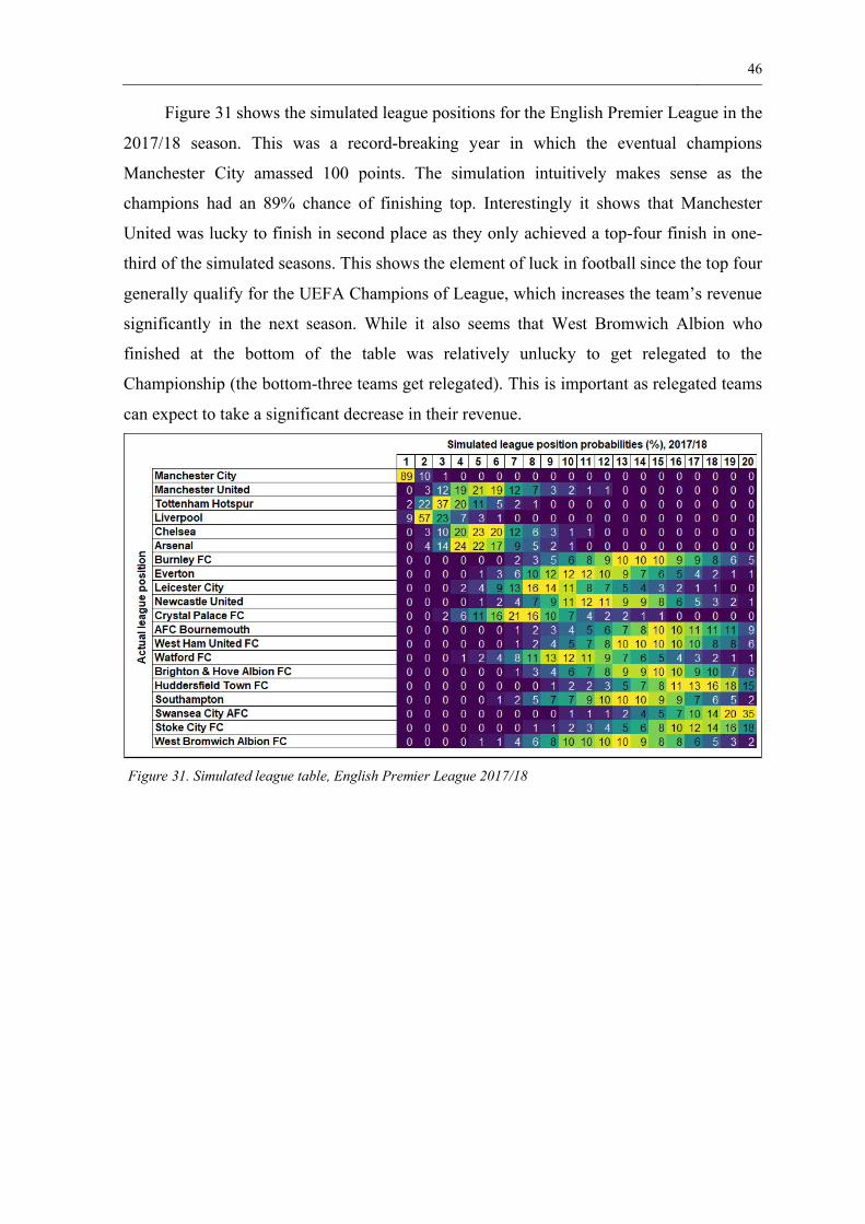
Figure 31 shows the simulated league positions for the English Premier League in the

2017/18 season. This was a record-breaking year in which the eventual champions

Manchester City amassed 100 points. The simulation intuitively makes sense as the

champions had an 89% chance of finishing top. Interestingly it shows that Manchester

United was lucky to finish in second place as they only achieved a top-four finish in one-

third of the simulated seasons. This shows the element of luck in football since the top four

generally qualify for the UEFA Champions of League, which increases the team’s revenue

significantly in the next season. While it also seems that West Bromwich Albion who

finished at the bottom of the table was relatively unlucky to get relegated to the

Championship (the bottom-three teams get relegated). This is important as relegated teams

can expect to take a significant decrease in their revenue.

Figure 31. Simulated league table, English Premier League 2017/18

47

France’s Ligue 1 is similar to the English Premier League as Paris Saint-Germain

dominated the league with an 89% chance of finishing top.

Figure 32. Simulated league table, France Ligue 1 2017/18

While in Italy’s Serie A, Atalanta B.C. was extremely unlucky to finish in seventh place and

even had a 20% chance of winning the league, a higher probability than the eventual

champions Juventus.

Figure 33. Simulated league table, Italy Serie A 2017/18

48

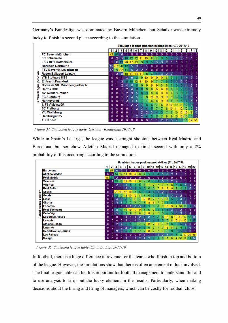
Germany’s Bundesliga was dominated by Bayern München, but Schalke was extremely

lucky to finish in second place according to the simulation.

Figure 34. Simulated league table, Germany Bundesliga 2017/18

While in Spain’s La Liga, the league was a straight shootout between Real Madrid and

Barcelona, but somehow Atlético Madrid managed to finish second with only a 2%

probability of this occurring according to the simulation.

Figure 35. Simulated league table, Spain La Liga 2017/18

In football, there is a huge difference in revenue for the teams who finish in top and bottom

of the league. However, the simulations show that there is often an element of luck involved.

The final league table can lie. It is important for football management to understand this and

to use analysis to strip out the lucky element in the results. Particularly, when making

decisions about the hiring and firing of managers, which can be costly for football clubs.

49

6.6 Shapely Values

We can also use Shapely values to interpret for a specific shot which features contribute to

shot quality. This can be used to identify shots where the goalkeeper position increases the

chance of a goal by a large margin, such as this shot attempts in figure 36. This may be used

for tactical analysis and recruitment decisions to help identify potential weaknesses.

Figure 36. Shapely values showing the contribution of a feature to the chance of scoring from the light

gradient boosting machine model.

50

Using the contributions of the goalkeeper positioning, we can identify how positioning

impacts the chance quality in aggregate. Table 10 below ranks goalkeepers by the number

of times their positioning decreased the shot quality by 1 percentage point. For example, a 1

percentage point decrease could decrease a shot chance from 10% to 9%. The table is for

goalkeepers with at least 200 shots in the StatsBomb data. As the data for men’s competition

matches are biased towards the games featuring Barcelona, it is difficult to draw conclusions.

However, for the women’s competition, this could potentially provide insight on

goalkeeper’s positioning that could be used for recruitment or coaching purposes.

Table 10:Goalkeeper contribution to shot quality, for goalkeepers with positional data for 200 or more shotsPlayer Name Competition gender % good goalkeeper

position (decrease in

shot quality by 1+

percentage points)

% bad goalkeeper

position (increase in

shot quality by 5+

percentage points)

Shots faced

Sophie Baggaley female 48 5 592

Ellie Roebuck female 45 4 357

Claudio Bravo male 44 6 684

Megan Walsh female 42 6 626

Grace Moloney female 41 12 336

Gorka Iraizoz male 41 12 256

Marc-André ter Stegen male 40 6 1122

Rebecca Spencer female 40 5 387

Carlos Kameni male 40 10 233

Kirstie Levell female 40 2 263

José Manuel Pinto male 38 8 225

Diego Alves male 37 8 278

Keylor Navas male 36 11 213

Marie Hourihan female 36 5 213

Víctor Valdés male 35 9 2054

Anke Preuß female 35 3 339

Iker Casillas male 34 14 222

Hannah Hampton female 32 9 260

Jens Lehmann male 32 6 319

51

7 Conclusions

The appetite to explain and deliver insights into the game of soccer/ football is growing. For

example, Bundesliga recently announced they will display match facts, such as expected

goals, during the live broadcast of the German topflight matches (Bundesliga, 2020).

Although expected goals models are used widely to explain the results of individual

games and seasons. There has been less public-facing research using interpretability

techniques can deliver insights, which this thesis aims to supplement.

In this thesis, I have covered two research questions:

• how to build an Expected Goals model, which measures the quality of shots in

football games?

• how to visualize the Expected Goals model to deliver insight into what makes an

effective shot?

I build an expected goals model that uses raw pitch coordinates rather than engineered

features, such as distance to the goal. This achieves similar accuracy to other published

methods at an aggregate level but differs at a shot level due to the relatively small amount

of data used in the modelling.

I then present several visualization methods to explain the quality of the shots by the

pitch location using partial dependence plots and kernel density estimation. I also use

Shapely values to explain how features contribute towards the shot quality and use

simulation to explain how luck can influence the league tables. This shows that players still

take shots from relatively low scoring situations, such as from 25 metres where the chance

of scoring can be as small as 2%.

One way to teach players about shot quality is to paint shot rings on the training pitch

representing the chance of scoring from a position, as suggested in Knutson (2016). Figure

37 presents how this could look using the results of the partial dependence plot for the non-

cross kick shots.

52

Figure 37. Partial dependence plot showing the probability of scoring from a kick shot (non-cross). Light

gradient boosting machine model trained on the combined StatsBomb open-data and Wyscout soccer match

event dataset, data accessed on 2020-06-27.

Basketball has already been influenced by analytics with the result that the players are

taking a greater proportion of shots from long range, known as 3 pointers, as they are more

valuable than other shots (Goldsberry, 2019). There is also a recent trend in football to take

fewer low-value shots from outside the penalty box. However, shots from outside the penalty

box still accounted for 39% of all shots in the English Premier League 2018/19 season (Bate,

2018). Over time, I expect these low-value, non-optimal, shots will decline further as

analytics plays a greater role in decision making. Players should look to progress the ball

into areas with higher shot quality rather than taking opportunities with just a 2% chance of

success.

The limitation of this thesis is the relatively small amount of shots used for the

modelling. After the location of the shot, many of the most important features tend to be the

location of other players, such as goalkeeper. Unfortunately, this information was only

available for around 20 thousand of the 60 thousand shots. With additional data, the model

would achieve a better fit and more closely resemble the actual probabilities of scoring from

53

a specific shot. In addition, it is likely that combining data from two providers (Wyscout and

StatsBomb) is sub-optimal as the data come from different distributions (Davis and

Robberechts, 2020). With additional data, these shortcomings could be addressed, and the

model would provide improved estimates of shot quality in areas of the pitch where there

are fewer shots, for example, directly in front of the goal.

This thesis has only explained shot quality. Shot quality is a small part of the analytics

puzzle and the creation of shots is equally as important. Other work has attempted to attribute

the creation of shots to specific events in the game. Some examples of this research include:

• Sarah Rudd (2011) use of Markov models to value how much a player contributes

to creating good goal scoring opportunities

• The Valuing Actions by Estimating Probabilities (VAEP) framework, which values

player events while accounting for the circumstances of the event (Decroos, Bransen,

Van Haaren and Davis, 2019)

• The Expected Threat (xT) framework, which estimates the expected threat from

attacking options (Singh, 2019).

• Expected Goal Chain (xGChain), which attributes the expected goal metric to

specific shots in the possession chain that led to the shot (Lawrence, 2018)

• The Possession Value Framework, which attempts to model the expected outcome

and value for each event on the pitch (Fernández, Bornn and Cervone, 2019)

• Goals Added (GA), which attempts to value each defending or attacking event on

the pitch in terms of goals added and conceded (Doyle-Davis, 2020)

The research on Goals Added is an important development, which seeks to attribute

values to both defending and attacking events. This is an area of research that should be

explored further so that players and tactics can be evaluated against their overall impact on

the game, not just the attacking element of football.

54

References

@Soccermatics. “The point of the fake data is two-fold. It allows you to include

things you know that are impossible (put players never do because its

impossible) and then you can push the non-linear terms to really understand

how the probability of success is shaped.” Twitter, 13 May. 2020, 6:50 p.m.,

https://twitter.com/Soccermatics/status/1260598182624575490.

American Soccer. “What are expected Goals?”

https://www.americansocceranalysis.com/explanation. Accessed 23 May 2020.

Anderson, Chris. & Sally, David. The Numbers Game. Why Everything You Know About

Football is Wrong, 2nd edition, Penguin, Great Britain, 2014.

Bate, Adam “Do long shots work? Andre Schurrle and Ruben Neves buck the trend” Sky

Sports, 2018, https://www.skysports.com/football/news/11661/11540002/do-long-

shots-work-andre-schurrle-and-ruben-neves-buck-the-trend. Accessed 3 July 2020

Bundesliga “DFL and Amazon Web Services to provide new real-time match analysis”,

2020, https://www.bundesliga.com/en/bundesliga/news/new-real-time-match-

analysis-dfl-and-amazon-web-services-11246. Accessed 17 June 2020

Biermann, Christoph. Football Hackers. The Science and Art of a Data Revolution. Blink

Publishing, Great Britain, 2019.

Breiman, Leo. Random Forests. Machine Learning 45, 5–32, 2001

https://doi.org/10.1023/A:1010933404324

Caley, Micheal. “Premier League Projections and New Expected Goals” Cartilage

Freecaptain SBNation, 2015,

https://cartilagefreecaptain.sbnation.com/2015/10/19/9295905/premier-league-

projections-and-new-expected-goals. Accessed 24 May 2020.

Caley, Micheal. “Shot Matrix I: Shot Location and Expected Goals” Cartilage Freecaptain

SBNation, 2013, https://cartilagefreecaptain.sbnation.com/2013/11/13/5098186/shot-

matrix-i-shot-location-and-expected-goals. Accessed 16 June 2020.

Davies, Jed. Coaching the Tiki Taka Style of Play, 1st edition, Soccer Tutor, 2013

Davis, Jesse, Robberechts, Pieter “How Data Quality Affects xG”, 2020, KU Leuven DTAI

Sports Analytics Lab, https://dtai.cs.kuleuven.be/sports/blog/how-data-quality-

affects-xg, Accessed 4th July 2020.

Decroos, Tom, Bransen, Lotte, Van Haaren, Jan, and Davis, Jesse. “Actions Speak Louder

than Goals: Valuing Player Actions in Soccer”. In Proceedings of the 25th ACM

55

SIGKDD International Conference on Knowledge Discovery & Data Mining (KDD

’19). Association for Computing Machinery, New York, NY, USA, 1851–1861.

DOI:https://doi.org/10.1145/3292500.3330758, 2019.

Doyle-Davis, Kieran “Goals added and the great possession shift” American Soccer

Analysis, 2019, https://www.americansocceranalysis.com/home/2020/5/5/goals-

added-and-the-great-possession-shift, accessed 17 June 2020

Eye, Alexander von, and Eun Young Mun. Log-linear Modeling: Concepts, Interpretation,

and Application. Hoboken, N.J.: Wiley, 2013.

Fernández, Javier, Bornn, Luke, and Cervone, Dan “Decomposing the Immeasurable Sport:

A deep learning expected possession value framework for soccer.” MIT Sloan Sports

Analytics Conference, 2019.

FBref “xG Explained” https://fbref.com/en/expected-goals-model-explained/. Accessed 24

May 2020

Gelade, Garry. “Assessing Expected Goals Models. Part 1: Shots” Business Analytic

Limited, 2017, http://business-analytic.co.uk/blog/evaluating-expected-goals-

models/. Accessed 25 May 2020.

Goodman, Mike. “A new way to measure keepers shot stopping: post-shot expected goals”

StatsBomb, 2018, https://statsbomb.com/2018/11/a-new-way-to-measure-keepers-

shot-stopping-post-shot-expected-goals/. Accessed 24 May 2020.

Goldsberry, Kirk. Sprawlball. A Visual Tour of the New Era of the NBA. Houghton Mifflin

Harcourt, United States of America, 2019.

Green, Sam. “Assessing the performance of Premier League goalscorers” Opta, 2012,

https://www.optasportspro.com/news-analysis/assessing-the-performance-of-

premier-league-goalscorers/. Accessed 21 May 2020.

Gregory, Sam. “Expected Goals in context” Opta, 30 January 2017,

https://www.optasportspro.com/news-analysis/blog-expected-goals-in-context/.

Accessed 24 May 2020.

Gurpinar-Morgan, Will. "StatsBomb Data Launch - New Pressure Events." YouTube,

uploaded by StatsBomb, 21 May 2018, www.youtube.com/watch?v=JlXpOTVJUQw.

Hall, Patrick, and Navdeep Gill. An Introduction to Machine Learning Interpretability. 1st

edition. O'Reilly Media, Inc, 2018.

Guolin Ke, Qi Meng, Thomas Finley, Taifeng Wang, Wei Chen, Weidong Ma, Qiwei Ye,

Tie-Yan Liu. “LightGBM: A Highly Efficient Gradient Boosting Decision Tree”.

Advances in Neural Information Processing Systems 30 (NIPS 2017), pp 3149-3157.

56

Kwiatkowski, Marek. “Quantifying finishing skills” StatsBomb, 2017,

https://statsbomb.com/2017/07/quantifying-finishing-skill/. Accessed 24 May 2020.

Kullowatz, Matthias. “Expected Goals 3.0 Methodology”, American Soccer Analysis, 2015,

https://www.americansocceranalysis.com/home/2015/4/14/expected-goals-

methodology. Accessed 23 May 2020.

Knutson, Ted. “Explaining and training shot quality” StatsBomb, 2016,

https://statsbomb.com/2016/04/explaining-and-training-shot-quality. Accessed 21

May 2020.

Knutson, Ted. “Statsbomb Data Launch - Beyond Naive xG” YouTube, uploaded by

StatsBomb, 14 May 2018, https://www.youtube.com/watch?v=_AYY9XlWEB0.

Lawrence, Thom “Introducing-xgchain-and-xgbuildup” StatsBomb, 2018,

https://statsbomb.com/2018/08/introducing-xgchain-and-xgbuildup/. Accessed 17

June 2020

Maher, M. J. “Modelling association football scores” Statistica Neerlandica Journal, vol.36,

no. 3, pp. 109-118, 1982.

Mayhew, Ben “Match timelines” Experimental 3-6-1

https://experimental361.com/explanations/match-timelines/. Accessed 29 June 2020

Müller, Andreas & Guido, Sarah. Introduction to Machine Learning with Python. A Guide

for Data Scientists. First edition. United States of America: O'Reilly Media, Inc., 2016.

Niculescu-Mizil, Alexandru & Caruana, Rich. “Predicting good probabilities with

supervised learning” ICML 2005, Proceedings of the 22nd International Conference

on Machine Learning, pp 625-632, 2005

Opta. “Opta's event definitions”, 2018, https://www.optasports.com/news/opta-s-event-

definitions/. Accessed 21 May 2020.

Pappalardo, Luca & Massucco, Emanuele. “Soccer match event dataset. figshare.

Collection.” https://doi.org/10.6084/m9.figshare.c.4415000, 2019

Pappalardo, Luca., Cintia, P., Rossi, A. et al. “A public data set of spatio-temporal match

events in soccer competitions.” Sci Data 6, 236. https://doi.org/10.1038/s41597-019-

0247-7, 2019

Rudd, Alyson. “Teddy Sheringham Interview. Teddy Sheringham: I don’t normally like

watching myself but Holland win was my finest ever moment” The Times, 2020,

https://www.thetimes.co.uk/article/teddy-sheringham-i-dont-normally-like-watching-

myself-but-holland-win-was-my-finest-ever-moment-rdm3q3gwz. Accessed 21 May

2020.

57

Rudd, Sarah “A Framework for Tactical Analysis and Individual Offensive Production

Assessment in Soccer Using Markov Chains” http://nessis.org/nessis11/rudd.pdf.

Accessed 17 June 2020.

Schoenfeld. Bruce. “How Data (and Some Breathtaking Soccer) Brought Liverpool to the

Cusp of Glory” The New York Times Magazine, 2019,

https://www.nytimes.com/2019/05/22/magazine/soccer-data-liverpool.html.

Accessed 21 May 2020.

scikit-learn (a). “Ensemble methods” https://scikit-learn.org/stable/modules/ensemble.html.

Accessed 24 May 2020.

scikit-learn (b). “Probability calibration” https://scikit-

learn.org/stable/modules/calibration.html. Accessed 24 May 2020

scikit-learn (c). “sklearn.metrics.brier_score_loss” https://scikit-

learn.org/stable/modules/generated/sklearn.metrics.brier_score_loss.html. Accessed

17 June 2020

scikit-learn (d). “Nested versus non-nested cross-validation” https://scikit-

learn.org/stable/modules/calibration.html. Accessed 26 May 2020

Scott, David W. Multivariate Density Estimation: Theory, Practice, and Visualization.

Second edition. Hoboken, New Jersey: Wiley, 2015.

Silverman, B. W. Density Estimation for Statistics and Data Analysis. London: Chapman

and Hall, 1986.

Singh, Karun “Introducing Expected Threat (xT): Modelling team behaviour in possession

to gain a deeper understanding of buildup play.” 2019. https://karun.in/blog/expected-

threat.html. Accessed 17 June 2020.

statsmodel “Nonparametric Methods: bandwidths: Scott” (a).

https://www.statsmodels.org/stable/generated/statsmodels.nonparametric.bandwidths

.bw_scott.html. Accessed 26 May 2020.

statsmodel “Nonparametric Methods: bandwidths: Silverman” (b).

https://www.statsmodels.org/stable/generated/statsmodels.nonparametric.bandwidths

.bw_silverman.html. Accessed 26 May 2020.

Sumpter, David. “The Geometry of Shooting”, 8 January 2017,

https://medium.com/@Soccermatics/the-geometry-of-shooting-ae7a67fdf760,

Accessed 23 May 2020

58

Sumpter, David. “The Ultimate Guide to Expected Goals” YouTube, uploaded by

Friends of Tracking, 8 May 2020,

https://www.youtube.com/watch?v=310_eW0hUqQ.

VanderPlas, Jake. Python Data Science Handbook. 1st edition. O'Reilly Media, Inc, 2016.

Zheng, Alice, and Amanda Casari. Feature Engineering for Machine Learning. 1st edition.

O'Reilly Media, Inc, 2018.

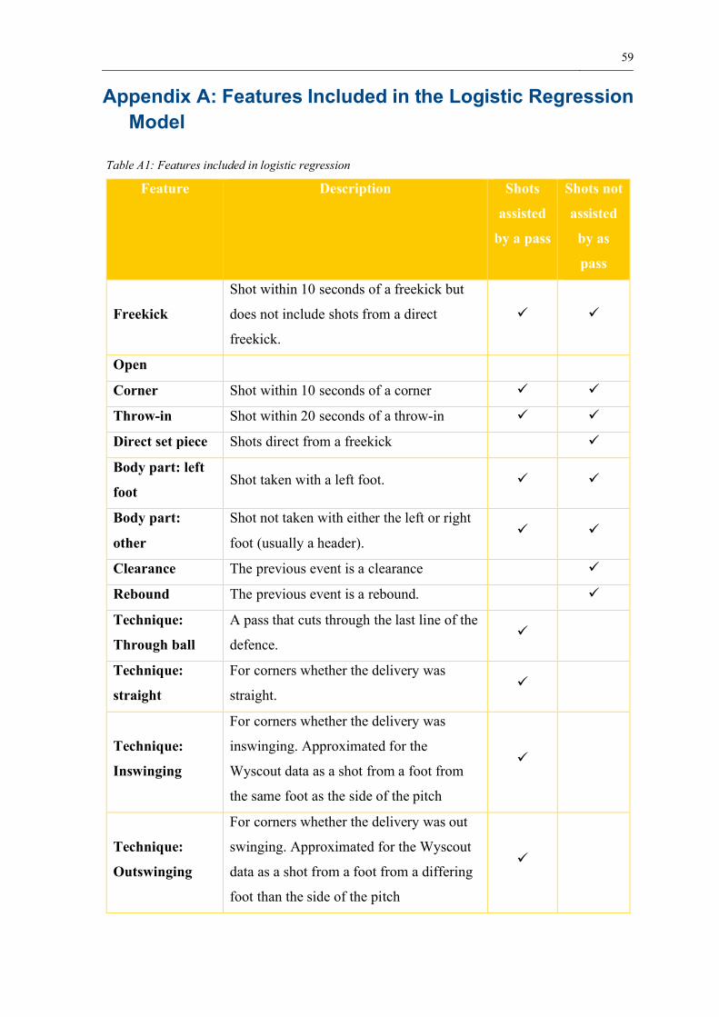
59

Appendix A: Features Included in the Logistic RegressionModel

Table A1: Features included in logistic regression

Feature Description Shots

assisted

by a pass

Shots not

assisted

by as

pass

Freekick

Shot within 10 seconds of a freekick but

does not include shots from a direct

freekick.

Open

Corner Shot within 10 seconds of a corner

Throw-in Shot within 20 seconds of a throw-in

Direct set piece Shots direct from a freekick

Body part: left

footShot taken with a left foot.

Body part:

other

Shot not taken with either the left or right

foot (usually a header).

Clearance The previous event is a clearance

Rebound The previous event is a rebound.

Technique:

Through ball

A pass that cuts through the last line of the

defence.

Technique:

straight

For corners whether the delivery was

straight.

Technique:

Inswinging

For corners whether the delivery was

inswinging. Approximated for the

Wyscout data as a shot from a foot from

the same foot as the side of the pitch

Technique:

Outswinging

For corners whether the delivery was out

swinging. Approximated for the Wyscout

data as a shot from a foot from a differing

foot than the side of the pitch

60

High passBall above the shoulder level (StatsBomb)

or 1 metre or higher (Wyscout)

Counterattack

Whether a shot was from a counterattack.

This comes from the counterattacking

logic from Wyscout4/ StatsBomb5

Fast break

Engineered feature: whether the team wins

the ball in own third and shoots in the last

quarter of the pitch within 25 seconds.

Strong foot

Engineered feature: whether the shot is

taken with the strongest foot (Wyscout) or

the foot used most often in events

(StatsBomb)

Switch

For pass assists whether the pass crossed

over 50% of the pitch vertically

(StatsBomb definition)

Cross StatsBomb definition 5

Cut-back StatsBomb definition 5

Visible angle Calculated as in Figure 3.

Middle angle Calculated as in Figure 3.

Distance to goal Calculated as in Figure 3.

Interaction

distance to the

goal and visible

angle

The distance to the goal multiplied by the

visible angle.

Log distance to

the goal

The natural logarithm of the distance to the

goal

4 Available at https://footballdata.wyscout.com/events-manual/5 Available at https://github.com/statsbomb/open-data/blob/master/doc/Open%20Data%20Events%20v4.0.0.pdf

61

Appendix B: Features Included in the Light GradientBoosting Machine Model

Table B1: Features included in the light gradient boosting machine model

Feature Description

xThe x coordinate of the shot taker from 0 to 105. Where 0 is the

shot takers goal line and 105 is the opponent’s goal line.

yThe y coordinate of the shot taker from 0 to 68. Where 0 is the

right touchline and 68 is the left touchline.

Goalkeeper x The goalkeeper x coordinate (same coordinate reference as x/y)

Goalkeeper y The goalkeeper y coordinate (same coordinate reference as x/y)

Pass end x The assisting pass x coordinate (same coordinate reference as x/y)

Pass end y The assisting pass y coordinate (same coordinate reference as x/y)

Carry LengthThe distance between where the end location of the assisting pass

and the location of the shot (only calculated for StatsBomb data)

Body part

name

Whether the shot was taken with the left foot, right foot, or another

body part (usually head)

N angle The number of players in the visible angle to the goal

Shot type

name

One of open play, free kick (if within 10 seconds of a free kick),

corner (if within 10 seconds of a corner) or throw-in (if within 20

seconds of an attacking throw-in. The closest event is taken for

set-pieces when there is more than one event in the timeframe.

Shot open goalWhether the shot was taken into an open goal (no defending

players)

Pass technique

name

The technique for crosses one of straight, inswinging, or out

swinging and whether the pass was a through ball (see Table A1

for definitions for each of these techniques).

Area goal

The area around the goalkeeper. Calculated as the area from a

Voronoi diagram, i.e. the area where the goalkeeper is the closest

player to that point on the pitch.

Area shot

The area around the shot taker. Calculated as the area from a

Voronoi diagram, i.e. the area where the shot taker is the closest

player to that point on the pitch.

62

Pass cross StatsBomb definition5

Pass cut-back StatsBomb definition5

Pass switch StatsBomb definition5

Strong footEngineered feature: whether the shot is taken with the strongest

foot (Wyscout) or the foot used most often in events (StatsBomb)

Assist typeThe assist type, which is one of pass, recovery, clearance, direct,

or rebound

CounterattackWhether a shot was from a counterattack. This comes from the

counterattacking logic from Wyscout4/ StatsBomb5

Pass heightHigh if the ball is above the shoulder level (StatsBomb) or 1 metre

or higher (Wyscout). Otherwise a single category ground/low.

Under

pressureWhether the shot was taken under pressure. StatsBomb definition5

Shot one on

oneWhether the shot was a 1 versus 1 situation.

Fast breakEngineered feature: whether the team wins the ball in own third

and shoots in the last quarter of the pitch within 25 seconds.

Smart pass Wyscout definition 4