FLUID MECHANICS FOR CIVIL ENGINEERING Chapter 4: Flow in Pipelines

SEQUENCE OF CHAPTER 4IntroductionObjectives4.1 Pipe Flow System4.2 Types of Flow

4.2.1 Laminar Flow4.2.2 Turbulent Flow

4.3 Energy Losses due to Friction4.3.1 Friction Losses in Laminar Flow4.3.2 Friction Loss in Turbulent Flow

4.4 Minor Losses4.4.1 Losses due to Pipe Fittings4.4.2 Sudden Enlargement4.4.3 Sudden Contraction

4.5 Energy Added and Extracted4.6 Pipe Flow Analysis

4.6.1 Simple Pipeline4.6.2 Pipes in Series4.6.3 Pipes in Parallel4.6.4 Pipe Network

Summary

Introduction

In considering the convenience and necessities in every day life, it is truly amazing to note the role played by conduits in transporting fluid.

For example, the water in our homes is normally conveyed through pressure pipelines, from the distribution system, so that it will be available when and where we want it.

Moreover, virtually all of this water leaves our homes as dilute wastes through sewers, another type of conduits. Oil is often transferred from their source by pressure pipelines to refineries while gas is conveyed by pipelines into a distribution network for supply.

Thus, it can be seen that the fluid flow in conduits is of immense practical significance in civil engineering.

Objectives

1. Differentiate between laminar and turbulent flows in pipelines.

2. Describe the velocity profile for laminar and turbulent flows.

3. Compute Reynolds number for flow in pipes.

4. Define the friction factor, and compute the friction losses in pipelines.

5. Recognize the source of minor losses, and compute minor losses in pipelines.

6. Analyze simple pipelines, pipelines in series, parallel, and simple pipe networks.

4.1 Pipe Flow System

• This chapter introduces the fundamental theories of flow in pipelines as well as basic design procedures.

• In this chapter, the pipeline system is defined as a closed conduit with a circular cross-section with water flows (flowing full) inside it.

• It is a closed system, the water is not in contact with air (i.e. no free surface). Flow in a closed pipe results from a pressure difference between inlet and outlet. The pressure is affected by fluid properties and flow rate.

• The following diagram gives the geometrical properties for circular pipe. In the diagram, D represents the diameter of pipe, R is the pipe radius and L is the pipe length. The cross-sectional area of the pipe can be calculated using A = R2.

In hydraulic applications, energy values are often converted into units of energy per unit weight of fluid, resulting in units of length.

When using these length equivalents, the energy of the system is expressed in terms of ‘head.’ The usual unit used is meter. The energy at any point within a hydraulic system is often expressed in three parts, i.e. the pressure head (P/g), elevation head (z), and velocity head (V2/2g) The sum of all these components is known as the total head (H).

(4.1)

RR

D=2R

L

R

PipeCenterline

Figure 4.2: Schematic diagram of a circular pipe

g2

Vz

g

PH

2

Figure 4.3: Flow in a uniform pipeline

A line plotted of total head versus distance through a system is called the total energy line (TEL).

The TEL is also known as energy grade line (EGL). The sum of the elevation head and pressure head yields the

hydraulic grade line (HGL). In a uniform pipeline, the total shear stress (resistance to flow) is

constant along the pipe resulting in a uniform degradation of the total energy or head along the pipeline.

The total head loss along a specified length of pipeline is referred to head loss due to friction and denoted as hf.

Referring to the above figure, the Bernoulli equation can be written from section 1 to section 2 as;

(4.2)f

22

22

21

11 h

g2

Vz

g

P

g2

Vz

g

P

4.2 Types of Flow• The physical nature of fluid flow can be categorized into three

types, i.e. laminar, transition and turbulent flow. It has been mentioned earlier that Reynolds Number (Re) can be used to characterize these flow.

(4.3)

where = density = dynamic viscosity = kinematic viscosity ( = /)V = mean velocity D = pipe diameter

In general, flow in commercial pipes have been found to conform to the

following condition:Laminar Flow: Re <2000Transitional Flow : 2000 < Re <4000Turbulent Flow : Re >4000

VDVD

Re

4.2.1 Laminar flow Viscous shears dominate in this type of flow and

the fluid appears to be moving in discreet layers. The shear stress is governed by Newton’s law of viscosity (equation 1.1):

(1.1)

In general the shear stress is almost impossible to measure. But for laminar flow it is possible to calculate the theoretical value for a given velocity, fluid and the appropriate geometrical shape.

dy

du

Pressure loss during a laminar flow in a pipe Up to this point we only considered ideal fluid

where there is no losses due to friction or any other factors.

In reality, because fluids are viscous, energy is lost by flowing fluids due to friction which must be taken into account.

The effect of friction shows itself as a pressure (or head) loss. In a pipe with a real fluid flowing, the shear stress at the wall retard the flow.

The shear stress will vary with velocity of flow and hence with Re. Many experiments have been done with various fluids measuring the pressure loss at various Reynolds numbers.

Figure below shows a typical velocity distribution in a pipe flow. It can be seen the velocity increases from zero at the wall to a maximum in the mainstream of the flow.

Figure 4.4: A typical velocity distribution in a pipe flow

In laminar flow the paths of individual particles of fluid do not cross, so the flow may be considered as a series of concentric cylinders sliding over each other – rather like the cylinders of a collapsible pocket telescope.

Lets consider a cylinder of fluid with a length L, radius r, flowing steadily in the center of pipe.

Figure 4.5: Cylindrical of fluid flowing steadily in a pipe

The fluid is in equilibrium, shearing forces equal the pressure forces.

Shearing force = Pressure force

(4.5)

Taking the direction of measurement r (measured from the center of pipe), rather than the use of y (measured from the pipe wall), the above equation can be written as;

(4.6)

Equating (4.5) with (6.6) will give:

2

r

L

P

rPPArL2 2

dr

du r

2

r

L

P

dr

dudr

du

2

r

L

P

In an integral form this gives an expression for velocity, with the values of r = 0 (at the pipe center) to r = R (at the pipe wall)

(4.7)

where P = change in pressure L = length of pipe

R = pipe radius r = distance measured from the center of pipe

The maximum velocity is at the center of the pipe, i.e. when r = 0.

It can be shown that the mean velocity is half the maximum velocity, i.e. V=umax/2

Rr0r rdr

2

1

L

Pu

L

P

4

rRu

22

r

L

P

4

Ru

2

max

Figure 6.6: Shear stress and velocity distribution in pipe for laminar flow

The discharge may be found using the Hagen-Poiseuille equation, which is given by the following;

(4.8)

The Hagen-Poiseuille expresses the discharge Q in terms of the pressure gradient , diameter of pipe, and viscosity of the fluid.

Pressure drop throughout the length of pipe can then be calculated by (4.9)

128

D

L

PQ

4

L

P

dx

dP

4R

LQ8P

4.2.2 Turbulent flow This is the most commonly occurring flow in engineering

practice in which fluid particles move erratically causing instantaneous fluctuations in the velocity components.

These fluctuations cause additional shear stresses. In this type of flow both viscous and turbulent shear stresses exists.

Thus, the shear stress in turbulent flow is a combination of laminar and turbulent shear stresses, and can be written as:

where = dynamic viscosity = eddy viscosity which is not a fluid property but

depends upon turbulence condition of flow.

dy

dUturbulentarminla

The velocity at any point in the cross-section will be proportional to the one-seventh power of the distance from the wall, which can be expressed as:

(4.10)

where Uy is the velocity at a distance y from the wall, UCL is the velocity at the centerline of pipe, and R is the radius of pipe. This equation is known as the Prandtl one-seventh law.

Figure 6.7 below shows the velocity profile for turbulent flow in a pipe. The shape of the profile is said to be logarithmic.

7/1

CL

y

R

y

U

U

Figure 4.7: Velocity profile for turbulent flow

For smooth pipe:

(4.11a)

For rough pipe:

(4.11b)

In the above equations, U represents the velocity at a distance y

from the pipe wall, U* is the shear velocity =

y is the distance form the pipe wall, k is the surface roughness and

is the kinematic viscosity of the fluid.

5.5yU

log75.5U

U *10

*

5.8k

ylog75.5

U

U10

*

Example 4.1

Glycerin ( = 1258 kg/m3, =9.60 x10-1 N.s/m2) flows with a velocity of 3.6 m/s in a 150-mm diameter pipe. Determine whether the flow is laminar or turbulent.

Solution:

Since Re=708, which is less than 2000, the flow is laminar.

VD

Re

70810x60.9

15.0x6.3x1258Re

1

4.3 Energy Losses due to friction

When a liquid flows through a pipeline, shear stresses develop between the liquid and the pipe wall.

This shear stress is a result of friction, and its magnitude is dependent upon the properties of the fluid, the speed at which it is moving, the internal roughness of the pipe, the length and diameter of pipe.

Friction loss, also known as major loss, is a primary cause of energy loss in a pipeline system.

4.3.1 Friction Losses in Laminar flow In laminar flow, the fluid seems to flow as several layers, one on

another. Because of the viscosity of the fluid, a shear stress is created between the layers of fluid.

Energy is lost from the fluid to overcome the frictional forces produced by the shear stress.

Energy loss is usually represented by the drop of pressure in the direction of flow.

Therefore, the frictional head loss, hf, can be written in terms of pressure drop along the pipeline, as follows:

(4.12)

Substituting the Hagen-Poiseuille equation and applying the continuity equation, Q = VA, to the above resulted into the following expression:

(4.13)

g

Ph f

g2

V

D

L

Re

64

gD

LV32h

2

2f

4.3.2 Friction Losses in Turbulent flow In turbulent flow, the friction head loss can be calculated by

considering the pressure losses along the pipelines.

In a horizontal pipe of diameter D carrying a steady flow there will be a pressure drop in a length L of the pipe.

Equating the frictional resistance to the difference in pressure forces, and manipulating resulted into the following expression:

(4.14)

This equation is known as Darcy-Weisbach (D-W) equation, in which is the friction factor. It should be noted that is dimensionless, and the value is not constant

g2

V

D

Lh

2

f

Blasius (1913) was the first to propose an accurate empirical relation for the friction factor in turbulent flow in smooth pipes, namely

(4.15)

Thus, the calculation of losses in turbulent pipe flow is dependent on the use of empirical results and the most common reference source is the Moody diagram. A Moody diagram is a logarithmic plot of vs. Re for a range of k/D. A typical Moody diagram is shown in Figure 4.9.

= 0.316/Re0.25

Figure 4.8: Moody Diagram

Table 4.1: Typical pipe roughness

(Reference: White, 1999)Material Roughness, k (mm)

Glass smooth

Brass, new 0.002

ConcreteSmoothedRough

0.042.0

IronCast, newGalvanised, newWrought, new

0.260.150.046

SteelCommercial, newRiveted

0.0463

4.4 Minor Losses

• In addition to head loss due to friction, there are always other head losses due to pipe expansions and contractions, bends, valves, and other pipe fittings. These losses are usually known as minor losses (hLm).

• In case of a long pipeline, the minor losses maybe negligible compared to the friction losses, however, in the case of short pipelines, their contribution may be significant.

6.4.1 Losses due to pipe fittings

where hLm= minor loss

K = minor loss coefficient V = mean flow velocity

g2

VKh

2

Lm (6.16)

Table 4.2: Typical K values

Type K

Exit (pipe to tank) 1.0

Entrance (tank to pipe)

0.5

90 elbow 0.9

45 elbow 0.4

T-junction 1.8

Gate valve 0.25 - 25

4.4.2 Sudden Enlargement As fluid flows from a smaller pipe into a larger pipe through

sudden enlargement, its velocity abruptly decreases; causing turbulence that generates an energy loss.

The amount of turbulence, and therefore the amount of energy, is dependent on the ratio of the sizes of the two pipes.

The minor loss (hLm)is calculated from;

(4.16a)

where is KE is the coefficient of expansion, and the values depends on the ratio of the pipe diameters (Da/Db) as shown below.

g2

VKh

2a

ELm

Da/Db 0.0 0.2 0.4 0.6 0.8

K 1.00 0.87 0.70 0.41 0.15

Table 4.3: Values of KE vs. Da/Db

Figure 4.9: Flow at Sudden

Enlargement

4.4.3 Sudden ContractionThe energy loss due to a sudden contraction can be calculated using the following;

(4.16b)

The KC is the coefficient of contraction and the values depends on the ratio of the pipe diameter (Db/Da) as shown below.

g2

VKh

2b

CLm

Db/Da 0.0 0.2 0.4 0.6 0.8 1.0

K 0.5 0.49 0.42 0.27 0.20 0.0

Table 4.4: Values of KC vs. Db/Da

Figure 4.10: Flow at sudden contraction

Example 4.2 Water at 10C is flowing at a rate of 0.03 m3/s through a pipe. The

pipe has 150-mm diameter, 500 m long, and the surface roughness is estimated at 0.06 mm. Find the head loss and the pressure drop throughout the length of the pipe.

Solution: From Table 1.3 (for water): = 1000 kg/m3 and =1.30x10-3 N.s/m2

V = Q/A and A=R2

A = (0.15/2)2 = 0.01767 m2

V = Q/A =0.03/.0.01767 =1.7 m/sRe = (1000x1.7x0.15)/(1.30x10-3) = 1.96x105 > 2000 turbulent

flowTo find , use Moody Diagram with Re and relative roughness (k/D).

k/D = 0.06x10-3/0.15 = 4x10-4

From Moody diagram, 0.018The head loss may be computed using the Darcy-Weisbach equation.

The pressure drop along the pipe can be calculated using the relationship: ΔP=ghf = 1000 x 9.81 x 8.84ΔP = 8.67 x 104 Pa

.m84.881.9x2x15.0

7.1x500x018.0

g2

V

D

Lh

22

f

Example 4.3 Determine the energy loss that will occur as 0.06 m3/s water

flows from a 40-mm pipe diameter into a 100-mm pipe diameter through a sudden expansion.

Solution: The head loss through a sudden enlargement is given by;

Da/Db = 40/100 = 0.4From Table 6.3: K = 0.70Thus, the head loss is

g2

VKh

2a

m

s/m58.3)2/04.0(

0045.0

A

QV

2a

a

m47.081.9x2

58.3x70.0h

2

Lm

4.5 Energy added and extracted

• There are many occasions when energy needs to be added to a hydraulic system to overcome elevation differences, friction losses and minor losses.

• A pump is a common device to which mechanical energy is applied and transferred to the water as total head of the pump.

• The head added is called pump head (Hp), and is a function of flow rate through the pump.

• On the other hand, fluid motor or turbines are common examples of devices that extract energy from a fluid, and the head extracted is called head of turbine (Ht), deliver it in a form of work.

Denoting the head loss due to friction and minor losses as HL, and the external energy added/extracted by HE, then the Bernoulli equation may be rewritten as

(4.17)

HE = Hp (positive for pump) when the head is added to the fluid, or HE = Ht (negative for turbine) when the head is extracted from the fluid. Note the similarity of this equation with equation (3.12). It is often necessary to convert the total power (P) of a pump or turbine to HE or vice versa. Recall from Chapter 3, the relationship between P and HE is given by the following

P = gQHE (3.8)

In a pump HE = HP, the value is positive since power is added to the fluid. In a turbine, HE = Ht is negative and power is extracted from the flow.

21L

22

22

E

21

11 H

g2

Vz

g

PH

g2

Vz

g

P

The term efficiency is used to denote the ratio of the power delivered by the pump to the fluid to the power supplied to the pump.

Because of energy loses due to mechanical friction in pump components, fluid friction in the pump, and excessive fluid turbulence in the pump, not all of the input power is delivered to the fluid. Therefore, the efficiency of a pump can be written as;

The value of p is less than 1.0. Similarly, energy losses in a turbine are produced by mechanical

and fluid friction. Therefore, not all the power delivered to the motor is ultimately converted to power output from the device. The efficiency of a turbine is defined as;

Here again, the value of t is less than 1.0.

in

p

inp P

gQH

P

P

pumptopliedsupPower

fluidtodeliveredPower

t

o

t

ot gQH

P

P

P

fluidbypliedsupPower

motorfromoutputPower

Example 4.4

Calculate the head added by the pump when the water system shown below carries a discharge of 0.27 m3/s. If the efficiency of the pump is 80%, calculate the power input required by the pump to maintain the flow.

Solution:Applying Bernoulli equation between section 1 and 2

(1)

P1 = P2 = Patm = 0 (atm) and V1=V2 0 Thus equation (1) reduces to:

(2)

HL1-2 = hf + hentrance + hbend + hexit

From (2):

21L

22

22

p

21

11 H

g2

Vz

g

PH

g2

Vz

g

P

21L12p HzzH

g2

V4.39

14.05.04.0

1000x015.0

g2

VH

2

2

21L

81.9x2

V4.39200230H

2

p

The velocity can be calculated using the continuity equation:

Thus, the head added by the pump: Hp = 39.3 m

Pin = 130 117 Watt ≈ 130 kW.

s/m15.2

2/4.0

27.0

A

QV

2

in

pp P

gQH

8.0

3.39x27.0x81.9x1000gQHP

p

pin

4.6 Pipe Flow Analysis

• Pipeline system used in water distribution, industrial application and in many engineering systems may range from simple arrangement to extremely complex one.

• Problems regarding pipelines are usually tackled by the use of continuity and energy equations.

• The head loss due to friction is usually calculated using the D-W equation while the minor losses are computed using equations 4.16, 4.16(a) and 4.16(b) depending on the appropriate conditions.

4.6.2 Pipes in Series

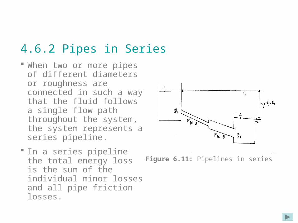
When two or more pipes of different diameters or roughness are connected in such a way that the fluid follows a single flow path throughout the system, the system represents a series pipeline.

In a series pipeline the total energy loss is the sum of the individual minor losses and all pipe friction losses.

Figure 6.11: Pipelines in series

Referring to Figure 4.11, the Bernoulli equation can be written between points 1 and 2 as follows;

(4.18)where P/g = pressure head

z = elevation headV2/2g = velocity headHL1-2 = total energy lost between point 1 and 2

Realizing that P1=P2=Patm, and V1=V2, then equation (4.14) reduces to

z1-z2 = HL1-2

Or we can say that the different of reservoir water level is equivalent to the total head losses in the system.

The total head losses are a combination of the all the friction losses and the sum of the individual minor losses.

HL1-2 = hfa + hfb + hentrance + hvalve + hexpansion + hexit.

Since the same discharge passes through all the pipes, the continuity equation can be written as; Q1 = Q2

21L

22

22

21

11 H

g2

Vz

g

P

g2

Vz

g

P

4.6.3 Pipes in Parallel• A combination of two

or more pipes connected between two points so that the discharge divides at the first junction and rejoins at the next is known as pipes in parallel. Here the head loss between the two junctions is the same for all pipes.

Figure 4.12: Pipelines in parallel

Applying the continuity equation to the system;

Q1 = Qa + Qb = Q2 (4.19)

The energy equation between point 1 and 2 can be written as;

The head losses throughout the system are given by;

HL1-2=hLa = hLb (4.20)

Equations (4.19) and (4.20) are the governing relationships for parallel pipe line systems. The system automatically adjusts the flow in each branch until the total system flow satisfies these equations.

L

22

22

21

11 H

g2

Vz

g

P

g2

Vz

g

P

4.6.4 Pipe Network

A water distribution system consists of complex interconnected pipes, service reservoirs and/or pumps, which deliver water from the treatment plant to the consumer.

Water demand is highly variable, whereas supply is normally constant. Thus, the distribution system must include storage elements, and must be capable of flexible operation.

Pipe network analysis involves the determination of the pipe flow rates and pressure heads at the outflows points of the network. The flow rate and pressure heads must satisfy the continuity and energy equations.

The earliest systematic method of network analysis (Hardy-Cross Method) is known as the head balance or closed loop method. This method is applicable to system in which pipes form closed loops. The outflows from the system are generally assumed to occur at the nodes junction.

For a given pipe system with known outflows, the Hardy-Cross method is an iterative procedure based on initially iterated flows in the pipes. At each junction these flows must satisfy the continuity criterion, i.e. the algebraic sum of the flow rates in the pipe meeting at a junction, together with any external flows is zero.

• Assigning clockwise flows and their associated head losses are positive, the procedure is as follows: Assume values of Q to satisfy Q = 0. Calculate HL from Q using HL = K1Q2 . If HL = 0, then the solution is correct. If HL 0, then apply a correction factor, Q, to all Q and repeat

from step (2). For practical purposes, the calculation is usually terminated

when HL < 0.01 m or Q < 1 L/s. A reasonably efficient value of Q for rapid convergence is given

by;

(4.21)

QH2

HQ

L

L

Example 4.5• A pipe 6-cm in diameter, 1000m long and with =

0.018 is connected in parallel between two points M and N with another pipe 8-cm in diameter, 800-m long and having = 0.020. A total discharge of 20 L/s enters the parallel pipe through division at A and rejoins at B. Estimate the discharge in each of the pipe.

Solution:Continuity: Q = Q1 + Q2

(1)

Pipes in parallel: hf1 = hf2

Substitute (2) into (1)

0.8165V2 + 1.778 V2 = 7.074

V2 = 2.73 m/s

22

221

2 V)08.0(4

V)06.0(4

02.0

074.7V778.1V 21

)2(V8165.0V

V08.0

800x020.0V

06.0

1000x018.0

gD2

VL

gD2

VL

21

22

21

2

222

21

211

1

Q2 = 0.0137 m3/s

From (2):V1 = 0.8165 V2 = 0.8165x2.73 = 2.23 m/s

Q1 = 0.0063 m3/s

Recheck the answer:Q1+ Q2 = Q0.0063 + 0.0137 = 0.020 (same as given Q OK!)

73.2x)08.0(4

VAQ 2222

Example 4.6 • For the square loop shown, find the discharge in all

the pipes. All pipes are 1 km long and 300 mm in diameter, with a friction factor of 0.0163. Assume that minor losses can be neglected.

Solution: Assume values of Q to satisfy continuity equations all at

nodes.

The head loss is calculated using; HL = K1Q2

HL = hf + hLm

But minor losses can be neglected: hLm = 0

Thus HL = hf

Head loss can be calculated using the Darcy-Weisbach equation g2

V

D

Lh

2

f

First trial

Since HL > 0.01 m, then correction has to be applied.

554'

'

554

3.04

77.277.2

81.923.0

10000163.0

2

2

2

22

2

2

2

2

2

K

QKH

QH

x

Qx

A

QH

x

VxxH

g

V

D

LhH

L

L

L

L

fL

Pipe Q (L/s) HL (m) HL/Q

AB 60 2.0 0.033

BC 40 0.886 0.0222

CD 0 0 0

AD -40 -0.886 0.0222

2.00 0.0774

Second trial

Since HL ≈ 0.01 m, then it is OK.Thus, the discharge in each pipe is as follows (to the nearest integer).

s/L92.120774.0x2

2

QH2

HQ

L

L

Pipe Q (L/s) HL (m) HL/Q

AB 47.08 1.23 0.0261

BC 27.08 0.407 0.015

CD -12.92 -0.092 0.007

AD -52.92 -1.555 0.0294

-0.0107 0.07775

Pipe Discharge (L/s)

AB 47

BC 27

CD -13

AD -53

Summary

Overall, chapter 4 has introduced basic design procedures of a flow in pipelines and more elaboration on the type of flows.

A detail calculation of pipe flow analysis which consists of simple pipeline, pipe in series, pipe in parallel and pipe network were discussed.

The pipe network used the Hardy Cross method and at the end, the discharge of water of each pipe can be known.