1

Financial crisis and Tobin Taxation: an event analysis

Theodoros Bratis Department of Business Administration, Athens University of Economics and Business, 76

Patission Street, Athens 10434, Greece, Email: tbratis@aueb.gr

Nikiforos T. Laopodis

ALBA Graduate Business School at the American College of Greece 6-8 Xenias Street, Athens 11527, Greece, email: nlaopodi@alba.edu.gr

Georgios P. Kouretas* IPAG Business School,

184 Boulevard Saint-Germain, FR-75006, Paris, France and

Department of Business Administration, Athens University of Economics and Business, 76 Patission Street, Athens 10434, Greece, email: kouretas@aueb.gr (corresponding author)

7 March 2016

Abstract

Under the context of EMU debt and financial crisis we assess the impact of EMU’s

legislative initiative on Tobin tax for financial regulation. Specifically we focus on its

impact on bond and equity volatility for a representative basket of 7 countries:

Germany, France (core EMU) and Greece, Italy, Ireland, Portugal and Spain

(periphery EMU). In the absence of historical data on volume and volatility of

transactions of a (simultaneous) security transaction tax (STT), we derive a pure event

analysis. Secondly we expect the announcement of the tax decision to impact

volatility in bond/equity market. We find evidence for the core and periphery EMU

bond return portfolio (under both approaches) and core equity EMU under the event

study methodology.

Keywords: Tobin tax, financial crisis, regulation, event study, GARCH

JEL classification: G01, G15, F34. * An earlier version was presented at the 13th INFINITI Conference on International Finance, Ljubljana 8-9 June 2015. The paper has benefited from helpful comments and discussions by seminar participants at Athens University of Economics and Business and University of Piraeus. Kouretas acknowledges financial support from a Marie Curie Transfer of Knowledge Fellowship of the European Community's Sixth Framework Programme under contract number MTKD-CT-014288, as well as from the Research Committee of the University of Crete under research grant #2257. We thank Jonathan Batten, Stelios Bekiros, Sris Chatterjee, Alex Cukierman, Manthos Delis, Bill Francis, Dimitris Georgoutsos, Iftekhar Hasan, Alexandros Kontonikas and the discussant Georgios Georgiadis for many helpful comments and discussions. The usual caveat applies. 1 Department of Business Administration, Athens University of Economics and Business, 76 Patission Street , GR110434, Athens, Greece. Email address: tbratis@aueb.gr 2 ALBA Graduate School at the American College of Greece Email address: nlaopodi@alba.edu.g 3 IPAG Business School, 184 Boulevard Saint-Germain, FR-75006, Paris, France. * Corresponding author : Tel: 00302108203277, 00302108226203, fax: 00302108226203. Email address: kouretas@aueb.gr.

2

1. Introduction

The financial crisis of 2007-2009 and the subsequent Eurozone debt crisis

exposed flaws in the global financial architecture and International Monetary System

(IMS). The former argument and the ongoing financial instability brought in the

surface the need of restructuring the regulation framework of the global financial

markets (in terms of a macro prudential regulation), due to the fiscal and monetary

cost governments face and to the fact that no country has financial immunity.

According to Alworth and Arachi (2010): “the financial sector is prone to two types

of problems requiring correction (i) distorted incentive structures and undesired

behavior of economic agents (moral hazard) and/or (ii) externalities within the

financial sector (the failure of an institution propagating amongst one another) and

from the financial sector to the real economy (systemic risk)”.

Markets’ inabilities to self-regulate by sustaining imperfections-and thus

disequilibrium in financial markets pose a severe externality to global growth through

the systemic risk. The latter is propagated mainly through systemically important

financial institutions i.e. the disturbance of lending channel (by intensifying the

problem of moral hazard) and thus of investment in aggregate demand, hence

according to theory the most prominent tactic is taxing the source of externality.

Furthermore as Brunnermeier et al. (2009) state: “Externalities are by far the most

important reason why banks, and other key financial intermediaries and markets, need

regulation”. According to Claessens et al. (2010) macro-prudential externalities relate

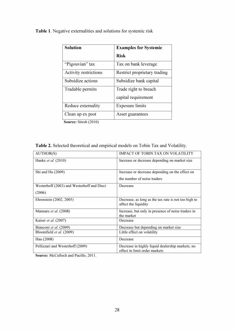
to systemic risk1. Stiroh (2010) discusses the main externalities of financial markets

and provides the possible solution in terms of public finance given in Table 1.

1 “The failure or distress of one institution can have domino effects on other institutions or clients. Brunnermeier et al. (2009) argues that the key channels of transmission are: direct financial exposures, market exposures, or reputational exposures. Additionally, externalities may arise in forms of

3

Market failures can be remedied by targeted fiscal policy as the Keynesian

School of thought argues. In general, capital control is based on administrative or tax

measures. Tax policy reduces the financial system’s entropy by the realignment of

participating agents’ incentives towards the expected desired outcome. As

Masciandaro and Passarelli (2013) argue: “in a perfect Pigouvian world, taxation and

regulation would be equivalent: both policies can achieve a first best outcome if well

calibrated to deal with systemic risk (externality resulting from contagion effects), but

in the real world financial regulation is largely preferred”. On the other hand it is also

debatable whether only tax measures halt crisis episodes without additional regulatory

framework and monitoring. Furthermore the increased cost of financial transactions

caused by such a policy threatens markets’ equilibrium by influencing arbitrage

perception.

Policy makers dealing the ongoing crisis presented a grid of solutions. IMF

responding to G20 call (September 2009) for policy options on the contribution of

banking sector in the burdens associated with government interventions and the repair

of the banking system, adopted two measures; levies in financial institutions (in terms

of raising funds for future crises) and generally increased revenues from sectors’

activities through financial transaction taxes (FTTs) or as favoured through financial

activities taxes (FATs) (Claessens et al., 2010, p. 144)2. Moreover, as Matheson

(2012) argues: “financial transaction taxes particularly securities transaction taxes

(STTs) and/ or currency transaction taxes (CTTs or Tobin taxes) have come under

widespread serenity as a result of the recent financial crisis as well as general global

economic developments”.

‘excessive’ volatility of asset prices, including exchange rates, and related excessive volatility of financial and capital flows” (p. 48) 2 According to Shaviro (2012) FAT focuses on a broad “net” measure, rather than a narrow “gross” of financial activity sector like FTT but as measures are commonly viewed as exclusive alternatives.

4

In light of the previous arguments the European Commission in its budget

proposal for 2014-2020 has included the introduction of a Tobin tax type in financial

transactions (FTT), that is directed mainly at secondary securities trading (Shaviro,

2012), as a means of (1) raising revenue, (2) ensuring an “adequate (fair and

substantial)” contribution from the financial sector, (3) “reducing undesirable market

behavior and thereby stabilizing markets,” and (4) achieving coordination between

different Member States’ internal taxes (European Commission 2011a, p. 3-4). 3

Particularly the tax proposal will apply to shares and bonds and derivatives on

shares and bonds. The ad valorem tax is about (member states are free to charge

higher rates) 0.1% on the first category and 0.01% on the second one (over

derivatives’ nominal value of the underlying asset) over financial transactions carried

out by Financial Institutions (except Central Banks) in organized and over the counter

markets (only secondary markets), according to the residence principle (i.e. at least

one of the taxed parties entering transaction is situated in the EU or the security is

issued by a firm in a taxed jurisdiction).

It is expected that primary markets will be indirectly affected by the increased

cost on the secondary markets. Different tax rates between similar financial

instruments may cause a shift in demand towards substitute speculative products.

Under this consideration there exists the danger for transitory excess volatility and

thus greater risk for the potential investors. Moreover, any implemented policy

should be balanced because of the asymmetric information challenges posed. Excess

taxation will result to specific investment aversion (adverse selection); withdraw of

interest and capital and thus leading long term to asset market crushes and

3 http://ec.europa.eu/budget/biblio/documents/fin_fwk1420/fin_fwk1420_en.cfm

5

overinvestment and liquidity bubbles (increased volatility) in secondary connected

markets.

The outcome (on collecting public revenue through the implementation of the

tax) suggests that a reduction in national percentage participation in EU budgeting is

capable. Secondly, the outcome makes even more feasible the correction of financial

markets’ disequilibrium (thus confronting volatility and asset price bubbles and

discourages risky behaviors). The amount to be collected is targeted to approximately

50 billion € per year or 350 billion € during the period of implementation with the EU

budget stable at 1.000 billion €. The two most known paradigms in Europe is that of

Sweden (1984-1990) and UK (Stamp Duty). The first paradigm is closer to the

ongoing EU’s proposal while the latter has emerged as a solution due to the

difficulties for a unanimous decision about the former. Moreover from August 1st

2012 the French Government enacted a FTT4 based on the type of securities traded.

EU initiative about imposing a Tobin type tax by exempting its application

over currency trade revert it to a plain security transaction tax (STT). It is certain that

the goal of the policy rests in raising revenue helping compensating for numerous

costs caused by the recent financial crisis besides reducing market risk (volatility) in

order to prevent asset price bubbles as already mentioned. Theoretically the

implementation of a security tax will raise the transaction cost of the traded

instrument and reduce its (short time) speculative trading volume. Also there is the

issue that a reduction of transactions (due to the tax wedge) may indeed lower

expected revenue collection thus the effectiveness of the proposal.

Generally the on-going banking and debt crisis in Europe has provided the

political chance for a theory implementation try-out in the following years to come

4 French model: 0,1% on listed French equities, 0,01% for high frequency trading and 0,01% for CDS on government bonds. The equities have a market cap of over 1 billion euro on the 1st of January of the year of taxation.

6

(2016-) on the basis of a common EU-115 Financial or Security Transaction Tax

(FTT/STT) on financial instruments for the secondary market. Thus the impact on

EU-11 (FTT Zone) presents a significant challenge given the previous applied studies

on the phenomenon.

To our knowledge there is a gap in the literature in implementing the

methodology of event study in any empirical finance literature for Tobin taxation.

Therefore besides the lack of historical data emphasizing the need for alternative

procedures (in measuring the impact of Tobin taxation) we contribute to the literature

by evaluating the taxation announcements effects under a new prism. In other words

we assess the financial regulation impact following markets’ reactions to the

unexpected event of the agreement on implementing a common European tax in

transactions. Secondly we assess whether the announcement affected the volatility of

equity/bond markets at the European level. Moreover we offer a cumulative literature

survey research on the topic.

The rest of the paper is organized as follows. Section 2 provides the literature

review. Section 3 presents and discusses the methodology used. Section 4 presents the

data and preliminary empirical results whereas Section 5 provides the main empirical

results. Section 6 provides our summary and concluding remarks.

2. Literature review

Tobin taxation has been named after James Tobin (1978) who proposed it

given the increased exchange rate volatility observed after the collapse of fixed

exchange rate system (Buiter, 2003). Nevertheless Tobin tax, besides the initial idea

on preventing speculative movements in trading currencies evolved as a generalized

idea on Financial Trade Transactions (FTT) i.e. on equities, bonds derivatives etc.

5 Austria, Belgium, Estonia, France, Germany, Greece, Italy, Portugal, Slovakia, Slovenia, Spain.

7

also including over-the-counter markets (Stiglitz, 1989; Summers and Summers,

1989; Schulmeister, Schratzenstaller and Picek, 2008). Caldari and Masini (2010)

have categorized the evolution on Tobin tax in three time spans: 1978-1994, 1994-

1998, 1998-present.6

Prior to Tobin other scholars such as Keynes (1936)-who was the first to

initiate the basic idea- and later Friedman (1953) engaged in the dialogue forming the

two conflicting pillars on applying taxation policy. Further studies7 continue the

controversial issue while some emphasize the significance of the dimension scale i.e.

globally or regionally, with respect to international cooperation in the context of cross

border financial institutions. Nevertheless, the Tobin Tax has had severe modern

critique8. Taxation in any form does not lead to optimal welfare utility and in parallel

distorts market participants’ incentives. Furthermore the application of a Tobin tax

shall reduce the trading of the financial instrument it will be based upon and thus its

price while the net reduction on volatility is likely to be small (Jürgen, 2012). But, this

tax also drives away investors who provide liquidity, stabilize prices, and help in the

price discovery process (Uppal, 2011).

Nevertheless it should be highlighted that the original idea of Tobin had global

perspective, instead of the applications by far that have different type variety in

different countries and different financial systems. A global Tobin transaction type tax

6 During the first it was ignored due to the prevail of liberal and neoliberal ideology, during the second it came to notice due to the emergence of the first severe global crises since the Great Depression of 1929 (the European Monetary System (1992-93); Mexico (1994); East Asian Countries (1997); Russia (1998); Brazil (1998-99); Argentina (1999-2000)) and during the third became the totem of financial anti-conformists. 7 According to Jürgen et al. (2012) “proponents claim that excessive trading facilitates long-term deviations of prices from fundamentals (‘bubbles’) as well as short-term deviations from fundamentals (‘excessive volatility’). Bubbles are costly because they lead to a misallocation of capital and increase the probability of a financial crisis as they collapse at some point in time. Excess volatility is costly to society, because it raises firms’ cost of investment and increases the probability of a financial crisis”. 8 Caldari and Masini (2010) emphasize the fact that the “UN World Economic and Social Survey 1995 dismissed Tobin Tax as “a sort of Luddite proposal”, in the sense that it was an anti-historical attempt to contrast the increasing liberalization of markets (p. 12). Moreover Caldari and Massini (2010) highlighted the reaction by Tobin himself on embracing the possibility of adopting taxes by a set of core countries instead of the difficulties in accepting its enactment on universal climax (p. 12).

8

assures that all market participants’ incentives are aligned. That is the idea behind

opposing to the adoption of that tax for a single country or union of countries (like

EU) unilaterally with the subsequent danger of tax avoidance and capital hemorrhage

and its migration to other financial centers. In that case it is doubtful if the expected

revenues will outperform the cost of mitigating systemic risk having in mind the

stabilization utility of the tax. Thus the feasibility and effectiveness of the tax is rather

questionable in the absence of a global pact.

Additionally a financial transaction tax behaves as a capital income tax by

lowering savings leading to current consumption enlargement (by raising the relative

cost of future consumption) or to current consumption decrease (due to reduced

wealth). However, unlike a capital income tax it taxes gross instead net flows

producing cascading or multiple taxation of the same product (allocation of assets and

risk across investors). Thus, “it is not possible to design a financial transaction tax that

imposes the same tax burden on all sets of financial transactions that deliver the same

economic outcome, leading to multiple taxation”, (Matheson 2012, p. 902).

Overall, the literature review reveals that any enactment of a Tobin type tax

will be ambiguous and have diversified results. There are two main categories; the

first including theoretical models of the Tobin type tax and the second one of

empirical models presenting evidence on the effects of its enactment. Particularly

theoretical models include Heterogeneous Agent Models9, “Zero Intelligence” (ZI)

models, game theory approaches and finally laboratory experiments or simulated

marketplaces for testing the previous. The second category has two main directions

regarding a) price: literature linking transaction costs and volatility (indirect approach

on Tobin type taxes effects) and fewer studies linking actual transaction taxes and

9 HAM models help to solve the “exchange rate determination puzzle” i.e. the disconnection of the exchange rate from its underlying fundamentals (Damette, 2013).

9

volatility. The majority of the empirical studies is over equity market and secondly on

currency market. There are also the additional branches concerning FTT impact on a)

liquidity and b) volume (see also Pomeranets, 2013 and McCulloch and Pacillo,

2011).

According to Uppal (2011) theoretical models due to different assumptions

give different conclusions and the majority of empirical studies [Ross (1989), Saporta

and Kan (1997), Umlauf (1993), Bessebinder and Rath (2002), Hau (2006), Aliber et

al. (2003)] find that a transaction tax either fails to reduce return volatility, or leads to

an increase in volatility. Furthermore, according to Uppal (2011) the theoretical

models under the enactment of a Tobin type tax are to be considered on the basis of

irrational traders with respect to the fundamental distinction among speculators and

non-speculators10

. McCulloch and Pacillo (2011) present their evidence on theoretical

and empirical models on Tobin Tax and Volatility given in Table 2.

Furthermore given that a Tobin tax has not yet been implemented (but only

taxes presenting a similarity to it), the authors use in their study as proxy the literature

linking transaction costs and volatility (p. 14-18). According to McCulloch and

Pacillo (2011), the literature also has some estimates of the elasticity of the volume of

trade in the foreign exchange market with respect to transaction costs (p. 36).

According to Jürgen et al. (2012) studies on directly assessing the

macroeconomic cost of a FTT do not exist. Matheson (2012) argues that there are two

types of volatility affected by the enactment of a financial transaction tax or a

currency transaction tax, short-term price volatility and long-term “boom and bust”

market cycles (p. 899). Furthermore Baldwin (2011) argues there are two volatility

10 Moreover, as Uppal (2011) argues: “The trading in financial markets by such investors generates volatility that is in excess to the volatility generated by macroeconomic fundamentals. The objective of the Tobin tax is to reduce the impact of these traders on financial markets, and hence, curb excess volatility”.

10

categories in literature: “Studies based on tick size (individual transactions) effects

treat volatility as the standard deviation of the mid-price return, not allowing for

robust cross-tick size regime volatility comparisons” and the modern opinion

presented as “a longer-term excesses of speculative prices”. Lavicka et al. (2013)

argue that according to literature the volatility of most financial instruments can be

decomposed into two parts a regular Gaussian component and a price jump

component. Thus generally the definition of volatility is disputed (as presented also in

McCulloch et al. (2011), p.17).

Our research is limited to compare results directly measuring the efficiency of

the tax concerning its connection to market volatility as Liau et al. (2012) did with AC

GARCH models. Liau et al. (2012) emphasizes the literature strand on linking asset

volatility and STTs following Aliber et al. (2003), Baltagi et al. (2006), Sanger et al.

(1990). We draw intuition from empirical studies concerning the impact of FTT on

price volatility: Roll (1989); Cambell and Froot (1994); Baltagi et al. (2006); Plylaktis

and Aristidou (2007); Chou and Wang 2006); Umlauf (1993); Hau (2006). In the

present study we expand empirical GARCH models by controlling for the tax

volatility effect in the conditional variance equation. Finally we follow McKinlay

(1997) in our event study approach.

The European Commission has been using dynamic stochastic general

equilibrium (DSGE) models for assessment of the macroeconomic impact of a Tobin

tax or of a security transaction tax (see Lendvai et al., 2012). London Economics

(2013) presented a report on a methodology on assessing the return on

corporate/sovereign bond using Bloomberg Total Return Calculator, a sample of 6

countries (half having agreed to the tax vs. countries that have denied the enactment

using as measure the GDP).

11

Another clan of models which studies the EU case refers to simulation of

taxation and volatility clustering using projections bootstrap methods (Becchetti et al.,

2013). Finally, Leuz (2007) discuss the cost-benefit of Sarbanes-Oxley Act

implementation in the US (as a similar assessment of legislative initiative to the EU

Tobin Tax for financial regulation). Also Posner and Weyl (2013) argue that a

framework of benefit-cost analysis for financial regulation can be applied11

. The basic

idea is the assessment of compliance costs and regulatory benefits that can be

quantified: avoiding systemic risks, solving informational externalities and reducing

gambling. Furthermore as Lavicka et al. (2013) argue it is crucial to understand the

effect of the Tobin tax on price jumps, which also are the source of non-normality and

may cause black-swan events on financial markets (p.5). Another aspect of imposing

a FTT on securities such as stocks/bonds is that it is expected to impact the economics

of using securities as collateral by making collateral movements (Comotto, 2013).

The issue is here focused on the short term money market and in particular repo

transactions. Short term secured funding i.e. using repo instrument is expected to be

decreased and divert businesses to unsecured money markets. Grahl and Lysandrou

(2014) offer a critical assessment on the proposed European tax.

3. Theoretical and empirical model specification

In the present study we focus on two issues. First, we examine a pure event

study case which is based on the first official announcement on imposing a Tobin Tax

on EU financial transactions. We contribute to the existing literature by measuring the

impact of alternative policy measures aiming at easing the ongoing financial crisis.

11 Furthermore from the public finance point of view one may try to assess the marginal cost of public funds (MCF) i.e. the loss incurred by society in raising additional tax revenues. In such a way policy options among tax measures can be researched through comparing different MCF for each measure (see Dahlby, 2008).

12

Second, given the absence of historical data we implement univariate GARCH and

EGARCH models in which we add a dummy (news of announcement on the

implementation of Tobin tax) as regressor in the conditional variance since we expect

that the announcement will affect the variance of either equity/ bond price and not the

mean return of either equity/bond price. Both approaches intuitively give a measure of

the impact of the announcement of Tobin tax impact either on market value or

indirectly to market volatility (in terms of equity or bond returns).

According to the first approach the event study methodology is

conventionalized by McKinlay (1997) who determines the event of interest and

identifies the period over which the securities’ prices will be examined. The period

around the event date is expanded (especially for daily data frequency) to one day

ahead. The price figures after the day of the announcement capture the effects after

the stock market is closed. Selection criteria on involving (firm or) country indexes

follow (taking into consideration data availability). To measure the event impact we

derive the abnormal returns (ARit): (ex post) return of the security over the event

minus the normal return of the index during the event window). The normal return is

the expected return without conditioning on the event. Therefore the type for

abnormal returns is the following: ( / )it it it t

AR R E R X= − , where Rit is the actual

return and the expected return: 0 1

( )it mt

E R Rβ β= + (resembling CAPM, the term β0 is

the constant and not a risk free asset). To model the normal returns we use the market

model where Xit is the market return. In other words there is a linear relation among

the security and the market in the context of OLS estimation methods, but when the

slope of the regression equals zero then the model becomes one of constant mean

return. We expect that with increased R-squared the variance of the abnormal returns

(AR) will be lowered which increases the probability of finding abnormal signs.

13

Next, we define the estimation window period prior to the event window (at

least 30 days). We derive the estimates of parameters from the linear regression

model to calculate E(Rit/Xt) and ARit for the entire period of time. Finally we get the

cumulative abnormal return (2

1

1 2( , )

t

i it

t t

CAR t t AR

=

=∑ ) and produce time-plots of both

ARs and CARs over the event window to evaluate the effects of the event in returns.

Furthermore the t-statistic ( )

it

st

it

ARt

se AR= is used to derive significance of ARit over the

selected event day where the null hypothesis is that 0AR = against the alternative that

0AR ≠ (two sided test). Standard errors are taken from the residuals of the market

model (estimation period). To employ the t-statistic test we adopt the benchmark

volatility assumption that abnormal returns are i.i.d. hence not correlated. Hence

constant volatility is present in the event window. We examine if the significance still

holds after the event day (post event period within event window period) e.g. a reduce

signals an overreaction of the market. Based on the time-plot graph we expect AR or

even better CAR (marginal difference of AR) to exhibit spikes where statistical

significance occurs in dates of interest. Furthermore, it is acknowledged that all

confounding effects on return due to other events have been removed. Given market

efficiency and lack of information barriers the effects of an event should be reflected

to (stock/bond) market figures.12

12 We acknowledge that in the case of 1) inefficient market hypothesis, 2) ensuing events not disentangled (that is remedied with short sized event windows i.e. reducing the probability of overlapping events) or left out from analysis, 3) data choice (sensitivity analysis in market model, different market index used different abnormal returns derived and accumulated) the limitations of event methodology question results. Due to simultaneous occurrences for EMU debt crisis in that period (ESM, Greek debt resolution, Financial transaction Tax) following the Franco-German summit other news may be responsible for equity market price manipulation in terms of reaction. Non stationary series due to different first central moments in long term period are not helpful thus for short term analysis are indicative. For sensitivity analysis different estimation windows can be implemented.

14

Moreover, this approach points out that there is not a unique structure for

event analysis. Since the target transactions are in equity/bond/derivative markets we

choose bond and equity. Classical event studies use only equity in firms related to

general stock market indices. For our approach we will need to simulate the firm

model on sovereign level for bonds and use a generalization (portfolio of returns) for

equity indices (instead of a portfolio of stocks). Specifically we will use the (log

return of) general stock market index of each country as a “portfolio of blue chip

stocks” related to a (log return) benchmark EMU stock market portfolio such as the

Eurostoxx50. For bond yields since we include Germany in the core EMU portfolio

we will use as benchmark the 10 year Overnight Interest Swap (OIS). For computing

expected return variables are turned to stationary form (1st differences only for bond

yields) to perform OLS regression and acquire robust estimators. Since the effect of

the tax is in European level we argue that this generalization is necessary (since the

news affect the whole function of market and not just at firm level) in order to

measure the pan-European reaction and not limit it in national level by subjectively

choosing (a portfolio of) company stocks (and categorize them into different groups

against the national general stock market index).

The event study “determines whether there is an abnormal stock price effect

associated with an unanticipated effect” (McWilliams and Siegel (1997)). In light of

the previous discussion we choose the date August 16, 2011 which is the date the

common Franco-German summit made the first official announcement on proposing

to impose an STT (the former President of EU H.V. Rompuy had expressed the

discussion towards the imposition of a Tobin type tax earlier on November 23, 2009).

The official EU decision on implementing the Tobin tax was taken on September 28,

2011 as a result of the aforementioned summit’s decisions. The discussion lasted

15

roughly one year and following a failure in unanimous acceptance (October 2012), an

enhanced group of countries moved forward with the European Parliament (December

2012) approving the framework proposal by 11 countries (the Council of the

European Union did the same in January 2013). Hence our event date based on the

first announcement (August 16, 2011) is considered unexpected to the market, while

the official announcement (September 28, 2011) is considered expected. Therefore

based on the event study methodology we acquire the initial market reaction. We

consider initially an estimation window of one month prior the event window and one

month post. Incorporating the official announcements (post September 28, 2011)

could result to accumulated overlapping events effects (shown in abnormal returns)

derived by the first announcement. We categorize returns from bond/equity in country

level into two pools: core and periphery EMU (periphery with and without Greece as

the ground zero country of EMU debt crisis). To form the “portfolio” of countries we

average countries’ return stock market and bond yield (1st difference) given their GDP

(an equally weighted portfolio can be used as benchmark) approximating the “country

portfolio value” for 2012 (a year in the middle of the ongoing crisis 2009-2014, away

from the excess turmoil period of the euro debt crisis following the bailout

agreements).

Each pool of countries is characterized by homogeneity (within the debt crisis

context; core versus periphery)13

.

13 We cannot expect the core portfolio to act like a “control portfolio” (under the event study methodology) for the periphery since the STT taxes have been applied to non EU countries (UK). EU countries recently (France 2008) imported a similar tax but the national impact cannot be compared to the pan-European as to form different control portfolios. Splitting Eurozone by employing the classical dichotomy on core vs. periphery countries applies to control for the heterogeneity of the countries included. Different reactions are expected according to the financial dynamics of each economic area. Non-Eurozone or non-EU countries are not included (falsification tests) in our study since we are interested in the within core/periphery Eurozone group reactions in terms of financial stability i.e. measures allowing the easing of the financial and debt crisis in the Eurozone.

16

Finally we acknowledge that the OLS estimation of expected returns

(estimating β0, β1) is based on two hypotheses: the variance of the returns is constant

through time and there is no time series correlation among the returns of the

constructed indexes of equity and bond “portfolios”. Therefore, the model implies a

priori that the case of homoscedasticity holds along with the serial correlation. The

latter though is a rather unrealistic scenario especially for stock or bond returns. In

this case abnormal returns can be derived as the (filtered) residuals from a univariate

GARCH(1,1).

According to the second approach we employ univariate GARCH models

given heteroscedasticity based on AR(1) with OLS for each county’s bond +equity

yield. We expect the dummy on Tobin announcement (on August 16, 2011) to reduce

prices and increase volatility (hence we expect significance and a positive sign). The

lack of historical data on the EU’s Tobin tax implementation (and especially intra-

daily data) imposes barriers to our study. We focus directly on the (log) returns of

equity markets and the first difference of bond yields. Our aim is to create volatility

patterns and research ARCH effects for the bond yields. Therefore, indirectly we

assess the impact of the tax announcement on volatility. In case we obtain the

expected result (i.e. the dummy variable is significant with positive sign) then

intuitively we can argue that volume of transactions will also be reduced.

The model for the bond market has the following conditional mean AR(1) and

variance specification (including dummy on Tobin tax announcement “dtobin”)14

:

2

1 2( ( 1)) , (0, )

t t t t ty y u u Nβ β σ∆ = + ∆ − + �

2 2 2

0 1 1 1t t ta a u dtobinσ βσ

− −

= + + +

14 For sensitivity reasons we also included the dummy in the conditional mean equation. Results are available upon request.

17

Considering asymmetric models holding the same conditional mean equation

there is a different specification in the conditional variance for EGARCH models:

12 2 1

12 2

1 1

2ln( ) ln( )

tt

t t

t t

uua dtobinσ ω β σ γ

πσ σ

−−

−

− −

= + + + − +

For the equity model we have the same models except the conditional mean

equation: 2

1 2log ( log ( 1)) , (0, )

t t t t ty y u u Nβ β σ∆ = + ∆ − + �

4. Data and preliminary empirical results

Data covers the period of one year (January 2011-February 2012, total 288

observations) and are taken from Datastream. Table 4 reports the descriptive statistics

for the bond and equity portfolio levels and returns whereas Figures 1 and 2 exhibit

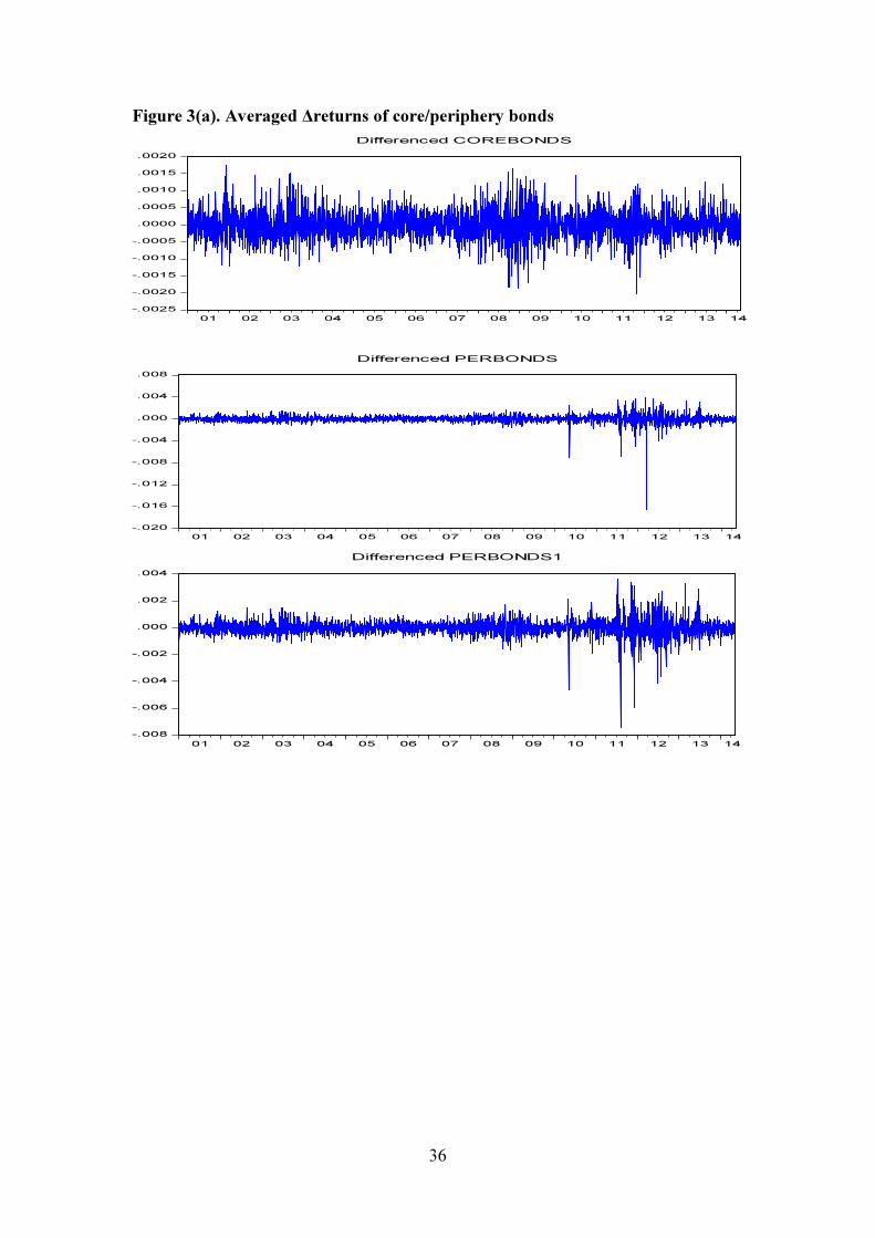
the evolution of bond yields and stock returns. In addition Figures 3(a)-(b) provide the

evolution the weighted returns of bond and stocks for the core markets, the periphery

markets with Greece and the periphery markets without Greece respectively.

The averaged bond portfolio is derived by weighting the initial bond yields

(/100). The core bond portfolio (COREBONDS) has the lowest mean return value of

0.028 on the contrary to periphery (PERBONDS, PERBONDS1 of 0.06 and 0.05

respectively. Turning to risk we observe again as expected that core bond portfolio

has the lowest risk (in terms of standard deviation) 0.004 as opposed to periphery

portfolios of 0.010 and 0.005 respectively. Core bond portfolio exhibit negative

skewnsess i.e. it is prone to more negative and extreme prices while the opposite

happens for periphery portfolios i.e. positive skewness (more extreme positive values

expected). The skewness and kurtosis deviations from the values of normal

distribution are in line with the p-value (<0.05) obtained from the Jarque-Berra

statistic. The benchmark bond market return of 10 year Overnight Interest Swap series

description is similar to core bond portfolio.

18

The mean return of averaged equity portfolio (CORESTIND) as well

periphery’s (PERSTIND) and periphery’s 1 (PERSTIND1) are negative with the first

having the lowest value. The volatility (derived from variance) is almost the same for

periphery portfolios (0.0174 and 0.0179, respectively) higher than core portfolio.

Negative skewness is also a common feature for all portfolios including the

benchmark (REUROSTOXX50). Based on the skewness, kurtosis and the p-value of

Jarque-Berra statistic we reject the null hypothesis of normality. The benchmark

return index has a mean return value among core and periphery portfolio hence we

intuitively accept its selection as an averaged index.

5. Empirical results

The first step of our analysis is to consider a window of 1 month round the

date of interest (event period 61 days; one month before and one month after the

event). In Table 5(a) we present the results for the equity returns case with the

application of the 3 different cases i.e. core stock log return index (CORESTIND) for

Germany and France, periphery stock log return index (PERSTIND) for Greece, Italy,

Ireland, Portugal and Spain and (PERSTIND1) with periphery country exempting

Greece versus the log return on EUROSTOXX50 (REUROSTOXX). We find

statistical significance (for AR t-statistic) on August 16, 2011 for the 1st case.

Furthermore, we observe that the ARs are slightly negative at the event day as

expected with marginal increase for 1 day ahead: from -0.011 to -0.004 (1st case),

from -0.004 to 0.006 (2nd

case) and from -0.006 to 0.007 (3rd

case). The market

reaction is evident for the 1st case and therefore we argue that both CEOs/investors in

Germany/France are affected. The statistical significance of the announcement of

Tobin tax is also evident in Figure 4 (Panel A) in which we observe that for the event

day there exists a statistically significant spike.

19

We then relax the hypothesis of the event period and reduce it to -10, +10 days

(21 days event period). Table 5(b) provides the estimated t-statistics and it is clear that

there is no difference in the case when we consider the absolute values whereas a

small increase in t-statistic is shown again for the 1st case. This finding leads to the

conclusion that the unexpected announcement is reflected in the returns of the (core)

equity market. 15

Therefore, we may argue that the market participants (CEOs,

investors etc.) discounted EU members’ positive position on the implantation of a

Tobin tax as a solution. Figure 5 (Panel A) provides the corresponding evolution of

the abnormal and cumulative abnormal returns for the 21 days event period and we

observe a spike for the event day only for the core markets case.

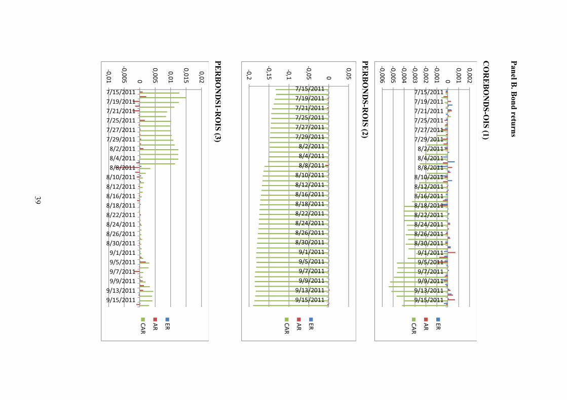
Table 5(c) provides the estimates for the bond market when we use a 61 days

period window. We find statistical significant results for the event day in the 2nd case

PERBONDS. This finding implies that the formal announcement is significant for the

market when correlated to periphery bond portfolio (with Greece included in the

sample). In addition, the 1-day ahead estimation seems to be robust to the

assumption of the positive impact on periphery countries. From Figure 4 (Panel B) we

observe that for the event day is statistical significant. For the 3rd case PERBONDS1

we observe from Figure 4 (Panel B) that the ARs of portfolio without Greece have an

extreme spike at August 8, 2011. At that date the ECB resumed its securities markets

programme (SMP) on making significant purchases of Italian and Spanish bonds for

the first time in a bid to lower yields. The AR extreme decrease is profoundly evident.

Finally, for the case of bond markets we also relax the hypothesis of the initial

61 days and reduce the event period to 21 days (10 prior, 10 after the event day).

Table 5(d) reports the respective estimates. We observe that the statistical significance

15 Cross-examining CAR t-test statistics provided the same results for both the benchmark and secondary scenario case. To save time and space we do not report CAR t-test results but focus on AR t-statistics as usual. Results are available upon request.

20

for the 2nd

case still holds. The latter is evident also from Figure 5 (Panel B) where we

observe that for the event day the spice is quite evident. We also observe that 1 day

after the announcement (1st case) significance signals under-reaction of the market.

This is also evident in Figure 5 (Panel B) on Augusts 18, 2011). Moreover the 1 day

ahead significance for 1st case signals rather a delayed under-reaction (since no

statistical significance is detected at the event day) which is also evident in Figure 5

(Panel B) for August 18, 2011. We can argue that the Tobin tax after the reduction of

the event window size (21 days) produces significant results at 5% level for both the

1st and 2

nd case.

16 For the 3rd case PERBONDS1 we observe (see Figure 5(Panel B)

as before the extreme spike at August 8, 2011 (which also evident in the PERBONDS

case).

In the second part of our analysis we estimate the chosen GARCH

specification with AR(1) conditional mean equation (Figure 6 reports the ARCH

effects in residuals of AR(1) OLS). For comparison reasons we use the same sample

as in the event study i.e. January 7, 2011 to February 8, 2012. First we model (based

on minimizing AIC criterion among competing GARCH (p,q) models) the averaged

bond yield series. For the COREBONDS series we select the GARCH(1,1) (AIC=-

12.652), for the PERBONDS series we select the GARCH(2,2) (AIC=-11.349). In

this case the dummy is significant in 5% level which is in line with the event study

results (Table 6 report the estimates)17

. Hence the announcement does affect the

volatility of the periphery return portfolio (positive sign i.e. by increasing it). For the

PERBONDS1 series (without Greece) we select again the GARCH (2,2) (AIC=-

16 Again cross-examining CAR t-test statistics provided the same results for both the benchmark and secondary scenario case. To save time and space we do not report CAR t-test results but focus on AR t-statistics as usual. Results are available upon request. 17 For sensitive analysis we also utilized the dummy depicting now a regime shift from August 16 thereafter. It proved significant at 1% significance level only for the PERBONDS case.

21

11.483) the dummy though is marginal significant (10% level). Nevertheless we state

that the variance stationarity hypothesis holds (α+β<1) for all models.

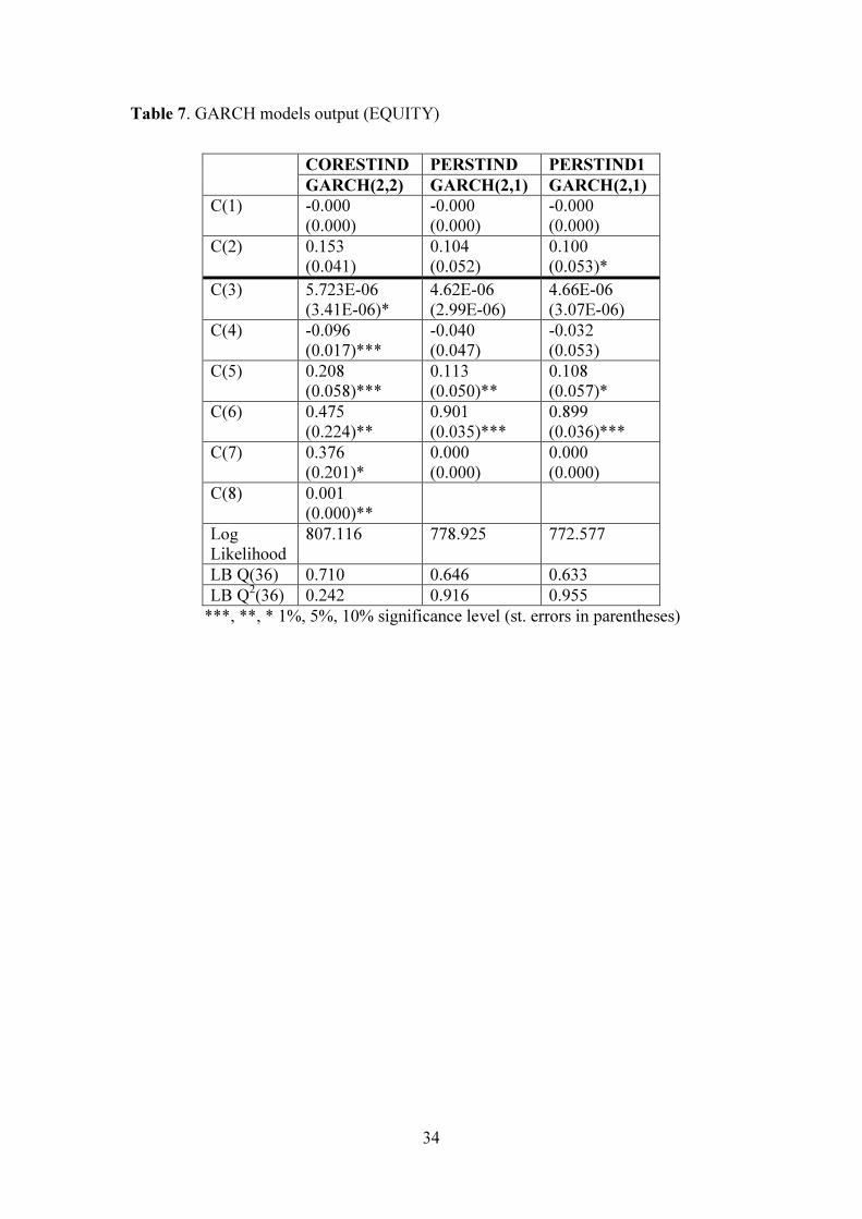
We repeat the process for equity return portfolios. We select for CORESTIND

the GARCH (2,2) model (AIC=-5.627), for PERSTINTD GARCH (2,1) (AIC=-

5.436) and PERSTINTD1 GARCH (2,1) (AIC=-5.3918). The dummy announcement

is significant with positive sign only for the first case in 5% level of significance18

.

Hence there is no benchmark comparison to the results of the event study (where we

didn’t find statistical evidence). Table 7 reports our estimates. The latter for the event

methodology results may be attributed to the positive impact to the core equity

portfolio (i.e. core EMU markets reflecting investors’ and CEOs’ expectations) by the

news. Overall, periphery bond portfolio seems to react more to news given its

association with the linked sovereign risk (countries on the verge of insolvency,

rescue packages creating debtor and creditor moral hazard). The positive sign (though

marginal) from theoretical point delivers the expected result. Nevertheless its

economic significance in conjunction to counties’ risk profile may consider it as

counter intuitive (for supporting periphery countries’ public revenues in time of the

ongoing crisis), by reflecting the uncertainty of results by the proposed regulation

mechanism. In summary, information efficiency is per se proven for those markets,

which exhibit statistical significance on the announcement day.

Finally, we argue that the positive and negative shocks induce a symmetric

response of volatility. Therefore, we show that under the announcement the EGARCH

model given the asymmetric hypothesis may fit better our purpose. We re-examine

series. COREBONDS, PERBONDS follow an EGARCH (2,2) (respectively under

AIC -12.645 and -11.388) and PERBONDS1 an EGARCH (2,1) (AIC=-11.488). The

18 For sensitive analysis we also utilized the dummy depicting now a regime shift from August 16 thereafter. It proved marginal significant at 5% significance level for the PERSTIND, PERSTIND1 cases.

22

estimated models though give mixed results (asymmetric term significant-dummy not

significant, asymmetric term significant-dummy significant, asymmetric term

significant, dummy significant). We conducted the same analysis for the equity

markets and we also obtain mixed results which implies weak evidence on our

testable hypothesis.

6. Summary and concluding remarks

The event study method produced robust results for the significance of the first

announcement on Tobin taxation on core equity return portfolios. On the contrary we

found evidence for the periphery EMU bond return portfolio case. The same was

cross-checked for the GARCH model on the same portfolio category; hence by

comparison we have a robust result. The latter may signifies that the Tobin Tax

supports more the case of financial impudent countries than the non-affected ones by

the crisis; therefore we may consider it as expected. We found also evidence for core

equity EMU under GARCH specification signaling a positive a climate towards the

implementation of the new financial regulation.

The feverish financial markets after the global financial and EMU debt crisis

are prone to extreme reactions coming from externalities outside the financial system

(unexpected events). Though the STT Tobin tax type is postponed to January 1, 2016

uncertainty looms for a greater crisis. Tools like STTs are helpful under the context of

unanimous support in order to avoid arbitrage situations. The negative response by

UK is creating a breach between the 2 major financial centers of Europe creating de

facto arbitrage pre-conditions and capital levy that in the context of semi-free capital

flows (even if the percentage is low) will re-direct capital within EU. The latter should

be taken under consideration following the expected “Brexit” referendum.

23

Generally in order to produce robust effects a Tobin tax should be

implemented as a part of a policy measures grid. As Caldari and Mansini (op. cit.)

conclude Tobin Tax approval variates between two far edges with respect to financial

conditions (appearance or not of crises): misdirected scientific criticism towards a

sudden popularization. They continue: “But if a new architecture in the world will

eventually be able to provide financial, monetary and economic stability, Tobin’s

first-best solution (a global monetary standard, which he himself considered utopian

in the 20th century) will make the second-best proposal (the tax) completely useless

and Tobin’s original intent would be vindicated” (p. 19). Nevertheless, under the

institutional spectrum of the ongoing EU/EMU debt crisis the adoption of FTTs seems

theoretically an accepted policy with expected short and long term effects for the

financial stability of EU as a consolidated economic region.

Finally, we argue that a continuous long term financial destabilization process

will lead to peripheral monetary unions in global scale due to the excessive stand

alone risk faced by a single country. In secondary level currency frictions between

unions will manifest or else the revival of protectionism over deregulated free capital

flaws will return. Thus what emerges is a clash between Markets and Governments

over regulation issues and financial dominance. FTTs as in the European case could

serve as the absorbers of future crisis events in terms of fuelling fiscal backstop funds.

24

References

Aliber R.Z., B. Chowdhry and S. Yan, 2003, Some evidence that a tobin tax on

foreign exchange transactions may increase volatility, European Finance Review, 7, p.

481-510.

Alworth J. and G.Arachi, 2010, Taxation and the financial crisis, Paper prepared for

the European Tax Policy Form / Institute for Fiscal Studies Conference: Tax Policy in

an Uncertain World, http://www.etpf.org/papers/53crisis.pdf.

Baldwin A., 2011, The Tobin tax: reason or treason, Adam Smith Institute, available

at: http://www.adamsmith.org/sites/default/files/resources/ASI_Tobin_ Tax_

2011.pdf.

Baltagi B.H, Li D. and Li Q., 2006, Transactions costs and stock market behavior:

evidence from an emerging market, Empirical Economics, 31, p. 393-408.

Becchetti L., M. Ferrari and U. Trenta, 2013, The impact of the French Tobin tax,

SSRN.

Bessebinder H. and S. Rath, 2002, Does Market Structure Matter? Trading Costs and

Return Volatility Around Exchange Listings, University of Utah, working paper.

Buiter W., 2003, James Tobin: An appreciation of his contributions to economics

(online), LSE research online, London, http://eprints.lse.ac.uk/archive/00000847.

Brunnermeier M., A. Crocket, C. Goodhart, A. Persuad and H. Sin, 2009, The

fundamental principles of financial regulation, International Center for Monetary and

Banking Studies.

Caldari K. and F. Mansini, 2010, National autonomy, regional integration and global

public goods: The debate on the Tobin Tax (1978-2009), CREI working paper no.

1/2010.

Campbell J. and K. Froot, 1994, International Experiences with Securities Transaction

Taxes, NBER.

Chou R. K. and G. H. K. Wang , 2006, transaction tax and market quality of the

Taiwan stock index futures, working paper.

Claessens S., M. Keen and C. Pazarbasioglu, 2010, Financial sector taxation. The

IMF’s report to the G-20 and background material, IMF,

http://www.taxpolicycenter.org/events/upload/IMF-studies.pdf.

Comotto R., 2013, Collateral damage: the impact of the financial transaction tax on

the European repo market and its consequences for the financial market and the real

economy”, International Capital Market Association, available at:

http://www.icmagroup.org/Regulatory-Policy-and-Market-Practice/short-termmarkets

/Repo-Markets/icma-european-repo-market-reports-and-whitepapers/theimpact-of-

the-financial-transaction-tax-on-the-european-repo-market/.

25

European Commission, 2011a, Commission Staff Working Paper: Executive

Summary of the Impact Assessment, accompanying the document, Proposal for a

Council Directive on a common system of financial transaction tax and amending

Directive 2008/7/EC, 28 September.

Damette O. (2013), Mixture distribution hypothesis and the impact of a Tobin tax on

exchange rate volatility: a reassessment, Bureau d’economie theorique et appliqué

(BETA), document de travail no. 2013-07.

Friedman M., 1953, The case of flexible exchange rates, University of Chicago Press.

Grahl J. and P. Lysandrou, 2014, The European Commission’s proposal for a

financial transaction tax: a critical assessment, Journal of Common Market Studies,

vol. 52, pp. 234-249.

Hau H., 2006, The Role of Transaction Costs for Financial Volatility: Evidence from

the Paris Bourse, Journal of the European Economic Association 4.4, pp.862-890.

Jürgen A., M. Bijlsma, A. Elbourne, M. Level and G. Swart, 2012, Financial

transaction tax: review and assessment, CPB Netherland Bureau of Economic Policy

Analysis, Discussion paper, 202.

Keynes J.M., 1936, General theory of employment, interest rates and money,

Harcourt Brace & World, Washington D.C.

Lavicka H., T. Lichard and J. Novotny, 2013, Sand in the wheels r the wheels in sans?

Tobin taxes and market crashes, Charles University Center for Economic Research

and Graduate Education, Discussion paper no. 220.

Lendvai J., R. Raciborski and L. Vogel, 2012, Securities transaction taxes:

macroeconomic implications in a general-equilibrium model, European Commission,

economic papers no. 450, available at: http://ec.europa.eu/economy_finance/

publications/economic_paper/2012/pdf/ecp_450_en.pdf

Leuz C., 2007, Was the Sarbanes-Oxley Act of 2002 really this costly?A discussion of

evidence from event returns and going-Private decisions, Journal of accounting and

Economics, 44, pp. 146-165.

Liau Y., Y. Wu and H. Hsu, 2012, Transaction tax and market volatility: evidence

from the Taiwan futures market, Journal of Applied Finance and Banking, vol.2, no.2

p.45-58.

London Economics, 2013, The impact of a financial transaction tax on corporate and

sovereign debt, report for the International Regulatory Strategy Group, City of

London Economic Development.

Masciandaro D. and F. Passarelli, 2013, Financial systemic risk: taxation or

regulation?, Journal of Banking and Finance, 37, p. 587-596.

26

Matheson T., 2012, Security transaction taxes: issues and evidence, International Tax

Public Finance, 19, p. 884-912.

McCulloch N. and G. Pacillo, 2011, The Tobin Tax- A review of the evidence,

Institute of Development Studies, University of Sussex.

McKinlay G., 1997, Event studies in Economics and Finance, Journal of Economic

Literature, vol. XXXV, p. 13-39.

McWilliams and Siegel, 1997, Event studies in Management Research: theroretical

and empirical issues, the Academy of Management Journal, vol. 40, pp. 626-657.

Phylaktis K. and A. Aristidou, 2007, Security transaction taxes and financial

volatility: Athens Stock Exchange, Applied Financial Economics, 17:18, p. 1455-

1467.

Pomeranets A., 2013, Securities Transaction Taxes: Literature and key issues,

Encyclopedia of Finance, p. 777-781, available at: http://link.springer.com/

referenceworkentry/10.1007%2F978-1-4614-5360-4_66.

Posner E. and G. Weyl, 2013, Benefit-cost analysis for financial regulation, SSRN,

available at: http://papers.ssrn.com/sol3/papers.cfm?abstract_id=2188990.

Ross S., 1989, Commentary [on Stiglitz 1989], Journal of Financial Services Research

3, p. 117-120.

Roll R., 1989, Price Volatility, International Market Links and Their Implication for

Regulatory Policies, Journal of Financial Services Research, Vol. 3(2-3), pp. 211-246.

Sanger G.S., C.F. Sirmans and G.K. Turnbull, 1990, The effects of tax reform on real

estate: some empirical results, Land Economics, 66, p.409-424.

Saporta V. and K. Kan, 1997, The Effects of Stamp Duty on the Level and Volatility

of Equity Prices, Bank of England Working Paper No. 71.

Schulmeister S., M. Schratzenstaller, and O. Picek, 2008, A General Financial

Transaction Tax: Motives, Revenues, Feasibility and Effects, Oesterreichisches

Institut fuer Wirtschaftsforschung working paper, Vienna.

Schwert G.W., and P. Seguin, 1993, Securities Transaction Taxes: an Overview of

Costs, Benefits and Unresolved Questions, Financial Analysts Journal, September-

October, pp. 27–35.

Shaviro D., 2012, The financial transactions tax versus (?) the financial activity tax,

New York University Law and Economics, Working Paper 292,

http://lsr.nellco.org/nuy_lewp/292.

Stiglitz J., (1989): “Using Tax Policy to Curb Speculative Short-Term Trading,”

Journal of Financial Services Research, Vol. 3(2-3), pp. 101–15.

27

Stiroh K. (2010): “Why are some banks systemically important? What we do about

it?”, Federal Bank of New York, http://www.imf.org/external/np/seminars/eng/2010

/mcm/pdf/KStiroh.pdf.

Summers L., and Summers V. (1989): “When Financial Markets Work Too Well: A

Cautious Case for a Securities Transaction Tax,” Journal of Financial Services

Research, Vol. 3, pp. 261–86.

Tobin J., 1978, A Proposal for International Monetary Reform, The Eastern Economic

Journal, 4, 153-159.

Umlauf S., 1993, Transaction Taxes and the Behavior of the Swedish Stock Market,

Journal of Financial Economics, Vol. 33, pp. 227–40.

Uppal R., 2011, A short note on the Tobin Tax: The costs and benefits of a tax on

financial transaction, EDHEC- Risk Institute.

28

Table 1. Negative externalities and solutions for systemic risk

Solution Examples for Systemic

Risk

“Pigouvian” tax Tax on bank leverage

Activity restrictions Restrict proprietary trading

Subsidize actions Subsidize bank capital

Tradable permits Trade right to breach

capital requirement

Reduce externality Exposure limits

Clean up ex post Asset guarantees

Source: Stiroh (2010)

Table 2. Selected theoretical and empirical models on Tobin Tax and Volatility.

AUTHOR(S) IMPACT OF TOBIN TAX ON VOLATILITY

Hanke et al. (2010)

Increase or decrease depending on market size

Shi and Hu (2009) Increase or decrease depending on the effect on

the number of noise traders

Westerhoff (2003) and Westerhoff and Dieci

(2006)

Decrease

Ehrenstein (2002, 2005)

Decrease, as long as the tax rate is not too high to affect the liquidity

Mannaro et al. (2008) Increase, but only in presence of noise traders in the market

Kaiser et al. (2007) Decrease

Bianconi et al. (2009) Decrease but depending on market size

Bloomfield et al. (2009) Little effect on volatility

Hau (2008) Decrease

Pellizzari and Westerhoff (2009) Decrease in highly liquid dealership markets; no effect in limit order markets

Source: McCulloch and Pacillo, 2011.

29

Table 3. Weights for averaged returns (equity/bonds) series

Country level Series Weights

Core

Eurozone

CORECDS

Germany GECDS 0.58

France FRCDS 0.42

Periphery

Eurozone

PERCDS

Greece GRCDS 0.058

Ireland IRCDS 0.052(0.056)

Italy ITCDS 0.504(0.536)

Portugal PCDS 0.050(0.056)

Spain SPCDS 0.330(0.352)

Note: Countries’ CDS are averaged based on their GDP (2012). The selection of the year 2012 depicts real economy performance for countries and not diluting effects on their overall performance (crisis correction). EMU periphery for calculation purposes are grouped twice; once including and the second excluding Greece as the ground zero of the euro debt crisis (weights in parentheses).

30

Table 4. Descriptive statistics

Bond yields

GE10Y_ FR10Y_ GR10Y_ IR10Y_ IT10Y_ P10Y_ SP10Y_

Mean 0.034 0.036 0.079 0.048 0.044 0.054 0.044

Max. 0.052 0.053 0.486 0.138 0.072 0.162 0.075

Min. 0.011 0.016 0.032 0.028 0.031 0.029 0.030

Std. Dev. 0.010 0.008 0.069 0.016 0.006 0.023 0.007

Skewness -0.502 -0.296 2.612 2.030 0.862 1.984 0.750

Kurtosis 2.194 2.425 10.092 7.486 4.261 6.302 3.467

JarqueJarque- Bera 240.722 98.654 11245.86 5306.973 662.105 3864.189 358.260

Prob. 0.000 0.000 0.000 0.000 0.000 0.000 0.000

Obs. 3478 3478 3478 3478 3478 3478 3478

Weighted bond yield series (portfolios)

COREBONDS PERBONDS PERBONDS1 OIS10Y_

Mean 0.028744 0.068482 0.059276 0.026039

Max. 0.036197 0.091325 0.075217 0.034810

Min. 0.020588 0.054091 0.050569 0.017419

Std. Dev. 0.004487 0.010600 0.005888 0.004986

Skewness -0.063691 0.635901 0.659678 -0.149438

Kurtosis 1.510.802 2.068.107 2.313.899 1.441.008

Jarque- Bera 2.680.723 2.983.085 2.653.724 3.023.738

Prob. 0.000002 0.000000 0.000002 0.000000

Obs. 288 288 288 288

31

Equity indices

REUROSTOXX RMDAX RCAC40 RATHEX RFTSEMIB RIGBM RISEQ RPSI*

Mean 6.59E-05 0.000 8.45E-05 -0.000 -8.67E-05 0.000 -2.03E-05 2.30E-05

Max. 0.104 0.112 0.105 0.134 0.108 0.137 0.097 0.097

Min. -0.082 -0.090 -0.094 -0.102 -0.085 -0.096 -0.139 -0.106

Std. Dev. 0.014 0.014 0.014 0.018 0.015 0.014 0.015 0.011

Skewness 0.016 -0.258 0.050 -0.007 -0.070 0.153 -0.599 -0.136

Kurtosis 9.757 8.319 10.203 6.832 8.679 10.480 11.003 14.332

Jarque -Bera 4943.291 3092.261 5618.051 1590.034 3494.065 6067.160 7090.346 13910.76

Prob. 0.000 0.000 0.000 0.000 0.000 0.000 0.000 0.000

Obs. 2598 2598 2598 2598 2598 2598 2598 2598

*common sample 2598obs. (PSI start 17/5/2004)

Weighted series (equity return portfolios)

CORESTIND PERSTIND PERSTIND1 REUROSTOXX50

Mean -0.000128 -0.000619 -0.000532 -0.000367

Max. 0.051953 0.049467 0.049648 0.058981

Min. -0.059886 -0.057887 -0.059032 -0.063184

Std. Dev. 0.016868 0.017457 0.017908 0.017485

Skewness -0.293250 -0.304553 -0.303507 -0.172220

Kurtosis 4.737.005 3.851.232 3.821.974 4.469.355

Jarque- Bera 4.033.404 1.314.726 1.252.928 2.733.170

Prob. 0.000000 0.001397 0.001902 0.000001

Obs. 288 288 288 288

32

Table 5(a). Abnormal returns for equities – 61 days event period

1st case 2

nd case 3

rd case

day AR t-stat AR t-stat AR t-stat

-1 1.065 -0.664 -0.675

0 -3.004 -1.029 -1,485

+1 -1.046 1.430 1,633

Note: Numbers in bold indicate statistical significance at the 5% critical value.

Table 5(b). Abnormal returns for equities – 21 days event period

1st case 2

nd case 3

rd case

day AR t-stat AR t-stat AR t-stat

-1 1.076 -0.613 -0.623

0 -3.073 -0.941 -1.359

+1 -1.077 1.469 1.609

Table 5(c). Abnormal returns for bonds – 61 days event period

1st case 2

nd case 3

rd case

day AR t-stat AR t-stat AR t-stat

-1 -0.055 -1.638 0.008

0 0.007 -2.407 -0.441

+1 -0.221 -2.875 -1.415

Table 5(d). Abnormal returns for equities – 21 days event period

1st case 2

nd case 3

rd case

day AR t-stat AR t-stat AR t-stat

-1 -0.584 0.215 0.049

0 0.028 -2,463 -0,455

+1 -2.266 -3,993 -1,330

33

Table 6. GARCH models output (BONDS)

COREBONDS PERBONDS PERBONDS1

GARCH(1,1) GARCH(2,2) GARCH(2,2)

C(1) -2.878

(3.18E-05)

7.91E-05

(4.26E-05)*

4.02E-05

(3.51E-05)

C(2) 0.267

(0.060)***

0.321

(0.062)***

0.272

(0.055)***

C(3) 4.352

(3.66E-09)

1.343E-07

(2.13E-

08)***

9.30E-08

(1.93E-08)***

C(4) 0.064

(0.029)**

0.332

(0.143)**

0.426

(0.162)***

C(5) 0.907

(0.034)***

0.189

(0.184)

0.179

(0.198)

C(6) 2.845E-07

(1.98E-07)

0.451

(0.084)***

0.485

(0.047)***

C(7) -0.095

(0.022)***

-0.105

(0.012)***

C(8) 4.75E-05

(2.33E-05)**

4.58E-05

(2.49E-05)*

Log

Likelihood

1802.655 1626.178 1638.25

LB Q(36) 0.484 0.545 0.830

LB Q2(36) 0.529 0.977 0.875

***, **, * 1%, 5%, 10% significance level (st. errors in parentheses)

C(1), C(2) conditional mean equation parameters

C(3) conditional variance constant

C(4) (C(4)-C(5)) arch terms, C(5) (C(6)-C(7))garch terms

C(6) (C(8))dummy coefficient

34

Table 7. GARCH models output (EQUITY)

CORESTIND PERSTIND PERSTIND1

GARCH(2,2) GARCH(2,1) GARCH(2,1)

C(1) -0.000

(0.000)

-0.000

(0.000)

-0.000

(0.000)

C(2) 0.153

(0.041)

0.104

(0.052)

0.100

(0.053)*

C(3) 5.723E-06

(3.41E-06)*

4.62E-06

(2.99E-06)

4.66E-06

(3.07E-06)

C(4) -0.096

(0.017)***

-0.040

(0.047)

-0.032

(0.053)

C(5) 0.208

(0.058)***

0.113

(0.050)**

0.108

(0.057)*

C(6) 0.475

(0.224)**

0.901

(0.035)***

0.899

(0.036)***

C(7) 0.376

(0.201)*

0.000

(0.000)

0.000

(0.000)

C(8) 0.001

(0.000)**

Log

Likelihood

807.116 778.925 772.577

LB Q(36) 0.710 0.646 0.633

LB Q2(36) 0.242 0.916 0.955

***, **, * 1%, 5%, 10% significance level (st. errors in parentheses)

35

Figure 1. Bond yields for core and periphery EMU (levels)

0

10

20

30

40

50

01 02 03 04 05 06 07 08 09 10 11 12 13 14

FR10Y GE10Y GR10Y

IR10Y IT10Y P10Y

SP10Y

Figure 2. Stock price indexes

6

7

8

9

10

11

01 02 03 04 05 06 07 08 09 10 11 12 13 14

Log EUROSTOXX50 Log MDAX

Log CAC40 Log ATHEX

Log FTSEMIB Log IGBM

Log ISEQ Log PSI

36

Figure 3(a). Averaged Δreturns of core/periphery bonds

-.0025

-.0020

-.0015

-.0010

-.0005

.0000

.0005

.0010

.0015

.0020

01 02 03 04 05 06 07 08 09 10 11 12 13 14

Differenced COREBONDS

-.020

-.016

-.012

-.008

-.004

.000

.004

.008

01 02 03 04 05 06 07 08 09 10 11 12 13 14

Differenced PERBONDS

-.008

-.006

-.004

-.002

.000

.002

.004

01 02 03 04 05 06 07 08 09 10 11 12 13 14

Differenced PERBONDS1

37

Figure 3(b). Averaged Δlog returns of core/periphery equity indices

-.12

-.08

-.04

.00

.04

.08

.12

01 02 03 04 05 06 07 08 09 10 11 12 13 14

CORESTIND

-.12

-.08

-.04

.00

.04

.08

.12

01 02 03 04 05 06 07 08 09 10 11 12 13 14

PERSTIND

-.12

-.08

-.04

.00

.04

.08

.12

01 02 03 04 05 06 07 08 09 10 11 12 13 14

PERSTIND1

38

Fig

ure 4

. Ab

norm

al (A

R) a

nd

Cu

mu

lativ

e ab

norm

al re

turn

s (CA

R)

(61 d

ays ev

ent p

eriod

)

Pan

el A. E

qu

ity retu

rns

CO

RE

ST

IND

-RE

UR

OS

TO

XX

(1)

PE

RS

TIN

D-R

EU

RO

ST

OX

X (2

)

PE

RS

TIN

D1-R

EU

RO

ST

OX

X (3

)

-0,1

-0,08

-0,06

-0,04

-0,02 0

0,02

0,04

0,06

7/15/2011

7/19/2011

7/21/2011

7/25/2011

7/27/2011

7/29/2011

8/2/2011

8/4/2011

8/8/2011

8/10/2011

8/12/2011

8/16/2011

8/18/2011

8/22/2011

8/24/2011

8/26/2011

8/30/2011

9/1/2011

9/5/2011

9/7/2011

9/9/2011

9/13/2011

9/15/2011

ER

AR

CAR

-0,08

-0,06

-0,04

-0,02 0

0,02

0,04

0,06

7/15/2011

7/19/2011

7/21/2011

7/25/2011

7/27/2011

7/29/2011

8/2/2011

8/4/2011

8/8/2011

8/10/2011

8/12/2011

8/16/2011

8/18/2011

8/22/2011

8/24/2011

8/26/2011

8/30/2011

9/1/2011

9/5/2011

9/7/2011

9/9/2011

9/13/2011

9/15/2011

ER

AR

CAR

-0,08

-0,06

-0,04

-0,02 0

0,02

0,04

0,06

7/15/2011

7/19/2011

7/21/2011

7/25/2011

7/27/2011

7/29/2011

8/2/2011

8/4/2011

8/8/2011

8/10/2011

8/12/2011

8/16/2011

8/18/2011

8/22/2011

8/24/2011

8/26/2011

8/30/2011

9/1/2011

9/5/2011

9/7/2011

9/9/2011

9/13/2011

9/15/2011

ER

AR

CAR

39

Pan

el B. B

on

d retu

rns

CO

RE

BO

ND

S-O

IS (1

)

PE

RB

ON

DS

-RO

IS (2

)

PE

RB

ON

DS

1-R

OIS

(3)

-0,006

-0,005

-0,004

-0,003

-0,002

-0,001 0

0,001

0,002

7/15/2011

7/19/2011

7/21/2011

7/25/2011

7/27/2011

7/29/2011

8/2/2011

8/4/2011

8/8/2011

8/10/2011

8/12/2011

8/16/2011

8/18/2011

8/22/2011

8/24/2011

8/26/2011

8/30/2011

9/1/2011

9/5/2011

9/7/2011

9/9/2011

9/13/2011

9/15/2011

ER

AR

CAR

-0,2

-0,15

-0,1

-0,05 0

0,05

7/15/2011

7/19/2011

7/21/2011

7/25/2011

7/27/2011

7/29/2011

8/2/2011

8/4/2011

8/8/2011

8/10/2011

8/12/2011

8/16/2011

8/18/2011

8/22/2011

8/24/2011

8/26/2011

8/30/2011

9/1/2011

9/5/2011

9/7/2011

9/9/2011

9/13/2011

9/15/2011

ER

AR

CAR

-0,01

-0,005 0

0,005

0,01

0,015

0,02

7/15/2011

7/19/2011

7/21/2011

7/25/2011

7/27/2011

7/29/2011

8/2/2011

8/4/2011

8/8/2011

8/10/2011

8/12/2011

8/16/2011

8/18/2011

8/22/2011

8/24/2011

8/26/2011

8/30/2011

9/1/2011

9/5/2011

9/7/2011

9/9/2011

9/13/2011

9/15/2011

ER

AR

CAR

40

Gra

ph

.5 A

bn

orm

al (A

R) a

nd

Cu

mu

lativ

e ab

norm

al re

turn

s (CA

R)

(21 d

ays ev

ent p

eriod

)

Pan

el A. E

qu

ity retu

rns

-0,08

-0,06

-0,04

-0,02 0

0,02

0,04

8/2/2011

8/3/2011

8/4/2011

8/5/2011

8/8/2011

8/9/2011

8/10/2011

8/11/2011

8/12/2011

8/15/2011

8/16/2011

8/17/2011

8/18/2011

8/19/2011

8/22/2011

8/23/2011

8/24/2011

8/25/2011

8/26/2011

8/29/2011

8/30/2011

AR(1)

CAR(1)

-0,02

-0,01 0

0,01

0,02

0,03

0,04

8/2/2011

8/3/2011

8/4/2011

8/5/2011

8/8/2011

8/9/2011

8/10/2011

8/11/2011

8/12/2011

8/15/2011

8/16/2011

8/17/2011

8/18/2011

8/19/2011

8/22/2011

8/23/2011

8/24/2011

8/25/2011

8/26/2011

8/29/2011

8/30/2011

AR(2)

CAR(2)

-0,02 0

0,02

0,04

8/2/2011

8/3/2011

8/4/2011

8/5/2011

8/8/2011

8/9/2011

8/10/2011

8/11/2011

8/12/2011

8/15/2011

8/16/2011

8/17/2011

8/18/2011

8/19/2011

8/22/2011

8/23/2011

8/24/2011

8/25/2011

8/26/2011

8/29/2011

8/30/2011

AR(3)

CAR(3)

41

Pan

el B. Β

on

d retu

rns

-0,006

-0,004

-0,002 0

0,002

8/2/2011

8/3/2011

8/4/2011

8/5/2011

8/8/2011

8/9/2011

8/10/2011

8/11/2011

8/12/2011

8/15/2011

8/16/2011

8/17/2011

8/18/2011

8/19/2011

8/22/2011

8/23/2011

8/24/2011

8/25/2011

8/26/2011

8/29/2011

8/30/2011

AR(1)

CAR(1)

-0,2

-0,15

-0,1

-0,05 0

0,05

7/15/2011

7/19/2011

7/21/2011

7/25/2011

7/27/2011

7/29/2011

8/2/2011

8/4/2011

8/8/2011

8/10/2011

8/12/2011

8/16/2011

8/18/2011

8/22/2011

8/24/2011

8/26/2011

8/30/2011

9/1/2011

9/5/2011

9/7/2011

9/9/2011

9/13/2011

9/15/2011

AR(2)

CAR(2)

-0,01 0

0,01

0,02

7/15/2011

7/19/2011

7/21/2011

7/25/2011

7/27/2011

7/29/2011

8/2/2011

8/4/2011

8/8/2011

8/10/2011

8/12/2011

8/16/2011

8/18/2011

8/22/2011

8/24/2011

8/26/2011

8/30/2011

9/1/2011

9/5/2011

9/7/2011

9/9/2011

9/13/2011

9/15/2011

AR(3)

CAR(3)

42

Graph 6. Residual graphs AR(1) OLS (bond Δyields 10y).

-.003

-.002

-.001

.000

.001

.002

.003

01 02 03 04 05 06 07 08 09 10 11 12 13 14

D(FR10Y_) Residuals

-.003

-.002

-.001

.000

.001

.002

01 02 03 04 05 06 07 08 09 10 11 12 13 14

D(GE10Y_) Residuals

-.012

-.008

-.004

.000

.004

.008

01 02 03 04 05 06 07 08 09 10 11 12 13 14

D(IR10Y_) Residuals

-.008

-.006

-.004

-.002

.000

.002

.004

.006

01 02 03 04 05 06 07 08 09 10 11 12 13 14

D(IT10Y_) Residuals

-.016

-.012

-.008

-.004

.000

.004

.008

.012

.016

.020

01 02 03 04 05 06 07 08 09 10 11 12 13 14

D(P10Y_) Residuals

-.010

-.008

-.006

-.004

-.002

.000

.002

.004

01 02 03 04 05 06 07 08 09 10 11 12 13 14

D(SP10Y_) Residuals

-.28

-.24

-.20

-.16

-.12

-.08

-.04

.00

.04

.08

01 02 03 04 05 06 07 08 09 10 11 12 13 14

D(GR10Y_) Residuals

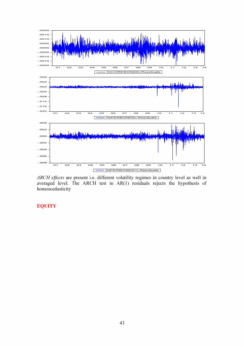
43

-.0020

-.0015

-.0010

-.0005

.0000

.0005

.0010

.0015

.0020

01 02 03 04 05 06 07 08 09 10 11 12 13 14

D(COREBONDS) Residuals

-.020

-.016

-.012

-.008

-.004

.000

.004

.008

01 02 03 04 05 06 07 08 09 10 11 12 13 14

D(PERBONDS) Residuals

-.008

-.006

-.004

-.002

.000

.002

.004

01 02 03 04 05 06 07 08 09 10 11 12 13 14

D(PERBONDS1) Residuals

ARCH effects are present i.e. different volatility regimes in country level as well in

averaged level. The ARCH test in AR(1) residuals rejects the hypothesis of

homoscedasticity

EQUITY