Field and Numerical Investigation to Determine the Impact ...

Field and Numerical Investigation to Determine the Impact of Environmental and Wheel Loads on Flexible Pavement

by

Alireza Bayat

A thesis presented to the University of Waterloo

in fulfillment of the thesis requirement for the degree of

Doctor of Philosophy in

Civil Engineering

Waterloo, Ontario, Canada, 2009 © Alireza Bayat 2009

ii

AUTHOR'S DECLARATION I hereby declare that I am the sole author of this thesis. This is a true copy of the thesis, including any required final revisions, as accepted by my examiners. I understand that my thesis may be made electronically available to the public.

iii

Abstract There is a growing interest for the use of mechanistic procedures and analytical methods in the

design and evaluation of pavement structure rather than empirical design procedures. The

mechanistic procedures rely on predicting pavement response under traffic and environmental

loading (i.e., stress, strain, and deflection) and relating these responses to pavement field

performance.

A research program has been developed at the Center for Pavement and Transportation

Technology (CPATT) test track to investigate the impact of traffic and environmental parameters

on flexible pavement response. This unique facility, located in a climate with seasonal

freeze/thaw events, is equipped with an internet accessible data acquisition system capable of

reading and recording sensors using a high sampling rate. A series of controlled loading tests

were performed to investigate pavement dynamic response due to various loading configurations.

Environmental factors and pavement performance were monitored over a two-year period.

Analyses were performed using the two dimensional program MichPave to predict pavement

responses. The dynamic modulus test was chosen to determine viscoelastic properties of Hot Mix

Asphalt (HMA) material. A three-step procedure was implemented to simplify the incorporation

of laboratory determined viscoelastic properties of HMA into the finite element (FE) model. The

FE model predictions were compared with field measured pavement response.

Field test results showed that pavement fully recovers after each wheel pass. Wheel wander and

asphalt mid-depth temperature changes were found to have significant impact on asphalt

longitudinal strain. Wheel wander of 16 cm reduced asphalt longitudinal strains by 36 percent

and daily temperature fluctuations can double the asphalt longitudinal strain.

iv

Results from laboratory dynamic modulus tests found that Hot Laid 3 (HL3) dynamic modulus is

an exponential function of the test temperature when loading frequency is constant, and that the

HL3 dynamic modulus is a non-linear function of the loading frequency when the test

temperature is constant. Results from field controlled wheel load tests found that HL3 asphalt

longitudinal strain is an exponential function of asphalt mid-depth temperature when the truck

speed and wheel loading are constant. This indicated that the laboratory measured dynamic

modulus is inversely proportional to the field measured asphalt longitudinal strain.

Results from MichPave finite element program demonstrated that a good agreement between

field measured asphalt longitudinal strain and MichPave prediction exists when field represented

dynamic modulus is used as HMA properties.

Results from environmental monitoring found that soil moisture content and subgrade resilient

modulus changes in the pavement structure have a strong correlation and can be divided into

three distinct Seasonal Zones. Temperature data showed that the pavement structure went

through several freeze-thaw cycles during the winter months. Daily asphalt longitudinal strain

fluctuations were found to be correlated with daily temperature changes and asphalt longitudinal

strain fluctuations as high as 650m/m were recorded. The accumulation of irrecoverable

asphalt longitudinal strain was observed during spring and summer months and irrecoverable

asphalt longitudinal strain as high as 2338m/m was recorded.

v

Acknowledgments

I would like to express my sincere appreciation to my supervisor, Dr. Mark Knight, for all the

patience, encouragement, and support I received during my study. I am very grateful to Dr.

Knight who gave me complete freedom to explore on my own and at the same time provided

watchful guidance whenever required. Thank you for all your support.

I would also like to thank my co-supervisor Dr. Leo Rothenburg for his invaluable advice

excellent feedback and for sharing his experience. Special thanks to Dr. Ralph Haas for his help

and support. I would also like to thank my examining committee members, Dr. Curtis Berthelot,

Dr. Giovanni Cascante, Dr. Maurice Dusseault, and Dr. Carl Haas for reviewing this thesis and

their advice.

This research would not have been possible without financial support from NSERC, CATT,

CPATT, MTO, and the University of Waterloo. I appreciate the support of these institutions. I

would also like to acknowledge the University of Waterloo technical staff, Mr. Ken Bowman and

Mr. Terry Ridgway for their assistance. Also, I would like to express my appreciation to Ms.

Alice Seviora for her help and assistance for finalizing the thesis manuscript. I thank my friends

and colleagues in the Geotechnical laboratory Mr. Rizwan Younis, Mr. Rashid Rehan, and Dr.

Ademola Adedapo for their friendship and help. Special thanks to Mr. Karl Lawrence and Ms.

Colleen Ryan for their friendship and support and making my stay in Waterloo unforgettable.

Finally, I want to thank my wife and best friend, Fatemeh, my parents, my brother, and my sister

for their love and persistent support in pursuing my educational goals.

vi

Dedication

To my wife, Fatemeh, and my parents

vii

Table of Contents

LIST OF TABLES .................................................................................................................... XII

LIST OF FIGURES .................................................................................................................XIII

1 INTRODUCTION ................................................................................................................ 1

1.1 PROBLEM STATEMENT ..................................................................................................... 2

1.2 RESEARCH OBJECTIVES ................................................................................................... 4

1.3 THESIS ORGANIZATION.................................................................................................... 5

2 BACKGROUND AND LITERATURE REVIEW ............................................................ 7

2.1 PAVEMENT DESIGN METHODS ......................................................................................... 8

2.1.1 AASHTO Design Method ............................................................................................ 8

2.1.2 Mechanistic-Empirical (M-E) Design Method ........................................................... 9

2.2 PAVEMENT ANALYSIS METHODS................................................................................... 12

2.2.1 Single Layer Model ................................................................................................... 12

2.2.2 Layered Elastic Theory ............................................................................................. 14

2.2.3 Finite Element Analysis ............................................................................................ 16

2.3 PAVEMENT MATERIAL CHARACTERIZATION.................................................................. 17

2.3.1 HMA Material........................................................................................................... 17

2.3.2 Unbound Material..................................................................................................... 19

2.4 FULL-SCALE INSTRUMENTED TEST FACILITIES.............................................................. 21

2.4.1 Penn State Test Track ............................................................................................... 22

2.4.2 Minnesota Road (MnRoad)....................................................................................... 22

2.4.3 Virginia Smart Road ................................................................................................. 23

2.4.4 Ohio Test Track......................................................................................................... 24

2.5 VALIDATION OF RESPONSE MODELS WITH FIELD MEASURED PAVEMENT RESPONSE.... 24

2.6 ENVIRONMENTAL IMPACTS ON PAVEMENT RESPONSE AND PERFORMANCE .................. 28

3 FLEXIBLE PAVEMENT RESPONSE UNDER DYNAMIC WHEEL LOADS-A

CPATT FULL-SCALE INSTRUMENTED TEST ROAD STUDY ............................. 31

3.1 OVERVIEW ..................................................................................................................... 32

viii

3.2 INTRODUCTION .............................................................................................................. 33

3.3 CPATT TEST TRACK..................................................................................................... 34

3.3.1 Site Information ........................................................................................................ 34

3.3.2 Field Monitoring Program ....................................................................................... 36

3.3.3 Data Acquisition ....................................................................................................... 40

3.3.4 Power Supply and Management ............................................................................... 41

3.3.5 Remote Monitoring System ....................................................................................... 42

3.3.6 Instrumentation Survivability.................................................................................... 43

3.4 2006 FIELD TESTING PROGRAM..................................................................................... 43

3.5 DATA COLLECTION AND ANALYSIS ............................................................................... 46

3.5.1 Impact of Wheel Wander on Asphalt Strain Gauge Response.................................. 49

3.5.2 Effect of Temperature on Measured Longitudinal Strains ....................................... 51

3.6 SUMMARY AND CONCLUSIONS....................................................................................... 53

3.7 ACKNOWLEDGMENT ...................................................................................................... 54

4 ALIDATION OF HOT-MIX ASPHALT DYNAMIC MODULUS USING FIELD

MEASURED PAVEMENT RESPONSE......................................................................... 55

4.1 OVERVIEW ..................................................................................................................... 56

4.2 INTRODUCTION .............................................................................................................. 57

4.3 DYNAMIC MODULUS TEST............................................................................................. 58

4.3.1 Changes in Dynamic Modulus with Temperature .................................................... 59

4.3.2 Changes in Dynamic Modulus with Frequency ........................................................ 61

4.4 CPATT FIELD TEST FACILITY ....................................................................................... 63

4.5 FIELD TESTING PROGRAM.............................................................................................. 64

4.5.1 Effect of Temperature on Measured Asphalt Longitudinal Strains .......................... 66

4.5.2 Effect of Truck Speed on Measured Asphalt Longitudinal Strains ........................... 69

4.5.3 Truck Speed and Loading Frequency ....................................................................... 70

4.6 COMPARISON OF DYNAMIC MODULUS TEST TO PAVEMENT FIELD RESPONSE............... 72


4.8 ACKNOWLEDGMENT ...................................................................................................... 74

ix

5 INVESTIGATION OF FLEXIBLE PAVEMENT STRUCTURAL RESPONSE FOR

THE CENTRE FOR PAVEMENT AND TRANSPORTATION TECHNOLOGY

(CPATT) TEST ROAD ..................................................................................................... 75

5.1 OVERVIEW ..................................................................................................................... 76

5.2 INTRODUCTION .............................................................................................................. 77

5.3 CPATT FIELD TEST FACILITY ....................................................................................... 78

5.4 FIELD TESTING PROGRAM.............................................................................................. 79

5.5 FINITE ELEMENT (FE) MODELING ................................................................................. 87

5.5.1 Model Formulation and Assumptions....................................................................... 87

5.5.2 HMA Modulus Characterization............................................................................... 89

5.5.3 Granular Material Characterization ........................................................................ 93

5.6 VALIDATION OF THE FE MODEL..................................................................................... 95


5.8 ACKNOWLEDGEMENTS................................................................................................... 99

6 LONG-TERM MONITORING OF ENVIRONMENTAL PARAMETERS TO

INVESTIGATE FLEXIBLE PAVEMENT RESPONSE ............................................ 100

6.1 OVERVIEW ................................................................................................................... 101

6.2 INTRODUCTION ............................................................................................................ 102

6.3 SITE INFORMATION ...................................................................................................... 104

6.4 DATA COLLECTION ...................................................................................................... 105

6.4.1 Sensors .................................................................................................................... 105

6.4.2 Data Acquisition Systems (DAS)............................................................................. 108

6.4.3 Power Supply and Management ............................................................................. 109

6.4.4 Remote Monitoring System ..................................................................................... 110

6.4.5 Pavement Response Surveys ................................................................................... 111

6.5 DATA PROCESSING....................................................................................................... 112

6.6 DATA ANALYSIS .......................................................................................................... 113

6.6.1 Ground and Ambient Air Temperature Variation................................................... 113

6.6.2 Average Daily Temperature.................................................................................... 116

6.6.3 Moisture Content Variation over Monitoring Period............................................. 117

x

6.6.4 Moisture and Pavement Performance Variation with Time ................................... 119

6.6.5 Thermal Induced Strain .......................................................................................... 120

6.7 CONCLUSIONS.............................................................................................................. 121

6.8 ACKNOWLEDGEMENT .................................................................................................. 123

7 OBSERVED SEASONAL VARIATION OF ENVIRONMENTAL FACTORS AND

THEIR IMPACT ON FLEXIBLE PAVEMENT PERFORMANCE SUBJECT TO

ANNUAL FREEZE/ THAW........................................................................................... 124

7.1 OVERVIEW ................................................................................................................... 125

7.2 INTRODUCTION ............................................................................................................ 126

7.3 CPATT TEST TRACK................................................................................................... 127

7.4 DATA COLLECTION SYSTEM ........................................................................................ 128

7.4.1 Pavement Instrumentation ...................................................................................... 128

7.4.2 Meteorological Data............................................................................................... 130

7.4.3 Pavement Performance Surveys ............................................................................. 130

7.5 MOISTURE CONTENT VARIATION DURING MONITORING PERIOD................................. 130

7.6 PAVEMENT TEMPERATURE VARIATION OVER MONITORING PERIOD ........................... 131

7.6.1 Average Monthly Temperature Distribution........................................................... 133

7.7 SEASONAL ZONES ........................................................................................................ 135

7.8 MOISTURE AND PAVEMENT PERFORMANCE VARIATION OVER MONITORING PERIOD.. 138

7.9 SUMMARY AND CONCLUSIONS..................................................................................... 141

7.10 ACKNOWLEDGEMENT .................................................................................................. 142

8 MEASUREMENT AND ANALYSIS OF FLEXIBLE PAVEMENT THERMAL-

INDUCED STRAINS....................................................................................................... 143

8.1 OVERVIEW ................................................................................................................... 144

8.2 INTRODUCTION ............................................................................................................ 145

8.3 CPATT FIELD TEST FACILITY ..................................................................................... 146

8.3.1 Site Information ...................................................................................................... 146

8.3.2 Instrumentation ....................................................................................................... 147

8.3.3 Thermal-Induced Strain-2004................................................................................. 148

8.3.4 Daily Thermal-Induced Strain Fluctuation ............................................................ 151

xi

8.3.5 Thermal-Induced Strain and Temperature below the Asphalt................................ 153

8.3.6 Thermal Induced Strain- 2005 ................................................................................ 154

8.3.7 2004-2006 Asphalt Strain Gauge............................................................................ 155

8.4 SUMMARY AND CONCLUSIONS..................................................................................... 159

8.5 ACKNOWLEDGEMENTS................................................................................................. 160

9 CONCLUSIONS AND RECOMMENDATIONS.......................................................... 161

9.1 GENERAL SUMMARY.................................................................................................... 162

9.2 CONCLUSIONS.............................................................................................................. 163

9.3 RECOMMENDATIONS AND FUTURE WORK ................................................................... 166

REFERENCES.......................................................................................................................... 168

xii

List of Tables

Table 2-1: Boussinesq’s Equations for a Point Load (after Ullidtz 1998)........................ 14

Table 2-2:Test Facilities Active since 1962 (Hamad 2007) ............................................. 23

Table 4-1: HL3 Dynamic Modulus................................................................................... 59

Table 4-2: a, b and R2 Values for Each Loading Frequency ............................................ 61

Table 4-3: c, d and R2 Values for Each Testing Temperature .......................................... 63

Table 5-1: Test Configuration and Asphalt Strain Gauge Response- 455/55R22.5 Wide Base Tire

......................................................................................................................... 84

Table 5-2: Test Configuration and Asphalt Strain Gauge Response- 445/50R22.5 Wide Base Tire

......................................................................................................................... 85

Table 5-3: Test Configuration and Asphalt Strain Gauge Response- 11R22.5 Dual Tire

......................................................................................................................... 86

Table 5-4: Test Configuration and Asphalt Strain Gauge Response-............................... 87

Table 5-5: HL3 Dynamic Modulus................................................................................... 90

Table 5-6: Summary of Granular Material Properties Used for Simulation..................... 94

Table 7-1: Maximum and Minimum FENV for Each Seasonal Zone.............................. 140

Table 7-2: Seasonal Factors in Alberta........................................................................... 141

xiii

List of Figures Figure 2-1:Mechanistic-Empirical Pavement Design Method (COST 333 1997)............ 11

Figure 2-2: Notation for Boussinesq’s Equation (Tu 2007) ............................................. 13

Figure 2-3: Measured and Calculated Asphalt Transverse Strain under HMA Layer for Single

Load of 25.8kN (Loulizi et al. (2006)............................................................. 27

Figure 2-4: Asphalt Longitudinal Strain versus Vehicle Speed for July and October 1976

(Christison et al. 1978).................................................................................... 28

Figure 2-5: Asphalt Strain and Pavement Temperature during Spring Thaw (Doré and Duplain

2002). .............................................................................................................. 30

Figure 3-1: CPATT Test Track Facility Located at Waterloo Region ............................. 35

Figure 3-2: Instrumented Section Profile and Sensor Distribution Layout ...................... 36

Figure 3-3: H-type Asphalt Strain Gauge Prior to Placement of HL3 Asphalt (Adedapo 2007)

......................................................................................................................... 37

Figure 3-4: Placement of Total Pressure Cell (Adedapo 2007)........................................ 38

Figure 3-5: Solar Panel for Recharging Batteries at Test Site (Adedapo 2007)............... 41

Figure 3-6: Schematic of Developed Secured Remote Monitoring System (Adedapo 2007)

......................................................................................................................... 42

Figure 3-7: Challenger 2712 Truck Used in CPATT Test Track ..................................... 43

Figure 3-8: Mobile Scale Used to Verify Single Axle Loads........................................... 44

Figure 3-9: Camera and Pavement Markings Used to Verify Wheel Load Location over ASG1

and ASG5........................................................................................................ 45

Figure 3-10: Pressure Sensor Pad used to Measure Tire Contact Pressure ...................... 45

xiv

Figure 3-11: Asphalt Strain Gauge (ASG5) Response during the Passing of the Truck and Trailer

Wheel Loads ................................................................................................... 46

Figure 3-12: Total Pressure Cell (TPC1) Response during the Passing of the Truck and Trailer

Wheel Loads ................................................................................................... 47

Figure 3-13: Temperature Variation at T-1, T-2, T-3, and T-4 during the Tests.............. 49

Figure 3-14: ASG5 Strain Response under Different Wheel Lateral Offset .................... 50

Figure 3-15: Lateral Offset Distribution of the Runs - West Lane ................................... 51

Figure 3-16: Lateral Offset Distribution of the Runs - East Lane .................................... 51

Figure 3-17: Asphalt Longitudinal Strain Variation with Asphalt Mid-Depth Temperature

......................................................................................................................... 53

Figure 4-1: Dynamic Modulus versus Temperature for Each Loading Frequency. ......... 60

Figure 4-2: Dynamic Modulus versus Frequency for Each Testing Temperature............ 62

Figure 4-3 : Instrumented Section Profile and Sensor Distribution Layout ..................... 64


Wheel Loads ................................................................................................... 66

Figure 4-5: Total Pressure Cell (TPC1) Response during the Passing of the truck and Trailer

Wheel Loads ................................................................................................... 67

Figure 4-6: Asphalt Longitudinal Strain Variation with Asphalt Mid-Depth Temperature68

Figure 4-7: Maximum ASG1 and ASG5 Asphalt Longitudinal Strain under Various Truck

Speeds ............................................................................................................. 70

Figure 4-8: Measured Vertical Stress at TPC1, TPC2, and TPC3.................................... 71

Figure 4-9: TPC1 Vertical Stress under Truck Speed of 5, 25, and 40 km/hr.................. 72

Figure 5-1: Instrumented Section Profile and Sensor Distribution Layout ...................... 79

xv

Figure 5-2: Challenger Motor Freight Inc. 2712 Truck Used for Field Test .................... 80


Wheel Loads ................................................................................................... 82

Figure 5-4 Total Pressure Cell (TPC1) Response during the Passing of the truck and Trailer

Wheel Loads ................................................................................................... 82

Figure 5-5: MichPave Finite Element Mesh- East Lane................................................... 89

Figure 5-6: Dynamic Modulus versus Temperature for Each Loading Frequency. ......... 91

Figure 5-7: TPC1 Vertical Stress under Truck Speed of 5, 25, and 40 km/hr.................. 92

Figure 5-8: HL3 Dynamic Modulus under Loading Frequency of 0.7, 3.5, and 5 Hz (

Corresponding to Truck Speed of 5, 25, and 40 km/hr) ................................. 93

Figure 5-9: Comparison of Field Measured and Calculated Asphalt Longitudinal Strain -

455/55R22.5 Wide Base Tire.......................................................................... 95


445/55R22.5 Wide Base Tire.......................................................................... 96


11R22.5 Dual Tire .......................................................................................... 97


275/80R22.5, 295/75R22.5, and 285/70R22.5 ............................................... 98

Figure 6-1: Research Process.......................................................................................... 103

Figure 6-2: CPATT Test Track Facility Located at Waterloo Region ........................... 105

Figure 6-3: Pavement Profile and Environmental Sensor Distribution .......................... 106

Figure 6-4: Asphalt Strain Gauge Distribution............................................................... 107

Figure 6-5: Solar Panel for Recharging Batteries at Test Site (Adedapo 2007)............. 110

xvi

Figure 6-6: Schematic of Developed Secured Remote Monitoring System(Adedapo 2007)112

Figure 6-7: 2004-2005 T-1 Temperature Readings ........................................................ 114



Figure 6-10: 2004-2005 T-4 Temperature Readings ...................................................... 115

Figure 6-11: 2004-2005 Average Daily Ambient Air Temperature and Average Daily Ground

Temperature below the Asphalt ................................................................. 117

Figure 6-12: 2004-2005 TDR1 and TDR2 Soil Moisture Content Readings ................. 118

Figure 6-13: Subgrade Resilient Modulus and Soil Moisture Content Readings........... 119

Figure 6-14: August 21 to October 10, 2004 Ambient Air Temperature and ASG5 Asphalt

Longitudinal Strain Readings .................................................................... 120

Figure 6-15: 2004 Thermal Induced ASG5 Asphalt Longitudinal Strain Fluctuations.. 121

Figure 7-1: Pavement Profile and Sensors Location....................................................... 129

Figure 7-2 : 2004-2005 TDR1 Moisture Content ........................................................... 131

Figure 7-3: Temperature Variation at T-1, T-2, T-3, and T-4 ........................................ 132

Figure 7-4: Monthly Temperature Distributions at Different Depth below Asphalt Surface –

April to September..................................................................................... 134

Figure 7-5: Monthly Temperature Distributions at Different Depth below Asphalt – October to

March ............................................................................................................ 134

Figure 7-6: Moisture Content Zones for TDR2 .............................................................. 135

Figure 7-7: Rainfall Local Effect on Moisture Content Variation- Zone I..................... 136

Figure 7-8: Temperature Correlation with Moisture Content (Zone II & III) ................ 137

Figure 7-9: Correlation of FWD Deflection with Subgrade Resilient Modulus............. 138

xvii

Figure 8-1: Instrumented Section Profile and Sensor Distribution Layout .................... 148


Longitudinal Strain Readings ....................................................................... 149

Figure 8-3: August 21 to October 10, 2004 Temperature below the Asphalt (T-1) and ASG5

Asphalt Longitudinal Strain Readings .......................................................... 150


Longitudinal Strain Readings ....................................................................... 151

Figure 8-5: 2004 Thermal-Induced ASG5 Asphalt Longitudinal Strain Fluctuations ... 152

Figure 8-6: 2004 Average T-1 Temperature Fluctuations and Average ASG5 Daily Thermal-

Induced Asphalt Longitudinal Strain Fluctuations ....................................... 153

Figure 8-7: 2004 Daily ASG5 Thermal-Induced Asphalt Longitudinal Strain Fluctuations versus

T-1 Temperature Fluctuation below the Asphalt Layer................................ 154

Figure 8-8: September 10 to 24, 2004 Ambient Air Temperature and ASG5 Asphalt Longitudinal

Strain Readings ............................................................................................. 155

Figure 8-9: 2004-2006 Ambient Air Temperature, Temperature below the Asphalt (T-1), and

ASG5Asphalt Longitudinal Strain................................................................ 156


ASG3 Asphalt Longitudinal Strain............................................................... 157

Figure 8-11: 2004-2005 Average Monthly ASG5 Longitudinal Strain Level................ 158

Figure 8-12: 2005-2006 Average Monthly ASG5 Longitudinal Strain Level................ 158

1

Chapter 1: Introduction

1 Introduction

2

1.1 Problem Statement The current empirical-based American Association of State Highway and Transportation

Officials (AASHTO) Guide for Design of Pavement Structures, used by about 80 percent of

transportation agencies in North America, is based on limited data gathered from the AASHO

Road Test constructed in Ottawa, Illinois from 1958 to 1960 (AASHTO 1993). The conditions at

the road test included one environmental condition, a limited number of axle weights, tire

pressures and axle configurations and only 1.1 million axle load repetitions from which empirical

design equations were developed. Currently, it is a common practice to design pavements for

tens of millions of truck passes in varying climatic conditions (Huhtala et al. 1989). In addition,

several vehicle characteristics (e.g., tire type, tire pressure, suspension system, axle

configuration, axle loads and gross vehicle weights) have changed significantly since the

AASHO Road Test was completed (Huhtala et al. 1989).

As a result of these limitations, there is a growing interest within the pavement engineering

community for the use of mechanistic procedures and analytical methods for the design and

evaluation of pavement structures rather than empirically-based design and analysis procedures.

These design procedures rely on predicting pavement responses (i.e., stress, strain, deflection)

under traffic and environmental loads and relating these responses to pavement performance.

Therefore, the validity and accuracy of pavement response models in predicting pavement

response under moving loads is of major importance.

Initially, mechanistic pavement analysis was limited to static loads resting on layered elastic

systems. Over the years, studies have indicated a lack of agreement between field measured

pavement responses and calculated pavement responses using layered elastic systems

3

(Hildebrand 2002; Ullidtz et al. 1994). Hildebrand (2002) has reported an overall deviation of 20

percent between observed and predicted strain and more than 35 percent deviation between

observed and predicted vertical stress. One of the most important conclusions of AMADEUS

(2000), a research project under European Union’s 4th framework, was that the vertical strain at

the top of subgrade tends to be grossly underestimated by the response models, typically by a

factor of two. Several finite element (FE) models, capable of modeling viscoelastic Hot Mix

Asphalt (HMA) behavior and performing dynamic analysis, have been developed. However, the

application of these programs requires considerable expertise from the user and demands a large

amount of computation time (Loulizi et al. 2006). Thus, layered elastic models continue to be the

state-of-the practice for most pavement design and analysis applications (Selvaraj 2007).

The most viable method of investigating the appropriateness of any analytical model is by

comparing the model response to actual measured pavement response. Pavement instrumentation

has recently become an important tool in monitoring and measuring pavement system response

under various environmental and traffic loading conditions. Pavement instrumentation provides a

valid and direct technique for measuring stresses and strains in pavement structure and validating

existing analytical models.

Over the past three decades, several full-scale instrumented test sections have been constructed

to monitor in situ material performance and measure pavement response. The Minnesota Road

Research Project (Timm and Newcomb 2003; Tompkins et al. 2007; Worel et al. 2007), the

Virginia Smart Road (Al-Qadi et al. 2004), the Ohio SHRP Test Pavement Sections (Sargand et

al. 1997; Sargand et al. 2007), and the National Center for Asphalt Technology (NCAT) Test

Track (Brown 2006; Priest et al. 2005; Timm et al. 2004) are some of the well known field

4

studies. These field studies are either in mild or cold climate with little seasonal variations.

Currently, limited published literature is available for flexible pavements subject to freeze/thaw

environment similar to southern Ontario, Canada.

1.2 Research Objectives The primary focus of this research was to investigate the impact of traffic loading and

environmental parameters on flexible pavement response. A two component research program

involving a detailed field study and analytical investigations was developed at the Centre for

Pavement and Transportation Technology (CPATT) test track facility. This unique facility,

located in a climate with seasonal freeze/thaw events, was equipped with an internet accessible

data acquisition system capable of reading and recording sensors using a high sampling rate.

The specific objectives of this research were to: Measure pavement response under a variety of dynamic wheel loads with the aid of a state-

of-the-art pavement instrumentation and data acquisition system.

Design, develop, and perform controlled wheel load testing to identify and study wheel load

characteristics that influence flexible pavement response.

Identify and study material properties that influence flexible pavement response.

Numerically simulate flexible pavement response and compare the measured pavement field

responses to predicted pavement response.

Monitor daily and seasonal changes in environmental parameters that influence flexible

pavement response and performance.

5

Investigate and study flexible pavement response and performance due to changes in

environmental parameters.

1.3 Thesis Organization This thesis is prepared in an integrated-article format. Each chapter of the thesis presents

separate but related studies. Chapter 2 presents the general background and a review of the

pavement design methods, major wheel load and environmental factors impacting pavement

responses, and pavement response models.

The reference project for this research is the CPATT test track located in Waterloo, Ontario,

Canada. Chapter 3 provides a summary of the wheel load study including a description of the test

site, field instrumentation program, and the state-of-the-art remote access data acquisition

systems. It also describes the controlled wheel load test program and presents typical sensor data

for asphalt strain gauges and total pressure cells. Field data is then used to determine the impact

of wheel wander and temperature on measured asphalt longitudinal strains.

The current Mechanistic–Empirical Pavement Design Guide (MEPDG) proposes using the

laboratory dynamic modulus test to determine the time-temperature dependent properties of

HMA materials. Chapter 4 compares laboratory determined HMA dynamic modulus with the

result of field measured asphalt longitudinal strains.

Chapter 5 presents a two dimensional FE model, developed using MichPave, to predict pavement

responses and proposes a three-step procedure implemented to simplify the incorporation of

6

laboratory determined viscoelastic properties of HMA into the FE model. It also compares FE

model predictions with field measured pavement response.

Chapter 6 provides an overview of the environmental data collection, processing, and analysis at

the CPATT test track facility. It also presents and discusses two years of environmental data

which includes several freeze-thaw cycles.

The seasonal variation of environmental factors and pavement performance in a climate subject

to freeze/thaw is studied in Chapter 7. This chapter introduces the concept of three Seasonal

Zones for climates subject to freeze/thaw events. It also presents and discusses soil moisture

content and subgrade resilient modulus changes in each Seasonal Zone.

Chapter 8 explains the field study developed to quantify the flexible pavement response to

thermal loading. It also presents and discusses the findings from over two years monitoring

period.

Conclusions and recommendations for future work are presented in Chapter 9.

7

Chapter 2: Background and Literature Review

2 Background and Literature Review

8

2.1 Pavement Design Methods Flexible pavement design procedures involve the calculation of the required pavement structure

thickness based on the structural characteristics of the materials used. Historical pavement design

methods date back at least 80 years when empirical methods based on “rule-of-thumb” or

engineering judgment were used to design pavements. Over the years, pavement engineers have

attempted to replace empirical design methods with mechanistic based design procedures. The

following sections provide an overview of AASHTO (1993) design procedure and will review

the new design methods under evaluation for use by practitioners.

2.1.1 AASHTO Design Method The empirically-based AASHTO flexible pavement design guide published in 1972, 1986, and

1993 uses empirical equations developed from AASHO road test, conducted near Ottawa,

Illinois from 1958 to 1960 (AASHO 1962), to correlate pavement characteristics to pavement

performance.

The 1993 AASHTO design guide requires the designer to input specific values for reliability,

variability, subgrade modulus, change in serviceability, and predicted future traffic needs into

Equation 2-1 to calculate the minimum required structural number:

18

5.19

log4.2 1.5

log * 9.36*log 1 0.2 2.32*log( ) 8.071094

0.41

OR R

PSI

W Z S SN M

SN

V

( 2-1)

where:

9

18W = Predicted number of 80 kN single load applications

RZ = Standard normal deviate corresponding to selected level of reliability

oS = Overall standard deviation

SN

= Structural number

PSI

= Design serviceability loss

RM = Road bed Resilient Modulus

The required pavement thickness is determined using Equation 2-2:

33322211 mDamDaDaSN ( 2-2)

where :

ia

= ith layer coefficient

iD

= ith layer thickness

im

= ith layer drainage coefficient

The AASHTO design procedure is very simple and does not require extensive material

characterization. However, the design equations are based on the specific pavement layer

configuration, loading pattern, and environmental conditions present at AASHO Road Test and

require many empirical parameters when applied to different conditions.

2.1.2 Mechanistic-Empirical (M-E) Design Method

10

The limited nature of AASHTO design procedure has forced pavement industry to move toward

Mechanistic-Empirical (M-E) design methods. M-E procedures started gaining widespread

attention as a method for pavement analysis and design in the early 60’s. The rising costs of

maintaining pavements have forced the pavement industry to move towards a design method

which is based on the mechanical properties of materials. In M-E pavement design, pavement

responses such as stress and strains are determined from the load, material properties, and

climate, which are then empirically related to pavement performance. Fatigue cracking in asphalt

layer and permanent deformation (rutting) in base and subgrade materials are two main types of

distress used to evaluate pavement performance.

Figure 2-1 illustrates the typical M-E design procedure developed and used as part of COST 333,

the new bituminous pavement design method for European Commission (COST 333, 1997). The

climate and environmental conditions, pavement layer geometry, material properties, and traffic

loading, are primary input variables used to analyze and predict critical pavement responses such

as stress and strain due to traffic loading and environmental conditions for a selected trial or

initial design. Once a response model is developed, the responses are input into distress models

to determine pavement damage during a specified design period. Failure criteria are then

evaluated, and an iterative process continues until a final acceptable design is achieved.

11

.

Figure 2-1:Mechanistic-Empirical Pavement Design Method (COST 333 1997)

12

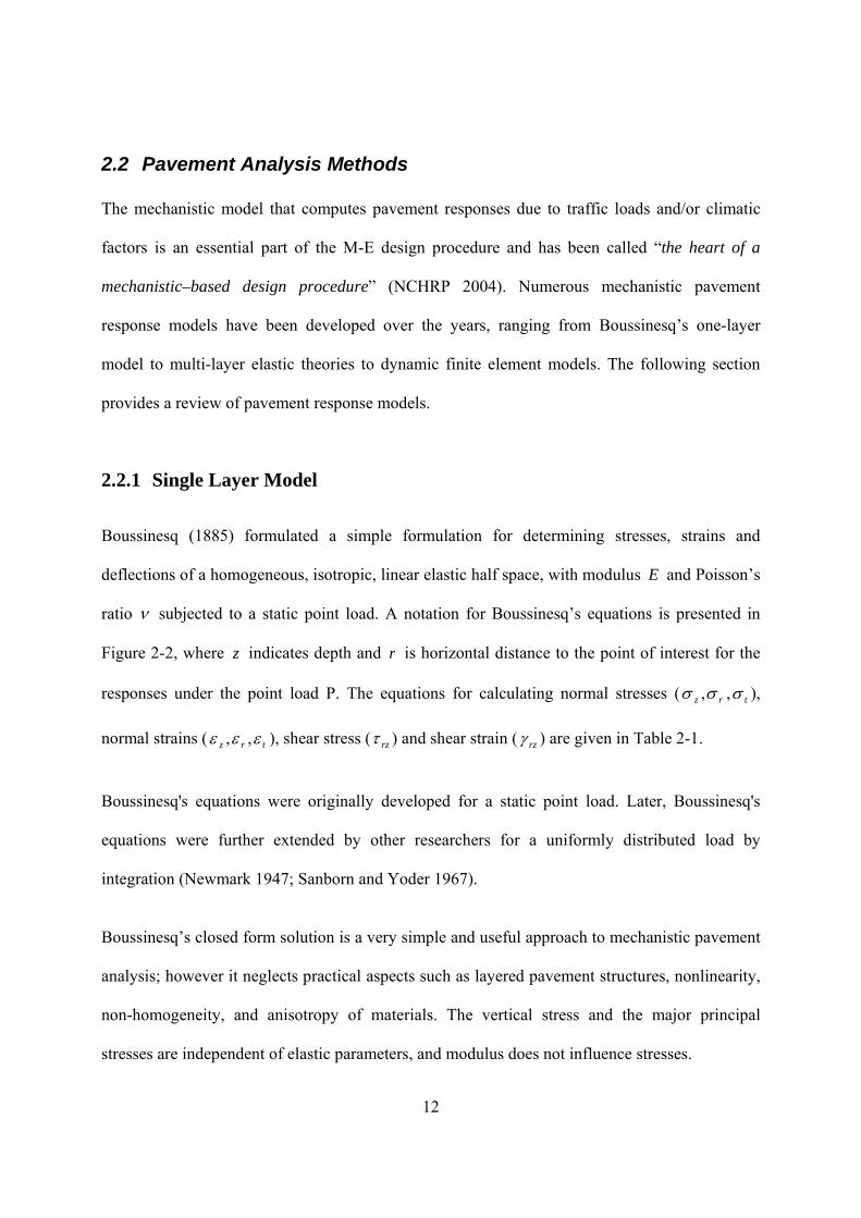
2.2 Pavement Analysis Methods The mechanistic model that computes pavement responses due to traffic loads and/or climatic

factors is an essential part of the M-E design procedure and has been called “the heart of a

mechanistic–based design procedure” (NCHRP 2004). Numerous mechanistic pavement

response models have been developed over the years, ranging from Boussinesq’s one-layer

model to multi-layer elastic theories to dynamic finite element models. The following section

provides a review of pavement response models.

2.2.1 Single Layer Model

Boussinesq (1885) formulated a simple formulation for determining stresses, strains and

deflections of a homogeneous, isotropic, linear elastic half space, with modulus E and Poisson’s

ratio subjected to a static point load. A notation for Boussinesq’s equations is presented in

Figure 2-2, where z indicates depth and r is horizontal distance to the point of interest for the

responses under the point load P. The equations for calculating normal stresses ( rz , , t ),

normal strains ( trz ,, ), shear stress ( rz ) and shear strain ( rz ) are given in Table 2-1.

Boussinesq's equations were originally developed for a static point load. Later, Boussinesq's

equations were further extended by other researchers for a uniformly distributed load by

integration (Newmark 1947; Sanborn and Yoder 1967).

Boussinesq’s closed form solution is a very simple and useful approach to mechanistic pavement

analysis; however it neglects practical aspects such as layered pavement structures, nonlinearity,

non-homogeneity, and anisotropy of materials. The vertical stress and the major principal

stresses are independent of elastic parameters, and modulus does not influence stresses.

13

Figure 2-2: Notation for Boussinesq’s Equation (Tu 2007)

Yoder and Witczak (1975) suggested that Boussinesq theory can be used to estimate subgrade

stresses, strains, and deflections when base and the subgrade have similar stiffness.

14

2.2.2 Layered Elastic Theory

Burmister (1945) developed a solution for two layers and subsequently for a three layers system.

Several layered analytical elastic models have been developed which are generally based on

Burmister (1945).

Acum and Fox (1951) used tabular format to determine normal and radial stresses in three-layer

pavement systems using a circular loading area, two layers thickness, and elastic modulus of the

layers. Schiffman (1962) developed a general solution for determining stresses and

Table 2-1: Boussinesq’s Equations for a Point Load (after Ullidtz 1998)

22

1 23 cos sin

2 1 cosr

P

R

2

(1 2 ) 1cos

2 1 cost

P

R

32

3cos

2z

P

R

32

(1 ) 1 23 cos (3 2 ) cos

2 1 cosr

P

R E

2

(1 ) 1 2cos

2 1 cost

P

R E

32

(1 )3 cos 2 cos

2z

P

R E

22

3cos sin

2rz R

22

(1 )cos sinrz

P

R

15

displacements in a multi-layer elastic system subjected to non-uniform normal surface loads,

tangential surface loads, rigid, semi-rigid, and slightly inclined plate bearing loads. Using

Schiffman’s solution, several computer programs (i.e. WESLEA, VESYS, KENLAYER,

CIRCLY4, BISAR, VEROAD, ELSYM, PDMAP, CHEVRON, JULEA, ILLIPAVE, FENLAP)

have been developed and used in pavement analysis and design to calculate stresses and strains

in multi-layered elastic system (Monismith 2004).

The recently released Mechanistic Empirical Pavement Design Guide (MEPDG) recommends

using the multilayer elastic program JULEA, which is a modified version of WESLEA, and

linear models to compute flexible pavement responses (NCHRP 2004).

Pavement analysis procedures that are derived from the theory of elasticity are based on

simplifications of the real condition. Major simplifications include considering HMA materials

as pure elastic solids and the treatment of vehicular loads as static uniformly distributed circular

area. In most cases, loading situation is dynamic not static. Furthermore, most pavement

materials are neither homogenous nor isotropic, and most have viscoelastic behavior.

Immanuel and Timm (2006) used layered elastic analysis to compare predicted vertical stress in

the base and subgrade layers to field measured vertical pressures obtained from the National

Center for Asphalt Technology (NCAT) Test Track. The authors found that the predicted

pressure was only a reasonable approximation up to vertical pressures of 82 kPa in the base and

48kPa in the subgrade.

Wu et al. (2006) calculated the vertical stress at the bottom of base layer using the multilayer

elastic program ELSYM5 and compared it to data from the Louisiana ALF. The study found the

calculated vertical stresses to be two to eight times higher than the measured field values.

16

2.2.3 Finite Element Analysis

Finite element analysis methods have been developed to model flexible pavement responses.

Raad and Figueroaand (1980) developed ILLIPAVE, a 2-D finite element program, to simulate

flexible pavement behavior. ILLIPAVE uses Mohr-Coulomb failure criterion for subgrade and

non-linear constitutive relationship for pavement materials.

Harichandran et al. (1990) developed a non-linear mechanistic finite element program,

MichPave, for the analysis of flexible pavements. The program was developed for the Michigan

Department of Transportation and is in the public domain. MichPave computes displacements,

stresses, and strains within the pavement due to a single circular wheel load and estimates fatigue

life and rut depth through empirical equations.

Mamlouk and Mikhail (1998) developed a three-dimensional finite element nonlinear dynamic

pavement model to compute dynamic pavement responses. This analysis considered the

viscoelasticity of asphalt and non-linearity of granular and subgrade materials. The model also

considered the truck-pavement interaction resulting from truck speed and dynamic loads

imparted by truck bouncing. The predictions were not validated with field data.

Sargand and Beegle (2002) developed a three-dimensional finite element program, OUPAVE, at

Ohio University to investigate flexible pavement responses subjected to static and dynamic

loadings. Elastic and linear viscoelastic models were used for asphalt material. Calculated

deflections correlated well with falling weight deflectometer (FWD) test data from the Ohio

DEL-23 SHRP Test Road project. Stresses and strains were not investigated as part of this

particular research.

17

Xu et al. (2002) and Park et al. (2005) assessed the condition of pavement layers using FWD

data and the ABAQUS finite element program. This research stressed the importance of

nonlinear behavior of the pavement system to accurately assess pavement deflections.

Hadi and Bodhinayake (2003) used ABAQUS/STANDARD, a three-dimensional finite element

program, to investigate deflection predictions. Asphalt and granular material were considered as

being linear and non-linear respectively. Static and cyclic loads were applied. The best

correlation between field measured and computed deflections was obtained when the materials

were considered non-linear and subjected to cyclic loading.

To characterize granular material using non-linear models, the MEPDG recommends using

DSC2D, a two-dimensional finite element program. The program is recommended for use for

research purposes only (NCHRP 2004).

2.3 Pavement Material Characterization

2.3.1 HMA Material Two major factors are critical in the mechanistic analysis of pavements: (1) the material

characterization method and its accuracy, and (2) the accuracy of mechanistic models to simulate

pavement response (Sousa et al. 1991).

Traditionally, HMA materials have been considered to be purely elastic. However, the behavior

of HMA materials is strongly dependent on temperature and loading frequency. Linear

viscoelastic theory has been successfully used in recent years to describe the behavior of HMA

materials. Elseifi et al. (2006) used finite element models to compare the elastic to linear

18

viscoelastic HMA behavior. The study found that incorporating the viscoelastic constitutive

model improved the accuracy of the model and that elastic theory grossly underestimated the

pavement response.

2.3.1.1 Dynamic Modulus Test HMA is a composite material, whose mechanical behavior is primarily governed by the

viscoelastic nature of the asphalt binder. The fundamental difficulty in the investigation of HMA

viscoelastic property is establishing representative stress-strain relationships. For an unconfined

or confined viscoelastic cylindrical test specimen under a continuous sinusoidal loading, the

stress-strain relationship has been defined using a complex number called the complex modulus

( *E ) (Bari and Witczak 2005; Tran and Hall 2003):

wti

iwt

e

eE

0

0*

( 2-3)

where:

o = Peak stress

o = Peak strain

= Angular velocity

t

= Time

= Phase angle

i

= 1

19

The dynamic modulus is defined as the absolute value of the complex modulus, which is

represented by the ratio of peak stress to peak strain. Due to the nature of viscoelasticity, there is

a time lag between the sinusoidal stress and sinusoidal strain, which is called the phase angle.

2.3.2 Unbound Material Studies have shown that unbound material stress-strain response is non-linear and is a function of

stress condition. Several non-linear constitutive equations have been developed to describe the

stress-strain relation of unbound material as a function of the stress condition. The two most

common models are k and k .

For fine grained materials, the k model is a non-linear relationship that relates the deviatoric

stress ( d ) to resilient modulus ( RM ):

21

kR dM k

( 2-4)

where

RM = Resilient (elastic) modulus

d = Deviatoric stress

21,kk = Constants

The deviatoric stress ( d ) is defined as the difference between major ( 1 ) and minor ( 3 )

principal stress:

1 3d

( 2-5)

20

For coarse grained materials, the k model is a non-linear relationship that relates the bulk

stress to the resilient modulus (MR):

21

kRM k

( 2-6)

where:


= Bulk stress

21,kk = Constants

The bulk stress ( ) is defined as the summation of the principal stresses ( 321 ,, ):

1 2 3 ( 2-7)

Ullidtz (1985) carried out a finite element analysis and suggested a simple non-linear model for

estimating the elastic modulus ( E ):

2

11

k

E kp

( 2-8)

where:

E = Elastic modulus

1 = Major principle stress excluding any static stresses due to the weight of the

material

p = Reference pressure-usually atmospheric (100kPa)

21,kk = Constants

21

Uzan (1985) suggested a nonlinear model for granular soils that considers both deviatoric stress

( d ) and bulk stress( ) :

321

kd

kR kM

( 2-9)

where:


= Bulk stress

d = Deviatoric stress

321 ,, kkk = Constants

2.4 Full-Scale Instrumented Test Facilities Over the past few decades considerable efforts have been made to enhance pavement design and

analysis by measuring direct pavement responses under a variety of loading and environmental

conditions and comparing them to calculated values from response models. Pavement

instrumentation has recently become an important tool in measuring and quantifying pavement

responses and the factors influencing the response parameters. Parameters that are measured in

the field include strain, stress, deflection, moisture, and temperature. Measuring these parameters

in the field also allows for accurate performance model development and mechanistic pavement

analysis.

Several full-scale instrumented test sections have recently been constructed to monitor and

measure in situ pavement response and performance under a variety of loading and

environmental conditions. NCHRP Synthesis 235, published in 1996, indicates that 35 full-scale

22

and accelerated pavement testing facilities exist worldwide, of which 19 have active research

programs (Metcalf 1996). Table 2-2 summarizes the facilities that have been active since 1962

and includes information about the year commissioned, cost of construction, and annual cost

(Hamad 2007). The next section discusses some of the well known instrumented field test

facilities.

2.4.1 Penn State Test Track The Pennsylvania research program, sponsored by the FHWA, undertook a project to evaluate

various pavement instrumentations (Sebaaly et al. 1991). An extensive literature review was

carried out to identify the existing pavement instrumentation and to select the most promising

types of gauges for a field-testing program. The response of selected gauges to dynamic loading

applied by a tractor-semi-trailer at different levels of axle loading, tire pressure, and speed was

investigated using two sections of flexible pavements, 152 and 254 mm HMA layer. The

pavement response data collected in the field-testing program was used to evaluate methods for

back-calculating pavement material properties. It was concluded that the back-calculated moduli

were much more accurate if data from multiple sensors were used in the analysis rather than

from a single sensor.

2.4.2 Minnesota Road (MnRoad) The Minnesota Road Research Project (MnRoad) consists of approximately 40-160m pavement

test sections totaling 9.6km in length. Twenty-three of these test sections have been loaded with

freeway traffic, and the remainder sections have been loaded with calibrated trucks. Electronic

transducers (4572) were embedded in the pavement (Baker et al. 1994). The main purpose of the

23

facility was to verify and improve existing pavement design models, investigate the factors

affecting pavement response, and to develop new pavement models.

Table 2-2:Test Facilities Active since 1962 (Hamad 2007)

2.4.3 Virginia Smart Road

24

The Virginia Smart Road is a 9.6-km connector highway with the first 3.2 km designated as a

controlled test facility. The flexible pavement portion of the Virginia Smart Road includes 12

different flexible pavement designs (Loulizi et al. 2001). Each section is approximately 100m

long. The sections are instrumented with pressure cells, strain gauges, time-domain reflectometry

probes, thermocouples, and frost probes.

2.4.4 Ohio Test Track The Ohio Department of Transportation, in cooperation with the Federal Highway

Administration, constructed a 5-km-long test pavement to encompass four experiments identified

in the Long Term Pavement Performance (LTPP) Specific Pavement Studies (SPS). The test

sections were instrumented with various sensors, and response data were collected under various

axle configurations, loads, speed, and tire types (Sargand et al. 1997). Environmental data was

also collected periodically to investigate the impact of the ground temperature and moisture

content on measured pavement response. The main objective of the Ohio Test Track was to

investigate the interaction of load response to environmental parameters.

2.5 Validation of Response Models with Field Measured Pavement Response

A significant amount of work has been performed in investigating the influence of different load

and environmental factors on pavement response and validating pavement response models.

Chatti et al. (1995) investigated the effects of truck speed and tire pressure on asphalt

longitudinal response. The test section consisted of a 137mm thick surface layer over a 330mm

thick crushed stone base layer and the subgrade was sandy clay. The author found that increasing

25

speed from 2.7 to 64km/hr reduced the asphalt longitudinal strain by approximately 35%. They

also reported that tire pressure did not to have a significant impact on asphalt longitudinal strain

when the speed was 64km/hr. However, when the truck speed decreased the tire pressure impact

increased.

Huhtala et al. (1989) studied the impact of tires and tire pressures on asphalt longitudinal and

transverse strains. Using fatigue performance models, the strain gauge responses showed that

wide-base tires are 2.3 to 4 times more damaging than dual tires.

Huang et al. (2002) performed several numerical analyses with different structural models and

included both static and transient loading. The calculated responses were compared to measured

field values from the Louisiana Accelerated Loading Facility. The study showed that the

predicted response correlated well with field measured pavement responses when the rate-

dependent viscoplastic model for asphalt and elastoplastic models for the other layers were

considered.

Siddharthan et al. (2002) developed a three-dimensional finite element code, 3D-MOVE, that

considered vehicle speed, noncircular contact areas, and the complexity of the contact stress

distributions. Asphalt and unbound materials were characterized as viscoelastic and elastic

material respectively. The dynamic vehicle loading impact was accounted for using a dynamic

load coefficient that is a function of vehicle speed, suspension system, and road roughness. The

applicability of the program was verified using two well-documented full-scale field tests (Penn

State University test track and Minnesota road tests). More than 25 percent deviation was

observed between the predicted and measured strains when the truck was fully loaded. The

26

authors concluded that when the truck was fully loaded, the pavement response was expected to

be significantly affected by the roughness of the road.

Wu and Hussain (2003) performed controlled wheel load tests and FWD tests at the Kansas

Accelerated Testing Laboratory (K-ATL) to investigate pavement response. The authors used

ELSYM5, a multi-layer elastic analysis program, to validate measured pavement responses. The

measured vertical stresses on the top of the subgrade and the tensile strains at the bottom of the

asphalt layer due to FWD loads were found to be very close to those calculated by ELSYM5.

However, measured tensile strains and vertical stresses were higher than those predicted. The

measured tensile strains under the wheel loads were found to increase with increasing number of

wheel load repetitions.

Loulizi et al. (2006) compared measured pavement response with response calculated using

elastic layer analysis performed with four software programs (Kenpave, Bisar 3.0, Elsym5, and

Everstress 5.0) based on the layered elastic theory and two finite element models (ABAQUS and

MichPave). Results indicated that all softwares that were based on elastic layered theory gave the

same response to single and dual tire loading. It was found that the elastic layered theory

underestimates pavement responses at high temperatures and overestimates at low and

intermediate temperatures. As shown in Figure 2-3, at temperatures below 15°C, the measured

asphalt transverse strain at a truck speed of 8km/hr is smaller than the strain calculated using the

elastic layered theory. The measured strain at a truck speed of 8km/hr becomes increasingly

higher than the calculated one at temperatures above 15°C. At temperatures below 28°C, the

measured asphalt transverse strain at a truck speed of 72 km/hr is smaller than the strain

calculated using the elastic layered theory. The measured strain at a truck speed of 72km/hr

27

becomes increasingly higher than the calculated one at temperatures above 28°C. The authors

suggested more research is needed for on layer bonding, anisotropic material properties, and

considering dynamic loading.

Figure 2-3: Measured and Calculated Asphalt Transverse Strain under HMA Layer for

Single Load of 25.8kN (Loulizi et al. (2006))

Elseifi et al. (2006) incorporated a viscoelastic model, which used laboratory determined

parameters, into a finite element model to predict horizontal tensile and vertical shear strains in

the asphalt layers. The comparison of predicted responses with field measured pavement

responses from Virginia Smart Road showed an average prediction error of 15 percent. The

study showed that the calculated pavement responses using elastic models underestimate

pavement response at intermediate and high temperatures.

Fernando et al. (2006) performed an extensive study to investigate the effect of tire contact

stresses on pavement responses. A tire view program was developed by the authors to be used in

28

pavement responses analysis. The authors stated that the relevance of tire contact pressure

distributions decreases as depth increases.

2.6 Environmental Impacts on Pavement Response and Performance It is well known that environmental state play a major role in pavement response and consequent

pavement performance (Salem 2004). The asphalt layer is sensitive to temperature variation and

the unbound materials are sensitive to the moisture content changes. These two environmental

factors, i.e., temperature and moisture content, impact flexible pavement responses and

performance particularly in seasonal frost areas where pavements are susceptible to heave during

winter and then lose their strength during spring thaw (Salem 2004).

Figure 2-4 illustrates the asphalt longitudinal strain for the Alberta Test Road under the standard

axle load of 8165kg in July and October 1976 (Christison et al. 1978).

Figure 2-4: Asphalt Longitudinal Strain versus Vehicle Speed for July and October

1976 (Christison et al. 1978)

29

The average temperature was 17.8oC and 1.7oC during July and October, respectively. The

measured strain was observed to be higher in July, and the difference was more pronounced at

lower speed.

Doré and Duplain (2002) studied the effect of environmental parameters on measured asphalt

longitudinal strain of the St-Célestin test road in Quebec. The test section, 150m long, consisted

of 180mm of asphalt concrete, 300 mm of crushed-rock granular base, 450 mm granular subbase,

and underlying 300 mm layer of silty sand over clay. The pavement sensors included strain

gauges, multi-depth deflectometers, thermistors, moisture sensors, frost gages, piezometers, and

heave gauges. A standard Benkelman beam truck, moving at 50 km/hr, was used to study

pavement response during spring-thaw season, March and April, and recovery period, May. The

authors reported that the strain at the bottom of the asphalt layer increased as the pavement

temperature and the moisture content increased (Figure 2-5).

Solaimanian et al. (2006) measured the tensile strain in Penn State Test Track using various

loading configurations and truck speeds in different seasons. The average tensile strain was

40m/m in February, while 80m/m was observed in September. The air temperature varied

between 15 to 18oC in September and 4 to 5oC in February.

30

Figure 2-5: Asphalt Strain and Pavement Temperature during Spring Thaw (Doré and

Duplain 2002).

31

Chapter 3: Flexible Pavement Response under Dynamic Wheel Loads-A CPATT Full-Scale Instrumented Test Road Study

3 Flexible Pavement Response under Dynamic Wheel Loads-A CPATT Full-Scale Instrumented Test Road Study

32

3.1 Overview In 2000, the Centre for Pavement and Transportation Technology (CPATT) commissioned a two

lane test track in southern Ontario. In 2002, sensors were installed in the test track to monitor

pavement environmental and load-associated responses. The unique CPATT test track facility is

located in a climate with seasonal freeze/thaw events, and is equipped with a remote access data

acquisition system with the capability to sample sensors using a high frequency sampling rate. In

2006, a series of controlled loading tests were performed to investigate pavement dynamic

response due to various loading conditions. The paper describes the CPATT test site, the field

instrumentation program, and the state-of-the-art remote access data acquisition systems. It

describes the 2006 field test program and presents typical sensor data for asphalt strain gauges

and total pressure cells. Field data is then used to determine wheel wander impacts on sensor

readings and temperature effect on measured asphalt longitudinal strains. Testing found that 16

cm wheel wander can reduce asphalt longitudinal strain by 36 percent, and that daily temperature

fluctuations can double the asphalt longitudinal strain.

33

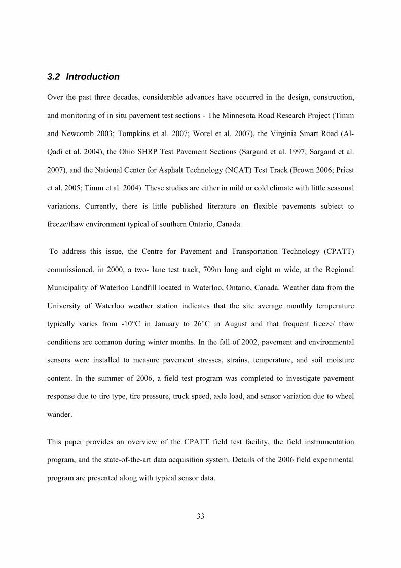
3.2 Introduction Over the past three decades, considerable advances have occurred in the design, construction,

and monitoring of in situ pavement test sections - The Minnesota Road Research Project (Timm

and Newcomb 2003; Tompkins et al. 2007; Worel et al. 2007), the Virginia Smart Road (Al-

Qadi et al. 2004), the Ohio SHRP Test Pavement Sections (Sargand et al. 1997; Sargand et al.

2007), and the National Center for Asphalt Technology (NCAT) Test Track (Brown 2006; Priest

et al. 2005; Timm et al. 2004). These studies are either in mild or cold climate with little seasonal

variations. Currently, there is little published literature on flexible pavements subject to

freeze/thaw environment typical of southern Ontario, Canada.

To address this issue, the Centre for Pavement and Transportation Technology (CPATT)

commissioned, in 2000, a two- lane test track, 709m long and eight m wide, at the Regional

Municipality of Waterloo Landfill located in Waterloo, Ontario, Canada. Weather data from the

University of Waterloo weather station indicates that the site average monthly temperature

typically varies from -10°C in January to 26°C in August and that frequent freeze/ thaw

conditions are common during winter months. In the fall of 2002, pavement and environmental

sensors were installed to measure pavement stresses, strains, temperature, and soil moisture

content. In the summer of 2006, a field test program was completed to investigate pavement

response due to tire type, tire pressure, truck speed, axle load, and sensor variation due to wheel

wander.

This paper provides an overview of the CPATT field test facility, the field instrumentation

program, and the state-of-the-art data acquisition system. Details of the 2006 field experimental

program are presented along with typical sensor data.

34

3.3 CPATT Test Track

3.3.1 Site Information The technological challenges regarding roads and pavements are substantial and include not only

the need for asset preservation but also the provision of adequate levels of service and safety, as

well as, the need for continuing innovation and advancement in all areas. These challenges

formed the basis for a new research initiative in Canada – the University of Waterloo’s Centre

for Pavement and Transportation Technology (CPATT) integrated laboratory and field-tests

facility. Support for the initiative came from a three-way partnership of the public sector

(Federal, Provincial, Regional and Municipal), private sector (contractors, consultants, suppliers,

and manufacturers), and academia.

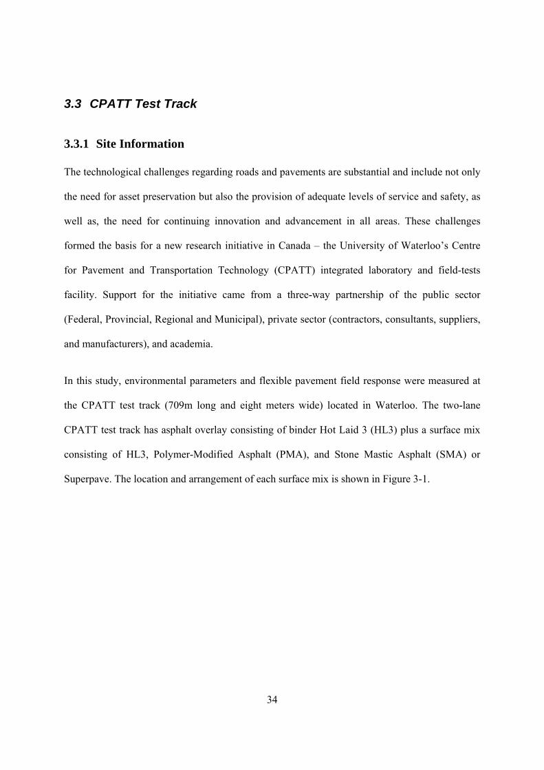
In this study, environmental parameters and flexible pavement field response were measured at

the CPATT test track (709m long and eight meters wide) located in Waterloo. The two-lane

CPATT test track has asphalt overlay consisting of binder Hot Laid 3 (HL3) plus a surface mix

consisting of HL3, Polymer-Modified Asphalt (PMA), and Stone Mastic Asphalt (SMA) or

Superpave. The location and arrangement of each surface mix is shown in Figure 3-1.

35

Figure 3-1: CPATT Test Track Facility Located at Waterloo Region

The instrumented test track section consists of 223 mm and 185 mm of HL3 on the west and east

lane respectively. The HL3 mix consists of 40 percent crushed gravel, 45% asphalt sand, 15%

screenings, and 5.3% PG 58-28 asphalt cement. Below the HL3 are 200mm of Granular A base

aggregate and 300mm of Granular B subbase aggregate. Compacted Granular A, 900mm in

depth, is located below the subbase aggregate. Below the compacted Granular A is site subgrade

that consists of compacted fill and well compacted clayey silt with some gravel. Granular A, as

defined in Ontario Provincial Standard Specification (OPSS) 1010, consists of crushed rock

composed of hard, uncoated, fractured fragments reduced from rock formations or boulders of

uniform quality while Granular B consists of clean, hard, durable uncoated particles from

deposits of gravel or sand (MTO 2003). Further details on the test track facility including its

construction and pavement performance can be found in Knight et al. (2004) and Tighe et al.

(2003).

36

3.3.2 Field Monitoring Program A state-of-the-art field instrumentation and data acquisition program was developed as part of

the CPATT field monitoring program. Sensors were installed to measure asphalt and soil strain,

vertical stress, soil moisture content, and ground temperature. Figure 3-2 shows sensor

distribution (ASG is asphaltic strain gauge, TPC is total pressure cell, T is thermistors, and TDR

is Time Domain Reflectometer). The following sections, adopted from Adedapo (2007), provide

details on the pavement load and environmental sensors and the state-of-the-art data acquisition

system.

Figure 3-2: Instrumented Section Profile and Sensor Distribution Layout

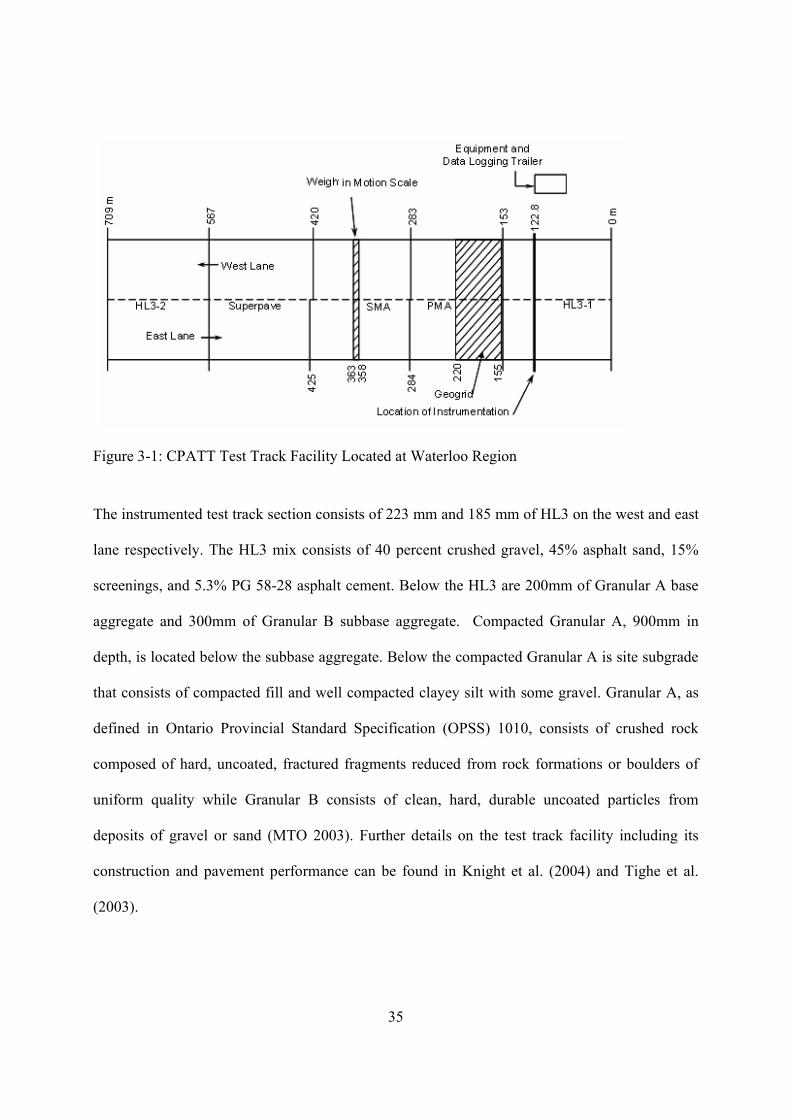
3.3.2.1 Load Sensors Asphalt Strain Gauges (ASG)

To measure asphalt longitudinal strains at the base of the asphalt layer, five ASG-152 H-type

asphalt strain gauges, manufactured by Construction Technology Laboratories (CTL) Group Inc.

were installed. These gauges were chosen due to their reliability, durability, low cost, short

37

delivery time, and excellent performance at other test sites. Prior to installation, calibration and

functionality of each gauge was checked in the laboratory. Figure 3-2 shows the location of the

five asphalt strain gauges (ASG1 to ASG5). ASG3 was placed at the road centerline, while

ASG1 and ASG2 were placed 690mm and 2700 mm from the west pavement edge respectively.

ASG5 and ASG4 were placed 1380mm and 3200mm from the east pavement edge respectively.

To ensure that the asphalt strain gauges were bounded to the asphalt base course, all asphalt

strain gauges were placed in a sand-asphalt binder mixture consisting of sand and PG 64-22

binder (Figure 3-3).

Figure 3-3: H-type Asphalt Strain Gauge Prior to Placement of HL3 Asphalt (Adedapo

2007)

Earth Pressure Cells (TPC)

To record changes in vertical stress during construction and vertical stress due to dynamic wheel

loads, Campbell Scientific RST pressure cells were installed (RST TP -12-S, TP-9-S, and TP-6-S

pressure cells with 172kPa, 345kPa and 690kPa stress capacity). Pressure cells were selected due

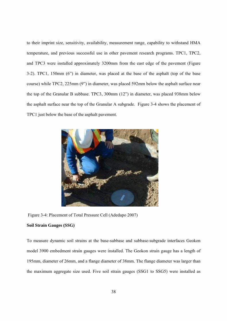
38

to their imprint size, sensitivity, availability, measurement range, capability to withstand HMA

temperature, and previous successful use in other pavement research programs. TPC1, TPC2,

and TPC3 were installed approximately 3200mm from the east edge of the pavement (Figure

3-2). TPC1, 150mm (6”) in diameter, was placed at the base of the asphalt (top of the base

course) while TPC2, 225mm (9”) in diameter, was placed 592mm below the asphalt surface near

the top of the Granular B subbase. TPC3, 300mm (12”) in diameter, was placed 938mm below

the asphalt surface near the top of the Granular A subgrade. Figure 3-4 shows the placement of

TPC1 just below the base of the asphalt pavement.

Figure 3-4: Placement of Total Pressure Cell (Adedapo 2007) Soil Strain Gauges (SSG)

To measure dynamic soil strains at the base-subbase and subbase-subgrade interfaces Geokon

model 3900 embedment strain gauges were installed. The Geokon strain gauge has a length of

195mm, diameter of 26mm, and a flange diameter of 38mm. The flange diameter was larger than

the maximum aggregate size used. Five soil strain gauges (SSG1 to SSG5) were installed as

39

shown in Figure 3-2. Soil strain gauges SSG1 and SSG2 were installed approximately 990mm

from the west pavement edge and 601 and 969mm respectively below the asphalt surface. Soil

strain gauges SSG4 and SSG5 were installed approximately 1350mm from the east pavement

edge and 580 and 901mm below the base of the asphalt respectively. Gauge SSG3 was installed

at the base of the asphalt (top of the base course) below the road centerline.

3.3.2.2 Environmental Sensors Time-Domain Reflectometer Probes (TDR)

To measure base and subbase daily and seasonal water content changes, two Campbell Scientific

CS616 TDR probes (TDR1 and TDR2) were installed 800 and 1150mm below the west lane

asphalt surface respectively. The TDR probes were selected due to their performance,

survivability, cost, and ability to integrate with available existing data acquisition loggers. The

TDR probes consisted of two parallel conducting rods 300mm in length with a separation

distance of 32mm. All sensors were calibrated prior to installation using site Granular A and B

aggregates.

Thermistor Probes (T)

To measure daily and seasonal temperature changes in pavement structure, four Campbell

Scientific T107B thermistors (T1 to T4) were installed 223, 530, 1134, and 1734mm below the

west lane asphalt surface respectively. Campbell Scientific reports the thermistors precision to be

0.1 °C.

40

3.3.3 Data Acquisition A Campbell Scientific CRX10 data logger was used to monitor the thermistors and the TDR

probes using a sampling rate of 0.0033Hz (1 reading every 5 minutes). This sampling rate was

deemed sufficient to record daily sensor changes. All other sensor data was collected using

Somat eDAQ-plus®, a data logger with the sampling rate set at 0.01Hz (1 reading every 1.67

minutes) in idle mode and 1500Hz when triggered by a traffic load. The high sampling rate was

used to capture the millisecond truck load moving over the sensors while the low sampling rate

was used to record sensor changes due to environmental factors. The CPATT test track is one of

the few instrumented test tracks that has the ability to collect sensor data at a high sampling rate.

The Somat eDAQ system is a compact, rugged, and modular data acquisition system capable of

collecting a wide range of signal types directly from sensors - strain, analog to ±80V, digital,

frequency, and temperature. The eDAQ unit used for this research has the following modules:

processor, high-level simultaneous sampling board, and high level board. The processor speed is

266MHz with integrated floating point and 256MB on board DRAM is available for the

operating system. The speed of the master sample clock is 100kHz and it has a 2GB memory

capacity for onboard data storage. The PC-to-eDAQ communication is via Ethernet 100BaseT

and RS232 serial communication. Test Control software (TCE), a Windows TM based software

application, was used to set up and define test requirements in the eDAQ. TCE software was

used to: create the test setup files that define and calibrate transducer channels; define data

modes and computed channels for online data calculations and analyses; specify triggering

conditions for collection of sensor data; monitor sensors using run-time displays; and initialize,

start, stop, and upload sensor stored data.

41

3.3.4 Power Supply and Management

For long-term field monitoring in remote locations, power supply and management plays a

critical role for the operation and collection of sensor data. For this project, power was supplied

using two 12V deep cycle batteries that were recharged using a solar panel (Figure 3-5).

To conserve battery power during the winter - when the duration of solar recharge was limited -

a programmable timer was used to automatically turn the system off and on at predefined times.

This power system was found to work well, to be robust, and a cost- effective method to power

the sensors and the eDAQ data acquisition system.

Figure 3-5: Solar Panel for Recharging Batteries at Test Site (Adedapo 2007)

42

3.3.5 Remote Monitoring System A unique remote monitoring system was developed so that the eDAQ field computer could be

monitored and the sensor data could be downloaded using a secure internet connection. Figure

3-6 shows the secure remote monitoring system. The remote monitoring system allowed for daily

data upload and the ability to check sensor functionality without the need for site visit. During

one data check, several asphalt strain gauges were found not to be working. A site visit revealed

that sensor wires had been accidentally cut during grass mowing. All wires were promptly fixed

resulting in only a short period with limited data collection.


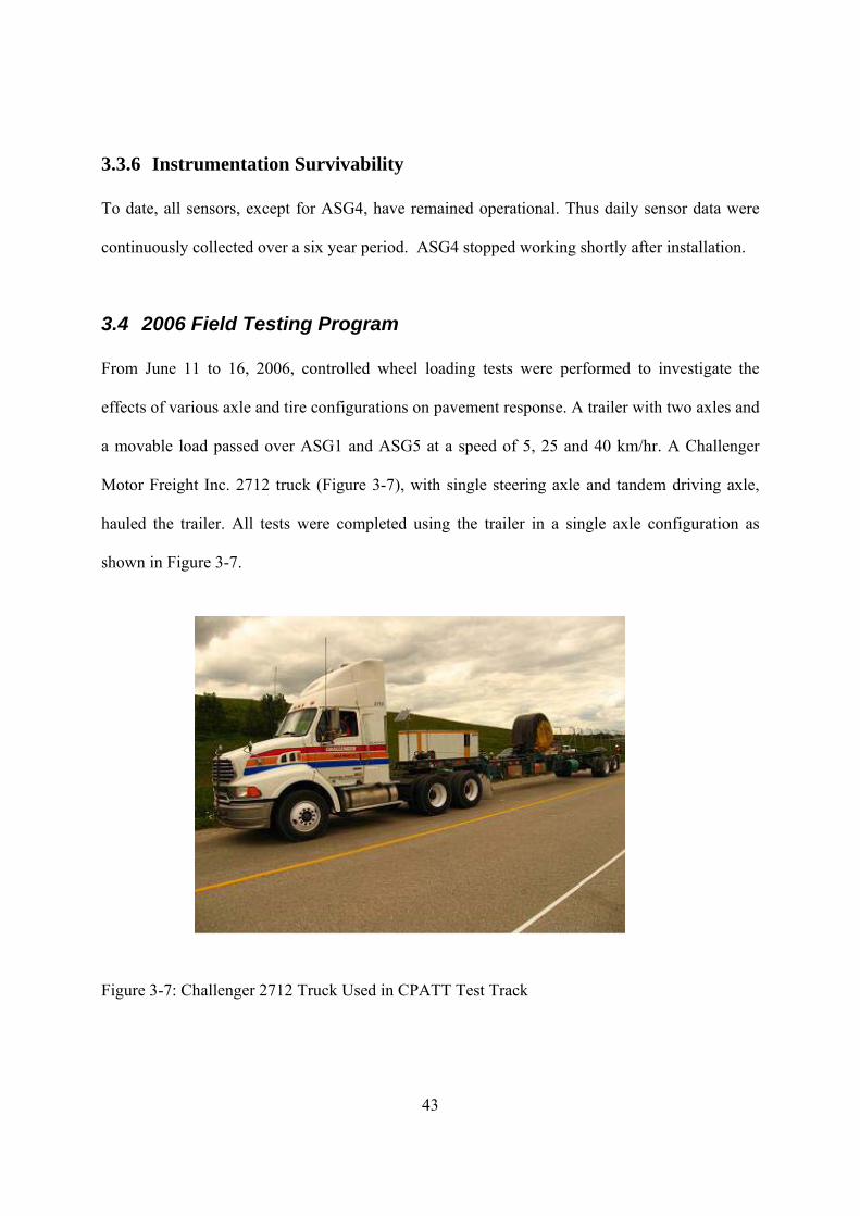
43

3.3.6 Instrumentation Survivability

To date, all sensors, except for ASG4, have remained operational. Thus daily sensor data were

continuously collected over a six year period. ASG4 stopped working shortly after installation.

3.4 2006 Field Testing Program From June 11 to 16, 2006, controlled wheel loading tests were performed to investigate the

effects of various axle and tire configurations on pavement response. A trailer with two axles and

a movable load passed over ASG1 and ASG5 at a speed of 5, 25 and 40 km/hr. A Challenger

Motor Freight Inc. 2712 truck (Figure 3-7), with single steering axle and tandem driving axle,

hauled the trailer. All tests were completed using the trailer in a single axle configuration as

shown in Figure 3-7.

Figure 3-7: Challenger 2712 Truck Used in CPATT Test Track

44

The trailer was configured so that a single axle load could be quickly changed to prescribed

values between 7,000 to 15,000kg. All axle loads were set using a mobile scale placed under

each axle tire as shown in Figure 3-8. Tests were completed using six tire types: 11R22.5,

275/80R22.5, 295/75R22.5, and 285/70R22.5 dual tires, and 455/55R22.5 and 445/50R22.5

wide-base tires. Tire inflation pressures ranged from 482 to 827kPa.

Figure 3-8: Mobile Scale Used to Verify Single Axle Loads

Multiple passes of the trailer were conducted for each load configuration to ensure that at least

three wheel loads passed over the sensors within a prescribed offset limit (50 mm). Video

cameras along with pavement markings (Figure 3-9) were used to verify when a wheel passed

within the prescribed limit.

For each axle load and tire configuration the tire contact area was measured by obtaining a static

tire imprint. Pressure-sensing pads were also used to determine the tire static contact pressure

(Figure 3-10).

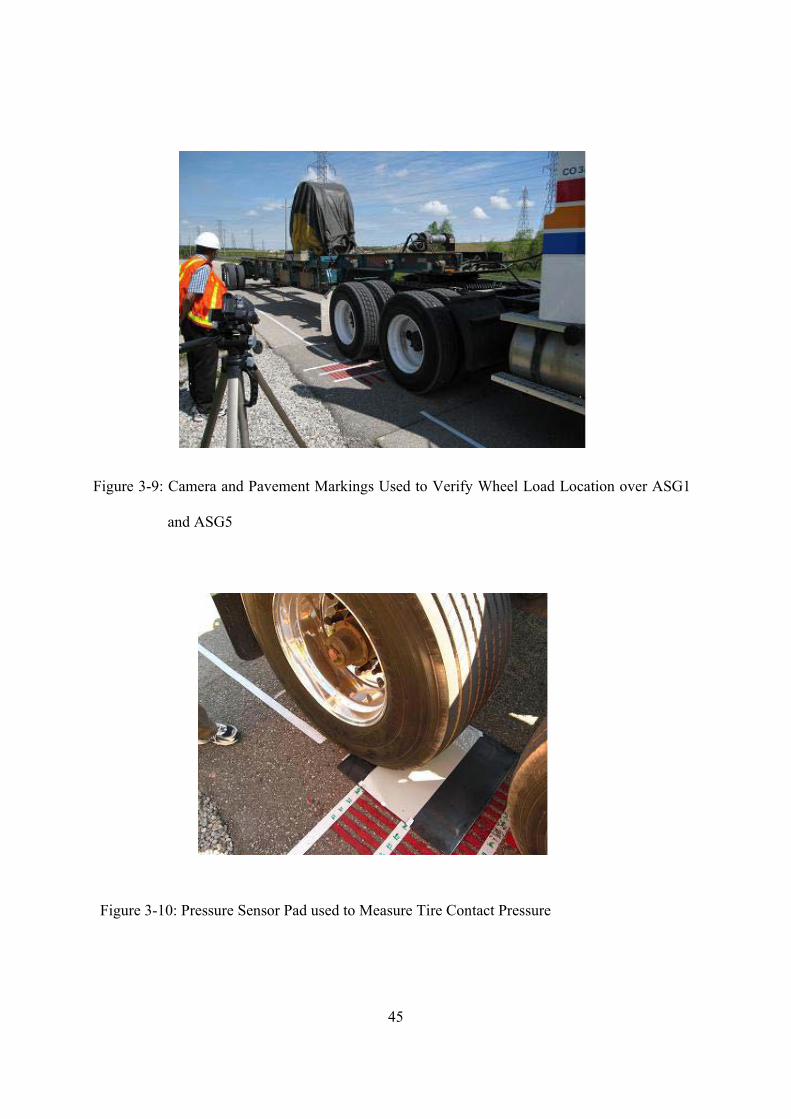
45

Figure 3-9: Camera and Pavement Markings Used to Verify Wheel Load Location over ASG1

and ASG5

Figure 3-10: Pressure Sensor Pad used to Measure Tire Contact Pressure

46

3.5 Data Collection and Analysis Pavement sensor data was collected at a rate of 1500Hz for each wheel pass. Test Control

software (TCE) was used to set up test requirements in eDAQ data acquisition system and to

specify triggering conditions for collection of test data. The recorded high speed signals were

processed using Infield Somat field analysis software program that is optimized for use with

Somat hardware. This software allowed for quick analysis of the large data files. Typical asphalt

longitudinal strain gauge and total pressure cell data are shown in Figure 3-11 and Figure 3-12

respectively.

Figure 3-11: Asphalt Strain Gauge (ASG5) Response during the Passing of the Truck and

Trailer Wheel Loads

47

Figure 3-11 shows ASG5 asphalt longitudinal strain measured at the bottom of asphalt pavement

layer under a wheel load of 49kN moving at a speed of 25km/hr. The first pulse, at 1 second,

represents the passing of the truck steering axle over the strain gauge. The following two pulses,

at approximately 1.4 and 1.6 seconds, are the truck’s dual tandem drive wheels passing over the

strain gauge. The third pulse, at approximately 3.2 seconds, represents the passing of the

prescribed trailer wheel load. All wheel passes show the following characteristic behavior –

asphalt compression followed by asphalt tension then a second compression wave. Following

each truck and trailer pass, the strain gauge was observed to quickly return to its preloading

strain values (approx. 1000 m/m). Sebaaly and Mamlook (1987), Al-Qadi et al. (2004),

Immanuel and Timm (2006), and Stoffels et al. (2006) reported similar asphalt longitudinal

Figure 3-12: Total Pressure Cell (TPC1) Response during the Passing of the Truck and Trailer

Wheel Loads

48

strain gauge responses. Figure 3-12 shows TPC1 vertical stress when the truck and trailer with a

49kN wheel load passed over ASG5 at a speed of 25km/hr. The first peak pressure response, at

approximately 1 second, represents the passing of the steering axle while the two following

pressure peaks represent the passing of the truck dual tandem drive wheels. The third pressure

peak, at approximately 3.3 seconds, represents the passing of the prescribed trailer wheel load.

Sebaaly and Mamlook (1987), Al-Qadi et al. (2004), Immanuel and Timm (2006), Loulizi et al.

(2001), and Priest et al. (2005) reported similar total pressure cell responses.

Temperature and soil moisture content data were recorded at five minute intervals throughout the

week of testing. Figure 3-13 shows changes in thermistor probes T-1, T-2, T-3, and T-4 during

the week. Temperature data from all probes show a sinusoidal distribution with decreasing

magnitude as the probe depth below the asphalt surface increases. It also shows that T-1

minimum and maximum daily temperature increased each day and that the daily temperature

variation ranged from 5 to 7.8ºC. Daily air temperatures were found to range from a low of 15ºC

to a high of 35ºC with the nightly low and afternoon high increasing throughout the week.

Asphalt surface temperatures were also recorded for every run using a heat sensor gun. Soil

moisture content was recorded to be 13 and 21 percent at TDR1 and TDR2 respectively during

the week of testing.

The following section presents a partial analysis of the field data collected to determine the

impact of wheel wander and daily temperature changes on asphalt strain gauge readings during

the passing of a constant wheel load.

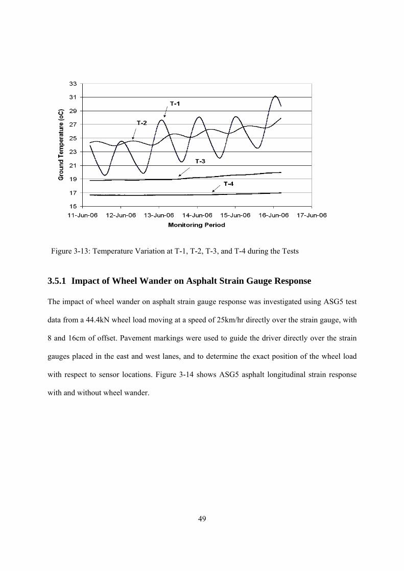
49

3.5.1 Impact of Wheel Wander on Asphalt Strain Gauge Response The impact of wheel wander on asphalt strain gauge response was investigated using ASG5 test

data from a 44.4kN wheel load moving at a speed of 25km/hr directly over the strain gauge, with

8 and 16cm of offset. Pavement markings were used to guide the driver directly over the strain

gauges placed in the east and west lanes, and to determine the exact position of the wheel load

with respect to sensor locations. Figure 3-14 shows ASG5 asphalt longitudinal strain response

with and without wheel wander.

Figure 3-13: Temperature Variation at T-1, T-2, T-3, and T-4 during the Tests

50

Figure 3-14 shows that when the wheel load passes directly over the strain gauge it results in

500m/m of asphalt longitudinal strain, while 8 and 16cm of wheel wander results in 420 and

330m/m respectively. Thus, 16cm of wheel wander reduces the measured asphalt longitudinal

strain by 36 percent. Figure 3-14 also shows that the compression part of the wave is not very

sensitive to wheel wander.

Figure 3-15 and Figure 3-16 show west and east lanes wheel wander distributions for 270 wheel

passes. In these figures, positive offset means that the wheel passed towards the edge of the

pavement, and negative offset means that the wheel passed towards the road centerline. The

distributions show that -25 to 20cm of wheel wander occurred in the west lane while -20 to 30cm

occurred in the east lane. The asymmetrical shape of distributions indicates that the driver had a

bias towards the road centerline when travelling in the west lane and towards the road shoulder

when travelling in the east lane.

Figure 3-14: ASG5 Strain Response under Different Wheel Lateral Offset

51

3.5.2 Effect of Temperature on Measured Longitudinal Strains To determine the impact of temperature changes on the measured asphalt longitudinal strain with

a constant wheel load, test data from the following test configuration was used - dual tires

Figure 3-15: Lateral Offset Distribution of the Runs - West Lane

Figure 3-16: Lateral Offset Distribution of the Runs - East Lane

52

(11R22.5D) with a tire inflation pressure of 689kPa, an axle load of 49kN moving directly over

(no wheel wander) the sensors at a speed of 25km/hr. Figure 3-17 shows ASG5 and ASG1

asphalt longitudinal strain variation with asphalt mid-depth temperature. The asphalt mid-depth

temperature was determined by averaging the heat gun measured asphalt surface temperature and

the temperature measured at base of the asphalt layer (T-1). Figure 3-17 shows that ASG5

asphalt longitudinal strain doubled from 250m/m at 20.5ºC to 500m/m at 34ºC while ASG1

almost doubled from 185m/m at 20.5ºC to 390m/m at 34ºC. Both strain gauges indicate that

asphalt longitudinal strain is sensitive to small changes in asphalt mid-depth temperature. It

should be noted that ASG1 consistently had lower strain than ASG5. This lower measured strain

is inferred to be the result of the thickness of the west lane asphalt being 38mm more than the

east lane. Analysis of the field data showed that exponential relationships, with R2 of greater than

0.9, exist between asphalt longitudinal strain and mid-depth temperature. Al-Qadi et al. (2002),

Loulizi et al. (2002), Priest et al. (2005), and Stoffels et al. (2006) also reported exponential

relationships between measured asphalt longitudinal strain and asphalt temperature.

53

3.6 Summary and Conclusions An overview of the CPATT test track, field instrumentation, and the state-of-the-art data

acquisition system is presented. This unique facility, located in a climate with seasonal

freeze/thaw events, is equipped with an internet accessible data acquisition system capable of

reading and recording sensors using a high sampling rate (1500 Hz). Field data was analyzed to

determine the effects of wheel wander and changes in asphalt temperature on sensor readings.

Main conclusions drawn from this study are:

The CPATT instrumentation system has worked exceptionally well for over six years

with a survivability rate of approximately 95%.


y = 95.452e0.048x

R2 = 0.9115

y = 67.562e0.051x

R2 = 0.9075

150

200

250

300

350

400

450

500

20 22 24 26 28 30 32 34

Asphalt Mid-Depth Temperature (oC)

Lo

ng

itu

din

al A

sph

alt

Str

ain

(

mm

)

ASG1

ASG5

54

Two data acquisition systems were implemented – low frequency to record daily

temperature and soil moisture content changes and high frequency to record pavement

stresses and strains due to passing wheel loads.

The remote monitoring system considerably reduced the required site visits and resulted

in ensuring that continuous data collection occurred with limited site visits.

Longitudinal strain response shows that the pavement fully recovers after each truck and

trailer wheel pass.

16 cm of wheel wander reduced measured pavement strains by 36 percent.

An exponential relationship was found between asphalt longitudinal strains and asphalt

mid-depth temperature.

3.7 Acknowledgment The authors would like to thank the Natural Science and Engineering Research Council of

Canada (NSERC) and CPATT for providing research funding. We would also like to

acknowledge the Ministry of Transportation Ontario (MTO), Challenger Motor Freight Inc., and

Michelin Canada for their help in organizing and developing the 2006 field test program.

55

Chapter 4: Validation of Hot-Mix Asphalt Dynamic Modulus using Field Measured Pavement Response

4 alidation of Hot-Mix Asphalt Dynamic Modulus using Field Measured Pavement Response

56

4.1 Overview The current Mechanistic–Empirical Pavement Design Guide (MEPDG) proposes using the

laboratory dynamic modulus test to determine the time-temperature dependent properties of Hot

Mix Asphalt (HMA) materials. To date, limited measurements have been performed to compare

the HMA behavior of laboratory dynamic modulus test with the field measured pavement

response. The objective of this study was to compare and validate laboratory determined HMA

dynamic modulus with the results of field measured asphalt longitudinal strains. Under constant

loading frequency, the laboratory determined dynamic modulus for Hot Laid 3 (HL3) was found

to decrease exponentially when the temperature of the asphalt mix increased. Controlled wheel

load experiments, performed using a constant truck speed, found that HL3 asphalt longitudinal

strain increased exponentially with an increase in asphalt mid-depth temperature. The

comparison of both exponential relationships showed that the laboratory determined dynamic

modulus was inversely proportional to the field measured asphalt longitudinal strain.

57

4.2 Introduction The current Mechanistic–Empirical Pavement Design Guide (MEPDG), introduced by the

recently completed NCHRP Project 1-37A and currently under evaluation by transportation

agencies, proposes the use of the time-temperature dependant complex modulus ( *E ) of HMA

(NCHRP 2004). Dynamic modulus test is also being used as a Simple Performance Test to

predict rutting and fatigue cracking in HMA (NCHRP 2004).

The use of complex modulus ( *E ) in the design guide has several advantages over stiffness

parameters such as resilient modulus ( RM ). Loulizi et al. (2006) compared laboratory dynamic

modulus and resilient modulus test data for HMA. In this study, resilient and dynamic modulus

tests were performed at five temperatures on two typical mixes used in the Commonwealth of

Virginia and the test results compared. The dynamic modulus was determined using six

frequencies and the resilient modulus test was determined at one loading frequency. The authors

found a strong relationship between the dynamic modulus test performed at 5Hz and the resilient

modulus. The authors concluded that the dynamic modulus test provides a better characterization

of HMA than the resilient modulus test due to its full characterization of the mix over a range of

temperatures and loading frequencies.

To date, limited measurements have been performed to compare the HMA behavior of laboratory

dynamic modulus test with the field measured pavement response. This paper describes a series

of laboratory dynamic modulus test performed on Hot Laid 3 (HL3) asphalt mix used at the

Centre for Pavement and Transportation Technology (CPATT) test track. It also discusses field

controlled wheel load experiments performed at the CPATT test track facility, and presents

typical HL3 pavement response. An analytical approach is then proposed to validate laboratory

58

measured dynamic modulus with the result of field wheel load experiments. Conclusions and

recommendations are then presented.

4.3 Dynamic Modulus Test Uzarowsky (2006) presents the results of dynamic modulus tests performed on several mixes

including HL3 - the mix used in the instrumented section of CPATT test track. The HL3 mix was

designed using the Marshall methodology to meet requirements of Ontario Provincial Standard

Specification (OPSS) 1150 (MTO 2003). The HL3 mix consisted of 40 percent crushed gravel,

45% asphalt sand, 15% screenings, and 5.3% PG 58-28 asphalt cement. HL3 specimens, 150mm

in diameter, were prepared in accordance with AASHTO TP62-03 standard (AASHTO 2003)

using a Superpave Gyratory Compactor. Dynamic modulus test specimens, 100 mm in diameter,

were then cored from the 150mm specimens and the average air void was determined to be 6.2

percent. An Interlaken UniTest Control System with pre-programmed software was then used to

determine the dynamic modulus of HL3 at five testing temperatures (-10, 4.4, 21.1, 37.8, and

54.4 oC) and at six loading frequencies (0.1, 0.5, 1.0, 5.0, 10.0, and 25.0 Hz). AASHTO (2003)

procedures were used to determine the dynamic modulus ( *E ) over the last five loading cycles

using Equation 4-1:

o

oE

* ( 4-1)

where:

o =Average peak stress

o = Average peak strain

59

HL3 dynamic modulus test results, reported by Uzarowsky (2006), are summarized in Table 4-1.

Table 4-1: HL3 Dynamic Modulus

Dynamic Modulus (MPa) Loading Frequency

(Hz) -10oC 4.4 oC 21.1 oC 37.8 oC 54.4 oC

25 29035.6 18234.1 8517.0 3677.7 1771.9

10 26140.9 15782.4 6724.6 2531.6 1241.3

5 23758.5 14155.5 5632.2 2001.5 1062.6

1 19463.9 8970.2 3567.4 1324.5 789.3

0.5 17024.6 8410.7 2903.3 1139.1 723.1

0.1 12462.5 5904.9 1923.6 876.3 543.0

4.3.1 Changes in Dynamic Modulus with Temperature

Figure 4-1 shows the dynamic modulus with respect to temperature for each loading frequency.

This figure shows that for each loading frequency, the dynamic modulus decreases exponentially

with increasing temperature. Using the least squared regression method, Equation 4-2, an

exponential relationship, was found to fit the test data with a 2R of 0.99:

for

( 4-2)

where:

)(* TE = Dynamic modulus as a function of temperature (MPa)

f

= Test loading frequency (Hz)

of = Constant loading frequency (Hz)

TbeaTE )(*off

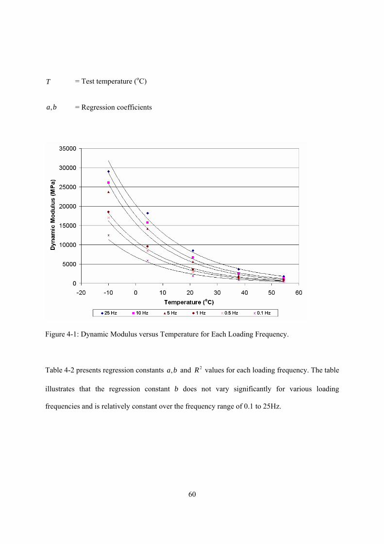
60

T

= Test temperature (oC)

ba,

= Regression coefficients

Figure 4-1: Dynamic Modulus versus Temperature for Each Loading Frequency.

Table 4-2 presents regression constants ba, and 2R values for each loading frequency. The table

illustrates that the regression constant b does not vary significantly for various loading

frequencies and is relatively constant over the frequency range of 0.1 to 25Hz.

61

4.3.2 Changes in Dynamic Modulus with Frequency Dynamic modulus versus frequency for each testing temperature is shown in Figure 4-2. This

figure shows that for each testing temperature the dynamic modulus increases non-linearly when

the frequency increases. Using the least squared regression method, Equation 4-3, a non-linear

relationship, was found to fit the test data with a R2 of 0.97 to 0.99:

dfcfE .)(*

for

( 4-3)

where:

)(* fE

= Dynamic modulus as a function of frequency (MPa)

T

= Test temperature (oC)

oT = Constant test temperature (oC)

Table 4-2: ba, and 2R Values for Each Loading Frequency

Loading Frequency a b R2

25 20,381 -0.045 0.99

10 17,615 -0.049 0.99

5 15,594 -0.050 0.99

1 11,028 -0.050 0.99

0.5 9,688 -0.051 0.99

0.1 6,862 -0.050 0.98

oTT

62

f = Test loading frequency (Hz)

dc,


Figure 4-2: Dynamic Modulus versus Frequency for Each Testing Temperature

Table 4-3 presents regression coefficients c, d and R2 values for each testing temperature. This

table shows that the d value for all testing temperatures varied from 0.151 to 0.273 over the

temperature range of -10 to 54.4 oC, while the d value is relatively constant over the same range.

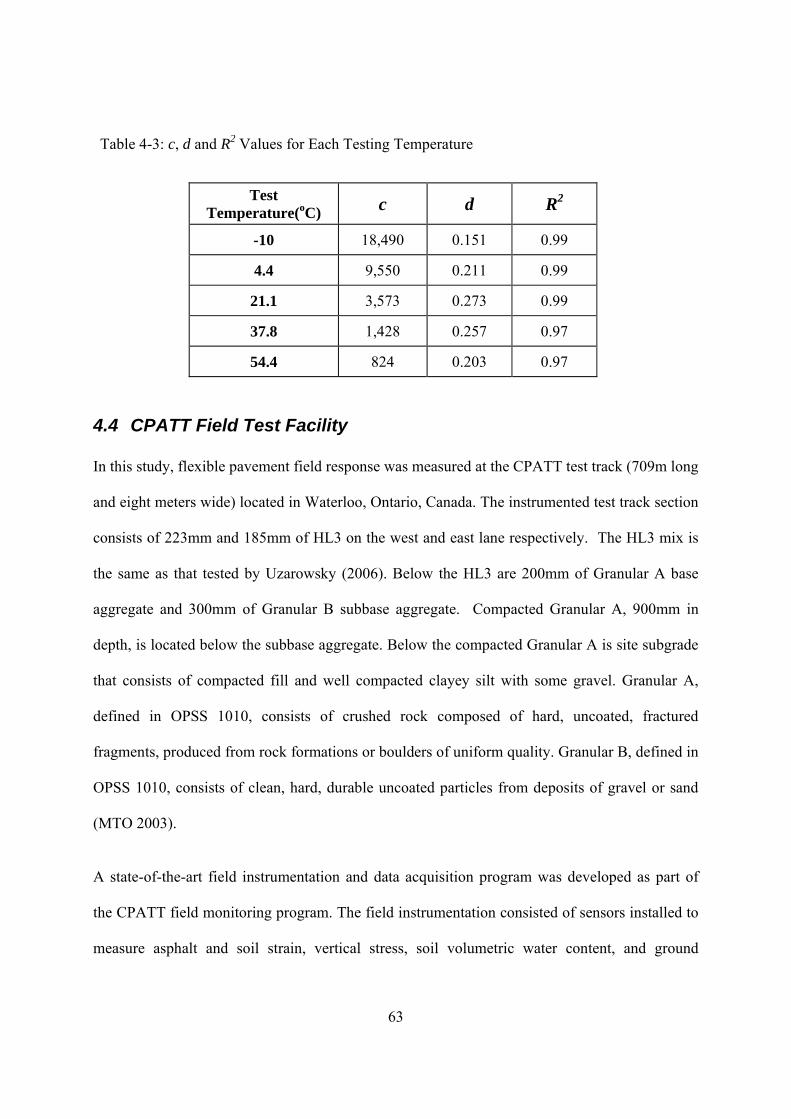
63

4.4 CPATT Field Test Facility In this study, flexible pavement field response was measured at the CPATT test track (709m long

and eight meters wide) located in Waterloo, Ontario, Canada. The instrumented test track section

consists of 223mm and 185mm of HL3 on the west and east lane respectively. The HL3 mix is

the same as that tested by Uzarowsky (2006). Below the HL3 are 200mm of Granular A base



that consists of compacted fill and well compacted clayey silt with some gravel. Granular A,

defined in OPSS 1010, consists of crushed rock composed of hard, uncoated, fractured

fragments, produced from rock formations or boulders of uniform quality. Granular B, defined in

OPSS 1010, consists of clean, hard, durable uncoated particles from deposits of gravel or sand

(MTO 2003).

A state-of-the-art field instrumentation and data acquisition program was developed as part of

the CPATT field monitoring program. The field instrumentation consisted of sensors installed to

measure asphalt and soil strain, vertical stress, soil volumetric water content, and ground

Table 4-3: c, d and R2 Values for Each Testing Temperature

Test Temperature(oC) c d R2

-10 18,490 0.151 0.99

4.4 9,550 0.211 0.99

21.1 3,573 0.273 0.99

37.8 1,428 0.257 0.97

54.4 824 0.203 0.97

64

temperature. Figure 4-3 shows the instrumented section profile and sensor distribution layout

(ASG is asphaltic strain gauge, TPC is total pressure cell, T is thermistors, and TDR is Time

Domain Reflectometer).

Figure 4-3 : Instrumented Section Profile and Sensor Distribution Layout

All load sensor data was collected using a Somat eDAQ-plus®, data logger with the sampling

rate set at 0.01 Hz (1 reading every 1.67 minutes) in idle mode and 1500 Hz when triggered by a

traffic load. The high sampling rate was used to capture the millisecond truck load moving over

the sensors while the low sampling rate was used to record sensor changes due to environmental

changes. The CPATT test track is one of the few instrumented test tracks that has the ability to

collect sensor data at a high sampling rate. Tighe et al. (2003) report details on the CPATT test

track facility construction and pavement performance.

4.5 Field Testing Program A series of controlled wheel loading tests was carried out on the instrumented CPATT test track

section with the objective of quantifying the pavement response to truck loading under different

65

wheel load configurations and varying daily temperature. A Challenger Motor Freight Inc. 2712

truck, with a single steering axle and a tandem driving axle was used to haul a trailer in a single

axle configuration so that the outer trailer tire passed over ASG1 and ASG5 at a speed of 5, 25

and 40km/hr. Multiple passes of the truck were conducted for each load configuration to ensure

that at least three wheel loads passed directly over the sensors. Video cameras along with

pavement markings were used to verify when a wheel passed directly over each strain gauge.

The vertical stress and asphalt longitudinal strains were measured and recorded at a frequency of

1500Hz. Figure 4-4 shows measured ASG5 longitudinal strain at the bottom of asphalt layer

under a wheel load of 49kN moving at a speed of 25km/hr. The first strain pulse, at 1 second,

represents the passing of the truck steering axle over the strain gauge. The following two strain

pulses, at approximately 1.4 and 1.6 seconds, are the truck’s dual tandem drive wheels passing

over the strain gauge. The third pulse, at approximately 3.2 seconds, represents the passing of the

prescribed trailer wheel load. Figure 4-5 shows TPC1 vertical stress when the truck and trailer

with a 49kN wheel load passed directly over ASG5 at a speed of 25km/hr. The first peak

pressure response, at approximately 1 second, represents the passing of the steering axle while

the two following pressure peaks represent the passing of the truck dual tandem drive wheels.

The third pressure peak, at approximately 3.3 seconds, represents the passing of the prescribed

trailer wheel load.

66

4.5.1 Effect of Temperature on Measured Asphalt Longitudinal Strains To determine the impact of temperature changes on the measured asphalt longitudinal strain, test

data from the following test configuration were used - dual tires (11R22.5D) with a tire inflation

pressure of 689kPa and a wheel load of 49kN moving directly over the sensors at a speed of

25km/hr. Figure 4-6 shows ASG1 and ASG5 asphalt longitudinal strain variation with asphalt

mid-depth temperature. The asphalt mid-depth temperature was determined by averaging the

measured asphalt surface temperature and the temperature measured at the base of the asphalt

layer (T1).


Trailer Wheel Loads

67

Figure 4-6 shows that under a constant truck speed that ASG1 and ASG5 asphalt longitudinal

strain increases with increasing asphalt temperature. Similar findings are reported by Loulizi et

al. (2002). It should be noted that ASG1 consistently had lower strain than ASG5. This lower

measured strain is inferred to be the result of the west lane asphalt thickness being 38mm more

than that of the east lane. Using the least squared regression method (Equation 4-4), an

exponential relationship was found to fit the test data with a R2 of 0.91.

Figure 4-5: Total Pressure Cell (TPC1) Response during the Passing of the truck and Trailer

Wheel Loads

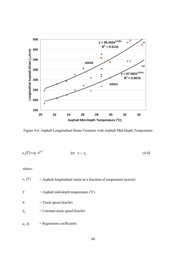
68

Tb

x eaT 11)( for oSS

( 4-4)

where:

)(Tx

= Asphalt longitudinal strain as a function of temperature (m/m)

T

= Asphalt mid-depth temperature (oC)

S

= Truck speed (km/hr)

oS = Constant truck speed (km/hr)

11 ,ba



y = 95.452e0.048x

R2 = 0.9115

y = 67.562e0.051x

R2 = 0.9075

150

200

250

300

350

400

450

500

20 22 24 26 28 30 32 34

Asphalt Mid-Depth Temperature (oC)

Lo

ng

itu

din

al A

sph

alt

Str

ain

(

mm

)

ASG1

ASG5

69

For a truck speed of 25km/hr and wheel load of 49kN, a1 values were found to be 67.6 and 95.5

for ASG1 and ASG5 respectively, and b1 constants were found to be 0.051 and 0.048. It should

be noted that ASG1 and ASG5 have approximately the same b1 constants.

4.5.2 Effect of Truck Speed on Measured Asphalt Longitudinal Strains

To determine the impact of truck speed changes on the measured asphalt longitudinal strain with

a constant wheel load, test data from the following test configuration were used - dual tires

(11R22.5D) with a tire inflation pressure of 689kPa and a wheel load of 49kN moving directly

over the sensors at a speed of 5, 25 and 40 km/hr and 32oC asphalt temperature. Figure 4-7

shows maximum ASG1 and ASG5 asphalt longitudinal strain gauge readings under the three

truck speeds. This figure shows that under a constant temperature of 32oC, the asphalt

longitudinal strains decrease with increasing truck speed.

70

Figure 4-7: Maximum ASG1 and ASG5 Asphalt Longitudinal Strain under Various

Truck Speeds

4.5.3 Truck Speed and Loading Frequency To compare dynamic modulus test data with pavement field response, the loading frequency for

each truck speed was determined. Huang (1993) and Loulizi et al. (2002) reported that the

loading time (duration) of the applied pulse is dependent on the truck speed and the depth

beneath the pavement surface. Figure 4-8 shows the measured vertical stress pulse when the dual

tires (11R22.5D) with a tire inflation pressure of 689kPa and a wheel load of 49kN at a speed of

25km/hr passed over ASG5. TPC1, TPC2, and TPC3 are located 225, 592, and 938mm below

the pavement surface respectively.

71

Figure 4-8: Measured Vertical Stress at TPC1, TPC2, and TPC3

Figure 4-8 confirms that loading time is a function of depth below the asphalt surface as TPC1

has a shorter loading time than TPC3. Since TPC1 is approximately at the same elevation of

ASG1 and ASG5, TPC1 loading time can be used to determine the loading frequency.

Figure 4-9 shows TPC1 vertical stress pulse with a truck speed of 5, 25, and 40 km/hr. This

figure shows that the loading time decreases when the truck speed increases. The shape of the

measured vertical stress pulse was also found to be slightly asymmetrical as the stress pulse tail

was found to be slightly more elongated when the truck moves onto the sensor. Loulizi et al.

(2002) also showed that the stress pulse was slightly asymmetrical. To determine the loading

frequency, the inverse of the loading time, the first half of the stress pulse was used. For truck

TPC1

TPC2 TPC3

72

speeds of 5, 25, and 40km/hr, the loading frequency was determined to be 0.7, 3.5, and 5.5Hz

respectively.

Figure 4-9: TPC1 Vertical Stress under Truck Speed of 5, 25, and 40 km/hr

4.6 Comparison of Dynamic Modulus Test to Pavement Field Response

Equation 4-2, developed using the laboratory dynamic modulus test data, shows that the dynamic

modulus can be represented by an exponential function of temperature when the loading

frequency is constant. Equation 4-4, developed from the controlled wheel load test, also shows

that the asphalt longitudinal strain can be represented by an exponential function of temperature

when the truck speed is constant. It should be noted that Equations 4-2 and 4-4 have the same

form, and Table 4-2 shows that the b values are approximately -0.050 when the frequency is 10

Hz or less. Figure 4-6, developed for a constant speed of 25 km/hr (3.5 Hz), also indicates ASG1

5km/hr

25km/hr

40km/hr

73

and ASG5 to have b1 constants of 0.051 and 0.048 respectively. Thus, b constants for the

dynamic modulus test and b1 constant for the wheel load test are similar in magnitude but

opposite in sign. This indicates that the laboratory measured dynamic modulus is inversely

proportional to the field measured longitudinal strain. This is in agreement with Equation 4-1

that shows that the dynamic modulus is inversely proportional to the measured strain.

4.7 Summary and Conclusions The paper presents the results of laboratory measured dynamic modulus tests performed on HL3

asphalt mix and the results of a field controlled wheel load experiments. Using this data the

following conclusions are drawn.

Laboratory dynamic modulus tests show that the dynamic modulus is an exponential function

of the test temperature when loading frequency is constant, and that the dynamic modulus is

a non-linear function of the loading frequency when the test temperature is constant.

Field controlled wheel load tests found that HL3 asphalt longitudinal strain is an exponential

function of pavement mid-depth temperature when the truck speed and wheel loading is

constant, and that the loading time is a function of depth below the pavement surface and

truck speed.

Using the stress pulse of the pressure cell at the elevation of the asphalt strain gauges the

frequency of loading was found for three truck speeds and that the laboratory dynamic

modulus is inversely proportional to the field measured asphalt longitudinal strain. This

indicates that the dynamic modulus can simulate the pavement behavior under wheel load.

74

4.8 Acknowledgment The authors would like to thank the Natural Science and Engineering Research Council of

Canada (NSERC) and CPATT for providing research funding. We would also like to

acknowledge the Ministry of Transportation Ontario (MTO), Challenger Motor Freight Inc., and

Michelin Canada for their help in organizing and developing the 2006 field test program.

75

Chapter 5: Investigation of Flexible Pavement Structural Response for the Centre for Pavement and Transportation Technology (CPATT) Test Road

5 Investigation of Flexible Pavement Structural Response for the Centre for Pavement and Transportation Technology (CPATT) Test Road

76

5.1 Overview This study was conducted to investigate structural responses of flexible pavements at the Center

for Pavement and Transportation Technology (CPATT) test track located at Waterloo, Ontario,

Canada. A comprehensive field testing program was carried out to examine flexible pavement

responses to a variety of loading conditions. Tests were completed using six tire types: 11R22.5,

275/80R22.5, 295/75R22.5, and 285/70R22.5 dual tires, and 455/55R22.5 and 445/50R22.5

wide-base tires, and tire inflation pressures ranged from 482 to 827kPa. A two dimensional finite

element model was developed using MichPave to predict pavement responses. A simplified

method was proposed to characterize HMA properties using the laboratory dynamic modulus

test. The developed model simulations approximated the field measured responses to all loading

configurations.

77

5.2 Introduction Mechanistic-Empirical (M-E) methods for the design of flexible pavements have gained

significant interest and continue to advance toward full implementation by transportation

agencies (Selvaraj 2007). The response models that predict pavement response (i.e., stress, strain,

and deflection) under traffic loads and/or environmental conditions are the core component of

the M-E design procedure (NCHRP 2004). Therefore, the validity of response models is an

important prerequisite for reliable design and performance prediction of the flexible pavement.

Traditionally, the common practice is to use multi-layered elastic theory to predict pavement

responses under wheel load. Concerns regarding accuracy of this type of model arise when

considering Hot Mix Asphalt (HMA) materials which exhibit viscoelastic behavior and dynamic

loads which are applied by moving traffic (Liao 2007). Over the years, numerous finite element

(FE) models, capable of modeling viscoelastic HMA behavior and performing dynamic analysis,

have been developed (Loulizi et al. 2006) . However, the application of these programs requires

considerable expertise from the user and demands a large amount of computation time.

Therefore, the layered elastic models continue to be the state-of-the practice for most pavement

design and analysis applications (Selvaraj 2007).

In 2006, a series of controlled loading tests were performed at the Center for Pavement and

Transportation Technologies (CPATT) test track to investigate pavement dynamic response due

to various loading conditions. This paper discusses field controlled wheel load experiments

performed at the CPATT test track facility and presents the asphalt longitudinal strain responses.

It also explains a three step procedure implemented to simplify incorporating laboratory

determined viscoelastic properties of HMA into a finite element (FE) model to accurately

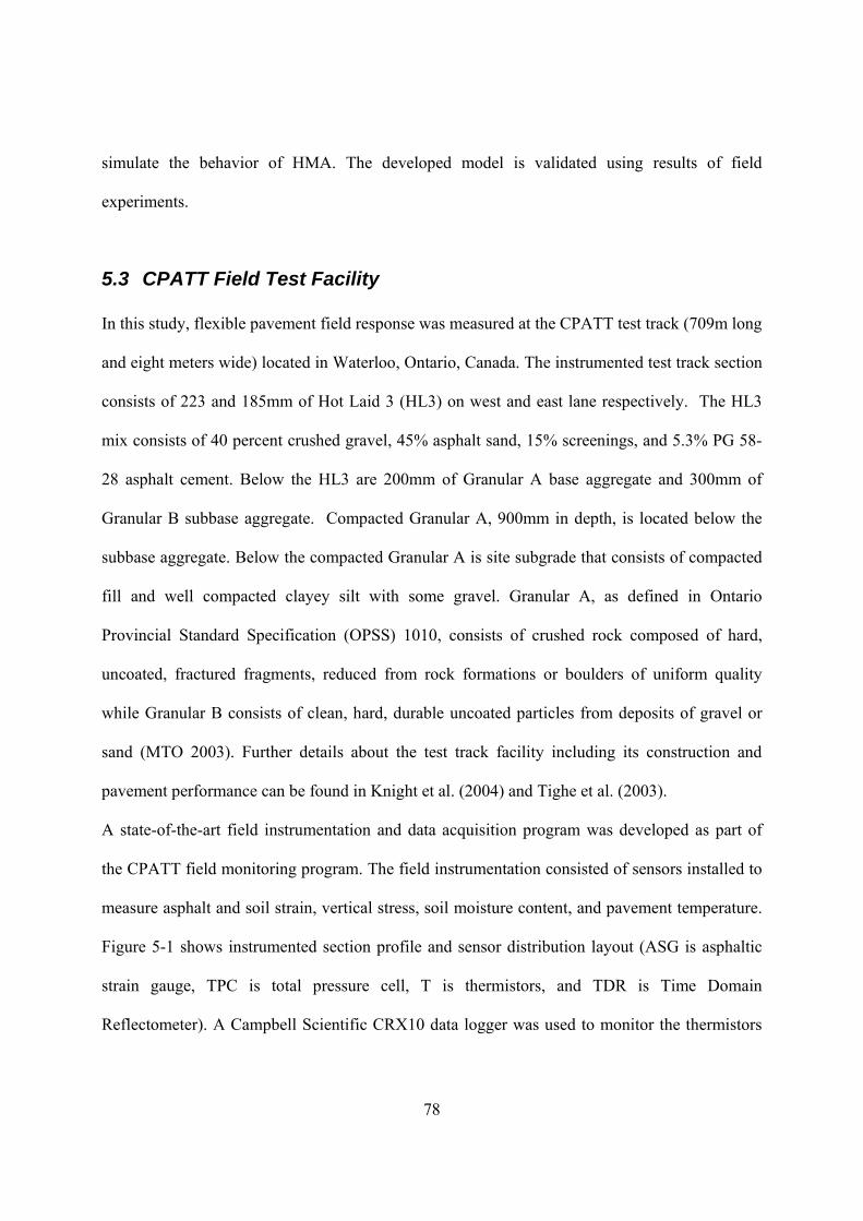
78

simulate the behavior of HMA. The developed model is validated using results of field

experiments.

5.3 CPATT Field Test Facility In this study, flexible pavement field response was measured at the CPATT test track (709m long

and eight meters wide) located in Waterloo, Ontario, Canada. The instrumented test track section

consists of 223 and 185mm of Hot Laid 3 (HL3) on west and east lane respectively. The HL3

mix consists of 40 percent crushed gravel, 45% asphalt sand, 15% screenings, and 5.3% PG 58-

28 asphalt cement. Below the HL3 are 200mm of Granular A base aggregate and 300mm of

Granular B subbase aggregate. Compacted Granular A, 900mm in depth, is located below the

subbase aggregate. Below the compacted Granular A is site subgrade that consists of compacted

fill and well compacted clayey silt with some gravel. Granular A, as defined in Ontario

Provincial Standard Specification (OPSS) 1010, consists of crushed rock composed of hard,

uncoated, fractured fragments, reduced from rock formations or boulders of uniform quality

while Granular B consists of clean, hard, durable uncoated particles from deposits of gravel or

sand (MTO 2003). Further details about the test track facility including its construction and

pavement performance can be found in Knight et al. (2004) and Tighe et al. (2003).

A state-of-the-art field instrumentation and data acquisition program was developed as part of

the CPATT field monitoring program. The field instrumentation consisted of sensors installed to

measure asphalt and soil strain, vertical stress, soil moisture content, and pavement temperature.

Figure 5-1 shows instrumented section profile and sensor distribution layout (ASG is asphaltic

strain gauge, TPC is total pressure cell, T is thermistors, and TDR is Time Domain

Reflectometer). A Campbell Scientific CRX10 data logger was used to monitor the thermistors

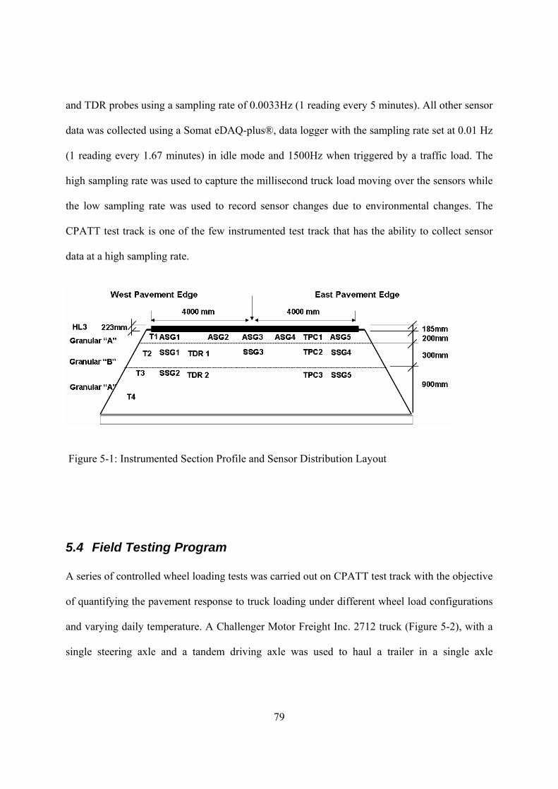
79

and TDR probes using a sampling rate of 0.0033Hz (1 reading every 5 minutes). All other sensor

data was collected using a Somat eDAQ-plus®, data logger with the sampling rate set at 0.01 Hz

(1 reading every 1.67 minutes) in idle mode and 1500Hz when triggered by a traffic load. The

high sampling rate was used to capture the millisecond truck load moving over the sensors while

the low sampling rate was used to record sensor changes due to environmental changes. The

CPATT test track is one of the few instrumented test track that has the ability to collect sensor

data at a high sampling rate.


5.4 Field Testing Program A series of controlled wheel loading tests was carried out on CPATT test track with the objective

of quantifying the pavement response to truck loading under different wheel load configurations

and varying daily temperature. A Challenger Motor Freight Inc. 2712 truck (Figure 5-2), with a

single steering axle and a tandem driving axle was used to haul a trailer in a single axle

80

configuration so that the outer trailer tire passed over ASG1 and ASG5 at a targeted speed of 5,

25 and 40km/hr.

Figure 5-2: Challenger Motor Freight Inc. 2712 Truck Used for Field Test

The trailer was configured so that a single axle load could be quickly adjusted to prescribed

values between 7,000 to 15,000kg. All axle loads were set using a mobile scale placed under

each axle tire. Multiple passes of the truck were collected for each load configuration to ensure at

least three wheel loads passed over the sensors. Video cameras along with pavement markings

were used to verify when a wheel passed directly over each strain gauge. For each axle load and

tire configuration the tire contact area was measured by obtaining a static tire imprint. Pressure-

sensing pads were also used to determine the tire static contact pressure.

81

The vertical stress and asphalt longitudinal strains were measured and recorded at a frequency of

1500Hz for each wheel pass. Test Control software (TCE) was used to set up test requirements in

eDAQ data acquisition system and to specify triggering conditions for collection of test data. The

recorded high speed signals were processed using Infield Somat field analysis software program

that is optimized for use with Somat hardware. This software allowed for quick analysis of the

large data files. Typical asphalt longitudinal strain gauge and total pressure cell data are shown in

Figure 5-3 and Figure 5-4 respectively.

Figure 5-3 shows ASG5 longitudinal strain measured at the bottom of asphalt layer under a

wheel load of 49kN moving at a speed of 25km/hr. The first pulse, at 1 second, represents the

passing of the truck steering axle over the strain gauge. The following two pulses, at

approximately 1.4 and 1.6 seconds, are the truck’s dual tandem drive wheels passing over the

strain gauge. The third pulse, at approximately 3.2 seconds, represents the passing of the

prescribed trailer wheel load.

82


Trailer Wheel Loads

Figure 5-4 Total Pressure Cell (TPC1) Response during the Passing of the truck and Trailer

Wheel Loads

83

Figure 5-4 shows TPC1 vertical stress when the truck and trailer with a 49kN wheel load passed

over ASG5 at a speed of 25km/hr. The first peak pressure response, at approximately 1 second,

represents the passing of the steering axle while the two following pressure peaks represent the

passing of the truck dual tandem drive wheels. The third pressure peak, at approximately 3.3

seconds, represents the passing of the prescribed trailer wheel load.

Tests were completed using six tire types: 11R22.5, 275/80R22.5, 295/75R22.5, and

285/70R22.5 dual tires, and 455/55R22.5 and 445/50R22.5 wide-base tires. Tire inflation

pressures ranged from 482 to 827kPa. Table 5-1 to Table 5-4 summarize the test configuration

and ASG1 and ASG5 maximum asphalt longitudinal strain for each loading configuration.

ASG1 has consistently lower strain than ASG5. This lower measured strain is inferred to be the

result of the west lane asphalt being 38mm thicker than the east lane. The asphalt mid-depth

temperature was determined by averaging the measured asphalt surface temperature and the

temperature measured at the base of the asphalt layer (T-1).

84

Table 5-1: Test Configuration and Asphalt Strain Gauge Response- 455/55R22.5 Wide Base

Tire

Tire Pressure

Maximum Asphalt Longitudinal Strain

(m/m) Run ID

Wheel Load (kg)

psi kPa

Truck Speed

(km/hr)

Mid-Depth Temp. (oC)

ASG1 ASG5

1 4525 110 758.4 25.5 23.2 240.7 339.9

11 5025 125 861.8 24.7 22.3 243.8 351.1

12 4500 110 758.4 25.5 24.6 237.4 351.0

13 4085 95 655.0 25.3 26.4 241.1 350.0

14 3500 80 551.6 24.3 28.9 238.5 347.2

25-6 4450 110 758.4 26.0 29.3 293.0 441.0

35 4450 110 758.4 5.0 30.1 398.0 623.0

37 4450 110 758.4 35.7 29.9 310.0 443.0

85

Table 5-2: Test Configuration and Asphalt Strain Gauge Response- 445/50R22.5 Wide Base

Tire

Tire Pressure


(m/m) Run ID

Wheel Load (kg)

psi kPa

Truck Speed

(km/hr)

Asphalt Mid-Depth

Temp. (oC) ASG1 ASG5

16 4540 115 792.9 25.0 33.6 390.8 542.0

17 4100 100 689.5 25.3 31.9 338.5 482.4

18 3500 85 586.1 25.7 31.3 285.8 412.1

27-8 4450 110 758.4 27.1 26.9 249.0 409.0

86

Table 5-3: Test Configuration and Asphalt Strain Gauge Response- 11R22.5 Dual

Tire

Tire Pressure


(m/m) Run ID

Wheel Load (kg)

psi kPa

Truck Speed

(km/hr)

Asphalt Mid-Depth

Temp. (oC)

ASG1 ASG5

2 4000 70 482.6 25.3 26.0 204.3 267.1

3 4550 85 586.1 24.5 28.0 288.6 379.0

4 5025 100 689.5 23.6 28.0 316.8 410.0

5 5500 115 792.9 24.2 29.5 346.8 437.5

6 6100 120 827.4 25.1 28.4 336.1 448.4

7 6560 120 827.4 25.4 27.0 332.3 422.3

10 5025 100 689.5 23.3 19.7 183.2 248.2

15 5000 100 689.5 25.1 34.2 368.0 473.0

23 4960 100 689.5 25.3 22.1 205.0 277.0

41 4900 100 689.5 5.0 31.9 481.0 597.0

50 4925 100 689.5 39.6 30.1 325.0 430.0

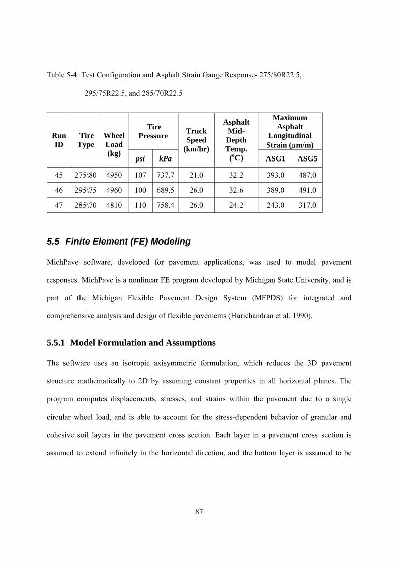
87

Table 5-4: Test Configuration and Asphalt Strain Gauge Response- 275/80R22.5,

295/75R22.5, and 285/70R22.5

Tire Pressure

Maximum Asphalt

Longitudinal Strain (m/m)

Run ID

Tire Type

Wheel Load (kg)

psi kPa

Truck Speed

(km/hr)

Asphalt Mid-Depth Temp.

(oC) ASG1 ASG5

45 275\80 4950 107 737.7 21.0 32.2 393.0 487.0

46 295\75 4960 100 689.5 26.0 32.6 389.0 491.0

47 285\70 4810 110 758.4 26.0 24.2 243.0 317.0

5.5 Finite Element (FE) Modeling MichPave software, developed for pavement applications, was used to model pavement

responses. MichPave is a nonlinear FE program developed by Michigan State University, and is

part of the Michigan Flexible Pavement Design System (MFPDS) for integrated and

comprehensive analysis and design of flexible pavements (Harichandran et al. 1990).

5.5.1 Model Formulation and Assumptions The software uses an isotropic axisymmetric formulation, which reduces the 3D pavement

structure mathematically to 2D by assuming constant properties in all horizontal planes. The

program computes displacements, stresses, and strains within the pavement due to a single

circular wheel load, and is able to account for the stress-dependent behavior of granular and

cohesive soil layers in the pavement cross section. Each layer in a pavement cross section is

assumed to extend infinitely in the horizontal direction, and the bottom layer is assumed to be

88

infinitely deep. All the pavement layers are assumed to be fully bonded so that no interlayer slip

occurs due to applied load (Harichandran et al. 1990).

MichPave uses rectangular four-nodded elements with linear interpolation functions

(Harichandran et al. 1990). A lateral boundary is placed at a radial distance of 15a to 40a from

the center of the wheel contact area, where a is the radius of the wheel contact area. A default

mesh generation is used for the analysis, but it can be modified when necessary. Figure 5-5

shows the developed FE mesh in MichPave.

The default mesh has the following characteristics:

In the radial direction, the total width is divided into four regions: 0 to a, a to 3a, 3a to 6a,

and 6a to the lateral boundary. All elements within a region have the same horizontal

dimension. The default location of the lateral boundary varies from 15a to 40a depending on

the thickness of the asphalt concrete layer.

Within any layer, all elements have the same vertical dimension.

The aspect ratio of all elements is less than 1:4.

89

Figure 5-5: MichPave Finite Element Mesh- East Lane

5.5.2 HMA Modulus Characterization MichPave treats HMA as an elastic material and uses resilient modulus for HMA

characterization. However, unlike elastic solids, the HMA materials are viscoelastic and their

behavior depends strongly on temperature and loading frequency. In this study, the dynamic

modulus test was chosen to determine viscoelastic properties of HMA material. A three step

procedure was proposed and used to incorporate laboratory determined viscoelastic properties of

HMA into the MichPave FE Model. The implemented procedure is as follows:

5.5.2.1 Step 1: Laboratory HL3 Dynamic Modulus under Various Temperature and

Loading Frequencies

90

The laboratory dynamic modulus test data was used to determine the HL3 dynamic modulus

under different temperature and loading frequencies. Uzarowsky (2006) presents the results of

dynamic modulus tests performed on several mixes including HL3 - the mix used in the

instrumented section of CPATT test track. The HL3 mix was designed using the Marshall

methodology to meet requirements of OPSS 1150 (MTO 2003). HL3 specimens, 150mm in

diameter, were constructed in accordance with AASHTO TP62-03 standard (AASHTO 2003)

using a Superpave Gyratory Compactor. Dynamic modulus test specimens, 100 mm in diameter,

were cored from the 150mm specimens. The measured average air void was determined to be 6.2

percent. An Interlaken UniTest Control System with pre-programmed software was used to

determine the dynamic modulus of HL3 at five testing temperatures (-10, 4.4, 21.1, 37.8, and

54.4oC) and six loading frequencies (0.1, 0.5, 1.0, 5.0, 10.0, and 25.0Hz). HL3 dynamic modulus

( *E ) test results reported by Uzarowsky (2006) are summarized in Table 5-5.

Table 5-5: HL3 Dynamic Modulus (Uzarowsky (2006))

Dynamic Modulus (MPa) Loading Frequency

(Hz) -10oC 4.4 oC 21.1 oC 37.8 oC 54.4 oC

25 29035.6 18234.1 8517.0 3677.7 1771.9

10 26140.9 15782.4 6724.6 2531.6 1241.3

5 23758.5 14155.5 5632.2 2001.5 1062.6

1 19463.9 8970.2 3567.4 1324.5 789.3

0.5 17024.6 8410.7 2903.3 1139.1 723.1

0.1 12462.5 5904.9 1923.6 876.3 543.0

Figure 5-6 shows changes in dynamic modulus with temperature for each loading frequency.

91

Figure 5-6: Dynamic Modulus versus Temperature for Each Loading Frequency.

5.5.2.2 Step 2: Wheel Load Frequency for Each Truck Speed

For each truck speed, loading frequency was determined using the TPC1 pressure wave. Huang

(1993) and Loulizi et al. (2002) report that the loading time (duration) of the applied pulse is

dependent on the truck speed and the depth beneath the pavement surface. Since TPC1 is at the

same elevation as ASG1 and ASG5, TPC1 loading time can be used to determine the frequency

of loading. Figure 5-7 shows TPC1 vertical stress pulse with a truck speed of 5, 25, and 40 km/hr

when the dual tires (11R22.5D) with a tire inflation pressure of 689kPa and a wheel load of

49kN passed over ASG5. This figure shows that the loading time decreases with an increase in

truck speed.

92

The shape of the measured vertical stress pulse was found to be slightly asymmetrical. When the

truck moves away from the sensor the stress pulse tail was found to be slightly more elongated

than when the truck moves onto the sensor. Loulizi et al. (2006) also showed that the stress pulse

was slightly asymmetrical. To determine the loading frequency, the inverse of the loading time,

the first half of the stress pulse was used. For truck speeds of 5, 25, and 40km/hr, the loading

frequency was determined to be 0.7, 3.5, and 5.5Hz respectively.

Figure 5-7: TPC1 Vertical Stress under Truck Speed of 5, 25, and 40 km/hr

5.5.2.3 Field Represented Dynamic Modulus Changes in dynamic modulus with temperature for loading frequency of 0.7, 3.5, and 5Hz were

interpolated using the data shown in Table 5-5 (Figure 5-6).

5km/hr

25km/hr

40km/hr

93

Asphalt mid-depth temperature was determined by averaging the measured asphalt surface

temperature and the temperature measured at the base of the asphalt layer (T-1). Table 5-1 to

Table 5-4 present the asphalt mid-depth temperature for each loading configuration.

Figure 5-8: HL3 Dynamic Modulus under Loading Frequency of 0.7, 3.5, and 5 Hz

(Corresponding to Truck Speed of 5, 25, and 40 km/hr)

Figure 5-8 was used to calculate the field represented dynamic modulus using asphalt mid-depth

temperature and loading frequency (truck speed). The field represented dynamic modulus was

then used as an elastic modulus of HMA in FE analysis.

5.5.3 Granular Material Characterization The so-called K-3 model was used to characterize the resilient modulus of granular materials.

This model is of the form:

94

2

31K

R KM

( 5-1)

where:

RM = Resilient Modulus (MPa)

3 = Confining pressure (MPa)

21, KK = Constant values

The average in-situ density of the soil immediately below the subbase and on top of the subbase

was determined to be 20.5 and 21.75 kN/m3 respectively. The material properties assigned to the

Granular A and Granular B, shown in Table 5-6, were obtained from the results of extensive

laboratory tests on compacted soils published by Selig (1988).

Table 5-6: Summary of Granular Material Properties Used for Simulation

Soil Type

Properties Granular A Granular B

K1 5994 8834

K2 0.6 0.43

Friction Angle (degree) 48 42

Density (kg/m3) 2200 1800

95

5.6 Validation of the FE model Calculated asphalt longitudinal strains from FE model were compared to field measurements,

and the results are shown in Figure 5-9 to Figure 5-12.


455/55R22.5 Wide Base Tire

96

Figure 5-10: Comparison of Field Measured and Calculated Asphalt Longitudinal Strain

- 445/55R22.5 Wide Base Tire

97


- 11R22.5 Dual Tire

98


- 275/80R22.5, 295/75R22.5, and 285/70R22.5

It can be seen that overall the FE model yielded reasonably close predictions compared with field

measured values.

5.7 Summary and Conclusions The paper presents the results of field controlled wheel load experiments performed at CPATT

test track. The following conclusions are drawn. Tests were completed using six tire types:

11R22.5, 275/80R22.5, 295/75R22.5, and 285/70R22.5 dual tires, and 455/55R22.5 and

445/50R22.5 wide-base tires, and tire inflation pressures ranged from 482 to 827kPa. A two

dimensional FE model was developed using MichPave to predict pavement responses. A three

99

step procedure was implemented to incorporate laboratory determined viscoelastic properties of

HMA into the model. The developed model was validated using the result of field experiments.

The results demonstrated that the developed simplified method for incorporating laboratory

determined viscoelastic properties of HMA into FE model can predict pavement responses

accurately.

5.8 Acknowledgements The authors acknowledge the Natural Sciences and Engineering Research Council of Canada

(NSERC), Canada Foundation for Innovation (CFI), Ontario Innovation Trust (OIT), Ontario

Research and Development Challenge Fund (ORDCF), along with the Center for Pavement and

Transportation Technologies (CPATT) private and public sector partners for providing research

funding. The authors also acknowledge the University of Waterloo technical staff, Ken Bowman,

Terry Ridgway, and Doug Hirst, for their guidance, help, and assistance with the field

instrumentation.

100

Chapter 6: Long-Term Monitoring of Environmental Parameters to Investigate Flexible Pavement Response

6 Long-Term Monitoring of Environmental Parameters to Investigate Flexible Pavement Response

101

6.1 Overview A research program is developed and implemented in a climate subjected to freeze-thaw cycles

to investigate the impact of environmental parameters on flexible pavement response. Details of

the field data collection system implemented at the Centre for Pavement and Transportation

Technologies (CPATT) field test facility located in Waterloo, Ontario, Canada are presented.

Data processing and data analysis are also discussed. Temperature, soil moisture content, asphalt

longitudinal strain, Falling Weight Deflectometer (FWD), and resilient modulus readings

recorded over a two year period are presented and discussed. Field results presented in this study

show that: 1) the pavement is subjected to several freeze-thaw cycles during the winter months;

2) rapid fluctuations occur in the soil moisture probe readings when the ground is subjected to

freeze-thaw cycles; 3) FWD and soil resilient modulus are highly correlated to soil moisture

content; 4) asphalt longitudinal strain fluctuated between 600 and 650m/m during spring and

summer months.

102

6.2 Introduction Pavement response has been shown to be correlated to environmental conditions, such as

moisture content and temperature (Salem 2004; Zuo 2003). Akhter and Witczak (1985), Drumm

et al. (1997), Li and Selig (1994), and Park et al. (2001) report that moisture content influences

unbound material modulus and temperature influences asphalt stiffness and pavement response.

Al-Qadi et al. (2005), Monismith et al. (1966), and Haas (1968) also report that temperature

changes induce asphalt strains. Field monitoring programs have been used to understand

pavement response due to environmental conditions (Salem 2004; Zuo 2003). To date most

published field studies have been completed in relatively mild climatic conditions (Watson and

Rajapakse 2000). Limited published environmental data exist for pavements subjected to

climates with freeze-thaw cycles (such as southern Canada).

A field investigation program was developed at the University of Waterloo to investigate in-situ

flexible pavement response due to environmental conditions in a climate subjected to freeze-

thaw cycles. Figure 6-1 shows the overall field program implemented at the test track facility

located in Waterloo, Ontario, Canada. The primary objectives of the investigation program were:

(i) monitor and measure daily and seasonal changes in moisture and temperature of the pavement

structure and (ii) evaluate pavement response (i.e. deflections and strains) due to changes in soil

moisture and air temperature. To ensure a successful data collection system, the following

components were considered: 1) sensors must be compatible with the research objectives; 2)

sensors need to be calibrated prior to installation; 3) the data acquisition system (DAS) must be

compatible with sensors; and 4) DAS must have the ability to monitor and record sensors

readings at the required frequency.

103

Figure 6-1: Research Process

For this study, the DAS had the ability to collect load sensor data at a high frequency and

environmental sensor data at low frequency. For long-term field monitoring in remote locations,

power supply and management play a critical role in the successful operation and collection of

sensor data. To effectively and efficiently analyze large data sets, careful consideration must be

given to data formats and to the selection of specialized software tools.

104

This paper provides an overview of the field test facility, and the data collection, processing, and

analysis. Two years of environmental data that has freeze-thaw cycles is also presented and

discussed.

6.3 Site Information In this study, environmental parameters and flexible pavement field response was measured at

the CPATT test track (709m long and eight meters wide) located in Waterloo, Ontario, Canada.

The two lane CPATT test track has asphalt overlay consisting of binder Hot Laid 3 (HL3) plus a

surface mix consisting of HL3, Polymer-Modified Asphalt (PMA), and Stone Mastic Asphalt

(SMA) or Superpave. Figure 6-1 shows the location and arrangement of each surface mix.

The instrumented test track section consists of 223 mm and 185 mm of HL3 on the west and east

lane respectively. The HL3 mix consists of 40 percent crushed gravel, 45% asphalt sand, 15%

screenings, and 5.3% PG 58-28 asphalt cement. Below the HL3 are 200mm of Granular A base




defined in the Ontario Provincial Standard Specification (OPSS) 1010, consists of crushed rock

composed of hard, uncoated, fractured fragments, reduced from rock formations or boulders of


deposits of gravel or sand (MTO 2003). Further details about the test track facility including its

construction and pavement performance can be found in Tighe et al. (2003).

105

Figure 6-2: CPATT Test Track Facility Located at Waterloo Region

6.4 Data collection

6.4.1 Sensors A state-of-the-art field instrumentation system was developed and installed to measure

environmental conditions and pavement structural responses. Environmental measurements

pertinent to this work included temperature of the asphalt, base, and subgrade materials, and

moisture content of the base and subgrade layers. Time Domain Reflectometr (TDR 1 and TDR

2) probes and thermistors (T-1 to T-4) were installed, as shown in Figure 6-3, to measure

moisture and ground temperatures, respectively.

Equipment andData Logging Trailer

HL3-2 Superpave SMA PMA HL3-1

East Lane

West Lane

0 m

153

283

420

567

709

m

425 36

335

8

284 22

0

155

122.

8

Weight in Motion Scale

Geogrid

Location of Instrumentation

Equipment andData Logging Trailer

HL3-2 Superpave SMA PMA HL3-1

East Lane

West Lane

0 m

153

283

420

567

709

m

425 36

335

8

284 22

0

155

122.

8

Weight in Motion Scale

Geogrid

Location of Instrumentation

106

Figure 6-3: Pavement Profile and Environmental Sensor Distribution

Instrumentation also included asphalt strain gauges (ASG1 to ASG5), as shown in Figure 6-4, to

measure asphalt longitudinal strain. The following sections, adopted from Adedapo (2007),

provide details of the environmental and load sensors.

6.4.1.1 Time-Domain Reflectometry Probes (TDR) To measure base and subbase daily and seasonal moisture content changes, two Campbell

Scientific CS616 TDR probes (TDR1 and TDR2) were installed respectively 800 and 1150mm

below the west lane asphalt surface. The TDR probes were selected due to their performance,

survivability, cost, and ability to integrate with available existing data acquisition loggers. The

TDR probes consisted of two parallel conducting rods, 300mm in length, with a separation

distance of 32mm. All sensors were calibrated prior to installation using site Granular A and B

aggregates.

107

Figure 6-4: Asphalt Strain Gauge Distribution

6.4.1.2 Temperature Probes Four Campbell Scientific T107B thermistors (T-1 to T-4) were installed 223, 530, 1134, and

1734mm below the west lane asphalt surface. Campbell Scientific reports the thermistors

precision to be 0.1 °C between -35° to 50°C.

6.4.1.3 Asphalt Strain Gauges (ASG) To measure asphalt longitudinal strains at the base of the asphalt layer, five ASG-152 H-type

asphalt strain gauges, manufactured by Construction Technology Laboratories (CTL) Group Inc.,

were installed. These gauges were chosen due to their reliability, durability, low cost, short

delivery time, and excellent performance at other test sites. Prior to installation, each gauge’s

calibration and functionality was checked in the laboratory. As shown in Figure 6-4, ASG3 was

placed on the road centerline, while ASG1 and ASG2 were placed 690 and 2700mm from the

west pavement edge respectively. ASG5 and ASG 4 were placed 1380 and 3200mm from the

east pavement edge respectively. To ensure that the asphalt strain gauges were bound to the

108

asphalt base course, all asphalt strain gauges were placed in a sand-asphalt binder mixture

consisting of sand and PG 64-22 binder.

6.4.2 Data Acquisition Systems (DAS) A Campbell Scientific CRX10 data logger was used to monitor the thermistors and TDR probes

using a sampling rate of 0.0033Hz (1 reading every 5 minutes). This sampling rate was deemed

sufficient to record daily sensor changes.

Asphalt strain gauge data was collected using a Somat eDAQ-plus® data logger with the

sampling rate set at 0.01 Hz (1 reading every 1.67 minutes) in idle mode and 1500 Hz when

triggered by a traffic load. The high sampling rate was used to capture the millisecond traffic

load moving over the sensors. The low sampling rate was used to record sensor readings due to

environmental changes. The CPATT test track is unique due to its ability to record sensor data at

low and high frequency. The compact, rugged, and modular Somat eDAQ system has the

capability to collect a wide range of signal types directly from sensors (i.e., strain, analog to

±80V, digital, frequency, and temperature). The eDAQ system used in this study had the

following layers: Base Processor, High Level, and Simultaneous High Level. The Base Processor

has a 266 MHz processor with integrated floating point, master sample clock speed of 100 kHz,

256MB of on board DRAM, and 2GB memory for onboard data storage. The High Level Layer

consists of 16 multiplexed singled-ended channels with a 16 bit A/D converter with a channel-to

channel skew of approximately 25μsec with a maximum sampling rate of 2500Hz. An onboard

excitation source provides ±10V with 30mA output for sensor conditioning. The Simultaneous

High Level layer has 16 general-purpose analog inputs channels. Each input was independently

set to measure down to 3.8μV resolution or have a full-scale input range of ±80 volts. Each

109

channel has its own 16-bit analog-to-digital converter (ADC) running at a frame check sequence

(FCS) master sample clock rate of 100 kHz. The ADCs output was down-sampled to the user-

selected rate between 0.1 to 100,000 samples per second. The settings for full-scale range,

sample rate, digital filtering, and transducer power voltage level was fully independent for each

channel. Each of the 16 channels collected data using different sample rates, digital filters, and

transducer power levels. Transducer power was set from +3V to +28V in one volt increments

with an accuracy of ±50mV. Each channel was power-limited to 400mW. Multiple transducer

power outputs were combined to drive a transducer. Each channel has an input impedance of

10MΩ for ranges up to ±10V and 100kΩ for ranges greater then ±10V. Common mode input

voltages of up to ±80V were provided with 100kΩ input impedance. Small conditioning

modulus, called Smart Modulus, was used to condition strain gauge and thermocouple inputs.

Ethernet 100BaseT and RS232 serial communication provides the PC-to-eDAQ communication.

Test Control software (TCE), a Windows TM based software application, was used to set up and

define test requirements in the eDAQ. This included: creation of the test setup files that define

and calibrate transducer channels; creation of data modes and computed channels for online data

calculations and analyses; specification of triggering conditions for collection of sensor data;

sensor monitoring via run-time displays; and initialization, starting, stopping, and uploading of

sensor stored data.

6.4.3 Power Supply and Management For long-term field monitoring in remote locations, power supply and management play a crucial

role for the operation and collection of sensor data. For this project, power was supplied using

two 12V deep cycle batteries that were recharged using a solar panel (Figure 6-5).

110

Figure 6-5: Solar Panel for Recharging Batteries at Test Site (Adedapo 2007)

To conserve battery power during the winter time - when the duration of solar recharge was

limited - a programmable timer was used to automatically turn the system off and on at

predefined times. A power regulator was also used to prevent batteries from overcharging and

discharging, and to prevent power flow from the batteries to the solar panel. Safety disconnect

switches were installed so that the system power could be turned off without the need to

disconnect wires. This power system was found to work well, be robust, and a cost effective

method to power the sensors, Somat eDAQ-plus®, and Campbell Scientific CRX10.

6.4.4 Remote Monitoring System A unique remote monitoring system was developed to allow the monitoring of the eDAQ field

computer and the downloading of the sensor data over a secure internet connection. Figure 6-6

shows the secure remote monitoring system used at the site.

111

This remote monitoring system allowed for daily data upload and the ability to check sensor

functionality without the need to travel to the site. During one data check, several asphalt strain

gauges were found not to be functioning. After a site visit it was found that sensors wires had

been accidentally cut during grass mowing. All wires were promptly fixed resulting in only a

short period of limited data collection. The Campbell Scientific CRX10 data was downloaded

manually on a weekly basis.

6.4.5 Pavement Response Surveys Falling Weight Deflectometer (FWD) pavement surveys were performed by Applied Research

Associates Inc. along the test track at 20m intervals Details on the pavement condition and

performance were reported by Popik and Tighe (2006). FWD test results for each survey station

include back calculated subgrade resilient modulus.

112


6.5 Data Processing Field monitoring programs require the ability to store and to efficiently process large volumes of

data. For this study, approximately 5 gigabytes/year of field data was collected. Somat InField

and MS Excel programs were used to process and display the results of the load and

environmental sensors.

Asphalt strain gauge data were processed with SoMat InField, a versatile, powerful software

application optimized for use with the eDAQ data acquisition system. Infield allows sensor data

to be read from the eDAQ file (.SIF) and displayed graphically. It also contains different data

processing functions that allow for easy data combining and exporting of approximately 87,500

113

data files that represent 8 million data points to MS Excel. MS Excel macros were used to extract

and process sensor data.

Campbell Scientific CRX10, TDR, and thermistors data files (.DAT) were imported into MS

Excel for data processing. A database that has 210,240 data points was constructed, and MS

Excel macros were developed to extract and process the data.

6.6 Data Analysis

6.6.1 Ground and Ambient Air Temperature Variation Figure 6-7 to Figure 6-10 show ground and ambient air temperature variation for the period from

April 2004 to May 2005. Ambient air temperature data was obtained from the University of

Waterloo weather station, located approximately five kilometers north east of the CPATT test

site. The March 2005 data gap, shown in Figure 6-7 to Figure 6-10, corresponds to a period of 13

days when the Campbell Scientific CRX10 data logger was removed from the site.

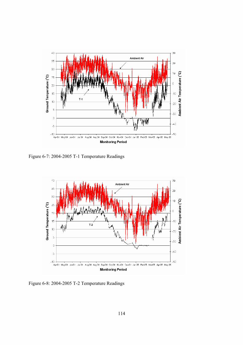
114

Figure 6-7: 2004-2005 T-1 Temperature Readings


115



116

All temperature probes show a sinusoidal response with decreasing temperature variation and

sensitivity with depth. For example, temperature probe T-1, located 223mm below the asphalt

layer, has a temperature variation of 38°C with daily temperature fluctuations of 10 to 20°C

while T-4 shows a temperature variation of 17 °C with daily temperature fluctuations of 1°C.

Figure 6-7 shows that T-1 recorded freezing ground conditions from November to the end of

March while Figure 6-8 and Figure 6-9 indicate freezing or near freezing ground conditions

starting in late December to early January respectively. Figure 6-10 indicates no ground freezing

occurred at 1734mm. Thus, the frost depth was between 1134 and 1734mm below the asphalt

surface.

6.6.2 Average Daily Temperature Figure 6-11 shows the average daily temperature with depth below the asphalt surface and the

average ambient air temperature from April 2004 to March 2005. This figure shows that all

average daily temperatures have a response similar to the average ambient air temperature, and

that the average ambient air temperature was always lower than the average ground temperature

for T-1, T-2, and T-3. It also shows that during the warming period from April 2004 until

September 2004 the average daily temperature decreases with depth. Therefore, the ground has a

temperature gradient. In September 2004, the average daily temperature was constant resulting in

a negligible temperature gradient (all temperature probes had average value of 17.5 oC). After

September 2004, the average ground temperature was found to increase with depth. Thus, the

ground has a reversed temperature gradient compared to the period prior to September 2004.

This reversed temperature gradient continues until March 2005, when the average daily

temperature becomes constant (all temperature probes had average value of 4 oC).

117

-10

-5

0

5

10

15

20

25

Mar-04 Apr-04 May-04 Jun-04 Jul-04 Aug-04 Sep-04 Oct-04 Nov-04 Dec-04 Jan-05 Feb-05 Mar-05 Apr-05

Monitoring Period

Ave

rag

e D

aily

Tem

per

atu

re (

oC

) T-1

T-2

T-3

T-4

Ambient Air Temperature

Figure 6-11: 2004-2005 Average Daily Ambient Air Temperature and Average Daily

Ground Temperature below the Asphalt

6.6.3 Moisture Content Variation over Monitoring Period Figure 6-12 shows TDR1 (upper) and TDR2 (lower) seasonal moisture content changes from

March 2004 to February 2006. The small data gap, in March 2005, corresponds to a period of 13

days when the Campbell Scientific CRX10 data logger was removed from the site.

118

Figure 6-12: 2004-2005 TDR1 and TDR2 Soil Moisture Content Readings

Both TDR probes showed the following response:

Maximum soil moisture occurred during March to April.

Soil moisture decreased from April to October.

Soil moisture increased from October to November/December.

Soil moisture showed a period of high and low moisture content when the ground freezes

and thaws during the winter months (November to February).

During the monitoring period, TDR1 indicated soil moisture content between 5 to 22 percent

while TDR2 had soil moisture content between 17 to 25 percent.

119

6.6.4 Moisture and Pavement Performance Variation with Time Figure 6-13 shows soil moisture content and FWD peak deflections from April 2004 to February

2005.

Figure 6-13: Subgrade Resilient Modulus and Soil Moisture Content Readings

The above figure shows an inverse correlation between resilient modulus and moisture content

(i.e., the highest modulus occurs during winter months when the ground is frozen and lowest

occurring during the spring ground thaw). Salem (2004) also reported an inverse correlation

between resilient modulus and soil moisture content. Using a nonlinear regression analysis,

Equation 6-1, with an R2 of 0.91, was found to fit the data.

0694.017.211 eM R

( 6-1)

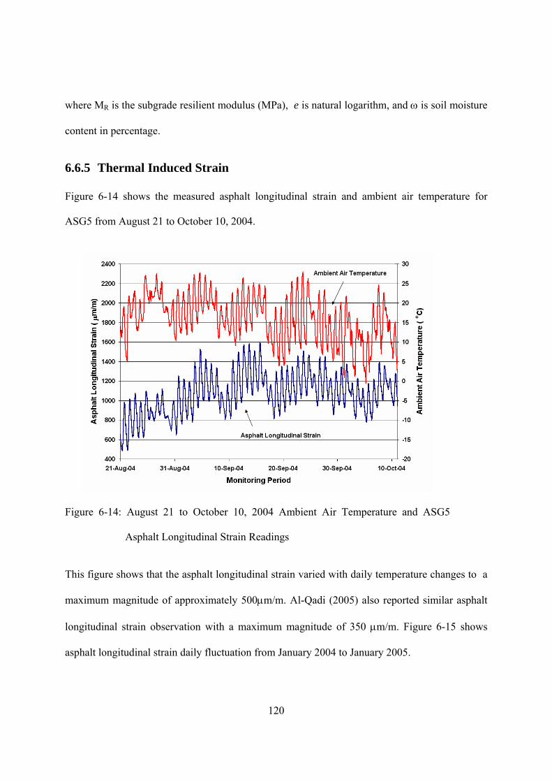
120

where MR is the subgrade resilient modulus (MPa), e is natural logarithm, and is soil moisture

content in percentage.

6.6.5 Thermal Induced Strain Figure 6-14 shows the measured asphalt longitudinal strain and ambient air temperature for

ASG5 from August 21 to October 10, 2004.

Figure 6-14: August 21 to October 10, 2004 Ambient Air Temperature and ASG5

Asphalt Longitudinal Strain Readings

This figure shows that the asphalt longitudinal strain varied with daily temperature changes to a

maximum magnitude of approximately 500m/m. Al-Qadi (2005) also reported similar asphalt

longitudinal strain observation with a maximum magnitude of 350 m/m. Figure 6-15 shows

asphalt longitudinal strain daily fluctuation from January 2004 to January 2005.

121

Figure 6-15: 2004 Thermal Induced ASG5 Asphalt Longitudinal Strain Fluctuations

This figure shows that daily strain fluctuations between 600 and 650m/m can occur due to daily

temperature changes. All strain gauges showed a similar trend. Largest daily strain fluctuations

were observed from April to October 2004 which is the spring and summer seasons. Al-Qadi

(2005) reported that the largest strain fluctuation occurred during the spring season.

6.7 Conclusions

This paper provides an overview of the CPATT test facility, the environmental sensor

instrumentation program, and the data acquisition system. The CPATT facility is unique as it is

located in a climate that is subject to seasonal freeze-thaw cycles. The data acquisition system is

similarly unique as it allows remote monitoring and collecting of environmental and pavement

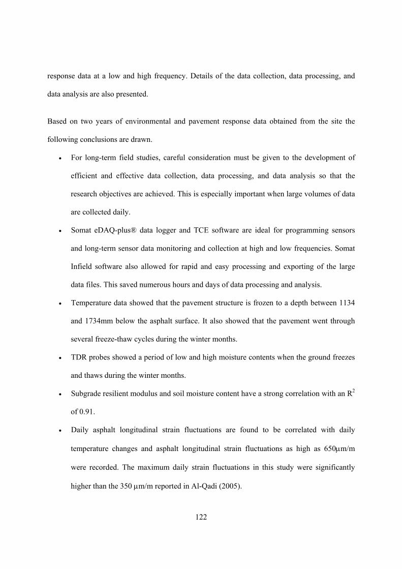
122

response data at a low and high frequency. Details of the data collection, data processing, and

data analysis are also presented.

Based on two years of environmental and pavement response data obtained from the site the

following conclusions are drawn.

For long-term field studies, careful consideration must be given to the development of

efficient and effective data collection, data processing, and data analysis so that the

research objectives are achieved. This is especially important when large volumes of data

are collected daily.

Somat eDAQ-plus® data logger and TCE software are ideal for programming sensors

and long-term sensor data monitoring and collection at high and low frequencies. Somat

Infield software also allowed for rapid and easy processing and exporting of the large

data files. This saved numerous hours and days of data processing and analysis.

Temperature data showed that the pavement structure is frozen to a depth between 1134

and 1734mm below the asphalt surface. It also showed that the pavement went through

several freeze-thaw cycles during the winter months.

TDR probes showed a period of low and high moisture contents when the ground freezes

and thaws during the winter months.

Subgrade resilient modulus and soil moisture content have a strong correlation with an R2

of 0.91.

Daily asphalt longitudinal strain fluctuations are found to be correlated with daily

temperature changes and asphalt longitudinal strain fluctuations as high as 650m/m

were recorded. The maximum daily strain fluctuations in this study were significantly

higher than the 350 m/m reported in Al-Qadi (2005).

123

6.8 Acknowledgement The authors acknowledge the Natural Sciences and Engineering Research Council of Canada






instrumentation.

124

Chapter 7: Observed Seasonal Variation of Environmental Factors and Their Impact on Flexible Pavement Performance Subject to Annual Freeze/ Thaw

7 Observed Seasonal Variation of Environmental Factors and Their Impact on Flexible Pavement Performance Subject to Annual Freeze/ Thaw

125

7.1 Overview This paper presents the results obtained over two years of field monitoring of environmental

parameters and pavement performance using a state-of-the-art field monitoring system installed

in the Center for Pavement and Transportation Technology (CPATT) test track located in

Waterloo, Ontario, Canada. The objective of the study was to quantify the seasonal variation of

environmental factors and pavement performance in a climate subject to freeze/thaw events. Site

data collected included soil moisture content, pavement temperature, Falling Weight

Deflectometer (FWD) subgrade resilient modulus, and meteorological data (rainfall and air

temperature). Soil moisture content and subgrade resilient modulus changes in the pavement

structure can be divided into three distinct Seasonal Zones. Seasonal Zone I consists of a

decreasing soil moisture content trend, Seasonal Zone II consists of an increasing soil moisture

trend, and Seasonal Zone III consists of frozen ground conditions.

126

7.2 Introduction Transportation agencies are currently considering the implementation of Mechanistic-Empirical

(M-E) method for pavement design. This methodology requires input of traffic and

environmental data to predict the pavement response and performance (NCHRP 2004) .

The M-E Design Guide uses an Enhanced Integrated Climatic Model (EICM) to estimate

unbound material resilient modulus. The EICM model records user-supplied resilient modulus

for all unbound layer materials at an initial or reference condition. Using climatic data, the EICM

evaluates changes in moisture content from an initial or a reference condition. Changes in soil

moisture content are then used to modify the initial user-supplied resilient modulus. It also

considers the effects of freezing, thawing and recovery on the reference resilient modulus. The

M-E design method uses changes in subgrade resilient modulus over time to predict pavement

response parameters and damage at various points within the pavement system.

Long-term field monitoring programs have been used to investigate seasonal variations of

environmental parameters and their effects on pavement response and performance (Salem 2004;

Zuo 2003). To date field studies have been completed in relatively mild climatic conditions

(Watson and Rajapakse 2000). Limited published environmental data exists for pavements

subject to seasonal freeze-thaw events, typical of the southern Canadian climatic conditions, to

validate or calibrate the M-E design method.

In this study, environmental factors and pavement performance were monitored over a two- year

period using a state-of-the-art field monitoring system installed at the Centre for Pavement and

Transportation Technology (CPATT) test track located in Waterloo, Ontario, Canada. Site data

collected included soil moisture content, pavement temperature, Falling Weight Deflectometer

127

(FWD) subgrade resilient modulus, and meteorological data (rainfall and air temperature). The

goal of this study was to quantify the seasonal variation of environmental factors and pavement

performance in a climate subject to freeze/ thaw events. This will be accomplished by (1)

investigating seasonal changes in soil moisture content and pavement temperature; (2)

determining correlations between meteorological data and measured changes in environmental

factors; and (3) evaluating pavement performance due to changes in environmental factors. The

use of the presented data for evaluation of M-E design approach will also be discussed.

7.3 CPATT Test Track In this study, environmental parameters and flexible pavement field response was measured at

the CPATT test track (709m long and eight meters wide) located in Waterloo, Ontario, Canada.

The instrumented test track section consists of 223 mm of Hot-Laid 3 (HL3) mix, consisting of

40 percent crushed gravel, 45% asphalt sand, 15% screenings, and 5.3% PG 58-28 asphalt

cement. Below the HL3 are 200mm of Granular A base aggregate and 300mm of Granular B

subbase aggregate. Compacted Granular A, 900mm in depth, is located below the subbase

aggregate. Below the compacted Granular A is site subgrade that consists of compacted fill and

well compacted clayey silt with some gravel. Granular A, as defined in the Ontario Provincial

Standard Specification (OPSS) 1010, consists of crushed rock composed of hard, uncoated,

fractured fragments, reduced from rock formations or boulders of uniform quality while Granular

B consists of clean, hard, durable uncoated particles from deposits of gravel or sand (MTO

2003).

128

Based on historical weather data from the University of Waterloo weather station, the average

monthly temperature at the site typically varies from -10°C during the winter months to 26 °C

during the summer months.

7.4 Data Collection System This section provides details on the state-of-the-art field instrumentation system implemented at

CPATT test track, meteorological data collected from the University of Waterloo weather

station, and FWD pavement surveys performed at the instrumented section.

7.4.1 Pavement Instrumentation A state-of-the-art field instrumentation system was developed and installed to measure

temperature of the asphalt, base, and subgrade materials, and soil moisture content in the

granular base and subgrade materials. Pavement temperatures were measured and recorded using

a Campbell CRX10 data logger with four Campbell Scientific T107B thermistors (T-1 to T-4)

installed 223, 530, 1134, and 1734mm below the asphalt surface respectively. Soil moisture was

measured and recorded using two Campbell Scientific CS616 Time Domain Reflectometer

probes (TDR 1 and TDR 2) installed 800 and 1150mm below the asphalt surface respectively

connected to Campbell CRX10 data logger. Figure 7-1 shows the distribution of the thermistors

and the TDR probes in the instrumented section. Probe data was collected at a rate of 1 reading

every 5 minutes (0.0033Hz). This sampling rate was deemed sufficient to record daily changes in

probe readings.

129

Figure 7-1: Pavement Profile and Sensors Location

Power was supplied to the data logger and probes using two 12V deep cycle batteries that were

recharged using a solar panel. To conserve battery power during the winter time - when the

duration of solar recharge was limited - a programmable timer was used to automatically turn the

system off and on at predefined intervals. A power regulator was also used to prevent batteries

from overcharging and discharging, and to prevent power flow from the batteries to the solar

panel.

Campbell Scientific CRX10, TDR, and thermistors data files (.DAT) were imported into a data

base consisting of 210,240 data points.

Further details about the field monitoring program can be found in Adedapo (2007).

130

7.4.2 Meteorological Data For this study precipitation and air temperature data were obtained from the University of

Waterloo weather station, located approximately five kilometers North East of the instrumented

test site. Data obtained from this weather station was deemed to be representative of the

conditions at the instrumented test site.

7.4.3 Pavement Performance Surveys FWD pavement surveys were performed on the instrumented test section by Applied Research

Associate Inc. to record changes in pavement performance during the two year monitoring

period. Test results provided by Applied Research Associate Inc. include pavement deflection

and the back-calculated subgrade resilient modulus.

7.5 Moisture Content Variation during Monitoring Period Figure 7-2 shows TDR1 (upper) and TDR2 (lower) moisture content changes from March 2004

to February 2006. The data gap in March 2005 corresponds to a period of 13 days when the data

logger was removed from the site. Figure 7-2 illustrates that the two TDR probes showed similar

response during the 2004-2005 and 2005-2006 monitoring period. The trends observed during

the monitoring period are noted below:

The March to April period has the highest recorded soil moisture content.

The April to October period has a decreasing trend in soil moisture content

The October to November/December period has an increasing trend in soil moisture

content.

131

The November to February period (winter months) has rapid and sudden fluctuations in

soil moisture content

0

5

10

15

20

25

30

Jan Feb Mar Apr May Jun Jul Aug Sep Oct Nov Dec Jan Feb Mar Apr May Jun Jul Aug Sep Oct Nov Dec Jan Feb

Monitoring Period

Soil

Mois

ture

Conte

net (%

)

2004 2005

TDR2 TDR2

TDR1TDR1

Figure 7-2 : 2004-2005 TDR1 Moisture Content

7.6 Pavement Temperature Variation over Monitoring Period Figure 7-3 shows pavement temperatures probes T-1, T-2, T-3 and T-4 variation from April 2004

to May 2005. This figure shows that all the temperature probes have a sinusoidal response. It

also shows that the daily and seasonal pavement temperature fluctuation decreases with depth

below the asphalt surface. For example, temperature probe T-1, located 22.3cm below the

asphalt layer, recorded a seasonal temperature variation of 38°C with daily temperature

fluctuations in the order of 10 to 20°C, while T-4 showed a seasonal temperature variation of 17

°C with daily temperature fluctuations in the order of 1°C.

132

-10

-5

0

5

10

15

20

25

30

Apr-04 May-04 Jun-04 Jul-04 Aug-04 Aug-04 Sep-04 Oct-04 Nov-04 Dec-04 Jan-05 Feb-05 Mar-05 Apr-05 May-05

Monitoring Period

Gro

un

d T

emp

era

ture

(oC

)

T-2

T-4

T-3

T-1

Figure 7-3: Temperature Variation at T-1, T-2, T-3, and T-4

Thermistor T-1, located 223 mm below the asphalt surface, indicates that freezing ground

conditions (temperature below 0oC) occur from November 2004 to the end of March 2005.

Thermistors T-2 and T-3, located 530 and 1134mm below the asphalt surface, indicate that

freezing ground conditions occur from December 2004/January 2005 to the end of March 2005.

Thermistor T-4, located 1734mm below the asphalt surface, indicates that no freezing ground

conditions occur over the monitoring period. For the site, the freezing depth is between 1134 and

1734mm below the asphalt surface. This correlates with the findings of the Ontario Ministry of

Transportation and Communications (now Ontario Ministry of Transportation) which initiated a

five year program aimed at measuring frost penetration in different subgrade soils throughout

133

Ontario. The depth of frost measured on Highway 7 in Guelph, Ontario, Canada between 1970

and 1975 ranged between 1.22m and 1.57m (Chisholm and Phang 1983).

The Guelph site is the closest instrumented site to the CPATT test facility. The CPATT

measured frost penetration depth is in agreement with the frost depth reported in the Ontario

Ministry of Transportation and Communications study.

7.6.1 Average Monthly Temperature Distribution Average monthly changes in pavement temperature from April 2004 to March 2005 are plotted

in Figure 7-4 and Figure 7-5. The temperature at depth zero is the average monthly air

temperature while the thermistor temperatures (T-1 to T-4) are from below the asphalt surface.

Figure 7-4 and Figure 7-5 show that the average monthly temperature at the base of the asphalt

(T-1) is always greater than the average monthly air temperature. From April to September 2004

(Figure 7-4), the base and subbase temperature generally decreases linearly with depth at

approximately 0.037C/cm. From October 2004 to March 2005 (Figure 7-5), the base and

subbase temperature generally increases linearly with depth at approximately 0.035C/cm.

Figure 7-5 shows that the pavement temperature, up to a depth of 120 cm, was at or below zero

degree Celsius from December 2004 to March 2005.

134

Figure 7-4: Monthly Temperature Distributions at Different Depth below Asphalt

Surface – April to September

Figure 7-5: Monthly Temperature Distributions at Different Depth below Asphalt –

October to March

135

7.7 Seasonal Zones Soil moisture changes were subdivided into three Seasonal Zones shown in Figure 7-6.

16

18

20

22

24

26

Apr-04 May-04 Jun-04 Jul-04 Aug-04 Sep-04 Oct-04 Nov-04 Dec-04 Jan-05 Feb-05 Mar-05 Apr-05

Monitoring Period

Soil M

ois

ture

Conte

nt (%

)

-10

-5

0

5

10

15

20

25

30

35

40

Averag

e Mon

thly

Tem

peratu

re ( oC

)

Zone I (Spring) Zone II (Fall) Zone III (Winter)

T-2

TDR2

Air Temperature

Figure 7-6: Moisture Content Zones for TDR2

Seasonal Zone I occurs during the spring and summer seasons when the soil moisture content

shows a decreasing trend. In Figure 7-6 Seasonal Zone I occurs from April to October 2004

when the soil moisture content decreases from approximately 25 to 21 percent. The decreasing

moisture content trend is inferred to be due to evaporation. Soil moisture content along with

rainfall precipitation from April 18 to May 28, 2004 is shown in Figure 7-7. This figure indicates

that temporary increases in soil moisture content occur with each significant precipitation event.

136

0

5

10

15

20

25

15-Apr 20-Apr 25-Apr 30-Apr 5-May 10-May 15-May 20-May 25-May 30-May

Monitoring Period

Rain

fall (

mm

)

22.5

23

23.5

24

24.5

25S

oil M

ois

ture

Co

nte

nt (%

)

TDR2

Rainfall

Figure 7-7: Rainfall Local Effect on Moisture Content Variation- Zone I

Seasonal Zone II occurs during the fall season when the soil moisture content shows an

increasing trend. In Figure 7-6 Seasonal Zone II occurs from October to December 2004 when

the soil moisture content increases from approximately 21 to 22 percent. In Seasonal Zone II the

average monthly air and ground temperature show a decreasing trend. At the end of this period

the average monthly air temperature is -4C and the average monthly T-2 ground temperature is

0C. Thus, the end of Seasonal Zone II and the beginning of Seasonal Zone III represent the

onset of freezing ground temperatures.

Seasonal Zone III is defined as the period during which freezing ground conditions occur. In

Figure 7-6 Seasonal Zone III occurs from December 2004 to March 2005. The soil moisture

content in Seasonal Zone III initially decreased rapidly from 22 to 18 percent. This is followed

137

by rapid soil moisture content fluctuations and then by a period in which the moisture content is

relatively constant (18.3 percent). Soil moisture content along with T-2 ground temperature from

April 18 to May 28, 2004 is shown in Figure 7-8.

18

19

20

21

22

23

24

Oct-04 Nov-04 Dec-04 Jan-05 Feb-05 Mar-05

Monitoring Period

Soil

Mois

ture

Conte

nt (%

)

-10

-5

0

5

10

15

Gro

und T

em

pera

ture

( oC)

TDR2

T-2

Zone II (Fall) Zone III (Winter)

Figure 7-8: Temperature Correlation with Moisture Content (Zone II & III)

This figure shows that a rapid decrease in soil moisture content occurs when the temperature

goes below zero degrees Celsius and rapid increases in soil moisture occur when the ground

temperature is above zero degrees Celsius. Patterson and Smith (1981) found through laboratory

testing of frozen soils that TDR probes provide an indication of unfrozen pore water since the

dielectric constant of ice is similar to that of dry soil. Thus, it can be inferred that when the

ground freezes the TDR probe will show a rapid decrease in soil moisture content and a rapid

increase in soil moisture content when the ground thaws. The TDR rapid response is due to the

changes in the volume of unfrozen pore water.

138

7.8 Moisture and Pavement Performance Variation over Monitoring Period

Subgrade resilient modulus, back-calculated from FWD data performed in the vicinity of the

instrumented section, along with TDR1 soil moisture content from April 2004 to February 2005

are shown in Figure 7-9.

Figure 7-9: Correlation of FWD Deflection with Subgrade Resilient Modulus

This figure shows that the resilient modulus and moisture content are inversely correlated. For

this site, a non-liner regression correlation, with a R2 of 0.91, was found to fit the data.

0694.0.17.211 eM R

( 7-1)

139

where MR is the subgrade resilient modulus (MPa), e is natural logarithm, and is soil moisture

content in percentage.

Equation 7-1 and TDR 1 soil moisture content was used to predict the subgrade resilient modulus

for the monitoring period shown in Figure 7-9. Predicted and FWD resilient modulus indicate

that subgrade resilient modulus increases linearly in Seasonal Zone I, decreases linearly in

Seasonal Zone II, and fluctuates dramatically during freeze-thaw events in Seasonal Zone III.

The lowest subgrade resilient modulus (15 MPa) occurs at the beginning of Seasonal Zone I -

2005 when the ground rebounds from freezing. The highest subgrade resilient modulus (50 MPa)

occurs when the ground is frozen. The highest unfrozen subgrade resilient modulus (34 MPa)

occurs at the end of Seasonal Zone I-2004. The subgrade resilient modulus MR at any time can be

expressed using Equation 7-2 (NCHRP 2004):

RoptENVR MFM

( 7-2)

where FENV is an adjustment factor and MRopt is the subgrade resilient modulus at optimum

condition.

Using the highest unfrozen subgrade resilient modulus as MRopt, FENV were determined for each

Seasonal Zone and are presented in Table 7-1.

140

Table 7-1: Maximum and Minimum FENV for Each Seasonal Zone

Fenv

Seasonal ZoneMax Min

I-2004 1.0 0.6

II-2004 1.0 0.8

III-2004 1.5 0.6

I-2005 0.7 0.5

Table 7-1 indicates that the environmental adjustment factor increases in Seasonal Zone I from

0.5 to 1.0, decreases in Seasonal Zone II from 1.0 to 0.8, and fluctuates between 0.6 to 1.5 in

Seasonal Zone III.

The environmental adjustment factor can be compared with the seasonal factors developed in

Alberta, which is considered a seasonal frost area, and shown in Table 7-2 . This study was

conducted in 1989 to 1994 by Alberta Transportation and Utilities to investigate the seasonal

variation of subgrade strength (AT and U. 1997). FWD tests were performed on several

pavement sections and the subgrade resilient modulus was back-calculated using the ELMOD

computer program.

141

Table 7-2: Seasonal Factors in Alberta

Month Jan Feb Mar Apr May Jun Jul Aug Sep Oct Nov Dec

Seasonal Factor 5.00 5.00 2.75 0.63 0.88 1.00 1.00 1.00 1.00 1.00 2.00 4.00

7.9 Summary and Conclusions This paper presented and discussed soil moisture and ground temperature data, recorded at five

minute intervals over a two year monitoring period at the CPATT test track facility, located in

Waterloo, Ontario, Canada. Rainfall precipitation, air temperature and FWD data were also

presented and discussed.

Based on the data and information presented the following conclusions are drawn.

1. Soil moisture content and subgrade resilient modulus changes in the pavement structure

can be divided into three distinct Seasonal Zones. Zone I consists of a period of

decreasing soil moisture that occurs during the summer months, Zone II consists of a

period of increasing soil moisture that occurs during the fall season, and Zone III consists

of a period of low and high moisture contents when the ground freezes and thaws during

the winter months.

2. In Zone I only significant rainfall event appeared to create a short-term and temporary

increase in soil moisture. During the winter month the ground froze to a depth of at least

120cm.

142

3. Seasonal Zones can be used to estimate changes in resilient subgrade modulus for

pavement response predictions. Although EICM provides environmental data on an

hourly basis, it is obviously impractical to perform the linear elastic or the finite element

analysis on an hourly basis. Therefore, the less number of analyses can be performed

using the similarities inside each Seasonal Zone.

4. The EICM model in the M-E Deign method predicts changes in soil moisture content

over time using climatic data. Currently, the climatic data required to input into the EICM

model is not available for the CPATT test track site. Should climatic data for the site

become available, EICM predications can be validated and/or calibrated for southern

Ontario conditions using the above noted field data.

7.10 Acknowledgement The authors would like to thank Professor Ralph Hass for his support during this research.

Thanks are also for Natural Science and Engineering Research Council of Canada (NSERC) and

CPATT due to funding this research project. Thanks are also due to Asphalt Research Associate

Inc. (ARA) help in providing FWD data. The authors also appreciate Ken Bowman and Terry

Ridgway, University of Waterloo technical staf, for their contribution during instrumentation and

data collection.

143

Chapter 8: Measurement and Analysis of Flexible Pavement Thermal-Induced Strains

8 Measurement and Analysis of Flexible Pavement Thermal-Induced Strains

144

8.1 Overview The focus of this study was to quantify the asphalt strain amplitude that occurs in flexible

pavements as a result of thermal loading. A state-of-the-art field monitoring program was

developed at the Centre for Pavement and Transportation Technology (CPATT) test facility to

measure flexible pavement response to thermal loads. Asphalt temperature and longitudinal

strain collected over a two years monitoring program were analyzed to interpret pavement

response to thermal loads. Daily strain fluctuations as high as 650m/m, and the irrecoverable

strain as high as 2500m/m per year were observed during 2004-2005 and 2005-2006.

145

8.2 Introduction The trend to move toward a more mechanistic approach in flexible pavement design has

emphasized the need to more accurately characterize pavement response and performance to

environmental factors and vehicle loads. Temperature, one of the main environmental factors,

affects the performance of the pavement materials (Mahoney and Vinson 1983). Low-

temperature cracking and thermal fatigue cracking are two major distresses in flexible pavement

as a result of thermal loads (Vinson et al. 1989).

Low-temperature cracking is a serious distress found in asphalt pavements that manifests itself

through a uniform, often equally spaced, pattern of cracks perpendicular to the direction of traffic

(Jackson and Vinson 1996; Shen and Kirkner 1999; Timm et al. 2003; Vinson et al. 1989;

Zubeck and Vinson 1996). As the temperature drops the restrained pavement tries to contract and

the tensile stress increases until it exceeds the tensile strength of Hot Mix Asphalt (HMA) and

pavement cracks (Vinson et al. 1989). The current Superpave binder specification specifies a

limiting low temperature for the asphalt binder to limit the occurrence of low-temperature

cracking.

Unlike the low-temperature cracking, thermal fatigue cracking does not require a very low level

of temperature to occur (Al-Qadi et al. 2005; Vinson et al. 1989). Similar to load-associated

fatigue cracking, thermal fatigue cracking is the result of repetitive thermal cycles that cause

cyclic stresses and strains in the material and a buildup of irrecoverable deformations (Al-Qadi et

al. 2005).

146

Although significant advancements have been achieved in understanding the mechanisms of

thermal fatigue cracking, there have not been enough field measurements that address the

criticality of the associated strain amplitude in real pavements (Al-Qadi et al. 2005). Al-Qadi et

al. (2005) carried out a field experimental program to measure thermal-induced strain in Virginia

Smart Road. The result of the study indicates that the pavement response to thermal loading was

associated with a high strain range, reaching a maximum recorded value of 350μm/m. The study

confirms that unlike the wheel load- associated fatigue cracking, the criticality of thermal fatigue

arises from the high stress-strain level exhibited in each cycle rather than its frequency. To date,

no measurements have been performed to investigate the criticality of thermal-induced strains for

pavements subjected to climates with freeze-thaw cycles (such as southern Canada).

A field investigation program was developed at the University of Waterloo to investigate the

measured thermal-induced strain associated with thermal fatigue cracking in a climate subjected

to freeze-thaw cycles. This paper provides an overview of the Centre for Pavement and

Transportation Technology (CPATT) field test facility and presents the findings from a two year

monitoring period.

8.3 CPATT Field Test Facility

8.3.1 Site Information In this study, pavement temperature and asphalt longitudinal strain were measured at the CPATT

test track (709m long and eight meters wide) located in Waterloo, Ontario, Canada. The

instrumented test track section consists of 223 and 185mm of Hot-Laid 3 (HL3) mix, consisting

of 40 percent crushed gravel, 45% asphalt sand, 15% screenings, and 5.3% PG 58-28 asphalt

147

cement, on west and east lane respectively. Below the HL3 are 200mm of Granular A base




defined in the Ontario Provincial Standard Specification (OPSS) 1010, consists of crushed rock

composed of hard, uncoated, fractured fragments, reduced from rock formations or boulders of


deposits of gravel or sand (MTO 2003).

Based on historical weather data from the University of Waterloo weather station, the site

average monthly mean air temperature typically varies from -10°C during the winter months to

26 °C during the summer months. Further details about the test track facility including its

construction and pavement performance, can be found in Tighe et al. (2003).

8.3.2 Instrumentation A state-of-the-art field instrumentation system was developed and installed to measure

temperature of the asphalt, base, and subgrade materials, and asphalt longitudinal strain.

Pavement temperatures were measured and recorded using a Campbell CRX10 data logger with

four Campbell Scientific T107B thermistors (T-1 to T-4) installed 223, 800, 1350, and 1950mm

below the asphalt surface respectively (Figure 8-1). Asphalt longitudinal strain was measured

and recorded using five ASG-152 H-type asphalt strain gauges. As shown in Figure 8-1, ASG3

was placed on the road centerline, while ASG1 and ASG2 were placed 690 and 2700mm from

the west pavement edge respectively. ASG5 and ASG 4 were placed 1380 and 3200mm from

148

the east pavement edge respectively. Asphalt strain gauge data was collected using a Somat

eDAQ-plus®, data logger with the sampling rate set at 0.01 Hz (1 reading every 1.67 minutes).


Thermistor and asphalt strain gauge data was collected at a rate of 1 reading every 5 minutes

(0.0033Hz). This sampling rate was deemed sufficient to record daily changes in probe readings.

Power was supplied to the data logger and probes using two 12V deep cycle batteries that were

recharged using a solar panel. To conserve battery power during the winter time - when the

duration of solar recharge was limited - a programmable timer was used to automatically turn the

system off and on at predefined intervals. A power regulator was also used to prevent batteries

from overcharging and discharging, and to prevent power flow from the batteries to the solar

panel. Further details about the field monitoring program can be found in Adedapo (2007).

8.3.3 Thermal-Induced Strain-2004 Figure 8-2 shows the measured asphalt longitudinal strain (ASG5) at the bottom of the asphalt

layer and the ambient air temperature for forty days period from August 21 to October 10, 2004.

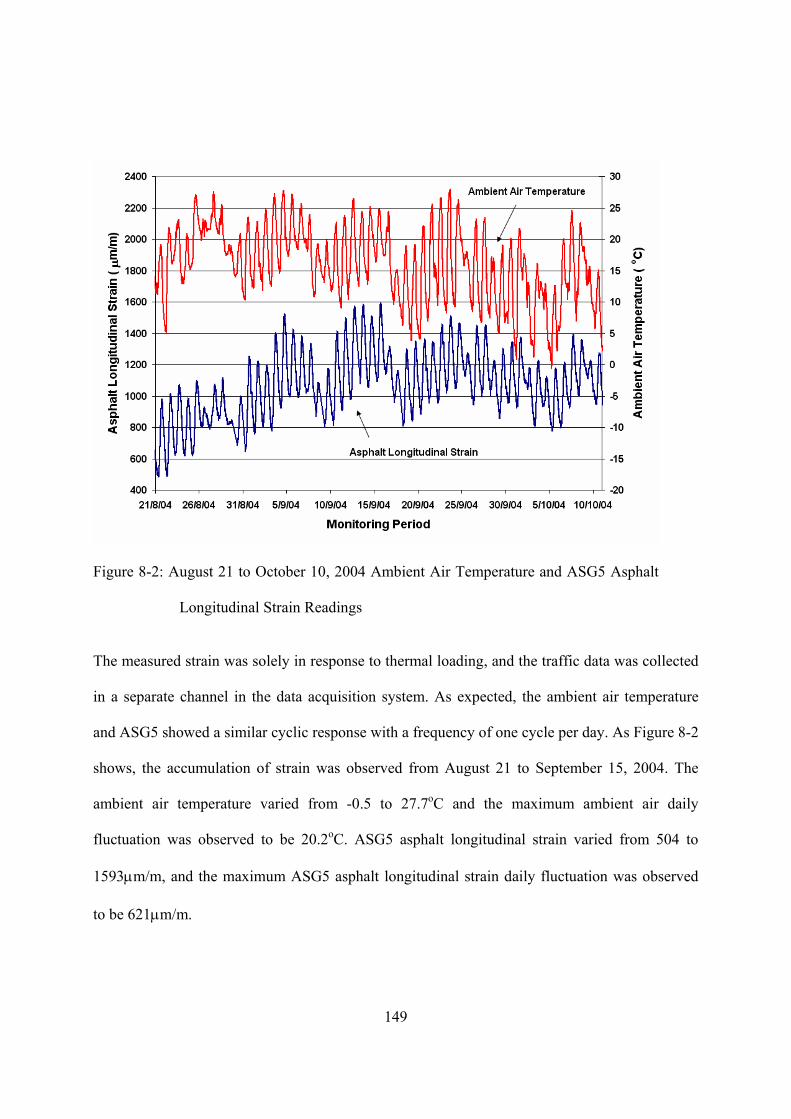
149


Longitudinal Strain Readings

The measured strain was solely in response to thermal loading, and the traffic data was collected

in a separate channel in the data acquisition system. As expected, the ambient air temperature

and ASG5 showed a similar cyclic response with a frequency of one cycle per day. As Figure 8-2

shows, the accumulation of strain was observed from August 21 to September 15, 2004. The

ambient air temperature varied from -0.5 to 27.7oC and the maximum ambient air daily

fluctuation was observed to be 20.2oC. ASG5 asphalt longitudinal strain varied from 504 to

1593m/m, and the maximum ASG5 asphalt longitudinal strain daily fluctuation was observed

to be 621m/m.

150

Figure 8-3 shows the temperature at the bottom of the asphalt layer (T-1) and the measured

asphalt longitudinal strain (ASG5) for the same monitoring period shown in Figure 8-2. Similar

to ambient air, T-1 showed the cyclic response that varied from 12.1 to 27.8 oC. The maximum

T-1 daily fluctuation was observed to be 5.96 oC.

Figure 8-3: August 21 to October 10, 2004 Temperature below the Asphalt (T-1) and

ASG5 Asphalt Longitudinal Strain Readings

Similar cyclic behavior was observed in the other asphalt strain gauges. Figure 8-4 shows the

ASG3 asphalt longitudinal strain and the ambient air temperature for the same monitoring period

shown in Figure 8-2. ASG3 asphalt longitudinal strain varied from 574 to 1685m/m. The

maximum ASG3 daily strain fluctuation was observed to be 610m/m.

151



8.3.4 Daily Thermal-Induced Strain Fluctuation The daily thermal-induced strain fluctuation was calculated using Equation 8-1 (Norman 1999):

minmax

( 8-1)

where:

=Daily Thermal-Induced Asphalt Longitudinal Strain Fluctuation (m/m)

max

=Daily Maximum Asphalt Longitudinal Strain (m/m)

152

min =Daily Minimum Asphalt Longitudinal Strain (m/m)

Figure 8-5 shows the measured ASG5 daily thermal-induced strain fluctuation from January

2004 to January 2005. All strain gauges showed a similar trend.

Figure 8-5: 2004 Thermal-Induced ASG5 Asphalt Longitudinal Strain Fluctuations

Small gaps at the measurements correspond to the periods when the data logger was inactive in

the site. Figure 8-5 shows that daily strain fluctuation between 600 and 650m/m can occur due

to daily temperature changes.

Figure 8-6 shows the average ASG5 daily thermal-induced strain fluctuation from January to

December 2004 and the average temperature fluctuation below the asphalt layer (T-1) from May

to December 2004. The temperature data was not available from January to April 2004.

153

Figure 8-6: 2004 Average T-1 Temperature Fluctuations and Average ASG5 Daily

Thermal-Induced Asphalt Longitudinal Strain Fluctuations

Figure 8-6 shows that the higher strain fluctuation occurs from May to September (spring and

summer). It is evident from Figure 8-6 that the average daily strain fluctuation correlates to the

average temperature fluctuation below the asphalt layer.

8.3.5 Thermal-Induced Strain and Temperature below the Asphalt The least squared regression method was used to study the correlation between the ASG5 daily

strain fluctuation and the temperature fluctuation below the asphalt layer. A linear relationship

was found to fit the data with R2 of 0.91 (Figure 8-7).

154

Figure 8-7: 2004 Daily ASG5 Thermal-Induced Asphalt Longitudinal Strain

Fluctuations versus T-1 Temperature Fluctuation below the Asphalt Layer

8.3.6 Thermal Induced Strain- 2005 Figure 8-8 shows the measured ASG5 asphalt longitudinal strain and ambient air temperature

from September 10-25, 2005. During this period, the ambient air temperature varied from 6 to

30oC, while the measured asphalt longitudinal strain level varied from 2059 to 3051m/m.

155

Figure 8-8: September 10 to 24, 2004 Ambient Air Temperature and ASG5 Asphalt


It is evident from Figure 8-8 that the strain level in September 2005 (2059 to 3051m/m)

increased compared to the measurements shown in Figure 8-2 from September 2004 (850 to

1593m/m). Similar increases in strain were observed in the other strain gauges.

8.3.7 2004-2006 Asphalt Strain Gauge Figure 8-9 shows the measured ASG5 asphalt longitudinal strain, T-1 temperature below the

asphalt layer, and the ambient air temperature for the monitoring period of 2004-2006. Small

gaps in the measurements correspond to the periods when the data logger was inactive at the site.

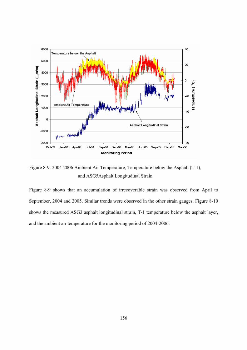
156

Figure 8-9: 2004-2006 Ambient Air Temperature, Temperature below the Asphalt (T-1),

and ASG5Asphalt Longitudinal Strain

Figure 8-9 shows that an accumulation of irrecoverable strain was observed from April to

September, 2004 and 2005. Similar trends were observed in the other strain gauges. Figure 8-10

shows the measured ASG3 asphalt longitudinal strain, T-1 temperature below the asphalt layer,

and the ambient air temperature for the monitoring period of 2004-2006.

157


ASG3 Asphalt Longitudinal Strain

Using the ASG5 strain measurements, shown in Figure 8-9, the average monthly asphalt

longitudinal strain level was calculated for 2004-2005 and 2005-2006 (Figure 8-11 and Figure

8-12).

158

Figure 8-11: 2004-2005 Average Monthly ASG5 Longitudinal Strain Level

Figure 8-12: 2005-2006 Average Monthly ASG5 Longitudinal Strain Level

159

The 2004-2005 strain level fluctuation was observed to be 2544m/m comprising of 206m/m

recoverable and 2338m/m irrecoverable. The 2005-2006 strain level fluctuation was observed

to be 1684m/m comprising of 645m/m recoverable and 1039m/m irrecoverable.

8.4 Summary and Conclusions The objective of this study was to quantify the asphalt strain amplitude associated with thermal

loading in flexible pavements. A state-of-the-art field monitoring program was implemented to

measure temperature of the asphalt, base, and subgrade materials, and asphalt longitudinal strain.

Results of the experimental program indicate that pavement response to thermal loading is

associated with a very high strain range with a maximum recorded value of 680m/m. The

accumulation of irrecoverable strain was observed during spring and summer during both the

monitoring years. The irrecoverable strain was 2338m/m during 2004-2005 and 1039m/m

during 2005-2006. The results strongly suggest that the strain associated with thermal loads are

extremely critical for accurate pavement performance prediction.

160

8.5 Acknowledgements The authors acknowledge the Natural Sciences and Engineering Research Council of Canada






instrumentation.

161

Chapter 9: Conclusions and Recommendations

9 Conclusions and Recommendations

162

9.1 General Summary The focus of this study was to investigate the impact of traffic loads and environmental

conditions at the CPATT test facility in Waterloo, Ontario, Canada. Pavement responses were

measured under a variety of wheel loads by utilizing a state-of-the-art field instrumentation and

data acquisition system. A detailed controlled wheel load test was performed to verify pavement

responses under a variety of traffic loading and environmental conditions. A three-step procedure

was implemented to identify the dynamic modulus of the HL3 material. A finite element model

was developed using MichPave program to predict the asphalt longitudinal strain for a variety of

loading conditions. The predicted responses were compared to the measured field responses. The

daily and seasonal changes in environmental parameters that affect flexible pavement response

and performance was monitored and measured using the instrumentation system. FWD and

direct strain measurement were used to quantify the impact of environmental parameters on

pavement response and performance.

A number of contributions to the understanding of the influence of traffic and environmental

loads on flexible pavement response and performance have been presented in this dissertation.

The conclusions from the various investigations are provided at the end of each chapter Key

findings of this research are summarized and presented below. Suggestions for further work are

also provided.

163

9.2 Conclusions

CPATT Field data is a unique and represents response of flexible pavements under

freeze/thaw environments.

The CPATT instrumentation system, which includes remote access and control

capabilities, has worked exceptionally well for over six years. The remote monitoring

system provides real-time access to the instrumentation system that reduces required site

visits, ensures continuous data collection, and enables to detect any form of abnormalities

within the instrumentation system.

Two data acquisition systems were implemented at the CPATT test facility. Low

frequency data acquisition system is used to record daily temperature and soil moisture

content changes and high frequency to record pavement stresses and strains due to

passing wheel loads.

A detailed wheel controlled test was performed to determine the impacts of wheel

wander, vehicle speed, and changes in asphalt temperature on sensor readings. The

following findings were observed:

o Asphalt Longitudinal strain showed that the pavement fully recovers after each

wheel pass.

o Wheel wander was found to make significant change on asphalt longitudinal

strain. Wheel wander of 16 cm reduced asphalt longitudinal strains by 36 percent.

164

o An exponential relationship was found between asphalt longitudinal strains and

asphalt mid-depth temperature when the truck speed and wheel loading was

constant. The daily temperature fluctuations can double the asphalt longitudinal

strain.

o The measured asphalt longitudinal strain was found to decrease with increasing

truck speed.

o Using the stress pulse recorded at pressure cells, the loading time was found to be

a function of truck speed and depth below the pavement surface.

The laboratory determined dynamic modulus for HL3 was found to be:

o An exponential function of the test temperature when loading frequency was

constant.

o A non-linear function of the loading frequency when the test temperature was

constant.

The comparison of laboratory dynamic modulus and field measured asphalt longitudinal

strain showed that the laboratory determined dynamic modulus was inversely

proportional to the field measured asphalt longitudinal strain.

A simplified method was proposed to characterize HMA properties using the laboratory

dynamic modulus test, pressure cell data, and asphalt temperature. Pavement response

obtained with the field representative dynamic modulus correlated with field measured

asphalt longitudinal strains.

165

Two years of environmental monitoring showed that :

o For long-term field studies, when large volume of data are collected, careful

consideration must be given to the development of efficient and effective data

collection, processing, and analysis.

o Somat eDAQ-plus® data logger and TCE software were found to be ideal for

programming sensors and for long-term data collection at high and low

frequencies.

TDR probes and FWD data showed that Soil moisture content and subgrade resilient

modulus changes in the pavement structure can be divided into three distinct Seasonal

Zones. Zone I consists of a period of decreasing soil moisture that occurs during the

summer months, Zone II consists of a period of increasing soil moisture that occurs

during the fall season, and Zone III consists of a period of low and high moisture contents

when the ground freezes and thaws during the winter months.

Temperature data showed that during the winter months the ground froze to a depth

between 1134 and 1734mm below the asphalt surface. It also showed that the pavement

went through several freeze-thaw cycles during the winter months.

Daily asphalt longitudinal strain fluctuations were found to be correlated with daily

temperature changes with a maximum recorded value of 680m/m.

166

The cumulative irrecoverable pavement strains were observed during spring and summer

in both monitoring years. The irrecoverable strain was 2338m/m during 2004-2005 and

1039m/m during 2005-2006.

9.3 Recommendations and Future Work The trend to move toward M-E pavement design methods emphasizes the need to identify the

impact of traffic and environmental loads on pavement response and to develop realistic and

accurate models to compute and predict critical pavement responses. This study provided insight

into traffic and environmental parameters affecting pavement dynamic load responses. It also

validated the chosen model for asphalt longitudinal strain.

The following recommendations are suggested for future studies:

Although various conditions in finite element analyses and the material behavior of HMA

were considered and data from a multitude of controlled vehicle runs were examined,

exploration of other wheel load configurations and pavement sections are recommended

to expand the predictive capability of the proposed method.

Comparison of the field measured pavement response with prediction of other finite

element programs.

Validation of the proposed finite element model for vertical stresses at the top of base,

subbase, and subgrade.

Validation of the proposed finite element model for soil strain gauge data.

167

Numerical simulation of pavement subjected to temperature variation.

Evaluation of nonlinear elastic models for unbound granular materials

Continue monitoring environmental parameters and pavement performance to investigate

to establish seasonal shift factors that can reflect the variation of the temperature and

moisture content.

168

References

AASHO (1962). The AASHO Road Test., National Research Council, Washington, D.C., USA.

AASHTO. (1993). Guide for Design of Pavement Structures, American Association of State

Highway and Transportation Officials, Washington, D.C., USA.

AASHTO (2003). Standard Test Method for Determining Dynamic Modulus of Hot-Mix Asphalt

Concrete Mixtures., American Association of State Highway and Transportation Officials.

Acum, W. E. A., and Fox, L. (1951). "Computation of Load Stresses in a Three-Layer Elastic

System." Geotechnique, 2, 293-300.

Adedapo, A. A. (2007). Pavement Deterioration and PE Pipe Behavior Resulting from Open-Cut

and HDD Pipeline Installation Techniques., PhD Thesis, University of Waterloo, Ontario,

Canada.

Akhter, G. F., and Witczak, M. W. (1985). "Sensitivity of Flexible Pavement Performance to

Bituminous Mix Properties." Transp. Res. Rec., 70-79.

Al-Qadi, I. L., Loulizi, A., Elseifi, M., Lahouar, S. (2004). "The Virginia Smart Road: The

Impact of Pavement Instrumentation on Understanding Pavement Performance." Proc.,

Association of Asphalt Paving Technologist, White Bear Lake, MN, United States, 427-465.

Al-Qadi, I. L., Loulizi, A., Janajreh, I., Freeman, T. E. (2002). "Pavement Response to Dual

Tires and New Wide-Base Tires at Same Tire Pressure." Trans. Res. Rec., (1806), 38-47.

169

Al-Qadi, I. L., Hassan, M. M., Elseifi, M. A. (2005). "Field and Theoretical Evaluation of

Thermal Fatigue Cracking in Flexible Pavements." Trans. Res. Rec., 1919, 87-95.

AMADEUS. (2000). AMADEUS: Advanced Models for Analytical Design of European

Pavement Structures, Belgian Road Research Centre, Belgian.

AT and U. (1997). Pavement Design Manual., Alberta Infrastructure and Transportation, Edition

1.

Baker, H. B., Buth, M. R., Van Deusen, D. A. (1994). Minnesota Road Research Project: Load

Response Instrumentation Installation and Testing Procedures, Minnesota Dept. of

Transportation, Maplewood.

Bari, J., and Witczak, M. (2005). “Evaluation of the Effect of Lime Modification on the

Dynamic Modulus Stiffness of HMA: Use with the New RR 1929 M-E

Pavement Design Guide." Trans. Res. Rec., (1929), 10-19.

Boussinesq, J. (1885). Application Des Potentiels à l'Étude De l'Équilibre Et Du Mouvement Des

Solides Élastiques. Paris: Lille, 57–75.

Brown, E. R. (2006). NCAT Test Track Findings, Better Roads, 76(11), 82-87.

Burmister, D. M. (1945). "The General Theory of Stresses and Displacements in Layered Soil

Systems." Journal of Applied Physics, 16, Paris, France.

170

Chatti, K., Mahoney,P., Monismith, C. L., Tom, M.(1995). Field Response and Dynamic

lodeling of an Asphalt Concrete Pavement Section under Moving Heavy Trucks., University

of Michigan Transportation Research Institute, Ann Arbor, MI.

Chisholm, R. A., Phang, W. A. (1983). “Measurement and Prediction of Frost Penetration in

Highway”. Trans. Res. Rec., No 918, Washington D.C., 1-10.

Christison, J. T., Anderson, K. O., Shields, B. P. (1978). "In Situ Measurements of Strains and

Deflection in a Full-Depth Asphaltic Concrete Pavement.”, Proc., Assoaciation of Asphalt

Pavement Technologies, 47, Minneapolis, Minn., 398-433.

COST 333. (1997.) Development of New Bituminous Pavement Design Method., European

Commission, Office for Official Publications of the European Communities, Luxembourg.

Doré, G., and Duplain, G. (2002). “Monitoring Pavement Response during Spring Thaw using

Fiber-Optic Sensors24." Proc., 6th International Conference on the Bearing Capacity of

Roads and Airfields, Lisbon, Portugal.

Drumm, E. C., Reeves, J. S., Madgett, M. R., Trolinger, W. D. (1997). "Subgrade Resilient

Modulus Correction for Saturation Effects." J. Geotech. Geoenviron. Eng., 123(7), 663-670.

Elseifi, M. A., Al-Qadi, I. L., Yoo, P. J. (2006). “Viscoelastic Modeling and Field Validation of

Flexible Pavements." ASCE Journal of Engineering Mechanics, 132(2), 172-178.

Fernando, E. G., Musani, D., Park, D., Liu, W. (2006). Evaluation of Effects of Tire Size and

Inflation Pressure on Tire Contact Stresses and Pavement Response, Texas Transportation

Institute, Texas A&M University System, College Station, Texas.

171

Haas, R.C.G (1968). “Low Temperature Performance of Flexible Pavements" .Proc., Canadian

Technical Asphalt Association, Ottawa, Ontario, Canada.

Hadi, M., and Bodhinayake, B. C. (2003). “Non-Linear Finite Element Analysis of Flexible

Pavements.", Advances in Engineering Software, 34, 657-662.

Hamad, A. (2007). Effect of Axle Load and Seasonality on Thin Membrane Pavements., M.Sc

Thesis, University of Calgary, Canada.

Harichandran, R. S., Yeh, M. S., Baladi, G. Y. (1990). “MichPave: A Nonlinear Finite Element

Program for Analysis of Flexible Pavements." Trans. Res. Rec., (1286), 123-131.

Hildebrand, G. (2002). Verification of Flexible Pavement Response from a Field Test., Ph.D

Thesis, Cornell University, USA.

Huang, Y. H. (1993). Pavement Analysis and Design, Prentice Hall, Englewood Cliffs, New

Jersey, USA.

Huang, B., Mohammad, L. N., Rasoulian, M., Roberts, F. L., Qin, H. (2002). "

Numerical Validation of Pavement Performance at the Louisiana Accelerated Loading

Facility (ALF)." Proc., Ninth International Conference on Asphalt Pavements, Copenhagen,

Denmark.

Huhtala, M., Pihlajamaki, J., Pienimaki, M. (1989). “Effects of Tires and Tire Pressures on Road

Pavements.", Trans. Res. Rec., (1227), 107-114.

172

Immanuel, S., and Timm, D. H. (2006). "Measured and Theoretical Pressures in Base and

Subgrade Layers under Dynamic Truck Loading." Proc., 2006 Airfield and Highway

Pavement Specialty Conference, American Society of Civil Engineers, 155-166.

Jackson, N. M., and Vinson, T. S. (1996). "Analysis of Thermal Fatigue Distress of Asphalt

Concrete Pavements." Transp. Res. Rec., (1545), 43-49.

Knight, M. A., Tighe, S. T., Adedapo, A. (2004). "Trenchless Installation Preserves Pavement

Integrity." Proc., Annual Conference of the Transportation Association of Canada, Quebec

City.

Li, D., and Selig, E. T. (1994). "Resilient Modulus for Fine-Grained Subgrade Soils." J. Geotech.

Eng., 120(6), 939-957.

Liao, Y. (2007). Viscoelastic FE Modeling of Asphalt Pavements and its Application to U.S. 30

Perpetual Pavements, PhD Thesis, Ohio University.

Loulizi, A., Al-Qadi, I. L., Flintsch, G. W., Freeman, T. E. (2002). "Using Field Measured

Stresses and Strains to Quantify Flexible Pavement Responses to Loading." Proc., Ninth

International Conference on Asphalt Pavements, International Society for Asphalt

Pavements, Copenhagen, Denmark.

Loulizi, A., Al-Qadi, I. L., Lahouar, S., Freeman, T. E. (2001). "Data Collection and

Management of Instrumented Smart Road Flexible Pavement Sections." Transp. Res. Rec.,

(1769), 142-151.

173

Loulizi, A., Al-Qadi, I. L., Elseifi, M. (2006). "Difference between in Situ Flexible Pavement

Measured and Calculated Stresses and Strains." J. Transp. Eng., 132(7), 574-579.

Loulizi, A., Flintsch, G., Al-Qadi, I., Mokarem, D. (2006). "Comparing Resilient Modulus and

Dynamic Modulus of Hot-Mix Asphalt as Material Properties for Flexible Pavement

Design." Transp. Res. Rec., (1970), 161-170.

Loulizi, A., Al-Qadi, I., Lahouar, S., Freeman, T. E. (2002). "Measurement of Vertical

Compressive Stress Pulse in Flexible Pavements: Representation for Dynamic Loading

Tests." Transp. Res. Rec., (1816), 125-136.

Mahoney, J. P., and Vinson, T. S. (1983). “Mechanistic Approach to Pavement Design in Cold

Regions", Proc., Permafrost 4th International Conference, Washington, DC, USA, 779-782.

Mamlouk, M. S., and Mikhail, M. Y. (1998). “Concept for Mechanistic-Based Performance

Model for Flexible Pavements." Trans. Res. Rec., (1629), 149-158.

Metcalf, J. B. (1996). NCHRP Synthesis of Highway Practice 325: Application of Full-Scale

Accelerated Pavement Testing. Transportation Research Board, National Research Council,

Washington, D.C.

Monismith, C. L. (2004). “Evolution of Long Lasting Asphalt Design Methodology: A

Perspective", Distinguished Lecture, Proc., International Symposium on Design and

Construction of Long Lasting Asphalt Pavements, Auburn University, Alabama.

174

Monismith, C. L., Marker, V., Anderson, K. O., Shields, B. P., Dacyszyn, J. M., Schmidt, R. J.,

Zube, E., Kelly, J. E. (1966). "Symposium - Non-Traffic Load Associated Cracking of

Asphalt Pavements." Association of Asphalt Paving Technologists, 239-357.

MTO. (2003). Ontario Provincial Standard Specification for Aggregates-Base, Subbase, Select

Subgrade, and Backfill Material, Ministry of Transportation Ontario, Ontario, Canada.

NCHRP (2004). Guide for Mechanistic-Empirical Design of New and Rehabilitated Pavement

Structures, National Cooperative Highway Research Program.

Newmark, N. (1947). “Influence Charts for Computation of Vertical Displacements in Elastic

Foundations”, University of Illinois Experiment Station Bulletin, 367.

Norman, D. (1999). Mechanical Behavior of Materials: Engineering Methods for Deformation,

Fracture, and Fatigue, Prentice Hall, Upper Saddle River, N.J.

Park, D., Buch, N., Chatti, K. (2001). "Effective Layer Temperature Prediction Model and

Temperature Correction via Falling Weight Deflectometer Deflections." Transp. Res. Rec.,

1764, 97-111.

Park, H. M., Kim, Y. R., Park, S. W. (2005). “Assessment of Pavement Layer Condition with use

of Multiload-Level Falling Weight Deflectometer." Trans. Res. Rec., (1905), 107-116.

Patterson, D.E., Smith, M. W. (1981). ‘The Measurement of Unfrozen Water Content by the

Time Domain Reflectometry: Results from Laboratory Tests”. Canadian Geotechnical

Journal, Vol. 18, 131-144

175

Popik, M., and Tighe, S. T. (2006). "The Effect of Subgrade Modulus Sensitivity on Pavement

Design." Proc., 10th International Conference on Asphalt Pavements, Quebec City.

Priest, A. L., Timm, D. H., Solaimanian, M., Gibson, N., Marasteanu, M. (2005). "A Full-Scale

Pavement Structural Study for Mechanistic-Empirical Pavement Design." Proc., Association

of Asphalt Paving Technologists, White Bear Lake, USA, 519-556.

Raad, L., and Figueroaand, J. L. (1980). “Load Response of Transportation Support Systems",

Journal of Transportation Engineering, ASCE, 106, 111-128.

Rainwater, R.N., Yoder, R.E., Drumm, E.C., Wilson, V., (1999),”Comprehensive Monitoring

System for Measuring Subgrade Moisture Condition”, Journal of Transportation

Engineering, v 125, n 5, Sep-Oct, 1999, 439-448

Salem, H. M. A. (2004). Quantification of Environmental Impacts on the Performance of Asphalt

Pavements., Ph.D Thesis, University of Idaho, USA.

Sanborn, J. L., and Yoder, E. J. (1967). “Stress and Displacements in an Elastic Mass under

Semi-Ellipsoidal Loads.", Proc., Second International Conference on the Structural, Ann

Arbor, Michigan.

Sargand, S. M., Green, R., Khoury, I. (1997). "Instrumentation Ohio Test Pavement." Transp.

Res. Rec., 1596, 23-30.

Sargand, S. M., and Beegle, D. (2002). “Three Dimensional Modeling of Flexible Pavements."

Proc., International Conference on Highway Pavement Data, Analysis and Mechanistic

Design Applications, Ohio University, Ohio.

176

Sargand, S. M., Khoury, I. S., Figueroa, J. L. (2007). "Forensic Investigation of Sections 390103,

390108, 390109, and 390110 of the Ohio SHRP U.S. 23 Test Pavement." Proc., Forensic

Engineering, 286-301.

Schiffman, R. L. (1962). “General Solution of Stresses and Displacements in Layered Elastic

systems." Proc., International Conference on the Structural Design of Asphalt Pavement,

University of Michigan.

Sebaaly, P. E., and Mamlouk, M. (1987). “Prediction of Pavement Response to Actual Traffic

Loading." Transp. Res. Rec., Washington, DC.

Sebaaly, P. E., Tabatabee, N., Kulakowski, B., Scullion, T. (1991).

Instrumentation for Flexible Pavements – Field Performance of Selected Sensors., Federal

Highway Administration, Washington, DC.

Selig, E.T. (1988). "Soil Parameters for Design of Buried Pipelines, Pipeline Infrastructure".

Proc., American Society of Civil Engineers, New York, NY, 99-116.

Selvaraj, S. I. (2007). Development of Flexible Pavement Rut Prediction Models from the NCAT

Test Track Structural Study Sections Data., Ph.D Thesis, Auburn University, USA.

Shen, W., and Kirkner, D. J. (1999). "Distributed Thermal Cracking of AC Pavement with

Frictional Constraint." J. Eng. Mech., 125(5), 554-560.

Siddharthan, R. V., Krishnamenon, N., El-Mously, M., Sebaaly, P. E. (2002). "Validation of a

Pavement Response Model Using Full-Scale Field Tests", International Journal of Pavement

Engineering, 3(2).

177

Solaimanian, M., Stoffels, S., Yin, H. (2006). "Seasonal Effects on Roadways Asphalt Layers

Strain Response to Loading." Proc., 10th International Conference on Asphalt Pavements,

Quebec, Canada.

Sousa, J. B., Craus, J., Monismith, C. L. (1991)."Summary Report on Permanent Deformation in

Asphalt Concrete", Transportation Research Board, National Research Council, Washington,

D. C.

Stoffels, S. M., Solaimanian, M., Morian, D., Soltani, A. (2006). "Field Instrumentation and

Testing Data from Pennsylvania's Superpave In-Situ Stress/Strain Investigation." Proc.,

Airfield and Highway Pavement Specialty Conference, American Society of Civil Engineers,

Reston, VA, United States, , 107-118.

Tighe, s., Jeffray, A., Kennepohl, G., Haas, R., Matheson, M. (2003). "Field Experiments in

CPATT's Long-Term Program of Pavement Research." Proc., Transportation Association of

Canada Annual Conference, St. John's, NF.

Timm, D. H., Guzina, B. B., Voller, V. R. (2003). "Prediction of Thermal Crack Spacing." Int. J.

Solids Structures, 40(1), 125-142.

Timm, D. H., and Newcomb, D. E. (2003). "Calibration of Flexible Pavement Performance

Equations for Minnesota Road Research Project.", Transp. Res. Rec., (1853), 134-142.

Timm, H. D., Priest, A. L., McEven, T. V. (2004). Design and Instrumentation of the Structural

Pavement Experiment at the NCAT Test Track., National Center for Asphalt Technology,

AL, USA.

178

Tompkins, D. M., Lev Khazanovich, M., Johnson, D. M. (2007). "Overview of the First Ten

Years of the Minnesota Road Research Project.", J. Transp. Eng., 133(11), 599-609.

Tran, H., and Hall, K. D. (2003). Investigation of the Simple Performance Test for Measuring

Hot Mix Asphalt Dynamic Modulus., University of Arkansas, Fayetteville, Arkansas.

Tu, W. (2007). Response Modeling of Pavement Subjected to Dynamic Surface Loading Based

on Stress-Based Multi-Layered Plate Theory., Ph.D Thesis, The Ohio State University, USA.

Ullidtz, P., and Stubstad, R. N. (1985)."Analytical-Empirical Pavement Evaluation Using The

Falling Weight Deflectometer", Transp. Res. Rec., 36-44.

Ullidtz, P., Krarup, J., Wahlman, T. (1994). "Verification of Pavement Response Models." Proc.,

The Symposium on Nondestructive Testing of Pavements and Backcalculation of Moduli,

ASTM, Philadelphia, PA, USA, 143-158.

Ullidtz, P. (1998). Modeling Flexible Pavement Response and Performance, Narayana Press,

Denmark.

Uzan, J. (1985.). "Characterization of Granular Materials." Transp. Res. Rec., 1022.

Uzarowsky, L. (2006). The Development of Asphalt Mix Creep Parameters and Finite Element

Modeling of Asphalt Rutting., Ph.D Thesis, University of Waterloo.

Vinson, T. S., Janoo, V. C., Haas, R. C. G. (1989). Low Temperature and Thermal Fatigue

Cracking., National Research Council, Washington, D.C., USA.

179

Watson, D. K., Rajapakse, R.K.N.D. (2000), “Seasonal Variation in Material Properties of a

Flexible Pavement”, Canadian Journal of Civil Engineering, V. 27, n.1, 44-54

Worel, B. J., Clyne, T. R., Burnham, T. R., Johnson, D. M., Tompkins, D. M. (2007). "Low-

Volume-Road Lessons Learned Minnesota Road Research Project." Transp. Res. Rec.,

1(1989), 198-207.

Wu, Z., and Hussain, M. (2003). Pilot Instrumentation of A Superpave Test Section at the

Kansas Accelerated Testing Laboratory., Department of Civil Engineering, Kansas State

University, Manhattan, KS.

Wu, Z., Zhang, Z., King, B., Raghavendra, A., Martinez, M. (2006). "Instrumentation and

Accelerated Testing on Louisiana Flexible Pavements." Proc., 2006 Airfield and Highway

Pavement Specialty Conference, American Society of Civil Engineers, 119-130.

Xu, B., Ranjithan, S. R., Kim, Y. R. (2002). “New Relationships between FWD Deflections and

Asphalt Pavement Layer Condition Indicators." Transp. Res. Rec., (1806), 48-56.

Yoder, E. J., and Witczak, M. W. (1975). Principles of Pavement Design, Second Edition, John

Wiley and Sons, New York, NY.

Zubeck, H. K., and Vinson, T. S. (1996). "Prediction of Low-Temperature Cracking of Asphalt

Concrete Mixtures with Thermal Stress Restrained Specimen Test Results." Transp. Res.

Rec., (1545), 50-58.

Zuo, G. (2003), Impacts of Environmental Factors on Flexible Pavements, PhD Thesis,

University of Tennessee, United States, Tennessee.

Field and Numerical Investigation to Determine the Impact ...

Documents

Transcript of Field and Numerical Investigation to Determine the Impact ...