Numerical investigation of the aerodynamic performance for a Wells-type turbine in a Wave Energy Converter

VI International Conference on Computational Methods in Marine EngineeringMARINE 2015

F. Salvatore, R. Broglia and R. Muscari (Eds)

NUMERICAL INVESTIGATION OF THE AERODYNAMICPERFORMANCE FOR A WELLS-TYPE TURBINE IN A

WAVE ENERGY CONVERTER

G. STIPCICH∗, A. RAMEZANI∗, V. NAVA†, I. TOUZON†,M. SANCHEZ-LARA† AND L. REMAKI∗

∗BCAM-Basque Center for Applied MathematicsMazarredo 14, E48009 Bilbao, Basque Country - Spain

e-mail: gstipcich@bcamath.org, web page: http://www.bcamath.org

†TECNALIA Research & InnovationParque Cientıfico y Tecnologico de BizkaiaC/ Geldo, Edificio 700 Derio, 20009 Spain

e-mail: vincenzo.nava@tecnalia.com, web page: http://www.tecnalia.com

Key words: Wells Turbine, Computational Fluid Dynamics, Marine Energy, OscillatingWater Column, Virtual Multiple Reference Frame

Abstract. Ocean waves constitute an extensive energy resource, whose extractionhas been the subject of intense research activity in the last three decades. Among thedifferent variants of Wave Energy Converters, the principle of the Oscillating Water Col-umn (OWC) is one of the most promising ones. An OWC comprises two key elements:a collector chamber, which transfers the wave oscillations’ energy to the air within thechamber by back and forth displacement, and a power take off system, which convertsthe pneumatic power into electricity or some other usable form. The Wells turbine is aself-rectifying air turbine, a suitable solution for energy extraction from reciprocating airflow in an OWC. In the present work, the steady state, inviscid flow in the Wells turbineis investigated by numerical simulations. The relatively novel Virtual Multiple ReferenceFrame (VMRF) technique is used to account for the rotary motion of the turbine, andthe overall performance is compared with results in the literature.

1 INTRODUCTION

In the last decades, scientific and technical communities have focused their attentiontowards the development of novel concepts for producing electrical power from marinerenewable sources. Among the various sources (stream currents, tide currents, gradient ofsalinity, thermal gradient, biomass, etc.), extraction of energy from waves has gained inpopularity [1], and several patents for different Wave Energy Converters (WEC) have been

1

802

G. Stipcich et al.

registered from 1980 [2]. Even though unanimous consensus on the best technology is notachieved yet, the Oscillating Water Column (OWC) is one of the most developed types ofWEC, and full-size prototypes have been completed [3, 4, 5]. The OWC consists typicallyin a fixed-to-seabed or floating structure, which is open below the water surface, allowingwater to flow in and out an internal chamber and generating oscillating compression anddecompression of the air at the top of the pocket. The generated air flow passes a turbineand drives an electrical generator. Because of this bidirectional air flow, axial-flow Wellsturbines [6] are used in most prototypes, having the advantage of not requiring rectifyingvalves.

Raghunathan [7] describes the basic principles and an interactive procedure for design-ing a Wells turbine for a wave energy power station. A performance analysis is provided asa function of geometric and flow parameters. Mohamed et al. [8] carry out an optimizationprocess in order to increase the tangential force induced by a monoplane Wells turbineusing symmetric airfoil blades. The influence of aerodynamic design on the overall plantperformance (wave-to-wire model) is investigated by Brito-Melo et al. [9]. Modificationsof the Wells turbine are proposed by Setoguchi et al. [10], by setting the rotor blade pitchasymmetrically at a positive pitch so as to achieve a higher mean efficiency in a wavecycle, taking into consideration that the air flow velocity is not equal in both directions.Setoguchi & Takao [11] perform a model testing and numerical simulation under irregularflow conditions of the overall performances of several kind of turbines. The authors de-scribe the mechanism of the hysteretic behaviour in the Wells turbine. Torresi et al. [12]carry out extensive numerical simulations of a Wells turbine by solving the incompressibleReynolds-Averaged Navier-Stokes (RANS) equations. The authors employ three differentturbulence models, and the performance results are validated with available experimentaldata.

In the present work, the inviscid, steady state flow in the Wells turbine is investigatedby numerical simulations. The Virtual, Multiple Reference Frame technique (VMRF) [13]implemented in the Computational Fluid Dynamics (CFD) platform BBIPED [14] is used.Similarly to the Multiple Frame of Reference method (MRF) [15], different velocities canbe set in different zones of the domain and the unsteady flow is approximated by a steadyflow, thus saving computational cost. The main advantage of the VMRF method consistsin not requiring different meshes for the different zones, making the method particularlysuitable for the design optimization of the turbine in OWCs. The VMRF technique isdescribed, and a numerical case study of a Wells turbine is carried out. The overallperformance of the turbine is compared with numerical and experimental results from theliterature.

2

803

G. Stipcich et al.

1

2

3

4

5

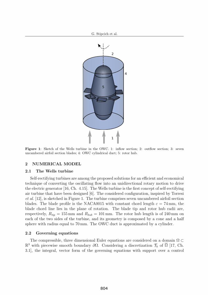
Figure 1: Sketch of the Wells turbine in the OWC. 1: inflow section; 2: outflow section; 3: sevenuncambered airfoil section blades; 4: OWC cylindrical duct; 5: rotor hub.

2 NUMERICAL MODEL

2.1 The Wells turbine

Self-rectifying turbines are among the proposed solutions for an efficient and economicaltechnique of converting the oscillating flow into an unidirectional rotary motion to drivethe electric generator [16, Ch. 4.15]. The Wells turbine is the first concept of self-rectifyingair turbine that have been designed [6]. The considered configuration, inspired by Torresiet al. [12], is sketched in Figure 1. The turbine comprises seven uncambered airfoil sectionblades. The blade profile is the NACA0015 with constant chord length c = 74mm, theblade chord line lies in the plane of rotation. The blade tip and rotor hub radii are,respectively, Rtip = 155mm and Rhub = 101mm. The rotor hub length is of 240mm oneach of the two sides of the turbine, and its geometry is composed by a cone and a halfsphere with radius equal to 70mm. The OWC duct is approximated by a cylinder.

2.2 Governing equations

The compressible, three dimensional Euler equations are considered on a domain Ω ⊂R3 with piecewise smooth boundary ∂Ω. Considering a discretization Th of Ω [17, Ch.3.1], the integral, vector form of the governing equations with support over a control

3

804

G. Stipcich et al.

volume V ⊂ Ω can be cast as [18, Ch. 2]

∂

∂t

∫

V

Q dV =

∫

∂V

F (Q) · n dS (1)

where t denotes time, and the unit vector normal to ∂V is denoted as n. The vector ofconservative variables Q and the non-linear mapping F (Q) are defined, respectively, as

Q =

ρρuρE

F (Q) =

ρuρu⊗ u+ P I

ρHu

(2)

where ρ and P denote, respectively, the density and static pressure, and the velocity vectoris denoted by u. The total energy and enthalpy per unit mass are denoted, respectively,by E and H = E+P/ρ. The symbol ⊗ stays for the tensor product, and I is the identitytensor. System (1-2) is closed by the equation of state for an ideal gas [19, Ch. 2].

2.3 Virtual multiple reference frame

In order to account for the rotary motion of the Wells turbine, the Virtual, MultipleReference Frame technique (VMRF hereafter) is used (see Remaki et al. [13] for details).The VMRF method consists in an alternative algorithm of the Multiple Reference Framemodel (MRF) [15]. The governing equations are transformed into a reference frame thatmoves with steady rotational and/or translational velocity. As a consequence, the un-steady flow in an inertial frame of reference, is approximated as a steady flow in themoving frame of reference. Different speeds can be assigned to different zones of thedomain, and the flow in each zone is solved using the respective moving reference frameequations. The main advantage of the VMRF with respect the original MRF model isthat the former does not require the creation of different meshes for the different zones.

As an example, the zone Ωr ⊂ Ω is assumed to rotate with steady angular velocityω and center of rotation x0. After a coordinate transformation into a frame of referenceattached to Ωr, system (1) results into the VMRF formulation:

∂

∂t

∫

V

Q dV =

∫

∂V

Fr (Q) · n dS +

∫

V

Sr dV (3)

where the non-linear mapping Fr (Q) and the source term Sr read as, respectively

Fr (Q) =

ρ (u− ur)ρu⊗ (u− ur) + P IρH (u− ur) + Pur

Sr =

0−ρ (ω × u)

0

(4)

The symbol ur denotes the velocity due to rotation ur = ω× r, with r being the positionvector pointing from the center of rotation to a generic point x in the domain, i.e. r =x− x0.

The main advantages of the VMRF method can be summarized as follows:

4

805

G. Stipcich et al.

• It is not required to construct different meshes for the different zones. A single meshcan be used for the whole computational domain Ω, as the definition of the rotatingregions Ωr takes place at solver level.

• A steady-state approximation of an unsteady problem is solved, thus saving com-putational cost. This approach can provide reasonable approximations of the time-averaged flow field in turbomachinery applications, where, due to the high valuesof the rotation velocity ω, a poor interaction between the moving and stationaryzones occurs [15].

• A single set of equations (3-4) is used. In fact, although system (3-4) is obtainedthrough a coordinate transformation, it provides the solution for the absolute valuesof the unknown conservative variables Q. It can be noted that, in areas not belong-ing to a rotating region V /∈ Ωr, the angular velocity is zero ω = 0, thus recoveringthe formulation (1-2) for the stationary frame of reference.

3 NUMERICAL SIMULATIONS

The BBIPED Computational Fluid Dynamics (CFD) platform [14] is used for thenumerical simulation of the flow through the OWC described in Section 2.1. The platformrelies on the open source packages SALOME [20], for geometry and grid generation, andon SU2 [21], for the flow solution. The BBIPED CFD platform accommodates ad-hocimplementations that are not present in the original version of the flow solver, such as theVMRF method described in Section 2.3. The aim of the present numerical experiments isto verify the applicability of BBIPED, featuring the VMRF method and a compressiblesolver, to be used for the solution of the relatively low speed flow in the Wells turbine(Mach number ∼ 10−2). Although the overall performance of a turbomachine may dependon phenomena associated with unsteady flow [22], this preliminary analysis accounts forthe steady state only. By solving the inviscid Euler equations, the friction effects on theflow field are neglected.

3.1 Case set-up

Numerical scheme. The SU2 flow solver uses the vertex-based finite volume schemefor the space discretization [18]. The advection term is treated by a second-order accurateRoe-Turkel scheme [23], featuring a second order Venkatakrishnan limiter [24], while thesource term is integrated by a first order piecewise constant method [18]. For the timemarching, a second order accurate implicit Euler scheme is used. The biconjugate gradientstabilized (BCGSTAB) method [25, Ch. 9] is employed for the solution of the resultingimplicit linear system of equations, and, since relatively low Mach numbers are considered,a Turkel preconditioner is employed for facilitating the convergence [26].

Computational domain. The computational domain is sketched in Figure 2. TheOWC’s cylindrical duct is 1400mm long and its radius is equal to Rduct = 165mm. The

5

806

G. Stipcich et al.

1

2

3a3b

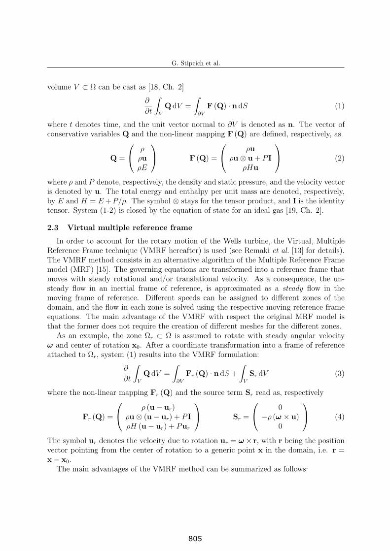
Figure 2: Sketch of the computational domain. 1: inflow section; 2: buffer region; 3a-3b: limits of therotating region for the VMRF.

rotating region Ωr is a cylinder whose axis coincides with the axis of rotation of theturbine, its two bases are located at a distance of 260 and 740mm from the inflow section(labels 3a and 3b in Figure 2).

Boundary and initial conditions. At the inflow section, the imposed boundarycondition is atmospheric pressure and a fixed velocity, parallel to the axis of rotation,according to the value of the considered volumetric flow rate q (see Section 3.2). In orderto model a farfield boundary condition, the outflow section of the cylindrical duct opensin a wider buffer region, the cube E3

buff , where Rduct Ebuff = 1000mm. At the bufferfaces, the imposed boundary condition is atmospheric pressure. At the duct surface andat the turbine’s blades and rotor, a slip boundary condition is imposed. In the wholedomain is imposed an initial condition of uniform velocity field, parallel to the axis ofrotation, according the considered volumetric flow rate q (Section 3.2).

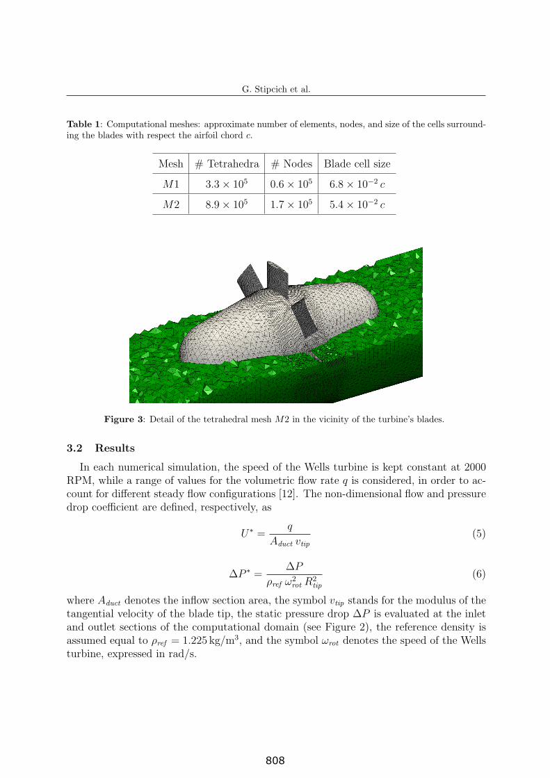
Computational meshes and convergence criteria. The whole domain is dis-cretized by tetrahedral elements. A set of two different meshes M1 and M2 is used, withcoarse and finer cell size, respectively, as specified in Table 1. In both meshes, the regionincluded in a distance of 50mm from the plane of rotation has an element size five timessmaller than the rest of the cylindrical duct. The buffer region is discretized by using avery coarse element size, roughly fifty times larger than in the cylindrical duct. Figure 3shows a detail of the mesh M2 in the vicinity of the blades.

The steady state of the flow solution is reached and the simulation is considered con-verged afterwards the residuals of the conserved variables Q have dropped of at least 3orders of magnitude.

6

807

G. Stipcich et al.

Table 1: Computational meshes: approximate number of elements, nodes, and size of the cells surround-ing the blades with respect the airfoil chord c.

Mesh # Tetrahedra # Nodes Blade cell size

M1 3.3× 105 0.6× 105 6.8× 10−2 c

M2 8.9× 105 1.7× 105 5.4× 10−2 c

Figure 3: Detail of the tetrahedral mesh M2 in the vicinity of the turbine’s blades.

3.2 Results

In each numerical simulation, the speed of the Wells turbine is kept constant at 2000RPM, while a range of values for the volumetric flow rate q is considered, in order to ac-count for different steady flow configurations [12]. The non-dimensional flow and pressuredrop coefficient are defined, respectively, as

U∗ =q

Aduct vtip(5)

∆P ∗ =∆P

ρref ω2rot R

2tip

(6)

where Aduct denotes the inflow section area, the symbol vtip stands for the modulus of thetangential velocity of the blade tip, the static pressure drop ∆P is evaluated at the inletand outlet sections of the computational domain (see Figure 2), the reference density isassumed equal to ρref = 1.225 kg/m3, and the symbol ωrot denotes the speed of the Wellsturbine, expressed in rad/s.

7

808

G. Stipcich et al.

0.1 0.14 0.18 0.22 0.260.2

0.4

0.6

0.8

U∗

∆P

∗

Coarse mesh M1Fine mesh M2

Experimental

RSM

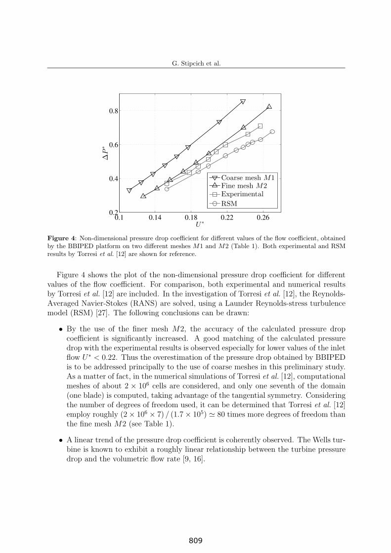
Figure 4: Non-dimensional pressure drop coefficient for different values of the flow coefficient, obtainedby the BBIPED platform on two different meshes M1 and M2 (Table 1). Both experimental and RSMresults by Torresi et al. [12] are shown for reference.

Figure 4 shows the plot of the non-dimensional pressure drop coefficient for differentvalues of the flow coefficient. For comparison, both experimental and numerical resultsby Torresi et al. [12] are included. In the investigation of Torresi et al. [12], the Reynolds-Averaged Navier-Stokes (RANS) are solved, using a Launder Reynolds-stress turbulencemodel (RSM) [27]. The following conclusions can be drawn:

• By the use of the finer mesh M2, the accuracy of the calculated pressure dropcoefficient is significantly increased. A good matching of the calculated pressuredrop with the experimental results is observed especially for lower values of the inletflow U∗ < 0.22. Thus the overestimation of the pressure drop obtained by BBIPEDis to be addressed principally to the use of coarse meshes in this preliminary study.As a matter of fact, in the numerical simulations of Torresi et al. [12], computationalmeshes of about 2 × 106 cells are considered, and only one seventh of the domain(one blade) is computed, taking advantage of the tangential symmetry. Consideringthe number of degrees of freedom used, it can be determined that Torresi et al. [12]employ roughly (2× 106 × 7) / (1.7× 105) 80 times more degrees of freedom thanthe fine mesh M2 (see Table 1).

• A linear trend of the pressure drop coefficient is coherently observed. The Wells tur-bine is known to exhibit a roughly linear relationship between the turbine pressuredrop and the volumetric flow rate [9, 16].

8

809

G. Stipcich et al.

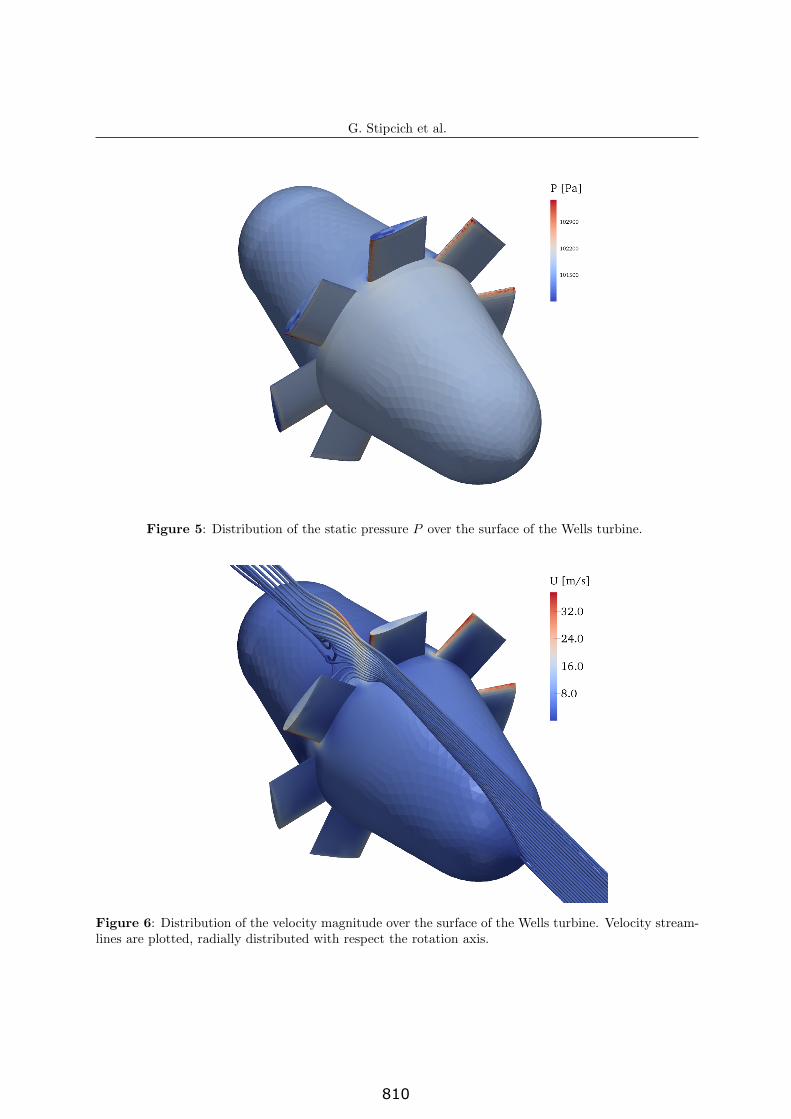
Figure 5: Distribution of the static pressure P over the surface of the Wells turbine.

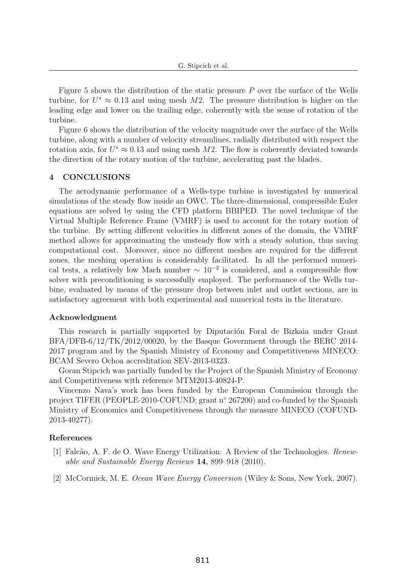
Figure 6: Distribution of the velocity magnitude over the surface of the Wells turbine. Velocity stream-lines are plotted, radially distributed with respect the rotation axis.

9

810

G. Stipcich et al.

Figure 5 shows the distribution of the static pressure P over the surface of the Wellsturbine, for U∗ ≈ 0.13 and using mesh M2. The pressure distribution is higher on theleading edge and lower on the trailing edge, coherently with the sense of rotation of theturbine.

Figure 6 shows the distribution of the velocity magnitude over the surface of the Wellsturbine, along with a number of velocity streamlines, radially distributed with respect therotation axis, for U∗ ≈ 0.13 and using mesh M2. The flow is coherently deviated towardsthe direction of the rotary motion of the turbine, accelerating past the blades.

4 CONCLUSIONS

The aerodynamic performance of a Wells-type turbine is investigated by numericalsimulations of the steady flow inside an OWC. The three-dimensional, compressible Eulerequations are solved by using the CFD platform BBIPED. The novel technique of theVirtual Multiple Reference Frame (VMRF) is used to account for the rotary motion ofthe turbine. By setting different velocities in different zones of the domain, the VMRFmethod allows for approximating the unsteady flow with a steady solution, thus savingcomputational cost. Moreover, since no different meshes are required for the differentzones, the meshing operation is considerably facilitated. In all the performed numeri-cal tests, a relatively low Mach number ∼ 10−2 is considered, and a compressible flowsolver with preconditioning is successfully employed. The performance of the Wells tur-bine, evaluated by means of the pressure drop between inlet and outlet sections, are insatisfactory agreement with both experimental and numerical tests in the literature.

Acknowledgment

This research is partially supported by Diputacion Foral de Bizkaia under GrantBFA/DFB-6/12/TK/2012/00020, by the Basque Government through the BERC 2014-2017 program and by the Spanish Ministry of Economy and Competitiveness MINECO:BCAM Severo Ochoa accreditation SEV-2013-0323.

Goran Stipcich was partially funded by the Project of the Spanish Ministry of Economyand Competitiveness with reference MTM2013-40824-P.

Vincenzo Nava’s work has been funded by the European Commission through theproject TIFER (PEOPLE-2010-COFUND; grant n 267200) and co-funded by the SpanishMinistry of Economics and Competitiveness through the measure MINECO (COFUND-2013-40277).

References

[1] Falcao, A. F. de O. Wave Energy Utilization: A Review of the Technologies. Renew-able and Sustainable Energy Reviews 14, 899–918 (2010).

[2] McCormick, M. E. Ocean Wave Energy Conversion (Wiley & Sons, New York, 2007).

10

811

G. Stipcich et al.

[3] Heath, T., Whittaker, T. J. T. & Boake, C. B. The Design, Construction andOperation of the LIMPET Wave Energy Converter (Islay, Scotland). In Proceedingsof 4th European Wave Energy Conference, 49–55 (2001).

[4] Falcao, A. F. de O. The Shoreline OWC Wave Power Plant at the Azores. InProceedings of 4th European Wave Energy Conference, 42–48 (2001).

[5] Torre-Enciso, Y., Ortubia, I., Lopez de Aguileta, L. I. & Marque, J. Mutriku WavePower Plant: from the thinking out to the reality. In Proceedings of 8th EuropeanWave and Tidal Energy Conference, 319–329 (2009).

[6] Wells, A. A. Fluid Driven Rotary Transducer. British Patent 1595700 (1976).

[7] Raghunathan, S. A Methodology for Wells Turbine Design for Wave Energy Con-version. Proceedings of the Institution of Mechanical Engineers, Part A: Journal ofPower and Energy 31, 221–232 (1995).

[8] Mohamed, M. H., Janiga, G., Pap, E. & Thevenin, D. Multi-Objective Optimizationof the Airfoil Shape of Wells Turbine Used for Wave Energy Conversion. Energy 36,438–446 (2011).

[9] Brito-Melo, A., Gato, L. M. C. & Sarmento, A. J. N. A. Analysis of Wells Tur-bine Design Parameters by Numerical Simulation of the OWC Performance. OceanEngineering 29, 1463–1477 (2002).

[10] Setoguchi, T., Santhakumar, S., Takao, M., Kim, T. H. & Kaneko, K. A ModifiedWells Turbine for Wave Energy Conversion. Renewable Energy 28, 79–91 (2003).

[11] Setoguchi, T. & Takao, M. Current Status of Self Rectifying Air Turbines for WaveEnergy Conversion. Energy Conversion and Management 47, 2382–2396 (2006).

[12] Torresi, M., Camporeale, S. M. & Pascazio, G. Detailed CFD Analysis of the SteadyFlow in a Wells Turbine Under Incipient and Deep Stall Conditions. Journal of FluidsEngineering 131 (2009).

[13] Remaki, L., Ramezani, A., Blanco, J. M. & Antolin, J. I. Efficient Rotating FrameSimulation in Turbomachinery. In Proceedings of ASME Turbo Expo 2014: TurbineTechnical Conference and Exposition, vol. 2B (2014).

[14] BCAM - Basque Center for Applied Mathemathics. BBIPED, CFD Industrial Plat-form for Engineering Design (2015). URL http://www.bcamath.org/es/research/

lines/CFDMS/software.

[15] Luo, J. Y., Issa, R. I. & Gosman, A. D. Prediction of Impeller-Induced Flows inMixing Vessels Using Multiple Frames of Reference. In I ChemE Symposium Series,vol. 136, 549–556 (1994).

11

812

G. Stipcich et al.

[16] Dixon, S. L. Fluid Mechanics and Thermodynamics of Turbomachinery (ElsevierButterworth-Heinemann, Boston, 2013), 5th edn.

[17] Quarteroni, A. & Valli, A. Numerical Approximation of Partial Differential Equations(Springer-Verlag Italia, Milano, 1994).

[18] Blazek, J. Computational Fluid Dynamics: Principles and Applications (Elsevier,Amsterdam, 2001), 2nd edn.

[19] Anderson, J. D. Computational Fluid Dynamics (Mc Graw Hill, New York, 1995),3rd edn.

[20] OPEN CASCADE. SALOME, The Open Source Integration Platform for NumericalSimulation (2015). URL http://www.salome-platform.org/.

[21] Stanford University Aerospace Lab. SU2, The Open-Source CFD Code (2015). URLhttp://su2.stanford.edu/index.html.

[22] Greitzer, E. M. Introduction to Unsteady Flow in Turbomachines. In Von KarmanInst. for Fluid Dynamics Unsteady Flow in Turbomachines, vol. 1 (1984).

[23] Viozat, C. Implicit Upwind Schemes for Low Mach Number Compressible Flows.Tech. rep., Institut National de Recherche en Informatique et en Automatique (1997).

[24] Venkatakrishnan, V. On The Accuracy of Limiters and Convergence to Steady StateSolutions. Tech. Rep. AIAA-93-088, American Institute of Aeronautics and Astro-nautics (1993).

[25] van der Vorst, H. A. Iterative Krylov Methods for Large Linear Systems (ElsevierButterworth-Heinemann, New York, 2003).

[26] Turkel, E. Preconditioning Techniques in Computational Fluid Dynamics. In AnnualReview of Fluid Mechanics, vol. 31, 385–416 (1999).

[27] Launder, B. E. Second-Moment Closure and its Use in Modelling Turbulent IndustrialFlows. International Journal for Numerical Methods in Fluids 9, 963–985 (1989).

12

813