A numerical investigation into the correction algorithms for SPHmethod in modeling violent free surface flows

M. Ozbulut a, M. Yildiz b,n, O. Goren a

a Faculty of Naval Architecture and Ocean Engineering, Istanbul Technical University, Istanbul, Turkeyb Faculty of Engineering and Natural Sciences, Sabanci University, Istanbul, Turkey

a r t i c l e i n f o

Article history:Received 7 January 2013Received in revised form10 November 2013Accepted 27 November 2013Available online 11 December 2013

Keywords:Violent free surface flowsSPHCorrection algorithms

a b s t r a c t

A quantitative comparison of the usual and recent numerical treatments which are applied to theSmoothed Particle Hydrodynamics (SPH) method are presented together with a new free-surfacetreatment. A series of numerical treatments are studied to refine the numerical procedures of the SPHmethod particularly for violent flows with a free surface. Two dimensional dam-break and sway-sloshingproblems in a tank are modeled by solving Euler's equation of motion utilizing weakly compressible SPHmethod (WCSPH). Initially, the dam-break benchmark problem is studied by adopting only conventionalbasic equations of SPH without any numerical remedy and then by considering numerical treatments ofinterest one after another. In the WCSPH method, the precise calculation of the densities of the particlesis vital for the solution, accordingly a density correction algorithm is presented as a basic numericaltreatment. Subsequently, Monaghan's (1994) [1] XSPH velocity variant algorithm, artificial particledisplacement (APD) algorithm (Shaldoo et al., 2011) [2], and a hybrid combination of velocity updatedXSPH (VXSPH) and APD algorithms are implemented separately, but all with the density correctionalgorithm as a default treatment. The effects of each of these treatments on the pressure and on the freesurface profiles are analyzed by comparing our numerical findings with experimental and numericalresults in the literature. After the detailed scrutiny on the dam-break problem, sway-sloshing problem ishandled with the VXSPHþAPD algorithm which has been noted to provide the most reliable andaccurate results in the dam-break problem. For the sway-sloshing problem, the time histories of freesurface elevations on the left side wall of the rectangular tank are compared with experimental andnumerical results available in the literature. It was shown that the VXSPHþAPD treatment significantlyimproves the accuracy of the numerical simulations for violent flows with a free surface and lead to theresults which are in very good agreement with experimental and numerical findings of literature interms of both the kinematic and the dynamic point of view.

1. Introduction

Due to its Lagrangian and meshless nature, the Smoothed ParticleHydrodynamics (SPH) method is an exceptionally suitable tool formodeling highly nonlinear violent flows with a free surface. The SPHmethod was introduced simultaneously by Gingold and Monaghan[3] and Lucy [4] to simulate compressible flow problems in astro-physics and later extended by Monaghan [1] to model incompres-sible free surface flows through using a Weakly Compressible SPHapproach (WCSPH) which assumes that a fluid is incompressible if itsdensity variation is less than 1%. In the SPH method, the continuumis represented by particles which carry fluid properties such as

density, velocity and pressure, among others. These particles repre-sent infinitesimally small fluid elements having finite volumes, andcan interact with each other in each time-step through a weightfunction having a compact support domain. The relevant governingequations and boundary conditions are discretized in space overthese particles. Although the WCSPH method has numerous advan-tages on solving nonlinear engineering problems with large andrapid deformations in the topology of fluid such as shock [5], highvelocity impact [6], underwater explosion [7] and violent free surfacehydrodynamics [8] problems, it still requires a detail scrutiny tounderstand the effect of numerical remedies (i.e., particle distributionregularization through XSPH, density correction, and some others)incorporated into the standard WCSPH method on the accuracy ofthe solution. As shown in our earlier work [9] as well as in anotherwork by Molteni and Colagrossi [10], the kinematics of violent flowswith free surface might be easily captured correctly to a certainextent by using the conventional WCSPH algorithm with commonly

http://dx.doi.org/10.1016/j.ijmecsci.2013.11.021

n Corresponding author.E-mail addresses: ozbulutm@itu.edu.tr (M. Ozbulut),

meyildiz@sabanciuniv.edu (M. Yildiz).

used formulations in the SPH literature. However, noting that theWCSPH method is known to produce an oscillatory pressure fielddue to the fact that the pressure is calculated from density variationthrough an equation of state [10,11], the existence of large andrandom oscillations in the pressure field urges SPH practitionersto develop new numerical correction algorithms to have realisticpressure values.

In order to circumvent pressure related problems, there havebeen some attempts whereby to improve the accuracy, stabilityand robustness of numerical solution. In addition to Monaghan's[12] “artificial viscosity” and “XSPH velocity variant” terms whichhave received noticeable acceptance, and in turn have been widelyused by SPH researchers, new numerical remedies or correctivealgorithms have also been incorporated into SPH method in recentstudies. Molteni and Colagrossi [10] added a density diffusion terminto the mass conservation equation, which is a pure numericaleffect and goes to zero as the number of particles increases.To prevent particle penetration, Zheng and Duan [13] added anextra position corrector term to the positions of the particles.They stated that this additional term has a positive effect on thehomogeneous distribution of particles which leads better pressurefields in the problem domain.

Present work compares numerical remedies namely, densitycorrection, XSPH velocity variant algorithm commonly used in theSPH literature among each other and with a relatively recent onereferred to as Artificial Particle Displacement (APD) [2]. It alsointroduces a new treatment for free surface problems, which uses ahybrid combination of velocity updated XSPH, which is hereafterreferred to as VXSPH, algorithm for the free surface particles andAPD for the rest of fluid particles. Two dimensional dam-breakproblem, which is quite well-accepted as a benchmark test caseamong SPH researchers, is solved using Euler's equation of motion.Having validated the numerical results by those given in theliterature for the dam-break problem, a two dimensional sway-sloshing problem is modeled to further test the numerical treat-ment which has been observed to give the most accurate andreliable results in the numerical stimulation of dam-break problem.

The present work initially considers the numerical modeling ofthe dam-break problem through employing the conventional basicformulations of the WCSPH method together with the artificialviscosity term. It is understood that the standard WCSPH formula-tions without any numerical remedies lead to significant oscilla-tions in density field and in turn in pressure distributions, therebyresulting in particle deficient region (a gap) in the vicinity of thesolid wall at the front edge of the flow. In order to eliminate thenoise in pressure field, the density correction treatment isemployed as a numerical remedy to the conventional WCSPHmethod since the pressure value of a particle is calculated by anartificial equation of state [14], which directly relates the densityand pressure of particles. The density correction is considered as abaseline treatment while other three numerical treatments(namely, XSPH, APD, and VXSPH) modeled here are used togetherwith the density correction algorithm individually or in a com-bined manner. The density correction treatment is applied in thepredictor step and the new pressures are computed by using thecorrected density values.

After confining the pressure oscillations within an admissiblerange by using the density correction algorithm, the effects of theother three different numerical remedies on the pressure, on the freesurface elevation and on the total mechanical energy of the fluidparticles are investigated systematically. The first of these treatmentsis the well-known XSPH algorithm which was suggested by Mon-aghan [1] for high speed free surface flows to keep the particlesorderly and to prevent a particle penetration one by another.The second one is the method implemented in order to eliminateparticle clustering and fractures due to the tendency of SPH particles

to follow streamline trajectories, wherefore a more homogeneousparticle distribution can be achieved in the computational domain.Presently, the APD method is further extended to a flow problemwith a violent free surface since in the literature it was originallyused for flow problems with bounding solid boundaries [15]. In thelight of the results of the first two remedies, the hybrid combinationof APD and VXSPH algorithms is used wherein the VXSPH methodis applied only to the particles near the free surface and theAPD treatment is applied only to fluid regions away from the freesurface and fully populated with particles. In SPH modeling of freesurface problems, particles may escape from free surface, which is anumerical artifact and becomes muchmore noticeable as the velocityand the non-linearity of the flow increases. The VXSPH algorithmprovides an artificial surface tension force for free surface particlesthereby impeding the escape of individual particles from the freesurface and keeping these particles being attached to the free surface.The results of simulations for the dam-break problem show that thecombined usage of VXSPH and APD treatments gives the mostreliable and admissible results from both kinematical and dynamicalpoint of view. The VXSPH-APD hybrid treatment used in the dam-break problem is further validated for another challenging freesurface problem, namely, two dimensional sway-sloshing whereinthe free surface elevations on the left side wall are compared withthe experimental data and numerical solutions of the studies givenby Pakozdi [16] and Molteni [10].

2. Governing equations and numerical modeling

2.1. Field equations

In the free surface hydrodynamics, the effect of viscosity isgenerally assumed to be negligible and the fluid particles areallowed to have rotational motion which leads the equation ofmotion governed by Euler's equation:

du!dt

¼ �1ρ∇Pþ g! ð1Þ

u!¼ d r!dt

ð2Þ

where, u!; r!, P and ρ are the velocity, position, pressure and

density of particles, respectively, and g! is the gravitationalacceleration. In addition to Euler's equation of motion, the con-tinuity equation employed is as follows:

dρdt

¼ �ρ∇ � u!: ð3Þ

In the SPH method, there are two general approaches for enforcingthe incompressibility condition, namely, the weakly compressibleSPH (WCSPH), and the incompressible SPH (ISPH) methods, whichdiffer from each other in terms of how the pressure in theequation of motion is computed. The WCSPH method uses anexplicit artificial equation of state that couples the density withthe pressure through a coefficient widely referred to as the speedof sound. This approach stems from the initial applications of theSPH method to the compressible fluid flow problems on the factthat all fluids may be regarded as weakly compressible, at leasttheoretically. The equation of state enforce the incompressibilitycondition on the flow such that a small variation in densityproduces a relatively large change in pressure thereby limitingthe dilatation of the fluid to one percent. The ISPH technique isbased on the projection method originally proposed in [17], whichis referred to as the standard projection or the divergence-freeISPH method. In this method, the pressure term in the equation ofmotion is computed by solving a pressure Poisson equation with

the divergence of the intermediate velocity being a source term.There are several recent works which have aimed to compareWCSPH and ISPH methods for free surface and bluff body pro-blems [17,18]. Major advantages of WCSPH over ISPH are the easeof programming, and better ordered particle distributions. Mainlyfor these reasons, the WCSPH method has become the mostwidespread approach to solve the linear momentum balanceequation in the SPH literature. The standard WCSPH approachrequires the usage of a Mach (M) number (a dimensionlessquantity representing the ratio of speed of fluid to speed of sound)less than 0.1 to ensure that the flow is incompressible and to avoidthe formation of unphysical void regions in the computationaldomain. The WCSPH approach unlike the ISPH method needs touse extremely small time steps in order to satisfy the Courant–Friedrichs–Lewy (CFL) condition since the speed of sound has adirect effect on the permissible time-step in a given simulation,which directly affects the total simulation time [2,19]. There arevarious forms of artificial equation of state used within the scopeof WCSPH approach to be able to calculate the pressure forcomputing pressure gradient term in the equation of motion. Inthis work, the one proposed by Monaghan [12] is used:

p¼ ρ0c20

γρρ0

� �γ

�1� �

; ð4Þ

where c0 is the reference speed of sound, γ is the specific heat-ratioof water and is equal to 7 and ρ0 is the reference density which isequal to 1000 [kg/m3] for fresh water. The value of reference speedof sound is determined by M. It is required that M � 0:1 to keepdensity variation around 1% [12]. The key point in Eq. (4) is that avery small variation in the density of the fluid particle leads to arelatively large change in pressure whereby the volume change ofparticles is restricted around 1%. Furthermore, it should be notedthat the larger the value of c0, the smaller the value of permissibletime step, Δt due to the CFL stability condition. Hence, to avoid theunnecessary increase in the computational time, c0 should be smallenough while guaranteeing the incompressibility condition. In thesimulations of the dam-break and sway-sloshing problems, c0 istaken as 50 [m/s] and 40 [m/s], respectively.

2.2. Discretization of governing equations in SPH method

SPH is a Lagrangian method where the flow domain is repre-sented by a finite number of movable particles which can carry thecharacteristic properties of the problem at hand such as mass,position, velocity, momentum, and energy. The core of its math-ematical formulation is based on the interpolation process, where-fore the fluid system is modeled through the interaction amongparticles, which is achieved by an analytical function widelyreferred to as the kernel/weighting function Wðrij;hÞ where rij isthe magnitude of the distance vector, r!ij ¼ r!i� r!j for a pair ofparticles, namely, the particle of interest i and its neighboringparticles j, and h is the smoothing length. Here, r!i and r!j are theposition vectors for the particle i and j, respectively, and as to beunderstood, boldface indices i and j are particle identifiers todenote particles. An arbitrary continuous function (which can bescalar, vectorial, or tensorial), Að r!iÞ, or concisely denoted as Ai, canbe interpolated as

Aiffi ⟨Að r!iÞ⟩�ZΩAð r!jÞWðrij;hÞd3 r!ij; ð5Þ

where the angle bracket “⟨⟩” denotes the kernel approximation,d3 r!ij is the infinitesimal volume element inside the domain,and Ω represents the total bounded volume of the domain.The function Ai may represent any hydrodynamic properties suchas velocity, pressure, density, and viscosity. The kernel function

used in the current work is a quintic spline with the form of

WðR;hÞ ¼ αd

ð3�RÞ5�6ð2�RÞ5þ15ð1�RÞ5; 0rRo1ð3�RÞ5�6ð2�RÞ5; 1rRo2ð3�RÞ5; 2rRo30; RZ3

8>>>><>>>>:

9>>>>=>>>>; ð6Þ

where R¼ rij=h and αd is a coefficient that depends on thedimension of the problem such that 120/h, 7=ð478πh2Þ and3=ð359πh3Þ for one, two and three dimensions, respectively [20].Upon using the SPH approximations which involve the replace-ment of the integral operation over the volume of the boundeddomain by the mathematical summation operation over all neigh-boring particles j of the particle of interest i, and the differentialvolume element by the mj=ρj, and performing some tediousmathematical manipulations, the Euler's equation of motion andthe mass conservation can respectively be discretized by the SPHmethod as

du!i

dt¼ � ∑

N

j ¼ 1

piρ2i

þ pjρ2j

þΠij

!∇iW ij ð7Þ

dρi

dt¼ ρi ∑

N

j ¼ 1

mj

ρjðu!i� u!jÞ � ∇iW ij: ð8Þ

Here, mj is the mass of the particle j, ∇i is the gradient operatorwhere the particle identifier i indicates the spatial derivative isevaluated at particle position i, and Πij is the artificial viscosityterm as

Πij ¼�αμij

ci þ cjρi þρj

; u!ij � r!ijo0

0; u!ij � r!ijZ0

8<:9=;; ð9Þ

μij ¼ hðu!i� u!jÞ � ð r!i� r!jÞ‖ r!i� r!j‖2þθh2

: ð10Þ

The inclusion of the artificial viscosity term in the Euler equation ofmotion is necessary to increase the stability of the numericalprocedures through adding some diffusion to numerical solution.However, the magnitude of the artificial viscosity coefficient shouldalso be small enough to prevent the occurrence of the viscous effectsduring the fluid flow. The numerical value of α utilized in this work isdetermined through comparing the obtained numerical results withbenchmark solutions. In the simulation of dam-break and sway-sloshing problems, the parameters α and θ are taken as 0.06 and0.05, respectively. The local speed of sounds in Eq. (9) is foundaccording to the relation ci ¼ coðρi=ρoÞðγ�1Þ=2.

2.3. Boundary conditions

The accurate force transfer from solid boundary particles ontothe fluid particles is modeled through utilizing ghost particletechnique whereby fluid particles, having a vertical distance lessthan 1.55 h from the solid boundary, or in other words, within thesupport domain of boundary particles, are mirrored with respectto the solid wall to create ghost particles outside the flow domain.Ghost particles are endowed with field variables (i.e., velocity andpressure) in accordance with the boundary conditions to beimplemented. For the Dirichlet boundary condition, the followinglinear interpolation is employed; namely, Λg ¼ 2Λb�Λf while forthe Neumann boundary condition, ghost particles are given thesame fields values as their corresponding fluid particles, andhence, Λg ¼Λf , where Λg, Λb, and Λf are in the given orderrepresent the fields variables associated with the ghost, boundary,and fluid particles. In the simulations of present work for bothdam-break and sway-sloshing problems, walls are modeled with

free slip boundary condition. In dam-break problem, for thehorizontal wall, the ghost particle velocities are evaluated by∂ux=∂z¼ 0, and uz¼0, necessitating that ux;g ¼ ux;f anduz;g ¼ �uz;f while for the vertical walls, ∂uz=∂x¼ 0, and ux¼0,requiring that uz;g ¼ uz;f and ux;g ¼ �ux;f [2]. As for the boundaryconditions for the sway-sloshing problem where the walls have aharmonic motion, the free slip boundary condition on the hor-izontal wall requires ux;g ¼ 2ux;b�ux;f and uz;g ¼ �uz;f , and forthe vertical walls it requires that ux;g ¼ 2ux;b�ux;f and uz;g ¼ uz;f .The pressure boundary condition on the solid walls is enforced as∇p � n!¼ 0, which requires that ρg ¼ ρf and pg¼pf. As in the case offluid particles, the density of boundary particles is computedthrough the solution of the continuity equation given in Eq. (3)and these densities are smoothed by using Eq. (12). Upon deter-mining the density of boundary particles calculated, pressure ofboundary particles is computed by the usage of previouslyintroduced equation of state. Due to the dynamic nature of theproblems solved in this work, some boundary particles may nothave enough neighboring fluid particles for accurate calculation ofdensity of boundary particles. In such a case, these boundaryparticles should not feel any pressure force from surrounding fluidparticles. Owing to the density correction through smoothing,boundary particles with no or insufficient neighboring fluidparticles will acquire density and in turn pressure because of thetransfer of data among boundary particles. To avoid this, and beable to calculate the pressure of boundary particles correctly, thedensity of boundary particles with less than ten fluid particles isset back to reference density, which corresponds to enforcing zeropressure for these boundary particles. The free surface boundarycondition is enforced by setting the pressure of particles close tofree surface to the atmospheric pressure through taking thedensities of these particles as reference density. The decisionwhether a particle should be regarded as a free surface particledepends on the number of neighbor particles of the given particle.In the simulations presented, the average number of neighborparticles is around 40–45 at each time step. Thus, a fluid particlewith less than twenty-five neighbors is considered as a freesurface particle.

2.4. Time integration

The time integration scheme used in this work is a predictor–corrector one wherein particle positions, densities and velocitiesare updated in the following manner, respectively:

d r!i

dt¼ u!i;

dρi

dt¼ ki;

du!i

dt¼ a!i: ð11Þ

The time integration starts with the prediction of the intermediate

positions and densities of the particles by r!ðnþ1=2Þi ¼

r!ðnÞi þ0:5u!n

iΔt and ρðnþ1=2Þi ¼ ρn

i þ0:5kðnÞi Δt. The pressure valuesare calculated from Eq. (4) by using the intermediate densities

while new time steps' velocities are computed by u!ðnþ1Þi ¼

u!ðnÞi þ a!ðnþ1=2Þ

i Δt. Finally, at the corrector step, the particle positions

and densities are updated at half time step as r!ðnþ1Þi ¼

r!ðnþ1=2Þi þ0:5u!ðnþ1Þ

i Δt and ρðnþ1Þi ¼ ρðnþ1=2Þ

i þ0:5kðnþ1Þi Δt.

The superscript n is a temporal index.

3. Numerical treatments

The main focus of this paper is on the comparison of the effectsof different numerical remedies on the accuracy and robustness ofthe WCSPH method. These remedies include density (Shephard)

correction, XSPH velocity correction, and artificial particle displa-cement (APD), which have been widely utilized in the SPHliterature to circumvent the short comings of standard SPHformulations such as pressure oscillation, non-uniform and clus-tered particle distributions, among others. To be able to quantifythe effects of these treatments on the numerical results and alsobe able investigate their hybrid usage, two important benchmarkproblems, namely dam-break and sway-sloshing, are modeled.The dam-break problem is solved using all these remedies andresults are compared to each other in terms of free surface profilesand pressure contours before fluid particles hit to the right wall.Moreover, for each remedy, the pressure values time series at apoint on the right vertical wall are compared with the experi-mental data given in the literature [10,16] after the fluid particleshit to the right wall. For the sake of completeness, in following weconcisely elaborate on each individual numerical remedy whichare listed previously.

Density correction algorithm: In the WCSPH approach, theprecise calculation of density field is very critical since thepressure is directly coupled to density through the artificialequation of state. Without the density correction treatment, thepressure fields in the problem domain can oscillate excessively andbecome unstable due to the numerical noise generated in thestandard SPH formulations. The inclusion of the density correctionalgorithm into the numerical scheme notably improves pressuredistributions, especially close to the solid boundaries. In this work,the density correction is used as a baseline treatment and alwaysemployed with other numerical remedies through the formulation

bρi ¼ ρi�s∑N

j ¼ 1ðρi�ρjÞW ij

∑Nj ¼ 1W ij

ð12Þ

where bρ is the corrected density, N is the number of neighborparticles for particle i and s is a constant which is set to unity inthis work thereby leading to well-known “Shephard” interpolationin the SPH literature [21].

XSPH velocity variant algorithm: It is to be noted that in the SPHmethod, the order of particles affects the accuracy of interpola-tions for the computations of gradient and Laplacian of fields.Therefore, for computational stability and accuracy, it is highlydesirable to move the particles in a more orderly fashion.To achieve this, Monaghan [1] proposed and utilized the XSPHvelocity variant algorithm for free surface flows which later hasbecome one of the widely used and well-known numericalremedies for improving the particle distribution. In the XSPHmethod, the velocity computed through the solution of equationof motion is modified such that it includes the contribution fromneighboring particles, thereby coaxing fluid particles to move with

a velocity (similar to the average velocity), u!xsph

i ¼ u!i�Δu!i

through advection equation d r!i=dt ¼ u!xsph

i where Δu!i is thevelocity variant defined as

Δu!i ¼ ɛ ∑N

j ¼ 1

mj

ρijðu!i� u!jÞW ij: ð13Þ

Here, ρij ¼ ðρiþρjÞ=2 and ɛ is a constant commonly taken as 0.5 inthe SPH literature [16]. To avoid the error due to the densityfluctuations in the velocity variant, it is prudent to modify Eq. (13)as

Δu!i ¼ ɛ∑N

j ¼ 1ðu!

i� u!jÞW ij

∑Nj ¼ 1W ij

ð14Þ

Artificial particle displacement (APD) algorithm: Being a numericaltool based on interpolation theory, the SPH method requires thatparticles be distributed as uniformly as possible for the robustnessand the accuracy of numerical models. If particles in the problem

domain acquire a non-uniform and clustered distribution as a resultof solution, it is no longer possible to retain the stability and thereliability of numerical results, and in extreme cases, the numericalalgorithm may break down. Shadloo et al. [2] in flow simulationswith bounded domains added a small artificial particle displace-ment term to the position vectors of each particle to disturb theparticle trajectory thereby impeding particle clustering and showedthat the APD method is extremely effective in preserving particleuniformity, and in turn improving the both the robustness and theaccuracy of the SPH computation. The APD term δ r!i is given as

δ r!i ¼ β ∑N

j ¼ 1

r!ij

r3ijr2ovmax Δt ð15Þ

where β is a parameter which is equal to 0.05 in this work,ro ¼∑jrij=N is the cut-off distance and vmax is the maximumvelocity in the problem domain in every time step. The parameterβ should be small enough not to change the physics of the flow andlarge enough for providing a homogeneous and uniform particledistribution. In this work, the numerical value of the coefficient β ischosen relying on the simulation results of many different bench-marks problems solved in our previous works [2,15]. Additionally, itis noted that the value of APD added to the numerical simulations isless than 0.1% of the physical particle displacement for a given timestep. Hence, one may directly conclude that the APD does not alterthe neighbors of the given particle of interest, and thus do notintroduce errors to the solution that changes the physics of theproblem at hand. The APD algorithm is employed only for fullypopulated flow regions.

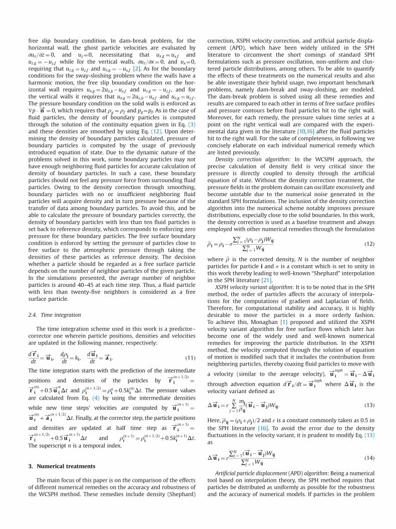
Combined XSPH and APD algorithm: The treatment of free surfaceis always a challenge in the modeling of hydrodynamics andgenerally requires a special care to obtain accurate surface profile.A combined usage of XSPH and APD treatments is also investigatedas a final numerical remedy where a slightly different implementa-tion of standard XSPH algorithm is used only for the particles on thefree surface while the APD algorithm is employed for the fullypopulated flow regions. The physical regions in the computationaldomain where the algorithms are applied are illustrated in Fig. 1.

Recall that in the standard XSPH algorithm, the velocity variantis appended to the velocity when advancing the particle positiononly, but does not affect the velocity used for other SPH calcula-tions. On the other hand, in the hybrid treatment presented here,

the XSPH velocity u!xsph

i is utilized for both advancing the position

of particles and replacing the fluid velocity, namely, u!i ¼ u!xsph

i ,which means that the fluid velocity computed through the solu-tion of the equation of motion is substituted by the averagevelocity. This modified velocity is then used for all other SPHcalculations such as the solution of mass and momentum balanceequations for density and velocity. This new treatment is hereafterreferred to as velocity updated XSPH algorithm with the abbrevia-tion of VXSPH. Since the VXSPH is applied only to a very thin free

surface layer (like first two rows of free surface particles), it doesnot change the physical behavior of the flow. The VXSPH acts like asurface tension force thus keeping particles orderly on the freesurface. The ɛ parameter for VXSPH treatment is chosen to berelatively smaller than the one for XSPH with the numerical valuesof 0.0025 in the dam-break and 0.005 in the sway-sloshingsimulations. The APD treatment on the other hand disturb thetrajectories that particles follow whereby to result in more homo-geneous particle distribution in the fully populated areas.

4. Numerical results

The numerical treatments explained in the previous section areapplied to the two dimensional dam-break problem sequentiallyand the effect of each treatment on the results is presentedcomparatively. Subsequently, the numerical treatment that givesphysically the most reasonable and accurate results in the dam-break problem is used for the two dimensional sway-sloshingproblem and numerically computed free surface elevations on thewalls of the tank are compared with the experimental resultsgiven in [16].

4.1. Dam-break problem: the comparison of the numericaltreatments

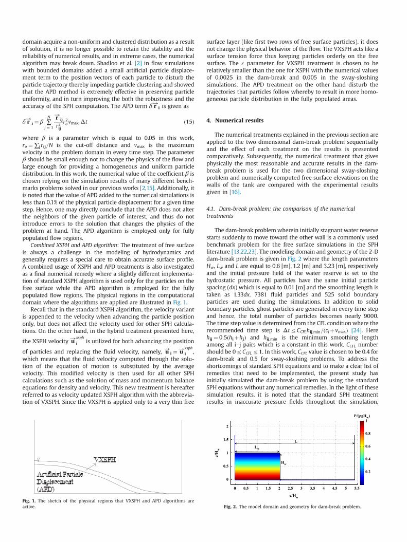
The dam-break problemwherein initially stagnant water reservestarts suddenly to move toward the other wall is a commonly usedbenchmark problem for the free surface simulations in the SPHliterature [13,22,23]. The modeling domain and geometry of the 2-Ddam-break problem is given in Fig. 2 where the length parametersHw, Lw and L are equal to 0.6 [m], 1.2 [m] and 3.23 [m], respectivelyand the initial pressure field of the water reserve is set to thehydrostatic pressure. All particles have the same initial particlespacing (dx) which is equal to 0.01 [m] and the smoothing length istaken as 1.33dx. 7381 fluid particles and 525 solid boundaryparticles are used during the simulations. In addition to solidboundary particles, ghost particles are generated in every time stepand hence, the total number of particles becomes nearly 9000.The time step value is determined from the CFL conditionwhere therecommended time step is ΔtrCCFLhij;min=ðciþvmaxÞ [24]. Herehij ¼ 0:5ðhiþhjÞ and hij;min is the minimum smoothing lengthamong all i–j pairs which is a constant in this work. CCFL numbershould be 0rCCFLr1. In this work, CCFL value is chosen to be 0.4 fordam-break and 0.5 for sway-sloshing problems. To address theshortcomings of standard SPH equations and to make a clear list ofremedies that need to be implemented, the present study hasinitially simulated the dam-break problem by using the standardSPH equations without any numerical remedies. In the light of thesesimulation results, it is noted that the standard SPH treatmentresults in inaccurate pressure fields throughout the simulation,

Fig. 1. The sketch of the physical regions that VXSPH and APD algorithms areactive.

0 0.5 1 1.5 2 2.5 3 3.5 4 4.5 5 5.5

0

0.5

1

1.5

2

x/Hw

z/H

w

0.2

0.4

0.6

0.8

1

Lw

Hw

L

P/(ρgHw)

Fig. 2. The model domain and geometry for dam-break problem.

which becomes particularly significant at the front edge of the flowthereby causing unphysical fracture or gap between the wall andthe fluid particles, (see Fig. 3(a) for the pressure distribution and thegap at t ¼ 1:21ðH=gÞ0:5). It is observed that the problem in pressureand consequent gap is directly related to the calculation of densitythrough using Eq. (8) without any density correction algorithm.In this direction, as a first remedial treatment, the density correc-tion term given in Eq. (12)is added to the algorithm and thepressure distribution of the new simulation at the same instant isprovided in Fig. 3 as a comparison. One can note the obviousimprovement in computed pressure values and that there is nolonger a gap between solid boundary and leading edge of flow as adirect result of the density correction treatment. After incorporatingthe density correction to standard SPH algorithm for improving theaccuracy of the computed pressure field, XSPH, then APD and finallycombined VXSPH and APD treatments are appended to the SPHalgorithm sequentially. In Fig. 4, the pressure time series after theimpact of the water reserve to the right wall of the tank arecompared with the experimental data given by [10]. The pressurevalues are calculated on the right wall at z¼0.115 [m] performinginterpolation with the quintic kernel function, which corresponds

to the lower rim of the pressure sensor used in the experimentalwork of Pakozdi [16]. The oscillation in pressure as seen in Fig. 4 canbe attributed to the WCSPH approach. To further reduce theoscillations in the pressure field, during the calculation of timeseries of the pressure values on the right wall (z¼0.115 [m]), thesmoothing length parameter is chosen to be four times largerthan that used in the simulations thereby reducing the oscillationsin pressure since the pressure values at the point of interest arecalculated by considering larger region. The h value used inacquiring wall pressure is found to be optimum since increasingits value does not change the calculated wall pressure. As can beseen from Fig. 4, the hybrid VXSPHþAPD treatment provides themost comparable results with experimental data. It enables accu-rate prediction of the time at which the flow impacts upon the wall.Furthermore, the pressure values after the impact of the flow are invery good agreement with the experimental data. On the otherhand, the density correction treatment predicts the hit of the fluidto the wall with some delay and under estimates the experimen-tally measured pressure. Similar to results of the simulation withdensity correction alone, the XSPH velocity variant treatment alsocaptures the instant of the impact of the fluid with small latency,but immediately after the hit of fluid to the right wall, there is asignificant drop in pressure values. Having observed the differencein pressure evolutions for different remedies at the right wall,it becomes a necessity to compare the free surface profiles oftreatments among each other before and after the water reservehits the wall. Figs. 5 and 6 show the free surface profiles att ¼ 2:23ðHw=gÞ0:5 and t ¼ 5:34ðHw=gÞ0:5, respectively, where forplotting convenience, the splashing particles are neglected whenthe free surface contour is created. Fig. 5 clearly denotes that thefree surface profiles of all treatments are nearly the same before thewater reserve reaches the right vertical wall. However, one canclearly see from Fig. 6 that the variations in pressure values for eachtreatment reported in Fig. 4 have profound effect on the free surfaceprofile after the water reserve hit the wall. Another comparativegraph for four treatments is given in Fig. 7, which shows thepressure distribution and particle positions on the whole domain ata given instant. It is notable that the VXSPH acts like a surface

0 0.5 1 1.5 2 2.5 3 3.5 4 4.5 5 5.50

0.2

0.4

0.6

0.8

1

1.2

x/Hw

x/Hw

z/H

wz/

Hw

−5

0

5

10

15

20P/(ρgHw)

P/(ρgHw)

0 0.5 1 1.5 2 2.5 3 3.5 4 4.5 5 5.50

0.2

0.4

0.6

0.8

1

1.2

1.4

0

0.2

0.4

0.6

0.8

1

Fig. 3. Comparing pressure P=ðρgHwÞ contours at t ¼ 1:21ðHw=gÞ0:5. (a) PressureP=ðρgHwÞ contours without density correction and (b) pressure P=ðρgHwÞ contourswith density correction.

2.5 3 3.5 4 4.50.5

0

0.5

1

1.5

t(g/Hw)0.5

P/(ρ

gHw)

ExperimentDensity CorrectionDensity Correction+XSPHDensity Correction+APDDensity Correction+VXSPH+APD

Fig. 4. Time histories of Pressure P=ðρgHwÞ values after the hit of water to theright wall.

0 0.5 1 1.5 2 2.5 3

0

0.2

0.4

0.6

0.8

1

x/Hw

z/H

w

Boundary ParticlesDensity CorrectionDensity Correction + XSPHDensity Correction + APDDensity Correction + VXSPH + APD

Fig. 5. Free surface profiles at t ¼ 2:23ðHw=gÞ0:5.

0 0.5 1 1.5 2 2.5 3

0

0.2

0.4

0.6

0.8

1

x/Hwz/

Hw

Boundary ParticlesDensity CorrectionDensity Correction + XSPHDensity Correction + APDDensity Correction + VXSPH + APD

Fig. 6. Free surface profiles at t ¼ 5:34ðHw=gÞ0:5.

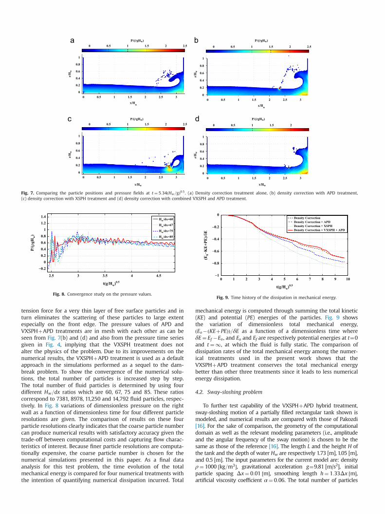
tension force for a very thin layer of free surface particles and inturn eliminates the scattering of these particles to large extentespecially on the front edge. The pressure values of APD andVXSPHþAPD treatments are in mesh with each other as can beseen from Fig. 7(b) and (d) and also from the pressure time seriesgiven in Fig. 4, implying that the VXSPH treatment does notalter the physics of the problem. Due to its improvements on thenumerical results, the VXSPHþAPD treatment is used as a defaultapproach in the simulations performed as a sequel to the dam-break problem. To show the convergence of the numerical solu-tions, the total number of particles is increased step by step.The total number of fluid particles is determined by using fourdifferent Hw=dx ratios which are 60, 67, 75 and 85. These ratioscorrespond to 7381, 8978, 11,250 and 14,792 fluid particles, respec-tively. In Fig. 8 variations of dimensionless pressure on the rightwall as a function of dimensionless time for four different particleresolutions are given. The comparison of results on these fourparticle resolutions clearly indicates that the coarse particle numbercan produce numerical results with satisfactory accuracy given thetrade-off between computational costs and capturing flow charac-teristics of interest. Because finer particle resolutions are computa-tionally expensive, the coarse particle number is chosen for thenumerical simulations presented in this paper. As a final dataanalysis for this test problem, the time evolution of the totalmechanical energy is compared for four numerical treatments withthe intention of quantifying numerical dissipation incurred. Total

mechanical energy is computed through summing the total kinetic(KE) and potential (PE) energies of the particles. Fig. 9 showsthe variation of dimensionless total mechanical energy,ðEo�ðKEþPEÞÞ=δE as a function of a dimensionless time whereδE¼ Ef �Eo, and Eo and Ef are respectively potential energies at t¼0and t ¼1, at which the fluid is fully static. The comparison ofdissipation rates of the total mechanical energy among the numer-ical treatments used in the present work shows that theVXSPHþAPD treatment conserves the total mechanical energybetter than other three treatments since it leads to less numericalenergy dissipation.

4.2. Sway-sloshing problem

To further test capability of the VXSPHþAPD hybrid treatment,sway-sloshing motion of a partially filled rectangular tank shown ismodeled, and numerical results are compared with those of Pakozdi[16]. For the sake of comparison, the geometry of the computationaldomain as well as the relevant modeling parameters (i.e., amplitudeand the angular frequency of the sway motion) is chosen to be thesame as those of the reference [16]. The length L and the height H ofthe tank and the depth of water Hw are respectively 1.73 [m], 1.05 [m],and 0.5 [m]. The input parameters for the current model are: densityρ¼ 1000 ½kg=m3�, gravitational acceleration g¼9.81 [m/s2], initialparticle spacing Δx¼ 0:01 ½m�, smoothing length h¼ 1:33Δx ½m�,artificial viscosity coefficient α¼ 0:06. The total number of particles

Fig. 7. Comparing the particle positions and pressure fields at t ¼ 5:34ðHw=gÞ0:5. (a) Density correction treatment alone, (b) density correction with APD treatment,(c) density correction with XSPH treatment and (d) density correction with combined VXSPH and APD treatment.

2.5 3 3.5 4 4.5

−0.2

0

0.2

0.4

0.6

0.8

1

1.2

1.4

t(g/Hw)0.5

P/(ρ

gHw)

Fig. 8. Convergence study on the pressure values.

0 1 2 3 4 5 6 7 8 9 10−1

−0.8

−0.6

−0.4

−0.2

0

t(g/Hw)0.5

(E0−

KE

+PE

)/δE

Density CorrectionDensity Correction + APDDensity Correction + XSPHDensity Correction + VXSPH + APD

Fig. 9. Time history of the dissipation in mechanical energy.

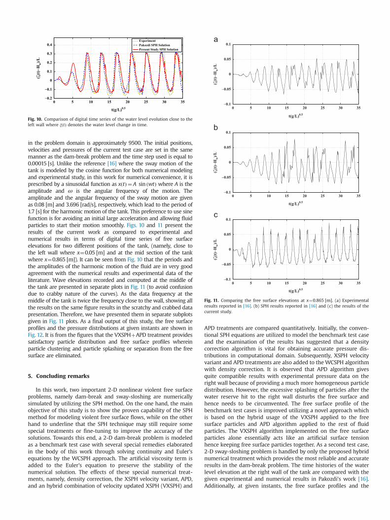
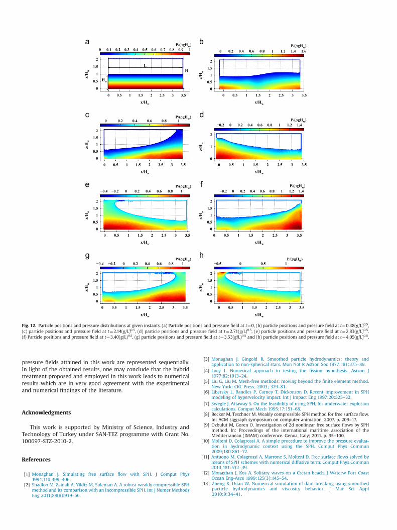
in the problem domain is approximately 9500. The initial positions,velocities and pressures of the current test case are set in the samemanner as the dam-break problem and the time step used is equal to0.00015 [s]. Unlike the reference [16] where the sway motion of thetank is modeled by the cosine function for both numerical modelingand experimental study, in this work for numerical convenience, it isprescribed by a sinusoidal function as xðtÞ ¼ A sin ðwtÞ where A is theamplitude and ω is the angular frequency of the motion. Theamplitude and the angular frequency of the sway motion are givenas 0.08 [m] and 3.696 [rad/s], respectively, which lead to the period of1.7 [s] for the harmonic motion of the tank. This preference to use sinefunction is for avoiding an initial large acceleration and allowing fluidparticles to start their motion smoothly. Figs. 10 and 11 present theresults of the current work as compared to experimental andnumerical results in terms of digital time series of free surfaceelevations for two different positions of the tank, (namely, close tothe left wall where x¼0.05 [m] and at the mid section of the tankwhere x¼0.865 [m]). It can be seen from Fig. 10 that the periods andthe amplitudes of the harmonic motion of the fluid are in very goodagreement with the numerical results and experimental data of theliterature. Wave elevations recorded and computed at the middle ofthe tank are presented in separate plots in Fig. 11 (to avoid confusiondue to crabby nature of the curves). As the data frequency at themiddle of the tank is twice the frequency close to the wall, showing allthe results on the same figure results in the scratchy and crabbed datapresentation. Therefore, we have presented them in separate subplotsgiven in Fig. 11 plots. As a final output of this study, the free surfaceprofiles and the pressure distributions at given instants are shown inFig. 12. It is from the figures that the VXSPHþAPD treatment providessatisfactory particle distribution and free surface profiles whereinparticle clustering and particle splashing or separation from the freesurface are eliminated.

5. Concluding remarks

In this work, two important 2-D nonlinear violent free surfaceproblems, namely dam-break and sway-sloshing are numericallysimulated by utilizing the SPH method. On the one hand, the mainobjective of this study is to show the proven capability of the SPHmethod for modeling violent free surface flows, while on the otherhand to underline that the SPH technique may still require somespecial treatments or fine-tuning to improve the accuracy of thesolutions. Towards this end, a 2-D dam-break problem is modeledas a benchmark test case with several special remedies elaboratedin the body of this work through solving continuity and Euler'sequations by the WCSPH approach. The artificial viscosity term isadded to the Euler's equation to preserve the stability of thenumerical solution. The effects of these special numerical treat-ments, namely, density correction, the XSPH velocity variant, APD,and an hybrid combination of velocity updated XSPH (VXSPH) and

APD treatments are compared quantitatively. Initially, the conven-tional SPH equations are utilized to model the benchmark test caseand the examination of the results has suggested that a densitycorrection algorithm is vital for obtaining accurate pressure dis-tributions in computational domain. Subsequently, XSPH velocityvariant and APD treatments are also added to the WCSPH algorithmwith density correction. It is observed that APD algorithm givesquite compatible results with experimental pressure data on theright wall because of providing a much more homogeneous particledistribution. However, the excessive splashing of particles after thewater reserve hit to the right wall disturbs the free surface andhence needs to be circumvented. The free surface profile of thebenchmark test cases is improved utilizing a novel approach whichis based on the hybrid usage of the VXSPH applied to the freesurface particles and APD algorithm applied to the rest of fluidparticles. The VXSPH algorithm implemented on the free surfaceparticles alone essentially acts like an artificial surface tensionhence keeping free surface particles together. As a second test case,2-D sway-sloshing problem is handled by only the proposed hybridnumerical treatment which provides the most reliable and accurateresults in the dam-break problem. The time histories of the waterlevel elevation at the right wall of the tank are compared with thegiven experimental and numerical results in Pakozdi's work [16].Additionally, at given instants, the free surface profiles and the

0 5 10 15 20 25 30 35−0.2

−0.1

0

0.1

0.2

0.3

0.4

t(g/L)0.5

(ζ(t)

−Hw)/L

ExperimentPakozdi SPH SolutionPresent Study SPH Solution

Fig. 10. Comparison of digital time series of the water level evolution close to theleft wall where ξðtÞ denotes the water level change in time.

0 5 10 15 20 25 30 35−0.1

−0.1

−0.05

−0.05

−0.1

−0.05

0

0.05

0.1

t(g/L)0.5

t(g/L)0.5

t(g/L)0.5

(ζ(t)

−Hw)/L

(ζ(t)

−Hw)/L

(ζ(t)

−Hw)/L

0 5 10 15 20 25 30 35

0

0.05

0.1

0 5 10 15 20 25 30 35

0

0.05

0.1

Fig. 11. Comparing the free surface elevations at x¼0.865 [m]. (a) Experimentalresults reported in [16]. (b) SPH results reported in [16] and (c) the results of thecurrent study.

pressure fields attained in this work are represented sequentially.In light of the obtained results, one may conclude that the hybridtreatment proposed and employed in this work leads to numericalresults which are in very good agreement with the experimentaland numerical findings of the literature.

Acknowledgments

This work is supported by Ministry of Science, Industry andTechnology of Turkey under SAN-TEZ programme with Grant No.100697-STZ-2010-2.

References

[1] Monaghan J. Simulating free surface flow with SPH. J Comput Phys1994;110:399–406.

[2] Shadloo M, Zainali A, Yildiz M, Suleman A. A robust weakly compressible SPHmethod and its comparison with an incompressible SPH. Int J Numer MethodsEng 2011;89(8):939–56.

[3] Monaghan J, Gingold R. Smoothed particle hydrodynamics: theory andapplication to non-spherical stars. Mon Not R Astron Soc 1977;181:375–89.

[4] Lucy L. Numerical approach to testing the fission hypothesis. Astron J1977;82:1013–24.

[5] Liu G, Liu M. Mesh-free methods: moving beyond the finite element method.New York: CRC Press; 2003; 379–81.

[6] Libersky L, Randles P, Carney T, Dickonson D. Recent improvement in SPHmodeling of hypervelocity impact. Int J Impact Eng 1997;20:525–32.

[7] Swegle J, Attaway S. On the feasibility of using SPH, for underwater explosioncalculations. Comput Mech 1995;17:151–68.

[8] Becker M, Teschner M. Weakly compressible SPH method for free surface flow.In: ACM siggraph symposium on computer animation. 2007. p. 209–17.

[9] Ozbulut M, Goren O. Investigation of 2d nonlinear free surface flows by SPHmethod. In: Proceedings of the international maritime association of theMediterranean (IMAM) conference. Genoa, Italy; 2011. p. 95–100.

[10] Molteni D, Colagrossi A. A simple procedure to improve the pressure evalua-tion in hydrodynamic context using the SPH. Comput Phys Commun2009;180:861–72.

[11] Antuono M, Colagrossi A, Marrone S, Molteni D. Free surface flows solved bymeans of SPH schemes with numerical diffusive term. Comput Phys Commun2010;181:532–49.

[12] Monaghan J, Kos A. Solitary waves on a Cretan beach. J Waterw Port CoastOcean Eng-Asce 1999;125(3):145–54.

[13] Zheng X, Duan W. Numerical simulation of dam-breaking using smoothedparticle hydrodynamics and viscosity behavior. J Mar Sci Appl2010;9:34–41.

0 0.5 1 1.5 2 2.5 3 3.5

0

0.5

1

1.5

2

x/Hw x/Hw

x/Hw x/Hw

x/Hw x/Hw

x/Hw x/Hw

z/H

wz/

Hw

z/H

wz/

Hw

z/H

wz/

Hw

z/H

wz/

Hw

0 0.1 0.2 0.3 0.4 0.5 0.6 0.7 0.8 0.9 1

H

Hw

L

P/(ρgHw) P/(ρgHw)

P/(ρgHw)P/(ρgHw)

P/(ρgHw)

P/(ρgHw) P/(ρgHw)

P/(ρgHw)

0 0.5 1 1.5 2 2.5 3 3.50

0.5

1

1.5

2

0 0.2 0.4 0.6 0.8 1 1.2 1.4 1.6

0 0.5 1 1.5 2 2.5 3 3.50

0.5

1

1.5

2

0 0.2 0.4 0.6 0.8 1

0 0.5 1 1.5 2 2.5 3 3.50

1

2

−0.2 0 0.2 0.4 0.6 0.8 1 1.2 1.4

0 0.5 1 1.5 2 2.5 3 3.50

0.5

1

1.5

2

−0.4 −0.2 0 0.2 0.4 0.6 0.8 1

0 0.5 1 1.5 2 2.5 3 3.50

0.5

1

1.5

2

−0.2 0 0.2 0.4 0.6 0.8 1 1.2 1.4

0 0.5 1 1.5 2 2.5 3 3.50

0.5

1

1.5

2

−0.4 −0.2 0 0.2 0.4 0.6 0.8 1

0 0.5 1 1.5 2 2.5 3 3.50

0.5

1

1.5

2

−0.5 0 0.5 1

Fig. 12. Particle positions and pressure distributions at given instants. (a) Particle positions and pressure field at t¼0, (b) particle positions and pressure field at t¼0.38(g/L)0.5,(c) particle positions and pressure field at t¼2.14(g/L)0.5, (d) particle positions and pressure field at t¼2.71(g/L)0.5, (e) particle positions and pressure field at t¼2.83(g/L)0.5.(f) Particle positions and pressure field at t¼3.40(g/L)0.5, (g) particle positions and pressure field at t¼3.53(g/L)0.5 and (h) particle positions and pressure field at t¼4.05(g/L)0.5.

[14] Monaghan J. Smoothed particle hydrodynamics. Rep Prog Phys2005;68:1703–59.

[15] Shadloo M, Zainali A, Sadek H, Yildiz M. Improved incompressible smoothedparticle hydrodynamics method for simulating flow around bluff bodies.Comput Methods Appl Mech Eng 2011;200:1008–20.

[16] Pakozdi C. A smoothed particle hydrodynamics study of two-dimensionalnonlinear sloshing in rectangular tanks [Ph.D. thesis]. Norwegian University ofScience and Technology; 2008.

[17] Cummins S, Rudman M. An SPH projection method. J Comput Phys 1999;152:584–607.

[18] Lee ES, Moulinec C, Xu R, Violeau D, Laurence D, Stancby P. Comparison ofweakly compressible and truly incompressible algorithms for the SPH mesh-free particle method. J Comput Phys 2008;227:8417–36.

[19] Yildiz M, Rook R, Suleman A. SPH with the multiple boundary tangent method.Int J Numer Methods Eng 2009;77:1416–38.

[20] Liu M, Liu G. Smoothed particle hydrodynamics: an overview and recentdevelopments. Arch Comput Methods Eng 2010;17:25–76.

[21] Colagrossi A, Landrini M. Numerical simulation of interfacial flows bysmoothed particle hydrodynamics. J Comput Phys 2003;191:448–75.

[22] Marrone S, Antuono M, Colagrossi A, Colicchio G, Le Touze D, Graziani G. δ-SPH model for simulating violent impact flows. Comput Methods Appl MechEng 2011;200:1526–42.

[23] Dalymple RA, Rogers BD. Numerical modeling of water waves with the SPHmethod. Coast Eng 2006;53:141–7.

[24] Rodriquez P, Bonet J. A corrected smoothed particle hydrodynamics formulationof the shallow water equations. Comput Struct 2005;83:1396–410.