FATIGUE CRACK GROWTH OF CIRCULAR PIPES AND MODELLING …
51
i FATIGUE CRACK GROWTH OF CIRCULAR PIPES AND MODELLING OF SINGLE-EDGE-NOTCH TENSION (SENT) SPECIMEN A THESIS SUBMITTED IN PARTIAL FULFILLMENT OF THE REQUIREMENTS FOR THE DEGREE OF BACHELOR OF TECHNOLOGY IN MECHANICAL ENGINEERING By: SARTHAK SAMBIT SINGH 107ME066 SHANTANU PATNAIK 107ME057 SURAJ TRIPATHY 107ME020 DEPARTMENT OF MECHANICAL ENGINNERING NATIONAL INSTITUTE OF TECHNOLOGY ROURKELA – 769008
Transcript of FATIGUE CRACK GROWTH OF CIRCULAR PIPES AND MODELLING …

i
FATIGUE CRACK GROWTH OF CIRCULAR PIPES
AND MODELLING OF SINGLE-EDGE-NOTCH
TENSION (SENT) SPECIMEN
A THESIS SUBMITTED IN PARTIAL FULFILLMENT OF THE REQUIREMENTS FOR THE DEGREE OF
BACHELOR OF TECHNOLOGY
IN
MECHANICAL ENGINEERING
By:
SARTHAK SAMBIT SINGH 107ME066
SHANTANU PATNAIK 107ME057
SURAJ TRIPATHY 107ME020
DEPARTMENT OF MECHANICAL ENGINNERING
NATIONAL INSTITUTE OF TECHNOLOGY
ROURKELA – 769008

ii
FATIGUE CRACK GROWTH OF CIRCULAR PIPES
AND MODELLING OF SINGLE-EDGE-NOTCH
TENSION (SENT) SPECIMEN
A THESIS SUBMITTED IN PARTIAL FULFILLMENT OF THE
REQUIREMENTS FOR THE DEGREE OF
BACHELOR OF TECHNOLOGY
IN
MECHANICAL ENGINEERING
By:
SARTHAK SAMBIT SINGH 107ME066
SHANTANU PATNAIK 107ME057
SURAJ TRIPATHY 107ME020
Under the guidance of
Prof. P.K.Ray and Prof. B.B.Verma
DEPARTMENT OF MECHANICAL ENGINNERING
NATIONAL INSTITUTE OF TECHNOLOGY
ROURKELA – 769008

iii
NATIONAL INSTITUTE OF TECHNOLOGY
ROURKELA
CERTIFICATE
This is to certify that the thesis entitled “Fatigue Crack Growth of Circular Pipes and
Modeling of Single-Edge-Notched Tension (SENT) Specimen” submitted by Sarthak Sambit
Singh (Roll No. 107ME066), Shantanu Patnaik (Roll No. 107ME057) and Suraj Tripathy
(Roll No. 107ME020) in the partial fulfillment of the requirements for the award of Bachelor
of Technology degree in Mechanical Engineering at National Institute of Technology,
Rourkela (Deemed University) is an authentic work carried out by them under our
supervision and guidance.
To the best of our knowledge, the matter embodied in the thesis has not been submitted to
any other University/Institute for the award of any Degree or Diploma.
Date:
Prof. P.K.Ray Prof. B.B.Verma

iv
ACKNOWLEDGEMENT
We wish to express our deep sense of gratitude and indebtedness to Prof. P.K.Ray,
Department of Mechanical Engineering and Prof. B.B.Verma, Department of Metallurgical
and Materials Engineering, N.I.T Rourkela, for introducing the present topic and for their
inspiring guidance, constructive criticism and valuable suggestion throughout this project
work.
We also extend our sincere thanks to all our friends who have patiently helped us in
accomplishing this undertaking. We also thank Mr. Shashi Kumar and Mr. Pawan Kumar for
their constant support throughout the project work.
Place:
Date:
Sarthak Sambit Singh (107ME066)
Shantanu Patnaik (107ME057)
Suraj Tripathy (107ME020)
Department of Mechanical Engineering
National Institute of Technology
Rourkela - 769008

v
CONTENTS
CHAPTER TITLE PAGE
Certificate iii
Acknowledgement iv
Contents v
List of tables vii
List of figures viii
Abstract ix
1 INTRODUCTION 1-5
1.1 Fatigue 2
1.2 Fracture 3
1.3 Need For Modeling 4
2 LITERATURE REVIEW 6-10
2.1 Circular pipes 7
2.1.1 Assessment of partly circumferential
cracks in pipes
7
2.1.2 Assessment of stress intensity factors in
tubular members
8
2.2 Single edge notched tension (SENT) specimen 8
2.2.1 Assessment of crack growth in SENT
specimen
8
2.2.2 Prediction of fatigue crack growth and
residual life using an exponential model
9
3 EXPERIMENTAL DETAILS 11-17
3.1 Setup and details 12
3.2 Material properties 14
4 FORMULATIONS OF THE MODEL 18-25
4.1 Experimental procedure 19

vi
4.2 Model formulation 25
5 RESULTS AND DISCUSSIONS 26-34
5.1 Results and discussions for circular pipes 27
5.1.1 Data from Instron Machine 27
5.2 Results and discussions for the modeling of SENT
specimen
30
6 CONCLUSION 35-36
6.1 For Circular Pipes 35
6.2 Modeling of SENT Specimen 35
7 REFERENCES 37-38
8 APPENDIX 39-42
8.1 For circular pipes 40
8.2 For modelling of SENT specimen 41
vii
LIST OF TABLES
Sl.
No
Table Name Table
No.
Page
No.
1 Load and Stress Intensity Factor Calculation 3.1 15
2 Chemical Composition of 7020-T7 and 2024-T3 Al
Alloys
4.1 19
3 Mechanical Properties of 7020-T7 and 2024-T3 Al
Alloys
4.2 19
4 Crack Length vs. No. of Cycles for Al 7020-T7 4.3 21
5 Δ K vs. da/dN for Al 7020-T7 4.4 22
6 Crack Length vs. No. of Cycles for Al 2024-T3 4.5 23
7 Δ K vs. da/dN for Al 2024-T3 alloy 4.6 24
8 Results obtained from Instron machine for Pipe 1 5.1 27
9 Results obtained from Instron machine for Pipe 2 5.2 27
10 Values of m for Al 7020-T7 5.3 30
11 Values of ΔK, da/dN and m for Al 7020-T7 5.4 30
12 Values of m for Al 2024-T3 5.5 31
13 Values of ΔK, da/dN and m for Al 2024-T3 5.6 32
14 Values of e for different material 5.7 33

viii
LIST OF FIGURES
Sl. No. Figure Name Fig. No. Page
No.
1 Modes of failure 1.1 4
2 Shear Force and Bending Moment Diagram for
Four Point Bend Test
3.1 12
3 Pre-cracking of specimens 3.2 13
4 Instron 8052 with circular specimen 3.3 16
5 The final cracked circular specimen 3.4 16
6 Instron 8052 with SENT specimen 3.5 17
7 Single edge notched specimen geometry 4.1 20
8 Crack Length vs. No. of Cycles for Al 7020-T7 4.2 21
9 delta K vs. da/dN for Al 7020-T7 4.3 22
10 Crack Length vs No. of Cycles for Al 2024-T3 4.4 23
11 delta K vs. da/dN for Al 2024-T3 alloy 4.5 24
12 a vs. No. of Cycles for pipe 1 5.1 28
13 a vs. ΔK for pipe 1 5.2 28
14 The cross sectional sample as seen under SEM 5.3 29
15 m vs. delta K for Al 7020-T7 alloy 5.4 31
16 m vs. delta K for Al 2024-T3 5.5 32

ix
ABSTRACT
Pipe installations usually experience high amplitude Seismic Vibrations. These vibrations
may initiate a new cracks or it may extend the severity of the exiting cracks. The monitoring
of crack growth and propagation becomes essential if the installation of pipes carry a
hazardous fluid. The compliance technique is one of the most commonly used methods to
measure the crack growth in small size specimen used to monitor crack. Compact tension
(CT), three point bend bar (TPBB) etc. are generally preferred for laboratory tests.
Correlations are available for CT, TPBB and some other geometry of small laboratory
specimens. However, for pipes and elbows no such correlations are available. Fatigue crack
growth tests were carried out on a test specimen in Instron 8502 machine and the necessary
data and graphs were analyzed. Fracture toughness analysis is done with the help of Scanning
Electron Microscope (SEM).
The fatigue crack growth in a body is Exponential in nature. In the second part of this project
a modified gamma model has been proposed to predict the crack growth in a Single Edge
Notched Tension (SENT) Specimen. The values of the different parameters were obtained
and the analysis was done after coding different programs in C++ and MATLAB software.
The final result obtained was found to be coherent with the experimental findings.

CHAPTER 1
INTRODUCTION
FATIGUE
FRACTURE
NEED FOR MODELING CRACK GROWTH

2
1.1 FATIGUE
According to ASTM, Fatigue is defined as “the process of progressive localized permanent
structural change occurring in a material subjected to conditions that produce fluctuating
stresses at some point or points and that may culminate in cracks or complete fracture after a
sufficient number of fluctuations.”[8] The stress value in case of fatigue failure can be less
than ultimate tensile stress and may be below yield stress limit of the material. Generally,
fatigue loading implies to variation of stress and strain in a component in a cyclic manner.
Most of the mechanical components experience fluctuating load due to change in:
Load Magnitude
Load Direction
Load application point
Stages of fatigue failure are [7]:
1. Crack Initiation – It occurs in where there are localized stress concentrations and
geometrical discontinuities are the places where it originates. In such places, the stress
that is induced goes well above the local yield strength of the material.
2. Crack Propagation – Crack propagation occurs along grains or grain boundaries due
to further increase in stress levels. With increase in crack size, cross sectional area
resisting stress decreases.
3. Fracture – The area becomes insufficient to resist induced stress and results in failure
of the component.
Factors that affect fatigue are [7]:
Cyclic stress state: One or more properties of the stress state need to be considered,
depending on the complexity of the geometry and the loading, such as stress
amplitude, mean stress, biaxiality, in-phase or out-of-phase shear stress, and load
sequence.
Geometry: Notches and cross section area variations throughout a body are the places
that have stress concentrations where fatigue cracks initiate.
Surface quality: Surface roughness is the cause of microscopic stress concentrations
and it lowers the fatigue strength

3
Material Type: Fatigue life, as well as the behavior during cyclic loading, varies
from one material to other, e.g. composites and polymers differ significantly from
metals.
Residual stresses: High levels of tensile residual stress can be produced from
Welding, cutting, casting, and other manufacturing processes involving heat or
deformation, which decreases the fatigue strength.
Size and distribution of internal defects: Various casting defects like as gas
porosity, non-metallic inclusions and shrinkage voids significantly reduces fatigue life
of material.
Direction of loading: Fatigue strength also depends on the direction of the principal
stress in non-isotropic materials.
Grain size: Generally smaller grains yield higher fatigue life, but the presence of
various surface defects or scratches will have a higher influence than in a coarse
grained alloy.
Environment: Environmental conditions lead to erosion, corrosion, or gas-phase
embrittlement, which affects the fatigue life of a component.
Temperature: Extreme temperatures can affect and reduce fatigue life of a
component.
1.2 FRACTURE
It is the local separation of an object or material into two or more pieces under action of
stress. They are generally of two types: brittle fracture and ductile fracture.
Brittle Fracture: Here there is no gross plastic deformation before fatigue. Here tensile
stress acts normal to crystallographic plane due to which the fracture occurs by the cleavage.
Ductile fracture: In ductile fracture, before failure, extensive gross plastic deformation takes
place. Here material pulls apart rather than cracking,.

4
Modes of Failure:
There are three modes of crack.
MODE I – It is the opening mode. Here tensile stress acts normal to the plane of crack.
MODE II – Sliding mode where shear stress acts parallel to the plane of crack and
perpendicular to the crack front.
MODE III – Tearing mode where shear stress acts parallel to the plane of crack and parallel
to the crack front.
Fig. 1.1 Modes of Failure
1.3 NEED FOR MODELLING CRACK
Fatigue in material has been studied very closely in past century. 80 to 90 percent of the
failure of materials is due to fatigue. Many infamous accidents like „Versailles train crash‟ in
1848, „de Havilland Comet passenger jets crash‟ in 1954, Alexander L. Kiel land oil platform
capsize in 1980 were caused primarily due to fatigue failure[7]. Hence fatigue life prediction
in components is considered highly important among engineers. Life of a component based
on fatigue consists of two parts:
No. of cycles after which crack initiates
No. of cycles after which crack becomes unstable

5
The initiation of crack can be predicted from stress history and stress analysis but after crack
initiation it becomes difficult to predict the no. of cycles after which the crack becomes
unstable. Practical approach to predict crack is destructive in nature. It is also time consuming
and accurate prediction of crack requires capital as well as skill. Thus to simplify crack
prediction various models like Paris Model, Newman‟s model, Walker FCGR model, Forman
model are proposed. Generally FEM analysis is used to predict crack growth. Here we use an
empirical formula to predict FCGR in a SENT specimen without using complex FEM.

6
CHAPTER 2
LITERATURE REVIEW

7
2.1 CIRCULAR PIPES
2.1.1 ASSESSMENT OF PARTLY CIRCUMFERENTIAL CRACKS IN
PIPES
This part of the project deals in predicting the stress intensity factor of a partly
circumferential elliptical surface crack in pipes. Generally finite element analysis is used
to determine stress intensity factor. Sometimes other approaches like line-spring models
are used for a prediction of crack growth. However, the assessment by FEM is quite
complicated as creation of fine meshes becomes cumbersome in 3D models. The line-
spring element technique proposed by Rice and Levi (1972) [1] provide a simpler
solution but it suffers from issues like correctly estimating Stress Intensity Factor in
complex geometries. There are indirect methods where there is no need to develop a
model that includes a crack. It reduces model development time and degrees of freedom.
Methods like conformal transform (C.D. Wallbrink et al.,2003)[2] can be used to analysis
complex circumferential crack problem and rapidly solves partly circumferential cracks in
pipes. This can be used to solve problems involving non-linear stress distributions. It can
also solve problems involving double curvature, internal cracks quite accurately.
Here two coordinate systems are introduced and are defined as the ω-plane and the z-
plane, respectively. The ω-plane describes the geometry of the (actual) cracks under
investigation in the initial coordinate system. The z-plane basically describes the
geometry where a known solution exists. Here two planes are related by equation
ω = f(z) =ez = re
iθ (2.1)
where, r and θ are coordinates in w-plane.
With this equation the parameters of the problem in the ω-plane are related to those in the
z-plane and by a set of transformations the stress intensity factor is found. The solution
can then be corrected to account for the influence of the boundaries near the crack. Quite
simply the above methodology can be expressed as:
KI =K I ∞
Fρ (2.2)

8
Here K I ∞
is the infinite body solution developed by Vijayakumar and Atluri(1981)[3],
and Fρ is a modification factor used to correct the solution resulting from the inter-actions
of the boundaries around the crack.
2.1.2ASSESSMENT OF STRESS INTENSITY FACTORS IN TUBULAR
MEMBERS.
Stress Intensity Factor at the crack tip is a governing factor that influences fatigue crack
propagation and helps in estimating residual life and criticality of the specimen. FEM
technique uses Stress Intensity Factor for analyzing crack. But there are methods where
crack need not be modeled explicitly ( Peng et. Al) (2003)[5]. Majority of analysis for the
prediction of fatigue cracking is based on line-spring models and finite element models.
Solutions based on line-spring model only concern thin walled structures and do not
consider complex loading while analyzing Stress intensity factors across the crack.
Another approach based on conformal transformation can be used to calculate the Stress
Intensity Factors for 3D cracks under arbitrary loading. But this method cannot be applied
to solve problems that contain axial part through surface cracks. This uses exponential
function to simplify the problem and develops a function to predict crack easily.
2.2 SINGLE EDGE NOTCHED TENSION (SENT) SPECIMEN
2.2.1 ASSESSMENT OF CRACK GROWTH IN SENT SPECIMEN.
Crack prediction in SENT specimen can be done by Finite Element Method as well as by
use of compliance technique. The relationship can be expressed in form of a polynomial
equation (A. Joni et al.,2006)[4]. The coefficients in the polynomial can be calculated
from software like MATLAB. Analytically the coefficients can also be predicted using
FEA software like FRANC2D. The results can be compared to get better crack estimates.
The relationship between compliance (deflection per unit load) and crack length is given
in the form of a polynomial equation and is given by :

9
(2.3)
where, Ci are the compliance coefficients which have to be determined by performing tests
experimentally and also analytically by using FRANC2D and finally the results are
compared. The general formula used in calculation of crack length is:
a/w = C0 + C1U + C2U2 + C3U
3 + C4U
4 + C5U
5 (2.4)
Where C0 , C1 , … are coefficients to be calculated
And U = (1+ (Evb/p) 0.5
)-1
(2.5)
Where, E = Modulus of Elasticity
v = Linear Load Displacement
b = Thickness of Specimen
p = Load Applied
2.2.2 PREDICTION OF FATIGUE CRACK GROWTH AND RESIDUAL
LIFE USING AN EXPONENTIAL MODEL
Earlier various efforts were adopted to correlate and develop relationship between fatigue
crack growth and loading conditions. Mohanty et. al (2009)[6] proposed an exponential
model to predict fatigue crack growth in structures/components subjected to cyclic
loading. It takes into account the change in stress intensity factor which changes with
extension of crack. It uses an equation called law of growth. It has a parameter called
specific growth rate which depends on various loading conditions. Fatigue crack growth
behavior is strongly dependent on initial crack length and load history. The value of
specific crack growth rate, m increases incrementally and depends on two crack driving
forces ΔK and Kmax and material parameters KC, E, σys. The value of specific crack growth
rate depends on a polynomial function of a parameter whose value is determined by
material and loading conditions. The exponential model predicts crack propagation
without complex numerical integration. It is valid for both stage II and stage III of fatigue
crack propagation. The accuracy of the „Exponential model‟ is much better than other
available empirical models and the curves.

10
The general formula is given by :
aj= ai (2.6)
and,
(2.7)
where ai and aj is the crack length in ith step and jth step in mm, respectively; Ni and Nj is
number of cycles in ith step and jth step, respectively; mij is specific growth rate in the interval
i–j; i is the number of experimental steps and j = i + 1.

11
CHAPTER 3
EXPERIMENTAL DETAILS
SETUP AND DETAILS
MATERIAL PROPERTIES

12
3.1 SETUP AND DETAILS
Three straight circular through walled pipes with dimensions given below were considered
for experimental work. The pipe material was preferably SEAMLESS PIPE OF ASTM A 312
TP 316L grades of steel which have in-plane crack growth. The tests were carried out on an
Instron 8502 machine with 250 kN load capacity. The machine was also interfaced to a
computer for control and data acquisition. The tests were conducted in air and in room
temperature. Test on pipe were done by loading it under four point bending. Loading was up
to large scale plastic deformation. The outer circumference of the pipe where the notch was
made was marked by a marker at distance of 0.5mm distance between the markings. Also
there was periodic significant unloading so as to create a beach mark on the crack surface.
After the test, the crack surface was broke open and exact crack length was measured at
various loading stages. The experiments considered in this study were conducted using the
four-point bend method schematically shown in Figure 3.1.
Fig. 3.1 Shear Force and Bending Moment Diagram for Four Point Bend Test
During the test the load was quasi-statically increased under displacement control, until the
maximum load was reached. Because of the low compliance of the test rig, unstable crack
propagation never occurred.

13
The test specimen was gripped between rollers on the INSTRON machine. This type of
loading ensured that the notched section of the pipe was subjected to pure bending stress as
only point contact was on the surfaces of two circles. The pipes with part through and
through-wall notches were fatigue pre-cracked before the fracture tests to ensure sharpness of
the crack tip. The pre-cracking was mainly done using a hack-saw and the wire EDM. This is
shown in Figure 3.2
Fig. 3.2 Pre-Cracking of Specimens
Thereafter fracture tests were carried out on through-wall cracked pipes. The final through-
wall crack size after the fatigue pre-cracking was taken as the initial crack size for the
fracture tests. Pipes were subjected to static loading with a loading displacement rate of
0.036 mm.s-1
. During the test on through-wall cracked pipes, load line displacement (LLD),
load and crack mouth opening displacement (CMOD) were recorded. During the tests on
part-through cracked pipes, the crack depth along the notch length was measured using a
micro gauge based on the principle of alternating current potential difference (ACPD), until
the crack reached through thickness. Thereafter all the parameters measurement required for
through-wall cracked pipe test was carried out. The test was carried out as per the guidelines
of ASTME1820.Here the specimen is unloaded after every 1mm propagation of crack. Here
the amplitude of loading was maintained constant all throughout the test. After certain
number of cycles the pipe broke apart.

14
3.2 MATERIAL PROPERTIES
Tensile tests are done on specimens which were fabricated from the straight pipe. From these
tests, tensile data (e.g. stress-strain diagram, yield stress, UTS, % elongation, % reduction in
area and Young‟s modulus) were determined to be as follows:
UTS = 611.46 MPa
2/3 YS = 241.56 MPa
Also the pipe dimensions were as follows:
Extruded Diameter = 55mm
Outer Diameter (Do) = 60mm
Inner Diameter (Di) = 42mm
Thickness = 8mm
Length = 505mm
Shoulder Length = 53mm
Outer Span = 465mm
Inner Span = 205mm

15
Table 3.1 Load and Stress Intensity Factor Calculation
ΔK ΔP Pmean
25 8.61147 5.2625
30 10.35 6.325
35 12.078 7.381
40 13.797 8.4315
45 15.497 9.47042
50 17.2189 10.5522
55 18.940 11.5749
60 20.662 12.794
65 22.384 13.6794
70 24.1065 14.7317
75 25.8284 15.78403
80 27.5503 16.8363
85 29.2722 17.8885
90 30.9941 18.94084
95 32.716 19.99311
100 34.4379 21.0453
16
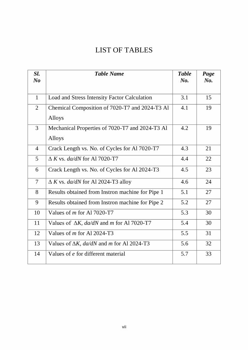
The figure shown here gives us an idea of how the circular pipe specimen is loaded in the
Instron 8502 Machine and the final appearance of the circular pipe specimen after the fatigue
failure.
Fig.3.3 Instron 8052 with circular specimen Fig. 3.4 The final cracked circular specimen

17
The figure shown here gives us an idea of how the circular pipe specimen is loaded in the
Instron 8502 Machine
Fig. 3.5 Instron 8052 with SENT specimen

18
CHAPTER 4
FORMULATIONS OF THE MODEL
EXPERIMENTAL PROCEDURE
MODEL FORMULATION
19
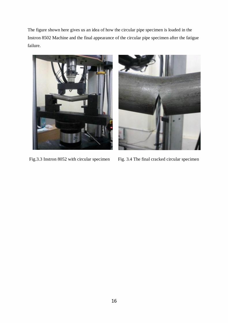
4.1 EXPERIMENTAL PROCEDURE
The present study deals with life prediction model in 7020 and 2024 Al-alloys. The 7020 alloy
was subjected to T7 heat treated condition whereas 2024 alloy was subjected to T3 heat
treated condition in order to obtain optimum mechanical properties. The chemical and
physical properties of the two alloys are given in the tables below:
Table 4.1 Chemical Composition of 7020-T7 and 2024-T3 Al Alloys
Materials Al Cu Mg Mn Fe Si Zn Cr Others
7020-T7 Al-
Alloy
Main
Constituent
0.05 1.2 0.43 0.37 0.22 4.6 - -
2024-T3 Al-
Alloy
90.7-94.7 3.8-4.9 1.2-1.8 0.3-0.9 0.5 0.5 0.25 0.1 0.15
Table 4.2 Mechanical Properties of 7020-T7 and 2024-T3 Al Alloys
Material Tensile
Strength
(σut)
MPa
Yield
Strength
(σys)
MPa
Young’s
Modulus
(E)
MPa
Poisson’s
Ratio
(ν)
Plane Strain
Fracture
Toughness
(K1C)
MPa
Plane Stress
Fracture
Toughness
(KC)
MPa
Elongation
7020-T7
Al-Alloy
352.14 314.7 70000 0.33 50.12 236.8 21.54% in
40mm
2024-T3
Al-Alloy
469 324 73100 0.33 37 95.31 19% in
12.7mm
SENT specimens were used to conduct the experiment. The Fig. 4.1 shows the detailed
geometry of the specimen. The experiments were performed on Instron 8502 machine with
250 kN load cell capacity and which is interfaced to a computer for data acquisition and
control. The tests were conduction in normal atmospheric air and at room temperature. The
test specimens were pre-cracked under mode-I loading to a/w ratio of 0.3. They were then

20
subjected to constant load test with progressive increase in with crack extension,
maintaining a load ratio of 0.1. The load cycles were applied at a frequency of 6 Hz which are
in sinusoidal form. The crack growth was monitored using a crack opening displacement
(COD) gauge mounted on the face of the notch.
Fig 4.1 Single edge notched specimen geometry [4]
The crack length was plotted against the number of cycles the specimen endured. Also the
stress intensity factor range was plotted against the crack growth rate (da/dN). These values
were measured by the COD gauge analyzing the stress level and were interfaced to the
computer to generate us the graphs for the two alloys.[6]

21
For the Al 7020-T7 alloys the graph showing the variation of crack length with the number of
cycles is plotted below:
Fig 4.2 Crack Length vs. No. of Cycles for Al 7020-T7 [6]
From the above graph, the following tables were reconstructed for Al7020-T7 alloys:
Table 4.3 Crack Length vs. No. of Cycles for Al 7020-T7[6]
Number of Cycles N (x 104)
Crack Length (mm)
7.1 18.3
7.6 19.0
8.1 20.0
8.6 20.9
9.1 22.6
9.6 26.4

22
The following graph were plotted for Al 7020-T7 alloys between delta K and da/dN
Fig 4.3 delta K vs. da/dN for Al 7020-T7 [6]
From the above graph, the following tables were reconstructed for Al 7020-T7 alloys:
Table 4.4 delta K vs. da/dN for Al 7020-T7 [6]
Stress Intensity Factor (MPa.m0.5
)
Crack Growth Rate (da/dN) (x 10-4
)
(mm/cycle)
12 1.4
13 2.0
13.2 2.2
14.8 3.0
18.7 7.48

23
For the Al 2024-T3 alloys the graph showing the variation of crack length with the number of
cycles is presented in Fig. 4.3
Fig 4.4 Crack Length vs No. of Cycles for Al 2024-T3 [6]
From the above graph, the following tables were reconstructed for Al 2024-T3 alloys:
Table 4.5 Crack Length vs. No. of Cycles for Al 2024-T3 [6]
Number of Cycles N (x 105)
Crack Length (mm)
0.9 17.75
0.95 18.35
1.0 19.0
1.05 19.75
1.10 20.75
1.15 22.10
1.20 24.45

24
The following graph were plotted for Al 2024-T3 alloys between delta K and da/dN
Fig 4.5 delta K vs. da/dN for Al 2024-T3 alloy [6]
From the above graph, the following tables were reconstructed for Al 2024-T3 alloys
Table 4.6 delta K vs. da/dN for Al 2024-T3 alloy [6]
Stress Intensity Factor ΔK(MPa.m0.5
)
Crack Growth Rate (da/dN) (x 10-4
)
(mm/cycle)
10.2 1.2
10.3 1.3
10.9 1.5
11.7 2.0
12.0 2.2
14.2 4.7

25
4.2 MODEL FORMULATION
Gamma function is a variant of factorial function with its arguments shifted by 1. That is if
„n‟ is a positive integer then:
(4.1)
The Gamma function is defined for every complex number whose real part is positive and
greater than zero. Generally it is given by an integral as mentioned below:
, Re(z) >0 (4.2)
proposed model is a modification of the Gamma function.
Here t can be approximated as number of cycles N. The parameter z was chosen in such a
way that it becomes a non-dimensional parameter yet representing the properties that affect
crack growth.
Here since the integral is finite the value of integral is not Γ(z). The integral was assumed to
be equal to a non-dimensional representing crack growth at the end of fixed cycles of loading.
Generally fatigue crack growth depends on the initial crack length material properties and
dimensions, loading conditions etc. The non-dimensional parameter was chosen to include all
those properties. So the formula for predicting the final crack length at the end of cycle is
given as
=
(4.3)
Here m also a non-dimensional parameter whose value remain approximately constant for a
given cycle interval. At first the value of m on RHS and LHS were considered different say
m1 on LHS and m2 on RHS. The values of a0, w, a1, N were given as input is made fixed for a
particular interval of cycles. The value of m1 is input every time and value of m2 was
computed every time. The value of m1 at which m1 nearly becomes equal to „m2‟ was
considered as the value of m for the interval.
=
. (4.4)

26
CHAPTER 5
RESULTS AND DISCUSSIONS
FOR CIRCULAR PIPES
FOR THE MODELING OF SENT SPECIMEN

27
5.1 RESULTS AND DISCUSSIONS FOR CIRCULAR PIPES
5.1.1 DATA FROM INSTRON MACHINE
Table 5.1 Results obtained from Instron machine for Pipe 1
Length
(curve)
mm
a
(mm)
a/w
ratio
Max.
load(N)
Monitored
Crack
length
(mm)
No. of
Cycles
∆K EVB/P Slope
(x 10-6
)
25.4 2.60 .28 38264 49.46 94195 275.318 569.18 1.2311
28 3.20 0.355 38310 50.92 117679 343.503 630.25 2.5232
34 4.58 0.508 38349 51.53 127741 383.876 692.15 2.7122
38.5 5.96 0.662 38356 52.09 133907 421.47 796.518 2.8311
42 7.05 0.783 38360 52.58 145880 466.66 907.196 3.2231
46 8.39 0.932 38360 53.199 151392 514.76 1080 3.2231
The above results were obtained from the computer interfaced to the Instron 8502 Machine.
Using these values a general curve was plotted to show the variation of crack length with ΔK
and with No. of Cycles, separately.
Table 5.2 Results obtained from Instron machine for Pipe 2
Length
(curve)
(mm)
a(mm) a/w Max.
load
Monitored
Crack
length
(mm)
No. of
Cycles
N
∆K(MPa) EVB/P Slope
(x 10-6
)
27.5 3.096 0.344 38343 51.91 125876 408.722 756.665 2.6762
31.5 4.039 0.44 38304.4 52.33 4510 443.329 845.43 3.0051
35.5 5.096 0.566 38325 52.79 4399 486.89 962.5 3.4395
39.5 6.26 0.696 38304.1 53.28 4193 541.65 1128.32 4.5503
43.5 7.54 0.837 38377 53.71 3241 600.40 1289.31 5.1366
47.5 8.916 0.99 38351.6 54.07 2137 652.55 1452.7 5.737
The above results were obtained from the computer interfaced to the Instron 8502 Machine.

28
Fig. 5.1 a vs. No. of Cycles for pipe 1
Fig. 5.2 a vs. ΔK for pipe 1
0
1
2
3
4
5
6
7
8
9
90000 100000 110000 120000 130000 140000 150000 160000
a( in
mm
)
No. of cycles
0
1
2
3
4
5
6
7
8
9
200 250 300 350 400 450 500 550 600
a (i
n m
m)
ΔK

29
The transverse section of the circular pipe where the crack occurred was taken and viewed
under Scanning Electron Microscope(SEM).Faintly appeared Beach Marks were seen under
fracto--graph.
.
Faintly appeared beach mark
Fig.5.3

30
5.2 RESULTS AND DISCUSSIONS FOR THE MODELING OF SENT
SPECIMEN
The following tables were constructed for Al 7020-T7 alloys:
Table 5.3 Values of m for Al 7020-T7
No. of
Cycles(104)
Crack
Length
(mm)
m in
Simpson’s
1/3 rule
‘m1’ from
MATLAB
m2 from
MATLAB
7.1 18.3
7.6 19.0 10.248 10.249 10.253
8.1 20.0 9.9143 9.912 9.91
8.6 21.1 9.3963 9.436 9.429
9.1 22.6 9.0893 8.976 8.975
9.6 26.34 8.610 8.601 8.604
Table 5.4 Values of delta K, da/dN and m for Al 7020-T7
Crack Growth Rate (da/dN)
(x 10-4
) (mm/cycle)
Stress Intensity Factor
(MPa.m0.5
)
The values of m from the
empirical relation
1.4 12 10.21
2.0 13 9.91
2.2 13.2 9.85
3.0 14.8 9.43
7.48 18.7 8.82

31
The following trends were observed when the graph was plotted for „m-model‟ and
„m-experimental‟ with delta K for Al 7020-T7 alloy:
Fig 5.4 m vs. delta K for Al 7020-T7 alloy
Similarly the following tables were constructed for Al 2024-T3 alloys:
Table 5.5 Values of m for Al 2024-T3
No. of
Cycles(105)
Crack
Length
(mm)
‘m1’ from
MATLAB
‘m2’ from
MATLAB
0.9 17.75
0.95 18.35 10.551 10.551
1.0 19.0 10.211 10.211
1.05 19.75 9.876 9.876
1.10 20.75 9.532 9.532
1.15 22.10 9.112 9.112
1.20 24.45 8.657 8.657

32
Table 5.6 Values of delta K, da/dN and m for Al 2024-T3
Crack Growth Rate (da/dN)
(x 10-4
) (mm/cycle)
Stress Intensity Factor
(MPa.m0.5
)
The values of m from the
empirical relation
1.2 10.2 9.87
1.3 10.3 9.84
1.5 10.9 9.6
2.0 11.7 9.33
2.2 12.0 9.21
4.7 14.2 8.57
The following trends were observed when the graph was plotted for m-model and
m-experimental with delta K for Al 2024-T3 alloy:
Fig 5.5 m vs. delta K for Al 2024-T3
From the above two tables the value of „m‟ is found to have a reducing trend in both cases.
The value of m reduces with increase in the value of ΔK. The value of m changes with change

33
in loading condition as well as crack length. Hence it was needed to correlate parameter m
with parameters like two crack driving forces ΔK and Kmax and with the material parameters
such as plane stress fracture toughness (KC), modulus of elasticity (E) and yield stress (σys).
Fatigue crack growth depends on both ΔK and Kmax in order to consider effects of mean
stress. Since the modeling covers region III the value of fracture toughness (KC) has to be
considered. Crack growth also depends upon the material parameters like yield stress (σys) ,
Young‟s Modulus (E) and Ultimate strength (σut) . The parameter „m‟ is dimensionless and
has a decreasing trend. So the value of m is correlated with dimensionless quantities like (E/
σys), (KC / ΔK), (Kmin /Kmax).
The resulting value of m is represented as:
(5.1)
Here the value of exponent e varies from one material to other. The values of e for both the
specimens used in the model are given below:
Table 5.7 Values of e for different material
Material Exponent e
7020-T7 Al Alloy 0.382
2024-T3 Al Alloy 0.428
The value of e for each case as shown is different hence it must depend on certain properties
which vary from one specimen to other. After some permutations it was found that the value
of e depends upon the material parameters like ultimate strength (σut) and the Young‟s (E) of
the material. It was found that the ratio of the values of e depends upon the ratio:

34
(5.2)
The values of e were compared and calculated. It was found that the value of e satisfies
following formula:
(5.3)
Where C= Constant
Comparing this formula with the values of exponents in each case it was found that the value
of e is approximately equals to:
(5.4)

35
CHAPTER 6
CONCLUSION
FOR CIRCULAR PIPES
MODELING OF SENT SPECIMEN

36
6.1 FOR CIRCULAR PIPES
1. From Fig. 5.1, it was observed that the crack growth rate increases very sluggishly initially
with the no. of cycles but after that the crack growth rate increase at a faster rate.
2. From Fig. 5.1,it was observed that the crack growth rate increases very sluggishly initially
with Δ K but after that the crack growth rate increase at a faster rate.
3. The transverse section of the circular pipe where the crack occurred was cut by means of a
hand milling machine. It was cut in such a way that crack surface is not hampered. This
section is then viewed under Scanning Electron Microscope (SEM) in order to see the pattern
of Beach Marks. But no prominent beach marks were seen in the fracto-graph. The reason for
this might be due to the fact that the specimen was subjected to constant amplitude loading
with the growth/propagation of the crack. The possibility of the appearance of beach marks
would have been more prominent if the specimen would have been subjected to increasing
amplitude loading with the growth/propagation of the crack after every unloading.
6.2 MODELING OF SENT SPECIMEN
1. The Modified Gamma Model of the form,
=
(6.1)
is used for predicting the fatigue life of a component without going for the numerical
integration. This formula holds good in the region II and region III of the fatigue life curve.
The results obtained from the Modified Gamma Model are in good agreement with the
experimental results for the SENT specimen. The variation is primarily due to experimental
errors or other errors arising due faulty reading and human error. This method can be
extended to circular pipes and elbows. The value of „m’ can be modified for use in prediction
of crack for other non standard specimens. This method is easy to interpret and less time
consuming in successfully predicting crack with good degree of accuracy.
2. There are many other method and models like Weibull Model, Beta Model that can be
modified and adopted for predicting crack growth for different specimen

37
CHAPTER 7
REFERENCES

38
[1] Rice, J.R. and Levy, N. (1972). The part-through surface crack in an elastic plate. Journal of
Applied Mechanics, Transactions ASME, 185–194.
[2] Wallbrink C.D., Peng D. and Jones R. (2003). Assessment of partly circumferential
cracks in pipes. International Journal of Fracture (2005): 167-181
[3] Vijayakumar, K. and Atluri, S.N. (1981). Embedded elliptical crack, in an infinite
solid, subject to arbitrary crack-face tractions. Journal of Applied Mechanics,
Transactions ASME 48, 88–96.
[4] Mohanty J.R. , Joni A. , Ray P.K. , Verma B.B. (2006). Determination of crack
coefficients for a single edge-notch tension specimen using franc2d program. Recent
trends in mechatronics, nanotechnology and robotics RTMNR(2006),742-746
[5] Peng D., Wallbrink C., Jones R. (2004). An assessment of stress intensity factors for
surface flaws in a tubular member. Engineering Fracture Mechanics Volume 72, Issue
3, February 2005, 357-371
[6] Mohanty J.R., Ray P.K. , Verma B.B. (2008). Prediction of fatigue crack growth and
residual life using an exponential model: Part I (constant amplitude loading).
International Journal of Fatigue Volume 31, Issue 3, March 2009, Pages 418-424
[7] Wikipedia, May 02 2011. < http://en.wikipedia.org/wiki/Fatigue_(material)>
[8] Stephens, Ralph I.; Fuchs, Henry O. (2001). Metal Fatigue in Engineering (Second
edition ed.). John Wiley & Sons, Inc.. p. 69.

39
CHAPTER 8

40
APPENDIX
8.1 FOR CIRCULAR PIPES
In order to feed data to the INSTRON machine, via the computer, some calculations were
done. A sample calculation is done below:
Assuming Stress Intensity Factor ΔK = 30 MPa and Range R=0.1
Now, we know that ΔK = Δσ * (π*R*θ)1/2
* F(θ)
where F(θ) = 1 + 6.8 (θ/π)3/2
– 13.6(θ/π)5/2
+ 20(θ/π)7/2
Now here 2θ = 900 or θ=45
0
Therefore, θ/π = 0.25 or F(θ) = 1.5812
Radius R = 21 x 10-3
m
Therefore, Δσ = 83.58 MPa
But Δσ = σmax – σmin = σmax (1-R) = 0.9 σmax
Or σmax = 92.86 Mpa
I = π/64 (Do4 - Di
4) and a = (465-205)/2 = 130 mm
y = D0/2
Now
or
or P = 0.115 x 10⁵ N = 11.5 kN
Pmin = Pmax * R = 1.15 kN
ΔP = 10.35 KN and Pmean = 6.325 kN

41
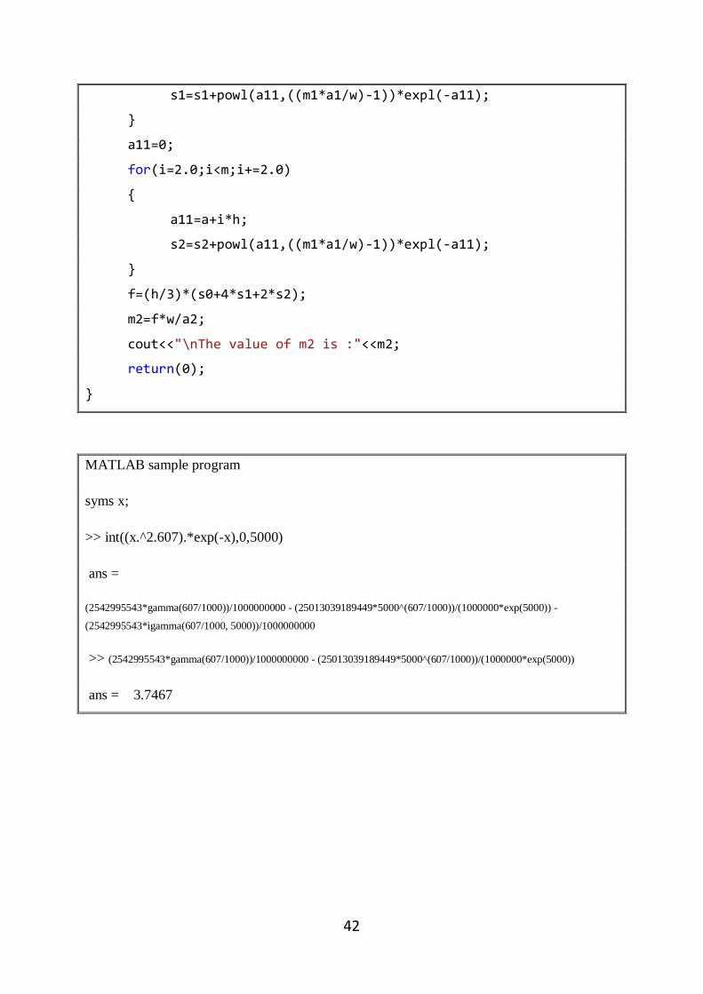
8.2 For Modeling of SENT Specimen
The value was computed with the help of software MATLAB as well as C++ where
Simpson‟s 1/3 Rule was applied whose code is given in the table below.
//Program to calculate value of ‘m’
#include<iostream>
#include<conio.h>
#include<math.h>
using namespace std;
int main()
{
long double a1,w,m1,m2,a2,a,b,h,f,s0,s1,s2,a11;
long double i,m;
a1=18.3; //initial crack length
a2=19.0; //final crack length
a=0.0;
b=5000; //number of cycles
w=52.00; //value of width
cout<<"\nEnter the value of m1 :";
cin>>m1; //Value of m1
m=10000000;
h=(b-a)/m;
s1=0;
s2=0;
//Simpson's 1/3 rule computation
s0=powl(a,((m1*a1/w)-1))*expl(-a)+powl(b,((m1*a1/w)-1))*expl(-
b);
for (i=1.0;i<m;i+=2.0)
{
a11=a+i*h;
42
s1=s1+powl(a11,((m1*a1/w)-1))*expl(-a11);
}
a11=0;
for(i=2.0;i<m;i+=2.0)
{
a11=a+i*h;
s2=s2+powl(a11,((m1*a1/w)-1))*expl(-a11);
}
f=(h/3)*(s0+4*s1+2*s2);
m2=f*w/a2;
cout<<"\nThe value of m2 is :"<<m2;
return(0);
}
MATLAB sample program
syms x;
>> int((x.^2.607).*exp(-x),0,5000)
ans =
(2542995543*gamma(607/1000))/1000000000 - (25013039189449*5000^(607/1000))/(1000000*exp(5000)) -
(2542995543*igamma(607/1000, 5000))/1000000000
>> (2542995543*gamma(607/1000))/1000000000 - (25013039189449*5000^(607/1000))/(1000000*exp(5000))
ans = 3.7467