STATE HIGHWAY ADMINISTRATION

RESEARCH REPORT

EXPERIMENTAL INVESTIGATIONS ON MECHANICAL BEHAVIOR OF UNSATURATED SUBGRADE SOIL WITH

LIME STABILIZATION AND FIBER REINFORCEMENT

NATIONAL TRANSPORTATION CENTER MORGAN STATE UNIVERSITY

SP107B4J FINAL REPORT

November 2003

MD-03-SP107B4J

Robert L. Ehrlich, Jr., Governor Michael S. Steele, Lt. Governor

Robert L. Flanagan, Secretary Neil J. Pedersen, Administrator

The contents of this report reflect the views of the author who is responsible for the facts and the accuracy of the data presented herein. The contents do not necessarily reflect the official views or policies of the Maryland State Highway Administration. This report does not constitute a standard, specification, or regulation.

Experimental Investigations on Mechanical Behavior of Unsaturated Subgrade Soil with Lime Stabilization and Fiber Reinforcement

By Jiang Li, PhD., P.E. Associate Professor

Room 220, MEB Department of Civil Engineering

School of Engineering Phone: 443.885.4202

Fax: 443.885.8218 Email: jli@eng.morgan.edu

Morgan State University 5200 Perring Parkway Baltimore, MD 21251

November 2003

3

1. Report No.

MD-03-SP107B4J 2. Government Accession No. 3. Recipient's Catalog No.

5. Report Date November 2003

4. Title and Subtitle

Experimental Investigations on Mechanical Behavior of Unsaturated Subgrade Soil with Lime Stabilization and Fiber Reinforce

6. Performing Organization Code

7. Author/s Dr. Jiang Li

8. Performing Organization Report No.

10. Work Unit No. (TRAIS)

9. Performing Organization Name and Address Morgan State University 1700 E. Cold Spring Lane Baltimore, MD 21251-0001

11. Contract or Grant No. SP107B4J

13. Type of Report and Period Covered Final Report

12. Sponsoring Organization Name and Address Maryland State Highway Administration Office of Policy and Research 707 North Calvert Street Baltimore MD 21202

14. Sponsoring Agency Code

15. Supplementary Notes 16. Abstract In the present report, experimental investigations on mechanical behavior of unsaturated subgrade soil with fiber reinforcement and lime stabilization were conducted. The soil samples were collected from the soil/aggregate laboratory at the Maryland State Highway Administration (MD-SHA), Maryland Department of Transportation. The experiments were carried out to investigate physical and mechanical properties of subgrade soil that was mixed with geofiber and lime. The reinforced and stabilized soil with fiber and lime is considered as a composite material. Investigations in this study included two phases. In the first phase, the investigation was for static behavior of composite subgrade soil under the compressive shear loading. In the second phase, the investigation emphasized dynamic behavior of reinforced and stabilized soil under cyclic shear loading. In this research, three aspects of investigations are presented. First, new constitutive models for static and dynamic loading were established for composite material. In the present report, elastic constitutive relationship was assumed to describe both the linear and nonlinear shear stress-strain relations of composite material. Static behavior was described with a nonlinear elastic model, and dynamic behavior was expressed with a linear elastic model. For the nonlinear model, elastic shear modulus was assumed to be a function of multiple variables such as shearstrain, contents of fiber and lime, confining pressure, and the curing period of samples. In contrast, for the linear model, elastic modulus was not only defined as a function of confining pressure, contents of fiber and lime, and the aging period of samples but also repetitions of cyclic loading. For convenience ofexperimental investigation, the shear stress-strain relation in a three-dimensional stress space reduced to that in a quasi-triaxial stress space in which the conventional triaxial shear tests were conducted. Second, experimental investigations and calibration of constitutive models were conducted.

4

Experimental data from laboratory tests were utilized to verify and justify the linear or nonlinear elastic model suggested in this report. Constitutive parameters of linear and nonlinear models were investigated and calibrated using experimental results from both static and dynamic triaxial shear tests. The linear regression method was adopted to find constitutive parameters. The constitutive relationship of the composite material made of soil, fiber and lime was established once constitutive parameters for the linear and nonlinear models were determined. The elastic shear moduli were investigated, for example, the initial shear and tangential moduli in the nonlinear elastic model under static loading, and the shear or resilient modulus in the linear model under cyclic loading. Moreover, for static loading, the Coulomb –Mohr’s failure criterion was applied. The strength indices c and φ were studied for the composite soil with fiber and lime. A linear relation was introduced to describe parameters c and φ as a function of fiber and lime content, and the sample-curing period. The coefficients of the linear relation for parameters c and φversus fiber and lime content, and sample aging time were found using the experimental data. Finally, impacts of fiber and lime as well as other factors that affect mechanical behavior of the composite material were discussed. Impact factors on shear moduli were introduced for both the linear and nonlinear models. The impact factors for the nonlinear model under static loading were defined to exhibit effect of variables such as cell pressure, fiber and lime contents, and the sample-curing period on the initial modulus and soil strength, namely parameters 1/A and 1/B related to the shear modulus G. In contrast, the impact factors for the linear model under cyclic loading were introduced to show effect of the same variables (σ0, mF, mL and t) plus the repetition of cyclic loading on resilient modulus and dynamic behavior of composite soils. 17. Key Words Constitutive Relationship, Nonlinearity, Shear Stress and Strain, Deviatoric Stress and Strain, Elastic Modulus, Resilient Modulus, Fiber Reinforcement, Lime Stabilization, Composite Material

18. Distribution Statement: No restrictions This document is available from the Research Division upon request.

19. Security Classification (of this report) None

20. Security Classification (of this page) None

21. No. Of Pages 97

22. Price

Form DOT F 1700.7 (8-72) Reproduction of form and completed page is authorized.

5

TABLE OF CONTENTS

ABSTRACT....................................................................................................................... 4 ACKNOWLEDGMENTS ................................................................................................ 6 INTRODUCTION............................................................................................................. 7 CONSTITUTIVE RELATIONSHIP .............................................................................. 8

Elastic Stress – Strain Relationship in a Three Dimensional Space ......................... 8 Elastic Stress – Strain Relationship in a Quasi Three Dimensional Space .............. 9 The Linear Elastic Stress – Strain Relation .............................................................. 10 The Nonlinear Elastic Stress – Strain Relation......................................................... 11

EXPERIMENTAL INVESTIGATIONS...................................................................... 14 Specimen Preparation ................................................................................................. 14

Materials applied and tested ................................................................................... 14 The procedure for specimen preparation .............................................................. 14

Equipment and Test Conditions................................................................................. 15 The device and testing conditions for static tests .................................................. 15 The device and testing conditions for dynamic tests............................................. 15

Test Results and Data Analysis .................................................................................. 16 Mechanical behavior in response to static loading................................................ 16

Results of static compressive shear tests ............................................................... 16 Parameter calibration for the nonlinear model .................................................... 20 Tangential shear modulus Gt of the composite material under static loading .... 21 Impact factors IAi and IBi for parameters A and B in the nonlinear model......... 22 Failure of composite material under static shear stress ....................................... 23

Mechanical behavior in response to dynamic loading .......................................... 24 Results of cyclic shear tests.................................................................................... 25 Parameter calibration for the linear model .......................................................... 27 Resilient modulus Mr of the composite material under cyclic loading ............... 28 Impact factors IGi on shear modulus G in the linear model................................. 28 Failure of composite material under cyclic shear stress ...................................... 29

SUMMARIES AND CONCLUSIONS.......................................................................... 30 NOMENCLATURE........................................................................................................ 33 REFERENCES................................................................................................................ 35 THE LIST OF FIGURES............................................................................................... 37

Figure 1 Hyperbolic stress – strain relationship....................................................... 37 Figure 2 The linear relation used to determine A and B ......................................... 38 Figure 3 ( 1σ − 3σ ) vs. ε1 with mL = 0%, and different mF and σ0 .......................... 39 Figure 4 ( 1σ − 3σ ) vs. ε1 with mF = 0.2%, mL = 5% and different σ0 and t.......... 40

Figure 5 ( 1σ − 3σ ) vs 1. ε with mF = 0.5%, mL = 5% and different σ0 and t .......... 41

Figure 6 1ε /( 1σ − 3σ ) vs 1. ε with mL = 0% and different mF and σ0 ...................... 42

Figure 7 1ε /( 1σ − 3σ ) vs 1. ε with mF = 0.2%, mL = 5% and different σ0 and t ...... 43

Figure 8 1ε /( 1σ − 3σ ) vs 1. ε with mF = 0.5%, mL = 5% and different σ0 and t .... 44 Figure 9 ( 1σ − 3 σ ) vs. 1ε with mL = 0%, and different mF and σ0 .......................... 45

1

Figure 10 ( 1σ − 3σ ) vs. 1 εσ

with mF = 0.2%, mL = 5%, and different σ0 and t ...... 46 Figure 11 ( 1 − 3σ ) vs. 1ε with mF = 0.5%, mL = 5%, and different σ0 and t ...... 47

Figure 12 1ε /( 1 − 3 ) vs. 1σ σ ε with mL = 0%, and different mF and σ0..................... 48 Figure13a ( 1σ − 3 ) vs. 1 with mσ ε

σε

.

L = 5%, t = 7 days, and different mF and σ0..... 49 Figure13b ( 1 − 3 ) vs. 1ε with mσ L = 5%, t = 14 days, and different mF and σ0 .. 50 Figure13c ( 1σ − 3 ) vs. 1σ with mL = 5%, t = 28 days, and different mF and σ0... 51

Figure14a 1 /( 1 − 3 ) vs 1ε σ σ ε with mL = 5%, t = 7 days, and different mF and σ0 . 52

Figure14b 1 /( 1 − 3 ) vs 1ε σ σ . ε with mL = 5%, t = 14 days, and different mF and σ0 53

Figure14c 1ε /( 1 − 3 ) vs 1σ σ . ε with mL = 5%, t = 28 days, and different mF and σ0 54 Figure 15 Mohr’s circles with mL = 0% and different mF ....................................... 55 Figure 16 Mohr’s circles with mL = 5% and mF= 0.2% and different t ................. 56 Figure 17 Mohr’s circles with mL = 5%, mF = 0.5% and different t ...................... 57 Figure 18 Cohesion c vs. fiber content mF and curing time t .................................. 58 Figure 19 Friction angle φ vs. fiber content mF and curing time t .......................... 59 Figure 20 σd ~εd with mL=2%, mF= 0.2%, t =7 days, and different σ0 and N........ 60 Figure 21 σd ~εd with mL=5%, mF= 0.2%, t =7 days, and different σ0 and N........ 61 Figure 22 σd ~εd with mL=5%, mF= 0%, t =7 days, and different σ0 and N........... 62 Figure 23 σd ~εd with mL=2%, mF= 0.5%, t =7 days, and different σ0 and N........ 63 Figure 24 σd ~εd with mL=2%, mF= 0.2%, t=7 days, and different σ0 and N......... 64 Figure 25 σd ~εd with mL=5%, mF= 0.5%, t =7 days, and different σ0 and N........ 65 Figure 26 σd ~εd with mL=2%, mF= 0%, t =14 days, and different σ0 and N......... 66 Figure 27 σd ~εd with mL=2%, mF= 0.2%, t =14 days, and different σ0 and N...... 67 Figure 28 σd ~εd with mL=5%, mF= 0.2%, t =14 days, and different σ0 and N...... 68 Figure 29 σd ~εd with mL=2%, mF= 0.5%, t =14 days, and different σ0 and N...... 69 Figure 30 σd ~εd with mL=5%, mF= 0.5%, t =14 days, and different σ0 and N...... 70 Figure 31 σd ~εd with mL=2%, mF= 0%, t =28 days, and different σ0 and N......... 71 Figure 32 σd ~εd with mL=2%, mF= 0.2%, t =28 days, and different σ0 and N...... 72 Figure 33 σd ~εd with mL=5%, mF= 0.2%, t =28 days, and different σ0 and N...... 73 Figure 34 σd ~εd with mL=0%, mF= 0.2%, t =28 days, and different σ0 and N...... 74 Figure 35 σd ~εd with mL=2%, mF= 0.5%, t =28 days, and different σ0 and N...... 75 Figure 36 σd ~εd with mL=5%, mF= 0.5%, t =28 days, and different σ0 and N...... 76 Figure 37 G vs. N, mL, mF, t and σ0 ............................................................................ 77 Figure 38 Mr ~σm with t =7 days and different mF, mL and N................................ 78 Figure 39 Mr ~σm with t =14 days and different mF, mL and N.............................. 79 Figure 40 Mr ~σm with t =28 days and different mF, mL and N.............................. 80

THE LIST OF TABLES................................................................................................. 81 Table 1 Specimens for static tests with fiber and without lime............................... 81 Table 2 Specimens for static tests with fiber and lime ............................................. 82 Table 3 Specimens for dynamic tests with mF = 0% and mL = 2% ......................... 83 Table 4 Specimens for dynamic tests with mF = 0% and mL = 5% ......................... 84 Table 5 Specimens for dynamic tests with mL = 0%, and mF = 0.2 & 0.5% .......... 85 Table 6 Specimens for dynamic tests with mF = 0.2% and mL = 2% ...................... 86

2

Table 7 Specimens for dynamic tests with mF = 0.5% and mL = 5% ...................... 87 Table 8 Specimens for dynamic tests with mF = 0.2% and mL = 5% ...................... 88 Table 9 Specimens for dynamic tests with mF = 0.2% and mL = 2% ...................... 89 Table 10 A and B values from static shear tests ....................................................... 90 Table 11 Calibration of parameters and coefficients ai, bi and ci............................ 91 Table 12 Strength indices c and φ with different mF, mL and t ............................... 92 Table 13 Shear modulus G with mF = 0%, mL = 5%, different σ0, N and t............ 93 Table 14 Shear modulus G with mF = 0.2%, mL = 2%, different σ0, N and t......... 94 Table 15 Shear modulus G with mF = 0.5%, mL = 5%, different σ0, N and t......... 95 Table 16 Shear modulus G with mF = 0.2%, mL = 5%, different σ0, N and t......... 96 Table 17 Shear modulus G with mF = 0.5%, mL = 2%, different σ0, N and t......... 97

3

ABSTRACT In the present report, experimental investigations on mechanical behavior of unsaturated subgrade soil with fiber reinforcement and lime stabilization were conducted. The soil samples were collected from the soil/aggregate laboratory at the Maryland State Highway Administration (MD-SHA), Maryland Department of Transportation. The experiments were carried out to investigate physical and mechanical properties of subgrade soil that was mixed with geofiber and lime. The reinforced and stabilized soil with fiber and lime is considered as a composite material. Investigations in this study included two phases. In the first phase, the investigation was for studies of static behavior of composite subgrade soil under the compressive shear loading. In the second phase, the investigation emphasized dynamic behavior of reinforced and stabilized soil under cyclic shear loading. In this research, three aspects of investigations were presented. First, new constitutive models for static and dynamic loading were established for the composite material. In the present report, elastic constitutive relationship was assumed to describe both the linear and nonlinear shear stress-strain relations of the composite material. Static behavior was described with a nonlinear elastic model, and dynamic behavior was expressed with a linear elastic model. For the nonlinear model, elastic shear modulus was assumed to be a function of multiple variables such as shear strain, contents of fiber and lime, confining pressure, and the curing period of samples. In contrast, for the linear model, elastic modulus was not only defined as a function of confining pressure, contents of fiber and lime, and the aging period of samples but also repetitions of cyclic loading. For convenience of experimental investigation, the shear stress-strain relation in a three-dimensional stress space reduced to that in a quasi-triaxial stress space in which the conventional triaxial shear tests were conducted. Second, experimental investigations and calibration of constitutive models were conducted. Experimental data from laboratory tests were utilized to verify and justify the linear or nonlinear elastic model suggested in this report. Constitutive parameters of linear and nonlinear models were investigated and calibrated using experimental results from both static and dynamic triaxial shear tests. The linear regression method was adopted to find constitutive parameters. The constitutive relationship of the composite material made of soil, fiber and lime was established once constitutive parameters for the linear and nonlinear models were determined. The elastic shear moduli were investigated, for example, the initial shear and tangential moduli in the nonlinear elastic model under static loading and the shear or resilient modulus in the linear model under cyclic loading. Moreover, for static loading, the Coulomb – Mohr’s failure criterion was applied. The strength indices c and φ were studied for the composite soil with fiber and lime. A linear relation was introduced to describe parameters c and φ as a function of fiber and lime contents, and the sample-curing period. The coefficients of the linear relation for parameters c and φ versus fiber and lime contents, and the sample aging time were found using the experimental data. Finally, impacts of fiber and lime as well as other factors that affect mechanical behavior of the composite material were discussed. Impact factors on shear moduli were introduced for both the linear and nonlinear models. The impact factors for the nonlinear model under static loading were defined to exhibit effect of variables such as cell pressure, fiber and lime contents, and the sample-curing period on the initial modulus and

4

soil strength, namely parameters 1/A and 1/B related to the shear modulus G. In contrast, the impact factors for the linear model under cyclic loading were introduced to show effect of the same variables (σ0, mF, mL and t) plus the repetition of cyclic loading on resilient modulus and dynamic behavior of composite soils.

5

ACKNOWLEDGMENTS This two-year research program was sponsored by the Maryland State Highway Administration (MD -SHA) and the National Transportation Center (NTC) at Morgan State University (MSU). The principal investigator (the P.I.) is grateful to both the MD-SHA and the NTC-MSU for their support in this research project.

6

INTRODUCTION One of the top priorities of highway administrations is to increase productivity and decrease the rate of road wear [1]. Improvement of the nation's highways performance is normally focused on the quality of the roadway surface. Pavement performance will largely rely on the mechanical behavior of pavement and subgrade soil layers. In order to increase the capacity of transportation of highway systems, it is recommended to use the higher payload of trucks to improve road productivity as the higher payload reduces both the total number of vehicles in operations and the cost of truck freight transport that is about $140 billon per annum (TPA, 1985). The higher payload, however, increases the rate of road deterioration due to a higher level of shear stress within pavement and subgrade layers. The higher level of shear stress induced by traffic loads not only affects performance of the road surface but also impacts interaction between pavement and subgrade soil layers. Therefore, it is important to investigate the composite subgrade soil with better mechanical properties that can improve road quality under the vehicle-induced shear force. In this present investigation, subgrade soil mixed with fiber and lime powder is utilized for shear testing because geofiber contributes extra tensile and shear resistance to reinforce subgrade soil, and lime provides additional binding and cohesive force to stabilize subgrade soil. Geofiber is one of many geosynthetic products and is widely used in Geotechnical Engineering to improve engineering properties of materials. For example, soil material with fiber reinforcement improves material strength against tensile and shear stress so that risk of pavement cracking and rutting is lowered. The advantages of using the geofiber material reinforcement are many such as low cost, lightweight, convenient construction and transportation, strong anti-biologic erosion, high chemical stabilization, etc. If lime (CaO) is also added to composite subgrade soil, the effect of interlock, shear and tensile resistance can be enhanced. Although many investigators previously conducted research for soils reinforced with geofiber [2-12], little effort has been made for composite subgrade soil reinforced with both geofiber and lime powder. The present research centers on investigating mechanical behavior of subgrade soil mixed with fiber and lime in response to the both static and dynamic loads. For static tests, there are three aspects. First, nine groups of triaxial shear tests have been conducted with three different groups of specimens that are sample soil mixed with fiber only and with both fiber and lime. The sample soil with different fiber and lime contents is cured for a period prior to triaxial shear tests. Second, a nonlinear elastic model is introduced to describe nonlinear elastic behavior of unsaturated subgrade soil with lime stabilization and fiber reinforcement. Third, constitutive parameters of this model are investigated and calibrated using experimental results from conventional triaxial shear tests. In contrast, dynamic tests are carried out for experimental investigations on cyclic behavior of the fiber-reinforced and lime-stabilized soil. The experimental investigations were conducted using dynamic triaxial apparatus. Test data and results from dynamic shear tests were collected and analyzed to determine how composite soil responds to cyclic loading and how mechanical properties of subgrade soil can be improved. It should be pointed out that research findings and results from the present investigations not only can be utilized for design in roadbeds but also can be employed for other applications such as improvement of soft ground, stabilization of soil slops, and reinforcement of bridge footings, shallow and deep foundations in highway engineering.

7

CONSTITUTIVE RELATIONSHIP The constitutive relationship of deformable material represents the physical law describing the relation between stress and strain. In the present report, the elastic constitutive relationship for the composite soil is introduced and studied. Elastic Stress – Strain Relationship in a Three Dimensional Space

The elastic stress – strain relation can be linear and nonlinear, and is defined below [13]:

klijklij E εσ = , (Eq.1) or can be expressed in terms of volume and shear stress-strain relations by:

Dijijkk

Dijijkkij G23 ε+δκε=σ+δσ=σ (Eq.2)

where σij

σ

= a stress tensor (kPa) = the trace of the stress tensor (kPa) kk

σD = a shear stress tensor (kPa) ij

εkl = a strain tensor εk = the trace of the strain tensor when k = 1, 2 and 3 are repeated. k

δ = the Kronecker delta (δ =1 when i = j; δ = 0 when i ≠ j; i and j = 1, 2, and 3) ij ii ij

κ = bulk modulus, a parameter of elasticity (kPa) G = shear modulus, a parameter of elasticity (kPa)

ijkl = the fourth order tensor of elasticity (kPa), and is defined byE :

jlikjkilklijijkl

)(G)3/G2(E δδ+δδ+δδ−κ=

ns: in Eq.2 can be lternatively expressed in terms of stress and strain invariants [14]:

(Eq.3) The volume and shear stress-strain relatio D

ijDijkkkk G2and3 ε=σκε=σ

a

D2

D211 J2GIandJ3κI == (Eq.4a, 4b)

where

I = σkk = (σ11 + σ22 + σ33), the first invariant of a stress tensor (kPa) 1

J1 = εkk = (ε11 + ε22 + ε33), the first invariant of a strain tensor

8

ID = D , the second invariant of a deviatoric stress tensor (kPa).

e following five elastic parameters, namely, arameter λ, bulk modulus κ, shear modulus G, Poisson’s ratio ν, and Young’s modulus

e three-dimensional ace needs to reduce to a quasi-triaxial space in which the conventional triaxial shear sts are conducted. For instance, in the principal quasi-triaxial stress space, σ1 ≠ σ2 = σ3,

ε1 lat ns in q.4a a 4b re

(Eq.4c)

here (σ1-σ3) is difference of the major and minor principal stresses σ1 and σ3; (ε1- ε3) is ifference of the major and minor principal strains ε and ε . For conventional triaxial

sh

ay not play a role in causing the nonlinearity of stress-stain relationship. he present investigation emphasizes the shear stress-strain relation shown in Eq.4e. oth the linear and nonlinear shear stress-strain relations are introduced and discussed in e next section.

2/σσ D2 ijij

JD2 = /2εε D

ijDij , the second invariant of a deviatoric strain tensor.

The elastic stress-strain relation for isotropic, homogenous and isothermal material can be described using any two out of thpE. It should be pointed out that throughout this report, stresses, if not specified, are effective stresses rather than total stresses. Elastic Stress – Strain Relationship in a Quasi Three Dimensional Space

For convenience of experimental investigations, stress and strain in th

spte

≠ ε2 = ε3, and the stress-strain re io E nd duce to:

)2(32 3131 ε+εκ=σ+σ

)(G2 3131 ε−ε=σ−σ (Eq.4d) wd 1 3

ear tests, Eq.4d can be further simplified to:

131 G2 ε=σ−σ (Eq.4e) Eq.4e represents the axial deviatoric stress-strain relation that was studied and verified via shear tests using the conventional triaxial apparatus in laboratory. It should be pointed out that in Eqs.4c and 4d, both the bulk and shear moduli κ and G are functions of multiple variables that are to be discussed in the next section. The variables related to strain, stress, or rates of strain and stress may have significantly impacts on shear modulus G, and cause the nonlinearity of stress-strain relationship in Eq.4e. In contrast, the variables associated with the materials such as fiber, lime, etc. may also affect shear

odulus G but mmTBth

9

The Linear Elastic Stress – Strain Relation

In this report, a linear elastic model is introduced for the dynamic stress-strain relation. This suggests that all strain is instantaneously and totally recoverable upon the removal of the loaded stress. Stress increases proportionally or linearly with increase of strain. The elastic modulus in the linear model is not a function of strain though it can be a

nction of other variables related to the composite material. In this report, for example, ulk and shear moduli are defined by:

κ (Eq.5)

(Eq.6)

where loading (N is an integer and N≥1).

specimens prior to shear tests (day)

tion in Eq.4e is applied. The shear odulus G in Eq.6 is assumed to be a product of multiples power functions of five

ariables [14], and is given in the following form:

c )t/t()N()m, + (Eq.7)

nless. ubstituting Eq.7 into Eq.4b gives the linear shear stress-strain relation written in terms

in the three dimensional stress space:

fub

)t,N,m,m,I( lf1κ=

G )t,N,lf1= m,m,I(G

I1 = σkk, the first invaria= c

nt of stress (kPa). N repetitions of cyclit = the curing period of mF = fiber content (%) mL = lime content (%)

Fiber and lime contents mF and mL within prepared soil specimens are defined by WF/(WS + WL) and WL/WS respectively. WF, WL and WS stand for weights of fiber, lime powder and dry soil. In research of dynamic behavior under cyclic loading, investigating shear modulus G n Eq.6 is focused if the shear stress-strain relai

mv

54321 c

1cc

LcG F010LF1 1()m1()p/I(c)t,N,mm,I( +=

here pw 0 = unit atmospheric pressure (kPa) t1 = one day (day) ci (i = 0 …5) = constitutive coefficients that are dimensionless except for c0 (kPa)

he terms pT 0 and t1 in Eq.7 are introduced to make ratios σ0/p0 and t/t1 dimensioSof invariants of shear stress and strain tensors

D2

c1

ccL

cF

c010

D2 J)(t/t(N))m(1)m(1)/p(IcI 54321 ++= (Eq.8a)

10

If the quasi-triaxial stress space is applied for experimenta Eq.4e, Eq.8a reduces to:

us ε1 in Eq.8b represents a family of the linear elastic relations. However, if e shear modulus G of elasticity is a function of the axial shear strain or stress, then the

. In the next section, the nonlinear elastic under static loads will be introduced and

is

ge. For e nonlinear elastic model, elastic parameters κ and G are a function of variables such as

train, strain rate, time and other variables. For example, the bulk modulus κ and shear modulus G can be defined as a function of the first and the second deviatoric invariants of

and JD1 that are related to volume and shear strains individually:

LF11= (Eq.9)

J1 and JD2 are related to volume and

hear strains respectively. Therefore, for the nonlinear stress–strain model, elastic stress ose not change linearly with elastic strain. As mentioned previously, research of the

l investigations, then according to

1c

1cc

Lc

Fc

0003154321 )t/t()N()m1()m1()p/(c ε++σ=σ−σ (Eq.8b)

where σ0 simplified from I1 is confining or cell pressure (kPa), and the coefficient 2 in Eq.4e is dropped and included in the parameter c0 in Eq.8b One may note that in Eq.7 shear modulus G of elasticity is not a function of shear strain. Therefore, when testing conditions and material parameters (i.e., σ0, N, t, mF and mL) are given, G becomes a constant and the relation (σ1- σ3) versus ε1 in Eq.8b is the linear elastic relation. For different values of variables σ0, N, t, mF and mL, the relation (σ1- σ3) versthshear stress-strain relation becomes nonlinear

tress-strain relation model describing the sd cussed. The Nonlinear Elastic Stress – Strain Relation

For the static investigations, a nonlinear elastic model is suggested to express the

stress-strain relation of subgrade soil. Soil as one of many engineering materials exhibits evident nonlinear mechanical behavior particularly when soil deformation is larths

strain tensors J1

κ t),m,m,J,κ(I

t),m,m,J,G(IG LF

D21= (Eq.10)

Comparing to the linear model in Eqs.5 and 6, one may notice that in Eqs.9 and 10 both bulk and shear moduli are functions of strain tensor invariants J1 and JD

2 but not cyclic loading repetition N. The strain invariantssdshear stress-strain relation in q.4e emphasized. Moreover, the shear modulus G in Eq.10 is defined in the following expression [15]:

E is

)JB1/(AG D

2+= (Eq.11)

11

where A and B (1/kPa) are constitutive xpressions in the quasi-triaxial space:

++= (Eq.12a)

here ai and bi (i = 1…4) are constitutive parameters and are to be determined using the xperimental data from the static triaxial shear tests. Bearing Eqs.12a and 12b in mind

and inserting Eq.11 into Eq.4b yield the shear stress-strain relation in terms of invariants of stress and strain tensors:

parameters, and defined by the following e

4321 a1

aL

aF

a000 )(t/t)m(1)m(1)/p(σaA

4321 b

1b

Lb

Fb

000 )(t/t)m(1)m(1)/p(σbB ++= (Eq.12b) we

D2

1LF

00

1LF

00 J])

t()m(1)m(1)

p([b])

t()m(1)m(1)

p([a 43214321 +++++

bbbb1aaaa1

D2D

2 tItIJ

I =

(Eq.13)

which can further reduce to a simplified form in the quasi triaxial stress space according

to Eq.4e:

1b

1

bL

bF

b

0

00

a

1

aL

aF

a

0

00

131

]ε)tt()m(1)m(1)

pσ

([b])tt()m(1)m(1)

pσ

(a[

ε

43214321 +++++=−σσ

(Eq.14)

where the coefficient 2 in Eq.4e, similar to the linear model, is dropped and included in

impact f confining pressure on the stress-strain relation is not considered, then Eq.14 further is implified to the nonlinear hyperbolic model first introduced by Konder [17]. In the

present investigation, the expression Eq.14, the generaliz d hyp rbolicstrain model for the composite subgrade soil, is introduced to describe the nonlinear ehavior of the composite soil under static loading. In order to understand the hyperbolic relation given by Eq.14, it is worthy to discuss

the parameters a0 and b0 in Eq.14 for convenience of discussion. If material parameters mL and mF equal zero (i.e., sample soil without fiber and lime), then Eq.14 reduces to the nonlinear model presented by Duncan et al. [16]. If theos

e e elastic stress–

b the physical meaning of parameters defined in Eq.14. For constant parameters A and B defined in Eqs.12a and 12b, one can rewrite Eq.14 by the following simple form:

12

11

131 )BA

1(G εε+

=ε=σ−σ (Eq.15)

In

ngent modulus fact, from the stress-strain relation shown in Figure 1, parameters A and B are

tively the reciprocal of the initial ta Gi (1/kPa) [ = (σ1-σ3)/ε1|ε→0

1/A] and the reciprocal of the asymptotic or ultimate value of the stress difference (σ1-

(Eq.16)

Apparently, parameters A and of a straight line. If experimental results from the static triaxial compressive tests support

e relation shown in Eq.16, then the nonlinear model in Eq.15 is justified and verified as ell.

respec=σ3)ult [=(σ1-σ3)|ε→∞ = 1/B] (see Figure 2). From Eq.15, the following linear relation between 1/G [=ε1/(σ1-σ3)] and the axial strain ε1 should be addressed as it is useful when the constitutive parameters are to be determined from the experimental data, namely:

BεA)σ/(σε1/G +=−= 1311

B shown in Figure 2 represent the intercept and the slope

thw Accordingly, the tangential modulus Gt (= d(σ1-σ3)/dε1) can be derived by taking derivative of Eq.15 with respect to the axial strain ε1:

211

31t )BA(

A)( σ−σ∂G

ε+=

ε∂= (Eq.17)

The physical meaning of the tangential modulus Gt is also shown in Figure 1. As parameters A and B in Eq. 12a and 12 b are functions of multiple variables (i.e., σ0, t, mF and mL), Eq.17, therefore, represents a family of curves. This is true for the relations in Eqs.15 and 16 as well. The constitutive parameters in both the linear and nonlinear models are to be calibrated from the experimental investigations in the next section.

13

EXPERIMENTAL INVESTIGATIONS Specimen Preparation Materials applied and tested Sample soils for tests were taken from the Soil/Aggregate Laboratory at the Geotechnical Exploration Division at the Maryland State Highway Administration (SHA). These subgrade soils were originally collected from road construction sites in Howard Country, Maryland and had the following physical properties: the wet unit weight γdry = 17 kN/m3

(95 lb./ft3); plastic limit PL = 5%; the soil classification (AASHTO) is A4. Lime powder used for specimen preparations was manufactured by the Lhoist Group Company. The lime powder is made of chemical hydrated lime with high calcium. The employed lime powder comprises Calcium Oxide (>71.5%) and Magnesium Oxide (about 1.0%). 100 percent of lime powder particles can pass through No. 20 U. S. standard sieve and 93% through No. 100 US. standard sieve. The product of lime powder meets the standards of American Water Works Association (AWWA B202 – 93) for the hydrated lime. Geofiber used for specimen preparation was manufactured by Synthetic Industries Inc. The fiber is made of polypropylene, a chemically stable and inert polymer. The fibers mixed with sample soil are flexible, black and discrete strands about 3.5 cm (about 1.5 in) in length. Specimens for both static and dynamic shear tests were prepared with fiber contents mF = 0%, 0.2% and 0.5% and lime contents mL = 0%, 2% and 5% by weight, respectively.

The procedure for specimen preparation Sample preparation for conventional triaxial shear tests follows the procedure suggested by Synthetic Industries Inc.: 1. Soil Processing. Process soils through a #4 sieve; then thoroughly mix sample. Split

sample into appropriate batches, not to exceed 10 lbs. (4.5 kg.) 2. Soil Conditioning. Place soil sample in mixing bowl. Start mixer and slowly add the

required moisture to bring the sample up to approximately 80% of optimum moisture. Mix the soil sample until water is well distributed throughout the batch, based on visual observation. Remove moist soil and seal in plastic bag for 24 hours to allow specimen to hydrate thoroughly.

3. Mixing Procedure. Mixer bowl should not be filled more than one-half full for mixing. Therefore, weigh up to 10 lbs. (4.5 kg.) of soil into the mixer bowel. Add enough water to bring this batch to optimum moisture content. Uniformly spread the soil batch in 5 equal depth lifts in the mixer bowl, adding the fibers on each lift as described below. Uniformly spread ¼ of the total fiber content for the batch over the first lift of soil. Place the second lift of soil over the first layer of fibers. Continue this soil-fiber sequence until all the soil and fibers have been added. There will be 5 lifts of soil and 4 lifts of fibers, so the 5th lift of soil will cover the 4th lift of fibers and

14

no fibers will be visible at the surface prior to mixing. Mix the batch while at the same time, adding the remaining water. The water must be added slowly so that a continuous stream is supplied to the batch. Placing all the water too soon or intermittent adding of the water will result in a poor-mixing operation. The entire batch should have received an initial mixing operation by the time the final water is added. Mix until the mixture appears uniform. Remove the soil from the mixer bowl, place the mixture into bags and seal. Let the mixture hydrate for at least 24 hours prior to preparation of test specimens.

4. Sample Remold. The remolded mixture sample is compacted using a compaction mold (7.12 cm D x 14.2 cm H). Compact a specimen in five layers. Weigh 1,500 g mixture sample and separate it into five, so each layer has an equal amount of mixture. Each layer is compacted with 15 blows using a 2.5 kg. rammer. Trim both upper and lower surfaces. Remove the mold, keep the sample in a plastic bag to avoid loss of water content and place the specimen in a water bath until it is ready for the triaxial test. The specimen is cylindrical with a dimension of 6.86 cm (2.8 inch) in diameter and 13.72 cm (5.6 inch) in height.

5. Sample curing. Before shear tests, three aging periods (7, 14 and 28 days) are respectively used to cure the specimens with lime powder. During the curing periods, room humidity and temperature are controlled to minimize the moisture loss of the prepared specimens that are put in the sealed plastic bags.

Equipment and Test Conditions The device and testing conditions for static tests Experimental investigations for static shear tests were conducted using the triaxial shear apparatus manufactured by GEOCOMP Corp. The static triaxial apparatus has a strain-control system. The strain rate of compressive shear tests was 0.6% per minute. The axial mono-increase loading exerted on top of a specimen was controlled at a constant strain rate till the specimen failure occurs. Testing data such as axial stress and strain were collected through transducers by a data acquisition system. The value of the strength or the stress at failure was determined by taking either the peak stress value or the stress value at the axial strain = 15%. The shearing tests followed the AASHTO code T297 (or ASTM D4767) with the consolidation-undrained (CU) condition. Confining or cell pressures applied for triaxial shear tests were 50, 100, 150, or 200 kPa, respectively. The shear tests were conducted for specimens with different curing periods, different contents of fiber and lime. Specimens are prepared with mL = 0%, 2% and 5% and mF = 0%, 0.2% and 0.5%. The group number of tested specimens and experimental conditions applied to triaxial static shear tests were listed in Tables 1 and 2. The device and testing conditions for dynamic tests Experimental investigations for dynamic tests were conducted using a dynamic triaxial compressive shear test apparatus (RMT-1000). The RMT1000 system is the stress control shear device, and is manufactured by Structured Behavior Engineering Laboratory, Inc. Similar to static shear tests, cyclic shear tests were conducted under different testing conditions (e.g., different cyclic repetitions and confining pressures) for several groups of specimens having three curing periods, and two contents of fiber and

15

lime. The specimens are the same as those prepared for static shear tests, namely three lime contents (mL = 0%, 2% and 5%) and three fiber contents (mF = 0%, 0.2%, and 0.5%) except four confining or cell pressures for dynamic triaxial shear tests are 21, 50, 100 or 150 kPa, respectively. Cyclic repetitions for loading N are 50, 100 and 500. The axial cyclic loading waveform has a half-sine form. Shear tests are carried out by following the AASHTO code T292-91 with the CU condition. The axial load and deformation of the specimen, etc. are measured during the loading procedure. The tested specimen named and experimental conditions applied to triaxial cyclic shear tests are listed in Tables 3–9. The specimen n Tables 3 - 9 are named by the following way: 21, A, B and C in the first one or two letter represent the cell pressures 21, 50, 100 or 150 kPa respectively; the following two letters 07, 14 and 28 stands for the curing periods; then the next two letters indicate fiber and lime contents (e.g., 52 stands for mF = 0.5 % and mL = 2 %) and the last three letter are for the cyclic repetition N (i.e., 50, 100 or 150). The sample number 21145250, for example, denotes the specimen with σ0 = 21 kPa, t = 14, mF = 0.5%, mL = 2% and N = 50. Similarly, the sample number A0755100 stands for σ0 = 50 kPa, t = 7 days, mF = 0.5%, mL = 5% and N = 100. Test Results and Data Analysis Mechanical behavior in response to static loading Research in this section is focused on investigating impacts of fiber and lime on the stress-strain relations as well as strength of composite soil under static loading. As mentioned in the early section, the stress-strain relation in response to the triaxial shear force is studied using the nonlinear elastic model introduced in Eq.15. This nonlinear model has two functions A and B. Each of functions A and B with constitutive parameters (ai and bi, i = 0…4) is defined as a product of four power functions for variables mF, mL, σ0 and t. The constitutive parameters are to be determined by applying the experimental data from the compressive shearing tests that are discussed in details below. Results of static compressive shear tests Various results from more than thirty-six shear tests are collected, processed and presented through Figure 3 to Figure 19. Based on shear tests, effects of multiple variables on mechanical behavior of composite soil are analyzed and discussed respectively as follows: 1. Impacts of cell pressure and fiber content on the stress-strain relation without lime. Relations (σ1 − σ3) versus ε1 (the deviatoric stress versus the axial strain) are presented in Figures 3a, 3b and 3c for cell pressure σ0 = 50, 100, 150 and 200 kPa. Each figure corresponds to fiber contents mF = 0%, 0.2% and 0.5% and mL = 0% (i.e., the specimens without lime). The impact of cell pressure and fiber content on the stress-strain relation is evident. For example, the family curves in each figure indicate effect of cell pressure on the stress-strain relation as stress increases with increase of confining pressure for any given strain. Furthermore, the effect of fiber content mF on the strength of composite

16

subgrade soil can be observed by picking up one curve from each figure with the same cell pressure. If the relations (σ1 − σ3) versus. ε1 with cell pressure σ0 = 50 kPa are chosen from Figures 3a, 3b and 3c, for instance, the axial stress values (σ1 − σ3) at the axial strain ε1 = 5% are 90, 120, and 150 kPa which respectively correspond to mF = 0%, 0.2% and 0.5 %. The fiber impact on soil strength is also demonstrated in Figures 9a, 9b and 9c for the later discussion. As the tested specimens in this group have no lime content, for the given cell pressure shear strength increases due to the fiber reinforcement In all three figures, the relations of (σ1 − σ3) versus ε1 are nonlinear. The axial deviatoric stress (σ1 − σ3) nonlinearly changes with the axial strain ε1. Moreover, based on the testing data the relations 1/G = ε1/(σ1 − σ3) versus ε1 with the same testing conditions are drawn in Figures 6a, 6b and 6c that correspond to Figures 3a, 3b and 3c individually. Test curves in Figures 6a, 6b and 6c illustrate that the relation ε1/(σ1 − σ3) versus ε1 is linear, and that parameters A and B as assumed in Eqs.12 and 13 are functions of variables mF, mL and σ0 since the slope B and intersection A of the straight lines shown in Figures 6a, 6b and 6c change with variables. This also suggests that the assumption of the nonlinear model in Eq.15 can be confirmed by the testing results because the linear relation Eq.16 with parameters A and B is an alternative expression of the hyperbolic relation Eq.15.

2. Impacts of cell pressure and sample-curing time on the stress-strain relation with both fiber and lime.

Nonlinear relations (σ1 − σ3) versus ε1 are shown in Figures 4a, 4b and 4c for cell pressures σ0 = 50, 100, and 150 kPa and fiber contents mF = 0.2% and lime content mL = 5%. For each figure, the curing period t is 7, 14 and 28 days individually. For given mF = 0.2% and mL = 5%, impacts of cell pressure and the specimen-curing periods on the stress-strain relation are noticeable. Namely, with increase of cell pressure the axial stress increases at any given axial strain ε1. Effect of specimen curing time on the stress-strain relation can be observed by selecting one curve with given cell pressure from each diagram from Figures 4a, 4b and 4c. For instance, choosing the curve with cell pressure σ0 = 50 kPa from the family curves in Figures 4a, 4b and 4c finds that stress values at the axial strain ε1 = 5% are individually 480, 600, and 800 kPa and correspond to t = 7, 14 and 28 days. More explicit exhibition of effect of the specimen-aging period on the stress-strain relation is shown and discussed in the later section. Similarly, relations between (σ1 − σ3) and ε1 shown in Figures 4a, 4b and 4c are nonlinear, and the axial deviatoric stress (σ1 − σ3) increases with increase of axial strain ε1. The linear expressions 1/G = ε1/(σ1 − σ3) versus ε1 from the samples in the same group are plotted in Figures 7a, 7b and 7c that are associated with Figures 4a, 4b and 4c respectively. The linear relations between 1/G = ε1/(σ1 − σ3) versus ε1 in Figures 7a, 7b and 7c support the nonlinear relation in Eq.16 in which parameters A and B are not only functions of mF, mL and σ0 but also functions of the sample-curing period t.

17

3. Impacts of cell pressure and the sample-curing time on the stress-strain relation with both fiber and lime.

Nonlinear relations (σ1 − σ3) versus ε1 shown in Figures 5a, 5b and 5c are similar to those shown in Figures 4a, and 4c except for mF = 0.5% rather than 0.2%. For the given mF = 0.5% and mL = 5%, impacts of cell pressure and the specimen-curing periods on the stress-strain relation are obvious. Namely, with increase of cell pressure σ0 the axial stress (σ1 − σ3) increases at any given axial strain ε1. The effect of the specimen-curing time on the stress-strain relation can be observed by selecting one curve with given cell pressure from each figures. For instance, picking the curve with cell pressure σ0 = 50 kPa from the family curves in Figures 5a, 5b and 5c finds that the stress values at the axial strain ε1 = 5% are 600, 800, and 1000 kPa and correspond to t = 7, 14 and 28 days individually. This suggests that soil shear strength increases with the specimen-aging time so that elastic shear modulus G is a function of the sample-curing period t as assumed in Eq.10. The axial deviatoric stress (σ1 − σ3) nonlinearly increases with the axial strain ε1 as well. The linear expression 1/G = ε1/(σ1 − σ3) versus ε1 plotted in Figures 8a, 8b and 8c are related to Figures 5a, 5b and 5c. Again, from Figures 8a, 8b and 8c, the linear relation between 1/G = ε1/(σ1 − σ3) and ε1 confirms the nonlinear model in Eq.16, and the expressions for parameters A(mF, mL, σ0 and t) and B(mF, mL, σ0 and t) in Eqs.12a and 12b. 4. Impacts of cell pressure and fiber on the stress-strain relation without lime (mL = 0%). Family curves of relations (σ1 − σ3) vs. ε1 in Figures 9a, 9b and 9c are in response to fiber contents mF = 0%, 0.2% and 0.5 % and lime content mL = 0% (i.e., specimens without lime stabilization). The stress-strain relations for three family curves are plotted in Figures 9a, 9b and 9c for cell pressures σ0 = 50, 100, and 150 kPa individually. Figures 9a, 9b and 9c demonstrate impacts of fiber reinforcement (mF = 0%, 0.2% and 0.5 %) on soil strength. Each stress-strain relation in the family curves in Figures 9a, 9b and 9c increases with the fiber content. For each stress-strain relation, the axial deviatoric stress (σ1 − σ3) increases nonlinearly with increase of axial strain ε1. This supports the assumption that the elastic shear modulus G (related to parameters A and B) is a function of fiber content mF as defined by Eq.10. The linear expressions 1/G = ε1/(σ1 − σ3) versus ε1 related Figures 9a, 9b and 9c are plotted in Figures 12a, 12b and 12c. As mentioned in the previous discussion, the linear expression in Figures 12a, 12b and 12c allows one to determine parameters A and B conveniently. At the same time, based on the test data, the linear relation between 1/G = ε1/(σ1 − σ3) and ε1 justifies the nonlinear model in Eq.14 and the linear expression in Eq.16. 5. Impacts of the sample curing period and cell pressure on the stress-strain relation with

given fiber and lime

The family curves of relations (σ1 − σ3) vs. ε1 in Figures 10a, 10b, 10c and 10d are in response to three sample-curing periods (t = 7, 14, and 28 days). The four figures with mF = 0.5% and mL = 5% are correspondingly plotted with cell pressures σ0 = 50, 100, 150, and 200 kPa. Figures 10a, 10b, 10c and 10d are alternative illustrations of Figures

18

4a, 4b and 4c, and exhibit impacts of the sample-curing periods (t = 7, 14 and 28 days) on the stress-strain relations. Each stress-strain curve of the family curves in Figures 10a, 10b, 10c and 10d nonlinearly increases with the sample-curing time. For each stress-strain relation, the axial deviatoric stress (σ1 − σ3) increases nonlinearly with axial strain ε1. This verifies that soil shear strength increases with the specimen-aging time, and elastic shear modulus G is a function of the sample-curing period t introduced in Eq.10. In fact, one also can draw the linear relation between ε1/(σ1 − σ3) and ε1 for the different sample-curing periods to determine parameters A and B.

6. Impacts of the sample-curing periods and cell pressure on the stress-strain relation

with given contents of fiber and lime. The family curves for relations (σ1 − σ3) versus ε1 in Figures 11a, 11b and 11c are drawn with three different sample-curing periods (t = 7, 14, and 28 days). Three figure with mF

= 0.2%, mL = 5% are individually plotted with cell pressure σ0 = 50, 100, and 150 kPa. The same attempt is made to demonstrate impacts of the sample-curing periods (t = 7, 14 and 28 days) on the stress-strain relations. Each stress-strain relation in the family curves shown in Figures 11a, 11b and 11c increases with the sample-curing time. For each stress-strain relation, the axial deviatoric stress (σ1 − σ3) increases nonlinearly with increase of the axial strain ε1. This validates the elastic shear modulus G in Eq.10 as a function of the sample-curing period t in this group with specific conditions.

7. Impacts of fiber content and cell pressure on the stress-strain relation with lime. More curves in Figures 13a, 13b and 13c with the parameter mF are illustrated for impacts of fiber content, cell pressures and the curing periods on the stress-strain relation. For instance, Figures 13a1, 13a2 and 13a3 indicate the fiber effect (mF = 0.2% and 0.5%) on the stress-strain relation (σ1 − σ3) vs. ε1 with increased cell pressure σ0 = 50, 100, or 150 kPa, lime content mL = 5% and the curing period t = 7days. In contrast, Figures 13b1, 13b2 and 13b3 are plotted to demonstrate the fiber effect on the axial stress-train relations with the same conditions except for the curing period t = 14 days. Figures 13b1, 13b2 and 13b3 are also to illustrate the fiber effect on the axial stress-train relations with the curing period t = 28 days instead. Similar to the previous discussion, the axial stress in Figures 13a, 13b and 13c increases with increase of fiber content at any given axial strain. The stress-strain relations in Figures 13a and 13b and 13c are nonlinear and suggest the elastic modulus is the function of the axial strain. For purpose of comparison, Figures 14a, 14b and 14c corresponding to Figures 13 a, 13b and 13c are plotted to show the linearity between ε1/(σ1 − σ3) and ε1 so that the functions A and B and related parameters in the nonlinear model can be determined.

8. Impacts of fiber reinforcement on soil strength without lime stabilization. Figures 15a, 15b and 15c show effect of fiber reinforcement (mF = 0.0, 0.2, and 0.5%) on the Column-Mohr’s failure line with mL = 0% and at ε1f = 15% where ε1f is the axial strain at failure. The relations of cohesion c and friction angle φ versus fiber content mF found from Figures 15a, 15b and 15c are linear and drawn in Figures 18a and 19a respectively. From Figures 18a and 19a, the fiber reinforcement plays a significant role

19

in strength of composite soil because the strength parameter c and φ show linear relations with fiber content mF. 9. Impacts of the sample-curing periods on the soil strength with lime stabilization. Figures 16a, 16b and 16c show the effect of the sample-curing time t (7, 14 and 28 days) on the Column-Mohr’s failure line with mF = 0.2%, mL = 5% and ε1f = 15%. From Figures 16a, 16b and 16c, the relations of cohesion c and friction angle φ versus the aging time t are drawn in Figures 18b and 19b respectively. From Figures 18b and 19b, strength indices c and φ increase linearly with the curing period t. Impact of sample curing periods on the soil strength can also be found with the identical conditions except for mF = 0.5% from Figures 17a, 17b and 17c in which effect of the sample-curing time t on the Column-Mohr’s failure line is obvious (mL = 5% and ε1f = 15%). In the same way, Figures 18c and 19c indicate that strength indices c and φ linearly increase with the sample-aging time (mF = 0.5% and mL = 5%). In future sections, impacts of fiber and lime reinforcement will be discussed in details. In brief, experimental results from the static triaxial shear tests verify the nonlinear stress-strain model in Eq.15 and shear modulus G in Eq.16 with various combinations of four variables σ0, mF, mL and t having different values, indicate effects of the four variables on soil static behavior such as the stress-strain relation and soil failure, provide the necessary information for calibration of the ten constitutive coefficients, and finally suggest the linear relation of the strength parameters c and φ have linear relations with mF, mL and t (i.e., Eqs.28c and 28d) Parameter calibration for the nonlinear model To establish the nonlinear model suggested in either Eq.14 or Eq.15, the constitutive parameters introduced in Eqs.14 need to be determined. For convenience of calibrating constitutive parameters ai and bi (i = 0 …4) in Eq.14, one needs to rewrite Eqs.12a and12b in the following logarithmic forms:

)Log(t/ta)mLog(1a)mLog(1a)/pLog(σaLogogA aL 14L3F20010 ++++++= (Eq.18a)

)Log(t/tb)mLog(1b)mLog(1b)/pLog(σbLogbLogB 14L3F20010 ++++++= (Eq.18b) Eqs.18a and 18b can alternatively be written in a more explicit linear expression with multiple variables:

Y = d0 + d1X1 + d2X2 …+ dkXk =d0 + (Eq.19) i

k

ii Xd∑

=1

20

where Y = Log A or Log B; di = ai or bi (i = 0…4); and Xi ( i = 1…4) represents Log(σ0/p0), Log(1+mF), Log (1+mL), or Log(t/t1). To utilize Eq.19 for the linear regression with multiple variables, the values of variables (mF, mL, t and σ0) and functions A and B in Figures 12 and 14 are converted to logarithmic values and are applied to Eq.19. The logarithmic values of A and B from nine groups of tested samples are listed in Tables 10a, 10b and 10c. A program coded in FORTRAN for the linear regression of multiple variables is adopted to calibrate the constitutive parameters ai and

i (i = 0…. 4). The parameters ai and bi are found and shown in Table 11a. The nctions A and B in Eq.12 or Eq.13, therefore, can be expressed by:

0 )(t/t)/p(σ15.0A (Eq.20a)

-25.81-167.25-0.17 )(t/t)m(1)m(1)/p(σ01.0 ++= (Eq.20b)

ccordingly, the shear modulus of elasticity in Eq.11 and the stress-strain relation in q.14 becomes:

bfu

-0.42

1-10.76

L-54.29

F-0.38

0 m(1)m(1) ++=

-0.211LF00

B

AE

10.2125.8

L εt)m −−+167.3F

0.170

0.4210.76L

54.29F

0.380

1LF0LF0

(1)m(10.01σt)m(1)m(10.15σ1

t)ε,m,m,B(σt),m,m,A(σ1

−−−−−− ++++=

+=G

(Eq.21a)

10.2125.8

L167.3

F0LF0 m(1)m(10.01σt)m(1)m(10.15σ +++++ 0.170.4210.7654.290.381

εt) −−−−−−−−

angential shear modulus Gt of the composite material under static loading Tangential modulus plays an important role in engineering analysis and design. The tangential modulus in Eq.17 can be found to be a function of multiple variables (mF, mL,

σ0, and ε1) by applying expressions A and B in Eqs.20a and 20b to the tangential shear odules Gt in Eq.17 in the following expression:

1LF0LF0

131

εt)ε,m,m,B(σt),m,m,A(σ

εσσ

=

+=−

(Eq.21b)

Eq.21b represents the established nonlinear elastic model that describes the shear stress-strain relation, and can be applied to designs of roadbeds, soil slopes, bridge foundations, tc. when the same composite materials are used. e

T

t, m

21

2

10.2115.05

L112.96

F0.210

it

ε)t()m(1)m(1)σ

0.07(1

GG

⎥⎤

⎢⎡

+++

=−−

(Eq.22)

10 tp ⎦⎣

In order to describe effects of cell pressure, fiber, lime and the sample-curing periods s shear stress-strain relations, initial and

ngential moduli, soil strength, etc, impact factors IA and IB are introduced. IA and IB are oth functions of σ , m , m , and t, and describe the impacts on the functions A and B

th. alibrated results in Table 11a, the impact factors IA and IB are respectively defined as

. The impact factors of confining pressure:

σ = A(σ0, mF, mL, t)/ A(1.0, mF, mL, t) = σ0-0.38 (Eq.23a)

Bσ = B(σ0, mF, mL, t)/ B(1.0, mF, mL, t) = σ0-0 17 (Eq.23b)

. The impact factors of fiber reinforcement:

= A(σ0, mF, mL, t)/A(σ0, 0, mL, t) = (1+mF)-54.29 (Eq.24a)

BF = B(σ0, mF, mL, t)/B(σ0, 0, mL, t) = (1+mF)-167.25 (Eq.24b)

. The impact factors of lime stabilization:

L76 (Eq.25a)

BL = B(σ0, mF, mL, t)/B(σ , m , 0, 1) = (1+m )-25.81 (Eq.25b)

where Gi is the initial shear modulus and equals 1/A in Eq.20a. Eq.22 provides an important mathematical expression of the nonlinear tangential modulus Gt that is fundamental input for the analytical and numerical simulation and modeling in stress analysis within roadbeds, soil slopes, shallow and deep foundations. Impact factors IAi and IBi for parameters A and B in the nonlinear model on static behavior of composite soil such atab 0 F Lthat are further related to the initial shear modulus and soil streng Based on the cfollows [14 -15]: 1 IA

.I 2 IAF I 3 IA = A(σ0, mF, mL, t)/A(σ0, mF, 0, 1) = (1+mL)-10.

I 0 F L

22

4 The impact factors of the sample curing period:

here Iij stands for impact factors. The subscript i (= A or B) is related to functions A σ0, mF, mL or t). The impact

ctors defined above are relevant to functions A and B that affect shear modulus G in

nctions for A and B in Eqs.12a and 12b suggests no couple effect between variables σ0, F, mL, and t. This assumption is made for convenience of investigations.

ailure of composite material under static shear stress

rmal stress σ:

srawn in Figures 15, 16 and 17 to determine the strength indices c and . The parameters and φ with different variable values are found and listed in Table 12a in which the test

meters c and are not constant but functme contents, and the specimen-aging period [i.e., c(mF, mL, t) and φ(mF, mL, t)]. The

nd 1 imply that the strength parametersdividually have the linear relation with mF, mL, or t. Therefore, parameters c and φ

ersus variable m , m , and t are assumed to have such linear relations:

. IAt = A(σ0, mF, mL, t)/ A(σ0, mF, mL, 1) = t-0.42 (Eq.26a) IBt = B(σ0, mF, mL, t)/ B(σ0, mF, mL, 1) = t-0.21 (Eq.26b) wand B, and the subscript j denotes the four variables (=faEq.16. One may note that the impact factor of a variable equals to the power function of the same variable. This is because the assumption of the product of multiple power fum F If the Coulomb-Mohr’s failure criteria is applied to the composite materials in the quasi-triaxial space, on a failure surface shear stress τ has a linear relation with no τ = c + σ tan φ (Eq.27) where c and φ denote soil cohesion (kPa) and internal frication angle (degree), and the terms τ and σ (kPa) are the shear and normal stresses on the failure plane. As strength indices c and φ are functions of mF, mL and t according to the test results, the equation Eq.27 represents a family of failure lines. If the axial deviatoric strain at failure is taken as 15% (i.e., ε1f = 15%), the relation τ − σ shown in Eq.27 further i

φdcdata indicates that strength para φ a ion of fiber and liresults plotted in Figures 18 a 9 c and φ may inv F L φ = k0 + k1 mF + k2 mL+ k3 t (Eq28a) c = n0 + n1 mF + n2 mL+ n3 t (Eq28b)

23

where ki and ni (i = 0…3) are constants o e ic in Eqs.28a and . T determine th coeff ients 8b, first find k0 = 12.3 (degree) and n0 = 58.91 (kPa) from Figures 18a and 19a in which

ine 3 = 0.4 degre.26 (kPa/day) from Figures 18c and 19c, and finally, by solving two sets of linear quations, find k1=20.83 (degree) and k2 = 6.65 (degree) from Figures 18b and 18c, and

Pa) and n1 = 68.13 (kPa) for the practical purpose. The parameters c and φ in Eqs.28c e) and c = 58.91 (kPa)] if the shear

sts conducted for the sample soil without fiber and lime.

nctions of fiber and lime contents, cell pressure and the sample-curing period. In

odulus G in the linear model is not only the function of variables mF, L, σ0, and t but also the function of loading repetition N. The nonlinear elastic model is

ts, and shear modulus G is defined as a function of A and B .e., G = 1/(A+Bε1)] with a total of ten constitutive parameters ai and bi (i = 0…4). The

2the tested soil samples do not contain lime, then determ k ( e/day) and n3 = 0en1 = 69.87 (kPa) and n2 = 25.14 (kPa) from Figures 19b and 19c. Consequentially, Eq28a and 28b become: φ = 12.31 + 20.83 mF + 6.657 mL+ 0.4 t (Eq28c) c = 58.91 + 69.87 mF + 25.14 mL+ 0.26 t (Eq28d) The coefficients ki and ni in Eq.28a and 28b are listed in Table 12c. As the values k1 = 16.68 (kPa) and n1 = 66.39 (kPa) can also be found from Figures 18a and 19a, these two figures are given in Table12c as well. One can also take an average values of k1 = 14.5 (kand 28d reduce to constants [i.e., φ = 12.31 (degrete If Eq.28c and 28d are applied to Eq.27, the linear relation τ versus σ on the failure plane in Eq.27 becomes a function of variables mF, mL, and t, and represents a family of failure lines with changing variables mF, mL, and t. The strength indices c and φ in Eq.28c and 28d are key parameters in engineering design, especially useful for applications or projects associated with design of roadbed, highway slopes, bridge footings and foundations where fiber reinforced and lime stabilized soils are utilized. Mechanical behavior in response to dynamic loading In this section, mechanical behavior of composite soils under cyclic loading is studied, including stress-strain relationship, shear or resilient modulus, and important factors that may affect soil mechanical properties. As assumed in the early section, to describe the cyclic stress-strain relation of fiber-reinforced and lime stabilized soil, the linear elastic model in Eq.8a or Eq.8b is adopted. The linear model is different from the nonlinear elastic model presented in Eq.14. In the nonlinear elastic model, parameters A and B arefucontrast, shear mmintroduced for static shear tes[ilinear model, however, is introduced for cyclic loading, and the elastic shear modulus G in Eq.7 having six constitutive parameters ci (i = 0…5). The constitutive parameters ci are to be determined using the experimental data from the periodic shear tests. The experimental results from dynamic tests are to be discussed in the following sections.

24

Results of cyclic shear tests Mechanical behavior of composite soil in response to dynamic shear loading is analyzed and presented through Figure 20 to Figure 36. In a total of seventeen figures, cyclic stress-strain relations are drawn in three groups according to different sample-curing periods. Figures 20 - 25, for instance, are plotted for t = 7 days, Figures 26 - 30 for t = 14 days and Figures 31 – 36 for t = 28 days. In each group, cyclic stress-strain relations

odulus G. In igures 38 and 40, the relations of shear modulus or resilient modulus Mr versus the

g with the five different ariables. To distinguish the dynamic tests from the static ones, throughout Figures 20 to

ata analysis in Figure a s σ0 in

content on the relation between σd and εd is not as evident as that of cell pressure discussed in the

change with different cell pressures, fiber and lime contents and loading repetitions. Figure 37 is used for illustration of variable impacts on the elastic shear mFmean principal stress σm [= (σ1 + σ2 + σ3)/3] are plotted alonv36, notations σd and εd are employed to denote (σ1 − σ3) and strain ε1 that are previously used in the section of static tests. The subscript d represents dynamic tests. The notations CF, mF, mL, N and t used for legends in figures represent cell pressure, fiber content, lime content, loading repetition and the sample-curing period. Based on the testing curves shown in Figures 20 – 36, effects of multiple variables on dynamic behavior of composite soil are respectively discussed as follows: 1. Impact of cell pressure on the cyclic stress-strain relation. Relations of σd versus εd [i.e., (σ1 − σ3) versus strain ε1] are presented in Figures 20 – 36 with different cell pressure σ0 (= 21, 50, 100, 150 kPa). Effect of cell pressures on the periodic stress-strain relation is significant. For example, the slope of each stress-strain line in the family curves within any diagram noticeably changes with cell pressure. In other words, for a given periodic strain εd within any diagram, the axial cyclic shear stress increases with increase of cell pressure when other variables such as mF, mL t, and N are given. This is true throughout Figures 20 to 36. Furthermore, in all seventeen figures, the relations of σd versus εd are linear. Namely, the axial cyclic stress σd linearly changes with the axial cyclic strain εd though the elastic modulus is a function of σ0, mF, mL, t, and N as assumed in Eq.7. The linear relation between periodic stress and strain supports the assumption of the linear model introduced in Eq.8b. This allows one to find the six constitutive parameter ci (i = 0…5) using the linear model in Eqs.7 or 8b.

eadings of slope values from each stress-strain line from Figures 20 to 36 are listed in RTables 13 - 16 for the calibration of constitutive parameters. The d7 hows that the average values of the shear modulus G change with cell pressure 3

a power function G =35,000σ00.11 (kPa). This fact is consistent with the relation

introduced in Eq.7 in which changes in G with cell pressure is described by the power function when other variables are given. This also suggests that the axial cyclic stress σd increases in a power function for the given εd because of an alternative relation σd =35,000σ0

0.11 εd (kPa) based on Eq.8b. Increasing cell pressure enhances soil shear strength by providing extra normal and frictional resistance between granular particles. 2. Impact of fiber contents on the periodic stress-strain relation. Though from the testing results show in Figures 20 – 36 effect of fiber

25

previous section, one, however, can find how fiber reinforcement affects the stress-strain s of shear modulus G

r the linear elastic stress-strain relation can be expressed by the formula G =

of σd at train ε = 0.1% from m = 2% to 5% increase approximately by 4%, 14% and 50% when

relation can be found rom Figure 37c in which the average values of shear modulus G change with m can be

days, mF = 0.2% and mL= 5%. Namely, σd increases bout 4-5 % when the sample-curing period is doubled from 7 days to 14, then to 28

an be further erceived from Figure 37e in which the shear modulus G = 49,000 t confirms the

%, mF = 0.2%, mL = 5%, and t =7days), the average values of σd are

relation by examining Figure 37b. In Figure 37b, the average valuefo56,800mF

0.01 (kPa). Similarly, from Eq.8b, this formula can be rewritten by σd = 56,800mF

0.01 εd that implies that the average values of σd also change with mF as a power function if εd and other variables are given. This is because the fiber content in soil samples plays a role in mechanical reinforcement and property improvement by increasing the inter lock and shear resistance within soil skeletal structure. 3. Impact of lime contents on the periodic stress-strain relation. The testing results in Figures 20 – 36 demonstrate the noticeable impact of lime content on the relation between σd and εd. By comparing three pairs of figures with mL= 2 and 5%, mF = 0.5%, namely Figures 23a and 25a (t = 7 days), Figures 29a and 30a (t = 14 days), and Figures 35a and 36a (t = 28 days), one can find that the average values s d Lt = 7, 14 and 28 days. The effect of lime content on the stress-strainf Ldescribed by the relation G = 55,900mL

0.012. This relation justifies the assumption in Eq.8b in which if εd and other variables are given, the relation between σd and mL can be described by the power function σd = 55,900mL

0.012εd. The lime content in soil samples improves soil shear resistance by contributing the extra binding force between the granular particles so that the microstructure of the soil skeleton can be stabilized. 4. Impact of curing periods on the periodic stress-strain relation. From the plotted diagrams in Figures 20 –36 one can find the obvious impact of the sample-curing period on the relations between σd and εd. For example, in Figures 21a, 28a and 33a, the average values of σd at strain εd = 0.1% are respectively about 68, 71 and 75 kPa when t = 7, 14 and 28adays. The effect of sample curing period on the stress-strain relation c

0.054ppower function assumed in Eq.7. In other words, similar to Eq.8b, changes in σd can be also expressed in the power function σd = 49,000 t0.054εd when εd and other variables are known. Increase of the sample-curing period allows the chemical stabilization to develop extra shear resistance between granular particles so that the mechanical property of composite soil can be improved. 5. Impact of the loading repetition on the periodic stress-strain relation. Checking Figures 20 – 36 can examine effect of loading repletion N on dynamic behavior of the composite soil. For instance, in Figures 20a, 20b and 20c (εd. = 0.1%, mF = 0.2% and mL= 2%, t =7days) the average values of σd for the cyclic loading repetition N = 50, 100 and 500 are 75, 68 and 62 kPa respectively. Similarly, in Figures 21a, 21b and 21c (εd. = 0.1

26

approximately 70, 65 and 59 kPa. Namely, the axial shear stress decrease as the loading petition N increases. The effect of fiber content on the stress-strain relation can be

principal stress on the resilient modulus.

figure, the resilient modulus increases with increase of e mean principal stress σ , and decrease with increase of the loading repetition N at a

ial is “hardened” with increase of the mean rincipal stress, but “softened” with increase of the cyclic loading repetition due to

ustify the resilient modulus in Eq.8b with various values of the five variables σ0, F, mL, t, and N, and finally present the test data for calibration of the constitutive

arameter under cyclic loading.

arameter calibration for the linear model

tive

) in Eq.7, one can rewrite Eq.7 in the logarithmic

renoticed from Figure 37b in which the average values of shear modulus G change with loading repletion N in a form: G = 77,600N-0.066. When compared to other variables, this expression implies that the cyclic shear stress σd decreases with N as an inversed power function with the given εd and other variables. This is because the repeated loading induces the cyclic shear stress that causes the structural damage to deformable soil skeleton. 6. Impact of loading repetition and the mean Figures 38 – 40 are plotted for the relation Mr versus σm along with different variables to exhibit effects of N and σm on the shear modulus or the resilient modulus. The impact of changing loading repetition and mean principal stress on the resilient modulus is significant. For instance, in eachth m

given σm. This means the composite materpshearing damage to the soil skeletal structure. In brief, experimental results from dynamics shear tests support the linear model in Eq.7, jmp

P To establish the linear model suggested in either Eq.8a or Eq.8b, six constituparameters introduced in Eq.7 need to be determined. For convenience of calibrating constitutive parameters ci (i = 0 …5form:

)Log(t/tcLogNc)mLog(1c)mLog(1c)/pLog(σcLogcLogG 154L3F20010 +++++++= (Eq.29) If comparing Eq.29 to Eq.19, one may note Y = Log G, di = ci (i = 0…5), and Xi (i = …5) respectively denotes the five terms in Eq.29, specifically, Log(σ0/p0), Log(1 + mF), og(1 + mL), Log(N) and Log(t/t1).

Following the same way for calibrating parameters ai and b pEq.29 can be found using the linear regression. The parameters ci (i = 0…5) can also be calibrated using the multiple-step graphical methods. The values of elastic shear

0L

i, the arameters ci in

modulus G read from the slope value of the stress-strain lines in Figures 20 – 36 are converted into logarithmic values and listed along with other variable values (i.e., the values of σ0, mF, mL, N and t) in Tables 13, 14, 15 and 16. If the parameters ci in Table 11c are applied to Eq.8b, the linear elastic relation between σd and εd becomes:

27

d

0.0541

-0.0660.012L

0.01F

0.1100d )(t/t(N))m(1)m(1)/p41897(σσ ε++= (Eq.30)

tionship. The linear elastic model in Eq.30 can be applied not only to esign of roadbeds subjected to the traffic-induced cyclic loading, but also to design of i hwa dations subjected to earthquake-induced cyclic loading if the same

pos employed.

)(t/t

Eq.30 represents the established linear elastic model for description of the dynamic stress-strain reladh g y slopes or foun

ite materials arecom Resilient modulus Mr of the composite material under cyclic loading Resilient modulus plays an import role in engineering design. The resilient modulus is inherently the shear modulus. For the linear model, from Eq.7 or Eq.30, the resilient modulus is:

0.0541

-0.0660.012L

0.01F

0.1100ddr (N))m(1)m(1)/p41897(σ/σM ++== ε (Eq.31)

cyclic m 0 cyclic efficient to apply Eq.31 to project design an to apply the graphical method to diagrams to interpolate or extrapolate values of Mr.

ur r s on the m

0, modulus Mr are respective

σ = G(σ0, mF, mL, t, N)/ G(1, mF, mL, t, N) = σ00.11 (Eq.32a)

As mentioned in the early section, the relations of resilient modulus Mr versus the mean principal stress σm are illustrated along with other variable in Figures 38-40. The mean principal stress σm equals the cell pressure σ0 plus one-third of the axial cyclic stress

, namely, σ = σ + σ /3. It is moreσth mpact factors II Gi on shear modulus G in the linear model

In order to describe effects of cell pressure, fiber and lime contents, and the sample-

c ing pe iod echanical behavior of composite soil such as shear stress-strain relations, initial and tangential modulus, soil strength, etc, the impact factors IGi of σ mF, mL, and t for the resilient ly defined and found from the experimental results as follows [14 -15]: IG IGF = G(σ0, mF, mL, t, N)/G(σ0, 0, mL, t, N) = (1 + mF)0.01 (Eq.32b) IGL = A(σ0, mF, mL, t)/A(σ0, mF, 0, 1) = (1 + mL)0.012 (Eq.32c) IGN = B(σ0, mF, mL, t)/ B(σ0, mF, mL, t, 1) = N-0.066 (Eq.32d) IGt = A(σ0, mF, mL, t, N)/ A(σ0, mF, mL, 1, N) = t0.054, (Eq.32e)

28

where IGi stands for the impact factor of the shear modulus G. The subscript i denotes the four variables (σ0, mF, mL N or t). Similar to the static investigation, the impact factor of a variable on dynamic behavior equals the power function of the same variable based on

e same reason. Again, for convenience of parameter calibration, the assumption of no is made. The impact factors

troduced in this section is directly associated with the shear modulus. The impact

he study on failure of composite material under cyclic loading is not significantly important, as elastic deformation under cyclic loading is small when compared that under to static loading. This is especially true for unsaturated subgrade soils. From Figure 20 to Figure 36, for instance, the axial recoverable strain εd under the axial cyclic stress σd is less than 0.3%. From static triaxial shear tests the stress-strain relation is approximately linear when the axial strain is less than 2%. It should be pointed out that when composite material is subjected to cyclic loading, viscous behavior could play a role in the stress-strain relation [17-18]. For a long term of repeated shear loading on soil, the failure due to material fatigue could occur as well. The soil’s viscous and fatigue characteristics are related to soil rehological behavior that is beyond the scope of this investigation.

thcouple effect between variables σ0, mF, mL, N and t infactors not only describe effects on the cyclic stress and shear modulus due to the same variable but also indicate sensitivity of σd and G to different variables. For example, Eq.32a shows how G responds to cell pressure and also exhibits different sensitivity to cell pressure and sample-curing period. The shear modulus G from cyclic shear test may be more sensitive to the cell pressure than to the sample-curing time t due to the difference between the two coefficients of the power functions (i.e., c1 = 0.1 > c5 = 0.054). Failure of composite material under cyclic shear stress T

29

SUMMARIES AND CONCLUSIONS Experimental investigations were conducted for fiber-reinforced and lime-stabilized subgrade soil using conventional static and dynamic triaxial apparatus. The investigations are summarized along with conclusions drawn from the test results as below: 1. Establishment of constitutive models. Two new constitutive models for composite material have been introduced. In this report, the composite material is the subgrade soil reinforced with geofiber and stabilized with lime. What sets the two models apart from those introduced by previous investigators is that these two models are used to describe static and dynamic behavior with consideration of effects of fiber and lime contents and other related factors. For the static case, a nonlinear elastic model is introduced in Eq.21b as a hyperbolic function, and to simulate the nonlinear static behavior for the composite material. The shear modulus G in the nonlinear model is related to the axial strain and two parameters A and B that are further defined as a function of cell pressure, fiber and lime contents, and the sample-curing period [i.e., G = 1/(A(σ0, mF, mL and t) + B(σ0, mF, mL and t)ε1) in Eq.16]. For the dynamic case, a linear model established in Eq.21b or Eq.30 is suggested to express the cyclic stress-strain relation. The elastic modulus G in the linear model is assumed to be a function of five variables such as cell pressure, fiber and lime contents, the sample-curing period and loading repetitions, namely G = G(σ0, mF, mL, t and N) in Eq.8b or Eq.31. Both shear moduli in the linear and nonlinear models are assumed to be a product of multiple power functions of variables (i.e., σ0, mF, mL, t and N). The introduced linear and nonlinear models are further verified and justified using the experimental data from conventional triaxial shear tests under static and cyclic loading.

2. Experimental investigation for static and dynamic tests. The same procedure for sample preparation is applied for static and dynamic shear tests. During the preparing procedure, soil samples are carefully mixed with different fiber contents (mF = 0, 0.2 and 0.5%) and lime contents (mL = 0, 2 and 5 %) and cured with different aging periods (7, 14 and 28 days) prior to static and dynamic shear tests. A total of nine groups of specimens are used for static compressive tests using the conventional triaxial apparatus. A total of sixty-two groups of specimens are employed for cyclic shear test using the dynamic triaxial apparatus. The results from static shear tests are presented in Figures 3 – 19, and from dynamic shear tests in Figures 20 – 40. For static tests, the results plotted in Figures 6-8, 12 and 14a-14c support the linear relation 1/G versus ε1 defined in Eq.15. This further validates and justifies the hyperbolic nonlinear model in Eq.16 in response to static shear loading. Similarly, results from dynamic tests also confirm the linear relation between the axial cyclic stress and strain in Eq.8b.

3. Calibration of constitutive parameters. Based on the experimental data from triaxial shear tests subjected to both static and dynamic loading, constitutive parameters are calibrated using the linear regression for

30

multiple variables. To do so, first, the expressions of the product of multiple power functions in Eqs.12a, 12b and 7 for A, B and G need to be converted into the linear expressions Eqs.18a, 18b and 29 in logarithmic forms. Then, conduct analysis of linear regression along with the shear test data to determine constitutive parameters. For the static model, ten parameters ai and bi (i = 0…4) are found and expressed in Eqs.20a and 20b and given in Tables 9a, 9b and 9c. For the dynamic model, the six coefficients ci (i = 0 …5) are determined, applied to Eq. 30, and listed in Tables.11 -15. The calibrated constitutive parameters establish the linear model in Eq.30 and the nonlinear elastic model in 21b. Both the linear and nonlinear elastic models can be applied to predict strain or deformation of composite materials under static and dynamic forces. External forces may induce static or dynamic shear stress. For instance, static loads may generate the static shear stress, and traffic loads or earthquakes may produce the cyclic shear stress within roadbeds, soil slopes, and foundations.

4. Failure criterion for composite material and strength indices. The Coulomb-Mohr’s failure criterion is adopted for composite material under the static triaxial shear force. Linear relations of strength parameters c and φ versus mF, mL and t are established in the present investigation. As strength indices c and φ are not constant for composite material, based on the test data, a linear relation between strength indices and variables mF, mL and t is suggested. The test data shown in Figures 15 - 17 implies that cohesion c and internal friction angle φ are both the function of fiber and lime contents and the sample-curing period. From the results shown in Figures 18 and 19, and Tables 12a and 12b, the cohesion c and internal friction angle φ linearly change with mF, mL and t. Eight coefficients ki, and ni (i = 0…3) in the linear equations in Eqs.28a and 28b are determined and given in Table 12c. As the strength parameters c and φ of composite material are fundamental parameters, the relation Eqs.28e and 28d plays a practical role in applications to highway engineering, especially when corrections of the strength parameters c and φ need to be made for the composite materials applied to road subgrade, slope stabilization, and foundation reinforcement. The research of dynamic strength is not included in this investigation. Study of failure due to material fatigue under repeated loading is related to rehological behavior of the composite material and is beyond the scope of this report.

5. Impact of variables on the stress-strain relation and impact factors. Impacts of five variables (σ0, mF, mL t, and N) on the shear stress-strain relation are presented and discussed with the experimental results. For static shear tests, the axial deviatoric stress increases with increase of cell pressure, fiber and lime contents, and sample curing periods for the given axial strain. For dynamic shear tests, the cyclic shear stress also increases with increase of cell pressure, fiber and lime contents and sample curing periods, but decreases with increase of cyclic loading repetitions. To analyze effects of the five variables on mechanical behavior quantitatively, the impact factors IA, IB and IG are defined. The impact factors IA and IB in Eqs.23-26 are used to count effect of each variable on the parameters A and B that are respectively related to the initial modulus and soil strength from static shear tests. Both parameters A and B affect the shear modulus G. Correspondingly, the impact factors IGi through Eqs.32a-32e are

31

employed to show effects of variables σ0, mF, mL t, and N on shear modulus and cyclic shear stress from periodic shear tests. Except for using the defined formulas of the impact factors, quantitative analysis of static and dynamic behavior in response to variables σ0, mF, mL, t, and N can also be conducted by interpolating or extrapolating the experimental data in Figures 3-14 from static tests and in Figures 20-36 form dynamic tests.

6. Study of tangential and resilient moduli. Expression of tangential modulus Gt in static investigations is derived from the nonlinear hyperbolic stress-strain relationship in Eq.17. The physical meaning of the tangential modulus Gt is illustrated in Figure 2. The tangential modules Gt is an essential input parameter in analytic and numerical simulation, modeling, and computation for shear stress analysis, therefore, the tangential modulus Gt in Eq.31 is useful in design of roadbeds, slops and foundations associated with application of fiber–reinforced and lime-stabilized soils. Furthermore, the shear or the resilient modulus Mr in Eq.31 is based on cyclic shear tests, and is also a fundamental parameter in roadbed design as well as other applications in highway engineering, especially when the cyclic shear stress induced by traffics, sea wave, or earthquakes is considered. Both Eqs.17 and 31 are new expressions because both Gt and Mr are not constant any more but functions of multiple factors such as σ0, mF, mL, t, and N. One can conduct the quantitative analysis of elastic moduli either using Eqs. 17 and 31 under static and dynamic loading or applying the graphical approach directly to the testing curves or results presented in the diagrams. In brief, the findings and results from the present investigations can be used for analytical simulation, numerical modeling and computation in research of composite materials, applied to studies and predictions in stress and strain fields for material behavior in response to static or dynamic forces induced by traffic loads or other loads such as earthquakes, and more importantly employed to engineering design of roadbeds, soil lopes, footings and foundations etc where composite soils are applied.

32

NOMENCLATURE ai constitutive parameters (i = 0…4), kg/m-sec

2

bi constitutive parameters (i = 0…4), kg/m-sec2

c cohesion, kg/m-sec2

ci constitutive parameters (i = 0….5), kg/m-sec2

di parameters (i = 0….k) in a linear expressionA a function defined for nonlinear model, kg/m-sec

2

B a function defined for the nonlinear model, kg/m-sec2

Eijkl a fourth order tensor of elasticity, kg/m – sec2

G the shear modulus, kg/m - sec2

Gi the initial shear modulus, kg/m - sec2

Gt the tangential modulus, kg/m - sec2

Iij the impact factors (i= A or B and j = σ0, mL, mF and t) I1 the first invariant of stress, kg/m - sec2

I2D the second invariant of stress tensor, kg/m - sec2

J2D

the second deviatoric invariant of train tensor ki constants (i = 0…3) mL the lime content, % mF the fiber content, % Mr the resilient modulus, kg/m - sec2

ni constants (i = 0…3) N the number of repetition p0 unit atmosphere pressure (= 1.0 kPa), kg/m - sec2 t the sample-curing time, day t1 one day sample curing time, day Wi the weight of fiber, lime or soil (i = F for fiber, L for lime or S for soil) δij the Kronecker delta εf the axial strain at failure εi the principal strain (i = 1… 3) ε1 the deviatoric axial strain εij D the deviatoric infinitesimal strain tensor φ the internal friction angle, degree γw the unit weight of water, kg/m

2- sec

2

κ the nonlinear bulk elasticity, kg/m-sec2 (σ1− σ3)f the axial deviatoric stress at failure, kg/m-sec2 σij

D the deviatoric stress, kg/m-sec

2

σi the principal stress (i = 1…3), kg/m - sec2 d/dt the total derivative with respect to time t, 1/sec ∇ the derivative operator for gradient, divergence, and curl, 1/m ∂/∂t the partial derivative with respect to time, 1/sec o the degree of an internal friction angle.

33

Superscripts D deviatoric Subscripts A related to the function A B related to the function B F fiber G the shear modulus i the initial state at the axial strain = 0 L lime N the repetition of cyclic loading t the sample-curing time

34

REFERENCES

1. Transportation Research Board, New Trucks for Greater Productivity and Less Road Ware, Special Report 227, 1990.

2. Anthoine, A., Mixed Modeling of Reinforced Soils within the Framework of the Yield Design Theory, Journal of Composite and Geotechnics, 7(1&2), 67 – 82, 1989

3. Cubrinovski, M. et al., State Concept and Modified Elastoplasticity for Sand Modeling, Journal of Soils and Foundations, Vol. 38, No. 4, 213-225, Japanese Geotechnical Society, 1998

4. Fan J. and Yang Q., Composite Materials Modulus Calculated by Random Fiber Distribution Method, Journal of Composite Materials, Vol. 15, 1998

5. Fowler, J., Theoretical Design Consideration for Fabric Reinforced Embankments, Proc. 2d Intl. Geotextiles, St. Paul, MN:IFAI, 665 – 676, 1982

6. Jarrett, P.W., and McGown, A., Application of Polymeric Reinforcement in Soil Retaining Structures, Proceeding, Royal Military College, Kingston, Ontario, 35 – 56, 1988

7. Kataoka, Y. and Taya, M., Analysis of Mechanical Behavior of a Short Fiber Composite Using Micromechanics Based Model, JSME International Journal, Series A, Vol. 43, No. 1, 46 – 52, 2000.

8. Kang, G. Z. and Gao, Q., Stress Distribution and Deformation Characteristics of Matrix in Short Fiber Reinforced Metal Matrix Composites, Journal of Composite Material, Vol.17, No. 2, 20 – 24, 2000

9. Michalowski, R. L., and Zhao, A., Failure Criteria for Homogenized Reinforced Soils and Application in Limit Analysis of Slopes, Proc., Geosynthetics 93, Vol. 1., Industrial Fabrics Association Int., St. Paul. Minn., 443 – 453, 1993

10. Radoslaw, L., Michalowski, R. L., and Zhao, A., Continuum versus Structural Approach to Stability of Reinforced soil, Journal of Geotechnical Engineering, Vol. 121, No. 2, 152 – 162, 1995

11. Radoslaw, L., Michalowski, R. L., and Zhao, A., Failure of Fiber – Reinforced Granular Soils, Journal of Geotechnical Engineering, 226 – 233, 1996

12. Santoni, R. L. et al., Engineering Properties of Sand – Fiber Mixtures for Road Construction, Journal of Geotechnical and Geoenvironmental Engineering, Vol. 127, No. 3, 2001

13. Malvern, L. E., Introduction to the Mechanics of a Continuous Medium, Prentice-Hall, Englewood Cliffs, NJ, 1969.

14. J. Li, and D. Ding. Nonlinear Elastic Behavior of Fiber-Reinforced Soil under Cyclic Loading, Journal of Soil Dynamics and Earthquake Engineering, Vol. 22, No. 9-12, pp 977 – 983, 2002.

15. J. Li, and L. J. Zhang. Nonlinear Elastic Behavior for Soil Reinforced with Fiber and Lime, in the Proceedings of the 12th Pan-American Conference on Soil Mechanics and Geotechnical Engineering (eds., P.J. Culligan, H. H. Einstein, and A. J. Whittle), Vol.1, pp. 610-618, Germany: VGE, 2003.

16. J. M. Duncan and C. Y. Chang. Nonlinear Analysis of Stress and Strain in Soils. Journal of Soil Mechanics and Foundations Division, ASCE, 96(SM5): pp1625-1654, 1970.

35

17. R. L. Konder. Hyperbolic Stress-Strain Response: Cohesive Soil, Journal of Soil Mechanics and Foundation Division, ASCE, 89(SM1), 1963.

18. J. Li. Nonlinear Viscosity of Subgrade Soils under Cyclic Loading, in the Proceedings of the Geo-Denver 2000, ASCE, pp119-128, 2000.

19. J. Li. Experimental Investigations of Nonlinear Viscous Soils, in Proceedings of the Fourth International Conference on Constitutive Laws for Engineering Materials: Experiment, Theory, Computation and Applications, pp359-362, 1999.

36

THE LIST OF FIGURES Figure 1 Hyperbolic stress – strain relationship

(σ1-σ3)ult = 1/B Gi = 1/A

1

ε1

(σ1-σ3)

Fig. 1. Hyperbolic stress-strain relationship

σ3 = constant

Gt

37

Figure 2 The linear relation used to determine A and B

B=1/σult1

A=1/Gi σ0 = constant

ε1

Fig. 2 A linear relation used to determine A and B

1/G = ε1 /(σ1-σ3)

38

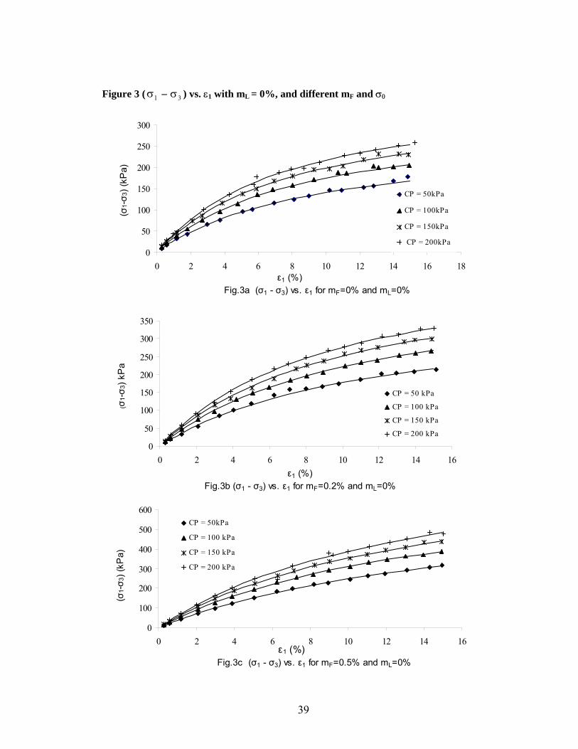
Figure 3 ( −1σ 3 ) vs. εσ 1 with mL = 0%, and different mF and σ0

Fig.3a (σ1 - σ3) vs. ε1 for mF=0% and mL=0%

0

50

100

150

200

250

300

0 2 4 6 8 10 12 14 16 18ε1 (%)

(σ1-σ 3

) (kP

a)

CP = 50kPa

CP = 100kPa

CP = 150kPa

CP = 200kPa

Fig.3b (σ1 - σ3) vs. ε1 for mF=0.2% and mL=0%

0

50

100

150

200

250

300

350

0 2 4 6 8 10 12 14 16ε1 (%)

(σ1-σ 3

) kP

a

CP = 50 kPa

CP = 100 kPa

CP = 150 kPa

CP = 200 kPa

Fig.3c (σ1 - σ3) vs. ε1 for mF=0.5% and mL=0%

0

100

200

300

400

500

600

0 2 4 6 8 10 12 14 1ε1 (%)

(σ1-σ 3

) (kP

a)

CP = 50kPa

CP = 100 kPa

CP = 150 kPa

CP = 200 kPa

6

39

Figure 4 ( −1σ 3 ) vs. εσ 1 with mF = 0.2%, mL = 5% and different σ0 and t

Fig.4.b (σ1 - σ3) vs. ε1 for mF=0.2%, mL=5% and t=14days

0

500

1000

1500

2000

0 2 4 6 8 10 12 14 16

ε1 (%)

(σ1-σ 3

) (kP

a)

CP = 50kPa

CP = 100 kPa

CP = 150 kPa

Fig.4.a (σ1 - σ3) vs. ε1 for mF=0.2%, mL=5% and t=7days

0

500

1000

1500

2000

0 2 4 6 8 10 12 14 16ε1 (%)

(σ1

- σ3)

(kP

a)CP = 50kPa

CP = 100 kPa

CP = 150 kPa

CP = 200 kPa

Fig.4.c (σ1 - σ3) vs. ε1 for mF=0.2%, mL=5% and t=28days

0

500

1000

1500

2000

2500

0 2 4 6 8 10 12 14 1ε1 (%)

(σ1-σ 3

) (kP

a)

CP = 50kPa

CP = 100 kPa

CP = 150 kPa

6

40

Figure 5 ( −1σ 3 ) vs 1 with mσ . ε F = 0.5%, mL = 5% and different σ0 and t

Fig.5.a (σ1 - σ3) vs. ε1 for mf=0.5%, ml=5% and t=7days

0

500

1000

1500

2000

2500

0 2 4 6 8 10 12 14 16ε1 (%)

(σ1-σ 3

) (kP

a)

CP = 50kPa

CP = 100 kPa

CP = 150 kPa

CP = 200 kPa

Fig.5.b (σ1 - σ3) vs. ε1 for mF=0.5%, mL=5% and t=14days

0

500

1000

1500

2000

2500

3000

0 2 4 6 8 10 12 14 16 1ε1 (%)

(σ1-σ 3

) (kP

a)

8

CP = 50kPaCP = 100 kPaCP = 150 kPaCP = 200 kPa

Fig5.c (σ1 - σ3) vs. ε1 for mF=0.5%, mL=5% and t=28days

0

500

1000

1500

2000

2500

3000

3500

4000

0 2 4 6 8 10 12 14 16ε1 (%)

(σ1-σ 3

) (kP

a)

CP = 50kPa

CP = 100 kPa

CP = 150 kPa

CP = 200 kPa

41

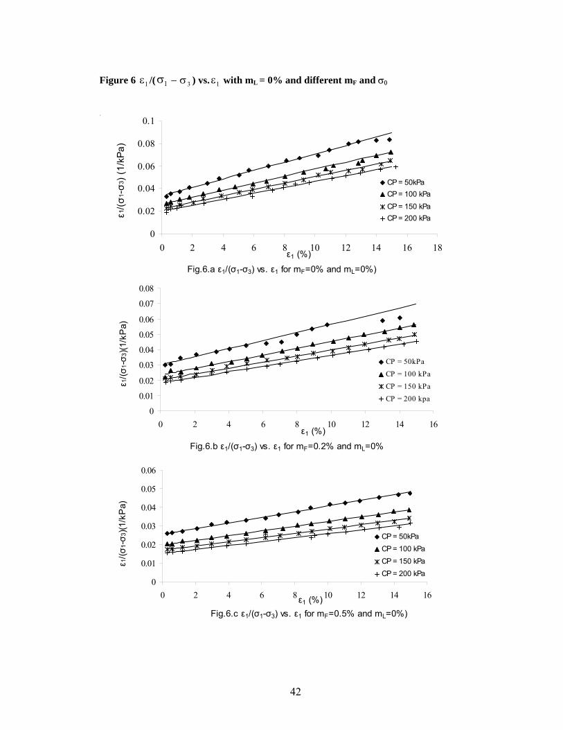
Figure 6 1 /( 1 − 3σ ) v 1ε with mε σ s . L = 0% and different mF and σ0

Fig.6.a ε1/(σ1-σ3) vs. ε1 for mF=0% and mL=0%)

0

0.02

0.04

0.06

0.08

0.1

0 2 4 6 8 10 12 14 16 18ε1 (%)

ε1/(σ

1 -σ3

) (1/

kPa)

CP = 50kPaCP = 100 kPaCP = 150 kPaCP = 200 kPa

ε

Fig.6.b ε1/(σ1-σ3) vs. ε1 for mF=0.2% and mL=0%

0

0.01

0.02

0.03

0.04

0.05

0.06

0.07

0.08

0 2 4 6 8 10 12 14 16ε1 (%)

ε 1/(σ

1-σ 3

)(1/k

Pa)

CP = 50kPaCP = 100 kPaCP = 150 kPaCP = 200 kpa

Fig.6.c ε1/(σ1-σ3) vs. ε1 for mF=0.5% and mL=0%)

0

0.01

0.02

0.03

0.04

0.05

0.06

0 2 4 6 8 10 12 14 16ε1 (%)

ε 1/(σ

1-σ 3

)(1/k

Pa)

CP = 50kPa CP = 100 kPaCP = 150 kPaCP = 200 kPa

42

Figure 7 1 /( 1 − 3σ ) v 1ε with mε σ s t . F = 0.2%, mL = 5% and different σ0 and

Fig.7.a ε1/(σ1-σ3) vs. ε1 for mF=0.2%, mL=5% and t=7days

0

0.002

0.004

0.006

0.008

0.01

0.012

0.014

0.016

0 2 4 6 8 10 12 14 16ε1 (%)

ε1/(σ

1 -σ3

)(1/

kPa)

CP = 50kPaCP = 100 kPaCP = 150 kPaCP = 200 kPa

Fig.7.b ε1/(σ1-σ3) vs. ε1 for mF=0.2%, mL=5% and t=14days

0

0.002

0.004

0.006

0.008

0.01

0.012

0.014

0 2 4 6 8 10 12 14 1ε1 (%)

ε 1/(σ

1-σ 3

)(1/

kPa)

6

CP = 50kPa

CP = 100 kPa

CP = 150 kPa

Fig.7.c ε1/(σ1-σ3) vs. ε1 for mF=0.2%, mL=5% and t=28days

0

0.002

0.004

0.006

0.008

0.01

0.012

0 2 4 6 8 10 12 14 1ε1 (%)

ε 1/(σ

1-σ 3

)(1/k

Pa)

CP = 50kPaCP = 100 kPa

CP = 150 kPa

6

43

Figure 8 1 /( 1 − 3σ ) v 1ε with mε σ s . F = 0.5%, mL = 5% and different σ0 and t

Fig.8.a ε1/(σ1-σ3) vs. ε1 for mF=0.5%, mL=5% and t=7days

0

0.002

0.004

0.006

0.008

0.01

0.012

0 2 4 6 8 10 12 14 1ε1 (%)

ε 1/(σ

1-σ 3

)(1/k

Pa)

6

CP = 50 kPaCP = 100 kPaCP = 150 kPaCP = 200 kPa

Fig.8.b ε1/(σ1-σ3) vs. ε1 for mF=0.5%, mL=5% and t=14days

0

0.002

0.004

0.006

0.008

0.01

0 5 10 15 20ε1 (%)

ε 1/(σ

1-σ 3

)(1/k

Pa)

CP = 50kPaCP = 100 kPaCP = 150 kPaCP = 200 kPa

Fig.8.c ε1/(σ1-σ3) vs. ε1 for mF=0.5%, mL=5% and t=28days

0

0.002

0.004

0.006

0.008

0 2 4 6 8 10 12 14 1ε1 (%)

ε 1/(σ

1-σ 3

)(1/k

Pa)

CP = 50 kPaCP = 100 kpaCP = 150 kPaCP = 200 kPa

6

44

Figure 9 ( 1 − 3 ) vs. 1ε with mσ σ 0 L = 0%, and different mF and σ

Fig.9.b (σ1-σ3) vs. ε1 for mL=0% and σ0=100kPa

050

100150200250300350400450

0 2 4 6 8 10 12 14 1ε1 (%)

(σ1-σ

3) (k

Pa)

6

mF=0%mF=0.2%mF=0.5%

Fig.9.c (σ1-σ3) vs. ε1 for mL=0% and σ0=150kPa

0

100

200

300

400

500

0 2 4 6 8 10 12 14 1ε1 (%)

(σ1-σ 3

) (kP

a)

mF=0%mF=0.2%mF=0.5%

Fig.9.a (σ1-σ3) vs. ε1 for mL=0% and σ0=50kPa

0

50

100

150

200

250

300

350

0 2 4 6 8 10 12 14 1ε1 (%)

(σ1-σ 3

) (kP

a)mF=0%mF=0.2%mF=0.5%

6

6

45

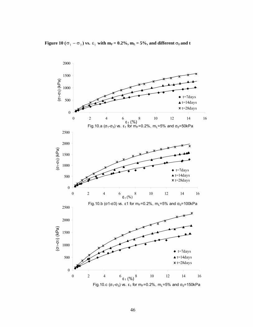
Figure 10 ( −1σ 3 ) vs. 1 with mσ ε F = 0.2%, mL = 5%, and different σ0 and t

Fig.10.a (σ1-σ3) vs. ε1 for mF=0.2%, mL=5% and σ0=50kPa

0

500

1000

1500

2000

0 2 4 6 8 10 12 14 16ε1 (%)

(σ1-σ 3

) (kP

a)

t=7dayst=14dayst=28days

Fig.10.b (σ1-σ3) vs. ε1 for mF=0.2%, mL=5% and σ0=100kPa

0

500

1000

1500

2000

2500

0 2 4 6 8 10 12 14 16ε1 (%)

(σ1-σ 3

) (kP

a)

t=7dayst=14dayst=28days

Fig.10.c (σ1-σ3) vs. ε1 for mF=0.2%, mL=5% and σ0=150kPa

0

500

1000

1500

2000

2500

0 2 4 6 8 10 12 14 16ε1 (%)

(σ1 -σ3

) (kP

a)

t=7dayst=14dayst=28days

46

Figure 11 ( 1 − 3 ) vs. 1ε with mσ σ F = 0.5%, mL = 5%, and different σ0 and t

Fig.11.a (σ1-σ3) vs. ε1 for mF=0.5%, mL=5% and σ0=50kPa

0

500

1000

1500

2000

2500

0 2 4 6 8 10 12 14 16ε1 (%)

(σ1-σ3

) (kP

a)

t=7dayst=14dayst=28days

Fig.11.c (σ1-σ3) vs. ε1 for mF=0.5%, mL=5% and σ0=150kPa

0500

100015002000250030003500

0 2 4 6 8 10 12 14 16 18ε1 (%)

(σ1-σ3

) (kP

a)

t=7dayst=14dayst=28days

Fig.11.d (σ1-σ3) vs. ε1 for mF=0.5%, mL=5% and σ0=200kPa

0

1000

2000

3000

4000

0 2 4 6 8 10 12 14 16ε1 (%)

(σ1-σ

3) (

kPa)

t=7dayst=14dayst=28days

Fig.11.b (σ1-σ3) vs. ε1 for mF=0.5%, mL=5% and σ0=100kPa

0

500

1000

1500

2000

2500

3000

0 2 4 6 8 10 12 14 16ε1 (%)

(σ1-σ3

) (kP

a)

t=7dayst=14dayst=28days

47

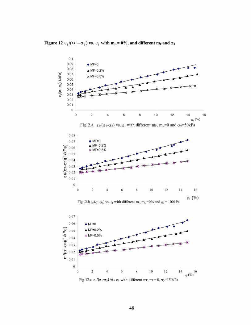
Figure 12 /( 1 3 ) vs. 1ε with m1ε σ − σ L = 0%, and different mF and σ0

Fig12.a. ε1/(σ1-σ3) vs. ε1 with different mF, mL=0 and σ0=50kPa

00.010.020.030.040.050.060.070.080.090.1

0 2 4 6 8 10 12 14 16ε1 (%)

ε 1/(σ

1-σ 3

)(1/

kPa)

MF=0

MF=0.2%

MF=0.5%

Fig.12.c ε1/(σ1-σ3) vs. ε1 with different mF, mL= 0, σ0=150kPa

0

0.01

0.02

0.03

0.04

0.05

0.06

0.07

0 2 4 6 8 10 12 14 16ε1 (%)

ε1/(σ

1 -σ3

)(1/

kPa)

MF=0

MF=0.2%MF=0.5%

Fig.12.b ε1/(σ1-σ3) vs. ε1 with different mF, mL =0% and σ0 = 100kPa

0

0.01

0.02

0.03

0.04

0.05

0.06

0.07

0.08

0 2 4 6 8 10 12 14 16

ε1 (%)

ε1/(σ

1 -σ3

)(1/

kPa)

MF=0MF=0.2%MF=0.5%

48

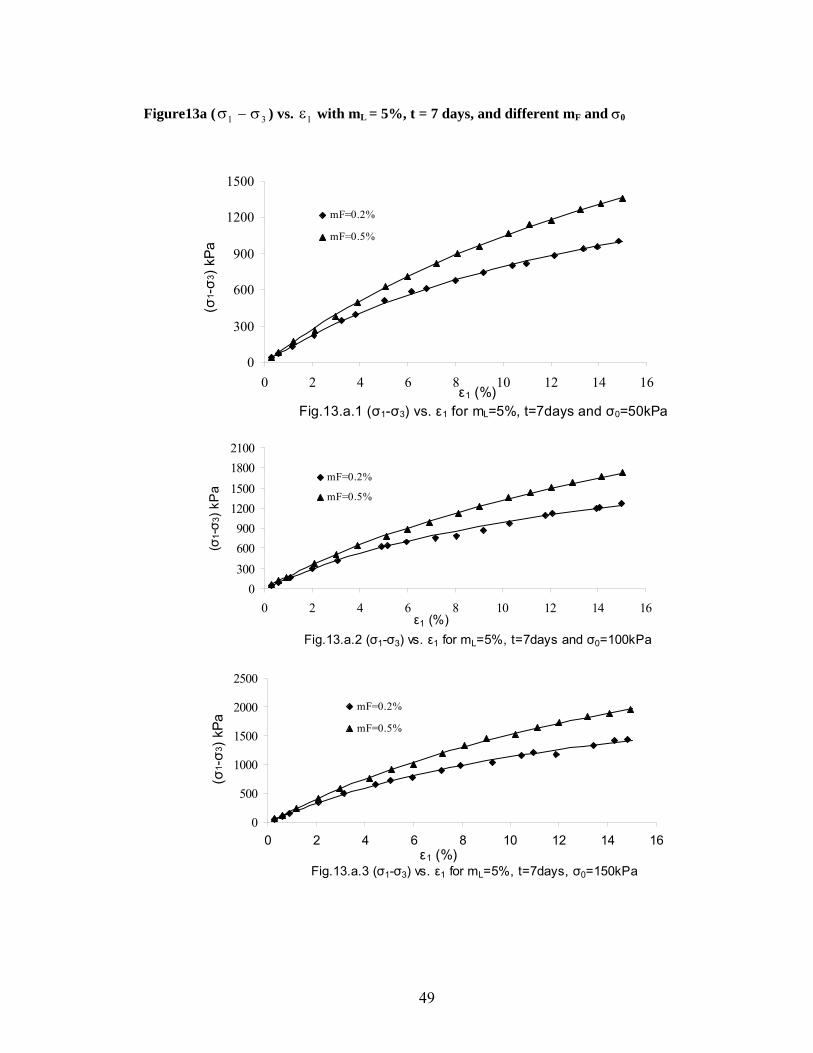
Figure13a ( −1σ 3 ) vs. 1 with mσ ε L = 5%, t = 7 days, and different mF and σ0

Fig.13.a.3 (σ1-σ3) vs. ε1 for mL=5%, t=7days, σ0=150kPa

0

500

1000

1500

2000

2500

0 2 4 6 8 10 12 14 16ε1 (%)

(σ1 -σ3

) kPa

mF=0.2%

mF=0.5%

Fig.13.a.2 (σ1-σ3) vs. ε1 for mL=5%, t=7days and σ0=100kPa

0300600900

1200150018002100

0 2 4 6 8 10 12 14 16ε1 (%)

(σ1-σ 3

) kP

a

mF=0.2%

mF=0.5%

Fig.13.a.1 (σ1-σ3) vs. ε1 for mL=5%, t=7days and σ0=50kPa

0

300

600

900

1200

1500

0 2 4 6 8 10 12 14 16ε1 (%)

(σ1 -σ3

) kPa

mF=0.2%

mF=0.5%

49

Figure13b ( 1 − 3 ) vs. 1ε with mσ σ 0 L = 5%, t = 14 days, and different mF and σ

Fig.13.b.1 (σ1-σ3) vs. ε1 for mL=5%, t=7days and σ0=50kPa

0

500

1000

1500

2000

0 2 4 6 8 10 12 14 1ε1 (%)

(σ1 -σ3

) kP

a

6

mF=0.2%

mF=0.5%

Fig.13.b.3 (σ1-σ3) vs. ε1 for mL=5%, t=14days and σ0=150kPa

0

500

1000

1500

2000

2500

3000

0 5 10 15 20ε1 (%)

(σ1 -σ3

) kPa

mF=0.2%

mF=0.5%

Fig.13.b.2 (σ1-σ3) vs. ε1 for mL=5%, t=14days and σ0=100kPa

0

500

1000

1500

2000

2500

0 2 4 6 8 10 12 14 1ε1 (%)

(σ1-σ 3

) kP

a

mF=0.2%

mF=0.5%

6

50

Figure13c ( −1σ 3 ) vs. 1 with mσ ε L = 5%, t = 28 days, and different mF and σ0

Fig.13.c.1 (σ1-σ3) vs. ε1 for mL=5%, t=28days and σ0=50kPa

0

500

1000

1500

2000

2500

0 2 4 6 8 10 12 14 1ε1 (%)

(σ1-σ 3

) (k

Pa)

mF=0.2%

mF=0.5%

6

Fig.13.c.2 (σ1-σ3) vs. ε1 for mL=5%, t=28days and σ0=100kPa

0

500

1000

1500

2000

2500

3000

0 2 4 6 8 10 12 14 1 ε1 (%)

(σ1-σ 3

) (kP

a)

mF=0.2%

mF=0.5%

6

51

Figure14a 1 /( 1 − 3σ ) vs 1ε with mε σ . 0 L = 5%, t = 7 days, and different mF and σ

Fig.14.a3 ε1/(σ1-σ3) vs. ε1 for mL=5%, t=7days and σ0=150kPa

0

0.002

0.004

0.006

0.008

0.01

0.012

0 2 4 6 8 10 12 14 16ε1 (%)

ε 1/(σ

1-σ 3

) (1/

kPa)

mF=0.2%mF=0.5%

Fig.14.a2 ε1/(σ1-σ3) vs. ε1 for mL=5%, t=7days and σ0=100kPa

0

0.002

0.004

0.006

0.008

0.01

0.012

0.014

0 2 4 6 8 10 12 14 16ε1 (%)

ε 1/(σ

1-σ 3

) (1/

kPa)

mF=0.2%mF=0.5%

Fig.14a.1 ε1/(σ1-σ3) vs. ε1 for mL=5%, t=7days and σ0=50kPa

0

0.004

0.008

0.012

0.016

0 2 4 6 8 10 12 14 16 ε1 (%)

ε 1/(σ

1-σ 3

)(1/k

Pa)

mF=0.2%

mF=0.5%

52

Figure14b 1 /( 1 − 3 ) vs 1ε with mε σ σ . 0 L = 5%, t = 14 days, and different mF and σ

Fig.14.b2 ε1/(σ1-σ3) vs. ε1 for mL=5%, t=14days and σ0=100kPa

0

0.002

0.004

0.006

0.008

0.01

0.012

0 2 4 6 8 10 12 14 1ε1 (%)

ε 1/(σ

1-σ 3

) (1/

kPa)

mF=0.2%

mF=0.5%

Fig14.b1 ε1/(σ1-σ3) vs. ε1 for mL=5%, t=14days and σ0=50kPa

0

0.002

0.004

0.006

0.008

0.01

0.012

0.014

0 2 4 6 8 10 12 14 1ε1 (%)

ε 1/(σ

1-σ 3

) (1/

kPa)

mF=0.2%mF=0.5%

6

6

Fig.14.b3 ε1/(σ1-σ3) vs. ε1 with mL= 5%, t=14d, σ0=150kPa

0

0.001

0.002

0.003

0.004

0.005

0.006

0.007

0.008

0.009

0 2 4 6 8 10 12 14 16ε1 (%)

ε 1/(σ

1-σ 3

) (1/

kPa)

MF=0.2%

MF=0.5%

18

53

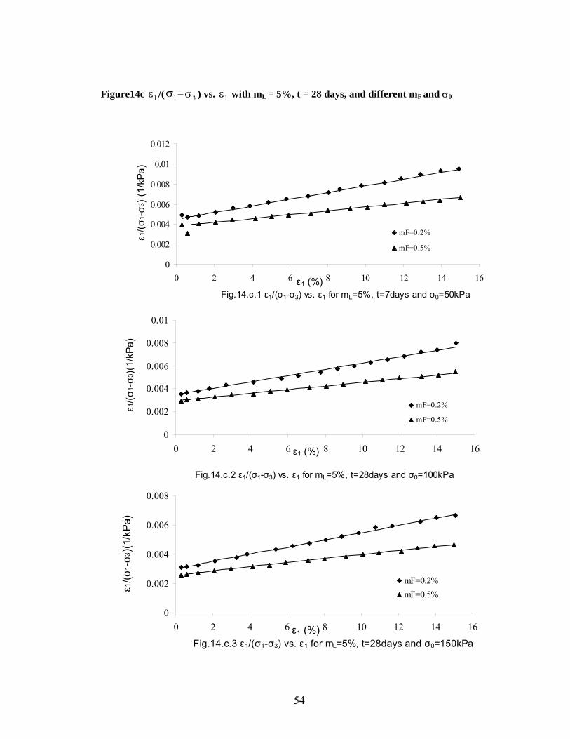
Figure14c 1 /( 1 − 3σ ) vs 1ε with mε σ . 0 L = 5%, t = 28 days, and different mF and σ

Fig.14.c.3 ε1/(σ1-σ3) vs. ε1 for mL=5%, t=28days and σ0=150kPa

0

0.002

0.004

0.006

0.008

0 2 4 6 8 10 12 14 16ε1 (%)

ε1/(σ

1 -σ3

)(1/

kPa)

mF=0.2%mF=0.5%

Fig.14.c.2 ε1/(σ1-σ3) vs. ε1 for mL=5%, t=28days and σ0=100kPa

0

0.002

0.004

0.006

0.008

0.01

0 2 4 6 8 10 12 14 16ε1 (%)

ε1/(σ

1 -σ3

)(1/

kPa)

mF=0.2%

mF=0.5%

Fig.14.c.1 ε1/(σ1-σ3) vs. ε1 for mL=5%, t=7days and σ0=50kPa

0

0.002

0.004

0.006

0.008

0.01

0.012

0 2 4 6 8 10 12 14ε1 (%)

ε1/(σ

1 -σ3

) (1/

kPa)

mF=0.2%

mF=0.5%

16

54

Figure 15 Mohr’s circles with mL = 0% and different mF

Fig.15c τ vs. σ for mL=0% and mF=0.5%

0

50

100

150

200

250

300

0 100 200 300 400 500 600 700 800σ (kPa)

τ (k

Pa)

Fig.15b τ vs. σ for mL=0% and mF=0.2%

0

50

100

150

200

250

0 100 200 300 400 500 600σ (kPa)

τ (k

Pa)

Fig. 15a τ vs. σ for mF=0% and mL=0%

0

40

80

120

160

200

0 100 200 300 400 500σ (kPa)

τ (k

Pa)

55

Figure 16 Mohr’s circles with mL = 5% and mF= 0.2% and different t

Fig. 16c τ vs. σ for mL=5%, mF=0.2% and t=28days

0

200

400

600

800

1000

1200

1400

1600

1800

0 500 1000 1500 2000 2500 3000σ (kPa)

τ (k

Pa)

Fig. 16b τ vs. σ for mL=5%, mF=0.2% and t=14days

0

400

800

1200

1600

2000

0 500 1000 1500 2000 2500

σ (kPa)

τ (kP

a)

Fig. 16a τ vs. σ for mL=5%, mF=0.2%, and t=7days

0

200

400

600

800

1000

1200

0 500 1000 1500 2000σ (kPa)

τ (kP

a)

56

Figure 17 Mohr’s circles with mL = 5%, mF = 0.5% and different t

Fig. 16b τ vs. σ for mL=5%, mF=0.2% and t=14days

0

400

800

1200

1600

2000

0 500 1000 1500 2000 2500σ (kPa)

τ (k

Pa)

Fig. 16c τ vs. σ for mL=5%, mF=0.2% and t=28days

0

200

400

600

800

1000

1200

1400

1600

1800

0 500 1000 1500 2000 2500 3000σ (kPa)

τ (kP

a)

Fig. 16a τ vs. σ for mL=5%, mF=0.2%, and t=7days

0

200

400

600

800

1000

1200

0 500 1000 1500 2000σ (kPa)

τ (kP

a)

57

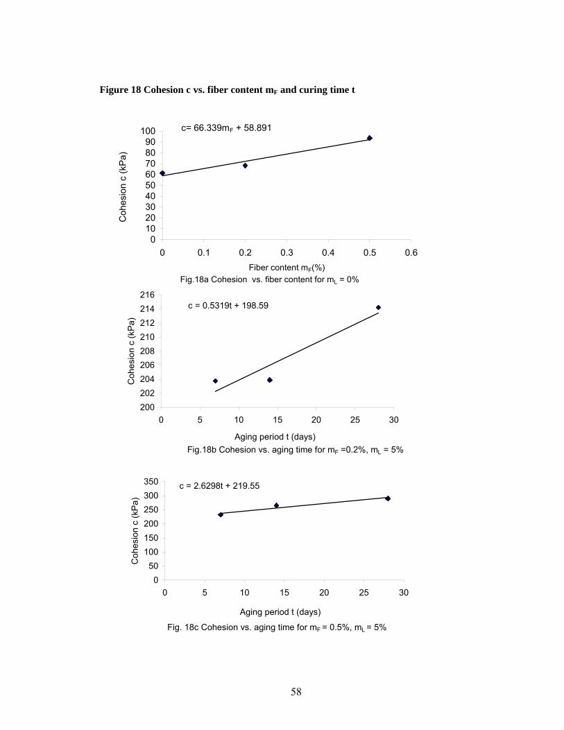
Figure 18 Cohesion c vs. fiber content mF and curing time t

Fig.18a Cohesion vs. fiber content for mL = 0%

c= 66.339mF + 58.891

0102030405060708090

100

0 0.1 0.2 0.3 0.4 0.5 0.6Fiber content mF(%)

Coh

esio

n c

(kP

a)

Fig.18b Cohesion vs. aging time for mF =0.2%, mL = 5%

c = 0.5319t + 198.59

200202204206208210212214216

0 5 10 15 20 25 30

Aging period t (days)

Coh

esio

n c

(kP

a)

Fig. 18c Cohesion vs. aging time for mF = 0.5%, mL = 5%

c = 2.6298t + 219.55

050

100150200250300350

0 5 10 15 20 25 30

Aging period t (days)

Coh

esio

n c

(kP

a)

58

Figure 19 Friction angle φ vs. fiber content mF and curing time t

Fig. 19a Friction angle vs. fiber content for mL = 0%

Ф = 16.658mF + 12.313

0

5

10

15

20

25

0 0.1 0.2 0.3 0.4 0.5 0.6

Fiber content mF (%)

Fric

tion

angl

e Ф

(0 )

Fig. 19b Friction angle vs. aging time for mF= 0.2%, mL = 5%

Ф = 0.501t + 37.45

0102030405060

0 5 10 15 20 25 30

Aging period t (days)

Fric

tion

angl

e Ф

(0 )

Fig. 19c Friction angle vs. aging time for mF= 0.5%, mL= 5%

Ф = 0.4t + 43.7

44

46

48

50

52

54

56

0 5 10 15 20 25 30

Aging period t (days)

Fric

tion

angl

e Ф

(0 )

59

Figure 20 σd ~εd with mL=2%, mF= 0.2%, t =7 days, and different σ0 and N

020406080

100120140160180

0 0.05 0.1 0.15 0.2 0.25 0.3εd (%)

b. N=500, t =7days, mL=2% and mF=0.2%

σ d (k

Pa)

CP=50KPa

CP=100KPa

CP=150KPa

020406080

100120140160180

0 0.05 0.1 0.15 0.2 0.25εd (%)

b. N=100, t =7days, mL=2% and mF=0.2%

σ d (k

Pa)

CP=50KPa

CP=100KPa

CP=150KPa

0

50

100

150

200

0 0.05 0.1 0.15 0.2 0.25 0.3εd (%)

a. N=50, t =7days, mL=2% and mF=0.2%

σ d (k

Pa) CP=50KPa

CP=100KPa

CP=150KPa

CP=21kPa

60

Figure 21 σd ~εd with mL=5%, mF= 0.2%, t =7 days, and different σ0 and N

020406080

100120140160180

0 0.05 0.1 0.15 0.2 0.25 0.3εd (%) c. N=500, t =7days, mL=5% and mF=0.2%

σd (k

Pa)

CP=50KPa

CP=100KPa

CP=150KPa

0

50

100

150

200

0 0.05 0.1 0.15 0.2 0.25 0.3εd (%) b. N=100, t =7days, mL=5% and mF=0.2%

σ d (k

Pa)

CP=50KPa

CP=100KPa

CP=150KPa

0

20

40

60

80

100

120

140

0 0.05 0.1 0.15 0.2 0.25εd (%) a. N=50, t =7days, mL=5% and mF =0.2%

σd (k

Pa) CP=50KPa

CP=100KPa

CP=150KPa

CP=21kPa

61

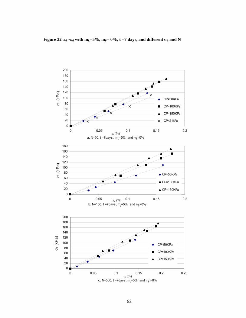
Figure 22 σd ~εd with mL=5%, mF= 0%, t =7 days, and different σ0 and N

020406080

100120140160180200

0 0.05 0.1 0.15 0.2 0.25εd (%)

c. N=500, t =7days, mL=5% and mF =0%

σ d (k

Pa)

CP=50KPa

CP=100KPa

CP=150KPa

020406080

100120140160180

0 0.05 0.1 0.15 0.2εd (%) b. N=100, t =7days, mL=5% and mF=0%

σ d (k

Pa)

CP=50KPa

CP=100KPa

CP=150KPa

0

2040

6080

100

120140

160180

200

0 0.05 0.1 0.15 0.2εd (%)

a. N=50, t =7days, mL=5% and mF=0%

σ d (k

Pa)

CP=50KPa

CP=100KPa

CP=150KPa

CP=21kPa

62

Figure 23 σd ~εd with mL=2%, mF= 0.5%, t =7 days, and different σ0 and N

0

20

40

60

80

100

120

140

160

0 0.05 0.1 0.15 0.2 0.25 0.3 0.35εd (%)

c. N=500, t =7days, mL=2% and mF=0.5%

σ d (k

Pa)

CP=50KPa

CP=100KPa

CP=150KPa

0

20

40

60

80

100

120

140

160

0 0.05 0.1 0.15 0.2 0.25 0.3 0.35

εd (%) b. N=100, t =7days, mL=2% and mF=0.5%

σ d (k

Pa)

CP=50KPa

CP=100KPa

CP=150KPa

Li

0

2040

60

80

100120

140

160

0 0.05 0.1 0.15 0.2 0.25 0.3 0.35εd (%)

a. N=50, t 7days, mL=2% and mF =0.5%

σ d (k

Pa) CP=50KPa

CP=100KPa

CP=150KPa

63

Figure 24 σd ~εd with mL=2%, mF= 0.2%, t=7 days, and different σ0 and N

0

20

40

60

80

100

120

140

0 0.05 0.1 0.15 0.2εd (%)

a. N=50, t =7days, mL=5% and mF=0.2%

σ d (k

Pa)

CP=50KPa

CP=100KPaCP=150KPa

020406080

100120140160180200

0 0.05 0.1 0.15 0.2 0.25 0.3εd (%) b. N=100, t =7days, mL=5% and mF=0.2%

σ d (k

Pa)

CP=50KPa

CP=100KPa

CP=150KPa

Li

020406080

100120140160180

0 0.05 0.1 0.15 0.2 0.25 0.3εd (%)

c. N=500, t =7 days, mL =5% and mF = 0.2%

σ d (k

Pa)

CP=50KPa

CP=100KPa

CP=150KPa

Li

64

Figure 25 σd ~εd with mL=5%, mF= 0.5%, t =7 days, and different σ0 and N

020406080

100120140160180

0 0.05 0.1 0.15 0.2 0.25 0.3 0.35εd (%)

c. N = 500, t = 7 days, mL= 5% and mF = 0.5%

σ d (k

Pa)

CP=50KPaCP=100KPaCP=150KPa

0

50

100

150

200

0 0.05 0.1 0.15 0.2 0.25 0.3εd (%)

a. N = 50, t =7 days, mL= 5% and mF = 0.5%

σ d (k

Pa)

CP=50KPaCP=100KPaCP=150KPa

020406080

100120140160180

0 0.05 0.1 0.15 0.2 0.25 0.3εd (%)

b. N = 100, t = 7 days, mL = 5% and mF = 0.5%

σ d (k

Pa)

CP=50KPaCP=100KPaCP=150KPa

65

Figure 26 σd ~εd with mL=2%, mF= 0%, t =14 days, and different σ0 and N

020406080

100120140160180200

0 0.05 0.1 0.15 0.2εd (%)

a. N = 50, t =14, mL= 2% and mF = 0%

σ d (k

Pa)

CP= 21 kPaCP = 50 kPaCP = 100 kPaCP = 150 kPa

020406080

100120140160180200

0 0.05 0.1 0.15 0.2 0.25

εd (%) b. N = 100, t = 14 days, mL = 2 % and mF = 0 %

σ d (k

Pa)

CP = 50 kPa

CP = 100 kPa

CP = 150 kPa

020406080

100120140160180200

0 0.05 0.1 0.15 0.2 0.25εd (%)

c. N = 500, t = 14 days, mL= 2 % and mF = 0 %

σ d (k

Pa) CP = 50 kPa

CP = 100 kPa

CP = 150 kPa

66

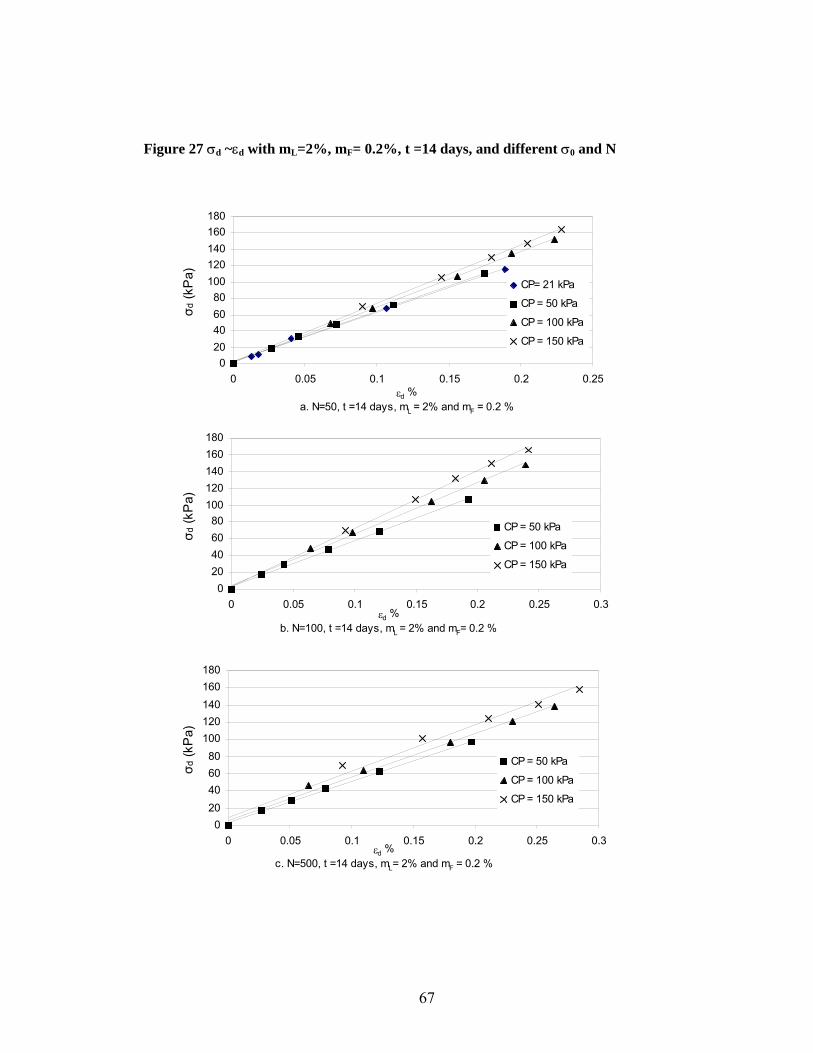
Figure 27 σd ~εd with mL=2%, mF= 0.2%, t =14 days, and different σ0 and N

020406080

100120140160180

0 0.05 0.1 0.15 0.2 0.25εd %

a. N=50, t =14 days, mL = 2% and mF = 0.2 %

σ d (k

Pa)

CP= 21 kPa

CP = 50 kPa

CP = 100 kPa

CP = 150 kPa

020406080

100120140160180

0 0.05 0.1 0.15 0.2 0.25 0.3εd %

b. N=100, t =14 days, mL = 2% and mF= 0.2 %

σ d (k

Pa)

CP = 50 kPa

CP = 100 kPa

CP = 150 kPa

020406080

100120140160180

0 0.05 0.1 0.15 0.2 0.25 0.3εd %

c. N=500, t =14 days, mL= 2% and mF = 0.2 %

σ d (k

Pa)

CP = 50 kPa

CP = 100 kPa

CP = 150 kPa

67

Figure 28 σd ~εd with mL=5%, mF= 0.2%, t =14 days, and different σ0 and N

020406080

100120140160180200

0 0.05 0.1 0.15 0.2εd %a. N=50, t =14 days, mL = 5 % and mF = 0.2 %

σ d (k

Pa)

CP= 21 kPa

CP = 50 kPa

CP = 100 kPa

CP = 150 kPa

020406080

100120140160180

0 0.05 0.1 0.15 0.2 0.25εd %

c. N=500, t =14 days, mL = 5 % and mF = 0.2 %

σ d (k

Pa)

CP = 50 kPa

CP = 100 kPa

CP = 150 kPa

020406080

100120140160180200

0 0.05 0.1 0.15 0.2 0.25εd %

b. N=100, t =14 days, mL = 5 % and mF= 0.2 %

σ d (k

Pa)

CP = 50 kPa

CP = 100 kPa

CP = 150 kPa

68

Figure 29 σd ~εd with mL=2%, mF= 0.5%, t =14 days, and different σ0 and N

020406080

100120140160180

0 0.05 0.1 0.15 0.2 0.25 0.3 0.35εd %

a. N=50, t =14 days, mL = 2 % and mF= 0.5 %

σ d (k

Pa)

CP= 21 kPa

CP = 50 kPa

CP = 100 kPa

CP = 150 kPa

020406080

100120140160

0 0.05 0.1 0.15 0.2 0.25 0.3 0.35 0.4

εd % b. N=100, t =14 days, mL = 2 % and mF= 0.5 %

σ d (k

Pa)

CP = 50 kPa

CP = 100 kPa

CP = 150 kPa

020406080

100120140160

0 0.05 0.1 0.15 0.2 0.25 0.3 0.35 0.4

εd % c. N=500, t =14 days, mL = 2 % and mF = 0.5 %

σ d (k

Pa)

CP = 50 kPa

CP = 100 kPa

CP = 150 kPa

69

Figure 30 σd ~εd with mL=5%, mF= 0.5%, t =14 days, and different σ0 and N

020406080

100120140160180200

0 0.05 0.1 0.15 0.2 0.25εd %

a. N=50, t =14 days, mL = 5 % and mF = 0.5 %

σ d (k

Pa)

CP= 21 kPa

CP = 50 kPa

CP = 100 kPa

CP = 150 kPa

020406080

100120140160180

0 0.05 0.1 0.15 0.2 0.25 0.3εd %

c. N=500, t =14 days, mL = 5 % and mF= 0.5 %

σ d (k

Pa)

CP = 50 kPa

CP = 100 kPa

CP = 150 kPa

020406080

100120140160180200

0 0.05 0.1 0.15 0.2 0.25 0.3εd %

b. N=100, t =14 days, mL= 5 % and mF = 0.5 %

σ d (k

Pa)

CP = 50 kPa

CP = 100 kPa

CP = 150 kPa

70

Figure 31 σd ~εd with mL=2%, mF= 0%, t =28 days, and different σ0 and N

020406080

100120140160180200

0 0.02 0.04 0.06 0.08 0.1 0.12 0.14 0.16εd (%)

a. N=50, t =28days, mL=2% and mF =0%

σ d (k

Pa)

CP=50KPa

CP=100KPa

CP=150KPa

CP=21kPa

020406080

100120140160180200

0 0.02 0.04 0.06 0.08 0.1 0.12 0.14 0.16εd (%)

b. N=100, t =28days, mL=2% and mF=0%

σ d (k

Pa)

CP=50KPaCP=100KPaCP=150KPa

020406080

100120140160180200

0 0.05 0.1 0.15 0.2εd (%)

c. N=150, t =28 days, mL=2% and mF=0%

σ dη(k

Pa)

CP=50KPa

CP=100KPa

CP=150KPa

71

Figure 32 σd ~εd with mL=2%, mF= 0.2%, t =28 days, and different σ0 and N

0

20

40

60

80

100

120

140

160

0 0.05 0.1 0.15 0.2 0.25 0.3 0.35εd (%)

c. N=500, t =28days, mL=2% and mF =0.2%

σd (k

Pa)

CP=50KPa

CP=100KPa

CP=150KPa

020406080

100120140160180

0 0.05 0.1 0.15 0.2 0.25 0.3εd (%)

b. N=100, t =28days, mL=2% and mF=0.2%

σd (k

Pa)

CP=50KPa

CP=100KPa

CP=150KPa

020406080

100120140160180200

0 0.05 0.1 0.15 0.2 0.25 0.3εd (%)

a. N=50, t =28days, ml=2% and mf =0.2%

σd (k

Pa)

CP=50KPa

CP=100KPa

CP=150KPa

CP=21kPa

72

Figure 33 σd ~εd with mL=5%, mF= 0.2%, t =28 days, and different σ0 and N

020406080

100120140160180200

0 0.05 0.1 0.15 0.2 0.25εd (%)

c. N=500, t =28days, mL=5% and mF =0.2%

σ d (k

Pa)

CP=50KPa

CP=100KPa

CP=150KPa

020406080

100120140160180200

0 0.05 0.1 0.15 0.2 0.25εd (%)

b. N=100, t =28days, mL=5% and mF =0.2%

σ d (k

Pa)

CP=50KPa

CP=100KPa

CP=150KPa

020406080

100120140160180200

0 0.05 0.1 0.15 0.2 0.25εd (%) a. N=50, t =28days, mL=5% and mF =0.2%

σ d (k

Pa) CP=50KPa

CP=100KPa

CP=150KPa

CP=21kPa

73

Figure 34 σd ~εd with mL=0%, mF= 0.2%, t =28 days, and different σ0 and N

020406080

100120140160180200

0 0.05 0.1 0.15 0.2εd (%) N=500, t =28days, mL=5% and mF =0%

σ d (k

Pa)

CP=50KPa

CP=100KPa

CP=150KPa

020406080

100120140160180200

0 0.05 0.1 0.15 0.2εd (%) b. N=100, t =28days, mL=5% and mF =0%

σ d (k

Pa)

CP=50KPa

CP=100KPa

CP=150KPa

020406080

100120140160180200

0 0.05 0.1 0.15 0.2εd (%) a. N=50, t =28days, mL=5% and mF=0%

σd (k

Pa)

CP=50KPa

CP=100KPa

CP=150KPa

CP=21kPa

74

Figure 35 σd ~εd with mL=2%, mF= 0.5%, t =28 days, and different σ0 and N

010

2030

4050

6070

8090

100

0 0.05 0.1 0.15 0.2 0.25 0.3εd (%)

c. N=500, t =28days, mL=2% and mF =0.5%

σd (k

Pa)

CP=50KPa

CP=100KPa

CP=150KPa

0

20

40

60

80

100

120

140

0 0.05 0.1 0.15 0.2 0.25 0.3εd (%)

b. N=100, t =28days, mL=2% and mF =0.5%

σ d (k

Pa)

CP=50KPa

CP=100KPa

CP=150KPa

0

20

40

60

80

100

120

140

160

0 0.05 0.1 0.15 0.2 0.25 0.3 0.35 0.4εd (%)

a. N=50, t =28days, mL=2% and mF=0.5%

σ d (k

Pa) CP=50KPa

CP=100KPa

CP=150KPa

CP=21kPa

75

Figure 36 σd ~εd with mL=5%, mF= 0.5%, t =28 days, and different σ0 and N

020406080

100120140160180

0 0.05 0.1 0.15 0.2 0.25εd (%) c. N= 500, t =28 days, mL= 5% and mF = 0.5%

σ d (k

Pa)

CP=50KPa

CP=100KPa

CP=150KPa

0

50

100

150

200

250

0 0.05 0.1 0.15 0.2 0.25εd (%)

a. N = 50, t = 28 days, mL = 5% and mF = 0.5%

σ d (k

Pa)

CP=50KPa

CP=100KPa

CP=150KPa

CP=21kPa

020406080

100120140160180200

0 0.05 0.1 0.15 0.2 0.25εd (%)

b. N = 100, t = 28 days, mL= 5% and mF = 0.5%

σd (k

Pa)

CP=50KPa

CP=100KPa

CP=150KPa

Li

76

Figure 37 G vs. N, mL, mF, t and σ0

G = 49019t0.0537

020000400006000080000

100000120000

0 5 10 15 20 25 30t (days)e. G vs. t w ith different mL, mF, N and σ0

G (k

Pa)

G = 34990σ00.1097

020000400006000080000

100000120000

0 20 40 60 80 100 120 140 160σ0 (kPa)

a G vs. σ0 w ith different mL, mF, t and N

G (k

Pa)

G = 56892mF0.0099

020000400006000080000

100000120000

0 0.1 0.2 0.3 0.4 0.5 0.6mF (%)b. G vs. mF w ith dif ferent mF, t, N and σ0

G (k

Pa)

G = 55943mL0.0122

020000400006000080000

100000120000

0 1 2 3 4 5 6mL (%)

c G vs. mL w ith different mF, t, N and σ0

G (k

Pa)

G = 77623N-0.0661

020000400006000080000

100000120000

0 100 200 300 400 500 600Νd. G vs. Ν w ith different mL, mF, t and σ0

G (k

Pa)

77

010000

20000300004000050000

6000070000

0 100 200 300 400 500 600 700σm (kPa)

a. t= 7 days, mF=0.5%, mL=5%

Mr (

KPa)

N = 50N = 100N = 500

0

20000

40000

60000

80000

100000

0 100 200 300 400 500 600 700σm (kPa)

d. t= 7 days, mF=0.2%, mL=2%

Mr (

KPa)

N = 50N = 100N = 500

010000200003000040000500006000070000

0 100 200 300 400 500 600 700σm (kPa)

b. t= 7 days, mF=0.5%, mL=2%

Mr (

KPa)

N =50N = 100

N = 500

0

20000

40000

60000

80000

100000

0 100 200 300 400 500 600 700σm (kPa)

c. t= 7 days, mF=0.2%, mL=5%

Mr (

KPa)

N = 50

N = 100

N = 500

Figure 38 Mr ~σm with t =7 days and different mF, mL and N

78

0

20000

40000

60000

80000

100000

0 50 100 150 200 250σm (kPa)a. t=14 days, mF=0.5% and mL =5%

Mr (

kPa)

N = 50N = 100N = 500

010000200003000040000500006000070000

0 50 100 150 200 250σm (kPa)

b. t =14 days, mF= 0.5% and mL =2%

Mr (

kPa)

N = 50

N = 100N = 500

0

20000

40000

60000

80000

100000

120000

0 50 100 150 200 250σm (kPa)

c. t =14 days, mF = 0.2% and mL= 5%

Mr (

kPa)

N = 50N = 100N = 500

0100002000030000400005000060000700008000090000

0 50 100 150 200 250σm (kPa)

d. t =14 days, mF = 0.2% and mL =2%

Mr (

kPa)

N = 50N = 100N = 500

Figure 39 Mr ~σm with t =14 days and different mF, mL and N

79

0

20000

40000

60000

80000

100000

120000

0 100 200 300 400 500 600 700σm (kPa)

t= 28 days, mF=0.5%, mL=5%

Mr (

KPa)

N =50N = 100

N =5000

20000

40000

60000

80000

100000

120000

0 100 200 300 400 500 600 700σm (kPa)

a. t= 28 days, mF=0.5%, mL=5%

Mr (

KPa)

N =50N = 100

N =500

0

20000

40000

60000

80000

100000

0 100 200 300 400 500 600 700

σm (kPa)d. t= 28 days, mF=0.2%, mL=2%

Mr (

KPa)

N = 50N =100N = 500

0

20000

40000

60000

80000

100000

120000

0 100 200 300 400 500 600 700

σm (kPa)c. t= 28 days, mF=0.2%, mL=5%

Mr (

KPa)

N = 50N =100N = 500

0

10000

20000

30000

40000

50000

60000

0 100 200 300 400 500 600 700

σm (kPa) b. t= 28 days, mF=0.5%, mL=2%

Mr (

KPa)

N = 50N =100N = 500

Figure 40 Mr ~σm with t =28 days and different mF, mL and N

80

THE LIST OF TABLES Table 1 Specimens for static tests with fiber and without lime

Fiber Content

mF Lime Content

mL Cell Pressure

σ0 Group

Number Specimen Number

( %) (%) (kPa) S11 0 0 50 S12 0 0 100 S13 0 0 150

1

S14 0 0 200 F5 0.2 0 50 F6 0.2 0 100 F7 0.2 0 150

2

F8 0.2 0 200 F5-5 0.5 0 50 F5-6 0.5 0 100 F5-7 0.5 0 150

3

F5-8 0.5 0 200

81

Table 2 Specimens for static tests with fiber and lime

Fiber Content

mF

Lime Content mL

Cell Pressure σ0

Aging Periods

Group Number

Specimen Number

( %) (%) (kPa) (day) Slf2 0.2 5 0 7

Slf1, 11, 9 0.2 5 50 7 Slf6, 17 0.2 5 100 7

4

Slf3, 15 0.2 5 150 7 Slf5, 12, 16 0.2 5 50 14

Slf4 0.2 5 100 14

5

Slf7, 8 0.2 5 150 14 Slf14 0.2 5 50 28 Slf13 0.2 5 100 28

6

Slf18, 19, 20 0.2 5 150 28 Slf5-9 0.5 5 0 7 Slf5-1 0.5 5 50 7 Slf5-2 0.5 5 100 7

Slf5-4, 5-10 0.5 5 150 7

7

Slf5-6, 5-12 0.5 5 200 7 Slf5-3 0.5 5 50 14 Slf5-5 0.5 5 100 14

Slf5-7, 5-11 0.5 5 150 14

8

Slf5-8 0.5 5 200 14 Slf5-16 0.5 5 50 28 Slf5-13 0.5 5 100 28 Slf5-14 0.5 5 150 28

9

Slf5-15 0.5 5 200 28

82

Table 3 Specimens for dynamic tests with mF = 0% and mL = 2%

Fiber Content

mF

Lime Content

mL

Cell Pressureσ0

Aging Time

t

Repetition Number

N

Dry Unit Weight

γd Group Number

Specimen Number

(%) (%) (kPa) (day) (g/cm3) 21002050 21 A0002050 50 B0002050 100 1

C0002050 150

50

A0002100 50 B0002100 100 2 C0002100 150

100

A0002500 50 B0002500 100 3 C0002500

0 2

150

7

500

1.88

21142050 21 A1402050 50 B1402050 100 4

C1402050 150

50

A1402100 50 B1402100 100 5 C1402100 150

100

A1402500 50 B1402500 100 6 C1402500

0 2

150

14

500

1.82

21282050 21 A2802050 50 B2802050 100 7

C2802050 150

50

A2802100 50 B2802100 100 8 C2802100 150

100

A2802500 50 B2802500 100 9 C2802500

0 2

150

28

500

1.84

83

Table 4 Specimens for dynamic tests with mF = 0% and mL = 5%

Fiber

Content mF

Lime Content

mL

Cell Pressure

σ0

Aging Time

t

Repetition Number

N

Dry Unit Weight

γd Group

Number Specimen Number

(%) (%) (kPa) (day) (g/cm3) 21000550 21 A0005050 50 B0005050 100

10

C0005050 150

50

A0005100 50 B0005100 100 11 C0005100 150

100

A0005500 50 B0005500 100 12 C0005500

0 5

150

7

500

1.82

21145050 21 A0145050 50 B0145050 100

13

C0145050 150

50

A0145100 50 B0145100 100 14 C0145100 150

100

A0145500 50 B0145500 100 15 C0145500

0 5

150

14

500

1.79

21285050 21 A0285050 50 B0285050 100

16

C0285050 150

50

A0285100 50 B0285100 100 17 C0285100 150

100

A0285500 50 B0285500 100 18 C0285500

0 5

150

28

500

1.8

84

Table 5 Specimens for dynamic tests with mL = 0%, and mF = 0.2 & 0.5%

Fiber

Content mF

Lime Content

ml

Cell Pressureσ0

Aging Time

t

Repetition Number

N

Dry Unit Weight

γd Group

Number Specimen Number

(%) (%) (kPa) (day) (g/cm3) 21002050 21 A0020050 50 B0020050 100

19

C0020050 150

50

A0020100 50 B0020100 100 20 C0020100 150

100

A0020500 50 B0020500 100 21 C0020500

0.2 0

150

0

500

1.94

21005050 21 A0050050 50 B0050050 100

22

C0050050 150

50

A0050100 50 B0050100 100 23 C0050100

0.5 0

150

0

100

1.9

21005050 21 A0050050 50 B0050050 100

24

C0050050 150

50

A0050100 50 B0050100 100 25 C0050100 150

100

A0050500 50 B0050500 100 26 C0050500

0.5 0

150

0

500

1.94

85

Table 6 Specimens for dynamic tests with mF = 0.2% and mL = 2%

Fiber

Content mF

Lime Content

mL

Cell Pressure

σ0

Aging Time

t

Repetition Number.

N

Dry Unit

Weight γd

Group Number

Specimen Number

(%) (%) (kPa) (day) (g/cm3) 21072250 21 A0722050 50 B0722050 100

27

C0722050 150

50

A0722100 50 B0722100 100 28 C0722100 150

100

A0722500 50 B0722500 100 29 C0722500

0.2 2

150

7

500

1.86

21142250 21 A1422050 50 B1422050 100

30

C1422050 150

50

A1422100 50 B1422100 100 31 C1422100 150

100

A1422500 50 B1422500 100 32 C1422500

0.2 2 14

500

1.86

150 21282250 21 A2822050 50 B2822050 100

33

C2822050 150

28 50

A2822100 50 B2822100 100 34 C2822100 150

28 100

A2822500 50 B2822500 100 35 C2822500

0.2 2

150 28 500

1.85

86

Table 7 Specimens for dynamic tests with mF = 0.5% and mL = 5%

Fiber Content

mF

Lime Content

mL

Cell Pressureσ0

Aging Time

t

Repetition Number.

N

Dry Unit Weight

γd Group

Number Specimen Number

(%) (%) (kPa) (day) (g/cm3) 21075550 21 A0755050 50 B0755050 100

36

C0755050 150

50

A0755100 50 B0755100 100 37 C0755100 150

100

A0755500 50 B0755500 100 38 C0755500

0.5 5

150

7

500

1.8

21145550 21 A1455050 50 B1455050 100

39

C1455050 150 50

A1455100 50 B1455100 100 40 C1455100 150

100

A1455500 50 B1455500 100 41 C1455500

0.5 5

150

14

500

1.82

21285550 21 A2855050 50 B2855050 100

42

C2855050 150

50

A2855100 50 B2855100 100 43 C2855100 150

100

A2855500 50 B2855500 100 44 C2855500

0.5 5

150

28

500

1.81

87

Table 8 Specimens for dynamic tests with mF = 0.2% and mL = 5%

Fiber

Content mF

Lime Content

mL

Cell Pressure

σ0

Aging Time

t

Repetition Number.

N

Dry Unit Weight

γd Group

NumberSpecimen Number

(%) (%) (kPa) (day) (g/cm3) 21072550 21 A0725050 50 B0725050 100

45

C0725050 150

50

A0725100 50 B0725100 100 46 C0725100 150

100

A0725500 50 B0725500 100 47 C0725500

0.2 5

150

7

500

1.83

21020550 21 A1425050 50 B1425050 100

48

C1425050 150

50

A1425100 50 B1425100 100 49 C1425100 150

100

A1425500 50 B1425500 100 50 C1425500

0.2 5

150

14

500

1.84

21282550 21 A2825050 50

100B2825050 100 51

C2825050 150

50

A2825100 50 B2825100 100 52 C2825100 150

100

A2825500 50 B2825500 100 53 C2825500

0.2 5

150

28

500

1.86

88

Table 9 Specimens for dynamic tests with mF = 0.5% and mL = 2%

Fiber

Content mF

Lime Content

mL

Cell Pressure

σ0

Aging Time

t

Repetition Number

N

Dry Unit Weight

γd Group

Number Specimen Number

(%) (%) (kPa) (day) (g/cm3) 21075250 21 A0752050 50 B0752050 100

54

C0752050 150

50

A0752100 50 B0752100 100 55 C0752100 150

100

A0752500 50 B0752500 100 56 C0752500

0.5 2

150

7

500

1.84

21145250 21 A1452050 50 B1452050 100

57

C1452050 150

50

A1452100 50 B1452100 100 58 C1452100 150

100

A1452500 50 B1452500 100 59 C1452500

0.5 2

150

14

500

1.86

21285250 21 A2852050 50 B2852050 100

60

C2852050 150

50

A2852100 50 B2852100 100 61 C2852100 150

100

A2852500 50 B2852500 100 62 C2852500

0.5 2

150

28

500

1.88

89

Table 10 A and B values from static shear tests

Table 10a A and B values for mL = 0% and t = 1 day

σ3 (kPa)

Log(σ3/p0)

mF (%)

Log(1+mF)

Log(1+mL)

Log(t/t1)

A (1/kPa)

Log(A)

B (1/kPa)

Log(B)

50 1.699 0.034 -1.47 0.0036 -2.444 100 2.000 0.027 -1.575 0.003 -2.523 150 2.176 0.022 -1.65 0.0028 -2.553 200 2.301

0 0

0.020 -1.699 0.0026 -2.585 50 1.699 0.031 -1.509 0.0023 -2.638

100 2.000 0.023 -1.633 0.0022 -2.658 150 2.176 0.021 -1.688 0.0019 -2.721 200 2.301

0.2 0.000868

0.018 -1.742 0.0018 -2.745 50 1.699 0.026 -1.592 0.0015 -2.824

100 2.000 0.020 -1.706 0.0013 -2.886 150 2.176 0.017 -1.770 0.0011 -2.959 200 2.301

0.5 0.002167

1

0

0.016 -1.807 0.001 -3

Table 10b A and B values for mF = 0.2% and mL = 5% σ3

(kPa)

Log(σ3/p0)

Log(1+mF)

Log(1+mL)t

(day)

Log(t/t1)A

(1/kPa)

Log(A) B

(1/kPa)

Log(B) 50 1.699 0.008 -2.108 0.0005 -3.301

100 2.000 0.006 -2.194 0.0004 -3.398 150 2.176 0.005 -2.276 0.0004 -3.398 200 2.301

7 0.845

0.004 -2.367 0.0004 -3.398 50 1.699 0.006 -2.222 0.0004 -3.398

100 2.000 0.005 -2.301 0.0003 -3.523 150 2.176

14 1.146 0.004 -2.409 0.0003 -3.523

50 1.699 0.005 -2.337 0.0003 -3.523 100 2.000 0.003 -2.469 0.0003 -3.523 150 2.176

0.000868

0.02111

28 1.447 0.003 -2.523 0.0002 -3.699

Table 10c A and B values for mF = 0.5% and mL = 5% σ3

(kPa)

Log(σ3/p0)

Log(1+mF)

Log(1+mL)t

(day) Log(t/t1)

A (1/kPa)

Log(A)

B (1/kPa)

Log(B)

50 1.699 0.0069 -2.161 0.0003 -3.523100 2.000 0.0053 -2.276 0.0002 -3.699150 2.176 0.0046 -2.337 0.0002 -3.699200 2.301

7 0.845

0.0041 -2.387 0.0002 -3.69950 1.699 0.0052 -2.284 0.0002 -3.699100 2.000 0.004 -2.398 0.0002 -3.699150 2.176 0.0034 -2.469 0.0002 -3.699200 2.301

14 1.146

0.0029 -2.538 0.0002 -3.69950 1.699 0.0037 -2.432 0.0002 -3.699100 2.000 0.0029 -2.538 0.0002 -3.699150 2.176 0.0025 -2.602 0.0001 -4.000200 2.301

0.00212 0.0212

28 1.447

0.0023 -2.638 0.0001 -4.000

90

Table 11 Calibration of parameters and coefficients ai, bi and ci

11a. Calibration of constitutive parameters ai and bi (i = 0…4) in the nonlinear model

a0 (1/kPa) a1 a2 a3 a4

0.15 -0.38 -54.29 -10.76 -0.42 b0

(1/kPa) b1 b2 b3 b4

0.01 -0.17 -167.25 -25.81 -0.21 11b. Calibration of constitutive parameters ci (i = 0…5) in the linear model

c0 (kPa) c1 c2 c3 c4

c5

40684 0.11 0.01 0.012 -0.066 0.054

91

Table 12 Strength indices c and φ with different mF, mL and t

Table 12a Strength indices c and φ changing with mF, mL and t

Fiber Content mF (%)

Lime Content mL(%)

Aging period (days) Cohesion c (kPa)

Internal friction angle φ (degree)

0 0 1 61.23 12.1 0.2 0 1 68.26 16.0 0.5 0 1 93.62 20.5

7 203.75 39.8 14 203.87 46.2 0.2 5 28 214.20 50.9 7 232.23 46.1

14 264.96 49.9 0.5 5 28 290.32 54.7

Table 12b Calibration of parameters from linear regression for c and φ Linear functions a b R2 mF mLc = a + bmF 58.9 (kPa) 66.3 (kPa) 0.96 N/A 0% c = a + bt 198.6 (kPa) 0.53 (kPa/day) 0.90 0.2% 5% c = a + bt 219.6 (kPa) 2.63 (kPa/day) 0.93 0.5% 5% φ = a + bmF 12.3 (o) 16.7 (o) 0.99 N/A 0% φ = a + bt 37.5 (o) 0.5 (o/day) 0.93 0.2% 5% φ = a + bt 43.7 (o) 0.4 (o/day) 0.99 0.5% 5% Table 12c Found coefficients ki and ni (i = 0…3) for the strength indices

k0 (kPa)

k1 (kPa)

k2 (kPa)

k3 (kPa/days))

12.31 16.68 - 20.83 6.65 0.4 n0 (o)

n1 (o)

n2 (o)

n3 (o /days)

58.89 66.39 - 69.87 25.14 2.63

92

Table 13 Shear modulus G with mF = 0%, mL = 5%, different σ0, N and t

Elastic Modulus Cell

Pressure Fiber

Content Lime

Content Repetition Number

Sample Curing Time

G (kPa) log(G/G0) log(σ0/p0) log(1+mF ) log(1+mL) logN log(t/t1) Specimen Number x102 +2

21005050 779.87 2.89202221 1.32221929 0 0.021189 1.69897 0.84509804 A0705050 882.43 2.94568026 1.69897 0 0.021189 1.69897 0.84509804 B0705050 1021.8 3.0093659 2 0 0.021189 2 0.84509804 C0705050 1030.9 3.01321654 2.17609126 0 0.021189 2.69897 0.84509804 A0705100 679.92 2.83245782 1.69897 0 0.021189 1.69897 0.84509804 B0705100 850.34 2.92959261 2 0 0.021189 2 0.84509804 C0705100 971.16 2.98729079 2.17609126 0 0.021189 2.69897 0.84509804 A0705500 793.8 2.89971109 1.69897 0 0.021189 1.69897 0.84509804 B0705500 875.2 2.94210731 2 0 0.021189 2 0.84509804

C0705500 914.88 2.96136413 2.17609126 0 0.021189 2.17609126 0.84509804 21140550 971.12 2.9872729 1.32221929 0 0.021189 1.69897 1.14612804 A1405050 1031.3 3.01338502 1.69897 0 0.021189 1.69897 1.14612804 B1405050 1043.8 3.01861729 2 0 0.021189 2 1.14612804 C1405050 1155 3.06258198 2.17609126 0 0.021189 2.69897 1.14612804 A1405100 937.1 2.97178594 1.69897 0 0.021189 1.69897 1.14612804 B1405100 1039.5 3.01682449 2 0 0.021189 2 1.14612804 C1405100 1104.4 3.0431264 2.17609126 0 0.021189 2.69897 1.14612804 A1405500 878.88 2.94392958 1.69897 0 0.021189 1.69897 1.14612804 B1405500 923.79 2.96557326 2 0 0.021189 2 1.14612804 C1405500 993.33 2.99709355 2.17609126 0 0.021189 2.69897 1.14612804 21280550 889.36 2.94907759 1.32221929 0 0.021189 1.69897 1.44715803 A2805050 926.13 2.96667195 1.69897 0 0.021189 1.69897 1.44715803 B2805050 1093.5 3.03881879 2 0 0.021189 2 1.44715803 C2805050 1118 3.0484418 2.17609126 0 0.021189 2.69897 1.44715803 A2805100 771.58 2.88738096 1.69897 0 0.021189 1.69897 1.44715803 B2805100 954.12 2.979603 2 0 0.021189 2 1.44715803 C2805100 1043.9 3.0186589 2.17609126 0 0.021189 2.69897 1.44715803 A2805500 790.29 2.89778649 1.69897 0 0.021189 1.69897 1.44715803 B2805500 877.2 2.94309862 2 0 0.021189 2 1.44715803 C2805500 933.25 2.969998 2.17609126 0 0.021189 2.69897 1.44715803

93

Table 14 Shear modulus G with mF = 0.2%, mL = 2%, different σ0, N and t

Elastic Modulus Cell

Pressure Fiber

Content Lime

Content Repetition Number

Sample Curing Time

G (kPa) log(G/G0) log(σ0/p0) log(1+mF ) log(1+mL) logN log(t/t1) Specimen Number x102 +2

21072250 665.01 2.8228 1.322219 0.000868 0.0086 1.69897 0.8451 A0722050 665.01 2.8228 1.69897 0.000868 0.0086 1.69897 0.8451 B0722050 640.69 2.8066 2 0.000868 0.0086 1.69897 0.8451 C0722050 780.95 2.8926 2.176091 0.000868 0.0086 1.69897 0.8451 A0722100 552.74 2.7425 1.69897 0.000868 0.0086 2 0.8451 B0722100 619.96 2.7924 2 0.000868 0.0086 2 0.8451 C0722100 738.53 2.8684 2.176091 0.000868 0.0086 2 0.8451 A0722500 512.42 2.7096 1.69897 0.000868 0.0086 2.69897 0.8451 B0722500 563.73 2.7511 2 0.000868 0.0086 2.69897 0.8451

C0722500 612.23 2.7869 2.176091 0.000868 0.0086 2.69897 0.8451 21142250 606.39 2.7828 1.322219 0.000868 0.0086 1.69897 1.14613 A1422050 625.43 2.7962 1.69897 0.000868 0.0086 1.69897 1.14613 B1422050 679.57 2.8322 2 0.000868 0.0086 1.69897 1.14613 C1422050 712.26 2.8526 2.176091 0.000868 0.0086 1.69897 1.14613 A1422100 536.82 2.7298 1.69897 0.000868 0.0086 2 1.14613 B1422100 607.07 2.7832 2 0.000868 0.0086 2 1.14613 C1422100 690.29 2.839 2.176091 0.000868 0.0086 2 1.14613 A1422500 481.46 2.6826 1.322219 0.000868 0.0086 2.69897 1.14613 B1422500 506.32 2.7044 1.69897 0.000868 0.0086 2.69897 1.14613 C1422500 537.38 2.7303 2 0.000868 0.0086 2.69897 1.14613 21282250 632.75 2.8012 2.176091 0.000868 0.0086 1.69897 1.44716 A2822050 605.1 2.7818 1.69897 0.000868 0.0086 1.69897 1.44716 B2822050 661.5 2.8205 2 0.000868 0.0086 1.69897 1.44716 C2822050 632.13 2.8008 2.176091 0.000868 0.0086 1.69897 1.44716 A2822100 461.58 2.6642 1.69897 0.000868 0.0086 2 1.44716 B2822100 489.76 2.69 2 0.000868 0.0086 2 1.44716 C2822100 553.78 2.7433 2.176091 0.000868 0.0086 2 1.44716 A2822500 432.34 2.6358 1.69897 0.000868 0.0086 2.69897 1.44716 B2822500 493.74 2.6935 2 0.000868 0.0086 2.69897 1.44716 C2822500 508.03 2.7059 2.176091 0.000868 0.0086 2.69897 1.44716

94

Table 15 Shear modulus G with mF = 0.5%, mL = 5%, different σ0, N and t

Elastic Modulus Cell Pressure Fiber Content Lime Content Repetition

No.

G (kPa) log(G/G0) log(σ0/p0) log(1+mF ) log(1+mL) logN Specimen Number. x102 +2

21075550 447.66 2.6509 1.322219 0.002166 0.021189 1.69897 A0755050 453.48 2.6566 1.69897 0.002166 0.021189 1.69897 B0755050 507.73 2.7056 2 0.002166 0.021189 1.69897 C0755050 556.4 2.7454 2.176091 0.002166 0.021189 1.69897 A0755100 436.13 2.6396 1.69897 0.002166 0.021189 2 B0755100 484.02 2.6849 2 0.002166 0.021189 2 C0755100 570.17 2.756 2.176091 0.002166 0.021189 2 A0755500 458.14 2.661 1.69897 0.002166 0.021189 2.69897 B0755500 508.28 2.7061 2 0.002166 0.021189 2.69897 C0755500 537.52 2.7304 2.176091 0.002166 0.021189 2.69897 21145550 656.05 2.8169 1.322219 0.002166 0.021189 1.69897 A1455050 707.93 2.85 1.69897 0.002166 0.021189 1.69897 B1455050 803.22 2.9048 2 0.002166 0.021189 1.69897 C1455050 830.73 2.9195 2.176091 0.002166 0.021189 1.69897 A1455100 496.29 2.6957 1.69897 0.002166 0.021189 2 B1455100 614.28 2.7884 2 0.002166 0.021189 2 C1455100 798.08 2.902 2.176091 0.002166 0.021189 2 A1455500 511.9 2.7092 1.322219 0.002166 0.021189 2.69897 B1455500 620.89 2.793 1.69897 0.002166 0.021189 2.69897 C1455500 655.19 2.8164 2 0.002166 0.021189 2.69897 21285550 678.53 2.8316 2.176091 0.002166 0.021189 1.69897 A2855050 735.16 2.8664 1.69897 0.002166 0.021189 1.69897 B2855050 839.13 2.9238 2 0.002166 0.021189 1.69897 C2855050 1010.4 3.0045 2.176091 0.002166 0.021189 1.69897 A2855100 594.3 2.774 1.69897 0.002166 0.021189 2 B2855100 731.81 2.8644 2 0.002166 0.021189 2 C2855100 865.43 2.9372 2.176091 0.002166 0.021189 2 A2855500 604.18 2.7812 1.69897 0.002166 0.021189 2.69897 B2855500 700.89 2.8456 2 0.002166 0.021189 2.69897 C2855500 752.17 2.8763 2.176091 0.002166 0.021189 2.69897

95

Table 16 Shear modulus G with mF = 0.2%, mL = 5%, different σ0, N and t

Elastic Modulus Cell PressureFiber

Content Lime

Content Repetition Number.

Sample Curing Time

G (kPa) log(G/G0) log(σ0/p0) log(1+mF ) log(1+mL) logN log(t/t1) Specimen Number x102 +2

21072550 571.92 2.7573 1.322219 0.000868 0.021189 1.69897 0.8451 A0725050 596.33 2.7755 1.69897 0.000868 0.021189 1.69897 0.8451 B0725050 736.16 2.867 2 0.000868 0.021189 1.69897 0.8451 C0725050 818.22 2.9129 2.176091 0.000868 0.021189 1.69897 0.8451 A0725100 577.32 2.7614 1.69897 0.000868 0.021189 2 0.8451 B0725100 635.39 2.803 2 0.000868 0.021189 2 0.8451 C0725100 728.52 2.8624 2.176091 0.000868 0.021189 2 0.8451 A0725500 547.23 2.7382 1.69897 0.000868 0.021189 2.69897 0.8451 B0725500 606.09 2.7825 2 0.000868 0.021189 2.69897 0.8451

C0725500 653.64 2.8153 2.176091 0.000868 0.021189 2.69897 0.8451 21020550 601.9 2.7795 1.322219 0.000868 0.021189 1.69897 1.14613 A1425050 709.2 2.8508 1.69897 0.000868 0.021189 1.69897 1.14613 B1425050 871.89 2.9405 2 0.000868 0.021189 1.69897 1.14613 C1425050 939.82 2.973 2.176091 0.000868 0.021189 1.69897 1.14613 A1425100 540.49 2.7328 1.69897 0.000868 0.021189 2 1.14613 B1425100 774.75 2.8892 2 0.000868 0.021189 2 1.14613 C1425100 923.85 2.9656 2.176091 0.000868 0.021189 2 1.14613 A1425500 514.22 2.7111 1.322219 0.000868 0.021189 2.69897 1.14613 B1425500 733.95 2.8657 1.69897 0.000868 0.021189 2.69897 1.14613 C1425500 805.68 2.9062 2 0.000868 0.021189 2.69897 1.14613 21282550 727.98 2.8621 2.176091 0.000868 0.021189 1.69897 1.44716 A2825050 759 2.8802 1.69897 0.000868 0.021189 1.69897 1.44716 B2825050 855.51 2.9322 2 0.000868 0.021189 1.69897 1.44716 C2825050 857.49 2.9332 2.176091 0.000868 0.021189 1.69897 1.44716 A2825100 650.96 2.8136 1.69897 0.000868 0.021189 2 1.44716 B2825100 767.05 2.8848 2 0.000868 0.021189 2 1.44716 C2825100 787.23 2.8961 2.176091 0.000868 0.021189 2 1.44716 A2825500 681.82 2.8337 1.69897 0.000868 0.021189 2.69897 1.44716 B2825500 726.97 2.8615 2 0.000868 0.021189 2.69897 1.44716 C2825500 769.98 2.8865 2.176091 0.000868 0.021189 2.69897 1.44716

96

Table 17 Shear modulus G with mF = 0.5%, mL = 2%, different σ0, N and t

Elastic modulus Cell Pressure Fiber Content Lime Content Repetition

No. Curing time

G (kPa) log(G/G0) log(σ0/p0) log(1+mF ) log(1+mL) logN log(t/t1) Specimen Number. x102 +2

21075250 355.88 2.5513 1.322219 0.002166 0.0086 1.69897 0.8451 A0752050 403.05 2.6054 1.69897 0.002166 0.0086 1.69897 0.8451 B0752050 471.25 2.6733 2 0.002166 0.0086 1.69897 0.8451 C0752050 548.13 2.7389 2.176091 0.002166 0.0086 1.69897 0.8451 A0752100 341.29 2.5331 1.69897 0.002166 0.0086 2 0.8451 B0752100 387.39 2.5881 2 0.002166 0.0086 2 0.8451 C0752100 463.71 2.6662 2.176091 0.002166 0.0086 2 0.8451 A0752500 342.60 2.5348 1.69897 0.002166 0.0086 2.69897 0.8451 B0752500 385.00 2.5855 2 0.002166 0.0086 2.69897 0.8451

C0752500 414.74 2.6178 2.176091 0.002166 0.0086 2.69897 0.8451 21145250 482.38 2.6834 1.322219 0.002166 0.0086 1.69897 1.14613 A1452050 483.31 2.6842 1.69897 0.002166 0.0086 1.69897 1.14613 B1452050 508.64 2.7064 2 0.002166 0.0086 1.69897 1.14613 C1452050 547.96 2.7387 2.176091 0.002166 0.0086 1.69897 1.14613 A1452100 364.22 2.5614 1.69897 0.002166 0.0086 2 1.14613 B1452100 408.56 2.6113 2 0.002166 0.0086 2 1.14613 C1452100 455.41 2.6584 2.176091 0.002166 0.0086 2 1.14613 A1452500 347.53 2.541 1.322219 0.002166 0.0086 2.69897 1.14613 B1452500 389.49 0.002166 2.5905 1.69897 0.0086 2.69897 1.14613 C1452500 2 412.52 2.6154 0.002166 0.0086 2.69897 1.14613 21285250 334.54 2.176091 2.5244 0.002166 0.0086 1.69897 1.44716 A2852050 355.29 1.69897 2.5506 0.002166 0.0086 1.69897 1.44716 B2852050 393.96 2.5955 2 0.002166 0.0086 1.69897 1.44716 C2852050 0.002166 1.69897 434.82 2.6383 2.176091 0.0086 1.44716 A2852100 301.06 1.69897 2.4787 0.002166 0.0086 2 1.44716 B2852100 349.76 2.5438 2 0.002166 0.0086 2 1.44716 C2852100 407.16 2.176091 2.6098 0.002166 0.0086 2 1.44716 A2852500 2.4925 2.69897 310.83 1.69897 0.002166 0.0086 1.44716 B2852500 345.3 2 0.0086 2.5382 0.002166 2.69897 1.44716 C2852500 2.597 2.69897 395.4 2.176091 0.002166 0.0086 1.44716

97