Theoretical and experimental investigations into magnetic

levitation systems

Internship report for Mechanical Engineering. Host organisation: University of Adelaide

D.G. Wilmink, s1010085

1

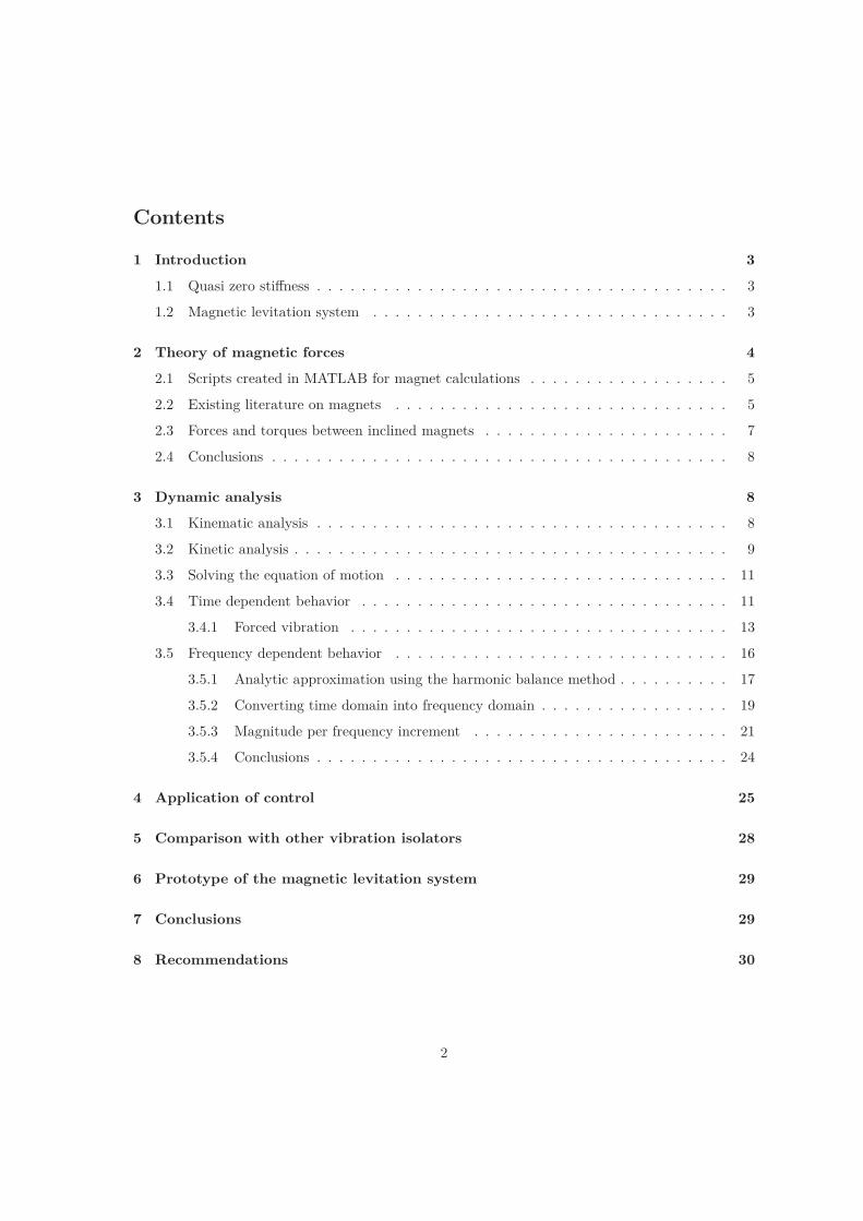
Contents

1 Introduction 3

1.1 Quasi zero stiffness . . . . . . . . . . . . . . . . . . . . . . . . . . . . . . . . . . . . . 3

1.2 Magnetic levitation system . . . . . . . . . . . . . . . . . . . . . . . . . . . . . . . . 3

2 Theory of magnetic forces 4

2.1 Scripts created in MATLAB for magnet calculations . . . . . . . . . . . . . . . . . . 5

2.2 Existing literature on magnets . . . . . . . . . . . . . . . . . . . . . . . . . . . . . . 5

2.3 Forces and torques between inclined magnets . . . . . . . . . . . . . . . . . . . . . . 7

2.4 Conclusions . . . . . . . . . . . . . . . . . . . . . . . . . . . . . . . . . . . . . . . . . 8

3 Dynamic analysis 8

3.1 Kinematic analysis . . . . . . . . . . . . . . . . . . . . . . . . . . . . . . . . . . . . . 8

3.2 Kinetic analysis . . . . . . . . . . . . . . . . . . . . . . . . . . . . . . . . . . . . . . . 9

3.3 Solving the equation of motion . . . . . . . . . . . . . . . . . . . . . . . . . . . . . . 11

3.4 Time dependent behavior . . . . . . . . . . . . . . . . . . . . . . . . . . . . . . . . . 11

3.4.1 Forced vibration . . . . . . . . . . . . . . . . . . . . . . . . . . . . . . . . . . 13

3.5 Frequency dependent behavior . . . . . . . . . . . . . . . . . . . . . . . . . . . . . . 16

3.5.1 Analytic approximation using the harmonic balance method . . . . . . . . . . 17

3.5.2 Converting time domain into frequency domain . . . . . . . . . . . . . . . . . 19

3.5.3 Magnitude per frequency increment . . . . . . . . . . . . . . . . . . . . . . . 21

3.5.4 Conclusions . . . . . . . . . . . . . . . . . . . . . . . . . . . . . . . . . . . . . 24

4 Application of control 25

5 Comparison with other vibration isolators 28

6 Prototype of the magnetic levitation system 29

7 Conclusions 29

8 Recommendations 30

2

1 Introduction

Vibration isolation is of great importance in a lot of fields. Especially for high precision systems, itis desired that unwanted vibration will be isolated so that they have no influence on the performanceof the system and high precision can be maintained. Vibration isolators are systems that are capableof isolating these unwanted vibrations. There are a wide variety of isolators available, which arebased of different principles. This research will focus on a new possible way to isolate vibrations,namely by using a magnetic levitation system. The majority of the research is about analyzingthe theoretical dynamics of such a system in order to gain more understanding in its frequencydependent behaviour and vibration isolation characteristics. Additionally, some research aboutmagnetic forces and a part of the experimental analysis is done.

1.1 Quasi zero stiffness

When the dynamics of a system are being analyzed, the stiffness of the system plays an importantrole. For instance, the natural frequency of a system is partly defined by its stiffness. Consequently,there is a lot of research done on natural frequencies and thus the stiffness of a system, since itcan cause a lot of unwanted vibrations. In order to isolate these unwanted vibrations, one mightwant to decrease the natural frequency that much so it is not close to the operating frequency. Ifa simple undamped mass-spring system is considered, the natural frequency follows from:

ωn =

√

k

m(1)

With k as the stiffness of the spring and m the mass of the system. The natural frequency canthus be reduced by reducing the stiffness of the system. Actually, when there is zero stiffness inthe system, the natural frequency would by zero as well. In the case of the mass-spring system thiswould mean that no energy is transmitted from the base to the mass, which is ideal for the sake ofvibration isolation. The quasi zero stiffness method tries to simulate a zero stiffness by adding apositive stiffness and a negative stiffness to the system. In the formula, this would look like:

ωn =

√

k1 + k2

m(2)

When k1 = −k2, the natural frequency ωn becomes zero. However, this concept comes in practicewith a lot of nonlinearities which is the cause of the research that is done in this area.

1.2 Magnetic levitation system

One way to theoretically obtain quasi zero stiffness is by levitating a mass by two magnets, onerepelling magnet and one attracting magnet. This theory is investigated by dr. Will Robertson asa PhD research [1]. In order to examine his findings more closely, he created a prototype that isable to bring a mass near quasi zero stiffness. A picture of the prototype can be found in figure 1.

3

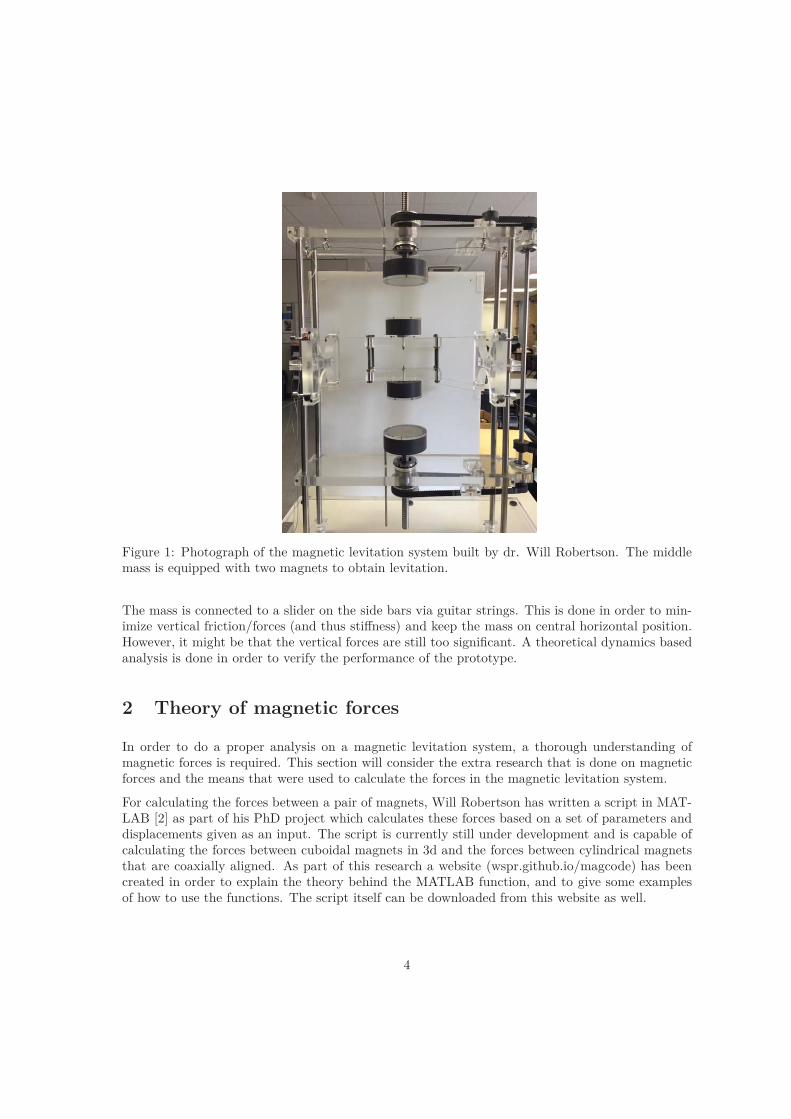
Figure 1: Photograph of the magnetic levitation system built by dr. Will Robertson. The middlemass is equipped with two magnets to obtain levitation.

The mass is connected to a slider on the side bars via guitar strings. This is done in order to min-imize vertical friction/forces (and thus stiffness) and keep the mass on central horizontal position.However, it might be that the vertical forces are still too significant. A theoretical dynamics basedanalysis is done in order to verify the performance of the prototype.

2 Theory of magnetic forces

In order to do a proper analysis on a magnetic levitation system, a thorough understanding ofmagnetic forces is required. This section will consider the extra research that is done on magneticforces and the means that were used to calculate the forces in the magnetic levitation system.

For calculating the forces between a pair of magnets, Will Robertson has written a script in MAT-LAB [2] as part of his PhD project which calculates these forces based on a set of parameters anddisplacements given as an input. The script is currently still under development and is capable ofcalculating the forces between cuboidal magnets in 3d and the forces between cylindrical magnetsthat are coaxially aligned. As part of this research a website (wspr.github.io/magcode) has beencreated in order to explain the theory behind the MATLAB function, and to give some examplesof how to use the functions. The script itself can be downloaded from this website as well.

4

2.1 Scripts created in MATLAB for magnet calculations

Since the calculation of the magnetforces can be quite complex, some extra scrips were created inMATLAB so that certain magnet configurations can be calculated more easier. The following threescripts were created/changed in MATLAB:

1. A lot of systems consider multiple fixed magnets that are used to levitate an other mag-net (floating magnet). To simplify calculations on these systems, another function calledmultimagnetforces.m has been created. This function simply uses the parameters of thefloating magnet and the fixed magnets as an input together with the positions of the magnetsand the displacement of the floating magnet. Additionally, a subfunction drawmagnet.m isused to visualize the magnets in a 3d figure. This way, an easy observation can be madewhether correct input parameters are used.

2. The script magnetforces.m of Will Robertson showed unrealistic results when one has a gapof 0 between two magnets. Some lines have been added to the code that make the face gapsbetween cuboidal magnets eps instead of 0.

3. When cylindrical magnets are not coaxial, another calculation method should be used. Acalculation method that can be used to calculate the forces between cylindrical magnets withan axial offset was developed by John T. Conway [3]. In order to calculate these forces easily,a function has been written in MATLAB. This function is based on the method in which theBessel-Laplace integrals are replaced by their corresponding elliptic integrals and producesthe same results as shown in the paper.

2.2 Existing literature on magnets

Multiple papers are written on the forces that are occurring between magnet pairs. Especially theforce field in different setups of the magnets is of interest since it creates different stiffness fields.

The paper of He Zhang [4] considers a certain magnetic levitation system, see figure 2, with cuboidalmagnets.

Figure 2: Schematic overview of the magnetic levitation system investigated by Zhang.

5

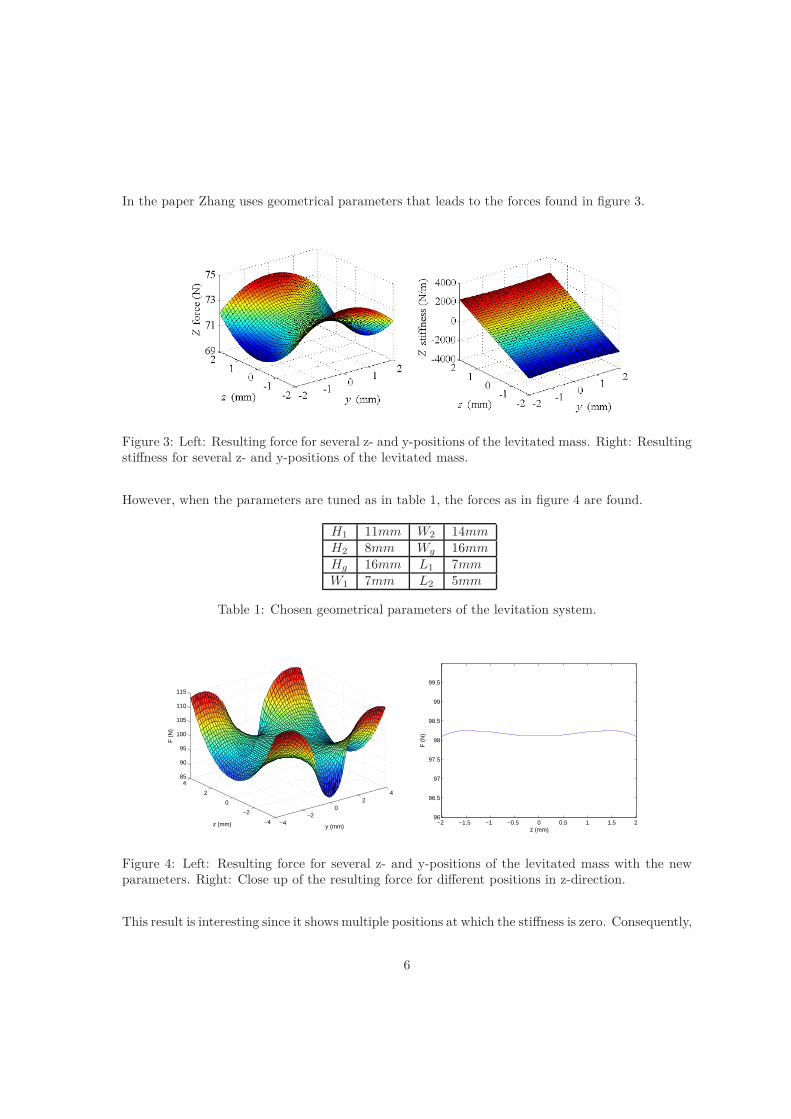
In the paper Zhang uses geometrical parameters that leads to the forces found in figure 3.

Figure 3: Left: Resulting force for several z- and y-positions of the levitated mass. Right: Resultingstiffness for several z- and y-positions of the levitated mass.

However, when the parameters are tuned as in table 1, the forces as in figure 4 are found.

H1 11mm W2 14mmH2 8mm Wg 16mmHg 16mm L1 7mmW1 7mm L2 5mm

Table 1: Chosen geometrical parameters of the levitation system.

−4−2

02

4

−4

−2

0

2

485

90

95

100

105

110

115

y (mm)z (mm)

F (

N)

−2 −1.5 −1 −0.5 0 0.5 1 1.5 296

96.5

97

97.5

98

98.5

99

99.5

z (mm)

F (

N)

Figure 4: Left: Resulting force for several z- and y-positions of the levitated mass with the newparameters. Right: Close up of the resulting force for different positions in z-direction.

This result is interesting since it shows multiple positions at which the stiffness is zero. Consequently,

6

a stable position could be found between two quasi zero stiffness positions which may lead to bettervibration isolation characteristics.

2.3 Forces and torques between inclined magnets

Since there is not really literature available on forces between inclined magnets, this is an interestingcase to consider. The magnetforces function is not able to simulate inclined magnets, but magnetswith an inclined magnetization is possible (that is, changing the ’dir’ vector). By modeling multiplemagnets as one magnet, an inclined magnet of arbitrary shape can possibly be simulated.

Figure 5: Example of multiple magnets being used to simulate an inclined magnet.

0 10 20 30 40 50 60 70 80 90

Angle (degrees)

0

0.005

0.01

0.015

0.02

0.025

0.03

0.035

0.04

0.045

Tor

que

(Nm

)

Torque for different angles

Figure 6: Resulting torque for a row of 3 magnets in different angles.

Figure 6 shows the torque that is caused by a row of 3 magnets when they are rotating around afixed magnet as in figure 5. Something notable in the figure is the nod that can be seen around anangle of 45 degrees.

7

2.4 Conclusions

More insight into magnetic forces has been obtained by looking closer to the existing theory andpapers. Even though the magnetic system that will be considered for the magnetic levitation systemis relatively simple, it is shown that alternative systems are possible as well (e.g. the system given byZhang). Furthermore, the MATLAB function is capable of calculating the forces between magnetsfor a lot of situations but requires some expansion for some special cases. For instance, a functionthat is able to calculate the forces for arbitrary shaped magnets in an arbitrary orientation mightbe convenient for more complex systems. Such a function could be possible by using a group ofsmaller magnets to simulate a larger magnet, as demonstrated in the previous subsection.

3 Dynamic analysis

In order to gain more insight in the behavior of the system, a dynamical analysis has been performedon the system. This analysis is based on a kinematic analysis of the system and the nonlinearequation of motion that follows from the Newton forces balances. By using the equation of motionmore knowledge is gained about the (nonlinear) dynamical behavior of the system for certainparameters.

3.1 Kinematic analysis

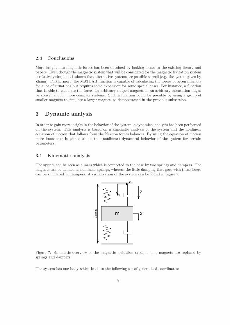
The system can be seen as a mass which is connected to the base by two springs and dampers. Themagnets can be defined as nonlinear springs, whereas the little damping that goes with these forcescan be simulated by dampers. A visualization of the system can be found in figure 7.

m x1

388mm

gx

y

Figure 7: Schematic overview of the magnetic levitation system. The magnets are replaced bysprings and dampers.

The system has one body which leads to the following set of generalized coordinates:

8

q =

x1

y1

θ1

(3)

In which x1, y1 and θ1 are the vertical translation, horizontal translation and the rotation of the bodyrespectively. Since we want to research the behavior in one direction, the prototype is made in such away that y1 and θ1 are constrained as much as possible. In this theoretical model we constrain thesecoordinates as well, i.e. y1 = 0 and θ1 = 0. Considering 3 ∗ [no. of bodies] − [no. of constraints] =DoF we get a 3 ∗ 1 − 2 = 1 DoF system. The independent generalized coordinate is defined as x1

(as can be seen in figure 7).

3.2 Kinetic analysis

In order to obtain the equation of motion of the system, the Newton moment and forces balancesmethod is used. Consider the free body diagram that follows from the system in figure 8.

m x1

Fs1 Fd1mg

Fs2 Fd2

Figure 8: Free body diagram of the magnetic levitation system resulting from the schematic overviewin figure 7.

Taking the force balance in the x-direction gives the following relation:

∑

Fx = mx1 = mg − Fs1(x1) − Fd1(x1, x1) − Fs2(x1) − Fd2(x1, x1) (4)

Note that the magnet forces are nonlinear and dependent on the position of the body. The mag-nitude of these magnetic forces is obtained by using the magnetforces.m MATLAB file created byWill Robertson. This script enables us to calculate the magnetic forces between two, in this casecylindrical, magnets of specified dimensions and types (see table 2). Since the calculation is rathercomplicated, the forces of the magnets (using the specifications of the prototype) are calculated fora set of values of x1 so that a function of x1 can be fitted on these points. Fitting is done usingMATLAB and by using the rational function (p1x2

1 +p2x1 +p3)/(x1 +q1). The following parameterswere found:

9

p1 = 1.395p2 = −416.6p3 = 3.243 · 104

q1 = 31.43

(5)

Magnet 1 Magnet 2Radius (mm) 50 37.5Height (mm) 30 30Grade N35 N42

Table 2: Specifications of the magnets used in the prototype. Magnet 1 refers to the magnetconnected to the base, magnet 2 refers to the magnet connected on the levitated mass.

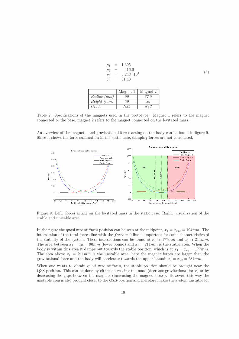
An overview of the magnetic and gravitational forces acting on the body can be found in figure 9.Since it shows the force summation in the static case, damping forces are not considered.

Figure 9: Left: forces acting on the levitated mass in the static case. Right: visualization of thestable and unstable area.

In the figure the quasi zero stiffness position can be seen at the midpoint, x1 = xqzs = 194mm. Theintersection of the total forces line with the force = 0 line is important for some characteristics ofthe stability of the system. These intersections can be found at x1 ≈ 177mm and x1 ≈ 211mm.The area between x1 = xlb = 90mm (lower bound) and x1 = 211mm is the stable area. When thebody is within this area it damps out towards the stable position, which is at x1 = xeq = 177mm.The area above x1 = 211mm is the unstable area, here the magnet forces are larger than thegravitational force and the body will accelerate towards the upper bound; x1 = xub = 284mm.

When one wants to obtain quasi zero stiffness, the stable position should be brought near theQZS-position. This can be done by either decreasing the mass (decrease gravitational force) or bydecreasing the gaps between the magnets (increasing the magnet forces). However, this way theunstable area is also brought closer to the QZS-position and therefore makes the system unstable for

10

even very small excitations. The mass which roughly equals the intersection with the QZS-positionis m = mqzs = 10.4798kg.

3.3 Solving the equation of motion

Rewriting the relation in equation 4 yields the equation of motion of the system:

mx1 + c(x1, x1)x1 + Fs1(x1) + Fs2(x1) = mg (6)

Because very low damping is considered, the system is simplified to a constant damping coefficient:c(x1, x1) = c. However, the equation is still nonlinear because of the nonlinear spring forces. Otherpapers researched similar systems near the QZS-position by considering the Duffing equation [5].Here however, the dynamic behavior of the system will be simulated in time by using integrationmethods which also can give insight in frequency dependent behavior.

Firstly, the equation of motion is transformed into state space in order to obtain two coupledordinary differential equations:

x1 = x1

x1 = − cm

x1 − 1m

[Fs1(x1) + Fs2(x1)] + g(7)

These coupled ODE’s can be solved in MATLAB by using the ode45 function. The dampingparameter c has been chosen at c = 0.0087 so that it is within the order of magnitude correspondingto ζ = 0.02. An exact value of this parameter is not important since it is very small and is frequentlyadjusted to see its effect on the results.

3.4 Time dependent behavior

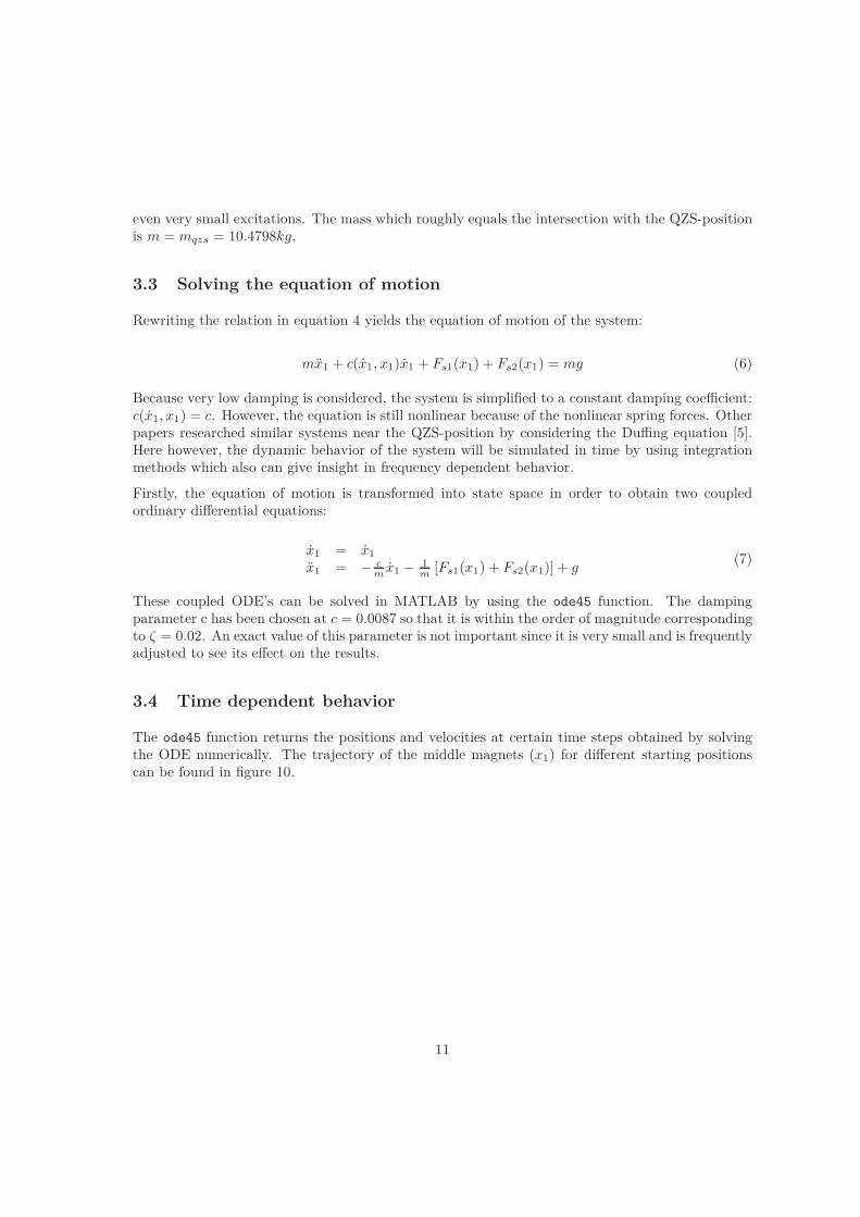
The ode45 function returns the positions and velocities at certain time steps obtained by solvingthe ODE numerically. The trajectory of the middle magnets (x1) for different starting positionscan be found in figure 10.

11

0 20 40 60 80 100 120 140 160 180 200−40

−20

0

20

40

60

80

100

120Trajectory of middle magnets for different initial conditions

Time (s)

Pos

ition

(m

m)

Figure 10: Trajectory of the levitated mass for different initial positions. The used parameters inthis simulation are m = 12kg, c = 0.0087.

As was concluded from figure 9, the system goes unstable for positions above 17mm from theQZS-position (294 + 17 = 211mm). For other starting positions the system starts to oscillate in itsnatural frequency. This natural frequency is dependent on the position x1 since in the linear caseit can be calculated by ωn =

√

(k1 + k2)/m. This demonstrates the idea that a very low naturalfrequency can be found when the system stabilizes near the QZS position. In order to check thatthe simulation is working properly, an overview of the energies is made in figure 11. Apart fromdissipated energy (which should be very low), no energy should flow out of the system, which indeedis true.

12

Figure 11: Kinetic, potential and total energy contained in the system over time. A (nearly, becauseof low damping) constant energy indicates a realistic simulation.

3.4.1 Forced vibration

In order to look at the response of the system for certain frequencies, a harmonic excitation isapplied on the system. Because we want to look at vibration isolation, the base is excited with afunction y1(t) = A sin(ωt). The new system can be visualized as in figure 12.

m x1

gx

y

y (t)1

Figure 12: Schematic visualization of the magnetic levitation system with base excitation.

The equation of motion now becomes:

mx1 + cx1 + Fs1(x1, y1) + Fs2(x1, y1) = mg + cy1(t) (8)

13

With the coupled equations:

x1 = x1

x1 = cm

[y1(t) − x1] − 1m

[Fs1(x1, y1) + Fs2(x1, y1)] + g(9)

Note that the magnet forces are now dependent on both the position x1 and the excitation y1(t).Thetrajectory of the middle magnets (x1) for different starting positions can be found in figure 13.

Figure 13: Trajectory of the levitated mass for different initial positions with base excitation. Theused parameters in this simulation are m = 12kg, c = 0.0087.

When ω is chosen as the natural frequency of the system (ω = ωn) with a certain mass in its stableposition, the system starts to resonate. For a system with mass m = 12kg and a stable position at−17mm from the QZS position, the natural frequency of the linearized system is:

√

√

√

√

(

∂Fs1(x1, y1)

∂x1

∣

∣

∣

∣

x1=−17

+∂Fs2(x1, y1)

∂x1

∣

∣

∣

∣

x1=−17

)

/12 ≈ 0.4Hz (10)

Choosing this frequency as the excitation frequency for the system in its stable position causes thetrajectory which can be found figure 14.

14

Figure 14: Left: trajectory of the levitated mass when the base excites in the natural frequency(ω = ωn, m = 12kg, c = 0.0087). Right: the corresponding phase plot of the undamped system(c = 0).

The pulsating effect can be described as follows:

1. The system is in its stable position (x1 = −17mm) and is excited in its natural frequency atthis position.

2. The system starts to vibrate heavily which causes x1 to fluctuate.

3. The fluctuation of x1 causes a fluctuation in the corresponding natural frequency since it isdependent on x1.

4. The exciting frequency does not correspond with the natural frequency anymore causing thesystem to damp out around its stable position.

5. At this stable position the system starts to resonate yet again, restarting at 1.

This effect can clearly be compared to that of a pendulum, in which the natural frequency iscalculated from the linearized system in its downward stable position. When the excitation of thependulum becomes too large, the linearized natural frequency (obtained by taking the Taylor seriesof the angle around the stable position) is not valid anymore, causing a pulsating effect as well.The Duffing equation, for instance, catches the resulting cubic term arising from taking the Taylorseries and is usually used for hardening springs. The magnetic levitation has softening springs andhas a lot of remaining terms after taking the Taylor series, therefore simulations are done in orderto analyze the system.

The maximum amplitude for a damped system with forced vibration is reached at Ωmax =√

1 − 2ζ2,where Ω = ω

ωn

[6]. Since damping is very low for this system, the term reduces to√

1 − 2 · 0.022 ≈√1 = 1. Thus during resonance the maximum possible amplitude is obtained. Therefore, it is

interesting to analyze at what excitation amplitude the system becomes unstable. For this analysis,the system with an external force applied at the levitated mass is considered, see figure 15.

15

m x1

F(t)

Figure 15: Schematic visualization of the magnetic levitation system with an external applied force.

The external force is defined as F (t) = F sin(ωt). In order to see when the system becomes unstable,simulations are done for different amplitudes F . The relation between the stable position xeq andthe maximum allowed force amplitude F when ω = ωn can be found in figure 16.

0 5 10 150

0.5

1

1.5

2

2.5

3Relation between stability position and allowed force

xeq

(−mm)

F

Data from simulationFitted function

Figure 16: Relation between the equilibrium position and the maximum allowed force (amplitude)applied on the system.

3.5 Frequency dependent behavior

The frequency dependent analysis performed on the system can roughly be divided into two cat-egories: converting the time domain into the frequency domain and an analysis performed perfrequency increment.

16

3.5.1 Analytic approximation using the harmonic balance method

One way to approximate the nonlinear magnetic forces at a certain position is by using the Taylorseries. By applying this method the force will be described as a polynomial in terms of x1. The moreterms are taken into account, the more accurate the approximation will be. We will be applyingthe Taylor series on the total force Ft acting on the initial system, as seen in figure 7. This forcecan be described as:

Ft(x1) = Fs1(x1) + Fs2(x1) − mg (11)

Now the Taylor series up to third order can be applied on this force, applying this at the quasi zerostiffness position xqzs yields:

Ft|x1=xqzs= Ft(0) + F ′

t (0)x1 +1

2F ′′

t (0)x21 +

1

6F ′′′

t (0)x31 (12)

This corresponds to:

Ft|x1=xqzs= (102.7576 − mg) + 0x1 +

1

20.1048x2

1 + 0x31 (13)

Choosing the mass as m = mqzs = 10.4798 leads to the following relation:

Ft|x1=xqzs= 0.0524x2

1 (14)

Which states that the equation of motion has a nonlinear quadratic term. However, since in theabove relation the stiffness is zero and we want to analyze the system at a stable position xeq

approaching the QZS position, the following relation is used:

Ft|x1=xeq= γx1 + κx2

1 (15)

In which γ and κ can be calculated by taking the Taylor series at the stable position. In order tocalculate the response, we consider the system when the levitated mass is excited with an externalforce, see figure 15. The external force is defined as F (t) = F cos(ωt). We define the natural

frequency of the linear system, ωn =√

km

, as the 0th order solution ω0. This leads to the following

equation of motion at the stable position in dimensionless form:

x + βx + γx1 + κx21 = F cos(Ωτ) (16)

With β = 2ζ, Ω = ωω0

, τ = ω0t, F = FC

Where C is a constant that is yet to be determined by a comparison with the simulation performedin the time domain. A solution to the above equation of motion can be found by using the harmonicbalance method, which solves the equation by using a trial function with sines and cosines. Thesolution in this report follows the method as explained in [7]. First, the trial solution for x isdefined:

17

x = Z + a sin(Ωτ) + b cos(Ωτ)x = aΩ cos(Ωτ) − bΩ sin(Ωτ)x = −aΩ2 sin(Ωτ) − bΩ2 cos(Ωτ)

(17)

−aΩ2 sin(Ωτ) − bΩ2 cos(Ωτ) + aβΩ cos(Ωτ) − bβΩ sin(Ωτ) + γZ,+aγ sin(Ωτ) + bγ cos(Ωτ) + (κZ)2 + 2Zκ2a sin(Ωτ) + 2Zκ2b sin(Ωτ),

+2κ2ab sin(Ωτ) cos(Ωτ) + 12 κ2(a2 + b2) − 1

2 κ2(a2 − b2) cos(2Ωτ) = F sin(Ωτ)(18)

Where the identities sin2(Ωτ) = 1 − cos2(Ωτ) and cos2(Ωτ) = 12 − 1

2 cos(2Ωτ) are used. By ignoringhigher order terms, the following coefficients are found for the sine, cosine and constants:

γZ + (κZ)2 + 12 κ2(a2 + b2) = 0

−aΩ2 − bβΩ + aγ + 2Zκ2a = F−bΩ2 + aβΩ + βγ + 2Zκ2b = 0

(19)

By defining r =√

a2 + b2, the first equations yields:

r2 = −2( γ

κ2Z + Z

)

(20)

The second and third can be solved in matrix vector form:

[

−Ω2 + γ + 2Zκ2 −βΩβΩ −Ω2 + γ + 2Zκ2

]

−1F0

=

ab

(21)

Leading to the solutions:

a =−F(Ω2

−2κ2Z−γ)(Ω2−2κ2Z−γ)2+(βΩ)2 b = −F βΩ

(Ω2−2κ2Z−γ)2+(βΩ)2(22)

Combining these definitions with the definition r =√

a2 + b2 yields:

F 2 = −2( γ

κ2Z + Z

) [

(

Ω2 − 2κ2Z − γ)2

+ (βΩ)2]

(23)

Now, since the amplitude A is defined as A = r + Z, the amplitude at a certain frequency andexcitation force can be calculated by choosing F , Ω, γ and κin equation 23 and solve for Z. Thisresults in a set of solutions that are all part of one nonlinear response of the system. Figure 17shows an example of the frequency response for the stable position xeq = −10mm.

18

0.4 0.6 0.8 1 1.2 1.4 1.6 1.8 2−60

−40

−20

0

20

40

60

Ω

Am

plitu

de

Frequency response for xeq

= −10mm, ζ = 0.02, F^ = 1.5

1234

Figure 17: Left: Responses calculated by using MATLAB. Right: Relevant shapes which forms theactual response.

3.5.2 Converting time domain into frequency domain

The trajectory for a single frequency input computed in the previous section can be convertedinto the frequency domain in order to get more insight in the frequencies ‘hidden’ in the resultantdynamics. MATLAB offers several functions to do this. In this research, three functions were used:tfestimate (transfer function estimate), fft (Fast Fourier Transform) and pwelch (Welch’s powerspectral density estimate). The first function, tfestimate, tries to extract a frequency responsefunction from the input and the resulting output of the system. We consider the again the systemexcited at the base, as shown in figure 12. Since the base is externally excited, the input is definedas y(t). The output is the trajectory of the system x(t). In order to gain as much informationabout the system as possible, a random input is considered. This is done by transforming the setof equations to the following four coupled differential equations:

x1 = x1

x1 = cm

[y1 − x1] − 1m

[Fs1(x1, y1) + Fs2(x1, y1)] + gy1 = y1

y1 = A [0.5 − rand(1)]

(24)

The acceleration of the input is thus randomly defined by rand(1) which gives a random numberbetween 0 and 1. The results of tfestimate can be found in figure 18, the values for the parametersused are shown in table 3. Here, also a comparison is made with pwelch applied on both the input

and the output and subsequently related to each other via T =√

pxx

pyy

.

19

10−3

10−2

10−1

100

101

102

10−5

10−4

10−3

10−2

10−1

100

101

102

Frequency (Hz)

Mag

nitu

de (

dB)

Frequency response using tfestimate and pwelch, m=12kg

TFestimatePwelch

10−4

10−3

10−2

10−1

100

101

102

10−6

10−5

10−4

10−3

10−2

10−1

100

101

102

Frequency (Hz)

Mag

nitu

de (

dB)

Frequency response using tfestimate and pwelch with simulink, m=12kg

TF (acc)TF (vel)TFwelch (acc)TFwelch (vel)

Figure 18: Left: frequency dependent behavior of the magnetic levitation system by using ode45in combination with both tfestimate and pwelch and considering the velocities. Right: the samesimulation executed by using simulink with both the velocities and the accelerations.

m 12kg T max 1000sc 0.0087 ∆T 0.1A 0.5 ∆F 0.1

Table 3: Parameter values used in the simulations in figure 18.

A clear peak can be found around the resonance frequency ωn = 0.4Hz. However, another smallerpeak can be found at around twice the natural frequency. This phenomenon can be seen as perioddoubling. The results of fft can be found in figure 19 and the results of the pwelch method canbe found in figure 20. These last two figures shows the fft and pwelch method applied on thetrajectory (output) found when exciting the system in its natural frequency, as in figure 14.

Figure 19: Frequency dependent behavior by using the fast fourier transform method on the systemexcited by a single frequency.

20

Figure 20: Frequency dependent behavior by using Welch’s power spectral density estimate on thesystem excited by a single frequency.

In figure 19 and 20 peaks can clearly be found towards 0Hz, around 0.06Hz and around 0.11Hz.The one towards zero indicates the large pulsating movements, which occurs every 190 seconds andis 1/290 = 0.0034Hz. 0.06Hz indicates the vibrations within the pulses, which occurs 17 timesevery 290 seconds and is about 17/290 = 0.058Hz. The small disturbance at 0.12Hz indicates thatthere should be another periodic movement within the smaller vibrations.

3.5.3 Magnitude per frequency increment

A very direct method in calculating the frequency response is by considering a certain excitationfrequency, calculate the trajectory and calculate the magnitude of the response by root meansquaring the trajectory and dividing it by the input (y1(t)), and increase the step n. Mathematicallythis can be shown as follows:

Tn =

√

x21,n

√

y21,n

n = 1, 2, 3.. (25)

Increasing the frequency a little bit each step results in a frequency response graph. The result fordifferent masses can be seen in figure 21. The used parameters are shown in table 4.

21

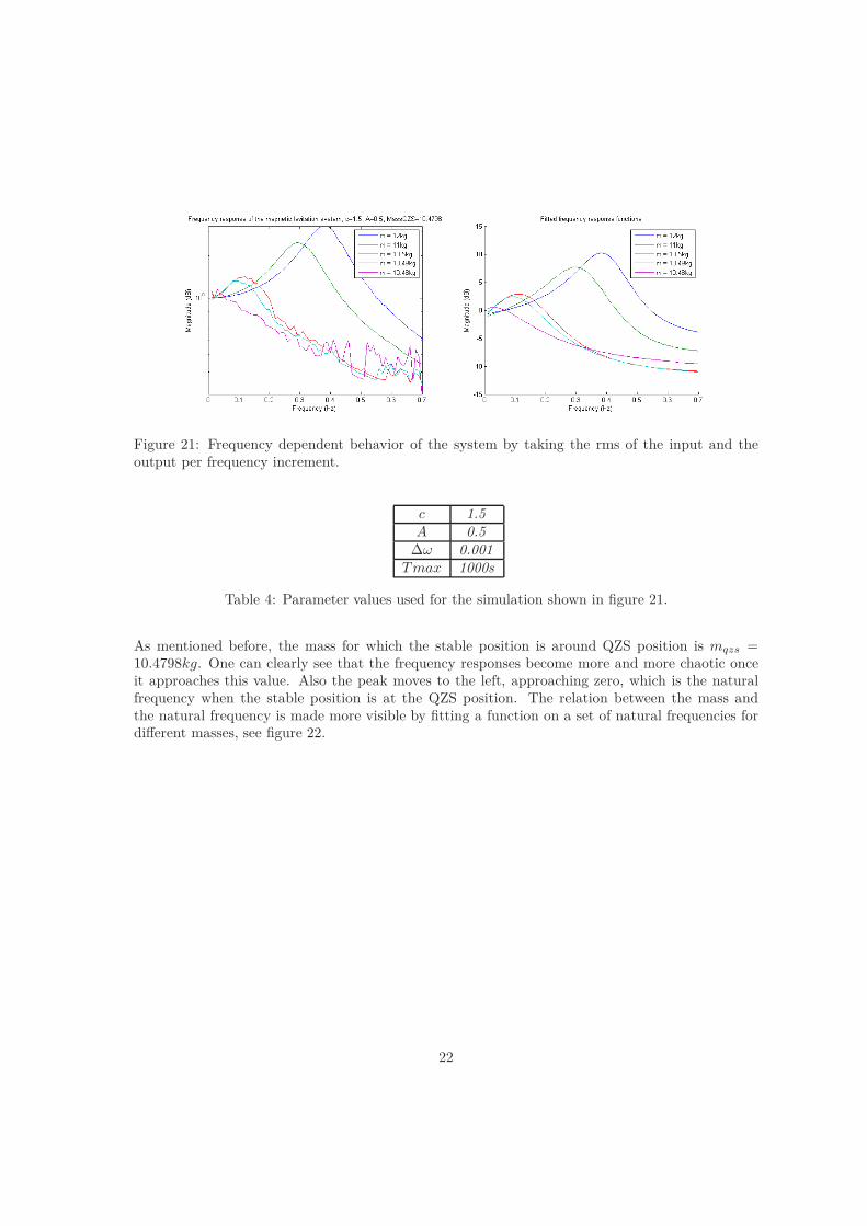
Figure 21: Frequency dependent behavior of the system by taking the rms of the input and theoutput per frequency increment.

c 1.5A 0.5

∆ω 0.001T max 1000s

Table 4: Parameter values used for the simulation shown in figure 21.

As mentioned before, the mass for which the stable position is around QZS position is mqzs =10.4798kg. One can clearly see that the frequency responses become more and more chaotic onceit approaches this value. Also the peak moves to the left, approaching zero, which is the naturalfrequency when the stable position is at the QZS position. The relation between the mass andthe natural frequency is made more visible by fitting a function on a set of natural frequencies fordifferent masses, see figure 22.

22

Figure 22: Relation between the mass of the levitated middle magnets and the natural frequencyof the system.

These simulations were done for a relatively high damping in order to make sure that the simulationworks properly and in order to get fairly smooth results. When the damping is lowered to thepreviously stated value of c = 0.0087, the response becomes as in figure 23.

Figure 23: Frequency dependent behavior for the levitation system with low damping c = 0.0087,m = 11.5kg.

A small nonlinearity can be observed in the peak, it tends to bend a bit to the left. This ischaracteristic for systems with softening springs. For systems with hardening springs, e.g. Duffingequation, the peak bends to the right side.

To validate and compare the results, the transmissibility of the system is considered as well. Con-

23

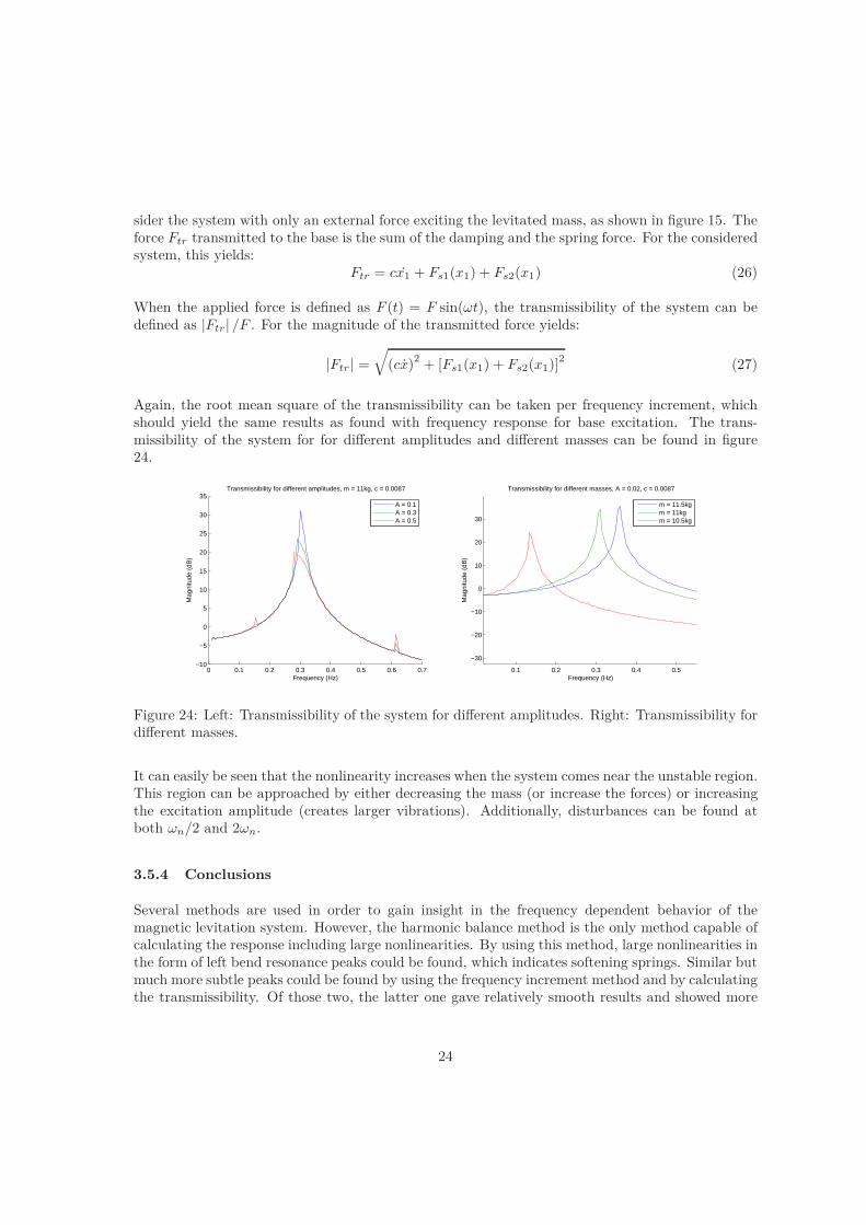
sider the system with only an external force exciting the levitated mass, as shown in figure 15. Theforce Ftr transmitted to the base is the sum of the damping and the spring force. For the consideredsystem, this yields:

Ftr = cx1 + Fs1(x1) + Fs2(x1) (26)

When the applied force is defined as F (t) = F sin(ωt), the transmissibility of the system can bedefined as |Ftr| /F . For the magnitude of the transmitted force yields:

|Ftr | =

√

(cx)2

+ [Fs1(x1) + Fs2(x1)]2

(27)

Again, the root mean square of the transmissibility can be taken per frequency increment, whichshould yield the same results as found with frequency response for base excitation. The trans-missibility of the system for for different amplitudes and different masses can be found in figure24.

0 0.1 0.2 0.3 0.4 0.5 0.6 0.7−10

−5

0

5

10

15

20

25

30

35

Frequency (Hz)

Mag

nitu

de (

dB)

Transmissibility for different amplitudes, m = 11kg, c = 0.0087

A = 0.1A = 0.3A = 0.5

0.1 0.2 0.3 0.4 0.5

−30

−20

−10

0

10

20

30

Transmissibility for different masses, A = 0.02, c = 0.0087

Frequency (Hz)

Mag

nitu

de (

dB)

m = 11.5kgm = 11kgm = 10.5kg

Figure 24: Left: Transmissibility of the system for different amplitudes. Right: Transmissibility fordifferent masses.

It can easily be seen that the nonlinearity increases when the system comes near the unstable region.This region can be approached by either decreasing the mass (or increase the forces) or increasingthe excitation amplitude (creates larger vibrations). Additionally, disturbances can be found atboth ωn/2 and 2ωn.

3.5.4 Conclusions

Several methods are used in order to gain insight in the frequency dependent behavior of themagnetic levitation system. However, the harmonic balance method is the only method capable ofcalculating the response including large nonlinearities. By using this method, large nonlinearities inthe form of left bend resonance peaks could be found, which indicates softening springs. Similar butmuch more subtle peaks could be found by using the frequency increment method and by calculatingthe transmissibility. Of those two, the latter one gave relatively smooth results and showed more

24

insight in the relations between nonlinearity, mass/magnet-gaps and force amplitudes. Additionally,period doubling and period halfing phenomena were observed when calculating the transmissibility.

The source of these period doubling and halfing is unknown. It occurs in both the transmissibilityanalysis and the tfestimate and pwelch analyses.

The big nonlinearities as shown in the analytic solution are practically not really possible, since thesystem becomes already unstable when the peak is slightly bend. This can also be seen in figure 24at the transmissibility for F = 0.5.

4 Application of control

The fact that bringing the stable position towards the QZS position increases the risk of an unstablesystem is a problem. In this chapter research is done on the behavior of the system when it isforced to stay at the QZS position by means of control. The control will be applied according tothe ’backstepping method’ as explained by Mahmoud in his paper [8]. This method is based on theLyapunov stability criterium and the focus is to design a closed-loop system with proper stabilityproperties by using a so called control Lyapunov function.

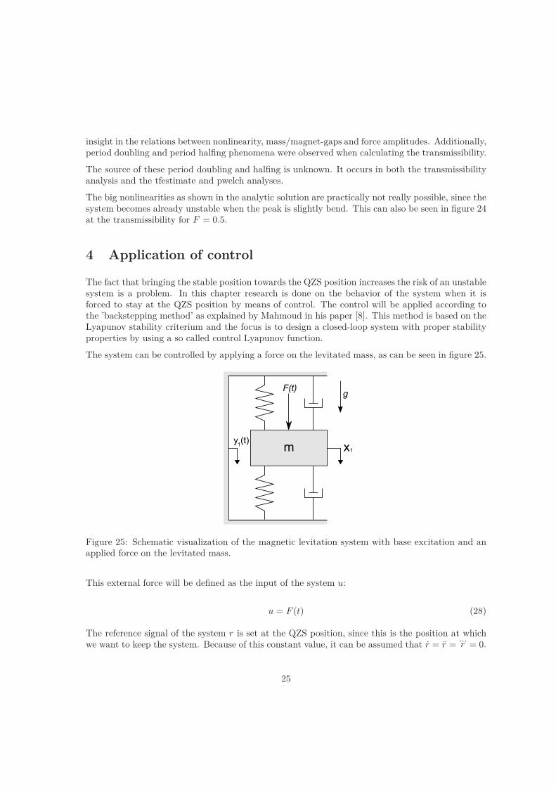
The system can be controlled by applying a force on the levitated mass, as can be seen in figure 25.

m x1

g

y (t)1

F(t)

Figure 25: Schematic visualization of the magnetic levitation system with base excitation and anapplied force on the levitated mass.

This external force will be defined as the input of the system u:

u = F (t) (28)

The reference signal of the system r is set at the QZS position, since this is the position at whichwe want to keep the system. Because of this constant value, it can be assumed that r = r =

...r = 0.

25

Again the equation of motion is considered as two coupled differential equations, but this timex = x1 and x = x2 is used as a notation for clarity.

x1 = x2

x2 = cm

[Aω cos(ωt) − x2] − 1m

[Fs1(x1, y1) + Fs2(x1, y1)] + g + u(29)

The first error variable will be defined as:

z1 = x1 − r (30)

Taking the time derivative and considering that r = 0, the following relation yields as well:

z1 = x2 (31)

A simple clf for this equation is V = 12 z2

1 with the corresponding time derivative:

V = z1z1 = z1x2 (32)

The first stabilizing function can be chosen as:

xdes2 = −c1z1 ≡ α c1 > 1 (33)

Substituting in the clf yields:

V = −c1z21 ≤ −z2

1 (34)

The second error variable can now be defined as:

z2 = x2 − α (35)

This yields the following set of differential equations:

z1 = z2 + αz2 = − c

m(z2 + α) − 1

m[Fs1(z1, y1) + Fs2(z1, y1)] + g + c

my1(t) + u + c1 (z2 + α)

(36)

Consequently, the new clf becomes:

V =1

2z2

1 +1

2z2

2 (37)

The derivative can be expanded as follows:

26

V = z1z1 + z2z2

= z1 (z2 + α) + z2

cm

[y1(t) − (z2 + α)] − 1m

[Fs1(z1, y1) + Fs2(z1, y1)] + g + um

+ c1 (z2 + α)

= z1α + z2

z1 − cm

[y1(t) − (z2 + α)] − 1m

[Fs1(z1, y1) + Fs2(z1, y1)] + g + um

+ c1 (z2 + α)

≤ −z21 + z2

z1 − cm

[y1(t) − (z2 + α)] − 1m

[Fs1(z1, y1) + Fs2(z1, y1)] + g + um

+ c1 (z2 + α)

≤ −z21 − z2

2

(38)

The input of the system u can now be chosen conveniently in order to obtain a closed loop system.Let u be:

u = c [(z2 + α) − y1(t)] − z1m + Fs1(z1, y1) + Fs2(z1, y1) − mg − mc1 (z2 + α) − mc2z2 (39)

Which results in the system:

z1 = z2 − c1z1

z2 = −c2z2 − z1(40)

In matrix-vector form this can be written as:

z =

[

−c1 1−1 −c2

]

z1

z2

(41)

When this matrix is Hurwitz, i.e. the real part of the eigenvalues is negative, stability is fulfilled:

s1,2 = −c1 + c2

2± 1

2

√

(c1 − c2)2 − 4 (42)

With the defined error variables z1 and z2 the input u (external force) is defined with the parametersc1 and c2 left as new unknowns. These parameters can be chosen conveniently (i.e. both positive)in order to obtain stability. Implementing the differential equations 29 in the simulation, choosingc1 = c2 = 0.5 and solving using ode45 yields the trajectory in time domain as shown in figure 26.

27

0 5 10 15 20 25 30

Time (s)

-20

-15

-10

-5

0

5

Pos

ition

(m

m)

Trajectory of the middle magnets with base excitation

c1 = c2 = 0.5c1 = c2 = 1c1 = c2 = 1.5

Figure 26: Trajectory of the levitated mass when controlled using the backstepping method.

It can be seen that the position remains stable at the QZS position after around 13 seconds. Whenhigher values are chosen for c1 and c2, this time decreases and the QZS position is reached earlier.

5 Comparison with other vibration isolators

The magnetic levitation system is capable of lowering the natural frequency drastically, which isinteresting for the sake of vibration isolation. There are currently a lot of vibration isolators on themarket. In this section a brief comparison is made with a couple of these vibration isolators.

Natural frequency range (Hz) 0-0.4Loads (kg) 10.48-12Maximum allowed excitation amplitude (mm) 0.0001-2.5Transmissibility at resonance (dB) ~20

Table 5: Found characteristics for the magnetic levitation system as a vibration isolator.

A popular vibration isolator with a good performance is the air table. This isolator typically has anatural frequency around 2-2.5Hz.

Another interesting example of a vibration isolator is the negative stiffness isolator. This isolatoris based on a similar principle as the quasi zero stiffness method and are usually built by minusK technologies. These systems are able to bring the natural frequency towards 0.5 Hz. Since thisnatural frequency is relatively low, this type of isolator is usually applied on nano-equipment.

In table 5 can be seen that the magnetic levitation system is able to obtain even lower naturalfrequencies. However, the excitation amplitude is constrained to very low values.

28

6 Prototype of the magnetic levitation system

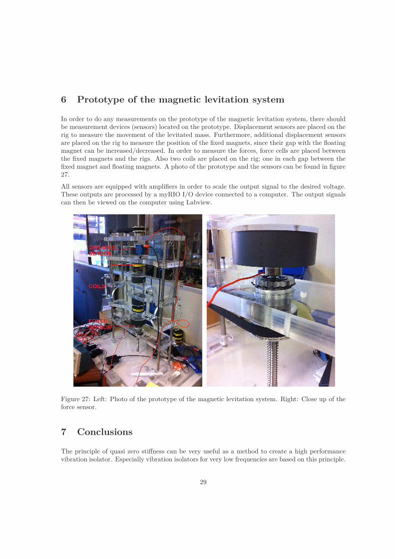
In order to do any measurements on the prototype of the magnetic levitation system, there shouldbe measurement devices (sensors) located on the prototype. Displacement sensors are placed on therig to measure the movement of the levitated mass. Furthermore, additional displacement sensorsare placed on the rig to measure the position of the fixed magnets, since their gap with the floatingmagnet can be increased/decreased. In order to measure the forces, force cells are placed betweenthe fixed magnets and the rigs. Also two coils are placed on the rig; one in each gap between thefixed magnet and floating magnets. A photo of the prototype and the sensors can be found in figure27.

All sensors are equipped with amplifiers in order to scale the output signal to the desired voltage.These outputs are processed by a myRIO I/O device connected to a computer. The output signalscan then be viewed on the computer using Labview.

Figure 27: Left: Photo of the prototype of the magnetic levitation system. Right: Close up of theforce sensor.

7 Conclusions

The principle of quasi zero stiffness can be very useful as a method to create a high performancevibration isolator. Especially vibration isolators for very low frequencies are based on this principle.

29

Usually these systems try to reach quasi zero stiffness by a system of mechanical springs, creatingpositive and negative stiffnesses. However, a system using magnetic levitation to reach quasi zerostiffness might be an interesting alternative. By analyzing the dynamics of such a system in theory,more insight is gained in its nonlinearities and capabilities.

By using pairs of coaxial cylindrical magnets, a relatively simple magnetic levitation system isobtained. This system is able to reach quasi zero stiffness in theory, but becomes unstable with anysmall disturbance. From different theoretical methods, more insight is gained into the dynamicaland frequency dependent behavior of the system. It is found that the system indeed shows nonlinearbehavior with spring softening. By using the theoretical model, one can predict which frequencyranges can be isolated and for which amplitudes the system becomes unstable. However, the isolatedfrequency range depends on the maximum force amplitude that is applied on the system. The lowerthe frequency one wants to isolate, the lower the allowed force amplitude. This relation is foundvia simulations and approximated as:

Fmax = 0.011 · x2eq + 0.00016 · xeq (43)

A possible solution to get rid of the risk on instability with larger amplitudes is by applying controlusing the backstepping theory. However, such an application of control might in practice have badconsequences on the performance of the vibration isolation system. Other methods for increasingthe maximum amplitude, such as applying a linear increasing force on the levitation system, doesnot seem to to have the desired effect.

8 Recommendations

Some recommendations can be done based on the done research. Especially since the work is partof a bigger research within obtaining quasi zero stiffness using magnetic levitation.

1. The theoretical model needs to be further verified and compared to the prototype. In orderto do this, the prototype needs to be completed entirely. Furthermore, some basic exactmeasurements of the weight, magnet forces (using the force sensors) and other parametershave to be done and (if required) adjusted in the theoretical model. When this is done, aniterative process between the prototype and the theoretical model can be done for an thoroughanalysis of the system. These findings could be presented in a paper.

2. The frequency response found by using the harmonic balance method might need some evalu-ation of a specialist. Altough the overall shape of the graph and the influence of the differentparameters are probably correct, there is still some uncertainties with respect to the instability.That is, for which force amplitudes does the system becomes unstable? Also some verificationis required. Especially the equation in dimensionless form might need some attention.

3. It could be useful to dome some tests with the prototype and control. For instance, applyingbackstepping or similar methods. A linear increasing force was found to be not useful, butmight still be interesting to consider to apply on the prototype.

30

4. A fairly simple system with two pairs of coaxial cylindrical magnets was considered. As seenin the magnet analysis, some other configurations give interesting force fields on the levitatedmass which might be more beneficial. Some of these configurations could be elaborated moreto see what it does around quasi zero stiffness and when it becomes unstable.

References

[1] Robertson, W. (2013). Modeling and design of magnetic levitation systems for vibration isola-tion. PhD thesis. School of Mechanical Engineering, The University of Adelaide.

[2] Robertson, W. Calculating forces between magnets using MATLAB.https://github.com/wspr/magcode.

[3] Conway, J. (2013). Forces Between Thin Coils With Parallel Axes Using Bessel Functions. IEEETransactions on Magnetics, 49(9), pp.5028-5034.

[4] Zhang, H., Kou, B., Jin, Y., Zhang, H. and Zhang, L. (2014). Research on a Low Stiffness PassiveMagnetic Levitation Gravity Compensation System with Opposite Stiffness Cancellation. IEEETransactions on Magnetics, 50(11), pp.1-4.

[5] Xu, D., Yu, Q., Zhou, J. and Bishop, S. (2013). Theoretical and experimental analyses of anonlinear magnetic vibration isolator with quasi-zero-stiffness characteristic. Journal of Soundand Vibration, 332(14), pp.3377-3389.

[6] Schilder, J. (2014). Dynamics 2. Faculty of Engineering Technology, University of Twente.

[7] Virgin, L. (1988). On the harmonic response of an oscillator with unsymmetric restoring force.Journal of Sound and Vibration, 126(1), pp.157-165.

[8] Mahmoud, N. (2003). A Backstepping Design of a Control System for a Magnetic LevitationSystem. MSc thesis. Department of Electrical Engineering, Linköping University.

31

Appendix

In this appendix, the code is shown of some calculations that are used in the research in order toprovide more understanding.

In order to calculate the forces between the magnets, the script magnetforces.m is used. Below isa piece of code that shows how to calculate forces from this script by using specified magnets, andhow to fit a curve on the found forces.

% Magnet 1 :r1 = 0 . 0 5 0 ; % radius , metresh1 = 0 . 0 3 0 ; % height , metresgrade1 = ’N35 ’ ;% Magnet 2 :r2 = 0 . 0 7 5 / 2 ; % radius , metresh2 = 0 . 0 3 0 ; % height , metresgrade2 = ’N42 ’ ;% Displacement :gap_max = 0 . 2 ; % metresface_gap = l i n s p a c e (0 , gap_max , 2 0 0 ) ; % 200 data po i ntsd i s p l = face_gap + h1/2 + h2 /2 ;

% Cal cu l ate f o r c e s :f c y l = magnetforces ( . . .s t r u c t ( ’ grade ’ , grade1 , ’ dim ’ , [ r1 h1 ] , ’ d i r ’ , [ 0 0 −1]) , . . .s t r u c t ( ’ grade ’ , grade2 , ’ dim ’ , [ r2 h2 ] , ’ d i r ’ , [ 0 0 1 ] ) , . . .d i sp l ’ ∗ [ 0 0 1 ] . . .) ;

% Plot f o r c e sf i g u r e (1) ; c l f ; hold a l lx = 1000∗ face_gap ;p l o t ( x , f c y l ( 3 , : ) , ’ o ’ ) ;x l a b e l ( ’ Face gap , mm’ ) ; y l a b e l ( ’ Force , N ’ ) ;

% Fit curveFO = f i t ( x ’ , f c y l ( 3 , : ) ’ , ’ rat21 ’ , ’ S tar tPo i nt ’ , [ 2 −45 2000 9 ] ) ;va l ues = c o e f f v a l u e s (FO) ;p1 = va l ues (1) ; p2 = va l ues (2) ; p3 = va l ues (3) ; q1 = va l ues (4) ;F = ( p1∗x . ^2 + p2∗x + p3 ) . / ( x + q1 ) ;p l o t ( x , F) ;l egend ( ’ Resu l t s from magnetforces .m’ , ’ F i t ted curve ’ ) ;

A part of the MATLAB code that simulates the system without excitation is shown below. It showsthe implementation of the coupled differential equations that follows from the equation of motion,and how it is linked with the ODE solver ode45.

% Solve system of d i f f e r e n t i a l equat i ons us ing ode45opt i ons = odeset ( ’ Events ’ , @StateSpaceSimpleEvent ) ;[T,X,TE,YE, IE ] = ode45 ( @StateSpaceSimpleFunction , [ 0 , maxTime ] , [ x0 , 0 ] , opt i o ns ) ;

f u n c t i o n X = StateSpaceSimpleFunction ( t , x )% x i s an array o f l ength 2 that s t o r e s the data .% x (1) = displacement% x (2) = v e l o c i t y

32

g l o b a l c m Fs1 Fs2 gx1 = x (1) ; %r e q u i r e d to eva l uate Fs1 and Fs2

% Coupled d i f f e r e n t i a l equat i onsX( 1 , 1 ) = x (2) ;X( 2 , 1 ) = −(c/m) ∗x (2)−eva l ( Fs1 ) /m−eva l ( Fs2 ) /m+g ;

end

f u n c t i o n [ value , i s t e r m i n a l , d i r e c t i o n ] = StateSpaceSimpleEvent ( t , x )% Locate the time when middle magnets reach the upper / lower bound% and stop i n t e g r a t i o n .value = [ x (1) −90 x (1) −284] ; %detect x = upper / lower boundi s t e r m i n a l = 1 ; %stop the i n t e g r a t i o nd i r e c t i o n = [−1 1 ] ; %d e f i n e d i r e c t i o n

end

Below the function is shown that is used by the ode45 function when the backstepping method isapplied.

f u n c t i o n X = BacksteppingFunction ( t , x )% x i s an array o f l ength 2 that s t o r e s the data .% x (1) = displacement% x (2) = v e l o c i t yg l o b a l m g Fs1 Fs2 c A r omegax1 = x (1) ; %r e q u i r e d to eva l uate Fs1 and Fs2

% Set backstepping parametersc1 = 0 . 5 ; c2 = 0 . 5 ;z1 = x (1)−r ;alpha = −c1 ∗ z1 ;z2 = x (2)−alpha ;ydot = A∗omega∗ cos ( omega∗ t ) ;

% Def ine inputu = c ∗( z2+alpha )−z1 ∗m+eva l ( Fs1 )+eva l ( Fs2 )−g∗m−c∗ydot−m∗c1 ∗( z2+alpha )−c2 ∗ z2 ∗m;

% Coupled d i f f e r e n t i a l equat i onsX( 1 , 1 ) = x (2) ;X( 2 , 1 ) = −(c/m) ∗x (2)−eva l ( Fs1 ) /m−eva l ( Fs2 ) /m+g+u/m;

end

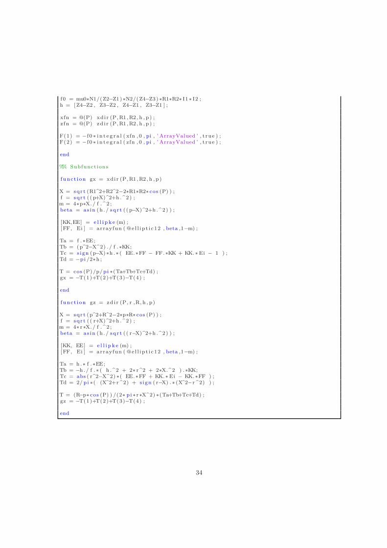
Next, the code is shown that is able to calculate the forces between cylindrical magnets positionedwith a coaxial offset.

f u n c t i o n F = cyl_calc_noncoaxial_w(R1 , R2 , Z1 , Z2 , Z3 , Z4 , N1 , N2 , I1 , I2 , p)% C a l c u l a t e s the f o r c e s between c y l i n d r i c a l magnets with an a x i a l o f f s e t ,% the method used to c a l c u l a t i n g these f o r c e s o r i g i n a t e from the paper o f% John T. Conway and r e p l a c e s the Besse l −Laplace i n t e g r a l s o f the o r i g i n a l% method with t h e i r cor r espond i ng e l l i p t i c i n t e g r a l e x p r e s s i o n s .%% Equations s i m p l i f i e d mar g i na l l y by WSPR ( hence may no l onger be c o r r e c t ) .

mu0 = 4∗ pi ∗10^( −4) ;

33

f 0 = mu0∗N1/( Z2−Z1 ) ∗N2/( Z4−Z3 ) ∗R1∗R2∗ I1 ∗ I2 ;h = [ Z4−Z2 , Z3−Z2 , Z4−Z1 , Z3−Z1 ] ;

xfn = @(P) xd i r (P, R1 , R2 , h , p ) ;z f n = @(P) z d i r (P, R1 , R2 , h , p ) ;

F(1) = −f 0 ∗ i n t e g r a l ( xfn , 0 , pi , ’ ArrayValued ’ , t r ue ) ;F(2) = −f 0 ∗ i n t e g r a l ( zfn , 0 , pi , ’ ArrayValued ’ , t r ue ) ;

end

%% Subfunctions

f u n c t i o n gx = xdi r (P, R1 , R2 , h , p )

X = s q r t (R1^2+R2^2−2∗R1∗R2∗ cos (P) ) ;f = s q r t ( ( p+X)^2+h . ^ 2 ) ;m = 4∗p∗X. / f . ^ 2 ;beta = as i n ( h . / s q r t ( ( p−X)^2+h . ^ 2 ) ) ;

[KK,EE] = e l l i p k e (m) ;[ FF, Ei ] = arrayfun ( @ e l l i p t i c 1 2 , beta ,1−m) ;

Ta = f . ∗EE;Tb = ( p^2−X^2) . / f . ∗KK;Tc = s i gn (p−X) ∗h . ∗ ( EE. ∗FF − FF. ∗KK + KK. ∗ Ei − 1 ) ;Td = −pi /2∗h ;

T = cos (P) /p/ p i ∗(Ta+Tb+Tc+Td) ;gx = −T(1)+T(2)+T(3)−T(4) ;

end

f u n c t i o n gz = z d i r (P, r ,R, h , p)

X = s q r t ( p^2+R^2−2∗p∗R∗ cos (P) ) ;f = s q r t ( ( r+X)^2+h . ^ 2 ) ;m = 4∗ r ∗X. / f . ^ 2 ;beta = as i n ( h . / s q r t ( ( r−X)^2+h . ^ 2 ) ) ;

[KK, EE] = e l l i p k e (m) ;[ FF, Ei ] = arrayfun ( @ e l l i p t i c 1 2 , beta ,1−m) ;

Ta = h . ∗ f . ∗EE;Tb = −h . / f . ∗ ( h . ^2 + 2∗ r ^2 + 2∗X. ^2 ) . ∗KK;Tc = abs ( r^2−X^2) ∗( EE. ∗FF + KK. ∗ Ei − KK. ∗FF ) ;Td = 2/ p i ∗( (X^2+r ^2) + s i gn ( r−X) . ∗ (X^2−r ^2) ) ;

T = (R−p∗ cos (P) ) /(2∗ pi ∗ r ∗X^2) ∗(Ta+Tb+Tc+Td) ;gz = −T(1)+T(2)+T(3)−T(4) ;

end

34