EXAMINING THE ROLE OF DISCHARGE GAS AND …davincarter.com/Davin/M._Sc._files/Davin Carter, M. Sc.,...

EXAMINING THE ROLE OF DISCHARGE GAS AND VAPOUR INTRODUCTION FOR

ATMOSPHERIC PRESSURE PHOTOIONIZATION MASS SPECTROMETRY

by

Davin Martin Richard Carter

B. Sc., Carleton University, 2006

A THESIS SUBMITTED IN PARTIAL FULFILLMENT OF

THE REQUIREMENTS FOR THE DEGREE OF

MASTER OF SCIENCE

in

THE COLLEGE OF GRADUATE STUDIES

(Chemistry)

THE UNIVERSITY OF BRITISH COLUMBIA

(Okanagan)

June 2012

© Davin Martin Richard Carter, 2012

ii

Abstract

The recent introduction of commercial Atmospheric Pressure PhotoIonization (APPI) sources

for use on Liquid Chromatography-Mass Spectrometry (LCMS) instruments has expanded

the range of analytes that can be analyzed to include non-polar compounds. The two

commercial photon sources use a low pressure krypton discharge lamp that selectively

ionizes many classes of analytes but not common solvents. This thesis explores two

hypotheses; (a) that ionization can be independent of discharge gas type and (b) that vapours

of solid samples can be ionized and rapidly analyzed by mass spectrometry.

To explore the effect of discharge gas on ionization, a novel atmospheric pressure discharge

lamp was constructed. Helium, nitrogen, argon, hydrogen, oxygen, carbon dioxide, and

compressed air were evaluated as discharge gases to generate photons that would induce

photoionization in naphthalene as a representative polycyclic aromatic hydrocarbon. Photon

emission spectra of argon, helium, hydrogen, oxygen and nitrogen were characterized and

found to be consistent to reference spectra. Calibration curves were constructed for

naphthalene and compared to a calibration curve obtained using a commercial (PhotoMate,

Syagen Inc.) photoionization lamp. The custom made discharge lamp was slightly more

sensitive and gave mass spectra comparable to the commercial lamp leading to the

conclusion that ionization was independent of discharge gas type.

iii

Under the second objective, an innovative way to introduce vapours from solid samples was

developed. Small amounts of solid crystal sample were heated to produce vapours that were

then photoionized. Mass spectra were collected on a number of polycyclic aromatic

compounds and metal containing organic compounds. Collision induced dissociation was

used to characterize specific analytes of interest.

The ability to use a variety of discharge gases for photoionization lowers the cost of

construction and improves the ruggedness of photoionization ionization sources. The ability

to quickly characterize solid samples has a range of applications including rapid confirmation

of synthetic chemistry reactions, quality assurance in pharmaceutical production, detection of

drugs of abuse and detection of chemical warfare agents.

iv

Preface

This thesis is in part the result of collaborations with the Institute for Pure and Applied Mass

Spectrometry at the University of Wuppertal, Germany. Design, fabrication and evaluation of

the Lightning Ion Source was a joint effort of Dr. Hendrik Kersten and myself. I primarily

designed, fabricated and evaluated the TAVI apparatus with some assistance from Dr.

Kersten.

Portions of this work have been presented at the American Society for Mass Spectrometry

conference in 2010 and the International Conference on Analytical Sciences and

Spectroscopy in 2009.

v

Table of Contents

Abstract …………………………………………………………….……………………… ii

Preface ……………………………………………………………….……………………. iv

Table of Contents …………………………………………………….……………………. v

List of Tables ……………..………………………………………….…….………..……. viii

List of Figures ………………………………………………………….…….……………. ix

Acknowledgements …………………………………………………….…………………. xi

Chapter 1: Introduction …………………………………………….….……….………… 1

1.1 History of photon generation .……………………………..…….……………. 2

1.2 Krypton photon generation ……………………….…….….…………………. 4

1.3 History of photoionization mass spectrometry …………….………………… 5

1.4 Discharge windows ………………………………………….………….……. 8

1.5 Photoelectron spectroscopy ………………………………….………….……. 9

1.6 Mechanisms of photoionization .…………………………….………….……. 11

1.6.1 Mechanism of direct photoionization ………………….………….…… 11

1.6.2 Mechanisms of secondary ionization leading to [M+H]+ .….….…….… 12

1.6.3 Dopants .…….…………………………………………….…….……… 15

1.7 Structure determination …………………….………….…….….….………… 16

1.8 Ambient ionization ………….……….…….…………………….…………… 17

1.9 Hypothesis .…….……….…………………………….………………………. 19

Chapter 2: Experimental ………………………………………….………………………. 20

2.1 Introduction …………………………………………….………….…………. 20

vi

2.2 Lightning Ion Source ………………………………………………………… 20

2.2.1 Instrumentation …………………………….……….…….…………… 22

2.2.1.1 Mass spectrometer ………………………………………… 22

2.2.1.2 Optical spectrometer …………………………………...…. 23

2.2.1.3 Liquid chromatography ……………….……….…….……. 24

2.2.2 Chemicals and discharge gases …………………….……………….…. 24

2.2.3 Standard solutions ………………………………………….…….……. 24

2.3 Using atmospheric pressure photoionization to characterize vapours ………. 25

2.3.1 Instrumentation ………………………………………………………… 27

2.3.2 Chemicals ……………………………………………………………… 28

Chapter 3: Results ……………………………………………………………….………. 29


3.1.1 Emission spectra ………………………………………………………. 29

3.1.2 Mass spectra generated with Lightning Ion Source …………………… 36

3.1.3 Calibration curves …….………….……………………………………. 39

3.1.3.1 Krypton discharge lamp …………………………….…….. 41

3.1.3.2 Air discharge lamp …………………………………..……. 43

3.1.3.3 Helium discharge lamp ………………….……….….……. 45

3.1.3.4 Nitrogen discharge lamp .…….…….……..………………. 47

3.1.3.5 Argon discharge lamp …………….….…………………. 49

3.1.3.6 Hydrogen discharge lamp ………….…………….….……. 51

3.1.3.7 Oxygen discharge lamp …………….………………….…. 53

3.1.3.8 Carbon dioxide discharge …………………………………. 55

vii

3.1.3.9 Analysis of variance ………………………………………. 57

3.2 Thermally Assisted Vapour Introduction results ………………………….… 60

3.2.1 TAVI mass spectra ………………………………………………….… 60

Chapter 4: Discussion ……………………………………………………………………. 69


4.1.1 Emission spectra ………………………………………………………. 70

4.1.2 Mass spectra …………………………………………………………… 71

4.1.3 Calibration curve ………………………………………………………. 71

4.2 Demonstrating APPI for characterization of synthetic products ………….…. 72

Chapter 5: Conclusions …………………………………………………….…….….…… 75

5.1 Summary …………………….…………….………………….……………… 75

5.2 Lightning Ion Source …………………………………………………………. 75

5.3 Thermally Assisted Vapour Introduction ……………………………….……. 77

References ……………………………………………….………….……….………….… 78

viii

List of Tables

Table 1: Lightning Ion Source mass spectrometer conditions ……………………..……. 23

Table 2: TAVI source Mass spectrometer conditions ………………….……….…..…… 27

Table 3: Comparison of the predicted NIST reference emission profile of argon to

experimental values ………………………………………………………………….…… 30

Table 4: Comparison of the predicted NIST reference emission profile of hydrogen to


Table 5: Comparison of the predicted NIST reference emission profile of helium to


Table 6: Comparison of the predicted NIST reference emission profile of oxygen to


Table 7: Comparison of the predicted NIST reference emission profile of nitrogen to


Table 8: Comparison of peak area of duplicate pyrene signals from the commercial lamp

and argon Lightning Ion Source ….……….…….………….……….……….….……..… 37

Table 9: Comparison of duplicate measurements of peak height of commercial lamp and

argon Lightning Ion Source for 17-α-hydroxyprogesterone …………….………………. 39

Table 10: Figures of merit of naphthalene to discharge gas ……….…….……………… 40

Table 11: Peak area as a function of naphthalene concentration ….………….…….…… 41

Table 12: Peak area as a function of naphthalene concentration …….……….……….… 43

Table 13: Peak area as a function of naphthalene concentration ……….……….…….… 45

Table 14: Peak area as a function of naphthalene concentration ……….……….………. 47

Table 15: Peak area as a function of naphthalene concentration …….……….……….… 49

Table 16: Peak area as a function of naphthalene concentration …….…….…….……… 51

Table 17: Peak area as a function of naphthalene concentration …….……….…….…… 53

Table 18: Peak area as a function of naphthalene concentration …….……….…….…… 55

Table 19: ANOVA of response to concentration ………………………….………….…. 58

ix

List of Figures

Figure 1: Relation between photon energy and discharge gas …………….…….…….… 10

Figure 2: Emco powered Lightning Ion Source ………………………………….……… 21

Figure 3: TAVI apparatus ………………………………………………………….……. 26

Figure 4: Mass spectra of pyrene by commercial kr and lab built lamp ….…….…….… 36

Figure 5: Mass spectra of 17-α-hydroxyprogesterone by commercial kr and the LIS .… 38

Figure 6: Analytical calibration curve of naphthalene to krypton discharge .…....…..…. 42

Figure 7: Residuals of naphthalene linear regression for krypton discharge .….….….… 42

Figure 8: Analytical calibration curve of naphthalene to air discharge .…….……..…… 44

Figure 9: Residuals of naphthalene linear regression for air discharge …….….….….… 44

Figure 10: Analytical calibration curve of naphthalene to helium discharge .…….……. 46

Figure 11: Residuals of naphthalene linear regression for helium discharge ..…...….…. 46

Figure 12: Analytical calibration curve of naphthalene to nitrogen discharge .….…..…. 48

Figure 13: Residuals of naphthalene linear regression for nitrogen discharge .….….….. 48

Figure 14: Analytical calibration curve of naphthalene to argon discharge ….…...……. 50

Figure 15: Residuals of naphthalene linear regression for argon discharge .….….….…. 50

Figure 16: Analytical calibration curve of naphthalene to hydrogen discharge .….….… 52

Figure 17: Residuals of naphthalene linear regression for hydrogen discharge ….….…. 52

Figure 18: Analytical calibration curve of naphthalene to oxygen discharge .….……… 54

Figure 19: Residuals of naphthalene linear regression for oxygen discharge …...…..…. 54

Figure 20: Analytical calibration curve of naphthalene to carbon dioxide discharge ...... 56

Figure 21: Residuals of naphthalene linear regression for carbon dioxide discharge ...... 56

Figure 22: TAVI ms of ferrocene ………………………………………………………. 60

Figure 23: CID ms/ms spectra of ferrocene …………………………………………..… 61

Figure 24: TAVI mass spectra of naphthalene …………………………………………. 62

Figure 25: TAVI ms of biphenyl ……………………………………………………….. 63

Figure 26: TAVI ms of Cr(acac)3 …………………………………………………….…. 64

x

Figure 27: TAVI ms/ms of Cr(acac)3 …………………………………………………… 65

Figure 28: TAVI ms of LG113 …………………………………………………….……. 66

Figure 29: TAVI spectrum of LG113 …………………………………………………… 67

Figure 30: TAVI spectra of LG159 ……………………………………………………… 68

xi

Acknowledgements

A sincere thank you to Dr. Rob O'Brien for supervising and guiding me through this process.

Throughout the process Rob has given me incredible insights and advice.

I wish to thank the many people who have helped and encouraged me throughout this

research. The staff of the UBC Okanagan Chemistry Department were of great help during

my thesis. I’d like to acknowledge a passionate educator, Judit Moldovan, who was an

inspiration for educators. The time and useful feedback from my thesis committee has been

incredibly useful throughout this project. Dave Arkinstall was a great sounding board and

wealth of experience. Life long friends, Dr. Thorsten Benter and Dr. Hendrik Kersten of the

Institute for Pure and Applied Mass Spectrometry from the University of Wuppertal,

Germany provided great discussions and ideas for this research.

I'd like to acknowledge the support my parents and brother have given over the years. Sadly,

my father in law, who had a keen curiosity and interest in science, passed away days before

my defense. The patience, support and support of my wife made all this work possible.

This work was made possible by instrumentation grants from the Western Economic

Diversification fund and The British Columbia Knowledge Development fund.

1

Chapter 1: Introduction

Photons were one of the first energy sources used to generate ions for mass spectrometry

(Ditchburn and Arnot, 1929). Despite that fact, photoionization sources were not widely used

for quantitative mass spectrometry until the year 2000 when Atmospheric Pressure

Photoionization (APPI) sources were introduced for use on Liquid Chromatography-Mass

Spectrometer (LCMS) instruments (Robb et al., 2000; Syage et al., 2000). There are two

distinct patented commercially available sources: The PhotoMate™ source based on the

Syage patent (Syage et al., United States, 5,808,299, 1998) is available from Syagen

Technology and the PhotoSpray™ (Robb et al., United States, 6,534,765 B1, 2003), is

available from MDS Sciex. In both cases, a low pressure krypton discharge lamp is used as

the photon source.

The APPI-LCMS systems that are currently in operation are used primarily to measure

analytes in solution. It has been demonstrated that the analyte vapors in the absence of

solvents, analyzed by APPI, primarily produced molecular ion mass spectra (Syage, J.,

2004). From this we generated a hypothesis that examining the vapors from materials

produced by synthetic organic processes could provide key diagnostic information. The

validity of this hypothesis will also be explored in this work. We also investigate the use of

an alternate discharge lamp to generate photons for an APPI-LCMS system.

This introduction will begin with background material on the history of photon generation

and also include an explanation of photon generation. A summary of the history of

2

photoionization mass spectrometry is then provided, then a description of optical filters and

an alternate technique, photoelectron spectroscopy, that provides insight into photoionization

mechanisms. These lead into a summary of the current understanding of reaction

mechanisms occurring in APPI – MS. Our understanding of these mechanisms enabled us to

hypothesize that APPI MS could be extremely useful for structure determination for synthetic

compounds and this led to the development of the heated probe introduction approach that

we will also cover at the end of this introduction. A brief summary of rapid ambient

ionization analysis techniques is then offered.

1.1 History of photon generation

The production of photons is a fundamental part of photoionization and has been studied for

over 100 years (Lyman, 1906). The photoemission spectra of many gases have shown

extensive emission lines (Lyman, 1906; Hopfield, 1930, Tanaka et al., 1958). Many of the

original measurements of photoemission spectra were carried out with open flow discharge

cells operating near one atmosphere with large monochromators and large arrays of

photographic plates (Lyman and Saunders, 1926; Hopfield, 1930).

Electrical discharges of many gases have been found to produce photons over a wide range

of energies. Beginning in 1906, a number of researchers measured the emission wavelengths

of hydrogen and helium. A significant number of hydrogen line emissions were identified

from 100 nm to 185 nm (Lyman, 1906; Lyman, 1924; Millikan and Bowen, 1924; Banning,

1942; Poschenrieder and Warneck, 1968) and major emission lines of helium were found at

3

25.63, 30.36 and 58.44 nm with continuous emission between 60.0 nm and 100.0 nm

(Hopfield, 1930; Huffman et al., 1965).

Other elements have been found to have numerous emission lines. For example, over eighty

emission lines were attributed to carbon within the wavelength range of 36 nm to 180 nm,

fourteen to nitrogen between 66 nm and 150 nm and sixty eight to oxygen ranging from 14

nm and 134 nm (Millikan and Bowen, 1924). Xenon was found to have a broad continuous

discharge from 150 to 210 nm (Wilkinson and Tanaka, 1955; Tanaka, 1955, Huffman et al.,

1965). Krypton was found to have a continuum emission starting at its resonance line at

123.6 nm extending to 180.0 nm (Tanaka, 1955; Huffman et al., 1965). The argon continuum

was found to range from 105.0 to 155.0 nm (Lyman, 1925; Huffman et al., 1965; Tanaka,

1955). It is especially noteworthy that electrical discharges in air have been found to release

photons of continuous energy between 45 nm and 240 nm (Sabine, 1939) corresponding to

energies between 27.5 eV and 5.1 eV, which covers the full range of photoionization. These

and other reports from the literature show that many discharge gases produce photons of

varying energies.

Emission spectra have been found to be dependent on several parameters; gas pressure within

the discharge chamber, electrode gap, electrode material and trace contaminants

(Druyvestevyn and Penning, 1940; Huffman et al.,1965; Tanaka, 1955; Tanaka et al., 1958).

Varying pressure has been found to broaden emission lines, shift emission lines and cause

asymmetry in emission lines (Lalos and Hammond, 1961).

4

While much of the literature focuses on the strongest emission lines, emission spectra have

been shown to have broad ranges of photon wavelengths (Tanaka et al., 1958). It has been

shown that hydrogen, krypton, argon and helium have broad emission peaks that are 30 nm

to 50 nm in width.

1.2 Krypton photon generation

The most commonly used photoionization lamp is a krypton discharge lamp. As with all such

discharge sources, the photon energies and related wavelengths are characteristic of the

discharge gas used (Gross and Caprioli, 2007). In the initial publications describing APPI

LCMS (Robb et al., 2000, Syage et al., 2000) it was stressed that the selection of lamp

wavelength was critically important. The krypton discharge lamp was selected because its

emission spectra allowed ionization of an important range of analytes. In a low pressure

krypton discharge lamp, the most significant photons produced have energies of 10.0 eV

(80%) or 10.6 eV (20%) (Borsdorf et al., 2007) that are sufficient to ionize important analyte

classes such as steroids and other aromatic analytes but below the ionization potential of

most LC solvents.

The mechanism for photon emission within a discharge lamp begins with a discharge of

electrons from the electrode surface through the low pressure gas contained within the lamp.

Typical voltages present within these devices are approximately 400 volts. The energy from

the discharge of electrons through the low pressure krypton gas generates a population of

krypton cations and free electrons. These rapidly recombine to form excited state krypton

5

atoms that relax to common metastable states (Kr*). These states are called metastable states

because they are known to persist for long periods of time since they are in triplet spin state

while the ground state is a singlet state. These metastable states do eventually relax back to

the ground state and release photons of well defined energies. An analogous process occurs

in all noble gasses. This process of photon is described in Equations 1a through 1c below.

e- + Kr → Kr+ + 2e- Equation 1a Kr+ + e- → Kr* Equation 1b Kr* → Kr + hν Equation 1c

1.3 History of photoionization mass spectrometry

Photoionization mass spectrometry began in 1929 (Ditchburn and Arnot, 1929) and has

examined variety of discharge gases to produce photons with a wide range of energies

(Webb, United States Patent, 3,521,054, 1970). The first generation of photo-induced ions

was first reported in 1929 by Ditchburn and Arnot, who used a magnetic sector mass

spectrometer to detect potassium photo-induced ions (Ditchburn and Arnot, 1929). Lossing

and Tanaka (1956) published mass spectra of parent ions of acetone, anisole and various

hydrocarbons generated with a sector mass spectrometer using a krypton discharge lamp with

a lithium fluoride window. The essentially monochromatic nature of photons from their lamp

offered sharp separation of ion-forming processes and great simplification of photoionization

spectra over traditional electron impact that often exhibited many fragment peaks and weak

molecular ion peak (Lossing and Tanaka, 1956). Herzog and Marmo (1957) described a

hydrogen discharge and lithium fluoride window that produced very simple mass spectra

6

usually consisting of just the molecular ion peak. Jensen and Libby (1964) constructed a

simple helium discharge lamp that used tungsten wires as electrodes. They investigated

discharge current, electrode temperature (up to 1660 k) and charge density around the

electrodes at different orientations (Jensen and Libby, 1964). In 1966, photoionization mass

spectra with little fragmentation was observed and it was found that the parent or “parent

plus one” was the sole contributor to the mass spectrum (Poschenrieder and Warneck, 1966).

Using different discharge chamber capillaries, made of quartz (emitting a continuous flux)

and ceramic (emitting a pulsed discharge), coupled with a monochrometer, emission bands

from various gases with a resolution of 0.1 eV were produced (Poschenrieder and Warneck,

1966). By selection of discharge gas, the wavelength of resulting photons could be controlled

to selectively ionize the gases of trace analyte while not ionizing interfering gases. This

allowed for analysis of trace gases like N2O that would have been masked by CO2 and

allowed separation of CO from N2 (Poschenrieder and Warneck, 1966). The elimination of a

heated filament that may cause thermal degradation was seen as an additional benefit of

photoionization (Poschenrieder and Warneck, 1968). In 1966, Brion reported a windowless

photoionization source for use with a solid sample probe that showed large increases in

relative abundance of molecular ion in comparison to traditional electron impact ionization

source (Brion, 1966). In a 1969 patent, Yamane described a photoionization detector that

used a discharge in helium, argon or hydrogen to measure gases and vapours (Yamane,

United States Patent, 3,454,828, 1969). A 1970 patent from NASA used a continuous

wavelength argon source and a diffraction grating to provide a selectable wavelength photo

ionization source (Webb, United States Patent, 3,521,054, 1970). A patent was issued to

Driscoll for a selective photoionization source (Driscoll, United States Patent, 40,359/72,

7

1972). Using gases ranging from hydrogen, xenon, argon or krypton resulted in photons of

energies between 9.25 to 15.55 eV were transmitted either through a lithium or magnesium

fluoride window. The first report of a photoionization detector (PID) coupled to GC was in

the 1970’s when Driscoll et al. replaced their traditional FID detector with a PID. In their

work, a variety of hydrocarbons were ionized via a sealed UV lamp that emitted 10.20 eV

photons from a hydrogen discharge through a magnesium fluoride window (Driscoll and

Warneck, 1973). Driscoll recognized that fragmentation of analytes and interfering matrix

could be minimized by controlling photon energy (Driscoll and Warneck, 1973). Unlike,

conventional electron impact mass spectrometry at the time, they were able to differentiate

oxygen gas from methanol by selecting a photon wavelength that ionized methanol but not

oxygen (Driscoll and Warneck, 1973). In 1991, Revel’skii et al. proposed using

photoionization mass spectrometry without separation of multi component mixtures.

Examining low molecular weight compounds, the group examined esters, alkanes, alkenes,

ketones and aromatic hydrocarbons using photons from a krypton discharge lamp at 10.2 eV

and detected them with a mass spectrometer (Revel’skii et al. 1991). The literature contains

extensive work developing and using photoionization prior to 2000.

8

1.4 Discharge windows

Discharge windows allow selective transmission of certain light wavelengths while holding

back the discharge gas and the complex discharge induced chemistry (ions and metastables)

(Druyvesteyn, 1940; Kiser, 1965). When lithium fluoride is used as a discharge window,

photons of wavelength greater than 105 nm (11.8 eV) can pass through to reach the analytes

(Gerisimova, 2006). The transmission properties of various materials has been studied for

over 100 years (Lyman. 1906).

The study of optical transmission of a variety of substances began with Lyman. Windows of

fluorite (CaF2) were used by Lyman in his 1906 examination of hydrogen discharge lines

where he observed no emission lines less than 120 nm were transmitted through the fluorite.

He wrote that the “discovery of some substance transparent to light of the very shortest

wave-length known to exist would be an important step” (Lyman, 1906). Further

investigation found that fluorite allows transmission of photons on energies 115 nm to 700

nm (Gerasimova, 2006). Examinations into the UV-optical properties of sodium and

potassium date back to 1919 when Wood found that thin layers of potassium did not transmit

any visible light but transmitted at UV wavelengths less than 360 nm (Wood, 1919). The

optical properties of lithium fluoride in the extreme ultraviolet were first reported in 1927

(Gyulai, 1927). A more detailed study compared lithium fluoride to calcium fluorite (CaF2)

and found that LiF was more transparent in the far UV (Schneider, 1936) transmitting light of

wavelengths down to 110 nm, (Gyulai, 1927; Schneider, 1936; Milgram and Givens, 1962;

Patterson and Vaughn, 1963; Gerasimova, 2006). Later, the UV cutoff was further refined to

9

105 nm (11.8 eV) (Kato and Nakashima,1960; Kato, 1961). It was noted that there should be

sufficient separation between electrical discharges and LiF windows to avoid discolouration

of the window (Schneider, 1936). Magnesium fluoride has also been used for photo

ionization lamps (Robb, United States Patent, 6,534,765 B1, 2003) and has been reported to

be slightly more tolerant of harsh conditions and transmit photons of 110.0 - 136.0 nm

wavelength (Duncanson and Stevenson, 1958; Gerasimova, 2006). Aluminum thin layers

have been used as filters and windows in the extreme UV (Hass and Tousey, 1959; Madden

and Canfield, 1961). Thin aluminum foil transmits up to 100 nm (Jenson and Libby, 1964;

Walker et al., 1958; Kinsinger et al., 1972; Sieck and Gordon, 1973).

1.5 Photoelectron spectroscopy

Photoelectron spectroscopy (PES) measurements offer information about atomic and

molecular energy levels (Nordling et al., 1957; Frost et al., 1966) and provide important

insights into photoionization. PES describes that if photon energy is in excess of the

ionization potential, ionization will likely occur as described by Equation 2.

Eelectron = hν - E ionization potential Equation 2: Electron energy

PES measures the energy of electrons emitted from material exposed to high energy photons.

The kinetic energy of photoelectrons can be measured by an electrostatic kinetic energy

analyzer coupled to an electron multiplier. Typically, a microwave powered helium discharge

is used to produce monochromatic photons at 58.4 nm or 21.2 eV (Kinsinger et al., 1972).

10

The energy of a photon is related to Plank’s constant (h), the speed of light (c) and its

wavelength (ν) and the energy in excess of the ionization potential leaves in the departing

electron as given by Equation 1. The generation of photoelectrons was first observed by

Heinrich Hertz in 1887 and explained by Albert Einstein in quantum mechanical terms when

he developed the theory that light was composed of discrete quanta, or photons (Einstein,

1905).

It has been shown that electrons of differing binding energies can be removed by high energy

photons (Kinsinger et al., 1972). In larger molecules, the release of electrons of differing

ionization potentials gives rise to ionization continua with many peaks (Al-Joboury and

Turner, 1963; Clark and Frost, 1967).

Figure 1: Relation between photon energy and discharge gas

11

All of the of the noble gases listed in Figure 1, with the exception of xenon, have sufficient

energy to ionize benzene. Photons derived from a helium discharge have the greatest energy

at 19.8 eV and could induce various cationic states. Photons from krypton discharges are

used in commercial APPI discharge lamps as their energy is below most solvents but above

most analyte molecules (Robb et al., 2000). The photon cut off for lithium fluoride crystals is

indicated in Figure 1 to highlight that lithium fluoride is not useful for photons with energy

greater than 11.8 eV (or less than 105 nm).

1.6 Mechanisms of photoionization

Ions found in photoionization mass spectra can generally be attributed to two distinct but

related mechanisms. From photoelectron theory, direct photoionization would be the

expected to only produce molecular ion and a free electron. However, the enhancement of the

signal through the addition of dopants leads to the generation of non-molecular ions such as

(M+H)+ that are a clear demonstration of chemical processes are involved (Syage, 2004) or

in other words photoinduced chemical ionization.

1.6.1 Mechanism of direct photoionization

By definition, primary photoionization leads exclusively to a molecular cation M+, and direct

PI spectra are dominated by a molecular cation peak (Gross et al., 2007) that is produced as

described in Equation 3. Unlike other ionization methods, the photoionization process does

not lead to deposition of excess energy into the molecule. From photoelectric theory, all of

12

the excess photon energy is deposited into the departing electron (Equation 3) and thus the

only excess energy that the molecular ion will have is a function of the geometric differences

between the neutral and the specific cation state produced. In many cases there is very little

difference in ground state geometries and so little fragmentation of parent ions is observed.

This makes APPI a soft ionization technique resulting in predominately molecular ions

(Syage et al., 2004). As photoionization involves interactions of photons with compounds,

gas phase acid base chemistry plays a much smaller role as compared to ESI and APCI (Bos

et al., 2006).

M + hν → M+ + e- Equation 3: Photoionization

1.6.2 Mechanisms of secondary ionization leading to [M+H]+

The photoionization mechanism described by the previous equation can only produce simple

molecular ions or fragments but it has been widely noted that a majority of ions generated by

the commercial APPI sources are [M+H]+ rather than M+ (Syage et al., 2004). The formation

of [M+H]+ has been demonstrated to be a result of “chemical ionization” that involves

solvent or matrix species in some form but the mechanism of ionization is disputed (Kaupilla

et al., 2002; Syage et al., 2004).

It is highly probable that the reactions that lead to [M+H]+ are the result of a chemical

ionization process involving solvent or other matrix species that have been chemically

activated by photon absorption or reactions resulting from photon absorption leading to

13

Photon Induced Chemical Ionization (PICI) (Kersten et al., 2009). Nevertheless, the specific

mechanisms of formation of [M+H]+ are not fully understood and several different

mechanisms have been proposed (Kaupilla et al., 2002; Syage et al., 2004; Kersten et al.,

2009). One hypothesis proposed is analyte cation formation followed by hydrogen

abstraction from protic solvents (Syage et al., 2004). Kaupilla, in 2002, examined ionization

mechanisms of APPI and concluded that [M+H]+ is most likely the result of proton transfer

from the protonated solvent to the analyte. Interestingly, Kauppila disregarded direct

photoionization for the formation of M+ and believed that M+ is formed primarily by charge

exchange between C7H8+ and the analyte (Kauppila et al., 2002). Others hypothesize that the

significant amount of neutral radicals are produced by the krypton discharge lamp and that

these could have a significant influence on APPI spectra (Kersten et al., 2009).

By examining several naphthalenes of varying proton affinities Kauppila et al. (2002) found

that toluene radical cation was formed by photoionization as described in Equation 4. If the

proton affinity of the solvent was greater than benzyl radical, proton transfer is possible

leading to possible dopant- solvent- analyte cascade of proton transfer. Two different

mechanisms are described below, both resulting in the formation of [M+H]+.

Formation of [A+H]+ via dopant charge transfer (Kauppila et al., 2002)

hν + C7H8 → C7H8+ + e- Equation 4: Toluene dopant radical cation formation

C7H8+ + M → C7H7

+ MH+ Equation 5: Proton transfer between dopant & analyte

14

Formation of [A+H]+ via dopant charge transfer to solvent to analyte (Kauppila et al., 2002)

hν + C7H8 → C7H8+ + e- Equation 6: toluene dopant radical cation formation

C7H8+ + S → C7H7

+ SH+ Equation 7: proton transfer between dopant & solvent

SH+ + M → MH+ + S Equation 8: formation of AH+ via solvent charge transfer

In contrast, Syage et al. (2004) reported direct analyte photoionization followed by hydrogen

abstraction from solvent to form [M+H]+. By comparing spectra of pure vapours to solvated

samples and comparing spectra of protic and aprotic solvents, Syage et al. (2004) concluded

that the solvents were the source of protons. The mechanism of [M+H]+ formation was

assessed in a comparison of mass spectra of pure vapours to the spectra of analytes dissolved

in various solvents and found that M+ dominated in headspace vapours (Syage et al., 2004).

The presence of [M+H]+ ions only in solvated samples indicates the involvement of the

solvent in formation of [M+H]+. Further supporting that the proton came from the solvent

was evidence that [M+H]+ formed in the presence of protic solvents while [M+H]+ wasn’t

observed to the same extent with aprotic solvents. Examination of the ratio of [M+H]+/M+

over a range of concentrations provided evidence that self reaction was not significant

reaction pathway (Syage et al., 2004). Further examination indicated the formation of

[M+H]+ in the ionization chamber rather than inside the mass spectrometer. It was also

demonstrated that the [M+H]+/M+ ratio is highly dependent on experimental parameters that

affect ion residence time in the ionization chamber. Modelling studies indicated that proton

affinity was a good proxy for the degree of hydrogen addition, whereas ionization energy

was found not to be a good indicator (Syage et al., 2004).

15

M + hν → M+ + e- Equation 2: Photoionization

M+ + S → MH+ + S-H Equation 9: PICI proton abstraction from protic solvent

1.6.3 Dopants

To increase the likelihood of analyte ionization, a chemical can be doped into the reaction

chamber to act as a charge carrier. In one of the original APPI papers, it was hypothesized

that direct photoionization leading to molecular cation ion radical was quite low but that use

of a dopant such as toluene or acetone can greatly increase ion production (Robb et al.,

2000).

High collision frequency at atmospheric pressures results in a short mean free path of ions of

6.5 x 10-6 cm (Kauppila et al., 2002). Lorenz et al. (2008) reported that an ion generated ten

millimetres from the intake nozzle typically experiences 108 collisions in the 15 ms it takes to

enter the nozzle. Additionally, at atmospheric pressure, the probability of a photon hitting an

analyte molecule, before the photon is quenched, is low. It has been found that intensity of

light drops to 2% after traveling only 3.5 millimetres (Lorenz et al., 2008).

Equations 7 and 8 describe charge transfer between a dopant and an analyte molecule. In

dopant assisted atmospheric pressure photoionization (DA-APPI), ionization efficiency is

dependent on proton affinity (Robb et al., 2000) similar to the mechanisms of ESI and APCI

(Syage et al., 2004).

16

Toluene has been found to be a good dopant that is attributed to its ability to form a stable

seven membered tropylium cation, C7H7+ (Syage et al., 2004). Ironically, the reason for

choosing a krypton lamp is to selectively ionize the analytes and not the matrix but dopant

assisted photoionization purposely ionizes a compound that is part of the matrix in significant

quantities (up to 15% (Raffaelli and Saba, 2003)) to act as an ionizing agent.

1.7 Structure determination

Structure determination is an important piece of information in the determination of new

synthetic pathways and mechanisms (Eelman et al., 2008). Strategies have been developed to

characterize organometallic compounds with mass spectrometric techniques, however, many

of these have limitations (Eelman et al., 2008; Lubben et al., 2008). High energy ionization

conditions such as those in in electron impact sources induce fragmentation of the analytes

making structure determination difficult. Alternatively, lower energy or soft ionization

techniques, such as ESI and Matrix Assisted Laser Desorption Ionization (MALDI), have

been successfully used for soluble, ionic compounds. However, these are not useful for

compounds that are insoluble in the matrices required for these soft techniques (Eelman et

al., 2008). In the case of ESI, even some of the analytes that are soluble are not detectable by

mass spectrometry as they exist as neutrals in solution making derivatization necessary prior

to analysis by mass spectrometry (Lubben et al., 2008). Eelman suggested that direct analysis

of solid samples would be very desirable (Eelman et al., 2008). We hypothesize that if an

appropriate delivery system can be developed to produce solvent free vapour of synthetic

products that photoionization could be an effective way to produce molecular ions.

17

1.8 Ambient ionization

The term ambient ionization is currently used to describe a series of mass spectrometric

ionization techniques where samples are analyzed “neat” with little or no sample preparation

or separation by forming ions outside the mass spectrometer and drawing characteristic ions

into the mass spectrometer for analysis (Venter et al., 2008). This approach has been proven

to be useful for the analysis of many important classes of compounds, for example drugs of

abuse, explosives and chemical warfare agents. Ambient ionization generally operates at

atmospheric pressure, in open air and offers soft ionization of a sample in its native state

(Cody et al., 2005; Venter et al., 2008).

The recent interest in ambient ionization was initiated by the announcement of desorption

electrospray ionization (DESI) in 2004 (Venter et al., 2008). Using an electrospray plume to

desorb and ionize samples dried onto a movable stage, DESI produces ESI like mass spectra

(Takáts et al., 2004). A new field of DESI-like techniques has developed for the rapid

analysis of a variety of analytes (Venter et al., 2008). An improvement on the DESI

technique was the development of discharge based sources with the introduction of direct

analysis in real time (DART) (Cody et al., 2005). The technique uses a helium discharge at

atmospheric pressure to produce a metastable atom bombardment source that can ionize a

wide range of analytes (Cody et al., 2005). The precise mechanism of DART has not been

settled but is often attributed to helium metastables or nitrogen cations making it very similar

to Penning ionization (ionization via rare gas metastable molecules) that has been has been

examined for mass spectrometric applications since the 1970's (Cody et al., 2005; Jones and

18

Harrison, 1971). Another ambient technique, Atmospheric pressure Solids Analysis Probe

(ASAP), uses a glass rod dipped into a sample solution and placed in a traditional

atmospheric pressure source where the sample is heated by the by the typical desolation

gases and ionized by APCI (McEwen et al., 2005). Several versions of low temperature

discharge (LTD) plasmas have been developed for ambient desorption ionization that use an

electrical discharge across a dielectric barrier generating a plasma that desorbs and ionizes

surface molecules (Andrade et al., 2006; Harper et al., 2008).

Ionization of headspace vapours is related to ambient ionization. In a comparison of spectra

of polycyclic aromatic hydrocarbons (PAHs) dissolved in solvents to the spectra of the

headspace vapours above pure crystals of the same PAHs, Syage et al. found that the spectra

of solventless PAHs contained M+ while the spectra of PAH solutions had [M+H]+ as the

dominant ion (Syage 2004). A KrF laser pulse has been used to desorb and ionize nucleic

acids and PAHs producing predominately molecular ions has been described (Antonov et al.,

1980). Desorption photoionization via a nebulizer system that delivered a heated jet of

vaporized solvent to desorb surface molecules prior to photo ionization by a standard krypton

lamp was developed (Haapala et al., 2007) and it has been found that PAHs with more than

four rings may require additional effort to vapourize prompting development of a heated

nozzle useful in studies of Penning ionization (Yamakita et al., 2009). Given this, it is clear

that additional approaches using APPI would be consistent with current trends and directions.

19

1.9 Hypothesis

This thesis seeks to address two distinct but related hypotheses. Our first hypothesis is that

photoionization is independent of discharge gas used. In order to test this hypothesis, a

custom made photoionization lamp was constructed that enabled the discharge gas to be

conveniently changed. Our second hypothesis is that vapours of aromatic hydrocarbons and

organometallic compounds will be ionized by Atmospheric Pressure Photoionization yielding

molecular ions and structural information.

20

Chapter 2: Experimental

2.1 Introduction

In this chapter we will outline the experimental parameters and techniques that were used to

test the hypothesis outlined in section 1.9. In section 2.2 we outline the experimental set up to

demonstrate that photoionization is independent of gas type used. In section 2.3 we outline

the experimental set up to demonstrate that Atmosphere Pressure Photoionization is a

valuable way to characterize vapours of synthetic products and byproducts.

2.2 Lightning Ion Source

We have developed a unique photoionization lamp and ionization source called the Lightning

Ion Source (LIS) to generate photons from a series of gas types. Figure 2 is a schematic

diagram of the LIS. One of the main considerations for engineering was the ease of

incorporation onto the Waters Quattro Premier LC-MS/MS taking into account the geometry

and space restrictions of the aluminum source block. Additionally, there could no arcing of

current between the new source and the source enclosure.

21

Figure 2: Schematic of Emco powered Lightning Ion Source

The existing krypton lamp assembly was removed from the back of the enclosure revealing a

34 mm by 39 mm oval hole. The discharge chamber was manufactured from a 13 mm

diameter poly tetrafluorinated ethylene (PTFE) rod that was hollowed out leaving a 9.2 mm

interior diameter. Two 1.5 mm holes were drilled in the back to allow for electrodes to be

inserted. Various electrode materials were evaluated. It was found that copper, steel and

stainless steel electrodes disintegrated in the high voltage discharge conditions. Tungsten

welding rods were found to give most steady and intense discharge without appreciable

wearing of the electrodes after prolonged use. The orientation and shape of the electrodes

were optimized to avoid premature arching midway down the electrodes. The electrodes

were ground down to 50% thickness (0.75 mm) for the last inch ending in a full diameter tip

The end of the PTFE chamber was fitted with a lithium fluoride window 3 mm in thickness

and 10 mm in diameter. Using a tap and die set, the inside diameter of the PTFE rod was

threaded so the window could be screwed into the rod and partially sealed with PTFE tape.

The window was intermittently polished with an aluminum oxide slurry on a polishing plate

22

or wiped with a methanol doused tissue. The portion of the tungsten electrodes outside the

Teflon™ discharge chamber were encased in several layers of polyolefin heat shrink tubing

(Princess Auto SKU 8292435) to prevent unintended arcing out the back. Two gas lines were

incorporated into the top and bottom of the teflon discharge tube to deliver various gases and

remove the excess gas. The outflow tube was vented into the lab air maintaining a pressure

close to atmospheric in the chamber. The gases were delivered by PTFE tubes connected by

brass fittings. Connections between the DC/DC converter and electrodes were made via

alligator clips with additional electrical shielding. The input to the Emco DC/DC high

voltage converter was a HY1303D power supply at 13 V and 0.46 amps.

2.2.1 Instrumentation

2.2.1.1 Mass spectrometer

All mass spectra were generated on a Waters Quattro Premier triple quadrupole mass

spectrometer. The operating conditions are given in Table 1. For comparison between the

commercial lamp and the lab built versions the instrument parameters were optimized for

each compound with the APPI lamp and those conditions were used for the LIS with the

exception of the repeller voltage (as a repeller electrode was not present).

23

Table 1: Lightning Ion Source mass spectrometer conditions

Parameter Setting Parameter Setting

Repeller Voltage 0 Source Temperature 150°C

Cone Voltage 20 volts Desolvation Temperature

400°C

Extractor 7 volts Desolvation gas flow 450 l/hr

RF Lens 1.0 Cone Gas 40 l/hr

Low Mass Resolution 1

15 Low Mass Resolution 2

15

High Mass Resolution 1

15 High Mass Resolution 2

15

Ion Energy 1 1.0 Ion Energy 2 2.0

Entrance 24

Collision 2 Multiplier 650

Exit 24

2.2.1.2 Optical spectrometer

Photon emission spectra were collected using an Ocean Optics LIBS 2000+ fibre optic

spectrometer. Emission spectra of the lab made ion source with various gases were measured

as well as the commercial low pressure krypton lamp. The Waters PhotoMate™ lamp was

removed from the back of the source and the fiber optic probe placed directly in front of the

lamp. The room lights were turned off and black cloth placed over the setup to limit light

24

contamination. A spectral reading verified that the background light was zero before

measurements were taken. The NIST spectral database was queried for reference photo

emission lines.

2.2.1.3 Liquid chromatography

Using the standard configuration on the Waters system, methanol solvent was pumped using

a Waters HPLC pump operating at 0.200 ml min-1 through a Waters C18 guard column to the

APPI probe head at a pressure of 200 kPa.

2.2.2 Chemicals and discharge gases

Naphthalene, 17-α-hydroxyprogesterone, pyrene and anthracene authenticated standards of

97% purity or higher were obtained from Sigma Aldrich (Mississauga, ON). Nitrogen, argon,

hydrogen, oxygen, carbon dioxide, helium at 99.999% from (Air Liquide) and compressed

air were all examined as discharge gases.

2.2.3 Standard solutions

A series of solutions (4 to 75 ug/ml) containing pyrene, anthracene, naphthalene and 17-α-

hydroxyprogesterone were prepared from pure crystals in volumetric glassware in methanol

(HPLC Grade; Fischer Scientific Inc., Mississauga, ON). All glassware was cleaned with de-

ionized water, rinsed twice with HPLC methanol and dried at 100°C. To ensure full

dissolution the initial stock solution was sonicated for 15 minutes, and allowed to cool to

25

room temperature for 20 minutes prior to serial dilution. Standard solutions were either

injected manually into the 5 µL sample loop via a 100 µL syringe or automatically sampled

from vials within a Waters Alliance 2695 system. Mass spectra for each compound were

collected in triplicate injections with each of the discharge gases and compared to the

commercial krypton lamp. To examine sensitivity, naphthalene solutions were ionized by

various discharge gases and compared to the commercial krypton lamp. Linear regression

and ANOVA analysis were carried out using Prism statistical software version 5.0.

2.3 Using atmospheric pressure photoionization to characterize vapours

To determine whether vapour introduction would allow for rapid analyte characterization and

identification a sample introduction apparatus was built. The design of the Thermally

Assisted Vapour Introduction (TAVI) apparatus had to be incorporated into the Waters

Quattro Premier LC-MS/MS with its inherent geometry and the space restrictions of the

aluminum source block. As with the Lightning Ion Source, there could no arcing of current

between the new source and the source enclosure, APPI probe head or especially the cone

and subsequent mass spectrometer.

The TAVI apparatus was built from a new modified Iron Fist adjustable 60 W soldering iron

(Princess Auto SKU 8103590) that was used as a heating element. The steel sheath of the

soldering iron was removed leaving the heating wiring and electrical connections. An

aluminum holder was constructed to allow positioning of the end of the sample tube directly

under the photoionization lamp. A ceramic collar was fabricated to fit the soldering iron’s

heating tube and attach the heating tube to the aluminum holder. The heating element was

26

held in place to the ceramic collar by a lock nut. The aluminum holder was attached to the

main door of the source using the existing screws of the door. Temperature of the heating

apparatus was controlled by the original soldering iron heat dial that was calibrated against a

thermocouple. A Powerfist DT-838 thermocouple temperature gauge was placed next to the

capillary tube holder in the heating tube to measure the temperature. A copper insert was

manufactured and threaded into the end of the heating tube and sealed with ceramic cement.

The heating tube was positioned as close to the repeller plate as possible without arcing from

the repeller to the heating element. A few milligrams of each analyte was placed into

standard glass capillary tubes that were cut to 11 mm. The sample tubes were inserted into

the heater.

With the commercial Syagen photoionization source and probe head assembly in place, the

standard front window of the source block was removed and the TAVI apparatus inserted

through the front.

Figure 3: TAVI apparatus

27

2.3.1 Instrumentation

The instrument was optimized for naphthalene and the same conditions were used for

subsequent compounds (Table 2). In addition to MS measurements, MS/MS collision

induced dissociation (CID) experiments were conducted to fragment the analytes and identify

compounds.

Table 2: TAVI source mass spectrometer conditions

Parameter Setting Parameter Setting

Repeller Voltage 2.0 kV Source Temperature 150°C

Cone Voltage 24 volts Desolvation Temperature

150°C

Extractor 4 volts Desolvation gas flow 0 L/hr

RF Lens 1.6 Cone Gas 0 L/hr

Low Mass Resolution 1

12 Low Mass Resolution 2

12

High Mass Resolution 1

12 High Mass Resolution 2

12

Ion Energy 1 1.0 Ion Energy 2 2.0

Entrance 24

Collision 2 Multiplier 650

Exit 24

28

2.3.2 Chemicals

Naphthalene, trans stilbene, 17-α-hydroxyprogesterone, biphenyl, rescorinol, flavanone,

stilbene, 2,4-dinitrophenol, pyrene, anthracene, benzdiamine, ferrocene, decafluorobiphenyl,

Phenanthrene, ethyl-4-aminobenzoate and fluoroanthene were purchased from Sigma Aldrich

Canada (Mississauga, ON). Salicylic acid was obtained from BDH chemicals (Fisher

Scientific, Mississauga, ON). 9-methylanthracene was obtained from Avocado research

Chemical Limited (Alfa Aesar, Ward Hill, MA).

Cr(acac)3 was prepared by combining 5 mmol chromium(III) chloride, 167 mmol urea and 30

mmol acetylacetone. The mixture was heated to 90°C for 90 minutes and deep maroon

crystals were collected.

Fe(acac)3 was prepared by combining 12 mmol of iron(III) chloride hexahydrate, 38 mmol of

acetylacetone in methanol and 62 mmol of sodium acetate and heated to 80°C for 15

minutes. The solution was ice-cooled and red precipitate collected.

Novel compounds (LG113, LG159) were synthesized as previously described as part of a

pharmacology project on tumor cells lines (Gurley et al., 2011). The molecular weight of

LG113 and LG159 are 353.3 and 316.4 grams respectively.

29

Chapter 3: Results


Data was collected to describe 3 aspects of the LIS: (1) characterization of the emission

spectra, (2) comparisons between mass spectra from the krypton lamp and the LIS and (3) a

comparison of calibration curves for quantification.

3.1.1 Emission spectra

The emission spectra of argon, hydrogen, helium, oxygen and nitrogen were measured and

compared to NIST reference lines to ensure that the LIS was producing photons indicative of

the discharge gas (Tables 3-7). Three replicate measurements of the emission spectra of

carbon dioxide and the commercial krypton lamp were found to be reproducible with an

average relative standard deviation of 3% of peak intensity between the runs.

Table 3 shows a comparison of argon emission lines generated by the LIS and the NIST

expected values. There is an average of 0.02% variation of the wavelengths. For comparison,

Table 3 gives reference and experimental intensities relative to 763.51 nm emission line.

There is an average of 3800% difference between the NIST reference intensities and the

measured intensities with the greatest deviation at the 337.347 nm wavelength.

30

Table 3: Comparison of the predicted NIST reference emission profile of argon to experimental values.

NIST Wavelength

(nm)

Intensity

Relative Intensity

Experimental Wavelength Range (nm)

Experimental Average

Wavelength (nm)

Relative Intensity

%

Deviation from

Expected Intensity Intensity

% Deviation

from Expected

Wavelength 337.3470 7 0.03 336.8-337.4 337.1 12. 17.4 0.07 62,000 357.6616 70 0.28 357.4-357.8 357.6 12. 17.8 0.02 6,200 372.9309 70 0.28 372.7-373.1 372.9 9. 13.5 0.01 4,700 380.3172 25 0.10 380.2-380.5 380.4 8. 12.5 0.02 13,000 385.0581 70 0.28 384.8-385.1 385.0 8. 12.2 0.02 4,200 434.8064 800 3.22 434.2-435.3 434.8 14. 21.1 0.00 550 437.9667 150 0.60 437.7-438.1 437.9 9. 13.8 0.02 2,200 440.0986 200 0.84 439.9-440.4 440.2 9. 14.1 0.02 1,600 442.6001 400 1.54 441.8-443.4 442.6 12. 17.4 0.00 1,000 454.5052 400 1.54 454.2-454.8 454.5 9. 13.8 0.00 800 457.9350 400 1.60 457.6-458.2 457.9 9. 14.1 0.01 790 458.9898 400 1.60 458.6-459.4 459.0 11. 15.8 0.00 890 460.9567 550 2.20 460.4-461.5 461.0 12. 18.1 0.01 720 465.7901 400 1.60 465.4-466.0 465.7 10. 14.5 0.02 810 472.6868 550 2.20 472.2-473.0 472.6 10. 15.1 0.02 590 473.5906 300 1.20 473.0-473.9 473.5 11. 16.4 0.02 1,300 476.4865 800 3.21 476.0-476.9 476.5 10. 15.1 0.00 370 480.6020 550 2.20 480.0-481.1 480.6 14. 20.7 0.00 840 484.7810 150 0.60 484.2-485.1 484.7 10 15.1 0.02 2,400 487.9864 800 3.21 487.25-488.5 487.9 12. 17.4 0.02 440 493.3209 35 0.14 492.8-493.5 493.2 9. 12.8 0.02 9,100 514.1783 100 0.41 513.7-514.6 514.2 14. 20.4 0.00 4,900 696.5543 10,000 40.00 696.2-696.9 696.6 23. 35.2 0.01 12 706.7218 10,000 40.00 706.2-707.6 706.9 21. 31.6 0.03 21 727.2936 2000 7.99 727.1-727.7 727.4 11. 15.8 0.01 100 738.3980 10,000 40.00 738.2-738.9 738.6 33. 49.7 0.03 24 742.5294 10 0.04 742.3-742.7 742.5 11. 16.4 0.00 39,000 750.3869 20,000 79.99 750.1-751.1 750.6 27. 40.1 0.03 50 751.4652 15,000 60.00 751.2-752.1 751.7 32. 48.0 0.03 20 763.5106 25,000 100.00 762.8-765.2 764.0 66. 100.0 0.06 - 772.3761 15,000 60.00 772.1-773.0 772.6 24. 36.5 0.03 39 794.8176 20,000 79.99 796.6-795.5 795.1 18. 27.6 0.04 65 800.6157 20,000 79.99 800.5-801.0 800.8 27. 40.8 0.02 49 801.4786 25,000 100.00 801.0-802.2 801.6 50. 76.0 0.02 24 810.3693 20,000 79.99 809.6-810.8 810.2 81. 122.0 0.02 52 811.5311 35,000 140.00 811-812.6 811.8 218. 328.9 0.03 130 826.4522 10,000 40.00 826.0-827.0 826.5 42. 63.8 0.01 60 840.8210 15,000 60.00 840.3-841.6 841.0 83 125.0 0.02 110 842.4648 20,000 79.99 841.6-843.3 842.5 100 150.7 0.00 90 852.1442 15,000 60.00 851.8-852.5 852.2 36. 54.3 0.01 10 912.2967 35,000 140.00 912.0-912.9 912.5 28. 41.8 0.02 70 922.4499 15,000 60.00 922.1-923.4 922.8 13. 19.1 0.04 70

31

Table 4 shows a comparison of hydrogen emission lines and the NIST expected values.

There is an average of 0.06% variation between the reference wavelengths and the measured

experimental wavelengths. There is an 84% difference between the NIST reference intensity

values and the measured intensity values.

Table 4: Comparison of the predicted NIST reference emission profile of hydrogen to experimental values.

NIST Wavelength

(nm)

Intensity

Relative Intensity

Experimental Range (nm)


Wavelength (nm)

Relative Intensity

% Deviation Intensity

Intensity

% Deviation

from Expected

Wavelength 486.1330 80 44. 476.0-495.5 485.8 200 6.7 0.07 85 656.2852 180 - 650.0-663.1 656.6 3,000 - 0.05 -

Table 5 shows a comparison of helium emission lines and the NIST expected values. There is

an average of 0.11% variation between the reference wavelengths and the measured

wavelengths. For comparison, Table 5 also gives intensities relative to 587.60 nm emission

line for each of the reference and experimental emission peaks. There is an average of 1600%

difference between the NIST reference intensities and the measured intensities with the

greatest deviation at the 906.327 nm wavelength.

32

Table 5: Comparison of the predicted NIST reference emission profile of helium to experimental values.

NIST Wavelength

(nm)

Intensity

Relative Intensity



Wavelength (nm)

Relative Intensity

% Deviation Intensity

Intensity

% Deviation

from Expected

Wavelength 370.5000 3 .6 370.3-371.2 370.8 125 15.0 0.08 2,400 587.5970 500 100 580.7-591.0 585.9 833 100 0.29 - 655.0100 8 1.6 653.6-658.2 655.9 177 21.2 0.14 1,200 667.0100 100 20 664.9-670.8 667.9 172 20.6 0.01 3.2 706.5190 200 40 705.4-709.8 707.6 151 18.1 0.15 55. 906.3270 2 0.4 905.7-907.0 906.4 152 18.2 0.01 4,400

Table 6 shows a comparison of oxygen emission lines and the NIST expected values. There

is an average of 0.16% variation from the reference wavelengths and the measured

wavelengths. For comparison, Table 6 also gives intensities relative to the 777.417 nm

emission line. There is an average of 1800% difference between the NIST reference

intensities and the measured intensities with the greatest deviation at the 868.609 nm

wavelength.

33

Table 6: Comparison of the predicted NIST reference emission profile of oxygen to experimental values.

NIST Wavelength

(nm)

Intensity

Relative Intensity



Wavelength (nm)

Relative Intensity

%

Intensity

Intensity

% Deviation

from Expected

Wavelength 244.5538 22 2.7 244.3-244.9 244.6 153 23.4 0.019 760 278.3026 6 0.7 278.33 278.3 177 27.0 0.010 3548 298.3780 250 31. 298.3-298.5 298.4 154 23.5 0.007 24 326.0980 200 25. 325.8-326.2 326.0 136 20.8 0.030 16 326.5460 300 37. 326.3-328.1 326.7 146 22.3 0.047 40 372.7320 27 3.3 372.5-373.1 372.8 166 25.3 0.018 660 374.9486 30 3.7 374.8-375.2 375.0 196 29.9 0.014 708 388.2446 13 1.6 388.0-388.8 388.4 170 26.0 0.040 1517 391.1957 20 2.5 391.1-391.6 391.4 171 26.1 0.052 957 391.9285 18 2.2 391.6-392.3 391.9 175 26.7 0.007 1102 395.4362 20 2.5 395.2-395.8 395.5 184 28.1 0.016 1038 397.3257 24 3.0 396.9-397.8 397.3 230 35.1 0.006 1085 407.2157 23 2.8 406.2-408.3 407.1 502 76.6 0.028 2599 412.0280 17 2.1 411.6-412.7 412.1 348 53.1 0.017 2431 414.5699 6 0.7 413.9-415.0 414.4 228 34.8 0.041 4599 415.3298 18 2.2 415.0-415.8 415.4 230 35.1 0.017 1480 418.9789 20 2.5 418.1-419.6 418.9 284 43.4 0.019 1656 431.7700 11 1.4 431.4-432.3 431.8 237 36.2 0.007 2564 434.9426 23 2.8 434.1-435.7 434.9 386 58.9 0.010 1975 441.4905 27 3.3 440.8-442.4 441.6 365 55.7 0.025 1572 444.7673 5 0.6 444.2-445.4 444.8 245 37.4 0.007 5960 459.5960 7 0.9 458.4-460.4 459.4 359 54.8 0.043 6242 464.1810 22 2.7 463.6-465.7 464.7 646 98.6 0.112 3531 466.1633 21 2.6 465.7-466.5 466.1 284 43.4 0.014 1572 467.6235 20 2.5 467.8-468.2 468.0 261 39.8 0.081 1514 470.3163 14 1.7 468.7-472.1 470.9 380 58.0 0.124 3257 490.6833 19 2.3 490.3-491.2 490.7 171 26.1 0.003 1013 492.4531 21 2.6 491.9-492.9 492.4 186 28.4 0.011 995 494.2999 20 2.5 493.3-494.9 494.1 212 32.4 0.040 1211 517.5896 12 1.5 516.6-518.5 517.5 234 35.7 0.017 2311 648.3979 12 1.5 647.4-648.5 648.0 233 35.6 0.061 2301 655.0598 4 0.5 654.9-657.3 656.1 229 35.0 0.159 6980 660.4910 80 9.9 660.1-661.4 660.7 221 33.7 0.032 242 715.6090 11 1.4 714.9-716.5 715.7 217 33.1 0.013 2340 777.4170 810 100 775.0-780.1 777.6 655 100.0 0.024 0 795.0800 210 26 794.3-795.6 755.0 159 24.3 5.041 6 822.1820 400 49 820.6-823.9 822.3 335 51.1 0.014 4 844.625 810 100 842.3-847.7 845.0 629 96.0 0.044 4

868.6088 8 1. 867.5-869.5 868.5 347 53.0 0.013 5264 882.0430 325 40. 881.4-882.8 882.1 167 25.5 0.006 36 926.5940 490 61. 924.7-930.7 927.7 271 41.4 0.119 32

34

Table 7 shows a comparison of nitrogen emission lines and the NIST expected values. There

is an average of 0.03% variation from the reference wavelengths and the measured

wavelengths. For comparison, Table 7 also gives intensities relative to 821.63 nm emission

line. There is an average of 47% difference between the NIST reference intensities and the

measured intensities with the greatest deviation at the 460.63 nm wavelength.

35

Table 7: Comparison of the predicted NIST reference emission profile of nitrogen to experimental values.

NIST Wavelength

(nm)

Intensity

Relative Intensity



Wavelength (nm)

Relative Intensity

%

Intensity

Intensity

% Deviation

from Expected

Wavelength 343.715 360 63 343.6-344.3 344 142 32 0.08 49.2

391.9 360 63 391.0-392.6 391.8 137 31 0.03 51.0 393.852 90 16 392.7-394.7 393.7 137 31 0.04 95.9

399.5 1000 175 398.6-400.5 399.6 252 57 0.03 67.6 403.508 360 63 401.9-405.6 403.8 178 40 0.07 36.4 409.733 250 44 409.1-410.8 409.9 167 38 0.04 14.0 423.691 285 50 422.5-424.8 423.7 162 37 0.00 26.9 444.703 650 114 444.0-445.2 444.6 200 45 0.02 60.4 460.148 550 96 460.0-460.5 460.3 195 44 0.03 54.4 460.633 90 16 460.6-461.0 460.8 189 43 0.04 170.2 461.387 360 63 461.2-461.6 461.4 174 39 0.00 37.8 462.139 450 79 461.9-462.4 462.2 192 43 0.01 45.1 463.054 870 153 462.7-463.6 463.1 329 74 0.01 51.3 464.308 550 96 463.9-464.6 464.3 218 49 0.00 49.0 478.813 285 50 478.6-479.2 478.8 150 34 0.00 32.3 480.329 450 79 479.9-480.9 480.4 167 38 0.01 52.2 500.515 870 153 498.4-502.4 500.4 350 79 0.02 48.2 504.51 550 96 504.2-505.1 504.7 146 33 0.04 65.8

553.536 285 50 552.0-554.6 553.3 172 39 0.04 22.3 566.663 650 114 565.9-567.6 567.3 227 51 0.11 55.1 567.956 870 153 567.1-568.7 567.9 325 73 0.01 51.9 571.024 450 79 570.6-571.8 571.2 156 35 0.03 55.4 594.024 285 50 593.6-594.6 594.1 166 37 0.01 25.1 648.171 265 46 647.3-648.9 648.1 179 40 0.01 13.1 661.056 750 132 659.7-661.6 660.7 178 40 0.05 69.5 744.229 785 138 744.1-744.7 744.4 170 38 0.02 72.1 818.802 400 70 818.1-819.4 818.8 277 63 0.00 10.9 821.634 570 100 821.4-822.1 821.8 443 100 0.02 0.0 822.314 400 70 822.1-822.6 822.4 273 62 0.01 12.2 824.239 400 70 823.8-824.8 824.3 246 56 0.01 20.9

859.4 570 100 858.9-860.3 859.6 170 38 0.02 61.6 862.924 650 114 862.5-863.9 863.2 231 52 0.03 54.3 865.589 500 88 865.3-866.3 865.8 157 35 0.02 59.6 868.34 650 114 867.2-869.7 868.5 495 112 0.02 2.0

870.325 500 88 870.1-870.8 870.5 210 47 0.02 46.0 939.279 570 100 938.9-939.7 939.3 150 34 0.00 66.1

36

3.1.2 Mass spectra generated with Lightning Ion Source

The mass spectra of pyrene generated by the lab built LIS and the commercial krypton lamp

was dominated by molecular cation as seen in Figure 4. The average levels of [M]+, [M+H]+

and [M+2 amu]+ for two replicate runs are given in Table 8. It is noteworthy that the

Lightening Ion Source (LIS) gave up to a 88% stronger signal for the molecular peak

compared to the same concentration used with the commercial krypton lamp as given in

Table 8. The isotope ratio produced by the argon LIS was closer to the expected values of

17.5% and 1.4% than the commercial krypton source.

Figure 4: Mass spectra of pyrene by commercial kr (top) and the LIS (bottom)

37

Table 8: Comparison of peak area of duplicate pyrene signals from the commercial lamp and argon lab made Lightning Ion Source

m/z Average of Peak Height of Pyrene

APPI Krypton

Lamp

Argon Lightning Ion Source Percent Signal

Increase of LIS

202.1 8.94 x 106 1.68 x 107 88%

203.1 1.74 x 106 (19.4%) 2.73 x 106 (16.3%) 57%

204.1 1.96 x 106 (21.9%) 3.98 x 105 (2.4%) - 80%

17-α-hydroxyprogesterone was ionized by the LIS and revealed the usual [M+H]+ parent

peak associated with photoinduced chemical ionization shown in Figure 5. The LIS gave

approximately eight times the signal for the same sample as shown in Table 9. In addition to

[M+H]+ peak, the commercial krypton lamp gave other peaks at [M+H]+ + 32 and + 53 amu

that were not seen to the same extent on the spectra generated by the LIS. The isotope ratio

produced by the argon LIS was closer to the expected values of 23.3% and 3.2% than the

commercial krypton source.

38

Figure 5: Mass spectra of 17-α-hydroxyprogesterone by commercial kr (top) and the LIS (bottom)

39

Table 9: Comparison of duplicate measurements of peak height of commercial lamp and argon LIS for 17-α-hydroxyprogresterone

m/z Average of Peak Height of 17-α-hydroxyprogesterone

APPI Krypton

Lamp

Lab Made Argon

Lightning

Percent Signal

Increase of LIS

331.5 8.24 x 106 7.61 x 107 820%

332.5 1.88 x 106 (22.8%) 1.87 x 107 (24.6%) 890%

333.5 3.27 x 105 (4.0%) 2.39 x 106 (3.1%) 630%

353.5 2.08 x 107 2.11 x 106 - 90%

354.5 5.19 x 106 4.70 x 105 -90

355.5 6.35 x 105 9.60 x 104 - 85%

385.5 2.23 x 107 8.29 x 105 -63%

386.5 6.22 x 106 1.87 x 105 - 97%

387.5 9.22 x 105 1.30 x 105 -86%

3.1.3 Calibration curves

To determine whether the discharge gases tested produced linear responses with increasing

analyte concentration a series of calibration curves were constructed. From the replicate

measurements the percent relative standard deviation and linear regression was calculated.

Using a linear relation between peak area and analyte concentration a correlation coefficient

was determined. The validity of a linear fit was examined through examination of the

residuals from the linear model.

For all the gases tested with naphthalene, the LIS was more sensitive as measured by

increased response factors compared to the commercial krypton source. Limits of detection,

defined as 3 times the standard deviation of the instrumental noise, varied on the LIS but

were found to not be as low as the commercial krypton source with the exception of oxygen

40

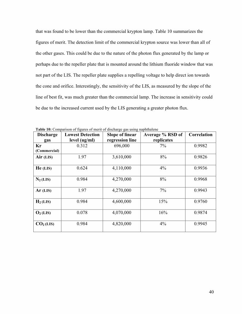
that was found to be lower than the commercial krypton lamp. Table 10 summarizes the

figures of merit. The detection limit of the commercial krypton source was lower than all of

the other gases. This could be due to the nature of the photon flux generated by the lamp or

perhaps due to the repeller plate that is mounted around the lithium fluoride window that was

not part of the LIS. The repeller plate supplies a repelling voltage to help direct ion towards

the cone and orifice. Interestingly, the sensitivity of the LIS, as measured by the slope of the

line of best fit, was much greater than the commercial lamp. The increase in sensitivity could

be due to the increased current used by the LIS generating a greater photon flux.

Table 10: Comparison of figures of merit of discharge gas using naphthalene Discharge

gas Lowest Detection

level (ug/ml) Slope of linear regression line

Average % RSD of replicates

Correlation

Kr (Commercial)

0.312 696,000 7% 0.9982

Air (LIS) 1.97 3,610,000 8% 0.9826

He (LIS) 0.624 4,110,000 4% 0.9936

N2 (LIS) 0.984 4,270,000 8% 0.9968

Ar (LIS) 1.97 4,270,000 7% 0.9943

H2 (LIS) 0.984 4,600,000 15% 0.9760

O2 (LIS) 0.078 4,070,000 16% 0.9874

CO2 (LIS) 0.984 4,820,000 4% 0.9945

41

3.1.3.1 Krypton discharge lamp

The results of the evaluation of the commercial krypton discharge lamp is given in Table 11.

The commercial krypton discharge lamp had a limit of quantification less than 0.312 ug/ml.

Peak area response was found to be linear from 0.312 ug/ml to 73.9 ug/ml with a correlation

coefficient of 0.9982. The average percent relative standard deviation was 7% between the

three replicate samples. The linear relation is defined by peak area = (696,000+/- 6,000) x

[Naph Conc.] - (500,000 +/- 300,000). An analytical calibration curve of peak area to

concentration is given in Figure 6. The residual analysis in Figure 7 supports the linear

relation between concentration and peak area for the commercial lamp.

Table 11: Peak area as a function of naphthalene concentration [Naphthalene]

(ug/ml)

Peak Area % RSD

1 2 3

0.312 210,913 178,415 181,409 9

0.624 531,333 550,500 499,568 14

0.984 505,403 568,689 534,133 6

1.97 1,287,752 1,109,774 1,152,917 10

3.94 2,433,902 2,514,515 2,476,247 2

24.6 16,831,232 17,359,430 17,323,798 3

49.3 32,306,436 35,131,560 33,661,750 4

73.9 50,632,636 49,299,932 51,106,128 4

42

Calibration Curve of Krypton Discharge Lamp to Naphthalene Concentration

0 20 40 60 800

2×1007

4×1007

6×1007

Concentration (ug/ml)

Pea

k A

rea

Figure 6: Analytical calibration curve of naphthalene to krypton discharge

Residuals of Krypton Linear Model Fitting

0 20 40 60 80-4×10+05

-2×10+05

0

2×1005

4×1005

6×1005

Dis

tanc

e fro

m L

inea

r lin

e

Naphthalene Concentration (ug/ml)

Figure 7: Residuals of naphthalene linear regression for krypton discharge

43

3.1.3.2 Air discharge lamp

The results of the evaluation of the air discharge lamp is given in Table 12. The air discharge

lamp had a limit of quantification less than 1.97 ug/ml. Peak area response was found to be

linear from 1.97 ug/ml to 73.9 ug/ml with a correlation coefficient of 0.9826. The average

percent relative standard deviation was 8% between the three replicate samples. The linear

relation is defined by Peak Area = (3,610,000+/- 70,000) x [Naph Conc.] - (3,000,000 +/-

3,000,0000). An analytical calibration curve of peak area to concentration is given in Figure

8. The residual analysis in Figure 9 supports the linear relation between concentration and

peak area for the air discharge LIS.


(ug/ml)

Peak Area % RSD

1 2 3

1.97 2,012,329 1,502,758 1,934,591 15

3.94 9,437,088 8,665,399 9,935,793 7

24.6 90,926,720 81,302,960 87,712,119 6

49.3 170,877,681 189,410,278 181,726,138 5

73.9 265,131,856 243,721,136 267,737,025 5

44

Figure 8: Analytical calibration curve of naphthalene to air discharge

Residuals of Air Discharge Linear Model Fitting

0 20 40 60 80-5×10+06

0

5×1006

1×1007

Dis

tanc

e fro

m L

inea

r lin

e


Figure 9: Residuals of naphthalene linear regression for air discharge

45

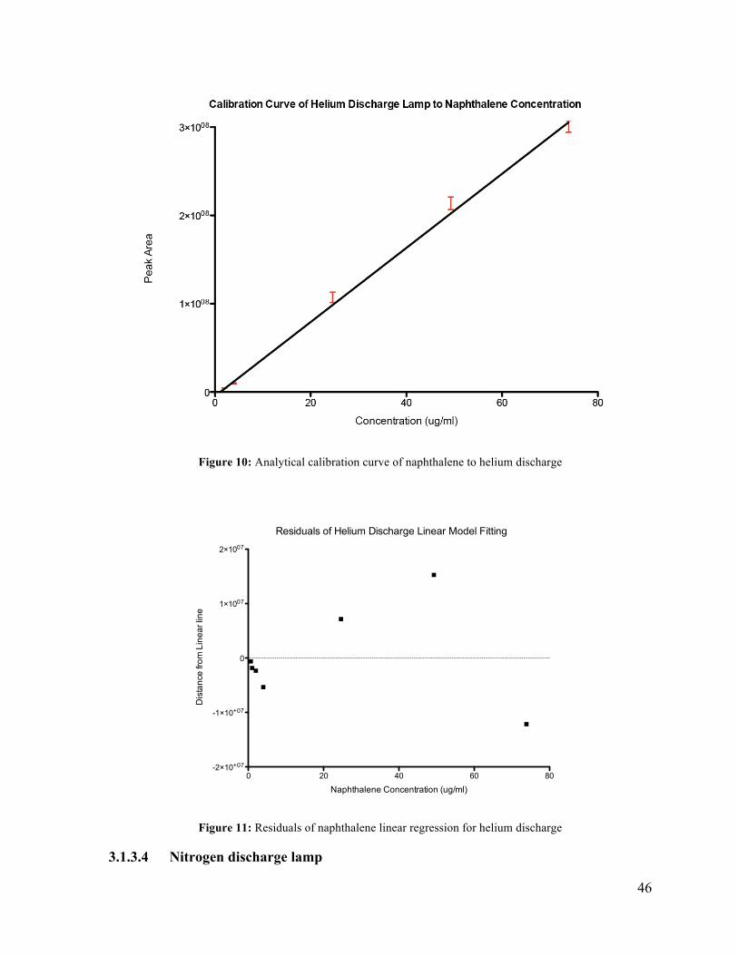
3.1.3.3 Helium discharge lamp

The results of the evaluation of the helium discharge lamp is given in Table 13. The helium

discharge lamp had a limit of quantification less than 0.624 ug/ml. Peak area response was

found to be linear from 0.624 ug/ml to 73.9 ug/ml with a correlation coefficient of 0.9936.

The average percent relative standard deviation was 4% between the three replicate samples.

The linear relation is defined by peak area = (4,110,000+/- 80,000) x [Naph Conc.] -

(1,000,000 +/- 3,000,0000). An analytical calibration curve of peak area to concentration is

given in Figure 10. The pattern of the residual analysis in Figure 11 indicates a non-linear

relation between concentration and peak area for the helium LIS.


(ug/ml)

Peak Area % RSD

1 2 3

0.624 773,995 743,697 800,806 4

0.984 1,046,226 1,028,982 1,042,337 0.9

1.97 4,417,981 4,620,392 4,726,839 3

3.94 10,351,792 9,079,291 9,627,322 7

24.6 100,527,144 108,993,472 111,952,704 6

49.3 209,137,312 218,302,480 223,180,860 3

73.9 297,153,856 283,781,848 291,109,332 2

46

Figure 10: Analytical calibration curve of naphthalene to helium discharge

Residuals of Helium Discharge Linear Model Fitting

0 20 40 60 80-2×10+07

-1×10+07

0

1×1007

2×1007

Dis

tanc

e fro

m L

inea

r lin

e


Figure 11: Residuals of naphthalene linear regression for helium discharge

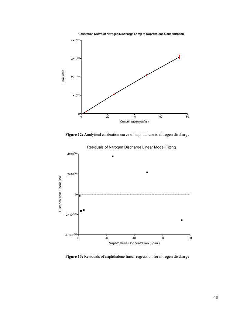
3.1.3.4 Nitrogen discharge lamp

47

The results of the evaluation of the nitrogen discharge lamp is given in Table 14. The

nitrogen discharge lamp had a limit of quantification less than 0.984 ug/ml. Peak area

response was found to be linear from 0.984 ug/ml to 73.9 ug/ml with a correlation coefficient

of 0.9968. The average percent relative standard deviation was 8% between the three

replicate samples. The linear relation is defined by peak area = (4,270,000+/- 60,000) x

[Naph Conc.] - (3,000,000 +/- 2,000,0000). An analytical calibration curve of peak area to

concentration is given in Figure 12. The pattern of the residual analysis in Figure 13 indicates

a linear relation between concentration and peak area for the nitrogen LIS.


(ug/ml)

Peak Area % RSD

1 2 3

0.984 985,843 893,877 994,875 5

1.97 3,722,166 3,132,420 4,144,695 13

3.94 11,431,726 10,126,985 14,860,112 20

24.6 105,641,744 104,100,336 106,982,928 1

49.3 209,400,336 203,828,032 214,765,952 3

73.9 300,437,888 298,034,221 330,085,376 2

48

Calibration Curve of Nitrogen Discharge Lamp to Naphthalene Concentration

0 20 40 60 800

1×1008

2×1008

3×1008

4×1008

Concentration (ug/ml)

Pea

k A

rea

Figure 12: Analytical calibration curve of naphthalene to nitrogen discharge

Residuals of Nitrogen Discharge Linear Model Fitting

0 20 40 60 80-4×10+06

-2×10+06

0

2×1006

4×1006

Dis

tanc

e fro

m L

inea

r lin

e


Figure 13: Residuals of naphthalene linear regression for nitrogen discharge

49

3.1.3.5 Argon discharge lamp

The results of the evaluation of the argon discharge lamp is given in Table 15. The argon

discharge lamp had a limit of quantification less than 1.97 ug/ml. Peak area response was

found to be linear from 1.97 ug/ml to 73.9 ug/ml with a correlation coefficient of 0.9943. The

average percent relative standard deviation was 7% between the three replicate samples. The

linear relation is defined by peak area = (4,270,000+/- 60,000) x [Naph Conc.] - (3,000,000

+/- 2,000,0000). An analytical calibration curve of peak area to concentration is given in

Figure 14. The pattern of the residual analysis in Figure 15 indicates a linear relationship

between concentration and peak area for the argon LIS.


(ug/ml)

Peak Area % RSD

1 2 3

1.97 4,185,297 3,962,193 4,488,663 12

3.94 9,905,008 9,379,972 11,373,342 7

24.6 107,403,856 102,647,146 128,987,615 6

49.3 211,688,864 207,085,572 216,286,337 5

73.9 302,850,784 298,511,651 309,877,280 5

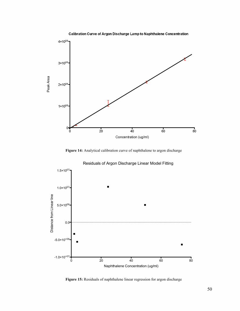
50

Figure 14: Analytical calibration curve of naphthalene to argon discharge

Residuals of Argon Discharge Linear Model Fitting

0 20 40 60 80-1.0×10+07

-5.0×10+06

0.0

5.0×1006

1.0×1007

1.5×1007

Dis

tanc

e fro

m L

inea

r lin

e


Figure 15: Residuals of naphthalene linear regression for argon discharge

51

3.1.3.6 Hydrogen discharge lamp

The results of the evaluation of the hydrogen discharge lamp is given in Table 16. The

hydrogen discharge lamp had a limit of quantification less than 0.984 ug/ml. Peak area


of 0.9760. The average percent relative standard deviation was 15% between the three

replicate samples. The linear relation is defined by Peak Area = (4,600,000+/- 200,000) x



a non-linear relationship between concentration and peak area for the hydrogen LIS.


(ug/ml)

Peak Area % RSD

1 2 3

0.984 1,294,011 1,588,879 1,077,721 20

1.97 4,190,329 4,898,725 3,917,152 12

3.94 10,651,292 8,044,139 12,998,573 23

24.6 111,462,552 115,996,350 96,599,609 9

49.3 211,413,136 248,299,176 260,890,731 11

73.9 321,106,176 369,864,798 279,838,803 14

52

Figure 16: Analytical calibration curve of naphthalene to hydrogen discharge

Residuals of Hydrogen Discharge Linear Model Fitting

0 20 40 60 80-2×10+07

-1×10+07

0

1×1007

2×1007

Dis

tanc

e fro

m L

inea

r lin

e


Figure 17: Residuals of naphthalene linear regression for hydrogen discharge

53

3.1.3.7 Oxygen discharge lamp

The results of the evaluation of the oxygen discharge lamp is given in Table 17. The oxygen

discharge lamp had a limit of detection of than 0.078 ug/ml. Peak area response was found to

be linear from 0.078 ug/ml to 73.9 ug/ml with a correlation coefficient of 0.9874. The

average percent relative standard deviation was 16% between the three replicate samples.

The linear relation is defined by Peak Area = (4,070,000+/- 90,000) x [Naph Conc.] -

(3,000,000 +/- 4,000,0000). An analytical calibration curve of peak area to concentration is

given in Figure 18. The pattern of the residual analysis in Figure 19 indicates a linear relation

between concentration and peak area for the oxygen LIS.


(ug/ml)

Peak Area % RSD

1 2 3

0.078 2,166,076 2,493,158 3,287,354 22

0.312 2,010,525 3,076,212 1,978,975 27

0.624 6,328,167 4,537,748 6,692,546 20

0.984 5,379,069 3,626,104 4,568,295 20

1.97 10,329,992 8,648,095 12,626,939 19

3.94 19,809,290 16,061,527 16,179,740 12

24.6 111,199,744 93,612,792 104,660,492 9

49.3 211,424,960 225,891,509 235,898,741 5

73.9 319,114,336 271,859,063 278,698,962 8

54

Figure 18: Analytical calibration curve of naphthalene to oxygen discharge

Residuals of Oxygen Discharge Linear Model Fitting

0 20 40 60 80-2×10+07

-1×10+07

0

1×1007

2×1007

3×1007

Dis

tanc

e fro

m L

inea

r lin

e


Figure 19: Residuals of naphthalene linear regression for oxygen discharge

55

3.1.3.8 Carbon dioxide discharge

The results of the evaluation of the carbon dioxide discharge lamp is given in Table 18. The

carbon dioxide discharge lamp had a limit of detection of than 0.984 ug/ml. Peak area


of 0.9945. The average percent relative standard deviation was 4.% between the three

replicate samples. The linear relation is defined by peak area = (4,820,000+/- 90,000) x



a linear relationship between concentration and peak area for the carbon dioxide LIS.


(ug/ml)

Peak Area % RSD

1 2 3

0.984 2,235,773 2,507,775 2,391,563 6

1.97 4,499,013 4,189,324 4,800,857 7

3.94 9,641,703 9,394,246 9,576,424 1

24.6 109,523,488 104,724,978 113,968,737 4

49.3 217,702,016 214,782,589 218,561,117 1

73.9 336,920,448 361,240,314 376,224,071 6

56

Figure 20: Analytical calibration curve of naphthalene to carbon dioxide discharge

Residuals of Carbon Dioxide Discharge Linear Model Fitting

0 20 40 60 80-1.5×10+07

-1.0×10+07

-5.0×10+06

0.0

5.0×1006

1.0×1007

Dis

tanc

e fro

m L

inea

r lin

e


Figure 21: Residuals of naphthalene linear regression for carbon dioxide discharge

57

3.1.3.9 Analysis of variance

ANOVA was used to determine whether the naphthalene calibration curves from each of the

gases were statistically different from one another. Generally, at lower concentrations the

differing gases were non-discernable from one another. At higher concentrations of

naphthalene differences were found to be significantly different between some gases. The

commercial krypton lamp was found to be the most significantly different from the other

LIS’s. Generally, the commercial lamp had a lower limit of detection than the LIS sources,

with the exception of oxygen. The correlation coefficient of the commercial lamp indicated a

stronger linear relation between detector response and analyte concentration.

The response of an air discharge was significantly similar to nitrogen. This was expected as

air contains a large majority of nitrogen and the emission spectra were similar. An

unexpected result was seen comparing air and oxygen and air and helium. A significant

difference in detector response was seen at 49.3 ug/ml but not at the concentrations above or

below 49.3 ug/ml. This is a peculiar result that could be resolved with a larger number of

replicates.

58

The lowest detected concentration was the same for both the air discharge and the nitrogen

discharge. However, the sensitivity of the naphthalene to the air discharge was less than the

nitrogen discharge. It is possible components, other than nitrogen, absorbed some of the

photons leading to a less efficient ionization efficiency.

An analysis of variance of the peak area measurements was done at each concentration to

determine whether the differences in measurements could be attributed to gas type or random

variation. The results of the analysis is given in Table 19. Comparisons were made between

peak areas for each gas at the eight concentration levels. In the case that no measurement was

recorded a “-“ signifies that no comparison was made. Gases that had no discernable (p >

0.05) differences are denoted “ns” and gases that had discernable differences are denoted “s”.

Table 19: ANOVA of response to concentration Kr O2 He N2 H2 CO2 Air Ar

Kr - ns, ns,

ns, ns,

ns, s, s,

s

-, ns,

ns, ns,

ns, s, s

-, -, ns.

ns, ns,

s, s, s

-, -, ns,

ns, ns,

s, s, s

-, -, ns,

ns, ns,

s, s, s

-, -, -,

ns, ns,

s, s, s

-, -, -,

ns, ns,

s, s, s

O2 - - -, ns,

ns, ns,

ns, ns,

ns, ns

-, ns,

ns, ns,

ns, ns,

ns, ns

-, -, ns,

ns, ns,

ns, ns, s

-, -, ns,

ns, ns,

ns, ns, s

-, -, -,

ns, ns,

ns, s, ns

-, -, -,

ns, ns,

ns, ns,

ns

He - - - -, -, ns, -, -, ns, -, -, ns, -, -, -, -, -, -,

59

ns, ns,

ns, ns,

ns

ns, ns,

ns, ns,

ns

ns, ns,

ns, ns, s

ns, ns,

ns, s, ns

ns, ns,

ns, ns,

ns

N2 - - - - -, -, ns,

ns, ns,

ns, ns,

ns

-, -, ns,

ns, ns,

ns, ns, s

-, -, -,

ns, ns,

ns, ns, s

-, -, -,

ns, ns,

ns, ns,

ns

H2 - - - - - -, -, ns,

ns, ns,

ns, ns, s

-, -, -,

ns, ns,

ns, s, s

-, -, -,

ns, ns,

ns, ns,

ns

CO2 - - - - - - -, -, -,

ns, ns,

ns, s, s

-, -, -,

ns, ns,

ns, ns,

s

Air - - - - - - - -, -, -,

ns, ns,

ns, ns,

s

60

3.2 Thermally Assisted Vapour Introduction

3.2.1 TAVI mass spectra

In positive mode, the mass spectra of mode naphthalene, biphenyl, anthracene, phenanthrene,

pyrene, fluoroanthrene, trans stilbene, rescorinol, salicylic acid, benzdiamine, ethyl-4-

aminobenzoate all exhibited strong M+ ion. Various novel organometallic compounds were

found to be amenable with TAVI producing molecular ions. Figure 22 shows the mass

spectrum of ferrocene. Ferrocene was found to have a high vapour pressure relative to the

other compounds tested and only required temperatures of around 80°C before strong,

dominant molecular peak was seen.

Figure 22: TAVI ms of Ferrocene

61

Structural information could be rationalized with TAVI APPI CID MS/MS. While high

energy electron impact ionization is distinct from collision induced dissociation,

fragmentation in both cases fragmentation is believed to be the result of internal energy

distribution resulting in fragmentation. Comparisons between EI spectra and CID MS/MS

showed general agreement to reference EI spectra. A compound with one of the strongest

signals was ferrocene (molecular weight 186.04 amu) with an impressively strong molecular

ion at m/z 186. CID on the molecular ion gave nearly identical mass spectra when compared

to reference EI spectra. The parent ion could be fragmented to reveal loss of a ring group

leaving and ion of m/z 121 easily identifiable as loss of a cyclopentadienyl ring seen in

Figure 23.

Figure 23: CID ms/ms Spectra of Ferrocene

62

The TAVI mass spectra of naphthalene is also dominated with molecular cation as shown in

Figure 24.

Figure 24: TAVI mass spectra of naphthalene

63

Figure 25 shows the TAVI mass spectra for biphenyl is dominated with the molecular ion.

Figure 25: TAVI ms of biphenyl

64

Cr(acac)3 had a strong molecular ion peak and when subjected to CID; readily produced

expected daughter ions that corresponded to electron impact shown in Figure 27.

Figure 26: TAVI ms of Cr(acac)3

65

Figure 27: TAVI ms/ms of Cr(acac)3

Not all compounds gave solely molecular ion peaks, Fe(acac)3 for example had a very strong

peak assigned as [M+H-acac]+ ([M - acac]+ peaks were seen by Hughes et al.) and also

Fe(acac)3 produced an ion assigned as [2M-acac]+. A crude sample of Cr(acac)3 exhibited

mostly molecular peak as shown in Figure 26. With moderate collision energy one of the

acac groups could be fragmented off leaving [M-acac]+. Under more powerful CID

conditions two acac groups could be removed. This selective fragmentation was useful in

determining the identity of the components of the analyte.

66

To further validate the usefulness of the technique some novel synthetic compounds were

tested. The crystal product of a synthesis, denoted as LG 113 (molecular weight 353.32 amu)

(C19H13F2N3O2) was found to have molecular cation of the desired product. Some of the

other peaks revealed unused starting product and possible unwanted by products shown in

figures 28 and 29. A reagent, fluorinated aniline, is easily seen in the TAVI mass spectrum at

111 amu in Figure 29.

Figure 28: TAVI ms of LG113

67

Figure 29: TAVI spectrum of LG113

68

In addition to identifying LG113, LG 159 with a molecular weight of 316.35 amu and a formula of

C20H16N2O2 was ionized by TAVI as shown in Figure 30 with a [M+H]+ peak.

Figure 30: TAVI spectra of LG159

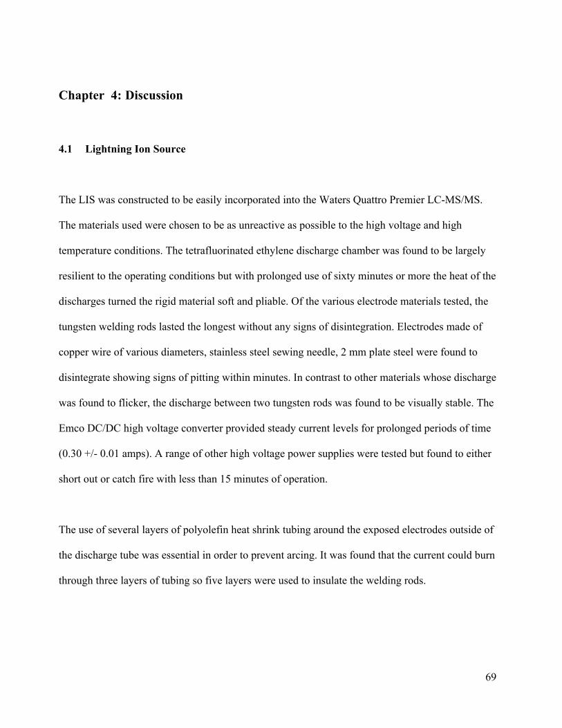
69

Chapter 4: Discussion


The LIS was constructed to be easily incorporated into the Waters Quattro Premier LC-MS/MS.

The materials used were chosen to be as unreactive as possible to the high voltage and high

temperature conditions. The tetrafluorinated ethylene discharge chamber was found to be largely

resilient to the operating conditions but with prolonged use of sixty minutes or more the heat of the

discharges turned the rigid material soft and pliable. Of the various electrode materials tested, the

tungsten welding rods lasted the longest without any signs of disintegration. Electrodes made of

copper wire of various diameters, stainless steel sewing needle, 2 mm plate steel were found to

disintegrate showing signs of pitting within minutes. In contrast to other materials whose discharge

was found to flicker, the discharge between two tungsten rods was found to be visually stable. The

Emco DC/DC high voltage converter provided steady current levels for prolonged periods of time

(0.30 +/- 0.01 amps). A range of other high voltage power supplies were tested but found to either

short out or catch fire with less than 15 minutes of operation.

The use of several layers of polyolefin heat shrink tubing around the exposed electrodes outside of

the discharge tube was essential in order to prevent arcing. It was found that the current could burn

through three layers of tubing so five layers were used to insulate the welding rods.

70

4.1.1 Emission spectra

Many of the emission lines listed in the NIST reference spectra were found in the experimental

results for each gas in the 200 to 960 nm range. A reference emission line was considered to have

matched an experimental peak if the reference point fell within the range of a measured emission

peak. Even though photons of wavelengths less than 200 nm could not be measured with the

spectrometer it has previously been shown that high energy photons are produced from electrical

discharges (Lyman, 1906; Hopfield, 1930; Tanaka et al., 1958) but given the optical properties of

the lithium fluoride window it can be assumed that no photons with wavelength less than 105 nm

made it out of the discharge chamber and be available for ionization. This does leave any photons

of wavelength longer than 105 nm available for ionization.

Argon and nitrogen had the largest number of emission lines that matched as shown in figures 4

and 5. While the relative intensities of the measured lines did not match up to the reference spectra

differences in discharge gas pressure and electrode distance have been found to produce different

peak shapes and intensities (Lalos and Hammond, 1961; Abdel-Fattah, E., et al., 2011; Namba, S.,

et al., 2011). The LIS operates at approximately 1 atmosphere.

The emission profile of pure nitrogen discharge was found to have many shared emission peaks

compared to the spectra of the air based discharge. Since the majority of air is nitrogen, this opens

the possibility of using readily available air instead of nitrogen as a discharge gas.

71

4.1.2 Mass spectra

The LIS apparatus produced molecular ions. A representative polycyclic aromatic hydrocarbon,

pyrene, produced primarily strong molecular ion or pseudo molecular ion ([M+H]+) in both the lab

and commercial source. The results of the LIS are in general agreement with other photon based

ionization methods (Syage, J., 2004; Kersten, H., et al., 2009). Slight differences in the ratio of

M+/[M+H]+ and [M+2H]+ were found between the LIS and the commercial krypton lamp. While

efforts were taken to match as many of the ion source parameters in an attempt to match the ion

source energetics, perhaps the lack of a repeller plate on the LIS is responsible for the differences.

It is noteworthy that the LIS produced a two-fold stronger response compared to the commercial

APPI krypton discharge source. 17-α-hydroxyprogesterone produced similar [M+H]+ spectra in

the two techniques with the lab built source having a higher response factor. The increased signals

from the lab built source may be due to a higher discharge current and possibly a more transparent

lithium fluoride window (Gerasimova, N., 2006).

4.1.3 Calibration curve

In contrast to the recent atmospheric pressure photoionization literature (Robb et al., 2000), a

variety of gases were able to ionize anaytes with similar analytical figures of merit as a krypton

discharge lamp. A statistical analysis of the results found differences between the gases at higher

concentrations but at lower concentrations no significant differences were found.

72

4.2 Demonstrating APPI for characterization of synthetic products

Using a Waters Quattro Premier LC MS/MS fitted with a Syagen PhotoMate™ photoionization

lamp, samples of pure compounds and mixtures were heated using the TAVI device and the

vapours released were monitored by APPI MS. This effectively generated molecular ions for the

compounds tested. These spectra were easily generated within seconds. In addition to this,

collision induced dissociation spectra were collected from some of these molecular ions. As it is

demonstrated above, structural information and limited functional group analysis can be done

using TAVI CID. Previously, vapours of pure aromatic compounds were photoionized in an effort

to determine the mechanism of the formation of [M+H]+ often seen in photoionization spectra

(Syage, J., 2004) but this appears to be the first report of photoionizing vapours of organometallic

compounds for structure determination. Similar techniques of ionizing analyte vapours have used

other ionization methods like corona discharge in the case of Atmospheric Solids Analysis Probe

(McEwen et al., 2009).

The impetus of this research grew from requests from a synthetic chemist who required

confirmation of their synthetic reactions. Compound solubility and small sample size where two

challenges presented. TAVI does not require a liquid sample solution and could easily determine

the molecular weights of insoluble organometallic crystals with minimal sample preparation. Solid

samples were tapped into a glass melting point capillary tube which was resistively heated directly

below the photoionization lamp. Liquid samples could be either injected in a heated glass capillary

tube or spotted onto a lithium fluoride plate that was held directly in front of the photoionization

lamp. TAVI APPI MS/MS offers simple mass spectra dominated by molecular ion, M+, signals

compared to solvent based APPI which generally leads to [M+H]+. To demonstrate the

73

effectiveness of TAVI APPI MS/MS, a range of PAH and organometallic compounds were

examined. For the majority of compounds molecular ions were observed as demonstrated by

spectra of naphthalene, pyrene and ferrocene.

In addition to molecular weight information, collision induced dissociation offered information

about the structure on the compounds. For example, ferrocene could be fragmented to lose one of

the five membered rings. Cr(acac)3 could be selectively fragmented to lose one or two of the acac

groups yielding structural information.

There have been various recent attempts to find an appropriate mass spectrometric techniques to

analyze organometallic and coordination compounds. Previous work by Dorcier et al. using

photoionization on organometallic compounds dissolved in solvents produced mixed results;

molecular ions were observed but significant toluene substitution, analyte methylation and various

unidentified peaks were also observed (Dorcier et al., 2006). A “solvent-free” technique is

desirable for insoluble compounds or compounds that may dissociate in solution. The technique

described here meets that objective. A recent paper by Hughes et al. reported success with the use

of MALDI-TOFMS on organometallic and coordination compounds (Hughes et al., 2009). For

most of the compounds evaluated, strong molecular ions were observed, but sodium and potassium

adducts were also observed. As demonstrated by Syage, 2004, vapours examined by APPI

generate molecular ions (M+)

Carrying on from this preliminary work, several aspects of the thermally assisted vapour

introduction technique could be refined to allow for analysis of air sensitive compounds and

74

quantitative measurements. The suitability of sequential thermal desorption could be investigated

for multicomponent samples.

75

Chapter 5: Conclusions

5.1 Summary

The overall goal of this thesis was to examine the validity of two separate hypothesis both dealing

with atmospheric pressure photoionization: To determine whether a variety of common gases

could be used as discharge gases for ionization; and whether photoionization of vapours generated

from solid samples could allow molecular weight determination and some structural information.


The inexpensive Lightning Ion Source has shown that it can be used to identify molecular masses

and determine some functional groups in test compounds. The results of the three sets of analysis;

photon emission profile, mass spectra with M+ and [M+H]+ and comparable analytical response to

the commercial lamp, demonstrate its usefulness.

Using the custom fabricated LIS it was found that photons produced from an electrical discharge

in all of the gases tested could photoionize a variety of test compounds. The LIS was different

from commercial photoionization sources in two important ways. The LIS had a discharge at

atmospheric pressure whereas the two commercial sources are both contain low pressure discharge

chambers. Additionally, the LIS was found to be effective with a variety of discharge gases

whereas the commercial sources specifically use krypton as the discharge gas. Significant

differences were found between the response to the analytes depending on the discharge gas used.

The majority of the discharge gases used in the LIS had greater sensitivity but lower limit of

76

detection when compared to the krypton lamp. Additionally, the mass spectra generated by the LIS

did exhibit difference ratios of M+/[M+H]+/[M+2 amu]+ but in many ways the inexpensive LIS was

found to be a powerful tool comparable to the commercial source.

Carrying on from this preliminary work, several aspects of the LIS could be refined. For instance,

the effect on electrode distance and position has on photon flux and subsequent ionization could be

examined to maximize ionization. Related to electrode orientation, discharge current could be

examined to identify an optimum current for maximum ionization. Further testing to evaluate the

applicability of the source may be useful to produce an inexpensive ion source for use on any

atmospheric pressure ionization mass spectrometer.

Applications such as petrochemical analysis or screening for explosives in security applications

maybe useful, especially with the finding that common air can be used as a discharge gas giving

similar analytical results to commercial photoionization techniques. The US Transportation Safety

Administration is responsible for screening over 700 million passengers and support staff annually

at a cost of over one billion dollars (Elias, B., 2009). A key requirement is the screening of

explosives and drugs of abuse, two applications well suited to photoionization (Syage, J., 2006).

Most interesting, is the use of the LIS for remote or field analysis. With air being an effective

discharge gas, LIS may be useful in field analysis where operating supplies are hard to obtain.

77

5.3 Thermally Assisted Vapour Introduction

Using a custom configured heating apparatus to produce vapours of a range of test compounds

thermally assisted vapour introduction was found to offer rapid characterization without solvents.

In instances where samples are not soluble in common solvents or when limited sample size is an

issue TAVI may be an effective method to determine molecular weight and even determine some

functional group information quickly.

Carrying on from this preliminary work, several aspects of the thermally assisted vapour

introduction technique could be refined to allow for analysis of air sensitive compounds and

quantitative measurements. For air sensitive compounds analytes can be sealed within a melting

point tube and inserted into the TAVI apparatus. It is likely that the source block could be flooded

with an inert gas displacing the offending oxygen. The melting point tube could be heated and

broken to release the vapours into the inert environment of the source block where they could be

ionized by photons. Another avenue of future development could be to determine the suitability of

sequential thermal desorption that could be used for multicomponent samples.

78

References

Abdel-Fattah, E., Bazavan, M., Sugai, H., Langmuir probe diagnostics of electron energy

distributions with optical emission spectroscopy in capacitively coupled rf discharge in

nitrogen, J. Appl. Phys., 113303-8, 2011.

Al- Joboury, Turner, D., Molecular Photoelectron Spectroscopy. Part I The Hydrogen and

Nitrogen Molecules, 5141- 5147, 1963.

Andrade, F., Wetzel, W., Chan, G., Webb, M., Gamez, G., Ray, S., Hieftje, G., A New, Versatile,

Direct- Current Helium Atmospheric- Pressure Glow Discharge, J. Am. At. Spectrom., 21,

1175-1184, 2006.

Antonov, V., Letokhov, V., Shibanov, A. , Formation of Molecular Ions as a Result of Irradiation

of the Surface of Molecular Crystals by UV laser Radiation, 441-444, 1980.

Banning, M., The Far Ultraviolet Refectivities of Metallic Films, J. O. S. A., 32, 98-102, 1942.

Borsdorf, H., Nazarov, E., Miller, R., Time-of-Flight Ion Mobility Spectrometry and Differential

Mobility Spectrometry; A Comparative study of their efficiency in the analysis of

halogenated compounds, Talanta, 71, 1804-1812, 2007.

Bos, B., van Leeuwan, S., Karst, U., From Fundamentals to Applications: Recent Developments in

Atmospheric Pressure Photoionization Mass Spectrometry, Anal. Bioanal. Chem., 384, 85-

99, 2006.

Brion, C., An Improved Mass Spectrometer Photoionization Source, Analytical Chemistry, 38,

1941-1942, 1966.

Clark, I., Frost, D., A Study of the Energy Levels in Benzene and some Fluorobenzenes by

Photoelectron Spectroscopy, J. Am. Chem. Soc, 89, 244-247, 1966.

Cody, R., Laramée, J., Durst, H., Versatile New Ion Source for the Analysis of Materials in Open

79

Air Under Ambient Conditions, Anal. Chem, 77, 2297-2302, 2005.

Ditchburn, R., Arnot, F., The Ionisation of Potassium Vapour, Proc Royal Soc, 516- 536, 1929.

Dorcier, A., Dyson, P., McIndoe, J., Analysis of Coordination and Organometallic Compounds

using Photoionization Mass Spectrometric Techniques, Eur. J. Inorg. Chem, 4294-4297,

2003.

Driscoll, J., Photoionization Monitor for Oxides of Nitrogen, US Patent 40,359/72, 1972.

Driscoll, J., Warneck, P. , The Analysis of PPM Levels of Gases in Air by Photoionization Mass

Spectrometry, Journal of the Air Pollution Control Association, 23, 858- 863, 1973.

Druyvesteyn, M., Penning, F., The Mechanism of Electrical Discharges in Gases of Low Pressure,

Reviews of Modern Physics, 12, 87- 175, 1940.

Duncanson, A., Stevenson, W., Some Properties of Magnesium Fluoride Crystallized from the

Melt, 1001-1006, 1958.

Eelman, M., Blacquiere, J., Moriarty, M., Fogg, D., et al., Shining New Light on an Old Problem:

Retooling MALDI Mass Spectrometry for Organotransition-Metal Catalysis, Chem. Int. Ed.,

303-306, 2008.

Einstein, A., On a Heuristic Point of View about the Creation and Conversion of Light. Translated

by Haar, D.

Elias, B., Airport Passenger Screening: Background and Issues for Congress, Congressional

Research Service, 2009.

Frost, D., McDowell, C., Vroom, D., Photoelectron Kinetic energy Analysis in Gases by means of

Spherical Analyser, Proceedings of the Royal Society of London. Series A, Mathematical

and Physical Sciences, 296, 566-579 , 1967.

Gerasimova, N., CaF2, MgF2, SiO2, Al2O3, SiC, LiF, BaF2, and ZrO2 Optical Single Crystals

80

used in Studies in the VUV Spectral Region, Instruments and Experimental Techniques, 49,

408-412, 2006.

Gurley, N. Beloukhina, K. Boudreau, A. Klegeris, W. S. McNeil, The Synthesis and

Characterization of a Series of Cobalt(II) β-Ketoaminato Complexes and Their Cytotoxic

Activity Towards Human Tumor Cell Lines, J. Inorg. Biochem., 105, 858-866, 2011.

Gross, M., Caprioli, R., The Encyclopedia of Mass Spectrometry, Elsevier, Vol 6, 2007.

Gyulai, Z., Die Dispersion Einiger Alkalihalogenide im Ultravioletten, 80-87, 1927.

Haapala, M., Pól, J., Saarela, V., Kotiaho, T., Ketola, R., Franssila, S., Kauppila, T., Kostainen, R.,

Desorption Atmospheric Pressure Photoionization, Anal. Chem, 79, 7867- 7872, 2007.

Harper, J., Charipar, N., Mulligan, C., Zhang., X., Cooks, G., Ouyang., Low-Temperature Plasma

Probe for Ambient Desorption Ionization, Anal. Chem., 9097-9104, 2008.

Hass, G., Tousey, R., Reflective Coatings for the Extreme Ultraviolet, J. Opt. Soc Am., 49, 593-

602, 1959.

Herzog, R., Marmo, F., Mass Spectroscopic Determination of Photoionization Products, The

Journal of Chemical Physics, 27, 1202-1205, 1957.

Hopfield, J., Absorption and Emission Spectra in the Region l600-1100, Phys. Rev, 1133-1134,

1930.

Hopfield, J., New Ultra-violet Spectrum of Helium, The Astrophysical Journal, 72, 133-150, 1930.

Huffman, R., Larrabee, J., Tanaka, Y., Rare Gas Continuum Light Sources for Photoelectric

Scanning in the Vacuum Ultraviolet, Applied Optics, 4, 1581-1588, 1965.

Hughes, L., Wyatt, M., Stein, B., Brenton, A., Investigation of Solvent-Free MALDI-TOFMS

Sample Preparation Methods for the Analysis of Organometallic and coordination

Compounds, Anal. Chem., 81, 543-550, 2009.

81

Jensen, C., Libby, W., Intense 584-Å, Light from a Simple Continuous Helium Plasma, 135, 1247-

1252, 1964.

Jones, E., Harrison, A., Asymmetric Charge Transfer Reactions of Rare Gas Ions at Low Ion

Energies, Int. J. Mass Spectrom. Ion Phys., 6, 77-88, 1971.

Kato, R., Optical Properties of LiF in the Extreme Ultraviolet, 2525-2533, 1961.

Kato, R., Nakashima, S., Optical Properties of Irradiated LiF Crystals in the Extreme Ultraviolet

Region, J. Phys. Soc. Japan, 15, 2111-2112, 1960.

Kauppila, T., Kuuranne, T., Meurer, E., Eberlin, M., Kotiaho, T., Kostiainen, R., Atmospheric

Pressure Photoionization Mass Spectrometry. Ionization Mechanisms and the Effect of

Solvent on the Ionization of Naphthalenes, Anal. Chem, 74, 5470-5479, 2002.

Kersten, H., Funcke, V., Lorenz, M., Brockmann, K., Benter, T., O'Brien, R., Evidence of Neutral

Radical Induced Analyte Ion Transformation in APPI, and Near-VUV APLI, J. Am. Chem.

Soc, 2009, 1868-1880, 2009.

Kinsinger, J., Stebbings, W., Valenzi, R., Taylor, J., Spectral Evaluation of a Sealed Helium

Discharge Lamp for Studies in Photoelectron Spectroscopy, Anal. Chem, 44, 773-777, 1972.

Kiser, R., Introduction to Mass Spectrometry and its Applications, Prentice-Hall Inc, 1965.

Lalos, G., Hammond, G., Emission Spectra of Hot Dense Gases, 616-627, 1961.

Lorenz, M., Schiewek, R., Brockman, K., Schmitz, O., Gäb, S., Benter, T., The Distribution of Ion

Acceptance in Atmospheric Pressure Ion Sources: Spatially Resolved APLI Measurements,

J. Am Soc Mass Spectrom, 19, 400-410, 2008.

Lossing, F., Tanaka, I., Photoionization as a Source of Ions for Mass Spectrometry, J. Chem.

Phys., 25, 1031-1034, 1956.

Lubben, A., McIndoe, J., Weller, A., Coupling an Electrospray Ionization Mass Spectrometer with

82

a Glovebox: A Straightforward, Powerful, and Convenient Combination for Analysis of Air-

Sensitive Organometallics, Organometallics, 3303-3306, 2008.

Lyman, T., The Spectrum of Hydrogen in the Region of Extremely Short Wave-length, The

Astrophysical Journal, 23, 181- 214, 1906.

Lyman, T., The Spectrum of Helium in the Extreme Ultra-violet, Science, 59, 422, 1924.

Lyman, T., The Spectrum of Helium in the Extreme Ultra-violet, Nature, 113, 785, 1924.

Lyman, T., The Spectrum of Helium in the Extreme Ultra-violet, The Astrophysical Journal, 60, 1-

15, 1924.

Lyman, T., On the Spectra of Neon and Argon in the Extreme Ultra-violet, Nature, 116, 358, 1925.

Lyman, T., Saunders, F., The Spectrum of Neon in the Extreme Ultra-violet. Proc. N. A. S., 12,

92-96, 1926.

Madden, R., Canfield, L., Apparatus for the Measurement of Vacuum Ultraviolet Optical

Properties of Freshly Evaporated Films, Journal of the Optical Society of America, 51, 838-

845, 1961.

McEwen, C., McKay, R., Larsen, B., Analysis of Solids, Liquids, and Biological Tissues Using

Solids Probe Introduction at Atmospheric Pressure on Commercial LC/MS Instruments,

2005, 7826-7831, 2005.

McEwen, C. and Larsen, B., Ionization Mechanisms Related to Negative Ion APPI, APCI, and

DART, J am Soc Mass Spectrom, 1518-1521, 2009.

Milgram, A., Givens, M., Extreme Ultraviolet Absorption by Lithium Fluoride, Phys. Rev, 125,

1506-1509, 1962.

Millikan, R., Bowen, I., Extreme Ultra-violet Spectra, The Physical Review, 23, 1-38, 1924.

Namba, S., Yamasaki, T., Hane, Y., Fukuhara, D., Kozue, K., Takiyama. K., Emission

83

spectroscopy of a microhollow cathode discharge plasma in helium-water gas mixtures, J.

Appl. Phys., 073307-5, 2011.

NIST Webbook (2009). Atomic Spectra Database. Retrieved from

http://www.nist.gov/pml/data/asd.cfm.

Nordling, C., Sokolowski, E., Siegbahn, K., Precision Method for Obtaining Absolute Values of

Atomic Binding Energies, Phys. Rev, 105, 1676-1677, 1957.

Patterson, D., Vaughan, W., Influence of Crystal Surface on the Optical Transmission of Lithium

Fluoride in the Vacuum- Ultraviolet Spectrum, J. Opt. Soc. Am., 53, 851-855, 1963.

Poschenrieder, W., Warneck, P., Gas Analysis by Photo-ionization Mass Spectrometry, Journal of

Applied Physics, 37, 2812-2820, 1966.

Poschenrieder, W., Warneck, P., Mass Spectrometric Gas Analysis Utilizing Selective Photo

ionization, , 40, 383-390, 1968.

Raffaelli, A., Saba, A., Atmospheric Pressure Photoionization Mass Spectrometry, Mass

Spectrometry Reviews, 22, 318-331, 2003.

Revel'skii, I., Yashin, Y., Mass Spectrometry with Photoionization at Atmospheric Pressure and

the Analysis of Multicomponent Mixtures Without Separation, Chemical and

Physicochemical Methods of Analysis, 243-248, 1991.

Robb, D., Bruins, A., Atmospheric Pressure Photoionization (APPI): A New Ionization Method

for Liquid Chromatography- Mass Spectrometry, US Patent 6,534,765 B1, 2003.

Robb, D., Covey, T., Bruins, A., Atmospheric Pressure Photoionization: An Ionization Method for

Liquid Chromatography - Mass Spectrometry, Anal. Chem, 72, 3653-3659, 2000.

Sabine, G., Reflectivities of Evaporated Metal Films in the Near and Far Ultraviolet, 55, 1064-

1069, 1939.

84

Schneider, E., Optical Properties of Lithium Fluoride in the Extreme Ultraviolet, The Physical

Review, 49, 341-345, 1936.

Sieck, L., Gorden, R., Photoionization of Simple Hydrocarbons at 73.6-74.4 and 58.4 nm.

Comparison with Penning Ionization, Chemical Physical Letters, 19, 509-512, 1973.

Syage, J., Real-Time Multispecies Monitoring by Photoionization Mass Spectrometry, US Patent

5,808,299, 1998.

Syage, J., Mechanism of [M+H]+ Formation in Photoionization Mass Spectrometry, J. Am Soc

Mass Spectro, 15, 1521-1533, 2004.

Syage, J., Evans, M., Hanold, K., Photoionization Mass Spectrometry, American Laboratory,

2000.

Syage, J., Hanning-Lee, M., Hanold, K., A Man-Portable, Photoionization Time-of-Flight Mass

Spectrometer, Field Analytical Chemistry and Technology, 204-215, 2000.

Syage, J., Hanold, K., Rapid Response Mass Spectrometer, US Patent 6,326,615 B1, 2001.

Syage, J., Hanold, K., Lynn, T., Horner, J, Atmospheric Pressure Photoionization II. Dual Source

Ionization, J. Chrom. A, 1050, 137-149, 2004.

Syage, J., Cai, S., Li, J., Evans, M., Direct Sampling of Chemical Weapons in Water by

Photoionization Mass Spectrometry, Anal. Chem., 78, 2967-2976, 2006.

Takáts, Z., Wiseman, J., Gologan, B., Cooks, R., Mass Spectrometry Sampling Under Ambient

Conditions with Desorption Electrospray Ionization, Science, 306, 471-473, 2004.

Tanaka, Y., Continuous Emission Spectra of Rare Gases in the Vacuum Ultraviolet Region, J. Opt.

Soc. Am., 45, 710- 713, 1955.

Tanaka, Y., Jursa, A., LeBlanc,F., Continuous Emission Spectra of Rare Gases in the Vacuum

Ultraviolet Region II Neon and Helium, Journal of the Optical Society of America, 48, 304-

85

308, 1958.

Venter, A., Nefliu, M., Cooks, G., Ambient Desorption Ionization Mass Spectrometry, Trends in

Analytical Chemistry, 27, 284-290, 2008.

Walker, W., Samson, J., Rustgi, O., Optical Properties of Al for hv between 10 and 26 eV, Journal

of the Optical Society of America, 48, 71, 1958.

Webb, J., Analytical Photoionization Mass Spectrometer with an Argon Gas Filter Between the

Light Source and Monochromator, US Patent 3,521,054, 1970.

Wilkinson, P., Tanaka, Y., New Xenon-Light Source for the Vacuum Ultraviolet, Journal of the

Optical Society of America, 45, 344-349, 1955.

Wood, R., Optical Properties of Homogeneous and Granular Films of Sodium and Potassium,

Philosophical Magazine, 38, 98- 112, 1919.

Yamakita, Y., Yamauchi, M., Ohno, K., Penning Ionization Electron Spectra of Pyrene, Chrysene,

and Coronene in Collision with Metastable He(2 3S) Atoms in the Gas Phase, Journal of

Chemical Physics, 130, 24306, 2009.

Yamane, M., Photoionization Detector for Gases and Vapours, US Patent 3,454,828, 1969.

EXAMINING THE ROLE OF DISCHARGE GAS AND …davincarter.com/Davin/M._Sc._files/Davin Carter, M. Sc.,...

Documents

Transcript of EXAMINING THE ROLE OF DISCHARGE GAS AND …davincarter.com/Davin/M._Sc._files/Davin Carter, M. Sc.,...