Exact Sampling of Jump-Di usion Processes Sampling of Jump-Di usion Processes 3 Jump-Di usion Fix a...

1

Exact Sampling of Jump-Diffusion Processes

Kay Giesecke and Dmitry Smelov

Management Science & Engineering

Stanford University

Kay Giesecke

Exact Sampling of Jump-Diffusion Processes 2

Jump-Diffusion Processes

• Ubiquitous in finance and economics

– Price models: equity, commodity, rates, energy, FX

– Default timing models (jump component)

• We develop a method for the exact sampling of a jump-diffusion

process with state-dependent drift, volatility, jump intensity, and

jump size

– Leads to unbiased simulation estimators of derivative prices,

risk measures, and other quantities

• The method extends an innovative acceptance/rejection scheme

developed by Beskos & Roberts (2005, AAP) and Chen (2009) for

diffusions

Kay Giesecke


Jump-Diffusion

• Fix a filtered probability space (Ω,F ,F,P)

• For suitable functions µ and σ, consider the SDE

dXt = µ(Xt)dt+ σ(Xt)dWt + dJt

where W is a standard Brownian motion and J is a jump process

Jt =∑n≤Nt

c(XT−n, Zn)

– N is a counting process with event times (Tn) and intensity

λt = Λ(Xt−) for a suitable function Λ

– (Zn) is a sequence of mark variables valued in E

– c : DX × E → DX determines the jump magnitudes

• J is self-exciting; dependence between jump sizes and frequency

Kay Giesecke


Jump-Diffusion

• For a suitable function f and a horizon T we wish to calculate

Ef(XT , (Jt)t≤T )

– Price of a derivative written on XT

– Price of a credit derivative written on J

• Alternative approaches

– Analytical solutions: rare; e.g. Merton and Kou models

– Semi-analytical transform approaches: AJDs, LQJDs, Levy

– PIDE approaches: fewer restrictions

– Monte Carlo simulation: perhaps the widest scope

Kay Giesecke


Discretizing the Jump-Diffusion

Standard approach to simulating X

• X is approximated on a discrete-time grid

– Euler or higher order scheme for diffusion component

– Thinning or time-scaling scheme for jump times Tn

• Simulation estimator is biased

– Magnitude of the bias? Confidence intervals?

– Convergence of scheme?

– Allocation of computational budget?

Kay Giesecke


Discretizing the Jump-Diffusion

Time-scaling for jumps: Tnd= inft :

∫ t0

Λ(Xs)ds ≥ E1 + · · ·+ En

0 2 4 6 8 100.4

0.6

0.8

1

1.2

1.4

1.6

1.8

2

Time

Inten

sity

0

0.5

1

1.5

2

2.5

3

3.5

4

4.5

Loss

0 2 4 6 8 10

0

1

2

3

4

5

6

7

Time

Comp

ensat

or

T1(ω) T2(ω) T3(ω) T4(ω) T5(ω) T6(ω)

S1(ω)

S2(ω)

S3(ω)

S4(ω)

S5(ω)

S6(ω)

Kay Giesecke


Exact Sampling

• We provide an exact sampling scheme for X that avoids

discretization entirely, and leads to unbiased simulation estimators

• First step: transform X into a unit-diffusion SDE

– Lamperti transform F (x) =∫ xX0

1σ(u)du

– Then Yt = F (Xt) solves

dYt = α(Yt)dt+ dWt + dJYt

where

α(y) =µ(F−1(y))σ(F−1(y))

− 12σ′(F−1(y))

JYt =∑n≤Nt

∆(YT−n , Zn)

for ∆(y, z) = F (F−1(y) + c(F−1(y), z))− y

Kay Giesecke


Exact Sampling

Assumptions

1. σ(x) is bounded away from 0

2. µ(x) and Λ(x) are continuously differentiable and σ(x) is twice

continuously differentiable.

3. Conditions on α(y) and c(x, z) guaranteeing that Y does not

reach the boundaries in finite time (known).

Kay Giesecke


Acceptance/Rejection Scheme

• The exact method uses an A/R scheme

• Suppose we want to sample from a density f(y) and there is

another density g(y) and a constant c > 0 such that

c · f(y)g(y)

≤ 1

• A/R scheme

1. Draw a sample Y from g

2. Draw a Bernoulli variable I with success probability c · f(Y )g(Y )

3. Accept Y as a sample from f if I = 1

Kay Giesecke


A/R for Continuous Y

Beskos & Roberts (2005, AAP)

• We wish to sample YT using the A/R scheme

• Under Novikov and additional boundedness conditions,

fYT (y)g(y)

∝ E[

exp(−∫ T

0

φ(Ws)ds) ∣∣∣WT = y

]=: H(y)

where φ = (α′ + α2)/2 and g(y) is a proposal density

• For the A/R step, note that H(y) = P(MT = 0 |WT = y) where

M is a doubly-stochastic Poisson process with intensity φ(Ws)

– The Bernoulli indicator I = 1 = MT = 0 can be generated

by sampling MT given WT = Y with Y drawn from g

– If φ(x) ≤ π, then this can be done by thinning a Poisson

process with intensity π (requires sampling from BB)

Kay Giesecke



Localization: Chen (2009)

Kay Giesecke



Generating the first piece of Y

• Target exit time ζ1 = inft ≥ 0 : |Yt − Y0| ≥ L for L > 0

• Proposal exit time τ = inft ≥ 0 : |Wt| ≥ L

• The LR between (ζ1, Y1 − Y0) and (τ,Wτ ) is proportional to

E[

exp(−∫ τ

0

φ(Y0 +Ws)ds) ∣∣∣ τ,Wτ

]• Because of the continuity assumptions, φ(Y0 +Ws) is bounded

and thinning can always be used in the acceptance test

– Need to sample from Brownian meander

• The density of τ is known and can be sampled from using the

method of Burq & Jones (2006)

Kay Giesecke


A/R for Jump-Diffusion YIntroducing jumps

Kay Giesecke


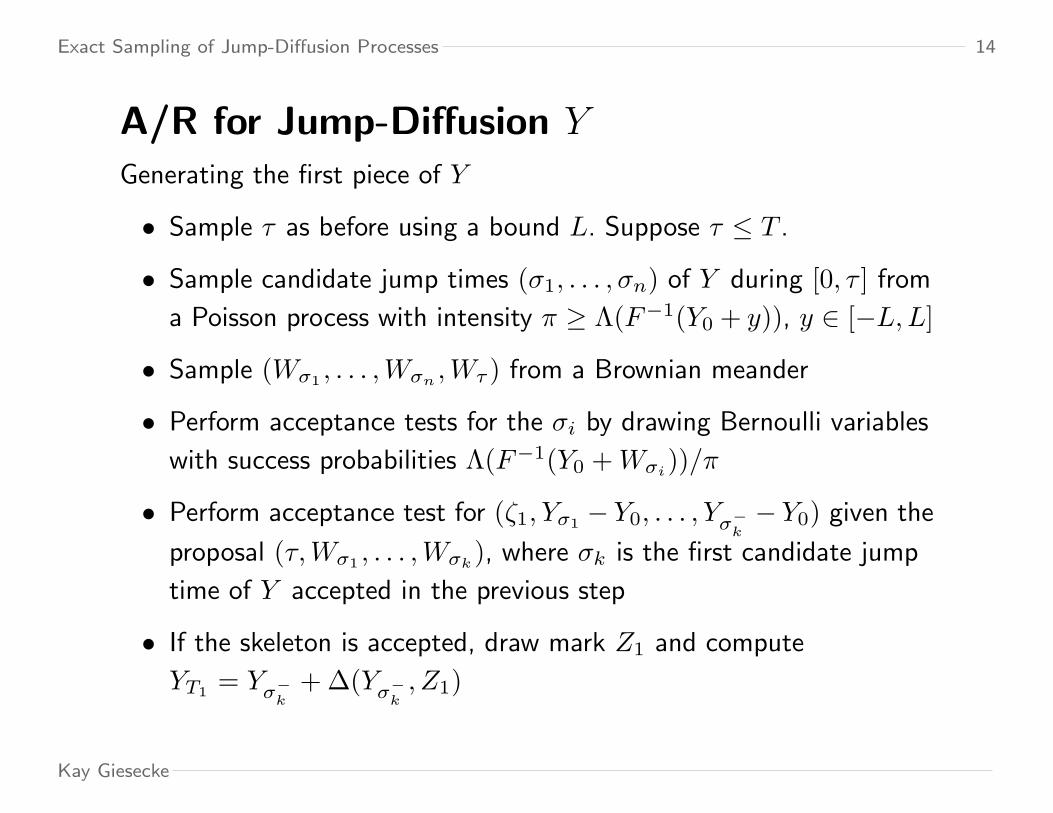
A/R for Jump-Diffusion YGenerating the first piece of Y

• Sample τ as before using a bound L. Suppose τ ≤ T .

• Sample candidate jump times (σ1, . . . , σn) of Y during [0, τ ] from

a Poisson process with intensity π ≥ Λ(F−1(Y0 + y)), y ∈ [−L,L]

• Sample (Wσ1 , . . . ,Wσn ,Wτ ) from a Brownian meander

• Perform acceptance tests for the σi by drawing Bernoulli variables

with success probabilities Λ(F−1(Y0 +Wσi))/π

• Perform acceptance test for (ζ1, Yσ1 − Y0, . . . , Yσ−k− Y0) given the

proposal (τ,Wσ1 , . . . ,Wσk), where σk is the first candidate jump

time of Y accepted in the previous step

• If the skeleton is accepted, draw mark Z1 and compute

YT1 = Yσ−k+ ∆(Yσ−k , Z1)

Kay Giesecke


A/R for Jump-Diffusion Y

Likelihood ratio

• The LR for the last acceptance test is proportional to

eA(Y0+Wσk)E[exp

(−∫ σk

0

φ(Y0 +Wu)du) ∣∣∣ τ,Wσ1 , . . . ,Wσk

]where A(x) =

∫ x0α(u)du and φ = (α′ + α2)/2

• Generate Bernoulli indicator by generating the jump times of a

doubly-stochastic Poisson process with intensity φ(Y0 +Wu)

– Thinning applies

– Sample from Brownian meander

Kay Giesecke


Numerical examples

• Jump-extended CEV model of Carr & Linetsky (2006):

dXt = (r + Λ(Xt))Xtdt+ σ(Xt)dWt + dJt

where X0 > 0 and for a > 0, b ≥ 0, c ≥ 12 and β < 0

– Λ(x) = b+ ca2x2β is the jump intensity

– σ(x) = axβ+1 is the volatility

– c(x, z) = −xz for z ∈ (0, 1) is the jump size

• The firm defaults at the first jump time T1 of J

• The default intensity λ = Λ(X) is unbounded

– Violates boundedness hypothesis of thinning scheme for jumps

(Glasserman & Merener (2003), Casella & Roberts (2010))

– Convergence order of discretization scheme unknown

Kay Giesecke


Numerical examples

• We are interested in X during [0, T ∧ T1] for some T > 0

• The target functional takes the form

f(XT , (Jt)t≤T ) = h1(XT )1JT=0 + h2(XT )1JT 6=0

Examples

– Probability of survival to T : h1(x) = 1 and h2(x) = 0

– European put with strike K and maturity T :

h1(x) = e−rT (K − x)+ and h2(x) = Ke−rT

• Carr & Linetsky (2006) provide analytical solutions to these and

other quantities

Kay Giesecke


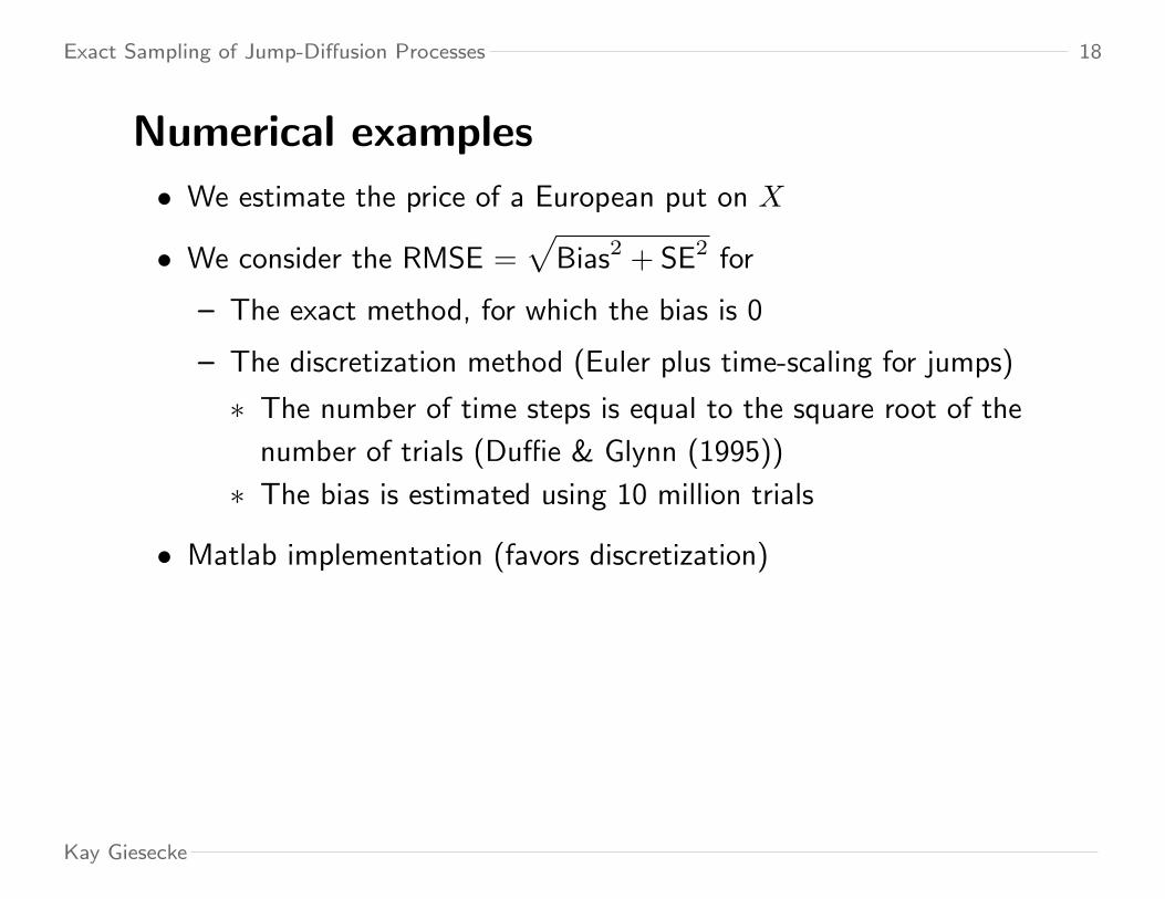
Numerical examples

• We estimate the price of a European put on X

• We consider the RMSE =√

Bias2 + SE2 for

– The exact method, for which the bias is 0

– The discretization method (Euler plus time-scaling for jumps)

∗ The number of time steps is equal to the square root of the

number of trials (Duffie & Glynn (1995))

∗ The bias is estimated using 10 million trials

• Matlab implementation (favors discretization)

Kay Giesecke


Numerical examples

X0 = 50, β = −1, r = 0.05, a = 50/4, b = 0, c = 0.5, T = 1, strike 5,

analytical value 0.1491

Method Trials Steps Value Bias SE RMSE Time (sec)

Exact 10K N/A 0.1417 0 0.00809 0.00809 36.19

Exact 20K N/A 0.1363 0 0.00561 0.00561 74.75

Exact 40K N/A 0.1522 0 0.00419 0.00419 150.52

Exact 100K N/A 0.1487 0 0.00262 0.00262 416.07

Exact 500K N/A 0.1495 0 0.00117 0.00117 1905.71

Euler 10K 100 0.1417 0.0019 0.00809 0.00831 26.72

Euler 20K 140 0.1496 0.0018 0.00587 0.00624 75.19

Euler 40K 200 0.1422 0.0008 0.00405 0.00413 215.75

Euler 100K 310 0.1531 0.0005 0.00265 0.00271 822.07

Euler 500K 707 0.1478 0.0004 0.00117 0.00123 9373.81

Kay Giesecke


Numerical ExamplesConvergence of RMSEs (log-log plot), strike K = 5

Kay Giesecke


Numerical examples

X0 = 50, β = −1, r = 0.05, a = 50/4, b = 0, c = 0.5, T = 1, strike 50,

analytical value 4.4118

Method Trials Steps Value Bias SE RMSE Time (sec)

Exact 10K N/A 4.3773 0 0.09309 0.09309 36.19

Exact 20K N/A 4.2248 0 0.06512 0.06512 74.75

Exact 40K N/A 4.4464 0 0.04781 0.04781 150.52

Exact 100K N/A 4.4123 0 0.02996 0.02996 416.07

Exact 500K N/A 4.4214 0 0.01344 0.01344 1905.71

Euler 10K 100 4.3198 0.0185 0.09345 0.09527 26.72

Euler 20K 140 4.451 0.0163 0.06742 0.06936 75.19

Euler 40K 200 4.3876 0.0157 0.04691 0.04946 215.75

Euler 100K 310 4.4464 0.0081 0.03031 0.03136 822.07

Euler 500K 707 4.3914 0.0039 0.01338 0.01394 9373.81

Kay Giesecke


Numerical ExamplesConvergence of RMSEs (log-log plot), strike K = 50

Kay Giesecke


Extensions

• The target functional can take the form

Ef((Xt)t∈S , (Jt)t≤T )

for a discrete set S of times t ∈ [0, T ]

– Treatment of certain path-dependent payoffs

• The intensity can take the form

λt = Λ(Xt−, Jt−, t)

Kay Giesecke


Conclusions

• We develop a method for the exact sampling of a one-dimensional

jump-diffusion process with state-dependent drift, volatility, jump

intensity and jump size

– Only mild conditions on the coefficients are required

• Numerical experiments indicate the advantages of the method

over a conventional discretization scheme

• Future research

– Efficiency: choice of localization bound

– Extension to multiple dimensions: stochastic volatility with

state-dependent jumps

Kay Giesecke

Exact Sampling of Jump-Di usion Processes Sampling of Jump-Di usion Processes 3 Jump-Di usion Fix a...

Documents

Transcript of Exact Sampling of Jump-Di usion Processes Sampling of Jump-Di usion Processes 3 Jump-Di usion Fix a...