Stochastic Modeling & Simulation of Reaction-Di usion ...
152
Stochastic Modeling & Simulation of Reaction-Diffusion Biochemical Systems Fei Li Dissertation submitted to the Faculty of the Virginia Polytechnic Institute and State University in partial fulfillment of the requirements for the degree of Doctor of Philosophy in Computer Science and Application Yang Cao, Chair John J. Tyson Layne T. Watson Adrian Sandu Samuel A. Isaacson December 4, 2015 Blacksburg, Virginia Keywords: stochastic simulation, reaction-diffusion systems Caulobacter crescentus Copyright c 2015, Fei Li
Transcript of Stochastic Modeling & Simulation of Reaction-Di usion ...

Stochastic Modeling & Simulation of Reaction-Diffusion
Biochemical Systems
Fei Li
Dissertation submitted to the Faculty of the
Virginia Polytechnic Institute and State University
in partial fulfillment of the requirements for the degree of
Doctor of Philosophy
in
Computer Science and Application
Yang Cao, Chair
John J. Tyson
Layne T. Watson
Adrian Sandu
Samuel A. Isaacson
December 4, 2015
Blacksburg, Virginia
Keywords: stochastic simulation, reaction-diffusion systems Caulobacter crescentus
Copyright c© 2015, Fei Li

Stochastic Modeling & Simulation of Reaction-Diffusion Biochemical
Systems
Fei Li
(ABSTRACT)
Reaction Diffusion Master Equation (RDME) framework, characterized by the discretization
of the spatial domain, is one of the most widely used methods in the stochastic simulation of
reaction-diffusion systems. Discretization sizes for RDME have to be appropriately chosen
such that each discrete compartment is “well-stirred” and the computational cost is not too
expensive.
An efficient discretization size based on the reaction-diffusion dynamics of each species is
derived in this dissertation. Usually, the species with larger diffusion rate yields a larger
discretization size. Partitioning with an efficient discretization size for each species, a mul-
tiple grid discretization (MGD) method is proposed. MGD avoids unnecessary molecular
jumpings and achieves great simulation efficiency improvement.
Moreover, reaction-diffusion systems with reaction dynamics modeled by highly nonlinear
functions, show large simulation error when discretization sizes are too small in RDME
systems. The switch-like Hill function reduces into a simple bimolecular mass reaction when
the discretization size is smaller than a critical value in RDME framework. Convergent Hill
function dynamics in RDME framework that maintains the switch behavior of Hill functions
with fine discretization is proposed.
Furthermore, the application of stochastic modeling and simulation techniques to the spa-
tiotemporal regulatory network in Caulobacter crescentus is included. A stochastic model
based on Turing pattern is exploited to demonstrate the bipolarization of a scaffold protein,
PopZ, during Caulobacter cell cycle. In addition, the stochastic simulation of the spatiotem-
poral histidine kinase switch model captures the increased variability of cycle time in cells
depleted of the divJ genes.

Acknowledgments
First and foremost, I would like to express my most deep gratitude to my family, who have
supported me all theses years on my way to pursuit my degree. Without their support, this
dissertation would not have been possible.
I’d like to give my sincere thanks to my advisor, Dr. Yang Cao, who guided me into this
exciting research area and encouraged me to explore my research interests. I have always
benefited from his knowledge, enthusiasm, patience, and constant support. I am also deeply
grateful to Dr. John J. Tyson for many valuable discussions and suggestions in my research. I
would like to thank the rest of my Ph.D. committee: Dr. Adrian Sandu, Dr. Layne T. Watson
and Dr. Samuel Isaacson, for their insightful suggestions and help for my dissertation.
I wish to express my heartful thanks to Dr. Kartik Subramanian for his splendid mathe-
matical model of Caulobacter crescentus. Last but not the least, I would like to give special
thanks to my labmates Yang Pu, Shuo Wang, Bo Peng and Minghan Chen for the enjoyable
office life. I’d like to send out my best wishes to the other friends, who have helped me and
lightened my life.
iii

Contents
1 Overview 1
2 Stochastic Simulation of Reaction-Diffusion Systems 6
2.1 Stochastic Simulation Algorithms . . . . . . . . . . . . . . . . . . . . . . . . 8
2.2 Stochastic Simulation of Reaction-Diffusion Systems . . . . . . . . . . . . . . 14
2.2.1 Particle-based Framework . . . . . . . . . . . . . . . . . . . . . . . . 15
2.2.2 Compartment-based Framework . . . . . . . . . . . . . . . . . . . . . 18
2.3 Reaction-Diffusion Master Equation in Microscopic Limit . . . . . . . . . . . 20
3 Efficient Discretization Size 24
3.1 Efficient Discretization Size . . . . . . . . . . . . . . . . . . . . . . . . . . . 25
3.2 Numerical Results . . . . . . . . . . . . . . . . . . . . . . . . . . . . . . . . . 28
3.2.1 Analytical Solution . . . . . . . . . . . . . . . . . . . . . . . . . . . . 29
3.2.2 Accuracy Estimation of Stochastic Simulation Results . . . . . . . . . 30
3.3 Conclusions . . . . . . . . . . . . . . . . . . . . . . . . . . . . . . . . . . . . 31
4 Multiple Grid Discretization Method 33
iv

4.1 Multiple Grid Discretization Method . . . . . . . . . . . . . . . . . . . . . . 34
4.2 Numerical Results . . . . . . . . . . . . . . . . . . . . . . . . . . . . . . . . . 36
4.2.1 MGD on A Simple 1D Toy Model . . . . . . . . . . . . . . . . . . . . 36
4.2.2 Stochastic Model of PopZ Polarization . . . . . . . . . . . . . . . . . 38
4.3 Discussion & Conclusion . . . . . . . . . . . . . . . . . . . . . . . . . . . . . 42
5 The Hill Function Dynamics in Reaction-Diffusion Systems 46
5.1 Hill Function Dynamics in Reaction-Diffusion Systems . . . . . . . . . . . . 47
5.2 Caulobacter Cell Cycle Modeling . . . . . . . . . . . . . . . . . . . . . . . . . 48
5.3 Hill Function Dynamics in Reaction-Diffusion Systems . . . . . . . . . . . . 49
5.4 Convergent Hill Function Dynamics with RDME . . . . . . . . . . . . . . . . 54
5.5 Conclusions . . . . . . . . . . . . . . . . . . . . . . . . . . . . . . . . . . . . 58
6 Stochastic Spatiotemporal Model of Response-Regulator Network in the
Caulobacter crescentus Cell Cycle 60
6.1 Background . . . . . . . . . . . . . . . . . . . . . . . . . . . . . . . . . . . . 61
6.2 Method . . . . . . . . . . . . . . . . . . . . . . . . . . . . . . . . . . . . . . 65
6.3 Results . . . . . . . . . . . . . . . . . . . . . . . . . . . . . . . . . . . . . . . 67
6.3.1 PleC Kinase Sequesters DivKp in the Early Predivisional Stage . . . 67
6.3.2 Compartmentalization Separates the Functionality of DivJ and PleC 69
6.3.3 DivK Overexpression . . . . . . . . . . . . . . . . . . . . . . . . . . . 69
6.3.4 DivJ Reduces the Variability in Swarmer-to-Stalked Transition Time 70
6.4 Discussion and Conclusion . . . . . . . . . . . . . . . . . . . . . . . . . . . . 72
v

7 Stochastic Simulation of PopZ Bipolarization Model in Caulobacter cres-
centus 74
7.1 PopZ Localization in Caulobacter Cell Cycle . . . . . . . . . . . . . . . . . . 75
7.2 Method . . . . . . . . . . . . . . . . . . . . . . . . . . . . . . . . . . . . . . 77
7.3 Stochastic Simulation Results . . . . . . . . . . . . . . . . . . . . . . . . . . 78
7.3.1 The two-gene model recreates PopZ bipolar distribution patterns . . 78
7.3.2 Turing pattern may account for the dynamic localization of FtsZ . . . 79
7.4 Conclusions . . . . . . . . . . . . . . . . . . . . . . . . . . . . . . . . . . . . 80
8 Outlook 81
8.1 Valid Stochastic Modeling of Nonlinear Dynamics in RDME Systems . . . . 82
8.2 ODE/SSA Hybrid Algorithms on Reaction-Diffusion System . . . . . . . . . 83
8.3 A hybrid framework Merging RDME and Smoluchowski Methods . . . . . . 83
8.4 Application: Stochastic Modeling and Simulation of Biological Models . . . . 84
A Supplement Materials 86
A.1 Transcription Factor Population at Equilibrium . . . . . . . . . . . . . . . . 86
B Supplement Materials 89
B.1 Model Details . . . . . . . . . . . . . . . . . . . . . . . . . . . . . . . . . . . 89
B.2 Reaction Channels and Propensities . . . . . . . . . . . . . . . . . . . . . . . 92
B.3 Result Figures . . . . . . . . . . . . . . . . . . . . . . . . . . . . . . . . . . . 103
C Supplement Materials 115
vi

C.1 Model Details . . . . . . . . . . . . . . . . . . . . . . . . . . . . . . . . . . . 115
C.2 Rule Based Modeling in Reaction Diffusion System . . . . . . . . . . . . . . 117
C.3 PopZ Reactions and Simulation Results . . . . . . . . . . . . . . . . . . . . . 118
C.4 FtsZ Reactions and Simulation Results . . . . . . . . . . . . . . . . . . . . . 120
Bibliography 121
vii

List of Figures
2.1 The schematic representation for discretization sizes h of RDME framework.
The traditional RDME has a upper bound hmax and lower bound hmin. Reac-
tion propensity correction is possible for discretization size in range (hmin, hcrit).
If the discretization size is smaller than the critical value hcrit, no local cor-
rection is possible. . . . . . . . . . . . . . . . . . . . . . . . . . . . . . . . . 23
3.1 Probability densities of molecular position of species B after the reaction fires in
the one-dimension model (3.4). Parameters: total length L = 1.0, kd = 0.1, and
D = 0.001. The efficient discretization size yields lc ≈ 0.04. The plot is generated
from 1,000,000 runs of stochastic simulations. . . . . . . . . . . . . . . . . . . . 30
3.2 The mean square errors of stochastic simulation with different discretization
sizes, compared with the theoretical solution (3.17). . . . . . . . . . . . . . 31
4.1 Multiple grid discretization of a reaction-diffusion system in one dimensional
domain of length L. The reaction dynamics of species Si gives an efficient
discretization size hi with Ki compartments, while species Sj has an efficient
discretization size hj, corresponding to Kj compartments. For simplicity, the
multiple grid discretization size hi = 3hj. . . . . . . . . . . . . . . . . . . . 34
viii

4.2 Population density of species C in the one dimensional spatial domain after time
t = 5.0. Parameters: total length L = 1.0, kA = 10.0, DA = 0.005, and Db = 0.5.
Initially, there is one molecule of A and one molecule of B in the center of the one
dimensional domain. The efficient discretization sizes are h(c)A = 0.1 and h
(c)B = 0.01.
The plot is generated from 100,000 runs of stochastic simulation. . . . . . . . . . 38
4.3 The spatioltemporal population level of the deterministic model (4.3). Colors
indicate population level, where red color means high population while blue
denotes low population level. . . . . . . . . . . . . . . . . . . . . . . . . . . 41
4.4 The stochastic reaction model and the reaction propensities for the PopZ
localization in a single compartment i. . . . . . . . . . . . . . . . . . . . . . 42
4.5 The spatiotemporal population evolution of PopZ polymer in the stochastic
simulation. The stochastic simulation results demonstrate that PopZ focus
polarizes in either end of the cell. . . . . . . . . . . . . . . . . . . . . . . . . 43
4.6 The firings of reaction and diffusion events with different discretization strate-
gies. Left: uniform discretization with discretization size h = 0.01 for both
species M and P. Right: multiple grid discretization with the efficient dis-
cretization sizes of 5% relative error. It is apparent that the firing number of
the diffusive jumps significantly decreases. . . . . . . . . . . . . . . . . . . . 45
5.1 The population oscillation of CtrAp during the Caulobacter crescentus cell
cycle. The left figure shows the deterministic model simulation result and the
right figure shows the stochastic model simulation result. In the swarmer stage
(t = 0− 30 min), the CtrA is phosphorylated and at a high population level,
which inhibits the initiation of chromosome replication. During swarmer-to-
stalk transition (t = 30−50 min), the CtrAp population quickly switches to a
low level, allowing the consequent initiation of chromosome replication in the
stalked stage. . . . . . . . . . . . . . . . . . . . . . . . . . . . . . . . . . . . 49
ix

5.2 A simple gene regulation model of Hill function dynamics in one dimensional
domain. Transcription factor (TF) is constantly synthesized and upregulates
the DNA expression. . . . . . . . . . . . . . . . . . . . . . . . . . . . . . . . 50
5.3 The histogram (left) and mean (right) population of mRNA with different
discretizations. Parameters: De = 1.0, ks = 2.5, kd = 0.1, ksyn = 5.0, kdeg =
0.05, system size L = 1.0. For the histogram figure, Km = 25.0. The log-log
plot shows the mean total mRNA population under different discretizations
and different parameter values. . . . . . . . . . . . . . . . . . . . . . . . . . 53
5.4 The total population of mRNA with different discretization sizes. Parameters:
system size L = 1.0, De = 1.0, ks = 2.5, kd = 0.1, ksyn = 5.0, kdeg = 0.05. For
the left figure Km = 25.0, while for the right figure Km = 50.0. . . . . . . . 56
5.5 The histogram and the mean population of mRNA with different discretization
sizes. Parameters: system size L = 1.0, De = 1.0, ks = 0.025, kd = 0.1,
ksyn = 0.05, kdeg = 0.05. For the left figure Km = 25.0, while for the right
figure Km = 50.0. . . . . . . . . . . . . . . . . . . . . . . . . . . . . . . . . 57
5.6 The comparison of CtrAp from the deterministic model and the stochastic
model simulation results. Left: CtrAp population trajectory during Caulobac-
ter crescentus cell cycle. Right: The histogram of the CtrAp population in
swarmer cells (t = 30 min). For model parameters, refer to Chapter 6. . . . 58
6.1 The asymmetric division cycle of Caulobacter cells. . . . . . . . . . . . . . . . . 61
6.2 Regulatory network of two phosphorelay systems that play major roles in the cell
division cycle of Caulobacter crescentus. The phosphorylated form of CtrA inhibits
the initiation of chromosome replication in swarmer cells. The phosphorylated form
of DivK indirectly inhibits the phosphorylation of CtrA, through the DivL–CckA
pathway. The kinase activity of the enzyme, PleC, is up-regulated by the product,
DivKp, of the kinase reaction. . . . . . . . . . . . . . . . . . . . . . . . . . . . 65
x
7.1 Demonstration of PopZ activity during Caulobacter cell cycle. PopZ focuses at
the old pole in swarmer cell and assumes bipolar localization later during the
cell cycle. ParB binds to PopZ at both poles, generating stable bipolarization
for further cell division. . . . . . . . . . . . . . . . . . . . . . . . . . . . . . 76
B.1 The transformations of PleC kinase and phosphatase when interacting with
DivK and DivKp. . . . . . . . . . . . . . . . . . . . . . . . . . . . . . . . . 104
B.2 Localization indicators for DivJ (upper left), PleC (upper right), DivL (lower
left) and CckA (lower right). The indicator functions = 0 (pink) or 1 (red). 105
B.3 Histograms of DivKp and free DivL in the early predivisional stage of the
Caulobacter cell cycle. Up: most DivKp molecules are complexed with PleC
histidine kinase. Bottom: Most DivL molecules are free to activate CckA kinase.106
xi

B.4 A typical stochastic simulation of regulatory proteins during the Caulobacter cell
cycle prior to cytokinesis. Colors indicate the numbers of protein molecules in each
bin. DivJ is synthesized throughout the cell cycle and becomes localized at the old
pole after t = 30 min. Transient co-localization of DivJ and PleC (t = 30−50 min)
turns PleC into kinase form, before PleC is cleared from the old pole (t = 50− 90
min) and relocates (t = 90 − 120 min) to the new pole (the nascent flagellated
pole). Upon phosphorylation, DivK localizes to the poles of the cell, where it binds
with PleC histidine kinase. Despite the presence of phosphorylated DivK at the
new pole of the predivisional cell, DivL stays active (free DivL, unbound to DivKp)
because PleC kinase sequesters DivKp and prevents it from binding to DivL. In the
swarmer stage, CckA is uniformly distributed and stays as the kinase form. In the
predivisional stage, CckA localizes to both poles. Reactivation of DivL turns CckA
into the kinase form at the swarmer pole, while CckA remains as a phosphatase
at the stalk pole. Consequently, the late predivisional cell establishes a gradient of
phosphorylated CtrA along its length with a high level of CtrAp at the new pole
and a low level at the old pole. Stochastic simulations generate temporally varying
protein distributions similar to the results of the deterministic model [106] with
realistic fluctuations superimposed. . . . . . . . . . . . . . . . . . . . . . . . . 107
B.5 A typical stochastic simulation of regulatory proteins in the late predivisional
stage of the Caulobacter cell cycle. Colors indicate the numbers of protein
molecules in each bin. The bold black line marks the division plane, which
separates the cell into two compartments. In the lower half (the stalked cell)
DivJ is actively phosphorylating DivK, which inhibits CtrA phosphorylation.
In the upper half (the nascent swarmer cell), there is insufficient DivKp to
keep PleC in the kinase form. As PleC transforms to phosphatase, it dephos-
phorylates DivKp. Consequently, DivL is activated and CtrAp accumulates
in the swarmer cell. . . . . . . . . . . . . . . . . . . . . . . . . . . . . . . . 108
xii

B.6 Representative stochastic simulations of cells that overexpress DivK two-fold.
Some cells complete the cell cycle normally (up), while most cells stall in the
stalked stage (bottom). . . . . . . . . . . . . . . . . . . . . . . . . . . . . . 109
B.7 Histogram of total phosphorylated CtrA in the early predivisional stage.
Stochastic simulations show that some cells have a high population of CtrAp,
which enables them to complete the cell cycle as a wild-type cell would, while
others stay in the stalk stage and fail to divide. . . . . . . . . . . . . . . . . 110
B.8 The average level (over 250 stochastic simulations) of total CtrAp in the case of
four-fold DivK overexpression (up) and eight-fold DivK overexpression (bot-
tom). . . . . . . . . . . . . . . . . . . . . . . . . . . . . . . . . . . . . . . . 111
B.9 Histograms of CtrAp populations at t = 30 min. With eight-fold DivK over-
expression, CtrA phosphorylation is greatly reduced in what should be the
swarmer stage of the cell cycle. . . . . . . . . . . . . . . . . . . . . . . . . . 112
B.10 Typical trajectories of the total numbers of CtrAp molecules during a wild-
type cell cycle. CtrAp populations are high in the swarmer stage and drop
dramatically at the swarmer-to-stalked transition, to allow the initiation of
chromosome replication. . . . . . . . . . . . . . . . . . . . . . . . . . . . . . 112
B.11 Histograms of swarmer-to-stalked transition times in wild-type cells and ∆divJ
mutant cells. The mean transition time is ∼ 42 min for wild-type cells and
∼ 49 min for ∆divJ mutant cells. ∆divJ mutant cells show a much larger
variance of transition times. The coefficient of variation of swarmer-to-stalked
transition times is 14% for wild-type cells and 29% for ∆divJ cells, in very
good agreement with the COVs observed by Lin et al. [68] for total cell cycle
times. We conclude that depletion of divJ doesn’t stall the swarmer-to-stalked
transition for long, but it causes large fluctuations in the transition time. . . 113
B.12 Histograms of DivKp at t = 50 min in wild-type and ∆divJ cells. . . . . . . 113
xiii
B.13 Histogram of PleC kinase at t = 50 min in wild-type and ∆divJ cells. . . . 114
B.14 Histogram of CtrAp at t = 50 min in wild-type and ∆divJ cells. . . . . . . 114
C.1 Stochastic simulation result of PopZ polarization model. Up left: One popZ
gene is constantly present at 20% of cell length from the old pole end. The
chromosome replication starts at t = 50 min and the replicated chromosome
translocates across the cell until it reaches the position of 20% cell length from
the new pole end. Up right: popZ mNRA is synthesized from the two genes.
Due to the short life time (half life time of 2 ∼ 3 min) and slow diffusion
(0.05µm2/min), mNRA can not move far from popZ gene site. Bottom: PopZ
shows a unipolar-to-bipolar transition at around t = 75 min. . . . . . . . . . 122
C.2 Histogram of time (top) and cell length (bottom) when popZ gene segregation
is complete (green) and PopZ becomes bipolar (red). . . . . . . . . . . . . . 123
C.3 The spatiotemporal pattern of stochastic simulation on FtZ polarization model.
Up: MipZ assembles the distribution of PopZ. MipZ binds to the chromosome
front in swarmer cells. After the chromosome segregation stars, MipZ translo-
cates to the new pole together with the replicated chromosome. Bottom: In
the swarmer cell, MipZ stays in the old pole and repels FtsZ polymers to the
new pole. After the chromosome segregation completes, FtsZ shifts towards
the middle of the cell, where MipZ level is lowest. . . . . . . . . . . . . . . . 124
xiv

List of Tables
1.1 Cell Sizes and Protein Populations of Several Typical Species . . . . . . . . . 2
4.1 Propensity functions for some typical chemical reactions of the multiple grid
discretization as in figure 4.1 . . . . . . . . . . . . . . . . . . . . . . . . . . 35
4.2 Comparison of stochastic simulation with different discretization strategies . 39
4.3 Parameters of PopZ localization model. The parameter unit is estimated in
population number. . . . . . . . . . . . . . . . . . . . . . . . . . . . . . . . . 40
4.4 The efficient discretization sizes for PopZ monomers and polymers . . . . . . 43
4.5 Firing numbers of reaction/diffusion events and simulation CPU time for dif-
ferent discretization strategies . . . . . . . . . . . . . . . . . . . . . . . . . . 44
6.1 The mean and variance of the swarmer-to-stalked transition times in wild-type
and divJ deletion cells. . . . . . . . . . . . . . . . . . . . . . . . . . . . . . . 72
B.1 Chemical reactions and propensities in the Response-Regulator Model . . . . 92
B.2 Diffusive reactions and propensities in the Response-Regulator Model . . . . 102
C.1 Chemical reactions and propensities of PopZ . . . . . . . . . . . . . . . . . . 118
C.2 Chemical reactions and propensities of FtsZ . . . . . . . . . . . . . . . . . . 120
xv

Chapter 1
Overview
Reaction-diffusion systems, such as biochemical cell cycle regulation models [42, 106], ecosys-
tems [34] and pattern formation models [105, 59, 111], widely exist in nature. Classic studies
have been exploiting deterministic differential equations (PDEs and ODEs) to model the
reaction dynamics of these systems. Deterministic models are powerful tools to study qual-
itative evolution and bifurcation dynamics of reaction-diffusion systems.
Differential equation modeling approaches assume the concentrations of all species in a
reaction-diffusion system are continuous and evolve deterministically. However, in reality
biological systems are always subject to external noise from signal stimuli and environmental
perturbations. Furthermore, the size of a cellular system is so small that species populations
in a cell are discrete and limited [107, 86]. For instance, the volume of a Caulobacter cell is
roughly 1 fL ∗ at division and contains about 300 molecules of a particular protein species (if
its concentration is 500 nmol/L). Moreover, the number of mRNA molecules for each protein
at any time is likely to be about 10 [107]. With such small numbers of mRNAs and proteins,
molecular fluctuations at the protein level are expected to be around 25% [86]. Such large
fluctuations in protein levels may significantly affect the properties of the cell cycle control
system. In addition, experimental data at single-cell level demonstrates considerable vari-
∗femto- (f) is a unit prefix in the metric system denoting a factor of 10−15. 1 fL = 10−15 L.
1

2
Table 1.1: Cell Sizes and Protein Populations of Several Typical Species
Cell Cycle Time Cell Size Population of a Signaling Protein
(minutes) (µm3) (molecules/cell)
E. coli 20 ∼ 40 0.5 ∼ 5 10 ∼ 1000
S. cerevisiae 70 ∼ 140 20 ∼ 160 500 ∼ 30000
Hela 900 ∼ 1800 500 ∼ 5000 104 ∼ 106
ability from cell to cell. Table 1.1 shows some characteristic features of bacteria, yeast and
human cells.
Therefore, stochastic models and simulation algorithms have been proposed to capture the
intrinsic noise in cellular reaction-diffusion systems [44, 2, 112, 84]. The stochastic mod-
eling strategies can be categorized into two theoretical frameworks: the continuous-space
discrete-time particle-based framework, such as the Smoluchowski model [114], and the time-
continuous compartment-based framework, such as the Reaction-Diffusion Master Equation
(RDME) [32, 83] framework. In the particle-based framework, molecules are modeled as
Brownian particles that diffuse in continuous-space domain. In each small time step, a
chemical reaction fires if the next reaction time is less than the time step. The positions
of all diffusive molecules are updated according to Brownian dynamics. For a bimolecular
reaction, when two reactant molecules are within a distance of “reaction radius” [20, 57],
the bimolecular reaction fires with a fixed propensity density or instantaneously (reaction
propensity approaches infinity) [114]. Higher order reactions, such as trimolecular reactions,
are considered unrealistic and are not studied in particle-based models. Particle-based frame-
work resolves the exact positions of molecules and is mathematically fundamental. Though,
particle-based framework requires high computation costs for large systems.

Chapter 1. Overview 3
RDME framework is characterized by the discretization of spatial domains, with the as-
sumption that molecules are “well-stirred” within each compartment. Chemical reaction
dynamics in each compartment are governed by Chemical Master Equations (CMEs) [77, 37]
and diffusion is modeled as random walk of the species molecules between neighboring com-
partments. Compartment-based models are coarse-grained and better suited for large scale
simulations [27]. Typically, the spatial discretization size of a reaction-diffusion system has
to be appropriately chosen such that within each compartment, molecules are “well-stirred”
and the computational cost is not too expensive. There have been many research studies on
the discretization strategies, such as the uniform 1-D discretization [60, 10] adaptive meshes
and unstructured meshes [5] for non-uniform 1-D discretization.
In a “well-stirred” compartment, it is not necessary to track the detailed positions of every
molecule. A “well-stirred” biochemical system can be defined by the instantaneous popu-
lations of various species alone. Chemical reaction dynamics of a “well-stirred” system are
fully governed by Chemical Master Equations (CMEs). CME is a set of ODEs that gives
one equation for every possible combination of species populations. Therefore, it is both
theoretically and computationally intractable to solve CMEs for most practical biochemical
systems due to the huge number of possible system states. Stochastic simulation methods
are then exploited to construct realizations of state trajectories.
Gillespie’s Stochastic Simulation Algorithm (SSA) [36] is one of the most widely used sim-
ulation methods for stochastic simulations of “well-stirred” systems. There exist several
implementations of SSA, such as direct method [36], first reaction method [36], next reac-
tion method [33], optimized direct method [14] and the constant-time SSA [101]. SSA is
computationally intensive for most practical models. Much effort has been focused on the
simulation efficiency improvement. Furthermore, researchers have developed several approx-
imation algorithms for particular biochemical systems, such as τ -leaping method [39, 41],
quasi-steady-state SSA [93] and slow scale SSA [12]. Also, the merging of stochastic sim-
ulation with deterministic modeling for multiscale systems brings up a hybrid SSA/ODE
method [43, 70].

4
In the compartment-based framework, discretization yields “well-stirred” compartments.
The improvement over SSA can also be applied to stochastic simulations of reaction-diffusion
systems. In addition, novel improvements have been proposed in the effort to alleviate the
computational cost on molecular random walks. The binomial tau-leap spatial stochastic
simulation algorithm [72] combines the idea of aggregating diffusive transitions with the pri-
ority queue structure. Additionally, a novel formulation based on the finite state projection
(FSP) method [82], called diffusive FSP (DFSP) method [22], has been developed for efficient
and accurate simulation of diffusive processes.
Traditional discretization sizes of RDME have upper and lower bounds. It has been well
established that the discretization size should be smaller than mean free paths of all reactant
molecules for each compartment to be considered “well-stirred” [4]. Furthermore, it has been
proved that when discretization sizes approach zero in high dimensional domains, simulation
of bimolecular reactions leads to great errors. As a result, RDME becomes divergent and
yields unphysical results [52, 26, 45].
This dissertation focuses on the mathematical analysis of stochastic models and the devel-
opment of efficient stochastic simulation algorithms for reaction-diffusion systems. A math-
ematical formula of efficient discretization size in RDME framework is derived in Chapter 3.
This formula usually yields larger discretization sizes for species with larger diffusion rates.
Discretizing the spatial domain for each species based on its corresponding discretization
size, a multiple grid discretization (MGD) method is proposed in Chapter 4. Experiments
with a toy model and a Turing pattern based model demonstrate that MGD greatly improves
the simulation efficiency with a controllable relative error tolerance.
Moreover, numerical analysis of Hill function reaction laws in reaction-diffusion systems
demonstrates that the switching behavior of Hill dynamics reduces into a simple bimolec-
ular reaction dynamics when the spatial discretization size is small enough. Furthermore,
following the work of convergent Reaction Diffusion Master Equation (CRDME) [53], a con-
vergent Hill function simulation scheme in the microscopic RMDE framework is presented

Chapter 1. Overview 5
in Chapter 5.
In addition to the theoretical analysis, stochastic modeling and simulation of regulatory
networks in Caulobacter crescentus cell cycle are included in Chapter 6 and Chapter 7. A
stochastic model of the histidine kinase regulatory network model during the Caulobacter
crescentus cell cycle is addressed in Chapter 6. The stochastic model takes into account
molecular fluctuations of the regulatory proteins in space and time during early stages of the
cell cycle of wild-type Caulobacter cells. Moreover, stochastic simulations match with the
experimental observations of increased variability of cycle time in cells depleted of the divJ
gene. In addition, stochastic simulations suggest that a small fraction of the mutants cells
do complete the cell cycle normally in the scenarios of divK gene overexpression.
In addition, experimental results show that the cytoplasm of Caulobacter crescentus not only
changes with time, but also is elaborately organized in space during the cell cycle process [18].
The spatiotemporal cell cycle control of Caulobacter has attracted much attention in the
research of location regulation in prokaryotic cells. A scaffold protein, PopZ, in Caulobacter
becomes bipolar and promotes the localization of several other regulatory proteins during its
cell cycle. A Turing pattern mechanism is exploited to study the bipolarization of PopZ. A
stochastic model, presented in Chapter 7, demonstrates the PopZ polarization and captures
the variability in the cell length and time when PopZ becomes bipolar.

Chapter 2
Stochastic Simulation of
Reaction-Diffusion Systems
Classic studies on chemical reaction dynamics often use deterministic differential equations
(ODEs and PDEs) to model molecular concentration changes of spatiotemporal biological
systems. Traditional chemical dynamical models assume that species concentration is a
continuous variable and evolves deterministically. The evolution of molecular concentration
ui for species Si, i = 1, 2, . . . , N , is formulated as
∂ui∂t
= Di∆ui + fi(u1, u2, . . . , uN), (2.1)
where Di indicates the diffusion constant of species Si and the chemical reaction function fi
is inferred from reaction dynamics. The Laplace operator ∆ denotes the sum of all unmixed
second partial derivatives in Cartesian coordinates:
∆u =n∑i=1
∂2
∂x2i
u. (2.2)
The traditional chemical reaction dynamics are valid when all species present with enormous
number of population. However, a cellular system is so small that the molecular populations
of particular protein species are limited to magnitude of several hundreds or thousands [74,
6

Chapter 2. Stochastic Simulation of Reaction-Diffusion Systems 7
28, 97]. “Concentration” changes are no longer continuous and population discreteness
and stochasticity may play critical roles. Therefore, deterministic equations (2.1) are not
applicable to model the chemical kinetics of such small systems. The ultimate approach to
depict the time evolution of chemical reaction systems is to meticulously track the molecular
positions and populations for all chemical species [40].
When a chemical system is “well-stirred”, all the molecules of the same species are spatially
indistinguishable and it is not necessary to track their detailed positions. A “well-stirred”
system can be defined by the instantaneous molecular populations of various species alone.
When diffusion is not fast enough such that the chemical system is not “well-stirred”, molec-
ular motion and spatial information can not be neglected. In general, stochastic modeling
methods [44, 2, 112] to model reaction-diffusion systems can be categorized into two distinct
frameworks. One is the continuous-space particle-based framework, such as the Smolu-
chowski model [114]. In the Smoluchowski model, each molecule has a precise location. Dif-
fusion is modeled as the spatially continuous Brownian motion of individual molecules [26].
In each step, the Smoluchowski model checks whether a reaction fires during a small time
period. The Smoluchowski framework precisely tracks the position of every molecule and
is better to represent the microscopic physics of reaction-diffusion systems. However, when
the numbers of species populations and reaction channels are large, the Smoluchowski model
becomes impractical and hard to keep track of every molecule and every reaction channel.
The second class of models is often referred to as the compartment-based framework [32, 83],
which is characterized by the discretization of the spatial domain. One example is the
Reaction Diffusion Master Equation (RDME), where molecules in each discrete compartment
are considered “well-stirred”. Diffusion is modeled as random walk of species molecules
between adjacent compartments. Within each “well-stirred” compartment, chemical reaction
dynamics are described by Chemical Master Equations (CMEs) [77, 37]. RDME framework
is preferred in the modeling of large reaction-diffusion systems [31].
In addition to these two typical frameworks, a hybrid model, integrating compartment-

8
based method with molecular-based method has been developed [31]. In this framework,
molecular-based model is used for localized regions where accurate and microscopic details
are important and compartment-based framework is used where accuracy can be trade for
simulation efficiency.
In this chapter, a brief review of the mathematical background on stochastic simulation
of “well-stirred” chemical reaction systems and the two stochastic simulation frameworks
for the reaction-diffusion systems is presented. Furthermore, an assessment regarding the
limitations and future development of stochastic modeling and simulation is included.
2.1 Stochastic Simulation Algorithms
Consider a well-stirred biochemical system of N species S1, S2, . . . , SN interacting through
M reaction channels R1, R2, . . . , RM within a constant volume Ω. The instantaneous state
of the chemical system is determined by the state vector X(t) ≡ [X1(t), X2(t), . . . , XN(t)]T ,
where Xi(t) is the number of molecules for species Si at time t. The state vector defines the
biochemical system at each time point and the state changes only when a chemical reaction
fires. Each chemical reaction channel Rj is characterized by the propensity function aj(x)
and the state change vector νj . The propensity function aj(x) is defined as
aj(x)dt ≡ probability that one Rj reaction occurs
in the next infinitesimal time interval [t, t+ dt),
given X(t) = x.
(2.3)
The state change vector νj ≡ [ν1j, ν2j, . . . , νNj]T gives the molecular population changes of
every species Si, induced by one Rj reaction. The matrix ν = [ν1,ν2, . . . ,νM ] is also referred
to as stoichiometric matrix.
Once the propensity functions and stoichiometric matrix are determined, Chemical Master
Chapter 2. Stochastic Simulation of Reaction-Diffusion Systems 9
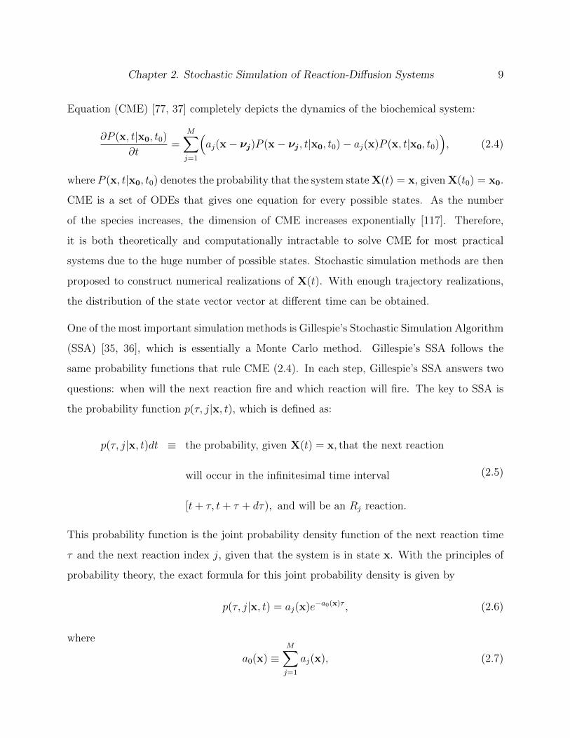
Equation (CME) [77, 37] completely depicts the dynamics of the biochemical system:
∂P (x, t|x0, t0)
∂t=
M∑j=1
(aj(x− νj)P (x− νj , t|x0, t0)− aj(x)P (x, t|x0, t0)
), (2.4)
where P (x, t|x0, t0) denotes the probability that the system state X(t) = x, given X(t0) = x0.
CME is a set of ODEs that gives one equation for every possible states. As the number
of the species increases, the dimension of CME increases exponentially [117]. Therefore,
it is both theoretically and computationally intractable to solve CME for most practical
systems due to the huge number of possible states. Stochastic simulation methods are then
proposed to construct numerical realizations of X(t). With enough trajectory realizations,
the distribution of the state vector vector at different time can be obtained.
One of the most important simulation methods is Gillespie’s Stochastic Simulation Algorithm
(SSA) [35, 36], which is essentially a Monte Carlo method. Gillespie’s SSA follows the
same probability functions that rule CME (2.4). In each step, Gillespie’s SSA answers two
questions: when will the next reaction fire and which reaction will fire. The key to SSA is
the probability function p(τ, j|x, t), which is defined as:
p(τ, j|x, t)dt ≡ the probability, given X(t) = x, that the next reaction
will occur in the infinitesimal time interval
[t+ τ, t+ τ + dτ), and will be an Rj reaction.
(2.5)
This probability function is the joint probability density function of the next reaction time
τ and the next reaction index j, given that the system is in state x. With the principles of
probability theory, the exact formula for this joint probability density is given by
p(τ, j|x, t) = aj(x)e−a0(x)τ , (2.6)
where
a0(x) ≡M∑j=1
aj(x), (2.7)

10
denotes the total reaction propensity of all reaction channels. Equation (2.6) is the math-
ematical basis of SSA approaches. It implies that the time τ to the next reaction is an
exponential random variable with mean and standard deviation 1/a0(x), while the reac-
tion index j is a statistically independent integer random variable with point probability
aj(x)/a0(x).
There are several Monte Carlo procedures for generating samples of τ and j according to
their distributions. The simplest is the so called “direct method” [35, 36, 40], which generates
two uniformly distributed random numbers r1 and r2 in the unit interval (0, 1), and takes
τ =1
a0(x)ln(
1
r1
),
j = the smallest integer satisfying
j∑j′=1
aj′(x) > r2a0(x).
(2.8)
The biochemical system is then updated according to X(t+ τ) = X(t) + νj. This process is
repeated until the simulation end criterion is reached.
An equivalent implementation to “direct method” is the so called “first reaction method”
(FRM) [35, 36]. With probability theory, it is easy to formulate the probability for one Rj
reaction to fire in time interval [t+ τ, t+ τ + dτ) as
pj(τ)dτ = aj(x, t) · e−aj(x,t)τdτ, (2.9)
if no other reactions alter the reactant population of reaction Rj. The first reaction method
generates a “potential reaction time” for each reaction channel and fires the reaction that
has the smallest firing time. In accordance with the reaction probability equation (2.9), the
reaction time for reaction channel Rj can be formulated as
τj =1
aj(x)ln(
1
rj), (j = 1, 2, . . . ,M), (2.10)
with each rj a uniform random variable in (0, 1). First reaction method (FRM) is as rigorous
as the direct method, though, FRM is much less efficient than the direct method. FRM
generates M random reaction times and calculate M logarithms in each step, while the
direct method only requires one random variable and one logarithm operation.

Chapter 2. Stochastic Simulation of Reaction-Diffusion Systems 11
A reformulation of SSA, which significantly improves the simulation efficiency for large bio-
chemical systems, is Gibson and Bruck’s next reaction method (NRM) [33]. Next reaction
method introduces a dependent graph to record the influence of one reaction channel over
other reaction channels. Moreover, the absolute potential reaction times for all reaction
channels are maintained in a priority queue. Hence, the time and index of the next reaction
is always available at the top of the priority queue. If the reaction propensities of some
reactions are not affected by one firing of the top reaction, the same expected reaction times
forward to the next step. Next reaction method devises a clever formula to update the ex-
pected reaction time for those reactions whose propensities are changed by firing of the top
reaction. With these elaborate design, the next reaction method is significantly faster than
the first reaction method and is even faster than the direct method for some simple systems.
“Optimized Direct Method” (ODM) [14] adopts the dependent graph in NRM and rear-
ranges reaction channel indices according to reaction firing frequencies. The dependent
graph avoids unnecessary propensity calculations. Furthermore, with the reaction channel
indices rearranged, where the more frequently firing reaction channels are indexed before
the less frequent ones, the average search steps for the firing reaction channel is minimized.
“Optimized Direct Method” starts off with several sample runs to collect the average firing
frequency, according to which the reaction channels are reindexed. With these improve-
ments, “Optimized Direct Method” becomes one of the most efficient SSA implementation
strategies.
In order to dynamically adjust reaction channel indices, sorting direct method (SDM) [75]
is proposed. In SDM, the reaction channel index decreases by one whenever a reaction
fires. This reindexing strategy makes the reaction indices converge to an optimized one
after certain simulation time. This tactic not only eliminates the requirement of preruns as
in ODM, but also accommodates the relative propensity changes that may develop as the
simulation proceeds.
More recently, logarithm direct method (LDM) [65] and constant-time SSA [101] are de-

12
veloped. LDM applies binary search over the partial sum of reaction propensities and is
often more efficient than direct method for very large systems. Constant-time SSA uses a
particular random variate generation (RVG) algorithm known as composition and rejection.
Constant-time SSA assumes that the ratio of the maximum reaction propensity pmax to the
minimum reaction propensity pmin is bounded. In the composition stage, it groups reactions
by cascading reaction propensity segments pmin, 2pmin, 4pmin, . . . , 2Npmin. For a practical
system, pmax/pmin ratio is bounded and the number of groups is also bounded. Therefore,
random selection of a reaction group can be considered a constant time operation. Once a
group is selected, on average, selection of the firing reaction within each group requires less
than two iterations of “rejection” procedures, since all the reaction propensities in group
g are between 2gpmin and 2g+1pmin. Constant-time SSA proves to be competitive even for
small networks, and performs significantly faster as the size of a biochemical system grows
larger.
Despite such improvement, SSAs are computationally intensive for many realistic problems,
particularly when one has to run the simulation many times to collect ensemble data. Alter-
native to pursuing exact SSAs, several efficient approximation simulation strategies, which
gain efficiency improvement by trading off certain simulation accuracy, have been developed.
Tau-leaping method [39, 41] speeds up stochastic simulation by leaping over many reactions
in one time step. Tau-leaping method chooses a small τ value such that over time step τ , no
reaction propensity changes significantly. At each time step, tau-leaping method [39] samples
the firing number of reaction channel Rj by Poisson random variable generator of mean and
variance aj(x)τ . In order for tau-leaping to be practical, many elaborate procedures for
quickly determining time step τ have been proposed [38, 39, 40, 13, 15].
For real chemical systems, reactions often fire on vastly different time scales. An exact
stochastic simulation spends most of time on simulating fast reacting events, which is frus-
tratingly inefficient since fast reacting events are often of much less significance than slow
reacting events. The quasi-steady-state assumption on high-population variables [93] and

Chapter 2. Stochastic Simulation of Reaction-Diffusion Systems 13
the partial equilibrium assumption on fast (high propensity) reactions [12] have been applied
on stiff systems to accelerate the simulation.
Moreover, several hybrid methods that merge the simulation methods of stochastic SSA and
deterministic ODE based on multiscale features of real biochemical systems have been pro-
posed [43, 95, 12]. Haseltine and Rawlings [43] propose to partition a biochemical system into
groups of slow and fast reactions. The partitioning criterion is determined by two thresh-
olds, i.e. propensity threshold and population threshold, set by users before simulation. A
reaction is considered to be fast if its propensity is greater than the propensity threshold and
the populations of its reactants are greater than the population threshold. In Haseltine and
Rawlings’s hybrid method, fast reactions are governed by ODEs or CLEs and slow reactions
are simulated by Gillespies direct method. A similar strategy is adopted by Salis [95, 96]
where fast reactions are approximated by CLEs and slow reactions are simulated by Gib-
son and Brucks next reaction method [33]. Cao proposes to partition a biochemical system
based simply on species population numbers [12]. For species whose population numbers
are less than a threshold, all related reactions are simulated by SSAs, while other reactions
are simulated by tau-leaping method. An aggressive partition strategy, where only reactions
with low populations as well as low propensities are simulated by SSA methods, while others
are modeled by ODEs, is also proposed [70].
With the aggressive partition strategy, all reaction channels are grouped into two subsets:
Sfast for “fast” reactions and Sslow for “slow” reactions. Let ai(x, t) be the propensity of the
ith reaction channel in Sslow, τ be the jump interval of the next stochastic reaction, and j
be its reaction index. The improved hybrid algorithm solves for τ and j as follows.
Algorithm Improved SSA/ODE Hybrid Method
1. Generate two uniform random numbers r1 and r2 in U(0, 1).
2. Integrate the ODE system and solve for τ ,∫ t+τ
t
atot(x, t)dt+ log(r1) = 0, (2.11)

14
where atot(x, t) is the total propensity of slow reactions Sslow .
3. Determine j as the smallest integer satisfying
j∑j′=1
aj′(x, t) > r2atot(x, t). (2.12)
4. Update X(t) according to the state change vector of the jth reaction in Sslow .
5. Go to step 1 until stopping condition is reached.
Solving equation (2.11) is an important step, particularly when slow reaction propensities
change appreciably over time according to fast reaction dynamics. The integration in equa-
tion (2.11) is easy to be formulated as a differential equation, by adopting a variable z,
dz
dt= atot(x), (2.13)
with the initial condition at τ = 0,
z(t) = − log(r1).
At every simulation step, starting from time t, the differential equation (2.13) is numerically
integrated until z(t+τ) = 0. Then, τ gives the solution for equation (2.11). This integration
can be performed by a standard ODE solver with root-finding, such as LSODAR [46, 92].
2.2 Stochastic Simulation of Reaction-Diffusion Sys-
tems
Diffusion is the result of random migrations of molecules. There are two ways to study
diffusion: either a phenomenological approach by Fick’s law or a physical study through
Brownian motion. Fick’s law [29, 30] relates the diffusive flux to the concentration gradient
and further predicts the concentration change caused by diffusive flux. The diffusion equation
by Fick’s law reads∂u(x, t)
∂t= D∆u(x, t), (2.14)

Chapter 2. Stochastic Simulation of Reaction-Diffusion Systems 15
where D is the diffusion constant, u(x, t) is the molecular concentration at position x and
∆ is the Laplace operator.
A century after the discovery of Brownian motion, Einstein formulated the mathematical
expression of Brownian motion [24]. With the mathematical formula of Brownian motion,
Einstein is the first to realize that the mean displacement of a Brownian particle is in-
significant, instead, the basic quantity character of Brownian motion is the mean square
displacement.
Suppose a Brownian particle starts at the origin of a Euclidean coordinate system. Then the
solution to Equation (2.14) gives the probability density of the displacement at any time t,
f(x, t) =1
(√
4πDt)de−‖x‖24Dt , (2.15)
with d the dimension of the spatial domain concerned. Equation (2.15) shows that the
displacement at time t is a normal distribution with mean zero, while the arithmetic mean
of the squares of displacement is given by
〈‖x(t+ ∆t)− x(t)‖2〉 = 2dD∆t. (2.16)
Based on different modeling schemes for diffusion, different modeling techniques for reaction-
diffusion systems have been developed. The next part briefly addresses the two major
stochastic simulation frameworks for reaction-diffusion systems.
2.2.1 Particle-based Framework
The particle-based framework fastidiously keeps track of the positions of every molecule.
The trajectory of an individual molecule is computed according to the displacement distri-
bution (2.15) of Brownian particles. At a small time step ∆t, the position of each molecule

16
is update by
x(t+ ∆t) = x(t) +√
2D∆tξx,
y(t+ ∆t) = y(t) +√
2D∆tξy,
z(t+ ∆t) = z(t) +√
2D∆tξz,
(2.17)
where ξx, ξy and ξz are independent random variables sampled from standard normal distri-
bution with zero mean and unit variance.
For each possible reaction channel, the firing time for the next reaction is sampled according
to equation (2.10). If the firing time of reaction Rj is less than the time step ∆t, then a Rj
reaction fires before another molecular position update. For a zeroth or first order reaction,
the reaction propensity calculation is similar as in “well-stirred” systems.
For bimolecular reactions, two reactant molecules fire a reaction with constant propensity
λ when the distance of two reactant molecules fall into a reaction radius ρ. This reaction
model is often referred to as the ρ− λ model [26].
Consider a bimolecular reaction with reactant species A and B, producing a new species C.
A+Bk−→ C. (2.18)
The molecules of A and B diffuse freely with diffusion constant DA and DB, respectively.
When a molecule of A diffuses to the ball of radius ρ centered in a B molecule, the bimolecular
reaction fires with propensity λ.
Suppose a coordinate system with the origin being the center of the ball. c(r) denotes the
equilibrium concentration of species A at distance r from the origin. With only one molecule
of A, the concentration is essentially the probability density of occurrence for molecule A at
position r. The concentration c(r) can be profiled as [69]d2c
dr2+
2
r
dc
dr= 0, r ≥ ρ,
d2c
dr2+
2
r
dc
dr− cλ
DA +DB
= 0, r < ρ,
(2.19)

Chapter 2. Stochastic Simulation of Reaction-Diffusion Systems 17
with the boundary condition at infinity as
limr→∞
c(r) = c∞. (2.20)
At the ball boundary r = ρ, species concentration c is continuous and differentiable. Thus,
differential equation (2.19) yields a unique solution
c(r) =
c∞ +
a1
r, r ≥ ρ,
2a2
rsinh
(r
√λ
DA +DB
), r < ρ,
(2.21)
with the constant variables
a1 = c∞
(√(DA +DB)/λ tanh
(ρ√λ/(DA +DB)
)− ρ),
a2 = c∞√
(DA +DB)/λ(
2 cosh(ρ√λ/(DA +DB)
))−1
.
(2.22)
The flux across the ball boundary of reaction radius is
Φ = 4πρ2(DA +DB)∂c
∂r
∣∣∣∣r=ρ
= 4π(DA +DB)c∞
(ρ−
√(DA +DB)/λ tanh
(ρ√λ/(DA +DB)
)).
(2.23)
The flux across the boundary of reaction radius represents the bimolecular reaction rate in
the microscopic perspective. Equivalently, the classic study of chemical reaction dynamics
concludes that the reaction rate of a bimolecular reaction is given by a reaction rate constant
k multiplied by the species concentration far away from the molecular center, c∞. Therefore,
the reaction rate constant k for bimolecular reaction is formulated by
k = 4π(DA +DB)(ρ−
√(DA +DB)/λ tanh
(ρ√λ/(DA +DB)
)). (2.24)
In the case λ → ∞, where the two reactant molecules react instantaneously when they fall
into the distance of reaction radius ρ, Equation (2.24) reduces to
k = 4π(DA +DB)ρ. (2.25)

18
On the other hand, if λ is small enough such that λ (DA +DB)/ρ2, Equation (2.24) can
be simplified as k ≈ 4πρ3λ/3, which can be rewritten as
λ ≈ k
4πρ3/3. (2.26)
Equation (2.26) indicates that the bimolecular reaction rate λ is the macroscopic reaction
rate constant k divided by the volume of reaction ball, when the reaction ball is sufficiently
large.
Particle-based frameworks consider high order reactions physically unrealistic and are not
applicable to systems with high order reactions. Furthermore, it is important to realize
that the time step ∆t in molecular-based models must be small enough such that λ∆t 1
for all the chemical reactions. By the typical parameter values for protein interactions in
biological systems, the time step ∆t has to be significantly less than a nanosecond [26]. To
get around the small time step limit, event-driven algorithms are developed. The Green’s
Function Reaction-Diffusion (GFRD) algorithm [112] uses a maximum time step until a
single reaction fires. In GFRD, Smoluchowski equations for molecular diffusion are solved
analytically using Green’s functions, and the system advances to the time point when a
reaction event occurs. GFRD is often up to 5 orders of magnitude faster than conventional
Smoluchowski schemes for real biologically systems [113].
2.2.2 Compartment-based Framework
Assume in a spatial domain Ω of one dimension, there exist N species S1, S2, ..., SN,
interacting through M reaction channels R1, R2, . . . , RM. In compartment-based frame-
work, spatial domain Ω is partitioned into K small compartments, V1, V2, . . . , VK, with
the assumption that molecules within each compartment are “well-stirred”. After space
discretization, each compartment has a length h. Species populations, as well as the re-
actions, have a local copy for each compartment at a given time. The state of the one
dimensional reaction-diffusion system at any time t is represented by a state vector X(t) =

Chapter 2. Stochastic Simulation of Reaction-Diffusion Systems 19
X1,1(t), X1,2(t), . . . , X1,K(t), . . . , Xnk(t), . . . , XN,K(t), where Xn,k(t) is the molecule popu-
lation of species Sn in compartment Vk at time t.
Chemical reaction dynamics in each well-stirred compartment are governed by CMEs [77,
37] and simulated by SSAs. Diffusion is modeled as random walk between neighboring
compartments. Define di,k,k′(x)dt as the probability that given Xi,k(t) = x, one molecule of
species Si at compartment Vk diffuses into compartment Vk′ in the infinitesimal time interval
[t, t + dt). If k′ = k ± 1, then di,k,k′(x) =Di
h2x, where Di is the diffusion rate constant of
species Si. Otherwise, di,k,k′ = 0. The state change vector µk,k′ is a vector of length K with
−1 in the k-th position and 1 in the k′-th position and 0 everywhere else.
With reaction-diffusion propensity functions and state change vectors all determined, RDME
completely depicts the dynamics of the reaction-diffusion system. Similar to CME, RDME
is a set of ODEs that gives one equation for every possible state. Therefore, it is both theo-
retically and computationally intractable to solve RDME for practical biochemical systems.
Monte Carlo type stochastic simulation methods are proposed to construct numerical real-
izations and derive the probabilities of each state vector at different time. A popular method
to construct state trajectories of a RDME system is to simulate each diffusive jumping and
chemical reaction event explicitly.
The direct adaption of Gillespie’s stochastic simulation algorithm (SSA) [35, 36] yields the
inhomogeneous Stochastic Simulation Algorithm (ISSA). Moreover, many techniques for
accelerating SSAs can also be applied to the ISSA. For example, next subvolume method
(NSM) [25] utilizes the priority queue structure originally proposed in the next reaction
method for SSA. Package MesoRD [44] implements NSM and has been widely used. Binomial
tau-leap spatial stochastic simulation algorithm [72] uses a similar technique by combining
the idea of aggregating diffusive transitions with a priority queue. Additionally, a novel
formulation based on the finite state projection (FSP) method [82], called diffusive FSP
(DFSP) method [22] has bee developed for efficient and accurate simulation of diffusive
processes.

20
2.3 Reaction-Diffusion Master Equation in Microscopic
Limit
Discretization sizes for RDME should be carefully chosen, such that each compartment can be
considered “well-stirred”. Intuitively, with finner discretization, RDME yields more accurate
simulation results with less simulation errors. Moreover, RDME requires that bimolecular
reactions only occur among molecules in same compartments. Therefore, for bimolecular
reactions, molecules of two reactant species must jump into same compartments in order to
fire a reaction. With more discrete compartments, it takes more steps for two molecules to
encounter each other in a discrete spatial domain. On the other hand, a small discretization
size yields small average jumping time of each step. The average jumping steps and time for
one molecule to reach a fixed point in discrete spatial domain have been well studied [80, 79],
as described in theorem 2.27.
Theorem 2.1. Assume an infinite periodic lattice containing N points, of which one is a
trap at xA. A molecule U starts randomly from a point in the lattice except the trapping
point xA. At each step, U moves to the nearest neighbors only. Then the average number of
steps 〈n〉 for molecule U to reach the trapping center at xA for the first time is
〈n〉 =
N(N + 1)/6, for 1D domain,
π−1N ln(N) + 0.1951N +O(1), for 2D domain,
1.5164N +O(N1/2), for 3D domain,
(2.27)
where N is the number of lattices on the spatial domain.
Suppose the diffusion constant of molecule U is given as D and the periodic lattice space
is of a regular shape. According to Theorem 2.1, the mean time τD that molecule U first
reaches the trapping center at xA can be derived immediately [45]. Corollary 2.1 gives the
mean time for a molecule to reach a trapping center in a periodic domain.

Chapter 2. Stochastic Simulation of Reaction-Diffusion Systems 21
Corollary 2.1. Let 〈τD〉 be the average time before molecule U first reaches the trapping
point at xA in the periodic lattice (as in Theorem 2.27). Then,
〈τD〉 ≈
L2
12D, for 1D domain,
L2
2πDln(
L
h) + 0.1951
L2
4D, for 2D domain,
1.5164L3
6Dhfor 3D domain,
(2.28)
where L is the lateral length of the square or cubic domain and h is the lattice size.
Corollary 2.1 shows the average first passage time in a periodic lattice converges when the
lattice size approaches zero in one dimensional discrete domain. In two or three dimensional
domains, the average first passage time becomes divergent when lattice sizes approach zero.
For practical reaction-diffusion systems, non-flux reflective boundary conditions are mostly
applied. Following the research work of Corollary 2.1, Theorem 2.2 gives a Mathematical
formula for first collision time of three freely diffusion molecules in one dimensional discrete
space with non-flux boundaries [64].
Theorem 2.2. In a lattice containing N points in a finite one dimensional spatial domain
of length L, there exist three molecules with uniformly distributed random starting positions.
At each step, the three molecules move to the nearest neighbors only. The diffusion constants
for the three molecules are Du, Dv and Dw respectively and, without loss of generality,
Du ≥ Dv ≥ Dw. Then the average time for the three molecules to firstly meet in any same
point is given by
〈τ〉 =L2
2πDlog(N) + 0.140
L2
Dv +Dw
+L2
4πD
(2(γ + log(
2
π))− log(0.125 +
η
4)), (2.29)
with
D =√DuDv +DuDw +DvDw,
and
η =D2u
D2, γ = lim
n→∞
( ∞∑n=1
1
n− log n
)≈ 0.5772.
22
Theorem 2.2 further shows even in one dimensional space, mean trimolecular collision time
approaches infinity in the microscopic limit (h→ 0). The three molecule may never be able
to meet nor fire an trimolecular reaction when lattice sizes are small enough.
Therefore, the average trimolecular reaction time in any dimensional discrete domain and
the average bimolecular reaction time in two or three dimensional domain do not converge
when discretization size approaches microscopic limit. Detailed studies have proven that in
the microscopic limit, all bimolecular reactions are eventually lost when the discretization
size approaches infinitely small in three dimensional domain [52, 45]. For traditional RDME
frameworks, there must be a lower bound for the discretization sizes.
The dilemma with RDME framework rises because bimolecular/trimolecular reactions occur
only within the same discrete compartment. Much effort to adjust RDME framework for
bimolecular reactions in high dimensional discrete domains has been devoted. A mesh-
dependent rate formula for discretization sizes smaller than the lower bound of traditional
RDME discretization sizes has been proposed [26]. With the reaction propensity correction
formula [26], the reaction propensity for bimolecular heteroreaction A + Bka−→ C, when
discretization sizes are smaller than the traditional lower bound of RDME discretization
sizes, is given by
a(i, t) = A(i, t)B(i, t)(DA +DB)ka
(DA +DB)h3 − βkah2, (2.30)
where i indicates the compartment index and β is a constant that is precomputed and stored
in a lookup table. However, the propensity correction is only valid for discretization sizes
larger than a critical value hcrit, estimated as
hcrit = β∞ka
DA +DB
, (2.31)
where ka is the macroscopic bimolecular reaction rate constant and β∞ ≈ 0.25272 is a unitless
constant. Correction for propensity functions when h < hcrit is impossible.

Chapter 2. Stochastic Simulation of Reaction-Diffusion Systems 23
Figure 2.1 demonstrates the upper and lower bounds for traditional RDME discretization
sizes and the boundary size when reaction propensity correction is impossible.
Figure 2.1: The schematic representation for discretization sizes h of RDME framework.
The traditional RDME has a upper bound hmax and lower bound hmin. Reaction propensity
correction is possible for discretization size in range (hmin, hcrit). If the discretization size is
smaller than the critical value hcrit, no local correction is possible.
In order to use RDME in microscopic limit, a convergent RDME scheme (CRDME) [53],
which combines the conventional RDME with the Smoluchowski scheme, is developed. In
CRDME, molecules in a discrete compartment interact with other molecules in any nearby
compartments, as long as the minimum distance between the two compartments is shorter
than Smoluchowski reaction radius. The reaction propensity of bimolecular reactions in
CRDME is a non-increasing function of the distance between the two compartments con-
taining reactant molecules. The reaction propensity decreases to zero for all pairs of com-
partments whose distance is greater than the reaction radius. In numerical simulations,
CRDME method leads to convergent survival time distribution and mean reaction time for
bimolecular reactions in three dimensional domains as the discretization size approaches zero.
Furthermore, CRDME retains many benefits of RDME and many improvement strategies in
RDME is applicable to CRDME.
Chapter 3
Efficient Discretization Size
The RDME framework is characterized by discretization of spatial domain. Discretization
sizes for reaction-diffusion systems must be appropriately chosen such that each compart-
ment is “well-stirred”. It has been demonstrated by Kuramoto [60] that the “well-stirred”
assumption is equivalent toτrτd 1, (3.1)
where τr is the mean free time with respect to reactions and τd denotes the mean free time
with respect to diffusion.
For a reaction-diffusion system in one dimension, the mean life time of a molecule undergoing
a first order degradation reaction with reaction rate constant kd is τr = 1/kd. Diffusion can be
considered as a first order reaction with jumping rate constant d = D/h2 in each direaction,
where D is diffusion rate constant and h is the discretization size. Therefore, the mean free
time with respect to diffusion is formulated as τd = h2/D. Kuramoto’s criterion (3.1) for
this simple reaction-diffusion system in one dimension is rewritten as
τrτd
=D
kdh2 1, (3.2)
or equivalently,
h√D
kd. (3.3)
24
Chapter 3 Efficient Discretization Size 25
Kuramoto’s criterion (3.1) presents a scenario that if diffusion is fast enough for a molecule
to reach every compartment in the spatial domain within its life time τr, the concentration
fluctuation in the one dimensional domain is negligible, as in “well-stirred” systems.
Equation (3.3) gives a sufficiently large upper bound for general reaction-diffusion systems
with first order reactions. In this chapter, a mathematical formula of discretization size
for general reaction-diffusion systems is derived. This discretization size, referred to as the
efficient discretization size, reduces the computational cost with a controllable relative error
tolerance.
3.1 Efficient Discretization Size
Consider a simple reaction-diffusion model within a one dimensional spatial domain of size L.
Species A freely diffuses with the diffusion rate constant D in the one dimensional domain. A
transforms into an inactive species B with a reaction rate constant kd. Species B stays where
it is generated. Therefore, the location of B demonstrates the location where the chemical
transformation reaction fires. Suppose the one dimensional space domain is discretized into
K small compartments of size h each. The reaction-diffusion model is formulated as follows
for this simple model.
(1) Aikd−→ Bi, for i = 1, 2, . . . , K,
(2) Aid−→ Ai+1, for i = 1, 2, . . . , K − 1,
(3) Aid−→ Ai−1, for i = 2, . . . , K,
(3.4)
with Ai being species in the ith cell and the diffusive propensity constant d = D/h2. The
propensity functions in each compartment i for reaction-diffusion system (3.4) can be for-

26
mulated as
a(i)1 (Ai) = kdAi,
a(i)2 (Ai) = D
h2Ai,
a(i)3 (Ai) = D
h2Ai,
(3.5)
where Ai denotes the population of A at the ith compartment.
For spatially inhomogeneous systems, discretization in space results in a set of “well-stirred”
homogeneous compartments. “Well-stirred” homogeneous assumption implies that any two
molecules of same species in one compartment should have close probability distributions
before a chemical reaction fires, such that they are indistinguishable.
Suppose initially two molecules are located at positions x = 0 and x = h in a one dimensional
domain. After diffusing for a short time period t, the probability distributions of molecular
positions can be solved from the following diffusion equations:
∂ui∂t
= D∂2ui∂x2
, i = 1, 2, (3.6)
with initial conditions: u1(x, 0) = δ(0),
u2(x, 0) = δ(h),
where δ(x) is Dirac delta function with∫∞−∞ δ(x)dx = 1. Solutions to Equation (3.6) are
u1(x, t) =1√
4πDte−
x2
4Dt ,
u2(x, t) =1√
4πDte−
(x−h)2
4Dt .
(3.7)
In probability theory, Kullback-Leibler divergence (K-L divergence) is a non-symmetric mea-
sure of the difference between two probability distribution functions. For probability distri-
bution functions P and Q, the K-L divergence is defined as
DKL(P ||Q) =
∫ ∞−∞
p(x) lnp(x)
q(x)dx, (3.8)

Chapter 3 Efficient Discretization Size 27
where p(x) and q(x) denote the probability density functions of P and Q. Thus the difference
of the two distributions u1, u2 can be formulated as:
DKL(u1||u2) =
∫ ∞−∞
u1(x) lnu1(x)
u2(x)dx
=
∫ ∞−∞
1√4πDt
e−x2/(4Dt) ln
1√4πDt
e−x2/(4Dt)
1√4πDt
e−(x−h)2/(4Dt)
dx
=
∫ ∞−∞
1√4πDt
e−x2/(4Dt)(
h2
4Dt− 2hx
4Dt)dx
=h2
4Dt.
(3.9)
Equation (3.9) implies that within a fixed time period, a large discretization size h results in a
large diffusion difference. During the time scale of chemical reactions τr, diffusion probability
distribution difference between the two molecules should be small enough in order for the
two molecules to be considered “well-stirred”. Assuming a difference threshold of 5%, an
analytic solution for the initial separation distance of the two molecules is
hc =√
0.2Dτr. (3.10)
Distance (3.10) gives the maximum distance that two molecules can be considered “well-
stirred” within the time scale of chemical reactions, which is defined as the “efficient dis-
cretization size”.
In the reaction-diffusion model (3.4), the time scale of the chemical reaction is estimated as
the mean life time of reactant A, which is τr = 1/kd. Therefore, the efficient discretization
size for model (3.4) is
hc = 0.45
√D
kd. (3.11)
Equation (3.11) provides a formula of efficient discretization sizes, where the K-L divergence
is as large as 5%. To be conservative, the divergence threshold may be chosen as 1%, which
leads to safer simulation and heavier computational cost. The discretization size with respect

28
to the conservative threshold is then given by
h2c
4D/kd= 0.01, or hc = 0.2
√D
kd. (3.12)
Equations (3.11) and (3.12) are close to Kuramoto’s boundary h √D
kd. A discretization
size smaller than hc might provide fine spatial information but yield higher computational
cost. A larger h leads to larger simulation errors since it breaks the local “well-stirred”
assumption. Note that when the diffusion rate constant D is large enough, Equation (3.11)
and Equation (3.12) yield hc 0. If hc > L, the model domain can be considered as
“well-stirred”.
For a general system, a species may be involved in many reactions. Equation (3.11) and
(3.12) can still be applied, although τr will be the mean life time with respect to all chemical
reactions regarding this species. Furthermore, the adaption of the efficient discretization size
for general cases in two and three dimensional domains is rather straightforward.
3.2 Numerical Results
To examine the formula of efficient discretization size, a simple numerical experiment on
the reaction-diffusion model (3.4) is presented here. Initially there is only one molecular
A located in the center of a one dimensional domain. When a chemical reaction fires, A
transforms to species B and stays where the reaction fires. The distribution difference of
molecular position of B, compared with the analytical solution, indicates the simulation
accuracy.

Chapter 3 Efficient Discretization Size 29
3.2.1 Analytical Solution
Mathematical formulas for the toy model (3.4) in one dimensional domain 0 ≤ x ≤ L is
formulated as
∂A(x, t)
∂t= D
∂2A(x, t)
∂x2− kA(x, t),
∂B(x, t)
∂t= kA(x, t),
(3.13)
with initial conditions
A(x, 0) = δ(L
2), B(x, 0) = 0, (3.14)
and non-flux boundary conditions for molecule A
∂A(x, t)
∂x
∣∣∣∣x=0
= 0,∂A(x, t)
∂x
∣∣∣∣x=L
= 0. (3.15)
With separation of variables method, the solution to A(x, t), 0 ≤ x ≤ L, t > 0 is
A(x, t) =( 1
L+
2
L
∞∑n=1
cos(nπ
2) cos(
nπx
L)e−λnDt
)e−kt, (3.16)
with the eigenvalus λn = (nπL
)2, n = 1, 2, 3 . . ..
The solution to B can be calculated by integrating A over t. In order to get the probability
density of molecule B after the reaction fires, integration of t until t→∞ is performed. The
final probability density of B is formulated as
Bpdf (x) =
∫ ∞0
kA(x, t)dt
=
∫ ∞0
k( 1
L+
2
L
∞∑n=1
cos(nπ
2) cos(
nπx
L)e−λnDt
)e−ktdt
=1
L+∞∑n=1
2k
L(λnD +K)cos(
nπ
2) cos(
nπx
L).
(3.17)
The analytical solution (3.17) is used as a reference result of the reaction-diffusion model (3.4).

30
3.2.2 Accuracy Estimation of Stochastic Simulation Results
By Equation (3.11), the efficient discretization size yields hc ≈ 0.04 for the reaction-diffusion (3.4).
Figure 3.1 shows plots of the probability densities of molecular position of B with different
discrete sizes. The simulation results demonstrate that the distribution density with the
efficient discretization size by formula (3.11) is almost the same as the analytical solution.
0 0.2 0.4 0.6 0.8 10
1
2
3
4
5
6
position x
pro
ba
bil
ity
dis
trib
uti
on
theoretical solution
BINNUM = 25
BINNUM = 10
BINNUM = 5
Figure 3.1: Probability densities of molecular position of species B after the reaction fires in the
one-dimension model (3.4). Parameters: total length L = 1.0, kd = 0.1, and D = 0.001. The
efficient discretization size yields lc ≈ 0.04. The plot is generated from 1,000,000 runs of stochastic
simulations.
Figure 3.2 shows the mean square errors of the stochastic simulation results, compared with
the analytical solution (3.17). The mean square error of the simulation result with the
efficient discretization size is small enough to be neglected and almost the same as the result
with much smaller discretization sizes. Though, smaller discretization sizes require much
more computational cost.

Chapter 3 Efficient Discretization Size 31
0 10 20 30 40 50 60 70 80 90 100−0.05
0
0.05
0.1
0.15
0.2
0.25
0.3
0.35
0.4
0.45
Discrete Bin Number
MS
E
Figure 3.2: The mean square errors of stochastic simulation with different discretization
sizes, compared with the theoretical solution (3.17).
3.3 Conclusions
The “Well-stirred” homogeneous assumption states that in each compartment any two
molecules of the same species have close probability distributions before a chemical reac-
tion fires. An efficient discretization size must be a length as large as possible, separated by
which two molecules are indistinguishable before a reaction fires. Furthermore, a formula of
the efficient discretization size that gives the “largest” discretization within a certain sim-
ulation error is formulated. Trade off between accuracy and efficiency can be achieved by
manipulate the K-L divergence threshold. Larger discretization sizes yield better simulation
efficiency, and introduce larger simulation errors.
The efficient discretization size by formula (3.11) is easy to compute for systems with only
simple chemical reactions. For spatially inhomogeneous systems, the computation for ef-
ficient discretization sizes becomes complicated, since species at different location tend to
have different discretization sizes by formula (3.11). The adaptive mesh of non-uniform dis-
cretization [5] is an option for efficient space discretization strategy. In addition, calculating
the efficient discretization size with spatially mean population level is a simple alternative,

32
as long as the simulation error is under control. Furthermore, though this formula is derived
for spatial models in one dimensional domain, the same idea can be extended to two and
three dimensional reaction-diffusion systems.

Chapter 4
Multiple Grid Discretization Method
A typical biological system often contains multiple species and reactions. The reaction rates
and diffusion rates may vary over a wide range. With the formula of efficient discretiza-
tion sizes (3.11), introduced in Chapter 3, a larger diffusion rate constant usually yields a
larger discretization size. Traditional RDME framework discretizes a spatial domain into
compartments by the same discretization size for all species. To accomplish an accurate
simulation, the smallest efficient discretization size of all species must be used. However,
small discretization size leads to heavy computational cost, especially when there exists some
fast diffusive species.
In this chapter, a multiple grid discretization method, where each species uses its own efficient
discretization size, is developed. If a larger discretization size is applied for fast diffusive
species and a relatively finer discretization size for slow species, the diffusive jumps between
adjacent compartments may greatly decrease, with better simulation efficiency achieved. In
this chapter, a multiple grid discretization method is explained in detail. The application
of multiple grid discretization method to a toy model and a Turing pattern based model
demonstrates the simulation efficiency improvement. Finally, this chapter is concluded with
an assessment of the multiple discretization method.
33

34
4.1 Multiple Grid Discretization Method
Consider a biochemical reaction-diffusion system in one dimension withN species S1, . . . , SN
interacting through M reactions R1, . . . , RM. The spatial domain Ω is partitioned differ-
ently for different species, corresponding to each efficient discretization size by formula (3.11).
Let K1, K2, . . . , KN and h1, h2, . . . , hN denote the discretization bin numbers and bin
lengths for species S1, . . . , SN respectively. Xi,k(t) denotes the population of species Si in
the kth compartment at time t. The vector of all Xi,k’s makes the state vector.
For a large reaction-diffusion system, each species may have a different discretization size,
which yields a complicated RDME system. To reduce the complexity, a larger discretization
size may round to a integer multiple of small discretization sizes. Moreover, several species
may approximately share a same discretization size. Figure 4.1 demonstrates a simple space
discretization with multiple grid discretization (MGD) method.
Ki
Kj
1
1 2 3
u
3u-2 3u-1 3u
Si
Sj
Figure 4.1: Multiple grid discretization of a reaction-diffusion system in one dimensional do-
main of length L. The reaction dynamics of species Si gives an efficient discretization size hi
with Ki compartments, while species Sj has an efficient discretization size hj, corresponding
to Kj compartments. For simplicity, the multiple grid discretization size hi = 3hj.
Compared to traditional RDME, simulations by multiple grid discretization method (MGD)
need limited corresponding modifications. With MGD partitioning, diffusion is still modeled
as random walk across neighboring compartments, except that step sizes for different species
may be different. The propensity calculations and population updates for chemical reactions
need careful attention, since the reactants and products may have different compartment
indices. The key assumption of spatial discretization is that molecules in any compartment
are homogeneous, which is equivalent to that molecules in the same compartment are ran-

Chapter 4. Multiple Grid Discretization 35
dom located. When a product molecule is generated, the index of the corresponding product
compartment is calculated according to the random positioning of reactant molecules within
the corresponding reaction compartment. For bimolecular reactions as long as the com-
partments of the two reactants overlap with each other, the two species participate potential
reactions. The reaction propensities with reactant species in different indexed compartments
are calculated, based on the assumption that species population in each compartment should
be homogeneous.
Table 4.1: Propensity functions for some typical chemical reactions of the multiple grid
discretization as in figure 4.1
Reactions Prob. Const. Propensity a Population Update
∅ ksyn−−→ Si,u c1 = ksynhi ai,u = c1 Xi,u = Xi,u + 1
Si,ukdeg−−→ ∅ c2 = kdeg ai,u = c2Xiu Xi,u = Xi,u − 1
Si,uk3−→ Sj,3u c3 = k3 ai,u = c3Xi,u Xi,u = Xi,u − 1
Xj,3u = Xi,3u + 1
Si,u + Sj,3uk4−→ Sk,3u c4 = k4/(3hj) aj,3u = c4Xi,uXj,3u Xi,u = Xi,u − 1
Xj,3u = Xi,3u − 1
Xk,3u = Xk,3u + 1
aXi,u denotes the population of Species Si in compartment indexed u.
The propensity calculation for zeroth-order reactions and first-order reactions in multiple grid
discretization is the same as those in traditional RDME. Extra attention must be paid to the
propensity calculation of higher order reactions. Consider the propensity of heterogeneous
molecules reactions, say, one molecule of Sj in the u-th compartment to react with species Si
in the 3u-th compartment, as in figure 4.1. Since Si in the u-th compartment is homogeneous,
it is reasonable to think of the reaction as Sj molecules in the 3u-th compartment only collide

36
with “a portion of” Si that overlaps with Sj’s compartment. And the effective collision is
proportional to the size of the overlap of the two compartments. For other high order
reactions, the similar argument would be applicable. Table 4.1 illustrates several propensity
functions for some typical reactions, where the discretization size of species Si happens to
be three times larger than that of species Sj, as in figure 4.1.
With multiple grid discretization, the number of diffusive events significantly decrease, which
yields lower computational cost. Note that the chemical reaction propensity and the total
number of firings for each chemical reaction are not affected, which retains the simulation
accuracy.
4.2 Numerical Results
In this section, the multiple grid discretization method is applied to a simple toy model
and a Turing pattern based PopZ bipolarization model in Caulobacter crescentus [105]. The
statistical results show that the multiple grid discretization method achieves great efficiency
improvement.
4.2.1 MGD on A Simple 1D Toy Model
In a simple bimolecular reaction-diffusion system in one dimensional domain of size L,
molecules of species A and B diffuse freely and the bimolecular reactions of A and B produces
a new species C. Initially, there is one molecule of A and one molecule of B in the center of
the one dimensional domain. To demonstrate the advantage of multiple grid discretization,
let A diffuse much slower than B, such that the efficient discretization sizes of species A
and B by Equation (3.11) differ significantly. According to the multiple grid discretization
method, the spatial domain is partitioned into Ka compartments for species A and Kb com-
partments for species B and Ka > Kb. Product C stays at its place of birth, which can be

Chapter 4. Multiple Grid Discretization 37
used as an indicator for the reaction firing events. The chemical reactions are described as
in equation (4.1)
Ai +Bjkb−→ Ci, 1 ≤ i ≤ Ka, 1 ≤ j ≤ kb, if compartment i of species A
overlaps with compartment j of species B,
Aida−→ Ai+1, i = 1, 2, . . . , Ka − 1,
Aida−→ Ai−1, i = 2, 3, . . . , Ka,
Bjdb−→ Bj+1, j = 1, 2, . . . , Kb − 1,
Bjdb−→ Bj−1, j = 2, 3, . . . , Kb.
(4.1)
The mean life time of a molecule is determined by the reaction dynamics regarding all
chemical reactions the molecule involves in. Hence, the mean life time of molecule A can be
calculated by
τA =1
kb[B], (4.2)
where [B] is the population density (concentration) of species B at each spatial location
before a reaction fires. The simple calculation by formula (4.2) and (3.11) yields h(c)A = 0.01
and, similarly, h(c)B = 0.1.
Figure 4.2 shows the population density plots of product C in the spatial domain with the
multiple grid discretization method and the uniform discretization method, compared with
deterministic simulation results. Figure 4.2 shows that the spatial population distribution of
species C with the multiple grid discretization method matches well with the deterministic
result and the stochastic result with smaller uniform discretization sizes.
Table 4.2 lists simulation time and the mean square error (MSE) of stochastic simulation
results with different discretization methods, compared with the deterministic simulation
result. The statistics shows that the multiple grid discretization method takes a small simu-
lation time while maintaining a small simulation error compared to deterministic simulation

38
0 0.2 0.4 0.6 0.8 10
5
10
15
20
25
30
35
40
position
pro
ba
bili
ty d
en
sity
deterministic resulth
A= 0.01, h
B= 0.01
hA
= 0.1, hB
= 0.1
hA
= 0.01, hB
= 0.1
Figure 4.2: Population density of species C in the one dimensional spatial domain after time
t = 5.0. Parameters: total length L = 1.0, kA = 10.0, DA = 0.005, and Db = 0.5. Initially, there
is one molecule of A and one molecule of B in the center of the one dimensional domain. The
efficient discretization sizes are h(c)A = 0.1 and h
(c)B = 0.01. The plot is generated from 100,000 runs
of stochastic simulation.
results.
4.2.2 Stochastic Model of PopZ Polarization
An intriguing feature of Caulobacter crescentus is that it exhibits an asymmetric division in
each cell cycle [42]. The asymmetric division produces two morphologically and functionally
distinct daughters: one stalked cell that anchors to its place of birth and one swarmer
cell which swims away from its birth place to avoid intraspecies competition. The stalked
daughter cell begins its next cell cycle immediately, while the swarmer daughter cell is unable
to enter the S phase until it differentiates into a stalked cell.
PopZ is a scaffold protein in Caulobacter that is responsible for anchoring the chromosome
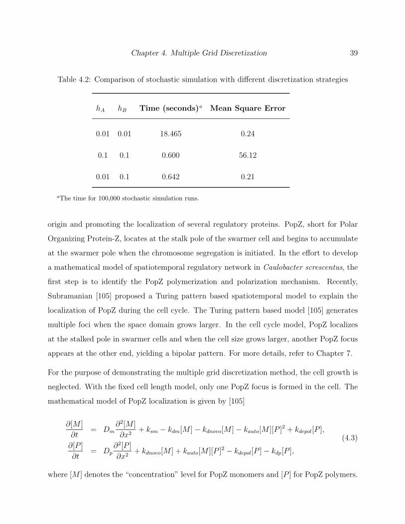
Chapter 4. Multiple Grid Discretization 39
Table 4.2: Comparison of stochastic simulation with different discretization strategies
hA hB Time (seconds)a Mean Square Error
0.01 0.01 18.465 0.24
0.1 0.1 0.600 56.12
0.01 0.1 0.642 0.21
aThe time for 100,000 stochastic simulation runs.
origin and promoting the localization of several regulatory proteins. PopZ, short for Polar
Organizing Protein-Z, locates at the stalk pole of the swarmer cell and begins to accumulate
at the swarmer pole when the chromosome segregation is initiated. In the effort to develop
a mathematical model of spatiotemporal regulatory network in Caulobacter screscentus, the
first step is to identify the PopZ polymerization and polarization mechanism. Recently,
Subramanian [105] proposed a Turing pattern based spatiotemporal model to explain the
localization of PopZ during the cell cycle. The Turing pattern based model [105] generates
multiple foci when the space domain grows larger. In the cell cycle model, PopZ localizes
at the stalked pole in swarmer cells and when the cell size grows larger, another PopZ focus
appears at the other end, yielding a bipolar pattern. For more details, refer to Chapter 7.
For the purpose of demonstrating the multiple grid discretization method, the cell growth is
neglected. With the fixed cell length model, only one PopZ focus is formed in the cell. The
mathematical model of PopZ localization is given by [105]
∂[M ]
∂t= Dm
∂2[M ]
∂x2+ ksm − kdm[M ]− kdnovo[M ]− kauto[M ][P ]2 + kdepol[P ],
∂[P ]
∂t= Dp
∂2[P ]
∂x2+ kdnovo[M ] + kauto[M ][P ]2 − kdepol[P ]− kdp[P ],
(4.3)
where [M ] denotes the “concentration” level for PopZ monomers and [P ] for PopZ polymers.

40
Table 4.3: Parameters of PopZ localization model. The parameter unit is estimated in
population number.
parameter value parameter value
Dm 250 Dp 0.01
ksm 160 kdm 0.25
kdnovo 350 kauto 0.00024
kdepol 1.0 kdp 0.075
Table 4.3 lists the parameter values for Subramanian’s PopZ polarization model, scaled
for each compartment. Figure 4.3 shows the deterministic result of the spatiotemporal
model (4.3) of fixed cell length. Colors in the map indicate population levels, where red
color means a high population level while blue denotes a low population level. Given a biased
initial condition where a small induction is initiated in the right end, the deterministic model
shows a strip at the right end of the domain.
From the deterministic model (4.3), a stochastic model of only simple chemical reactions
is built up. With the multiple grid discretization (MGD) method, the spatial domain is
partitioned into compartments of size hm for PopZ monomers and hp for PopZ polymers. In
each compartment, the reaction channels and propensity functions are given in Figure 4.4,
where mi denotes the population of PopZ monomers in the i-th compartment and pj for the
population of PopZ polymers in the j-th compartment.
The efficient discretization sizes are calculated with Formula (3.11). Because of the spatially
different populations of species P, it is tempting to use different discretization sizes at different
positions along the one dimensional domain. To simplify the simulation, spatially uniform
discretization is applied for each species. The efficient discretization sizes are calculated

Chapter 4. Multiple Grid Discretization 41
0.2 0.4 0.6 0.8 10
50
100
150
200
250
position x
t
0
10
20
30
40
50
60
70
Figure 4.3: The spatioltemporal population level of the deterministic model (4.3). Colors
indicate population level, where red color means high population while blue denotes low
population level.
using the largest population at the PopZ focus to keep the simulation accuracy. Based
on the reaction rate constants and diffusion constants, the efficient discretization sizes for
species M and P are given in table 4.4.
Figure 4.5 shows the typical stochastic simulation result of the space-discrete PopZ model
in Figure 4.4. It is interesting to see that the stochastic simulation results show two types of
PopZ population focus. Stochastic effect leads to the unbiased PopZ polarization location
no matter where the initial induction stays at the beginning.
Figure 4.6 shows the number of firings of chemical reactions and diffusive jumps during the
250 minutes model time. The number of firings of the diffusive transition is significantly
reduced with a larger discretization size, with great efficiency improvement. Table 4.5 lists
the detailed firing numbers of each reaction and diffusive jump, as well as the total simulation
time for each simulation run with different discretization strategies.
The statistics in Table 4.5 shows that the multiple grid discretization method with efficient

42
i∅ −→ Mi, a1 = ksmhm,
Mi −→ ∅, a2 = kdmmi,
Mi −→ Mi+1, a3 =Dm
h2m
mi,
Mi −→ Mi−1, a4 =Dm
h2m
mi,
Mi −→ Pj, a5 = kdnovomi,
Mi + 2 Pj −→ 3 Pj, a6 =kautohmhp
mip2j ,
Pj −→ Mi, a7 = kdepolpj,
Pj −→ ∅, a8 = kdppj,
Pj −→ Pj+1, a9 =Dp
h2p
pj,
Pj −→ Pj−1, a10 =Dp
h2p
pj,
Figure 4.4: The stochastic reaction model and the reaction propensities for the PopZ local-
ization in a single compartment i.
discretization sizes reduces the stochastic simulation time greatly. Larger discretization sizes
lead to smaller diffusion propensities, which further shorten the simulation time.
4.3 Discussion & Conclusion
A novel multiple grid discretization method for efficient stochastic simulation of multiscale
reaction diffusion systems is introduced in this chapter. With the multiple grid discretiza-
tion method, each species is assigned an efficient discretization size, which reduces diffusive

Chapter 4. Multiple Grid Discretization 43
Table 4.4: The efficient discretization sizes for PopZ monomers and polymers
KL divergence 5% 1%
M 0.07 0.03
P 0.04 0.02
10 20 30 40 50 60 70 80 90 100
50
100
150
200
250
bin No.
tim
e t
the population evolution in each bin
0
10
20
30
40
50
60
70
80
90
100
10 20 30 40 50 60 70 80 90 100
50
100
150
200
250
bin No.
tim
e t
the population evolution in each bin
0
10
20
30
40
50
60
70
80
90
100
Figure 4.5: The spatiotemporal population evolution of PopZ polymer in the stochastic
simulation. The stochastic simulation results demonstrate that PopZ focus polarizes in
either end of the cell.
transitions between neighboring compartments. Decreasing of diffusive jumps greatly im-
proves the simulation efficiency over the traditional RDME method. Though this chapter
is discussed with reaction-diffusion models in one dimensional space, the adaption to two
dimensional models and three dimensional models is rather straightforward.
The multiple grid discretization method focuses on the simulation efficiency improvement
with error-controllable discretization sizes. Further investigation on compartment-based Tur-
ing model simulations shows that multiple grid discretization method changes the parameter
regime for pattern formation [11]. It is discovered that the parameter regimes of MGD for

44
Table 4.5: Firing numbers of reaction/diffusion events and simulation CPU time for different
discretization strategies
Discretization Size
M size 0.01 0.04 0.07 0.20
P size 0.01 0.02 0.03 0.05
null→ M 4.0E4 (0.0%) 4.0E4 (0.0%) 4.0E4 (0.1%) 4.0E4 (0.5%)
M→ null 7.1E1 (0.0%) 7.2E1 (0.0%) 7.2E1 (0.0%) 7.2E1 (0.0%)
Mi → Mi+1 7.1E8 (46.7%) 4.4E7 (38.7%) 1.5E7 (38.0%) 1.4E6 (18.7%)
Mi → Mi−1 7.1E8 (46.7%) 4.4E7 (38.7%) 1.5E7 (38.0%) 1.4E6 (18.8%)
M→ P 1.0E5 (0.0%) 1.0E5 (0.1%) 1.0E5 (0.3%) 1.0E5 (1.3%)
M + 2 P→ 3 P 4.4E5 (0.0%) 4.4E5 (0.4%) 4.4E5 (1.1%) 4.5E5 (5.8%)
P→ M 5.0E5 (0.0%) 5.0E5 (0.4%) 5.0E5 (1.3%) 5.0E5 (6.6%)
P→ null 3.8E4 (0.0%) 3.8E4 (0.0%) 3.8E4 (0.1%) 3.8E4 (0.5%)
Pi → Pi+1 5.0E7 (3.2%) 1.2E7 (10.8%) 4.3E6 (10.6%) 1.8E6 (24.1%)
Pi → Pi−1 5.0E7 (3.2%) 1.2E7 (10.7%) 4.3E6 (10.5%) 1.8E6 (23.7%)
CPU time (seconds) 1551.4 61.2 18.4 4.2

Chapter 4. Multiple Grid Discretization 45
1 2 3 4 5 6 7 8 9 100
1
2
3
4
5
6
7
8x 10
8
reaction No.
firings
The firings of each reaction with Mmesh = Pmesh = 0.01
1 2 3 4 5 6 7 8 9 100
2
4
6
8
10
12
14
16
18x 10
6
reaction No.
firings
Firings of each reaction with optimal mesh size of 5% KL divergence
Figure 4.6: The firings of reaction and diffusion events with different discretization strategies.
Left: uniform discretization with discretization size h = 0.01 for both species M and P. Right:
multiple grid discretization with the efficient discretization sizes of 5% relative error. It is
apparent that the firing number of the diffusive jumps significantly decreases.
pattern formation is different from the parameter regimes of the deterministic PDE model,
also different from the parameter regimes of the regular uniform discretization method. This
discovery signals a warning against the further simulation of the Turing based model with
multiple grid discretization method.

Chapter 5
The Hill Function Dynamics in
Reaction-Diffusion Systems
In addition to simple mass law reaction rates, many highly nonlinear phenomenological
reaction rate laws have been used in mathematical modeling of biological systems. For
example, the Michaelis-Menten and Hill functions are widely used in biological models to
model fast responses to signals in regulatory control. Most of the time, theoretical biologists
are not interested in the detailed mechanisms behind these phenomenological reaction rate
laws, either because the detailed mechanisms are not clear or not important.
The stochastic simulation of Caulobacter crescentus reveals a misbehavior of Hill function
dynamics in reaction-diffusion systems. Numerical analysis with a toy reaction-diffusion
gene regulation model in Section 5.3 shows that when discretization sizes are small enough,
the switch behavior of Hill dynamics becomes a linear function of the input signal and
the discretization size. Section 5.4 provides a remedy for the discretization of reaction-
diffusion systems with Hill function rate laws. The numerical analysis and experiment results
demonstrate Hill function dynamics in reaction-diffusion systems lead to convergent results
only if signaling species have impact within a fixed length domain, rather than just within
the same RDME compartment. This fixed length is referred to as the Hill function reaction
46

Chapter 5. The Hill Function Dynamics in Reaction-Diffusion Systems 47
radius, a critical signaling distance threshold below which the system breaks down. Finally,
this chapter is concluded with an assessment of nonlinear dynamics in RMDE and future
development.
5.1 Hill Function Dynamics in Reaction-Diffusion Sys-
tems
The Hill function, as well as the Michaelis-Menten function, is widely used in modeling
of enzyme kinetics. In molecular biology, enzymes catalyse the conversion of biochemical
substrates into products, while remaining basically unchanged. The enzyme kinetics reaction
is usually described as
E + Sk1−−−−k−1
ESk2−→ E + P. (5.1)
With the conservation law and the “quasi-steady state” assumption, the enzyme kinetics
reaction rate function, referred to as the Michaelis-Menten function, is formulated as
d[P ]
dt= Vmax
[S]
KM + [S], (5.2)
with Vmax = k2[E]0 the maximum reaction rate and Km = k−1+k2k1
the Michaelis constant.
In gene regulation models, several transcription factor (TF) molecules often bind with a
piece of DNA promoter sequence and control the gene expression. The binding reaction can
be simply expressed as
DNA + nTFk1−−−−k−1
DNA− nTFk2−→ gene expression. (5.3)
In realistic biological models, the binding of the n transcription factor molecules to DNA
does not take place all at once but rather in a succession of steps. Using the equilibrium
assumption and conservation laws, the reaction equation of the transcription factor regulated
DNA expression can be written as
d[P ]
dt= Vmax
[TF ]n
Kmn + [TF ]n
, (5.4)

48
with Vmax the maximum reaction rate, Km the Michaelis constant and n the Hill coefficient.
5.2 Caulobacter Cell Cycle Modeling
Caulobacter crescentus attracts interest as an example of asymmetric cell division. When a
Caulobacter cell divides, it produces two functionally and morphologically distinct daughter
cells. The asymmetric cell division of Caulobacter crescentus requires elaborate temporal
and spatial regulations [66, 67, 104, 106].
CtrA, one of the four essential “master regulators” of the Caulobacter cell cycle [17, 18,
48], oscillates temporally and spatially and drives a series of modular functions during the
cell cycle. In swarmer cells, CtrA is phosphorylated by a two-component phosphorelay
system (CckA and ChpT). Phosphorylated CtrA (CtrAp) binds to the chromosomal origin
of replication (Cori) and inhibits the initiation of chromosome replication [91]. During
the swarmer-to-stalked transition, CtrAp gets dephosphorylated and degraded, allowing the
initiation of chromosome replication. For more details, refer to Chapter 6.
In order to study the regulatory network in Caulobacter crescentus, a deterministic model
with six major regulatory proteins is developed [104, 106]. The deterministic model provides
robust switching between swarmer and stalked states. Figure 5.1 (left) demonstrates the
total population change during the Caulobacter crescentus cell cycle with this deterministic
model. In the swarmer stage (t = 0 − 30 min), the CtrA is phosphorylated at a high
population level, which inhibits the initiation of chromosome replication. During swarmer-
to-stalk transition (t = 30 − 50 min), the CtrAp population quickly drops to a low level,
allowing the consequent initiation of chromosome replication in the stalked stage.
In stochastic simulation of the spatiotemporal model of this regulatory network, the phos-
phorylated CtrA (CtrAp) population switch from high in swarmer stage to low in stalked
stage is not as sharp as expected, shown in Figure 5.1 (right). On the other hand, the DivL
population level from the stochastic simulation seems similar to that from the deterministic

Chapter 5. The Hill Function Dynamics in Reaction-Diffusion Systems 49
simulation. A simple analysis suggests the Hill function dynamics, which model the up reg-
ulation of CckA kinase activity by DivL, might be the culprit. Further investigation leads to
the discovery of the Hill function limitation at fine discretizations, as analyzed in the next
section.
0 20 40 60 80 100 1200
20
40
60
80
100
120
time min
po
pu
lati
on
DivLCckA kinCtrAp
0 20 40 60 80 100 1200
20
40
60
80
100
120
time min
popula
tion
DivLCckA kinCtrAp
Figure 5.1: The population oscillation of CtrAp during the Caulobacter crescentus cell cycle.
The left figure shows the deterministic model simulation result and the right figure shows
the stochastic model simulation result. In the swarmer stage (t = 0− 30 min), the CtrA is
phosphorylated and at a high population level, which inhibits the initiation of chromosome
replication. During swarmer-to-stalk transition (t = 30 − 50 min), the CtrAp population
quickly switches to a low level, allowing the consequent initiation of chromosome replication
in the stalked stage.
5.3 Hill Function Dynamics in Reaction-Diffusion Sys-
tems
To simplify the analysis, a toy gene regulation model of a reaction-diffusion system in one
dimension is constructed. As demonstrated in figure 5.2, in the toy model, a transcription
factor (TF) is constantly synthesized and degraded. The transcription factor (TF) further

50
Figure 5.2: A simple gene regulation model of Hill function dynamics in one dimensional
domain. Transcription factor (TF) is constantly synthesized and upregulates the DNA ex-
pression.
upregulates the DNA expression.
Assume the spatial domain of size L is equally partitioned into K compartments with size h =
L/K. The chemical reactions and reaction propensities in each compartment are formulated
as
∅ → TFi, a1 = ks · h,
TFi → ∅, a2 = kd · Ei,
∅ TFi−−→ mRNAi, a3 = ksyn · hE4i
(Km · h)4 + E4i
,
mRNAi → ∅, a4 = kdeg · Pi,
TFi → TFi±1, a5 = 2Dtf
h2Ei,
mRNAi → mRNAi±1, a6 = 2Drna
h2Pi,
(5.5)
where Ei denotes the population of transcription factor TF and Pi denotes the population of
mRNA in the ith compartment. The parameters ks, kd are the synthesis, degradation rates,
respectively, for transcription factor, and similarly ksyn, kdeg are those for mRNA synthesis.
Km is the Michaelis constant in the Hill function.
In the one-dimensional domain, the transcription factor is constantly synthesized and de-
graded. At the equilibrium state, the distribution of the total population of transcription

Chapter 5. The Hill Function Dynamics in Reaction-Diffusion Systems 51
factor is estimated by the Poisson distribution (see Appendix A for details),
PE(n) ≈ αn
n!e−α, (5.6)
where α = kskdL denotes the mean of the total number of mRNA molecules in the domain.
For an individual compartment (bin), consider the probability P(i)E (n) that an individual bin
i contains n molecules of transcription factor. At the equilibrium state, transcription factor
is homogeneously distributed in the system. The probability that each molecule of TF stays
in a certain bin i is given by p = 1/K. The probability that, of all the TF molecules in the
domain, none is in bin i is approximated by
P(i)E (0) = PE(0) + PE(1)
(1− 1
K
)+ PE(2)
(1− 1
K
)2+ . . .+ PE(N)
(1− 1
K
)N≈
N∑n=0
e−ααn
n!
(1− 1
K
)n≈ e−α/K .
(5.7)
The other probability terms are not important in the analysis.
With the distribution of the TF molecular population, the mean reaction propensity for the
synthesis of mRNA in the ith bin is
〈a(i)syn〉 = ksynh
N∑n=0
n4
(Km · h)4 + n4P
(i)E (n). (5.8)
Notice that when n = 0, the Hill function is zero, and when the discrete bin size h is small,
the Hill function approaches one quickly as n → ∞. For example, when Km · h ≤ 0.5 the
Hill function n4
(Km·h)4+n4 ≥ 0.94 for n ≥ 1. Therefore, upper and lower bounds for the mRNA
synthesis propensity, when km · h ≤ 0.5, are
0.94ksynhN∑n=1
P(i)E (n) ≤ 〈a(i)
syn〉 ≤ ksynhN∑n=1
P(i)E (n). (5.9)
Hence, when the discretization size h is small enough, the propensity for the mRNA synthesis

52
reaction can be approximated as
〈a(i)syn〉 ≈ ksynh
N∑n=1
P(i)E (n)
= ksynh(1− P (i)E (0))
≈ ksynh(1− e−α/K).
(5.10)
When the discretization size is small and K is large, the mean reaction propensity can be
further approximated as
〈a(i)syn〉 ≈ ksyn · h · α/K. (5.11)
Notice that α/K is the mean population of TF in ith bin. The Hill dynamics of the mRNA
synthesis is now reduced to a linear function of the TF population in ith bin.
Furthermore, from (5.11) the mean population of mRNA in the bin i is
〈P (i)〉 ≈ ksyn · hkdeg
α
K, (5.12)
and the total mRNA population in all K bins is
〈P 〉 ≈ ksyn · Lkdeg
ks · Lkd
1
K
=ksynkdeg· α · h.
(5.13)
Equation (5.13) shows that the total population of mRNA is a linear function of the mean
population of TF α and the discretization size h = L/K. With finer discretization, less
mRNA is produced. Figure 5.3 shows the histogram and the mean value of the mRNA pop-
ulation with different discretization sizes. The histograms show that with finer discretization,
the population histograms shift further to the left.
The log-log plot shows that when the discretization size is small enough, the total mRNA
population is a linear function of discretization size. The slope of the log-log plot is about
1.0 at small discretization size h. Moreover, the simulation result shows that when the mean

Chapter 5. The Hill Function Dynamics in Reaction-Diffusion Systems 53
TF population is less than the constant Km in the Hill function (Km > α), the population of
mRNA P increases slightly before the Hill function dynamics breaks at small discretization
sizes. Note that the Hill function dynamics show a concave shape with respect to TF
population when the TF population is smaller than the Michaelis constant Km. Therefore,
it is reasonable that the mRNA population in this reaction-diffusion model increases slightly
when the Michaelis constant Km is larger than the mean TF population α.
0 10 20 30 40 50 60 70 800
0.02
0.04
0.06
0.08
0.1
0.12
0.14
0.16
0.18
0.2
population
pro
ba
bil
ity
h = 0.002
h = 0.005
h = 0.01
h = 0.02
h = 0.05
10−3
10−2
10−1
100
101
102
h
me
an
po
pu
latio
n
Km
= 10
Km
= 25
Km
= 50
Figure 5.3: The histogram (left) and mean (right) population of mRNA with different dis-
cretizations. Parameters: De = 1.0, ks = 2.5, kd = 0.1, ksyn = 5.0, kdeg = 0.05, system
size L = 1.0. For the histogram figure, Km = 25.0. The log-log plot shows the mean total
mRNA population under different discretizations and different parameter values.
To get the linear relation, the numerical analysis above makes two approximationsn4
(Km · h)4 + n4≈ 1, for n ≥ 1,
e−α/K ≈ 1− α/K.(5.14)
Assuming an error tolerance of 5%, the two approximations can be simplified toKm · h < 0.5,
α/K < 1/3.
(5.15)
Hence, when the discretization bin number
K > max2LKm, 3α, (5.16)

54
the Hill dynamics reduce to a linear function.
Equivalently, in order for the Hill function dynamics to work well, the discretization number
K should be less than or equal to this threshold. However, the coarse discretization from
a small K leads to spatial error. Two potential solutions to this discretization dilemma are
proposed next.
5.4 Convergent Hill Function Dynamics with RDME
From the previous analysis, the Hill dynamics in RDME systems fail due to the lack of
intermediate states — the discrete population in each individual bin yields a constant value
(0 or 1) for the Hill function. An intermediate state is generated by a smoothing technique
that averages the population over neighboring bins when calculating the reaction propensity.
To model a RDME system in high dimensions with fine discretization, many studies have
suggested relaxing the same-compartment reaction assumption and allowing the reactions
within neighboring compartments. A natural technique that bridges the discrete and contin-
uous models is to smooth the spatial population by taking the average of neighboring bins.
Consider first smoothing the TF population within the neighboring m bins (including the
bin itself) when calculating the reaction propensity.
Following Section 5.3, the reaction probability for the synthesis of mRNA in the ith bin is
〈a(i)syn〉 = ksyn · h
N∑n=0
( (n/m)4
(Km · h)4 + (n/m)4P
(i)E (n;m)
)= ksyn · h
N∑n=0
( n4
(m ·Km · h)4 + n4P
(i)E (n;m)
),
(5.17)
where P(i)E (n;m) denotes the probability that the m neighboring bins of the ith bin have a
total TF population of n. The interpretation of this equation is that the synthesis reaction
in the ith bin is interacting with the m neighboring bins and the propensity is calculated

Chapter 5. The Hill Function Dynamics in Reaction-Diffusion Systems 55
based on the total TF population of all the neighboring bins. By probability theory,
P(i)E (0;m) ≈ e−αm/K . (5.18)
As before, only the term P(i)E (0;m) is important.
In Equation (5.17), for any fixed integer m ≥ 0, there exists h ≥ 0, such that m ·Km ·h < 0.5
and the Hill function is approximately one. At such a discretization size h, the mRNA
synthesis propensity can be approximated as
〈a(i)syn〉 ≈ ksyn · h
N∑n=1
P(i)E (n;m)
= ksyn · h(1− P (i)E (0;m))
≈ ksyn · h(1− e−αm/K)
≈ ksyn · h · α ·m/K.
(5.19)
Again, with a fixed smoothing bin number m, the synthesis reaction propensity becomes
linear in the mean TF population αm/K of the m bins, and the mean population of mRNA
P in the system is
〈P 〉 =ksyn · Lkdeg
ks · Lkd
m
K, (5.20)
which is linear in m/K and the mean total TF population α. The linear relation obtains
with h such that m ·Km · h < 0.5,
m · α/K < 0.33.
(5.21)
Figure 5.4 plots the mean population of mRNA in the toy model with the smoothing tech-
nique and m = 5. The experimental results show that smoothing over a fixed number m
of compartments gives a good solution for a certain range of discretization sizes. However,
there always exists a small enough discretization size h such that the Hill function dynamics
reduce to a linear function with respect to the discretization size. Moreover, fixed length
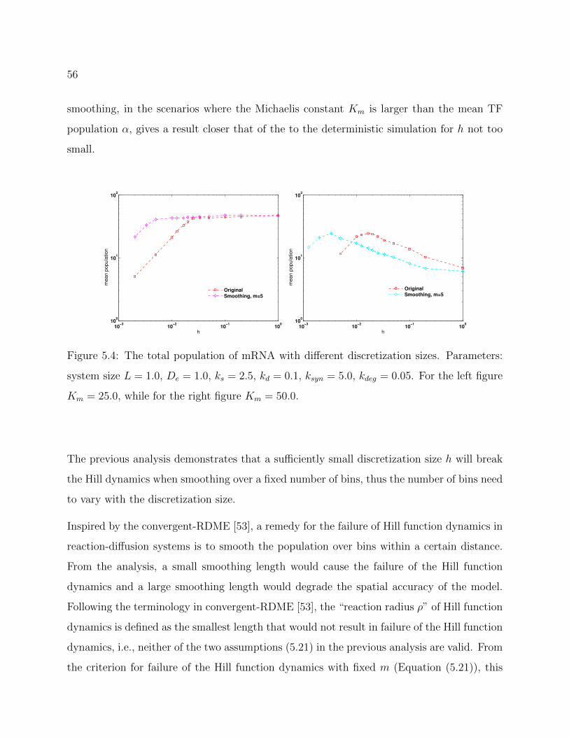
56
smoothing, in the scenarios where the Michaelis constant Km is larger than the mean TF
population α, gives a result closer that of the to the deterministic simulation for h not too
small.
10−3
10−2
10−1
100
100
101
102
h
mean p
opula
tion
OriginalSmoothing, m=5
10−3
10−2
10−1
100
100
101
102
h
mean p
opula
tion
OriginalSmoothing, m=5
Figure 5.4: The total population of mRNA with different discretization sizes. Parameters:
system size L = 1.0, De = 1.0, ks = 2.5, kd = 0.1, ksyn = 5.0, kdeg = 0.05. For the left figure
Km = 25.0, while for the right figure Km = 50.0.
The previous analysis demonstrates that a sufficiently small discretization size h will break
the Hill dynamics when smoothing over a fixed number of bins, thus the number of bins need
to vary with the discretization size.
Inspired by the convergent-RDME [53], a remedy for the failure of Hill function dynamics in
reaction-diffusion systems is to smooth the population over bins within a certain distance.
From the analysis, a small smoothing length would cause the failure of the Hill function
dynamics and a large smoothing length would degrade the spatial accuracy of the model.
Following the terminology in convergent-RDME [53], the “reaction radius ρ” of Hill function
dynamics is defined as the smallest length that would not result in failure of the Hill function
dynamics, i.e., neither of the two assumptions (5.21) in the previous analysis are valid. From
the criterion for failure of the Hill function dynamics with fixed m (Equation (5.21)), this

Chapter 5. The Hill Function Dynamics in Reaction-Diffusion Systems 57
choice is
ρ = mh
= max
1
2Km
,L
3α
= max
1
2Km
,1
3ks/kd
.
(5.22)
Equation (5.22) shows the Hill function reaction radius of a reaction-diffusion system is a
constant, defined by the chemical reaction rate constants only.
For any discretization size h, the number of compartments to be smoothed over is given by
m = dρhe. (5.23)
Figure 5.5 shows the results for the toy gene regulation model in the reaction-diffusion system
with different discretization sizes and with the convergent smoothing technique (m and h
related by (5.23)).
10−3
10−2
10−1
100
100
101
102
h
mean p
opula
tion
Original
Smoothing, m=5
Fixed Length Smoothing
10−3
10−2
10−1
100
100
101
102
h
mean p
opula
tion
Original
Smoothing, m=5
Fixed Length Smoothing
Figure 5.5: The histogram and the mean population of mRNA with different discretization
sizes. Parameters: system size L = 1.0, De = 1.0, ks = 0.025, kd = 0.1, ksyn = 0.05,
kdeg = 0.05. For the left figure Km = 25.0, while for the right figure Km = 50.0.

58
5.5 Conclusions
Motivated by the misbehavior of DivL-CckA dynamics during the stochastic simulation of
the Caulobacter crescentus cell cycle, an investigation of Hill function dynamics in reaction-
diffusion systems reveals that when the discretization size is small enough, the switch-like
behavior of Hill function dynamics reduces to bimolecular reaction dynamics. A proposed
fixed length smoothing method allows chemical reactions to occur with the reactant molecules
within a distance of fixed length, the “reaction radius”of the Hill function dynamics.
Applying the fixed length smoothing technique to the DivL-CckA Hill function model in
the Caulobacter crescentus cell cycle results in a sharp CtrAp population change during
swarmer-to-stalk transition. Figure 5.6 shows the CtrAp trajectories from the deterministic
model and stochastic model simulation results. The fixed length smoothing technique yields
more CtrAp in the swarmer stage and less CtrAp in the stalked stage, which yields a sharp
CtrAp population change during the swarmer-stalk transition as expected.
0 20 40 60 80 100 1200
20
40
60
80
100
120
time min
po
pu
lati
on
deterministicoriginalSmoothing
5 20 35 50 65 80 95 110 125 140 155 170 185 2000
0.05
0.1
0.15
0.2
0.25
0.3
0.35
0.4
CtrAp population
pro
ba
bili
ty
Original
Smoothing
Deterministic
Figure 5.6: The comparison of CtrAp from the deterministic model and the stochastic model
simulation results. Left: CtrAp population trajectory during Caulobacter crescentus cell
cycle. Right: The histogram of the CtrAp population in swarmer cells (t = 30 min). For
model parameters, refer to Chapter 6.
It is known that in high dimensions bimolecular reactions are lost with the RDME in
the microscopic limit [52]. This work shows one-dimensional Hill function dynamics in a

Chapter 5. The Hill Function Dynamics in Reaction-Diffusion Systems 59
RDME framework reduce to simple bimolecular dynamics when the discretization size is
small enough. The conjecture is that the problem lies in the RDME requirement that the
reactions only fire with the reactant molecules in the same discrete compartment. Further-
more, this defect in RDME at the microscopic limit is believed to be a common scenario for
all highly nonlinear reaction dynamics. Theoretical biologists have developed many highly
nonlinear reaction dynamics that need special attention when converted to stochastic mod-
els. Future work will continue the investigation of stochastic modeling and simulation of
highly nonlinear reaction dynamics in the RDME framework, including higher dimensions.
Chapter 6
Stochastic Spatiotemporal Model of
Response-Regulator Network in the
Caulobacter crescentus Cell Cycle
The asymmetric cell division cycle in Caulobacter crescentus is controlled by an elaborate
molecular mechanism governing the production, activation and spatial localization of a host
of interacting proteins. In previous studies, Subramanian proposed a deterministic mathe-
matical model for the spatiotemporal dynamics of six major regulatory proteins. A stochastic
version of Subramanian’s model, which takes into account molecular fluctuations of the regu-
latory proteins in space and time during early stages of the cell cycle of wild-type Caulobacter
cells, is presented in this chapter. The stochastic model demonstrates the increased variabil-
ity of cycle time in cells depleted of the divJ gene product, which is observed in single-cell
experiments. The deterministic model predicts that overexpression of the divK gene blocks
cell cycle progression in the stalked stage; however, stochastic simulations suggest that a
small fraction of the mutants cells do complete the cell cycle normally.
60

Chapter 6. Histidine Kinase Switch Model in Caulobacter crescentus 61
6.1 Background
Stalk formation
Flagelum
assembly
Pili
synthesis
Flagellum shedding
Pili retraction
Predivisional
cell
Swarmer
cell
Stalked
cell
S
G2
G1
Figure 6.1: The asymmetric division cycle of Caulobacter cells.
Caulobacter crescentus is an aquatic α-proteobacterium that is widely distributed in fresh-
water lakes and streams [63]. As illustrated in Figure 6.1, Caulobacter cells divide asymmet-
rically [19, 9, 89, 98]. The larger cell, called the stalked cell, is anchored to its substratum by
a stalk and holdfast. The stalked cell is able to initiate chromosome replication and begin
the division-differentiation cycle immediately. The smaller cell, called the swarmer cell, is
equipped with a polar flagellum and several pili, with which it swims away from its place
of birth. The swarmer cell is not competent for chromosome replication and cell division
until it differentiates into a stalked cell. The swarmer-to-stalked transition involves shedding
the flagellum, retracting the pili, and constructing a stalk in their place. The stalked cell
grows primarily in length (slightly banana-shaped) and eventually builds a flagellum at the
“new” pole (the pole derived from the septum at the previous division). After chromosome
replication and segregation is completed, a ring of tubulin-like proteins (FtsZ) constricts and
divides the cytoplasm into two separate compartments [56]. Cytoplasmic compartmental-
ization enables divergent programs of cell differentiation, yielding two distinct progeny: a

62
stalked cell and a swarmer cell.
Asymmetric cell division is a common feature of cell proliferation in many types of or-
ganisms [103, 81, 87, 88, 115, 21]. Typical of these situations, the asymmetric division-
differentiation cycle of Caulobacter crescentus involves an elaborate sequence of spatiotem-
porally regulated protein interactions that control chromosome segregation, polar differen-
tiation and regulator localization [62, 3]. Experimentalists have identified four essential
“master regulators” of the Caulobacter cell cycle, namely DnaA, GcrA, CtrA and CcrM,
which determine the temporal expression of approximately 200 genes [17, 18, 48]. These
master transcription regulators oscillate temporally and spatially and drive a series of mod-
ular functions during the cell cycle. The molecular mechanisms governing CtrA functions
have been studied in great detail, but the controls of DnaA, GcrA and CcrM are less well
known.
In swarmer cells, CtrA is phosphorylated by a two-component phosphorelay system (CckA
and ChpT). Phosphorylated CtrA (CtrAp) binds to the chromosomal origin of replication
(Cori) and inhibits the initiation of chromosome replication [91]. During the swarmer-to-
stalked transition, CtrAp gets dephosphorylated and degraded, allowing the initiation of
chromosome replication. CtrA is degraded by an ATP-dependent protease, ClpXP [76, 54],
which is localized to the stalk pole by the unphosphorylated response regulator CpdR. As
the nascent stalked cell progresses through the replication-divison cycle, CpdR is phospho-
rylated by CckA-ChpT, loses it polar localization, and, consequently, loses its ability to
recruit ClpXP protease for CtrA degradation. In addition, CckA-ChpT phosphorylate and
reactivate CtrA [51]. Although the mechanisms connecting CckA to CtrA functions have
been identified, the pathways for CckA localization and regulation are still unclear.
Development of the flagellated pole is controlled by the phosphorylation state of DivK in
response to the histidine kinase DivJ and the bifunctional histidine kinase/phosphatase
PleC [50]. The DivJ-PleC-DivK pathway regulates the phosphorylation status of PleD,
which governs polar development, such as flagellum shedding and stalk biosynthesis. At the

Chapter 6. Histidine Kinase Switch Model in Caulobacter crescentus 63
swarmer-to-stalked transition, PleD is phosphorylated by PleC kinase and localized at the
stalk pole. Localized PleD induces the synthesis of the second messenger, cyclic di-GMP, to
signal stalk development. The non-canonical histidine kinase, DivL [110], promotes CckA
kinase activity. CckA kinase phosphorylates and activates CtrA in the swarmer cell. In the
stalked cell, phosphorylated DivK binds to DivL and inhibits CckA kinase activity. During
the swarmer-to-stalked transition, DivJ phosphorylates DivK. Phosphorylated DivK in turn
binds and inhibits DivL, thereby inhibiting CckA kinase activity. Subsequent dephosphory-
lation and degradation of CtrA allows the initiation of chromosome replication.
As the cell progresses into the previsional stage, PleC accumulates at the new pole. While
the bifunctionality of CckA as a phosphatase and kinase is well known, the potential bi-
functionality of PleC as a histidine phosphatase/kinase in predivisional cells has been under
debate for some time [106]. Experiments [85, 1] show that phosphorylated DivK (DivKp)
up-regulates the kinase form of PleC. By phosphorylating PleD, PleC kinase initiates the
pathway for stalk pole development. This view of PleC as a kinase at the old pole raises a
question of what is happening at the new pole of predivisional cells (the nascent swarmer
pole). The canonical view [110, 73] suggests that in the predivisional cell PleC functions as
a phosphatase at the new pole, where it dephosphorylates DivK and creates a protection
zone for active DivL, active CckA, and CtrA phosphorylation. An alternate view is that
PleC remains a kinase in previsional cells. However, this raises the question of how DivL
is protected form the inhibitory effect of DivKp. Recently, using a mathematical model
(reaction-diffusion equations) of the DivJ-PleC-DivK and DivL-CckA-CtrA network, Subra-
manian et al. [106] provide support for the view that PleC is a kinase at the new pole. Their
simulations show that PleC kinase at the new pole of a predivisional cell can sequester DivKp
from binding to DivL. Free DivL upregulates CckA, thereby promoting phosphorylation of
CtrA and the formation of CtrAp gradient in the predivisional cell. After constriction of the
FtsZ ring, compartmentalization of the predivisional cell separates PleC kinase at the new
pole from DivJ kinase at the old pole. PleC reverts back to a phosphatase. As a consequence,
DivK is dephosphorylated in the swarmer cell compartment, while phosphorylated DivK is

64
retained in the stalked cell compartment.
Although cell cycle progression in Caulobacter is robust in respect to protein regulation and
the proper sequence of events, cells exhibit considerable variability in other respects, such
as the times spent in various phases of the cycle and the sizes of cells at the time events
occur [68]. These variabilities in cell cycle progression are attributable in large part to
the fact that the populations of protein species in a single Caulobacter cell are limited in
number and therefore subject to random molecular fluctuations. For example, the volume
of a Caulobacter cell is roughly 1 fL ∗ at division and contains around 300 molecules of a
particular protein species (if its concentration is around 500 nmol/L). Moreover, the number
of mRNA molecules for each protein at any time is likely to be around 10 [107]. With such
numbers of mRNAs and proteins, molecular fluctuations at the protein level are expected to
be ∼ 25% [86]. Such large fluctuations in protein levels may significantly affect the properties
of the cell cycle control system. For example, recent optical microscopy measurements reveal
an intriguing role of DivJ in the control of noise in single Caulobacter cells [100]: the data
show that depleting cells of DivJ causes (in addition to a modest increase of ∼ 16 min in
mean interdivision time) a large increase in the variance of interdivision times (the coefficient
of variation of interdivision times increases from ∼ 11% for wild-type cells to ∼ 26% for divJ-
deleted cells).
Recently, Lin et al. [68], propose a simplified protein interaction network that captures the
noisy oscillations of protein abundances during the Caulobacter cell cycle and accounts for
the observations of the variability of cell cycle periods in wild-type and divJ-deleted cells. Lin
et al.’s model is illuminating, but it suffers some shortcomings: it does not take into account
the effects of fluctuations at the mRNA level or of the spatial distributions of the regulatory
proteins, and it relies on a “non-detailed” simulation of stochastic processes. In this chapter,
a stochastic model avoiding theses shortcomings is developed, by extending the determinis-
tic reaction-diffusion model of Subramanian et al. [106] to a mechanistically detailed, spa-
∗femto- (f) is a unit prefix in the metric system denoting a factor of 10−15. 1 fL = 10−15 L.

Chapter 6. Histidine Kinase Switch Model in Caulobacter crescentus 65
tiotemporal, stochastic model, including mRNA species. Furthermore, the stochastic model
is utilized to demonstrate the effects of divJ deletion and divK overexpression on cell cycle
progression in single Caulobacter cells. Stochastic simulations of the divJ-deletion strain are
consistent with the observations of Lin et al. [68], and simulations of divK-overexpression
strains predict a stochastic phenotype of these cells: although most cells are blocked in the
stalked stage of the cell cycle (as predicted by the deterministic model of Subramanian et
al. [106]), some cells are able to complete the cell cycle normally.
6.2 Method
Figure 6.2: Regulatory network of two phosphorelay systems that play major roles in the cell
division cycle of Caulobacter crescentus. The phosphorylated form of CtrA inhibits the initiation
of chromosome replication in swarmer cells. The phosphorylated form of DivK indirectly inhibits
the phosphorylation of CtrA, through the DivL–CckA pathway. The kinase activity of the enzyme,
PleC, is up-regulated by the product, DivKp, of the kinase reaction.
Figure 6.2 shows the regulatory network of six regulatory proteins during the Caulobac-
ter cell cycle, proposed by Subramanian et al. [106]. PleC acts as a bifunctional histidine
kinase/phosphatase, catalyzing the transformations between DivK and DivKp [104]. Signif-
icantly, DivKp up-regulates the kinase activity of PleC [85]. Figure B.1 (in Appendix B)

66
shows the detailed scheme of PleC transformations between phosphatase and kinase, de-
pending on how the various forms of PleC are bound to DivK and DivKp. The activation
of CckA kinase by DivL is described by a Hill function (this is the only aspect of the model
that is not described by mass-action kinetics). CtrA is phosphorylated by CckA kinase, and
dephosphorylated by CckA phosphatase. Linkage between the DivJ-DivK-PleC and DivL-
CckA-CtrA modules is achieved by the binding of DivKp to DivL, which prevents DivL from
upregulating the kinase activity of CckA. The state of CtrA serves as the final output signal
in Subramanian’s model.
The deterministic spatiotemporal model [106] robustly captures the localization and activi-
ties of the regulatory proteins. However, it fails to capture the molecular noise intrinsic to
the reaction network. In order to study noise in protein populations and cell cycle periods, a
discrete stochastic model based on the deterministic model is developed. In addition to the
protein dynamics of the original model, the dynamics of genes (divJ, divK, divL, pleC, cckA,
ctrA) and mRNAs are also taken into account to determine how fluctuations at the level of
nucleic acids affects fluctuating protein levels during the Caulobacter cell cycle. Table B.1 (in
Appendix B) provides a complete list of reactions and propensities for the discrete stochastic
model.
As explained in “Model Details” (Section B.1 in Appendix B), the stochastic model en-
forces several discrete events on the reaction-diffusion equations governing DivJ, DivK, DivL,
PleC, CckA and CtrA. In paticular, “localization indicator functions” (see figure B.2 in Ap-
pendix B) is utilized to force DivJ, PleC, DivL and CckA molecules to become localized to
specific places in the cell in specific stages of the cell cycle, based on experimental observa-
tions on wild-type cells.
Gillespie’s stochastic simulation algorithm (SSA) [35, 36] is one of the most widely used
stochastic simulation methods for “well-stirred” biochemical systems. For reaction-diffusion
(RD) systems, the “well-stirred” assumption is no longer valid and Gillespie’s direct SSA
method cannot be directly applied. A common practice is to discretize the spatial domain

Chapter 6. Histidine Kinase Switch Model in Caulobacter crescentus 67
according to the Reaction Diffusion Master Equation (RDME) framework [32, 52]. The key
assumption of the RDME is that all species in each compartment are well-stirred. In this
case, chemical reactions in each compartment can be simulated by the SSA and diffusion can
be modeled as random walk among neighboring compartments. If the discretization size is
h, the propensity for one molecule to jump to one of its nearest neighbors is given by D/h2,
where D is the diffusion rate constant.
For Caulobacter, the banana shaped cell is modeled as a one dimensional domain along its
long axis, which is discretized into 50 compartments (“bins”), according to the RDME frame-
work. In each compartment, all chemical reactions (listed in table B.1) as well as all diffusive
jumps (listed in table B.2) are simulated by “direct method” of SSA. During cell growth,
the number of bins keeps constant, while the length of each bin increases exponentially with
time. Refer to the supplementary materials for more details about the stochastic model and
the stochastic simulation method.
6.3 Results
6.3.1 PleC Kinase Sequesters DivKp in the Early Predivisional
Stage
In the predivisional stage, active DivL at the new pole upregulates CckA kinase there, which
promotes CtrA phosphorylation at the new pole. At the old pole, DivL is lacking and CckA
is in the phosphatase form, dephosphorylating CtrA at the stalked end of the cell. These
effects create a gradient of CtrA phosphorylation from the new pole toward the old pole of
the early predivisional cell. This gradient is crucial for further asymmetric cell development.
Early in the predivisional stage, PleC becomes localized to the new pole [108].
It is unclear if PleC in the predivisional stage is a phosphatase or a kinase [108, 55] The
deterministic model [106] showed that once PleC becomes a kinase in the stalked cell, it

68
remains a kinase even in the predivisional cell. It is only after cytokinesis separates DivJ
and PleC into separate compartments that PleC reverts back to a phosphatase. This result is
counterintuitive, because PleC kinase would be expected to phosphorylate DivK and DivKp
would bind to and inhibit DivL (see Figure 6.2). However, the stochastic simulations also
showed that the DivKp is present in complex with PleC [104, 106]. Therefore, a hypothesis
is suggested that the kinase form of PleC may sequester DivKp away from DivL.
Figure B.3 shows histograms of DivKp and DivL components in the early predivisional stage
(t = 120 min). Most DivKp molecules are complexed with PleC, leaving DivL free to acti-
vate CckA kinase. Furthermore, the stochastic simulations are consistent with expectations
of how protein populations will fluctuate during the division cycle of a wild-type cell, as
in Figure B.4. In the stochastic model, it takes 150 min for a newborn swarmer cell to
proceed through the entire cycle and divide into a stalked cell and swarmer cell pair. In
the swarmer stage of the cell cycle (t = 0 − 30 min), PleC is localized at the old pole and
functions as a phosphatase. DivK is unphosphorylated and DivL is active; hence, CtrA is
phosphorylated, and CtrAp inhibits the initiation of chromosome replication. During the
swarmer-to-stalked transition (t = 30− 50 min), DivJ becomes localized at the old pole and
DivK is phosphorylated. DivKp inhibits DivL; hence, CckA becomes a phosphatase, CtrA is
unphosphorylated, and the cell enters the stalked cell stage. Chromosome replication begins
and the newly replicated chromosome is translocated to the new pole at t = 50 min (see
“Model Details” in Appendix B). PleC is cleared from the old pole in the stalked stage
(t = 50−90 min) and relocates to the new pole in the early predivisional stage (t = 90−120
min).
Stochastic simulations generate temporally varying protein distributions similar to the pre-
dictions of the deterministic model [106] with realistic fluctuations superimposed. Counter
to intuitive expectations, it is not necessary for PleC to be a phosphatase at the new pole in
order to establish high levels of phosphorylated CtrA in the swarmer half of the predivisional
cell. Instead, PleC in the kinase form can sequester DivKp away from DivL, allowing free
DivL to activate CckA kinase, which (indirectly) phosphorylates CtrA at the new pole.

Chapter 6. Histidine Kinase Switch Model in Caulobacter crescentus 69
6.3.2 Compartmentalization Separates the Functionality of DivJ
and PleC
The stochastic model enforces compartmentalization of the cell at t = 120 min by preventing
the diffusion of proteins across the mid-cell line. Compartmentalization marks the transition
from the early predivisional stage (t = 90 − 120 min) to the late predivisional stage (t =
120− 150 min).
After 120 min, compartmentalization separates the activities of DivJ and PleC. Figure B.5
shows the spatiotemporal dynamics of these proteins in the late predivsional stage. In the
stalked cell, DivJ phosphorylates DivK and inhibits CtrA phosphorylation. In the swarmer
cell, there is insufficient DivKp to keep PleC in the kinase form. As PleC transforms to a
phosphatase, DivKp is rapidly dephosphorylated. Consequently, DivL is activated, CckA
becomes a kinase, and CtrAp accumulates in the swarmer cell.
6.3.3 DivK Overexpression Negates Inhibitor Sequestration
In deterministic simulations, PleC at the new pole stays in the kinase form during the early
predivisional stage (t = 90−120 min). PleC kinase binds to and sequesters DivKp, allowing
free DivL to promote CtrA phosphorylation at the swarmer pole. Using the deterministic
model, Subramanian predicted [106] that overexpression of DivK would produce enough
DivKp to inhibit DivL, causing the cell cycle to block in the predivisional stage.
Stochastic simulations are consistent, for the most part, with this earlier prediction; although,
due to random fluctuations in the stochastic simulations, some cells overexpressing DivK
are able to complete the cell cycle normally. Figure B.6 shows representative stochastic
simulations of CtrAp for cells with two-fold overexpression of DivK. Figure B.7 shows a
histogram of the total phosphorylated CtrA in the early predivisional stage. This simulation
illustrates how randomness may affect cell fate.

70
In Subramanian’s model, the PleC phosphatase-to-kinase transition is thermodynamically
more favorable when DivK is phosphorylated. However, in vitro experiments show that
DivK need not be phosphorylated to up-regulate PleC kinase [85]. It is proposed that the
concentration of unphosphorylated DivK in vivo is less than the level necessary to turn on
PleC kinase activity [106]. Therefore, DivK must first be phosphorylated by DivJ in order
to activate PleC kinase functionality.
Furthermore, Subramanian predict that if DivK is sufficiently overexpressed, DivK will
switch on PleC kinase activity even when DivJ is absent. As a consequence, PleC kinase
further phosphorylates DivK in a positive feedback loop. DivKp then inhibits DivL and the
phosphorylation of CtrA. Thus the cell is blocked in the stalked stage.
Stochastic simulations with eight-fold DivK overexpression are consistent with experiments [85]
and our previous prediction. In the case of eight-fold DivK overexpression, excessive DivK
binds to PleC and turns on PleC kinase activity at the new pole. Furthermore, the phos-
phorylated DivK inhibits CtrA phosphorylation. Therefore, the swarmer stage of the cell
cycle is aborted. Figure B.8 shows that, for both four-fold and eight-fold overexpression of
DivK, the total population of phosphorylated CtrA molecules, on average, remains very low.
Figure B.9 shows histograms of the total CtrAp population at t = 30 min. For eight-fold
overexpression of DivK, CtrAp levels in most cells are too low to support the swarmer stage
of the cell cycle. For four-fold overexpression, some cells may enter the swarmer stage.
6.3.4 DivJ Reduces the Variability in Swarmer-to-Stalked Tran-
sition Time
The level of expression of divJ affects both the mean and variance of cell cycle periods, as
shown by the work of Lin et al. [68]. divJ depletion mutants of Caulobacter have cell cycle
periods that are slightly longer than wild-type cells and variances that are considerably
larger. For stalked cells, the cell cycle period is 61 ± 7.6 min (mean ± standard deviation)

Chapter 6. Histidine Kinase Switch Model in Caulobacter crescentus 71
for wild-type cells and 76 ± 18.7 min for divJ depleted cells. For swarmer cells, the values
are 75± 7.5 min for wild-type cells and 92± 26 min for divJ depleted cells. This subsection
investigates the role of divJ on the regulation of noise with the stochastic model.
In the original stochastic model, the timing of different cell cycle stages is fixed; hence, it is
not suitable for studying fluctuations in cell cycle transition times. To bypass this problem,
this subsection focus only on the stage from birth of a swarmer cell to the swarmer-to-stalked
transition. This is the stage when DivJ starts to accumulate and localize in the cell.
The phosphorylation state of CtrA is an indicator of Caulobacter cell stage and is considered
an “output” of the stochastic model. During the Caulobacter cell cycle, CtrAp level oscil-
lates and drives the cell cycle processes required for chromosome replication, cell development
and division. Figure B.10 shows ten typical trajectories for oscillations of the total popula-
tion of CtrAp molecules during the Caulobacter cell cycle. Despite stochastic fluctuations,
CtrAp populations are characteristically high in the swarmer stage and drop dramatically
at the swarmer-to-stalked transition. The low levels of CtrAp after the transition allow the
initiation of chromosome replication.
Based on this observation, the simulations are started from the end of the swarmer cell
stage (t = 30 min) and run until the CtrAp population level drops below a threshold of 100
molecules, about 10% of the mean value of the total CtrAp population in the swarmer stage.
Below this threshold, the CtrAp level is low enough to allow chromosome replication. This
period is defined as the swarmer-to-stalked transition time.
Figure B.11 shows a histogram of swarmer-to-stalked transition times (when the total CtrAp
population level drops below 100 molecules). The mean swarmer-to-stalked transition time
is ∼ 42 min in wild-type cells, and ∼ 49 min in ∆divJ cells. Meanwhile, the standard
deviation of the swarmer-to-stalked transition time increases sharply from 6 min in wild-type
cells to 15 min in ∆divJ cells. These simulation results are consistent with experimental
observations [68].
Besides the statistics of the swarmer-to-stalked transition time, protein population his-

72
Table 6.1: The mean and variance of the swarmer-to-stalked transition times in wild-type
and divJ deletion cells.
SW-to-ST time wild type ∆divJ
mean 42 min 49 min
variance 35 min2 225 min2
COV 14% 29%
tograms of DivKp (Figure B.12), PleC kinase (Figure B.13) and CtrAp (Figure B.14) at
t = 50 min are generated. The histograms clearly show that divJ depleted cells have much
lower levels of DivKp and PleC kinase and much higher levels of CtrAp. The wide span of
CtrAp levels is another indication of the larger variance of the swarmer-to-stalked transition
time.
6.4 Discussion and Conclusion
Subramanian proposed a mathematical model of a bistable PleC switch, for which the PleC
phosphatase-to-kinase transition is flipped by DivJ. In this chapter, a stochastic model of
the spatiotemporal regulation of the histidine kinase phosphorelay mechanism in Caulobacter
crescentus is further developed. The stochastic simulations show that inhibitor sequestration
is an important function of the bifunctional histidine kinase PleC [106]. In the early predivi-
sional stage, the binding of DivKp to PleC kinase at the new pole may prevent DivKp from
binding to DivL and inhibiting DivL’s role in activating CckA kinase. Furthermore, stochas-
tic simulations of divK-overexpressing cells confirm that excessive DivKp can inhibit DivL
at the new pole, thereby inhibiting CtrA phosphorylation and swarmer cell development.

Chapter 6. Histidine Kinase Switch Model in Caulobacter crescentus 73
In addition, the stochastic model captures variability in the time it takes a newborn swarmer
cell to dephosphorylate CtrAp and initiate a new round of DNA synthesis. This transition
is sensitively dependent on the kinase DivJ, which initiates a sequence of events leading
to CtrAp dephosphorylation. Consequently, deletion of the divJ gene lengthens the time
needed for dephosphorylation of CtrAp and completion of the swarmer-to-stalked transition.
Moreover, divJ deletion causes unusually large fluctuations in time needed to execute the
the swarmer-to-stalked transition, as is observed experimentally [68].
Although this spatiotemporal stochastic model successfully accounts for certain aspects of the
Caulobacter cell cycle, it is still very incomplete. This stochastic model focusses only on the
dynamics of the PleC- and CckA-phosphorelay systems. Many other important regulators of
the Caulobacter cell cycle have been ignored or highly abstracted. For instance, this model
ignores (for the time being) the important roles played by proteins such as PopZ, GcrA, FtsZ
and ClpXP, and we have enforced the spatial localization of DivJ, PleC, DivL and CckA
by setting spatial “localization indicators” to 0 or 1 at specific stages of the cell cycle (see
“Model Details” and Figure B.2 in Appendix B). These assumptions, which have served the
purposes in this chapter, will have to be lifted in future editions of the model. In the future,
a more realistic two dimensional Caulobacter cell cycle model of a banana-shaped domain
will be investigated and studied. Stochastic simulations on a two dimensional domain may
lead to significantly different results, based on previous research results [52, 53].

Chapter 7
Stochastic Simulation of PopZ
Bipolarization Model in Caulobacter
crescentus
Asymmetric localization of signaling proteins is crucial to the dimorphic life cycle of Caulobac-
ter crescentus. Experimental biologists have identified that the “landmark” scaffolding pro-
tein, PopZ, determines localization of key cell cycle regulators [49, 94]. PopZ, which is found
at a single pole to begin with, assumes bipolar localization later during the cell cycle. In
addition, PopZ plays a role in segregation and tethering of replicated chromosomes.
However, an important question is to understand how landmark protein PopZ localizes at
the poles. The molecular mechanisms underlying the self-assembly and polarization of PopZ
remain unclear, with competing models proposed to explain its dynamic and cell-cycle depen-
dent localization profile. In previous work, Subramanian proposed an Activator Substrate-
Depletion (A-SD) type Turing mechanism that explained localization of PopZ polymer [105].
The deterministic reaction-diffusion model [105] demonstrates that the dependency of PopZ
bipolar localization on chromosome segregation may be the result of limited dispersal of
slow diffusing popZ mRNA, which makes it necessary for two popZ loci to be close to the
74

Chapter 7. PopZ Bipolarization 75
poles of the cell. In this chapter, a stochastic version of Subramanian’s model is presented.
Stochastic simulations capture the observed variations in the time and cell length at which
PopZ becomes bipolar.
7.1 PopZ Localization in Caulobacter Cell Cycle
Studies in prokaryotic cell cycle regulation discover that Caulobacter crescentus cells be-
come polarized and undergo asymmetric division in each cell cycle [42]. The asymmetric cell
division reveals different protein levels in the two bacterial poles during the cell cycle progres-
sion. Common explanations attribute the protein level bias to membrane curvature [9, 49]
or landmark protein ensnarement [94].
Cell reproduction requires elaborate temporal and spatial coordination of crucial events,
such as DNA replication, chromosome segregation, as well as cytokinesis. The bacterial
cytoplasm in a Caulobacter cell is not only changing with time, but also elaborately organized
in space during the cell cycle [18]. The localization of proteins determines the cell shape [16],
chromosome segregation event [89, 98], chemotaxis, differentiation and virulence [99].
Biologists have identified a proline-rich polar protein, PopZ, which is a potential landmark
protein in Caulobacter crescentus [49, 94]. PopZ, short for Polar Organizing Protein-Z, lo-
cates at the old pole of the swarmer cell and assumes bipolar localization when gene segrega-
tion is initiated in the stalked cell. PopZ is responsible for tethering segregated chromosomes
to the two poles of a Caulobacter cell [8, 23]. In a swarmer cell of Caulobacter crescentus,
the origin of replication, called ori, is located at the old pole. Before DNA replication is
initiated, chromosome is tethered to the old pole by binding the parS centromeric sequence
nearby chromosome ori to PopZ [8]. After DNA replication starts, DNA partitioning protein
ParB binds to parS in the replicated chromosome and migrates toward the new pole where
a second PopZ focus appears. PopZ at the new pole captures parS sequence and tethers the
replicated chromosome to the new pole, generating stable bipolarization for further cell divi-

76
sion. Figure 7.1 illustrates the function and localization of PopZ in Caulobacter chromosome
segregation model.
Figure 7.1: Demonstration of PopZ activity during Caulobacter cell cycle. PopZ focuses
at the old pole in swarmer cell and assumes bipolar localization later during the cell cycle.
ParB binds to PopZ at both poles, generating stable bipolarization for further cell division.
In Caulobacter, the devision site is determined by the localization of the cell division protein
FtsZ [42, 90]. FtsZ in the middle cell polymerizes into the so-called Z ring structure, which
hypothetically generates the constrictive forces for cell division [71]. FtsZ polymerization at
the correct time and place is a consequence of chromosome segregation. The moving chromo-
some front carries MipZ, a protein that promotes depolymerization of FtsZ [109, 58]. During
Caulobacter cell cycle, MipZ coordinates with the chromosome segregation dynamics and im-
pels the localization of cell division protein, FtsZ [109]. MipZ is an ATPase that binds with
Caulobacter chromosome near the ori region. During the chromosome segregation, MipZ
traverses to the other end of Caulobacter cell together with the ori at the replicated chromo-
some and inhibits FtsZ polymerization along its trail [109]. As the replicated chromosomes
segregate to opposite poles of the cell, the maximum concentration of MipZ localizes to the
poles. Hence, the maximum concentration of FtsZ is found at the center of the cell, where

Chapter 7. PopZ Bipolarization 77
MipZ concentration is the lowest. Interestingly, the FtsZ peak is very sharp, much sharper
than the drop off in MipZ would suggest.
Though the dynamic localization of PopZ is clearly observed and its crucial role in the cell
cycle is well understood, the mechanism behind its localization is still under investigation.
One hypothesis attributes the PopZ localization to action of the actin-like MreB filaments,
because the MreB-inhibition drug, A22, blocks the accumulation of PopZ at the new pole [8].
Furthermore, it is noticed that high doses of A22 retard cell growth [102], whereas lower A22
level, which inhibits MreB filament formation but does not interfere with cell growth, permits
PopZ bipolar localization [61]. Another hypothesis proposes that the DNA replication is
crucial to the new-pole PopZ localization, since novobiocin, an inhibitor of DNA gyrase,
prevents PopZ localization in the new pole [7]. Experiments show that overexpression of
PopZ can lead to cell division defects [23]. PopZ is able to maintain its population level
by forming polymers under a self-organization mechanism, which is believed to be crucial
to the PopZ polarization [23]. More recently, chromosome translocation has been claimed
to be essential to the formation of new-pole PopZ [61]. Any one or a combination of these
mechanisms may contribute to PopZ localization during Caulobacter cell cycles.
7.2 Method
In an effort to to explain the mechanisms behind PopZ bipolarization, a deterministic model
based on Activator Substrate-Depletion (A-SD) type Turing mechanism is proposed [105].
Equation (C.1), in Appendix C, lists the deterministic reaction equations of the PopZ lo-
calization model [105]. The deterministic reaction-diffusion model shows that the location
of the PopZ polymer focus is highly dependent on the spatial location of popZ genes, as a
result of the limited mRNA dispersal. Furthermore, it requires two popZ loci to be present
close to the poles of the cell.
The deterministic spatiotemporal model [105] robustly captures the bipolarization of PopZ.

78
However, it fails to capture the molecular intrinsic noise in the regulatory network. In order
to study noise in protein populations and cell cycle periods, a discrete stochastic version of
Subramanian’s model, in coordination with chromosome segregation, is developed to study
PopZ bipolarization, as well as the stochastic variation on the bipolar time. Table C.1, in
Appendix C, provides a complete list of reactions and propensities for the discrete stochastic
model.
The efficient discretization size (Equation (3.10)) yields 25 discrete bins for PopZ monomer
and 100 bins for PopZ mRNA and polymer. The one dimensional domain is discretized
accordingly with the multiple grid discretization method described in Chapter 4.
For Caulobacter, the banana shaped cell is modeled as a one dimensional domain along its
long axis. In each compartment, all chemical reactions, as well as all diffusive jumps (listed
in table C.1), are simulated by the “direct method” of SSA. During cell growth, the number
of bins keeps constant, while the length of each bin increases exponentially with time. Refer
to Appendix C for more details about the stochastic model and the stochastic simulation
method.
7.3 Stochastic Simulation Results
7.3.1 The two-gene model recreates PopZ bipolar distribution pat-
terns
In the wild type cell, one copy of popZ gene stays in the old pole (20% of the cell length
from the end) throughout the cell cycle. At t = 50 min, chromosome segregation starts and
the replicated chromosome translocates across the cell until it reaches the new pole (20% of
the cell length from the new pole end). popZ mNRA is synthesized from the two genes. Due
to the short life time (half life time of ∼ 3 min) and slow diffusion (0.05 µm2/min), mNRA
can not move far from popZ gene site. As the consequence of chromosome segregation and

Chapter 7. PopZ Bipolarization 79
slow mRNA diffusion, PopZ shows a unipolar-to-bipolar transition at around t = 75 min.
Figure C.1 shows the trajectory of popZ gene, as well as the spatiotemporal mNRA and
PopZ population pattern during the cell cycle.
Experiments [61] suggest chromosome segregation completes at quite variable times. With
the stochastic simulation results, PopZ bipolarization time is defined as the time point when
20% of the total PopZ molecules present in the swarmer pole (20% of cell by length from the
new pole) of Caulobacter cell. Figure C.2 shows the time and cell length distribution when
PopZ becomes bipolar.
7.3.2 Turing pattern may account for the dynamic localization of
FtsZ
The FtsZ ring is a polymer assembled from tubulin-like subunits and the number of foci
increases with increasing length of the cell [109]. While a single but shifting focus of FtsZ
is present in wild type cells of Caulobacter, multiple foci of FtsZ form in filamentous cells
devoid of MipZ regulator, which shows the characteristic of a Turing pattern [111].
MipZ binds to the chromosome front and resembles the distribution pattern of PopZ. since
the chromosome front ultimately docks with PopZ, In order to probe the downstream effects
of MipZ dynamics on FtsZ, a simplifying assumption is made such that MipZ binds to PopZ
directly and co-localized with it, The equations governing FtsZ and MipZ dynamics, as well
as the reaction propensities are defined in Table C.2.
The stochastic simulation results show that in swarmer cells, MipZ co-localized with PopZ at
the old pole while FtsZ self-assembles at the new pole. When the chromosome segregation
starts, MipZ moves towards the new pole, together with the replicated chromosome, and
depolymerizes FtsZ along its trail. When cell grows and forms bipolar MipZ foci, FtsZ
rapidly shifts to the mid-cell the point of lowest MipZ level, as in Figure C.3. Because the
Turing-pattern based stochastic model of FtsZ localization recreates the FtsZ distributions

80
observed in wild type cells, it is contended that Turings mechanism is biologically relevant
and a plausible explanation of FtsZ dynamics in Caulobacter.
7.4 Conclusions
Exactly how PopZ localizes in Caulobacter cells is still under investigation. This chapter
demonstrates the stochastic simulation of a simple Turing pattern based model for PopZ
polymerization and localization. Under this mechanism, PopZ drives its own spatiotemporal
distribution by a self-assembly process. In addition, the stochastic simulation results capture
the variability in time and cell length when PopZ becomes bipolarization. The simulation
results imply that the Turing pattern based model may be a potential explanation of the
PopZ bipolarization in Caulobacter crescentus cell cycle.
On the other hand, the one dimensional domain does not allow a study of the membrane
curvature effect. In addition, the highly nonlinear Turing model would bring new features
into the two dimensional mathematical modeling and stochastic simulation [52, 11]. In the
future, the two dimensional stochastic model for Turing pattern mechanism based PopZ
bipolarization is a potential fruitful research area.

Chapter 8
Outlook
Biological systems are often subject to external noise from environmental signal stimuli, as
well as intrinsic variation of the cell size and population fluctuation of mRNA and proteins.
The development of mathematically legitimate stochastic models and efficient stochastic
simulation algorithms are long term goals for computational biologists.
This dissertation focuses on the numerical analysis of stochastic models and the development
of efficient stochastic simulation algorithms. An efficient discretization for Reaction Diffusion
Master Equation (RDME) framework is formulated in Chapter 3 and furthermore a multiple
grid discretization method that leads to significant simulation efficiency improvement is
proposed in Chapter 4. Chapter 5 reveals that the chemical dynamics of highly nonlinear
reaction models in RDME systems breaks when the discretization size is small. A convergent
Hill function dynamics in RDME framework is proposed for the stochastic simulation of Hill
function reaction-diffusion systems in the microscopic limit.
As the application, stochastic models of the regulatory networks in Caulobacter crescentus
cell cycle have been developed. Chapter 6 presents a stochastic model for the histidine kinase
switch regulatory network model during the Caulobacter crescentus cell cycle. The stochastic
simulation illustrates the intriguing role of divJ gene in the control of the noise in cell cycle
81

82
periods. Chapter 7 exploits a stochastic model, based on Turing pattern mechanism, that
demonstrates the polarization mechanism of the landmark protein PopZ. Moreover, the
stochastic model is able to capture the variability in the cell length and time when PopZ
becomes bipolar.
The future research will continue the work on the development of mathematically legitimate
stochastic models and efficient stochastic simulation algorithms, as well as the application
of stochastic simulation techniques on biological regulatory networks.
8.1 Valid Stochastic Modeling of Nonlinear Dynamics
in RDME Systems
Researches have demonstrated that the discrete-space RDME framework is a mesoscopic
approximation method and the discretization size is critical for the stochastic simulation with
RDME framework [52, 27, 45]. Previous research discovers that highly nonlinear reaction
dynamics in RDME may fail when discretization sizes are too small. The numerical analysis
shows that the failure of RDME in the microscopic limit is a common scenario for highly
nonlinear reaction reaction dynamics.
Mathematical biologists have developed many more highly nonlinear reaction dynamics that
need special attention when converted into discrete stochastic models. The research on ap-
propriate discretization sizes for these sophisticated nonlinear reaction dynamics in reaction-
diffusion systems would be a fruitful area.

Chapter 8. Outlook 83
8.2 ODE/SSA Hybrid Algorithms on Reaction-Diffusion
System
The scales of species populations and reaction rates in biochemical systems often present
across multiple magnitude of orders. In addition, in the reaction-diffusion systems, the dif-
fusive jumps are often orders of magnitude faster than chemical reactions. Discrete stochastic
simulation of the large population species and “fast” reaction channels is time consuming
and not always necessary. Therefore, the ODE/SSA hybrid method would be very useful in
modeling the reaction-diffusion systems. Preliminary investigation discovers that the popu-
lation of a species in a compartment may become negative when the average population of
one reactant species is small (less than 1) before the reaction fires. The negative population
brings further problem in the propensity and next reaction time calculation. In the future,
researches on the development of ODE/SSA hybrid method for reaction-diffusion systems
will be continued.
8.3 A hybrid framework Merging RDME and Smolu-
chowski Methods
In addition to RDME framework, the microscopic Smoluchowski framework has been an-
other important method in the stochastic simulation of reaction-diffusion systems. Though
it is expensive in computational cost, Smoluchowski framework is better to represent the
microscopic physics for the reaction diffusion system. While, the RDME framework is pre-
ferred when molecule populations get larger [31]. The hybrid method that combines the
compartment-based modeling and the particle-based modeling would be a promising direc-
tion for the efficient and accurate stochastic simulation algorithm development.
Some hybrid models have been proposed in literatures. Flegg et. al. [31] proposes a two-

84
regime hybrid model, where the Smoluchowski model is used for localized regions where
accurate and microscopic details is important and RDME framework is used where accuracy
can be traded for simulation efficiency [31]. In addition, the convergent RDME method
(CRDME) [53] is also essentially a hybrid approach that introduces the concept of “reaction
radius” in Smoluchowski framework into the conventional RDME framework.
Smoluchowski framework offers an efficient approach for the population update when a cer-
tain reaction fires, though it is intimidating to enumerate all the reaction channels. With
the RDME framework, it is easy to calculate reaction propensities and determine the next
reaction time. Furthermore, it would achieve better efficiency if the searching time in the
procedure to find the next firing reaction index is reduced.
With the understanding of the compartment-based framework and the particle-based frame-
work, a hybrid compartment/particle framework is straightforward. In a real biochemical
system, the molecule population is usually limited to several thousands. Hence, it is easy to
maintain an additional molecule list for each species which tracks the compartment index of
each molecule. The reaction propensities and the next firing time are determined with the
RDME method. When a diffusive jump or first order reaction occurs, a molecule is randomly
chosen from its list to fire the reaction. With the molecular compartment index, the RDME
framework updates the molecular population in the indexed compartment. Therefore, the
reaction channel searching time is reduced to a constant time complexity and furthermore
simulation time is reduced.
8.4 Application: Stochastic Modeling and Simulation
of Biological Models
As Galileo wrote that the grand book of Nature is written in mathematical language, compu-
tational biologist have successfully developed many mathematical models that qualitatively

Chapter 8. Outlook 85
depict the regulation network in the biological systems. In addition to the deterministic
models, stochastic methods prove to be powerful to capture intrinsic noises and variability
in the cellular systems. Furthermore, The application to real biological models is a major
motivation that drives the theoretical analysis forward.

Appendix A
Supplement Materials
A.1 Transcription Factor Population at Equilibrium
In a spatial domain of volume V , a transcription factor (TF) is constantly synthesized
and degraded. Equation (A.1) gives the chemical reactions and propensity functions of the
transcription factor model.
∅ ks−→ TF, a1 = ksV,
TFkd−→ ∅, a2 = kdTF,
(A.1)
where TF denotes the population of species TF.
The state of the chemical reaction system (A.1) at any time point t is defined by the pop-
ulation of the transcription factor. Let P (n, t) denote the probability that there exist n
molecules of TF in the spatial domain at time t. The Chemical Master Equation of the
86

87
chemical reaction system is
d
dtP (0, t) = −a1P (0, t) + kdP (1, t),
d
dtP (1, t) = a1P (0, t)− a1P (1, t)− kdP (1, t) + 2kdP (2, t),
...
d
dtP (n, t) = a1P (n− 1, t)− a1P (n, t)− kdnP (n, t) + kd(n+ 1)P (n+ 1, t),
...
(A.2)
At the equilibrium state, the differential equations (A.2) all approach zero,
d
dtP (n, t) = 0, for n ≥ 0.
Let Pn denote the probability that there exist n molecules of species TF at the equilibrium
state for the chemical reaction system (A.1). Then, at the equilibrium state, differential
equations (A.2) yield
−a1P0 + kdP1 = 0,
a1Pn−1 − a1Pn − kdnPn + kd(n+ 1)Pn+1 = 0, for n ≥ 1.
(A.3)
Let α = a1/kd, Equations (A.3) can be further simplified to
P1 = αP0,
Pn =α
nPn−1, for n ≥ 1.
(A.4)
By the normalization constraint,
1 = P0 + P1 + P2 + . . .+ Pn + . . .
= P0 + αP0 +α2
2!P0 + . . .+
αn
n!P0 + . . .
= eαP0.
(A.5)

88
Therefore, P0 = e−α and further
Pn =αn
n!e−α, (A.6)
which is a Poisson distribution.
Appendix B
Supplement Materials
B.1 Model Details
In Subramanian’s original deterministic model [106], complete depletion of divJ blocks the
phosphorylation of DivK, leading to high levels of free DivL, CckA kinase, and CtrAp, which
inhibits the initiation of chromosome replication. These conclusions do not match with
experiments [68]. To account for their experimental observations, Lin et al. [68] proposed
that other proteins may play a role similar to divJ in phosphorylating DivK. Following their
lead, a basal rate of phosphorylation of DivK is introduced in the absence of DivJ.
For Caulobacter, the banana shaped cell is simplified and modeled as a one dimensional
domain along its long axis. According to the RDME framework, the corresponding one
dimensional reaction-diffusion system is discretize into 50 compartments (“bins”). In each
compartment, all chemical reactions (listed in table B.1) as well as all diffusive jumps (listed
in table B.2) are simulated by “direct method” of SSA.
When a Caulobacter cell grows, new cell wall material is synthesized uniformly along the
long axis. Thus, during Caulobacter cell cycle, the length of each compartment grows expo-
89

90
nentially in time as
dh
dt= µ · h. (B.1)
The new born swarmer cell of Caulobacter has the length of 1.3 µm. After 150 min cell
growth, it grows to 3.0 µm before cell division, with the growth rate µ = 0.0055 min−1.
The deterministic model [106] uses dimensionless variables for all protein concentrations. To
convert the dimensionless ODEs of the deterministic model to discrete population variables
suitable for simulation by Gillespie’s SSA, the dimensionless concentration variables must
be converted into numbers of protein molecules per cell. Based on accepted biological num-
bers [78], the conversion factor is chosen to be S = 1000 molecules per unit concentration.
With the population variables scaling, the reaction rate must also be adjusted into corre-
sponding values in population numbers. In addition, the conversion of the Hill function to
stochastic model need special attention. Based on the “reaction radius” of the Hill function
dynamics in stochastic simulation, the population of the auxiliary regulator in Hill function
is averaged over five neighboring bins before calculating the propensity.
Before DNA replication starts, there is only one copy of the bacterial chromosome, with
its origin of replication near the old pole. In the stochastic model, this gene is located at
20% of the length from the end of old pole (10 bins to the old pole). By t = 50 min, when
chromosome replication and segregation are complete, a second copy of the chromosome is
introduced near the new pole (20% of the length from the new pole). Experiments [6, 116]
show that there exists only ∼ 3 mRNA molecules per cell on average for each gene, and these
mRNAs can be short lived (half life ∼ 3 min). Based on these estimates, rate constants
for mRNA synthesis and degradation is calculated to be ksyn mRNA = 0.625 min−1 and
kdeg mRNA = 0.25 min−1.
Moreover, because the mechanisms for localization of DivJ, PleC, DivL and CckA are not
yet very well understood, their localizations are deliberately enforced in specific places at
specific times in the cell cycle, based on experimental observations in wild-type and mutant

91
cells. The scheme for localizing species S to the ith compartment is given by
Sfikb−−−−−−−−−−−→
localization indicatorSi.
The free form of species Sf is synthesized at the location of its mRNA message and subse-
quently diffuses freely within the cell. When the localization indicator is set to 1 at certain
positions, species S becomes bound to those positions, according to the above reaction. When
the localization indicator is set to 0, the species is released from the position. Figure B.2
illustrates the localization indicator settings for the four proteins at different stages of the
cell cycle. In the swarmer stage, PleC is localized at the old pole. At the beginning of the
swarmer-to-stalked transition (t = 30 min), DivJ localizes to the old pole. After a short
colocalization with DivJ, PleC is cleared from the old pole (t = 50− 90 min) and relocates
to the new pole in the early predivisional stage (t = 90 − 120 min). In the swarmer stage
(t = 0− 30 min) and during the swarmer-to-stalked transition (t = 30− 50 min), CckA lo-
calizes uniformly in the cell. CckA relocates to the old pole in the stalked stage (t = 50− 90
min) and becomes bipolar in the early pre-divisional stage (t = 90−120 min). DivL exhibits
uniform localization except in the early pre-divisional stage, when it relocates to the new
pole.
The other two species, DivK and CtrA and their phosphorylated forms, diffuse rapidly within
the cell. Fluorescence microscopy indicates that DivK shuttles from one end of the cell to the
other within around five seconds [73]. With the formula d2 = 2Dt, where d = 1.3µm is the
size of the cell and t = 5 s, the diffusion constant of DivK is calculated as d2
2t≈ 10µm2 ·min−1.
The same diffusion constant is applied for other free diffusive proteins.

92
B.2 Reaction Channels and Propensities
Table B.1: Chemical reactions and propensities in the Response-Regulator Model
Reaction Rate Const. Propensity
∅ divJ−−→ mRNADivJ ksrna = 0.625 a = ksrna · divJ
mRNADivJ → ∅ kdrna = 0.25 a = kdrna ·mRNADivJ
∅ divK−−−→ mRNADivK ksrna = 0.625 a = ksrna · divK
mRNADivK → ∅ kdrna = 0.25 a = kdrna ·mRNADivK
∅ pleC−−→ mRNAPleC ksrna = 0.625 a = ksrna · pleC
mRNAPleC → ∅ kdrna = 0.25 a = kdrna ·mRNAPleC
∅ divL−−→ mRNADivL ksrna = 0.625 a = ksrna · divL
mRNADivL → ∅ degrna = 0.25 a = kdrna ·mRNADivL
∅ cckA−−→ mRNACckA ksrna = 0.625 a = ksrna · cckA
mRNACckA → ∅ kdrna = 0.25 a = kdrna ·mRNACckA
∅ ctrA−−→ mRNACtrA ksrna = 0.625 a = ksrna · ctrA
mRNACtrA → ∅ kdrna = 0.25 a = kdrna ·mRNACtrA
∅ mRNADivK−−−−−−→ DivK ksdk = 25.0 a = ksdk ·mRNADivK
DivK→ ∅ kdDivK = 0.005 a = kdDivK ·DivK
Continued on next page

93
Table B.1 – Chemical reactions and propensities in the Response-Regulator Model
Reactions Rection rate const. Reaction Propensity
DivKp→ ∅ kdDivKp = 0.005 a = kdDivKp ·DivKp
∅ mRNAPleC−−−−−−→ PleCf ksPleC = 50.0 a = ksPleC ·mRNAPleC
PleCf → ∅ kdPleC = 0.05 a = kdPleC · PleCf
PleCf → PleCphos kbpc = 1.0 a = kbpc · PleCf
PleCphos→ PleCf kubpc = 0.5 a = kubpc · PleCphos
PleCphos + DivKp → PleCph1 kbkp:phos = 5.0 a = kbkp:phos/(h·S)·PleCphos·
DivKp
PleCphos + DivK → PleCph2 kbk:phos = 0.05 a = kbk:phos/(h ·S) ·PleCphos ·
DivK
PleCph1 → PleCphos + DivKp kubph1:kp = 5.0 a = kubph1:kp · PleCph1
PleCph2 → PleCphos + DivK kubph2:k = 5.0 a = kubph2:k · PleCph2
PleCph2 → PleCph1 kphph2 = 0.005 a = kphph2 · PleCph2
PleCph1 → PleCph2 kdpph1 = 10.0 a = kdpph1 · PleCph1
PleCph1 + DivK → PleCph2 + DivKp kbk:ph = 0.016 a = kbk:ph/(h · S) · PleCph1 ·
DivK
Continued on next page

94
Table B.1 – Chemical reactions and propensities in the Response-Regulator Model
Reactions Rection rate const. Reaction Propensity
PleCph2 + DivKp→ PleCph1 + DivK kbkp:ph = 1.6 a = kbkp:ph/(h · S) · PleCph2 ·
DivKp
PleCph1 + DivKp → PleCkin11 kbkp:ph1 = 5.0 a = kbkp:ph1/(h · S) · PleCph1 ·
DivKp
PleCph1 + DivK → PleCkin12 kbk:ph = 0.016 a = kbk:ph/(h · S) · PleCph1 ·
DivK
PleCph2 + DivKp → PleCkin12 kbkp:ph = 1.6 a = kbkp:ph/(h · S) · PleCph2 ·
DivKp
PleCph2 + DivK → PleCkin22 kbk:ph = 0.016 a = kbk:ph/(h · S) · PleCph2 ·
DivK
PleCkin11 → PleCph1 + DivKp kubkp:kin11 = 2.5 a = kubkp:kin11 · PleCkin11
PleCkin12 → PleCph2 + DivKp kubkp:kin12 = 1.6e− 4 a = kubkp:kin12 · PleCkin12
PleCkin12 → PleCph1 + DivK kubk:kin12 = 1.6e− 4 a = kubk:kin12 · PleCkin12
PleCkin22 → PleCph2 + DivK kubk:kin22 = 1.6e− 8 a = kubk:kin22 · PleC22
PleCkin11 → PleCkin0 kphkin11 = 2.5 a = kphkin11 · PleCkin11
PleCkin12 → PleCkin2 kphos = 5.0 a = kphos · PleCkin12
PleCkin22 → PleCkin4 kphos = 5.0 a = kphos · PleCkin22
Continued on next page

95
Table B.1 – Chemical reactions and propensities in the Response-Regulator Model
Reactions Rection rate const. Reaction Propensity
PleCkin0 → PleCkin11 kdeph = 5.0 a = kdeph · PleCkin0
PleCkin2 → PleCkin12 kdeph = 5.0 a = kdeph · PleCkin2
PleCkin4 → PleCkin22 kdeph = 5.0 a = kdeph · PleCkin4
PleCkin0 → PleCkin1 + DivKp kubkp:pc = 0.16 a = kubkp:pc · PleCkin0
PleCkin2 → PleCkin3 + DivKp kubkp:pc = 0.16 a = kubkp:pc · PleCkin2
PleCkin2 → PleCkin1 + DivK kubk:pc = 1.6e− 3 a = kubk:pc · PleCkin2
PleCkin4 → PleCkin3 + DivK kubk:pc = 1.6e− 3 a = kubk:pc · PleCkin4
PleCkin1 + DivKp → PleCkin0 kbkp:pc = 5.0 a = kbkp:pc/(h · S) · PleCkin1 ·
DivKp
PleCkin1 + DivK → PleCkin2 kbk:pc = 5.0 a = kbk:pc/(h · S) · PleCkin1 ·
DivK
PleCkin3 + DivKp → PleCkin2 kbkp:pc = 5.0 a = kbkp:pc/(h · S) · PleCkin3 ·
DivKp
PleCkin3 + DivK → PleCkin4 kbk:pc = 5.0 a = kbk:pc/(h · S) · PleCkin3 ·
DivK
PleCkin1 → PleC2p + DivKp kubkp:pc = 0.16 a = kubkp:pc · PleCkin1
Continued on next page

96
Table B.1 – Chemical reactions and propensities in the Response-Regulator Model
Reactions Rection rate const. Reaction Propensity
PleCkin3 → PleC2p + DivK kubk:pc = 1.6e− 3 a = kubk:pc · PleCkin3
PleC2p + DivKp → PleCkin1 kbkp:pc = 5.0 a = kbkp:pc/(h · S) · PleC2p ·
DivKp
PleC2p + DivK → PleCkin3 kbk:pc = 5.0 a = kbk:pc/(h · S) · PleC2p ·
DivK
PleC2p → PleCphos kdeph = 5.0 a = kdeph · PleC2p
PleCkin10p → PleC1p + DivKp kubkp:pc = 0.16 a = kubkp:pc · PleCkin10p
PleCkin01p → PleC1p + DivKp kubkp:pc = 0.16 a = kubkp:pc · PleCkin01p
PleCkin02p → PleC1p + DivK kubk:pc = 1.6e− 3 a = kubk:pc · PleCkin02p
PleC1p + DivKp → PleCkin10p kbkp:pc = 5.0 a = kbkp:pc/(h · S) · PleC1p ·
DivKp
PleC1p + DivKp → PleCkin01p kbkp:pc = 5.0 a = kbkp:pc/(h · S) · PleC1p ·
DivKp
PleC1p + DivK → PleCkin02p kbk:pc = 5.0 a = kbk:pc/(h · S) · PleC1p ·
DivK
PleC1p → PleCphos kdeph = 5.0 a = kdeph · PleC1p
PleCkin3 → PleCkin10p kauto = 5.0 a = kauto · PleCkin3
Continued on next page

97
Table B.1 – Chemical reactions and propensities in the Response-Regulator Model
Reactions Rection rate const. Reaction Propensity
PleCkin2 → PleCpt2 kauto = 5.0 a = kauto · PleCkin2
PleCkin4 → PleCpt4 kauto = 5.0 a = kauto · PleCkin4
PleCpt4 → PleCkin11 kauto = 5.0 a = kauto · PleCpt4
PleCkin10p → PleCkin3 kdauto = 0.16 a = kdauto · PleCkin10p
PleCpt2 → PleCkin2 kdauto = 0.16 a = kdauto · PleCpt2
PleCpt4 → PleCkin4 kdauto = 0.16 a = kdauto · PleCpt4
PleCkin11→ PleCpt4 kdp:kin11 = 0.0755 a = kdp:kin11 · PleCkin11
PleCkin1 → PleCkin01p kdeph = 5.0 a = kdeph · PleCkin1
PleCkin3 → PleCkin02p kdeph = 5.0 a = kdeph · PleCkin3
PleCkin01p → PleCkin1 kphos = 5.0 a = kphos · PleCkin01p
PleCkin02p → PleCkin3 kphos = 5.0 a = kphos · PleCkin02p
PleCkin01p + DivKp→ PleCpt2 kbkp:pc = 5.0 a = kbkp:pc/(h·S)·PleCkin01p·
DivKp
PleCkin02p + DivKp→ PleCpt4 kbkp:pc = 5.0 a = kbkp:pc/(h·S)·PleCkin02p·
DivKp
PleCpt2→ PleCkin01p + DivKp kubkp:pc = 0.16 a = kubkp:pc · PleCpt2
Continued on next page

98
Table B.1 – Chemical reactions and propensities in the Response-Regulator Model
Reactions Rection rate const. Reaction Propensity
PleCpt4→ PleCkin02p + DivKp kubkp:pc = 0.16 a = kubkp:pc · PleCpt4
PleCphos → ∅ kdPleC = 0.05 a = kdPleC · PleCphos
PleCph1 → DivKp kdPleC = 0.05 a = kdPleC · PleCph1
PleCph2 → ∅ kdPleC = 0.05 a = kdPleC · PleCph2
PleCkin11 → DivKp + DivKp kdPleC = 0.05 a = kdPleC · PleCkin11
PleCkin12 → DivKp kdPleC = 0.05 a = kdPleC · PleCkin12
PleCkin22 → ∅ kdPleC = 0.05 a = kdPleC · PleCkin22
PleCkin0 → DivKp + DivKp kdPleC = 0.05 a = kdPleC · PleCkin0
PleCkin2 → DivKp kdPleC = 0.05 a = kdPleC · PleCkin2
PleCkin4 → ∅ kdPleC = 0.05 a = kdPleC · PleCkin4
PleCkin1 → DivKp kdPleC = 0.05 a = kdPleC · PleCkin1
PleCkin3 → ∅ kdPleC = 0.05 a = kdPleC · PleCkin3
PleC2p → ∅ kdPleC = 0.05 a = kdPleC · PleC2p
PleC1p → ∅ kdPleC = 0.05 a = kdPleC · PleC1p
PleCkin02p → ∅ kdPlC = 0.05 a = kdPleC · PleCkin02p
Continued on next page

99
Table B.1 – Chemical reactions and propensities in the Response-Regulator Model
Reactions Rection rate const. Reaction Propensity
PleCkin10p → DivKp kdPleC = 0.05 a = kdPleC · PleCkin10p
PleCkin01p → DivKp kdPleC = 0.05 a = kdPleC · PleCkin01p
PleCpt4 → DivKp kdPleC = 0.05 a = kdPleC · PleCpt4
PleCpt2 → DivKp + DivKp kdPleC = 0.05 a = kdPleC · PleCpt2
∅ mRNADivJ−−−−−−→ DivJf ksDivJ = 12.5 a = ksDivJ ·mRNADivJ
DivJf → ∅ kdDivJ = 0.05 a = kdDivJ ·DivJf
DivJf → DivJ kbdj = 1.0 a = kbdj ·DivJf
DivJ→ ∅ kdDivJ = 0.05 a = kdDivJ ·DivJ
DivJ + DivK → DivJK kbk:dj = 5.0 a = kbk:dj/(h ·S) ·DivJ ·DivK
DivJK → DivJ + DivK kubk:jk = 0.0016 a = kubk:jk ·DivJK
DivJK → DivJKp kphjk = 5.0 a = kphjk ·DivJK
DivJKp → DivJK kdphjkp = 0.16 a = kdphjkp ·DivJKp
DivJKp → DivJ + DivKp kubkp:jkp = 1.0 a = kubkp:jkp ·DivJKp
DivJ + DivKp → DivJKp kbdkp:j = 5.0 a = kbdkp:j/(h · S) · DivJ ·
DivKp
Continued on next page
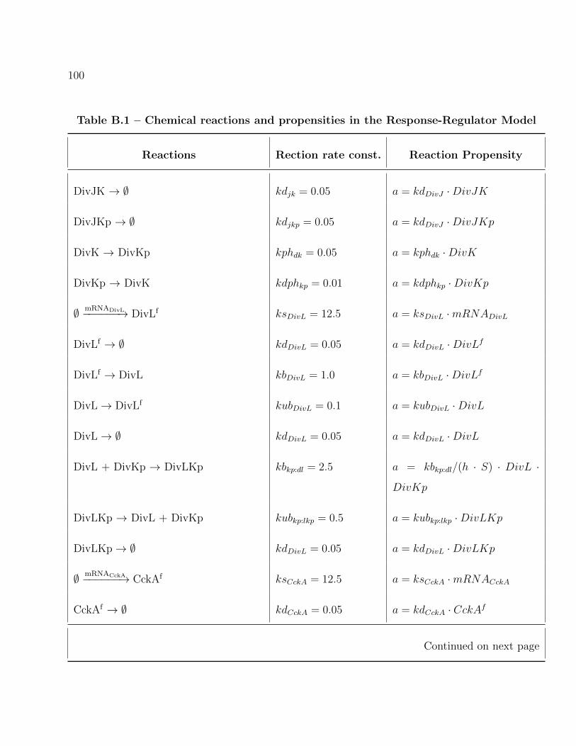
100
Table B.1 – Chemical reactions and propensities in the Response-Regulator Model
Reactions Rection rate const. Reaction Propensity
DivJK → ∅ kdjk = 0.05 a = kdDivJ ·DivJK
DivJKp → ∅ kdjkp = 0.05 a = kdDivJ ·DivJKp
DivK → DivKp kphdk = 0.05 a = kphdk ·DivK
DivKp → DivK kdphkp = 0.01 a = kdphkp ·DivKp
∅ mRNADivL−−−−−−→ DivLf ksDivL = 12.5 a = ksDivL ·mRNADivL
DivLf → ∅ kdDivL = 0.05 a = kdDivL ·DivLf
DivLf → DivL kbDivL = 1.0 a = kbDivL ·DivLf
DivL→ DivLf kubDivL = 0.1 a = kubDivL ·DivL
DivL→ ∅ kdDivL = 0.05 a = kdDivL ·DivL
DivL + DivKp → DivLKp kbkp:dl = 2.5 a = kbkp:dl/(h · S) · DivL ·
DivKp
DivLKp → DivL + DivKp kubkp:lkp = 0.5 a = kubkp:lkp ·DivLKp
DivLKp→ ∅ kdDivL = 0.05 a = kdDivL ·DivLKp
∅ mRNACckA−−−−−−→ CckAf ksCckA = 12.5 a = ksCckA ·mRNACckA
CckAf → ∅ kdCckA = 0.05 a = kdCckA · CckAf
Continued on next page

101
Table B.1 – Chemical reactions and propensities in the Response-Regulator Model
Reactions Rection rate const. Reaction Propensity
CckAf → CckAphos kbCckA = 1.0 a = kbCckA · CckAf
CckAphos→ CckAf kubCckA = 0.1 a = kubCckA · CckAphos
CckAphosDivL−−→ CckAkin kck = 10.0, Km = 0.5 a = kck
DivL4
DivL4+(Km·h·S)4
CckAkin → CckAphos kph:ck = 1.0 a = kph:ck · CckAkin
CckAkin → ∅ kdCckA = 0.05 a = kdCckA · CckAkin
CckAphos → ∅ kdCckA = 0.05 a = kdCckA · CckAphos
∅ mRNACtrA−−−−−−→ CtrA ksCtrA = 25.0 a = ksCtrA ·mRNACtrA
CtrA → ∅ kdCtrA = 0.05 a = kphCtrA · CtrA
CtrAp → ∅ kdCtrA = 0.05 a = kdphCtrAp · CtrAp
CtrACckAkin−−−−−→ CtrAp kphCtrA = 600.0 a = kdCtrA/(h · S) · CtrA ·
CckAkin
CtrApCckAphos−−−−−→ CtrA kdphCtrAp = 600.0 a = kdCtrA/(h · S) · CtrAp ·
CckAphos

102
Table B.2: Diffusive reactions and propensities in the Response-Regulator Model
Diffusive Jump Rate Const. Propensity
DivJfi → DivJf
i+1 Ddj = 10.0 a = Ddj/h2 ·DivJfi
DivJfi → DivJf
i−1 Ddj = 10.0 a = Ddj/h2 ·DivJfi
PleCfi → PleCf
i+1 Dpc = 10.0 a = Dpc/h2 · PleCf
i
PleCfi → PleCf
i−1 Dpc = 10.0 a = Dpc/h2 · PleCf
i
DivKi → DivKi+1 Ddk = 10.0 a = Ddk/h2 ·DivKi
DivKi → DivKi−1 Ddk = 10.0 a = Ddk/h2 ·DivKi
DivKpi → DivKpi+1 Ddk = 10.0 a = Ddk/h2 ·DivKpi
DivKpi → DivKpi−1 Ddk = 10.0 a = Ddk/h2 ·DivKpi
DivLfi → DivLf
i+1 Ddl = 10.0 a = Ddl/h2 ·DivLfi
DivLfi → DivLf
i−1 Ddl = 10.0 a = Ddl/h2 ·DivLfi
CckAfi → CckAf
i+1 Dck = 10.0 a = Dck/h2 · CckAfi
CckAfi → CckAf
i−1 Dck = 10.0 a = Dck/h2 · CckAfi
CtrAi → CtrAi+1 Dca = 10.0 a = Dca/h2 · CtrAi
CtrAi → CtrAi−1 Dca = 10.0 a = Dca/h2 · CtrAi
CtrApi → CtrApi+1 Dca = 10.0 a = Dca/h2 · CtrApi
Continued on next page

103
Table B.2 – Diffusive reactions and propensities in the Response-Regulator Model
Diffusive Jump Rection rate const. Reaction Propensity
CtrApi → CtrApi−1 Dca = 10.0 a = Dca/h2 · CtrApi
B.3 Result Figures

104
Figure B.1: The transformations of PleC kinase and phosphatase when interacting with
DivK and DivKp.
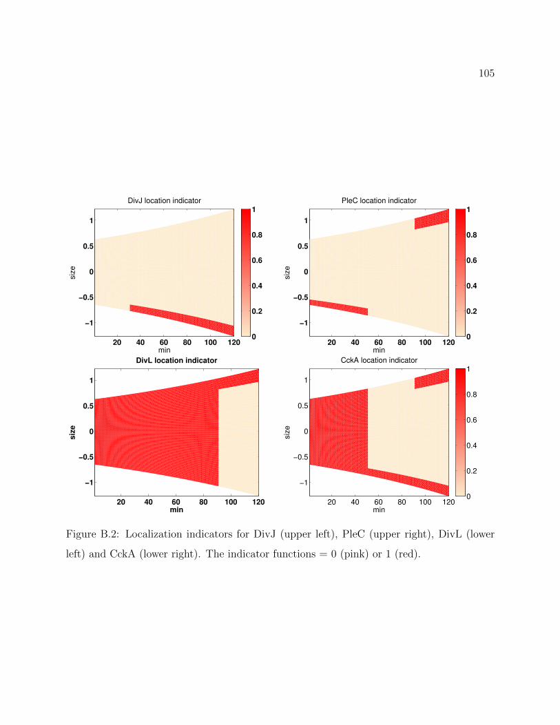
105
20 40 60 80 100 120
−1
−0.5
0
0.5
1
min
siz
e
DivJ location indicator
0
0.2
0.4
0.6
0.8
1
20 40 60 80 100 120
−1
−0.5
0
0.5
1
min
siz
e
PleC location indicator
0
0.2
0.4
0.6
0.8
1
20 40 60 80 100 120
−1
−0.5
0
0.5
1
min
siz
e
DivL location indicator
20 40 60 80 100 120
−1
−0.5
0
0.5
1
min
siz
e
CckA location indicator
0
0.2
0.4
0.6
0.8
1
Figure B.2: Localization indicators for DivJ (upper left), PleC (upper right), DivL (lower
left) and CckA (lower right). The indicator functions = 0 (pink) or 1 (red).

106
0 500 1000 1500 2000 2500 3000 3500 40000
0.1
0.2
0.3
0.4
0.5
0.6
population
pro
babili
ty
PleC:DivKp
DivLKp
free DivKp
0 100 200 300 400 5000
0.02
0.04
0.06
0.08
0.1
0.12
0.14
0.16
0.18
0.2
population
pro
babili
ty
free DivL
Figure B.3: Histograms of DivKp and free DivL in the early predivisional stage of the
Caulobacter cell cycle. Up: most DivKp molecules are complexed with PleC histidine kinase.
Bottom: Most DivL molecules are free to activate CckA kinase.

107
20 40 60 80 100 120
−1
−0.5
0
0.5
1
min
µm
total_DivJ
0
50
100
150
20 40 60 80 100 120
−1
−0.5
0
0.5
1
minµ
m
total_PleCkin
0
50
100
150
200
250
20 40 60 80 100 120
−1
−0.5
0
0.5
1
min
µm
total_PleCphos
0
50
100
150
200
250
20 40 60 80 100 120
−1
−0.5
0
0.5
1
min
µm
total_DivKp
0
50
100
150
200
250
300
350
400
450
500
20 40 60 80 100 120
−1
−0.5
0
0.5
1
min
µm
CckAkin
0
10
20
30
40
50
60
70
80
20 40 60 80 100 120
−1
−0.5
0
0.5
1
min
µm
CckAphos
0
10
20
30
40
50
60
70
80
20 40 60 80 100 120
−1
−0.5
0
0.5
1
min
µm
free_DivL
0
5
10
15
20
25
30
35
40
20 40 60 80 100 120
−1
−0.5
0
0.5
1
min
µm
CtrAp
0
5
10
15
20
25
30
35
40
Figure B.4: A typical stochastic simulation of regulatory proteins during the Caulobacter cell
cycle prior to cytokinesis. Colors indicate the numbers of protein molecules in each bin. DivJ
is synthesized throughout the cell cycle and becomes localized at the old pole after t = 30 min.
Transient co-localization of DivJ and PleC (t = 30 − 50 min) turns PleC into kinase form, before
PleC is cleared from the old pole (t = 50−90 min) and relocates (t = 90−120 min) to the new pole
(the nascent flagellated pole). Upon phosphorylation, DivK localizes to the poles of the cell, where
it binds with PleC histidine kinase. Despite the presence of phosphorylated DivK at the new pole
of the predivisional cell, DivL stays active (free DivL, unbound to DivKp) because PleC kinase
sequesters DivKp and prevents it from binding to DivL. In the swarmer stage, CckA is uniformly
distributed and stays as the kinase form. In the predivisional stage, CckA localizes to both poles.
Reactivation of DivL turns CckA into the kinase form at the swarmer pole, while CckA remains as
a phosphatase at the stalk pole. Consequently, the late predivisional cell establishes a gradient of
phosphorylated CtrA along its length with a high level of CtrAp at the new pole and a low level
at the old pole. Stochastic simulations generate temporally varying protein distributions similar to
the results of the deterministic model [106] with realistic fluctuations superimposed.

108
125 130 135 140 145 150−1.5
−1
−0.5
0
0.5
1
min
µm
total_DivJ
0
50
100
150
125 130 135 140 145 150−1.5
−1
−0.5
0
0.5
1
min
µm
total_PleCkin
0
50
100
150
200
250
125 130 135 140 145 150−1.5
−1
−0.5
0
0.5
1
min
µm
free_DivL
0
10
20
30
40
50
60
70
80
125 130 135 140 145 150−1.5
−1
−0.5
0
0.5
1
min
µm
CckAphos
0
10
20
30
40
50
60
70
80
125 130 135 140 145 150−1.5
−1
−0.5
0
0.5
1
min
µm
CckAkin
0
10
20
30
40
50
60
70
80
125 130 135 140 145 150−1.5
−1
−0.5
0
0.5
1
min
µm
CtrAp
0
10
20
30
40
50
60
Figure B.5: A typical stochastic simulation of regulatory proteins in the late predivisional
stage of the Caulobacter cell cycle. Colors indicate the numbers of protein molecules in
each bin. The bold black line marks the division plane, which separates the cell into two
compartments. In the lower half (the stalked cell) DivJ is actively phosphorylating DivK,
which inhibits CtrA phosphorylation. In the upper half (the nascent swarmer cell), there
is insufficient DivKp to keep PleC in the kinase form. As PleC transforms to phosphatase,
it dephosphorylates DivKp. Consequently, DivL is activated and CtrAp accumulates in the
swarmer cell.
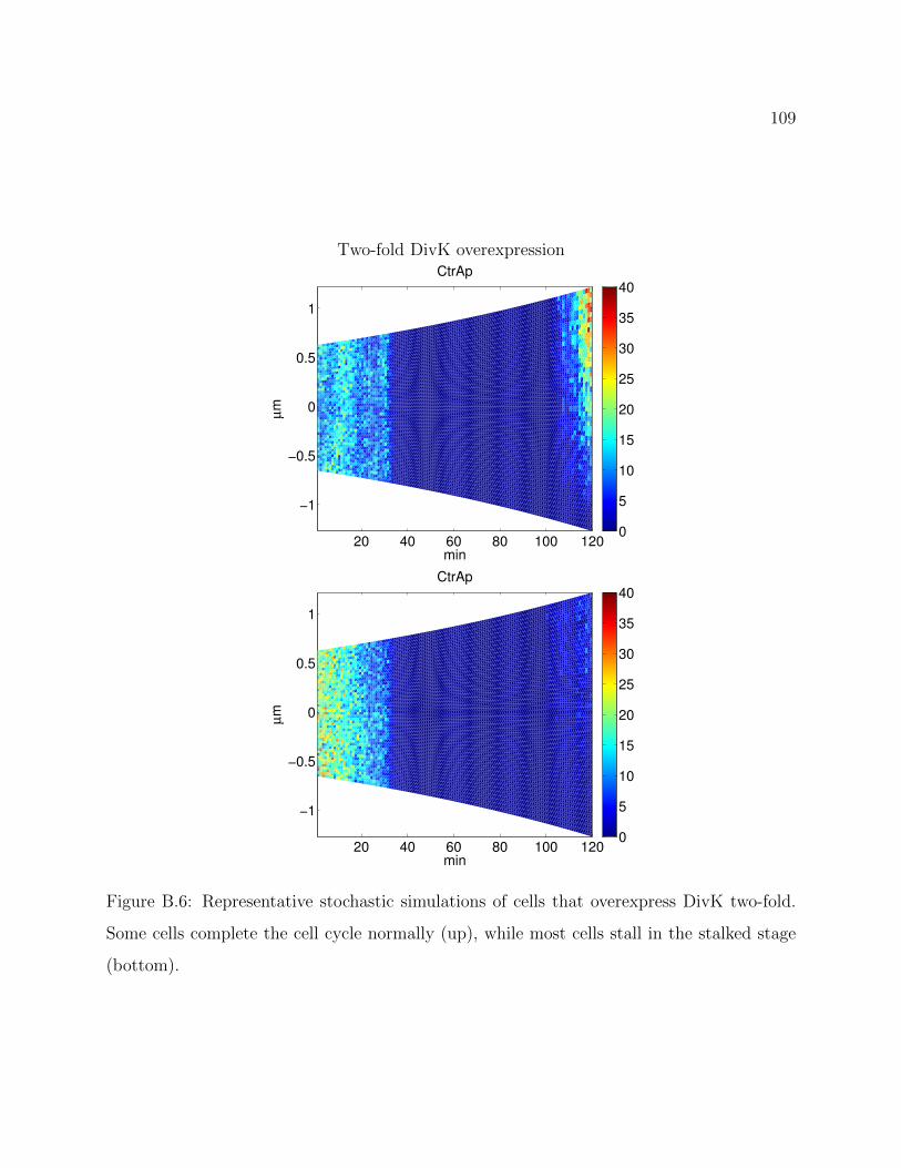
109
Two-fold DivK overexpression
20 40 60 80 100 120
−1
−0.5
0
0.5
1
min
µm
CtrAp
0
5
10
15
20
25
30
35
40
20 40 60 80 100 120
−1
−0.5
0
0.5
1
min
µm
CtrAp
0
5
10
15
20
25
30
35
40
Figure B.6: Representative stochastic simulations of cells that overexpress DivK two-fold.
Some cells complete the cell cycle normally (up), while most cells stall in the stalked stage
(bottom).

110
0 500 1000 1500 20000
0.1
0.2
0.3
0.4
0.5
CtrAp population
pro
ba
bil
ity
wild type2x DivK overexpression
Figure B.7: Histogram of total phosphorylated CtrA in the early predivisional stage.
Stochastic simulations show that some cells have a high population of CtrAp, which en-
ables them to complete the cell cycle as a wild-type cell would, while others stay in the stalk
stage and fail to divide.
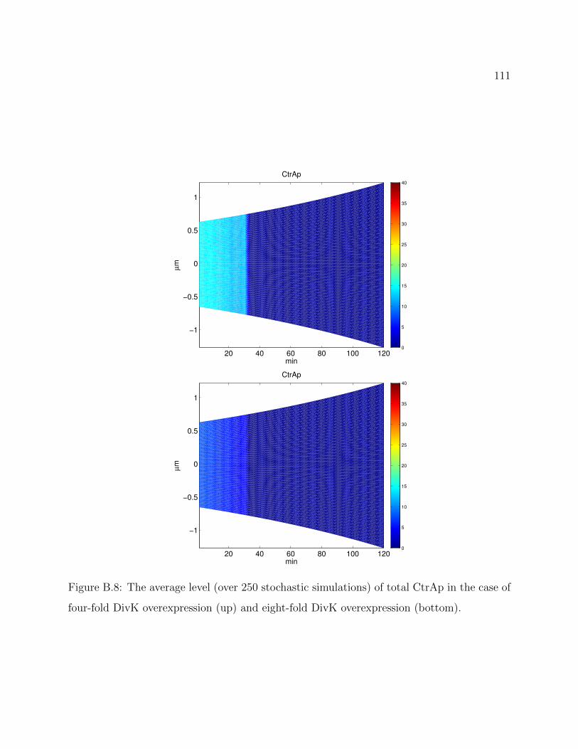
111
20 40 60 80 100 120
−1
−0.5
0
0.5
1
min
µm
CtrAp
0
5
10
15
20
25
30
35
40
20 40 60 80 100 120
−1
−0.5
0
0.5
1
min
µm
CtrAp
0
5
10
15
20
25
30
35
40
Figure B.8: The average level (over 250 stochastic simulations) of total CtrAp in the case of
four-fold DivK overexpression (up) and eight-fold DivK overexpression (bottom).

112
0 500 1000 1500 20000
0.05
0.1
0.15
0.2
0.25
0.3
0.35
0.4
CtrAp population
pro
babili
ty
wild type4x Overexpression8x Overexpression
Figure B.9: Histograms of CtrAp populations at t = 30 min. With eight-fold DivK overex-
pression, CtrA phosphorylation is greatly reduced in what should be the swarmer stage of
the cell cycle.
0 50 100 1500
200
400
600
800
1000
1200
1400
1600
1800
2000
time min
tota
l C
trA
p p
op
ula
tion
Figure B.10: Typical trajectories of the total numbers of CtrAp molecules during a wild-type
cell cycle. CtrAp populations are high in the swarmer stage and drop dramatically at the
swarmer-to-stalked transition, to allow the initiation of chromosome replication.

113
0 20 40 60 80 100 1200
0.05
0.1
0.15
0.2
0.25
0.3
0.35
0.4
0.45
0.5
time min
pro
babili
ty
∆divJ
wild type
Figure B.11: Histograms of swarmer-to-stalked transition times in wild-type cells and ∆divJ
mutant cells. The mean transition time is ∼ 42 min for wild-type cells and ∼ 49 min for
∆divJ mutant cells. ∆divJ mutant cells show a much larger variance of transition times.
The coefficient of variation of swarmer-to-stalked transition times is 14% for wild-type cells
and 29% for ∆divJ cells, in very good agreement with the COVs observed by Lin et al. [68]
for total cell cycle times. We conclude that depletion of divJ doesn’t stall the swarmer-to-
stalked transition for long, but it causes large fluctuations in the transition time.
0 500 1000 1500 2000 25000
0.05
0.1
0.15
0.2
0.25
DivKp population
pro
babili
ty
wild type
∆divJ
Figure B.12: Histograms of DivKp at t = 50 min in wild-type and ∆divJ cells.
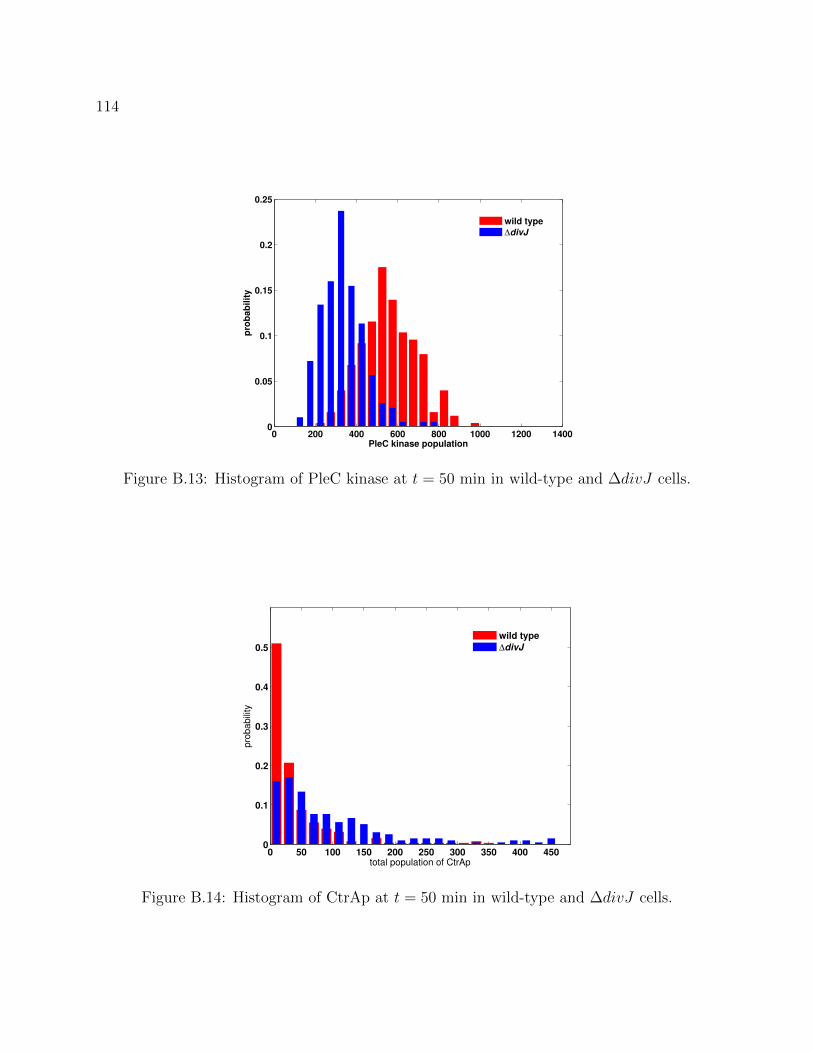
114
0 200 400 600 800 1000 1200 14000
0.05
0.1
0.15
0.2
0.25
PleC kinase population
pro
bab
ilit
y
wild type
∆divJ
Figure B.13: Histogram of PleC kinase at t = 50 min in wild-type and ∆divJ cells.
0 50 100 150 200 250 300 350 400 4500
0.1
0.2
0.3
0.4
0.5
total population of CtrAp
pro
ba
bili
ty
wild type
∆divJ
Figure B.14: Histogram of CtrAp at t = 50 min in wild-type and ∆divJ cells.

Appendix C
Supplement Materials
C.1 Model Details
Subramanian proposed an Activator Substrate-Depletion (A-SD) type Turing mechanism [105]
to explain the mechanisms behind PopZ bipolarization (Equation (C.1)).
∂[popZmRNA]
∂t= ksyn rna[popZgene]− kdeg mRNA[popZmRNA]− µ[popZmRNA]
+DmRNA∂2[popZmRNA]
∂x2,
∂[PopZm]
∂t= ksyn PopZ [popZmRNA]− kdeg PopZ [PopZm]
−kdnv[PopZm]− kaut[PopZm][PopZp]2 + kdepol[PopZp]
−µ[PopZm] +DPopZm∂2[PopZm]
∂x2,
∂[PopZp]
∂t= kdnv[PopZm] + kaut[PopZm][PopZp]2 − kdepol[PopZp]
−kdeg PopZ [PopZp]− µ[PopZp] +DPopZp∂2[PopZp]
∂x2,
(C.1)
115

116
where [PopZm] denotes the concentration level of PopZ monomers and [PopZp] for PopZ
polymers. Cell growth leads to dilute effect and µ is the growth rate along the cell axis.
In the stochastic model of PopZ bipolarization, the banana shaped Caulobacter cell is simpli-
fied and modeled as a one dimensional domain along its long axis. According to the multiple
grid discretization method, the corresponding one dimensional reaction-diffusion system is
discretized into 100 compartments (“bins”) for popZ mRNAs and PopZ polymers. Due to the
high diffusion rate constant, the one dimensional domain is discretized into 25 compartments
for PopZ monomers. In each compartment, all chemical reactions (listed in table C.1), as
well as all diffusive jumps, are simulated by “direct method” of SSA.
When a Caulobacter cell grows, new cell wall material is synthesized uniformly along the
long axis. Thus, during Caulobacter cell cycle, the length of each compartment grows expo-
nentially in time asdh
dt= µ · h. (C.2)
The new born swarmer cell of Caulobacter has the length of 1.3 µm. After 150 min cell
growth, it grows to 3.0 µm before cell division, with the growth rate µ = 0.0055 min−1.
Before DNA replication starts, there is only one copy of the bacterial chromosome, with its
origin of replication near the old pole. In the stochastic model, this gene is located at 20% of
the length from the end of old pole. At t = 50 min, chromosome replication and segregation
starts. A second copy of the chromosome translocates from the old pole to the new pole
(20% of the length from the new pole). The replicated gene takes a biased random walk
towards the new pole, with the drift rate vpopZ = 0.08 µm/min.
The stochastic simulation of the PopZ polarization model consists of two stages. A fixed cell
length stage is used to get the initial condition for the cell growth stage. Before the cell growth
starts, PopZ forms a focus in the old pole. Then the cell begins to grow exponentially, with
the rate constant µ = 0.005577 min−1. In the stochastic simulation, the cell size is updated
when one reaction or diffusion event happens. Between two reaction/diffusion events, the
cell size keeps constant, and so do the cell size related reaction propensities. In this model,

117
each time step is so small, hence this assumption and approximation are valid.
C.2 Rule Based Modeling in Reaction Diffusion Sys-
tem
With the spatial domain partition, the stochastic model consists of thousands of reaction
channels. It is not only inefficient to perform stochastic simulation on such a huge system,
but also difficult to analyze such a system. As reactions in all compartments are basically the
same, the idea of rule-based modeling technique [47] is applied to the stochastic simulation
of PopZ polarization model.
The rule based modeling was originally developed for the stochastic simulation on interaction
networks of multistate species. Multistate species exist naturally in biological systems, such
as proteins with multiple levels of phosphorylation or with various ligand binding sites [47].
The different binding configurations yield different biochemical species. In the conventional
modeling method, it requires one state variable for each different species, which results
in a large system that is inefficient to perform the stochastic simulation. The rule-based
modeling [47] was thus proposed for these complex multistate protein-ligand interaction
systems. In Hlavacek’s definition, a rule can be an individual reaction or an entire reaction
family [47]. For example, suppose protein R has three binding sites, and a ligand L binds to
the first binding site. A rule might include all reactions that bind a ligand L onto the first
binding site, regardless of the other two site:
Ropen,∗,∗ + Lkb−→ RL,∗,∗ (C.3)
where the subscripts of a species describe the configuration of all its binding site. An asterisk
mark indicates any possible states for a certain site. In the rule-based modeling, one rule is
sufficient to represent a family of reactions, which yields a much smaller system.
In reaction-diffusion systems, reactions in all compartments are fundamentally the same.
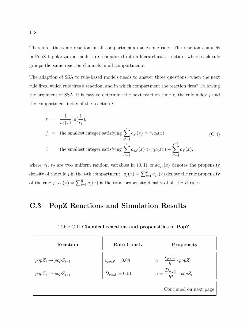
118
Therefore, the same reaction in all compartments makes one rule. The reaction channels
in PopZ bipolarization model are reorganized into a hierarchical structure, where each rule
groups the same reaction channels in all compartments.
The adaption of SSA to rule-based models needs to answer three questions: when the next
rule fires, which rule fires a reaction, and in which compartment the reaction fires? Following
the argument of SSA, it is easy to determine the next reaction time τ , the rule index j and
the compartment index of the reaction i.
τ =1
a0(x)ln(
1
r1
),
j = the smallest integer satisfying
j∑j′=1
aj′(x) > r2a0(x),
i = the smallest integer satisfyingi∑
i′=1
aj,i′(x) > r2a0(x)−j−1∑j′=1
aj′(x).
(C.4)
where r1, r2 are two uniform random variables in (0, 1), andaj,i(x) denotes the propensity
density of the rule j in the i-th compartment. aj(x) =∑K
i=1 aj,i(x) denote the rule propensity
of the rule j. a0(x) =∑R
j=1 aj(x) is the total propensity density of all the R rules.
C.3 PopZ Reactions and Simulation Results
Table C.1: Chemical reactions and propensities of PopZ
Reaction Rate Const. Propensity
popZi → popZi−1 vpopZ = 0.08 a =vpopZh· popZi
popZi → popZi+1 DpopZ = 0.01 a =DpopZ
h2· popZi
Continued on next page

119
Table C.1 – Chemical reactions and propensities of PopZ (Continued)
Reactions Rection rate const. Reaction Propensity
popZi → popZi−1 DpopZ = 0.01 a =DpopZ
h2· genei
∅ popZi−−−→ mRNAi ksyn rna = 0.625 a = ksyn rna · popZi
mRNAi → ∅ kdeg mRNA = 0.25 a = kdeg rna ·mRNAi
mRNAi → mRNAi+1 DmRNA = 0.05 a =DmRNA
h2·mRNAi
mRNAi → mRNAi−1 DmRNA = 0.05 a =DmRNA
h2·mRNAi
∅ mRNAi−−−−→ PopZmi ksyn PopZ = 40.0 a = ksyn PopZ ·mRNAi
PopZmi → ∅ kdeg popZ = 0.05 a = kdeg PopZ · PopZmi
PopZmi → PopZmi+1 DPopZm = 10.0 a =Dm
h2· PopZmi
PopZmi → PopZmi−1 DPopZm = 10.0 a =Dm
h2· PopZmi
PopZmi → PopZpi kdnv = 12.0 a = kdnv · PopZmi
PopZmi + 2PopZpi → 3PopZpi kaut = 1.8e− 5 a =kauth2· PopZmi · PopZp2
i
PopZpi → PopZmi kdepol = 0.1 a = kdepol · PopZpi
PopZpi → ∅ kdeg PopZp = 0.05 a = kdeg PopZp · PopZpi
PopZpi → PopZpi+1 DPopZp = 0.001 a =DPopZp
h2· PopZpi
PopZpi → PopZpi−1 DPopZp = 0.001 a =DPopZp
h2· PopZpi

120
C.4 FtsZ Reactions and Simulation Results
Table C.2: Chemical reactions and propensities of FtsZ
Reaction Rate Const. Propensity
∅ → MipZi ksyn MipZ = 80 a = ksyn MipZ · h
MipZi → ∅ kdeg MipZ = 0.25 a = kdeg MipZ ·MipZi
MipZi → MipZi+1 DMipZ = 10.0 a =DMipZ
h2·MipZi
MipZi → mRNAi−1 DMipZ = 10.0 a =DMipZ
h2·MipZi
MipZiPopZi−−−→ MipZbi kbnd MipZ = 0.0125 a = kbnd MipZ/h · PopZi ·MipZi
MipZbi → MipZ kubd MipZ = 0.1 a = kubd MipZ ·MipZi
∅ → FtsZmi ksyn FtsZ = 160.0 a = ksyn FtsZ · h
FtsZmi → ∅ kdeg F tsZm = 0.25 a = kdeg F tsZm · FtsZmi
FtsZmi → FtsZmi+1 DFtsZm = 10.0 a =DFtsZm
h2· FtsZmi
FtsZmi → FtsZmi−1 DFtsZm = 10.0 a =DFtsZm
h2· FtsZmi
FtsZmi → FtsZpi kdnv FtsZ = 300.0 a = kdnv FtsZ · FtsZmi
FtsZmiFtsZpi−−−→ FtsZpi kaut F tsZ = 2.5e− 4 a =
kaut F tsZh2
· FtsZmi · FtsZp2i
FtsZpi → FtsZmi kdepol F tsZ = 0.0125 a = kdepol F tsZ/h ·MipZbi · FtsZpi
FtsZpi → ∅ kdeg F tsZp = 0.075 a = kdeg F tsZp · FtsZpi
Continued on next page

121
Table C.2 – Chemical reactions and propensities of FtsZ (Continued)
Reactions Rection rate const. Reaction Propensity
FtsZpi → FtsZpi+1 DFtsZp = 0.01 a =DFtsZp
h2· FtsZpi
FtsZpi → FtsZpi−1 DFtsZp = 0.01 a =DFtsZp
h2· FtsZpi

122
0 50 100 150−1.5
−1
−0.5
0
0.5
1
1.5
po
sit
ion
x
time t
popZ gene
Figure C.1: Stochastic simulation result of PopZ polarization model. Up left: One popZ
gene is constantly present at 20% of cell length from the old pole end. The chromosome
replication starts at t = 50 min and the replicated chromosome translocates across the cell
until it reaches the position of 20% cell length from the new pole end. Up right: popZ mNRA
is synthesized from the two genes. Due to the short life time (half life time of 2 ∼ 3 min)
and slow diffusion (0.05µm2/min), mNRA can not move far from popZ gene site. Bottom:
PopZ shows a unipolar-to-bipolar transition at around t = 75 min.

123
50 100 1500
0.05
0.1
0.15
0.2
time (min)
fra
cti
on
of
ce
lls
gene segregation ends
PopZ becomes bipolar
1.5 2 2.5 30
0.05
0.1
0.15
0.2
0.25
cell size (µm)
fra
cti
on
of
ce
lls
gene segregation ends
PopZ becomes bipolar
Figure C.2: Histogram of time (top) and cell length (bottom) when popZ gene segregation
is complete (green) and PopZ becomes bipolar (red).

124
20 40 60 80 100 120 140−1.5
−1
−0.5
0
0.5
1
time t
cell len
gth
µm
MipZ
0
5
10
15
20
25
30
35
40
20 40 60 80 100 120 140−1.5
−1
−0.5
0
0.5
1
time t
cell len
gth
µm
FtsZ
0
20
40
60
80
100
120
140
160
180
200
Figure C.3: The spatiotemporal pattern of stochastic simulation on FtZ polarization model.
Up: MipZ assembles the distribution of PopZ. MipZ binds to the chromosome front in
swarmer cells. After the chromosome segregation stars, MipZ translocates to the new pole
together with the replicated chromosome. Bottom: In the swarmer cell, MipZ stays in the old
pole and repels FtsZ polymers to the new pole. After the chromosome segregation completes,
FtsZ shifts towards the middle of the cell, where MipZ level is lowest.

Bibliography
[1] P. Aldridge, R. Paul, P. Goymer, P. Rainey, and U. Jenal. Role of the GGDEF
regulator PleD in polar development of Caulobacter crescentus. Molecular Microbiology,
47(6):1695–1708, 2003.
[2] S. S. Andrews and D. Bray. Stochastic simulation of chemical reactions with spatial
resolution and single molecule detail. Physical Biology, 1:137–151, 2004.
[3] P. S. Angelastro, O. Sliusarenko, and C. Jacobs-Wagner. Polar localization of the
CckA histidine kinase and cell cycle periodicity of the essential master regulator CtrA
in Caulobacter crescentus. Journal of Bacteriology, 192(2):539–552, 2010.
[4] F. Baras and M. M. Mansour. Reaction-diffusion master equation: A comparison with
microscopic simulations. Physical Review E, 54:6139–6148, Dec 1996.
[5] B. Bayati, P. Chatelain, and P. Koumoutsakos. Adaptive mesh refinement for stochas-
tic reaction-diffusion processes. Journal of Computational Physics, 230(1):13–26, 2011.
[6] J. A. Bernstein, A. B. Khodursky, P. H. Lin, S. Lin-Chao, and S. N. Cohen. Global
analysis of mRNA decay and abundance in Escherichia coli at single-gene resolution
using two-color fluorescent dna microarrays. Proceedings of the National Academy of
Sciences, 99(15):9697–9702, 2002.
[7] G. R. Bowman, L. R. Comolli, G. M. Gaietta, M. Fero, S.-H. Hong, Y. Jones, J. H.
Lee, K. H. Downing, M. H. Ellisman, H. H. McAdams, and L. Shapiro. Caulobacter
125

126
PopZ forms a polar subdomain dictating sequential changes in pole composition and
function. Molecular Microbiology, 76(1):173–189, 2010.
[8] G. R. Bowman, L. R. Comolli, J. Zhu, M. Eckart, M. Koenig, K. H. Downing, W. Mo-
erner, T. Earnest, and L. Shapiro. A polymeric protein anchors the chromosomal
origin/ParB complex at a bacterial cell pole. Cell, 134(6):945–955, 2008.
[9] G. R. Bowman, A. I. Lyuksyutova, and L. Shapiro. Bacterial polarity. Current Opinion
in Cell Biology, 23(1):71–77, 2011.
[10] C. V. D. Broeck, W. Horsthemke, and M. Malek-Mansour. On the diffusion oper-
ator of the multivariate master equation. Physica A: Statistical Mechanics and its
Applications, 89(2):339–352, 1977.
[11] Y. Cao and R. Erban. Stochastic Turing patterns: Analysis of compartment-based
approaches. Bulletin of Mathematical Biology, 76(12):3051–3069, 2014.
[12] Y. Cao, D. T. Gillespie, and L. R. Petzold. The slow-scale stochastic simulation
algorithm. The Journal of Chemical Physics, 122(1):014116, 2005.
[13] Y. Cao, D. T. Gillespie, and L. R. Petzold. Efficient step size selection for the tau-
leaping simulation method. The Journal of Chemical Physics, 124(4):044109, 2006.
[14] Y. Cao, H. Li, and L. Petzold. Efficient formulation of the stochastic simulation algo-
rithm for chemically reacting systems. The Journal of Chemical Physics, 121(9):4059–
4067, 2004.
[15] Y. Cao and D. C. Samuels. Discrete stochastic simulation methods for chemically
reacting systems. In Computer Methods, Part A, volume 454 of Methods in Enzymology,
pages 115–140. Academic Press, 2009.
[16] G. Charbon, M. T. Cabeen, and C. Jacobs-Wagner. Bacterial intermediate filaments:
in vivo assembly, organization, and dynamics of crescentin. Genes & Development,
23(9):1131–1144, 2009.

127
[17] J. Collier, S. R. Murray, and L. Shapiro. DnaA couples DNA replication and the
expression of two cell cycle master regulators. The EMBO Journal, 25(2):346–356,
2006.
[18] J. Collier and L. Shapiro. Spatial complexity and control of a bacterial cell cycle.
Current Opinion in Biotechnology, 18(4):333–340, 2007.
[19] P. D. Curtis and Y. V. Brun. Getting in the loop: Regulation of development in
Caulobacter crescentus. Microbiology and Molecular Biology Reviews, 74(1):13–41,
2010.
[20] M. Doi. Stochastic theory of diffusion-controlled reaction. Journal of Physics A:
Mathematical and General, 9(9):1479, 1976.
[21] V. T. dos Santos, A. W. Bisson-Filho, and F. J. Gueiros-Filho. DivIVA-mediated polar
localization of ComN, a posttranscriptional regulator of Bacillus subtilis. Journal of
Bacteriology, 194(14):3661–3669, 2012.
[22] B. Drawert, M. J. Lawson, L. Petzold, and M. Khammash. The diffusive finite state
projection algorithm for efficient simulation of the stochastic reaction-diffusion master
equation. The Journal of Chemical Physics, 132(7):074101, 2010.
[23] G. Ebersbach, A. Briegel, G. J. Jensen, and C. Jacobs-Wagner. A self-associating pro-
tein critical for chromosome attachment, division, and polar organization in Caulobac-
ter. Cell, 134(6):956–968, 2008.
[24] A. Einstein. Investigations on the theory of the brownian movement. Annalen der
Physik, page 4036262, 1905.
[25] J. Elf and M. Ehrenberg. Spontaneous separation of bi-stable biochemical systems into
spatial domains of opposite phases. Systems Biology, IEE Proceedings, 1(2):230–236,
2004.

128
[26] R. Erban and S. J. Chapman. Stochastic modelling of reaction-diffusion processes:
algorithms for bimolecular reactions. Physical Biology, 6(4):046001, 2009.
[27] D. Fange, O. G. Berg, P. Sjberg, and J. Elf. Stochastic reaction-diffusion kinetics in the
microscopic limit. Proceedings of the National Academy of Sciences, 107(46):19820–
19825, 2010.
[28] N. Fedoroff and W. Fontana. Small numbers of big molecules. Science, 297(5584):1129–
1131, 2002.
[29] A. Fick. Ueber diffusion. Annalen der Physik, 170(1):59–86, 1855.
[30] A. Fick. On liquid diffusion. Journal of Membrane Science, 100(1):33–38, 1995.
[31] M. B. Flegg, S. J. Chapman, and R. Erban. The two-regime method for optimiz-
ing stochastic reaction–diffusion simulations. Journal of The Royal Society Interface,
9(70):859–868, 2012.
[32] C. Gardiner, K. McNeil, D. Walls, and I. Matheson. Correlations in stochastic theories
of chemical reactions. Journal of Statistical Physics, 14:307–331, 1976.
[33] M. A. Gibson and J. Bruck. Efficient exact stochastic simulation of chemical sys-
tems with many species and many channels. The Journal of Physical Chemistry A,
104(9):1876–1889, 2000.
[34] A. Gierer and H. Meinhardt. A theory of biological pattern formation. Kybernetik,
12(1):30–39, 1972.
[35] D. T. Gillespie. A general method for numerically simulating the stochastic time
evolution of coupled chemical reactions. Journal of Computational Physics, 22(4):403–
434, 1976.
[36] D. T. Gillespie. Exact stochastic simulation of coupled chemical reactions. The Journal
of Physical Chemistry, 81(25):2340–2361, 1977.

129
[37] D. T. Gillespie. A rigorous derivation of the chemical master equation. Physica A:
Statistical Mechanics and its Applications, 188(1-3):404–425, 1992.
[38] D. T. Gillespie. The chemical Langevin equation. The Journal of Chemical Physics,
113(1):297–306, 2000.
[39] D. T. Gillespie. Approximate accelerated stochastic simulation of chemically reacting
systems. The Journal of Chemical Physics, 115(4):1716–1733, 2001.
[40] D. T. Gillespie. Stochastic simulation of chemical kinetics. Annual Review of Physical
Chemistry, 58(1):35–55, 2007.
[41] D. T. Gillespie and L. R. Petzold. Improved leap-size selection for accelerated stochastic
simulation. The Journal of Chemical Physics, 119(16):8229–8234, 2003.
[42] E. D. Goley, A. A. Iniesta, and L. Shapiro. Cell cycle regulation in Caulobacter :
location, location, location. Journal of Cell Science, 120(20):3501–3507, 2007.
[43] E. L. Haseltine and J. B. Rawlings. Approximate simulation of coupled fast and
slow reactions for stochastic chemical kinetics. The Journal of Chemical Physics,
117(15):6959–6969, 2002.
[44] J. Hattne, D. Fange, and J. Elf. Stochastic reaction-diffusion simulation with MesoRD.
Bioinformatics, 21(12):2923–2924, 2005.
[45] S. Hellander, A. Hellander, and L. Petzold. Reaction-diffusion master equation in the
microscopic limit. Physical Review E, 85:042901, Apr 2012.
[46] A. C. Hindmarsh. ODEPACK, a systematized collection of ODE solvers. In R. S.
Stepleman, editor, Scientific Computing, pages 55–64, Amsterdam, 1983. North-
Holland.
[47] W. S. Hlavacek, J. R. Faeder, M. L. Blinov, A. S. Perelson, and B. Goldstein. The
complexity of complexes in signal transduction. Biotechnology and Bioengineering,
84(7):783–794, 2003.
130
[48] J. Holtzendorff, D. Hung, P. Brende, A. Reisenauer, P. H. Viollier, H. H. McAdams,
and L. Shapiro. Oscillating global regulators control the genetic circuit driving a
bacterial cell cycle. Science, 304(5673):983–987, 2004.
[49] M. Howard. A mechanism for polar protein localization in bacteria. Journal of Molec-
ular Biology, 335(2):655–663, 2004.
[50] D. Y. Hung and L. Shapiro. A signal transduction protein cues proteolytic events
critical to Caulobacter cell cycle progression. Proceedings of the National Academy of
Sciences, 99(20):13160–13165, 2002.
[51] A. A. Iniesta, P. T. McGrath, A. Reisenauer, H. H. McAdams, and L. Shapiro. A
phospho-signaling pathway controls the localization and activity of a protease complex
critical for bacterial cell cycle progression. Proceedings of the National Academy of
Sciences, 103(29):10935–10940, 2006.
[52] S. A. Isaacson. The reaction-diffusion master equation as an asymptotic approximation
of diffusion to a small target. SIAM Journal on Applied Mathematics, 70(1):77–111,
2009.
[53] S. A. Isaacson. A convergent reaction-diffusion master equation. The Journal of
Chemical Physics, 139(5):054101, 2013.
[54] U. Jenal and T. Fuchs. An essential protease involved in bacterial cell-cycle control.
The EMBO Journal, 17(19):5658–5669, 1998.
[55] U. Jenal and M. Y. Galperin. Single domain response regulators: molecular switches
with emerging roles in cell organization and dynamics. Current Opinion in Microbiol-
ogy, 12(2):152–160, 2009.
[56] E. M. Judd, K. R. Ryan, W. E. Moerner, L. Shapiro, and H. H. McAdams. Fluo-
rescence bleaching reveals asymmetric compartment formation prior to cell division

131
in Caulobacter. Proceedings of the National Academy of Sciences, 100(14):8235–8240,
2003.
[57] J. Keizer. Nonequilibrium statistical thermodynamics and the effect of diffusion on
chemical reaction rates. The Journal of Physical Chemistry, 86(26):5052–5067, 1982.
[58] D. Kiekebusch, K. Michie, L.-O. Essen, J. Lwe, and M. Thanbichler. Localized dimer-
ization and nucleoid binding drive gradient formation by the bacterial cell division
inhibitor MipZ. Molecular Cell, 46(3):245–259, 2012.
[59] S. Kondo and T. Miura. Reaction-diffusion model as a framework for understanding
biological pattern formation. Science, 329(5999):1616–1620, 2010.
[60] Y. Kuramoto. Effects of diffusion on the fluctuations in open chemical systems.
Progress of Theoretical Physics, 52(2):711–713, 1974.
[61] G. Laloux and C. Jacobs-Wagner. Spatiotemporal control of PopZ localization through
cell cycle-coupled multimerization. The Journal of Cell Biology, 201(6):827–841, 2013.
[62] H. Lam, J.-Y. Matroule, and C. Jacobs-Wagner. The asymmetric spatial distribution
of bacterial signal transduction proteins coordinates cell cycle events. Developmental
Cell, 5(1):149–159, 2003.
[63] M. T. Laub, L. Shapiro, and H. H. McAdams. Systems biology of Caulobacter. Annual
Review of Genetics, 41(1):429–441, 2007.
[64] F. Li, M. Chen, Y. Cao, and R. Erban. Reaction time for trimolecular reactions in one-
dimensional compartment-based reaction-diffusion models. Physical Review E, 2016.
To be submitted.
[65] H. Li and L. Petzold. Logarithmic direct method for discrete stochastic simulation of
chemically reacting systems. Technical report, 2006.

132
[66] S. Li, P. Brazhnik, B. Sobral, and J. J. Tyson. A quantitative study of the division
cycle of Caulobacter crescentus stalked cells. PLoS Computational Biology, 4(1):e9, 01
2008.
[67] S. Li, P. Brazhnik, B. Sobral, and J. J. Tyson. Temporal controls of the asymmetric cell
division cycle in Caulobacter crescentus. PLoS Computational Biology, 5(8):e1000463,
08 2009.
[68] Y. Lin, S. Crosson, and N. F. Scherer. Single-gene tuning of Caulobacter cell cycle
period and noise, swarming motility, and surface adhesion. Molecular Systems Biology,
6(1), 2010.
[69] J. Lipkov, K. C. Zygalakis, S. J. Chapman, and R. Erban. Analysis of Brownian
dynamics simulations of reversible bimolecular reactions. SIAM Journal on Applied
Mathematics, 71(3):714–730, 2011.
[70] Z. Liu, Y. Pu, F. Li, C. A. Shaffer, S. Hoops, J. J. Tyson, and Y. Cao. Hybrid modeling
and simulation of stochastic effects on progression through the eukaryotic cell cycle.
The Journal of Chemical Physics, 136(3):034105, 2012.
[71] W. Margolin. FtsZ and the division of prokaryotic cells and organelles. Nature Reviews
Molecular Cell Biology, 6(11):862–871, Nov 2005.
[72] T. T. Marquez-Lago and K. Burrage. Binomial tau-leap spatial stochastic simulation
algorithm for applications in chemical kinetics. The Journal of Chemical Physics,
127(10):104101, 2007.
[73] J.-Y. Matroule, H. Lam, D. T. Burnette, and C. Jacobs-Wagner. Cytokinesis monitor-
ing during development: Rapid pole-to-pole shuttling of a signaling protein by localized
kinase and phosphatase in Caulobacter. Cell, 118(5):579–590, 2004.
[74] H. McAdams and A. Arkin. Stochastic mechanisms in geneexpression. Proceedings of
the National Academy of Sciences, 94(3):814–819, 1997.

133
[75] J. M. McCollum, G. D. Peterson, C. D. Cox, M. L. Simpson, and N. F. Samatova. The
sorting direct method for stochastic simulation of biochemical systems with varying
reaction execution behavior. Computational Biology and Chemistry, 30(1):39–49, 2006.
[76] P. T. McGrath, A. A. Iniesta, K. R. Ryan, L. Shapiro, and H. H. McAdams. A
dynamically localized protease complex and a polar specificity factor control a cell
cycle master regulator. Cell, 124(3):535–547, 2006.
[77] D. A. McQuarrie. Stochastic approach to chemical kinetics. Journal of Applied Prob-
ability, 4(3):413–478, 1967.
[78] R. Milo, P. Jorgensen, U. Moran, G. Weber, and M. Springer. Bionumbers—the
database of key numbers in molecular and cell biology. Nucleic Acids Research,
38(suppl 1):D750–D753, 2010.
[79] E. W. Montroll. Random walks on lattices. iii. calculation of firstpassage times with
application to exciton trapping on photosynthetic units. Journal of Mathematical
Physics, 10(4):753–765, 1969.
[80] E. W. Montroll and G. H. Weiss. Random walks on lattices. II. Journal of Mathematical
Physics, 6(2):167–181, 1965.
[81] E. Munro and B. Bowerman. Cellular symmetry breaking during Caenorhabditis ele-
gans development. Cold Spring Harbor Perspectives in Biology, 1(4), 2009.
[82] B. Munsky and M. Khammash. The finite state projection algorithm for the solution
of the chemical master equation. The Journal of Chemical Physics, 124(4):044104,
2006.
[83] G. Nicolis and I. Prigogine. Self-organization in nonequilibrium systems: from dissi-
pative structures to order through fluctuations. J. Wiley and sons, New York, London,
Sydney, 1977.

134
[84] N. L. Novere and T. S. Shimizu. StochSim: modelling of stochastic biomolecular
processes. Bioinformatics, 17:575–576, 2001.
[85] R. Paul, T. Jaeger, S. Abel, I. Wiederkehr, M. Folcher, E. G. Biondi, M. T. Laub, and
U. Jenal. Allosteric regulation of histidine kinases by their cognate response regulator
determines cell fate. Cell, 133(3):452–461, 2008.
[86] J. M. Pedraza and J. Paulsson. Effects of molecular memory and bursting on fluctua-
tions in gene expression. Science, 319(5861):339–343, 2008.
[87] J. J. Petricka, J. M. Van Norman, and P. N. Benfey. Symmetry breaking in plants:
Molecular mechanisms regulating asymmetric cell divisions in Arabidopsis. Cold Spring
Harbor Perspectives in Biology, 1(5), 2009.
[88] K. E. Prehoda. Polarization of Drosophila neuroblasts during asymmetric division.
Cold Spring Harbor Perspectives in Biology, 1(2), 2009.
[89] J. L. Ptacin, S. F. Lee, E. C. Garner, E. Toro, M. Eckart, L. R. Comolli, W. Moerner,
and L. Shapiro. A spindle-like apparatus guides bacterial chromosome segregation.
Nature Cell Biology, 12(8):791–798, 2010.
[90] E. M. Quardokus, N. Din, and Y. V. Brun. Cell cycle and positional constraints on
FtsZ localization and the initiation of cell division in Caulobacter crescentus. Molecular
Microbiology, 39(4):949–959, 2001.
[91] K. C. Quon, B. Yang, I. J. Domian, L. Shapiro, and G. T. Marczynski. Negative
control of bacterial DNA replication by a cell cycle regulatory protein that binds at
the chromosomeorigin. Proceedings of the National Academy of Sciences, 95(1):120–
125, 1998.
[92] K. Radhakrishnan and A. C. Hindmarsh. Description and use of LSODE, the Livermore
Solver for Ordinary Differential Equations. Technical report, Lawrence Livermore
National Laboratory, 1993.

135
[93] C. V. Rao and A. P. Arkin. Stochastic chemical kinetics and the quasi-steady-state
assumption: Application to the gillespie algorithm. The Journal of Chemical Physics,
118(11):4999–5010, 2003.
[94] D. Z. Rudner and R. Losick. Protein subcellular localization in bacteria. Cold Spring
Harbor Perspectives in Biology, 2(4), 2010.
[95] H. Salis and Y. Kaznessis. Accurate hybrid stochastic simulation of a system of coupled
chemical or biochemical reactions. The Journal of Chemical Physics, 122(5):54103,
2005.
[96] H. Salis, V. Sotiropoulos, and Y. Kaznessis. Multiscale Hy3S: Hybrid stochastic sim-
ulation for supercomputers. BMC Bioinformatics, 7(1):93, 2006.
[97] M. Samoilov, S. Plyasunov, and A. P. Arkin. Stochastic amplification and signaling in
enzymatic futile cycles through noise-induced bistability with oscillations. Proceedings
of the National Academy of Sciences of the United States of America, 102(7):2310–
2315, 2005.
[98] W. B. Schofield, H. C. Lim, and C. Jacobs-Wagner. Cell cycle coordination and reg-
ulation of bacterial chromosome segregation dynamics by polarly localized proteins.
The EMBO Journal, 29(18):3068–3081, 2010.
[99] L. Shapiro, H. H. McAdams, and R. Losick. Generating and exploiting polarity in
bacteria. Science, 298(5600):1942–1946, 2002.
[100] D. Siegal-Gaskins and S. Crosson. Tightly regulated and heritable division control in
single bacterial cells. Biophysical Journal, 95(4):2063–2072, 2008.
[101] A. Slepoy, A. P. Thompson, and S. J. Plimpton. A constant-time kinetic monte carlo
algorithm for simulation of large biochemical reaction networks. The Journal of Chem-
ical Physics, 128(20):205101, 2008.

136
[102] O. Sliusarenko, J. Heinritz, T. Emonet, and C. Jacobs-Wagner. High-throughput,
subpixel precision analysis of bacterial morphogenesis and intracellular spatio-temporal
dynamics. Molecular Microbiology, 80(3):612–627, 2011.
[103] G. Stein, A. van Wijnen, J. Stein, J. Lian, M. Montecino, J. Choi, K. Zaidi, and
A. Javed. Intranuclear trafficking of transcription factors: implications for biological
control. Journal of Cell Science, 113(14):2527–2533, 2000.
[104] K. Subramanian, M. R. Paul, and J. J. Tyson. Potential role of a bistable histidine
kinase switch in the asymmetric division cycle of Caulobacter crescentus. PLoS Com-
putational Biology, 9(9):e1003221, 09 2013.
[105] K. Subramanian, M. R. Paul, and J. J. Tyson. De novo production of Turing activator
generates polarity in pattern formation. In Advances In Systems AND Synnthetic
Biology, pages 131–142, 3 2014.
[106] K. Subramanian, M. R. Paul, and J. J. Tyson. Dynamical localization of DivL and PleC
in the asymmetric division cycle of Caulobacter crescentus : A theoretical investigation
of alternative models. PLoS Computational Biology, 11(7):e1004348, 07 2015.
[107] Y. Taniguchi, P. J. Choi, G.-W. Li, H. Chen, M. Babu, J. Hearn, A. Emili, and X. S.
Xie. Quantifying E. coli proteome and transcriptome with single-molecule sensitivity
in single cells. Science, 329(5991):533–538, 2010.
[108] M. Thanbichler. Spatial regulation in Caulobacter crescentus. Current Opinion in
Microbiology, 12(6):715–721, 2009.
[109] M. Thanbichler and L. Shapiro. MipZ, a spatial regulator coordinating chromosome
segregation with cell division in Caulobacter. Cell, 126(1):147–162, 2006.
[110] C. Tsokos, B. Perchuk, and M. Laub. A dynamic complex of signaling proteins uses
polar localization to regulate cell-fate asymmetry in Caulobacter crescentus. Develop-
mental Cell, 20(3):329–341, 2011.

137
[111] A. Turing. The chemical basis of morphogenesis. Philosophical Transactions of the
Royal Society B, 237:37–72, 1952.
[112] J. S. van Zon and P. R. ten Wolde. Greens-function reaction dynamics: A particle-
based approach for simulating biochemical networks in time and space. The Journal
of Chemical Physics, 123(23):234910, 2005.
[113] J. S. van Zon and P. R. ten Wolde. Simulating biochemical networks at the particle
level and in time and space: Green’s function reaction dynamics. Physical Review
Letters, 94:128103, Apr 2005.
[114] M. von Smoluchowski. Zur kinetischen theorie der Brownschen molekularbewegung
und der suspensionen. Annalen der Physik, 326(14):756–780, 1906.
[115] L. J. Wu and J. Errington. RacA and the Soj-Spo0J system combine to effect po-
lar chromosome segregation in sporulating Bacillus subtilis. Molecular Microbiology,
49(6):1463–1475, 2003.
[116] D. Zenklusen, D. R. Larson, and R. H. Singer. Single-RNA counting reveals alternative
modes of gene expression in yeast. Nature Structural & Molecular Biology, 15(12):1263–
1271, 2008.
[117] J. Zhang and L. T. Watson. A modified uniformization method for the chemical master
equation. In Bioinformatics and Bioengineering, 2007. BIBE 2007. Proceedings of the
7th IEEE International Conference on, pages 1429–1433, Oct 2007.