Technology Diffusion:

Measurement, Causes and Consequences

Diego Comin

Harvard University, NBER and CEPR

Martı Mestieri

Toulouse School of Economics

May 8, 2013∗

Contents

1 Introduction 4

2 Measurement 5

2.1 Extensive measures at the country level . . . . . . . . . . . . . . . . . . . . . . 5

2.2 Traditional measures of technology diffusion . . . . . . . . . . . . . . . . . . . . 7

2.3 The intensive margin . . . . . . . . . . . . . . . . . . . . . . . . . . . . . . . . . 9

2.3.1 Usage lags . . . . . . . . . . . . . . . . . . . . . . . . . . . . . . . . . . . 10

2.3.2 The shape of diffusion curves once the intensive margin is included . . . 11

2.3.3 A Microfoundation for the Diffusion Curve . . . . . . . . . . . . . . . . 14

2.3.4 The intensive and extensive margin . . . . . . . . . . . . . . . . . . . . . 18

2.4 Other Approaches . . . . . . . . . . . . . . . . . . . . . . . . . . . . . . . . . . 23

3 Drivers of Technology Adoption 24

3.1 Knowledge . . . . . . . . . . . . . . . . . . . . . . . . . . . . . . . . . . . . . . . 24

3.1.1 Human capital . . . . . . . . . . . . . . . . . . . . . . . . . . . . . . . . 25

3.1.2 Adoption history . . . . . . . . . . . . . . . . . . . . . . . . . . . . . . . 28

3.1.3 Geographic interactions . . . . . . . . . . . . . . . . . . . . . . . . . . . 30

3.2 Institutions and policies . . . . . . . . . . . . . . . . . . . . . . . . . . . . . . . 32

3.3 Demand . . . . . . . . . . . . . . . . . . . . . . . . . . . . . . . . . . . . . . . . 36

∗This paper has been prepared for the Handbook of Economic Growth. Comin: dcomin@hbs.edu, Mestieri:marti.mestieri@tse-fr.eu

1

4 Effects of Technology Adoption 38

4.1 Business Cycles Fluctuations . . . . . . . . . . . . . . . . . . . . . . . . . . . . 39

4.1.1 Shocks . . . . . . . . . . . . . . . . . . . . . . . . . . . . . . . . . . . . . 39

4.1.2 Propagation mechanisms . . . . . . . . . . . . . . . . . . . . . . . . . . 40

4.2 Development . . . . . . . . . . . . . . . . . . . . . . . . . . . . . . . . . . . . . 46

4.3 Growth . . . . . . . . . . . . . . . . . . . . . . . . . . . . . . . . . . . . . . . . 49

5 Concluding remarks 54

A Description of Technologies used to Estimate Diffusion Curves 62

B Additional Tables 65

Abstract

This chapter discusses different approaches pursued to explore three broad questions

related to technology diffusion: what general patterns characterize the diffusion of tech-

nologies, and how have they changed over time; what are the key drivers of technology,

and what are the macroeconomic consequences of technology. We prioritize in our dis-

cussion unified approaches to these three questions that are based on direct measures of

technology.

2

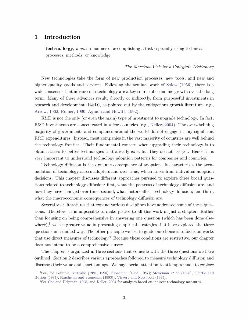
1 Introduction

tech·no·lo·gy, noun: a manner of accomplishing a task especially using technical

processes, methods, or knowledge.

– The Merriam-Webster’s Collegiate Dictionary

New technologies take the form of new production processes, new tools, and new and

higher quality goods and services. Following the seminal work of Solow (1956), there is a

wide consensus that advances in technology are a key source of economic growth over the long

term. Many of these advances result, directly or indirectly, from purposeful investments in

research and development (R&D), as pointed out by the endogenous growth literature (e.g.,

Arrow, 1962, Romer, 1990, Aghion and Howitt, 1992).

R&D is not the only (or even the main) type of investment to upgrade technology. In fact,

R&D investments are concentrated in a few countries (e.g., Keller, 2004). The overwhelming

majority of governments and companies around the world do not engage in any significant

R&D expenditures. Instead, most companies in the vast majority of countries are well behind

the technology frontier. Their fundamental concern when upgrading their technology is to

obtain access to better technologies that already exist but they do not use yet. Hence, it is

very important to understand technology adoption patterns for companies and countries.

Technology diffusion is the dynamic consequence of adoption. It characterizes the accu-

mulation of technology across adopters and over time, which arises from individual adoption

decisions. This chapter discusses different approaches pursued to explore three broad ques-

tions related to technology diffusion: first, what the patterns of technology diffusion are, and

how they have changed over time; second, what factors affect technology diffusion; and third,

what the macroeconomic consequences of technology diffusion are.

Several vast literatures that expand various disciplines have addressed some of these ques-

tions. Therefore, it is impossible to make justice to all this work in just a chapter. Rather

than focusing on being comprehensive in answering one question (which has been done else-

where),1 we see greater value in presenting empirical strategies that have explored the three

questions in a unified way. The other principle we use to guide our choice is to focus on works

that use direct measures of technology.2 Because these conditions are restrictive, our chapter

does not intend to be a comprehensive survey.

The chapter is organized in three sections that coincide with the three questions we have

outlined. Section 2 describes various approaches followed to measure technology diffusion and

discusses their value and shortcomings. We pay special attention to attempts made to explore

1See, for example, Metcalfe (1981, 1998), Stoneman (1983, 1987); Stoneman et al. (1995), Thirtle andRuttan (1987), Karshenas and Stoneman (1993)), Vickery and Northcott (1995).

2See Coe and Helpman, 1995, and Keller, 2004 for analyses based on indirect technology measures.

3

the evolution of adoption patterns over time as well as how they differ across countries. Section

3 explores factors identified as drivers of technology. Section 4 explores the macroeconomic

consequences of technology, focusing mostly on how technology affects income dynamics at

different frequencies. Section 5 concludes with some open questions for future research.

2 Measurement

Prior to studying diffusion patterns, we need to measure technology diffusion. The approaches

developed to measure technology diffusion differ in terms of (i) the dimensions of technology

they intend to measure and (ii) the level at which they try to measure diffusion. In this

section, we describe different existing measures of diffusion, as well as the main lessons from

each approach.

2.1 Extensive measures at the country level

Probably the simplest way to think about technology consists in tracking whether a specific

technology is present or not in a given country at a moment in time. The data requirements

to construct such measures are minimal. Country-level extensive measures are informative of

the overall level of technology in a country if there is large cross-country variation in adoption

lags. However, country-level extensive measures of adoption do not capture how intensively a

technology is used once it is present in the country. As we show below, this condition makes

country-level extensive measures of technology more relevant to study technology adoption

patterns until around the beginning of the twentieth century.

We know from the work of Maddison (2004) that cross-country income differences were

relatively small until the industrial revolution. How large were cross-country differences in

technology adoption in the distant past? Comin et al. (2010) take on this question by as-

sembling three data sets with country-level extensive measures of technology adoption. Each

data set reports the adoption patterns of the inhabitants of modern day territories in differ-

ent historical moments: 1000BC, 0AD and 1500 AD. The first two are coded using twelve

technologies from the “Atlas of Cultural Evolution” (Peregrine, 2003). The data set for 1500

AD covers 24 technologies coded by Comin et al. (2010). The technologies considered satisfy

three criteria. First, they were state of the art technologies (at the time considered); second,

they were used in productive activities (i.e. activities that entered GDP); and third, it has

been possible to document its presence or absence for a wide range of countries. In all three

periods, the technologies can be classified in five broad sectors: agriculture, industry, trans-

portation, communication and military. For each technology, the data set measures whether

it was present (1) or absent (0) from the relevant territory in the relevant period of time.

Comin et al. (2010) compute country-sector adoption levels as the simple average of the bi-

4

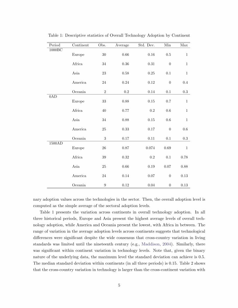
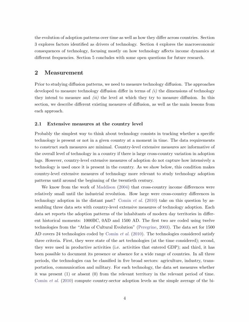
Table 1: Descriptive statistics of Overall Technology Adoption by Continent

Period Continent Obs. Average Std. Dev. Min Max1000BC

Europe 30 0.66 0.16 0.5 1

Africa 34 0.36 0.31 0 1

Asia 23 0.58 0.25 0.1 1

America 24 0.24 0.12 0 0.4

Oceania 2 0.2 0.14 0.1 0.30AD

Europe 33 0.88 0.15 0.7 1

Africa 40 0.77 0.2 0.6 1

Asia 34 0.88 0.15 0.6 1

America 25 0.33 0.17 0 0.6

Oceania 3 0.17 0.11 0.1 0.31500AD

Europe 26 0.87 0.074 0.69 1

Africa 39 0.32 0.2 0.1 0.78

Asia 25 0.66 0.19 0.07 0.88

America 24 0.14 0.07 0 0.13

Oceania 9 0.12 0.04 0 0.13

nary adoption values across the technologies in the sector. Then, the overall adoption level is

computed as the simple average of the sectoral adoption levels.

Table 1 presents the variation across continents in overall technology adoption. In all

three historical periods, Europe and Asia present the highest average levels of overall tech-

nology adoption, while America and Oceania present the lowest, with Africa in between. The

range of variation in the average adoption levels across continents suggests that technological

differences were significant despite the wide consensus that cross-country variation in living

standards was limited until the nineteenth century (e.g., Maddison, 2004). Similarly, there

was significant within continent variation in technology levels. Note that, given the binary

nature of the underlying data, the maximum level the standard deviation can achieve is 0.5.

The median standard deviation within continents (in all three periods) is 0.15. Table 2 shows

that the cross-country variation in technology is larger than the cross-continent variation with

5

Table 2: Variation in technology adoption within countries vs. across countries

STD. of deviations of sectorSTD. across level technology from overall

countries technology adoption within countriesPeriod Obs. Overall Agri. Ind. Military Transp. Comm.

1000BC 114 0.28 0.35 0.18 0.16 0.22 0.23

0 136 0.28 0.25 0.18 0.26 0.24 0.32

1500AD 125 0.32 0.2 0.19 0.13 0.12 0.17

Note: STD. Overall is the cross-country standard deviation in overall technology adoption level.STD. of deviations of sector level technology from overall technology adoption is computed asfollows: σ(xsct−xct) where σ(z) represents the standard deviation of z across countries, xsct is thelevel of technology in sector s, country c, and period t, and xct denotes the overall adoption levelin country c in period t, the average of the adoption levels by sector for country c in period t.

a level for the standard deviation close to 0.3 in all three periods.

Finally, one relevant empirical question is whether all variation in technology is captured

by the variation in the average technology levels in the country or whether there is significant

variation in technology across sectors (within a country). Table 2 explores this question. In

particular, it reports the cross-country dispersion of the deviation between the sectoral and

the overall adoption levels. This dispersion ranges from 0.12 to 0.35 with a median value

of 0.2. These magnitudes suggest that a significant fraction of the variation in technology

adoption is driven by within-country differences in technology across sectors.

2.2 Traditional measures of technology diffusion

It is possible to extend extensive measures of technology diffusion to more disaggregated

levels to study how producers have access to a technology once it has arrived to a country.

Let’s suppose that potential adopters have a binary choice of whether to incur in a sunk cost

of adopting the technology. After they incur in such a cost, they can use the technology

indefinitely at no extra cost. Let’s define Yt as

Yt =mt

M(1)

where M is the (fixed) number of potential adopters and mt is the number of producers that

have adopted the technology at time t. This is how the diffusion literature has measured

diffusion traditionally.

The traditional diffusion literature has fitted S-shaped diffusion curves (like the logistic

function) to diffusion measures such as Yt (Griliches, 1957, Mansfield, 1961, Gort and Klepper,

6

1982). For future reference, the logistic is defined by

Lt =δ1

1 + e−(δ2+δ3t)(2)

where t represents time, δ3 reflects the speed of adoption, δ2 is a constant of integration that

positions the curve on the time scale, and δ1is the long-run outcome.

Several features of this curve are relevant. The logistic curve summarizes the process of

technology diffusion in just three parameters (δ1, δ2 and δ3). It asymptotes to 0 when t goes to

minus infinity and to δ1 when t goes to infinity. Finally, it is symmetric around the inflection

point of Lt = δ1/2 which occurs at t = −δ2/δ3.

Logistic or S-shaped curves have been fitted to technology measures such as (1) for tech-

nologies in many sectors and various countries. Examples of technologies explored in diffusion

studies include the hybrid corn in U.S. states, Griliches (1957), β−blockers in U.S. states, Skin-

ner and Staiger (2007), tetracycline among physicians in four U.S. cities, James S. Coleman

and Menzel (1966), 22 manufacturing processes and machines in the UK (Davies, 1979), and

various consumer durables in the U.S. (Cox and Alm, 1996). The main finding of the tradi-

tional diffusion literature is that S-shaped curves such as (2) provide a good fit to traditional

diffusion measures of the form (1).

The slow initial pace that characterizes logistic diffusion patterns has motivated a number

of theories about the drivers of diffusion.3 Epidemic models (e.g., Griliches, 1957, Mansfield,

1961, 1963, Romeo, 1975, Dixon, 1980, Davies, 1979, Levin et al., 1987 and Rose and Joskow,

1990) build on the premise that the lack of information on the technology prevents potential

adopters from adopting profitable technologies. Information, in turn, is spread slowly because

it only flows from those agents that have already adopted the technology. The so-called probit

model builds on firms’ heterogeneity in adoption costs or profits to generate heterogeneity in

the timing of adoption.4 A third class of models that deliver S-shaped dynamics is based on the

interaction of competition and legitimation forces (Hannan and Freeman, 1989). Legitimation

is the process by which certain types of technologies become accepted as more agents adopt

them. Competition forces limit the maximum level of diffusion as competition for resources

limits the number of agents that an ecosystem can support. Finally, information cascades

are another mechanism that may lead to S-shaped diffusion curves. In Banerjee (1992) and

Arthur (1989), initially, agents may adopt slowly because they are experimenting with various

technological options. After some initial precursors have decided to adopt one technology,

followers may find optimal to copy their predecessors as in a herd leading to an acceleration

of the speed of diffusion.

3See Geroski (2000) for an insightful survey and Skinner and Staiger (2007) for a review of the historicaldiscussion as well as for some evidence to settle it.

4See for example, the vintage human capital of Chari and Hopenhayn (1991) for a beautiful example.

7

Because most studies of technology diffusion that use traditional measures focus on one

single technology and one or a few countries, traditional measures have not been able to shed

light on significant general patterns in technology diffusion. One exception is Cox and Alm

(1996) who show that in the U.S. the time it takes for 25% of potential adopters to adopt a

technology (mostly consumer durables) has declined over the twentieth century.

2.3 The intensive margin

Despite its great intuitive appeal, traditional diffusion measures have two important draw-

backs. First, their computation requires the use micro-level data sets which are hard to

assemble. The limits imposed by this requirement may explain why, after 50 years of re-

search, we still lack comprehensive data sets that cover the diffusion of many technologies, in

many countries over protracted periods. Second, traditional diffusion measures do not capture

the intensity with which each adopter uses the technology.5 For example, a company in the

traditional measure will be coded as an adopter both when only one worker uses the technol-

ogy and when all the workers have access to the technology. Similarly, traditional measures

do not reflect how many units of a given technology a worker uses. Indeed, technological

change is sometimes directed to increasing the number of technological goods that a worker

can use at the same time. These concerns may be significant from a quantitative perspective.

Clark (1987) shows that, circa 1910, the intensity of use of spindles and looms accounted for

the bulk of cross-country productivity differences in cotton mills.

Since micro-level data sets do not tend to collect information on the intensity of use of tech-

nologies, it is difficult to extend traditional diffusion measures to include the intensive margin

of adoption. An alternative approach consists in building these measures using country-level

data. Comin and Hobijn (2004, 2009a) and Comin et al. (2006, 2008a) constructed the CHAT

data set under this premise. CHAT covers the diffusion of 104 technologies (from most sec-

tors of economic activity), for over 150 countries over the last 200 years. The measures of

technology in CHAT are ratios for which the numerator reflect the intensity with which pro-

ducers or consumers employ a technology at a given moment in time and the denominator

scales that by the size of the economy (typically measured by the population or by GDP).

For example, the diffusion of credit and debit cards is measured by the number of credit and

debit card transactions per capita or by the number of points of service per capita, instead

of by the share of people that has at least one credit card. Conceptually, a measure such as

the number of card transactions per capita can be expressed as the product of two variables:

The fraction of people with credit cards, and the average number of transactions of credit

card users per user. The first variable captures the extent of diffusion of credit cards, while

the second captures the intensity with which they are used once they have diffused.

5This is what Mansfield (1968), Davies (1979) and Stoneman (1981) call intra-firm diffusion.

8

Because technology is often embodied in capital goods, some of the measures correspond

to the number of specific capital goods per capita (e.g., computers and telephones). Other

technologies take the form of new production techniques. In these cases, the technology is

measured by the output produced with the technique per capita (e.g., tons of steel produced

with electric arc furnaces per capita). One can make these measures unit free by taking the

logs of the adoption ratios (i.e., log of number of MRI units per capita).

2.3.1 Usage lags

Measures of adoption that incorporate the intensive margin are hard to compare across tech-

nologies because they have different units. This difference in units makes it also difficult to

assess the magnitude of the cross-country variation in technology and its comparison with

cross-country differences in income. Comin et al. (2008b) transform cross-country differences

in adoption intensity to time lags. Time lags have the advantage that they have a common

unit across technologies, (e.g., years). They define the usage lag of technology x in country

c at year t as the answer to the following question: How many years before year t did the

United States last have a usage intensity of technology x that country c has in year t?6

For example, the amount of kWh of electricity (per capita) produced in Uruguay in 1990

was last observed in the United States in 1949. Thus, the electricity usage lag in Uruguay

in 1990 is 41 years. Similarly, the number of personal computers per capita in Spain in 2002

was comparable to that in the United States in 1989. Hence, the 2002 PC usage lag of Spain

is 13 years.

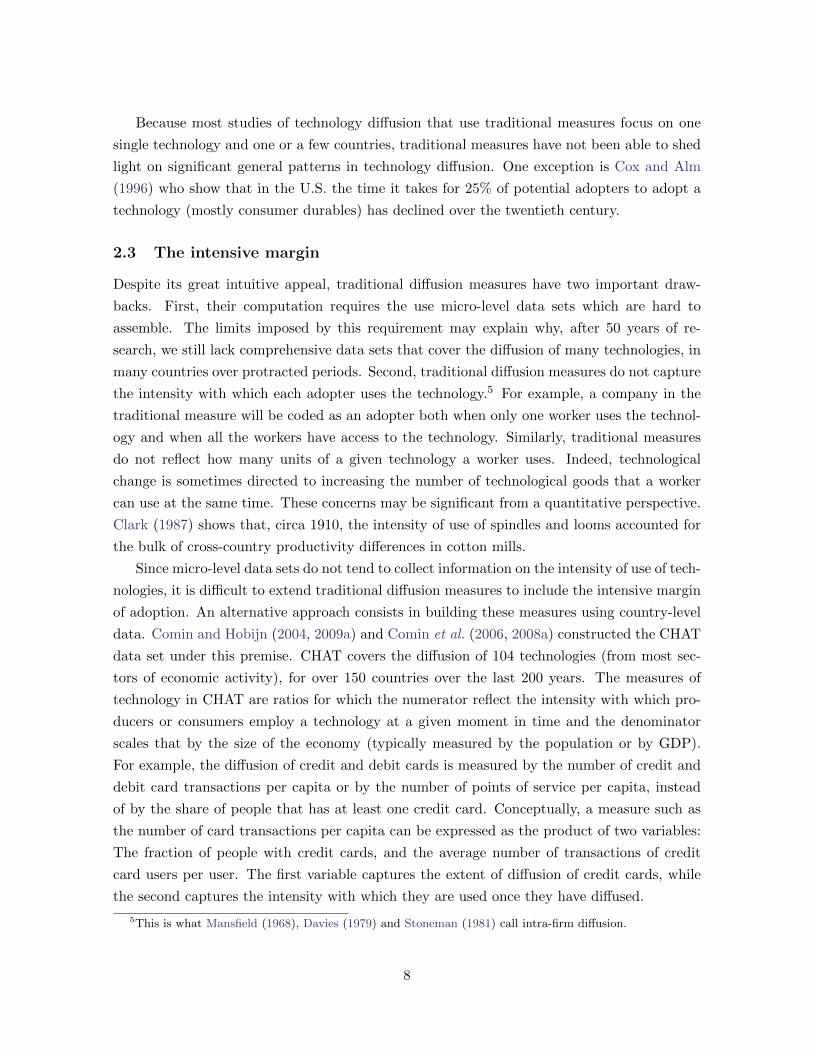
Comin et al. (2008b) compute the usage lags of 10 production technologies in periods

where they are cutting-edge and for which CHAT covers at least 95 countries. These tech-

nologies include electricity production, transportation, communication, IT and agriculture.

In addition, they also compute the time usage lags for per capita GDP. As illustrated by

Figure 1, most of the world population is living in countries with real GDP per capita levels

that have not been observed in the United States in the post World War II era. Moreover,

most of Sub-Saharan Africa, as well as Afghanistan and Mongolia, have per-capita income

levels that have not been observed in the United States since 1820.

With respect to technology usage lags, their main findings are that (i) Technology usage

lags are large, often comparable to lags in real GDP per capita (ii) usage lags are highly

correlated across countries with lags in per-capita income, and (iii) usage lags are highly

correlated across technologies. These results are presented in Table 10) in the Appendix.

6An alternative way to deal with the differences in units is to take logarithms of the technology measures.This is the approach followed by much of the work discussed below.

9

Figure 1: Real GDP per capita lags in year 2000

2.3.2 The shape of diffusion curves once the intensive margin is included

After documenting the magnitude of cross-country differences in technology adoption mea-

sures, one natural question is how do the measures of technology that incorporate the intensive

margin evolve. In particular, do they follow a logistic curve?

Comin et al. (2008a) study this question using an early version of CHAT with 115 tech-

nologies that cover 5,678 technology-country pairs.7 They fit function (2) separately to each

technology-country pair. For 1,291 cases it is not possible to fit the logistic curve due to

the lack of curvature in the data since it covers the late stages of diffusion. For 466 cases,

the estimate of the speed of diffusion (δ3) is negative because the technology has become

obsolete.8

This leaves 3,921 technology-country cases where we can evaluate whether the logistic

7This version of CHAT included some measures of the diffusion of agricultural technologies (typically high-yield seeds) measured as the fraction of agricultural land that used a specific high-yield variety. These seriescame from Evenson and Gollin (2003).

8A negative δ3 can result either from the substitution by a superior technology or because the logistic is apoor fit. To compute how many of the negative estimates of δ3 are due to the former, Comin et al. (2008a)recognize that the presence of competing technologies is likely to have similar effects in the estimates of δ3acrosscountries. Therefore, in those cases where the negative estimate of δ3 is produced by the replacement of adominated technologies, we should observe a large number of negative estimates across countries. Cominet al. (2008a) find that 15 out of 115 technologies considered have negative estimates of δ3 for at least 50%of the technology-country pairs. They identify these as the cases where the estimates of δ3 are driven by theobsolescence of technology, and therefore are cleared from the count. These technologies include open hearthand Bessemer steel production and the number of sail ships, hospital beds, and checks, all of which have beendominated by another technology.

10

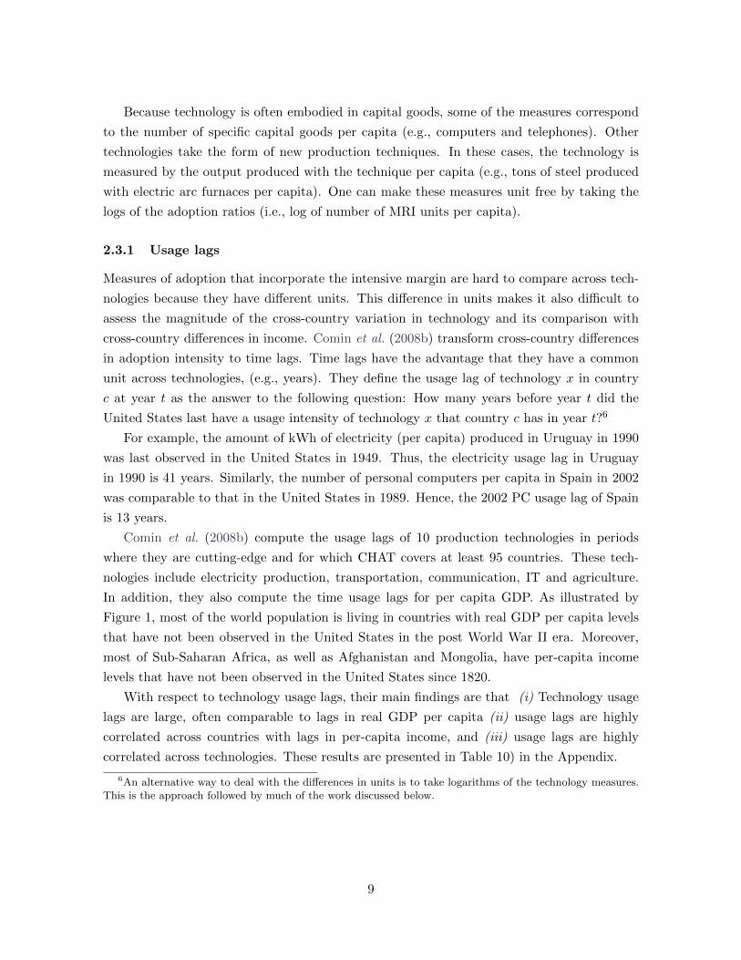
Figure 2: Example of Diffusion Curve

fits well the evolution of technology measures that include the intensive margin of adoption.

For 454 cases, Comin et al. (2008a) still find a negative estimate of δ3 despite not being a

dominated technology. This is, for example, the case of cars per capita in Tanzania, where

population grew faster than the number of cars. For 202 cases, the predicted initial adoption

is previous to the invention date of the technology. For 336 cases, the predicted adoption date

is unrealistically late (either 150 years later that the invention of the technology or 20 years

after the first for the country). Finally, 1,098 cases correspond to technologies that have a

growing ceiling which contradicts the notion that δ1 is fixed.9 Adding these up, it turns out

that for 53% of the technology-country cases (2,084 of 3,921), the logistic does not provide a

good fit to technology diffusion measures that incorporate the intensity of use.

So, if technology measures do not follow a logistic pattern, what do they follow? Figure 2

plots one typical technology measure in CHAT, the production of electricity measured as the

log of MWh produced in the U.S., Japan, Netherlands and Kenya.

There are a number of features worth noting of these curves. First, they have a concave

shape. Second, the shape of these curves is fairly similar. They look as if the same curve,

say the one corresponding to the U.S., had been shifted left and down by different amounts.

These two observations motivate us to conjecture that the curvature of the diffusion curve is

related to technological characteristics common across countries, while horizontal and vertical

shifts of the diffusion curves are informative about cross-country differences. One implication

of this characterization of diffusion curves is that we just need two parameters to characterize

differences across countries in the diffusion of a given technology.

9These include: steam and motor ship tonnage; rail passengers-kilometers; railway freight tonnage; tonsof blast-oxygen furnace, electric-arc furnace, and stainless steel produced; cars; trucks; aviation freight ton-kilometers; TVs; PCs; credit and debit card points of service; ATMs; and checkers.

11

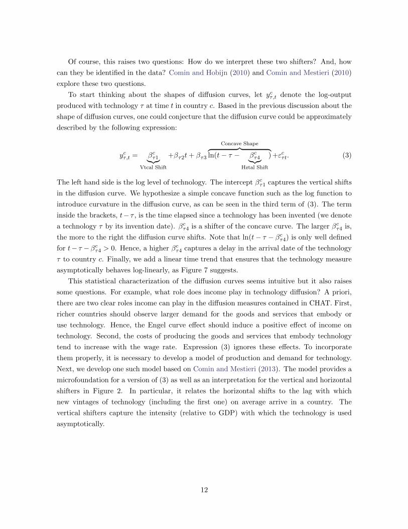
Of course, this raises two questions: How do we interpret these two shifters? And, how

can they be identified in the data? Comin and Hobijn (2010) and Comin and Mestieri (2010)

explore these two questions.

To start thinking about the shapes of diffusion curves, let ycτ ,t denote the log-output

produced with technology τ at time t in country c. Based in the previous discussion about the

shape of diffusion curves, one could conjecture that the diffusion curve could be approximately

described by the following expression:

ycτ ,t = βcτ1︸︷︷︸Vtcal Shift

+βτ2t+ βτ3

Concave Shape︷ ︸︸ ︷ln(t− τ − βcτ4︸︷︷︸

Hztal Shift

) +εcτt. (3)

The left hand side is the log level of technology. The intercept βcτ1 captures the vertical shifts

in the diffusion curve. We hypothesize a simple concave function such as the log function to

introduce curvature in the diffusion curve, as can be seen in the third term of (3). The term

inside the brackets, t− τ , is the time elapsed since a technology has been invented (we denote

a technology τ by its invention date). βcτ4 is a shifter of the concave curve. The larger βcτ4 is,

the more to the right the diffusion curve shifts. Note that ln(t− τ − βcτ4) is only well defined

for t− τ −βcτ4 > 0. Hence, a higher βcτ4 captures a delay in the arrival date of the technology

τ to country c. Finally, we add a linear time trend that ensures that the technology measure

asymptotically behaves log-linearly, as Figure 7 suggests.

This statistical characterization of the diffusion curves seems intuitive but it also raises

some questions. For example, what role does income play in technology diffusion? A priori,

there are two clear roles income can play in the diffusion measures contained in CHAT. First,

richer countries should observe larger demand for the goods and services that embody or

use technology. Hence, the Engel curve effect should induce a positive effect of income on

technology. Second, the costs of producing the goods and services that embody technology

tend to increase with the wage rate. Expression (3) ignores these effects. To incorporate

them properly, it is necessary to develop a model of production and demand for technology.

Next, we develop one such model based on Comin and Mestieri (2013). The model provides a

microfoundation for a version of (3) as well as an interpretation for the vertical and horizontal

shifters in Figure 2. In particular, it relates the horizontal shifts to the lag with which

new vintages of technology (including the first one) on average arrive in a country. The

vertical shifters capture the intensity (relative to GDP) with which the technology is used

asymptotically.

12

2.3.3 A Microfoundation for the Diffusion Curve

Consider the following economic environment. There is a unit measure of identical households

in the economy. Each household supplies inelastically one unit of labor, for which they earn

a wage w. Households can save in domestic bonds which are in zero net supply. The utility

of the representative household is given by

U =

∫ ∞t0

e−ρt ln(Ct)dt (4)

where ρ denotes the discount rate and C, consumption. The representative household, maxi-

mizes its utility subject to the budget constraint (5) and a no-Ponzi scheme condition (6)

Bt + Ct = wt + rtBt, (5)

limt→∞

Bte∫ tt0−rsds ≥ 0, (6)

where B denotes the bond holdings of the representative consumer, B is the increase in bond

holdings over an instant of time, and rt its return on bonds.

World technology frontier.– At a given instant of time, t, the world technology frontier

is characterized by a set of technologies and a set of vintages specific to each technology.

To simplify notation, we omit time subscripts, t, whenever possible. Each instant, a new

technology, τ , exogenously appears. We denote a technology by the time it was invented.

Therefore, the range of invented technologies is (−∞, t].For each existing technology, a new, more productive, vintage appears in the world frontier

every instant. We denote vintages of technology-τ generically by vτ . Vintages are indexed by

the time in which they appear. Thus, the set of existing vintages of technology-τ available

at time t(> τ) is [τ , t]. The productivity of a technology-vintage pair has two components.

The first component, Z(τ , vτ ), is common across countries and it is purely determined by

technological attributes. In particular,

Z(τ , v) = e(χ+γ)τ+γ(vτ−τ) (7)

= eχτ+γvτ , (8)

where (χ+ γ)τ is the productivity level associated with the first vintage of technology τ and

γ(vτ − τ) captures the productivity gains associated with the introduction of new vintages

(vτ ≥ τ).10

The second component is a technology-country specific productivity term, aτ , which we

10In what follows, whenever there is no confusion, we omit the subscript τ from the vintage notation andsimply write v.

13

further discuss below.

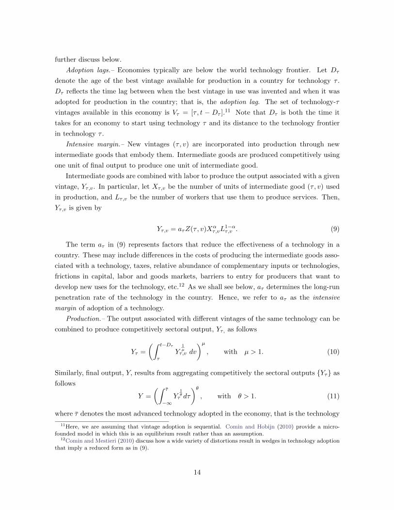
Adoption lags.– Economies typically are below the world technology frontier. Let Dτ

denote the age of the best vintage available for production in a country for technology τ .

Dτ reflects the time lag between when the best vintage in use was invented and when it was

adopted for production in the country; that is, the adoption lag. The set of technology-τ

vintages available in this economy is Vτ = [τ , t − Dτ ].11 Note that Dτ is both the time it

takes for an economy to start using technology τ and its distance to the technology frontier

in technology τ .

Intensive margin.– New vintages (τ , v) are incorporated into production through new

intermediate goods that embody them. Intermediate goods are produced competitively using

one unit of final output to produce one unit of intermediate good.

Intermediate goods are combined with labor to produce the output associated with a given

vintage, Yτ ,v. In particular, let Xτ ,v be the number of units of intermediate good (τ , v) used

in production, and Lτ ,v be the number of workers that use them to produce services. Then,

Yτ ,v is given by

Yτ ,v = aτZ(τ , v)Xατ,vL

1−ατ,v . (9)

The term aτ in (9) represents factors that reduce the effectiveness of a technology in a

country. These may include differences in the costs of producing the intermediate goods asso-

ciated with a technology, taxes, relative abundance of complementary inputs or technologies,

frictions in capital, labor and goods markets, barriers to entry for producers that want to

develop new uses for the technology, etc.12 As we shall see below, aτ determines the long-run

penetration rate of the technology in the country. Hence, we refer to aτ as the intensive

margin of adoption of a technology.

Production.– The output associated with different vintages of the same technology can be

combined to produce competitively sectoral output, Yτ , as follows

Yτ =

(∫ t−Dτ

τY

1µτ ,v dv

)µ, with µ > 1. (10)

Similarly, final output, Y, results from aggregating competitively the sectoral outputs {Yτ} as

follows

Y =

(∫ τ

−∞Y

1θτ dτ

)θ, with θ > 1. (11)

where τ denotes the most advanced technology adopted in the economy, that is the technology

11Here, we are assuming that vintage adoption is sequential. Comin and Hobijn (2010) provide a micro-founded model in which this is an equilibrium result rather than an assumption.

12Comin and Mestieri (2010) discuss how a wide variety of distortions result in wedges in technology adoptionthat imply a reduced form as in (9).

14

τ for which τ = t−Dτ .

Factor Demands and Final Output

We take the price of final output as numeraire. The demand for output produced with a

particular technology is

Yτ = Y p− θθ−1

τ (12)

where pτ is the price of sector τ output. Both the income level of a country and the price of

a technology affect the demand of output produced with a given technology. Because of the

homotheticity of the production function, the income elasticity of technology τ output is one.

Similarly, the demand for output produced with a particular technology vintage is

Yτ ,v = Yτ

(pτpτ ,v

)− µµ−1

, (13)

where pτ ,v denotes the price of the (τ , v) intermediate good.13 The demands for labor and

intermediate goods at the vintage level are

(1− α)pτ ,vYτ ,vLτ ,v

= w (14)

αpτ ,vYτ ,vXτ ,v

= 1 (15)

Perfect competition in the production of intermediate goods implies that the price of

intermediate goods equals their marginal cost,

pτ ,v =w1−α

Z(τ , v)aτ(1− α)−(1−α)α−α (16)

Combining (13), (14) and (15), the total output produced with technology τ can be ex-

pressed as

Yτ = ZτL1−ατ Xα

τ , (17)

where Lτ denotes the total labor used in sector τ ,

Lτ =

∫ t−Dτ

τLτ ,vdv, (18)

Xτ is the total amount of intermediate goods in sector τ ,

Xτ =

∫ t−Dτ

τXτ ,vdv, (19)

13Even though older technology-vintage pairs are always produced in equilibrium, the value of its productionrelative to total output is declining over time.

15

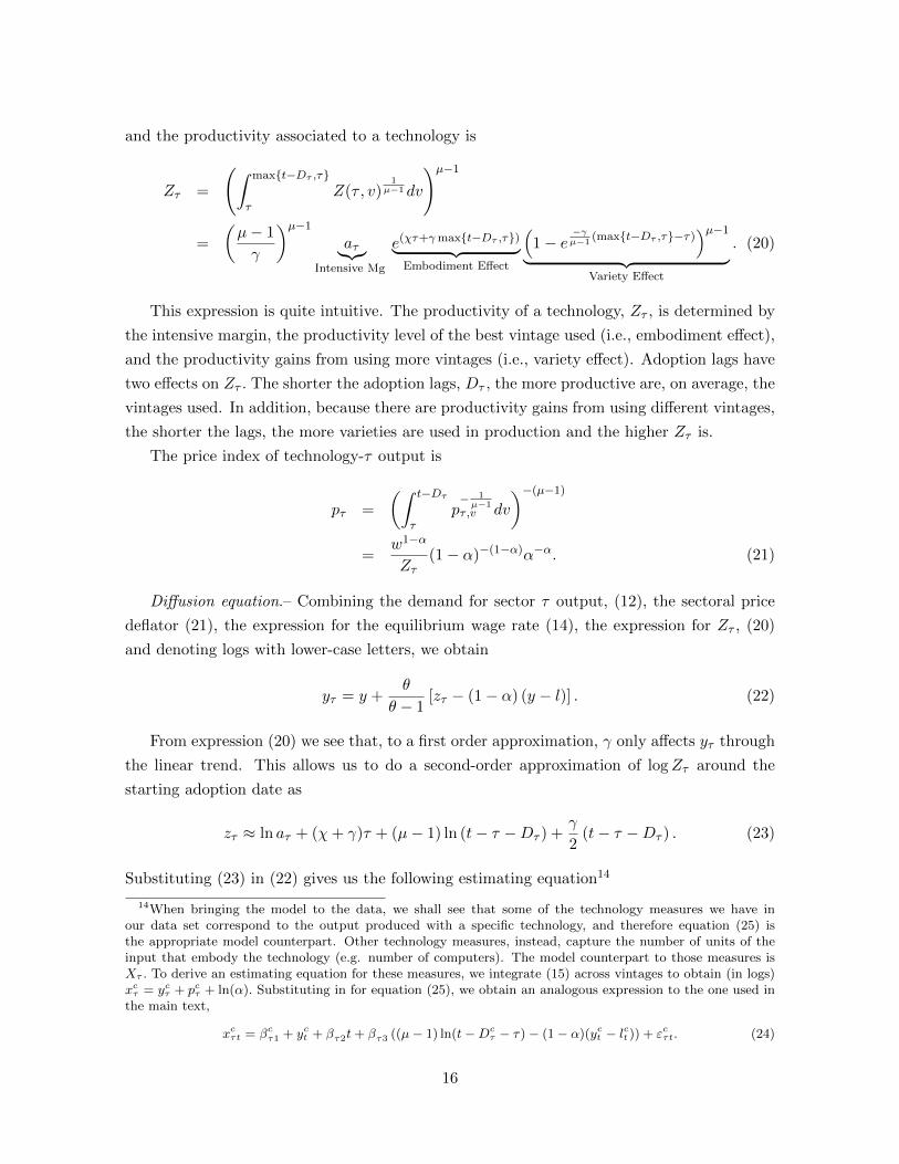
and the productivity associated to a technology is

Zτ =

(∫ max{t−Dτ ,τ}

τZ(τ , v)

1µ−1dv

)µ−1

=

(µ− 1

γ

)µ−1

aτ︸︷︷︸Intensive Mg

e(χτ+γmax{t−Dτ ,τ})︸ ︷︷ ︸Embodiment Effect

(1− e

−γµ−1

(max{t−Dτ ,τ}−τ))µ−1

︸ ︷︷ ︸Variety Effect

. (20)

This expression is quite intuitive. The productivity of a technology, Zτ , is determined by

the intensive margin, the productivity level of the best vintage used (i.e., embodiment effect),

and the productivity gains from using more vintages (i.e., variety effect). Adoption lags have

two effects on Zτ . The shorter the adoption lags, Dτ , the more productive are, on average, the

vintages used. In addition, because there are productivity gains from using different vintages,

the shorter the lags, the more varieties are used in production and the higher Zτ is.

The price index of technology-τ output is

pτ =

(∫ t−Dτ

τp− 1µ−1

τ ,v dv

)−(µ−1)

=w1−α

Zτ(1− α)−(1−α)α−α. (21)

Diffusion equation.– Combining the demand for sector τ output, (12), the sectoral price

deflator (21), the expression for the equilibrium wage rate (14), the expression for Zτ , (20)

and denoting logs with lower-case letters, we obtain

yτ = y +θ

θ − 1[zτ − (1− α) (y − l)] . (22)

From expression (20) we see that, to a first order approximation, γ only affects yτ through

the linear trend. This allows us to do a second-order approximation of logZτ around the

starting adoption date as

zτ ≈ ln aτ + (χ+ γ)τ + (µ− 1) ln (t− τ −Dτ ) +γ

2(t− τ −Dτ ) . (23)

Substituting (23) in (22) gives us the following estimating equation14

14When bringing the model to the data, we shall see that some of the technology measures we have inour data set correspond to the output produced with a specific technology, and therefore equation (25) isthe appropriate model counterpart. Other technology measures, instead, capture the number of units of theinput that embody the technology (e.g. number of computers). The model counterpart to those measures isXτ . To derive an estimating equation for these measures, we integrate (15) across vintages to obtain (in logs)xcτ = ycτ + pcτ + ln(α). Substituting in for equation (25), we obtain an analogous expression to the one used inthe main text,

xcτt = βcτ1 + yct + βτ2t+ βτ3 ((µ− 1) ln(t−Dcτ − τ)− (1− α)(yct − lct )) + εcτt. (24)

16

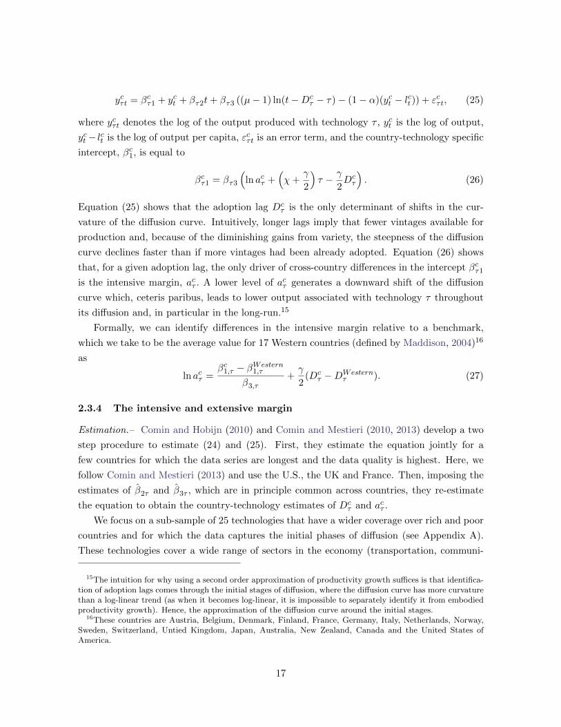
ycτt = βcτ1 + yct + βτ2t+ βτ3 ((µ− 1) ln(t−Dcτ − τ)− (1− α)(yct − lct )) + εcτt, (25)

where ycτt denotes the log of the output produced with technology τ , yct is the log of output,

yct − lct is the log of output per capita, εcτt is an error term, and the country-technology specific

intercept, βc1, is equal to

βcτ1 = βτ3

(ln acτ +

(χ+

γ

2

)τ − γ

2Dcτ

). (26)

Equation (25) shows that the adoption lag Dcτ is the only determinant of shifts in the cur-

vature of the diffusion curve. Intuitively, longer lags imply that fewer vintages available for

production and, because of the diminishing gains from variety, the steepness of the diffusion

curve declines faster than if more vintages had been already adopted. Equation (26) shows

that, for a given adoption lag, the only driver of cross-country differences in the intercept βcτ1

is the intensive margin, acτ . A lower level of acτ generates a downward shift of the diffusion

curve which, ceteris paribus, leads to lower output associated with technology τ throughout

its diffusion and, in particular in the long-run.15

Formally, we can identify differences in the intensive margin relative to a benchmark,

which we take to be the average value for 17 Western countries (defined by Maddison, 2004)16

as

ln acτ =βc1,τ − βWestern

1,τ

β3,τ

+γ

2(Dc

τ −DWesternτ ). (27)

2.3.4 The intensive and extensive margin

Estimation.– Comin and Hobijn (2010) and Comin and Mestieri (2010, 2013) develop a two

step procedure to estimate (24) and (25). First, they estimate the equation jointly for a

few countries for which the data series are longest and the data quality is highest. Here, we

follow Comin and Mestieri (2013) and use the U.S., the UK and France. Then, imposing the

estimates of β2τ and β3τ , which are in principle common across countries, they re-estimate

the equation to obtain the country-technology estimates of Dcτ and acτ .

We focus on a sub-sample of 25 technologies that have a wider coverage over rich and poor

countries and for which the data captures the initial phases of diffusion (see Appendix A).

These technologies cover a wide range of sectors in the economy (transportation, communi-

15The intuition for why using a second order approximation of productivity growth suffices is that identifica-tion of adoption lags comes through the initial stages of diffusion, where the diffusion curve has more curvaturethan a log-linear trend (as when it becomes log-linear, it is impossible to separately identify it from embodiedproductivity growth). Hence, the approximation of the diffusion curve around the initial stages.

16These countries are Austria, Belgium, Denmark, Finland, France, Germany, Italy, Netherlands, Norway,Sweden, Switzerland, Untied Kingdom, Japan, Australia, New Zealand, Canada and the United States ofAmerica.

17

cation and IT, industrial, agricultural and medical sectors). Their invention dates also span

quite evenly over the last 200 years.

As in Comin and Hobijn (2010), we use the plausibility and precision of the estimates

of the adoption lags from equation (25) as a pre-requisite to utilize the technology-country

pair in our analysis. We find that these two conditions are met for the majority of the

technology country-pairs (67%).17 For these technology country-pairs, we find that equation

(25) provides a very good fit for the data with an average detrended R2 of 0.79 across countries

and technologies (Table 11).18

Statistics.–Tables 3 and 4 report summary statistics for the estimates of the adoption lags

and the intensive margin for each technology. The average adoption lag across all technologies

(and countries) is 44 years. We find significant variation in average adoption lags across tech-

nologies. The range goes from 7 years for the Internet to 121 years for steam and motor ships.

There is also considerable cross-country variation in adoption lags for any given technology.

The range for the cross-country standard deviations goes from 3 years for PCs to 53 years for

steam and motor ships.

We also find significant cross-country variation in the intensive margin. The intensive

margin is reported as log differences relative to the average adoption of Western countries.19

The average intensive margin is -0.62, which implies that the level of adoption of the average

country is 54% of the Western countries. More generally, there is significant cross-country

dispersion in the intensive margin. The range goes from 0.3 for mail to 1.1 for cars and the

Internet. These summary statistics for the estimates of adoption lags and the intensive margin

of adoption are consistent with those in Comin and Hobijn (2010) and Comin and Mestieri

(2010) which use smaller technology samples and estimate other versions of the diffusion

equation (25).

Evolution.– The long-time spans and cross-country coverage of the technologies in CHAT

allow us to explore the presence of cross-country trends in adoption patterns. Comin and

Hobijn (2010) explored whether there has been any trend in adoption lags over the last 200

years. They find that the average lag with which countries adopt technologies has dropped

17Plausible adoption lags are those with an estimated adoption date of no less than ten years before theinvention date (this is to allow for some inference error). Precise are those with a significant estimate ofadoption lags and the intercept βc1τ at a 5% level. Following Comin and Hobijn (2010), we relax this conditionand include in the “precise” category those estimates that have a standard error of adoption lags smaller than√

2003− invention date. The idea is to allow for some older technologies to be more imprecisely estimated.However, this additional margin hardly expands the set of precise estimates. Only 15 additional estimatesare included with this condition, which represent 1.2% of our precise observations. Most of the implausibleestimates correspond to diffusion curves that do not have the initial phases of diffusion. This makes it veryhard to separately identify the log-linear trend from the log component of (25).

18To compute the detrended R2, we partial out the linear trend γt and compute the R2 of the detrendeddata.

19To compute the intensive margin we follow Comin and Mestieri (2013) and calibrate γ = (1 − α) · 1%,α = 0.3, and use a value of β3,τ that results from setting the elasticity across technologies θ to be the meanacross our estimates, which is θ = 1.28.

18

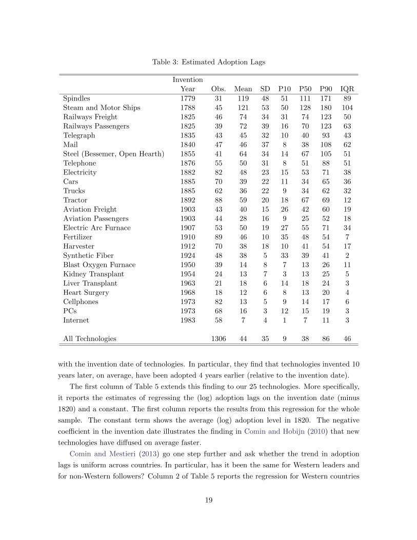
Table 3: Estimated Adoption Lags

InventionYear Obs. Mean SD P10 P50 P90 IQR

Spindles 1779 31 119 48 51 111 171 89Steam and Motor Ships 1788 45 121 53 50 128 180 104Railways Freight 1825 46 74 34 31 74 123 50Railways Passengers 1825 39 72 39 16 70 123 63Telegraph 1835 43 45 32 10 40 93 43Mail 1840 47 46 37 8 38 108 62Steel (Bessemer, Open Hearth) 1855 41 64 34 14 67 105 51Telephone 1876 55 50 31 8 51 88 51Electricity 1882 82 48 23 15 53 71 38Cars 1885 70 39 22 11 34 65 36Trucks 1885 62 36 22 9 34 62 32Tractor 1892 88 59 20 18 67 69 12Aviation Freight 1903 43 40 15 26 42 60 19Aviation Passengers 1903 44 28 16 9 25 52 18Electric Arc Furnace 1907 53 50 19 27 55 71 34Fertilizer 1910 89 46 10 35 48 54 7Harvester 1912 70 38 18 10 41 54 17Synthetic Fiber 1924 48 38 5 33 39 41 2Blast Oxygen Furnace 1950 39 14 8 7 13 26 11Kidney Transplant 1954 24 13 7 3 13 25 5Liver Transplant 1963 21 18 6 14 18 24 3Heart Surgery 1968 18 12 6 8 13 20 4Cellphones 1973 82 13 5 9 14 17 6PCs 1973 68 16 3 12 15 19 3Internet 1983 58 7 4 1 7 11 3

All Technologies 1306 44 35 9 38 86 46

with the invention date of technologies. In particular, they find that technologies invented 10

years later, on average, have been adopted 4 years earlier (relative to the invention date).

The first column of Table 5 extends this finding to our 25 technologies. More specifically,

it reports the estimates of regressing the (log) adoption lags on the invention date (minus

1820) and a constant. The first column reports the results from this regression for the whole

sample. The constant term shows the average (log) adoption level in 1820. The negative

coefficient in the invention date illustrates the finding in Comin and Hobijn (2010) that new

technologies have diffused on average faster.

Comin and Mestieri (2013) go one step further and ask whether the trend in adoption

lags is uniform across countries. In particular, has it been the same for Western leaders and

for non-Western followers? Column 2 of Table 5 reports the regression for Western countries

19

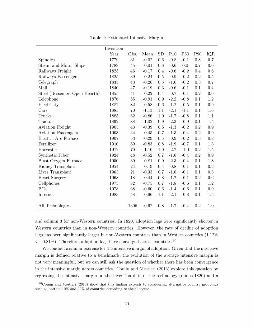
Table 4: Estimated Intensive Margin

InventionYear Obs. Mean SD P10 P50 P90 IQR

Spindles 1779 31 -0.02 0.6 -0.8 -0.1 0.8 0.7Steam and Motor Ships 1788 45 -0.01 0.6 -0.6 0.0 0.7 0.6Railways Freight 1825 46 -0.17 0.4 -0.6 -0.2 0.4 0.6Railways Passengers 1825 39 -0.24 0.5 -0.9 -0.2 0.2 0.5Telegraph 1835 43 -0.26 0.5 -1.0 -0.2 0.3 0.7Mail 1840 47 -0.19 0.3 -0.6 -0.1 0.1 0.4Steel (Bessemer, Open Hearth) 1855 41 -0.22 0.4 -0.7 -0.1 0.2 0.6Telephone 1876 55 -0.91 0.9 -2.2 -0.8 0.1 1.2Electricity 1882 82 -0.58 0.6 -1.2 -0.5 0.1 0.9Cars 1885 70 -1.13 1.1 -2.1 -1.1 0.1 1.6Trucks 1885 62 -0.86 1.0 -1.7 -0.8 0.1 1.1Tractor 1892 88 -1.02 0.9 -2.3 -0.9 0.1 1.5Aviation Freight 1903 43 -0.39 0.6 -1.3 -0.2 0.2 0.9Aviation Passengers 1903 44 -0.45 0.7 -1.3 -0.4 0.2 0.9Electric Arc Furnace 1907 53 -0.29 0.5 -0.9 -0.2 0.3 0.8Fertilizer 1910 89 -0.83 0.8 -1.9 -0.7 0.1 1.3Harvester 1912 70 -1.10 1.0 -2.7 -1.0 0.2 1.5Synthetic Fiber 1924 48 -0.52 0.7 -1.6 -0.4 0.2 0.9Blast Oxygen Furnace 1950 39 -0.81 0.9 -2.3 -0.4 0.1 1.8Kidney Transplant 1954 24 -0.19 0.4 -0.8 -0.1 0.1 0.3Liver Transplant 1963 21 -0.33 0.7 -1.6 -0.1 0.1 0.5Heart Surgery 1968 18 -0.44 0.8 -1.7 -0.1 0.2 0.6Cellphones 1973 82 -0.75 0.7 -1.8 -0.6 0.1 1.2PCs 1973 68 -0.60 0.6 -1.4 -0.6 0.1 0.9Internet 1983 58 -0.96 1.1 -2.1 -0.8 0.1 1.5

All Technologies 1306 -0.62 0.8 -1.7 -0.4 0.2 1.0

and column 3 for non-Western countries. In 1820, adoption lags were significantly shorter in

Western countries than in non-Western countries. However, the rate of decline of adoption

lags has been significantly larger in non-Western countries than in Western countries (1.12%

vs. 0.81%). Therefore, adoption lags have converged across countries.20

We conduct a similar exercise for the intensive margin of adoption. Given that the intensive

margin is defined relative to a benchmark, the evolution of the average intensive margin is

not very meaningful, but we can still ask the question of whether there has been convergence

in the intensive margin across countries. Comin and Mestieri (2013) explore this question by

regressing the intensive margin on the invention date of the technology (minus 1820) and a

20Comin and Mestieri (2013) show that this finding extends to considering alternative country groupingssuch as bottom 10% and 20% of countries according to their income.

20

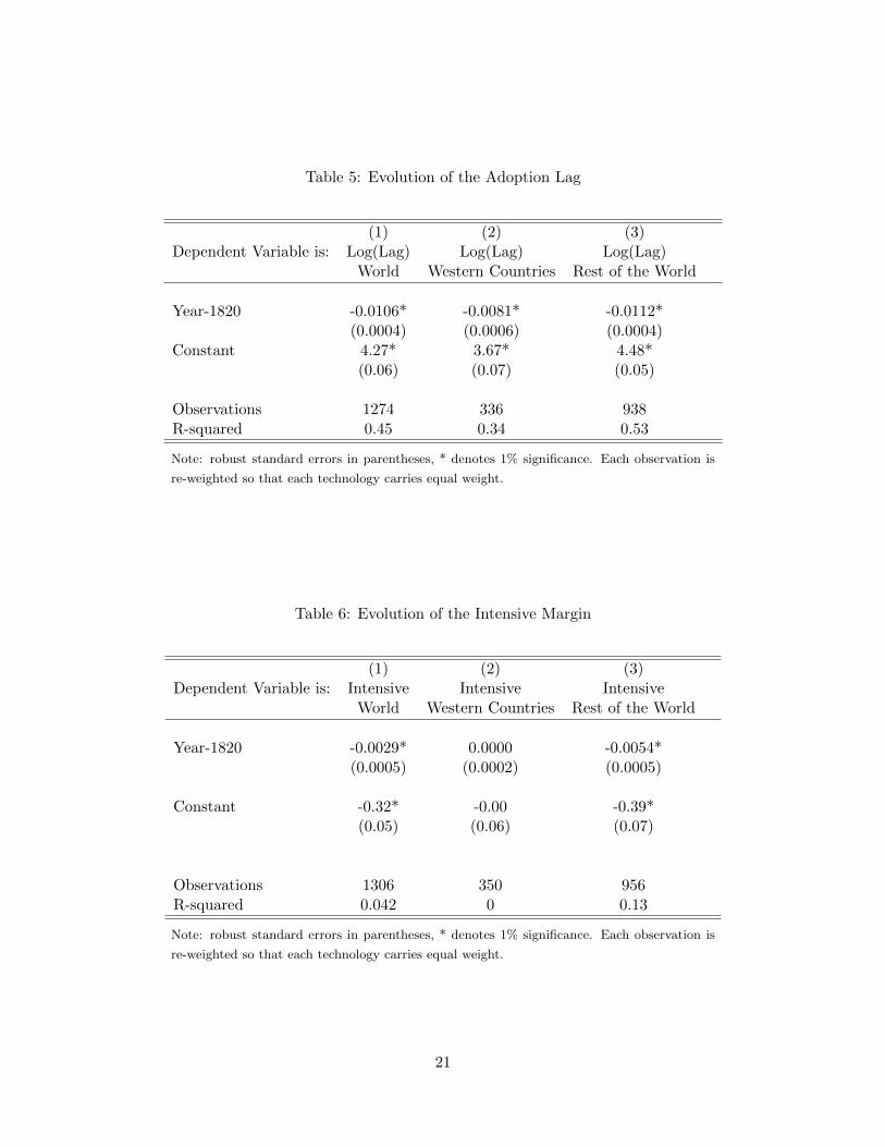
Table 5: Evolution of the Adoption Lag

(1) (2) (3)Dependent Variable is: Log(Lag) Log(Lag) Log(Lag)

World Western Countries Rest of the World

Year-1820 -0.0106* -0.0081* -0.0112*(0.0004) (0.0006) (0.0004)

Constant 4.27* 3.67* 4.48*(0.06) (0.07) (0.05)

Observations 1274 336 938R-squared 0.45 0.34 0.53

Note: robust standard errors in parentheses, * denotes 1% significance. Each observation is

re-weighted so that each technology carries equal weight.

Table 6: Evolution of the Intensive Margin

(1) (2) (3)Dependent Variable is: Intensive Intensive Intensive

World Western Countries Rest of the World

Year-1820 -0.0029* 0.0000 -0.0054*(0.0005) (0.0002) (0.0005)

Constant -0.32* -0.00 -0.39*(0.05) (0.06) (0.07)

Observations 1306 350 956R-squared 0.042 0 0.13

Note: robust standard errors in parentheses, * denotes 1% significance. Each observation is

re-weighted so that each technology carries equal weight.

21

constant. Table 6 reports their main finding. As shown in column 3, the intensive margin in

non-Western countries (relative to the Western average) has declined (with the invention date)

at a rate of 0.54% per year. This estimate implies that the gap in the intensity of technology

adoption between rich and poor countries is larger for newer than for old technologies. So,

there has been divergence in the intensive margin over the last 200 years. In Section (4.3) we

review the implications that this has had on the cross-country dynamics of income.

Robustness checks.– One important identification assumption is that the curvature of the

diffusion curve (25), β3τ , is common across countries for a given technology τ . Comin and

Hobijn (2010) evaluate this hypothesis by allowing it to vary by technology country pair and

then testing the null that the common and the country-specific estimate of β3τ are the same.

Reassuringly, they find that they cannot reject the null that both estimates are the same for

69% of the technology-country pairs.

A second restriction used in the estimation –this one imposed by the model – is that the

elasticity of technology with respect to income is one. The homotheticity of technology may

be a restrictive constraint in reality. To evaluate the robustness of the findings to alternative

formulations of the demand for technology, Comin and Mestieri (2013) propose a method to

estimate the income elasticity of technology. Specifically, they estimate the income elasticity of

technology in the first stage (along with β2 and β3) for the three baseline countries (U.S., UK

and France). Effectively, this implies that the income elasticity of technology is identified from

the time-series variation of technology and income for these countries. Since the time-span

of the diffusion for most technologies in these countries is quite long, it covers periods when

their income was far lower than today. Hence, this estimate seems a reasonable proxy for the

income elasticity of technology in developing countries too. They find that both the estimates

and the trends in adoption described above are robust to allowing for non-homotheticities in

demand.

2.4 Other Approaches

We conclude our discussion of the measurement of technology by mentioning one recent ap-

proach proposed by Alexopoulos (2011). Her approach consists in measuring technology by

the number of books published in the field of a particular technology. The rationale of this

measure is that technology books are published when new discoveries (relevant for the indus-

try) are made. One advantage of this measure is that, because the topics covered by books

are classified into narrow fields, it is possible to collect time-series measures for relatively

disaggregated fields.

One important question is whether these measures capture innovations or diffusion of

the innovations. To explore this issue, Alexopoulos shows that the number of new books

on a given technological field peak in the early stages of diffusion of a new technology, and

22

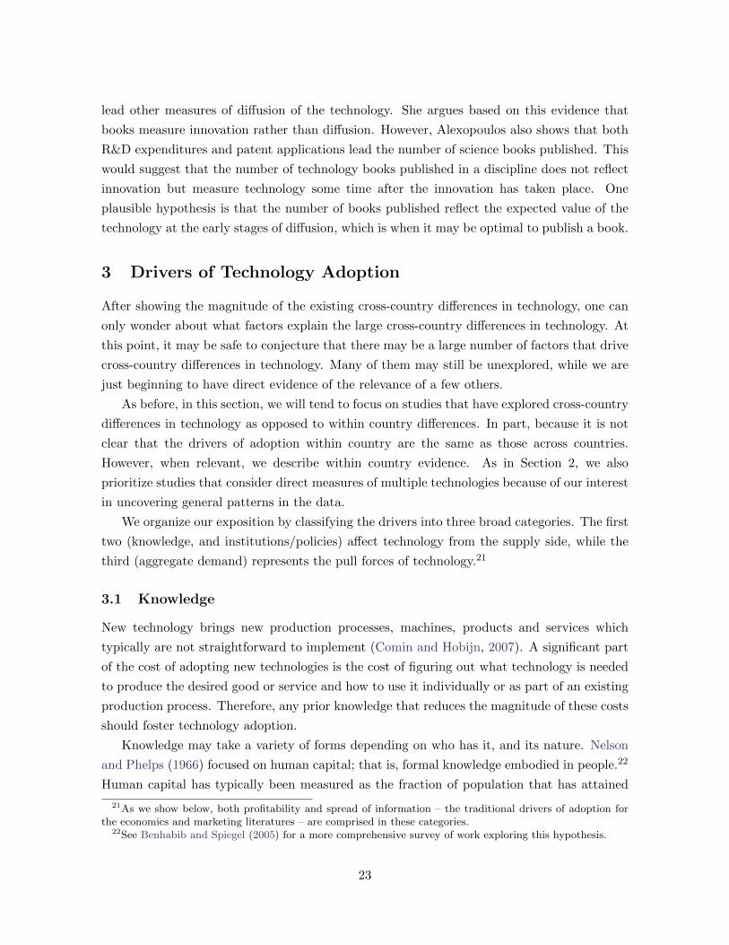
lead other measures of diffusion of the technology. She argues based on this evidence that

books measure innovation rather than diffusion. However, Alexopoulos also shows that both

R&D expenditures and patent applications lead the number of science books published. This

would suggest that the number of technology books published in a discipline does not reflect

innovation but measure technology some time after the innovation has taken place. One

plausible hypothesis is that the number of books published reflect the expected value of the

technology at the early stages of diffusion, which is when it may be optimal to publish a book.

3 Drivers of Technology Adoption

After showing the magnitude of the existing cross-country differences in technology, one can

only wonder about what factors explain the large cross-country differences in technology. At

this point, it may be safe to conjecture that there may be a large number of factors that drive

cross-country differences in technology. Many of them may still be unexplored, while we are

just beginning to have direct evidence of the relevance of a few others.

As before, in this section, we will tend to focus on studies that have explored cross-country

differences in technology as opposed to within country differences. In part, because it is not

clear that the drivers of adoption within country are the same as those across countries.

However, when relevant, we describe within country evidence. As in Section 2, we also

prioritize studies that consider direct measures of multiple technologies because of our interest

in uncovering general patterns in the data.

We organize our exposition by classifying the drivers into three broad categories. The first

two (knowledge, and institutions/policies) affect technology from the supply side, while the

third (aggregate demand) represents the pull forces of technology.21

3.1 Knowledge

New technology brings new production processes, machines, products and services which

typically are not straightforward to implement (Comin and Hobijn, 2007). A significant part

of the cost of adopting new technologies is the cost of figuring out what technology is needed

to produce the desired good or service and how to use it individually or as part of an existing

production process. Therefore, any prior knowledge that reduces the magnitude of these costs

should foster technology adoption.

Knowledge may take a variety of forms depending on who has it, and its nature. Nelson

and Phelps (1966) focused on human capital; that is, formal knowledge embodied in people.22

Human capital has typically been measured as the fraction of population that has attained

21As we show below, both profitability and spread of information – the traditional drivers of adoption forthe economics and marketing literatures – are comprised in these categories.

22See Benhabib and Spiegel (2005) for a more comprehensive survey of work exploring this hypothesis.

23

a certain schooling level or as the fraction of population in schooling age that is enrolled in

certain schooling level. Formal schooling may not be the only (or even the most relevant)

source of knowledge for the adoption of new technologies since workers may learn on the job.23

In addition to knowledge embodied in people, knowledge may be collectively embodied in

organizations or in sectors. The concept of organizational knowledge captures the notion that

there may be complementarities between the knowledge of workers which increase the organi-

zation capacity to adopt new technologies beyond the sum of the workers individual capacities.

Finally, a company’s capabilities to adopt or use a new technology may be positively affected

by the capabilities of other agents. These may be similar companies in the same geography

(clusters), e.g., Porter (1998), or distinct organizations with which it interacts directly or indi-

rectly. For example, a company may seek technological advice from public organizations that

have prior experience in the technology (e.g., Fraunhofer in Germany, Comin et al., 2012).

Finally, a company’s adoption potential may be affected by the technological experience of

companies in other geographies with which it has some contact. This implication would follow

from a simple extension of epidemic diffusion models (to allow for multiple geographies).

Next, we review some evidence about the role of the different sources of knowledge on

technology adoption.

3.1.1 Human capital

Caselli and Coleman (2001) explore the role of human capital in the diffusion of comput-

ers. Using data on the value of computer imports for 90 countries between 1970 and 1990,

they study whether imports are affected by various measures of human capital. In their

specification, they control for per-capita income, year-dummies, continent dummies and a

country-level random effect. They find that an increase by one percentage point in the frac-

tion of the population with more than primary schooling is associated with an increase in the

value of computers imported by one percent.

Riddell and Song (2012) use Canadian micro-level data from the Workplace and Employee

Survey to explore the same question. More specifically, these authors use time and state vari-

ation in compulsory education laws to instrument the education attainment of workers. Their

main findings are that graduating from high-school increases the probability of using a com-

puter in the job by 37 percentage points. Similarly, an additional year of schooling increases

this probability by 7 percentage points. In contrast, they do not find any significant effect

of education on the probability that a worker uses computer-controlled machines. There are

a few remarks worth making about the findings in Riddell and Song (2012). First, the fact

that a worker’s own human capital does not affect his probability of adopting numerically

controlled machines does not imply that human capital is irrelevant for the diffusion of this

23See for example Seshadri and Manuelli (2005), Erosa et al. (2010) and the references therein.

24

technology. It may well be the case that the human capital of other relevant agents is im-

portant (technicians, managers, importers,. . . ). A second remark made by Riddell and Song

concerns the significantly higher estimates (almost three times) for the effect of human capi-

tal on computer adoption when instrumenting education than with OLS. This result suggests

that, with the instrumentation, the authors are probably capturing the local average treat-

ment effect (LATE) rather than the average treatment effect (ATE) which is the relevant

measure for the question posed.

One would like to explore whether the importance of human capital for technology adop-

tion extends beyond computers. Benhabib and Spiegel (1994) find evidence that the stock

of human capital affects the growth rate of productivity (i.e., TFP) which they interpret in

the light of the Nelson and Phelps (1966) model. Comin and Hobijn (2004) look at the pre-

decessor of CHAT (the HCCTAD) which contains information on the diffusion of 25 major

technologies in 15 advanced countries over the last 200 years.

The specification used by Comin and Hobijn (2004) is similar to the one used by Caselli

and Coleman (2001). In particular, they consider the following regression:

ycjt = ηjt + βXcjt + εcjt (28)

where ycjt denotes the adoption level of technology j in country c in year t, ηjt is a full set

of technology-time dummies, and Xcjt is a matrix of (possibly technology specific) controls.

In particular Xcjt always include the log of GDP per capita and may include controls for the

openness of the country, quality of political institutions, measures of adoption of general tech-

nologies (i.e., electricity) and of predecessor technologies. The regression results are reported

in Table 7.

Because of data constraints, Comin and Hobijn (2004) allow for different effects of enroll-

ment rates before and after 1970. The most robust result they find concerning human capital

is that, until 1970, secondary enrollment is positively associated with technology adoption.

This effect does not diminish after including all these controls with the exception of electric-

ity production and the predecessor technologies which reduces significantly the sample (from

over 5000 to 1000 observations) and reduces the regression coefficient by a fourth (from 0.3

to 0.22). After 1970, however, they find no significant effect of secondary enrollment on tech-

nology adoption. Attainment rates (in all schooling level) are also positively associated with

technology adoption.

Comin and Hobijn (2004) also explore the association between education and adoption

of specific technologies. Consistent with Riddell and Song (2012), they find heterogeneity in

the coefficients. The positive impact of secondary schooling on adoption is driven by mass

communication technologies (newspapers, radio and TV) and by electricity. For the other

technologies the association with secondary enrollment is insignificant. For transportation

25

Table 7: Technology Pooled Regressions

Dependent Variable is: Technologycjtln(RGDPpc) 1.15 1.12 0.57 1.10 1.05 0.93 1.04 1.04 1.2

(0.03)* (0.03)* 0 (0.07)* (0.03)* (0.04)* (0.05)* (0.35)* (0.03)* (0.09)*

Prim.enr. 70- 0.09 0.06 0.08 1.23 0.10 0.09 1.69(0.06) (0.07) (0.07) (0.18)* (0.07) (0.07) (0.26)*

Prim enr. 70+ 0.35 0.39 0.22 -0.11 -0.48(0.21) (0.23) (0.23) (0.2) (0.4)

Sec.enr. 70- 0.30 0.36 0.31 0.37 0.27 0.3 0.22(0.08)* (0.08)* (0.08)* (0.09)* (0.08)* (0.08)* (0.12)

Sec.enr 70+ 0.08 0.05 -0.01 0.13 -0.36(0.128) (0.15) (0.15) (0.27) (0.36)

Prim.Att. 0.01Prim.Att. (0.00)*Sec.Att 0.01

(0.00)*Tert.Att 0.01

(0.00)*

Openness 0.06 0.06 0.24 0.07 0.31 0.35(0.02)* (0.02)* (0.11) (0.02)* (0.09)* (0.15)*

TwtGDP -0.22(0.06)*

Open. · TwtGDP -0.15(0.05)*

Ex.mon. 0.16 0.13 0.14(0.07) (0.07) (0.07)

Ex.prem. -0.11 0.06 -0.14 -0.12 -0.05(0.04) (0.06) (0.04)* (0.04)* (0.08)

Ex.Other -0.33 -0.17 -0.36 -0.33 -0.53(0.06)* (0.08) (0.06)* (0.06)* (0.11)*

Mil.Reg. -0.42 -0.46 -0.45 -0.43 -1.17(0.08)* (0.15)* (0.08)* (0.08)* (0.19)

Legislat. Eff. -0.16 -0.31(0.05)* (0.07)*

Party 0.08 0.75(0.04) (0.05)

ln(MWHR) 0.06(0.04)*

Prev.tech 0.16(0.03)*

No. of obs. 5488 5417 2341 4986 4986 2118 5057 5057 1000R2 (within) 0.24 0.24 0.17 0.23 0.25 0.33 0.25 0.24 0.48

Notes: Standard errors in parentheses, * denotes significance at 1% level. The technology measures included from CHAT are:Fraction of spindles that are ring spindles, Fraction of tonnage of steel produced using Bessemer method, Fraction of tonnage ofsteel produced using Open Hearth furnaces, Fraction of tonnage of steel produced using Blast Oxygen furnaces, Fraction of tonnageof steel produced using Electric Arc furnaces, Mail per capita, Telegrams per capita, Telephones per capita, Mobile phones percapita, Newspapers per capita, Radios per capita, Televisions per capita, Personal computers per capita, Industrial robots per unitof real GDP, Freight traffic on railways (TKMs) per unit of real GDP, Passenger traffic on railways (PKMs) per capita, Trucksper unit of GDP, Passenger cars per capita, Aviation cargo (TKMs) per unit of real GDP, Aviation passengers (PKMs) per capita,Transportation (shipping), Fraction of merchant fleet (tonnage) made up of steamships and motorships, MWhr of electricity producedper unit of real GDP. TwtGDP and Previous technology have been instrumented for 5 year lagged values.

26

technologies they find a positive association between primary enrollment and technology dif-

fusion; and a negative one for steel production technologies. Finally, and consistent with the

previous evidence, they find a positive and significant association between the rate of tertiary

attainment and the adoption of computers.

3.1.2 Adoption history

Vintage capital models, either based on human or physical capital (e.g., Johansen, 1959,

Solow, 1960, Chari and Hopenhayn, 1991 and Caselli, 1999) predict some form of leapfrog-

ging because of the difficulty to transfer technology-specific human or physical capital from

old to new technologies. Comin and Hobijn (2004) test this prediction by matching technolo-

gies in HCCTAD to their predecessor technologies. In particular, they use information on

the diffusion of 11 technologies for which they have information for both new and predeces-

sor technologies. Contrary to the vintage capital models, they find that there is a positive

association between the adoption of predecessor and new technologies. This effect is robust

to controlling for variables that affect the overall return to adopting new technologies in the

country such as income, education, trade openness, and the institutional environment.24

This finding suggests that there are inputs in the adoption process that are transferable

across technologies within a sector. These inputs are not formal human capital since this is

one of the controls. They do not capture institutional quality, openness or other variables

that are likely to have a symmetric effect across technologies since income is also in the set

of controls. What can they capture then?

Comin et al. (2010)’s investigation shed some light on this question. Combining the data

set on country-level measures of historical technology adoption described in Section 2.1 and

measures of adoption for current times from CHAT, Comin et al. (2010) explore the effect

of historical adoption on current adoption. This exercise is distinct from Comin and Hobijn

(2004) in at least two respects. First, it covers all countries, not just 15 rich countries.

Second, the periods they considered are 1000 BC, 0AD, 1500 AD and 2000 AD. Therefore,

the horizons over which they estimate the persistence of technology adoption are much longer

than in Comin and Hobijn (2004).

Figure 3 presents one of the key findings. The overall technology adoption level in 1500

A.D. is positively and significantly associated with current income per capita. This R2 indi-

cates that this measure of technology in 1500 A.D. accounts for 18 percent of the variation in

log per capita GDP in 2002. Changing from the maximum (i.e. 1) to the minimum (i.e. 0)

the overall technology adoption level in 1500 A.D. is associated with a reduction in the level of

income per capita in 2002 by a factor of 5. The authors also find a similar association between

24For steel production technologies, they find a negative partial association between the adoption of new andpredecessor technologies.

27

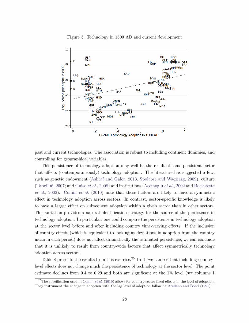
Figure 3: Technology in 1500 AD and current development

past and current technologies. The association is robust to including continent dummies, and

controlling for geographical variables.

This persistence of technology adoption may well be the result of some persistent factor

that affects (contemporaneously) technology adoption. The literature has suggested a few,

such as genetic endowment (Ashraf and Galor, 2013, Spolaore and Wacziarg, 2009), culture

(Tabellini, 2007; and Guiso et al., 2008) and institutions (Acemoglu et al., 2002 and Bockstette

et al., 2002). Comin et al. (2010) note that these factors are likely to have a symmetric

effect in technology adoption across sectors. In contrast, sector-specific knowledge is likely

to have a larger effect on subsequent adoption within a given sector than in other sectors.

This variation provides a natural identification strategy for the source of the persistence in

technology adoption. In particular, one could compare the persistence in technology adoption

at the sector level before and after including country time-varying effects. If the inclusion

of country effects (which is equivalent to looking at deviations in adoption from the country

mean in each period) does not affect dramatically the estimated persistence, we can conclude

that it is unlikely to result from country-wide factors that affect symmetrically technology

adoption across sectors.

Table 8 presents the results from this exercise.25 In it, we can see that including country-

level effects does not change much the persistence of technology at the sector level. The point

estimate declines from 0.4 to 0.29 and both are significant at the 1% level (see columns 1

25The specification used in Comin et al. (2010) allows for country-sector fixed effects in the level of adoption.They instrument the change in adoption with the lag level of adoption following Arellano and Bond (1991).

28

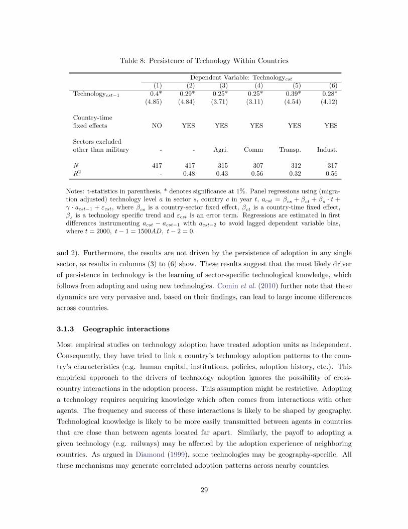
Table 8: Persistence of Technology Within Countries

Dependent Variable: Technologycst

(1) (2) (3) (4) (5) (6)Technologycst−1 0.4* 0.29* 0.25* 0.25* 0.39* 0.28*

(4.85) (4.84) (3.71) (3.11) (4.54) (4.12)

Country-timefixed effects NO YES YES YES YES YES

Sectors excludedother than military - - Agri. Comm Transp. Indust.

N 417 417 315 307 312 317R2 - 0.48 0.43 0.56 0.32 0.56

Notes: t-statistics in parenthesis, * denotes significance at 1%. Panel regressions using (migra-tion adjusted) technology level a in sector s, country c in year t, acst = βcs + βct + βs · t +γ · acst−1 + εcst, where βcs is a country-sector fixed effect, βct is a country-time fixed effect,βs is a technology specific trend and εcst is an error term. Regressions are estimated in firstdifferences instrumenting acst − acst−1 with acst−2 to avoid lagged dependent variable bias,where t = 2000, t− 1 = 1500AD, t− 2 = 0.

and 2). Furthermore, the results are not driven by the persistence of adoption in any single

sector, as results in columns (3) to (6) show. These results suggest that the most likely driver

of persistence in technology is the learning of sector-specific technological knowledge, which

follows from adopting and using new technologies. Comin et al. (2010) further note that these

dynamics are very pervasive and, based on their findings, can lead to large income differences

across countries.

3.1.3 Geographic interactions

Most empirical studies on technology adoption have treated adoption units as independent.

Consequently, they have tried to link a country’s technology adoption patterns to the coun-

try’s characteristics (e.g. human capital, institutions, policies, adoption history, etc.). This

empirical approach to the drivers of technology adoption ignores the possibility of cross-

country interactions in the adoption process. This assumption might be restrictive. Adopting

a technology requires acquiring knowledge which often comes from interactions with other

agents. The frequency and success of these interactions is likely to be shaped by geography.

Technological knowledge is likely to be more easily transmitted between agents in countries

that are close than between agents located far apart. Similarly, the payoff to adopting a

given technology (e.g. railways) may be affected by the adoption experience of neighboring

countries. As argued in Diamond (1999), some technologies may be geography-specific. All

these mechanisms may generate correlated adoption patterns across nearby countries.

29

In the development literature, several studies have explored how the neighbors’ adoption

decision affect and agent’s own decision. Foster and Rosenzweig (1995) study the adoption

of high-yield varieties in Indian villages. They find that the profitability of this technology

was increasing and concave in the neighbors’ experience with the seeds. Bandiera and Rasul

(2006) study the diffusion of sunflowers in Mozambique finding positive effects of neighbors

adoption decisions on a farmer’s adoption when few neighbors have adopted, but negative

when a significant number of neighbors has. Conley and Udry (2010) study the fertilizer

behavior of pineapple farmers in Ghana. They observe that a farmer will tend to imitate

neighbors’ fertilizer behavior when the neighbor has been successful in the past. This effect

is stronger when the farmer has little experience of his own.26

Despite its importance, it is still difficult to ascertain the generality of the findings from ex-

isting micro studies. In particular, are informational frictions and social interactions relevant

for other technologies (e.g. in other sectors, more complex, or more capital intensive)? And

how relevant are informational frictions and interactions once the focus moves from explaining

adoption differences among individuals to cross-country differences?

To explore the empirical importance of these mechanisms, Comin et al. (2013) (CDR,

henceforth) measure how far a country is from the high-density points in the distribution of

technology adoption in the other countries. They denote this measure of the spatial distance

from other country’s technology SDT. A negative correlation between SDT and adoption,

after controlling for country and time fixed effects, implies that countries that are further

away from those where the technology diffuses faster tend to experience a slower adoption of

the technology.

Using data on twenty technologies from CHAT, they find a strong and significant negative

partial correlation between SDT and a country’s adoption. The estimates imply that spatial

interactions that facilitate technology adoption decline by 73% every 1000 Kms. The estimates

are robust to controlling for income, human capital, trade openness, institutions and for the

spatial distance from other countries per-capita income (SDI), constructed in a way parallel

to SDT.

To further explore the nature of the interactions that is causing the effect, CDR also

explore whether the effect of other countries’ technology evolves as the technology diffuses.

Note that, interactions mediated by the flow of people or of goods and services would tend to

persist over time. In contrast, interactions driven by the diffusion of knowledge should tend

to vanish over time as knowledge is easier to replicate within one location. Consistent with

this later hypothesis, CDR find that the effect of SDT on technology adoption diminishes as

the diffusion process unfolds.

A final question CDR take on is Jared Diamond’s hypothesis that technologies diffuse

26Similar neighbor effects have been observed in bed nets Dupas (2009). See Foster and Rosenzweig (2010)for a survey of the development literature.

30

along latitudes. To explore this, they decompose SDT between two components one based on

distances along latitudes and another based on distances along longitudes. Consistent with

Diamond (1999), they find that latitude component of SDT has a stronger association with

technology adoption than longitude component of SDT, although both have a significant effect.

This finding is remarkable since their sample does not include any technology where climatic

reasons might suggest that distance across latitudes is a larger impediment for diffusion than

distance across longitudes.

One last form of geographic interaction considered in the literature is migration flows.

International migration may have brought significant technological knowledge from areas with

more advanced technologies to others where advanced technologies were rare. If that is the

case, one would expect that adjusting knowledge flows by the movement of people should

provide a more accurate account of the cross-country dynamics of productivity. With this

idea in mind, Putterman and Weil (2010) explore whether the history of people matters

more than history of places by measuring, for each country, the origin of the ancestors of

today’s population, going back to 1500AD. Putterman and Weil show that, after adjusting for

historical migration flows, variables such as the antiquity of states and years of experience with

agriculture have a greater explanatory power of current development. Comin et al. (2010)

extend Putterman and Weil’s analysis by applying the Putterman-Weil migration matrix

to the historical technology adoption in 1500AD. This yields a measure of the historical

adoption level in 1500AD of the ancestors to the people that live today in each country.

With this migration-adjusted measures of technology, they re-examine their exploration of

the persistence of technology adoption.

Figure 4 shows the simple scatter plot between migration-adjusted technological heritage

from 1500 A.D. and per capita income today. Comparing Figure 4 with Figure 3, it is clear

that long-run technological persistence is stronger overall if we base technology on peoples

rather than places (the R-squared increases from .18 to .50). A movement from 0 to 1 is

associated with an increase in per capita income today by a factor of 26.1! Similarly, this

regression implies that 78 percent of the log difference in income today between sub-Saharan

Africa and Western Europe is associated with the technology differences in 1500 A.D. Based

on this evidence, it is clear that the propagation of technological knowledge through migration

flows is an important source of cross-country differences in technology adoption.

3.2 Institutions and policies

In the same way that insufficient technological knowledge constrains the agents’ ability to

use a new technology in a productive way, inadequate political institutions may reduce the

agents’ incentive to incur in the costs of using a new technology. There is no lack of theoreti-

cal arguments and anecdotal evidence that point to specific mechanisms by which inadequate

31

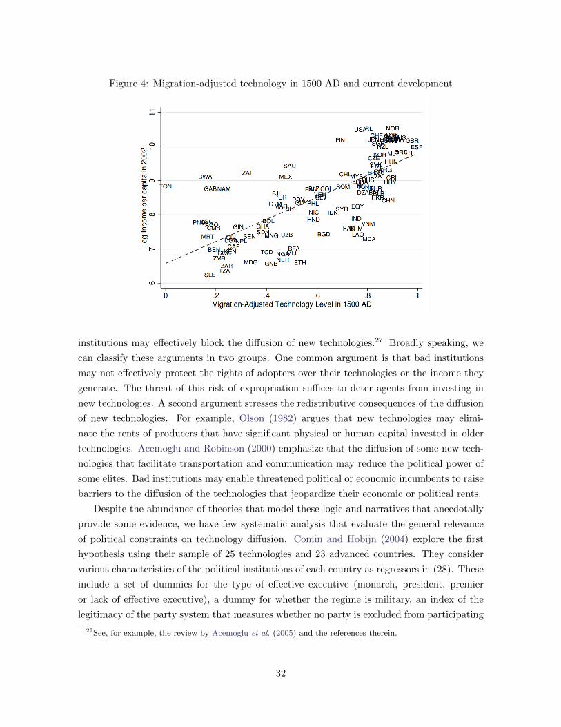
Figure 4: Migration-adjusted technology in 1500 AD and current development

institutions may effectively block the diffusion of new technologies.27 Broadly speaking, we

can classify these arguments in two groups. One common argument is that bad institutions

may not effectively protect the rights of adopters over their technologies or the income they

generate. The threat of this risk of expropriation suffices to deter agents from investing in

new technologies. A second argument stresses the redistributive consequences of the diffusion

of new technologies. For example, Olson (1982) argues that new technologies may elimi-

nate the rents of producers that have significant physical or human capital invested in older

technologies. Acemoglu and Robinson (2000) emphasize that the diffusion of some new tech-

nologies that facilitate transportation and communication may reduce the political power of

some elites. Bad institutions may enable threatened political or economic incumbents to raise

barriers to the diffusion of the technologies that jeopardize their economic or political rents.

Despite the abundance of theories that model these logic and narratives that anecdotally

provide some evidence, we have few systematic analysis that evaluate the general relevance

of political constraints on technology diffusion. Comin and Hobijn (2004) explore the first

hypothesis using their sample of 25 technologies and 23 advanced countries. They consider

various characteristics of the political institutions of each country as regressors in (28). These

include a set of dummies for the type of effective executive (monarch, president, premier

or lack of effective executive), a dummy for whether the regime is military, an index of the

legitimacy of the party system that measures whether no party is excluded from participating

27See, for example, the review by Acemoglu et al. (2005) and the references therein.

32

in the political process. Table 7 reproduces their findings. There are two main observations.

First, both not having an effective executive and having a military regime are associated with a

lower level of technology in the country. This is consistent with the notion that property right

protection is a necessary condition for adopting technologies. Second, an effective legislature

is associated with a less intense adoption of technologies. This finding may be surprising, but

we try to rationalize it below.

The role of redistributive politics on technology diffusion has also been explored recently.

Comin and Hobijn (2009b) bring to the data Olson (1982) theory and explore the significance

of barriers erected by incumbent producers on the speed of diffusion of new technologies. Their

identification strategy consists in two parts. First, certain institutional attributes affect the

political cost faced by the legislature when raising barriers to the diffusion of a new technology.

In particular, the cost lobbies must incur to induce legislators to raise diffusion barriers are

higher when legislators are not independent, the judicial system is effective, and the regime

is democratic and non-military.28

Second, the benefits old technology producers enjoy from raising barriers against the

diffusion of a new technology depend on certain attributes of the new and old technologies.

There are some new technologies that are so superior to the old technology that, even with

political barriers, consumers prefer the new technology to the old one. In these cases, old

technology producers find no benefit in lobbying for barriers. Thus, the new technology

will diffuse quickly regardless of the costs of lobbying. Other new technologies do, however,

have close predecessor technologies because the productivity differential between old and new

technologies is relatively small. In these cases, old technology producers may benefit from

barriers to the new technology because in the presence of barriers consumers may prefer to use

the old technology. The speed of diffusion of these new technologies depends, therefore, on the

cost of erecting barriers. When it is costly to raise political barriers, lobbying is unsuccessful,

barriers are not raised, and new technologies diffuse quickly. Conversely, when the cost of

raising barriers is low, the legislative authority accepts the old technology’s lobbying bribes

and raises barriers that slow down the diffusion of the new technology.

It follows from these two premises that, the effect of lobbies on technology diffusion can

be identified by the differential effect of institutions. If lobbies matter, institutions that

affect the political cost of erecting barriers should have a differential effect on the diffusion of

technologies with close predecessors relative to those without close predecessors.

Comin and Hobijn use a sample of 20 technologies, 23 countries over the last 200 years

from HCCTAD. Their main finding is that variables that affect the cost of lobbying such as

how democratic is a country, the judicial effectiveness and whether the regime is military have

a differential effect on the diffusion of technologies with a close predecessor of the expected

28See, Myerson (1993), Ferejohn (1986), Persson et al. (2000), Kunicova and Rose-Ackerman (2005), Perssonet al. (2003) and Besley and Case (1995).

33

sign (higher cost is associated with higher differential adoption). Similarly, Comin and Hobijn

(2009b) find that a more independent legislative power is associated with a negative differential

diffusion of the technologies with a close predecessor. They rationalize as evidence that, other

things equal, a more independent legislature faces less constraints to pass regulations that

favor powerful lobbies, which tend to be those of the incumbent technologies. It is important

to stress that these results are robust to including country and year dummies as well as

country-dummies that are specific to incumbent and new technology groupings.

Though the evidence presented in Comin and Hobijn (2009b) is supportive of the role

of distributive politics on technology diffusion, it is important to be aware of two important

limitations of this study. First, it evaluates only one particular theory of redistributive pol-

itics and technology diffusion Olson, 1982. Second, the sample used covers only advanced

economies. Hence, more studies are necessary to made an accurate assessment of the global

significance of political institutions on technology adoption patterns.

Trade Openness One of the reasons why institutions may matter is because they affect the

policies implemented by governments. Among those, trade policies have probably received

most attention. Sachs and Warner (1995), Frankel and Romer (1999) and Feyrer (2009a,b)

showed that trade has a significant impact on income growth. A natural question is whether

the channel by which trade affects growth is technology adoption. This question is still largely

unexplored. All the existing evidence we are aware off basically consists in including measures

of trade openness in specification (28).29 Comin and Hobijn (2004) find that countries whose

trade makes up a larger part of its GDP are the front runners in technology adoption. The

coefficient on openness is significant for the bulk of our specifications and its magnitude implies

that countries that are 12–15% more open than others will be 1% ahead in the adoption of

technologies.

Related to this, Coe and Helpman (1995) find a strong effect of the technological ad-

vancement of the trading partner on TFP. Again, it is natural to inquire whether this effect

operates through the adoption of new technologies. To explore this hypothesis, Comin and Ho-

bijn (2004) include as regressors the trade-weighted averages of GDP and the trade-weighted

level of technology adoption for the trading partners. Somewhat surprisingly, they obtain a

negative coefficient which they interpret as evidence that the effect of trade on TFP may be

affecting factors other than a more intensive adoption of technology. Again, this seems an

area where there is room for more research in the future.

29Lucas et al. (2011) and Perla et al. (2012) provide structural models of trade and growth that account forthe diffusion process. They rely on calibrations to assess the link between trade and growth.

34

3.3 Demand

The level of demand is an important determinant of the return to adopting a technology. A

higher demand allows adopters to cover the sunk costs of adoption among more buyers of the

goods and services produced with the technology. Therefore, increasing the profitability of the

investment. Even when the costs of adoption are negligible, we should expect larger demand

for the goods and services that embody a technology in places and times where aggregate

demand is higher. This is clear from equation (22).

The notion that demand is an important driver of technology has been recognized at least

since Schmookler (1966). Schmookler argued that demand should play a key role both in the

amount of innovation activity as well as in the sectors where it was concentrated. He brought

this hypothesis to the data by exploring how patenting activity in capital intensive sectors

correlated with lagged investment (his measure of demand pull). Both in cross-sections of

sectors and in the time series within sectors, Schmookler (1966) found a strong co-movement

between lagged investment and patenting activity.30 Subsequent research has explored the

cyclicality of R&D activities (Griliches, 1990, Fatas, 2000, Comin and Gertler, 2006). The

robust finding is that R&D expenditures positively co-move with output at business cycle

frequencies and that the co-movement increases when we consider lower frequencies.31 Most

of this evidence is at the aggregate level. The exception is Barlevy (2007), who found a

positive co-movement between firm-level growth in real R&D expenditures and 4-digit sector

level growth in aggregate demand.

Nevertheless, R&D and technology adoption are distinct activities that are undertaken by

different companies and that also differ in their geography. Is there evidence of the importance

of demand pull forces for the adoption of new technologies?

In Table 7, Comin and Hobijn (2004) introduce the log of income per capita as a control

(see equation 28). They find that the elasticity of technology with respect to income is around

1 (and significant at the 1% level). Of course, the concern that per capita income captures

variables other than demand is legitimate. This concern, however should be mitigated to some

extent by the fact that the estimate of the income elasticity does not decline after controlling

for potential omitted variables such as institutions, openness, human capital and adoption of

predecessor and complementary technologies.

Comin (2009) follows a different approach to estimating the elasticity of technology with

respect to income. Following the traditional diffusion literature, he poses a S-shaped diffusion

process modified to allow for the speed of diffusion to depend on deviations from trend of

GDP. In particular, consider the (log) ratio of adopters (mjt) to non-adopters (M −mjt) for

30See Scherer (1981) for a confirmation of these findings in a larger number of sectors and other indicatorsof demand pull.

31Specifically, cycles with periods between 8 and 50 years.

35

a generic technology j

rjt ≡ ln(mjt/(M −mjt)).

Note that the first difference of rjt is the speed of diffusion of the technology. If the share

of adopters (mjt/M) follows a logistic curve, then the speed of diffusion (4rjt) is constant.

Comin explores the constancy of the speed of diffusion in a sample of 22 manufacturing

processes in the UK.32 He finds that the speed of diffusion is far from constant and it tends

to decline as the technology diffuses. To capture this pattern and to explore the cyclicality of

the speed of technology diffusion, Comin (2009) poses the following specification

4rjt+1 = βj + α1tj + α2t2j + γy2200t + εjt, (29)

where tj is the number of years since the invention of technology j, and y2200t is GDP detrended

so that we keep fluctuations with periods between 2 and 200 quarters.

Comin (2009) obtains an estimate of the elasticity of the speed of diffusion with respect

to detrended GDP of 5.12 with a 95% confidence interval of (1.9, 8.34). Figure 5 plots the

implications of equation (29) for the diffusion of numerical control turning machines. The

black solid line represents the actual evolution of the share of adopters; the line with triangles

plots the diffusion path predicted by equation (29); the line with starts plots the evolution of

cumulative detrended output; and the line with squares plots the diffusion path predicted by

equation (29) when the effect of the cycle on diffusion is ignored.

Ignoring the business cycle component in equation (29) has important consequences. Eight

years after the introduction of numerical control turning machines in the UK only seven

percent of potential adopters had adopted the technology. The model without the cycle

component predicts that over 30 percent of potential adopters should be using the technology.

One explanation for the slow diffusion of numerical control turning machines in the UK is

that at that point it had been for eight consecutive years below trend. As a result producers

faced a low demand and had few incentives to invest in the new technology. Once this effect

is taken into account, equation (29) predicts that after eight years the diffusion of numerical

control turning machines in the UK should have been 13 percent, much closer to the actual

seven percent.

This evidence raises the question of why are the estimates for the income elasticity of

technology so different in Comin (2009) and Comin and Hobijn (2004). Is the difference due

to differences in the measurement of technology, or to differences in the income frequencies

32The data comes from Davies (1979) and spans from WWII to the late 1970s. The technologies includespecial presses, foils, wet suction boxes, gibberellic acid, automatic size boxes, accelerated drying hoods,electrical hygrometers, basic oxygen process, vacuum degassing, vacuum melting, continuous casting, tunnelkilns, process control by computer, tufted carpets, computer typesetting, photo-electrically controlled cutting,shuttleless looms, numerical control printing presses, numerical control turning machines and numerical controlturbines.

36

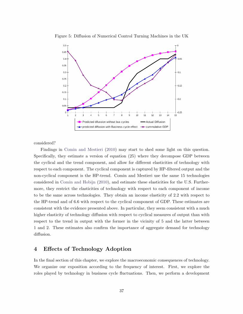
Figure 5: Diffusion of Numerical Control Turning Machines in the UK

considered?

Findings in Comin and Mestieri (2010) may start to shed some light on this question.

Specifically, they estimate a version of equation (25) where they decompose GDP between

the cyclical and the trend component, and allow for different elasticities of technology with

respect to each component. The cyclical component is captured by HP-filtered output and the

non-cyclical component is the HP-trend. Comin and Mestieri use the same 15 technologies

considered in Comin and Hobijn (2010), and estimate these elasticities for the U.S. Further-

more, they restrict the elasticities of technology with respect to each component of income

to be the same across technologies. They obtain an income elasticity of 2.2 with respect to

the HP-trend and of 6.6 with respect to the cyclical component of GDP. These estimates are

consistent with the evidence presented above. In particular, they seem consistent with a much

higher elasticity of technology diffusion with respect to cyclical measures of output than with

respect to the trend in output with the former in the vicinity of 5 and the latter between

1 and 2. These estimates also confirm the importance of aggregate demand for technology

diffusion.

4 Effects of Technology Adoption

In the final section of this chapter, we explore the macroeconomic consequences of technology.

We organize our exposition according to the frequency of interest. First, we explore the

roles played by technology in business cycle fluctuations. Then, we perform a development

37

accounting exercise. We quantify the contribution of cross-country differences in technology

diffusion to cross-country differences in income. Finally, we explore how changes in technology

adoption patterns over time help us explain cross-country growth differences over protracted

periods of time.

4.1 Business Cycles Fluctuations

The role conferred to technology in business cycle analysis has traditionally been reduced to

an exogenous disturbance. This is a natural consequence of using the neoclassical growth

model as the workhorse framework for business cycle analysis. Real business cycle models

(e.g., Kydland and Prescott, 1982) intend to synthesize growth and business cycle fluctuations

by introducing stochastic disturbances to the exogenous technology process. The propagation

of the shocks is then governed by the dynamics of capital accumulation in the neoclassical

model. In early versions of RBC models, total factor productivity (TFP) is interpreted as

a measure of the technology in the economy. Growth in TFP drives growth in the long

term. TFP has two components. A deterministic trend and exogenous, stochastic deviations

from the trend that drive short-term fluctuations in the economy. Subsequent approaches to

business cycle analysis have minimized the role of technology shocks as a source of business

cycle fluctuations (Galı, 1999) and have re-interpreted the observed short-term fluctuations

in TFP as reflecting cyclical variation in the intensity of use of the factors of production or

in the degree of competition (Burnside et al., 1995 and Basu and Fernald, 1997).

Next, we review two new lines of work on the role of technology on business cycle fluc-

tuations. The first re-examines the classical question of the importance of technology shocks

for business fluctuations by using more direct measures of technology in the identification of

technology shocks. The second line of work proposes technology as a propagation mechanism

based on the evidence discussed above on the cyclicality of R&D expenditures and the speed

of diffusion of technology.

4.1.1 Shocks

The identification of technology shocks has been challenging in macroeconomics. Traditional

approaches involve using indirect inference techniques based either or modified Solow residuals

(e.g., Basu, 1996) or on restrictions on the responses from vector-autoregression (VAR) models

(e.g., Galı, 1999). Alexopoulos (2011) revises the classical question of what is the short term

effect of a technology shock using her technology books measure to identify technology shocks.

To explore this issue, she detrends the measures of the number of technology books edited

using a band-pass filter that permits her to consider two types of frequencies: the business

cycle (periods between 2 and 8 years) the medium term cycle (periods between 2 and 30

38

years).33

Alexopoulos shows that both at high and medium term frequencies, her technology mea-

sures lead GDP fluctuations. The highest correlations are between the number of books

published on computer software and hardware and GDP at t+ 1 which she finds to be 0.47.

Technology books also lead investment and TFP by one or two years, specially when con-

sidering medium term cycles.34 Interestingly, the number of technology books edited have

a sizable volatility both over the business cycle and the medium term cycle. As a way of

comparison. the standard deviation of the high frequency measure of technology books edited

with lowest volatility–Alexopoulos has 5 different measures– has a standard deviation of 3.5%

vs. 1.4% for GDP. Estimating a bivariate system where log GDP is ordered first and the

technology measure second, she finds that, at a 3 years horizon, technology accounts for at

least 9% of business fluctuations in log GDP and, at a 9 years horizon, this figure raises to

37%. These figures suggests that fluctuations in the technology available to firms (as proxied

by the number of technology books edited) may be a significant source of business cycles

fluctuations.

4.1.2 Propagation mechanisms

As showed by Cogley and Nason (1995), capital accumulation dynamics are a weak propaga-

tion mechanism. The persistence of RBC models is basically the persistence of their shocks.

As a result, these models do not explain the persistence of macro variables, they just assume

it (in the form of persistent shocks). This approach is clearly unsatisfactory. On the one

hand, macro shocks typically are not as persistent as macro series. On the other, it is of criti-

cal importance both for descriptive and prescriptive reasons to understand what mechanisms

propagate short term shocks and generate effects that last for several quarters and years.

Comin and Gertler (2006) explore this question by deviating from the standard macro

framework. In particular, based on the evidence that R&D and adoption investments are pro-

cyclical, they challenge the view that technology is exogenous. They do that by building a

business cycle model where, as in endogenous growth models (e.g., Romer, 1990), technology

is the result from purposeful investments by agents/firms in developing and adopting new

technologies. The investments in upgrading technology (by innovation or adoption) affect the

stock of technologies available for production. In this way, technology emerges naturally as a

new state variable that may significantly affect the dynamic response of the model to business

cycle shocks.

33Note that she uses an upper bound that is slightly lower than the one used in Comin and Gertler (2006).34With respect to hours, Alexopoulos finds that there is no significant contemporaneous effect of technology

on hours work at the high frequency but she finds strong positive effects of current technology on hours at t+1and at t + 2. Over the medium term, she finds a negative and sizable contemporaneous association betweenhours and technology and a milder effect after one and two years.

39

Next, we sketch a simplified version of the framework developed in Comin and Hobijn

(2007) and review its implications.

A business cycle framework with endogenous technology Our description focuses

mostly in the production side of the economy. This version of the framework is a one sector

model with development and adoption of intermediate goods which affect the efficiency of

production in the economy.

Final output.– Final output is produced competitively according to

Yt =((UtKt)

α L1−αt

)γM1−γt , (30)

where Ut denotes the intensity of utilization of capital, Kt, Lt denotes hours worked and Mt

denotes the materials used in production. Utilization comes at the cost of a faster depreciation

of capital. Materials are produced competitively combining differentiated intermediate goods

according to

Mt =

(∫ At

0x

1/θit

)θ,

where θ > 1 will also be the markup charged by the producer of intermediate good i. It takes

one unit of final output to produce one unit of any intermediate good. At denotes the number

of intermediate goods available for production at time t. Note that if producers use the same

number of units of all intermediate goods available for production (e.g., xt), then (30) can be

expressed as

Yt = A(1−γ)(θ−1)t

((UtKt)

α L1−αt

)γ(Atxt)

1−γ . (31)

The last term in (31) is the amount of output used to produce intermediate goods and

the first term is the technological component of TFP.

Adoption.– Intermediate goods are first invented and then are adopted for production. We

first characterize the adoption process conditional on the available set of technologies, and

then describe the research and development process that leads to new technologies.

Let Zt denote the stock of invented technologies. The stock of not-yet-adopted technologies

is Zt−At. Each period, a fraction of the available new technologies become usable. Whether

a technology becomes usable is a random draw with success probably λt. Once a technology

is usable, all firms are able to employ it immediately. Note that under this setup there is slow

diffusion of new technologies on average (as on average there is a lag between their invention

and adoption dates). Furthermore, aggregation is simple as once a technology is in use, all

firms have it.

Formally, the number of adopted technologies, At is given by

At = λt[Zt−1 −At−1] + φAt−1 (32)

40

with 0 < φ < 1 representing the probability that the technology has not become obsolete in

one period, and 0 < λt < 1. We assume that λt is given by the following function

λt = λ(Γtht)

with λ′ > 0, λ′′ < 0, where Γt is the scaling factor that guarantees the existence of a balanced-

growth path and exogenous to the adopter and ht are the resources devoted to adopting a

technology in time t.35

If φ is close to 1, it follows from (32) that transitory changes in λt will have transitory

changes in the growth rate of At, but close to permanent changes in the level of At. This prop-

erty is key to making endogenous technology a powerful propagation mechanism. However, it

is not sufficient. In addition, it is necessary that λt is pro-cyclical. To explore the cyclicality

of λt, we next endogenize it.

The value to the adopter of successfully bringing a new technology into use, vt, is given by

the present value of profits from operating the technology. Profits each period πt arise from

the fact that the producer of the new good is a monopolistic competitor. Accordingly, given

that Rt+1 is the one period discount rate between t+ 1 and t, we can express, vt, as

vt = πt + φEt

[vt+1

Rt+1

]. (33)

If an adopter is unsuccessful in the current period, he may try again in the subsequent period

to make the technology usable. Let wt be the value of acquiring an innovation that has not

yet been adopted. wt is given by

wt = maxht−ht + φEt

[[λ (Γtht) vt+1 + (1− λ (Γtht))wt+1]

Rt+1

]. (34)

At the margin, adopters determine how much to spend in adopting a technology by equal-

izing the marginal cost and the expected marginal benefit from adoption:

1 = Et[R−1t+1φΓtλ

′ (Γtht) (vt+1 − wt+1)]. (35)

The expected marginal benefit has three terms. The first captures the discounting of the

potential benefits from adoption (i.e., R−1t+1φ); the second captures the marginal increase in

the probability of succeeding in adopting when firms invest one extra unit of output (i.e.,

Γtλ′ (Γtht)); the third captures the capital gain that occurs when an intermediate good be-

comes adopted (i.e., vt+1 − wt+1). When the economy is booming, the expected capital gain

increases because of the higher demand of adopted intermediate goods. Firms respond to

35Comin and Gertler (2006) model Γt as inversely proportional to the (wholesale) value of capital. It isimportant that Γt is smooth.

41

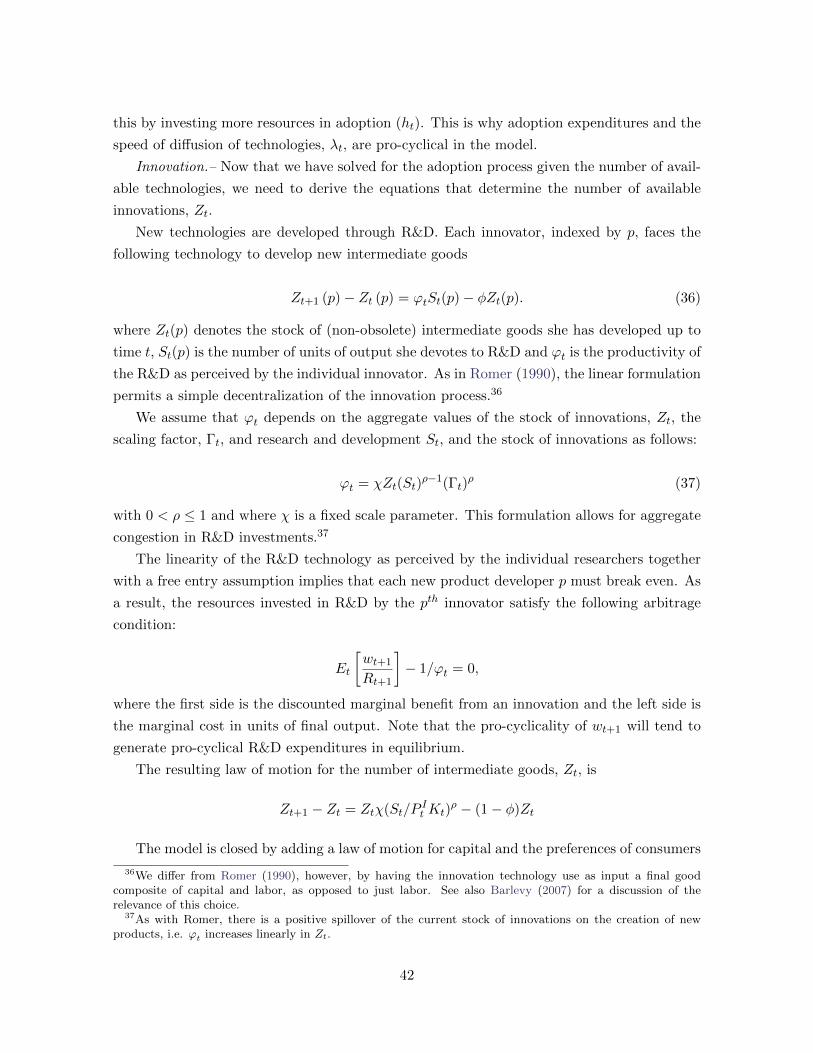
this by investing more resources in adoption (ht). This is why adoption expenditures and the

speed of diffusion of technologies, λt, are pro-cyclical in the model.

Innovation.– Now that we have solved for the adoption process given the number of avail-

able technologies, we need to derive the equations that determine the number of available

innovations, Zt.

New technologies are developed through R&D. Each innovator, indexed by p, faces the

following technology to develop new intermediate goods

Zt+1 (p)− Zt (p) = ϕtSt(p)− φZt(p). (36)

where Zt(p) denotes the stock of (non-obsolete) intermediate goods she has developed up to

time t, St(p) is the number of units of output she devotes to R&D and ϕt is the productivity of

the R&D as perceived by the individual innovator. As in Romer (1990), the linear formulation

permits a simple decentralization of the innovation process.36

We assume that ϕt depends on the aggregate values of the stock of innovations, Zt, the

scaling factor, Γt, and research and development St, and the stock of innovations as follows:

ϕt = χZt(St)ρ−1(Γt)

ρ (37)

with 0 < ρ ≤ 1 and where χ is a fixed scale parameter. This formulation allows for aggregate

congestion in R&D investments.37

The linearity of the R&D technology as perceived by the individual researchers together

with a free entry assumption implies that each new product developer p must break even. As

a result, the resources invested in R&D by the pth innovator satisfy the following arbitrage

condition:

Et

[wt+1

Rt+1

]− 1/ϕt = 0,

where the first side is the discounted marginal benefit from an innovation and the left side is

the marginal cost in units of final output. Note that the pro-cyclicality of wt+1 will tend to

generate pro-cyclical R&D expenditures in equilibrium.

The resulting law of motion for the number of intermediate goods, Zt, is

Zt+1 − Zt = Ztχ(St/PIt Kt)

ρ − (1− φ)Zt

The model is closed by adding a law of motion for capital and the preferences of consumers

36We differ from Romer (1990), however, by having the innovation technology use as input a final goodcomposite of capital and labor, as opposed to just labor. See also Barlevy (2007) for a discussion of therelevance of this choice.

37As with Romer, there is a positive spillover of the current stock of innovations on the creation of newproducts, i.e. ϕt increases linearly in Zt.

42

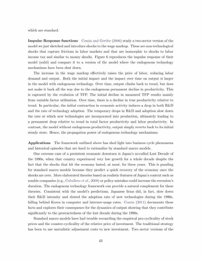
which are standard.

Impulse Response functions Comin and Gertler (2006) study a two-sector version of the

model we just sketched and introduce shocks to the wage markup. These are non-technological

shocks that capture frictions in labor markets and that are isomorphic to shocks to labor

income tax and similar to money shocks. Figure 6 reproduces the impulse response of their

model (solid) and compare it to a version of the model where the endogenous technology

mechanisms have been shut down.

The increase in the wage markup effectively raises the price of labor, reducing labor

demand and output. Both the initial impact and the impact over time on output is larger

in the model with endogenous technology. Over time, output climbs back to trend, but does

not make it back all the way due to the endogenous permanent decline in productivity. This

is captured by the evolution of TFP. The initial decline in measured TFP results mainly

from variable factor utilization. Over time, there is a decline in true productivity relative to

trend. In particular, the initial contraction in economic activity induces a drop in both R&D

and the rate of technology adoption. The temporary drops in R&D and adoption slow down

the rate at which new technologies are incorporated into production, ultimately leading to

a permanent drop relative to trend in total factor productivity and labor productivity. In

contrast, the model without endogenous productivity, output simply reverts back to its initial

steady state. Hence, the propagation power of endogenous technology mechanisms.

Applications The framework outlined above has shed light into business cycle phenomena

and historical episodes that are hard to rationalize by standard macro models.

One extreme case of a persistent economic downturn is Japan’s so-called Lost Decade of

the 1990s, when that country experienced very low growth for a whole decade despite the

fact that the shocks that hit the economy lasted, at most, for three years. This is puzzling

for standard macro models because they predict a quick recovery of the economy once the

shocks are over. More elaborated theories based on realistic features of Japan’s context such as

zombie companies (e.g., Caballero et al., 2008) or policy mistakes could increase the recession’s

duration. The endogenous technology framework can provide a natural complement for these

theories. Consistent with the model’s predictions, Japanese firms did, in fact, slow down

their R&D intensity and slowed the adoption rate of new technologies during the 1990s,

falling behind Korea in computer and internet-usage rates. Comin (2011) documents these

facts and explores their consequence for the dynamics of output showing that they contribute

significantly to the protractedness of the lost decade during the 1990s.

Standard macro models have had trouble reconciling the empirical pro-cyclicality of stock

prices and the counter-cyclicality of the relative price of investment. The traditional strategy

has been to use unrealistic adjustment costs to new investment. Two sector versions of the

43

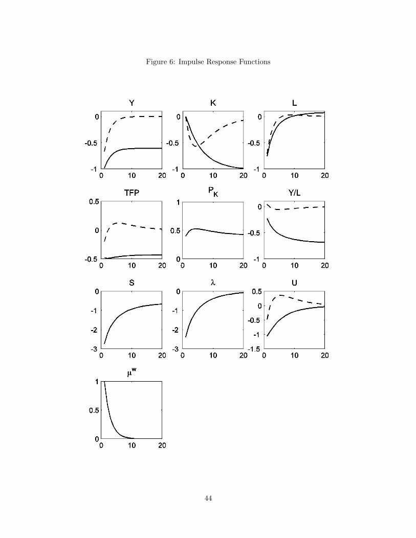
Figure 6: Impulse Response Functions

44

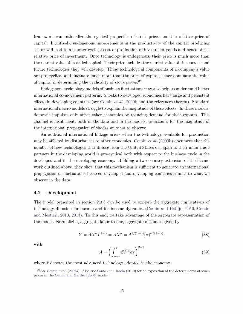
framework can rationalize the cyclical properties of stock prices and the relative price of

capital. Intuitively, endogenous improvements in the productivity of the capital producing

sector will lead to a counter-cyclical cost of production of investment goods and hence of the

relative price of investment. Once technology is endogenous, their price is much more than

the market value of installed capital. Their price includes the market value of the current and

future technologies they will develop. These technological components of a company’s value

are pro-cyclical and fluctuate much more than the price of capital, hence dominate the value

of capital in determining the cyclicality of stock prices.38

Endogenous technology models of business fluctuations may also help us understand better

international co-movement patterns. Shocks to developed economies have large and persistent

effects in developing countries (see Comin et al., 2009b and the references therein). Standard

international macro models struggle to explain the magnitude of these effects. In these models,

domestic impulses only affect other economies by reducing demand for their exports. This

channel is insufficient, both in the data and in the models, to account for the magnitude of

the international propagation of shocks we seem to observe.

An additional international linkage arises when the technology available for production

may be affected by disturbances to other economies. Comin et al. (2009b) document that the

number of new technologies that diffuse from the United States or Japan to their main trade

partners in the developing world is pro-cyclical both with respect to the business cycle in the

developed and in the developing economy. Building a two country extension of the frame-

work outlined above, they show that this mechanism is sufficient to generate an international

propagation of fluctuations between developed and developing countries similar to what we

observe in the data.

4.2 Development

The model presented in section 2.3.3 can be used to explore the aggregate implications of

technology diffusion for income and for income dynamics (Comin and Hobijn, 2010, Comin

and Mestieri, 2010, 2013). To this end, we take advantage of the aggregate representation of

the model. Normalizing aggregate labor to one, aggregate output is given by

Y = AXαL1−α = AXα = A1/(1−α)(α)α/(1−α), (38)

with

A =

(∫ τ

−∞Z

1θ−1τ dτ

)θ−1

(39)

where τ denotes the most advanced technology adopted in the economy.

38See Comin et al. (2009a). Also, see Santos and Iraola (2010) for an exposition of the determinants of stockprices in the Comin and Gertler (2006) model.

45

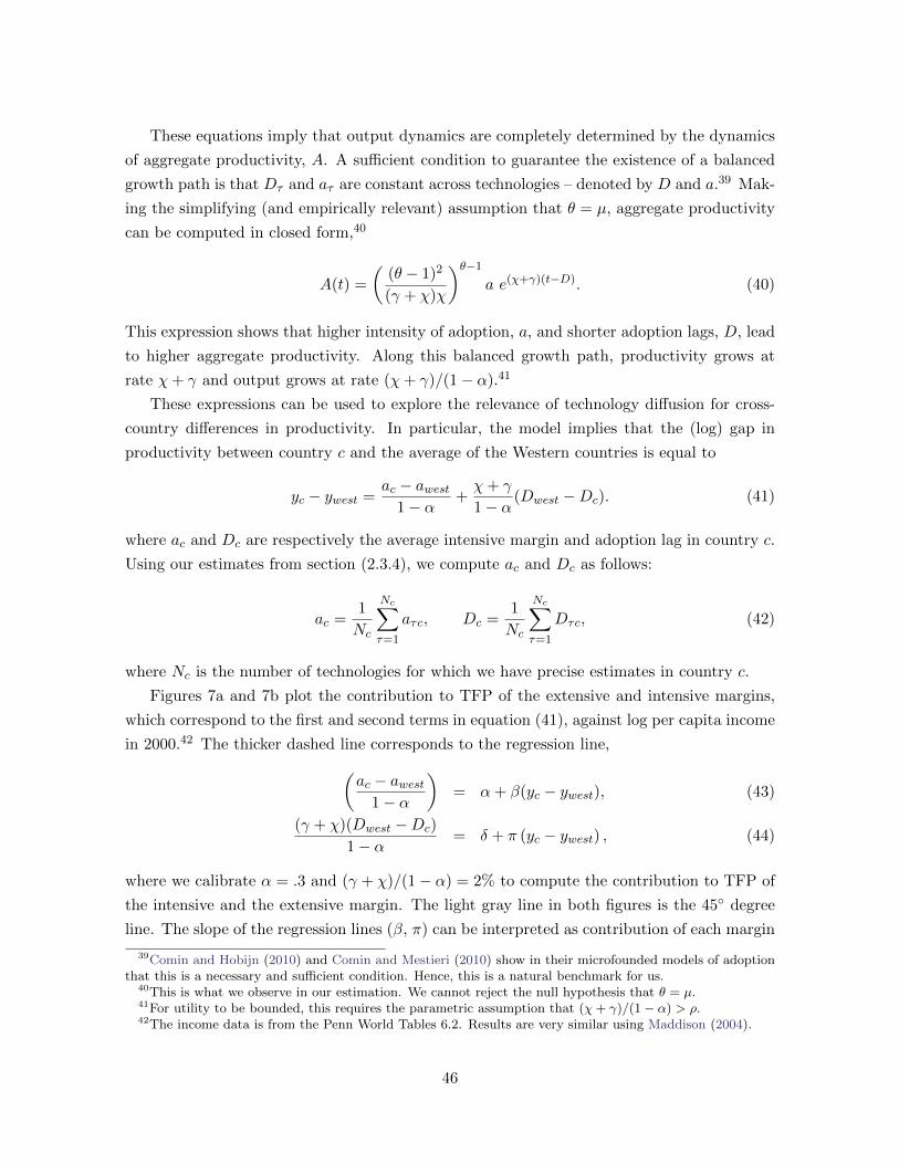
These equations imply that output dynamics are completely determined by the dynamics

of aggregate productivity, A. A sufficient condition to guarantee the existence of a balanced

growth path is that Dτ and aτ are constant across technologies – denoted by D and a.39 Mak-

ing the simplifying (and empirically relevant) assumption that θ = µ, aggregate productivity

can be computed in closed form,40

A(t) =

((θ − 1)2

(γ + χ)χ

)θ−1

a e(χ+γ)(t−D). (40)

This expression shows that higher intensity of adoption, a, and shorter adoption lags, D, lead

to higher aggregate productivity. Along this balanced growth path, productivity grows at

rate χ+ γ and output grows at rate (χ+ γ)/(1− α).41

These expressions can be used to explore the relevance of technology diffusion for cross-

country differences in productivity. In particular, the model implies that the (log) gap in

productivity between country c and the average of the Western countries is equal to

yc − ywest =ac − awest

1− α+χ+ γ

1− α(Dwest −Dc). (41)

where ac and Dc are respectively the average intensive margin and adoption lag in country c.

Using our estimates from section (2.3.4), we compute ac and Dc as follows:

ac =1

Nc

Nc∑τ=1

aτc, Dc =1

Nc

Nc∑τ=1

Dτc, (42)

where Nc is the number of technologies for which we have precise estimates in country c.

Figures 7a and 7b plot the contribution to TFP of the extensive and intensive margins,

which correspond to the first and second terms in equation (41), against log per capita income

in 2000.42 The thicker dashed line corresponds to the regression line,(ac − awest

1− α

)= α+ β(yc − ywest), (43)

(γ + χ)(Dwest −Dc)

1− α= δ + π (yc − ywest) , (44)

where we calibrate α = .3 and (γ + χ)/(1− α) = 2% to compute the contribution to TFP of

the intensive and the extensive margin. The light gray line in both figures is the 45◦ degree

line. The slope of the regression lines (β, π) can be interpreted as contribution of each margin

39Comin and Hobijn (2010) and Comin and Mestieri (2010) show in their microfounded models of adoptionthat this is a necessary and sufficient condition. Hence, this is a natural benchmark for us.

40This is what we observe in our estimation. We cannot reject the null hypothesis that θ = µ.41For utility to be bounded, this requires the parametric assumption that (χ+ γ)/(1− α) > ρ.42The income data is from the Penn World Tables 6.2. Results are very similar using Maddison (2004).

46

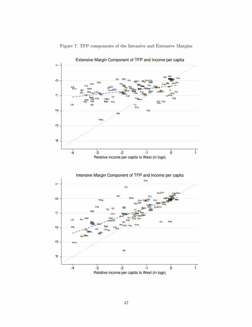
Figure 7: TFP components of the Intensive and Extensive Margins

47

in accounting for differences in income per capita in 2000. If equation (41) were to explain all

the income variation today, we would expect the coefficient of (each) regression to be 1 and

the data points to lie on the 45◦ degree line. We find that the slope for the extensive margin

regression displayed in Figure 7a is 20%, while for the intensive margin is almost 60%.43 If

these two margins were uncorrelated we could infer that these two margins alone account for

most of the variation (80%) of income per capita today. If we regress the extensive margin

on the intensive margin and use the unpredicted part as the orthogonal component of the

intensive margin not predicted by the extensive, we would find that the slope of figure 7b

goes down to 54%. Thus, most of the variation in income per capita today, over 70%, can

be accounted by cross-country differences in the two adoption margins. Among the two, the

intensive margin takes the lion’s share.

4.3 Growth

In this section we study how the evolution of the two margins of adoption affect the evolution

of aggregate productivity of the economy. We use the model from Section 2.3.2 to evaluate

quantitatively its ability to generate the observed cross-country income growth dynamics over

the last 200 years.

Specifically, we focus on three questions: (i) The significance of differences in early adop-

tion to account for cross-country income differences in the pre-industrial balanced growth

path; (ii) the protractedness of the model transitional dynamics; and (iii) the model’s ac-

count of the Great Income Divergence. To this purpose, we keep Maddison (2004)’s division

of countries between Western countries and the rest of the world.

Calibration To simulate the model we need to calibrate four parameters. First, we need

to specify the path for the world technology frontier. Prior to year T = 1765 (year in which

James Watt developed his steam engine), we assume that the technology frontier grew at

0.2%. This is the growth rate of Western Europe according to Maddison (2004) from 1500

to 1800. After 1765, the frontier grows at (1− α) · 2% per year. As shown in equation (40),

the growth rate along the balanced growth is equal to (γ + χ)/(1 − α). Hence, the Modern

balanced growth is 2%. The literature has not determined what fraction of frontier growth

comes from each of these two sources. Therefore, we split evenly the sources of growth in the

frontier between γ and χ. We take α = .3 to match the labor income share.

43The R2 of these two regressions are .15 and .49, respectively. If we regress real income per capita in 2000on the two margins, we find that the combined R2 is .58. These regressions for the intensive margin are done asdescribed in Comin and Mestieri (2010), filtering a common fixed effect across all estimates for a country thatare measured in terms of capital. This is motivated by a richer structural model that allows for an additionaldistortion on the price of capital. This correction reduces the estimated contribution of the intensive marginin this regression. Thus, this is our most conservative estimate. Should we not do this correction, we wouldfind that it accounts for almost 70%.

48

Finally, we need to calibrate the elasticities of substitution between technologies, which

we assume are the same and equal to 1/(θ−1). We back out the value of θ from the estimates

of βτ3. The average value we estimate for θ is 1.28, which is very similar to the values implied

by the estimates of price markups from Basu and Fernald (1997) and Norbin (1993). Thus,

we set θ = 1.28.

Initial income differences It follows from expressions (38) and (40) that, in our model,

differences in productivity in the pre-industrial balanced growth path are due to differences in

adoption lags and in the intensive margin in the pre-Modern era. Given that we do not have

data for pre-Modern technologies, we assume that pre-Modern levels of adoption were constant

and coincide with the initial adoption levels that we estimate. Our estimates from Tables 5

and 6 imply that the difference between the average adoption lag in the sample of Western

countries and in other countries is 49 years in 1820. The average gap in the (log) intensive

margin is 0.39. With this assumption and using Maddison’s estimates of pre-industrial growth

in Western Europe (0.2%) to calibrate the pre-industrial growth rate of the world technology

frontier. Equation (40) implies an income gap between Western countries and the rest of the

world of 90%.44 This is in line with the results from Maddison (2004), who reports an income

gap of the same magnitude. Hence, the pre-industrial income differences generated by our

model account very well for those observed in the data.

Protracted dynamics Next, we explore the protractedness of the model transitional dy-

namics. To this end, we consider the average country in our sample. The average country

is parametrized so that its adoption lag and its degree of penetration rate (aτ ) are constant

and equal to the average adoption lag and intensive margin across countries over our sample

of technologies. In particular, the resulting D is 44 years and the intensive margin is 54% of

the U.S. level.

We model the Industrial Revolution as a one time, permanent increase in the growth of

the world technology frontier (γ + χ), so that the balanced growth path increases from 0.2%

to 2%. This view is consistent with Mokyr (1990) and Crafts (1997). Figure 8 plots the

transition of the output gap in this representative economy. The output gap is defined as

the ratio of output in the Modern balanced growth path relative to current output. In the

figure, we can see that the model generates a very slow convergence to the new balanced

growth path. The half-life of the output gap relative to the Modern balanced growth path is

117 years while for output growth it is 145 years. These half-lives are an order of magnitude

higher than the typical half-life in neoclassical growth models (e.g., Barro and Sala-i-Martin,

2003).

44That is, exp(.2% · 49 + .39/(1− α)) = 1.9.

49

There are three reasons why our model generates such protracted dynamics. First, the

long adoption lags (44 years) imply that it takes this amount of time for the new technologies

(which embody the higher productivity gains) to arrive to the economy. Until then, there is no

effect whatsoever in output growth. Second, for a given growth in the Modern sector output,

its impact in GDP depends on the share of the Modern sector. Since the Modern sector’s

share increases slowly, so does aggregate output. Third, the growth rate of the Modern sector

is initially very small and grows progressively.45

Cross-country evolution of income growth To evaluate the model’s power to account

for the Great Divergence, we simulate the evolution of output for Western countries and the

rest of the world after feeding in a (common) one time permanent increase in frontier growth

and the estimated evolutions for adoption lags and the intensive margin for each group of

countries reported in Tables 5 and 6.46 The results from this exercise are reported in Figure

9 and Table 9.

The model generates sustained differences in the growth rates of Western and non-Western

countries for long periods of time. Output growth starts to accelerate at the beginning of the

nineteenth century in the Western economy, converging to the steady state growth of 2% in

the early twentieth century. For the non-Western country, instead, growth does not increase

from the pre-industrial rate until the end of the nineteenth century. Growth in the non-

Western country slowly accelerates, but it is still around 1.5% by year 2000. The gap in

growth between both countries is considerable. Annual growth rates differ by more than 0.7%

for over 100 years. The peak gap is reached around 1915 at 1.1%. From then, the gap declines

monotonically until reaching around 0.6% by 2000. Table 9 reports the average growth and

growth gaps of our simulation comparing it to Maddison (2004). The patterns and levels in

our data trace quite well Maddison’s.

The sustained cross-country gap in growth produced by the model leads to a substantial

gap in income per capita. In particular, our model generates a 3.2 income gap between the

Western countries and the rest of the world. Maddison (2004) reports an actual income

widening by a factor of 3.9 between Western countries and the rest of the world since the

Industrial Revolution. Hence, most of the variation (82%) in the income gap between Western

and non-Western countries in the last two centuries is accounted for.

The simulation does also well in replicating the time series income evolution of each country

group separately. For Western countries, Maddison (2004) reports a 18.5-fold increase in

45Comin and Mestieri (2013) analyze the properties of the transitional dynamics of this model providingtheoretical ground for this explanation.

46We assume that after the last technology invented in our sample (the internet, in 1983), the estimatedmargins remain constant at their 1983 values. This ensures that both groups of countries exhibit the samelong-run growth. This assumption is quantitatively inconsequential, as it only affects the dynamics of the lastten years of our simulations. If anything, it tends to understate the effect of technology dynamics.

50

Figure 8: Slow transitional dynamics.

(a) Consumption gap (relative to the Modern BGP) (b) Growth path to Modern BGP

This simulation corresponds to the transition to the new balanced growth path after an accelerationof the technological frontier from .2% to 2% for a country with a constant lag as the average lag inour sample (44 years) and average intensive margin (54% of the Western productivity level). The star* denotes the half-life.

Figure 9: Simulated Growth for Western and Non-Western

Growth of income per capita in the last 200 years for Western and Non-Western countries imputingthe estimated evolution of the intensive and extensive margins to the baseline model.

51

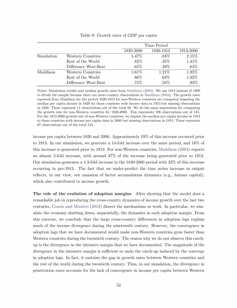
Table 9: Growth rates of GDP per capita

Time Period1820-2000 1820-1913 1913-2000

Simulation Western Countries 1.47% .84% 2.15%Rest of the World .82% .35% 1.31%Difference West-Rest .65% .49% .84%

Maddison Western Countries 1.61% 1.21% 1.95%Rest of the World .86% .63% 1.02%Difference West-Rest .75% .58% .93%

Notes: Simulation results and median growth rates from Maddison (2004). We use 1913 instead of 1900to divide the sample because there are more country observations in Maddison (2004). The growth ratesreported from Maddison for the period 1820-1913 for non-Western countries are computed imputing themedian per capita income in 1820 for those countries with income data in 1913 but missing observationsin 1820. These represent 11 observations out of the total 50. We do the same imputation for computingthe growth rate for non-Western countries for 1820-2000. This represents 106 observations out of 145.For the 1913-2000 growth rate of non-Western countries, we impute the median per capita income in 1913to those countries with income per capita data in 2000 but missing observations in 1913. These represent67 observations out of the total 145.

income per capita between 1820 and 2000. Approximately 19% of this increase occurred prior

to 1913. In our simulation, we generate a 14-fold increase over the same period, and 16% of

this increase is generated prior to 1913. For non-Western countries, Maddison (2004) reports

an almost 5-fold increase, with around 37% of the increase being generated prior to 1913.

Our simulation generates a 4.3-fold increase in the 1820-2000 period with 32% of this increase

occurring in pre-1913. The fact that we under-predict the time series increase in output

reflects, in our view, our omission of factor accumulation dynamics (e.g., human capital),

which also contributed to income growth.

The role of the evolution of adoption margins After showing that the model does a

remarkable job in reproducing the cross-country dynamics of income growth over the last two

centuries, Comin and Mestieri (2013) dissect the mechanisms at work. In particular, we sim-

ulate the economy shutting down, sequentially, the dynamics in each adoption margin. From

this exercise, we conclude that the large cross-country differences in adoption lags explain

much of the income divergence during the nineteenth century. However, the convergence in

adoption lags that we have documented would make non-Western countries grow faster than

Western countries during the twentieth century. The reason why we do not observe this catch-

up is the divergence in the intensive margin that we have documented. The magnitude of the

divergence in the intensive margin is sufficient to undo the catch-up induced by the converge

in adoption lags. In fact, it sustains the gap in growth rates between Western countries and

the rest of the world during the twentieth century. Thus, in our simulation, the divergence in

penetration rates accounts for the lack of convergence in income per capita between Western

52

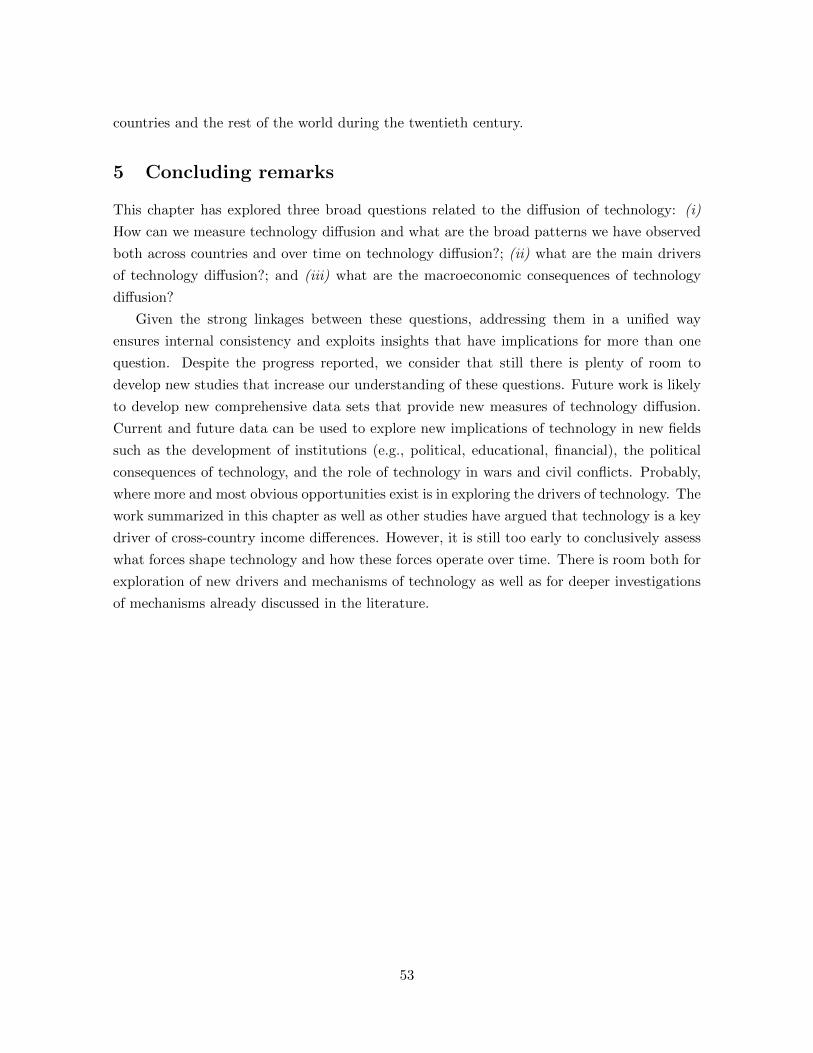
countries and the rest of the world during the twentieth century.

5 Concluding remarks

This chapter has explored three broad questions related to the diffusion of technology: (i)

How can we measure technology diffusion and what are the broad patterns we have observed

both across countries and over time on technology diffusion?; (ii) what are the main drivers

of technology diffusion?; and (iii) what are the macroeconomic consequences of technology

diffusion?

Given the strong linkages between these questions, addressing them in a unified way

ensures internal consistency and exploits insights that have implications for more than one

question. Despite the progress reported, we consider that still there is plenty of room to

develop new studies that increase our understanding of these questions. Future work is likely

to develop new comprehensive data sets that provide new measures of technology diffusion.

Current and future data can be used to explore new implications of technology in new fields

such as the development of institutions (e.g., political, educational, financial), the political

consequences of technology, and the role of technology in wars and civil conflicts. Probably,

where more and most obvious opportunities exist is in exploring the drivers of technology. The

work summarized in this chapter as well as other studies have argued that technology is a key

driver of cross-country income differences. However, it is still too early to conclusively assess

what forces shape technology and how these forces operate over time. There is room both for

exploration of new drivers and mechanisms of technology as well as for deeper investigations

of mechanisms already discussed in the literature.

53

References

Acemoglu, D., Johnson, S. and Robinson, J. A. (2002). Reversal of fortune: Geography

and institutions in the making of the modern world income distribution. The Quarterly

Journal of Economics, 117 (4), 1231–1294.

—, — and — (2005). Institutions as a fundamental cause of long-run growth. In P. Aghion

and S. Durlauf (eds.), Handbook of Economic Growth, Handbook of Economic Growth, vol. 1,

6, Elsevier, pp. 385–472.

— and Robinson, J. A. (2000). Why did the west extend the franchise? democracy, inequal-

ity, and growth in historical perspective. The Quarterly Journal of Economics, 115 (4),

1167–1199.

Aghion, P. and Howitt, P. (1992). A model of growth through creative destruction. Econo-

metrica, 60 (2), 323–51.

Alexopoulos, M. (2011). Read all about it!! what happens following a technology shock?

American Economic Review, 101 (4), 1144–79.

Arellano, M. and Bond, S. (1991). Some tests of specification for panel data: Monte carlo

evidence and an application to employment equations. Review of Economic Studies, 58 (2),

277–97.

Arrow, K. J. (1962). The economic implications of learning by doing. The Review of Eco-

nomic Studies, 29 (3), 155–173.

Arthur, W. B. (1989). Competing technologies, increasing returns, and lock-in by historical

events. Economic Journal, 99, 116–131.

Ashraf, Q. and Galor, O. (2013). The ’out of africa’ hypothesis, human genetic diversity,

and comparative economic development. American Economic Review, 103 (1), 1–46.

Bandiera, O. and Rasul, I. (2006). Social networks and technology adoption in northern

mozambique. Economic Journal, 116 (514), 869–902.

Banerjee, A. (1992). A simple model of herd behavior. Quarterly Journal of Economics,

107 (3), 797–817.

Barlevy, G. (2007). On the cyclicality of research and development. American Economic

Review, 97 (4), 1131–1164.

Barro, R. J. and Sala-i-Martin, X. (2003). Economic Growth, 2nd Edition. The MIT

Press.

54

Basu, S. (1996). Procyclical productivity: Increasing returns or cyclical utilization? The

Quarterly Journal of Economics, 111 (3), 719–51.

— and Fernald, J. G. (1997). Returns to scale in u.s. production: Estimates and implica-

tions. Journal of Political Economy, 105 (2), 249–283.

Benhabib, J. and Spiegel, M. M. (1994). The role of human capital in economic develop-

ment evidence from aggregate cross-country data. Journal of Monetary Economics, 34 (2),

143–173.

— and — (2005). Human capital and technology diffusion. In P. Aghion and S. Durlauf (eds.),

Handbook of Economic Growth, Handbook of Economic Growth, vol. 1, 13, Elsevier, pp.

935–966.

Besley, T. and Case, A. (1995). Does electoral accountability affect economic policy

choices? evidence from gubernatorial term limits. The Quarterly Journal of Economics,

110 (3), 769–98.

Bockstette, V., Chanda, A. and Putterman, L. (2002). States and markets: The

advantage of an early start. Journal of Economic Growth, 7 (4), 347–69.

Burnside, C., Eichenbaum, M. and Rebelo, S. (1995). Capital utilization and returns

to scale. In NBER Macroeconomics Annual 1995, Volume 10, NBER Chapters, National

Bureau of Economic Research, Inc, pp. 67–124.

Caballero, R. J., Hoshi, T. and Kashyap, A. K. (2008). Zombie lending and depressed

restructuring in japan. American Economic Review, 98 (5), 1943–77.

Caselli, F. (1999). Technological revolutions. American Economic Review, 89 (1), 78–102.

— and Coleman, W. J. (2001). Cross-country technology diffusion: The case of computers.

American Economic Review, 91 (2), 328–335.

Chari, V. V. and Hopenhayn, H. (1991). Vintage human capital, growth, and the diffusion

of new technology. Journal of Political Economy, 99 (6), 1142–65.

Clark, G. (1987). Why isn’t the whole world developed: Lessons from the cotton mills. The

Journal of Economic History, 47 (1), 141–173.

Coe, D. T. and Helpman, E. (1995). International r&d spillovers. European Economic

Review, 39 (5), 859–887.

Cogley, T. and Nason, J. M. (1995). Output dynamics in real-business-cycle models.

American Economic Review, 85 (3), 492–511.

55

Comin, D. (2009). On the integration of growth and business cycles. Empirica, 36 (2).

— (2011). An exploration of the japanese slowdown during the 1990s. In A. K. K.

Koichi Hamada and D. E. Weinstein (eds.), Japans Bubble, Deflation, and Long-term Stag-

nation, vol. 1, MIT Press, pp. 375–398.

—, Dmitriev, M. and Rossi-Hansberg, E. (2013). The Spatial Diffusion of Technology.

Tech. rep.

—, Easterly, W. and Gong, E. (2010). Was the wealth of nations determined in 1000 bc?

American Economic Journal: Macroeconomics, 2 (3), 65–97.

— and Gertler, M. (2006). Medium-term business cycles. The American Economic Review,

96 (3), 523–551.

—, — and Santacreu, A. M. (2009a). Technology Innovation and Diffusion as Sources of

Output and Asset Price Fluctuations. NBER Working Papers 15029, National Bureau of

Economic Research, Inc.

— and Hobijn, B. (2004). Cross-country technology adoption: Making theory face the facts.

Journal of Monetary Economics, (51), 39–83.

— and — (2007). Implementing Technology. Tech. rep.

— and — (2009a). The CHAT Dataset. Working Paper 15319, National Bureau of Economic

Research.

— and — (2009b). Lobbies and technology diffusion. Review of Economics and Statistics,

91 (2), 229–244.

— and — (2010). An exploration of technology diffusion. American Economic Review,

100 (5), 2031–59.

—, — and Rovito, E. (2006). Five Facts You Need to Know About Technology Diffusion.

NBER Working Papers 11928, National Bureau of Economic Research, Inc.

—, — and — (2008a). A new approach to measuring technology with an application to the

shape of the diffusion curves. The Journal of Technology Transfer, 33 (2), 187–207.

—, — and — (2008b). Technology usage lags. Journal of Economic Growth, 13 (4), 237–256.

—, Loayza, N., Pasha, F. and Serven, L. (2009b). Medium Term Business Cycles in De-

veloping Countries. NBER Working Papers 15428, National Bureau of Economic Research,

Inc.

56

— and Mestieri, M. (2010). An intensive exploration of technology adoption. NBER Work-

ing Paper 16379.

— and — (2013). If Technology Has Arrived Everywhere, why has Income Diverged? Working

Paper 19010, National Bureau of Economic Research.

—, Trumbull, J. G. and Yang, K. (2012). Fraunhofer: Innovation in Germany. Tech.

Rep. 711-02, Harvard Business School Case.

Conley, T. G. and Udry, C. R. (2010). Learning about a new technology: Pineapple in

ghana. American Economic Review, 100 (1), 35–69.

Cox, W. M. and Alm, R. (1996). The economy at light speed: technology and growth in

the information age and beyond. Annual Report, pp. 2–17.

Crafts, N. (1997). Endogenous growth: Lessons for and from economic history. In D. Kreps

and K. F. Wallis (eds.), Advances in Economics and Econometrics: Theory and Applica-

tions, vol. 2, CUP, pp. 38–78.

Davies, S. (1979). The Diffusion of Process Innovations. Cambridge University Press.

Diamond, J. (1999). Guns, germs, and steel: the fates of human societies. Norton paperback,

W W Norton & Company Incorporated.

Dixon, R. (1980). Hybrid corn revisited. Econometrica, 48, 145–146.

Dupas, P. (2009). What matters (and what does not) in households’ decision to invest in

malaria prevention? American Economic Review, 99 (2), 224–30.

Erosa, A., Koreshkova, T. and Restuccia, D. (2010). How important is human capital?

a quantitative theory assessment of world income inequality. Review of Economic Studies,

77 (4), 1421–1449.

Evenson, R. E. and Gollin, D. (2003). Assessing the impact of the green revolution, 1960

to 2000. Science, 300 (5620), 758–762.

Fatas, A. (2000). Endogenous growth and stochastic trends. Journal of Monetary Economics,

45 (1), 107–128.

Ferejohn, J. (1986). Incumbent performance and electoral control. Public Choice, 50 (1),

5–25.

Feyrer, J. (2009a). Distance, Trade, and Income The 1967 to 1975 Closing of the Suez

Canal as a Natural Experiment. NBER Working Papers 15557, National Bureau of Eco-

nomic Research, Inc.

57

— (2009b). Trade and Income – Exploiting Time Series in Geography. NBER Working Papers

14910, National Bureau of Economic Research, Inc.

Foster, A. D. and Rosenzweig, M. R. (1995). Learning by doing and learning from others:

Human capital and technical change in agriculture. Journal of Political Economy, 103 (6),

1176–1209.

— and — (2010). Microeconomics of technology adoption. Annual Review of Economics,

2 (1), 395–424.

Frankel, J. A. and Romer, D. H. (1999). Does trade cause growth? American Economic

Review, 89 (3), 379–399.

Galı, J. (1999). Technology, employment, and the business cycle: Do technology shocks

explain aggregate fluctuations? American Economic Review, 89 (1), 249–271.

Geroski, P. (2000). Models of technology diffusion. Research Policy, 29, 603–625.

Gort, M. and Klepper, S. (1982). Time paths in the diffusion of product innovations.

Economic Journal, 92 (367), 630–53.

Griliches, Z. (1957). Hybrid corn: an exploration in the economics of technological change.

Econometrica, 25 (4), 501–522.

— (1990). Patent statistics as economic indicators: A survey. Journal of Economic Literature,

28 (4), 1661–1707.

Guiso, L., Sapienza, P. and Zingales, L. (2008). Alfred marshall lecture social capital as

good culture. Journal of the European Economic Association, 6 (2-3), 295–320.

Hannan, M. T. and Freeman, J. (1989). Organizations and social structure. Organizational

Ecology, pp. 3–27.

James S. Coleman, E. K. and Menzel, H. (1966). Medical innovation: A diffusion study.

Bobbs-Merrill Co.

Johansen, L. (1959). Substitution versus fixed production coefficients in the theory of eco-

nomic growth: A synthesis. Econometrica, pp. 157–176.

Karshenas, M. and Stoneman, P. L. (1993). Rank, stock, order, and epidemic effects

in the diffusion of new process technologies: An empirical model. The RAND Journal of

Economics, pp. 503–528.

Keller, W. (2004). International technology diffusion. Journal of Economic Literature,

42 (3), 752–782.

58

Kunicova, J. and Rose-Ackerman, S. (2005). Electoral rules and constitutional structures

as constraints on corruption. British Journal of Political Science, 35, 573–606.

Kydland, F. E. and Prescott, E. C. (1982). Time to build and aggregate fluctuations.

Econometrica, 50 (6), 1345–70.

Levin, S., Levin, S. and Meisel, J. (1987). A dynamic analysis of the adoption of a new

technology: the case of optical scanners. Review of Economics and Statistics, (69), 12–17.

Lucas, R. E., Buera, F. J. and Alvarez, F. (2011). Trade and Idea Flows. 2011 Meeting

Papers 984, Society for Economic Dynamics.

Maddison, A. (2004). Contours of the world economy and the art of macro-measurement

1500-2001. Ruggles Lecture.

Mansfield, E. (1961). Technical change and the rate of imitation. Econometrica, 29 (4),

741–766.

— (1963). The speed of response of firms to new technologies. Quarterly Journal of Economics,

29 (77), 290–311.

— (1968). Industrial Research and Technological Innovation. W.W. Norton, New York.

Metcalfe, J. S. (1981). Impulse and diffusion in the study of technical change. Futures,

13 (5), 347–359.

— (1998). Evolutionary Economics and Creative Destruction. Routledge.

Mokyr, J. (1990). The Lever of Riches: Technological Creativity and Economic Progress.

Oxford paperbacks, Oxford University Press, USA.

Myerson, R. B. (1993). Effectiveness of electoral systems for reducing government corrup-

tion: A game-theoretic analysis. Games and Economic Behavior, 5 (1), 118–132.

Nelson, R. R. and Phelps, E. S. (1966). Investment in humans, technological diffusion

and economic growth. American Economic Review, 56 (1/2), 69–75.

Norbin, S. (1993). The relation between price and marginal cost in u.s. industry: A contra-

diction. Journal of Political Economy, 101 (6), 1149–64.

Olson, M. (1982). The Rise and Decline of Nations: Economic Growth, Stagflation and

Social Rigidities. Yale university.

Peregrine, P. (2003). Atlas of cultural evolution. In World Cultures, 14, J.P. Gray.

59

Perla, J., Tonetti, C. and Waugh, M. E. (2012). Equilibrium Technology Diffusion,

Trade and Growth. Tech. rep., Mimeo.

Persson, T., Roland, G. and Tabellini, G. (2000). Comparative politics and public

finance. Journal of Political Economy, 108 (6), 1121–1161.

—, Tabellini, G. and Trebbi, F. (2003). Electoral rules and corruption. Journal of the

European Economic Association, 1 (4), 958–989.

Porter, M. E. (1998). ”clusters and the new economics of competition. Harvard Business

Review, pp. 77–90.

Putterman, L. and Weil, D. N. (2010). Post-1500 population flows and the long-run

determinants of economic growth and inequality. The Quarterly Journal of Economics,

125 (4), 1627–1682.

Riddell, W. C. and Song, X. (2012). The Role of Education in Technology Use and Adop-

tion: Evidence from the Canadian Workplace and Employee Survey. IZA Discussion Papers

6377, Institute for the Study of Labor (IZA).

Romeo, A. (1975). Inter-industry and inter-firm differences in the rate of diffusion of an

innovation. Review of Economics and Statistics, 57, 311–316.

Romer, P. M. (1990). Endogenous technological change. Journal of Political Economy,

98 (5), S71–102.

Rose, N. and Joskow, P. (1990). The diffusion of new technologies: evidence from the

electric utility industry. The Rand Journal of Economics, (21), 354–373.

Sachs, J. and Warner, A. (1995). Economic Reform and the Progress of Global Integra-

tion. Harvard Institute of Economic Research Working Papers 1733, Harvard - Institute of

Economic Research.

Santos, M. S. and Iraola, M. A. (2010). Long-Term Asset Price Volatility and Macroe-

conomic Fluctuations. 2010 Meeting Papers 374, Society for Economic Dynamics.

Scherer, F. (1981). Using linked patent and R&D data to measure inter-industry technology

flows. In Z. Griliches (ed.), R&D, Patents, and Productivity, University of Chicago Press,

pp. 417–464.

Schmookler, J. (1966). Invention and economic growth. Harvard University Press.

Seshadri, A. and Manuelli, R. (2005). Human Capital and the Wealth of Nations. 2005

Meeting Papers 56, Society for Economic Dynamics.

60

Skinner, J. and Staiger, D. (2007). Technology adoption from hybrid corn to beta-blockers.

In Hard-to-Measure Goods and Services: Essays in Honor of Zvi Griliches, NBER Chapters,

National Bureau of Economic Research, Inc, pp. 545–570.

Solow, R. M. (1956). A contribution to the theory of economic growth. The Quarterly

Journal of Economics, 70 (1), 65–94.

— (1960). Investment and technical progress. In S. K. K. Arrow and P. Suppes (eds.), Math-

ematical Methods in the Social Sciences, vol. 1, Stanford University Press, pp. 89–104.

Spolaore, E. and Wacziarg, R. (2009). The diffusion of development. The Quarterly

Journal of Economics, 124 (2), 469–529.

Stoneman, P. (1981). Intra-firm diffusion, bayesian learning and profitability. Economic

Journal, 91 (362), 375–88.

— (1983). The economic analysis of technological change. Oxford University Press Oxford.

— (1987). The economic analysis of technology policy. Clarendon Press Oxford.

— et al. (1995). Handbook of the economics of innovation and technological change. Blackwell

Oxford.

Tabellini, G. (2007). Institutions and Culture. Working Papers 330, IGIER (Innocenzo

Gasparini Institute for Economic Research), Bocconi University.

Thirtle, C. and Ruttan, V. (1987). The Role of Demand and Supply in the Generation

and Diffusion of Technical Change. Fundamentals of Pure and Applied Economics Series,

Harwood Academic Publications.

Vickery, G. and Northcott, J. (1995). Diffusion of microelectronics and advanced man-

ufacturing technology: A review of national surveys. Economics of Innovation and New

Technology, 3 (3-4), 253–276.

A Description of Technologies used to Estimate Diffusion Curves

The twenty-five particular technology measures, organized by broad category (transportation,

communication, IT, industrial, agricultural and medical) are described below.

Transportation

61

1. Steam and motor ships: Gross tonnage (above a minimum weight) of steam and

motor ships in use at midyear. Invention year: 1788; the year the first (U.S.) patent

was issued for a steam boat design.

2. Railways - Passengers: Passenger journeys by railway in passenger-KM.

Invention year: 1825; the year of the first regularly schedule railroad service to carry

both goods and passengers.

3. Railways - Freight: Metric tons of freight carried on railways (excluding livestock

and passenger baggage).

Invention year: 1825; same as passenger railways.

4. Cars: Number of passenger cars (excluding tractors and similar vehicles) in use. Inven-

tion year: 1885; the year Gottlieb Daimler built the first vehicle powered by an internal

combustion engine.

5. Trucks: Number of commercial vehicles, typically including buses and taxis (excluding

tractors and similar vehicles), in use. Invention year: 1885; same as cars.

6. Tractor: Number of wheel and crawler tractors (excluding garden tractors) used in agri-

culture. Invention year: 1892; John Froelich invented and built the first gasoline/petrol-

powered tractor.

7. Aviation - Passengers: Civil aviation passenger-KM traveled on scheduled services

by companies registered in the country concerned. Invention year: 1903; The year the

Wright brothers managed the first successful flight.

8. Aviation - Freight: Civil aviation ton-KM of cargo carried on scheduled services by

companies registered in the country concerned. Invention year: 1903; same as aviation

- passengers.

Communication and IT

1. Telegraph: Number of telegrams sent. Invention year: 1835; year of invention of

telegraph by Samuel Morse at New York University.

2. Mail: Number of items mailed/received, with internal items counted once and cross-

border items counted once for each country. Invention year: 1840; the first modern

postage stamp, Penny Black, was released in Great Britain.

3. Telephone: Number of mainline telephone lines connecting a customer’s equipment

to the public switched telephone network. Invention year: 1876; year of invention of

telephone by Alexander Graham Bell.

62

4. Cellphone: Number of users of portable cell phones. Invention year: 1973; first call

from a portable cellphone.

5. Personal computers: Number of self-contained computers designed for use by one

person. Invention year: 1973; first computer based on a microprocessor.

6. Internet users: Number of people with access to the worldwide network. Invention

year: 1983; introduction of TCP/IP protocol.

Industrial

1. Spindles: Number of mule and ring spindles in place at year end. Invention year: 1779;

Spinning Mule invented by Samuel Crompton.

2. Synthetic Fiber: Weight of synthetic (noncellulosic) fibers used in spindles Invention

year: 1924; Invention of rayon.

3. Steel: Total tons of crude steel production (in metric tons). This measure includes steel

produced using Bessemer and Open Earth furnaces. Invention year: 1855; William Kelly

receives the first patent for a steel making process (pneumatic steel making).

4. Electric Arc Furnaces: Crude steel production (in metric tons) using electric arc

furnaces. Invention year: 1907; invention of the Electric Arc Furnace.

5. Blast Oxygen Furnaces: Crude steel production (in metric tons) in blast oxygen

furnaces (a process that replaced Bessemer and OHF processes). Invention year: 1950;

invention of Blast Oxygen Furnace.

6. Electricity: Gross output of electric energy (inclusive of electricity consumed in power

stations) in Kw-Hr. Invention year: 1882; first commercial power station on Pearl Street

in New York City.

Agricultural

1. Fertilizer: Metric tons of fertilizer consumed. Aggregate of 25 individual types, cor-

responding to broadly Ammonia and Phosphates. Invention year: 1910; Haber-Bosch

process to produce ammonia is patented in 1910.

2. Harvester: Number of selfpropelled machines that reap and thresh in one operation.

Invention year: 1912; The Holt Manufacturing Company of California produces a self-

propelled harvester. Subsequently, a selfpropelled machine that reaps and threshes in

63

one operation appears.

Medical

1. Kidney Transplant: Number of kidney transplants performed. Invention year: 1954;

Joseph E. Murray and his colleagues at Peter Bent Brigham Hospital in Boston per-

formed the first successful kidney transplant.

2. Liver Transplant: Number of liver transplants performed. Invention year: 1963; Dr.

Thomas Starzl performs the first successful liver transplant in the United States.

3. Heart Transplant: Number of heart transplants performed Invention year: 1968;

Adrian Kantrowitz performed the first pediatric heart transplant in the world on De-

cember 6, 1967 at Maimonides Hospital.

B Additional Tables

64

Tab

le10

:C

orre

lati

ons

and

join

tsa

mp

lesi

zes

Inven

-st

.T

ech

nolo

gy

tion

Yea

rO

bs.

Mea

nM

edia

nd

ev.

IQR

12

34

56

78

910

11

12

13

14

15

16

Rea

lG

DP

1950

138

149

128

93

128

0.9

30.8

20.7

50.7

70.7

50.7

50.7

70.7

10.7

10.7

50.6

10.7

0.6

30.7

10.6

3R

eal

GD

P1970

138

118

114

79

114

138

0.9

0.8

20.7

80.8

30.8

60.8

20.7

70.7

90.8

0.6

50.7

60.7

50.7

60.6

6R

eal

GD

P1990

164

113

94

82

119

138

138

0.9

40.7

40.8

0.8

90.8

60.8

0.8

10.7

50.6

60.7

70.7

30.6

80.6

1R

eal

GD

P2000

164

122

105

89

119

138

138

164

0.6

90.7

50.8

30.8

70.8

0.8

20.7

0.6

50.7

50.6

80.6

50.5

8E

lect

rici

ty1882

1950

99

46

48

20

29

96

96

97

97

0.9

40.8

90.8

10.8

20.7

20.9

0.6

60.7

50.8

0.8

80.8

1E

lect

rici

ty1882

1970

124

52

59

25

37

119

119

121

121

99

0.9

40.8

40.8

50.8

0.8

90.6

70.7

70.7

90.8

70.7

7E

lect

rici

ty1882

1990

127

58

57

28

46

120

120

126

126

97

121

0.8

60.8

60.8

20.8

50.6

80.8

0.8

20.8

0.7

Inte

rnet

1983

2002

123

98

56

101

101

120

120

81

99

103

0.8

90.8

60.8

10.7

40.8

10.7

40.7

80.6

9P

Cs

1973

2002

127

18

20

76

108

108

124

124

86

107

111

110

0.8

0.8

90.7

60.8

40.7

50.8

30.7

4C

ellp

hon

es1973

2002

145

88

611

118

118

142

142

93

116

120

122

127

0.7

60.7

70.7

90.6

90.7

20.5

8T

elep

hon

es1876

1970

108

63

70

23

15

104

104

106

106

90

106

105

90

95

102

0.7

0.7

90.8

30.9

30.8

4A

vi.

Carg

o1903

1990

96

27

30

16

23

92

92

95

95

76

93

95

79

88

92

83

0.8

90.6

80.6

90.5

1A

vi.

Pass

.1903

1990

102

34

38

14

21

98

98

101

101

81

99

101

83

92

97

88

96

0.8

30.7

50.6

Tru

cks

1885

1990

98

59

67

18

26

97

97

98

98

78

96

96

81

84

94

86

78

83

0.8

20.6

6C

ars

1885

1990

127

66

74

20

14

106

106

127

127

81

100

105

102

103

119

92

81

86

97

0.8

4T

ract

ors

1894

1970

130

47

52

16

11

124

124

128

128

97

121

123

105

113

123

105

95

101

96

107

Note

:st

.dev

.is

standard

dev

iati

on.

IQR

isth

ein

terq

uart

ile

range.

Inth

eco

rrel

ati

ons

and

join

tsa

mple

ssi

zes

part

,th

enum

ber

sab

ove

the

dia

gonal

are

the

corr

elati

ons

and

the

num

ber

sb

elow

the

dia

gonal

are

the

sam

ple

size

on

whic

hth

eco

rrel

ati

ons

are

base

d

65

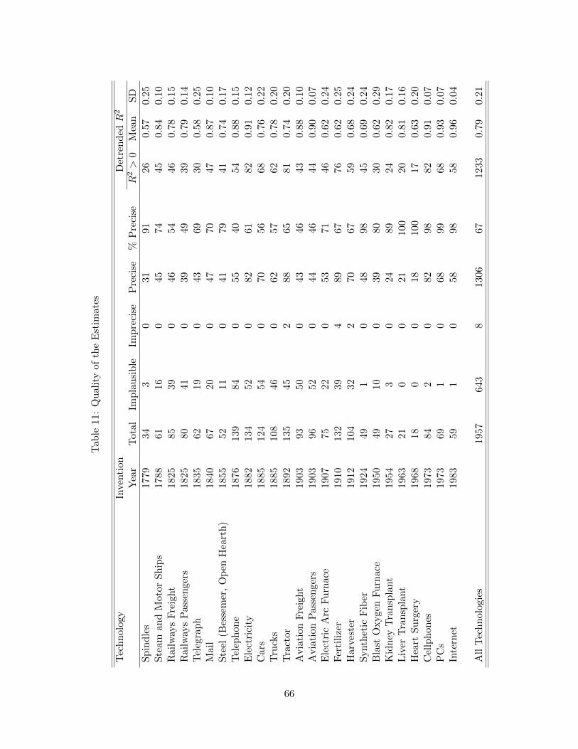
Tab

le11

:Q

ual

ity

ofth

eE

stim

ates

Tec

hn

olog

yIn

venti

onD

etre

nd

edR

2

Yea

rT

otal

Imp

lau

sib

leIm

pre

cise

Pre

cise

%P

reci

seR

2>

0M

ean

SD

Sp

ind

les

1779

343

031

9126

0.5

70.2

5S

team

and

Mot

orS

hip

s17

8861

160

4574

45

0.8

40.1

0R

ailw

ays

Fre

ight

1825

8539

046

5446

0.7

80.1

5R

ailw

ays

Pas

sen

gers

1825

8041

039

4939

0.7

90.1

4T

eleg

rap

h18

3562

190

4369

30

0.5

80.2

5M

ail

1840

6720

047

7047

0.8

70.1

0S

teel

(Bes

sem

er,

Op

enH

eart

h)

1855

5211

041

7941

0.7

40.1

7T

elep

hon

e18

7613

984

055

4054

0.8

80.1

5E

lect

rici

ty18

8213

452

082

6182

0.9

10.1

2C

ars

1885

124

540

7056

68

0.7

60.2

2T

ruck

s18

8510

846

062

5762

0.7

80.2

0T

ract

or18

9213

545

288

6581

0.7

40.2

0A

via

tion

Fre

ight

1903

9350

043

4643

0.8

80.1

0A

via

tion

Pas

senge

rs19

0396

520

4446

44

0.9

00.0

7E

lect

ric

Arc

Fu

rnac

e19

0775

220

5371

46

0.6

20.2

4F

erti

lize

r19

1013

239

489

6776

0.6

20.2

5H

arve

ster

1912

104

322

7067

59

0.6

80.2

4S

ynth

etic

Fib

er19

2449

10

4898

45

0.6

90.2

4B

last

Oxyge

nF

urn

ace

1950

4910

039

8030

0.6

20.2

9K

idn

eyT

ran

spla

nt

1954

273

024

8924

0.8

20.1

7L

iver

Tra

nsp

lant

1963

210

021

100

20

0.8

10.1

6H

eart

Su

rger

y19

6818

00

1810

017

0.6

30.2

0C

ellp

hon

es19

7384

20

8298

82

0.9

10.0

7P

Cs

1973

691

068

9968

0.9

30.0

7In

tern

et19

8359

10

5898

58

0.9

60.0

4

All

Tec

hn

olog

ies

1957

643

813

0667

1233

0.7

90.2

1

66