EWO Seminar

“Using IMPRESS for Supply-Chain Scenario-Based Optimization”

Industrial Algorithms LLC.Jeff Kelly & Alkis Vazacopoulos

4/18/2013Copyright, Industrial Algorithms LLC

Agenda• IAL Introduction.• What is IMPRESS?• Jet Fuel Supply Chain & Why it’s Complex.• Scenario Generation.IMPRESS is a new industrial modeling and presolving system which can represent many types of optimization and simulation problems found in the process industries including planning, scheduling, control and data reconciliation problems. It is designed to handle large-scale systems given its efficient sparse data memory and manipulation techniques and is well-suited for both discrete and nonlinear models. IMPRESS embeds both MILP and NLP state-of-the-art solvers and is also capable of binding to meta-heuristics. IMPRESS is based on two core fundamentals: 1) the flowsheet can be represented using our unit-operation-port-state superstructure (UOPSS) which extends the well-known STN and RTN to both batch and continuous processes with limited connectivity as well as to dimensional processes and 2) the variables can be categorized into our quantity, logic and quality phenomena (QLQP) i.e., flows, holdups, setups, startups, properties, conditions, etc. The time digitization model for IMPRESS is discrete-time for logistics problems (quantity times logic) and what we call distributed-time for quality problems (quantity times quality) i.e., using a global or common time-grid but with equal or unequal time-periods which is common in planning.

To highlight IMPRESS, we detail a small jet fuel supply-chain problem which includes an oil-refinery producing several products including swing-cuts, a rail-road transportation system with tankers and an airport with on-site inventory. We also consider in this example the possibility of arbitrary uncertain situations such as unit-operation availability and supply/demand variability in terms of quantity, logic and timing variations. Each configured scenario is contained as a separate problem instance with essentially time-varying capacity parameters manifesting the uncertainties. The scenarios can be run serially or in-parallel on multi-core computers where each solution can be interrogated by interfacing an ASCII file or interactively using API's in any computer programming language. 2

Our Mission Statement • To provide advanced modeling and solving

tools for developing and deploying industrial applications in the decision-making and data-mining areas.

• Our targets are: – Operating companies in the process industries.– Consulting service providers.– Application software providers.

Our Focus• IAL develops and markets IMPRESS, the

world’s leading software platform for flowsheetoptimization in both off and on-line environments.

• IAL provides in-house training for customers along with complete software support and consulting.

• IAL provides Industrial Modeling Frameworks (IMF’s) for many problem types.

4

Our Industrial Modeling Frameworks (IMF’s)

• Process industry business problems are complex hence an IMF provides a pre-project or pre-solution advantage.

• An IMF embeds intellectual-property and know-how related to the process’s flowsheet modeling as well as its problem-solving methodology.

Our Modeling Environment IMPRESS• IMPRESS stands for “Industrial Modeling & PRE-

Solving System” and is our proprietary platform.• You can “interface”, “interact”, “model” and

“solve” any production-chain, supply-chain, demand-chain and/or value-chain optimization problem.

• IMPRESS so far has been applied to: – Process Scheduling– Production Planning– Pipeline & Marine Shipping – Energy Management

6

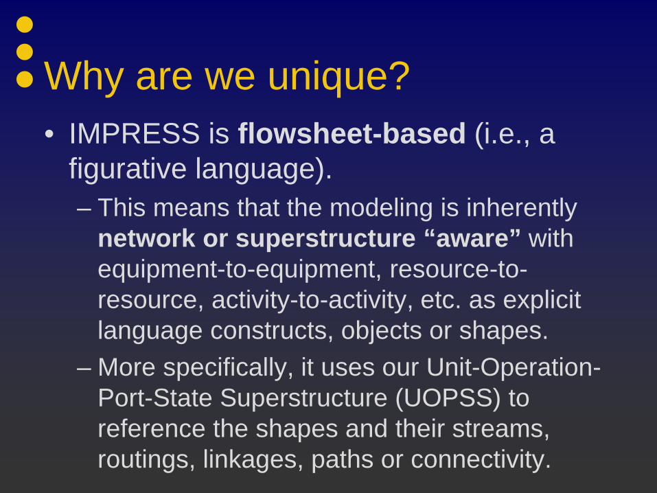
Why are we unique? • IMPRESS is flowsheet-based (i.e., a

figurative language). – This means that the modeling is inherently

network or superstructure “aware” with equipment-to-equipment, resource-to-resource, activity-to-activity, etc. as explicit language constructs, objects or shapes.

– More specifically, it uses our Unit-Operation-Port-State Superstructure (UOPSS) to reference the shapes and their streams, routings, linkages, paths or connectivity.

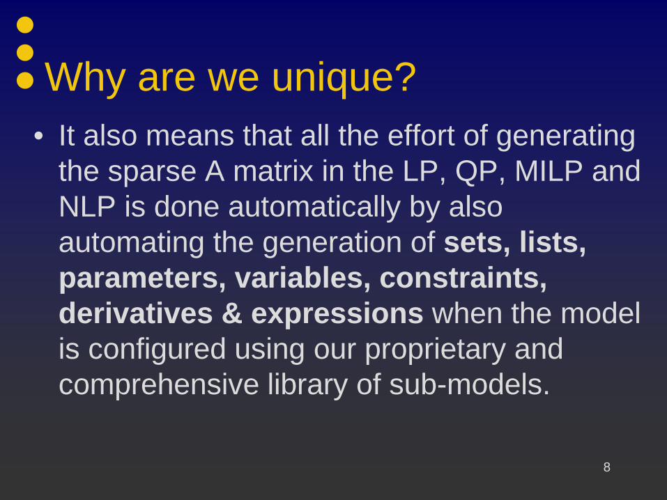
Why are we unique? • It also means that all the effort of generating

the sparse A matrix in the LP, QP, MILP and NLP is done automatically by also automating the generation of sets, lists, parameters, variables, constraints, derivatives & expressions when the model is configured using our proprietary and comprehensive library of sub-models.

8

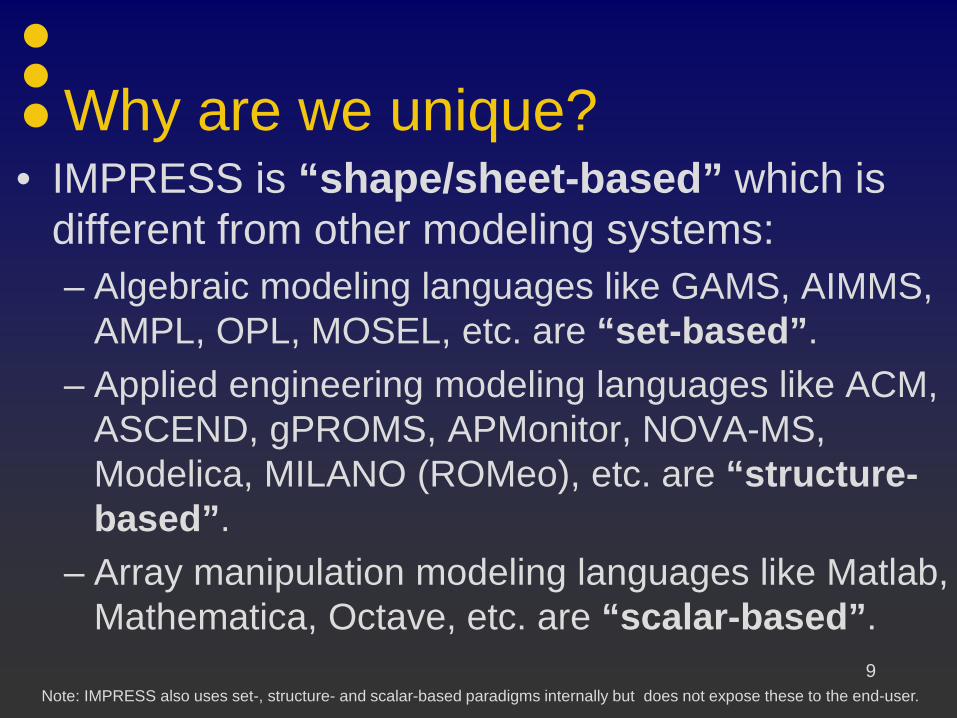
Why are we unique? • IMPRESS is “shape/sheet-based” which is

different from other modeling systems:– Algebraic modeling languages like GAMS, AIMMS,

AMPL, OPL, MOSEL, etc. are “set-based”.– Applied engineering modeling languages like ACM,

ASCEND, gPROMS, APMonitor, NOVA-MS, Modelica, MILANO (ROMeo), etc. are “structure-based”.

– Array manipulation modeling languages like Matlab, Mathematica, Octave, etc. are “scalar-based”.

Note: IMPRESS also uses set-, structure- and scalar-based paradigms internally but does not expose these to the end-user. 9

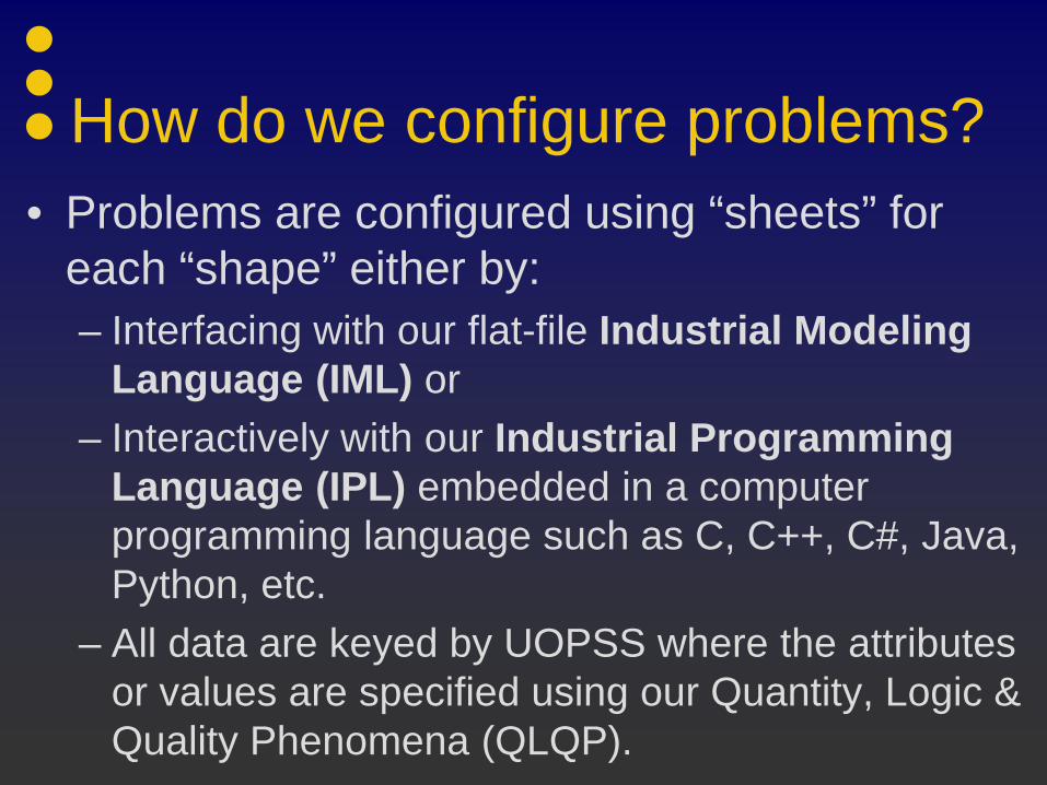
• Problems are configured using “sheets” for each “shape” either by:– Interfacing with our flat-file Industrial Modeling

Language (IML) or– Interactively with our Industrial Programming

Language (IPL) embedded in a computer programming language such as C, C++, C#, Java, Python, etc.

– All data are keyed by UOPSS where the attributes or values are specified using our Quantity, Logic & Quality Phenomena (QLQP).

How do we configure problems?

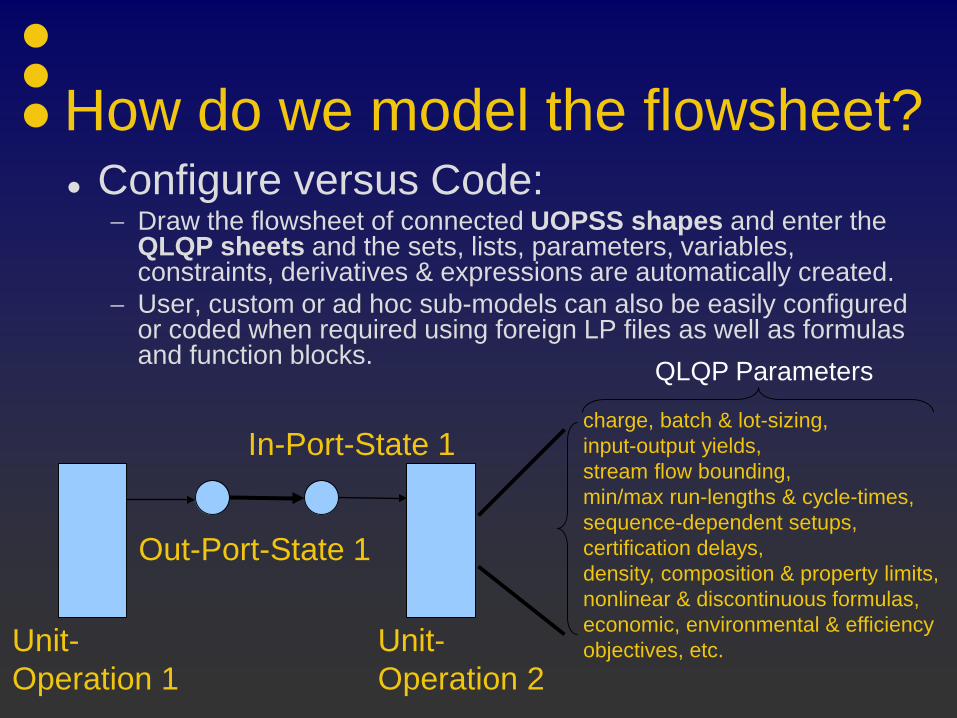
Configure versus Code:− Draw the flowsheet of connected UOPSS shapes and enter the

QLQP sheets and the sets, lists, parameters, variables, constraints, derivatives & expressions are automatically created.

− User, custom or ad hoc sub-models can also be easily configured or coded when required using foreign LP files as well as formulas and function blocks.

Unit-Operation 1

Unit-Operation 2

Out-Port-State 1

In-Port-State 1charge, batch & lot-sizing,input-output yields,stream flow bounding,min/max run-lengths & cycle-times, sequence-dependent setups,certification delays,density, composition & property limits,nonlinear & discontinuous formulas,economic, environmental & efficiency objectives, etc.

How do we model the flowsheet?

QLQP Parameters

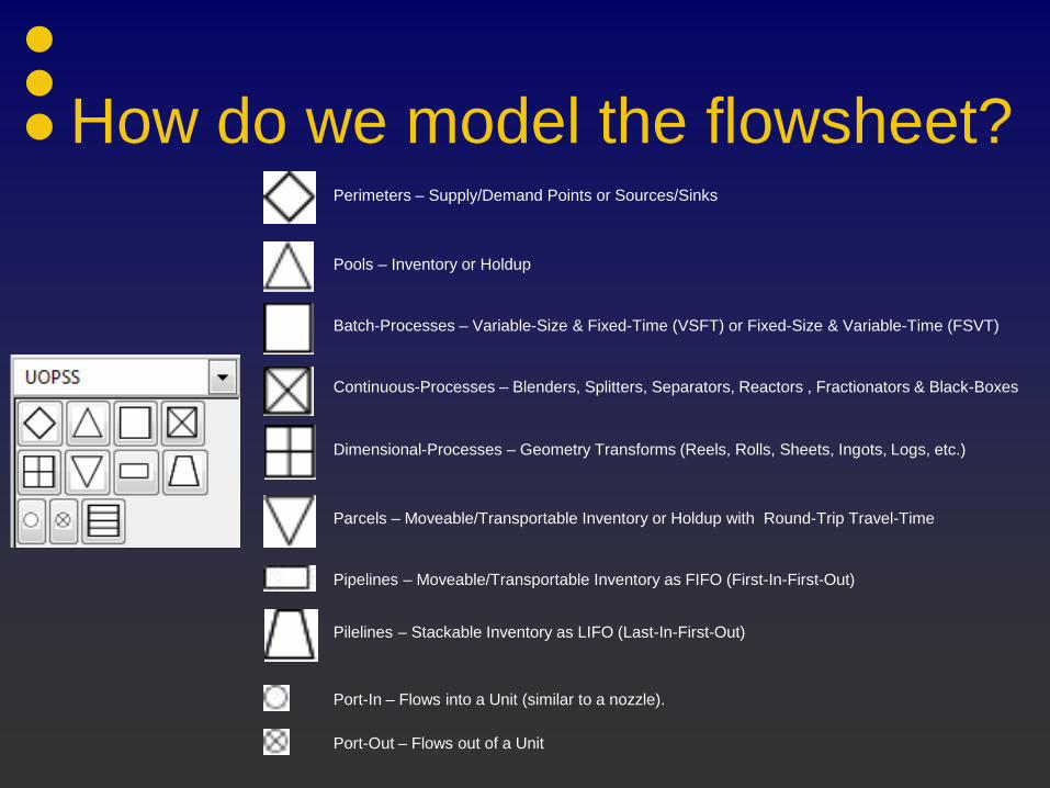
How do we model the flowsheet? Perimeters – Supply/Demand Points or Sources/Sinks

Pools – Inventory or Holdup

Batch-Processes – Variable-Size & Fixed-Time (VSFT) or Fixed-Size & Variable-Time (FSVT)

Continuous-Processes – Blenders, Splitters, Separators, Reactors , Fractionators & Black-Boxes

Parcels – Moveable/Transportable Inventory or Holdup with Round-Trip Travel-Time

Pipelines – Moveable/Transportable Inventory as FIFO (First-In-First-Out)

Port-In – Flows into a Unit (similar to a nozzle).

Port-Out – Flows out of a Unit

Dimensional-Processes – Geometry Transforms (Reels, Rolls, Sheets, Ingots, Logs, etc.)

Pilelines – Stackable Inventory as LIFO (Last-In-First-Out)

• IMPRESS has six system components we call SIIMPLE:– Server, Interfacer (IML), Interacter (IPL),

Modeler, Presolver DLL’s and an Executable (the executable can be coded in most computer programming language) .

– Interfacer, Interacter and Modeler are domain-specific whereas the Server, Presolver and Executable are not i.e., they are domain-inspecific or generic for any type of optimization problem.

What is our system architecture?

Jet Fuel Supply-Chain IMFNote: This flowsheet diagram was generated using GNOME Dia 0.97.2 and Python 2.3.5 with a custom UOPSS stencil.

Oil-Refinery Site• Three crude-oils of varying compositions.• A CDU (fractionator) with 8 compounds

(macro-cuts) with a charge of 20 Km3/day +/- 5% and 2 swing-cuts with 2 blenders.

• A VDU (fractionator) with 3 compounds and a possible import of reduced crude-oil.

• Jet Fuels A and B are blended with sulfur specifications of 0.125 & 0.250 wt%.

• Two dedicated tanks for Jet Fuel A and B of size 16 Km3 each. 15

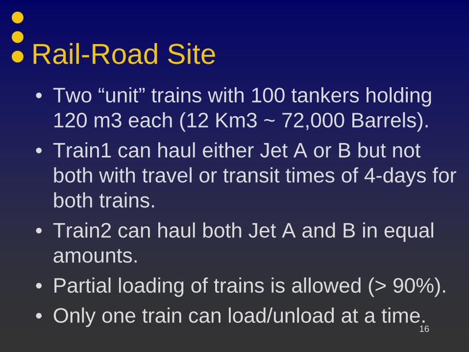
Rail-Road Site• Two “unit” trains with 100 tankers holding

120 m3 each (12 Km3 ~ 72,000 Barrels).• Train1 can haul either Jet A or B but not

both with travel or transit times of 4-days for both trains.

• Train2 can haul both Jet A and B in equal amounts.

• Partial loading of trains is allowed (> 90%).• Only one train can load/unload at a time.

16

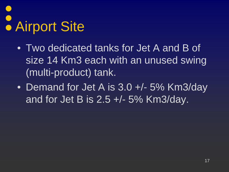
Airport Site• Two dedicated tanks for Jet A and B of

size 14 Km3 each with an unused swing (multi-product) tank.

• Demand for Jet A is 3.0 +/- 5% Km3/day and for Jet B is 2.5 +/- 5% Km3/day.

17

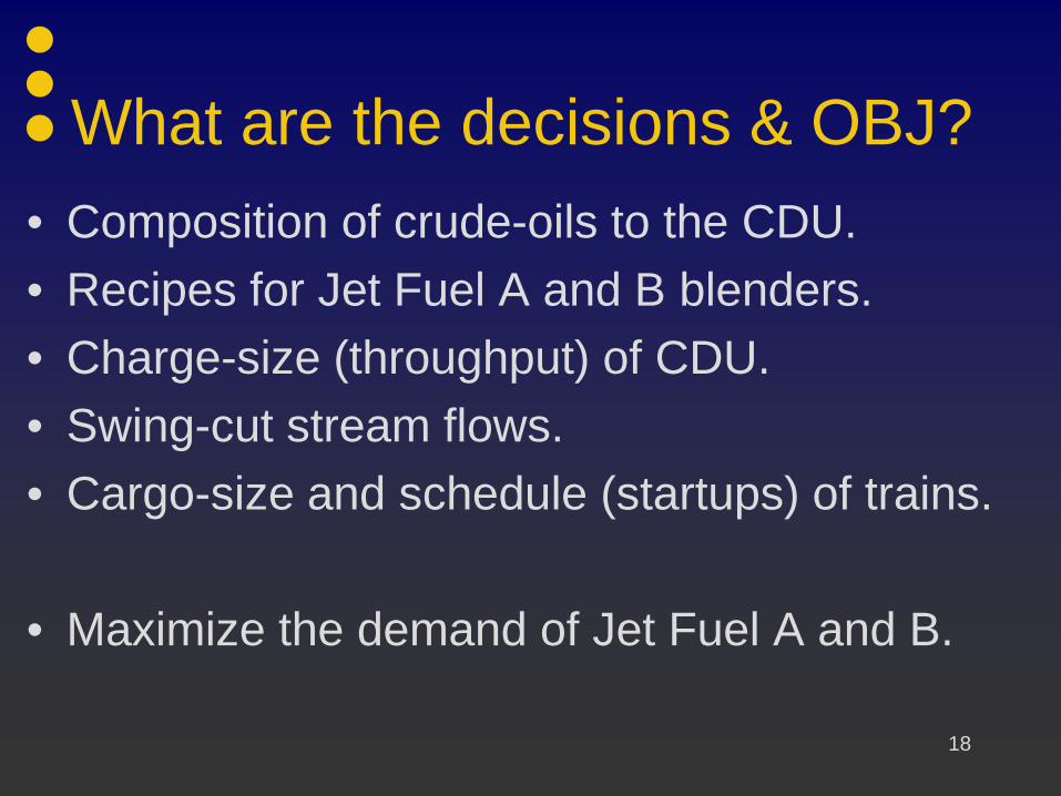
What are the decisions & OBJ?• Composition of crude-oils to the CDU.• Recipes for Jet Fuel A and B blenders.• Charge-size (throughput) of CDU.• Swing-cut stream flows. • Cargo-size and schedule (startups) of trains.

• Maximize the demand of Jet Fuel A and B.

18

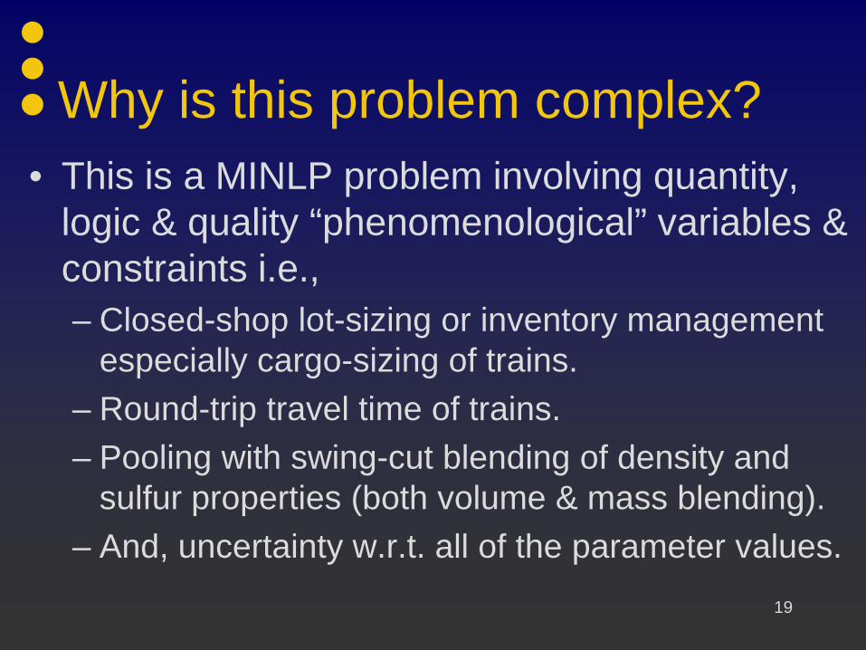
Why is this problem complex? • This is a MINLP problem involving quantity,

logic & quality “phenomenological” variables & constraints i.e.,– Closed-shop lot-sizing or inventory management

especially cargo-sizing of trains.– Round-trip travel time of trains.– Pooling with swing-cut blending of density and

sulfur properties (both volume & mass blending).– And, uncertainty w.r.t. all of the parameter values.

19

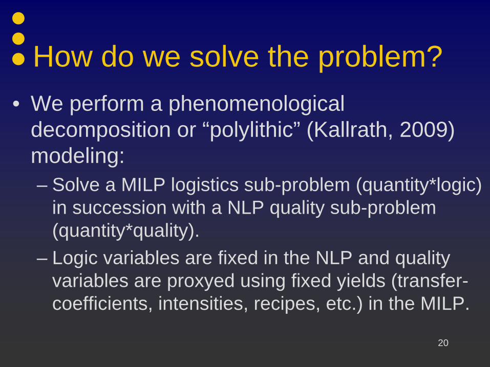
How do we solve the problem?• We perform a phenomenological

decomposition or “polylithic” (Kallrath, 2009) modeling:– Solve a MILP logistics sub-problem (quantity*logic)

in succession with a NLP quality sub-problem (quantity*quality).

– Logic variables are fixed in the NLP and quality variables are proxyed using fixed yields (transfer-coefficients, intensities, recipes, etc.) in the MILP.

20

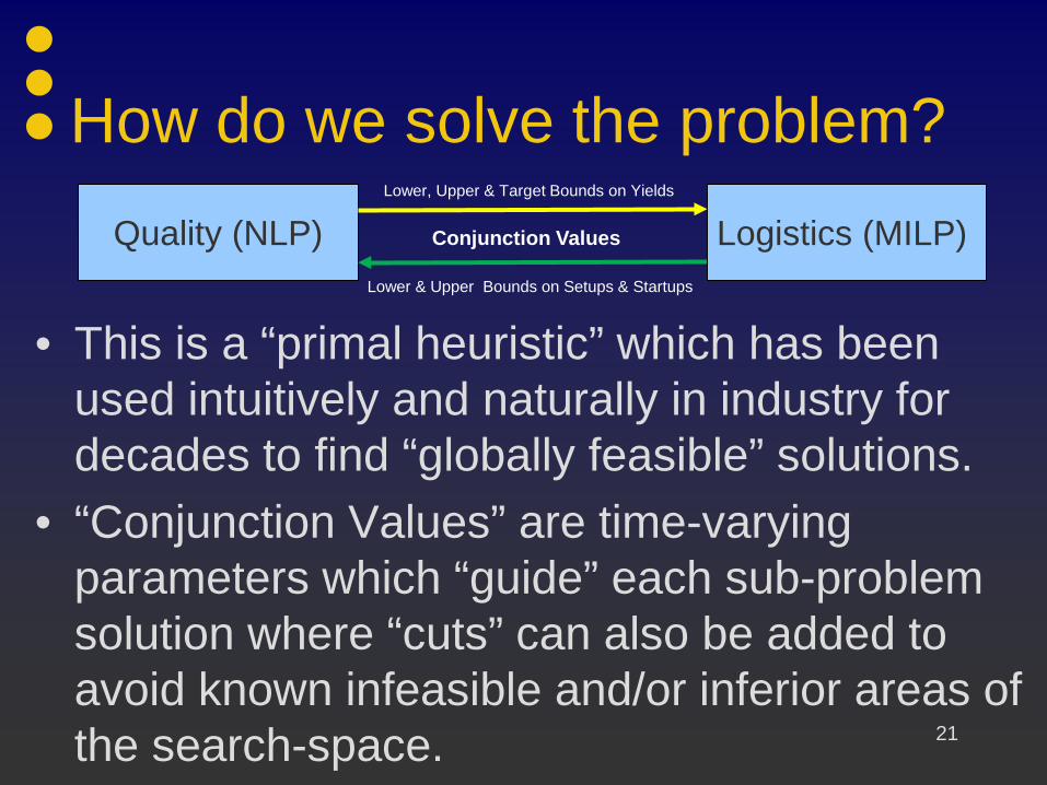
How do we solve the problem?Quality (NLP) Logistics (MILP)

Lower, Upper & Target Bounds on Yields

Lower & Upper Bounds on Setups & Startups

Conjunction Values

• This is a “primal heuristic” which has been used intuitively and naturally in industry for decades to find “globally feasible” solutions.

• “Conjunction Values” are time-varying parameters which “guide” each sub-problem solution where “cuts” can also be added to avoid known infeasible and/or inferior areas of the search-space. 21

What 3rd party solvers do we use?• For MILP we have bindings to:

– COINMP, GLPK, LPSOLVE, SCIP, CPLEX, GUROBI, LINDO & XPRESS.

• For NLP we have bindings to:– CONOPT, IPOPT, KNITRO, XPRESS-SLP as well

as our “home-grown” SLPQPE.– SLPQPE can use all previously mentioned LP’s as

its sub-solver. If the objective function has quadratic terms then a QP is called at each major iteration (for nonlinear control, data reconciliation & parameter estimation problems). 22

How do we manipulate the data?• All lower, upper (hard) and target (soft)

bounds are time-varying (temporal) for all QLQP variables.– Data are entered in continuous-time or event-

based and digitized into time-periods.– Data for over-lapping time-periods are

accumulated i.e., added or summed together.– Data are provided for both past/present and

future time-horizons (enabling data reconciliation and parameter estimation using the same model with different data). 23

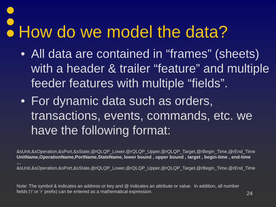
How do we model the data?• All data are contained in “frames” (sheets)

with a header & trailer “feature” and multiple feeder features with multiple “fields”.

• For dynamic data such as orders, transactions, events, commands, etc. we have the following format:

&sUnit,&sOperation,&sPort,&sState,@rQLQP_Lower,@rQLQP_Upper,@rQLQP_Target,@rBegin_Time,@rEnd_TimeUnitName,OperationName,PortName,StateName, lower bound , upper bound , target , begin-time , end-time…&sUnit,&sOperation,&sPort,&sState,@rQLQP_Lower,@rQLQP_Upper,@rQLQP_Target,@rBegin_Time,@rEnd_Time

Note: The symbol & indicates an address or key and @ indicates an attribute or value. In addition, all numberfields (‘i’ or ‘r’ prefix) can be entered as a mathematical expression. 24

How do we manage data for multiple sites (Hyperstructure)?

• Although not required for this small example, multiple “site” data is managed as follows:– Each site’s superstructure has its own separate IML

file included in a “hyperstructure” IML file.– Each site must have a unique name and all unit

names within the site are prefixed by this site name to make the site-unit pair namespace unique within the overall or multi-site model.

– Interchanges, interactions, interconnections, interplay, etc. between two or more sites is configured explicitly in the multi-site IML file. 25

Scenario Generation (Reactive)• We explore three types of ad hoc scenarios:

– Demand Variability– Tank Availability– Train Reliability

• One “base-case” IML file required with 3 “delta-case” incremental IML files for each scenario which “over-loads” the parameters.

• Goal of each delta-case scenario is to maintain “global feasibility” of logistics sub-problem given disturbance/disruption. 26

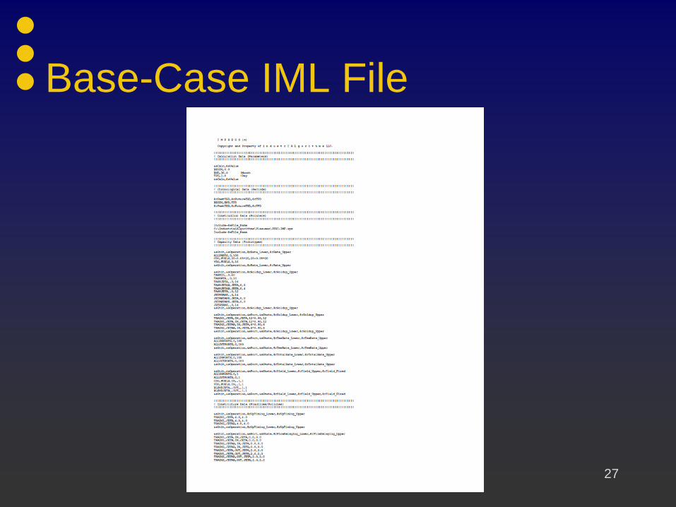
Base-Case IML File

27

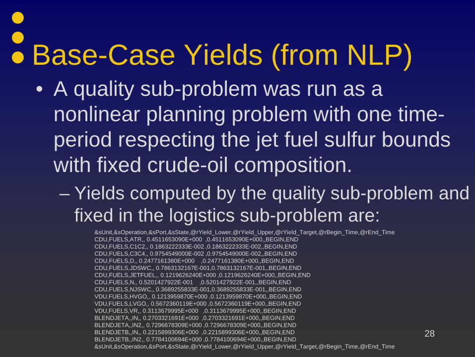
Base-Case Yields (from NLP)• A quality sub-problem was run as a

nonlinear planning problem with one time-period respecting the jet fuel sulfur bounds with fixed crude-oil composition.– Yields computed by the quality sub-problem and

fixed in the logistics sub-problem are:&sUnit,&sOperation,&sPort,&sState,@rYield_Lower,@rYield_Upper,@rYield_Target,@rBegin_Time,@rEnd_TimeCDU,FUELS,ATR,, 0.4511653090E+000 ,0.4511653090E+000,,BEGIN,ENDCDU,FUELS,C1C2,, 0.1863222333E-002 ,0.1863222333E-002,,BEGIN,ENDCDU,FUELS,C3C4,, 0.9754549000E-002 ,0.9754549000E-002,,BEGIN,ENDCDU,FUELS,D,, 0.2477161380E+000 ,0.2477161380E+000,,BEGIN,ENDCDU,FUELS,JDSWC,, 0.7863132167E-001,0.7863132167E-001,,BEGIN,ENDCDU,FUELS,JETFUEL,, 0.1219626240E+000 ,0.1219626240E+000,,BEGIN,ENDCDU,FUELS,N,, 0.5201427922E-001 ,0.5201427922E-001,,BEGIN,ENDCDU,FUELS,NJSWC,, 0.3689255833E-001,0.3689255833E-001,,BEGIN,ENDVDU,FUELS,HVGO,, 0.1213959870E+000 ,0.1213959870E+000,,BEGIN,ENDVDU,FUELS,LVGO,, 0.5672360119E+000 ,0.5672360119E+000,,BEGIN,ENDVDU,FUELS,VR,, 0.3113679995E+000 ,0.3113679995E+000,,BEGIN,ENDBLENDJETA,,IN,, 0.2703321691E+000 ,0.2703321691E+000,,BEGIN,ENDBLENDJETA,,IN2,, 0.7296678309E+000 ,0.7296678309E+000,,BEGIN,ENDBLENDJETB,,IN,, 0.2215899306E+000 ,0.2215899306E+000,,BEGIN,ENDBLENDJETB,,IN2,, 0.7784100694E+000 ,0.7784100694E+000,,BEGIN,END&sUnit,&sOperation,&sPort,&sState,@rYield_Lower,@rYield_Upper,@rYield_Target,@rBegin_Time,@rEnd_Time

28

Base-Case Statistics• Using thirty 1-day time-periods, the MILP has

circa 2225 variables, 3100 constraints, 10500 non-zeros and 750 binaries

• The objective function (OBJ) is $169.2 by arbitrarily maximizing the demand flow of Jet A and B equally i.e., prices = $1 per Km3.

• Using SCIP as the MILP solver, this takes 27-seconds.

29

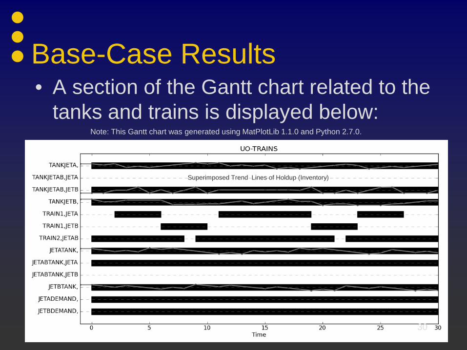
Base-Case Results• A section of the Gantt chart related to the

tanks and trains is displayed below:

Superimposed Trend Lines of Holdup (Inventory)

Note: This Gantt chart was generated using MatPlotLib 1.1.0 and Python 2.7.0.

30

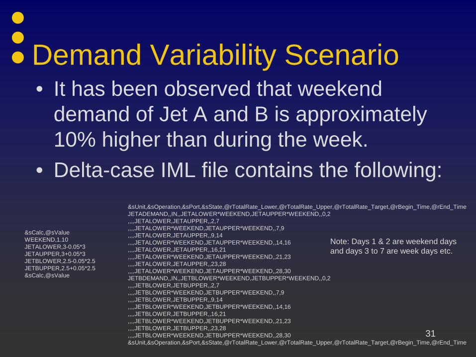
Demand Variability Scenario• It has been observed that weekend

demand of Jet A and B is approximately 10% higher than during the week.

• Delta-case IML file contains the following:

&sCalc,@sValueWEEKEND,1.10JETALOWER,3-0.05*3JETAUPPER,3+0.05*3JETBLOWER,2.5-0.05*2.5JETBUPPER,2.5+0.05*2.5&sCalc,@sValue

&sUnit,&sOperation,&sPort,&sState,@rTotalRate_Lower,@rTotalRate_Upper,@rTotalRate_Target,@rBegin_Time,@rEnd_TimeJETADEMAND,,IN,,JETALOWER*WEEKEND,JETAUPPER*WEEKEND,,0,2,,,,JETALOWER,JETAUPPER,,2,7,,,,JETALOWER*WEEKEND,JETAUPPER*WEEKEND,,7,9,,,,JETALOWER,JETAUPPER,,9,14,,,,JETALOWER*WEEKEND,JETAUPPER*WEEKEND,,14,16,,,,JETALOWER,JETAUPPER,,16,21,,,,JETALOWER*WEEKEND,JETAUPPER*WEEKEND,,21,23,,,,JETALOWER,JETAUPPER,,23,28,,,,JETALOWER*WEEKEND,JETAUPPER*WEEKEND,,28,30JETBDEMAND,,IN,,JETBLOWER*WEEKEND,JETBUPPER*WEEKEND,,0,2,,,,JETBLOWER,JETBUPPER,,2,7,,,,JETBLOWER*WEEKEND,JETBUPPER*WEEKEND,,7,9,,,,JETBLOWER,JETBUPPER,,9,14,,,,JETBLOWER*WEEKEND,JETBUPPER*WEEKEND,,14,16,,,,JETBLOWER,JETBUPPER,,16,21,,,,JETBLOWER*WEEKEND,JETBUPPER*WEEKEND,,21,23,,,,JETBLOWER,JETBUPPER,,23,28,,,,JETBLOWER*WEEKEND,JETBUPPER*WEEKEND,,28,30&sUnit,&sOperation,&sPort,&sState,@rTotalRate_Lower,@rTotalRate_Upper,@rTotalRate_Target,@rBegin_Time,@rEnd_Time

Note: Days 1 & 2 are weekend daysand days 3 to 7 are week days etc.

31

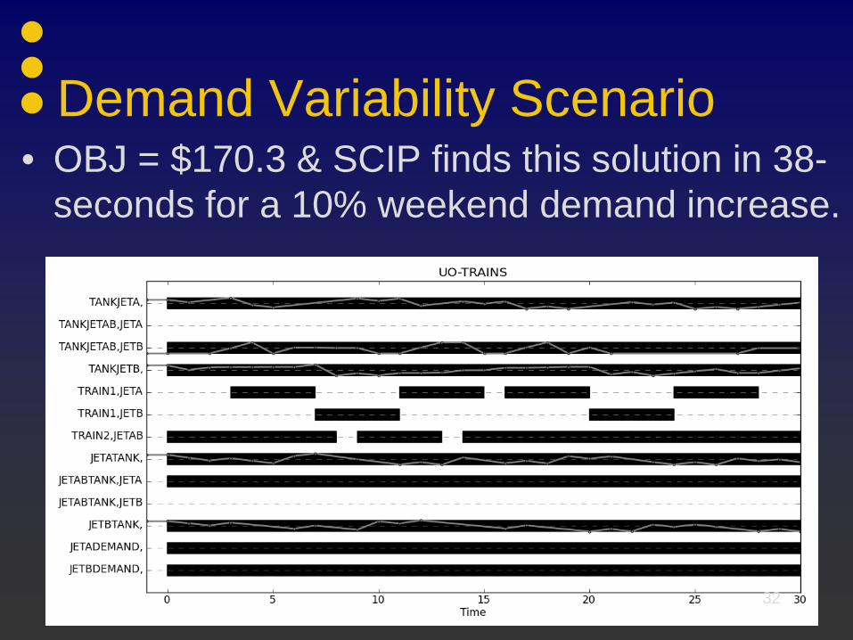
Demand Variability Scenario• OBJ = $170.3 & SCIP finds this solution in 38-

seconds for a 10% weekend demand increase.

32

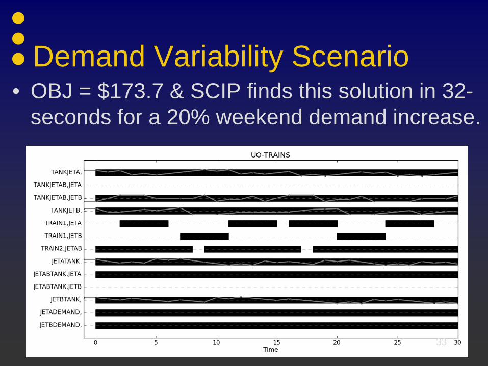
Demand Variability Scenario• OBJ = $173.7 & SCIP finds this solution in 32-

seconds for a 20% weekend demand increase.

33

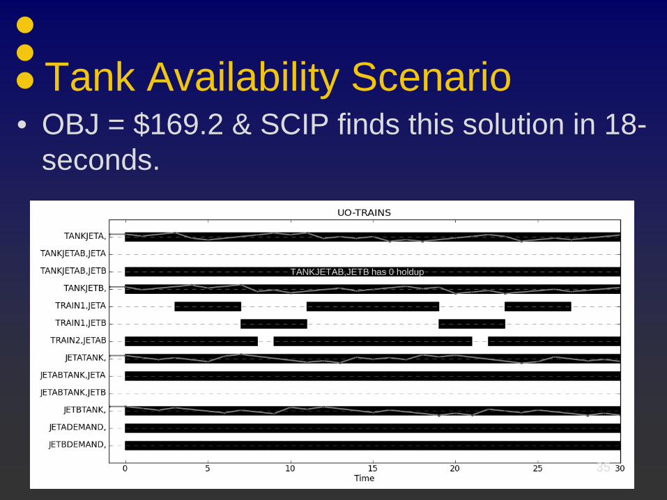
Tank Availability Scenario• Jet B demand is lower than Jet A and the

refinery has a smaller 12 Km3 tank that it would like to swap with the 16 Km3 Jet B tank and use it for gasoline production.

• Delta-case IML file contains the following:

&sUnit,&sOperation,@rHoldup_Lower,@rHoldup_UpperTANKJETA,,0,16TANKJETAB,JETA,0,0TANKJETAB,JETB,0,0TANKJETB,,0,12&sUnit,&sOperation,@rHoldup_Lower,@rHoldup_Upper

&sUnit,&sOperation,@rSetup_Lower,@rSetup_Upper,@rBegin_Time,@rEnd_TimeTANKJETAB,JETB,1,0,BEGIN,END&sUnit,&sOperation,@rSetup_Lower,@rSetup_Upper,@rBegin_Time,@rEnd_Time

34

Tank Availability Scenario

TANKJETAB,JETB has 0 holdup

• OBJ = $169.2 & SCIP finds this solution in 18-seconds.

35

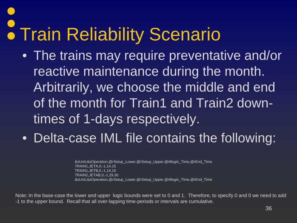
Train Reliability Scenario• The trains may require preventative and/or

reactive maintenance during the month. Arbitrarily, we choose the middle and end of the month for Train1 and Train2 down-times of 1-days respectively.

• Delta-case IML file contains the following:&sUnit,&sOperation,@rSetup_Lower,@rSetup_Upper,@rBegin_Time,@rEnd_TimeTRAIN1,JETA,0,-1,14,15TRAIN1,JETB,0,-1,14,15TRAIN2,JETAB,0,-1,29,30 &sUnit,&sOperation,@rSetup_Lower,@rSetup_Upper,@rBegin_Time,@rEnd_Time

Note: In the base-case the lower and upper logic bounds were set to 0 and 1. Therefore, to specify 0 and 0 we need to add-1 to the upper bound. Recall that all over-lapping time-periods or intervals are cumulative.

36

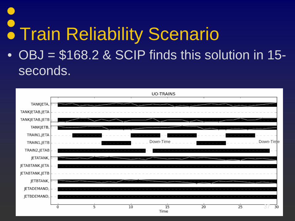
Train Reliability Scenario

Down-Time Down-Time

• OBJ = $168.2 & SCIP finds this solution in 15-seconds.

37

How do we compare solutions of multiple scenarios?• By defining aggregations or key performance

indicators (KPI’s) and computing them in a computer programming language (Python).

• By displaying multiple solutions in the same Gantt chart, trend plot, etc. i.e., OLAP, IBM’s ILOG ODM or FICO’s Xpress-Insights.

• By data-mining the solutions using compressing & clustering techniques such as PCA, PLS, K-Means Centering, Fuzzy-C-Mean Clustering, etc. 38

Acknowledgements• We would especially like to thank Prof.

Grossmann for providing us this opportunity to present to the EWO members.

39

Questions

• Thank You!

40