Survey of NLP Algorithms

L. T. BieglerChemical Engineering Department

Carnegie Mellon UniversityPittsburgh, PA

2

NLP Algorithms - Outline

•Problem and Goals

•KKT Conditions and Variable Classification

•Handling Basic Variables

•Handling Nonbasic Variables

•Handling Superbasic Variables

•Ensuring Global Convergence

•Algorithms and Software

•Algorithmic Comparison

•Summary and Future Work

3

Problem: Minx f(x)s.t. g(x) ≤ 0

h(x) = 0where:

f(x) - scalar objective functionx - n vector of variables

g(x) - inequality constraints, m vectorh(x) - meq equality constraints.

Sufficient Condition for Unique Optimum- f(x) must be convex, and- feasible region must be convex,

i.e. g(x) are all convexh(x) are all linear

Except in special cases, there is no guarantee that a local optimum is globalif sufficient conditions are violated.

Constrained Optimization(Nonlinear Programming)

4

Min f(x) Min f(z)s.t. g(x) + s = 0 (add slack variable) ⇒ s.t. c(z) = 0

h(x) = 0, s ≥ 0 a ≤ z ≤ b

• Partition variables into: zB - dependent or basic variableszN - nonbasic variables, fixed at a boundzS - independent or superbasic variables

Analogy to linear programming. Superbasics required only if nonlinear problem

Variable Classification for NLPs

5

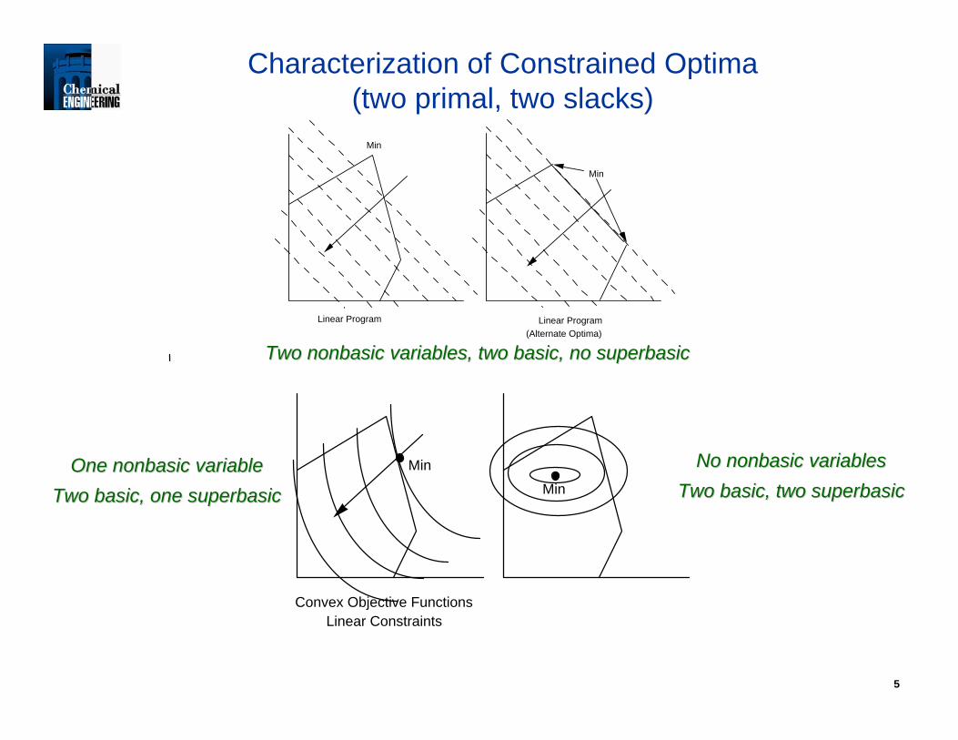
Min

Linear Program

Min

Linear Program(Alternate Optima)

Characterization of Constrained Optima(two primal, two slacks)

Two Two nonbasicnonbasic variables, two basic, no variables, two basic, no superbasicsuperbasic

Min

Min

Min

Convex Objective FunctionsLinear Constraints

One One nonbasicnonbasic variablevariableTwo basic, one Two basic, one superbasicsuperbasic

No No nonbasicnonbasic variablesvariablesTwo basic, two Two basic, two superbasicsuperbasic

6

What conditions characterize an optimal solution?

Unconstrained Local MinimumNecessary Conditions

∇f (x*) = 0pT∇2f (x*) p ≥ 0 for p∈ℜn

(positive semi-definite)

Unconstrained Local MinimumSufficient Conditions

∇f (x*) = 0pT∇2f (x*) p > 0 for p∈ℜn

(positive definite)

7

Optimal solution for inequality constrained problem

Min f(x)s.t . g(x) ≤ 0

Analogy: Ball rolling down valley pinned by fenceNote: Balance of forces (∇f, ∇g1)

8

Optimal solution for general constrained problem

Problem: Min f(x)s.t. g(x) ≤ 0

h(x) = 0Analogy: Ball rolling on rail pinned by fencesBalance of forces: ∇f, ∇g1, ∇h

9

Necessary First Order Karush Kuhn - Tucker Conditions

∇ L (z*, u, v) = ∇f(x*) + ∇g(x*) u + ∇h(x*) v = 0 (Balance Forces)u ≥ 0 (Inequalities act in only one direction)g (x*) ≤ 0, h (x*) = 0 (Feasibility)uj gj(x*) = 0 (Complementarity: either gj(x*) = 0 or uj = 0)u, v are "weights" for "forces," known as KKT multipliers, shadow prices, dual variables

“To guarantee that a local NLP solution satisfies KKT conditions, a constraint qualification is required. E.g., the Linear Independence Constraint Qualification(LICQ) requires active constraint gradients, [∇gA(x*) ∇h(x*)], to be linearlyindependent. Also, under LICQ, KKT multipliers are uniquely determined.”

Necessary (Sufficient) Second Order Conditions- Positive curvature in "constraint" directions.- pT∇ 2L (x*) p ≥ 0 (pT∇ 2L (x*) p > 0)

where p are the constrained directions: ∇gA(x*)Tp = 0, ∇h(x*)Tp = 0This is the space of the superbasic variables!

Optimality conditions for local optimum

10

Min f(z), s.t. c(z) = 0, a ≤ z ≤ b

∇ L (z*, λ, ν) = ∇f(z*) + ∇c(z*) λ - νa + νb = 0 (Balance Forces)a ≤ z* ≤ b, c (z*) = 0 (Feasibility)

0 ≤ z*- a perp νa ≥ 00 ≤ b - z* perp νb ≥ 0

In terms of partitioned variables (when known)Basic (nb = m): ∇ ΒL (z*, λ, ν) = ∇ Β f(z*) + ∇ Β c(z*) λ = 0

c (z*) = 0Square system in zB and λ

Nonbasic (nn): ∇ Ν L (z*, λ, ν) = ∇ Ν f(z*) + ∇ Ν c(z*) λ – νbnd = 0z*= bnd

Square system in zN and ν

Superbasic (ns): ∇ SL (z*, λ, ν) = ∇ S f(z*) + ∇ S c(z*) λ = 0Square system in zS

n = nn+ nb + ns

Optimality conditions for local optimum

11

Handling Basic Variables

∇ ΒL (z*, λ, ν) = ∇ Β f(z*) + ∇ Β c(z*) λ = 0c (z*) = 0

Full space: linearization and simultaneous solution of c(z) = 0 with stationarityconditions.

– embedded within Newton method for KKT conditions (SQP and Barrier)

Reduced space (two flavors):

- elimination of nonlinear equations and zB at every point (feasible path GRG

methods)

- linearization, then elimination of linear equations and zB (MINOS and rSQP)

12

Handling Nonbasic Variables

∇ Ν L (z*, λ, ν) = ∇ Ν f(z*) + ∇ Ν c(z*) λ – νbnd = 0z*= bnd

Barrier approach - primal and primal-dual approaches (IPOPT, KNITRO, LOQO)

Active set (two flavors)• QP or LP subproblems - primal-dual pivoting (SQP)• gradient projection in primal space with bound constraints (GRG)

13

Gradient Projection Method(nonbasic variable treatment)

Define the projection of an arbitrary point x onto box feasible region.

The ith component is given by

Piecewise linear path x(t) starting at the reference point x0 and obtained by projecting steepest descent direction at x0 onto the box region is given by

14

Handling Superbasic Variables

∇ SL (z*, λ, ν) = ∇ S f(z*) + ∇ S c(z*) λ = 0

Second derivatives or quasi-Newton?

BFGS Formula s = xk+1 - xk

y = ∇L(xk+1, uk+1, vk+1) - ∇L(xk, uk+1, vk+1)• second derivatives approximated by change in gradients• positive definite Bk ensures unique search direction and descent property

Exact Hessian – requires far fewer iterations (no buildup needed in space of superbasics)

full-space - exploit sparsity (efficient large-scale solvers needed)reduced space - update or project (expensive dense algebra if ns large)

k+1B = kB + Tyy

Ts y -

kB s Ts kBks B s

15

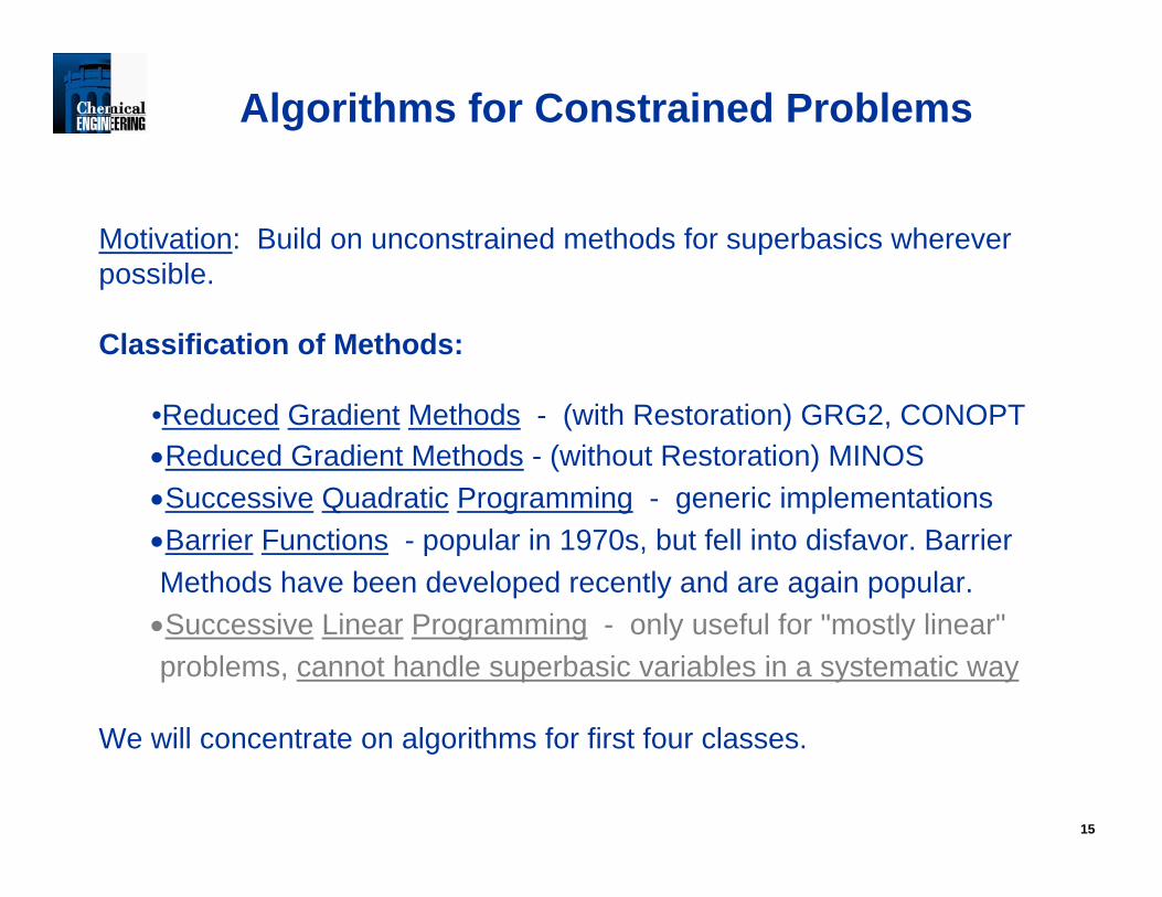
Motivation: Build on unconstrained methods for superbasics wherever possible.

Classification of Methods:

•Reduced Gradient Methods - (with Restoration) GRG2, CONOPT •Reduced Gradient Methods - (without Restoration) MINOS•Successive Quadratic Programming - generic implementations•Barrier Functions - popular in 1970s, but fell into disfavor. Barrier Methods have been developed recently and are again popular.

•Successive Linear Programming - only useful for "mostly linear" problems, cannot handle superbasic variables in a systematic way

We will concentrate on algorithms for first four classes.

Algorithms for Constrained Problems

16

•Nonlinear elimination of basic variables (and multipliers, λ)•Use gradient projection to update and remove nonbasic variables•Solve problem in reduced space of superbasic variables using the concept of reduced gradients

Reduced Gradient Methods

[ ]

[ ]B

zzSS

zzBSS

B

B

T

BS

T

S

BS

B

SS

zfcc

zf

dzdf

cczc

zc

dzdz

dzzcdz

zcdc

,)z(czf

dzdz

zf

dzdf

BS

BS

∂∂

∇∇−∂∂

=

∇−∇=⎥⎦

⎤⎢⎣

⎡∂∂

⎥⎦

⎤⎢⎣

⎡∂∂

−=

=⎥⎦

⎤⎢⎣

⎡∂∂

+⎥⎦

⎤⎢⎣

⎡∂∂

=

=∂∂

+∂∂

=

−

−−

1

11

:superbasicfor gradient reduced toleads This

0

:have we0 Because

17

If ∇cT is (m x n); ∇zScT is m x (n-m); ∇zBcT is (m x m)

(df/dzS) is the change in f along constraint direction per unit change in zS

Example of Reduced Gradient

[ ]

[ ] ( ) 2/322-432

Let

2]- 2[ 4], 3[

2443 ..2

11

11

1

21

1

21

22

1

+=−=

∂∂

∇∇−∂∂

=

==

=∇=∇

=+−

−

−

xxdxdf

zfcc

zf

dzdf

x, zxz

xfc

xxtsxxMin

Bzz

SS

BS

TT

BS

18

Sketch of GRG Algorithm1.1. Initialize problem and obtain a feasible point at zInitialize problem and obtain a feasible point at z00

2.2. At feasible point At feasible point zzkk, partition variables , partition variables zz into into zzNN, , zzBB, , zzSS

3.3. Remove Remove nonbasicsnonbasics4.4. Calculate reduced gradient, Calculate reduced gradient, ((df/dzdf/dzSS))5.5. Evaluate search direction for Evaluate search direction for zzSS, , d = Bd = B--11(df/dz(df/dzSS) ) 6.6. Perform a line search.Perform a line search.

•• Find Find αα∈∈(0,1](0,1] withwith zzSS := := zzSSkk + + αα dd

•• Solve for Solve for c(zc(zSSkk + + αα d, d, zzBB, , zzNN) = 0) = 0

•• If If f(zf(zSSkk + + αα dd, , zzBB, , zzNN) ) < < f(zf(zSS

kk, , zzBB, , zzNN), ), setset zzSS

k+1 k+1 ==zzSSkk + + αα d, k:= k+1d, k:= k+1

7.7. If ||If ||((df/dzdf/dzSS)||<)||<ε, ε, Stop. Else, go to 2. Stop. Else, go to 2.

19

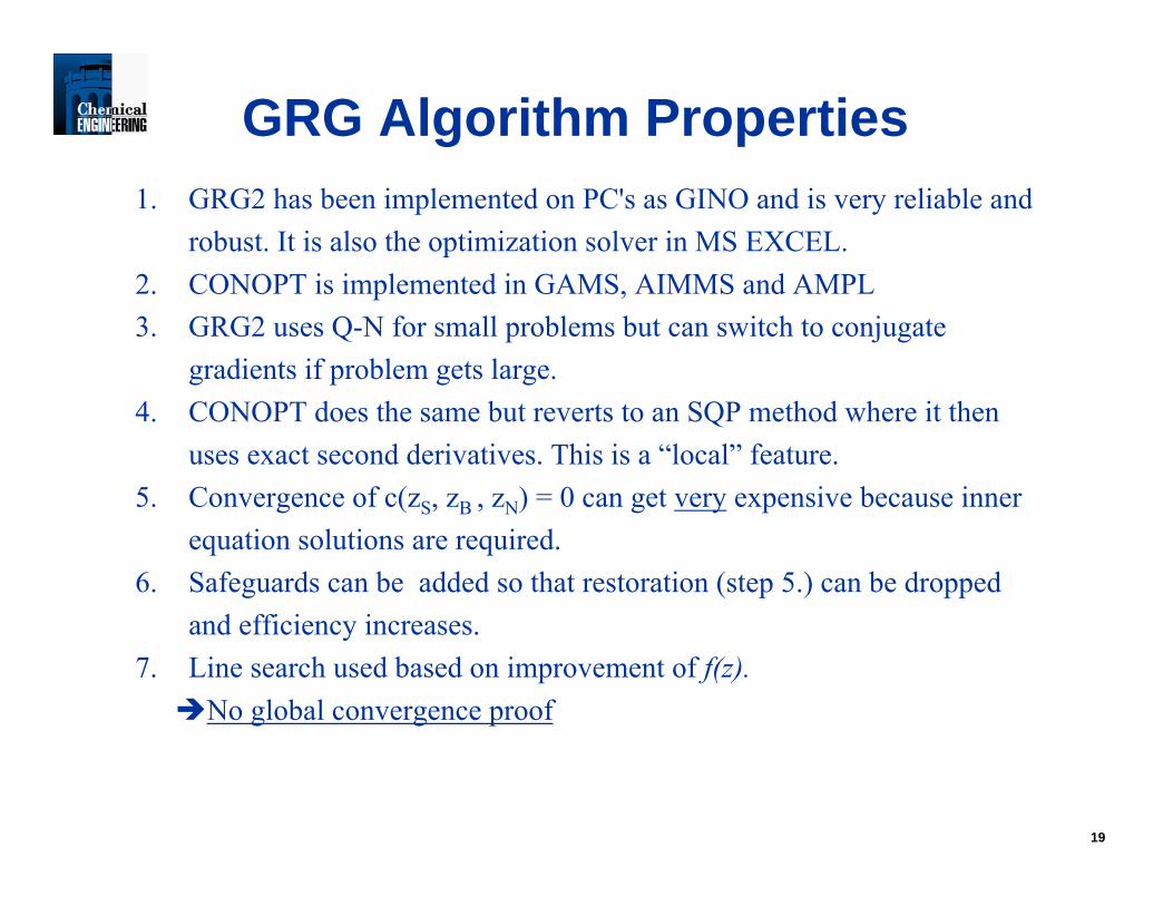
1. GRG2 has been implemented on PC's as GINO and is very reliable and robust. It is also the optimization solver in MS EXCEL.

2. CONOPT is implemented in GAMS, AIMMS and AMPL3. GRG2 uses Q-N for small problems but can switch to conjugate

gradients if problem gets large. 4. CONOPT does the same but reverts to an SQP method where it then

uses exact second derivatives. This is a “local” feature.5. Convergence of c(zS, zB , zN) = 0 can get very expensive because inner

equation solutions are required. 6. Safeguards can be added so that restoration (step 5.) can be dropped

and efficiency increases.7. Line search used based on improvement of f(z).

No global convergence proof

GRG Algorithm Properties

20

Motivation: Efficient algorithms are available that solve linearly constrained optimization problems (MINOS):

Min f(x)s.t. Ax ≤ b

Cx = d

Extend to nonlinear problems, through successive linearization

Develop major iterations (linearizations) and minor iterations (GRG solutions) .

Reduced Gradient Method without Restoration“Linearize then Eliminate Basics”

(MINOS/Augmented)

Strategy: (Robinson, Murtagh & Saunders)1. Partition variables into basic, nonbasic

variables and superbasic variables.. 2. Linearize active constraints at zk

Dkz = rk

3. Let ψ = f (z) + vTc (z) + β (c(z)Tc(z))(Augmented Lagrange),

4. Solve linearly constrained problem:Min ψ (z)s.t. Dz = r

a ≤ z ≤ busing reduced gradients to get zk+1

5. Set k=k+1, go to 3.6. Algorithm terminates when no

movement between steps 3) and 4).

21

1. MINOS has been implemented very efficiently to take care of linearity. It becomes LP Simplex method if problem is totally linear. Also, very efficient matrix routines.

2. No restoration takes place, nonlinear constraints are reflected in ψ(z) during step 3). MINOS is more efficient than GRG.

3. Major iterations (steps 3) - 4)) converge at a quadratic rate.4. Reduced gradient methods are complicated, monolithic codes:

hard to integrate efficiently into modeling software.5. No globalization and no global convergence proof

MINOS/Augmented Notes

22

Motivation:• Take KKT conditions, expand in Taylor series about current point.• Take Newton step (QP) to determine next point.

Derivation – KKT Conditions∇xL (x*, u*, v*) = ∇f(x*) + ∇gA(x*) u* + ∇h(x*) v* = 0

h(x*) = 0 gA(x*) = 0, where gA are the active constraints.

Newton - Step

xx∇ LAg∇ ∇ h

Ag∇ T 0 0

∇ hT 0 0

⎡

⎣

⎢ ⎢ ⎢ ⎢

⎤

⎦

⎥ ⎥ ⎥ ⎥

ΔxΔuΔv

⎡

⎣

⎢ ⎢ ⎢

⎤

⎦

⎥ ⎥ ⎥

= -

x∇ L kx , ku , kv( )Ag kx( )h kx( )

⎡

⎣

⎢ ⎢ ⎢ ⎢

⎤

⎦

⎥ ⎥ ⎥ ⎥

Requirements:• ∇xxL must be calculated and should be ‘regular’•correct active set gA, need to know nonbasic variables!•good estimates of uk, vk

Successive Quadratic Programming (SQP)

23

1. Wilson (1963)- active set (nonbasics) can be determined by solving QP:

Min ∇f(xk)Td + 1/2 dT ∇xx L(xk, uk, vk) dd

s.t. g(xk) + ∇g(xk)T d ≤ 0h(xk) + ∇h(xk)T d = 0

2. Han (1976), (1977), Powell (1977), (1978)- approximate ∇xxL using a positive definite quasi-Newton update (BFGS)- use a line search to converge from poor starting points.

Notes:- Similar methods were derived using penalty (not Lagrange) functions.- Method converges quickly; very few function evaluations.- Not well suited to large problems (full space update used).

For n > 100, say, use reduced space methods (e.g. MINOS).

SQP Chronology

24

How do we obtain search directions?• Form QP and let QP determine constraint activity• At each iteration, k, solve:

Min ∇f(xk) Td + 1/2 dT Bkdd

s.t. g(xk) + ∇g(xk) T d ≤ 0h(xk) + ∇h(xk) T d = 0

Convergence from poor starting points• As with Newton's method, choose α (stepsize) to ensure progress

toward optimum: xk+1 = xk + α d.• α is chosen by making sure a merit function is decreased at each

iteration.Exact Penalty Functionψ(x) = f(x) + μ [Σ max (0, gj(x)) + Σ |hj (x)|]

μ > maxj {| uj |, | vj |}Augmented Lagrange Functionψ(x) = f(x) + uTg(x) + vTh(x)

+ η/2 {Σ (hj (x))2 + Σ max (0, gj (x))2}

Elements of SQP – Search Directions

25

Fast Local ConvergenceB = ∇xxL Quadratic∇xxL is p.d and B is Q-N 1 step SuperlinearB is Q-N update, ∇xxL not p.d 2 step Superlinear

Enforce Global ConvergenceEnsure decrease of merit function by taking α ≤ 1Trust region adaptations provide a stronger guarantee of global convergence - but harder to implement.

Newton-Like Properties for SQP

26

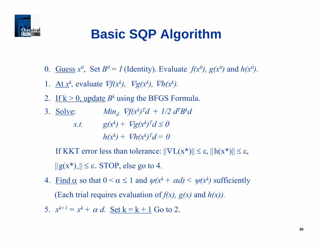
0. Guess x0, Set B0 = I (Identity). Evaluate f(x0), g(x0) and h(x0).

1. At xk, evaluate ∇f(xk), ∇g(xk), ∇h(xk).

2. If k > 0, update Bk using the BFGS Formula.3. Solve: Mind ∇f(xk)Td + 1/2 dTBkd

s.t. g(xk) + ∇g(xk)Td ≤ 0h(xk) + ∇h(xk)Td = 0

If KKT error less than tolerance: ||∇L(x*)|| ≤ ε, ||h(x*)|| ≤ ε,

||g(x*)+|| ≤ ε. STOP, else go to 4.

4. Find α so that 0 < α ≤ 1 and ψ(xk + αd) < ψ(xk) sufficiently

(Each trial requires evaluation of f(x), g(x) and h(x)).

5. xk+1 = xk + α d. Set k = k + 1 Go to 2.

Basic SQP Algorithm

27

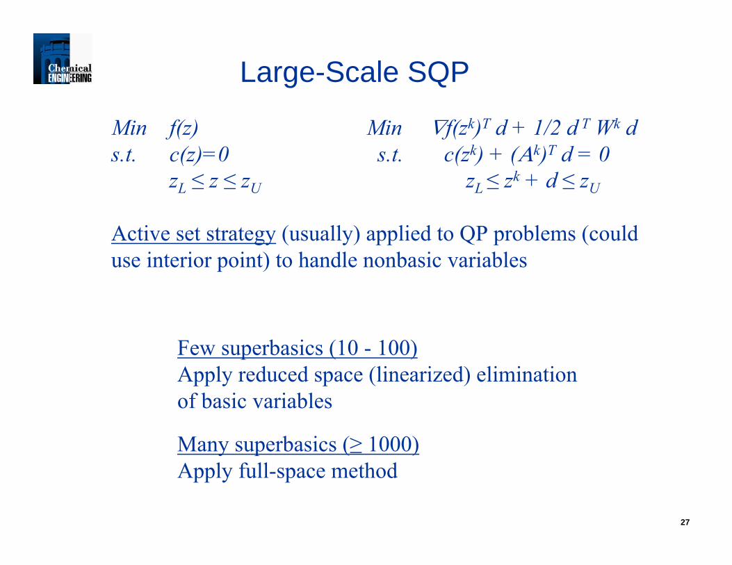
Min f(z) Min ∇f(zk)T d + 1/2 d T Wk ds.t. c(z)=0 s.t. c(zk) + (Αk)T d = 0

zL ≤ z ≤ zU zL ≤ zk + d ≤ zU

Active set strategy (usually) applied to QP problems (could use interior point) to handle nonbasic variables

Few superbasics (10 - 100)Apply reduced space (linearized) elimination of basic variables

Many superbasics (≥ 1000)Apply full-space method

Large-Scale SQP

28

• Take advantage of sparsity of A=∇c(x)• project W into space of active (or equality constraints)• curvature (second derivative) information only needed in space of degrees of

freedom• second derivatives can be applied or approximated with positive curvature

(e.g., BFGS)• use dual space QP solvers

+ easy to implement with existing sparse solvers, QP methods and line search techniques

+ exploits 'natural assignment' of dependent and decision variables (some decomposition steps are 'free')

+ does not require second derivatives

- reduced space matrices are dense- may be dependent on variable partitioning- can be very expensive for many degrees of freedom- can be expensive if many QP bounds

Few degrees of freedom => reduced space SQP (rSQP)

29

Reduced space SQP (rSQP)Range and Null Space Decomposition

⎥⎦

⎤⎢⎣

⎡∇−=⎥

⎦

⎤⎢⎣

⎡⎥⎦

⎤⎢⎣

⎡

+ )()(

0 k

k

Tk

kk

xcxfd

AAW

λ

Assume nonbasics removed, QP problem with n variables and mconstraints becomes:

• Define reduced space basis, Zk∈ ℜn x (n-m) with (Ak)TZk = 0• Define basis for remaining space Yk∈ ℜn x m, [Yk Zk]∈ℜn x n

is nonsingular. • Let d = Yk dY + Zk dZ to rewrite:

[ ] [ ] [ ]⎥⎦

⎤⎢⎣

⎡∇

⎥⎥⎦

⎤

⎢⎢⎣

⎡−=

⎥⎥

⎦

⎤

⎢⎢

⎣

⎡⎥⎦

⎤⎢⎣

⎡⎥⎦

⎤⎢⎣

⎡

⎥⎥⎦

⎤

⎢⎢⎣

⎡

+)()(

00

00

000

k

kTkk

Z

Ykk

Tk

kkTkk

xcxf

IZY

dd

IZY

AAW

IZY

λ

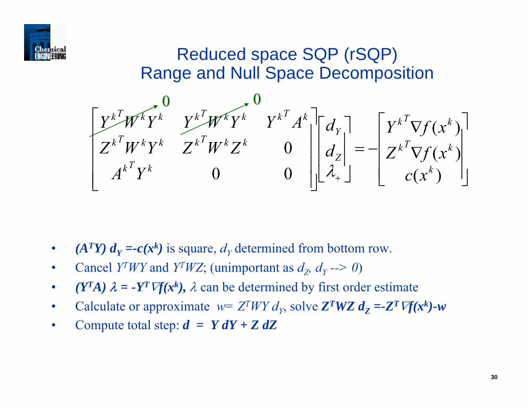
30

Reduced space SQP (rSQP)Range and Null Space Decomposition

• (ATY) dY =-c(xk) is square, dY determined from bottom row.• Cancel YTWY and YTWZ; (unimportant as dZ, dY --> 0)• (YTA) λ = -YT∇f(xk), λ can be determined by first order estimate• Calculate or approximate w= ZTWY dY, solve ZTWZ dZ =-ZT∇f(xk)-w• Compute total step: d = Y dY + Z dZ

⎥⎥⎥

⎦

⎤

⎢⎢⎢

⎣

⎡

∇∇

−=⎥⎥

⎦

⎤

⎢⎢

⎣

⎡

⎥⎥⎥⎥

⎦

⎤

⎢⎢⎢⎢

⎣

⎡

+ )()()(

000

k

kTk

kTk

Z

Y

kTk

kkTkkkTk

kTkkkTkkkTk

xcxfZxfY

dd

YAZWZYWZ

AYYWYYWY

λ

00 00

31

Barrier Methods for Large-Scale Nonlinear Programming

0 0)(s.t

)(min

≥=

ℜ∈

xxc

xfnx

Original Formulation

0)(s.t

ln)()( min1

=

−= ∑=ℜ∈

xc

xxfxn

ii

x nμϕμBarrier Approach

Can generalize for

bxa ≤≤

⇒As μ 0, x*(μ) x* Fiacco and McCormick (1968)

32

Solution of the Barrier Problem

⇒Newton Directions (KKT System)

0 )(0 0 )()(

==−=−+∇

xceXvvxAxf

μλ

⇒Solve

⎥⎥⎥

⎦

⎤

⎢⎢⎢

⎣

⎡

−

−+∇−=

⎥⎥⎥

⎦

⎤

⎢⎢⎢

⎣

⎡

⎥⎥⎥

⎦

⎤

⎢⎢⎢

⎣

⎡ −

eXvc

vAf

ddd

XVA

IAW x

000

μ

λ

ν

λ

⇒ Reducing the Systemxv VdXveXd 11 −− −−=μ

⎥⎦

⎤⎢⎣

⎡∇−=⎥

⎦

⎤⎢⎣

⎡⎥⎦

⎤⎢⎣

⎡ Σ++ c

dA

AW xT

μϕλ

0 VX 1−=Σ

IPOPT Code IPOPT Code –– www.coinwww.coin--or.orgor.org

)(...]1 ,1 ,1[xdiagX

eT

==

33

Global Convergence of Newton-based Barrier Solvers

Merit Function

Exact Penalty: P(x, η) = f(x) + η ||c(x)||

Aug’d Lagrangian: L*(x, λ, η) = f(x) + λTc(x) + η ||c(x)||2

Assess Search Direction (e.g., from IPOPT)

Line Search – choose stepsize α to give sufficient decrease of merit function using a ‘step to the boundary’ rule with τ ~0.99.

• How do we balance φ (x) and c(x) with η?• Is this approach globally convergent? Will it still be fast?

)( 0)1(

0)1( ],,0( for

1

1

1

kkk

kvkk

kxk

xkk

vdvvxdx

dxx

λλαλλτα

ταααα

−+=>−≥+=

>−≥++=∈

++

+

+

34

Line Search Filter Method

Store (φk, θk) at allowed iterates

Allow progress if trial point is acceptable to filter with θ margin

If switching condition

is satisfied, only an Armijo line search is required on φk

If insufficient progress on stepsize, evoke restoration phase to reduce θ.

Global convergence and superlinearlocal convergence proved (with second order correction)

22,][][ >>≥−∇ bad bk

aTk θδφα

φ(x)

θ(x) = ||c(x)||

35

IPOPT Algorithm – Features

Line Search Strategies for Globalization

- l2 exact penalty merit function

- Filter method (adapted and extended from Fletcher and Leyffer)

Hessian Calculation

- BFGS (full/LM)

- SR1 (full/LM)

- Exact full Hessian (direct)

- Exact reduced Hessian (direct)

- Preconditioned CG

Algorithmic PropertiesGlobally, superlinearlyconvergent (Wächter and B., 2005)

Easily tailored to different problem structures

Freely AvailableCPL License and COIN-OR distribution: http://www.coin-or.org

Beta version recently rewritten in C++

Solved on thousands of test problems and applications

36

⎥⎦

⎤⎢⎣

⎡−=⎥

⎦

⎤⎢⎣

⎡⎥⎦

⎤⎢⎣

⎡

k

k

k

Tkk

cgd

AAW

λ0

Trust Region Barrier Method Trust Region Barrier Method KNITROKNITRO

37

Composite Step Trust-region SQPSplit barrier problem step into 2 parts: normal (basic) and tangential

(nonbasic and superbasic) search directions

Trust-region on tangential component: larger combined radius

xk

dN

Zdθδ2

δ1

d

38

KNITRO Algorithm – Features

Overall method

- Similar to IPOPT

- But does not use filter method

- applies full-space Newton step and line search (LOQO is similar)

Trust Region Strategies for Globalization

- based on l2 exact penalty merit function

- expensive: used only when line search approach gets “into trouble”

Tangential Problem

- Exact full Hessian (direct)

- Preconditioned CG to solve tangential problem

Normal Problem

- use dogleg method based on Cauchy step

Algorithmic PropertiesGlobally, superlinearlyconvergent (Byrd and Nocedal, 2000)

Stronger convergence properties using trust region over line search

Available through ZeniaAvailable free to academicshttp://www.neos.mcs.anl.gov

Solved on thousands of test problems and applications

39

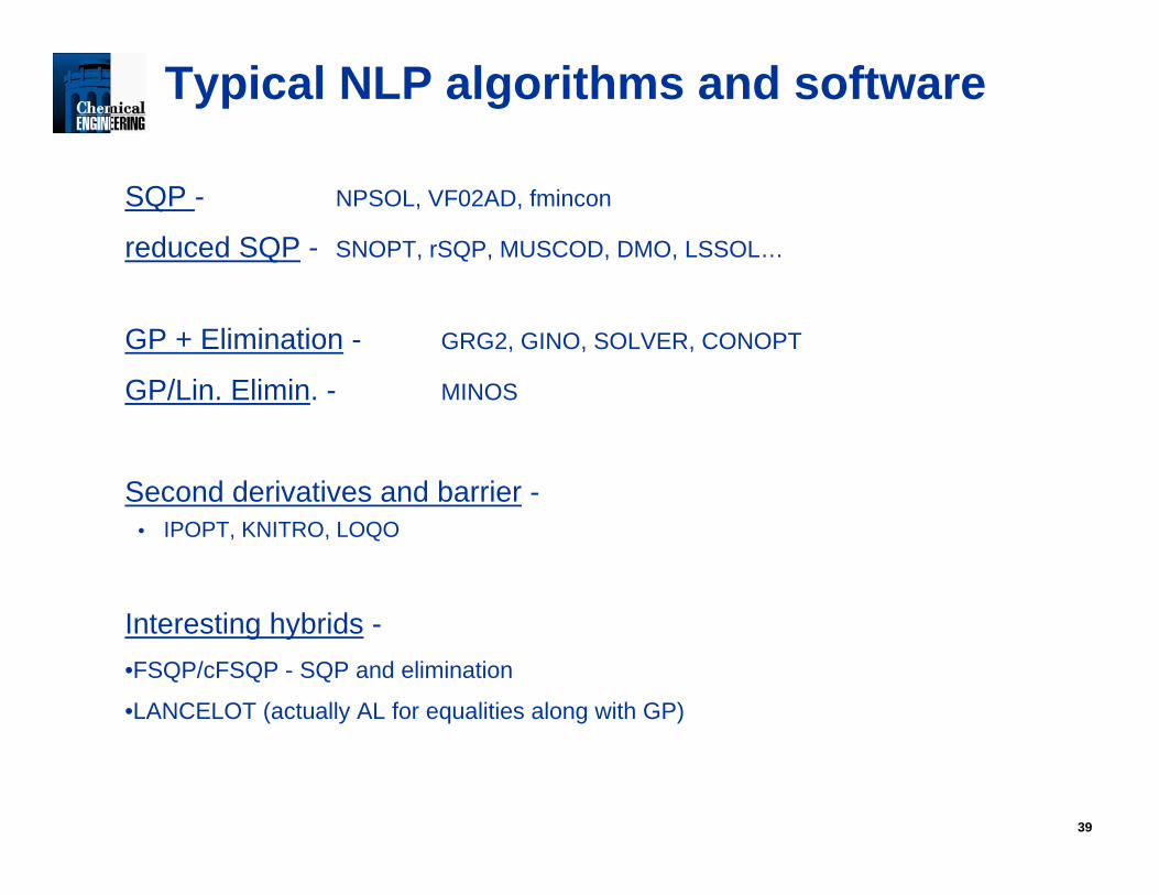
Typical NLP algorithms and software

SQP - NPSOL, VF02AD, fmincon

reduced SQP - SNOPT, rSQP, MUSCOD, DMO, LSSOL…

GP + Elimination - GRG2, GINO, SOLVER, CONOPT

GP/Lin. Elimin. - MINOS

Second derivatives and barrier -• IPOPT, KNITRO, LOQO

Interesting hybrids -•FSQP/cFSQP - SQP and elimination

•LANCELOT (actually AL for equalities along with GP)

40

Comparison of NLP Solvers: Data Reconciliation (2004)

0.01

0.1

1

10

100

0 200 400 600

Degrees of Freedom

CPU

Tim

e (s

, nor

m.)

LANCELOT

MINOS

SNOPT

KNITRO

LOQO

IPOPT

0

200

400

600

800

1000

0 200 400 600Degrees of Freedom

Itera

tions

LANCELOTMINOSSNOPTKNITROLOQOIPOPT

41

Comparison of NLP solvers(latest Mittelmann study)

117 Large117 Large--scale Test Problemsscale Test Problems500 500 -- 250 000 variables, 0 250 000 variables, 0 –– 250 000 constraints250 000 constraints

Mittelmann NLP benchmark (10-26-2008)

0

0.1

0.2

0.3

0.4

0.5

0.6

0.7

0.8

0.9

1

0 2 4 6 8 10 12

log(2)*minimum CPU time

frac

tion

solv

ed w

ithin

IPOPTKNITROLOQOSNOPTCONOPT

arki0009 6220 5924 86 148 1141 fail 1143 54ex8_2_2 7510 1943 4 4 i 10 44 34ex8_2_3 15636 3155 8 8 i 31 78 87

-----------------------------------------------------------------------------8 qcqp500-2c 500 178 933 95 383 1051 65 4882$ qcqp500-3c 500 120 889 136 784 1313 204 3346

qcqp750-1c 750 245 992 77 510 685 78 2829qcqp750-2c 750 138 1888 195 3394 t 637 tqcqp1000-1c 1000 154 592 25 203 549 618 256qcqp1000-2c 1000 5107 783 243 869 297 1080 2840qcqp1500-1c 1500 10508 t t 4888 t fail tqcqp500-2nc 500 178 1052 74 569 1002 175 4695qcqp500-3nc 500 120 698 120 929 1348 257 3200qcqp750-1nc 750 245 1039 64 542 681 fail 2765qcqp750-2nc 750 138 3629 195 3617 t 760 tqcqp1000-1nc 1000 154 294 2877 1122 503 1870 594qcqp1000-2nc 1000 5107 849 198 884 307 908 2717qcqp1500-1nc 1500 10508 4127 t 4675 t fail t

-----------------------------------------------------------------------------9 nql180 162001 130080 fail 761 5605 t fail t$ qssp60 29525 14581 8 20 t 18 t fail

qssp180 261365 139141 479 4448 m 338 t fail-----------------------------------------------------------------------------10 WM_CFx 8520 9826 5438 3552! 2708 fail 8821 7088

WM_CFy 8520 9826 t 4062! 17866 fail fail 45925Weyl_m0 1680 2049 t 2772! fail 4191 fail fail

NARX_CFy 43973 46744 1285 226! fail m fail tNARX_Weyl 44244 45568 t 8291! fail fail fail fail

===========================================================================

arki0009 6220 5924 86 148 1141 fail arki0009 6220 5924 86 148 1141 fail 1143 541143 54ex8_2_2 7510 1943 4 4 i 10 ex8_2_2 7510 1943 4 4 i 10 44 3444 34ex8_2_3 15636 3155 8 8 i 31 ex8_2_3 15636 3155 8 8 i 31 78 8778 87

----------------------------------------------------------------------------------------------------------------------------------------------------------8 qcqp5008 qcqp500--2c 500 178 933 95 383 1051 65 42c 500 178 933 95 383 1051 65 4882882$ qcqp500$ qcqp500--3c 500 120 889 136 784 1313 204 33c 500 120 889 136 784 1313 204 3346346

qcqp750qcqp750--1c 750 245 992 77 510 685 78 21c 750 245 992 77 510 685 78 2829829qcqp750qcqp750--2c 750 138 1888 195 3394 t 637 2c 750 138 1888 195 3394 t 637 ttqcqp1000qcqp1000--1c 1000 154 592 25 203 549 618 21c 1000 154 592 25 203 549 618 25656qcqp1000qcqp1000--2c 1000 5107 783 243 869 297 1080 282c 1000 5107 783 243 869 297 1080 284040qcqp1500qcqp1500--1c 1500 10508 t t 4888 t fail 1c 1500 10508 t t 4888 t fail ttqcqp500qcqp500--2nc 500 178 1052 74 569 1002 175 42nc 500 178 1052 74 569 1002 175 4695695qcqp500qcqp500--3nc 500 120 698 120 929 1348 257 33nc 500 120 698 120 929 1348 257 3200200qcqp750qcqp750--1nc 750 245 1039 64 542 681 fail 21nc 750 245 1039 64 542 681 fail 2765765qcqp750qcqp750--2nc 750 138 3629 195 3617 t 760 2nc 750 138 3629 195 3617 t 760 ttqcqp1000qcqp1000--1nc 1000 154 294 2877 1122 503 1870 51nc 1000 154 294 2877 1122 503 1870 59494qcqp1000qcqp1000--2nc 1000 5107 849 198 884 307 908 272nc 1000 5107 849 198 884 307 908 271717qcqp1500qcqp1500--1nc 1500 10508 4127 t 4675 t fail 1nc 1500 10508 4127 t 4675 t fail tt

----------------------------------------------------------------------------------------------------------------------------------------------------------9 nql180 162001 130080 fail 761 5605 t 9 nql180 162001 130080 fail 761 5605 t fail tfail t$ qssp60 29525 14581 8 20 t 18 $ qssp60 29525 14581 8 20 t 18 t failt fail

qssp180 261365 139141 479 4448 m 338 qssp180 261365 139141 479 4448 m 338 t failt fail----------------------------------------------------------------------------------------------------------------------------------------------------------10 10 WM_CFxWM_CFx 8520 9826 5438 3552! 2708 fail 8821 8520 9826 5438 3552! 2708 fail 8821 70887088

WM_CFyWM_CFy 8520 9826 t 4062! 17866 fail 8520 9826 t 4062! 17866 fail failfail 4592545925Weyl_m0 1680 2049 t 2772! fail 4191 Weyl_m0 1680 2049 t 2772! fail 4191 fail fail failfail

NARX_CFyNARX_CFy 43973 46744 1285 226! fail m fail 43973 46744 1285 226! fail m fail ttNARX_WeylNARX_Weyl 44244 45568 t 8291! fail 44244 45568 t 8291! fail failfail failfail failfail

==========================================================================================================================================================

Limits FailLimits FailIPOPT 7 2IPOPT 7 2KNITRO 7 0KNITRO 7 0LOQO 23 4LOQO 23 4SNOPT 56 11SNOPT 56 11CONOPT 55 11CONOPT 55 11

42

NLP Summary

Widely used - solving nonlinear problems with thousands of variables and superbasics routinely

Exploiting sparsity and structure leads to solving problems with millions of variables (and superbasics)

Availability of structure and second derivatives is the key.

Global and fast local convergence properties are well-known for many (but not all algorithms)

Exceptions: LOQO, MINOS, CONOPT, GRG

43

Current Challenges

- Exploiting larger problems in parallel (shared and distributed memory),

- Irregular problems (e.g., singular problems, MPECs)

- Extracting accurate first and second derivatives from codes...

- Embedding robust NLPs within MINLP and global solvers in order to quickly detect infeasible solutions in subregions