1

Optimal Crane Scheduling

Ionu AronIBM Watson Lab

Latife Genç Kaya, John HookerCarnegie Mellon University

Iiro Harjunkoski, Marco FahlABB Group

November 2006

2

Thanks to…

• PITA – Pennsylvania Infrastructure Technology Alliance.

• ABB Group

3

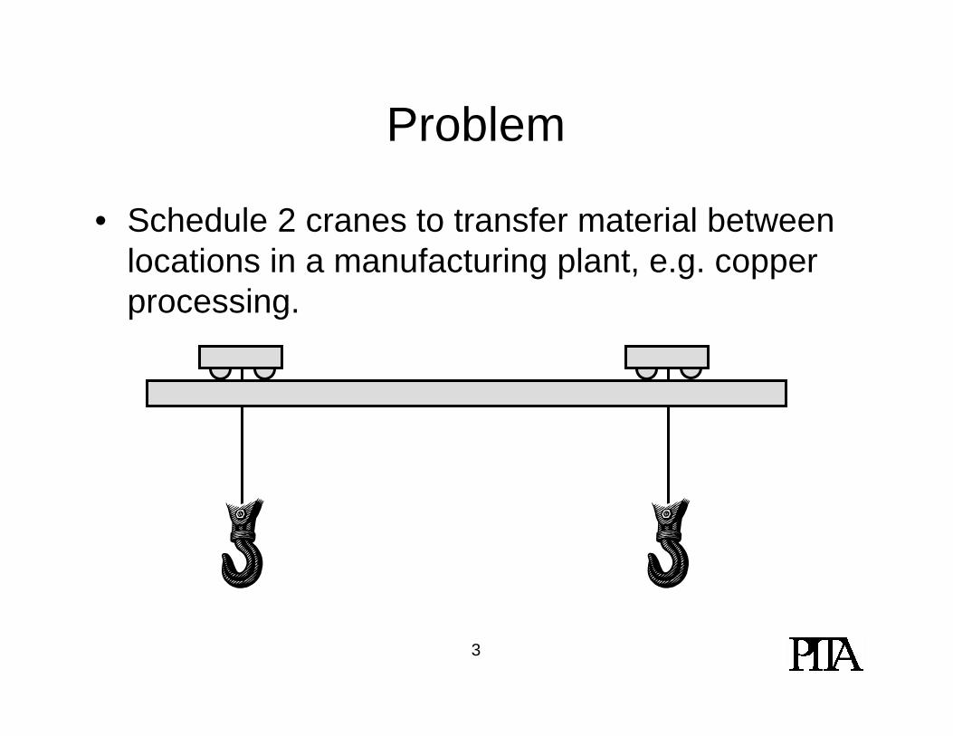
Problem

• Schedule 2 cranes to transfer material between locations in a manufacturing plant, e.g. copper processing.

4

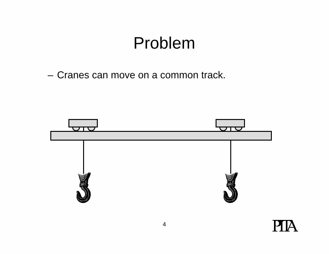
Problem

– Cranes can move on a common track.

5

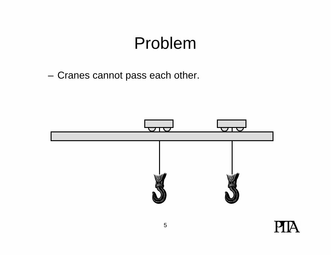
Problem

– Cranes cannot pass each other.

6

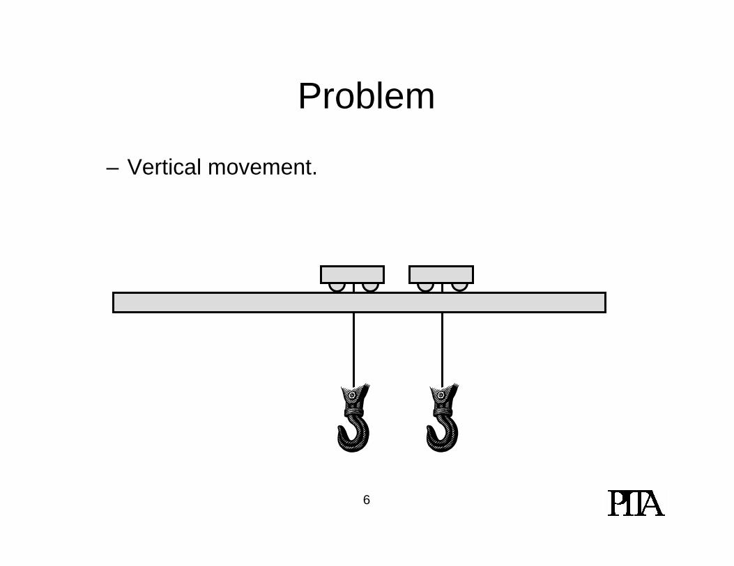
Problem

– Vertical movement.

7

Problem

– Vertical movement.• Horizontal and vertical movement can be simultaneous.

8

Problem

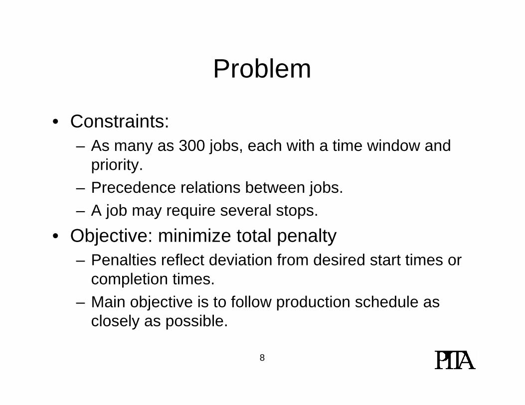
• Constraints:– As many as 300 jobs, each with a time window and

priority.– Precedence relations between jobs.– A job may require several stops.

• Objective: minimize total penalty– Penalties reflect deviation from desired start times or

completion times.– Main objective is to follow production schedule as

closely as possible.

9

Problem

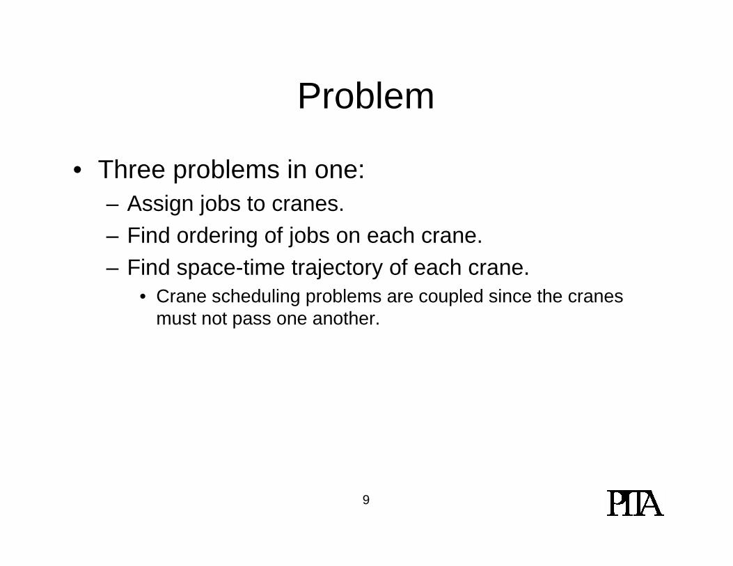
• Three problems in one:– Assign jobs to cranes.– Find ordering of jobs on each crane.– Find space-time trajectory of each crane.

• Crane scheduling problems are coupled since the cranes must not pass one another.

10

Two-phase Algorithm

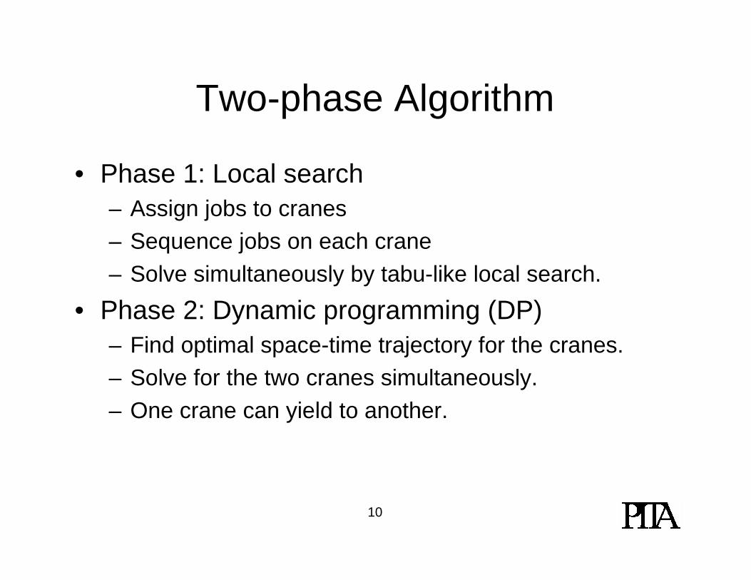
• Phase 1: Local search– Assign jobs to cranes– Sequence jobs on each crane– Solve simultaneously by tabu-like local search.

• Phase 2: Dynamic programming (DP)– Find optimal space-time trajectory for the cranes.– Solve for the two cranes simultaneously.– One crane can yield to another.

11

Local Search

• Neighborhood is defined by two types of moves.– Change assignment– Change sequence

• Evaluation of moves– Use an approximate evaluation function to limit

neighborhood.– Check best moves with DP (phase 2).

12

Dynamic Programming

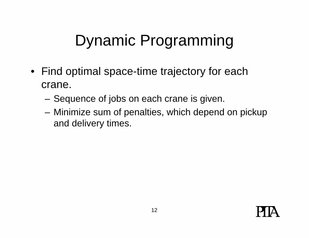
• Find optimal space-time trajectory for each crane.– Sequence of jobs on each crane is given.– Minimize sum of penalties, which depend on pickup

and delivery times.

13

Dynamic Programming

• Each job consists of one or more “segments.”– Order of segments within a job is fixed.

• Each segment consists of loading, movement to another position, unloading.

• Given for each segment:– Loading and unloading positions.– Time required to load, unload.– Min time for crane movement.

14

Dynamic Programming

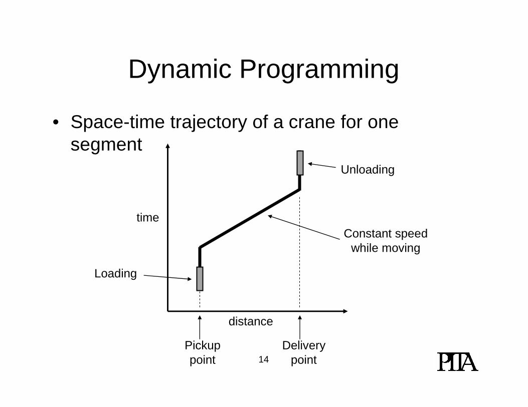
• Space-time trajectory of a crane for one segment

time

distance

Pickup point

Delivery point

Loading

Unloading

Constant speed while moving

15

Dynamic Programming

• High resolution needed to track crane motion.– Time horizon: hours– Granularity: 10-second intervals

• Thousands of discrete times

– Cranes are stationary most of the time• While loading/unloading• But motion is fast when it occurs (e.g. 1 meter/sec)

– Feasibility is main issue• No obvious role for approximate DP

16

Dynamic Programming

• Main issue: size of state space.

• State variables:– Position of each crane on track.– How long each crane has been loading/unloading.– Current segment in process for each crane

• Negative number if on the way to load the segment.• Positive number if loading, unloading, or on the way to

unload.

17

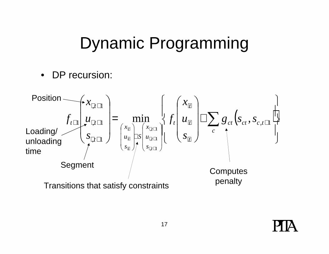
Computes penalty

( )

+

=

∑ +

⋅

⋅

⋅

∈

+⋅

+⋅

+⋅

+

+⋅

+⋅

+⋅

⋅

⋅

⋅ ctcctct

t

t

t

t

s

u

x

S

s

u

x

t

t

t

t ssg

s

u

x

f

s

u

x

f

t

t

t

t

t

t1,

1,

1,

1,

1 ,min

1,

1,

1,

Dynamic Programming

• DP recursion:

Transitions that satisfy constraints

Position

Loading/unloading time

Segment

18

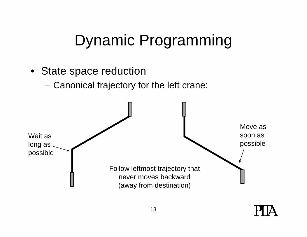
Dynamic Programming

• State space reduction– Canonical trajectory for the left crane:

Wait as long as possible

Move as soon as possible

Follow leftmost trajectory that never moves backward (away from destination)

19

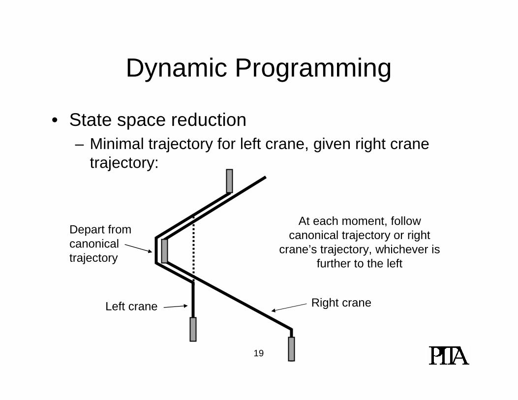
Dynamic Programming

• State space reduction– Minimal trajectory for left crane, given right crane

trajectory:

Depart from canonical trajectory

At each moment, follow canonical trajectory or right

crane’s trajectory, whichever is further to the left

Left crane Right crane

20

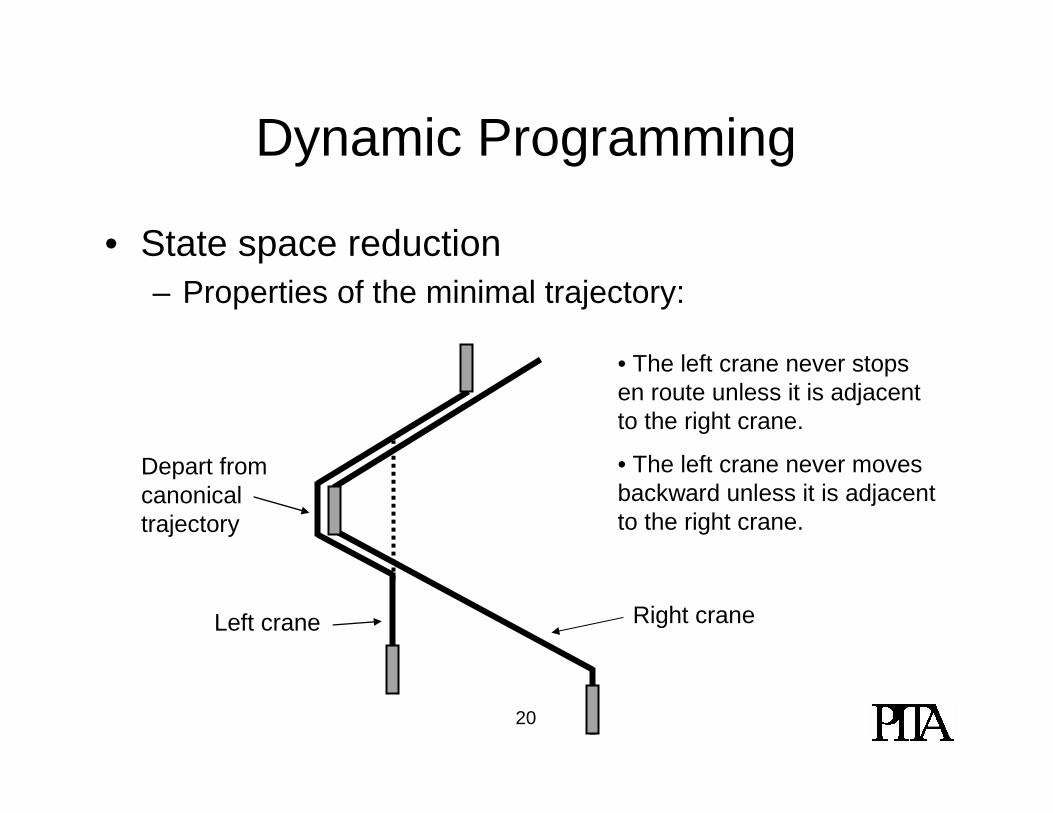
Dynamic Programming

• State space reduction– Properties of the minimal trajectory:

• The left crane never stops en route unless it is adjacent to the right crane.

• The left crane never moves backward unless it is adjacent to the right crane.

Depart from canonical trajectory

Left crane Right crane

21

Dynamic Programming

• State space reduction– Theorem: Given optimal trajectories for both cranes,

either crane’s trajectory in each segment can be replaced by a minimal trajectory without sacrificing optimality or feasibility.

22

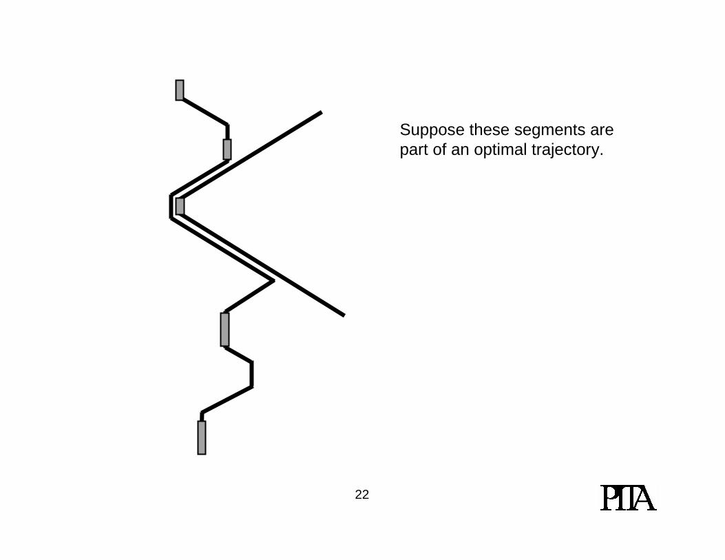
Suppose these segments are part of an optimal trajectory.

23

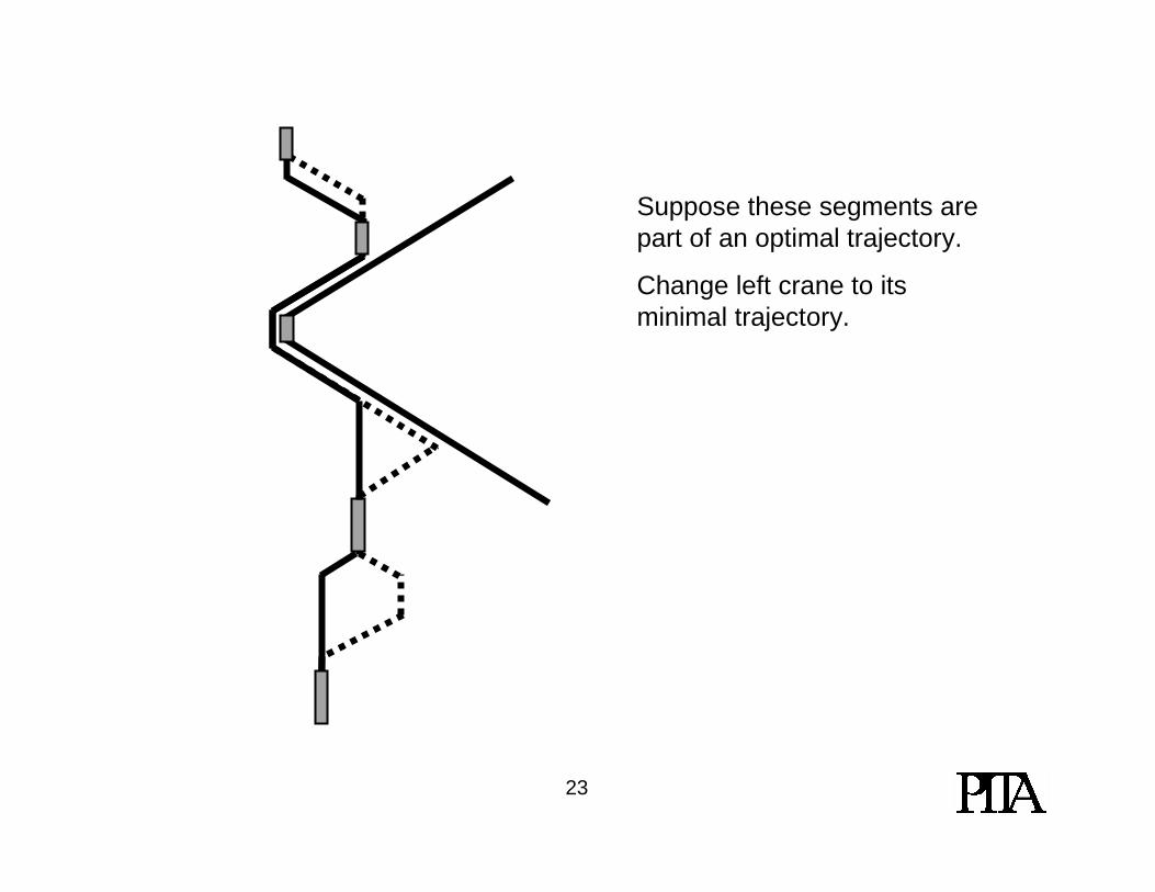
Suppose these segments are part of an optimal trajectory.

Change left crane to its minimal trajectory.

24

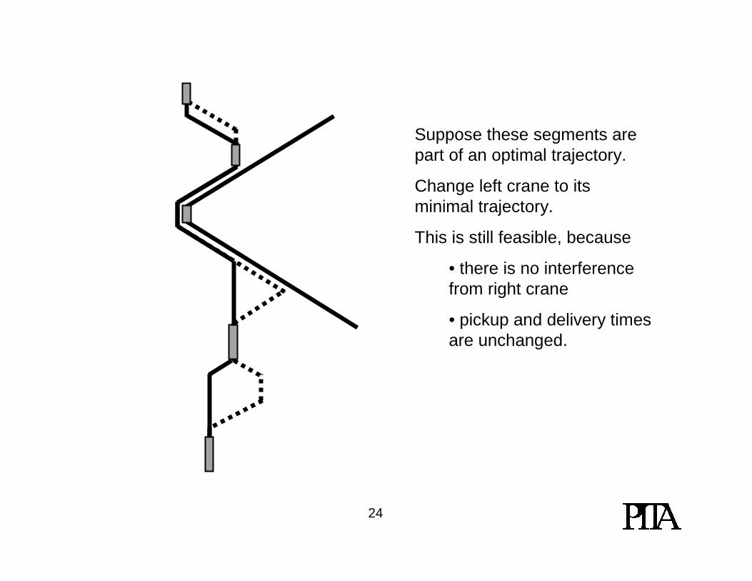
Suppose these segments are part of an optimal trajectory.

Change left crane to its minimal trajectory.

This is still feasible, because

• there is no interference from right crane

• pickup and delivery times are unchanged.

25

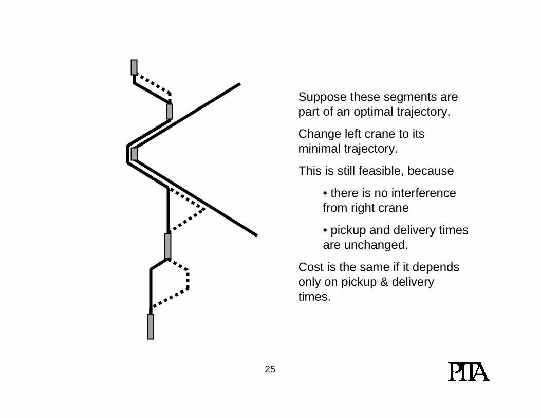
Suppose these segments are part of an optimal trajectory.

Change left crane to its minimal trajectory.

This is still feasible, because

• there is no interference from right crane

• pickup and delivery times are unchanged.

Cost is the same if it depends only on pickup & delivery times.

26

Dynamic Programming

• State space reduction– Corollary: Exclude state transitions in which a crane

stops en route, or moves backward, unless it is adjacent to the other crane.

27

Dynamic Programming

• State space reduction– Since the main objective is to follow the production

schedule, fairly tight time windows can be used. – This reduces the number of jobs in the state space at

any one time.– If necessary, time horizon can be split into segments

to be solved separately.

28

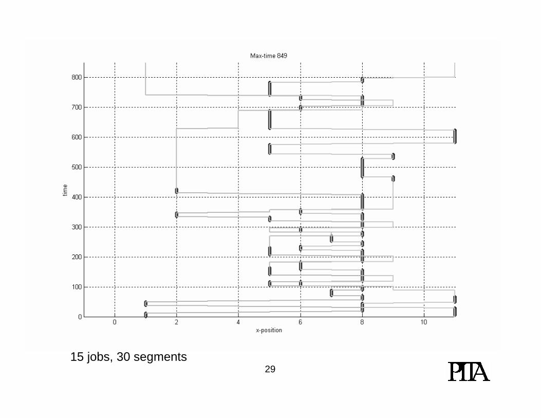
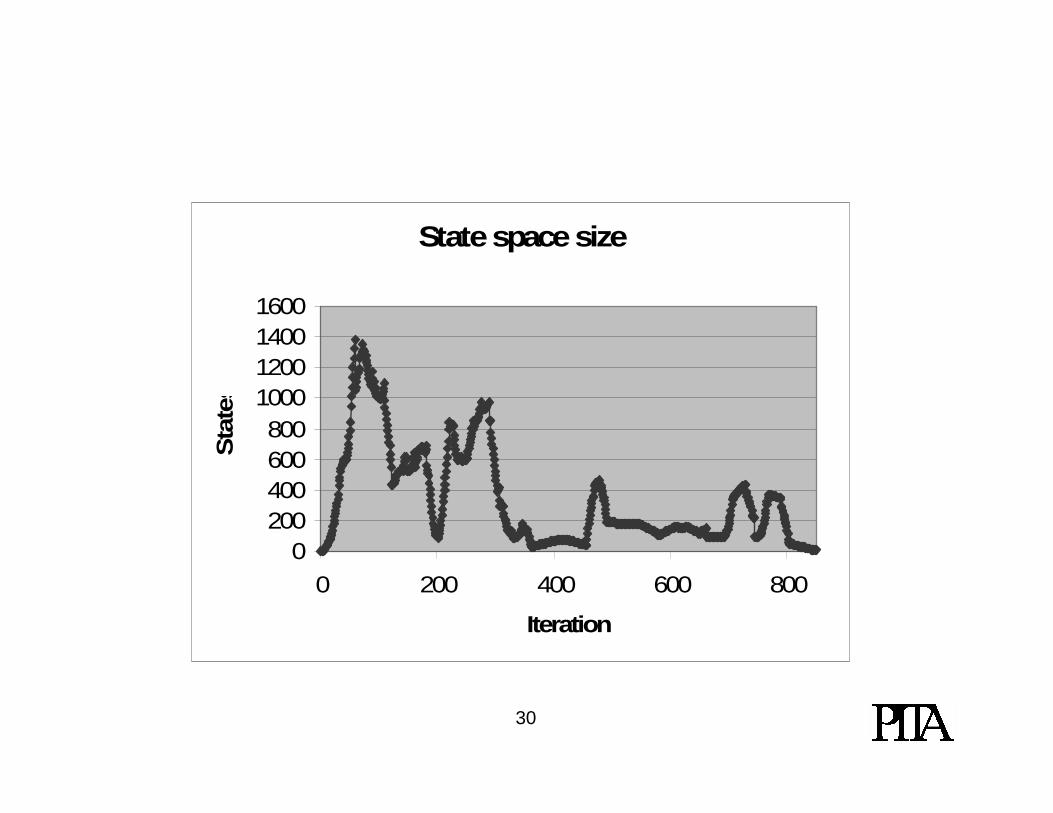
Dynamic Programming

• Preliminary computational results.– 10 crane positions (realistic).– Penalize time lapse between release time and pickup.– Minimize sum of penalties.– Theoretical maximum number of states in any given

stage is approximately 108 – 109.

29

• Computational results --- to be added.

15 jobs, 30 segments

30

State space size

0200400600800

1000120014001600

0 200 400 600 800

Iteration

Sta

tes

31

Precedence Constraints

• The crane problem has more complex precedence constraints than ordinarily occur in scheduling problems.– Hard precedence constraints apply to groups of jobs.– Soft precedence constraints are enforced by

imposing penalties.– Some precedence constraints are enforced by

combinations of hard and soft constraints.

32

Precedence Constraints

• Hard constraint– Let S, T be sets of jobs.– S < T means that all jobs in S assigned to a given

crane must run before any job in T assigned to that crane.

• Jobs within S may occur in any order, similarly for T.• {cranes that perform the jobs in S }

= {cranes that perform the jobs in T }• Jobs in neither S nor T can run between S and T.

33

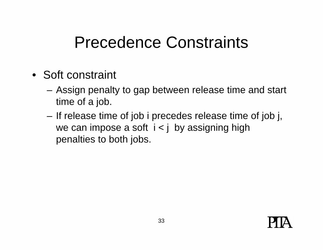
Precedence Constraints

• Soft constraint– Assign penalty to gap between release time and start

time of a job.– If release time of job i precedes release time of job j,

we can impose a soft i < j by assigning high penalties to both jobs.

34

Precedence Constraints

• Consecutive jobs– Suppose S < T and S, T should occur consecutively.

• There should be no jobs i, j, k assigned to the same crane such that i ∈ S, j ∉ S∪T, k ∈ T, and j runs between i and k.

– To enforce this:• Impose S < T.• Give jobs in S very similar release times to jobs in T.• Impose high penalties on jobs in S, T.

35

Assignment and Sequencing

• Heuristic algorithm:– Form initial assignment/sequencing with simple

nearest job heuristic.– Call DP repeatedly with increasing time windows until

feasible solution is found or max time windows reached.

– Move to random neighboring solution • Consider neighbors with estimated penalty within

15-20% of best solution found so far.

36

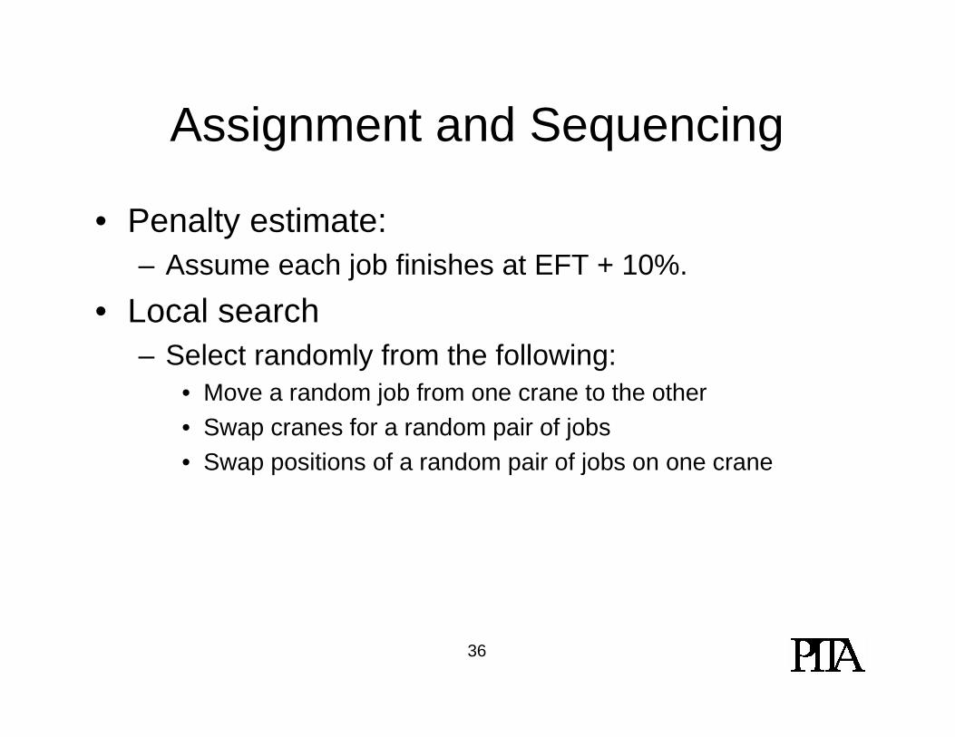
Assignment and Sequencing

• Penalty estimate:– Assume each job finishes at EFT + 10%.

• Local search– Select randomly from the following:

• Move a random job from one crane to the other• Swap cranes for a random pair of jobs• Swap positions of a random pair of jobs on one crane

37

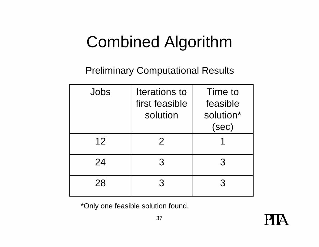
Combined Algorithm

3328

3324

1212

Time to feasible solution*

(sec)

Iterations to first feasible

solution

Jobs

Preliminary Computational Results

*Only one feasible solution found.

38

Future Work

• Generate nogood constraints from DP solution.– Identify a subsequence of jobs (assigned to the same

crane) that is responsible for infeasibility.– Create a nogood constraint that prevents heuristic

phase from assigning this subsequence to the same crane again.