Estimation and Inference in the Cointegrated System

with Stationary Covariates

Byeongseon Seo ∗

Texas A&M University †

October 2004

∗I would like to thank Bruce Hansen, Joon Park, and Pentti Saikkonen for helpful comments and sugges-

tions. The author gratefully acknowledges financial support from the Korea Research Foundation.†Department of Economics, College Station, TX 77843-4228, USA. E-mail: seo@econmail.tamu.edu.

Phone: 979-845-7307. Fax: 979-847-8757.

1

Abstract

This paper explores the asymptotic distribution of the cointegrating vector estimator

and statistical inference on cointegration in the vector error correction model (ECM) with

stationary covariates, which are generated from the stationary VAR process. First, the

asymptotic distribution of the cointegrating vector estimator is locally asymptotically mixed

normal, and asymptotic efficiency improves as the magnitude of the covariate effect increases.

Second, the asymptotic distribution of the Wald and the LR statistics for cointegration

is a mixed combination of the chi-squared and the nonstandard distributions. The null

distribution approaches the chi-squared distribution and the power of the cointegration tests

improves significantly as the covariate effect increases. Monte Carlo simulations show that

the bootstrap inference, as well as the asymptotic inference, generate moderate size and

power performances. Third, the limiting distributions of the cointegrating vector estimator

and the cointegration test depend on the stationary covariates, and thus the omission of the

covariates leads to the departure from the existing distribution theory, which does not allow

for stationary covariates.

Key words: Cointegration Test; Efficient Estimation; Stationary Covariates

JEL classification: C12; C32

2

1 Introduction

This paper aims to explore the asymptotic theory for estimation and inference in the vector

error correction model (ECM) with stationary covariates. The stationary covariates have

been used in many economic studies to consider the effect of stationary policy variables or to

improve the model fitness on empirical grounds. However, the stationary covariates have been

disregarded or treated less importantly in the cointegrated system, and statistical inference

on the cointegrating vector and cointegration has been based on the distribution theory,

which does not allow for stationary covariates. In this paper, we allow stationary covariates

in the cointegrated system and develop the distribution theory for the cointegrating vector

estimator and inference on cointegration.

The distribution theory of the cointegrating vector estimator has been developed by

Johansen (1988, 1991), Phillips and Hansen (1990), Phillips (1991), Saikkonen (1991), and

Stock and Watson (1993). Although extensive literature exists on the cointegrating vector,

the literature on theoretical aspects of stationary covariates is still sparse. Saikkonen (1991)

considered the stationary covariates in the cointegrated regression model and has shown

that the asymptotic distribution is different from the former results. This study explores the

distribution of the cointegrating vector estimator in the ECM with stationary covariates.

Statistical inference on the existence of the cointegrating relationship must be one of

the crucial issues for the models with nonstationary variables. Johansen (1988, 1991) has

developed the likelihood ratio (LR) test statistic for cointegration in the ECM. Because the

economic models often use stationary variables in the ECM, it is necessary to develop the

appropriate distribution theory. Seo (1998) has shown that the asymptotic distribution of

the cointegration rank test depends on the covariate effect. However, the cointegration tests

have been based on the nonstandard distribution, which does not allow for the covariate

effect. In this study, we propose the Wald test statistic for cointegration and develop the

methods to implement proper inference on cointegration based on the bootstrapping and the

asymptotic theory.

We also consider the cointegrating vector estimator and inference on cointegration in

3

the misspecified model, which neglects the stationary covariates. The stationary covari-

ates have been overlooked in the model with nonstationary variables, and the effect of the

omitted stationary covariates on the distribution of the cointegrating vector has not been

explored. Here, we develop the associated distribution theory for estimation and inference

in the misspecified model, and thereby contribute to the literature.

The stationary covariates provide information which affects the asymptotic theories of

the cointegrating vector estimator and the tests for cointegration. First, the asymptotic

distribution of the cointegrating vector estimator depends on the effect of stationary covari-

ates, and asymptotic efficiency improves as the magnitude of the covariate effect increases.

Second, the asymptotic distribution of the Wald and the LR statistics for cointegration is

a mixed combination of the chi-squared and the nonstandard distributions. The null dis-

tribution approaches the chi-squared distribution, and the power of the cointegration tests

improves significantly as the covariate effect increases. Monte Carlo simulations show that

the bootstrap inference, as well as the asymptotic inference, generate moderate size and

power performances. Third, the asymptotic distributions of the cointegrating vector estima-

tor and the cointegration test depend on the stationary covariates, and thus the omission of

the covariates leads to the departure from the existing distribution theory, which does not

allow for stationary covariates.

Our model is related to the partial system or the structural error correction model because

the partial system is specified by conditioning some endogenous variables of interest on the

other remaining variables. In this respect, the literature on the structural error correction

model such as Boswijk (1995), Ericsson (1995), Johansen (1992), and Harbo et al. (1998)

is worth mentioning. However, the cointegrating relationship of our model does not involve

the stationary covariates, and thus our model is different from the partial system.

Hansen (1995) and Elliot and Jansson (2003) considered the unit root test with the

stationary covariates. The stationary covariates help to increase the power of the unit root

tests. Here, we extend the univariate analysis to the cointegration tests. The power of the

cointegration tests has been evaluated by Kremers et al. (1992), where the power of the

cointegration tests depends on the error correction process. In this paper, we show that

4

the null distribution of the cointegration tests depends on the stationary covariates, and the

covariate effect improves the power of the cointegration tests.

We use the following notation: The operation ⊗ signifies the Kronecker product, and

det(A) and tr(A) denote the determinant and the trace of matrix A, respectively. We denote

vec(A) as the column-stacking operator and |A| as the Euclidean norm of the matrix A.

Also, we denote →p as convergence in probability and ⇒ as weak convergence of probabil-

ity measures. W (r) = BM(Ω) represents a multivariate Brownian motion with long-run

variance Ω.∫

W is an abbreviated form of∫ 1

0W (r)dr, W is W (r), [·] is the integer part

operator, and L is the lag operator.

The next section deals with the model and assumptions. Section 3 provides the asympto-

tic theory for the cointegrating vector estimator. Statistical inference on cointegration with

stationary covariates is analyzed in Section 4. The omission of the stationary covariates and

its effect on the cointegrating vector estimator and cointegration tests are investigated in

Section 5. The models with deterministic trends are discussed in Section 6. Section 7 pro-

vides simulation evidence on the cointegrating vector estimator and the cointegration tests.

An economic application is provided in Section 8.

2 The Model

Consider the p-dimensional nonstationary time series xt, t = 1, . . . , n, which is generated

by an error correction model (ECM). Suppose we also have the k-dimensional stationary

variable zt generated by a stationary vector autoregressive (VAR) model as follows:

∆xt = Πxt−1 +l∑

i=1

Φ11i∆xt−i + νt (1)

zt =l∑

i=1

Φ21i∆xt−i +m∑

i=1

Φ22izt−i + et (2)

where νt

et

∼ i.i.d.(

0

0

,

Σνν Σνe

Σeν Σee

).

5

The cointegrating vector β and the adjustment vector α can be estimated without loss

of efficiency, when there are no restrictions on the parameters across equations, from the

following error correction model:

∆xt = Πxt−1 +l∑

i=1

Γi∆xt−i +m∑

i=0

Ψizt−i + ut, (3)

where Π = αβ′, ut = νt − Ψ0et, Ψ0 = ΣνeΩ

−1ee , Γi = Φ11i − Ψ0Φ21i, and Ψj = −Ψ0Φ22j for

i = 1, 2, . . . , l and j = 1, 2, . . . ,m.

We assume that the error ut is a vector Martingale difference sequence (MDS) with

Σ = E(utu′t) < ∞. Note that the ECM error ut is uncorrelated with the VAR error of the

stationary covariates.

Our model is the standard ECM with the stationary covariates. In empirical studies,

the estimated errors often do not satisfy the regularity conditions, and they are correlated

with stationary economic variables. Also, the stationary policy variables may be considered

in macroeconomic models. Thus, the stationary covariates have been used in many studies

such as Johansen and Juselius (1992), Baba et al. (1992), and Juselius (1995).

Our model is related to the partial system or the conditional error correction model

because the partial system can be specified by conditioning some endogenous variables of in-

terest on the other remaining variables. However, the cointegrating relationship of our model

does not involve the stationary covariates, and thus our model is different from the partial

system. Our model assumes that the covariates are weakly exogenous to the cointegrating

relationship, as in the partial systems. The efficiency of the estimators in the partial system

depends on weak exogeneity of the conditioning variables, and this condition can be verified

by using the standard testing methods, as discussed by Johansen (1992).

The ECM (3) and the VAR model (2) can be written as follows:

∆xt = Πxt−1 + Γ(L)∆xt + Ψ(L)zt + ut

zt = Φ1(L)∆xt + Φ2(L)zt + et,

where Γ(L) =∑l

i=1 ΓiLi, Ψ(L) =

∑mi=0 ΨiL

i, Φ1(L) =∑l

i=1 Φ1iLi, and Φ2(L) =

∑mi=1 Φ2iL

i.

6

If we define Π(L) = (1−L)I −ΠL−Γ(L)(1−L)−Ψ(L)(I −Φ2(L))−1Φ1(L)(1−L), the

ECM (3) can be written as

Π(L)xt = vt, (4)

where vt = ut + Ψ(L)(I − Φ2(L))−1et.

Assumption 1 (a) All roots of det(Π(L)) = 0 lie outside or on the unit circle.

(b) All roots of det(I − Φ2(L)) = 0 lie outside the unit circle.

To show the main results, we use the representation theorem by Engle and Granger

(1987).

Theorem 1 (The Granger Representation Theorem)

Suppose Assumption 1 holds and Π = αβ′, where α and β are p×r full column rank matrices.

If α⊥ and β⊥ are p × (p − r) full column rank matrices such that α′⊥α = 0 and β

′⊥β = 0,

then the error correction model (3) can be represented by

(a)

∆xt = C(L)vt,

with C(1) = β⊥(α′⊥Π∗(1)β⊥)−1α

′⊥, where Π∗(L) = Π(L)−Π(1)

1−L,

(b)

xt = C(1)t∑

i=1

vi + C∗(L)vt,

where C∗(L) = C(L)−C(1)1−L

, and

(c)

wt = β′xt = β

′C∗(L)vt.

The proof comes directly from Engle and Granger (1987) and Johansen (1991), although

our model allows for stationary covariates. The data generating process xt has stochastic

trends and a stationary component. If Π = αβ′, the null space of C(1) is spanned by the

7

cointegration space. Hence, β′C(1) = 0 and C(1)α = 0. The stochastic trends in xt are

eliminated if we multiply the cointegrating vector. Thus, the cointegrating relationship β′xt

is stationary.

Also, from the representation theorem, the stationary covariate zt has the following rep-

resentation:

zt = D1(L)ut + D2(L)et,

where D1(L) = (I−Φ2(L))−1Φ1(L)C(L) and D2(L) = (I−Φ2(L))−1[I+Φ1(L)C(L)Ψ(L)(I−Φ2(L))−1].

We define Ft−1 as the σ-field generated by xt−i, zt, zt−i, i = 1, 2, · · ·. We denote Gt−1 as

the sub-σ-field generated by xt−i, zt−i, i = 1, 2, · · ·, which satisfies Gt−1 ⊂ Ft−1. We assume

the following conditions:

Assumption 2 (a) E(ut|Ft−1) = 0 and E(et|Gt−1) = 0.

(b) supt E|ηt|q < ∞ for some q > 2, where ηt = (u′t, e

′t)′.

(c)∑∞

k=1 k|Bk| < ∞, where vt = ut +B(L)et = ut +∑∞

k=0 BkLket and B(L) = Ψ(L)(I −

Φ2(L))−1.

(d)∑∞

k=1 k2|Ck| < ∞, where ∆xt = C(L)vt =∑∞

k=0 Ckvt−k.

(e)∑∞

k=1 k|D1k| < ∞ and∑∞

k=1 k|D2k| < ∞, where Dj(L) =∑∞

k=0 DjkLk for j = 1, 2.

Assumption 2-(a) implies that the error process ηt = (u′t, e

′t)′allows for conditional het-

eroskedasticity. Assumptions 2-(b) and (d) imply that the process ∆xt, wt is uniformly 2+

bounded. In the same way, the process zt is uniformly 2+ bounded under Assumptions

2-(b) and (e).

Lemma 1 Under Assumptions 1-2,

n−1/2

∑[nr]t=1 ut

n−1/2∑[nr]

t=1 vt

⇒

U(r)

V (r)

= BM(

Σ Σ

Σ Ωvv

),

where Ωvv = Σ + Ψ(1)(I − Φ2(1))−1Σee(I − Φ2(1))−1′Ψ′(1).

8

3 Cointegrating Vector Estimator

We assume that the matrix Π in (3) is of rank r (0 < r < p). Thus, there exist p × r

full-column rank matrices α and β which satisfy the following:

Π = −Π(1) = αβ′.

The cointegrating relationship β′xt is stationary as defined in Engle and Granger (1987).

Our model allows for stationary covariates zt, and it is assumed that the stationary covariates

are weakly exogenous, as defined by Engle et al. (1983), to the cointegrating relationship.

As discussed in Johansen (1992) and Boswijk (1995), the cointegrating vector β can be

estimated efficiently in the model (3) under weak exogeneity.

We use the following normalization of the cointegrating vector:

wt(β) = x1t + β′x2t, (5)

where x1t is r-dimensional, x2t is (p− r)-dimensional, and β is a (p− r)× r matrix.

The cointegrating vector can be identified from the normalization. Our representation of

the cointegrating relationship has been used in many studies such as Phillips (1991).

Let st = (s′1t, s

′2t)

′, where s1t = (∆x

′t−1, ∆x

′t−2, . . . , ∆x

′t−l)

′and s2t = (z

′t, z

′t−1, . . . , z

′t−m)

′.

The ECM (3) can be written as follows:

∆xt = αwt−1(β) + Γs1t + Ψs2t + ut,

where Γ = (Γ1, Γ2, . . . , Γl) and Ψ = (Ψ0, Ψ1, . . . , Ψm).

We define the parameter vector θ = (vec(β)′, θ

′2)′ ∈ Θ, where θ2 = vec(α, Γ, Ψ, Σ). We

denote θ0 as the true parameter value.

Under the auxiliary condition ut ∼ N(0, Σ), the likelihood function can be defined as

follows:

Ln(θ) = −n

2log |Σ| − 1

2

n∑t=1

u′t(θ)Σ

−1ut(θ), (6)

where ut(θ) is defined as ut in (3).

9

We denote θ as the MLE of θ. That is,

θ = argmaxθ∈ΘLn(θ).

The maximum likelihood estimator θ maximizes the likelihood function, and the first

order condition is given by

gn(θ) =∂Ln(θ)

∂θ= 0,

where

∂Ln(θ)

∂β=

n∑t=1

x2t−1u′tΣ

−1α,

∂Ln(θ)

∂α′=

n∑t=1

wt−1u′tΣ

−1,

∂Ln(θ)

∂Γ′=

n∑t=1

s1tu′tΣ

−1,

∂Ln(θ)

∂Ψ′ =n∑

t=1

s2tu′tΣ

−1, and

∂Ln(θ)

∂Σ−1=

n

2Σ− 1

2

n∑t=1

utu′t.

The MLE of β is denoted as β, which can be calculated by reduced rank regression (Ahn

and Reinsel, 1988) or canonical analysis (Box and Tiao, 1977). Other slope parameters can

be estimated by least squares once the cointegrating vector is estimated.

Lemma 2 Under Assumptions 1-2 and Π = αβ′,

1√n

x[nr] ⇒ C(1)V (r), (7)

where C(1) = β⊥(α′⊥Π∗(1)β⊥)−1α

′⊥.

We define (p−r)×(p−r) full-rank matrix β2⊥, which is the partitioned matrix of β⊥. We

denote C2 = β2⊥(α′⊥Π∗(1)β⊥)−1α

′⊥, which corresponds to x2t, so that 1√

nx2[nr] ⇒ C2V (r).

We define the standard Brownian motions B1(r) and B2(r) as follows: (α

′Σ−1α)−1/2α

′Σ−1 1√

n

∑[nr]t=1 ut

(α′⊥Ωvvα⊥)−1/2α

′⊥

1√n

∑[nr]t=1 vt

⇒

B1(r)

B2(r)

= BM(

I 0

0 I

). (8)

10

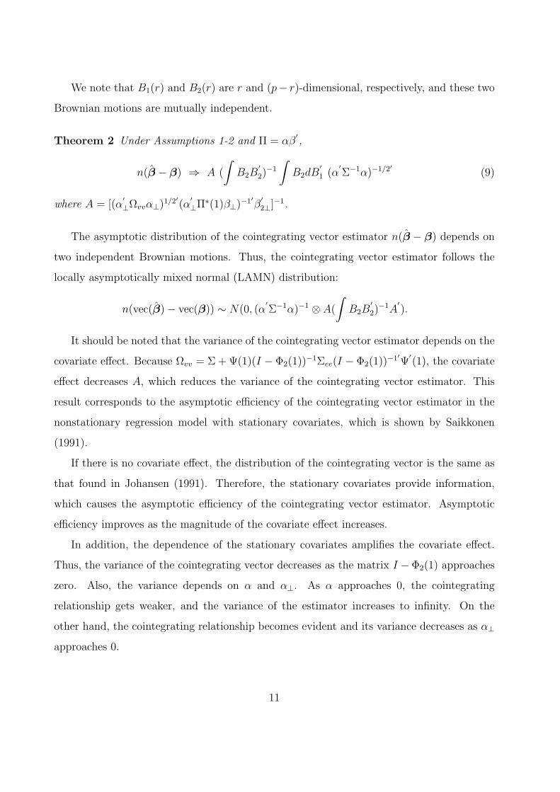
We note that B1(r) and B2(r) are r and (p− r)-dimensional, respectively, and these two

Brownian motions are mutually independent.

Theorem 2 Under Assumptions 1-2 and Π = αβ′,

n(β − β) ⇒ A (

∫B2B

′2)−1

∫B2dB

′1 (α

′Σ−1α)−1/2′ (9)

where A = [(α′⊥Ωvvα⊥)1/2′(α

′⊥Π∗(1)β⊥)−1′β

′2⊥]−1.

The asymptotic distribution of the cointegrating vector estimator n(β − β) depends on

two independent Brownian motions. Thus, the cointegrating vector estimator follows the

locally asymptotically mixed normal (LAMN) distribution:

n(vec(β)− vec(β)) ∼ N(0, (α′Σ−1α)−1 ⊗ A(

∫B2B

′2)−1A

′).

It should be noted that the variance of the cointegrating vector estimator depends on the

covariate effect. Because Ωvv = Σ + Ψ(1)(I − Φ2(1))−1Σee(I − Φ2(1))−1′Ψ′(1), the covariate

effect decreases A, which reduces the variance of the cointegrating vector estimator. This

result corresponds to the asymptotic efficiency of the cointegrating vector estimator in the

nonstationary regression model with stationary covariates, which is shown by Saikkonen

(1991).

If there is no covariate effect, the distribution of the cointegrating vector is the same as

that found in Johansen (1991). Therefore, the stationary covariates provide information,

which causes the asymptotic efficiency of the cointegrating vector estimator. Asymptotic

efficiency improves as the magnitude of the covariate effect increases.

In addition, the dependence of the stationary covariates amplifies the covariate effect.

Thus, the variance of the cointegrating vector decreases as the matrix I −Φ2(1) approaches

zero. Also, the variance depends on α and α⊥. As α approaches 0, the cointegrating

relationship gets weaker, and the variance of the estimator increases to infinity. On the

other hand, the cointegrating relationship becomes evident and its variance decreases as α⊥

approaches 0.

11

4 Inference on Cointegration

The tests for cointegration can be based on the following null and alternative hypotheses:

H0 : Π = 0 against H1 : Π 6= 0,

where Π is in model (3).

The likelihood ratio (LR) statistic for cointegration has been developed by Johansen

(1988, 1991) in the error correction model. In this paper, we propose the Wald statistic for

cointegration, which is easy to calculate and asymptotically equivalent to the LR statistic.

In particular, the Wald statistic for cointegration can be robust to the heteroskedastic errors.

The LR statistic for cointegration tends to over-reject the null hypothesis of no cointegra-

tion when the errors follow the GARCH process as in the Monte Carlo study by Lee and

Tse (1996). Because most economic variables contain heteroskedasticity, the Wald statistic

based on the robust covariance estimator can improve the finite sample properties of the

cointegration test.

We define the sample moments S00 = n−1∑n

t=1 R0tR′0t, S01 = n−1

∑nt=1 R0tR

′1t, and

S11 = n−1∑n

t=1 R1tR′1t, where

R0t = ∆xt −n∑

t=1

∆xts′t(

n∑t=1

sts′t)−1st,

R1t = xt−1 −n∑

t=1

xt−1s′t(

n∑t=1

sts′t)−1st.

The least squares estimator of Π is given by

Π′= S−1

11 S10.

The heteroskedasticity-consistent covariance estimator of nvec(Π′) is given by

Hn = (I ⊗ S−111 )

n∑t=1

(utu′t ⊗R1tR

′1t)(I ⊗ S−1

11 ),

where ut is the least squares residuals. That is, ut = ∆xt −∑n

t=1 ∆xtS′t(

∑nt=1 StS

′t)−1St,

where St = (x′t−1, s

′t)′.

12

The Wald statistic for the null hypothesis of no cointegration is given as follows:

WHn = vec(nΠ

′)′H−1

n vec(nΠ′). (10)

The standard covariance estimator, which assumes homoskedastic errors, is given by

Vn = Σ⊗ nS−111 ,

where Σ = n−1∑n

t=1 utu′t.

If the standard variance estimator is used, the Wald statistic reduces to the following:

Wn = vec(nΠ′)′(Σ⊗ nS−1

11 )−1vec(nΠ′)

= tr nΣ−1S01S−111 S10.

The likelihood ratio (LR) statistic for the null hypothesis of no cointegration can be

defined as

LRn =

p∑i=1

nλi,

where λi is the eigenvalue satisfying λ1 > λ2 > . . . > λp and for i = 1, 2, . . . , p

| λiS11 − S10S−100 S01 | = 0. (11)

Thus, the LR test statistic for cointegration is given by

LRn = tr nS−100 S01S

−111 S10. (12)

Note that S00 converges to Σ in probability under the null of no cointegration, and so

Σ. Thus, the Wald statistic, which uses the standard covariance estimator, is asymptotically

equivalent to the LR statistic.

Under the null hypothesis of no cointegration, the null space of Π amounts to the size of

xt. Thus, C(1)(= Π∗(1)−1) is a p × p matrix. As in Lemma 2, we have the following result

under the null hypothesis of no cointegration:

1√n

R1[nr] ⇒ CV (r),

where C = Π∗(1)−1.

13

Lemma 3 Under Assumptions 1-2 and the null hypothesis H0 : Π = 0, the sample moments

have the following asymptotic properties:

Σ →p Σ,

S00 →p Σ,

S10 ⇒ C

∫V dU

′, and

n−1S11 ⇒ C

∫V V

′C′.

We define the canonical correlation ρi as follows:

ρi = P′i Σ

1/2′Ω−1/2′vv Qi

where P′i Pi = 1, P

′i Pj = 0, Q

′iQi = 1, and Q

′iQj = 0 for i 6= j and i, j = 1, 2, · · · , p.

The canonical correlation matrix R can be defined as follows:

R = diag(ρ1, ρ2, · · · , ρp). (13)

The orthonormal matrices P , Q and the canonical correlation matrix R satisfy

Σ1/2′Ω−1vv Σ1/2P = PR2, and

Ω−1/2vv ΣΩ−1/2′

vv Q = QR2.

If we define W1(r) = P′Σ−1/2U(r) and W2(s) = Q

′Ω−1/2vv V (r), then

W1(r)

W2(r)

= BM

I R

R I

.

The Brownian motion W1 can be decomposed as W1 = RW2 + (I − R2)1/2W1.2, where

W1.2 and W2 are uncorrelated and hence independent Brownian motions.

Theorem 3 Under the null hypothesis H0 : Π = 0 and Assumptions 1-2 with q > 6,

WHn ⇒ tr

∫dW1W

′2(

∫W2W

′2)−1

∫W2dW

′1 ≡ W(R) (14)

14

where R is defined in equation (13). Also, we have

W(R) = tr f(R)′(

∫W2W

′2)−1 f(R), (15)

where f(R) =∫

W2dW′2R+

∫W2dW

′1.2(I−R2)1/2, and W1.2 and W2 are independent standard

Brownian motions.

Theorem 3 uses the condition up to the sixth finite moment to show the asymptotic

theory for the Wald statistic for cointegration with the heteroskedasticity-robust covariance

estimator. The condition with 2+ finite moment is sufficient if the cointegration test is based

on the standard covariance estimator, which assumes time-invariant variance.

The asymptotic distribution of the Wald statistic is equivalent to that of the LR statistic,

which has been found by Seo (1998). The Wald statistic, which uses the heteroskedasticity-

robust covariance estimator, has the same asymptotic distribution as the Wald statistic that

is based on the standard covariance estimator. Although the asymptotic distribution of the

Wald statistic for cointegration is invariant to the heteroskedastic errors, the small sample

properties of the cointegration tests depend on heteroskedastic errors. In particular, the stan-

dard residual bootstrap inference on cointegration depends heavily on the error condition.

Because most economic variables contain time-varying conditional variance, the finite sample

performance of the cointegration tests can be improved by using the heteroskedasticity-robust

covariance estimator.

We note that the asymptotic distribution depends on two correlated Brownian motions.

If there is no covariate effect, then Brownian motions are collinear (R = I) and the Wald

statistic has the following asymptotic distribution:

W(I) = tr

∫dW2W

′2(

∫W2W

′2)−1 ∫

W2dW′2, (16)

which is the same nonstandard distribution found by Johansen (1988, 1991).

If W1(r) and W2(r) are independent (R = 0), the stochastic functional∫

dW1.2⊗W2 fol-

lows a locally asymptotically mixed normal distribution with covariance matrix I⊗∫W2W

′2.

In this case, the Wald statistic is asymptotically chi-squared with p2 degrees of freedom.

Therefore, the distribution of the Wald statistic is a mixed combination of the nonstandard

15

and the chi-squared distributions. The limiting distribution approaches the chi-squared dis-

tribution as the magnitude of the covariate effect increases.

Hansen (1995) has shown that the asymptotic distribution of the ADF unit root test

with stationary covariates is a combination of the standard normal and the Dickey-Fuller

nonstandard distributions. This paper extends the univariate analysis to the cointegration

tests in the vector error correction model.

Because the stationary covariates affect the asymptotic distribution of the cointegration

test, inference on cointegration depends on the canonical correlation. The tabulated critical

values, which assume the nonstandard distribution found by Johansen (1988, 1991), do not

allow for the covariate effect. This paper proposes two methods to implement inference on

cointegration.

The first method simulates the null distribution by using the estimated canonical corre-

lation. Because the matrix R is the canonical correlation of two innovations U(r) and V (r),

it can be estimated from the long-run variance of ut, vt, where ut, vt is the estimated

error of ut, vt.The long-run variance of vt can be estimated as follows:

Ωvv = Σ + Ψ(1)(I − Φ2(1))−1Σee(I − Φ2(1))−1′Ψ′(1),

where Σ = n−1∑n

t=1 utu′t.

The canonical correlation estimates ρi for i = 1, 2, · · · , p can be calculated from the

following:

| ρ2i I − Σ1/2′Ω−1

vv Σ1/2 |= 0.

The null distribution can be simulated by using the estimated canonical correlations, and

the p-values can be calculated by simulation.1

The second method is based on the bootstrap inference, which does not require estima-

tion of the canonical correlation. In this paper, we consider the standard residual bootstrap

algorithm. The residual bootstrap approximates the sampling distribution of the test statis-

tic using the null model and the parameter estimates obtained under the null hypothesis.

1A Gauss program which performs the necessary simulation can be provided upon request.

16

To implement the bootstrap inference, we estimate the error correction model (3) and the

VAR model (2). The VAR lag-lengths can be selected by the AIC or the BIC.

The resampled residuals ubt and eb

t are randomly drawn from the sample residuals, and

then xbt and zb

t can be constructed using the parameter estimates and the resampled residuals.

The W b statistic can be calculated for each resampled data set, and then we obtain the

bootstrap p-value, which is the probability that the simulated statistic exceeds the sample

Wald statistic. If the p-value is less than the size chosen, then we reject the null hypothesis

in favor of the alternative of the presence of cointegration. The Monte Carlo simulation

reveals that the standard residual bootstrap inference generates moderate performance on

the size and power of the cointegration test.

5 Omitted Stationary Covariates

We consider a misspecified model where the stationary covariates are excluded.

∆xt = Πxt−1 + Γ(L)∆xt + νt. (17)

From the representation theorem, the error νt in the misspecified model can be written

as follows:

νt = ut + Ψ(L)zt = H(L)vt,

where H(L) = I + Ψ(L)(I − Φ2(L))−1Φ1(L)C(L).

The error νt contains the current and lagged values of stationary covariates. Thus, the

error in the misspecified model is serially correlated and correlated with the regressor. Here,

we consider the pitfalls in the estimation and inference on cointegration when the stationary

covariates are excluded.

5.1 Cointegrating Vector Estimator

Suppose the cointegrating vector is estimated in the following model:

∆xt = αwt−1(β) + Γ(L)∆xt + νt. (18)

17

If there is no covariate effect, the error νt is equivalent to ut. However, the error νt is

serially correlated in general when there is a covariate effect.

We denote β as the cointegrating vector estimator of the misspecified model, which is

defined as the solution to the objective function as follows:

Ln(β, α, Γ, Σνν) = −n

2log |Σνν | − 1

2

n∑t=1

ν′tΣ

−1νν νt, (19)

where Σνν = E(νtν′t).

Assumption 3∑∞

k=1 k|Hk| < ∞, where νt = H(L)vt =∑∞

k=0 Hkvt−k.

In this section, we use the following asymptotic results:

Lemma 4 Under Assumptions 1-3 and Π = αβ′,

n−1

n∑t=1

xt−1v′t ⇒ C(1)

∫ 1

0

V dV′+ M

n−1

n∑t=1

xt−1ν′t ⇒ C(1)

∫ 1

0

V dV′H

′(1) + Υ,

where Υ = MH′(1) +

∑∞k=0 Jk

∑∞i=k H

′i , Jk = E(∆xtv

′t+k), M = C(1)Λ + E((C∗(L)vt−1)v

′t),

and Λ =∑∞

k=1 E(vtv′t+k).

We denote Ωνν as the long-run variance of νt. To derive the asymptotic distribution of

the cointegrating vector estimator of the misspecified model, we define the Brownian motions

B2(r) and B2(r) as follows: M

−1/21 α

′Σ−1

νν1√n

∑[nr]t=1 νt

(α′⊥Ωvvα⊥)−1/2α

′⊥

1√n

∑[nr]t=1 vt

⇒

B2(r)

B2(r)

= BM(

I G

G′

I

) (20)

where G = M−1/21 α

′Σ−1

νν H(1)Ωvvα⊥(α′⊥Ωvvα⊥)−1/2′ and M1 = α

′Σ−1

νν ΩννΣ−1νν α.

If there is no covariate effect, H(L) = I and Σνν = Ωvv = Σ. Thus, G becomes zero,

and two Brownian motions B2(r) and B2(r) are mutually independent. However, these two

Brownian motions are correlated if the covariate effect is non-zero. We define the standard

Brownian motion B1.2(r), which is independent of B2(r) and satisfies B2(r) = GB2(r)+(I−GG

′)1/2B1.2(r).

18

Theorem 4 Under Assumptions 1-3 and Π = αβ′,

n(β − β) ⇒ A(

∫B2B

′2)−1(

∫B2dB

′2 + ∆)M

1/2′1 M−1

2 , (21)

where ∆ = Ω−1/2vv C−1

2 ΥΣ−1νν αM

−1/2′1 and M2 = α

′Σ−1

νν α.

Also, we have

n(β − β) ⇒ A(

∫B2B

′2)−1(f(G) + ∆)M

1/2′1 M−1

2 , (22)

where f(G) =∫

B2dB′2G

′+

∫B2dB

′1.2(I −GG

′)1/2′.

First, the distribution of the cointegrating vector estimator n(β − β) depends on the

functional f(G), which is a mixed combination of the mixture normal and the nonstandard

distributions. If there is no covariate effect, then the correlation matrix G becomes zero,

and the cointegrating vector follows a mixed normal distribution. As the covariate effect

increases, the correlation increases, and the limiting distribution tends to depart from nor-

mality. Because the nonstandard distribution is skewed and leptokurtic, standard inference

generates invalid results.

Second, the error of the misspecified model is serially correlated, and thus the cointe-

grating vector estimator entails the asymptotic bias ∆. If there is no covariate effect, the

asymptotic bias disappears as the error νt becomes independent. However, the covariate

effect generates the asymptotic bias, which leads to inferential difficulty when the standard

distribution theory is applied to the cointegrating vector estimator.

The simulation evidence shows that the distribution of the t-statistic based on β is close

to the normal distribution if the covariate effect is not strong. However, as the covariate

effect increases, the distribution of the t-statistic shows wide variance, asymmetry, and fat-

tailed behavior. Therefore, the asymptotic distribution of the cointegrating vector estimator

depends on the covariate effect if the covariates are omitted. The limiting distribution is

nonstandard, and thus the misspecified model leads to the departure from the standard

distribution theory.

19

5.2 Inference on Cointegration

Next, we consider the cointegration tests in the misspecified model (17) where the stationary

covariates are excluded. The error in the misspecified model is serially correlated because

the error νt contains the covariates. In this section we consider the Wald statistic, which is

based on the standard covariance estimator.

Wn = tr nΣ−1νν S01S

−111 S10,

where

Σνν =1

n

n∑t=1

∆xt∆x′t −

1

n

n∑t=1

∆xts′1t(

n∑t=1

s1ts′1t)

−1

n∑t=1

s1t∆x′t

S10 =1

n

n∑t=1

xt−1∆x′t −

1

n

n∑t=1

xt−1s′1t(

n∑t=1

s1ts′1t)

−1

n∑t=1

s1t∆x′t,

S11 =1

n

n∑t=1

xt−1x′t−1 −

1

n

n∑t=1

xt−1s′1t(

n∑t=1

s1ts′1t)

−1

n∑t=1

s1tx′t−1

and where s1t = (x′t−1, s

′1t)

′.

The LR test statistic for cointegration in the misspecified model is given by

LRn = tr nS−100 S01S

−111 S10,

where S00 = 1n

∑nt=1 ∆xt∆x

′t − 1

n

∑nt=1 ∆xts

′1t(

∑nt=1 s1ts

′1t)

−1∑n

t=1 s1t∆x′t.

If the stationary covariates are omitted, the Wald statistic for cointegration has the

limiting distribution as follows:

Theorem 5 Under the null hypothesis H0 : Π = 0 and Assumptions 1-3,

Wn ⇒ tr (

∫dW2W

′2 + J

′)(

∫W2W

′2)−1(

∫W2dW

′2 + J) K, (23)

where J = Ω−1vv C−1ΥH(1)−1′Ω

−1/2′vv and K = Ω

1/2′vv H(1)

′Σ−1

νν H(1)Ω1/2vv .

Because S00 converges to Σνν in probability under the null of no cointegration, the LR

statistic LRn and the Wald statistic Wn follow the same asymptotic distribution. The

20

Wald and the LR statistics for cointegration in the misspecified model are asymptotically

distributed as Johansen’s nonstandard distribution up to the scale effect K and the location

shift effect J . If K = 1 and J = 0, then the asymptotic distribution is exactly the same

as Johansen’s nonstandard distribution. If the covariate effect is zero, the scale effect and

the location shift effect disappear, and so there is no size distortion when the nonstandard

distribution is applied. However, the covariate effect is likely to increase the scale effect and

the location shift effect, and thus the Wald and the LR statistics tend to over-reject the null

hypothesis if the cointegration test is based on Johansen’s nonstandard distribution.

6 Models with Deterministic Trends

We consider the vector error correction model with deterministic trends as follows:

∆xt = µkt + Πxt−1 +l∑

i=1

Γi∆xt−i +m∑

i=0

Ψizt−i + ut.

If kt = 1, then the model allows an intercept. If kt = (1, t)′, then the model allows an

intercept and a linear trend. For the general (p × q) coefficient matrix µ, we assume that

α′⊥µq = 0, where µq is the q-th column of µ, which corresponds to the trend of the highest

order. Thus, we preclude the possibility that the demeaned or detrended variables contain

the deterministic trend.

If the information on the deterministic trend is given, efficiency can be improved by using

the model with the restriction on the deterministic trend. However, this restriction may cost

a specification error, and thus we do not impose the restriction on the deterministic trend.

Because our model uses the detrended data, our results are robust to the deterministic trend.

We define the detrended variable x∗t as follows.

x∗t = xt − (n∑

t=1

xts∗′t )(

n∑t=1

s∗t s∗′t )−1s∗t ,

where s∗t = (k′t, s

′1t, s

′2t)

′.

Because x∗t removes deterministic trends, the asymptotic distribution of the cointegrating

vector estimator based on the detrended variable is invariant to the deterministic trends. In

21

the model with detrended variables, we can extend the previous analysis without difficulty.

n−1/2x∗[nr] ⇒ C(1)V (r)−∫ 1

0

C(1)V (r)K′(r)dr[

∫ 1

0

K(r)K′(r)dr]−1K(r) ≡ C(1)V ∗(r),

where K(r) = 1 for the model with an intercept, and K(r) = (1, r)′for the model with an

intercept and a linear trend.

Lemma 5 Suppose α′⊥µq = 0. Under Assumptions 1-2 and Π = αβ

′,

n(β − β) ⇒ A(

∫B∗

2B∗′2 )−1

∫B∗

2dB′1(α

′Σ−1α)−1/2′ (24)

where B∗2(r) = B2(r)−

∫ 1

0B2(r)K

′(r)dr[

∫ 1

0K(r)K

′(r)dr]−1K(r).

In the models with deterministic trends, the asymptotic distribution of the cointegrat-

ing vector estimator is a mixed normal with a variance of (α′Σ−1α)−1 ⊗ A(

∫B∗

2B∗′2 )−1A

′.

Thus, the asymptotic distribution of the cointegrating vector estimator is invariant to the

deterministic trend.

In the model with the deterministic trend, the Wald statistic for the cointegration test

can be defined in the same way by using the sample moments, which are projected on s∗t =

(k′t, s

′t)′. If we assume that α

′⊥µq = 0, then the detrending removes the deterministic trends.

Since n−1/2x∗[nr] ⇒ CV ∗(r), where V ∗(r) = V (r)−∫V (r)dK

′(r)(

∫K(r)K

′(r)dr)−1K(r), the

proof of the following result is analogous to that of Theorem 3.

Lemma 6 Suppose α′⊥µq = 0. Under H0 : Π = 0 and Assumptions 1-2 with q > 6,

WHn ⇒ W∗(R) = tr

∫dW1W

∗′2 (

∫W ∗

2 W ∗′2 )−1

∫W ∗

2 dW′1, (25)

where W ∗2 (r) = W2(r)−

∫W2(r)dK

′(r)(

∫K(r)K

′(r)dr)−1K(r),

W1(r)

W2(r)

= BM

I R

R I

,

and R is defined in equation (13).

22

7 Simulation Evidence

In this section, we examine the small sample performances of the cointegrating vector es-

timator and the cointegration tests by using Monte Carlo simulation. The simulations are

based on a bivariate error correction model with the stationary covariates zt, which follow a

bivariate VAR process.

∆xt = µ + Πxt−1 + Γ∆xt−1 +

ψ 0

0 ψ

zt +

ψ 0

0 ψ

zt−1 + ut, (26)

zt =

φ1 0

0 φ1

∆xt−1 +

φ2 0

0 φ2

zt−1 + et, (27)

where xt = (x1t, x2t)′, zt = (z1t, z2t)

′, ut = (u1t, u2t)

′, and et = (e1t, e2t)

′.

7.1 Cointegrating Vector Estimator

First, we design the experiments on the distribution of the cointegrating vector estimators

in the model (26) with

Π =

α1

α2

1

β

′

.

The error process (ut, et) is generated by the Gauss random number generator. We assume

that the errors are independently N(0, I)-distributed. In the simulation, we principally

focus on the effect of stationary covariates, and the issue regarding heteroskedasticity will

be treated in separate research. The experiments on the distribution of the estimators are

based on a sample size of 250 and 10,000 simulation replications. In the simulation, we

fix µ = 0, β = −1, α1 = −1, α2 = 0, and Γ = 0. We vary φ1 among (0, 0.2), φ2 among

(0, 0.25, 0.5, 0.75, 0.95), and ψ among (0, 0.25, 0.5).

Table 1 shows the root mean squared error (RMSE) and the mean absolute error (MAE)

of the cointegrating vector estimators. When there is no covariate effect, the cointegrating

vector with stationary covariates is almost equivalent to the estimator without covariates.

As the covariate effect increases, the RMSE and MAE of the MLE β decrease sharply, while

23

those of the estimator β remain stable. For example, at (φ1, φ2) = (0.2, 0.25) both the RMSE

and MAE of the MLE β decrease about 28% as the covariate effect ψ increases from 0 to 0.5.

Thus, the efficiency gain of the MLE of the cointegrating vector improves in the covariate

effect.

We examine the size performance of the t-statistics for the null hypothesis H0 : β = −1.

Table 1 shows the descriptive statistics and the coverage rates of the t-statistics based on

the cointegrating vector estimators β and β. The coverage rate is defined as P (T < υ0.05)

for the lower 5% size and P (T > υ0.95) for the upper 5% size, where T is the t-statistic and

υ is the critical value.

The descriptive statistics of the t-statistics based on the estimator β are consistent with

the properties of the normal distribution. The coverage rates are very close to the true size

for most parameter values, and thus statistical inference on the cointegrating vector can be

based on the standard theory. However, the t-statistic based on the estimator β reveals a

large amount of size distortion, large variance, asymmetry, and leptokurtic behavior as the

covariate effect increases. For example, at (φ1, φ2, ψ) = (0.2, 0.75, 0.5) the t-statistic based

on the estimator β shows that the standard deviation is larger than unity, and so the lower

and upper 5% coverage rates are overly stated. Because the cointegrating vector estimator

follows the nonstandard distribution if the stationary covariates are omitted, inference based

on the standard distribution may bring invalid results.

7.2 Size of Cointegration Tests

Next, we set up the experiment on the null distribution of the cointegration tests. The null

hypothesis of no cointegration is set as Π = 0 in (26).

The small sample performance of the cointegration tests is analyzed by using the asymp-

totic distribution theory and the bootstrap inference. The sample canonical correlations are

estimated by using the estimated coefficients to simulate the asymptotic null distribution.

The simulation on the size of the cointegration tests is based on a sample size of 250 and

1,000 replications, and for each replication 500 bootstrap replications are made to calculate

the bootstrap p-values in the bootstrap inference.

24

We allow for an intercept, one lagged variable (l = 1), and the covariates zt and zt−1.

We fix µ = 0 and Γ = 0. We vary φ1 among (0, 0.2), φ2 among (0, 0.25, 0.5), and ψ among

(0, 0.25, 0.5). The error process (ut, et) is randomly drawn from N(0, I).

Table 2 reports the rejection frequencies of the cointegration tests with or without co-

variates at the nominal sizes 5% and 10%. The rejection frequencies are the percentage

of the simulated p-values which are smaller than the nominal size. If we use the correct

null distribution W (R), the rejection frequencies of the cointegration tests with stationary

covariates are very close to the true size for most parameter values, and they do not appear

to be affected by the covariate effect. However, if the null distribution is simulated by the

asymptotic distribution W (I), which does not account for the covariate effect, the rejection

frequencies are lower than the true size. Thus, the cointegration tests with stationary covari-

ates tend to reveal under-sized performances if we use the tabulated critical values, which

do not allow for stationary covariates.

Table 2 also shows the small sample performance on the size of the bootstrap cointegration

tests with stationary covariates. The rejection frequencies of the bootstrap inference are very

close to the true size for most parameter values, as in the asymptotic inference.

On the other hand, the cointegration tests in the misspecified model, which neglect the

stationary covariates, tend to over-reject the null hypothesis as the covariate effect increases.

For example, at (φ1, φ2, ψ) = (0.2, 0.75, 0.5), the test statistics Wn and LRn reject 13.9%

and 12.6% of the null hypothesis, respectively, at the 5% size.

7.3 Power of Cointegration Tests

Next, we consider the experiment on the power of the cointegration tests. The null and the

local alternative hypotheses are postulated as follows:

H0 : αn = 0 against Hn : αn = − δ

n,

where

Π =

αn

0

1

β

.

25

In the simulation, we fix µ = 0, Γ = 0, and β = −1 in (26). The model allows for an

intercept, one lagged variable (l = 1), and the covariates zt. We vary the parameters φ1, φ2,

and ψ to take on several values. The experiment on the power is based on a sample size of

250 and 1,000 replications.

We increase the shift parameter δ from 0 to 5, 10, and 15. If δ = 0, then the null

hypothesis is maintained and there is no cointegration. However, if δ > 0, then the alternative

hypothesis holds and the Wald and the LR statistics tend to reject the null hypothesis of no

cointegration.

Table 3 shows the rejection frequency of the cointegration tests at the 5% size. As

Table 3 shows, the rejection frequency of the tests increases as the shift parameter δ de-

viates from the null hypothesis. In particular, the power of the cointegration tests with

stationary covariates improves significantly as the covariate effect increases. For example, at

(φ1, φ2, ψ) = (0.2, 0.75, 0.5), the Wald and the LR statistics reject all but about 95 percent

of the null hypothesis at the local alternative δ = 5.

Table 3 also reports the small sample performance on the power of the bootstrap inference

on cointegration with stationary covariates. In the bootstrap cointegration tests, the calcu-

lation of the canonical correlations is not required. The power performance of the bootstrap

inference is close to that of the asymptotic inference. Although the bootstrap refinement

does not appear to be strong, the bootstrap inference generates moderate performances on

the size and power of the cointegration tests.

The cointegration tests in the misspecified model, where the covariates are omitted, reject

about 40 percent of the null hypothesis at (φ1, φ2, ψ) = (0.2, 0.75, 0.5) and δ = 5. However,

this outcome depends largely on the scale effect and the location shift effect, which tend to

inflate the test statistics. Thus, inference based on the tabulated nonstandard distribution,

which ignores the scale effect, is likely to over-reject the null distribution as the magnitude

of the covariate effect increases.

26

8 Empirical Application

This section provides an empirical analysis on the cointegrating relationship of the U.S.

money demand equation. The money demand relation has been assessed in many empirical

studies such as Baba et al. (1992). Here, we consider the estimation and cointegration

inference of the money demand relation with the stationary covariates.

The data set is extracted from the Federal Reserve Economic Database (FRED) for the

period 1960Q1-1999Q4: mt is M2, pt the price index, yt real GDP, and rt the TB 3-month

interest rate. All variables are in logarithms except the short-run interest rate. We also

consider the stationary covariates: z1t is the oil price change, and z2t is the risk factor, which

is defined as the difference between the Moody’s Baa and Aaa corporate bond rates. The

monthly data are converted to the quarterly data by taking the three-month average.

Because the real money balances and real income contain growth terms, we include a

constant and a linear trend in the error correction model. The VAR model of (z1t, z2t) allows

a constant. The augmented Dickey-Fuller test rejects the unit root hypothesis of the oil

price change and the risk factor. The empirical results show that the covariates are weakly

exogenous to the cointegrating relationship. The lag lengths of the ECM and the VAR

model picked sufficiently large by Akaike information criterion (AIC) are l = 5 and m = 1,

respectively.

The long-run money demand relationship and adjustment coefficients are estimated in

Table 4. When the stationary covariates are used, the standard error of the long-run income

elasticity decreases compared to the estimate without covariates. The income elasticity of

the M2 demand is estimated as greater than unity. The estimated interest semi-elasticity

is statistically significant and corresponds to the economic model. On the other hand, the

interest elasticity is positive if the stationary covariates are not used. When we use the co-

variates, the adjustment coefficient of the money equation becomes larger, which implies that

the adjustment process becomes faster. The R-squared coefficients and the log-likelihoods

increase in each equation when we use the stationary covariates.

The Ljung-Box Q-statistics show that the estimated errors are not serially correlated at

27

the lag length 1 in each equation. However, at the lag length 12, the serial correlation appears

in the interest rate equation when the stationary covariates are not used. The residual of

the interest rate equation shows irregular movement around the early 1980s, when the Fed

operating system was changed. The ARCH LM test rejects the null hypothesis of no ARCH

effect in the interest rate equation. Although the stationary covariates help reduce the ARCH

effect, the interest rate equation still contains heteroskedastic errors because of the policy

change.

Table 5 shows that the null hypothesis of no cointegration is maintained at the 5% size

if we use the LR test statistic without stationary covariates. When the stationary covariates

are used, the LR statistic rejects the null at the 5% size based on the asymptotic p-value.

The magnitude of the covariate effect can be measured by the canonical correlation, which

is estimated at (0.247, 0.973, 1.000). However, the bootstrap p-value does not support the

cointegrating relationship. The Wald statistic, which uses the standard covariance estimator,

generates the same result. If we use the Wald statistic based on the heteroskedasticity-

consistent covariance estimator, the bootstrap p-value, as well as the asymptotic p-value,

improve empirical evidence in favor of the presence of the long-run money demand relation.

9 Concluding Remarks

In this study, we find that the stationary covariates affect the asymptotic distribution of the

estimation and inference in the cointegrated system. The distribution of the cointegrating

vector estimator is a mixed normal, and the efficiency of the estimator improves as the

covariate effect increases. The test for cointegration has the asymptotic distribution, which

is a combination of the chi-squared and the nonstandard distributions. As the covariate

effect increases, the limiting distribution approaches the chi-squared distribution. Therefore,

the covariate effect generates a significant power gain. Furthermore, this study shows that

the omission of the stationary covariates affects the distribution theory of the cointegrating

vector estimator and the cointegration test.

Although stationary covariates have been used in economic models, the estimation and

28

inference in the cointegrated system have been based on the distribution theory, which does

not allow stationary covariates. Furthermore, in the econometric model with nonstation-

ary variables, the theoretical aspects of the stationary covariates have been disregarded or

treated less importantly. Because it shows the distribution theory and proper inference in

the cointegrated system with stationary covariates, this study is useful and required.

29

References

[1] Ahn, S. K., and G. C. Reinsel, 1988, Nested Reduced-Rank Autoregressive Models for

Multiple Time Series, Journal of the American Statistical Association, 83, 849-856.

[2] Andrews, D. W. K., 1991, Heteroskedasticity and Autocorrelation Consistent Covari-

ance Matrix Estimation, Econometrica, 59, 817-858.

[3] Baba, Y., D. Hendry, and R. Starr, 1992, The Demand for M1 in the U. S. A., 1960-1988,

Review of Economic Studies, 59, 25-61.

[4] Billingsley, P., 1968, Convergence of Probability Measures, New York: John Wiley.

[5] Boswijk, H. P., 1995, Efficient Inference on Cointegration Parameters in Structural Error

Correction Models, Journal of Econometrics, 69, 133-158.

[6] Box, G. E. P., and G. C. Tiao, 1977, A Canonical Analysis of Multiple Time Series,

Biometrika, 64, 355-365.

[7] Chambers, M., 2003, The Asymptotic Efficiency of Cointegration Estimators under

Temporal Aggregation, Econometric Theory, 19, 49-77.

[8] Elliot, G., and M. Jansson, 2003, Testing for Unit Root with Stationary Covariates,

Journal of Econometrics, 115, 75-89.

[9] Engle, R. F., and C. W. J. Granger, 1987, Cointegration and Error Correction Repre-

sentation, Estimation, and Testing, Econometrica, 55, 251-276.

[10] Engle, R. F., and D. F. Hendry, 1993, Testing Superexogeneity and Invariance in Re-

gression Models, Journal of Econometrics, 56, 119-139.

[11] Engle, R. F., D. F. Hendry, and J. F. Richard, 1983, Exogeneity, Econometrica, 51,

277-304.

[12] Ericsson, N. R., 1995, Conditional and Structural Error Correction Models, Journal of

Econometrics, 69, 159-171.

30

[13] Granger, C.J., 1981, Some Properties of Time Series Data and Their Use in Econometric

Model Specification, Journal of Econometrics, 16, 121-130.

[14] Hall, P., and C. Heyde, 1980, Martingale Limit Theory and Its Application, New York:

Academic Press.

[15] Hansen, B. E., 1992, Convergence to Stochastic Integrals for Dependent Heterogeneous

Processes, Econometric Theory, 8, 489-500.

[16] Hansen, B. E., 1995, Rethinking the Univariate Approach to Unit Root Testing: Using

Covariates to Increase Power, Econometric Theory, 11, 1148-1171.

[17] Harbo, I., S. Johansen, B. Nielson, and A. Rahbek, 1998, Asymptotic Inference on

Cointegration Rank in Partial Systems, Journal of Business and Economic Statistics,

16, 388-399.

[18] Johansen, S., 1988, Statistical Analysis of Cointegrating Vectors, Journal of Economic

Dynamics and Control, 12, 231-254.

[19] Johansen, S., 1991, Estimation and Hypothesis Testing of Cointegration Vectors in

Gaussian Vector Autoregressive Models, Econometrica, 59, 1551-1580.

[20] Johansen, S., 1992, Cointegration in Partial Systems and the Efficiency of Single-

Equation Analysis, Journal of Econometrics, 52, 389-402.

[21] Johansen, S., and K. Juselius, 1992, Testing Structural Hypotheses in a Multivariate

Cointgeration Analysis of the PPP and the UIP for UK, Journal of Econometrics, 53,

211-244.

[22] Juselius, K., 1995, Do Purchasing Power Parity and Uncovered Interest Parity Hold

in the Long Run? An Example of Likelihood Inference in a Multivariate Time Series

Model, Journal of Econometrics, 69, 211-240.

[23] Kremers, J.M., N.R. Ericsson, and J.J. Dolado, 1992, The Power of Cointegration Tests,

Oxford Bulletin of Economics and Statistics, 54, 325-348.

31

[24] Lee, T.H., and Y. Tse, 1996, Cointegration Tests with Conditional Heteroskedastcity,

Journal of Econometrics, 73, 401-410.

[25] Park, J. Y., and P. C. B. Phillips, 1988, Statistical Inference in Regressions with Inte-

grated Processes: Part 1, Econometric Theory, 4, 468-497.

[26] Pham, T.D., and L.T. Tran, 1985, Some Mixing Properties of Time Series Models,

Stochastic Processes and their Applications, 19, 297-303.

[27] Phillips, P. C. B., 1988, Weak Convergence of Sample Covariance Matrices to Stochastic

Integrals via Martingale Approximations, Econometric Theory, 4, 528-533.

[28] Phillips, P.C.B., 1991, Optimal Inference in Cointegrated System, Econometrica, 59,

283-306.

[29] Phillips, P.C.B., and S.N. Durlauf, 1986, Multiple Time Series with Integrated Variables,

Review of Economic Studies, 53, 473-495.

[30] Phillips, P.C.B., and B.E. Hansen, 1990, Statistical Inference in Instrumental Variables

Regression with I(1) Process, Review of Economic Studies, 57, 99-124.

[31] Rao, C.R., 1973, Linear Statistical Inference and Its Applications, New York: John

Wiley.

[32] Saikkonen, P., 1991, Asymptotically Efficient Estimation of Cointegration Regressions,

Econometric Theory, 7, 1-21.

[33] Saikkonen, P., 1992, Estimation and Testing of Cointegrated Systems by an Autore-

gressive Approximation, Econometric Theory, 8, 1-27.

[34] Seo, B., 1998, Statistical Inference on Cointegration Rank in Error Correction Models

with Stationary Covariates, Journal of Econometrics, 85, 339-386.

[35] Stock, J. and M. Watson, 1993, A Simple Estimator of Cointegrating Vectors in Highly

Order Integrated Systems, Econometrica, 61, 783-820.

32

Appendix: Mathematical Proofs

Proof of Lemma 1:

The invariance principle of Phillips and Durlauf (1986) implies n−1/2

∑[nr]t=1 ut

n−1/2∑[nr]

t=1 et

⇒

U(r)

E(r)

= BM(

Σ 0

0 Σee

).

We show V[nr] ⇒ V (r) = BM(Ωvv), where V[nr] = n−1/2∑[nr]

t=1 vt and vt = ut + B(L)et.

Define B∗(L) = B(L)−B(1)1−L . Since

supt‖B∗(L)et‖q ≤

∞∑

j=0

|B∗j | sup

t‖et‖q ≤

∞∑

j=0

∞∑

k=j+1

|Bk| supt‖et‖q =

∞∑

k=1

k|Bk| supt‖et‖q < ∞

for some q > 2,

P (supr∈[0,1]n−1/2|V[nr] −

[nr]∑t=1

ut −B(1)[nr]∑t=1

et| > ε) ≤ P (supr∈[0,1]n−1/2|B∗(L)e[nr]| > ε) → 0.

Thus, Assumptions 1-2 imply

n−1/2

[nr]∑t=1

vt ⇒ V (r) = BM(Ωvv),

where Ωvv = Σ + B(1)ΣeeB(1)′.

Proof of Lemma 2:

We show n−1/2x[nr] ⇒ C(1)V (r). We need to show

P (supr∈[0,1]n−1/2|x[nr] − C(1)

[nr]∑t=1

vt| > ε) ≤ P (supr∈[0,1]n−1/2|C∗(L)v[nr]| > ε) → 0.

We can show that C∗(L)vt is uniformly square integrable because Assumptions 1-2 imply

supt‖C∗(L)vt‖q ≤

∞∑

j=0

|C∗j | supt‖vt‖q ≤

∞∑

j=0

∞∑

k=j+1

|Ck| supt‖vt‖q =

∞∑

k=1

k|Ck| supt‖vt‖q < ∞

for some q > 2.

Thus, we get the desired result.

Proof of Theorem 2:

The Hessian matrix Hn(θ) can be defined as

Hn(θ) =

∂2Ln(θ)

∂b∂b′∂2Ln(θ)

∂b∂θ′2

∂2Ln(θ)

∂θ2∂b′∂2Ln(θ)

∂θ2∂θ′2

,

where b = vec(β).

33

We denote D1n = diag(n, . . . , n) and D2n = diag(√

n, . . . ,√

n), which correspond to the parameter

vectors vec(β) and θ2, respectively. Define a diagonal matrix Dn = diag(D1n, D2n).

From the representation theorem, ∆xt = C(L)vt, wt = β′C∗(L)vt, and zt = D1(L)ut + D2(L)et.

Assumptions 1-2 imply that supt ‖∆xt‖q < ∞, supt ‖wt‖q < ∞, and supt ‖zt‖q < ∞ for some q > 2.

First, we show that the normalized Hessian matrix D−1n Hn(θ)D−1

n is asymptotically block-diagonal,

which can be implied by n−1∑n

t=1 x2t−1s′t = Op(1). This result has been proved by Phillips (1988) for the

linear process and by Hansen (1992) for the strong mixing process.

Thus, n−1∑n

t=1 x2t−1s′t = Op(1) and 1

n3/2∂2Ln(θ)

∂b∂θ′2→p 0, and therefore the normalized Hessian matrix is

block-diagonal.

Next, we get the following asymptotic results:

− 1n2

∂2Ln(θ)∂b∂b′

= α′Σ−1α⊗ 1

n2

n∑t=1

x2t−1x′2t−1

⇒ α′Σ−1α⊗ C2

∫V V

′C′2

1n

n∑t=1

x2t−1u′t ⇒

∫C2V dU

′.

Therefore, we can show that

n(β − β) = (1n2

n∑t=1

x2t−1x′2t−1)

−1 1n

n∑t=1

x2t−1u′tΣ−1α(α

′Σ−1α)−1 + op(1)

⇒ (∫

C2V V′C2)−1

∫C2V dU

′Σ−1α(α

′Σ−1α)−1

= A(∫

B2B′2)−1

∫B2dB

′1(α

′Σ−1α)−1/2′ ,

where A = [(α′⊥Ωvvα⊥)1/2′(α

′⊥Π∗(1)β⊥)−1′β

′2⊥]−1.

Proof of Lemma 3:

First, we show n−1/2R1t ⇒ C(1)V (r), where R1t = xt−1 −∑n

t=1 xt−1s′t(

∑nt=1 sts

′t)−1st. We need to

show

supr∈[0,1]

|n−1/2n∑

t=1

xt−1s′t(

n∑t=1

sts′t)−1s[nr]| →p 0.

Since st is uniformly square integrable, we can appeal to Hall and Heyde (1980), p. 143, to show that

supt≤nn−1/2|st| →p 0.

Because n−1∑n

t=1 x2t−1s′t = Op(1) and n−1

∑nt=1 sts

′t →p E(sts

′t),

supr∈[0,1]|n−1n∑

t=1

x2t−1s′t(n

−1n∑

t=1

sts′t)−1n−1/2s[nr]| →p 0,

34

which implies n−1/2R1t ⇒ C(1)V (r).

Under the null hypothesis H0 : Π = 0, we can show that

R0t = ∆xt −n∑

t=1

∆xts′t(

n∑t=1

sts′t)−1st

= ut + op(√

n).

Therefore,

S00 =1n

n∑t=1

R0tR′0t →p Σ

S10 =1n

n∑t=1

R1tR′0t ⇒ C

∫V dU

′

1n

S11 =1n2

n∑t=1

R1tR′1t ⇒ C

∫V V

′C′.

Also, Σ →p Σ because

Σ =1n

n∑t=1

∆xt∆x′t −

1n

n∑t=1

∆xtS′t(

n∑t=1

StS′t)−1

n∑t=1

St∆x′t =

1n

n∑t=1

utu′t + op(1),

where St = (x′t−1, s

′t)′.

Proof of Theorem 3:

First, we show that Qn ⇒ (Σ⊗ C∫

V V′C′), where Qn = n−2

∑nt=1(utu

′t ⊗R1tR

′1t).

Define εt = utu′t − Σ. Clearly, εt is a zero mean and strong mixing process with supt E|εt|q/2 < ∞ for

some q > 6.

Thus, Theorem 4.2 of Hansen (1992) can be used to show n−3/2∑n

t=1(εt ⊗R1tR′1t) = Op(1).

n−2n∑

t=1

(utu′t ⊗R1tR

′1t) = n−2

n∑t=1

(Σ⊗R1tR′1t) + n−2

n∑t=1

(εt ⊗R1tR′1t)

= n−2n∑

t=1

(Σ⊗R1tR′1t) + op(1)

⇒ (Σ⊗ C

∫V V

′C′).

Because Qn = n−2∑n

t=1(utu′t ⊗R1tR

′1t) + op(1), Qn ⇒ (Σ⊗ C

∫V V

′C′).

Using Lemmas 1-2, we can show that

WHn = vec(S10)

′Q−1

n vec(S10)

⇒ vec(C∫

V dU′)′(Σ⊗ C

∫V V

′C′)−1vec(C

∫V dU

′)

= tr Σ−1/2

∫dUV

′C′(C

∫V V

′C′)−1

∫CV dU

′Σ−1/2′

= tr∫

dW1W′2(

∫W2W

′2)−1

∫W2dW

′1.

35

The Wald statistic, which is based on the standard covariance estimator, has the asymptotic distribution

as follows:

Wn = tr nΣ−1S01S−111 S10

⇒ tr Σ−1/2

∫dUV

′C′(C

∫V V

′C′)−1

∫CV dU

′Σ−1/2′

= tr∫

dW1W′2(

∫W2W

′2)−1

∫W2dW

′1.

The LR statistic also has the same distribution. First, define µi = nλi for i = 1, 2, . . . , p, so that µi

satisfies the eigenvalue equation

∣∣µin−1S11 − S10S

−100 S01

∣∣ = 0.

Thus, µi converges weakly to the solution to the equation

| µiC

∫V V

′C′ − C

∫V dU

′Σ−1

∫dUV

′C′ |= 0.

Since C = Π∗(1)−1 is nonsingular, this can be written as

| µi

∫W2W

′2 −

∫W2dW

′1

∫dW1W

′2 |= 0.

Hence, LRn =∑p

i=1 nλi =∑p

i=1 µi ⇒∑p

i=1 µi = LR.

Proof of Lemma 4:

Show that n−1∑n

t=1 xt−1v′t ⇒ C(1)

∫ 1

0V dV

′+ M , where M = C(1)Λ + E((C∗(L)vt−1)v

′t) and Λ =

∑∞k=1 E(vtv

′t+k).

n−1n∑

t=1

xt−1v′t = n−1

n∑t=1

C(1)Vt−1v′t + n−1

n∑t=1

C∗(L)vt−1v′t

⇒ C(1)(∫ 1

0

V dV′+ Λ) + E((C∗(L)vt−1)v

′t),

where Vt =∑t

i=1 vi.

Set ξt,k =∑k

j=1 ∆xt−j and Jk = E(∆xtv′t+k).

n−1n∑

t=1

xt−1ν′t = n−1

n∑t=1

xt−1(H(L)vt)′

=∞∑

k=0

n−1n∑

t=1

Vt−k−1v′t−kH

′k +

∞∑

k=1

n−1n∑

t=1

(ξt,kv′t−kH

′k)

⇒ C(1)∫ 1

0

V dV′H′(1) + Υ,

36

where Υ = MH′(1) +

∑∞k=0 Jk

∑∞i=k H

′i .

Proof of Theorem 4:

The estimator θ = (vec(β)′, vec(α)

′, vec(Γ)

′, vec(Σνν)

′)′

satisfies the first order condition ∂Ln(θ)∂θ = 0,

where

∂Ln(θ)∂β

=n∑

t=1

x2t−1ν′tΣ−1νν α,

∂Ln(θ)∂α′

=n∑

t=1

wt−1ν′tΣ−1νν ,

∂Ln(θ)∂Γ′

=n∑

t=1

s1tν′tΣ−1νν , and

∂Ln(θ)∂Σ−1

νν

=n

2Σνν − 1

2

n∑t=1

νtν′t.

Because n−1∑n

t=1 x2t−1w′t−1 = Op(1) and n−1

∑nt=1 x2t−1s

′1t = Op(1), the normalized Hessian matrix

of (19) is asymptotically block-diagonal, and thus under Assumptions 1-3 and H0 : Π = αβ′, we get the

following result.

n(β − β) = (n−2n∑

t=1

x2t−1x′2t−1)

−1n−1n∑

t=1

x2t−1ν′tΣ−1νν α(α

′Σ−1

νν α)−1 + op(1)

⇒ (C2

∫V V

′C′2)−1(

∫C2V dV

′H(1)

′+ Υ)Σ−1

νν α(α′Σ−1

νν α)−1

= A(∫

B2B′2)−1(

∫B2dB

′2 + ∆)M1/2′

1 M−12

where ∆ = Ω−1/2vv C−1

2 ΥΣ−1νν αM

−1/2′

1 , M1 = α′Σ−1

νν ΩννΣ−1νν α, and M2 = α

′Σ−1

νν α.

Proof of Theorem 5:

We define R1t = xt−1−∑n

t=1 xt−1s′1t(

∑nt=1 s1ts

′1t)

−1s1t. As in Lemma 3, we can show that n−1/2R1t ⇒CV (r).

Under the null hypothesis H0 : Π = 0,

R0t = ∆xt −n∑

t=1

∆xts′1t(

n∑t=1

s1ts′1t)

−1s1t

= νt + op(√

n).

Thus, we get the following asymptotic results:

S00 =1n

n∑t=1

R0tR′0t →p Σνν

S10 =1n

n∑t=1

R1tR′0t ⇒ C

∫V dV

′H(1)

′+ Υ

1n

S11 =1n2

n∑t=1

R1tR′1t ⇒ C

∫V V

′C′.

37

Therefore,

Wn = tr nΣ−1νν S01S

−111 S10

⇒ tr Σ−1νν (H(1)

∫dV V

′C′+ Υ

′)(C

∫V V

′C′)−1(

∫CV dV

′H′(1) + Υ)

= tr (∫

dW2W′2 + J

′)(

∫W2W

′2)−1(

∫W2dW

′2 + J) K,

where J = Ω−1vv C−1ΥH(1)−1′Ω−1/2′

vv and K = Ω1/2′vv H(1)

′Σ−1

νν H(1)Ω1/2vv .

Because S00 →p Σνν , the LR statistic has the same asymptotic distribution.

38

Table 1. Distribution of Cointegrating Vector Estimators

Parameters Estimator T-statistic Coverage Rates

(φ1, φ2, ψ) RMSE MAE Mean S.D. Skewness Kurtosis 5% 95%

(0.0, 0.00, 0.00) β 0.0138 0.0102 -0.0108 1.0620 0.0115 3.1390 0.0605 0.0588

β 0.0137 0.0101 -0.0107 1.0556 0.0074 3.1591 0.0592 0.0571

(0.0, 0.25, 0.25) β 0.0131 0.0096 -0.0121 1.0635 -0.0077 3.1719 0.0618 0.0582

β 0.0137 0.0101 -0.0113 1.0620 -0.0025 3.1655 0.0608 0.0584

(0.0, 0.25, 0.50) β 0.0114 0.0084 -0.0082 1.0566 -0.0161 3.1225 0.0593 0.0586

β 0.0137 0.0102 -0.0060 1.0691 0.0047 3.1248 0.0594 0.0602

(0.0, 0.50, 0.25) β 0.0123 0.0091 -0.0104 1.0639 -0.0160 3.1277 0.0606 0.0584

β 0.0137 0.0102 -0.0090 1.0859 0.0001 3.1239 0.0638 0.0619

(0.0, 0.50, 0.50) β 0.0097 0.0072 -0.0019 1.0538 -0.0105 3.0644 0.0578 0.0588

β 0.0138 0.0101 0.0024 1.1210 0.0053 3.1201 0.0678 0.0709

(0.0, 0.75, 0.25) β 0.0100 0.0074 -0.0012 1.0613 -0.0108 3.0446 0.0606 0.0627

β 0.0137 0.0101 0.0026 1.2283 0.0060 3.1177 0.0870 0.0884

(0.0, 0.75, 0.50) β 0.0063 0.0047 0.0070 1.0478 -0.0127 3.0230 0.0564 0.0580

β 0.0137 0.0101 0.0144 1.3497 -0.0113 3.1750 0.1057 0.1112

(0.0, 0.95, 0.25) β 0.0037 0.0027 0.0083 1.0531 -0.0047 3.0429 0.0593 0.0582

β 0.0140 0.0103 0.0458 2.5884 -0.0089 3.3045 0.2485 0.2631

(0.0, 0.95, 0.50) β 0.0019 0.0014 0.0134 1.0436 -0.0068 3.0386 0.0558 0.0565

β 0.0165 0.0108 0.0603 2.6066 -0.0308 3.7403 0.2439 0.2602

(0.2, 0.00, 0.25) β 0.0127 0.0093 -0.0136 1.0606 -0.0064 3.1927 0.0623 0.0576

β 0.0131 0.0096 -0.0129 1.0563 -0.0052 3.1897 0.0607 0.0579

(0.2, 0.00, 0.50) β 0.0110 0.0081 -0.0131 1.0550 -0.0226 3.1431 0.0599 0.0564

β 0.0123 0.0091 -0.0117 1.0551 -0.0057 3.1166 0.0588 0.0565

(0.2, 0.25, 0.25) β 0.0122 0.0090 -0.0140 1.0622 -0.0131 3.1669 0.0619 0.0577

β 0.0128 0.0095 -0.0371 1.0534 -0.0093 3.1613 0.0615 0.0548

(0.2, 0.25, 0.50) β 0.0099 0.0073 -0.0119 1.0547 -0.0253 3.1139 0.0590 0.0576

β 0.0120 0.0088 -0.0513 1.0518 -0.0086 3.1153 0.0628 0.0526

(0.2, 0.50, 0.25) β 0.0111 0.0082 -0.0135 1.0628 -0.0230 3.1212 0.0611 0.0581

β 0.0125 0.0092 -0.0859 1.0702 -0.0114 3.1184 0.0726 0.0522

(0.2, 0.50, 0.50) β 0.0078 0.0058 -0.0078 1.0518 -0.0217 3.0560 0.0586 0.0586

β 0.0113 0.0083 -0.1357 1.0866 -0.0201 3.1162 0.0791 0.0494

(0.2, 0.75, 0.25) β 0.0081 0.0060 -0.0073 1.0600 -0.0185 3.0280 0.0605 0.0618

β 0.0116 0.0085 -0.2315 1.2094 -0.0155 3.1099 0.1166 0.0592

(0.2, 0.75, 0.50) β 0.0039 0.0029 -0.0055 1.0443 -0.0234 3.0086 0.0573 0.0574

β 0.0096 0.0070 -0.4324 1.2860 -0.0462 3.1891 0.1658 0.0516

39

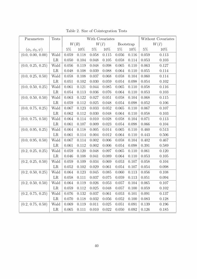
Table 2. Size of Cointegration Tests

Parameters Tests With Covariates Without Covariates

W (R) W (I) Bootstrap W (I)

(φ1, φ2, ψ) 5% 10% 5% 10% 5% 10% 5% 10%

(0.0, 0.00, 0.00) Wald 0.059 0.118 0.058 0.115 0.056 0.116 0.059 0.113

LR 0.050 0.104 0.048 0.105 0.058 0.114 0.053 0.103

(0.0, 0.25, 0.25) Wald 0.056 0.119 0.048 0.098 0.065 0.110 0.063 0.127

LR 0.048 0.108 0.039 0.088 0.064 0.110 0.055 0.114

(0.0, 0.25, 0.50) Wald 0.058 0.108 0.037 0.068 0.058 0.104 0.060 0.114

LR 0.051 0.102 0.030 0.059 0.054 0.098 0.054 0.102

(0.0, 0.50, 0.25) Wald 0.061 0.121 0.044 0.085 0.065 0.110 0.058 0.116

LR 0.054 0.113 0.036 0.076 0.064 0.110 0.053 0.103

(0.0, 0.50, 0.50) Wald 0.063 0.122 0.027 0.051 0.058 0.104 0.068 0.115

LR 0.059 0.112 0.025 0.048 0.054 0.098 0.052 0.106

(0.0, 0.75, 0.25) Wald 0.067 0.123 0.033 0.052 0.065 0.110 0.067 0.107

LR 0.062 0.112 0.030 0.048 0.064 0.110 0.058 0.103

(0.0, 0.75, 0.50) Wald 0.064 0.114 0.010 0.028 0.058 0.104 0.071 0.113

LR 0.061 0.107 0.009 0.023 0.054 0.098 0.066 0.104

(0.0, 0.95, 0.25) Wald 0.064 0.118 0.005 0.014 0.065 0.110 0.460 0.513

LR 0.061 0.114 0.004 0.012 0.064 0.110 0.443 0.506

(0.0, 0.95, 0.50) Wald 0.067 0.114 0.002 0.006 0.058 0.104 0.402 0.467

LR 0.061 0.112 0.002 0.006 0.054 0.098 0.391 0.589

(0.2, 0.25, 0.25) Wald 0.059 0.120 0.048 0.097 0.065 0.110 0.061 0.120

LR 0.046 0.108 0.041 0.089 0.064 0.110 0.053 0.105

(0.2, 0.25, 0.50) Wald 0.059 0.109 0.034 0.069 0.053 0.107 0.058 0.104

LR 0.052 0.102 0.029 0.061 0.054 0.107 0.054 0.098

(0.2, 0.50, 0.25) Wald 0.064 0.123 0.045 0.085 0.060 0.113 0.056 0.108

LR 0.058 0.111 0.037 0.075 0.059 0.113 0.051 0.094

(0.2, 0.50, 0.50) Wald 0.064 0.119 0.026 0.053 0.057 0.104 0.065 0.107

LR 0.059 0.112 0.025 0.048 0.057 0.100 0.059 0.102

(0.2, 0.75, 0.25) Wald 0.076 0.132 0.037 0.061 0.053 0.101 0.091 0.137

LR 0.070 0.118 0.032 0.056 0.052 0.100 0.083 0.128

(0.2, 0.75, 0.50) Wald 0.069 0.119 0.011 0.025 0.051 0.091 0.139 0.196

LR 0.065 0.111 0.010 0.022 0.050 0.092 0.126 0.185

40

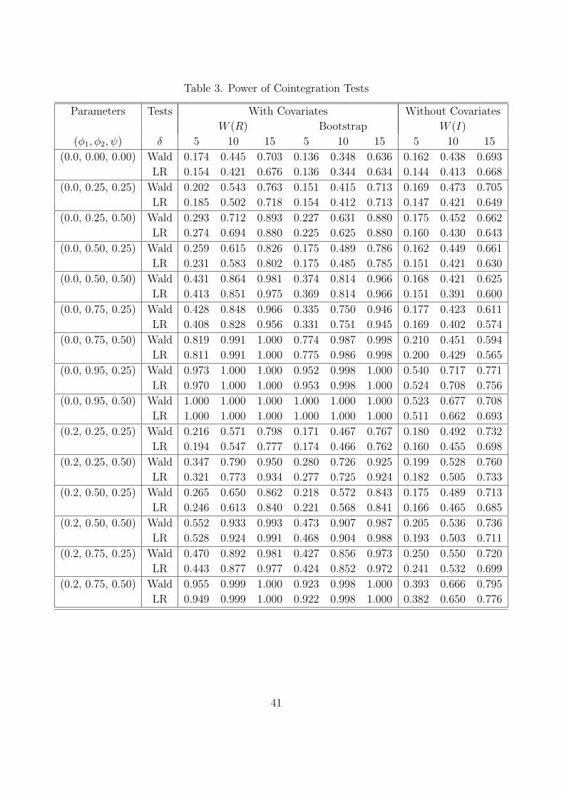
Table 3. Power of Cointegration Tests

Parameters Tests With Covariates Without Covariates

W (R) Bootstrap W (I)

(φ1, φ2, ψ) δ 5 10 15 5 10 15 5 10 15

(0.0, 0.00, 0.00) Wald 0.174 0.445 0.703 0.136 0.348 0.636 0.162 0.438 0.693

LR 0.154 0.421 0.676 0.136 0.344 0.634 0.144 0.413 0.668

(0.0, 0.25, 0.25) Wald 0.202 0.543 0.763 0.151 0.415 0.713 0.169 0.473 0.705

LR 0.185 0.502 0.718 0.154 0.412 0.713 0.147 0.421 0.649

(0.0, 0.25, 0.50) Wald 0.293 0.712 0.893 0.227 0.631 0.880 0.175 0.452 0.662

LR 0.274 0.694 0.880 0.225 0.625 0.880 0.160 0.430 0.643

(0.0, 0.50, 0.25) Wald 0.259 0.615 0.826 0.175 0.489 0.786 0.162 0.449 0.661

LR 0.231 0.583 0.802 0.175 0.485 0.785 0.151 0.421 0.630

(0.0, 0.50, 0.50) Wald 0.431 0.864 0.981 0.374 0.814 0.966 0.168 0.421 0.625

LR 0.413 0.851 0.975 0.369 0.814 0.966 0.151 0.391 0.600

(0.0, 0.75, 0.25) Wald 0.428 0.848 0.966 0.335 0.750 0.946 0.177 0.423 0.611

LR 0.408 0.828 0.956 0.331 0.751 0.945 0.169 0.402 0.574

(0.0, 0.75, 0.50) Wald 0.819 0.991 1.000 0.774 0.987 0.998 0.210 0.451 0.594

LR 0.811 0.991 1.000 0.775 0.986 0.998 0.200 0.429 0.565

(0.0, 0.95, 0.25) Wald 0.973 1.000 1.000 0.952 0.998 1.000 0.540 0.717 0.771

LR 0.970 1.000 1.000 0.953 0.998 1.000 0.524 0.708 0.756

(0.0, 0.95, 0.50) Wald 1.000 1.000 1.000 1.000 1.000 1.000 0.523 0.677 0.708

LR 1.000 1.000 1.000 1.000 1.000 1.000 0.511 0.662 0.693

(0.2, 0.25, 0.25) Wald 0.216 0.571 0.798 0.171 0.467 0.767 0.180 0.492 0.732

LR 0.194 0.547 0.777 0.174 0.466 0.762 0.160 0.455 0.698

(0.2, 0.25, 0.50) Wald 0.347 0.790 0.950 0.280 0.726 0.925 0.199 0.528 0.760

LR 0.321 0.773 0.934 0.277 0.725 0.924 0.182 0.505 0.733

(0.2, 0.50, 0.25) Wald 0.265 0.650 0.862 0.218 0.572 0.843 0.175 0.489 0.713

LR 0.246 0.613 0.840 0.221 0.568 0.841 0.166 0.465 0.685

(0.2, 0.50, 0.50) Wald 0.552 0.933 0.993 0.473 0.907 0.987 0.205 0.536 0.736

LR 0.528 0.924 0.991 0.468 0.904 0.988 0.193 0.503 0.711

(0.2, 0.75, 0.25) Wald 0.470 0.892 0.981 0.427 0.856 0.973 0.250 0.550 0.720

LR 0.443 0.877 0.977 0.424 0.852 0.972 0.241 0.532 0.699

(0.2, 0.75, 0.50) Wald 0.955 0.999 1.000 0.923 0.998 1.000 0.393 0.666 0.795

LR 0.949 0.999 1.000 0.922 0.998 1.000 0.382 0.650 0.776

41

Table 4. Money Demand Equation: 1960Q1-1999Q4

mt − pt yt rt

With Stationary Covariates

β 1 -1.3903 (0.2345) 0.0124 (0.0058)

α -0.0593 (0.0124) 0.0115 (0.0166) -0.0927 (1.5100)

R2 0.6989 0.4178 0.4645

Log-likelihood 590.77 553.56 -141.39

Q(1) 0.0563 [ 0.812 ] 0.0677 [ 0.795 ] 0.1247 [ 0.724 ]

Q(12) 9.5024 [ 0.660 ] 7.3507 [ 0.834 ] 15.791 [ 0.201 ]

ARCH LM(1) 0.6818 [ 0.410 ] 0.0003 [ 0.986 ] 0.0320 [ 0.858 ]

ARCH LM(12) 0.3911 [ 0.965 ] 0.6055 [ 0.834 ] 2.1492 [ 0.018 ]

Without Stationary Covariates

β 1 -1.1188 (0.3166) -0.0144 (0.0042)

α -0.0411 (0.0136) 0.0300 (0.0129) 2.7507 (1.4304)

R2 0.6552 0.3725 0.3625

Log-likelihood 580.36 547.79 -154.81

Q(1) 0.0087 [ 0.926 ] 0.0083 [ 0.927 ] 0.0006 [ 0.981 ]

Q(12) 12.042 [ 0.442 ] 7.1259 [ 0.849 ] 20.272 [ 0.062 ]

ARCH LM(1) 0.7832 [ 0.378 ] 0.0177 [ 0.894 ] 4.6330 [ 0.033 ]

ARCH LM(12) 0.8926 [ 0.556 ] 0.7394 [ 0.711 ] 10.225 [ 0.000 ]

The standard errors are in the parentheses, and the p-values are in the square brackets.

Table 5. Cointegration Tests: 1960Q1-1999Q4

WHn Wn LRn Wn LRn

Statistics 46.795 42.733 39.515 36.376 34.609

Asymptotic p-value 0.002 0.003 0.010 0.108 0.153

Bootstrap p-value 0.072 0.089 0.095 0.295 0.290

The canonical correlation R is estimated at (0.247, 0.973, 1.000).

42