OXFORD BULLETIN OF ECONOMICS AND STATISTICS, 48, 3 (1986)0305-9049 $3.00

DEVELOPMENTS IN THE STUDY OFCOINTEGRATED ECONOMIC VARIABLES

C. W. J. Granger*

I. INTRODUCTION

At the least sophisticated level of economic theory lies the belief thatcertain pairs of economic variables should not diverge from each otherby too great an extent, at least in the long-run. Thus, such variablesmay drift apart in the short-run or according to seasonal factors, butif they continue to be too far apart in the long-run, then economicforces, such as a market mechanism or government intervention, willbegin to bring them together again. Examples of such variables areinterest rates on assets of different maturities, prices of a commodity indifferent parts ofthe country, income and expenditure by local govern-ment and the value of sales and production costs of an industry. Otherpossible examples would be prices and wages, imports and exports,market prices of substitute commodities, money supply and prices andspot and future prices of a commodity. In some cases an economictheory involving equilibrium concepts might suggest close relations inthe long-run, possibly with the addition of yet further variables. How-ever, in each case the correctness of the beliefs about long-term related-ness is an empirical question. The idea underlying cointegration allowsspecification of models that capture part of such beliefs, at least for aparticular type of variable that is frequently found to occur in macro-economics. Since a concept such as the long-run is a dynamic one, thenatural area for these ideas is that of time-series theory and analysis.It is thus necessary to start by introducing some relevant time seriesmodels.

Consider a single series Xf, measured at equal intervals of time. Timeseries theory starts by considering the generating mechanism for theseries. This mechanism should be able to generate att of the statisticalproperties of the series, or at very least the conditional mean, varianceand temporal autocorrelations, that is the 'linear properties' of theseries, conditional on past data. Some series appear to be 'stationary',which essentially implies that the linear properties exist and are time-invariant. Here we are concerned with the weaker but more technical

* I would like to t^knowledge the excellent ho^itality that I enjoyed at Nuffield Collegeand the Institute of Eccaioinics and Statistics, Oxfoid whilst this papa was prepared.

213

2 1 4 BULLETIN

requirement that the series has a spectrum which is finite but non-zeroat all frequencies. Such a series will be called 7(0), denoting 'integratedof order zero'. Some series need to be differenced to achieve these pro-perties and these will be called integrated of order one, denoted .JC, ~ /(1).More generally, if a series needs differencing d times to become 7(0), itis called integrated of order cf, denoted x, ~ I{d). Let A* denote appli-cation of the difference operator b times, if x, ~7(d) then the Mhdifference series A'% is I{d — b). Sometimes a series needs to be inte-grated (summed) to become 7(0), for example the difference of an 7(0)series is 7( — 1) and its integral is again 7(0). Most of this paper will con-centrate on the practically important cases when d = Q or 1. Thesimplest example of an 7(0) series is a white noise e,, so that f>^ =corr(e,, e,_^)- 0 iov aWk^O. Another example is a stationary ARi\)series, x, generated by

JCf = oaf-i + e, (1.1)

where | a | < l and e, is white noise with zero mean. The simplestexample of an 7(1) series is a random walk, where x, is generated by

X, = x ,_ ,+ e, (1.2)

as would theoretically occur for a speculative price generated by aninformationally efficient market. Here, the first differenced series iswhite noise. The most general 7(1) series replaces e, in equation (1.2)by any 7(0) series not necessarily having zero mean. Many macro eco-nomic series appear to be 7(1), as suggested by the 'typical spectralshape' (see Granger (1966)), by analysis of Box-Jenkins (1970)modelling techniques or by direct testing, as in Nelson and Plosser(1982). Throughout the paper all error processes, such as those in(1.1), (1.2) are assumed to have finite first and second moments.

There are many substantial differences between 7(0) and 7(1)series. An 7(0) series has a mean and there is a tendency for the seriesto return to the mean, so that it tends to fluctuate around the mean,crossing that value frequently and with rare extensive excursions.Autocorrelations decline rapidly as lag increases and the process giveslow weights to events in the medium to distant past, and thus effectivelyhas a finite memory. An 7(1) process without drift will be relativelysmooth, will wander widely and will only rarely return to an earliervalue. In fact, for a random walk, for a fixed arbitrary value the expectedtime until the process again passes through this value is infinite. Thisdoes not mean that returns do not occur, but that the distribution ofthe time to return is very long-tailed. Autocorrelations {p^} are all nearone in magnitude even for laiige k\ an innovation to the process affectsall later values and so the process has indefinitely long memory. To seethis, note that the pure random walk 7( 1) solves to give

X, = e, + e,_i + e,_2 + . . . + e, (1.3)

DEVELOfMENTS IN THE STUDY OF COINTEGRATED ECONOMIC VARIABLES 2 1 5

assuming the process starts at time t = 0, with x^ = 0. Note that thevariance of x, is rof and becomes indefinitely large as t increases and

If X, is a random walk with 'drift' (1.2) becomes

where e, is zero-mean white noise. The solution is now

t-iX, = mr+ X e,_y (1.4)

/=o

so that Xf consists of a linear trend plus a drift-free /(1) process (randomwalk) being the process in (1.3). The only more general univariate pro-cess considered in this section is

where x,' is a drift-free random walk, such as generated by (1.3), andm(t) is some deterministic function of time, being the 'trend in mean'ofx,.

II. COINTEGRATION

Consider initially a pair of series x,, v,, each of which is 7( 1) and havingno drift or trend in mean. It is generally true that any linear combina-tion of these series is also 7(1). However, if there exists a constant A,such that

z, = x , - ^ > ' , (2.1)

is 7(0), then x,, y, will be said to be cointegrated, with A called thecointegrating parameter. If it exists, A will be unique in the situationnow being considered. As z, has such different temporal properties fromthose of either of its components it follows that the x, and y, must havea very special relationship. Both x, and >», have dominating low-frequencyor 'long wave' components, and yet z, does not. Thus, x, and y4>', musthave low-frequency components which virtually cancel out to produceZf. A good analogy is two series each of which contain a prominentseasonal component. Generally, any linear combination of these serieswill also contain a seasonal, but if the seasonals are identical in shapethere could exist a linear combination which has no seasonal.

The relationship

X, = Ay, (2.2)

might be considered a long-run or 'equilibrium' relationship, perhaps assuggested by some economic theory, and z, given by (2.1) thusmeasures the extent to which the system x,, y, is out of equilibrium.

2 1 6 BULLETIN

and can thus be called the 'equilibrium error'. The term 'equilibrium' isused in many ways by economists. Here the term is not used to implyanything about the behaviour of economic ^ents but rather describesthe tendency of an economic system to move towards a particularregion of the possible outcome space. If x, and j , are 1(1) but 'movetogether in the long-run', it is necessary that 2, be 7(0) as otherwise thetwo series will drift apart without bound. Thus, for a pair of 7(1) series,cointegration is a necessary condition for the ideas discussed in the firstsection of this paper to hold. In some circumstances, an even strongercondition may be required, such as putting complete bounds on z,,which wili guarantee that it is 7(0), but such cases are not consideredhere.

The extension to series having trends in their means is straightforward.Consider

where -v,',>v' ^re both 7(1) but without trends in mean, and let

y + x,'-Ayl.

For Z( to be 7(0), and Xj, j ' , not to drift too far apart, it is necessaryboth that Zf have no trend in mean, so that

t) (2.4)

for al! /, and that .v,', y^ be cointegrated with the same value of ^ asthe cointegrating parameter. It is seen that if the two trends in meanare different functions of time, such as an exponential and a cubic,then (2.4) cannot hold.

One thing that should be noted is that a model of the form

where Xj is 7(0) and 7, is 7(1), makes no sense as the independent anddependent variables have such vastly different temporal properties.Theoretically the only plausible value for ^ in this regression is j3 = 0.

If Xt, yt are both 7(1) without trends in mean and are cointegratedit has been proved in Granger (1983) and Granger and Engle (1985)that there always exists a generating mechanism having what is calledthe 'error-correcting' form:

where

Xf = - piz^_i + lagged (Ax,, Ayt) + d(5)eu

, = - P2^»-i + lagged (AXf, Ayt) + diB)

DEVELOPMENTS IN THE STUDY OF COINTCGRATED KIONOMIC VARIABLES 2 1 7

is a finite polynomial in the lag operator B (so thatand is the same in each equation, and Ci,, 62 are joint white noise,possibly contemporaneously correlated and with IPil + Ift! ^ 0 -Not only must cointegrated variables obey such a model but thereverse is also true; data generated by an error-correction model suchas (2.5) must be cointegrated. The reason for this is easily seen, as ifXt, yt are / (I) their changes will be /(O) and so every term in the equa-tions (2.5) is /(O) provided z, is also /(O) meaning that x,, j , are cointe-grated. If Zf is not 1(0), i.e., if x,,^^ are not cointegrated, then the z,term does not belong in these equations given that the dependentvariables are 1(0) and hence at least one of p, , p2 does not vanish.

These models were introduced into economics by Sargan (1964) andPhillips (1957) and have generated a lot of interest following the workof Davidson, Hendry, Srba and Yeo (1978), Hendry and von UngemSternberg (1980), Curry (1981), Dawson (1981) and Salmon (1982)amongst others. The models are seen to incorporate equilibriumrelationships, perhaps suggested by an economic theory of the long-run,with the type of dynamic model favoured by time-series econometri-cians. The equilibrium relationships are allowed to enter the model butare not forced to do so. The title 'error-correcting' for equations such as(2.5) is a little optimistic. The absolute value of z, is the distance thatthe system is away from equilibrium. Equation (2.5) indicates that theamount and direction of change in x, and y^ take into account the sizeand sign of the previous equilibrium error, Zf_i. The series z, does not,of course, certainly reduce in size from one time period to another butis a stationary series and thus is inclined to move towards its mean. Aconstant should be included in the equilibrium equation (2.2) and in(2.1) if needed, to make the mean of z, zero.

There are a number of theoretical implications of cointegratednessthat are easily derived from the results so far presented;

(i) If Xf, yf are cointegrated, so will be Xf and 6j ,_^ + Wf, for any kwhere w ~ / (0 ) , with a possible change in cointegrating para-meter. Formally, if Jc, is 1(1) then x, and jc,_fc will be cointe-grated for any k, but this is not an interesting property as it istrue for any 1(1) process and so does not suggest a specialrelationship, unlike cointegration of a pair of 1(1) series. Itfollows that if Xf, yt are cointegrated but are only observedwith measurement error, then the two observed series willalso be cointegrated if all measurement errors are 7(0).

(ii) If X, is 7(1) and fn^h(Jn) is the optimal forecast of Xn . , basedon the information set /„ available at time «, then Xt+h, ft,h(-ft)are cointegrated if /„ is a proper information set, that is if itincludes :<:„_;, / > 0. If /„ is not a proper information set, ^ .nand its optimum forecast are only cointegrated if Xf is cointe-grated with variables in /<.

2 1 8 BULUETIN

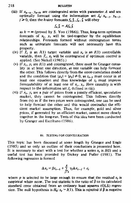
(iii) If Xn+ft, yn+h are cointegrated series with parameter A and areoptimally forecast using the information set Jn.Xn_j, yn-j,/• > 0, then the A-step forecasts^,^, J^, jU will obey

as /i -»• oo (proved by S. Yoo (1986)). Thus, Jong-term optimumforecasts of x,, y^ will be tied-together by the equilibriumrelationships. Forecasts formed without cointegration termssuch as univariate forecasts will not necessarily have thisproperty.

(iv) If Tf is an 7(1) target variable and x^ is an 7(1) controllablevariable, then T,, x, will be cointegrated if optimum control isapplied. (See Nickell (1985).)

(v) If Xf, >», are 7(1) and cointegrated, there must be Granger causa-lity in at least one direction, as one variable can help forecastthe other. This follows directly from the error-correlation mode!and the condition that Ipjl + IP2I "^0, as Zf._i must occur in atleast one equation and thus knowledge of z, must improveforecastability of at least one of Xf, y^. Here causahty is withrespect to the information set Jf defined in (iii).

(vi) If Xf, y'f are a pair of prices from a jointly efficient, speculativemarket, they cannot be cointegrated. This follows directlyfrom (v) as if the two prices were cointegrated, one can be usedto help forecast the other and this would contradict the effi-cient market assumption. Thus, for example, gold and silverprices, if generated by an efficient market, cannot move closelytogether in the long-run. Tests of this idea have been conductedby Granger and Escribano (1986).

in. TESTING FOR COINTEGRATION

This topic has been discussed at some length by Granger and Engle(1985) and so only an outline of their concliKions is presented here.It is necessary to start with a test for whether a series x, is 7(0) and auseful test has been provided by Dickey and Fuller (1981). Thefollowing regression is formed

Ax, = j3x,_i + Y, yA^t-i + et

where p is selected to be large enough to ensure that the residual e, isempirical white noise. The test statistic is the ratio ctf(3 to its calculatedstandard error obtained from an ordinary least squares (OLS) regres-sion. The null hypothesis isifo: Xf ~ 7(1). This is rejected if ^ is negative

DEVELOPMENTS IN THE STUDY OF COINTEGRATED ECONOMIC VARIABLES 2 1 9

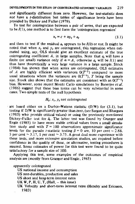
and significantly different from zero. However, the test-statistic doesnot have a f-distribution but tables of significance levels have beenprovided by Dickey and Fuller (1979).

To test for cointegration between a pair of series, that are expectedto be / ( I ) , one method is to first form the 'cointegration regression'

X, = c + a y , + 0, (3.1)

and then to test if the residual a, appears to be /(O) or not. It might benoted that when x^ and jf are cointegrated, this regression when esti-mated using, say, OLS should give an excellent estimate of the truecointegrating coefficient A, in large samples. Note that Of will have afinite (or small) variance only if a = ^ , otherwise a^ will be 7(1) andthus have theoretically a very large variance in a large sample. Stock(1984) has shown that when series are cointegrated, OLS estimatesof A are highly efficient with variances 0(7^^) compared to moreusual situations where the variances are 0(r~') , T being the samplesize. Stock also shows that the estimates are consistent with an 0(7""^)bias. However, some recent Monte Carlo simulations by Baneijee et al.(1986) suggest that these bias terms can be very substantial in somecases. Two simple tests of the null hypothesis

^0- Xf^yt iiot cointegrated

are based either on a Durbin-Watson statistic (D/W) for (3.1), buttesting if D/W is significantly greater than zero, (see Sargan and Bhargara(1983) who provide critical values) or using the previously mentionedDickey-Fuller test for df. The latter test was found by Granger andEngle (1985) to have more stable critical values from a small simula-tion study and with J = 100 observations approximate significancelevels for the pseudo /-statistic testing ^ = 0 are, 10 per cent ~ 2.88,5 per cent ~ 3.17, 1 per cent ~ 3.75. A great deal more experience withthese tests, and more extensive simulation studies, are required beforeconfidence in the quality of these, or alternative, testing procedures isassured. Some estimates of power for this test were found to be quitesatisfactory for a sample size of 100.

Applying this test, some examples of the outcomes of empiricalanalysis are (mostly from Granger and Engle, 1985)

apparently cointegratedUS national income and consumptionUS non-durables, production and salesUS short and long-term interest ratesUK W, P, H, U, T, (Hall, - this issue)UK Velocity and short-term interest rates (Hendry and Erics«)n,

1983)

2 2 0 BULLETIN

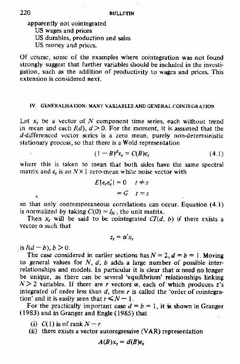
apparently not cointegratedUS wages and pricesUS durables, production and salesUS money and prices.

Of course, some of the examples where cointegration was not foundstrongly suggest that further variables should be included in the investi-gation, such as the addition of productivity to wages and prices. Thisextension is considered next.

IV. GENERALISATION: MANY VARIABLES AND GENERAL COINTEGRATION

Let X, be a vector of A component time series, each without trendin mean and each I(d), d> 0. For the moment, it is assumed that thefi?-differenced vector series is a zero mean, purely non-deterministicstationary process, so that there is a Wold representation

(l-.S)''A:, = a^ ) e , (4.1)

wliere this is taken to mean that both sides have the same spectralmatrix and e, is an A X 1 zero-mean white noise vector with

= G t=s

so that only contemporaneous correlations can occur. Equation (4.1)is normalized by taking C(0) = Ij^, the unit matrix.

Then x^ will be said to be cointegrated CI(d, b) if there exists avector a such that

z, = a%

isI(d-b),b>0.The case considered in earlier sections hasA^ = 2,d = b = 1. Moving

to general values for N, d, b adds a large number of possible inter-relationships and models. In particular it is clear that a need no longerbe unique, as there can be several 'equilibrium' relationships linkingA > 2 variables. If there are r vectors a, each of which produces z'sintegrated of order less than d, then r is called the 'order of cointegra-tion' and it is easily seen that r < A — 1.

For the practically important case d = 6 = 1, it K shown in Granger(1983) and in Granger and Engle (1985) that

(i)(ii) there exists a vector autoregressive (VAR) representation

DEVELOPMENTS IN THE STUDY OF COINTEGRATED ECONOMIC VARIABLES 2 2 1

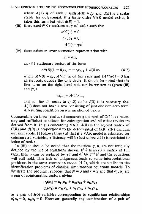
where ^(1) is of rank r with i4(0) =4r and d{B) is a scalarstable lag polynomial. If a finite order VAR model exists, ittakes this form but with d{B) = 1.

(iii) there exist NX r matrices a, y of rank r such that

(iv) there exists an error-correction representation with

2, = a'xt

an r X 1 stationary vector, of the form

A*{B){1 -B)x, = - Tz,_i + d{B)et (4.2)

where A*(O)=I]y, A*0) is of full rank and \A*(w)\ = 0 hasall its roots outside the unit circle. It should be noted that thefirst term on the right hand side can be written as (given (iii)and (v))

and so, for all terms in (4.2) to be 7(0) it is necessary that.4(1) does not have a row consisting of just one non-zero term.A resulting condition on o: is mentioned below.

Commenting on these results, (i) concerning the rank of C( 1) is a neces-sary and sufficient condition for cointegration and all other results arederived from it. In (ii) concerning VAR, A{B) is the adjoint matrix ofC(B) and d(B) is proportional to the determinant of C(B) after dividingout unit roots. It follows from (ii) that if a VAR model is estimated forcointegrated variables, efficiency will be lost unless .4(1) is restricted tobeing of rank r.

In (iii) it should be noted that the matrices y, a, are not uniquelydefined by the set of equations shown. If 6 is an rX r matrix of fullrank, then y can be replaced by y6 and a' by d~^a' and the equationswill still hold. This lack of uniqueness leads to some interpretationalproblems in the error-correction model (4.2), which are similar to theidentification problems of classical simultaneous equations models. Toillustrate the problem, suppose that A' = 3 and r — 2 and that ttj, Oj area pair of cointegrating vectors, giving

as a pair of 7(0) variables corresponding to equilibrium relationshipsi = 0, ajjc, = 0. However, generally any combination of a pair of

222 BULLETIN

7(0) variables will also be 7(0) and so

will also be 7(0) I it is assumed that for no X will z,(X) consist of justone component of Jt,: this is a constraint on the matrix a preventingz,(X) = Xf, for example, which would make z, ~7(1)]. Thus, the equili-brium relations are not uniquely identified, and the error-correctionmodels cannot be strictly interpreted as 'correcting' for deviations froma particular pair of equilibrium relationships. The only invariantrelationship is the line in the (Xf ,X2,Xj) space defined by

This same line is given by

for any Xj # X2 and will be called the 'equilibrium sub-space'. The error-correction mode! might thus be interpreted as Ax^ being influenced bythe distance the system is from the equilibrium sub-space. For generalA , r, the equilibrium sub-space will be a hyper-plane of dimension N—r.

It is unclear if the identification question can be solved in wayssimilar to those used with simultaneous equations, that is by addingsufficient zeros to y4( 1) or by appeals to 'exogeneity'.

For the TV = 3, /• = 2 case, X's can be chosen to give

Z, = OC^Xtf +

and

and these seem to provide a natural way for testing for cointegration.For more general A and r, the number of possible combinationsbecomes extensive and testing will be more difficult, particularly whenr is an unknown, as will be usual in practice.

Turning briefly to the most general case, with any A , d, b and r, theerror-correction model becomes

A*(B)(l -B)\ = -7KI - ( I -Bf](\

(4.3)

where d(B) is a scalar polynomial in B.It should be noted that {1 ~ ( 1 ~"-B)*], if expanded in powers of

B, has no term in 5° and so only lagged z, occur on the right handside. Again, every term in (4.3) is 7(0) when cointegration is present.It is possible to define fractional differencing, as in Granger and Joyeux(1980), and equation (4.3) still holds in this case, a t t h o i ^ its practicalimportance has yet to be established.

DEVELOPMENTS IN THE STUDY OF COINTEGRATED ECONOMIC VARIABLES 2 2 3

In the general case (with integer N,b,d,r) Yoo (1986) has consideredalternative ways of defining the z/s possibly using lagged Xf components,for a given C(B) matrix but with some added assumptions about itsform. Johanssen (1985) has also found some mathematically exact andattractive results for the general case, which do not rely on the assump-tion that all components of x, are integrated of the same order. Hepoints out, for example, that if X(, is / (I) and X2t is 1(0), then x,, andX2t — ^/=o Xzj^j could be cointegrated, thus expanding the classof variables that might be tested.

The work of Yoo and Johanssen suggests a more general definition ofcointegration. Let Oi{B) be an iV X 1 vector of functions of the lag opera-tor B, such that each component, such as a,(fi) has the property thatOLj( 1) ¥= 0. Then if x, is a vector of I{d) series such that

is lid — b), Xf may be called cointegrated. If a cointegrating vector aoccurs, as defined in earlier sections there will be many a(B) that alsocointegrate, and so uniqueness is lost but extra flexibility is gained.Consideration of these possibilities does allow for a generalisa-tion that is potentially very important in economics. Suppose thatN = 2,so that X, has just two components, and let a be a cointegratingvector, with a' = (1,.4). In this case a will be unique, if it does notdepend on B, so that r = I. [Generally, one would expect r<N] .However, there may exist another cointegrating vector of quite adifferent form.

« ' = (1,—i4') and A = 1 —B. An example of this possibility is where^ = iXt,)'t),Xt,yt are cointegrated with vector a, giving equilibriumerror:

and Xf, SZf = S/=o z,_; are cointegrated, so that Xf—A'SZf is 7(0). Thiswould correspond to a cointegrating vector of the form

a(£) = (l -SA',SAA')

where 5 = I/A and A = 1 - . 6 .For example, x,, y^ could be sales and production of some industry,

Zf = change in inventory, SZf inventory and x,, j , could be cointegratedas well as x,, SZf. Another example might be x, = income, j ' , = expendi-ture, Zf = savings, SZf = wealth. Such series might be called 'multi-coin tegrated'.

2 2 4 BULLETIN

Throughout this section, if the series involved have deterministictrends in mean, these need to be estimated and removed before theconcepts discussed can be applied. One method of removing trends ofgeneral shape is discussed in Granger (1985).

V. FURTHER GENERALIZATIONS

The processes considered so far have been linear and with time-invariantparameters. Clearly general models, and possibly more realistic ones, areachieved by removing these restrictions.

As institutions, technology and society changes, so may any equili-brium relationships. In the bivariate case, the cointegrating parametermay be slowly changing with time, for instance. To proceed withanalysis of this idea, it is necessary to define time-varying parameter(TVP) 7(0) and 7(1) processes. Using concepts introduced by Priestley(1981), it is possible to define a time-varying spectrum/,(w) for a pro-cess such as one generated by an ARMA model with TVP. For example,consider

Xt = mxt-i + et

where P(t) is a deterministic function of time, obeying the restrictionthat \^it)\ < 1 all t. If/f(w) is bounded above and also is positive forall ?, H', the process may be called TVP 7(0). If the change of jc, is TVP7(0), then JC, can be called TVP 7( 1).

For a vector process Xf that is TVP 7(d) and has no deterministiccomponents Cramer (1961) has shown that there exists a generalisedWold representation

{\-B)\ = CtiB)et (5.1)

where

= 0

= 0

and if

Ct(B) = 2

it will be assumed that

i

so that the variance of (1 — B'fxt is finite.

DEVELOPMENTS IN THE STUDY OF COINTEGRATED ECONOMIC VARIABLES 2 2 5

Assume now that Q( l ) has rank A — 1 for all t, so that the cointegra-tion rank is 1, then there will exist iVX 1 vectors a(t), y(t) such that

The TVP equilibrium error process will then be

' (5.2)

The corresponding error-correction models will be as (4.2) but withA*iB), y, d{B) all functions of time. A testing procedure would involveestimating the equilibrium regression (5.2) using some TVP techniques,such as a Kalman filter procedure, probably assuming that the com-ponents of ot{r) are stochastic but slowly changing.

It might be thought that allowing a{t) to change with time canalways produce an 7(0) z,. For example, suppose that Af = 2 and consider

Taking A{t) = Xfly^ clearly gives z, = 0, which is an uninteresting 7(0)situation. However, it is also clear that taking, A (t) - Xj/j, + 6 willproduce a z, that is 7(1) in general. Interpretation of any TVP cointegra-tion test will have to consider this possible difficulty.

Turning to the possibility of non-linear cointegration, it might benoted that in the basic error-correlation model (2.5) or (4.2) Zf_i termsappear linearly so that changes in dependent variables are related toZf_], whatever its size. In the actual economy, a more realistic behaviouris to ignore small equilibrium errors but to react substantially to largeones, suggesting a non-linear relationship. An error-correction mode!that captures this idea is, in the bivariate case.

t=f\%-i) + lagged(AXf, Aj^) + ej,

'f = /2(Zr-i) + lagged (AXf, Aj,) ^ e^t

where

z, = x,-^:i'f.

It is generally true that if z, is 7(0) with constant variance, then/(Zr)will also be 7(0). Similarly, if z, is 7(1) then generally /(z,) is also 7(1),provided /(z) has a linear component for large z, i.e. fl2{z) -*• S^o UjZ'with a^i^O. A rigorous treatment of these results is provided by Escri-bano (1986). As generally z, and f{Zf) will be integrated of the sameorder, if a test suggests that a pair of series are cointegrated, then a non-linear error-correction model of form (5.3) is a possibility. Of course,most of the other results of previous sections do not hold as they arebased on the linear Wold representation. Equation (5.3) can be esti-mated by one of the many currently available non-linear, non-para-

2 2 6 BULLETIN

metric estimation techniques such as that employed in Engle, Granger,Rice and Weiss (1986).

Error correction models essentially consider process whose com-ponents drift widely but the joint process has a generalised preferencetowards a certain part of the process space. In the cases so far consideredthis preferred sub-space is a hyper-plane but more general preferred sub-spaces could be considered although with considerably increased mathe-matical difficulty.

VI. CONCLUSION

This paper has attempted to expand the discussion about differencingmacro-economic series when model building by emphasizing the use ofa further factor, the 'equilibrium error', that arises from the concept ofcointegration. This factor allows the introduction of the impact of long-run or 'equilibrium' economic theories into the models used by thetime-series analysts to explain the short-run dynamics of economicdata. The resulting error-correction models should produce bettershort-run forecasts and will certainly produce long-run forecasts thathold together in economically meaningful ways.

If long-run economic theories are to have useful impact on econo-metric models they must be helpful in model specification and yetnot distract from the short-run aspects of the model. Historically, manyeconometric models were based on equilibrium relationships suggestedby a theory,such as

Xf = Ayf + ef (6.1)

without any consideration of the levels of integratedness of the observedvariables Xf, yf or of the residual series e,. If x, is 7(0) but>', is 7(1), forexample, the value of ^ in the resulting regression is forced to be nearzero. If ef is 7(1), standard estimation techniques are not appropriate.A test for cointegration can thus be thought of as a pre-test to avoid'spurious regression' situations. Even if Xf and >>, are cointegrated anequation such as (6.1) can only provide a start for the modelling pro-cess, as e, may be explainable by lagged changes inx^and^',, eventuallyresulting in an error-correction model of the form (2.5). However,there must be two such equations, which again makes the equation(2.5) a natural form. Ignoring the process of properly modelling thee, can lead to forecasts from (6.1) that can be beaten by simple time-series models, at least in the short-term.

Whilst the paper has not attempted to link error-correction modelswith optimizing economic theory, through control variables forexample, there is doubtless much useful work to be done in this area.

Testing for cointegration in general situations is stai in an early stageof development. Whether or not cointegration occurs is an empirical

DEVELOPMENTS IN THE STUDY OF COINIEGRATED ECONOMIC VARIABLES 2 2 7

question but the beliefs of economists do appear to support its existenceand the u^fulness of the concept appears to be rapidly gainingacceptance.

University of California. San Diego

Date of Receipt of Final Manusayjt: April 19S6

REFERENCES

Box, G. E.P. and Jenkins, C M . (1970). Time Series Analysis Forecasting and Con-trol, San Francisco, Holden Day.

Cramer, H. (1961). 'On Some Classes of Non-Stationary Processes', Proceedings4th Berkeley Symposium on Math, Stats and Probability, pp. 157-78, Univer-sity of California Press.

Currie, D. (1981). 'Some Long-Run Features of Dynamic Time-Series Models',The Economic Journal,Vol. 363, pp. 704-15.

Davidson, J. E. H., Hendry, D. F., Srba, F. and Yeo, S. (1978). 'Econometric Model-ling of the A^regate Time^Series Relationship Between Consumer's Expendi-ture and Income in the United Kingdom', The Economic Journal, Vol. 88,pp. 661-92.

Dawson, A. (1981). 'Saigan's Wage Equation: A Theoretical and Empirical Recon-struction', j4pp/ierf£'co«oi?iics. Vol. 13, pp. 351-63.

Dickey, D. A. and Fuller, W. A. (1979). 'Distributions of the Estimators foT Auto-regressive Time Series with a Unit Root', Journal of the American StatisticalAssociation, Vol. 74, pp. 427-31.

Dickey, D. A. and Fuller, W. A. (1981). 'The Likelihood Ratio Statistics for Auto-regreffiive Time Series with a Unit Root, Econometrica, Vol. 49, pp. 1057-72.

Engle, R. F., Giangei, C. W. J., Rice, J. and Weiss, A. (1986). 'Non-ParametricEstimation of the Relationship Between Weather and Electricity Demand',Journal of the American Statistical Association,{io'[i}[icoT!m%).

Escribano, A. (1986). PhX>. thesis, Economics Department, University of Cali-fornia, San Diego.

Granger, C. W. J. (1966). 'The Typical Spectral Shape of an Economic Variable',Econometrica, Vol. 34, pp. 150-61.

Granger, C. W. J. (1983). 'Co-Integiated Variables and Error-Correcting Models',UCSD Discussion Paper, pp. 83-13a.

Granger, C. W. J. and Engle, R. F. (1985). 'Dynamic Specification with EquilibriumConstraints: Cointegration and Error-Correction', (forthcoming, Econometrica).

Grai^er, C. W. J. and Escribano, A. (1986). 'Limitation on the Lxing-Run Relation-ship Between Prices from an Efficient Market', UCSD Discussion Paper.

Granger, C. W. J. and Joyeux, R. (1980). 'An Introduction to Long-Memory TimeSeries and Fractional Differencing', Journal of Time Series Analysis, Vol. 1,pp. 15-29.

Hendry, D. F. and Ericsson, N. R. (1983). 'Assertion without Empirical Basis: AnEconometric Appraisal of ''Monetary Trends in . . . the United Kingdom" byMilton Friedman and Anna Schwartz', Bank of England Academic Panel Papa-No. 22

228 BULLETIN

Hendry, D. F. and von Ungem-Stemberg,T. (1981). 'Liquidity and Inflation Effectson Consumer's Expenditure', in Deaton, A. S. (ed.), Essex's in the Theory andMeasurement of Consumer's Behaviour, Cambridge Univeisity Press.

Johanssen, S. (1985). 'The Mathematical Structure of Error-Correction Modeis',Discussion Paper, Maths Department, University of Copenh^en.

Nelson, C. R. and Plosser, C. I. (1982). 'Trends and Random WaJks in Macro-economic Time ^XK%\ Joumal of Monetary Economics,Vol. 10, pp. 139-62.

Nickell, S. (1985). 'Error-Correction, Partial Adjustment and all that: an Exposi-tory Note', BULLETIN, Vol. 47, pp. 119-29.

Phillips, A. W. (1957). 'Stabilization Policy and the Time Forms of Lagged Res-ponses', fcortomzc Joumal, VoL 67, pp. 265-77.

Priestley, M. B. (198 i). Spectral Analysis of Time Series, Academic Press, NewYork.

Salmon, M. (1982). 'Error Correction Mechanians', The Economic Journal, Vol. 92,pp. 615-29.

Sargan, J. D. (1964). 'Wages and Prices in the United Kingdom: A Study in Econo-mic Methodology', in Hart, P., Mills, G. and Whittaker, J. N. (eds.). EconometricAnalysis for National Economic Planning, Butterworths, London.

Sargan, J. D. and Bhargava, A. (1983). 'Testing Residuals from Least SquaresRegression for being generated by the Gaussian Random Walk', Econometrica,Vol. 51, pp. 153-74.

Stock, J. H. (1984). 'Asymptotic Properties of a Least Squares Estimator of Co-Integrating Vectors', manuscript Harvard University.

Yoo, S. (1986). PhD. thesis. Economics Etepartment, University of California,San Diego.